Random Features for Large Scale Kernel

MachinesAndrea Vedaldi

From: A. Rahimi and B. Recht. Random features for large-scale kernel machines. In Proc. NIPS, 2007.

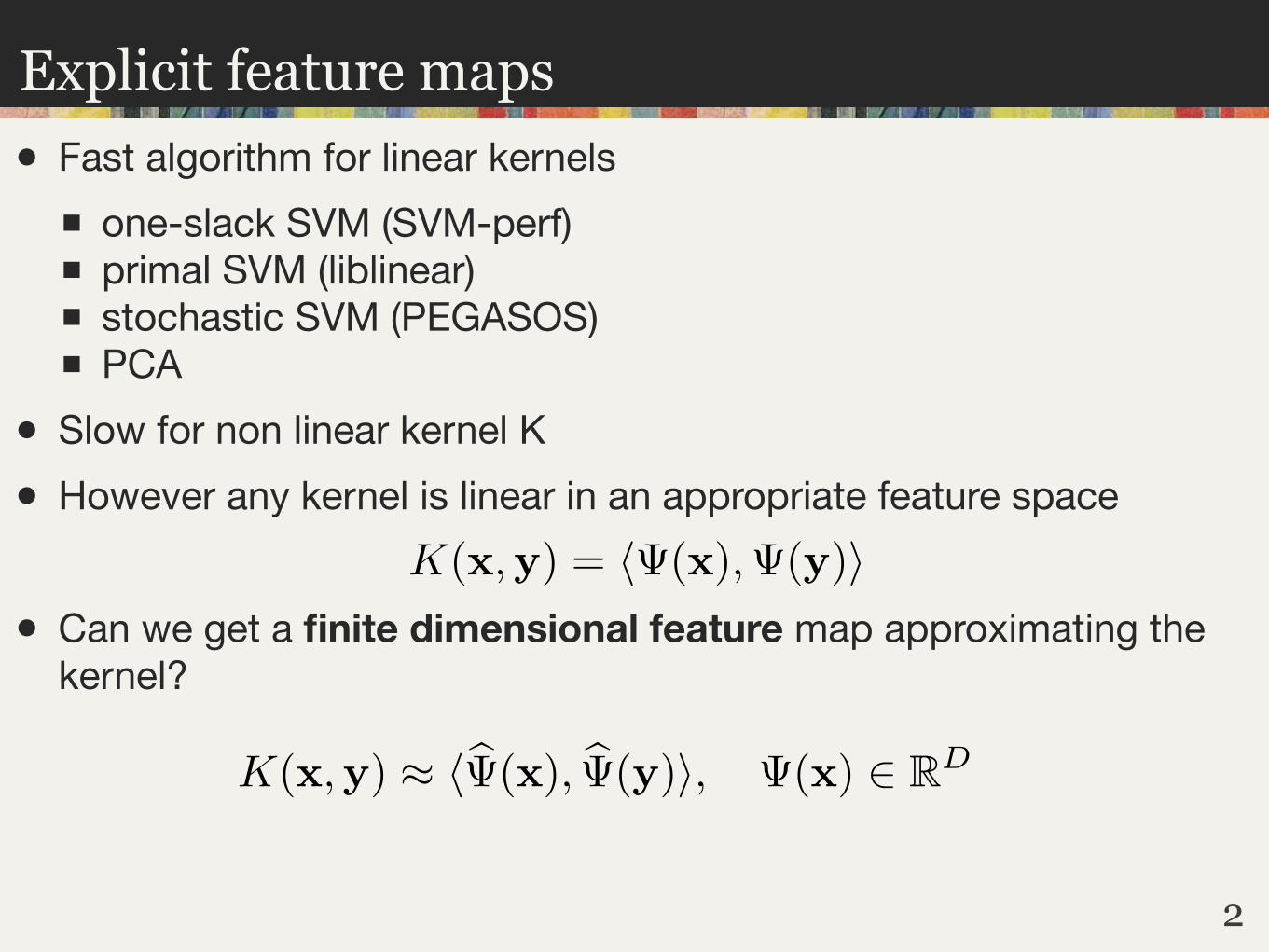
Explicit feature maps• Fast algorithm for linear kernels

one-slack SVM (SVM-perf) primal SVM (liblinear) stochastic SVM (PEGASOS) PCA

• Slow for non linear kernel K

• However any kernel is linear in an appropriate feature space

• Can we get a finite dimensional feature map approximating the kernel?

2

Random Fourier features 1/2• Translation invariant kernel: K(x,y) = K(y - x)

• BochnerIf K is PD and translation invariant, then

for some real, symmetric, non neg. measure κ(λ) dλ.

• Bochner as expected valueIf K(0) = 1 (normalized), then

3

Random Fourier features 2/2• Random Fourier features

Obtain approximate feature map from random sampling

• Gaussian random Fourier features

MATLAB pseudocodefunction psix = gaussianRandomFeatures(x, D)d = size(x, 1) ;omega = randn(D, d) ;psix = exp(-i*omega*x) ; 4

Random Fourier features: Errors

• Uniform error bound in a ball

(with any fixed probability) requires

random projections.

5

RD

R2ω

xKernel Name k(∆) p(ω)

Gaussian e−∆22

2 (2π)−D2 e−

ω222

Laplacian e−∆1

d1

π(1+ω2d)

Cauchy

d2

1+∆2d

e−∆1

Figure 1: Random Fourier Features. Each component of the feature map z(x) projects x onto a randomdirection ω drawn from the Fourier transform p(ω) of k(∆), and wraps this line onto the unit circle in R2.After transforming two points x and y in this way, their inner product is an unbiased estimator of k(x,y). Thetable lists some popular shift-invariant kernels and their Fourier transforms. To deal with non-isotropic kernels,the data may be whitened before applying one of these kernels.

If the kernel k(δ) is properly scaled, Bochner’s theorem guarantees that its Fourier transform p(ω)is a proper probability distribution. Defining ζω(x) = ejωx, we have

k(x− y) =

Rd

p(ω)ejω(x−y) dω = Eω[ζω(x)ζω(y)∗], (2)

so ζω(x)ζω(y)∗ is an unbiased estimate of k(x,y) when ω is drawn from p.

To obtain a real-valued random feature for k, note that both the probability distribution p(ω) andthe kernel k(∆) are real, so the integrand ejω(x−y) may be replaced with cos ω(x − y). Definingzω(x) = [ cos(x) sin(x) ] gives a real-valued mapping that satisfies the condition E[zω(x)zω(y)] =k(x,y), since zω(x)zω(y) = cos ω(x − y). Other mappings such as zω(x) =

√2 cos(ωx +

b), where ω is drawn from p(ω) and b is drawn uniformly from [0, 2π], also satisfy the conditionE[zω(x)zω(y)] = k(x,y).

We can lower the variance of zω(x)zω(y) by concatenating D randomly chosen zω into a columnvector z and normalizing each component by

√D. The inner product of points featureized by the

2D-dimensional random feature z, z(x)z(y) = 1D

Dj=1 zωj (x)zωj (y) is a sample average of

zωj (x)zωj (y) and is therefore a lower variance approximation to the expectation (2).

Since zω(x)zω(y) is bounded between -1 and 1, for a fixed pair of points x and y, Hoeffd-ing’s inequality guarantees exponentially fast convergence in D between z(x)z(y) and k(x,y):Pr [|z(x)z(y)− k(x,y)| ≥ ] ≤ 2 exp(−D2/2). Building on this observation, a much strongerassertion can be proven for every pair of points in the input space simultaneously:

Claim 1 (Uniform convergence of Fourier features). Let M be a compact subset of Rd with diam-eter diam(M). Then, for the mapping z defined in Algorithm 1, we have

Pr

supx,y∈M

|z(x)z(y)− k(x,y)| ≥

≤ 28

σp diam(M)

2

exp− D2

4(d + 2)

,

where σ2p ≡ Ep[ωω] is the second moment of the Fourier transform of k. Fur-

ther, supx,y∈M |z(x)z(y) − k(y,x)| ≤ with any constant probability when D =

Ω

d2 log σp diam(M)

.

The proof of this assertion first guarantees that z(x)z(y) is close to k(x − y) for the centers of an-net over M ×M. This result is then extended to the entire space using the fact that the featuremap is smooth with high probability. See the Appendix for details.

By a standard Fourier identity, the scalar σ2p is equal to the trace of the Hessian of k at 0. It

quantifies the curvature of the kernel at the origin. For the spherical Gaussian kernel, k(x,y) =exp

−γx− y2

, we have σ2

p = 2dγ.

3

Gaussian kernelvariance

Accuracyrequired

Datadimensionality

Validityrange

Random Binning features 1/2

• indicator vector for the bin occupied by x under shift u

6

B0 B1 B2 B3B-1B-2

δu

Randomly shifted bins of side δ

x

δ

xHat kernel

Random binning features 2/2• Decompose other kernels as averages over hat kernels

it’s a simple deconvolution problem solved by

• Assuming that

interpret p(δ) as a probability density expand kernel as

where- uj ~ uniformly at random in [0, δ]- δj ~ p(δ)

7

Random binning features 3/3• Separable kernel

represent as the probability of being binned together simultaneously in the d dimensions

• Remarks

The feature map has very high dimension, but it is very sparse Must be stored in a hash structure Convergence rates similar to the random Fourier features

8

Experiments

9

Dataset Fourier+LS Binning+LS CVM Exact SVMCPU 3.6% 5.3% 5.5% 11%

regression 20 secs 3 mins 51 secs 31 secs

6500 instances 21 dims D = 300 P = 350 ASVM

Census 5% 7.5% 8.8% 9%

regression 36 secs 19 mins 7.5 mins 13 mins

18,000 instances 119 dims D = 500 P = 30 SVMTorch

Adult 14.9% 15.3% 14.8% 15.1%

classification 9 secs 1.5 mins 73 mins 7 mins

32,000 instances 123 dims D = 500 P = 30 SVMlight

Forest Cover 11.6% 2.2% 2.3% 2.2%

classification 71 mins 25 mins 7.5 hrs 44 hrs

522,000 instances 54 dims D = 5000 P = 50 libSVM

KDDCUP99 (see footnote) 7.3% 7.3% 6.2% (18%) 8.3%

classification 1.5 min 35 mins 1.4 secs (20 secs) < 1 s

4,900,000 instances 127 dims D = 50 P = 10 SVM+sampling

Table 1: Comparison of testing error and training time between ridge regression with random features, Core

Vector Machine, and various state-of-the-art exact methods reported in the literature. For classification tasks,

the percent of testing points incorrectly predicted is reported, and for regression tasks, the RMS error normal-

ized by the norm of the ground truth.

100 102 104 106

0.1

0.2

0.3

0.4

0.5

Training set size

Test

ing

erro

r

10 20 30 40 502

3

4

5

6

P

% e

rror

10 20 30 40 50

400

800

1200

P

train

ing+

test

ing

time

(sec

)

Figure 3: Accuracy on test data continues to improve as the training set grows. On the Forest dataset, using

random binning, doubling the dataset size reduces testing error by up to 40% (left). Error decays quickly as Pgrows (middle). Training time grows slowly as P grows (right).

minw Zw − y22 + λw2

2, where y denotes the vector of desired outputs and Z denotes the

matrix of random features. To evaluate the resulting machine on a datapoint x, we can simply

compute wz(x). Despite its simplicity, ridge regression with random features is faster than, and

provides competitive accuracy with, alternative methods. It also produces very compact functions

because only w and a set of O(D) random vectors or a hash-table of partitions need to be retained.

Random Fourier features perform better on the tasks that largely rely on interpolation. On the other

hand, random binning features perform better on memorization tasks (those for which the standard

SVM requires many support vectors), because they explicitly preserve locality in the input space.

This difference is most dramatic in the Forest dataset.

Figure 3(left) illustrates the benefit of training classifiers on larger datasets, where accuracy con-

tinues to improve as more data are used in training. Figure 3(middle) and (right) show that good

performance can be obtained even from a modest number of features.

6 Conclusion

We have presented randomized features whose inner products uniformly approximate many popular

kernels. We showed empirically that providing these features as input to a standard linear learning

algorithm produces results that are competitive with state-of-the-art large-scale kernel machines in

accuracy, training time, and evaluation time.

It is worth noting that hybrids of Fourier features and Binning features can be constructed by con-

catenating these features. While we have focused on regression and classification, our features can

be applied to accelerate other kernel methods, including semi-supervised and unsupervised learn-

ing algorithms. In all of these cases, a significant computational speed-up can be achieved by first

computing random features and then applying the associated linear technique.

6

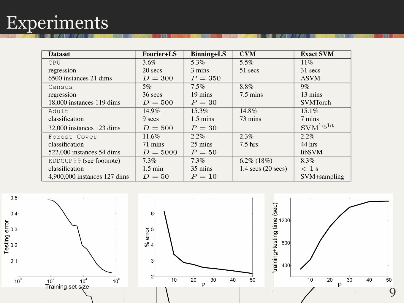
Dataset Fourier+LS Binning+LS CVM Exact SVMCPU 3.6% 5.3% 5.5% 11%

regression 20 secs 3 mins 51 secs 31 secs

6500 instances 21 dims D = 300 P = 350 ASVM

Census 5% 7.5% 8.8% 9%

regression 36 secs 19 mins 7.5 mins 13 mins

18,000 instances 119 dims D = 500 P = 30 SVMTorch

Adult 14.9% 15.3% 14.8% 15.1%

classification 9 secs 1.5 mins 73 mins 7 mins

32,000 instances 123 dims D = 500 P = 30 SVMlight

Forest Cover 11.6% 2.2% 2.3% 2.2%

classification 71 mins 25 mins 7.5 hrs 44 hrs

522,000 instances 54 dims D = 5000 P = 50 libSVM

KDDCUP99 (see footnote) 7.3% 7.3% 6.2% (18%) 8.3%

classification 1.5 min 35 mins 1.4 secs (20 secs) < 1 s

4,900,000 instances 127 dims D = 50 P = 10 SVM+sampling

Table 1: Comparison of testing error and training time between ridge regression with random features, Core

Vector Machine, and various state-of-the-art exact methods reported in the literature. For classification tasks,

the percent of testing points incorrectly predicted is reported, and for regression tasks, the RMS error normal-

ized by the norm of the ground truth.

100 102 104 106

0.1

0.2

0.3

0.4

0.5

Training set size

Test

ing

erro

r

10 20 30 40 502

3

4

5

6

P

% e

rror

10 20 30 40 50

400

800

1200

P

train

ing+

test

ing

time

(sec

)

Figure 3: Accuracy on test data continues to improve as the training set grows. On the Forest dataset, using

random binning, doubling the dataset size reduces testing error by up to 40% (left). Error decays quickly as Pgrows (middle). Training time grows slowly as P grows (right).

minw Zw − y22 + λw2

2, where y denotes the vector of desired outputs and Z denotes the

matrix of random features. To evaluate the resulting machine on a datapoint x, we can simply

compute wz(x). Despite its simplicity, ridge regression with random features is faster than, and

provides competitive accuracy with, alternative methods. It also produces very compact functions

because only w and a set of O(D) random vectors or a hash-table of partitions need to be retained.

Random Fourier features perform better on the tasks that largely rely on interpolation. On the other

hand, random binning features perform better on memorization tasks (those for which the standard

SVM requires many support vectors), because they explicitly preserve locality in the input space.

This difference is most dramatic in the Forest dataset.

Figure 3(left) illustrates the benefit of training classifiers on larger datasets, where accuracy con-

tinues to improve as more data are used in training. Figure 3(middle) and (right) show that good

performance can be obtained even from a modest number of features.

6 Conclusion

We have presented randomized features whose inner products uniformly approximate many popular

kernels. We showed empirically that providing these features as input to a standard linear learning

algorithm produces results that are competitive with state-of-the-art large-scale kernel machines in

accuracy, training time, and evaluation time.

It is worth noting that hybrids of Fourier features and Binning features can be constructed by con-

catenating these features. While we have focused on regression and classification, our features can

be applied to accelerate other kernel methods, including semi-supervised and unsupervised learn-

ing algorithms. In all of these cases, a significant computational speed-up can be achieved by first

computing random features and then applying the associated linear technique.

6