randomized experiments from non-random selection in u.s ...davidlee/wp/rdrand.pdfjournal of...
TRANSCRIPT

ARTICLE IN PRESS
0304-4076/$ - se
doi:10.1016/j.je
$An earlier
discontinuity an�Tel.: +1 60
E-mail addr
Journal of Econometrics 142 (2008) 675–697
www.elsevier.com/locate/jeconom
Randomized experiments from non-random selection inU.S. House elections$
David S. Lee�
Department of Economics and Woodrow Wilson School, Princeton University and NBER, Industrial Relations Section,
Firestone Library, Princeton, NJ 08544, USA
Available online 21 May 2007
Abstract
This paper establishes the relatively weak conditions under which causal inferences from a regression–discontinuity
(RD) analysis can be as credible as those from a randomized experiment, and hence under which the validity of the RD
design can be tested by examining whether or not there is a discontinuity in any pre-determined (or ‘‘baseline’’) variables at
the RD threshold. Specifically, consider a standard treatment evaluation problem in which treatment is assigned to an
individual if and only if V4v0, but where v0 is a known threshold, and V is observable. V can depend on the individual’s
characteristics and choices, but there is also a random chance element: for each individual, there exists a well-defined
probability distribution for V. The density function—allowed to differ arbitrarily across the population—is assumed to be
continuous. It is formally established that treatment status here is as good as randomized in a local neighborhood of
V ¼ v0. These ideas are illustrated in an analysis of U.S. House elections, where the inherent uncertainty in the final vote
count is plausible, which would imply that the party that wins is essentially randomized among elections decided by a
narrow margin. The evidence is consistent with this prediction, which is then used to generate ‘‘near-experimental’’ causal
estimates of the electoral advantage to incumbency.
r 2007 Elsevier B.V. All rights reserved.
JEL classification: C21; C30; C90; D72
Keywords: Regression discontinuity; Randomized experiments; Average treatment effects; Elections; Incumbency
1. Introduction
There is a recent renewed interest in the identification issues involved in (Hahn et al., 2001), the estimationof (Porter, 2003), and the application of (Angrist and Lavy, 1998; van der Klaauw, 2002) Thistlethwaite andCampbell’s (1960) regression–discontinuity design (RDD). RDDs involve a dichotomous treatment that is adeterministic function of an single, observed, continuous covariate (henceforth, ‘‘score’’). Treatment isassigned to those individuals whose score crosses a known threshold. Hahn et al. (2001) formally establish
e front matter r 2007 Elsevier B.V. All rights reserved.
conom.2007.05.004
draft of this paper, ‘‘The electoral advantage to incumbency and voters’ valuation of politicians’ experience: a regression
alysis of elections to the U.S. House’’, is available online as NBER working paper 8441.
9 258 9548; fax: +1 609 258 4041.
ess: [email protected]

ARTICLE IN PRESSD.S. Lee / Journal of Econometrics 142 (2008) 675–697676
minimal continuity assumptions for identifying treatment effects in the RDD: essentially, the average outcomefor individuals marginally below the threshold must represent a valid counterfactual for the treated group justabove the threshold. For the applied researcher, there are two limitations to invoking this assumption: (1) inmany contexts, individuals have some influence over their score, in which case it is unclear whether or not suchan assumption is plausible, and (2) it is a fundamentally untestable assumption.
This paper describes a very general treatment assignment selection model that (1) allows individuals toinfluence their own score in a very unrestrictive way, and (2) generates strong testable predictions that can beused to assess the validity of the RDD. In particular, it is shown below that causal inferences from RD designscan sometimes be as credible as those drawn from a randomized experiment.
Consider the following general mechanism for treatment assignment. Each individual is assigned a score V,which is influenced partially by (1) the individual’s attributes and actions, and (2) by random chance. Supposethat conditional on the individual’s choices and characteristics, the probability density of V is continuous.Treatment is given to the individual if and only if V is greater than a known threshold v0. Note that there isunrestricted heterogeneity in the density function for V across individuals, so that each individual will ingeneral have a different (and unobserved to the analyst) probability of treatment assignment.
Below it is formally established that this mechanism not only satisfies the minimal assumptions for RDDsoutlined in Hahn et al. (2001); it additionally generates variation in treatment status that is as good asrandomized by an experiment—in a neighborhood of V ¼ v0. Close to this threshold, all variables determinedprior to assignment will be independent of treatment status. Thus—as in a randomized experiment—differences in post-assignment outcomes will not be confounded by omitted variables, whether observable orunobservable.
This alternative formulation of a valid RDD and the local independence result are useful for three differentreasons. First, it illustrates that natural randomized experiments can be isolated even when treatment status isdriven by non-random self-selection. For example, the vote share V obtained by a political candidate could bedependent on her political experience and campaigning effort, so that on average, those who receive thetreatment of winning the election (V4 1
2) are systematically more experienced and more ambitious. Even inthis situation, provided that there is a random chance error component to V that has continuous pdf,treatment status in a neighborhood of V ¼ 1
2is statistically randomized.
Second, in any given applied context, it is arguably easy to judge whether or not the key condition(continuous density of V for each individual) holds. This is because the condition is directly related toindividuals’ incentives and ability to sort around the threshold v0. As discussed below, if individuals have exactcontrol over their own value of V, the density for each individual is likely to be discontinuous. When this is thecase, the RDD is likely to yield biased impact estimates.
Finally, and perhaps most importantly, the local independence result implies a strong empirical test of theinternal validity of the RDD. In a neighborhood of v0, treated and control groups should possess the samedistribution of baseline characteristics. The applied researcher can therefore verify—as in a randomizedcontrolled trial—whether or not the randomization ‘‘worked’’, by examining whether there are treatment-control differences in baseline covariates.1 These specification tests are not based on additional assumptions;rather, they are auxiliary predictions—consequences of the assignment mechanism described above. The localrandom assignment result also gives a theoretical justification for expecting impact estimates to be insensitiveto the inclusion of any combination of baseline covariates in the analysis.2
The result is applied to an analysis of the incumbency advantage in elections to the United States House ofRepresentatives. It is plausible that the exact vote count in large elections, while influenced by political actorsin a non-random way, is also partially determined by chance beyond any actor’s control. Even on the day ofan election, there is inherent uncertainty about the precise and final vote count. In light of this uncertainty, thelocal independence result predicts that the districts where a party’s candidate just barely won an election—and
1Such specification checks have been used recently, for example, in Lee et al. (2004), Linden (2004), Martorell (2004), Clark (2004),
Matsudaira (2004), DiNardo and Lee (2004).2Hahn et al. (2001) do state that the ‘‘advantage of the method is that it bypasses many of the questions concerning model specification:
both the question of which variables to include in the model for outcomes,’’ but provide no justification for why the treatment effect
estimates should be insensitive to the inclusion of baseline characteristics.

ARTICLE IN PRESSD.S. Lee / Journal of Econometrics 142 (2008) 675–697 677
hence barely became the incumbent—are likely to be comparable in all other ways to districts where theparty’s candidate just barely lost the election. Differences in the electoral success between these two groups inthe next election thus identifies the causal party incumbency advantage.
Results from data on elections to the United States House of Representatives (1946–1998) yields thefollowing findings. First, the evidence is consistent with the strong predictions of local random assignment ofincumbency status around the 50% vote share threshold. Among close electoral races, the districts where aparty wins or loses are similar along ex ante, pre-determined characteristics. Second, party incumbency isfound to have a significant causal effect on the probability that a political party will retain the district’s seat inthe next Congress; it increases the probability on the order of 0.40 to 0.45.3 The magnitude of the effect on thevote share is about 0.08. Second, losing an election reduces the probability of a candidate running again foroffice by about 0.43, consistent with an enormous deterrence effect.
Section 2 provides a brief background on RDDs, reviews the key statistical properties and implications oftruly randomized experiments, and formally establishes how the treatment assignment mechanism describedabove can share those properties. Section 3 describes the inference problem, data issues, and the empiricalresults of an RDD analysis of the incumbency advantage in the U.S. House. Section 4 concludes.
2. Random assignment from non-random selection
In a RDD the researcher knows that treatment is given to individuals if and only if an observed covariate V
crosses a known threshold v0.4 In Thistlethwaite and Campbell’s (1960) original application of the RDD, an
award was given to students who obtained a minimum score on a scholarship examination. OLS was used toestimate differences in future academic outcomes between the students who scored just above and below thepassing threshold. This discontinuity gap was attributed to the effect of the test-based award.
Hahn et al. (2001) was the first to link the RDD to the treatment effects literature, and to formally explorethe sources of identification that underlie the research design. There, it is established that the mere treatmentassignment rule itself is insufficient to identify any average treatment effect. Identification relies on theassumption that
E½Y 0jV ¼ v� and E½Y 1jV ¼ v� are continuous in v at v0, (1)
where Y 1 and Y 0 denote the potential outcomes under the treatment and control states, and V is the score thatdetermines treatment.5 This makes clear that the credibility of RDD impact estimates depends on whether ornot the mean outcome for individuals marginally below the threshold identifies the true counterfactual forthose marginally above the threshold v0.
For empirical researchers, however, there are two practical limitations to the assumption in (1). First, inmany real-world contexts, it is difficult to determine whether the assumption is plausible. This is because (1) isnot a description of a treatment-assigning process; instead, it is a statement of what must be mathematicallytrue if the RD gap indeed identifies a causal parameter. For example, in Thistlethwaite and Campbell’s (1960)example, if the RD gap represents a causal effect, then the outcomes for students who barely fail mustrepresent what would have happened to the marginal winners had they not received the scholarship. But atfirst glance, there appears to be nothing about this context would lead us to believe—or disbelieve—that (1)actually holds. Second—perhaps more importantly—assumption (1) is fundamentally untestable; there is noway for a researcher to empirically assess its plausibility.
The discussion below attempts to address these two limitations. It is shown that a somewhat unrestrictivetreatment-assignment mechanism not only satisfies 1, but the variation in the treatment—in a neighborhood ofv0—shares the same statistical properties as a classical randomized experiment. As discussed in Section 2.4, thekey condition for this result is intuitive and its plausibility is arguably easier to assess than (1) in an appliedsetting. The plausibility of the key condition is directly linked to how much control individuals have over the
3As discussed below, the causal effect for the individual that I consider is the effect on the probability of both becoming a candidate and
winning the subsequent election. Below I discuss the inherent difficulty in isolating the causal effect conditional on running for re-election.4More generally, there are two types of designs: the so-called ‘‘sharp’’ and ‘‘fuzzy’’ designs, as described in Hahn et al. (2001). This paper
focuses on the sharp RD.5This is a simplified re-statement of Assumptions (A1) and (A2) in Hahn et al. (2001).

ARTICLE IN PRESSD.S. Lee / Journal of Econometrics 142 (2008) 675–697678
determination of the score V. Indeed, it becomes clear how economic behavior can sometimes invalidate RDDinferences. Furthermore, as shown in Section 2.2 the ‘‘local randomization’’ result implies that these keyconditions generate strong testable restrictions that are analogous to those implied by a true randomizedexperiment.
2.1. Review of classical randomized experiments
In order to introduce notation and provide a simple basis for comparison, this section formally reviews thestatistical properties and implications of classical randomized experiments. The next section will describe ageneral non-experimental (and non-randomized) treatment assignment mechanism that nevertheless sharesthese properties and implications—among individuals with realized scores close to the RD threshold.
Consider the following stochastic mechanism: (1) randomly draw an individual from a population ofindividuals, (2) assign treatment to the individual with constant probability p0, and (3) measure all variables,including the outcome of interest. Formally, let ðY ;X ;DÞ be observable random variables generated by thisprocess, where Y is the outcome variable of interest, X is any ‘‘pre-determined’’ variable (one whose value hasalready been determined prior to treatment assignment), and D an indicator variable for treatment status.
Adopting the potential outcomes framework, we imagine that the assignment mechanism above actuallygenerates ðY 1;Y 0;X ;DÞ where Y 1 and Y 0 are the outcomes that will occur if the individual receives or isdenied treatment, respectively. For any one individual, we cannot observe Y 1 and Y 0 simultaneously. Instead,we observe Y ¼ DY 1 þ ð1�DÞY 0.
To emphasize the distinction between the random process that draws an individual from the population andthat which assigns treatment—and to help describe the results in a later section—it is helpful to provide anequivalent description of the data generating process.
Condition 1a. Let ðW ;DÞ be a pair of random variables (with W unobservable), and let Y 1 � y1ðW Þ,Y 0 � y0ðW Þ, X � xðW Þ, where y1ð�Þ, y0ð�Þ, and xð�Þ are real-valued functions.6
One can think of W as either the ‘‘type’’ or ‘‘identity’’ of the randomly drawn individual. There is no loss ofgenerality in assuming that it is a one-dimensional random variable. Statements of all propositions in thissection, as well as their proofs, can be developed within a measure-theoretic framework.7 By definition, D isnot an argument of either y1 or y0, and since X has already been determined prior to treatment assignment, D
is also not an argument of the function x.Under random assignment, every individual has the same probability of receiving the treatment, so that we
have:
Condition 2a. Pr½D ¼ 1jW ¼ w� ¼ p0 for all w in the support of W.
As a result, we obtain three well-known and useful implications of a randomized experiment, summarized asfollows:
Proposition 1. If Conditions 1a and 2a hold, then:
(a)
6T7A
Pr½WpwjD ¼ 1� ¼ Pr½WpwjD ¼ 0� ¼ Pr½Wpw�; 8w in the support of W .
(b)
E½Y jD ¼ 1� � E½Y jD ¼ 0� ¼ E½Y 1 � Y 0� ¼ ATE.(c)
Pr½Xpx0jD ¼ 1� ¼ Pr½Xpx0jD ¼ 0�; 8x0.It is easy to see that (a) simply follows from Condition 1a and Bayes’ rule. Since the distribution of W isidentical irrespective of treatment status and Y 1;Y 0, and X are functions of W, (b) and (c) naturally follow.
he functions must be measurable R1, the class of linear Borel sets.
formal measure-theoretic treatment is available from the author upon request.
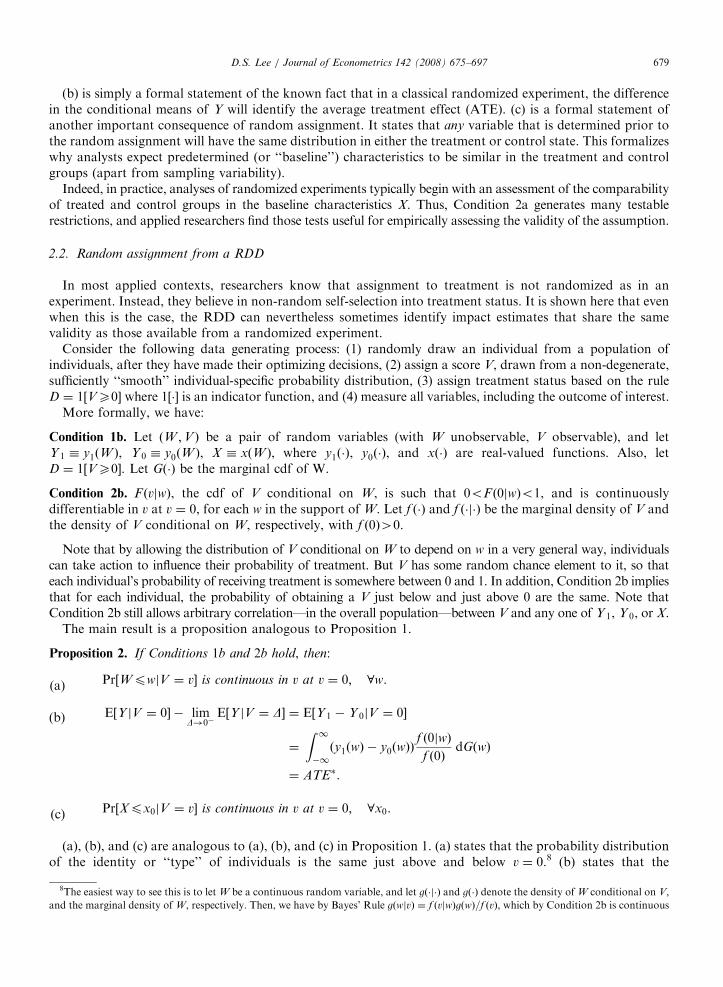
ARTICLE IN PRESSD.S. Lee / Journal of Econometrics 142 (2008) 675–697 679
(b) is simply a formal statement of the known fact that in a classical randomized experiment, the differencein the conditional means of Y will identify the average treatment effect (ATE). (c) is a formal statement ofanother important consequence of random assignment. It states that any variable that is determined prior tothe random assignment will have the same distribution in either the treatment or control state. This formalizeswhy analysts expect predetermined (or ‘‘baseline’’) characteristics to be similar in the treatment and controlgroups (apart from sampling variability).
Indeed, in practice, analyses of randomized experiments typically begin with an assessment of the comparabilityof treated and control groups in the baseline characteristics X. Thus, Condition 2a generates many testablerestrictions, and applied researchers find those tests useful for empirically assessing the validity of the assumption.
2.2. Random assignment from a RDD
In most applied contexts, researchers know that assignment to treatment is not randomized as in anexperiment. Instead, they believe in non-random self-selection into treatment status. It is shown here that evenwhen this is the case, the RDD can nevertheless sometimes identify impact estimates that share the samevalidity as those available from a randomized experiment.
Consider the following data generating process: (1) randomly draw an individual from a population ofindividuals, after they have made their optimizing decisions, (2) assign a score V, drawn from a non-degenerate,sufficiently ‘‘smooth’’ individual-specific probability distribution, (3) assign treatment status based on the ruleD ¼ 1½VX0� where 1½�� is an indicator function, and (4) measure all variables, including the outcome of interest.
More formally, we have:
Condition 1b. Let ðW ;V Þ be a pair of random variables (with W unobservable, V observable), and letY 1 � y1ðW Þ, Y 0 � y0ðW Þ, X � xðW Þ, where y1ð�Þ, y0ð�Þ, and xð�Þ are real-valued functions. Also, letD ¼ 1½VX0�. Let Gð�Þ be the marginal cdf of W.
Condition 2b. F ðvjwÞ, the cdf of V conditional on W, is such that 0oF ð0jwÞo1, and is continuouslydifferentiable in v at v ¼ 0, for each w in the support of W. Let f ð�Þ and f ð�j�Þ be the marginal density of V andthe density of V conditional on W, respectively, with f ð0Þ40.
Note that by allowing the distribution of V conditional on W to depend on w in a very general way, individualscan take action to influence their probability of treatment. But V has some random chance element to it, so thateach individual’s probability of receiving treatment is somewhere between 0 and 1. In addition, Condition 2b impliesthat for each individual, the probability of obtaining a V just below and just above 0 are the same. Note thatCondition 2b still allows arbitrary correlation—in the overall population—between V and any one of Y 1, Y 0, or X.
The main result is a proposition analogous to Proposition 1.
Proposition 2. If Conditions 1b and 2b hold, then:
(a)
8T
and
Pr½WpwjV ¼ v� is continuous in v at v ¼ 0; 8w.
(b)
E½Y jV ¼ 0� � limD!0�E½Y jV ¼ D� ¼ E½Y 1 � Y 0jV ¼ 0�
¼
Z 1�1
ðy1ðwÞ � y0ðwÞÞf ð0jwÞ
f ð0ÞdGðwÞ
¼ ATE�.
(c)
Pr½Xpx0jV ¼ v� is continuous in v at v ¼ 0; 8x0.(a), (b), and (c) are analogous to (a), (b), and (c) in Proposition 1. (a) states that the probability distributionof the identity or ‘‘type’’ of individuals is the same just above and below v ¼ 0.8 (b) states that the
he easiest way to see this is to let W be a continuous random variable, and let gð�j�Þ and gð�Þ denote the density of W conditional on V,
the marginal density of W, respectively. Then, we have by Bayes’ Rule gðwjvÞ ¼ f ðvjwÞgðwÞ=f ðvÞ, which by Condition 2b is continuous

ARTICLE IN PRESSD.S. Lee / Journal of Econometrics 142 (2008) 675–697680
discontinuity in the conditional expectation function identifies an average treatment effect.9 (c), which followsfrom (b), states that all pre-determined characteristics should have the same distribution just below and abovethe threshold. (c) implies that empirical researchers can empirically assess the validity of their RDD, byexamining whether or not, for example, the mean of any pre-determined X conditional on V changesdiscontinuously around 0. If it does, either Condition 1b or 2b must not hold.
It is important to note that ATE� is a particular kind of average treatment effect. It is clearly not theATE for the entire population. Instead, (b) states that it can be interpreted as a weighted ATE: thoseindividuals who are more likely to obtain a draw of V near 0 receive more weight than those who areunlikely to obtain such a draw. Thus, with this treatment-assignment mechanism, it is misleading to statethat the discontinuity gap identifies an average treatment effect ‘‘only for the subpopulation for whomV ¼ 0’’, which is, after all, a measure zero event. It is more accurate to say that it is a weighted averagetreatment effect for the entire population, where the weights are the probability that the individual drawsa V ‘‘near’’ 0.
2.3. Allowing for the impact of V
There are two shortcomings to the treatment-assignment mechanism described by Conditions 1b and 2b.First, it may be too restrictive for some applied contexts. In particular, it assumes that the random draw of V
does not itself have an impact on the outcome—except through its impact on treatment status. That is, while V
is allowed to be correlated with Y 1 or Y 0 in the population, V is not permitted to have an independent causalimpact on Y for a given individual. In a non-experimental setting, this may be unjustifiable. For example, astudent’s score on a scholarship examination might itself have an impact on later-life outcomes, quiteindependently of the receipt of the scholarship.
Second, the counterfactuals Y 1 and Y 0 may not even be well-defined for certain values of V. For example,suppose a merit-based scholarship is awarded to a student solely on the basis of scoring 70% or higher on aparticular examination. What would it mean to receive a test-based scholarship even while scoring 50 on thetest, or to be denied the scholarship even after scoring a 90? In such cases, Y 1 is simply not defined for thosewith Vo0, and Y 0 is not defined for those with ViX0. It may nevertheless be of interest to know the directimpact of winning a test-based scholarship on future academic outcomes.
As another example, suppose we are interested in the causal impact of a Democratic electoral victory in aU.S. Congressional District race on the probability of future Democratic electoral success. We know that aDemocratic electoral victory is a deterministic function of the vote share. Again, the counterfactual notation isawkward, since it makes little sense to conceive of the potential outcome of a Democrat who lost the electionwith 90% of the vote.
To address the limitations above consider the alternative assumption:
Condition 1c. Let ðW ;V Þ be a pair of random variables (with W unobservable, V observable), and letY � yðW ;V Þ, and X � xðW Þ, where for each w, yð�; �Þ is continuous in the second argument except at V ¼ 0,where the function is only continuous from the right. Define the function y�ðwÞ ¼ lime!0 � yðw; eÞ andyþðwÞ ¼ yðw; 0Þ.
yð�; �Þ is a response function relating the outcome to a realization of V. For individual w with realization v ofthe score V, the outcome would be yðw; vÞ. The function yð�; �Þ is simply an analogue to the potential outcomes‘‘function’’ utilized in Conditions 1a and 1b, except that the second argument is a continuous rather than adiscrete variable. For each individual w, there exists an impact of interest, yþðwÞ � y�ðwÞ, and the RD analysisidentifies an average of these impacts.
(footnote continued)
in v at v ¼ 0. It follows thatR w
�1gðzjvÞdz is continuous in v at v ¼ 0. A more general measure-theoretic statement of the proposition that
does not require W to be a continuous random variable, and its proof is available from the author upon request.9Following the preceding footnote, we have E½Y jV ¼ 0� ¼
R1�1
y1ðwÞgðwj0Þdw ¼R1�1
y1ðwÞðf ð0jwÞ=f ð0ÞÞgðwÞdw. Similarly, it follows
that limD!0�E½Y jV ¼ D� ¼R1�1
y0ðwÞðf ð0jwÞ=f ð0ÞÞgðwÞdw, by continuity.

ARTICLE IN PRESSD.S. Lee / Journal of Econometrics 142 (2008) 675–697 681
This leads to:
Proposition 3. If Conditions 1c and 2b hold, then (a) and (c) of Proposition 2 holds, and
(b)
10
poss
follo
avai
E½Y jV ¼ 0� � limD!0�
E½Y jV ¼ D�
¼
Z 1�1
ðyþðwÞ � y�ðwÞÞf ð0jwÞ
f ð0ÞdGðwÞ
¼ ATE��.
So ATE�� is a weighted average of individual-specific discontinuity gaps yþð�Þ � y�ð�Þ where the weights arethe same as in Proposition 2.10
2.4. Self-selection and random chance
The continuity Condition 2b is crucial to the local random assignment results of Propositions 2 and 3. It iseasy to see that if, for a non-trivial fraction of the population, the density of V is discontinuous at the cutoffpoint, then (a), (b), and (c) of Propositions 2 and 3 will generally not be true. Condition 2b is also somewhatintuitive and its plausibility is arguably easier to assess than 1. Indeed, there is a link between Condition 2band the ability of agents to manipulate V, particularly around the discontinuity threshold. When agents canprecisely manipulate their own value of V, it is possible that Condition 2b will not hold, and the RDD couldthen lead to biased impact estimates.
For example, suppose a non-trivial fraction of students taking the examination knew with certainty, foreach question, whether or not their answer was correct—even while taking the exam. If these students caredonly about winning the scholarship per se, and if spending time taking the exam is costly, they would choose toanswer the minimum number of questions correctly (e.g. 70) to obtain the scholarship. In this scenario, clearlythe density of V would be discontinuous at the cutoff point, and thus the use of the RDD would beinappropriate.
Alternatively, suppose for each student, there is an element of chance that determines the score. The studentmay not know the answers to all potential questions, so that at the outset of the examination, which ofthose questions will appear has a random component to it. The student may feel exceptionally sharpthat day or instead may have a bad ‘‘test’’ day, both of which are beyond the control of the student. If thisis a more believable description of the treatment assignment process, then Condition 2b would seemplausible.
One way to formalize the difference between these two different scenarios is to consider that V is the sum oftwo components: V ¼ Z þ e. Z denotes the systematic, or predictable component of V that can depend on theindividuals’ attributes and/or actions (e.g. students’ efforts in studying for the exam), and e is an exogenous,random chance component (e.g. whether the ‘‘right’’ questions appear on the exam, having a good ‘‘testing’’day), with a continuous density. In the first scenario, there was no stochastic component e, since the studentknew exactly whether each of his answers was correct. In the second scenario, however minimally, thecomponent e—random chance—does influence the final score V.
In summary, Propositions 2 and 3 show that localized random assignment can occur even in the presence ofendogenous sorting, as long as agents do not have the ability to sort precisely around the threshold. If theycan, the density of V is likely to be discontinuous, especially if there are benefits to receiving the treatment. Ifthey cannot—perhaps because there is ultimately some unpredictable, and uncontrollable (from the point ofview of the individual) component to V—the continuity of the density may be justifiable.
The easiest way to see this is to let W be a continuous random variable and yð�; �Þ be continuous in both of its arguments, except
ibly in its second argument at V ¼ 0. Then, we have E½Y jV ¼ 0� ¼R1�1
yðw; 0Þgðwj0Þdw ¼R1�1
yþðwÞðf ð0jwÞf ð0ÞÞgðwÞdw. Similarly, it
ws that limD!0�E½Y jV ¼ D� ¼R1�1
y�ðwÞðf ð0jwÞf ð0ÞÞgðwÞdw, by continuity. A more general statement of the proposition and proof is
lable from the author upon request.

ARTICLE IN PRESSD.S. Lee / Journal of Econometrics 142 (2008) 675–697682
2.5. Relation to selection models
The treatment-assignment mechanism described by Conditions 1b (or 1c) and 2b has some generality. Theconditions are implicitly met in typical econometric models for evaluation studies (except for the observabilityof V). For example, consider the reduced-form formulation of Heckman’s (1978) dummy endogenous-variablemodel:
y1 ¼ x1a1 þ dbþ u1,
y�2 ¼ x2a2 þ u2,
d ¼ 1 if y�2X0
¼ 0 if y�2o0, ð2Þ
where y1 is the outcome of interest, d is the treatment indicator, x1 and x2 are exogenous variables and ðu1; u2Þ
are error terms that are typically assumed to be bivariate normal and jointly independent of x1 and x2. Anexclusion restriction typically dictates that x2 contains some variables that do not appear in x1.
Letting V ¼ y�2, and Y 1 ¼ x1a1 þ bþ u, Y 0 ¼ x1a1 þ u, and D ¼ d, it is clear that this conventionalselection model satisfies Conditions 1b and 2b, except that y�2 here is unobservable. In this setting, it is crucialthat the specification (e.g. the choice of variables x1 and x2, the independence assumption, the exclusionrestriction) of the model is correct. Any mis-specification (e.g. missing some variables, correlation between theerrors and x1 and x2, violation of exclusion restriction) will lead to biased estimates of a1, a2, and b.
When, on the other hand, the researcher is fortunate enough to directly observe y�2—as in the RDD—noneof the variables in x1 or x2 are needed for the estimation of b. And it is also unnecessary to assumeindependence of the errors u1; u2. If x1 and x2 are available to the researcher (and insofar as they are known tohave been determined prior to the assignment of d), they can be used to check the validity of the continuityCondition 2b, which drives the local random assignment result. Propositions 2 and 3 imply that this can bedone, for example, by examining the difference E½x1jy
�2 ¼ 0� � limD!0�E½x1jy
�2 ¼ D�. If the local random
assignment result holds, this difference should be zero. The variables x1 and x2 serve another purpose in thissituation. They can be included in a regression analysis to reduce sampling variability in the impact estimates.Local independence implies that the inclusion of those covariates will lead to alternative, consistent estimates,with generally smaller sampling variability. This is analogous to including baseline characteristics in theanalysis of randomized experiments.
It should be noted that this connection between RDD and selection models is not specific to the well-knownparametric version of Eq. (2). The arguments can easily be extended for a more generalized selection modelthat does not assume, for example, the linearity of the indices x1a1 or x2a2, the joint normality of the errors, orthe implied constant treatment effect assumption. Indeed, Condition 1b (or 1c) is perhaps the least restrictivedescription possible for a selection model for the treatment evaluation problem.
3. RDD analysis of the incumbency advantage in the U.S. House
This section applies the ideas developed above to the problem of measuring the electoral advantage ofincumbency in the United States House of Representatives. In the discussion that follows, the ‘‘incumbencyadvantage’’ is defined as the overall causal impact of being the current incumbent party in a district on thevotes obtained in the district’s election. Therefore, the unit of observation is the Congressional district. Therelation between this definition and others commonly used in the political science literature is discussed brieflyin Section 3.5 and in more detail in Appendix B.
3.1. The inference problem in measuring the incumbency advantage
One of the most striking facts of congressional politics in the United States is the consistently high rate ofelectoral success of incumbents, and the electoral advantage of incumbency is one of the most studied aspectsof research on elections to the U.S. House (Gelman and King, 1990). For the United States House of

ARTICLE IN PRESS
0
0.1
0.2
0.3
0.4
0.5
0.6
0.7
0.8
0.9
1
1948 1958 1968 1978 1988 1998
Year
Incumbent Party
Winning Candidate
Runner-up CandidateP
roport
ion W
innin
g E
lect
ion
Fig. 1. Electoral success of U.S. House incumbents: 1948–1998. Note: Calculated from ICPSR study 7757 (ICPSR, 1995). Details in
Appendix A. Incumbent party is the party that won the election in the preceding election in that congressional district. Due to re-
districting on years that end with ‘‘2’’, there are no points on those years. Other series are the fraction of individual candidates in that year,
who win an election in the following period, for both winners and runner-up candidates of that year.
D.S. Lee / Journal of Econometrics 142 (2008) 675–697 683
Representatives, in any given election year, the incumbent party in a given congressional district will likelywin. The solid line in Fig. 1 shows that this re-election rate is about 90% and has been fairly stable over thepast 50 years.11 Well known in the political science literature, the electoral success of the incumbent party isalso reflected in the two-party vote share, which is about 60–70% during the same period.12
As might be expected, incumbent candidates also enjoy a high electoral success rate. Fig. 1 shows that thewinning candidate has typically had an 80 percent chance of both running for re-election and ultimately winning.This is slightly lower, because the probability that an incumbent will be a candidate in the next election is about88%, and the probability of winning, conditional on running for election is about 90%. By contrast, the runner-up candidate typically had a 3% chance of becoming a candidate and winning the next election. The probabilitythat the runner-up even becomes a candidate in the next election is about 20% during this period.
The overwhelming success of House incumbents draws public attention whenever concerns arise thatRepresentatives are using the privileges and resources of office to gain an ‘‘unfair’’ advantage over potentialchallengers. Indeed, the casual observer is tempted to interpret Fig. 1 as evidence that there is an electoraladvantage to incumbency—that winning has a causal influence on the probability that the candidate will runfor office again and eventually win the next election. It is well known, however, that the simple comparison ofincumbent and non-incumbent electoral outcomes does not necessarily represent anything about a trueelectoral advantage of being an incumbent.
As is well-articulated in Erikson (1971), the inference problem involves the possibility of a ‘‘reciprocal causalrelationship’’. Some—potentially all—of the difference is due to a simple selection effect: incumbents are, bydefinition, those politicians who were successful in the previous election. If what makes them successful is somewhatpersistent over time, they should be expected to be somewhat more successful when running for re-election.
3.2. Model
The ideal thought experiment for measuring the incumbency advantage would exogenously change theincumbent party in a district from, for example, Republican to Democrat, while keeping all other factors
11Calculated from data on historical election returns from ICPSR study 7757 (ICPSR, 1995). See Appendix A for details. Note that the
‘‘incumbent party’’ is undefined for years that end with ‘2’ due to decennial congressional re-districting.12See, for example, the overview in Jacobson (1997).

ARTICLE IN PRESSD.S. Lee / Journal of Econometrics 142 (2008) 675–697684
constant. The corresponding increase in Democratic electoral success in the next election would represent theoverall electoral benefit due to being the incumbent party in the district.
There is an RDD inherent in the U.S. Congressional electoral system. Whether or not the Democrats are theincumbent party in a Congressional district is a deterministic function of their vote share in the prior election.
Assuming that there are two parties, consider the following model of Congressional elections:
vi2 ¼ awi1 þ bvi1 þ gdi2 þ ei2,
di2 ¼ 1 vi1X1
2
� �,
f i1ðvjwÞFdensity of vi1 conditional on wi1 Fis continuous in v,
E½ei2jwi1; vi1� ¼ 0, ð3Þ
where vit is the vote share for the Democratic candidate in Congressional district i in election year t. di2 is theindicator variable for whether the Democrats are the incumbent party during the electoral race in year 2. It is adeterministic function of whether the Democrats won election 1. wi1 is a vector of variables that reflect allcharacteristics determined or agents’ choices as of election day in year 1.
The first line in (3) is a standard regression model describing the causal impacts of wi1; vi1, and di2 on vi2. wi1
could represent the partisan make-up of the district, party resources, or the quality of potential nominees. vi1 isalso permitted to impact vi2. For example, a higher vote share may attract more campaign donors, which inturn, could boost the vote share in election year 2. The potentially discontinuous jump in how vi1 impacts vi2 iscaptured by the coefficient g, and is the parameter of interest—the electoral advantage to incumbency.
The main problem is that elements of wi1 may be unobservable to the researcher, so OLS will suffer from anomitted variables bias, since wi1 might be correlated with vi1, and hence with di2. That is, the inherentadvantages the Democrats have in a congressional district (e.g. the degree of liberalness of the constituency,party resources allocated to the district) will naturally be correlated with their electoral success in year 1, andhence will be correlated with whether they are the incumbent party during the electoral race in year 2. This iswhy a simple comparison of electoral success in year 2, between those districts where the Democrats won andlost in year 1, is likely to be biased.
But an RDD can plausibly be used here. Letting W ¼ wi1, V ¼ vi1, and Y ¼ yðW ;V Þ ¼ aW þ bVþ
g � 1 VX12
� �, we have g ¼ y w; 1
2
� �� lime!0þy w; 1
2� e
� �. Conditions 1c and 2b hold, and so Proposition 3
applies.13 Intuitively, conditional on agents’ actions and characteristics as of election day, if there exists arandom chance element (that has a continuous density) to the final vote share vi1, then whether the Democratswin in a closely contested election is would determined as if by a flip of a coin. As a consequence, we canobtain credible estimates of the electoral advantage to incumbency by comparing the average Democratic voteshares in year 2 between districts in which Democrats narrowly won and narrowly lost elections in year 1.
The crucial assumption here is that—even if agents can influence the vote—there is nonetheless a non-trivialrandom chance component to the ultimate vote share, and that conditional on the agents’ choices andcharacteristics, the vote share vi1 has a continuous density. It is plausible that there is at least some random chanceelement to the precise vote share. For example, the weather on election day can influence turnout among voters.
Assuming a continuous density requires that certain kinds of electoral fraud are negligible or non-existent.For example, suppose a non-trivial fraction of Democrats (but no Republicans) had the ability to (1)selectively invalidate ballots cast for their opponents and (2) perfectly predict what the true vote share wouldbe without interfering with the vote counting process. In this scenario, suppose the Democrats followed thefollowing rule: (a) if the ‘‘true’’ vote count would lead to a Republican win, dispute ballots to raise theDemocratic vote share, but (b) if the ‘‘true’’ vote count leads to a Democratic win, do nothing. It is easy to seethat in repeated elections, this rule would lead to a discontinuous density in vi1 right at the 1
2threshold.14
13With the trivial modification that vi2 actually is equal to Y þ ei2, but ei2 has mean zero conditional on V and W, so that
E½vi2jvi1� ¼ E½Y jvi1�.14Note that other ‘‘rules’’ describing fraudulent behavior would nevertheless lead to a continuous density in vi1. For example, suppose
all Democrats had the ability to invalidate ballots during the actual vote counting process. Even if this behavior is rampant, if this ability
stops when 90% of the vote is counted, there is still unpredictability in the vote share tally for the remaining 10% of the ballots. It is
plausible that the probability density for the vote share in the remaining votes is continuous.

ARTICLE IN PRESSD.S. Lee / Journal of Econometrics 142 (2008) 675–697 685
If this kind of fraudulent behavior is important feature of the data, the RDD will lead to invalid inferences;but if it is not, then the RDD is an appropriate design. The important point here is that Proposition 3 (c)implies that the validity of the RDD is empirically testable. That is, if this form of electoral fraud is empiricallyimportant, then all pre-determined (prior to year 1) characteristics (X) should be different between the twosides of the discontinuity threshold; if it is unimportant, then X should have the same distribution on eitherside of the threshold.
3.3. Data issues
Data on U.S. Congressional election returns from 1946 to 1998 are used in the analysis. In order to use allpairs of consecutive elections for the analysis, the dependent variable vi2 is effectively dated from 1948 to 1998,and the independent (score) variable vi1 runs from 1946 to 1996. Due to redistricting every 10 years, and sinceboth lags and leads of the vote share will be used, all cases where the independent variable is from a yearending in ‘0’ and ‘2’ are excluded. Because of possible dependence over time, standard errors are clustered atthe decade–district level.
In virtually all Congressional elections, the strongest two parties will be the Republicans and theDemocrats, but third parties do obtain some small share of the vote. As a result, the cutoff that determines thewinner will not be exactly 50%. To address this, the main vote share variable is the Democratic vote shareminus the vote share of the strongest opponent, which in most cases is a Republican nominee. The Democratwins the election when this variable ‘‘Democratic vote share margin of victory’’ crosses the 0 threshold, andloses the election otherwise.
Incumbency advantage estimates are reported for the Democratic party only. In a strictly two-party system,estimates for the Republican party would be an exact mirror image, with numerically identical results, sinceDemocratic victories and vote shares would have one-to-one correspondences with Republican losses and voteshares.
The incumbency advantage is analyzed at the level of the party at the district level. That is, the analysisfocuses on the advantage to the party from holding the seat, irrespective of the identity of the nominee for theparty. Estimation of the analogous effect for the individual candidate is complicated by selective ‘‘drop-out’’.That is, candidates, whether they win or lose an election, are not compelled to run for (re-)election in thesubsequent period. Thus, even a true randomized experiment would be corrupted by this selective attrition.15
Since the goal is to highlight the parallels between RDD and a randomized experiment, to circumvent thecandidate drop-out problem, the estimates are constructed at the district level; when a candidate runsuncontested, the opposing party is given a vote share of 0.
Four measures of the success of the party in the subsequent election are used: (1) the probability that theparty’s candidate will both become the party’s nominee and win the election, (2) the probability that theparty’s candidate will become the nominee in the election, (3) the party’s vote share (irrespective of who isthe nominee), and (4) the probability that the party wins the seat (irrespective of who is the nominee). The firsttwo outcomes measure the causal impact of a Democratic victory on the political future of the candidate, andthe latter two outcomes measure the causal impact of a Democratic victory on the party’s hold on the districtseat.
Further details on the construction of the data set is provided in Appendix A.
3.4. RDD estimates
Fig. 2a illustrates the RD estimate of the incumbency advantage. It plots the estimated probability of aDemocrat both running in and winning election tþ 1 as a function of the Democratic vote share margin ofvictory in election t. The horizontal axis measures the Democratic vote share minus the vote share of the
15An earlier draft (Lee, 2000) explores what restrictions on strategic interactions between the candidates can be placed to pin down the
incumbency advantage for the candidate for the subpopulation of candidates who would run again whether or not they lose the initial
election. A bounding analysis suggests that most of the incumbency advantage may be due to a ‘‘quality of candidate’’ selection effect,
whereby the effect on drop-out leads to, on average, weaker nominees for the party in the next election.

ARTICLE IN PRESS
0.00
0.10
0.20
0.30
0.40
0.50
0.60
0.70
0.80
0.90
1.00
-0.25 -0.20 -0.15 -0.10 -0.05 0.00 0.05 0.10 0.15 0.20 0.25
Local Average
Logit fit
Democratic Vote Share Margin of Victory, Election t
Pro
bab
ilit
y o
f W
innin
g, E
lect
ion t
+1
0.00
0.50
1.00
1.50
2.00
2.50
3.00
3.50
4.00
4.50
5.00
-0.25 -0.20 -0.15 -0.10 -0.05 0.00 0.05 0.10 0.15 0.20 0.25
Local Average
Polynomial fit
No. of
Pas
t V
icto
ries
as
of
Ele
ctio
n t
Democratic Vote Share Margin of Victory, Election t
Fig. 2. (a) Candidate’s probability of winning election tþ 1, by margin of victory in election t: local averages and parametric fit. (b)
Candidate’s accumulated number of past election victories, by margin of victory in election t: local averages and parametric fit.
D.S. Lee / Journal of Econometrics 142 (2008) 675–697686
Democrats’ strongest opponent (virtually always a Republican). Each point is an average of the indicatorvariable for running in and winning election tþ 1 for each interval, which is 0.005 wide. To the left of thedashed vertical line, the Democratic candidate lost election t; to the right, the Democrat won.
As apparent from the figure, there is a striking discontinuous jump, right at the 0 point. Democrats whobarely win an election are much more likely to run for office and succeed in the next election, compared toDemocrats who barely lose. The causal effect is enormous: about 0.45 in probability. Nowhere else is a jumpapparent, as there is a well-behaved, smooth relationship between the two variables, except at the thresholdthat determines victory or defeat.
Figs. 3a–5a present analogous pictures for the three other electoral outcomes: whether or not the Democratremains the nominee for the party in election tþ 1, the vote share for the Democratic party in the district inelection tþ 1, and whether or not the Democratic party wins the seat in election tþ 1. All figures exhibitsignificant jumps at the threshold. They imply that for the individual Democratic candidate, the causal effectof winning an election on remaining the party’s nominee in the next election is about 0.40 in probability. Theincumbency advantage for the Democratic party appears to be about 7% or 8% of the vote share. In terms ofthe probability that the Democratic party wins the seat in the next election, the effect is about 0.35.

ARTICLE IN PRESS
0.00
0.10
0.20
0.30
0.40
0.50
0.60
0.70
0.80
0.90
1.00
-0.25 -0.20 -0.15 -0.10 -0.05 0.00 0.05 0.10 0.15 0.20 0.25
Local Average
Logit fit
Pro
bab
ilit
y o
f C
andid
acy, E
lect
ion t
+1
0.00
0.50
1.00
1.50
2.00
2.50
3.00
3.50
4.00
4.50
5.00
-0.25 -0.20 -0.15 -0.10 -0.05 0.00 0.05 0.10 0.15 0.20 0.25
Local Average
Polynomial fit
No. of
Pas
t A
ttem
pts
as
of
Ele
ctio
n t
Democratic Vote Share Margin of Victory, Election t
Democratic Vote Share Margin of Victory, Election t
Fig. 3. (a) Candidate’s probability of candidacy in election tþ 1, by margin of victory in election t: local averages and parametric fit. (b)
Candidate’s accumulated number of past election attempts, by margin of victory in election t: local averages and parametric fit.
D.S. Lee / Journal of Econometrics 142 (2008) 675–697 687
In all four figures, there is a positive relationship between the margin of victory and the electoral outcome.For example, as in Fig. 4a, the Democratic vote shares in election t and tþ 1 are positively correlated, both onthe left and right side of the figure. This indicates selection bias; a simple comparison of means of Democraticwinners and losers would yield biased measures of the incumbency advantage. Note also that Figs. 2a, 3a, and5a exhibit important non-linearities: a linear regression specification would hence lead to misleadinginferences.
Table 1 presents evidence consistent with the main implication of Proposition 3: in the limit, there israndomized variation in treatment status. The third to eighth rows of Table 1 are averages of variables that aredetermined before t, and for elections decided by narrower and narrower margins. For example, in the thirdrow, among the districts where Democrats won in election t, the average vote share for the Democrats inelection t� 1 was about 68 percent; about 89 percent of the t� 1 elections had been won by Democrats, as thefourth row shows. The fifth and seventh rows report the average number of terms the Democratic candidateserved, and the average number of elections in which the individual was a nominee for the party, as of electiont. Again, these characteristics are already determined at the time of the election. The sixth and eighth rowsreport the number of terms and number of elections for the Democratic candidates’ strongest opponent. Theserows indicate that where Democrats win in election t, the Democrat appears to be a relatively stronger

ARTICLE IN PRESS
0.30
0.35
0.40
0.45
0.50
0.55
0.60
0.65
0.70
-0.25 -0.20 -0.15 -0.10 -0.05 0.00 0.05 0.10 0.15 0.20 0.25
Local Average
Polynomial fit
Vote
Shar
e, E
lect
ion t
+1
0.30
0.35
0.40
0.45
0.50
0.55
0.60
0.65
0.70
-0.25 -0.20 -0.15 -0.10 -0.05 0.00 0.05 0.10 0.15 0.20 0.25
Local Average
Polynomial fit
Vote
Shar
e, E
lect
ion t
-1
Democratic Vote Share Margin of Victory, Election t
Democratic Vote Share Margin of Victory, Election t
Fig. 4. (a) Democrat party’s vote share in election tþ 1, by margin of victory in election t: local averages and parametric fit. (b)
Democratic party vote share in election t� 1, by margin of victory in election t: local averages and parametric fit.
D.S. Lee / Journal of Econometrics 142 (2008) 675–697688
candidate, and the opposing candidate weaker, compared to districts where the Democrat eventually loseselection t. For each of these rows, the differences become smaller as one examines closer and closer elections—as (c) of Proposition 3 would predict.
These differences persist when the margin of victory is less than 5% of the vote. This is, however, to beexpected: the sample average in a narrow neighborhood of a margin of victory of 5% is in general a biasedestimate of the true conditional expectation function at the 0 threshold when that function has a non-zeroslope. To address this problem, polynomial approximations are used to generate simple estimates of thediscontinuity gap. In particular, the dependent variable is regressed on a fourth-order polynomial in theDemocratic vote share margin of victory, separately for each side of the threshold. The final set of columnsreport the parametric estimates of the expectation function on either side of the discontinuity. Several non-parametric and semi-parametric procedures are also available to estimate the conditional expectation functionat 0. For example, Hahn et al. (2001) suggest local linear regression, and Porter (2003) suggests adaptingRobinson’s (1988) estimator to the RDD.
The final columns in Table 1 show that when the parametric approximation is used, all remainingdifferences between Democratic winners and losers vanish. No differences in the third to eighth rows are

ARTICLE IN PRESS
0.00
0.10
0.20
0.30
0.40
0.50
0.60
0.70
0.80
0.90
1.00
-0.25 -0.20 -0.15 -0.10 -0.05 0.00 0.05 0.10 0.15 0.20 0.25
Local Average
Logit fit
Pro
bab
ilit
y o
f V
icto
ry, E
lect
ion t
+1
Democratic Vote Share Margin of Victory, Election t
0.00
0.10
0.20
0.30
0.40
0.50
0.60
0.70
0.80
0.90
1.00
-0.25 -0.20 -0.15 -0.10 -0.05 0.00 0.05 0.10 0.15 0.20 0.25
Local Average
Logit fit
Pro
bab
ilit
y o
f V
icto
ry, E
lect
ion t
-1
Democratic Vote Share Margin of Victory, Election t
Fig. 5. (a) Democratic party probability victory in election tþ 1, by margin of victory in election t: local averages and parametric fit. (b)
Democratic probability of victory in election t� 1, by margin of victory in election t: local averages and parametric fit.
D.S. Lee / Journal of Econometrics 142 (2008) 675–697 689
statistically significant. These data are consistent with implication (c) of Proposition 3, that all pre-determinedcharacteristics are balanced in a neighborhood of the discontinuity threshold. Figs. 2b, 3b, 4b, and 5b, alsocorroborate this finding. These lower panels examine variables that have already been determined as ofelection t: the average number of terms the candidate has served in Congress, the average number of times hehas been a nominee, as well as electoral outcomes for the party in election t� 1. The figures, which alsosuggest that the fourth order polynomial approximations are adequate, show a smooth relation between eachvariable and the Democratic vote share margin at t, as implied by (c) of Proposition 3.
The only differences in Table 1 that do not vanish completely as one examines closer and closer elections,are the variables in the first two rows of Table 1. Of course, the Democratic vote share or the probability of aDemocratic victory in election tþ 1 is determined after the election t. Thus the discontinuity gap in the finalset of columns represents the RDD estimate of the causal effect of incumbency on those outcomes.
In the analysis of randomized experiments, analysts often include baseline covariates in a regression analysisto reduce sampling variability in the impact estimates. Because the baseline covariates are independent oftreatment status, impact estimates are expected to be somewhat insensitive to the inclusion of these covariates.Table 2 shows this to be true for these data: the results are quite robust to various specifications. Column (1)

ARTICLE IN PRESS
Table 1
Electoral outcomes and pre-determined election characteristics: democratic candidates, winners vs. losers: 1948–1996
Variable All jMarginjo:5 jMarginjo:05 Parametric fit
Winner Loser Winner Loser Winner Loser Winner Loser
Democrat vote share election tþ 1 0.698 0.347 0.629 0.372 0.542 0.446 0.531 0.454
(0.003) (0.003) (0.003) (0.003) (0.006) (0.006) (0.008) (0.008)
[0.179] [0.15] [0.145] [0.124] [0.116] [0.107]
Democrat win prob. election tþ 1 0.909 0.094 0.878 0.100 0.681 0.202 0.611 0.253
(0.004) (0.005) (0.006) (0.006) (0.026) (0.023) (0.039) (0.035)
[0.276] [0.285] [0.315] [0.294] [0.458] [0.396]
Democrat vote share election t� 1 0.681 0.368 0.607 0.391 0.501 0.474 0.477 0.481
(0.003) (0.003) (0.003) (0.003) (0.007) (0.008) (0.009) (0.01)
[0.189] [0.153] [0.152] [0.129] [0.129] [0.133]
Democrat win prob. election t� 1 0.889 0.109 0.842 0.118 0.501 0.365 0.419 0.416
(0.005) (0.006) (0.007) (0.007) (0.027) (0.028) (0.038) (0.039)
[0.31] [0.306] [0.36] [0.317] [0.493] [0.475]
Democrat political experience 3.812 0.261 3.550 0.304 1.658 0.986 1.219 1.183
(0.061) (0.025) (0.074) (0.029) (0.165) (0.124) (0.229) (0.145)
[3.766] [1.293] [3.746] [1.39] [2.969] [2.111]
Opposition political experience 0.245 2.876 0.350 2.808 1.183 1.345 1.424 1.293
(0.018) (0.054) (0.025) (0.057) (0.118) (0.115) (0.131) (0.17)
[1.084] [2.802] [1.262] [2.775] [2.122] [1.949]
Democrat electoral experience 3.945 0.464 3.727 0.527 1.949 1.275 1.485 1.470
(0.061) (0.028) (0.075) (0.032) (0.166) (0.131) (0.23) (0.151)
[3.787] [1.457] [3.773] [1.55] [2.986] [2.224]
Opposition electoral experience 0.400 3.007 0.528 2.943 1.375 1.529 1.624 1.502
(0.019) (0.054) (0.027) (0.058) (0.12) (0.119) (0.132) (0.174)
[1.189] [2.838] [1.357] [2.805] [2.157] [2.022]
Observations 3818 2740 2546 2354 322 288 3818 2740
Note: Details of data processing in Appendix A. Estimated standard errors in parentheses. Standard deviations of variables in brackets.
Data include Democratic candidates (in election t). Democrat vote share and win probability is for the party, regardless of candidate.
Political and Electoral Experience is the accumulated past election victories and election attempts for the candidate in election t,
respectively. The ‘‘opposition’’ party is the party with the highest vote share (other than the Democrats) in election t� 1. Details of
parametric fit in text.
D.S. Lee / Journal of Econometrics 142 (2008) 675–697690
reports the estimated incumbency effect when the vote share is regressed on the victory (in election t) indicator,the quartic in the margin of victory, and their interactions. The estimate should and does exactly match thedifferences in the first row of the last set of columns in Table 1. Column (2) adds to that regression theDemocratic vote share in t� 1 and whether they won in t� 1. The coefficient on the Democratic share in t� 1is statistically significant. Note that the coefficient on victory in t does not change very much. The coefficientalso does not change when the Democrat and opposition political and electoral experience variables areincluded in Columns (3)–(5).
The estimated effect also remains stable when a completely different method of controlling for pre-determined characteristics is utilized. In Column (6), the Democratic vote share tþ 1 is regressed on all pre-determined characteristics (variables in rows three through eight), and the discontinuity jump is estimatedusing the residuals of this initial regression as the outcome variable. The estimated incumbency advantageremains at about 8% of the vote share. This should be expected if treatment is locally independent of all pre-determined characteristics. Since the average of those variables are smooth through the threshold, so shouldbe a linear function of those variables. This principle is demonstrated in Column (7), where the vote share int� 1 is subtracted from the vote share in tþ 1 and the discontinuity jump in that difference is examined.Again, the coefficient remains at about 8%.
Column (8) reports a final specification check of the RDD and estimation procedure. I attempt to estimatethe ‘‘causal effect’’ of winning in election t on the vote share in t� 1. Since we know that the outcome of

ARTICLE IN PRESS
Table 2
Effect of winning an election on subsequent party electoral success: alternative specifications, and refutability test, regression discontinuity
estimates
Dependent variable (1) (2) (3) (4) (5) (6) (7) (8)
Vote share
tþ 1
Vote share
tþ 1
Vote share
tþ 1
Vote share
tþ 1
Vote share
tþ 1
Res. vote share
tþ 1
1st dif. vote share,
tþ 1
Vote share
t� 1
Victory, election t 0.077 0.078 0.077 0.077 0.078 0.081 0.079 �0.002
(0.011) (0.011) (0.011) (0.011) (0.011) (0.014) (0.013) (0.011)
Dem. vote share,
t� 1
– 0.293 – – 0.298 – – –
(0.017) (0.017)
Dem. win, t� 1 – �0.017 – – �0.006 – �0.175 0.240
(0.007) (0.007) (0.009) (0.009)
Dem. political
experience
– – �0.001 – 0.000 – �0.002 0.002
(0.001) (0.003) (0.003) (0.002)
Opp. political
experience
– – 0.001 – 0.000 – �0.008 0.011
(0.001) (0.004) (0.004) (0.003)
Dem. electoral
experience
– – – �0.001 �0.003 – �0.003 0.000
(0.001) (0.003) (0.003) (0.002)
Opp. electoral
experience
– – – 0.001 0.003 – 0.011 �0.011
(0.001) (0.004) (0.004) (0.003)
Note: Details of data processing in Appendix A. N ¼ 6558 in all regressions. Regressions include a fourth order polynomial in the margin
of victory for the Democrats in election t, with all terms interacted with the Victory, election t dummy variable. Political and electoral
experience is defined in notes to Table 2. Column (6) uses as its dependent variable the residuals from a least squares regression on the
Democrat vote share ðtþ 1Þ on all the covariates. Column (7) uses as its dependent variable the Democrat vote share ðtþ 1Þ minus the
Democrat vote share ðt� 1Þ. Column (8) uses as its dependent variable the Democrat vote share ðt� 1Þ. Estimated standard errors (in
parentheses) are consistent with state–district–decade clustered sampling.
D.S. Lee / Journal of Econometrics 142 (2008) 675–697 691
election t cannot possibly causally effect the electoral vote share in t� 1, the estimated impact should be zero.If it significantly departs from zero, this calls into question, some aspect of the identification strategy and/orestimation procedure. The estimated effect is essentially 0, with a fairly small estimated standard error of0.011. All specifications in Table 2 were repeated for the indicator variable for a Democrat victory in tþ 1 asthe dependent variable, and the estimated coefficient was stable across specifications at about 0.38 and itpassed the specification check of Column (8) with a coefficient of �0:005 with a standard error of 0.033.
In summary, the econometric model of election returns outlined in the previous section allows for a greatdeal of non-random selection. The seemingly mild continuity assumption on the distribution of vi1 results inthe strong prediction of local independence of treatment status (Democratic victory) that itself has an‘‘infinite’’ number of testable predictions. The distribution of any variable determined prior to assignmentmust be virtually identical on either side of the discontinuity threshold. The empirical evidence is consistentwith these predictions, suggesting that even though U.S. House elections are non-random selectionmechanisms—where outcomes are influenced by political actors—they also contain randomized experimentsthat can be exploited by RD analysis.16
3.5. Comparison to existing estimates of the incumbency advantage
It is difficult to make a direct comparison between the above RDD estimates and existing estimates of theincumbency advantage in the political science literature. This is because the RDD estimates identify a
16This notion of using ‘‘as good as randomized’’ variation in treatment from close elections has been utilized in Miguel and Zaidi (2003),
Clark (2004), Linden (2004), Lee et al. (2004), DiNardo and Lee (2004).

ARTICLE IN PRESSD.S. Lee / Journal of Econometrics 142 (2008) 675–697692
different, but related concept. The existing literature generally focuses on the concept of an incumbentlegislator advantage, while the RDD approach identifies an overall incumbent party advantage.
Measuring the incumbent legislator advantage answers the following question: From the party’sperspective, what is the electoral gain to having the incumbent legislator run for re-election, relativeto having a new candidate of the same party run in the same district?17 This incumbency advantage isthe electoral success that an incumbent party enjoys if the incumbent runs for re-election, over and above
the electoral outcome that would have occurred if a new nominee for the party had run in the samedistrict.18
By contrast, measuring the incumbent party advantage answers the following question: From the party’sperspective, what is the electoral gain to being the incumbent party in a district, relative to not being theincumbent party? In other words, while the incumbent party’s vote share typically exceeds 50 percent, some ofthe votes would have been gained by the party even if it had not been in control of the seat.
The electoral advantage to being the incumbent party potentially works through a number of differentmechanisms, and includes as a possible mechanism the incumbent legislator advantage. That is, when theDemocratic nominee barely wins an election, it raises the probability that the nominee will run for re-electionas an incumbent legislator. Insofar as there are advantages to being an incumbent legislator as opposed to anew nominee, this will contribute to the overall incumbent party advantage identified by the RDD. Inaddition, the incumbent party advantage includes the gain that would have occurred even if the victoriouscandidate in the first election did not run for re-election.
The interested reader is referred to Appendix B, which explains the difference between the RDD estimate ofthe incumbency advantage and estimates typically found in the political science literature.
4. Conclusion
In one sense, the RDD is no different from all other research designs: causal inferences are only possibleas a direct result of key statistical assumptions about how treatment is assigned to individuals. The keyassumption examined in this paper is the continuity of the density of V for each individual. What makes thetreatment assignment mechanism described in this paper somewhat distinctive is that what appears to be aweak continuity assumption directly leads to very restrictive statistical properties for treatment status.Randomized variation in treatment—independence (local to the threshold)—is perhaps the most restrictiveproperty possible, with potentially an infinite number of testable restrictions, corresponding to the number ofpre-determined characteristics and the number of available moments for each variable. These testablerestrictions are an advantage when seeking to subject the research design to a battery of over-identifyingtests.19
Although the continuity assumption appears to be a weak restriction—particularly since it is implicitlymade in most selection models in econometrics—there are reasons to believe they might be violated whenagents have direct and exact control over the score V. If there are benefits to receiving the treatment, it isnatural to expect those who gain the most to choose their value of V to be above—and potentially justmarginally above—the relevant threshold. Ruling out this kind of behavior appears to be an important part oftheoretically justifying the application of the RDD in any particular context.
17The most precise statement of the counterfactual can be found in Gelman and King (1990), who use ‘‘potential outcomes’’ notation, to
define the ‘‘incumbency advantage’’. They define the incumbency advantage in a district as the difference between ‘‘the proportion of the
vote received by the incumbent legislator in his or her district...’’ and the ‘‘proportion of the vote received by the incumbent party in that
district, if the incumbent legislator does not run...’’.18This notion is also expressed in Alford and Brady (1993), who note that incumbents can incidentally benefit from the party holding the
seat, and that the personal incumbency advantage should be differentiated from the party advantage, and that ‘‘[i]t is this concept of
personal incumbency advantage that most of the incumbency literature, and the related work in the congressional literature, implicitly
turns on.’’ Examples of typical incumbency studies that utilize this concept of incumbency include: Payne (1980), Alford and Hibbing
(1981), Collie (1981), and Garand and Gross (1984). More recently, work by Ansolabehere and Snyder (2001, 2002) and Ansolabehere et
al. (2000) implicitly examine this concept by examining the coefficient on the same incumbency variable defined in Gelman and King
(1990): 1 if a Democrat incumbent seeks re-election, 0 if it is an open seat, and �1 if a Republican seeks re-election.19In addition to testing whether baseline characteristics are similar in the marginal treated and control groups, one can examine if there
is a discontinuity in the marginal distribution of V. See McCrary (2004).
ARTICLE IN PRESSD.S. Lee / Journal of Econometrics 142 (2008) 675–697 693
Acknowledgments
Matthew Butler provided outstanding research assistance. I thank John DiNardo and David Card fornumerous invaluable discussions, and Josh Angrist, Jeff Kling, Jack Porter, Larry Katz, Ted Miguel, and EdGlaeser for detailed comments on an earlier draft. I also thank seminar participants at Harvard, Brown,UIUC, UW-Madison and Berkeley, and Jim Robinson, and Andrew Gelman for their additional commentsand suggestions.
Appendix A. Description of data
The data used for this analysis are based on the candidate-level Congressional election returns for the U.S.,from ICPSR study 7757, ‘‘Candidate and Constituency Statistics of Elections in the United States,1788–1990’’ (ICPSR, 1995).
The data were initially checked for internal consistencies (e.g. candidates’ vote totals not equalling reportedtotal vote cast), and corrected using published and official sources (Congressional Quarterly, 1997 and theUnited States House of Representatives Office of the Clerk’s Web Page). Election returns from 1992–1998were taken from the United States House of Representatives Office of the Clerk’s Web Page, and appended tothese data. Various states (e.g. Arkansas, Louisiana, Florida, and Oklahoma) have laws that do not requirethe reporting of candidate vote totals if the candidate ran unopposed. If they are the only candidate in thedistrict, they were assigned a vote share of 1. Other individual missing vote totals were replaced with validtotals from published and official sources. Individuals with more than one observation in a district year (e.g.separate Liberal and Democrat vote totals for the same person in New York and Connecticut) were given thetotal of the votes, and were assigned to the party that gave the candidate the most votes. The name of thecandidate was parsed into last name, first name, and middle names, and suffixes such as ‘‘Jr., Sr., II, III, etc.’’
Since the exact spelling of the name differs across years, the following algorithm was used to create a uniqueidentifier for an individual that could match the person over time. Individuals were first matched on state, firstfive characters of the last name, and first initial of the first name. The second layer of the matching processisolates those with a suffix such as Jr. or Sr., and small number of cases were hand-modified using publishedand official sources. This algorithm was checked by drawing a random sample of 100 election-year-candidateobservations from the original sample, tracking down every separate election the individual ran in (usingpublished and official sources; this expanded the random sample to 517 election-year-candidate observations),and asking how well the automatic algorithm performed. The fraction of observations from this ‘‘truth’’sample that matched with the processed data was 0.982. The fraction of the processed data for which there wasa ‘‘true’’ match was 0.992. Many different algorithms were tried, but the algorithm above performed bestbased on the random sample.
Throughout the sample period (1946–1998), in about 3% of the total possible number of elections (based onthe number of seats in the House in each year), no candidate was reported for the election. I impute themissing values using the following algorithm. Assign the state–year average electoral outcome; if still missing,assign the state–decade average electoral outcome.
Two main data sets are constructed for the analysis. For all analysis at the Congressional level, I keep allyears that do not end in ‘0’ or ‘2’. This is because, strictly speaking, Congressional districts cannot be matchedbetween those years, due to decennial redistricting, and so in those years, the previous or next electoraloutcome is undefined. The final data set has 6558 observations. For the analysis at the individual candidatelevel, one can use more years, because, despite redistricting, it is still possible to know if a candidate ran insome election, as well as the outcome. This larger dataset has 9674 Democrat observations.
For the sake of conciseness, the empirical analysis in the paper focuses on observations for Democrats only.This is done to avoid the ‘‘double-counting’’ of observations, since in a largely two-party context, a winningDemocrat will, by construction, produce a losing Republican in that district and vice versa. (It is unattractiveto compare a close winner to the closer loser in the same district.) In reality, there are third-party candidates,so a parallel analysis done by focusing on Republican candidates will not give a literal mirror image of theresults. However, since third-party candidates tend not to be important in the U.S. context, it turns out that allof the results are qualitatively the same, and are available from the author upon request.
ARTICLE IN PRESSD.S. Lee / Journal of Econometrics 142 (2008) 675–697694
Appendix B. Comparison of RDD and other estimates of the incumbency advantage
Reviews of the existing methodological literature in Gelman and King (1990), Alford and Brady (1993), andJacobson (1997) suggest that most of the research on incumbency are variants of three general approaches—the ‘‘sophomore surge’’, the ‘‘retirement slump’’, and the Gelman–King index (1990).20 Figs. B1a and billustrate the differences between these three approaches and the regression discontinuity strategy employed inthis paper. They also clearly show that the three commonly used approaches to measuring the ‘‘incumbencyadvantage’’ are estimating an incumbent legislator advantage as opposed to an incumbent party advantage. TheRDD is ideally suited for estimating the latter incumbency advantage.
Fig. B1a illustrates the idea behind the ‘‘sophomore surge’’. The solid line shows a hypothetical relationshipbetween the average two-party Democratic vote share in period 2—V 2—as a function of the Democratic voteshare in period 1, V1. In addition, the dotted line just below the solid line on the right side of the graphrepresents the average V2 as a function of V1, for the sub-sample of elections that were won by first-timeDemocrats in period 1.21 The idea behind the sophomore surge is to subtract from the average V2 for allDemocratic first-time incumbents (V 2), an amount that represents the strength of the party in those districtsapart from any incumbent legislator advantage. The ‘‘sophomore surge’’ approach subtracts off V 1, theaverage V 1 for those same Democratic first-time incumbents.
Fig. B1b illustrates how the ‘‘retirement slump’’ is a parallel measure to the ‘‘sophomore surge’’. In thisfigure, the dashed line below the solid line represents the average V 2 as a function of V 1, for those districts thatwill have open seats as of period 2. In other words, it is the relationship for those districts in which theDemocratic incumbent retires and does not seek re-election in period 2. Here, the idea is to subtract from theaverage vote share gained by the retiring Democratic incumbents (V 1), an amount that reflects the strength ofthe party. The ‘‘retirement slump’’ approach subtracts off V 2, the average V2 for the incoming Democraticcandidate in those districts.
Fig. B1b also illustrates Gelman and King’s approach to measuring incumbency advantage. The dotted lineabove the solid line is the average V2, as a function of V1, for those districts in which the Democraticincumbent is seeking re-election. The idea behind their approach is to subtract from the average vote share V 2
gained by incumbents seeking re-election, an amount that reflects how the party would perform if a newcandidate ran for the party, while controlling for the lagged vote share V 1. Thus, the gap between the paralleldashed and dotted lines in Fig. B1b represent the incumbent legislator advantage measured by theGelman–King index (c).22
Finally, Figs. B1a and b illustrate that the approach of the RDD isolates a different aspect of theincumbency advantage—the incumbent party advantage. The idea is to make a comparison of theelectoral performance in period 2 of the Democratic party between districts that were barely won (say,by 0.1% of the vote) and districts that were barely lost by the Democratic party in period 1. Thus theRD estimate (b) is depicted by the discontinuous jumps in the solid lines at the 0.50 threshold in Figs. B1aand b.23
The figures show that the discontinuity gap directly addresses the counterfactual question that is at the heartof measuring the incumbent party advantage: How would the Democratic party have performed in period 2, had
they not held the seat (i.e. had the Democrats lost the election in period 1)? The best way to estimate thatquantity is to examine elections where the Democrats just barely missed being the incumbent party for theelection in period 2—the point on the solid line just to the left of the 0.50 threshold.
20See Gelman and King (1990) for a concise review of existing methods as of 1990. More recently, Levitt and Wolfram (1997) use a
‘‘modified sophomore surge’’ approach and Cox and Katz (1996) use a specification ‘‘adapted from Gelman and King (1990)’’.21In principle, a ‘‘mirror-image’’ line exists for the Republican first-time incumbents. But I omit the line to make the graph clearer. Also,
note that in this graph, to simplify exposition, I am assuming that all first-time incumbents seek re-election. The basic ideas hold when
relaxing this assumption, but the notation is slightly more cumbersome.22Again, the mirror-image dotted and dashed lines for Republicans are ignored to make the exposition clearer in the graph.23While it is tempting to equate b here to b2 in equation (6) of Gelman and King (1990), this would be incorrect, because Gelman and
King also include their key variable of interest, I2, in the specification. (If I2 were not included, then b2 would be comparable to b here,
provided that the underlying regression function is linear).
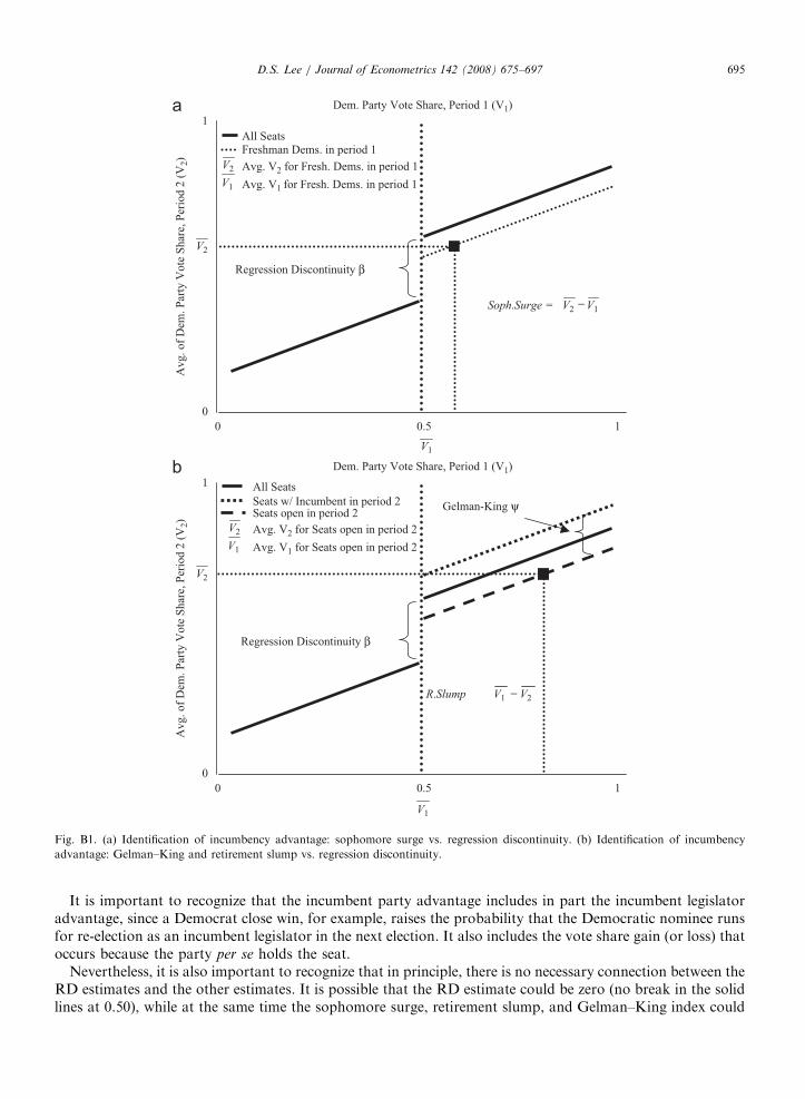
ARTICLE IN PRESS
Dem. Party Vote Share, Period 1 (V1)
Avg. of
Dem
. P
arty
Vote
Shar
e, P
erio
d 2
(V
2)
0
0
0.5 1
1
Regression Discontinuity β
V1
V2
V1V2Soph.Surge =
0
0
0.5 1
1
Regression Discontinuity β
V1
V2
V2V1R.Slump
Gelman-King ψ
All Seats
Freshman Dems. in period 1
Avg. V2 for Fresh. Dems. in period 1
Avg. V1 for Fresh. Dems. in period 1
V2
V1
V2
All Seats
Seats w/ Incumbent in period 2 Seats open in period 2
Avg. V2 for Seats open in period 2
Avg. V1 for Seats open in period 2V1
Dem. Party Vote Share, Period 1 (V1)
Avg. of
Dem
. P
arty
Vote
Shar
e, P
erio
d 2
(V
2)
−
−
Fig. B1. (a) Identification of incumbency advantage: sophomore surge vs. regression discontinuity. (b) Identification of incumbency
advantage: Gelman–King and retirement slump vs. regression discontinuity.
D.S. Lee / Journal of Econometrics 142 (2008) 675–697 695
It is important to recognize that the incumbent party advantage includes in part the incumbent legislatoradvantage, since a Democrat close win, for example, raises the probability that the Democratic nominee runsfor re-election as an incumbent legislator in the next election. It also includes the vote share gain (or loss) thatoccurs because the party per se holds the seat.
Nevertheless, it is also important to recognize that in principle, there is no necessary connection between theRD estimates and the other estimates. It is possible that the RD estimate could be zero (no break in the solidlines at 0.50), while at the same time the sophomore surge, retirement slump, and Gelman–King index could

ARTICLE IN PRESSD.S. Lee / Journal of Econometrics 142 (2008) 675–697696
be significant. Alternatively, in principle, there could be a large estimate of b, while at the same time the othermeasures could be zero.
A final important point is that the sophomore surge relies upon situations where either an incumbent isdefeated or a seat is thrown open, and the retirement slump, and Gelman–King index relies upon situationswhere seats are thrown open by an incumbent that does not seek re-election. In principle, for any year in whichevery incumbent becomes the nominee in a re-election bid (and ignoring redistricting years) it would beimpossible to estimate any of those three measures; the dotted and dashed lines in Figs. B1a and b would notexist. In this case, the only incumbency advantage concept that could be measured would be the incumbentparty advantage identified by the RDD.
References
Alford, J.R., Brady, D.W., 1993. Personal and partisan advantage in U.S. congressional elections. In: Dodd, L.C., Oppenheimer, B.I.
(Eds.), Congress Reconsidered, fifth ed. CQ Press, Washington, DC.
Alford, J.R., Hibbing, J.R., 1981. Increased incumbency advantage in the house. Journal of Politics 43, 1042–1061.
Angrist, J.D., Lavy, V., 1998. Using maimondies’ rule to estimate the effect of class size on scholastic achievement. Quarterly Journal of
Economics 114, 533–575.
Ansolabehere, S., Snyder, J.M., 2001. The Incumbency Advantage in U.S. Elections: An Analysis of State and Federal Offices, 1942–2000.
MIT manuscript, June 2001.
Ansolabehere, S., Snyder, J.M., 2002. Using Term Limits to Estimate Incumbency Advantages When Officeholders Retire Strategically.
MIT manuscript, January 2002.
Ansolabehere, S., Snyder, J.M., Stewart, C., 2000. Old voters, new voters, and the personal vote: using redistricting to measure the
incumbency advantage. American Journal of Political Science 44, 17–34.
Clark, D., 2004. Politics, Markets and Schools: Quasi-Experimental Evidence on the Impact of Autonomy and Competition from a Truly
Reveloutionary UK Reform. Manuscript, November 2004.
Collie, M.P., 1981. Incumbency, electoral safety, and turnover in the house of representatives 1952–1976. American Political Science
Review 75, 119–131.
Congressional Quarterly, 1997. Congressional Elections: 1946–1996.
Cox, G., Katz, J., 1996. Why did the incumbency advantage grow. American Journal of Political Science 40, 478–497.
DiNardo, J., Lee, D.S., 2004. Economic impacts of new unionization on private sector employers: 1984–2001. Quarterly Journal of
Economics 119, 1383–1442.
Erikson, R.S., 1971. The advantage of incumbency in congressional elections. Polity 3, 395–405.
Garand, J.C., Gross, D.A., 1984. Change in the vote margins for congressional candidates: a specification of the historical trends.
American Political Science Review 78, 17–30.
Gelman, A., King, G., 1990. Estimating incumbency advantage without bias. American Journal of Political Science 34, 1142–1164.
Hahn, J., Todd, P., van der Klaauw, W., 2001. Identification and estimation of treatment effects with a regression-discontinuity design.
Econometrica 69, 201–209.
Heckman, J., 1978. Dummy endogenous variables in a simultaneous equation system. Econometrica 46 (4), 931–959.
Inter-university Consortium for Political and Social Research (ICPSR), 1995. Candidate and Constituency Statistics of Elections in the
United States, 1788–1990 Computer File 5th ICPSR ed. Ann Arbor, MI: Inter-university Consortium for Political and Social
Research, producer and distributor, 1995.
Jacobson, G.C., 1997. The Politics of Congressional Elections. Longman, Menlo Park, California.
Lee, D.S., 2000. Is there really an electoral advantage to incumbency? Evidence from close elections to the United States House of
Representatives. Harvard University manuscript, April 2000.
Lee, D.S., Moretti, E., Butler, M.J., 2004. Do voters affect or elect policies? evidence from the U.S. House. Quarterly Journal of
Economics 119, 807–860.
Levitt, S.D., Wolfram, C.D., 1997. Decomposing the sources of incumbency advantage in the U.S. House. Legislative Studies Quarterly
22, 45–60.
Linden, L., 2004. Are incumbents really advantaged? The preference for non-incumbents in indian national elections. Columbia University
manuscript, January 2004.
Martorell, F., 2004. Do graduation exams matter? A regression-discontinuity analysis of the impact of failing the exit exam on high school
and post-high school outcomes. UC Berkeley manuscript, September 2004.
Matsudaira, J.D., 2004. Sinking or swimming? Evaluating the impact of english immersion vs. bilingual education on student achievement.
University of Michigan manuscript, October 2004.
McCrary, J., 2004. Testing for manipulation of the running variable in the regression discontinuity design. University of Michigan
manuscript.
Miguel, E., Zaidi, F., 2003. Do politicians reward their supporters? Public spending and incumbency advantage in Ghana. UC Berkeley
manuscript.
Payne, J.L., 1980. The personal electoral advantage of house incumbents. American Politics Quarterly 8, 375–398.

ARTICLE IN PRESSD.S. Lee / Journal of Econometrics 142 (2008) 675–697 697
Porter, J., 2003. Estimation in the regression discontinuity model. Harvard University manuscript, May 2003.
Robinson, P., 1988. Root-n-consistent semiparametric regression. Econometrica 56, 931–954.
Thistlethwaite, D., Campbell, D., 1960. Regression-discontinuity analysis: an alternative to the ex post facto experiment. Journal of
Educational Psychology 51, 309–317.
van der Klaauw, W., 2002. Estimating the effect of financial aid offers on college enrollment: a regression–discontinuity approach.
International Economic Review 43 (4).