Rank-one Perturbation of Weighted Shifts on a Directed Tree:

Partial Normality and Weak Hyponormality

George R. Exner, Il Bong Jung, Eun Young Lee and Minjung Seo∗†

Abstract

A special rank-one perturbation St,n of a weighted shift on a directed tree isconstructed. Partial normality and weak hyponormality (including quasinormal-ity, p-hyponormality, p-paranormality, absolute-p-paranormality and A(p)-class)of St,n are characterized.

1. Introduction

Let H be a separable, infinite dimensional, complex Hilbert space and let B(H) bethe algebra of all bounded linear operators on H. For nonzero vectors u and v in H weshall write u⊗v for the rank-one operator in B(H) defined by (u⊗ v) (x) = 〈x, v〉u, x ∈H. For X, Y ∈ B(H), we denote by [X, Y ] = XY − Y X the commutator of X and Y .An operator T ∈ B(H) is normal if [T ∗, T ] = 0, subnormal if it is (unitarily equivalentto) the restriction of a normal operator to an invariant subspace, and hyponormalif [T ∗, T ] ≥ 0. An operator T ∈ B(H) is said to be p-hyponormal (0 < p < ∞)if (T ∗T )p ≥ (TT ∗)p. In particular, if p = 1

2, then T is said to be semi-hyponormal

([26]). And T ∈ B(H) is ∞-hyponormal if T is p-hyponormal for all p ∈ (0,∞).According to the Lowner-Heinz inequality ([16],[26]), every q-hyponormal operator isp-hyponormal for p ≤ q. Recall that an operator T ∈ B(H) has the unique polar

decomposition T = U |T |, where |T | = (T ∗T )12 and U is a partial isometry satisfying

kerU = ker |T | = kerT and kerU∗ = kerT ∗. An operator T is absolute-p-paranormal if‖|T |pTx‖ ≥ ‖Tx‖p+1 for all unit vectors x inH. Note that every absolute-q-paranormaloperator is absolute-p-paranormal for q ≤ p ([16]). And for each p > 0, an operatorT is p-paranormal if ‖ |T |p U |T |p x‖ ≥ ‖ |T |p x‖2 for all unit vectors x in H. Everyq-paranormal operator is p-paranormal for q ≤ p. Note that absolute-1-paranormalityand 1-paranormality coincide; we call this property paranormality for simplicity. An

operator T is A(p)-class if (T ∗ |T |2p T )1p+1 ≥ |T |2. There are relations among the classes

of operators mentioned above as follows:

∗2010 Mathematics Subject Classification. Primary 47B20, 05C20, 47B37; Secondary 47A55,47A50.†Key words and phrases: rank-one perturbation, weighted shifts on directed trees, p-hyponormal

operators, absolute-p-paranormal operators, p-paranormal operators, A(p)-class operators.

1

• subnormal ⇒ p-hyponormal ⇒ p-paranormal ⇒ absolute-p-paranormal (when0 < p < 1);

• subnormal ⇒ p-hyponormal ⇒ absolute-p-paranormal ⇒ p-paranormal (whenp > 1);

• A(p)-class ⇒ absolute-p-paranormal (when p > 0).

The operator classes between subnormal and normaloid have been studied for morethan 40 years (see [2],[3],[8],[16],[26]). Also, some operator models have been studiedto detect those classes. For example, some block matrix operators induced by compo-sition operators on discrete measure spaces were considered to exemplify some classesabove (cf. [6],[7],[22],[23]). In [19] the notion of weighted shifts Sλ on directed trees wasintroduced and has been developed well for recently for several years. But this operatorSλ is not enough to differentiate the above classes; for example, Sλ is p-paranormal ifand only if Sλ is absolute-p-paranormal (cf. Section 4). But a rank-one perturbationSt,n of Sλ which will be defined below (Section 2.2) is a good operator model to de-tect gaps of weak hyponormalities. In fact, the weighted shifts on directed trees havebeen discussed as a special model of weighted adjacency operators on directed graphswhich generalizes Fujii-Sasaoka-Watatani’s operator models; see [9],[12],[13],[14],[15]for related results. Note that the rank-one perturbations of a bounded (unbounded)operator can be applied to several related areas in mathematical physics as well as op-erator theory ([5],[10],[11],[21],[24]). In this paper we characterize the quasinormality,p-hyponormality, p-paranormality, absolute-p-paranormality and A(p)-class of opera-tors St,n which exemplify some operator gaps between normal and nomaloid operators.

The paper consists of five sections. In Section 2, we assemble some useful ob-servations and recall some terminology and notation concerning weighted shifts ondirected trees. And also we construct the rank-one perturbation St,n of the weightedshift Sλ on a certain directed tree T2,κ. In Section 3, we characterize p-hyponormalityof St,n and discuss some related remarks. In Section 4, we also characterize absolute-p-paranormality, p-paranormality and A(p)-class property of St,n. In Section 5, weconsider some related examples.

Throughout this paper we write C[R,R+,Z+,N, resp.] for the set of complex num-bers [real numbers, positive real numbers, nonnegative integers, positive integers, resp.].Some of the calculations in this paper were obtained through computer experimentsusing the software tool Mathematica [25].

2. Preliminaries and notations

2.1. Some basic observations. In what follows we will frequently have use forcertain elementary observations which we record here and use with little or no furthercomment. First, if a, b and p are positive real numbers, then abp−(p+1)spa+psp+1 ≥ 0for all s ≥ 0 if and only if b ≥ a. Second, it is the standard Nested Determinant test([4, p.213]) that a real symmetric matrix M is non-negative if the determinants of its

2

principal submatrices are positive and det(M)≥ 0. For a two-by-two real symmetricmatrix A, A is positive semi-definite if and only if both its diagonal entries are non-negative and det(A)≥ 0.

Third, we will frequently have occasion to find powers q of a real symmetric matrix(a bb c

), which we do as usual by transforming to a diagonal matrix of eigenvalues

using the associated eigenvectors. The eigenvalues are

1

2

((a+ c)∓

√(a+ c)2 − 4(ac− b2)

).

We will frequently call these names such as ρ1 and ρ2, with associated eigenvectors e1and e2, and abbreviate the square root term by some name such as γ. If we express theeigenvectors as e1 = ((a− ρ2)/b, 1)T and e2 = ((a− ρ1)/b, 1)T , the resulting expressionfor Aq, which we call form 1, is(

(ρ2−a)ρq1−(ρ1−a)ρq2

γ

b(ρq2−ρq1)

γb(ρq2−ρ

q1)

γ

(ρ2−a)ρq2−(ρ1−a)ρq1

γ

).

If instead we express the eigenvectors as e1 = ((ρ1− c)/b, 1)T and e2 = ((ρ2− c)/b, 1)T ,the resulting expression for Aq, which we call form 2, is(

(ρ2−c)ρq2−(ρ1−c)ρq1

γ

b(ρq2−ρq1)

γb(ρq2−ρ

q1)

γ

(ρ2−c)ρq1−(ρ1−c)ρq2

γ

).

When we apply this process we will indicate the form, the eigenvalues, and the squareroot term for the reader’s convenience.

2.2. Directed trees. In this section we recall some definitions and terminologyin graph theory which will be used in this paper ([19],[20]). First of all, we look atsome basic notions of graph theory. A pair G = (V,E) is a directed graph if V is anonempty set and E is a subset of V × V \ (v, v) | v ∈ V . We set

E = u, v ⊆ V | (u, v) ∈ E or (v, u) ∈ E.

An element of V is called a vertex of G, a member of E is called an edge of G, and amember of E is called an undirected edge. A directed graph G is said to be connectedif for any two distinct vertices u and v of G, there exists a finite sequence v1, · · · , vnof vertices of G(n ≥ 2) such that u = v1, vj, vj+1 ∈ E for all j = 1, · · · , n − 1, andvn = v. Such a sequence will be called an undirected path joining u and v. For u ∈ V ,put

Chi(u) = v ∈ V | (u, v) ∈ E.

An element of Chi(u) is called a child of u. If, for a given vertex u ∈ V , there exists aunique vertex v ∈ V such that (v, u) ∈ E, then we say that u has a parent v and write

3

par(u) for v. A vertex v of G is called a root of G, or briefly v ∈ Root(G), if there isno vertex u of G such that (u, v) is an edge of G. If Root(G) is a one-element set, thenits unique element is denoted by root(G), or simply by root if this causes no ambiguity.We write V = V \Root(G). A finite sequence ujnj=1 (n ≥ 2) of distinct vertices issaid to be a circuit of G if (uj, uj+1) ∈ E for all j = 1, · · · , n− 1, and (un, u1) ∈ E. Adirected graph T is a directed tree if T is connected, has no circuits and each vertexin v ∈ V has a parent. From now on, T = (V,E) is assumed to be a directed tree.Note that `2(V ) is the Hilbert space of all square summable complex functions on Vwith the standard inner product

〈f, g〉 =∑u∈V

f(u)g(u), f, g ∈ `2(V ).

For u ∈ V , we define eu ∈ `2(V ) by

eu(v) =

1 if u = v,0 otherwise.

Then the set euu∈V is an orthonormal basis of `2(V ). For λ = λvv∈V ⊂ C, wedefine the operator Sλ on `2(V ) with the domain D(Sλ) such that

D(Sλ) = f ∈ `2(V ) :∑u∈V

∑v∈Chi(u)

|λv|2 |f(u)|2 <∞,

Sλf = ΛT f, f ∈ D(Sλ),

where ΛT is the mapping defined on functions f : V → C by

(ΛT f)(v) =

λv · f(par(v)) if v ∈ V ,0 if v = root.

In this case the operator Sλ is called a weighted shift on the directed tree T withweights λvv∈V . In particular, if Sλ ∈ B(H), then

Sλeu =∑

v∈Chi(u)

λvev

(cf. [19, Prop. 3.1.3]) and

S∗λeu =

λuepar(u) if u ∈ V ,0 if u is root;

these formulas are used frequently in this paper (cf. [19, Prop. 3.4.1]). Recall that Sλis bounded if and only if supu∈V

∑v∈Chi(u) |λv|2 < ∞. In this paper we only consider

the operators Sλ in B(`2(V )). We deal with weighted shifts associated to the following

4

models and this model is closely related to the subnormality of weighted shifts ondirected trees (cf. [19]).

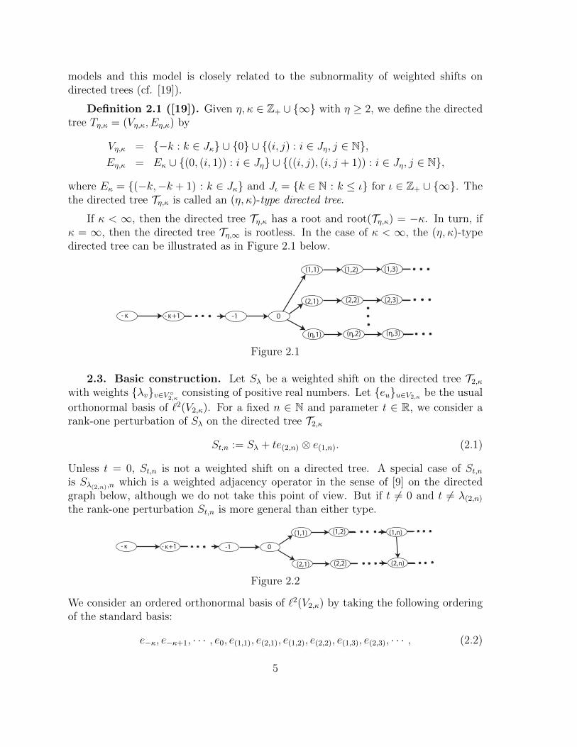
Definition 2.1 ([19]). Given η, κ ∈ Z+ ∪ ∞ with η ≥ 2, we define the directedtree Tη,κ = (Vη,κ, Eη,κ) by

Vη,κ = −k : k ∈ Jκ ∪ 0 ∪ (i, j) : i ∈ Jη, j ∈ N,Eη,κ = Eκ ∪ (0, (i, 1)) : i ∈ Jη ∪ ((i, j), (i, j + 1)) : i ∈ Jη, j ∈ N,

where Eκ = (−k,−k + 1) : k ∈ Jκ and Jι = k ∈ N : k ≤ ι for ι ∈ Z+ ∪ ∞. Thethe directed tree Tη,κ is called an (η, κ)-type directed tree.

If κ < ∞, then the directed tree Tη,κ has a root and root(Tη,κ) = −κ. In turn, ifκ = ∞, then the directed tree Tη,∞ is rootless. In the case of κ < ∞, the (η, κ)-typedirected tree can be illustrated as in Figure 2.1 below.

- κ - κ+1 -1 0

(1,1) (1,2) (1,3)

(2,1) (2,2) (2,3)

(η,1) (η,2) (η,3)

Figure 2.1

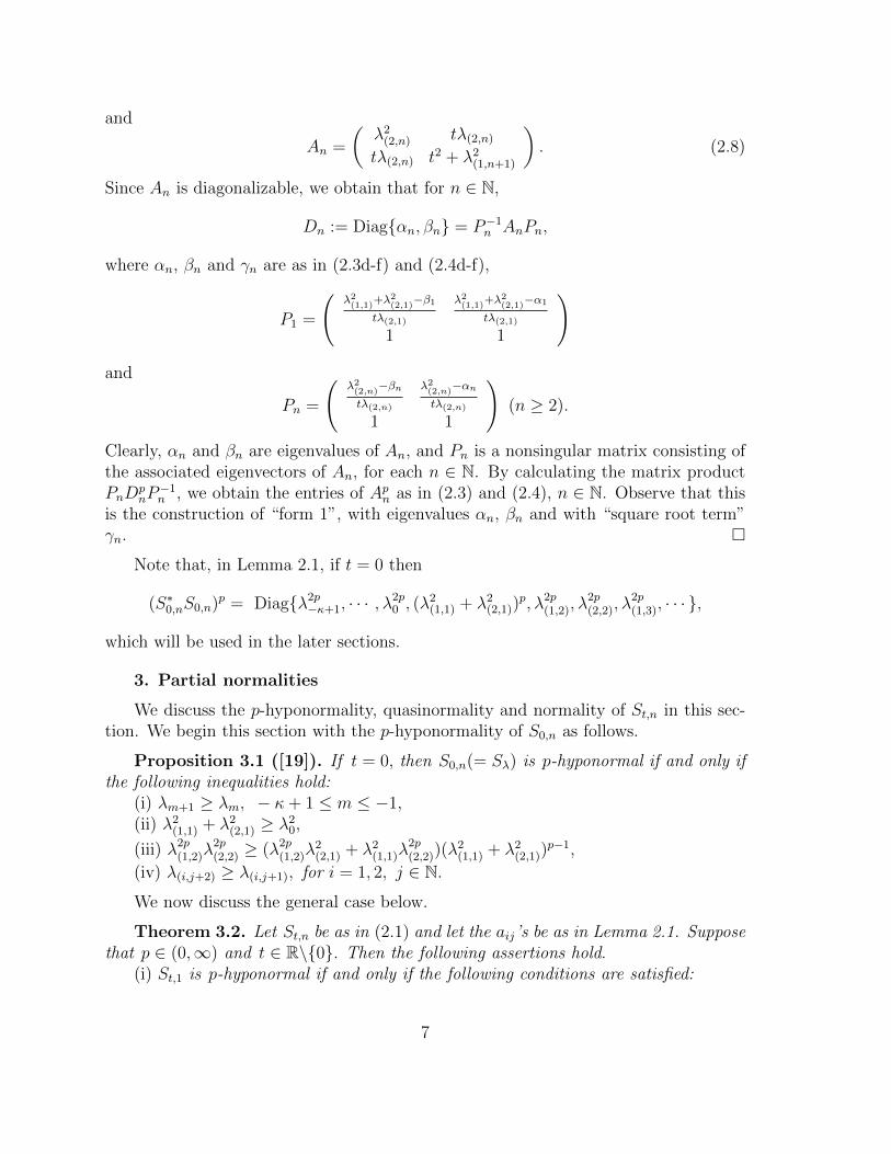
2.3. Basic construction. Let Sλ be a weighted shift on the directed tree T2,κwith weights λvv∈V

2,κconsisting of positive real numbers. Let euu∈V2,κ be the usual

orthonormal basis of `2(V2,κ). For a fixed n ∈ N and parameter t ∈ R, we consider arank-one perturbation of Sλ on the directed tree T2,κ

St,n := Sλ + te(2,n) ⊗ e(1,n). (2.1)

Unless t = 0, St,n is not a weighted shift on a directed tree. A special case of St,nis Sλ(2,n),n which is a weighted adjacency operator in the sense of [9] on the directedgraph below, although we do not take this point of view. But if t 6= 0 and t 6= λ(2,n)the rank-one perturbation St,n is more general than either type.

- κ - κ+1 -1 0

(1,1) (1,2)

(2,1) (2,2)

(1,n)

(2,n)

Figure 2.2

We consider an ordered orthonormal basis of `2(V2,κ) by taking the following orderingof the standard basis:

e−κ, e−κ+1, · · · , e0, e(1,1), e(2,1), e(1,2), e(2,2), e(1,3), e(2,3), · · · , (2.2)

5

and consider throughout this paper the matrices corresponding to operators St,n relativeto the ordered orthonormal basis in (2.2).

First, we begin with the following computational lemma.

Lemma 2.1. Let St,n be as in (2.1). Suppose that p ∈ (0,∞). If t 6= 0, then thefollowing assertions hold :

(i) (S∗t,1St,1)p = Diagλ2p−κ+1, · · · , λ

2p−1, λ

2p0 , A

p1, λ

2p(2,2), λ

2p(1,3), λ

2p(2,3), λ

2p(1,4), · · · ,

where Ap1 is unitarily equivalent to a 2× 2 matrix (aij(1, p))1≤i,j≤2 with

a11(1, p) = (β1 − λ2(1,1) − λ2(2,1))αp1 + (λ2(1,1) + λ2(2,1) − α1)β

p1/γ1, (2.3a)

a12(1, p) = a21(1, p) = tλ(2,1)(βp1 − α

p1)/γ1, (2.3b)

a22(1, p) = (λ2(1,1) + λ2(2,1) − α1)αp1 + (β1 − λ2(1,1) − λ2(2,1))β

p1/γ1, (2.3c)

α1 = (t2 + λ2(1,1) + λ2(2,1) + λ2(1,2) − γ1)/2, (2.3d)

β1 = (t2 + λ2(1,1) + λ2(2,1) + λ2(1,2) + γ1)/2, (2.3e)

γ1 = [(t2 + λ2(1,1) + λ2(1,2) + λ2(2,1))2 − 4λ2(1,2)λ2(2,1) + λ2(1,1)(t

2 + λ2(1,2))]1/2, (2.3f)

(ii) for n ≥ 2,

(S∗t,nSt,n)p = Diagλ2p−κ+1, · · · , λ2p0 ,(λ

2(1,1) + λ2(2,1))

p, λ2p(1,2), λ2p(2,2), λ

2p(1,3), · · ·

· · · ,λ2p(1,n), Apn, λ

2p(2,n+1), λ

2p(1,n+2), · · · ,

where Apn is unitarily equivalent to a 2× 2 matrix (aij(n, p))1≤i,j≤2 with

a11(n, p) = (βn − λ2(2,n))αpn + (λ2(2,n) − αn)βpn/γn, (2.4a)

a12(n, p) = a21(n, p) = tλ(2,n)(βpn − αpn)/γn, (2.4b)

a22(n, p) = (λ2(2,n) − αn)αpn + (βn − λ2(2,n))βpn/γn, (2.4c)

αn = (t2 + λ2(1,n+1) + λ2(2,n) − γn)/2, (2.4d)

βn = (t2 + λ2(1,n+1) + λ2(2,n) + γn)/2, (2.4e)

γn = [(t2 + λ2(1,n+1) + λ2(2,n))2 − 4λ2(1,n+1)λ

2(2,n)]

1/2. (2.4f)

Proof. By simple computations, we have that

S∗t,1St,1 = Diagλ2−κ+1, · · · , λ2−1, λ20, A1, λ2(2,2), λ

2(1,3), λ

2(2,3), λ

2(1,4), · · · (2.5)

and for n ≥ 2,

S∗t,nSt,n = Diagλ2−κ+1, · · · , λ20,λ2(1,1) + λ2(2,1), λ2(1,2), λ

2(2,2), λ

2(1,3), · · ·

· · · ,λ2(1,n), An, λ2(2,n+1)λ2(1,n+2), · · · , (2.6)

with

A1 =

(λ2(1,1) + λ2(2,1) tλ(2,1)

tλ(2,1) t2 + λ2(1,2)

)(2.7)

6

and

An =

(λ2(2,n) tλ(2,n)tλ(2,n) t2 + λ2(1,n+1)

). (2.8)

Since An is diagonalizable, we obtain that for n ∈ N,

Dn := Diagαn, βn = P−1n AnPn,

where αn, βn and γn are as in (2.3d-f) and (2.4d-f),

P1 =

(λ2(1,1)

+λ2(2,1)−β1

tλ(2,1)

λ2(1,1)

+λ2(2,1)−α1

tλ(2,1)

1 1

)

and

Pn =

(λ2(2,n)−βn

tλ(2,n)

λ2(2,n)−αn

tλ(2,n)

1 1

)(n ≥ 2).

Clearly, αn and βn are eigenvalues of An, and Pn is a nonsingular matrix consisting ofthe associated eigenvectors of An, for each n ∈ N. By calculating the matrix productPnD

pnP−1n , we obtain the entries of Apn as in (2.3) and (2.4), n ∈ N. Observe that this

is the construction of “form 1”, with eigenvalues αn, βn and with “square root term”γn.

Note that, in Lemma 2.1, if t = 0 then

(S∗0,nS0,n)p = Diagλ2p−κ+1, · · · , λ2p0 , (λ

2(1,1) + λ2(2,1))

p, λ2p(1,2), λ2p(2,2), λ

2p(1,3), · · · ,

which will be used in the later sections.

3. Partial normalities

We discuss the p-hyponormality, quasinormality and normality of St,n in this sec-tion. We begin this section with the p-hyponormality of S0,n as follows.

Proposition 3.1 ([19]). If t = 0, then S0,n(= Sλ) is p-hyponormal if and only ifthe following inequalities hold:

(i) λm+1 ≥ λm, − κ+ 1 ≤ m ≤ −1,(ii) λ2(1,1) + λ2(2,1) ≥ λ20,

(iii) λ2p(1,2)λ2p(2,2) ≥ (λ2p(1,2)λ

2(2,1) + λ2(1,1)λ

2p(2,2))(λ

2(1,1) + λ2(2,1))

p−1,

(iv) λ(i,j+2) ≥ λ(i,j+1), for i = 1, 2, j ∈ N.

We now discuss the general case below.

Theorem 3.2. Let St,n be as in (2.1) and let the aij’s be as in Lemma 2.1. Supposethat p ∈ (0,∞) and t ∈ R\0. Then the following assertions hold.

(i) St,1 is p-hyponormal if and only if the following conditions are satisfied:

7

(i-a) it holds that

λm+1 ≥ λm, − κ+ 1 ≤ m ≤ −1, (3.1)

λ(1,k+3) ≥ λ(1,k+2), λ(2,k+2) ≥ λ(2,k+1), k ∈ N, (3.2)

(i-b) the following matrix is positive:a11(1, p)− λ2p0 a12(1, p) 0 0a12(1, p) a22(1, p)− b11(1, p) −b12(1, p) −b13(1, p)

0 −b12(1, p) λ2p(2,2) − b22(1, p) −b23(1, p)0 −b13(1, p) −b23(1, p) λ2p(1,3) − b33(1, p)

,

where bij’s are as in Appendix A1.(ii) St,2 is p-hyponormal if and only if the following conditions are satisfied :

(ii-a) the inequalities in (3.1) hold,(ii-b) it holds that

λ2(1,1) + λ2(2,1) ≥ λ20, (3.3)

λ(1,k+4) ≥λ(1,k+3), λ(2,k+3) ≥ λ(2,k+2), k ∈ N, (3.4)

(ii-c) the following matrix is positive: λ2p(1,2) − λ2(1,1)(λ2(1,1) + λ2(2,1))−1+p −λ(1,1)λ(2,1)(λ2(1,1) + λ2(2,1))

−1+p 0

−λ(1,1)λ(2,1)(λ2(1,1) + λ2(2,1))−1+p a11(2, p)− λ2(2,1)(λ2(1,1) + λ2(2,1))

−1+p a12(2, p)

0 a12(2, p) a22(2, p)− λ2p(1,2)

,

(ii-d) it holds that

λ2p(2,3) ≥ b11(2, p), λ2p(1,4) ≥ b22(2, p),

(λ2p(2,3) − b11(2, p))(λ2p(1,4) − b22(2, p)) ≥ b12(2, p)

2,

where bij’s are as in Appendix A1.(iii) For n ≥ 3, St,n is p-hyponormal if and only if the following conditions are

satisfied:(iii-a) the inequalities in (3.1) and (3.3) hold,(iii-b) it holds that

λ(1,k+1) ≥ λ(1,k), 2 ≤ k ≤ n− 1; k ≥ n+ 2, (3.5)

λ(2,l+1) ≥ λ(2,l), 2 ≤ l ≤ n− 2; l ≥ n+ 1, (3.6)

(iii-c) λ2p(1,2)λ2p(2,2) ≥ (λ2p(1,2)λ

2(2,1) + λ2(1,1)λ

2p(2,2))(λ

2(1,1) + λ2(2,1))

−1+p,

8

(iii-d) it holds that

a11(n, p) ≥ λ2p(2,n−1), a22(n, p) ≥ λ2p(1,n),

(a11(n, p)− λ2p(2,n−1))(a22(n, p)− λ2p(1,n)) ≥ a12(n, p)

2,

(iii-e) it holds that

λ2p(2,n+1) ≥ b11(n, p), λ2p(1,n+2) ≥ b22(n, p),

(λ2p(2,n+1) − b11(n, p))(λ2p(1,n+2) − b22(n, p)) ≥ b12(n, p)

2,

where bij’s are as in Appendix A1.

Proof. By simple computations, we have that

St,1S∗t,1 = Diag0, λ2−κ+1, · · · , λ20, B1, λ

2(2,2), λ

2(1,3), λ

2(2,3), λ

2(1,4), · · ·

and for n ≥ 2,

St,nS∗t,n = Diag0, λ2−κ+1, · · · ,λ20, B0, λ

2(1,2), λ

2(2,2), λ

2(1,3), · · ·

· · · , λ2(1,n), Bn, λ2(2,n+1)λ

2(1,n+2), · · ·

with

B1 =

λ2(1,1) λ(1,1)λ(2,1) 0

λ(1,1)λ(2,1) t2 + λ2(2,1) tλ(1,2)0 tλ(1,2) λ2(1,2)

,

B0 =

(λ2(1,1) λ(1,1)λ(2,1)

λ(1,1)λ(2,1) λ2(2,1)

)and Bn =

(t2 + λ2(2,n) tλ(1,n+1)

tλ(1,n+1) λ2(1,n+1)

).

Then we can obtain the entries of Bp1 , Bp

0 and Bpn by using Diag0, α1, β1 = Q−11 B1Q1,

Diag0, λ2(1,1) + λ2(2,1) = Q−10 B0Q0 and Diagαn, βn = Q−1n BnQn, where

Q1 =

λ(1,2)λ(2,1)tλ(1,1)

λ(1,1)(λ2(1,1)

+λ2(2,1)−β1)

tλ(2,1)λ(1,2)

λ(1,1)(λ2(1,1)

+λ2(2,1)−α1)

tλ(2,1)λ(1,2)−λ(1,2)

t

α1−λ2(1,2)tλ(1,2)

β1−λ2(1,2)tλ(1,2)

1 1 1

,

Q0 =

(−λ(2,1)λ(1,1)

λ(1,1)λ(2,1)

1 1

)and Qn =

(αn−λ2(1,n+1)

tλ(1,n+1)

βn−λ2(1,n+1)

tλ(1,n+1)

1 1

)with the αn and βn as in Lemma 2.1, n ∈ N. Set Bp

1 := (bij(1, p))1≤i,j≤3 and Bpn :=

(bij(n, p))1≤i,j≤2, where the bij’s are as in Appendix A1. Note that Bp1 and Bp

n aresymmetric, so bij = bji. And also we have

Bp0 =

(λ2(1,1)(λ

2(1,1) + λ2(2,1))

−1+p λ(1,1)λ(2,1)(λ2(1,1) + λ2(2,1))

−1+p

λ(1,1)λ(2,1)(λ2(1,1) + λ2(2,1))

−1+p λ2(2,1)(λ2(1,1) + λ2(2,1))

−1+p

).

9

Since (St,1S∗t,1)

p = Diag0, λ2p−κ+1, · · · , λ2p0 , B

p1 , λ

2p(2,2), λ

2p(1,3), λ

2p(2,3), λ

2p(1,4), · · · , using Lemma

2.1 (i), (i) follows.Second, using Lemma 2.1 (ii) with n = 2, the statements of (ii-a), (ii-b) and (ii-c)

are easily checked from (S∗t,2St,2)p − (St,2S

∗t,2)

p ≥ 0. We can see that the statement

(ii-d) is a condition equivalent to Diagλ2p(2,3), λ2p(1,4) −B

p2 ≥ 0.

Finally, we consider (S∗t,nSt,n)p−(St,nS∗t,n)p ≥ 0 for n ≥ 3. Using Lemma 2.1 (ii), we

can see (iii-a) and (iii-b) easily. And we know that the positivity of Diagλ2p(1,2), λ2p(2,2)−

Bp0 is equivalent to the following conditions:

λ2p(1,2) ≥ λ2(1,1)(λ2(1,1) + λ2(2,1))

−1+p,

λ2p(2,2) ≥ λ2(2,1)(λ2(1,1) + λ2(2,1))

−1+p,

λ2p(1,2)λ2p(2,2) ≥ (λ2p(1,2)λ

2(2,1) + λ2(1,1)λ

2p(2,2))(λ

2(1,1) + λ2(2,1))

−1+p.

Since we only consider the weights λvv∈V 2,κ

of positive real numbers, in the presence ofthe third condition the first two inequalities above are automatic. Also, the conditions(iii-d) and (iii-e) are equivalent to the positivities of Apn − Diagλ2p(2,n−1), λ

2p(1,n) and

Diagλ2p(2,n+1), λ2p(1,n+2) −Bp

n, respectively. Hence the proof is complete.

Remark 3.3. It is obvious that ‖St,n − S0,n‖ → 0 as t → 0. Also it is worthmentioning that if we let t approach 0 in the conditions equivalent to p-hyponormalityof St,n in Theorem 3.2, then such conditions obtained by some direct computations co-incide exactly with the conditions equivalent to p-hyponormality of S0,n in Proposition3.1.

Proposition 3.3. Let S0,n = Sλ be as usual. Then S0,n is ∞-hyponormal if andonly if the following conditions hold:

(i) λm+1 ≥ λm, − κ+ 1 ≤ m ≤ −1,(ii) λ(i,j+2) ≥ λ(i,j+1), for i = 1, 2, j ∈ N,(iii) minλ2(1,2), λ2(2,2) ≥ λ2(1,1) + λ2(2,1) ≥ λ20.

Proof. Since (i), (ii) and (iv) in Proposition 3.1 are independent of p, we will showthat Proposition 3.1(iii) is equivalent to the condition minλ2(1,2), λ2(2,2) ≥ λ2(1,1)+λ

2(2,1).

Suppose Proposition 3.1(iii) holds for all p > 0, i.e.,(λ2(2,1)

λ2p(2,2)+λ2(1,1)

λ2p(1,2)

)(λ2(1,1) + λ2(2,1)

)p−1 ≤ 1, p > 0. (3.7)

Without loss of generality, we assume that λ2(1,1) +λ2(2,1) = 1. To see the first inequality

of (iii), suppose minλ2(1,2), λ2(2,2) < 1. Say λ(1,2) < 1. Then

λ2(2,1)

λ2p(2,2)+λ2(1,1)

λ2p(1,2)→∞ as p→∞,

10

which contradicts (3.7). Thus minλ2(1,2), λ2(2,2) ≥ λ2(1,1)+λ2(2,1). Conversely, we suppose

the first inequality of Proposition 3.3(iii) holds, i.e., λ2(i,2) ≥ λ2(1,1) + λ2(2,1) (i = 1, 2).Then, for any p > 0, we have(

λ2(2,1)

λ2p(2,2)+λ2(1,1)

λ2p(1,2)

)(λ2(1,1) + λ2(2,1)

)p−1=

(λ2(2,1)

(λ2(1,1) + λ2(2,1)

λ2(2,2)

)p

+ λ2(1,1)

(λ2(1,1) + λ2(2,1)

λ2(1,2)

)p)(λ2(1,1) + λ2(2,1)

)−1≤(λ2(2,1) + λ2(1,1)

) (λ2(1,1) + λ2(2,1)

)−1= 1.

So Proposition 3.1(iii) holds for all p > 0.

Remark 3.4 (Normality). Note that St,n can not be normal because weightsare strictly positive. However, if we consider a weight sequence λvv∈V

2,κin the real

numbers, we can obtain that St,n is normal if and only if the following conditions hold:(i) if κ <∞, then t = 0 = λv, v ∈ V 2,κ,(ii) if κ =∞, then one of the following conditions holds:

(ii-a) t = λ(1,j) = 0, λ0 = λ−j = λ(2,j), j ∈ N,(ii-b) t = λ(2,j) = 0, λ0 = λ−j = λ(1,j), j ∈ N,(ii-c) t = λ0 = λ−j = λ(1,k) = λ(2,j+n), λ(1,j+n) = λ(2,k) = 0, 1 ≤ k ≤ n, j ∈ N.

Remark 3.5 (Quasinormality). Let St,n be as usual. If St,n is quasinormal, bya direct computation, t = 0, and so St,n must be S0,n. And S0,n is quasinormal if andonly if

λ2(1,1) + λ2(2,1) = λ2v, v ∈ V 2,κ\(1, 1), (2, 1).Of course, if we consider a weight sequence λvv∈V

2,κin the real numbers, we can

obtain some equivalent conditions for quasinormality of St,n. We leave the detailedconditions to the interested readers.

4. Weak hyponormalities

There are several kinds of partial normalities that are weaker than p-hyponormality,for example, p-paranormality, absolute-p-paranormality, A(p)-class (cf.[16],[18]). Inparticular, S0,n = Sλ is p-paranormal if and only if Sλ is absolute-p-paranormal (if andonly if Sλ is A(p)-class). By some direct computations, Sλ is p-paranormal if and onlyif the following conditions hold:

(i) λm+1 ≥ λm, − κ+ 1 ≤ m ≤ −1,(ii) λ2(1,1) + λ2(2,1) ≥ λ20,

(iii) λ2(1,1)λ2p(1,2) + λ2(2,1)λ

2p(2,2) ≥ (λ2(1,1) + λ2(2,1))

p+1,

(iv) λ(i,j+2) ≥ λ(i,j+1), for i = 1, 2, j ∈ N.It is not known in general for p ∈ (0,∞)\1 whether p-paranormality is different

from absolute-p-paranormality. It is worth discussing p-paranormality and absolute-p-paranormality of St,n.

11

4.1. Absolute-p-paranormality. Recall from [16, p.174] that T ∈ B(H) isabsolute-p-paranormal if and only if T ∗(T ∗T )pT − (p + 1)T ∗Tsp + psp+1I ≥ 0 for alls ∈ R+.

Theorem 4.1. Let St,n be as in (2.1) and let the aij’s be as in Lemma 2.1. Supposep ∈ (0,∞) and t ∈ R\0. Then

(i) St,1 is absolute-p-paranormal if and only if the following conditions hold:(i-a) the inequalities in (3.1) and (3.2) hold,(i-b) for all s ∈ R+, Ω1 := Ω1(p, t, s) ≥ 0, where

Ω1 :=

ω11(1, p) λ0λ(1,1)a12(1, p) 0

λ0λ(1,1)a12(1, p) ω22(1, p) tλ(2,1)(λ2p(2,2) − (p+ 1)sp)

0 tλ(2,1)(λ2p(2,2) − (p+ 1)sp) ω33(1, p)

(4.1)

with ωii’s as in Appendix A2.(ii) St,2 is absolute-p-paranormal if and only if the following conditions hold:

(ii-a) the inequalities in (3.1), (3.3) and (3.4) hold,(ii-b) it holds that

λ2(1,1)λ2p(1,2) + a11(2, p)λ

2(2,1) ≥ (λ2(1,1) + λ2(2,1))

1+p, a22(2, p) ≥ λ2p(1,2),

ω11(2, p)ω22(2, p) ≥ a12(2, p)2λ2(1,2)λ

2(2,1), s ∈ R+,

(ii-c) it holds that

λ(2,3) ≥ λ(2,2), λ2(1,3)λ

2p(1,4) + t2λ2p(2,3) ≥ (t2 + λ2(1,3))

1+p,

ω11(2, p)ω22(2, p) ≥ t2λ2(2,2)λ2p(2,3) − (1 + p)sp2, s ∈ R+,

where ωii’s and ωii’s are as in Appendix A2.(iii) For n ≥ 3, St,n is absolute-p-paranormal if and only if the following conditions

hold:(iii-a) the inequalities in (3.1), (3.3), (3.5) and (3.6) hold,(iii-b) it holds that

λ2(1,1)λ2p(1,2) + λ2(2,1)λ

2p(2,2) ≥ (λ2(1,1) + λ2(2,1))

p+1,

(iii-c) it holds that

a11(n, p) ≥ λ2p(2,n−1), a22(n, p) ≥ λ2p(1,n),

ω11(n, p)ω22(n, p) ≥ a12(n, p)2λ2(1,n)λ

2(2,n−1), s ∈ R+,

(iii-d) it holds that

λ(2,n+1) ≥ λ(2,n), λ2(1,n+1)λ

2p(1,n+2) + t2λ2p(2,n+1) ≥ (t2 + λ2(1,n+1))

1+p,

ω11(n, p)ω22(n, p) ≥ t2λ2(2,n)λ2p(2,n+1) − (1 + p)sp2, s ∈ R+,

12

where ωii’s and ωii’s are as in Appendix A2.

Proof. By Lemma 2.1(i), it is easy to compute that

S∗t,1(S∗t,1St,1)

pSt,1 = Diagλ2−κ+1λ2p−κ+2, · · · , λ2−1λ

2p0 ,W1, λ

2(2,2)λ

2p(2,3), λ

2(1,3)λ

2p(1,4), · · · ,

where

W1 =

a11(1, p)λ20 λ0λ(1,1)a12(1, p) 0

λ0λ(1,1)a12(1, p) a22(1, p)λ2(1,1) + λ2(2,1)λ

2p(2,2) tλ(2,1)λ

2p(2,2)

0 tλ(2,1)λ2p(2,2) λ2(1,2)λ

2p(1,3) + t2λ2p(2,2)

. (4.2)

Using (2.5), we can obtain that

S∗t,1(S∗t,1St,1)

pSt,1 − (p+ 1)S∗t,1St,1sp + psp+1I

= Diagθ−κ+1, · · · , θ−1,Ω1, θ(2,2), θ(1,3), · · · ,

where

θ−m :=λ2−mλ2p−m+1 − (p+ 1)λ2−ms

p + psp+1, (4.3)

θ(i,j) :=λ2(i,j)λ2p(i,j+1) − (p+ 1)λ2(i,j)s

p + psp+1 (4.4)

with κ − 1 ≥ m ≥ 1, i = 1; j ≥ 3, i = 2; j ≥ 2 and Ω1 is as in (4.1). So, forκ − 1 ≥ m ≥ 1, k ∈ N, θ−m, θ(1,k+2) and θ(2,k+1) are nonnegative for all s > 0 if andonly if

λ−m+1 ≥ λ−m, λ(1,k+3) ≥ λ(1,k+2) and λ(2,k+2) ≥ λ(2,k+1).

Hence (i) is proved.Next, by applying Lemma 2.1(ii) with n = 2, we can also compute that

S∗t,2(S∗t,2St,2)

pSt,2 = Diagλ2−κ+1λ2p−κ+2, · · · , λ2−1λ

2p0 , λ

20(λ

2(1,1) + λ2(2,1))

p,

W2, W2, λ2(2,3)λ

2p(2,4), λ

2(1,4)λ

2p(1,5), · · · ,

where

W2 =

(a11(2, p)λ

2(2,1) + λ2(1,1)λ

2p(1,2) λ(1,2)λ(2,1)a12(2, p)

λ(1,2)λ(2,1)a12(2, p) a22(2, p)λ2(1,2)

)(4.5)

and

W2 =

(λ2(2,2)λ

2p(2,3) tλ(2,2)λ

2p(2,3)

tλ(2,2)λ2p(2,3) λ2(1,3)λ

2p(1,4) + t2λ2p(2,3)

). (4.6)

Using (2.6) with n = 2,

S∗t,2(S∗t,2St,2)

pSt,2 − (p+ 1)S∗t,2St,2sp + psp+1I

= Diagθ−κ+1, · · · , θ−1, θ0,Ω2, Ω2, θ(2,3), θ(1,4), · · · ,

13

where θ−m, κ− 1 ≥ m ≥ 1, θ(i,j), i = 1, j ≥ 4; i = 2, j ≥ 3 are as in (4.3) and (4.4),

θ0 := λ20(λ2(1,1) + λ2(2,1))

p − (p+ 1)λ20sp + psp+1, (4.7)

Ω2 =

(ω11(2, p) λ(1,2)λ(2,1)a12(2, p)

λ(1,2)λ(2,1)a12(2, p) ω22(2, p)

)and

Ω2 =

(ω11(2, p) tλ(2,2)(λ

2p(2,3) − (1 + p)sp)

tλ(2,2)(λ2p(2,3) − (1 + p)sp) ω22(2, p)

)with ωii’s and ωii’s as in Appendix A2. It follows that the positivities of Ω2 and Ω2 areequivalent to (ii-b) and (ii-c), respectively. And (ii-a) can be checked easily.

Finally, by using Lemma 2.1(ii), we get that for n ≥ 3,

S∗t,n(S∗t,nSt,n)pSt,n − (p+ 1)S∗t,nSt,nsp + psp+1I

= Diagθ−κ+1, · · · ,θ0, θ(1,1), θ(1,2), θ(2,2), · · · , θ(2,n−2),θ(1,n−1),Ωn, Ωn, θ(2,n+1), θ(1,n+2), · · · ,

where θ−m, κ−1 ≥ m ≥ 1, θ(1,j), 2 ≤ j ≤ n−1; j ≥ n+2, and θ(2,j), 2 ≤ j ≤ n−2; j ≥n+ 1 are as in (4.3), (4.7) and (4.4),

θ(1,1) := λ2(1,1)λ2p(1,2) + λ2(2,1)λ

2p(2,2) − (p+ 1)(λ2(1,1) + λ2(2,1))s

p + psp+1,

Ωn =

(ω11(n, p) λ(1,n)λ(2,n−1)a12(n, p)

λ(1,n)λ(2,n−1)a12(n, p) ω22(n, p)

)and

Ωn =

(ω11(n, p) tλ(2,n)(λ

2p(2,n+1) − (1 + p)sp)

tλ(2,n)(λ2p(2,n+1) − (1 + p)sp) ω22(n, p)

),

where ωii’s and ωii’s are as in Appendix A2. It follows that (iii-c) and (iii-d) are

equivalent to the positivity of Ωn and Ωn, respectively. For all s > 0, θ(1,1) is nonneg-ative if and only if (iii-b) holds. And (iii-a) can be obtained by nonnegativity of θv,v ∈ V 2,κ \ (1, 1), (2, 1), (2, n− 1), (1, n), (2, n), (1, n+ 1) for all s > 0. Hence the proofis complete.

4.2. p-Paranormality. For T ∈ B(H), let T = U |T | be the (unique) polardecomposition of T . Then it follows from [27, Prop. 3] that T is p-paranormal if andonly if

|T |p U∗ |T |2p U |T |p − 2s |T |2p + s2I ≥ 0, s ∈ R+.

To characterize the p-paranormality of St,n, we begin with the following lemma.

Lemma 4.2. Let St,n be as in (2.1), where t ∈ R\0, and let the aij’s be as inLemma 2.1. Let St,n = Ut,n |St,n| be the polar decomposition of St,n. Then

14

(i) Ut,1 = Sλ + u12(1)e(1,1) ⊗ e(1,1) + u22(1)e(2,1) ⊗ e(1,1) + u31(1)e(1,2) ⊗ e0, where

u11(1) = a22(1,1

2)λ(1,1)/δ, u12(1) = −a12(1,

1

2)λ(1,1)/δ,

u21(1) = a22(1,1

2)λ(2,1) − ta12(1,

1

2)/δ, u22(1) = ta11(1,

1

2)− a12(1,

1

2)λ(2,1)/δ,

u31(1) = −a12(1,1

2)λ(1,2)/δ, u32(1) = a11(1,

1

2)λ(1,2)/δ

with δ = (λ2(1,2)λ2(2,1)+λ2(1,1)(t

2+λ2(1,2)))1/2 and λ := λvv∈V

2,κsuch that λ(1,1) = u11(1),

λ(2,1) = u21(1), λ(1,2) = u32(1) and λv = 1 (otherwise),(ii) if n ≥ 2,

Ut,n = Sλ + u21(n)e(1,n+1) ⊗ e(2,n−1) + u12(n)e(2,n) ⊗ e(1,n),

where

u11(n) = a22(n,1

2)λ(2,n) − ta12(n,

1

2)/(λ(1,n+1)λ(2,n)),

u12(n) = ta11(n,1

2)− a12(n,

1

2)λ(2,n)/(λ(1,n+1)λ(2,n)),

u21(n) = −a12(n,1

2)/λ(2,n), u22(n) = a11(n,

1

2)/λ(2,n)

with λ := λvv∈V 2,κ

such that λ(1,1) = λ(1,1)(λ2(1,1) + λ2(2,1))

−1/2, λ(2,1) = λ(2,1)(λ2(1,1) +

λ2(2,1))−1/2, λ(2,n) = u11(n), λ(1,n+1) = u22(n) and λv = 1 (otherwise).

Proof. Since the weights λvv∈V 2,κ

are positive and the determinants of A1/21 and

A1/2n (n ≥ 2) are (λ2(1,2)λ

2(2,1) + λ2(1,1)(t

2 + λ2(1,2)))1/2 and λ(1,n+1)λ(2,n), respectively, we

see that |St,n| is invertible for all n ∈ N. Other proofs are routine.

We now characterize the p-paranormality of St,n.

Theorem 4.3. Let St,n be as in (2.1) and let the aij’s be as in Lemma 2.1. Supposethat p ∈ (0,∞) and t ∈ R\0. Then

(i) St,1 is p-paranormal if and only if the inequalities in (3.1) and (3.2) hold, andfor all s ∈ R+, Ψ1 := (ϕij(1, p))1≤i,j≤3 ≥ 0, where the ϕij’s are as in Appendix A3,

(ii) St,2 is p-paranormal if and only if the following assertions hold:(ii-a) the inequalities in (3.1), (3.3) and (3.4) hold,(ii-b) it holds that

λ2(1,1)λ2p(1,2) + a11(2, p)λ

2(2,1) ≥ (λ2(1,1) + λ2(2,1))

p+1, a22(2, p) ≥ λ2p(1,2),

ϕ11(2, p)ϕ22(2, p) ≥ a12(2, p)2λ2p(1,2)λ

2(2,1)(λ

2(1,1) + λ2(2,1))

p−1, s ∈ R+,

15

(ii-c) it holds that

λ2p(2,3)φ1(2)2 + λ2p(1,4)φ4(2)2 ≥ a11(2, p)2,

λ2p(2,3)φ2(2)2 + λ2p(1,4)φ6(2)2 ≥ a22(2, p)2,

ϕ11(2, p)ϕ22(2, p) ≥ ϕ12(2, p)2, s ∈ R+.

where ϕij’s and ϕij’s are as in Appendix A3.(iii) St,n for n ≥ 3 is p-paranormal if and only if the following assertions hold:

(iii-a) the inequalities in (3.1), (3.3), (3.5) and (3.6) hold,(iii-b) λ2(1,1)λ

2p(1,2) + λ2(2,1)λ

2p(2,2) ≥ (λ2(1,1) + λ2(2,1))

p+1,

(iii-c) it holds that

a11(n, p) ≥ λ2p(2,n−1), a22(n, p) ≥ λ2p(1,n),

ϕ11(n, p)ϕ22(n, p) ≥ a12(n, p)2λ2p(1,n)λ

2p(2,n−1), s ∈ R+,

(iii-d) it holds that

λ2p(2,n+1)φ1(n)2 + λ2p(1,n+2)φ4(n)2 ≥ a11(n, p)2,

λ2p(2,n+1)φ2(n)2 + λ2p(1,n+2)φ6(n)2 ≥ a22(n, p)2,

ϕ11(n, p)ϕ22(n, p) ≥ ϕ12(n, p)2, s ∈ R+,

where ϕij’s and ϕij’s are as in Appendix A3.

Proof. (i) Applying Lemma 2.1(i) and Lemma 4.2(i), it follows that

|St,1|p U∗t,1 |St,1|2p Ut,1 |St,1|p − 2s |St,1|2p + s2I

= Diagψ−κ+1, · · · , ψ−1,Ψ1, ψ(2,2), ψ(1,3), · · · ,

where

ψ−m :=λ2p−mλ2p−m+1 − 2λ2p−ms+ s2, (4.8)

ψ(i,j) :=λ2p(i,j)λ2p(i,j+1) − 2λ2p(i,j)s+ s2 (4.9)

with κ − 1 ≥ m ≥ 1, i = 1; j ≥ 3, i = 2; j ≥ 2, and Ψ1 := (ϕij(1, p))1≤i,j≤3, withϕij(1, p)’s as in Appendix A3. So St,1 is p-paranormal if and only if ψ−m, ψ(i,j) and Ψ1

are nonnegative for all s ∈ R+. It is obvious that ψ−m and ψ(i,j) are nonnegative forall s ∈ R+ if and only if (3.1) and (3.2) hold, respectively.

(ii) By Lemma 2.1(ii) and Lemma 4.2(ii) with n = 2, we have

|St,2|p U∗t,2 |St,2|2p Ut,2 |St,2|p − 2s |St,2|2p + s2I

= Diagψ−κ+1, · · · , ψ−1, ψ0,Ψ2, Ψ2, ψ(2,3), ψ(1,4), · · · ,

16

where ψ−m, κ − 1 ≥ m ≥ 1, ψ(1,j), j ≥ 4, and ψ(2,j), j ≥ 3 are as in (4.8) and (4.9),respectively,

ψ0 := λ2p0 (λ2(1,1) + λ2(2,1))p − 2λ2p0 s+ s2, (4.10)

Ψ2 =

(ϕ11(2, p) λp(1,2)λ(2,1)a12(2, p)(λ

2(1,1) + λ2(2,1))

p−12

λp(1,2)λ(2,1)a12(2, p)(λ2(1,1) + λ2(2,1))

p−12 ϕ22(2, p)

)and Ψ2 := (ϕij(2, p))1≤i,j≤2 with the ϕij’s and ϕij’s as in Appendix A3. For all s ∈ R+,ψv ≥ 0, v ∈ V 2,κ \ (1, 1), (2, 1), (1, 2), (2, 2), (1, 3) if and only if (ii-a) holds. It follows

that the matrices Ψ2 and Ψ2 are positive semi-definite for all s ∈ R+ if and only if(ii-b) and (ii-c) hold, respectively.

(iii) By Lemma 2.1(ii) and Lemma 4.2(ii) with n ≥ 3, we have

|St,n|p U∗t,n |St,n|2p Ut,n |St,n|p − 2s |St,n|2p + s2I

= Diagψ−κ+1, · · · , ψ−1, ψ0, ψ(1,1), ψ(1,2), ψ(2,2), · · · , ψ(2,n−2),

ψ(1,n−1),Ψn, Ψn, ψ(2,n+1), ψ(1,n+2), · · · ,

where ψ−m, κ − 1 ≥ m ≥ 1, ψ0, ψ(1,j), 2 ≤ j ≤ n − 1; j ≥ n + 2, ψ(2,j), 2 ≤ j ≤n− 2; j ≥ n+ 1 are as in (4,8), (4.10) and (4.9),

ψ(1,1) = (λ2(1,1)λ2p(1,2) + λ2(2,1)λ

2p(2,2))(λ

2(1,1) + λ2(2,1))

p−1 − 2(λ2(1,1) + λ2(2,1))ps+ s2,

Ψn =

(ϕ11(n, p) λp(1,n)λ

p(2,n−1)a12(n, p)

λp(1,n)λp(2,n−1)a12(n, p) ϕ22(n, p)

),

Ψn = (ϕij(n, p))1≤i,j≤2

with the ϕij’s and ϕij’s as in Appendix A3. For all s ∈ R+, ψv ≥ 0, v ∈ V 2,κ \(2, 1), (2, n−1), (1, n), (2, n), (1, n+1) if and only if (iii-a) and (iii-b) hold. It follows

that Ψn and Ψn are positive semi-definite for all s ∈ R+ if and only if (iii-c) and (iii-d)hold, respectively. Hence the proof is complete.

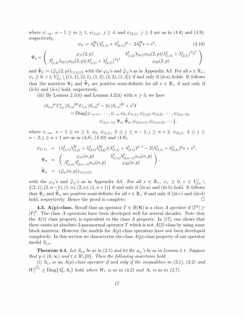
4.3. A(p)-class. Recall that an operator T ∈ B(H) is a class A operator if |T 2| ≥|T |2. The class A operators have been developed well for several decades. Note thatthe A(1) class property is equivalent to the class A property. In [17], one shows thatthere exists an absolute-2-paranormal operator T which is not A(2)-class by using someblock matrices. However the models for A(p)-class operators have not been developedcompletely. In this section we characterize the class A(p)-class property of our operatormodel St,n.

Theorem 4.4. Let St,n be as in (2.1) and let the aij’s be as in Lemma 2.1. Supposethat p ∈ (0,∞) and t ∈ R\0. Then the following assertions hold.

(i) St,1 is an A(p)-class operator if and only if the inequalities in (3.1), (3.2) and

W1p+1

1 ≥ Diagλ20, A1 hold, where W1 is as in (4.2) and A1 is as in (2.7).

17

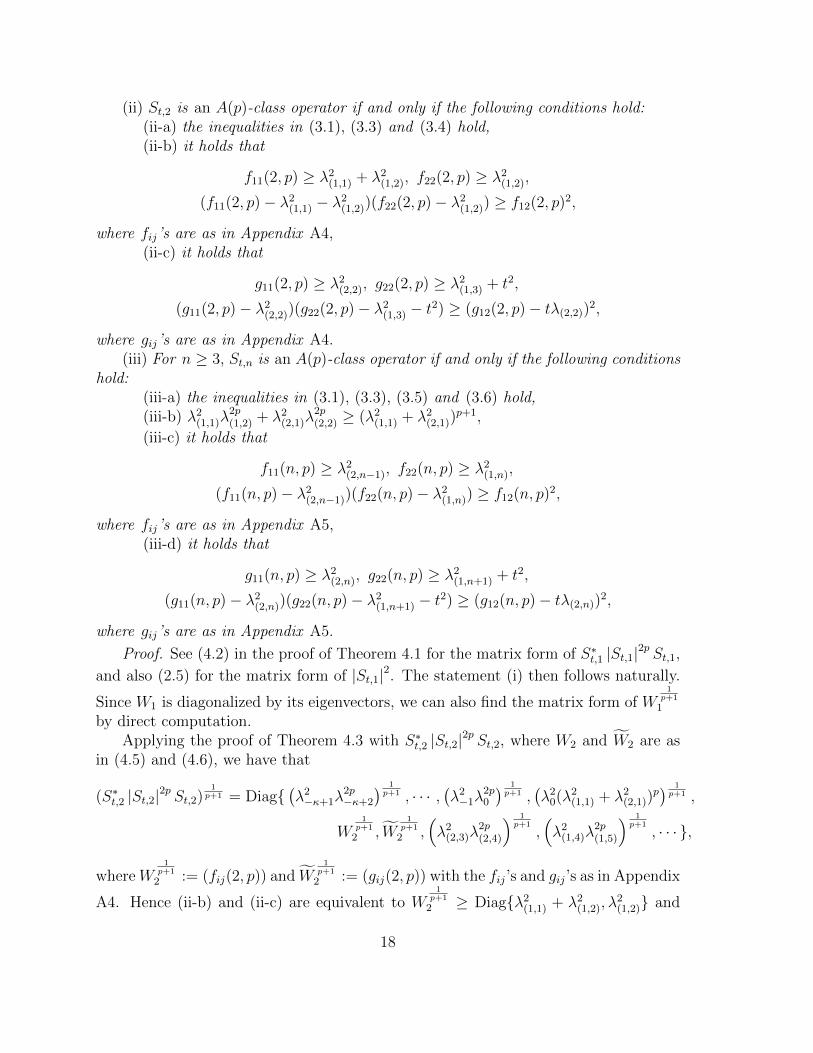
(ii) St,2 is an A(p)-class operator if and only if the following conditions hold:(ii-a) the inequalities in (3.1), (3.3) and (3.4) hold,(ii-b) it holds that

f11(2, p) ≥ λ2(1,1) + λ2(1,2), f22(2, p) ≥ λ2(1,2),

(f11(2, p)− λ2(1,1) − λ2(1,2))(f22(2, p)− λ2(1,2)) ≥ f12(2, p)2,

where fij’s are as in Appendix A4,(ii-c) it holds that

g11(2, p) ≥ λ2(2,2), g22(2, p) ≥ λ2(1,3) + t2,

(g11(2, p)− λ2(2,2))(g22(2, p)− λ2(1,3) − t2) ≥ (g12(2, p)− tλ(2,2))2,

where gij’s are as in Appendix A4.(iii) For n ≥ 3, St,n is an A(p)-class operator if and only if the following conditions

hold:(iii-a) the inequalities in (3.1), (3.3), (3.5) and (3.6) hold,(iii-b) λ2(1,1)λ

2p(1,2) + λ2(2,1)λ

2p(2,2) ≥ (λ2(1,1) + λ2(2,1))

p+1,

(iii-c) it holds that

f11(n, p) ≥ λ2(2,n−1), f22(n, p) ≥ λ2(1,n),

(f11(n, p)− λ2(2,n−1))(f22(n, p)− λ2(1,n)) ≥ f12(n, p)2,

where fij’s are as in Appendix A5,(iii-d) it holds that

g11(n, p) ≥ λ2(2,n), g22(n, p) ≥ λ2(1,n+1) + t2,

(g11(n, p)− λ2(2,n))(g22(n, p)− λ2(1,n+1) − t2) ≥ (g12(n, p)− tλ(2,n))2,

where gij’s are as in Appendix A5.

Proof. See (4.2) in the proof of Theorem 4.1 for the matrix form of S∗t,1 |St,1|2p St,1,

and also (2.5) for the matrix form of |St,1|2. The statement (i) then follows naturally.

Since W1 is diagonalized by its eigenvectors, we can also find the matrix form of W1p+1

1

by direct computation.Applying the proof of Theorem 4.3 with S∗t,2 |St,2|

2p St,2, where W2 and W2 are asin (4.5) and (4.6), we have that

(S∗t,2 |St,2|2p St,2)

1p+1 = Diag

(λ2−κ+1λ

2p−κ+2

) 1p+1 , · · · ,

(λ2−1λ

2p0

) 1p+1 ,

(λ20(λ

2(1,1) + λ2(2,1))

p) 1p+1 ,

W1p+1

2 , W1p+1

2 ,(λ2(2,3)λ

2p(2,4)

) 1p+1

,(λ2(1,4)λ

2p(1,5)

) 1p+1

, · · · ,

whereW1p+1

2 := (fij(2, p)) and W1p+1

2 := (gij(2, p)) with the fij’s and gij’s as in Appendix

A4. Hence (ii-b) and (ii-c) are equivalent to W1p+1

2 ≥ Diagλ2(1,1) + λ2(1,2), λ2(1,2) and

18

W1p+1

2 ≥ A2, respectively, where A2 is as in (2.8) with n = 2. And (ii-a) is obtainedeasily. For n ≥ 3, we obtain that(S∗t,n |St,n|

2p St,n) 1p+1

= Diag(λ2−κ+1λ

2p−κ+2

) 1p+1 , · · · ,

(λ2−1λ

2p0

) 1p+1 ,

(λ20(λ

2(1,1) + λ2(2,1))

p) 1p+1 ,(

λ2(1,1)λ2p(1,2) + λ2(2,1)λ

2p(2,2)

) 1p+1

,(λ2(1,2)λ

2p(1,3)

) 1p+1

, · · · ,(λ2(2,n−2)λ

2p(2,n−1)

) 1p+1

,(λ2(1,n−1)λ

2p(1,n)

) 1p+1

,W1p+1n , W

1p+1n ,

(λ2(2,n+1)λ

2p(2,n+2)

) 1p+1

, · · · ,

where

Wn =

(a11(n, p)λ

2(2,n−1) λ(1,n)λ(2,n−1)a12(n, p)

λ(1,n)λ(2,n−1)a12(n, p) a22(n, p)λ2(1,n)

)and

Wn =

(λ2(2,n)λ

2p(2,n+1) tλ(2,n)λ

2p(2,n+1)

tλ(2,n)λ2p(2,n+1) λ2(1,n+1)λ

2p(1,n+2) + t2λ2p(2,n+1)

).

By direct computations, we have that W1p+1n := (fij(n, p)) and W

1p+1n := (gij(n, p)) with

the fij and gij as in Appendix A5. Thus St,n is an A(p)-class operator if and only

if (iii-a) and (iii-b) hold, W1p+1n ≥ Diagλ2(2,n−1), λ2(1,n) and W

1p+1

2 ≥ An, where An is

as in (2.8). And (iii-c) and (iii-d) are equivalent to W1p+1n ≥ Diagλ2(2,n−1), λ2(1,n) and

W1p+1

2 ≥ An, respectively. Hence the proof is complete.

5. Examples

We consider some examples related to theorems in the previous sections.

Let Sλ be a weighted shift on the directed tree T2,κ with the λv below and considerSt,1 := Sλ + te(2,1) ⊗ e(1,1), with

λ(1,1) = λ(2,1) = 2, λm = 1, − κ+ 1 ≤ m ≤ 0,

λ(1,2) = 3, λ(1,k+2) = λ(2,k+1) = 4, k ∈ N.

p-Hyponormality. According to Theorem 3.2(i), we obtain that St,1 is p-hyponormal(0 < p <∞) if and only if ∆(p, t) ≥ 0, where

∆(p, t) :=

8 2t 0 02t t2 + 9 0 00 0 16 00 0 0 16

p

−

1 0 0 00 4 4 00 4 t2 + 4 3t0 0 3t 9

p

,

which is equivalent to the positivity of the 4× 4 matrix in Theorem 3.2 (i-b).

19

If we give a positive number p, we can estimate the range of t in R for thep-hyponormality of St,1. For example, a direct computation proves that St,1 is 2-hyponormal if and only if t ∈ [−δ, δ], where δ is the unique positive root of det ∆(2, t) =0. For some p > 0, it is not easy to find the range in t for the p-hyponormality of St,1,but we can find a subrange for the p-hyponormality of St,1. For example, taking p = 1

2

and t = 207100

, we have ∆(12, 207100

) ≥ 0, i.e., S 207100

,1 is 12-hyponormal.

Absolute-p-paranormality. We compute W1 appearing in (4.2) using insteadpart of the result from the computation of ∆(p, t) above and direct computationfrom S∗t,1(S

∗t,1St,1)

pSt,1. According to Theorem 4.1(i), we recall that St,1 is absolute-p-paranormal (0 < p <∞) if and only if Ω1(p, t, s) ≥ 0 for all s > 0, where

Ω1(p, t, s) =

1 0 0 00 2 2 00 0 t 3

8 2t 0 02t t2 + 9 0 00 0 16 00 0 0 16

p

1 0 00 2 00 2 t0 0 3

−(p+ 1)sp

1 0 00 8 2t0 2t t2 + 9

+ psp+1I

as in (4.1). By some computations, we have that S 5325,1[S 21

10,1, or S 209

100,1, resp.] is absolute-

2-paranormal[absolute-1-paranormal, or absolute-12-paranormal, resp.].

p-Paranormality. In what follows, we use for convenience of computation analternative form of the relevant matrix obtained using the polar decomposition of St,1.According to Theorem 4.3(i), we obtain that St,1 is p-paranormal (0 < p < ∞) if andonly if Ψ1(p, t, s) ≥ 0 for all s > 0, where

Ψ1(p, t, s) =

1 0 00 8 2t0 2t t2 + 9

p/2

U∗

8 2t 0 02t t2 + 9 0 00 0 16 00 0 0 16

p

U

1 0 00 8 2t0 2t t2 + 9

p/2

−2s

1 0 00 8 2t0 2t t2 + 9

p

+ s2I

with

U =

1 0 00 u11(1) u12(1)0 u21(1) u22(1)0 u31(1) u32(1)

=

1 0 00 2 00 2 t0 0 3

1 0 0

0 8 2t0 2t t2 + 9

−1/2 ,where uij(1) are as in Lemma 4.2(i). By some computations, we have that S 11

5,1[S 21

10,1,

or S 5225,1, resp.] is 2-paranormal[1-paranormal, or 1

2-paranormal, resp.].

20

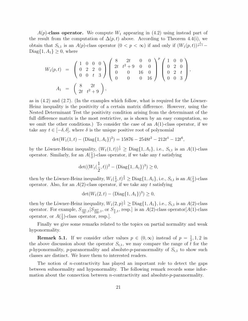
A(p)-class operator. We compute W1 appearing in (4.2) using instead part ofthe result from the computation of ∆(p, t) above. According to Theorem 4.4(i), we

obtain that St,1 is an A(p)-class operator (0 < p < ∞) if and only if (W1(p, t))1p+1−

Diag1, A1 ≥ 0, where

W1(p, t) =

1 0 0 00 2 2 00 0 t 3

8 2t 0 02t t2 + 9 0 00 0 16 00 0 0 16

p

1 0 00 2 00 2 t0 0 3

,

A1 =

(8 2t2t t2 + 9

),

as in (4.2) and (2.7). (In the examples which follow, what is required for the Lowner-Heinz inequality is the positivity of a certain matrix difference. However, using theNested Determinant Test the positivity condition arising from the determinant of thefull difference matrix is the most restrictive, as is shown by an easy computation, sowe omit the other conditions.) To consider the case of an A(1)-class operator, if wetake any t ∈ [−δ, δ], where δ is the unique positive root of polynomial

det(W1(1, t)− (Diag1, A1)2) = 15876− 2548t2 − 212t4 − 12t6,

by the Lowner-Heinz inequality, (W1(1, t))12 ≥ Diag1, A1, i.e., St,1 is an A(1)-class

operator. Similarly, for an A(12)-class operator, if we take any t satisfying

det((W1(1

2, t))2 − (Diag1, A1)3) ≥ 0,

then by the Lowner-Heinz inequality, W1(12, t)

23 ≥ Diag1, A1, i.e., St,1 is an A(1

2)-class

operator. Also, for an A(2)-class operator, if we take any t satisfying

det(W1(2, t)− (Diag1, A1)3) ≥ 0,

then by the Lowner-Heinz inequality, W1(2, p)13 ≥ Diag1, A1, i.e., St,1 is an A(2)-class

operator. For example, S 10350,1[S 207

100,1, or S 9

5,1, resp.] is an A(2)-class operator[A(1)-class

operator, or A(12)-class operator, resp.].

Finally we give some remarks related to the topics on partial normality and weakhyponormality.

Remark 5.1. If we consider other values p ∈ (0,∞) instead of p = 12, 1, 2 in

the above discussion about the operator St,1, we may compare the range of t for thep-hyponormality, p-paranormality and absolute-p-paranormality of St,1 to show suchclasses are distinct. We leave them to interested readers.

The notion of n-contractivity has played an important role to detect the gapsbetween subnormality and hyponormality. The following remark records some infor-mation about the connection between n-contractivity and absolute-p-paranormality.

21

Remark 5.2. Recall that T ∈ B(H) is 2-contractive if T ∗2T 2 − 2T ∗T + I ≥ 0([1]). Clearly, if T is absolute-1-paranormal then it is 2-contractive. Our model St,1can show these properties are distinct. For example, S 11

5,1 is 2-contractive but not

absolute-1-paranormal because the matrix Ω1 is not positive when s = 15.

The following example related to our operator model is interesting in its own right.

Remark 5.3. If we allow t = 0 in the model, we may create some examples of2-isometries which we believe to be new. Recall that T ∈ B(H) is a 2-isometry ifI − 2T ∗T + T ∗2T 2 = 0, that every isometry is a 2-isometry (including the unilateralshift), and that the standard non-isometric 2-isometry is the Dirichlet shift WD, withweights

√2,√

3/2,√

4/3,√

5/4, . . .. Observe that the WD is a strict expansion, in thesense that ‖WDx‖ > ‖x‖ for all x 6= 0 (any 2-isometry is at least a weak expansion).If we use (for example) κ = 4 with

λ−3 =√

2, λ−2 =√

3/2, λ−1 =√

4/3, λ0 =√

5/4,

λ2,n = 1 (n ≥ 1), λ1,1 =√

1/5, λ1,n =√n/(n− 1) (n ≥ 2),

we produce a 2-isometry which is neither an isometry, strictly expansive, nor a trivialdirect sum of the Dirichlet shift with an isometry.

Appendix - expressions of polynomials

We give the exact expressions of polynomials which appeared in the previous sec-tions.A1. Polynomials in Theorem 3.2:

b11(1, p) = λ2(1,1)((β1 − λ2

(1,1) − λ2(2,1))α

p1β1 + (λ2

(1,1) + λ2(2,1) − α1)β

p1α1)/(γ1δ

2),

b12(1, p) = λ(1,1)λ(2,1)((λ2(1,2) − α1)α

p1β1 + (β1 − λ2

(1,2))α1βp1 )/(γ1δ

2),

b13(1, p) = tλ(1,1)λ(1,2)λ(2,1)(α1βp1 − α

p1β1)/(γ1δ

2),

b22(1, p) = ((λ2(1,2) − α1)(λ

2(1,2)λ

2(2,1) + λ2

(1,1)(α1 − λ2(1,1) − λ2

(2,1)))αp1 + (β1 − λ2

(1,2))(λ2(1,2)λ

2(2,1) + λ2

(1,1)(β1 − λ2(1,1)

−λ2(2,1)))β

p1 )/(γ1δ

2),

b23(1, p) = tλ(1,2)((λ2(1,1)(λ

2(1,1) + λ2

(2,1) − α1) − λ2(1,2)λ

2(2,1))α

p1 + (λ2

(1,1)(β1 − λ2(1,1) − λ2

(2,1)) + λ2(1,2)λ

2(2,1))β

p1 )/(γ1δ

2),

b33(1, p) = λ2(1,2)(((β1−λ

2(1,2))λ

2(2,1)+λ

2(1,1)(λ

2(1,1)+λ

2(2,1)−α1))α

p1+((λ2

(1,2)−α1)λ2(2,1)+λ

2(1,1)(β1−λ

2(1,1)−λ

2(2,1)))β

p1 )/(γ1δ

2),

b11(n, p) = ((λ2(1,n+1) − αn)αp

n + (βn − λ2(1,n+1))β

pn)/γn; b12(n, p) = tλ(1,n+1)(β

pn − αp

n)/γn,

b22(n, p) = ((βn − λ2(1,n+1))α

pn + (λ2

(1,n+1) − αn)βpn)/γn,

where δ = (λ2(1,2)λ

2(2,1) + λ2

(1,1)(t2 + λ2

(1,2)))1/2.

A2. Polynomials in Theorem 4.1:

ω11(1, p) = a11(1, p)λ20 − (p + 1)λ2

0sp + psp+1; ω22(1, p) = a22(1, p)λ

2(1,1) + λ2

(2,1)λ2p(2,2)

− (p + 1)(λ2(1,1) + λ2

(2,1))sp + psp+1,

ω33(1, p) = t2λ2p(2,2)

+ λ2(1,2)λ

2p(1,3)

− (p + 1)(t2 + λ2(1,2))s

p + psp+1,

ω11(2, p) = λ2(1,1)λ

2p(1,2)

+ a11(2, p)λ2(2,1) − (1 + p)sp(λ2

(1,1) + λ2(2,1)) + ps1+p,

ω11(n, p) = a11(n, p)λ2(2,n−1) − (1 + p)spλ2

(2,n−1) + ps1+p; ω22(n, p) = a22(n, p)λ2(1,n) − (1 + p)spλ2

(1,n) + ps1+p,

ω11(n, p) = λ2(2,n)λ

2p(2,n+1)

−(1+p)spλ2(2,n)+ps

1+p; ω22(n, p) = λ2(1,n+1)λ

2p(1,n+2)

+t2λ2p(2,n+1)

−(1+p)sp(t2+λ2(1,n+1))+ps

1+p.

A3. Polynomials in Theorem 4.3:

ϕ11(1, p) = λ2p0 a11(1, p) − 2sλ

2p0 + s2; ϕ12(1, p) = λ

p0a12(1, p)φ1(1); ϕ13(1, p) = λ

p0a12(1, p)φ2(1),

ϕ22(1, p) = a22(1, p)φ1(1)2 + λ

2p(1,3)

φ3(1)2 + λ

2p(2,2)

φ4(1)2 − 2sa11(1, p) + s2,

ϕ23(1, p) = a22(1, p)φ1(1)φ2(1) + λ2p(1,3)

φ3(1)φ5(1) + λ2p(2,2)

φ4(1)φ6(1) − 2sa12(1, p),

ϕ33(1, p) = a22(1, p)φ2(1)2 + λ

2p(1,3)

φ5(1)2 + λ

2p(2,2)

φ6(1)2 − 2sa22(1, p) + s2,

ϕ11(2, p) = (λ2(1,1)λ

2p(1,2)

+ a11(2, p)λ2(2,1))(λ

2(1,1) + λ2

(2,1))p−1 − 2s(λ2

(1,1) + λ2(2,1))

p + s2,

ϕ11(n, p) = a11(n, p)λ2p(2,n−1)

− 2sλ2p(2,n−1)

+ s2; ϕ22(n, p) = a22(n, p)λ2p(1,n)

− 2sλ2p(1,n)

+ s2,

ϕ11(n, p) = λ2p(2,n+1)

φ1(n)2 + λ

2p(1,n+2)

φ4(n)2 − 2sa11(n, p) + s2,

22

ϕ12(n, p) = λ2p(1,n+2)

φ4(n)φ6(n) + λ2p(2,n+1)

φ1(n)φ2(n) − 2sa12(n, p),

ϕ22(n, p) = λ2p(2,n+1)

φ2(n)2 + λ

2p(1,n+2)

φ6(n)2 − 2sa22(n, p) + s2,

whereφ1(n) = a11(n,

p2)u11(n)+a12(n,

p2)u12(n); φ2(n) = a12(n,

p2)u11(n)+a22(n,

p2)u12(n); φ3(n) = a11(n,

p2)u31(n)+a12(n,

p2)u32(n),

φ4(n) = a11(n,p2)u21(n)+a12(n,

p2)u22(n); φ5(n) = a12(n,

p2)u31(n)+a22(n,

p2)u32(n); φ6(n) = a12(n,

p2)u21(n)+a22(n,

p2)u22(n).

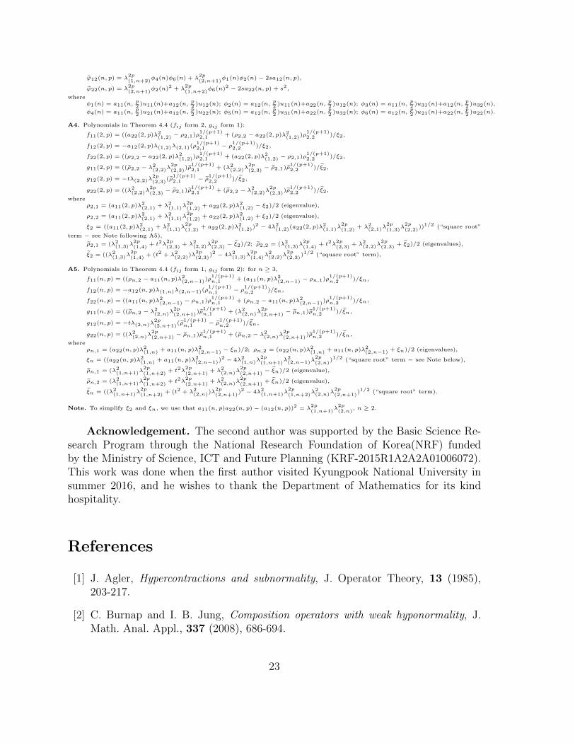
A4. Polynomials in Theorem 4.4 (fij form 2, gij form 1):

f11(2, p) = ((a22(2, p)λ2(1,2) − ρ2,1)ρ

1/(p+1)2,1 + (ρ2,2 − a22(2, p)λ

2(1,2))ρ

1/(p+1)2,2 )/ξ2,

f12(2, p) = −a12(2, p)λ(1,2)λ(2,1)(ρ1/(p+1)2,1 − ρ

1/(p+1)2,2 )/ξ2,

f22(2, p) = ((ρ2,2 − a22(2, p)λ2(1,2))ρ

1/(p+1)2,1 + (a22(2, p)λ

2(1,2) − ρ2,1)ρ

1/(p+1)2,2 )/ξ2,

g11(2, p) = ((ρ2,2 − λ2(2,2)λ

2p(2,3)

)ρ1/(p+1)2,1 + (λ2

(2,2)λ2p(2,3)

− ρ2,1)ρ1/(p+1)2,2 )/ξ2,

g12(2, p) = −tλ(2,2)λ2p(2,3)

(ρ1/(p+1)2,1 − ρ

1/(p+1)2,2 )/ξ2,

g22(2, p) = ((λ2(2,2)λ

2p(2,3)

− ρ2,1)ρ1/(p+1)2,1 + (ρ2,2 − λ2

(2,2)λ2p(2,3)

)ρ1/(p+1)2,2 )/ξ2,

whereρ2,1 = (a11(2, p)λ

2(2,1) + λ2

(1,1)λ2p(1,2)

+ a22(2, p)λ2(1,2) − ξ2)/2 (eigenvalue),

ρ2,2 = (a11(2, p)λ2(2,1) + λ2

(1,1)λ2p(1,2)

+ a22(2, p)λ2(1,2) + ξ2)/2 (eigenvalue),

ξ2 = ((a11(2, p)λ2(2,1) + λ2

(1,1)λ2p(1,2)

+ a22(2, p)λ2(1,2))

2 − 4λ2(1,2)(a22(2, p)λ

2(1,1)λ

2p(1,2)

+ λ2(2,1)λ

2p(1,3)

λ2p(2,2)

))1/2 (“square root”

term − see Note following A5),

ρ2,1 = (λ2(1,3)λ

2p(1,4)

+ t2λ2p(2,3)

+ λ2(2,2)λ

2p(2,3)

− ξ2)/2; ρ2,2 = (λ2(1,3)λ

2p(1,4)

+ t2λ2p(2,3)

+ λ2(2,2)λ

2p(2,3)

+ ξ2)/2 (eigenvalues),

ξ2 = ((λ2(1,3)λ

2p(1,4)

+ (t2 + λ2(2,2))λ

2p(2,3)

)2 − 4λ2(1,3)λ

2p(1,4)

λ2(2,2)λ

2p(2,3)

)1/2 (“square root” term),

A5. Polynomials in Theorem 4.4 (fij form 1, gij form 2): for n ≥ 3,

f11(n, p) = ((ρn,2 − a11(n, p)λ2(2,n−1))ρ

1/(p+1)n,1 + (a11(n, p)λ

2(2,n−1) − ρn,1)ρ

1/(p+1)n,2 )/ξn,

f12(n, p) = −a12(n, p)λ(1,n)λ(2,n−1)(ρ1/(p+1)n,1 − ρ

1/(p+1)n,2 )/ξn,

f22(n, p) = ((a11(n, p)λ2(2,n−1) − ρn,1)ρ

1/(p+1)n,1 + (ρn,2 − a11(n, p)λ

2(2,n−1))ρ

1/(p+1)n,2 )/ξn,

g11(n, p) = ((ρn,2 − λ2(2,n)λ

2p(2,n+1)

)ρ1/(p+1)n,1 + (λ2

(2,n)λ2p(2,n+1)

− ρn,1)ρ1/(p+1)n,2 )/ξn,

g12(n, p) = −tλ(2,n)λ2p(2,n+1)

(ρ1/(p+1)n,1 − ρ

1/(p+1)n,2 )/ξn,

g22(n, p) = ((λ2(2,n)λ

2p(2,n+1)

− ρn,1)ρ1/(p+1)n,1 + (ρn,2 − λ2

(2,n)λ2p(2,n+1)

)ρ1/(p+1)n,2 )/ξn,

whereρn,1 = (a22(n, p)λ

2(1,n) + a11(n, p)λ

2(2,n−1) − ξn)/2; ρn,2 = (a22(n, p)λ

2(1,n) + a11(n, p)λ

2(2,n−1) + ξn)/2 (eigenvalues),

ξn = ((a22(n, p)λ2(1,n) + a11(n, p)λ

2(2,n−1))

2 − 4λ2(1,n)λ

2p(1,n+1)

λ2(2,n−1)λ

2p(2,n)

)1/2 (“square root” term − see Note below),

ρn,1 = (λ2(1,n+1)λ

2p(1,n+2)

+ t2λ2p(2,n+1)

+ λ2(2,n)λ

2p(2,n+1)

− ξn)/2 (eigenvalue),

ρn,2 = (λ2(1,n+1)λ

2p(1,n+2)

+ t2λ2p(2,n+1)

+ λ2(2,n)λ

2p(2,n+1)

+ ξn)/2 (eigenvalue),

ξn = ((λ2(1,n+1)λ

2p(1,n+2)

+ (t2 + λ2(2,n))λ

2p(2,n+1)

)2 − 4λ2(1,n+1)λ

2p(1,n+2)

λ2(2,n)λ

2p(2,n+1)

)1/2 (“square root” term).

Note. To simplify ξ2 and ξn, we use that a11(n, p)a22(n, p) − (a12(n, p))2 = λ

2p(1,n+1)

λ2p(2,n)

, n ≥ 2.

Acknowledgement. The second author was supported by the Basic Science Re-search Program through the National Research Foundation of Korea(NRF) fundedby the Ministry of Science, ICT and Future Planning (KRF-2015R1A2A2A01006072).This work was done when the first author visited Kyungpook National University insummer 2016, and he wishes to thank the Department of Mathematics for its kindhospitality.

References

[1] J. Agler, Hypercontractions and subnormality, J. Operator Theory, 13 (1985),203-217.

[2] C. Burnap and I. B. Jung, Composition operators with weak hyponormality, J.Math. Anal. Appl., 337 (2008), 686-694.

23

[3] C. Burnap, I. B. Jung and A. Lambert, Separating partial normality classes withcomposition operators, J. Operator Theory, 53 (2005), 381-397.

[4] R. Curto and L. Fialkow, Recursively generated weighted shifts and the subnormalcompletion problem, Integr. Equ. Oper. Theory, 17 (1993), 202-246.

[5] W. Donoghue, On the perturbation of spectra, Comm. Pure Appl. Math., 18(1965), 559–579.

[6] G. Exner, I. B. Jung and M. R. Lee, Block matrix operators and weak hyponor-malities, Integr. Equ. Oper. Theory, 65 (2009), 345-362.

[7] G. Exner, I. B. Jung, E. Y. Lee and M. R. Lee, Partially normal compositionoperators relevant to weighted directed trees , J. Math. Anal. Appl., 450 (2017),444-460.

[8] G. Exner, I. B. Jung, E. Y. Lee and M. R. Lee, Gaps of operators via rank-oneperturbations, J. Math. Anal. Appl., 376 (2011), 576-587.

[9] G. Exner, I. B. Jung, E. Y. Lee and M. Seo, On weighted adjacency operatorsassociated to directed graphs, Filomat, 31 (2017), 4085-4104.

[10] C. Foias, I. B. Jung, E. Ko and C. Pearcy, On rank-one perturbations of normaloperators, J. Funct. Anal., 253 (2007), 628-646.

[11] C. Foias, I. B. Jung, E. Ko and C. Pearcy, Rank-one perturbations of normaloperators. II, Indiana Univ. Math. J., 57 (2008), 2745-2760.

[12] J. Fujii, M. Fujii, H. Sasaoka, Y. Watatani, The spectrum of an infinite directedgraph, Math. Japon., 36 (1991), 607-625.

[13] M. Fujii, T. Sano, H. Sasaoka, The index of an infinite directed graph, Math.Japon., 35 (1990), 561-567.

[14] M. Fujii, H. Sasaoka, Y. Watatani, Adjacency operators of infinite directed graphs,Math. Japon., 34 (1989), 727-735.

[15] M. Fujii, H. Sasaoka, Y. Watatani, The numerical radius of an infinite directedgraph, Math. Japon., 35 (1990), 577-582.

[16] T. Furuta, Invitation to linear operators, Taylor & Francis, Ltd., London, 2001.

[17] T. Furuta, M. Ito and T. Yamazaki, A subclass of paranormal operators includingclass of log-hyponormal and several related classes, Sci. Math., 1 (1998), 389-403.

[18] M. Ito and T. Yamazaki, Relations between two inequalities (Br/2Ap Br/2)r/(p+r) ≥Br and Ap ≥ (Ap/2BrAp/2)p/(p+r) and their applications, Integr. Equ. Oper. The-ory, 44 (2002), 442-450.

24

[19] Z. Jab lonski, I. B. Jung and J. Stochel, Weighted shifts on directed trees, Mem.Amer. Math. Soc., 216 (2012), no. 1017, viii+ 106 pp.

[20] Z. Jab lonski, I. B. Jung and J. Stochel, A non-hyponormal operator generatingStieltjes moment sequences, J. Funct. Anal., 262 (2012), 3946-3980.

[21] S. Jitomirskaya and B. Simon, Operators with singular continuous spectrum. III.Almost periodic Schrodinger operators, Comm. Math. Phys., 165 (1994), 201-205.

[22] I. B. Jung, M. R. Lee and P. S. Lim, Gaps of operators. II, Glasg. Math. J., 47(2005), 461-469.

[23] I. B. Jung, P. S. Lim and S. S. Park, Gaps of operators, J. Math. Anal. Appl.,304 (2005), 87-95.

[24] R. Del Rio, N. Makarov and B. Simon, Operators with singular continuous spec-trum. II. Rank one operators, Comm. Math. Phys., 165 (1994), 59-67.

[25] Wolfram Research, Inc. Mathematica, Version 10.0, Wolfram Research, Inc. Cham-paign, IL, 1996.

[26] D. Xia, Spectral Theory of Hyponormal Operators, Birkhauser Verlag, Basel, 1983.

[27] T. Yamazaki and M. Yanagida, A further generalization of paranormal operators,Sci. Math., 3 (2000), 23-31.

G. ExnerBucknell University, Lewisburg, Pennsylvania 17837, USAE-mail: exner@bucknell.edu

I. B. Jung, E. Y. Lee and M. SeoKyungpook National University, Daegu 41566, KoreaE-mail: ibjung@knu.ac.kr (I. B. Jung), eunyounglee@knu.ac.kr (E. Y. Lee), mjseo@knu.ac.kr(M. Seo)

25