The University of AkronIdeaExchange@UAkron

Honors Research Projects The Dr. Gary B. and Pamela S. Williams HonorsCollege

Spring 2018

Reaction Kinetics of the Hydrogenation of Phenolin a Tubular ReactorMichael Selzermss118@zips.uakron.edu

Please take a moment to share how this work helps you through this survey. Your feedback will beimportant as we plan further development of our repository.Follow this and additional works at: http://ideaexchange.uakron.edu/honors_research_projects

Part of the Catalysis and Reaction Engineering Commons

This Honors Research Project is brought to you for free and open access by The Dr. Gary B. and Pamela S. WilliamsHonors College at IdeaExchange@UAkron, the institutional repository of The University of Akron in Akron, Ohio,USA. It has been accepted for inclusion in Honors Research Projects by an authorized administrator ofIdeaExchange@UAkron. For more information, please contact mjon@uakron.edu, uapress@uakron.edu.

Recommended CitationSelzer, Michael, "Reaction Kinetics of the Hydrogenation of Phenol in a Tubular Reactor" (2018). Honors ResearchProjects. 643.http://ideaexchange.uakron.edu/honors_research_projects/643

Reaction Kinetics of the Hydrogenation of Phenol in a Tubular Reactor

Advisor

Dr. George Chase

By

Michael Selzer

4/27/2018

1

Table of Contents

Executive Summary ........................................................................................................................ 2

Introduction ..................................................................................................................................... 4

Background ..................................................................................................................................... 4

Modeling ......................................................................................................................................... 5

Genetic Algorithm Optimization .................................................................................................. 11

Experimental Methods .................................................................................................................. 12

Results ........................................................................................................................................... 13

One-Dimensional Modeling ...................................................................................................... 13

Test of the genetic algorithm ..................................................................................................... 16

Discussion ..................................................................................................................................... 17

Conclusions ................................................................................................................................... 18

Nomenclature ................................................................................................................................ 19

References ..................................................................................................................................... 20

Appendix A: One-dimensional model spreadsheet ....................................................................... 21

Appendix B : Source for the genetic algorithm test program ....................................................... 22

Appendix C: Source for the genetic curve fitting program........................................................... 29

2

Executive Summary

Cyclohexanone is a product used in the production of polyamides. It is commonly produced by

the partial hydrogenation of phenol over a palladium catalyst. This route to cyclohexanone can

continue to form cyclohexanol, which must be separated. The amount of cyclohexanol that is

produced can be reduced by increasing the selectivity to cyclohexanone. To increase the

selectivity towards cyclohexanone, a new reactor design has been proposed. The proposed

reactor design is a tubular reactor with a hydrophobic, electrospun PVDF membrane as the

catalyst support and the means to separate the hydrogen and aqueous phenol. The characteristics

of the hydrogenation reaction are assessed by creating models for the system and calculating the

pre-exponential factor, activation energy, and the rate law for the reaction.

The reactor was run using tubes with diameters of 0.187 in and 0.25 in and catalyst loadings of

40, 50, and 60 g/m2 at constant flow rates of hydrogen and solution for 10 hours. The

concentration over time was determined by sampling on two hour intervals and measuring

concentration with a gas chromatograph. One-dimensional and two-dimensional models for the

concentration profile in the reactor are derived from the general mass balance and species

balance equations. A model for the reactor considering a one-dimensional variation in

concentration has been derived and fitted to the data with a non-linear least squares regression.

Based on this model the pre-exponential factor was 2.50 x 104, the activation energy was 76.9

kJ/mol and the reaction order with respect to phenol was 0.171. The one-dimensional model

may not be the best approach since it does not account for diffusion in the radial direction. A

two-dimensional model has been derived from transport equations. The model equations will be

fitted to a large set of data using a genetic algorithm. The genetic algorithm has been

programmed in C. Testing of the genetic algorithm with an elliptic paraboloid has found that the

genetic algorithm is effective, reaching a convergence of 10-6

within 800000 generations with

three significant digits of accuracy.

The development of a model and program for fitting data is beneficial to those continuing to

assess the performance of the reactor design. The author’s ability to model a physical system

using concepts from transport phenomena has been reinforced. The author has also expanded his

knowledge of programming in C to include file input and output, dynamic array allocation, and

bitwise operations. For future work, additional data should be collected and analyzed using the

3

genetic algorithm curve fitting program. When the reactor performance with a single tube is

characterized, tests should be done with a number of tubes to find how performance improves

under this condition.

4

Introduction

Cyclohexanone is commonly produced through the partial hydrogenation of phenol over a

palladium catalyst [1]. This route is preferred since it is exothermic, but has the possibility of

continuing to form cyclohexanol, which must be separated [1]. Authors have explored the use of

several supported catalysts to increase the selectivity to cyclohexanone [2,3,4]. The

effectiveness of this method can be improved by using a reactor design that improves the

selectivity towards cyclohexanone. A tubular reactor design where the catalyst is supported on a

tube of electrospun poly (vinylidene fluoride) (PVDF) is proposed to achieve improved

selectivity. The reaction rate law, activation energy, and pre-exponential factor are key to

understanding how to improve the performance of such a reactor.

Background

PVDF is a hydrophobic material, due to the electronegative fluorine atoms in its repeating unit.

The hydrophobic fibers repel the aqueous phenol solution, limiting the diffusion of phenol to the

surface where it can react. A similar reactor design has been analyzed by Itoh and Xu [5]. Their

design focused on the gas phase hydrogenation of phenol over palladium based membranes [5].

There is published data for the kinetics of the phenol hydrogenation reaction in the gas phase.

Itoh and Xu found that the activation energy ranged from 12.48 to 15.28 kJ/mol for the gas-phase

reaction [5]. The liquid phase reaction has been shown to occur at low temperatures (30°C), but

requires long reaction times to reach a high conversion [4]. Other researchers have proposed

power law models for the rate law [1,2]. Mahata and Vishwanathan found that the order with

respect to phenol can vary between -0.13 and 0.65 in the gas phase depending on the temperature

and the type of catalyst used [2]. They also report that the order with respect to hydrogen varied

between 0.39 and 0.98 [2]. Neri, et al. found that a varied between -1 and 1 and that b varied

between 1 and 2 [1].

A model that can be used to determine the kinetic parameters can be found using transport

equations. The system of equations that are found from the reactor model can be solved

numerically using successive substitution and improved Euler methods. Since these equations

can only be solved numerically, a genetic algorithm is a simple method to fit the experimental

data to the model. A genetic algorithm is an optimization method that involves choosing the

5

next set of possible solutions by modifying the members of the current set that best fit the model

[6]. Genetic optimization does not require that the derivative of the objective function be

available, and can have operations added that ensure that the global minimum of the objective

function is found [6]. The technique has been used to fit reaction kinetic data before [7].

Modeling

Figure 1 shows a PFD of the experimental setup

Figure 1: PFD of the experimental setup.

Figure 2 shows the geometry of the reactor.

6

Figure 2: Details of the reactor geometry. The drawing on the left shows a view of the cross-

sectional area of the reactor and the drawing on the right shows a side view of the reactor.

If a mole balance around the vial in the experimental setup is written,

𝑑𝑁

𝑑𝑡= 𝑛𝑖𝑛 − 𝑛𝑜𝑢𝑡 (1)

The moles of phenol in the vial will decrease over time as it is consumed by the reaction. If the

vial is considered well-mixed, the concentration of phenol in the stream exiting the vial will be

equal to the concentration of phenol in the vial and the above equation may be rewritten as

𝑑𝑛𝑜𝑢𝑡

𝑑𝑡= 𝑛𝑖𝑛 − 𝑛𝑜𝑢𝑡 (2)

Since the reactor is a recirculating tubular reaction, the moles of phenol entering the vial will

decrease over time. The above equation can be further simplified if the volume of solution in the

vial is considered to be constant. The volumetric flow rate into the reactor is equal to the flow

rate out of the vial and it is known that the flow rate is also constant.

𝑉𝑣𝑖𝑎𝑙𝑑𝐶𝑝,𝑜𝑢𝑡

𝑑𝑡= 𝑣(𝐶𝑝,𝑖𝑛 − 𝐶𝑝,𝑜𝑢𝑡) (3)

Next, a mole balance around the reactor can be written using the general form for a PFR [8].

𝑑𝑛

𝑑𝑉= 𝑅𝐴 (4)

The cross-sectional area can be factored out since the concentration in a PFR varies only in the z

direction [5].

𝑑𝑛

𝐴𝑐𝑑𝑧= 𝑅𝐴 (5)

7

As in the mole balance for the vial, the volumetric flow rate is constant so the equation can be

rewritten in terms of concentration.

𝑣𝑑𝐶

𝐴𝑐𝑑𝑧= 𝑅𝐴 (6)

The right hand side of the equation is rewritten based on a power law equation for the reaction

rate.

𝑣𝑑𝐶

𝐴𝑐𝑑𝑧= 𝑘𝑎𝑐𝑎𝑡𝐶

𝑎𝑃𝑏 (7)

Equations 3 and 7 can be solved numerically to obtain the solution for a model of the reactor in

one dimension. Each of these equations can be solved using a modified Euler’s method [9]. The

equation needs to be rewritten in the form

𝑑𝑋

𝑑𝑡= 𝑓(𝑋, 𝑡) (8)

Then the final value is found by equations 9 and 10

𝑋𝑖𝑝 = 𝑋𝑖 + ℎ𝑓(𝑋𝑖, 𝑡𝑖) (9)

𝑋𝑖+1 = 𝑋𝑖 +1

2ℎ (𝑓(𝑋𝑖, 𝑡𝑖) + 𝑓(𝑋𝑖𝑝, 𝑡𝑖+1)) (10)

Where h is the step size. Equations 9 and 10 are evaluated in a loop until t is equal to the final

value of the differential equation. The calculated values can be fitted using a nonlinear least

squares method.

This model for the reaction has its limitations in effectively describing the reaction because it

suggests that the reaction occurs in the bulk, while it is known that the reaction can only occur at

the active sites of the catalyst. For this reason, it should not be assumed that the solution is well

mixed in the r direction. The flow regime in the system is also laminar, and will not be mixed

well.

The reaction requires the transport of two species to catalyst active sites in order for the reaction

to occur. Hydrogen is flowing inside the PVDF tube and will not experience any sort of

8

limitations in mass transfer. This assumption can be made since hydrogen is a gas and will

therefore have a high rate of diffusion. The general species balance equation is

𝜕𝐶𝐴

𝜕𝑡+ ∇ ∙ 𝑁𝐴 = 𝑅𝐴 (11)

Since the reactor operates at steady state and without a bulk reaction.

∇ ∙ 𝑁𝐴 = 0 (12)

By expanding the divergence in cylindrical coordinates [10]

1

𝑟

𝜕(𝑟𝑁𝐴)

𝜕𝑟+

1

𝑟

𝜕𝑁𝐴

𝜕𝜃+

𝜕𝑁𝐴

𝜕𝑧= 0 (13)

The molar flux does not vary in the angular direction.

1

𝑟

𝜕(𝑟𝑁𝐴)

𝜕𝑟+

𝜕𝑁𝐴

𝜕𝑧= 0 (14)

The molar flux can be rewritten as the sum of the diffusion and convection in each direction.

1

𝑟

𝜕

𝜕𝑟(𝑟𝐶𝐴𝑣𝑟 + 𝑟𝐽𝐴𝑟) +

𝜕

𝜕𝑧(𝐶𝐴𝑧𝑣𝑧 + 𝐽𝐴𝑧) = 0 (15)

Diffusion can be neglected in the z direction since there is forced convection in this direction.

Convection can be neglected in the r direction since the fluid flow is primarily in the z direction.

1

𝑟

𝜕

𝜕𝑟𝑟𝐽𝐴𝑟 +

𝜕

𝜕𝑧(𝐶𝐴𝑣𝑧) = 0 (16)

By integrating over the cross sectional area,

∫ ∫1

𝑟

𝑑

𝑑𝑟(𝑟𝐽𝐴𝑟)𝑟𝑑𝑟𝑑𝜃

𝑅1

𝑅0

2𝜋

0+ ∫ ∫

𝑑

𝑑𝑧(𝐶𝐴𝑣𝑧)𝑟𝑑𝑟𝑑𝜃

𝑅1

𝑅0

2𝜋

0= 0 (17)

2𝜋 ∫𝑑

𝑑𝑟(𝑟𝐽𝐴𝑟)𝑑𝑟

𝑅1

𝑅0+ 2𝜋 ∫

𝑑

𝑑𝑧(𝐶𝐴𝑣𝑧)𝑟𝑑𝑟

𝑅1

𝑅0= 0 (18)

2𝜋(𝑅1𝐽𝐴𝑟(𝑅1) − 𝑅0𝐽𝐴𝑟(𝑅0)) + 2𝜋 ∫𝑑

𝑑𝑧(𝐶𝐴𝑣𝑧)𝑟𝑑𝑟

𝑅1

𝑅0= 0 (19)

The bulk average quantities can be used to solve the second integral.

2𝜋(𝑅1𝐽𝐴𝑟(𝑅1) − 𝑅0𝐽𝐴𝑟(𝑅0)) + 2𝜋 ∫𝑑

𝑑𝑧(𝐶𝐴𝑏⟨𝑣𝑧⟩)𝑟𝑑𝑟

𝑅1

𝑅0= 0 (20)

9

2𝜋(𝑅1𝐽𝐴𝑟(𝑅1) − 𝑅0𝐽𝐴𝑟(𝑅0)) +2𝜋

𝑑

𝑑𝑧(𝐶𝐴𝑏⟨𝑣𝑧⟩)𝑟

2

2|𝑅0

𝑅1

(21)

2𝜋(𝑅1𝐽𝐴𝑟(𝑅1) − 𝑅0𝐽𝐴𝑟(𝑅0)) + 𝜋(𝑅12 − 𝑅0

2)𝑑

𝑑𝑧(𝐶𝐴𝑏⟨𝑣𝑧⟩) = 0 (22)

The molar flux at R1 should be zero, since this point is the outer portion of the annular space.

2𝜋𝑅0𝐽𝐴𝑟(𝑅0) + 𝜋(𝑅12 − 𝑅0

2)𝑑

𝑑𝑧(𝐶𝐴𝑏⟨𝑣𝑧⟩) = 0 (23)

The molar flux at R0 is equal to the following equation:

𝐽𝐴𝑟(𝑅0) = 𝑘𝑥(𝐶𝐴𝑏 − 𝐶𝐴𝑤) (24)

The concentration of phenol at the surface is CAw and the mass transfer coefficient for phenol

through water is kx. Kx can be calculated using a mass transfer correlation

𝑆ℎ = 1.86𝑅𝑒1

3𝑆𝑐1

3 (𝐷

𝐿)

1

3(𝜇

𝜇0) (25)

Where

𝑅𝑒 =𝜌𝑣𝐷

𝜇 (26)

𝑆𝑐 =𝜇

𝐷𝐴𝐵𝜌 (27)

And

𝑆ℎ =𝑘𝑥𝐷

𝐷𝐴𝐵 (28)

In each of these equations, the characteristic dimension must be replaced with four times the

hydraulic radius because a non-circular cross section is considered. The hydraulic radius for an

annulus is

𝑟𝐻 =𝜋(𝑅1

2−𝑅02)

2𝜋(𝑅0+𝑅1)=

𝑅12−𝑅0

2

2(𝑅0+𝑅1) (29)

The flux is also equal to the reaction rate, which can be written as:

10

𝐽𝐴𝑟(𝑅0) = 𝑅𝐴 = 𝑘𝑎𝑐𝑎𝑡𝑃𝑎𝐶𝐴𝑤

𝑏 (30)

If these two equations are set equal to each other

𝑘𝑎𝑐𝑎𝑡𝑃𝑎𝐶𝐴𝑤

𝑏 = 𝑘𝑥(𝐶𝐴𝑏 − 𝐶𝐴𝑤) (31)

𝐶𝐴𝑤𝑏 =

𝑘𝑥𝐶𝐴𝑏

𝑘𝑎𝑐𝑎𝑡𝑃𝑎−

𝑘𝑥𝐶𝐴𝑤

𝑘𝑎𝑐𝑎𝑡𝑃𝑎 (32)

If the equation for the molar flux is substituted into the simplified species balance equation,

2𝜋(𝑅0𝑘𝑥(𝐶𝐴𝑏 − 𝐶𝐴𝑤)) + 𝜋(𝑅12 − 𝑅0

2)𝑑

𝑑𝑧(𝐶𝐴𝑏⟨𝑣𝑧⟩) = 0 (33)

𝜋(𝑅12 − 𝑅0

2)𝑑

𝑑𝑧(𝐶𝐴𝑏⟨𝑣𝑧⟩) = −2𝜋(𝑅0𝑘𝑥(𝐶𝐴𝑏 − 𝐶𝐴𝑤)) (34)

(𝑅12−𝑅0

2)⟨𝑣𝑧⟩

2𝑅0

𝑑𝐶𝐴𝑏

𝑑𝑧= −𝑘𝑥(𝐶𝐴𝑏 − 𝐶𝐴𝑤) (35)

These equations can be solved numerically. Successive substitution is an appropriate technique

for the equation 31, because it can be written such that CAw is a function of itself. The limitation

of successive substitution is that the equations must be raised to a power less than 1. Otherwise,

the solution will not converge. There are three cases for the successive substitution step.

For b > 1,

𝐶𝐴𝑤 = (𝑘𝑥

𝑘𝑎𝑐𝑎𝑡𝑃𝑎(𝐶𝐴𝑏 − 𝐶𝐴𝑤))

1

𝑏

(36)

For b < 1,

𝐶𝐴𝑤 = 𝐶𝐴𝑏 −𝐶𝐴𝑤𝑏 𝑘𝑎𝑐𝑎𝑡𝑃

𝑎

𝑘𝑥 (37)

And for b = 1,

𝐶𝐴𝑤 =𝑘𝑥𝐶𝐴𝑏

𝑘𝑎𝑐𝑎𝑡𝑃𝑎(1+𝑘𝑥

𝑘𝑎𝑐𝑎𝑡𝑃𝑎𝐶𝐴𝑤)

(38)

Equation 35 is a differential equation, and can be solved numerically using a predictor-corrector

method [9] as described by equations 8-10. This method is an improvement to Euler’s method

11

that involves extrapolating a polynomial fit for the derivative of the function to interpolate the

value using this point [9]. The result of this calculation will be the bulk concentration at the exit

of the reactor.

The concentration at the exit of the reactor is equal to the concentration entering the vial. The

mole balance around the vial can also be solved numerically. Solving the equation with a

predictor-corrector method will result in the change in the phenol concentration that is sampled

over the course of a single run of the reactor.

Genetic Algorithm Optimization

A genetic algorithm is a useful tool to solve the system of equations found for the reactor model.

Genetic algorithms are optimization methods that use fitness to find the best solutions in a single

population and replicate them into the next generation of possible solutions [6]. Each generation

consists of a set of possible solutions that are stored in binary form [6]. The members of a

population that are replicated can be modified through crossover and mutation [6]. Crossover is

the formation of a new population member from two fit members of the previous population [6].

Mutation is the reversal of a single bit in the member of the population [6]. A genetic algorithm

has been reprogrammed in C. The algorithm performs crossover for all replicated members and

has a mutation probability of 5-33.3%. The algorithm was tested for a simple objective function:

an elliptic paraboloid centered at (2, 4).

𝑧 = 1000((𝑥 − 2)2 + (𝑦 − 4)2) (39)

The objective function for fitting experimental data to the model is the sum of the squared error.

𝑆𝑆𝐸 = ∑ (𝐶𝐴𝑒𝑥𝑝,𝑖 − 𝐶𝐴𝑚𝑜𝑑𝑒𝑙,𝑖)2𝑛

𝑖=1 (40)

Fitness of each member is determined using the value of their objective function. The fitness of

the best member in a generation is considered to be highest so the fitness of the other members

can be determined from the difference in the objective function values. Members that have a

higher fitness can be replicated more times than those with a lower fitness.

12

The genetic algorithm can be stopped either at a set number of generations or when the

improvement of the solution has become stagnant. Stagnation is determined by the difference in

generations between an improved solution and the last solution.

𝐶𝑜𝑛𝑣𝑒𝑟𝑔𝑒𝑛𝑐𝑒 =𝑓𝑜𝑝𝑡𝑖𝑚𝑢𝑚,𝑔1−𝑓𝑜𝑝𝑡𝑖𝑚𝑢𝑚,𝑔2

𝑓𝑜𝑝𝑡𝑖𝑚𝑢𝑚,𝑔1(

1

𝑔2−𝑔1) (41)

When the value of this function drops below the convergence desired, the calculation will stop.

It should also be noted that multiple runs of a genetic algorithm may not converge at the same

rate or to the same point; the variation between runs is due to the use of random number

generation to create the initial population and to determine where crossover and mutation occur.

Experimental Methods

The catalyst tube used in the reactor is produced by electrospinning a solution of PVDF using a

rotating spring as the collector. The reactor consists of the tube in a glass jacket. Hydrogen

flows through the interior of the tube while aqueous phenol flows through the annular space.

The phenol solution is pumped through the reactor from a vial and returned to the vial. Samples

of the solution are taken at two hour intervals for analysis with a gas chromatograph, over a ten

hour period. Runs were conducted using three different basis weights of catalyst, and two

different spring diameters. Table 1 shows a summary of the reactor run conditions.

Table 1: Summary of parameters for each reactor run. For each run, 40 mL of a 20 g/L solution

of phenol was used.

Run Basis weight (g/m2) Spring Diameter (in)

1 40 0.187

2 50 0.187

3 60 0.187

4 40 0.25

5 50 0.25

6 60 0.25

13

Results

One-Dimensional Modeling

The data for all runs was fit to the one-dimensional model. Figures 3-8 show the calculated

values for each run compared to the sampled concentration values.

Figure 3: Experimental and calculated concentration profiles for run 1. A basis weight of 40

g/m2 and a spring diameter of 0.187 in were used.

0.208

0.2085

0.209

0.2095

0.21

0.2105

0.211

0.2115

0.212

0 2 4 6 8 10 12

Co

nce

ntr

atio

n o

f P

he

no

l (m

ol/

L)

Time (h)

Experimental

Model

14

Figure 4: Experimental and calculated concentration profiles for run 2. A basis weight of 50

g/m2 and a spring diameter of 0.187 in were used.

Figure 5: Experimental and calculated concentration profiles for run 3. A basis weight of 60

g/m2 and a spring diameter of 0.187 in were used.

0.2065

0.207

0.2075

0.208

0.2085

0.209

0.2095

0.21

0.2105

0.211

0.2115

0.212

0 2 4 6 8 10 12

Co

nce

ntr

atio

n o

f P

he

no

l (m

ol/

L)

Time (h)

Experimental

Model

0.205

0.206

0.207

0.208

0.209

0.21

0.211

0.212

0.213

0 2 4 6 8 10 12

Co

nce

ntr

atio

n o

f P

he

no

l (m

ol/

L)

Time (h)

Experimental

Model

15

Figure 6: Experimental and calculated concentration profiles for run 4. A basis weight of 40

g/m2 and a spring diameter of 0.25 in were used.

Figure 7: Experimental and calculated concentration profiles for run 5. A basis weight of 50

g/m2 and a spring diameter of 0.25 in were used.

0.208

0.2085

0.209

0.2095

0.21

0.2105

0.211

0.2115

0.212

0 2 4 6 8 10 12

Co

nce

ntr

atio

n o

f P

he

no

l (m

ol/

L)

Time (h)

Experimental

Model

0.2065

0.207

0.2075

0.208

0.2085

0.209

0.2095

0.21

0.2105

0.211

0.2115

0.212

0 2 4 6 8 10 12

Co

nce

ntr

atio

n o

f P

he

no

l (m

ol/

L)

Time (h)

Experimental

Model

16

Figure 8: Experimental and calculated concentration profiles for run 6. A basis weight of 60

g/m2 and a spring diameter of 0.25 in were used.

The results of the model curve fitting are summarized in Table 2.

Table 2: Reaction kinetic parameters found for a one-dimensional model. The pre-exponential

factor, activation energy, and reaction order are listed.

A 2.50e04

E 76.9

a 0.171

Pb 2.50

A full table of the spreadsheet that includes error values can be found in Appendix A.

Test of the genetic algorithm

Several instances of the test genetic algorithm program were run to determine the convergence of

the program. The initial version of the program had convergence issues due to improper calling

of the crossover and mutation functions. Correcting these errors improved the convergence

significantly. Each of the runs reached a convergence of 10-6

within 800000 generations. The

source of the test program can be found in Appendix B.

0.196

0.198

0.2

0.202

0.204

0.206

0.208

0.21

0.212

0 2 4 6 8 10 12

Co

nce

ntr

atio

n o

f P

he

no

l (m

ol/

L)

Time (h)

Experimental

Model

17

Table 3: Convergence test results for the genetic algorithm. The expected solution to the

problem is x = 2, y= 4.

Run Generation Convergence x y

1 701854 3.57e-07 1.9975 3.9990

2 769217 5.25e-07 1.9989 3.9993

3 531936 8.68e-07 1.9996 3.9972

Discussion

By examination of Figures 3-8, it is clear that the model does not fit the experimental data

exactly, although the squared error values for each point are around 10-10

to 10-16

. The model

appears to fit the experimental data better at the beginning of each run. The deviations in the

data are likely due to errors in the solution to the differential equations being carried forward into

the solution for the next two-hour interval. The value for E predicted by the model is 76.9

kJ/mol, which is a reasonable magnitude for the activation energy. E is larger than the values

reported in literature, but these values are for a gas phase reaction, where molecules are already

at a higher energy. The increased value of the activation energy may be due to the influence of

the PVDF fibers on diffusion rate, which is not included in this model. The reaction order with

respect to phenol is 0.171. The low value of this constant suggests that the phenol concentration

does not have a strong effect on the rate of reaction.

It is possible that the current set of data is not large enough to properly fit the model to it. The

SSE had to be scaled by a factor of 1014

for Solver to function, since the initial values for each of

the parameters produced an SSE that was in the magnitude of 10-10

, and Solver converged to the

initial guesses without optimizing.

The results of the test genetic algorithm program show that the algorithm can reach three

significant digits of accuracy at a convergence of 10-6

. A narrow range for each of the

parameters in the program used for the curve fitting model will help improve the accuracy and

speed of convergence for the final program. A large set of data is also required. de Souza et al.

used 533 data points when running their calculations [7].

18

Conclusions

The results for a one-dimensional reactor model are reasonable, but the model is not

representative of the phenomena that are occurring in the reactor. The genetic algorithm is

shown to be effective for a simple objective function. A program for fitting experimental data to

the two-dimensional reactor model has been written. Additional data must be collected to get

definitive results for the values of the reaction rate parameters. The program will be run once a

number of reactor runs have been completed. Once the effectiveness of a single tube of catalyst

has been determined, the performance with multiple catalyst tubes should be determined, since

this would be the next step to sizing a pilot scale reactor.

19

Nomenclature

A: Arrhenius pre-exponential factor

a: Reaction order with respect to phenol

Ac: Cross-sectional area of the annulus

acat: Catalyst loading

b: Reaction order with respect to hydrogen

CA: Concentration of phenol

CAb: Bulk concentration of phenol

CAw: Surface concentration of phenol (at r = R0)

D: Characteristic dimension (for dimensionless numbers)

DAB: Diffusivity of phenol in water.

E: Activation energy

JAr: Molar diffusion flux of phenol in the r direction

JAz: Molar diffusion flux of phenol in the z direction

k: rate constant

kx: Mass transfer coefficient for phenol in water.

NA: Total molar flux of phenol

nin: Concentration of phenol entering the vial

nout: Concentration of phenol exiting the vial

P: Partial pressure of hydrogen

R: Gas constant

R1: Outer radius of the annular space

R0: Inner radius of the annular space

R2: Inner radius of the tube

RA: Consumption rate of phenol

Re: Reynolds number

rH: Hydraulic radius.

Sc: Schmidt number

Sh: Sherwood number

T: Temperature

t: Time

v: Volumetric flow rate.

ρ: Density of phenol solution

µ: Viscosity of phenol solution

20

References

[1] Neri, G.; Visco, A.M.; Donato, A., Milone, C.; Malentacchi, M.; Gubitosa, G. Hydrogenation of

phenol to cyclohexanone over palladium and alkali-doped palladium catalysts. Appl. Catal., A. 1994. 110,

49-59.

[2] Mahata, N.; Vishwanathan, V. Gas phase hydrogenation of phenol over supported palladium catalysts.

Catal. Today. 1999, 49, 65-69.

[3] Dı́az, E.; Mohedano, A.F.; Calvo, L.; Gilarranz, M.A.; Casas, J.A.; Rodrı́guez, J.J. Hydrogenation of

phenol in aqueous phase with palladium on activated carbon catalysts. Chem. Eng. J. 2007, 131, 65-71.

[4] Liu, H.; Jiang, T.; Han, B.; Liang, S.; Yinxi, Z. Selective phenol hydrogenation to

cyclohexanone over a dual supported Pd-Lewis acid catalyst. Science. 2009. 326, 1250-1252.

[5] Itoh, N.; Xu, W. Selective hydrogenation of phenol to cyclohexanone using palladium-based

membranes as catalysts. Applied Catalysis A: General. 1993. 107, 83-100.

[6] Reddy, R; Chase, G. Use of genetic algorithms to fit filtration data. Fluid/Particle Separation

Journal. 2000. 13, 1-11.

[7] de Souza, L., et. al. Model selection and parameter estimation for chemical reactions

using global model structure. Computers and Chemical Engineering. 2013. 58, 269-277.

[8] Fogler, H. Essentials of Chemical Reaction Engineering. Prentice Hall: Upper Saddle River, 2011.

[9] Weisstein, E. Predictor-Corrector Methods. Wolfram MathWorld.

http://mathworld.wolfram.com/Predictor-CorrectorMethods.html (accessed April 10, 2018).

[10] Bird, R.; Stewart, W.; Lightfoot, E. Transport Phenomena 2nd

ed. John Wiley and Sons:

New York, 2002.

21

Appendix A: One-dimensional model spreadsheet

Run t (h)

acat (g/m2)

R1

(m) R0 (m) A (m2) v (m3/s) V (m3) T (K) k

Cp,calc

(mol/m3) Cp,exp

(mol/m3) ERR2

1

2 40 0.012 0.0024 0.0004 0.00036 0.00004 298 8.36E-10 0.0002116 0.0002117 5.70E-16

4 40 0.012 0.0024 0.0004 0.00036 0.00004 298 8.36E-10 0.0002108 0.0002112 1.83E-13

6 40 0.012 0.0024 0.0004 0.00036 0.00004 298 8.36E-10 0.0002099 0.0002106 5.07E-13

8 40 0.012 0.0024 0.0004 0.00036 0.00004 298 8.36E-10 0.0002091 0.0002107 2.58E-12

10 40 0.012 0.0024 0.0004 0.00036 0.00004 298 8.36E-10 0.0002082 0.0002103 4.44E-12

2

2 50 0.012 0.0024 0.0004 0.00036 0.00004 298 8.36E-10 0.0002114 0.0002115 1.92E-15

4 50 0.012 0.0024 0.0004 0.00036 0.00004 298 8.36E-10 0.0002104 0.0002106 5.78E-14

6 50 0.012 0.0024 0.0004 0.00036 0.00004 298 8.36E-10 0.0002093 0.0002106 1.77E-12

8 50 0.012 0.0024 0.0004 0.00036 0.00004 298 8.36E-10 0.0002082 0.0002105 5.05E-12

10 50 0.012 0.0024 0.0004 0.00036 0.00004 298 8.36E-10 0.0002071 0.0002100 8.20E-12

3

2 60 0.012 0.0024 0.0004 0.00036 0.00004 298 8.36E-10 0.0002112 0.0002118 3.07E-13

4 60 0.012 0.0024 0.0004 0.00036 0.00004 298 8.36E-10 0.0002099 0.0002113 1.78E-12

6 60 0.012 0.0024 0.0004 0.00036 0.00004 298 8.36E-10 0.0002086 0.0002109 5.00E-12

8 60 0.012 0.0024 0.0004 0.00036 0.00004 298 8.36E-10 0.0002074 0.0002098 5.94E-12

10 60 0.012 0.0024 0.0004 0.00036 0.00004 298 8.36E-10 0.0002061 0.0002100 1.56E-11

4

2 40 0.012 0.0032 0.0004 0.00036 0.00004 298 8.36E-10 0.0002116 0.0002117 7.72E-15

4 40 0.012 0.0032 0.0004 0.00036 0.00004 298 8.36E-10 0.0002108 0.0002112 1.52E-13

6 40 0.012 0.0032 0.0004 0.00036 0.00004 298 8.36E-10 0.0002099 0.0002105 3.53E-13

8 40 0.012 0.0032 0.0004 0.00036 0.00004 298 8.36E-10 0.0002091 0.0002104 1.79E-12

10 40 0.012 0.0032 0.0004 0.00036 0.00004 298 8.36E-10 0.0002082 0.0002100 3.03E-12

5

2 50 0.012 0.0032 0.0004 0.00036 0.00004 298 8.36E-10 0.0002114 0.0002111 8.75E-14

4 50 0.012 0.0032 0.0004 0.00036 0.00004 298 8.36E-10 0.0002104 0.0002100 1.38E-13

6 50 0.012 0.0032 0.0004 0.00036 0.00004 298 8.36E-10 0.0002093 0.0002094 1.59E-14

8 50 0.012 0.0032 0.0004 0.00036 0.00004 298 8.36E-10 0.0002082 0.0002096 1.97E-12

10 50 0.012 0.0032 0.0004 0.00036 0.00004 298 8.36E-10 0.0002071 0.0002085 1.73E-12

6

2 60 0.012 0.0032 0.0004 0.00036 0.00004 298 8.36E-10 0.0002112 0.0002094 3.25E-12

4 60 0.012 0.0032 0.0004 0.00036 0.00004 298 8.36E-10 0.0002099 0.0002068 9.99E-12

6 60 0.012 0.0032 0.0004 0.00036 0.00004 298 8.36E-10 0.0002086 0.0002035 2.62E-11

8 60 0.012 0.0032 0.0004 0.00036 0.00004 298 8.36E-10 0.0002074 0.0001970 1.08E-10

10 60 0.012 0.0032 0.0004 0.00036 0.00004 298 8.36E-10 0.0002061 0.0001997 4.02E-11

22

Appendix B : Source for the genetic algorithm test program

The program can be compiled by running the following command in a terminal

g++ -g –o testga testga.c bitwise.c randomnumber.cpp –lm

It will output a CSV file (Excel can open these) into the same directory as the program.

testga.c

#include "stdio.h" #include "stdlib.h" #include "math.h" #include "bitwise.h" #include "randomnumber.h" #include "time.h" #define buf_size 60 // testga.c // This a test program to ensure that the genetic algorithm in c performs as // expected. This will be transferred into the final program. // Written by Michael Selzer, 3/9/2018. // The current method is based on gaexamplechase.f90 // Differences: // 1. Chromosomes are stored as unsigned integers. Integers are an array of bits. // This allows mutation and crossover to be handled by bitwise operators. // Chromosomes do not require a for loop to convert them into floating point // values. // 2. Random numbers are generated using the uniform distributions in the C++ // <random> library and the Mersenne Twister method. This method is optimized // to handle large series of numbers. const int n_pop = 100; const int n_gen = 10000; const int n_vars = 2; float p_mut = 0.333; unsigned int population[n_pop][n_vars]; unsigned int population_old[n_pop][n_vars]; int fittype = 0; float f_max = 0; float f_min = 1e9; float f_opt = 1e9; float f_sum; float mopt; float chrom_val[2]; float calc_val[n_pop]; float i_max; float i_min; float h_sum; float h_i; float gi[n_pop]; float v_max[n_vars]; float v_min[n_vars]; float v_opt[n_vars]; float convergence=1e7;

23

int mgen = 0; unsigned int n_rep[n_pop]; float function(float parameter[2]) { float xmax, xmin, ymax, ymin; xmax = 10; xmin = 0; ymax = 10; ymin = 0; float x = (xmax - xmin)*parameter[0]+xmin; float y = (ymax - ymin)*parameter[1]+ymin; float result; result = 1000*(2*pow(x-2,2)+2*pow(y-4,2)); // This function is a concave up parabaloid centered at (2,4) return result; } void initialize(){ for (int i=0; i<n_pop; i++){ for (int j=0; j<n_vars; j++){ population[i][j] = randominteger(0,4194303); // 0 to 2^22-1 } } } void calculate(){ clock_t start = clock(); while (convergence > 1e-8){ // for (int g=1; g<=n_gen; g++){ mgen++; printf("Generation = %d\n", mgen); for (int i=0; i<=n_pop; i++){ for (int j=0; j<n_vars; j++){ chrom_val[j] = integer2float(population[i][j]); } calc_val[i] = function(chrom_val); if (calc_val[i] > f_max) { i_max = i; f_max = calc_val[i]; for (int k=0; k<n_vars; k++){ v_max[k] = chrom_val[k]; } } else if (calc_val[i] < f_min){ i_min = i; f_min = calc_val[i]; for(int k=0; k<n_vars; k++){ v_min[k] = chrom_val[k]; } } } if (fittype){ if (f_max > f_opt) { convergence = (f_max - f_opt)/f_opt/(mgen - mopt); mopt = mgen; f_opt = f_max; for (int i = 0; i<n_vars; i++){ v_opt[i] = v_max[i];

24

} FILE *output = fopen("./output3csv","a"); fprintf(output,"%d,%e,%e,%e,%e\n", mgen, convergence, f_opt, v_opt[0], v_opt[1]); fclose(output); } } else if (!fittype){ if (f_min < f_opt) { convergence = (f_opt - f_min)/f_opt/(mgen - mopt); mopt = mgen; f_opt = f_min; for (int i = 0; i<n_vars; i++){ v_opt[i] = v_min[i]; } FILE *output = fopen("./output3.csv","a"); fprintf(output,"%d,%e,%e,%e,%e\n", mgen, convergence, f_opt, v_opt[0], v_opt[1]); fclose(output); } } f_sum = 0; for(int i = 0; i<n_pop; i++){ f_sum = f_sum + calc_val[i]; } h_sum = (f_sum - n_pop*f_min)/(f_max - f_min); for (int i = 0; i<n_pop; i++){ h_i = (calc_val[i] - f_min)/(f_max - f_min); if (fittype){ gi[i] = ((float)h_i/(float)h_sum); } else { gi[i] = (1-h_i)/(n_pop - h_sum); } n_rep[i] = gi[i]*n_pop + 0.5; } for (int i=0; i<n_pop; i++){ for (int j=0; j<n_vars; j++){ population_old[i][j] = population[i][j]; } } int i_stop = 0; int i_start = 0; for(int i=0; i<n_pop; i++){ if ((n_rep[i] > 0) & (i_stop < n_pop)){ i_start = i_stop + 1; i_stop = i_stop + n_rep[i]; for (int j=i_start; j<i_stop; j++){ for(int k = 0; k < n_vars; k++){ population[j][k]=population_old[i][k]; } } } } for (int i=0; i<n_pop; i++){ int i1 = i; int i2 = randominteger(0,n_pop-1); int cross_bit = randominteger(1,2*22);

25

if (cross_bit >=23){ int cbit = cross_bit % 22; population[i1][0]=population_old[i1][0]; population[i1][1]=crossover(population_old[i1][1],population_old[i2][1],cbit); } else { population[i1][0]=crossover(population_old[i1][0],population_old[i2][0],cross_bit); population[i1][1]=population_old[i1][1]; } } for (int i=0; i<n_pop; i++){ float prob_mutate = randomfloat(); if (prob_mutate < p_mut){ int mut_bit = randominteger(1,2*22); if (mut_bit >= 23) { int bit = mut_bit % 22; population[i][1]=mutate(population[i][1],bit); } else { population[i][0]=mutate(population[i][0],mut_bit); } } } } clock_t end = clock(); double calc_time = (double) (end-start)/CLOCKS_PER_SEC; printf("Calculation time: %lf\n", calc_time); return; } int main(){ initialize(); calculate(); return 0; }

bitwise.c

#include "math.h" #include "bitwise.h" // bitwise.c // This implements the functions essential for the genetic algorithm: Conversion // of binary to decimal, Crossover, and Mutation. // Written by Michael Selzer, 3/6/2018. unsigned int mutate(unsigned int mutatedvar, unsigned int bit) { unsigned int result; unsigned int power = bit-1; unsigned int xor_op = (unsigned int)pow(2,power); result = mutatedvar ^ xor_op; return result;

26

} unsigned int crossover(unsigned int parent1, unsigned int parent2, unsigned int bit) { unsigned int comp_var = (unsigned int)pow(2,bit) - 1; unsigned int left_half_var = (unsigned int)pow(2,32) - ((unsigned int)pow(2,bit)-1); unsigned int retval; unsigned int parent2_comp = parent2 & comp_var; unsigned int k1 = parent1 ^ left_half_var; unsigned int k2 = ~k1; unsigned int k3 = k2 & left_half_var; retval = k3 | parent2_comp; return retval; } float integer2float(unsigned int integer) { float result; result = (float)(integer/(pow(2,22)-1)); return result; }

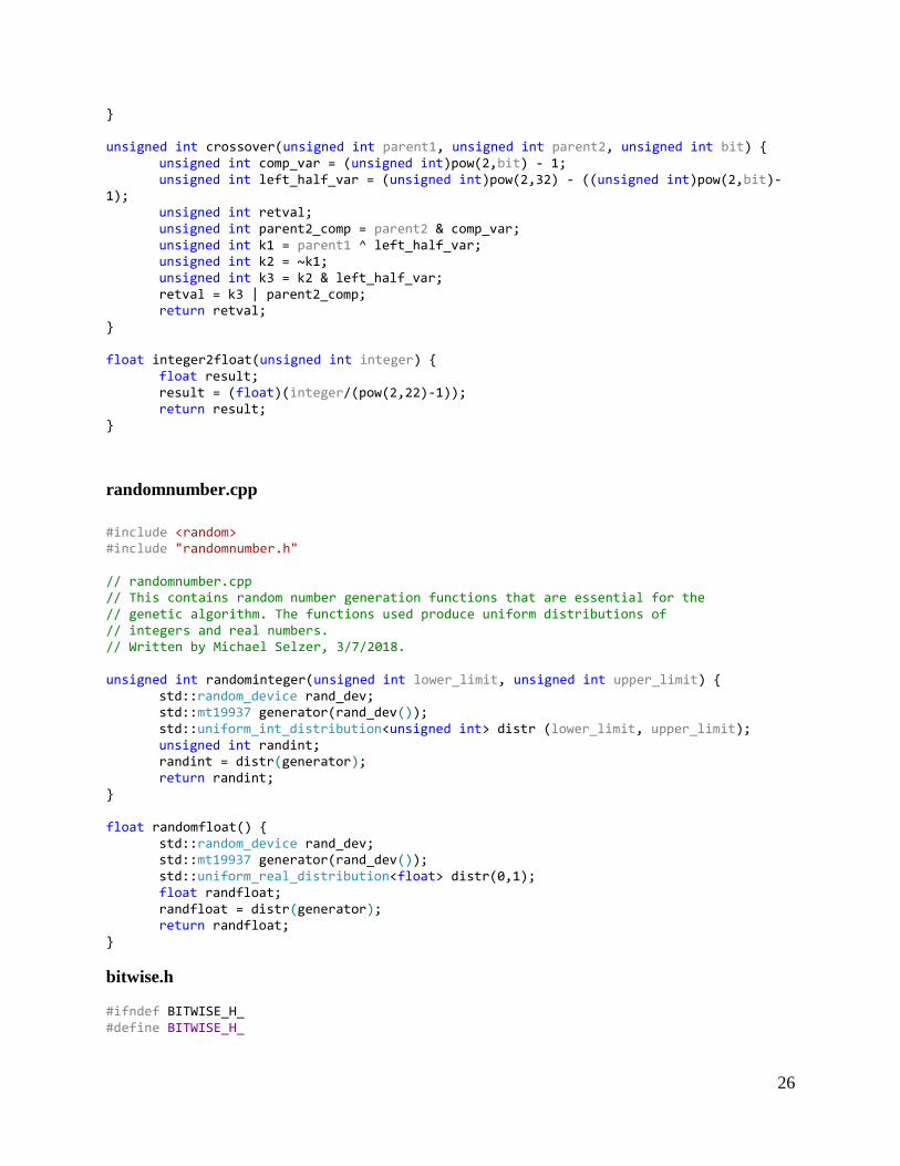
randomnumber.cpp

#include <random> #include "randomnumber.h" // randomnumber.cpp // This contains random number generation functions that are essential for the // genetic algorithm. The functions used produce uniform distributions of // integers and real numbers. // Written by Michael Selzer, 3/7/2018. unsigned int randominteger(unsigned int lower_limit, unsigned int upper_limit) { std::random_device rand_dev; std::mt19937 generator(rand_dev()); std::uniform_int_distribution<unsigned int> distr (lower_limit, upper_limit); unsigned int randint; randint = distr(generator); return randint; } float randomfloat() { std::random_device rand_dev; std::mt19937 generator(rand_dev()); std::uniform_real_distribution<float> distr(0,1); float randfloat; randfloat = distr(generator); return randfloat; }

bitwise.h #ifndef BITWISE_H_ #define BITWISE_H_

27

unsigned int mutate(unsigned int mutatedvar, unsigned int bit); unsigned int crossover(unsigned int parent1, unsigned int parent2, unsigned int bit); float integer2float(unsigned int integer); #endif

randomnumber.h #ifndef RANDOMNUMBER_H_ #define RANDOMNUMBER_H_ unsigned int randominteger(unsigned int lower_limit, unsigned int upper_limit); float randomfloat(); #endif

28

29

Appendix C: Source for the genetic curve fitting program

The genetic curve fitting program can be compiled by running the following command in a

terminal.

make && make clean

Note: bitwise.c, randomnumber.cpp, bitwise.h, and randomnumber.h are unchanged from the test

program. These files are found in Appendix B.

makefile

CFLAGS ?= -g all: gaprogram gaprogram: gaprogram.o objective.o bitwise.o randomnumber.o predictorcorrector2.o singleloop.o predictorcorrector.o successive.o arrhenius.o g++ -g $^ -lm -o $@ gaprogram.o: gaprogram.c g++ -g -c $< -o $@ objective.o: objective.c g++ -g -c $< -o $@ bitwise.o: bitwise.c g++ -g -c $< -o $@ randomnumber.o: randomnumber.cpp g++ -g -c $< -o $@ predictorcorrector2.o: predictorcorrector2.c g++ -g -c $< -o $@ arrhenius.o: arrhenius.c g++ -g -c $< -o $@ singleloop.o: singleloop.c predictorcorrector.o successive.o g++ -g -c $< -o $@ predictorcorrector.o: predictorcorrector.c g++ -g -c $< -o $@ successive.o: successive.c g++ -g -c $< -o $@ clean: rm *.o

gaprogram.c

#include "stdio.h"

30

#include "stdlib.h" #include "string.h" #include "math.h" #include "bitwise.h" #include "randomnumber.h" #include "time.h" #include "objective.h" #include "gaprogram.h" // gaprogram.c // This a test program to ensure that the genetic algorithm in c performs as // expected. This will be transferred into the final program. // Written by Michael Selzer, 3/9/2018. // The current method is based on gaexamplechase.f90 // Differences: // 1. Chromosomes are stored as unsigned integers. Integers are an array of bits. // This allows mutation and crossover to be handled by bitwise operators. // Chromosomes do not require a for loop to convert them into floating point // values. // 2. Random numbers are generated using the uniform distributions in the C++ // <random> library and the Mersenne Twister method. This method is optimized // to handle large series of numbers. // Updates since testga.c // Added dynamic memory allocation for all arrays. This allows n_pop, n_vars, // and n_gen to be specified without recompiling. // Added output file code. // Added input file code. // Changed objective function to the problem, and moved it into objective.c // Created makefile. // Added user interface code. // Modified output file code to fix issues. int n_data = 6; // These can be specified when starting the program. int n_pop = 100; int n_gen = 10000; int n_vars = 4; float p_mut = 0.05; float conv_tol = 1e-8; char inputfile[255]; char outputfile[255]; unsigned int **population; unsigned int **population_old; int fittype = 0; float f_max = 0; float f_min = 1e9; float f_opt = 1e9; float f_sum; float mopt; float *chrom_val = (float *) malloc(n_vars * sizeof(float)); float *calc_val = (float *) malloc(n_pop * sizeof(float)); float i_max; float i_min; float h_sum;

31

float h_i; float *gi = (float *) malloc(n_pop * sizeof(float)); float *v_max = (float *) malloc(n_vars * sizeof(float)); float *v_min = (float *) malloc(n_vars * sizeof(float)); float *v_opt = (float *) malloc(n_vars * sizeof(float)); float convergence=1e7; int mgen = 0; unsigned int *n_rep = (unsigned int *) malloc(n_pop * sizeof(unsigned int)); float *k_reaction = (float *) malloc(n_data * sizeof(float)); float *Tr = (float *) malloc(n_data * sizeof(float)); float *C_Ab_0 = (float *) malloc(n_data * sizeof(float)); float *Pr = (float *) malloc(n_data * sizeof(float)); float *K1r = (float *) malloc(n_data * sizeof(float)); float *C_Aexp = (float *) malloc(n_data * sizeof(float)); float *a_cat = (float *) malloc(n_data * sizeof(float)); float *k_xr = (float *) malloc(n_data * sizeof(float)); void initialize(){ population = (unsigned int **) malloc(n_pop * sizeof(unsigned int *)); population_old = (unsigned int **) malloc(n_pop * sizeof(unsigned int *)); for (int i=0; i<n_pop; i++){ population[i] = (unsigned int *) malloc(n_vars * sizeof(unsigned int)); population_old[i] = (unsigned int *) malloc(n_vars * sizeof(unsigned int)); } for (int i=0; i<n_pop; i++){ for (int j=0; j<n_vars; j++){ population[i][j] = randominteger(0,4194303); // 0 to 2^22-1 } } } void readdata(){ // This may need to be moved to a separate file. int i = 0; char buff[255]; char *variable1; char *variable2; char *variable3; char *variable4; char *variable5; char *variable6; char *variable7; FILE *expdata = fopen(inputfile,"r"); while (fgets(buff, 255,(FILE *)expdata) != NULL){ variable1 = strtok(buff, ","); variable2 = strtok(NULL, ","); variable3 = strtok(NULL, ","); variable4 = strtok(NULL, ","); variable5 = strtok(NULL, ","); variable6 = strtok(NULL, ","); variable7 = strtok(NULL, ","); if (variable1 != NULL) Tr[i] = atof(variable1); if (variable2 != NULL) C_Ab_0[i] = atof(variable2); if (variable3 != NULL) Pr[i] = atof(variable3); if (variable4 != NULL) K1r[i] = atof(variable4); if (variable5 != NULL) C_Aexp[i] = atof(variable5); if (variable6 != NULL) a_cat[i] = atof(variable6); if (variable7 != NULL) k_xr[i] = atof(variable7);

32

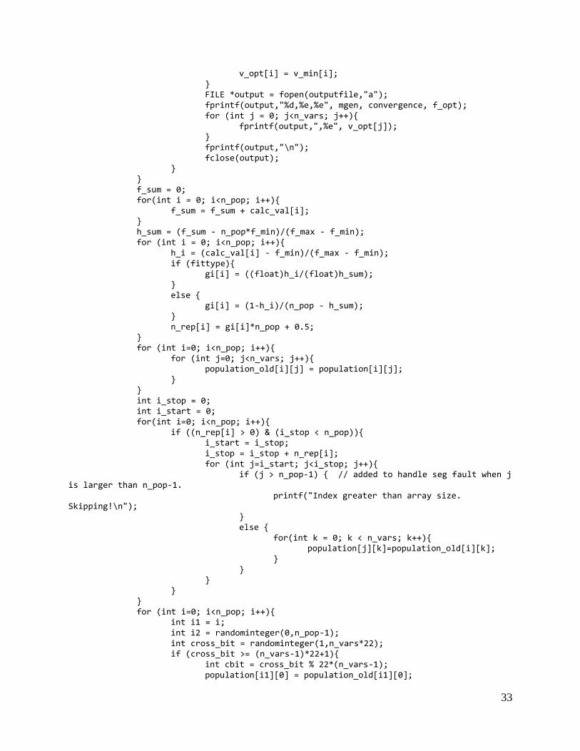
i++; } if (feof((FILE*)expdata)){ printf("End of file.\n"); } fclose(expdata); } void calculate(){ // FILE *output = fopen(outputfile,"w"); clock_t start = clock(); while (convergence > conv_tol){ // for (int g=1; g<n_gen; g++){ mgen++; printf("Generation = %d\n", mgen); for (int i=0; i<n_pop; i++){ for (int j=0; j<n_vars; j++){ chrom_val[j] = integer2float(population[i][j]); } calc_val[i] = function(chrom_val); if (calc_val[i] > f_max) { i_max = i; f_max = calc_val[i]; for (int k=0; k<n_vars; k++){ v_max[k] = chrom_val[k]; } } else if (calc_val[i] < f_min){ i_min = i; f_min = calc_val[i]; for(int k=0; k<n_vars; k++){ v_min[k] = chrom_val[k]; } } } if (fittype){ if (f_max > f_opt) { convergence = (f_max - f_opt)/f_opt/(mgen - mopt); mopt = mgen; f_opt = f_max; for (int i = 0; i<n_vars; i++){ v_opt[i] = v_max[i]; } FILE *output = fopen(outputfile,"a"); fprintf(output, "%d,%e,%e", mgen, convergence, f_opt); for (int j = 0; j<n_vars; j++){ fprintf(output, ",%e", v_opt[j]); } fprintf(output, "\n"); fclose(output); } } else if (!fittype){ if (f_min < f_opt) { convergence = (f_opt - f_min)/f_opt/(mgen - mopt); mopt = mgen; f_opt = f_min; for (int i = 0; i<n_vars; i++){

33

v_opt[i] = v_min[i]; } FILE *output = fopen(outputfile,"a"); fprintf(output,"%d,%e,%e", mgen, convergence, f_opt); for (int j = 0; j<n_vars; j++){ fprintf(output,",%e", v_opt[j]); } fprintf(output,"\n"); fclose(output); } } f_sum = 0; for(int i = 0; i<n_pop; i++){ f_sum = f_sum + calc_val[i]; } h_sum = (f_sum - n_pop*f_min)/(f_max - f_min); for (int i = 0; i<n_pop; i++){ h_i = (calc_val[i] - f_min)/(f_max - f_min); if (fittype){ gi[i] = ((float)h_i/(float)h_sum); } else { gi[i] = (1-h_i)/(n_pop - h_sum); } n_rep[i] = gi[i]*n_pop + 0.5; } for (int i=0; i<n_pop; i++){ for (int j=0; j<n_vars; j++){ population_old[i][j] = population[i][j]; } } int i_stop = 0; int i_start = 0; for(int i=0; i<n_pop; i++){ if ((n_rep[i] > 0) & (i_stop < n_pop)){ i_start = i_stop; i_stop = i_stop + n_rep[i]; for (int j=i_start; j<i_stop; j++){ if (j > n_pop-1) { // added to handle seg fault when j is larger than n_pop-1. printf("Index greater than array size. Skipping!\n"); } else { for(int k = 0; k < n_vars; k++){ population[j][k]=population_old[i][k]; } } } } } for (int i=0; i<n_pop; i++){ int i1 = i; int i2 = randominteger(0,n_pop-1); int cross_bit = randominteger(1,n_vars*22); if (cross_bit >= (n_vars-1)*22+1){ int cbit = cross_bit % 22*(n_vars-1); population[i1][0] = population_old[i1][0];

34

population[i1][1] = population_old[i1][1]; population[i1][2] = population_old[i1][2]; population[i1][3] = crossover(population_old[i1][3],population_old[i2][3],cbit); } else if (cross_bit >= (n_vars-2)*22+1){ int cbit = cross_bit % 22*(n_vars-2); population[i1][0] = population_old[i1][0]; population[i1][1] = population_old[i1][1]; population[i1][2] = crossover(population_old[i1][2],population_old[i2][2],cbit); population[i1][3] = population_old[i2][3]; } else if (cross_bit >= (n_vars-3)*22+1){ int cbit = cross_bit % 22*(n_vars-3); population[i1][0] = population_old[i1][0]; population[i1][1] = crossover(population_old[i1][1],population_old[i2][1],cbit); population[i1][2] = population_old[i2][2]; population[i1][3] = population_old[i2][3]; } else { population[i1][0] = crossover(population_old[i1][0],population_old[i2][0],cross_bit); population[i1][1] = population_old[i2][1]; population[i1][2] = population_old[i2][2]; population[i1][3] = population_old[i2][3]; } } for (int i=0; i<n_pop; i++){ float prob_mutate = randomfloat(); if (prob_mutate < p_mut){ int mbit; int j; int mut_bit = randominteger(1,n_vars*22); if (mut_bit >= (n_vars-1)*22+1){ mbit = mut_bit % (n_vars-1)*22; j = 3; } else if (mut_bit >= (n_vars-2)*22+1){ mbit = mut_bit % (n_vars-2)*22; j = 2; } else if (mut_bit >= (n_vars-3)*22+1){ mbit = mut_bit % (n_vars-3)*22; j = 1; } else { mbit = mut_bit; j = 0; } population[i][j]=mutate(population[i][j],mbit); } } } clock_t end = clock(); double calc_time = (double) (end-start)/CLOCKS_PER_SEC; printf("Calculation time: %lf\n", calc_time);

35

// fclose(output); return; } void menu(); void menu1(); void menu2(); void menu3(); void menu() { int inmenumain = 1; int mainmenu; while (inmenumain){ printf("**************GENETIC ALGORITHM CURVE FITTING PROGRAM*******************\n"); printf(" 1 : Specify input/output file\n"); printf(" 2 : Set GA Parameters\n"); printf(" 3 : Runtime options\n"); printf(" 4 : Run\n"); printf(" 5 : Exit\n"); printf("*********************************************\n"); printf("GAPROGRAM=>"); scanf("%d", &mainmenu); switch (mainmenu){ case 1: menu1(); break; case 2: menu2(); break; case 3: menu3(); break; case 4: initialize(); readdata(); calculate(); break; case 5: inmenumain = 0; break; default: printf("Invalid menu option.\n"); break; } } } void menu1(){ int inmenu1 = 1; int menu1; while (inmenu1){ printf("**********INPUT AND OUTPUT FILES**************\n"); printf(" 1 : Set input file\n"); printf(" 2 : Set output file\n"); printf(" 3 : Set number of data points\n"); printf(" 4 : Return to main menu\n"); printf("**********************************************\n");

36

printf("GAPROGRAM=>"); scanf("%d",&menu1); switch (menu1){ case 1: printf("Enter the full path to the input file: "); scanf("%s", inputfile); break; case 2: printf("Enter the full path to the output file: "); scanf("%s", outputfile); break; case 3: printf("Number of data points: "); scanf("%d", &n_data); break; case 4: inmenu1 = 0; break; default: printf("Invalid menu option.\n"); break; } } } void menu2(){ int inmenu2 = 1; int menu2; int max_search; while (inmenu2){ printf("***********GA PARAMETERS*************\n"); printf(" 1 : Set population size\n"); printf(" 2 : Set number of variables\n"); printf(" 3 : Set fitness type\n"); printf(" 4 : Return to main menu\n"); printf("*************************************\n"); printf("GAPROGRAM=>"); scanf("%d",&menu2); switch (menu2){ case 1: printf("Population size = "); scanf("%d", &n_pop); break; case 2: printf("Number of variables = "); scanf("%d", &n_vars); break; case 3: printf("Searching for maximum? (1/0)"); scanf("%d", &max_search); fittype = max_search; break; case 4: inmenu2 = 0; break; default: printf("Invalid menu option.\n"); break;

37

} } } void menu3(){ int inmenu3 = 1; int menu3; while (inmenu3){ printf("**********RUNTIME OPTIONS***********\n"); printf(" 1 : Set number of generations\n"); printf(" 2 : Set convergence\n"); printf(" 3 : Return to main menu\n"); printf("************************************\n"); printf("GAPROGRAM=>"); scanf("%d",&menu3); switch (menu3){ case 1: printf("Number of generations = "); scanf("%d", &n_gen); break; case 2: printf("Convergence breakpoint = "); scanf("%e", &conv_tol); break; case 3: inmenu3 = 0; break; default: printf("Invalid menu option.\n"); break; } } } int main(){ /* initialize(); readdata(); calculate();*/ menu(); return 0; }

gaprogram.h #ifndef GAPROGRAM_H_ #define GAPROGRAM_H_ extern int n_data; extern float *k_reaction; extern float *Tr; extern float *C_Ab_0; extern float *Pr; extern float *K1r; extern float *C_Aexp; extern float *a_cat; extern float *k_xr;

38

#endif

arrhenius.c #include "math.h" #include "arrhenius.h" // arrhenius.c // Calculates the rate constant for a chemical reaction using the Arrhenius equation. // Written by Michael Selzer, 3/4/2018. double arrhenius(double A, double E, double T){ const double R = 8.314; double k; k = A * exp(-E/(R*T)); return k; }

arrhenius.h #ifndef ARRHENIUS_H_ #define ARRHENIUS_H_ double arrhenius(double A, double E, double T); #endif

objective.c #include "math.h" #include "objective.h" #include "singleloop.h" #include "arrhenius.h" #include "gaprogram.h" #include "predictorcorrector2.h" float function(float parameter[4]) { /*float xmax, xmin, ymax, ymin; xmax = 10; xmin = 0; ymax = 10; ymin = 0; float x = (xmax - xmin)*parameter[0]+xmin; float y = (ymax - ymin)*parameter[1]+ymin; */ float amax, amin, bmax, bmin, Amax, Amin, Emax, Emin; amax = 5; amin = -2; bmax = 4; bmin = -1; Amax = 9; Amin = 3; Emax = 7; Emin = 3; float a = (amax - amin)*parameter[0]+amin; float b = (bmax - bmin)*parameter[1]+bmin; float An = (Amax - Amin)*parameter[2]+Amin;

39

float En = (Emax - Emin)*parameter[3]+Emin; float A = pow(10,An); // input these ranges as 10^n. float E = pow(10,En); float C_Ab, C_Aw, tol, t_f, delta_x, v, Vol; //k_x = 0.076; // mol/m^2*s tol = 1e-8; t_f = 0.102; // m delta_x = 0.00001; v = 0.00036; // m/s Vol = 0.00004; // m^3 C_Ab = 0.15; // these are initial guesses to start the iterative calculation. C_Aw = 0.05; float y_calc[n_data]; float result; for (int i = 0; i<n_data; i++){ k_reaction[i] = a_cat[i] * arrhenius(A, E, Tr[i]); if (i % 4 == 0){ y_calc[i] = predictorcorrector2(C_Ab_0[i], 2, v, Vol, singleloop(k_xr[i], k_reaction[i], a, b, Pr[i], K1r[i], C_Ab, C_Aw, tol, C_Ab_0[i], t_f, delta_x), delta_x); } else { y_calc[i] = predictorcorrector2(y_calc[i-1], 2, v, Vol, singleloop(k_xr[i], k_reaction[i], a, b, Pr[i], K1r[i], C_Ab, C_Aw, tol, C_Ab_0[i], t_f, delta_x), delta_x); } } for (int i = 0; i<n_data; i++){ result = result + pow((C_Aexp[i] - y_calc[i]),2); } return result; }

objective.h #ifndef OBJECTIVE_H_ #define OBJECTIVE_H_ float function(float parameter[4]); #endif

predictorcorrector2.c #include "predictorcorrector2.h" double objective2(double t, double y, double v, double Vol, double C_Ab){ //this is the objective function, f(t,y). double obj; obj = v/Vol*(C_Ab-y); return obj; }

40

double predictor2(double ti, double yi, double v, double Vol, double C_Ab, double delta_x){ // This is the predictor. This step is the Euler's method. double yip; yip = yi + delta_x*objective2(ti,yi,v,Vol,C_Ab); return yip; } double corrector2(double ti, double yi, double v, double Vol, double C_Ab, double delta_x){ // This is the corrector. This corrects the Euler's method solution. double yi1; yi1 = yi + delta_x/2*(objective2(ti,yi,v,Vol,C_Ab)+objective2(ti+delta_x,predictor2(ti,yi,v,Vol,C_Ab,delta_x),v,Vol,C_Ab)); return yi1; } double predictorcorrector2(double y_0, double t_f, double v, double Vol, double C_Ab, double delta_x){ double t_0 = 0; int n = t_f/delta_x; int i = 1; double t_i = t_0; double y_i = corrector2(t_i,y_0,v,Vol,C_Ab,delta_x); for (i = 1; i==n; n++) { t_i = t_i + delta_x; y_i = corrector2(t_i,y_i,v,Vol,C_Ab,delta_x); } return y_i; }

predictorcorrector2.h #ifndef PREDICTORCORRECTOR2_H_ #define PREDICTORCORRECTOR2_H_ double objective2(double t, double y, double v, double Vol, double C_Ab); double predictor2(double ti, double yi, double v, double Vol, double C_Ab, double delta_x); double corrector2(double ti, double yi, double v, double Vol, double C_Ab, double delta_x); double predictorcorrector2(double y_0, double t_f, double v, double Vol, double C_Ab, double delta_x); #endif

singleloop.c #include "predictorcorrector.h" #include "successive.h" #include "math.h" #include "singleloop.h" // singleloop.c

41

// Runs a single loop for one set of inputs. This will be used elsewhere to produce arrays of // calculated C_Ab values at the end of the reactor. // Michael Selzer 3/1/2018 double singleloop(double k_x, double k, double a, double b, double P, double K1, double C_Ab, double C_Aw, double tol, double y_0, double t_f, double delta_x){ double C_Awn1; double C_Abn; double C_Awn = successive(k_x,k,P,C_Ab,C_Aw,a,b,tol); double C_Abl = predictorcorrector(y_0, t_f, K1, C_Awn, delta_x); int i = 0; double convergence = 1e5; while (convergence > tol) { C_Awn1 = C_Awn; C_Abn = C_Abl; C_Awn = successive(k_x,k,P,C_Ab,C_Aw,a,b,tol); C_Abl = predictorcorrector(y_0, t_f, K1, C_Awn, delta_x); convergence = pow(C_Awn - C_Awn1, 2); i++; } return C_Abl; }

singleloop.h #ifndef SINGLELOOP_H_ #define SINGLELOOP_H_ double singleloop(double k_x, double k, double a, double b, double P, double K1, double C_Ab, double C_Aw, double tol, double y_0, double t_f, double delta_x); #endif

predictorcorrector.c #include "predictorcorrector.h" // predictorcorrector.c // This implements the predictor-corrector method in C. // This file can be linked into other code by including predictorcorrector.h // Written by Michael Selzer 2/28/2018. double objective(double t, double y, double K1, double C_Aw){ //this is the objective function, f(t,y). double obj; C_Aw = 0.20; obj = -K1*(y-C_Aw); return obj; } double predictor(double ti, double yi, double K1, double C_Aw, double delta_x){ // This is the predictor. This step is the Euler's method. double yip; yip = yi + delta_x*objective(ti,yi,K1,C_Aw); return yip; }

42

double corrector(double ti, double yi, double K1, double C_Aw, double delta_x){ // This is the corrector. This corrects the Euler's method solution. double yi1; yi1 = yi + delta_x/2*(objective(ti,yi,K1,C_Aw)+objective(ti+delta_x,predictor(ti,yi,K1,C_Aw,delta_x),K1,C_Aw)); return yi1; } double predictorcorrector(double y_0, double t_f, double K1, double C_Aw, double delta_x){ double t_0 = 0; int n = t_f/delta_x; int i = 1; double t_i = t_0; double y_i = corrector(t_i,y_0,K1,C_Aw,delta_x); for (i = 1; i==n; n++) { t_i = t_i + delta_x; y_i = corrector(t_i,y_i,K1,C_Aw,delta_x); } return y_i; }

predictorcorrector.h #ifndef PREDICTORCORRECTOR_H_ #define PREDICTORCORRECTOR_H_ double objective(double t, double y, double K1, double C_Aw); double predictor(double ti, double yi, double K1, double C_Aw, double delta_x); double corrector(double ti, double yi, double K1, double C_Aw, double delta_x); double predictorcorrector(double y_0, double t_f, double K1, double C_Aw, double delta_x); #endif

successive.c #include "successive.h" #include "math.h" // successive.c // This implements the successive substitution step in C. // This can be linked into other code by including successive.h // Written by Michael Selzer 2/28/2018. double successive(double k_x, double k, double P, double C_Ab, double C_Aw, double a, double b, double tol) { double C_Awi; double conv = 1e5; while(conv > tol){ C_Awi = C_Aw; if (b > 1) { C_Aw = pow(k_x/(k*pow(P,a))*(C_Ab-C_Aw), 1/b); }

43

else if (b < 1) { C_Aw = C_Ab - pow(C_Ab, b)*(k*pow(P, a)/k_x); } else if (b == 1) { C_Aw = (k_x*C_Ab)/(k*pow(P,a)*(1+k_x*C_Aw/(k*pow(P,a)))); } conv = pow(C_Aw - C_Awi, 2); } return C_Aw; }

successive.h #ifndef SUCCESSIVE_H_ #define SUCCESSIVE_H_ double successive(double k_x, double k, double P, double C_Ab, double C_Aw, double a, double b, double tol); #endif