Federal Reserve Bank of New York

Staff Reports

Real Estate Investors, the Leverage Cycle,

and the Housing Market Crisis

Andrew Haughwout

Donghoon Lee

Joseph Tracy

Wilbert van der Klaauw

Staff Report no. 514

September 2011

This paper presents preliminary findings and is being distributed to economists

and other interested readers solely to stimulate discussion and elicit comments.

The views expressed in this paper are those of the authors and are not necessarily

reflective of views at the Federal Reserve Bank of New York or the Federal

Reserve System. Any errors or omissions are the responsibility of the authors.

Real Estate Investors, the Leverage Cycle, and the Housing Market Crisis

Andrew Haughwout, Donghoon Lee, Joseph Tracy, and Wilbert van der Klaauw

Federal Reserve Bank of New York Staff Reports, no. 514

September 2011

JEL classification: G21, D18, R31

Abstract

We explore a mostly undocumented but important dimension of the housing market crisis:

the role played by real estate investors. Using unique credit-report data, we document

large increases in the share of purchases, and subsequently delinquencies, by real estate

investors. In states that experienced the largest housing booms and busts, at the peak of

the market almost half of purchase mortgage originations were associated with investors.

In part by apparently misreporting their intentions to occupy the property, investors took

on more leverage, contributing to higher rates of default. Our findings have important

implications for policies designed to address the consequences and recurrence of housing

market bubbles.

Key words: mortgages, leverage

Haughwout, Lee, Tracy, van der Klaauw: Federal Reserve Bank of New York (e-mail:

andrew.haughwout@ny.frb.org, donghoon.lee@ny.frb.org, joseph.tracy@ny.frb.org,

wilbert.vanderklaauw@ny.frb.org). The authors have benefited from helpful comments and

suggestions from participants at the April 2011 Housing Economics and Research Conference at the

University of California, Los Angeles, and the 2011 Society for Economic Dynamics Conference in

Belgium. The views expressed in this paper are those of the authors and do not necessarily reflect

the position of the Federal Reserve Bank of New York or the Federal Reserve System.

 

1 

 

The U.S. economy is still recovering from the financial crisis that began in the fall of 2007.

The collapse of house prices across many markets was a precipitating factor in the financial crisis

and adverse feedback effects between financial markets and the real economy led to the most severe

recession in the post-war period. Extraordinary interventions by fiscal and monetary authorities both

in the U.S. and abroad were required in order to prevent a complete collapse of global markets and

the potential onset of another great depression.

Attention has shifted from containing the financial crisis to examining its causes and

designing policies to limit both the likelihood and the severity of a similar crisis in the future. Given

the central role that housing played as a catalyst to the crisis, it is important to better understand the

determinants of the dynamics of house prices and of subsequent mortgage defaults over this recent

cycle. While house prices were rising in many parts of the country over the period leading up to the

crisis, these increases were particularly pronounced in four states – Arizona, California, Florida and

Nevada (the “bubble” states). Figure 1 shows the path of house prices in the US, the bubble states

as a whole, and in each of these states from 2000 Q1 to 2010 Q4.Over the period from 2000 to 2006

average house prices more than doubled in each of these states. The pace of house price

appreciation accelerated starting in 2004. The peaks in prices across the four states occurred within a

couple of months of each other in mid-2006. Following the turn in the markets, house prices

declined rapidly in each state with much of the earlier gains given back within just two years.2

This rapid run-up and then crash in house prices exacted a terrible cost to homeowners,

financial firms and to the economy. Current estimates are that around 23 percent of active

mortgages are “under water” in that the balance on the mortgage exceeds the current value of the

                                                            2 California is a bit of an exception in that it appears that average house prices have stabilized at a level 50 percent higher than in 2000.

 

2 

 

house.3 As of 2010 Q4, nearly 2.8 million homes have gone through foreclosure, and another 2

million homes are in the process of foreclosure.4 Serious delinquencies continue to add new homes

to the foreclosure pipeline over time. Nationally distress sales represent around half of all repeat-sale

transactions. These distress sales continue to exert downward pressure on house prices making it

more difficult for housing markets to recover.

A focus on residential mortgage finance in order to understand what the determinants were

of the house price and mortgage default dynamics generated over the recent cycle would inform

efforts to enhance financial stability. A more robust system of residential mortgage finance should

aim to limit the degree to which house prices rise and fall over a credit cycle. Reducing the amplitude

of the house price swings will limit the potential for collateral damage created by housing markets

for the real economy.

Related Literature

Given that housing is a durable asset, periods of rising prices are indicative of increasing

demand for housing.5 One strand of the literature on housing demand focuses on the determinants

that affect the “user cost” of housing.6 The user cost of housing (UC) is the annual flow cost to the

owner per dollar of house price, taking into account after-tax financing costs, property taxes and

insurance, maintenance and depreciation costs and the expected risk-adjusted return to owning the

house. The value of the housing service flow is proxied by the annual rent (R). If we assume that

there is arbitrage between owned and rental housing, then the annual rent should equate to the price

of housing (P) times the user-cost.                                                             3 http://www.corelogic.com/About-Us/News/New-CoreLogic-Data-Shows-23-Percent-of-Borrowers-Underwater-with-$750-Billion-Dollars-of-Negative-Equity.aspx 4 http://www.ots.treas.gov/_files/490069.pdf 5 That is, with the exception of natural disasters and periods of armed conflict, the supply of housing in a market cannot contract significantly over a short period of time to drive up house prices. 6 See Hendershott and Slemrod (1983) and Poterba (1984) for early discussions.

 

3 

 

, , , ,

where rm is the mortgage financing rate, τ describes the tax environment, δ the depreciation rate on

housing net of that offset by maintenance expenditures, ge the risk adjusted expected return to

housing, and Y is the average income.

This framework suggests several possible candidates for explaining the rise in house prices in

the early to mid-2000s. A rise in income in a housing market will increase area rental rates to a

degree that reflects the elasticity of supply of rental housing in that local market. Higher rents will

translate into higher house prices by a factor given by the reciprocal of the user-cost in that market.

As a consequence, house prices will vary more with changes in rents in markets with low user-costs

of housing.7 The accommodative monetary policy following the bursting of the tech bubble lowered

mortgage interest rates by over 300 basis points from mid-2001 to mid-2003, and facilitated a

resumption of income growth after the end of the recession .8 Lower financing costs for housing

reduces the user-cost of housing which would lead to higher prices holding rents constant.

However, if some of the benefits of lower financing costs to landlords are passed on to renters, then

the impact of lower mortgage rates on house prices will be attenuated. The Bush tax cuts were

enacted during this period which lowered marginal tax rates. These lower marginal tax rates would

raise the user-cost by reducing the benefit from the mortgage interest deduction. These lower

marginal tax rates would have led to lower house prices, all else the same, with the magnitude of the

reduction reflecting in part expectations over whether the tax cuts would be made permanent.

                                                            7 See Himmelberg et al (2005) for a detailed discussion. 8 http://www.mortgage-x.com/general/historical_rates.asp

 

4 

 

While income, monetary policy and tax rates each underwent some changes in the first half

of the 2000s, the term in the user-cost that has received the most attention in trying to explain the

house price boom is the expected return to housing, ge. The higher the risk-adjusted expected return,

the lower the user-cost and the higher house prices will be in a market. As Himmelberg et al (2005)

explain, the sensitivity of house prices to house price expectations increases with the degree to

which house prices are expected to rise. The expected return to housing is the only forward-looking

aspect to the user-cost of housing framework. The arbitrage condition listed above has a potential

self-fulfilling characteristic. If owners expect house prices to rise in the future, then the user-cost of

housing will fall and, given a constant rent, the value of houses will rise.9 This rise in the value of

housing can serve to confirm the earlier belief. This may lead to “irrational exuberance” in the

housing market as argued by Shiller (2005).

Himmelberg et al (2005) apply the user-cost formulation to assess the degree to which house

prices dynamics track changes in fundamental demand determinants for housing. They calculate

user-cost estimates for 46 metropolitan areas over a twenty-five year period ending in 2004. Their

analysis identified only a few metropolitan areas where by 2004 house prices appeared to have risen

significantly more than what would be predicted by average rents and estimated user-costs. It is

unfortunate that their analysis ended in 2004 since the rapid acceleration in house price appreciation

as shown in Figure 1 began in that year. Given their argument that the sensitivity of prices to user-

costs increases at low values of the user-cost, it is possible that their methodology if extended

through 2006 would have explained some of this acceleration in price appreciation. However, it is

important to note that the average 30-year fixed-rate mortgage rate increased from 5.74 in January

                                                            9 Rents would not be expected to rise since the value of the current flow of housing services has not changed.

 

5 

 

2004 to 6.14 in December 2006, so that any further declines in the user-cost was not being driven by

lower financing costs during this period.10

Glaeser et al (2010) argue that the empirical connection between mortgage rates and house

prices is not strong enough to explain the dynamics of house prices during the housing boom. On a

conceptual level, they argue that the impact of any shift in housing demand on house prices depends

on the housing supply elasticity in that market. For markets with inelastic housing supply, increases

in housing demand will mainly result in higher house prices instead of increased production of new

homes. In contrast, in housing markets with elastic housing supply, increases in housing demand will

mainly result in the production of new homes. House prices in these markets are determined by the

cost of building a new home.11 Furthermore, they argue that expected future mortgage rates are

important in addition to the current mortgage rate. If mortgage rates are expected to rise, then the

effect of a low current mortgage rate on house prices will be attenuated. This argument can be

captured in the user-cost arbitrage condition shown earlier by factoring the expected rise in

financing costs into the expected house price appreciation term.12

Credit conditions enter into the standard user-cost formulation solely through the mortgage

interest rate. However, a second important aspect is the required downpayment by the borrower.

The interest rate and the required downpayment reflect the two underwriting constraints on a

borrower when bidding on a property. The minimum downpayment percentage is also referred to as

the “collateral rate” on the mortgage.13 For a given mortgage balance, the mortgage interest rate

impacts the monthly payment that the borrower will have to make. Underwriting standards will

                                                            10 Some authors pointed to the rise in price-rent ratios as likely to be followed by a reduction in subsequent price growth (Gallin 2008, Campbell, et al. 2009). 11 See Glaeser et al (2010) for a detailed discussion. 12 An implication is that a reduction in interest rates that is perceived to be permanent would be expected to have a greater impact on house prices than a similar reduction in interest rates that is due to accommodative monetary policy and is expected to be transitory. This presents a challenge to those who hold the view that monetary policy was a primary determinant of the house price boom. 13 The collateral rate is also referred to as the “haircut” or “margin.”

 

6 

 

stipulate a maximum that the sum of the annual mortgage payments in addition to the taxes and

insurance on the property can be as a fraction of the borrower’s income.14 We will refer to this as the

“cash-flow constraint”. A lender will also require the borrower(s) to make a minimum

downpayment. The ratio of the downpayment to the sale or appraised value of the house determines

the origination loan-to-value ratio (LTV). We refer to this as the “downpayment constraint.” The

maximum that a borrower may bid on a house will depend on which of these two constraints first

becomes binding given the underwriting standards in use at the time.

The mortgage interest rate and the collateral rate are jointly determined in a credit market

(see Fostel and Geanakoplos (2008) and Geanakoplos (2009)). For collateralized loans the collateral

rate is determined by volatility of the asset price and the term of the loan. The higher the price

volatility and the longer the term, the larger the collateral rate the lender will require (or equivalently

the larger the minimum downpayment percentage). The purpose of the collateral rate is to safeguard

the lender against defaults by the borrower when there are declines in the value of the collateral.

Similarly, for a given level of price volatility, the higher the expected price appreciation for the asset

the lower lenders may set the required collateral rate. In this case, the expected price appreciation

acts as additional future collateral protecting the lender against losses in the event of a default.

There is an additional channel, not necessarily captured by changes in the average origination

LTV and not explicitly addressed by Glaeser et al (2010), through which changes in credit conditions

may have affected housing prices. Reduced loan documentation requirements may allow those who

previously hit the collateral or cash-flow constraint to obtain more leverage, be it possibly at less

favorable terms. This could occur when lenders no longer require income documentation or adopt

more favorable ways of imputing the borrower’s future income from wage earnings, bonuses and

                                                            14 This is the called the front-end PITI (for principal, interest, taxes and insurance as a fraction of income) or DTI (debt-to-income ratio). There is also a back-end ratio that adds to the numerator any recurring non-housing debt payments such as auto loans, student loans, and minimum credit card payments.

 

7 

 

possibly rental income. Alternatively, in computing the DTI ratio, debts other than the mortgage

loan under consideration may be ignored or incorporated differently.

As shown in Table 1, significant changes in documentation requirements for subprime and

Alt-A loans took place during the run-up in house prices. The level of documentation for a new

mortgage is reported as a data item on the origination file for that mortgage. The three values are full

documentation, limited documentation and no documentation. While no-doc loans remained

relatively uncommon, there was a sizeable shift from full-doc to low-doc loans for subprime and

especially for Alt-A mortgage loans. By 2006 some 38% of newly originated subprime and 81% of

new Alt-A loans were low- or no-doc loans.

We can incorporate changes in underwriting standards into the user-cost framework.

, , , , ,

where LTVM is the maximum allowed origination loan-to-value ratio, s captures other prevailing

underwriting standards at the time of the home purchase such as DTI and documentation, and f

captures how changes in the degree of leverage and documentation impact house prices holding

constant the user-cost.

Finally, there is a potentially important amplification effect of leverage on house prices

which is not fully captured in our augmented user-cost arbitrage conditions. Geanakoplos (2009)

posits that there is not a common house price appreciation expectation, ge, that is shared by all

potential buyers of an asset. Rather, he starts with the assumption that there is a distribution of

expected appreciation rates across potential buyers. At the high end of the distribution are

“optimistic” potential buyers with high values of ge. Holding constant all of the other factors in our

 

8 

 

user-cost arbitrage condition, optimistic buyers will be willing to bid higher prices for housing since

their user-costs are lower.

This distribution of buyers in terms of their opinions about the future value of housing can

generate an amplification mechanism for house price dynamics. In normal times, optimistic buyers

are infra-marginal participants in the housing market. At the prevailing house prices they would like

to purchase additional housing but are prevented from doing so because the cash-flow constraint or

the downpayment constraint is binding. However, during the early phase of a housing boom, lenders

may reduce the required downpayment percentage on new mortgages and begin to relax other

underwriting standards due to the strong performance of house prices and low delinquency rates.

These actions enable the optimistic buyers to purchase additional housing. The increasing leverage

allowed in the market, then, begins to shift the composition of new purchase transactions in the

market toward more optimistic buyers who are willing to bid higher prices for houses. This is an

additional channel by which higher leverage can amplify the upward pressure on house prices.

Geanakoplos describes this dynamic as the upswing phase of a “leverage cycle”.

Can increasing leverage help to explain the acceleration in house prices from 2004 to 2006?

For leverage to have played an important role we need to establish at least two things. First, we need

to show that leverage was increasing over these three years. Second, we need to demonstrate that the

composition of purchasing activity was shifting toward more optimistic buyers. Table 2 summarizes

changes in leverage from two different sources of information on housing transactions and

mortgages. Glaeser et al (2010) report data on combined LTV ratios for purchases drawn from 89

metro areas and recorded by DataQuick. An advantage of this data is that they reflect all mortgage

products that were used to finance these purchases and reflect up to three liens on the house. The

 

9 

 

second is changes in leverage on securitized nonprime purchase mortgages as recorded by

LoanPerformance.15

There are two observations that can be drawn from Table 2. First, as pointed out in Glaeser

et al (2010) extreme leverage in the form of zero downpayment mortgages were available and used

by at least 10 percent of borrowers.16 Second, when we look below the 90th percentile, we see that

leverage was increasing throughout the distribution of origination LTVs.17 Glaeser et at (2010),

however, conclude that the magnitude of the observed LTV changes do not appear to be large

enough to be an important determinant of the acceleration in house prices. This conclusion may be

model dependent. If Geanakoplos (2009) is correct that increasing leverage also affects prices

through shifting the composition of buyers, then this additional amplification mechanism may imply

that the observed changes in leverage are capable of explaining more of the acceleration in house

prices. Glaeser et al (2010) in fact explicitly condition their conclusion (that credit market factors

were not the main drivers of the housing boom) on the absence of significant composition changes

in the population of buyers. They also raise the distinct possibility that the surge in the number of

buyers during the boom may have been accompanied by an overall decline in credit quality of buyers

not captured by LTVs, but were not able to find any evidence of large composition changes when

measured by demographics.

One such potential shift in the composition of buyers during the housing boom and

especially during the 2004-2006 period, concerns the number and activities of real estate investors.

There are several reasons to expect credit conditions to have particularly affected investor activity in

                                                            15 Our finding of increases in the median nonprime CLTV at origination is consistent with that of Mayer and Pence (2009). We use our matched sample, which represents a random sample of all LP loans as described below, for this table. 16 The Glaeser et al (2010) data indicate that the 90th percentile was at 100 going back to 1998. 17 This is consistent with trends reported by Geanakoplos (2009, chart 1) for the average downpayment as a proportion of the purchase price. Among the 50% lowest downpayment ratios for subprime and ALT-A borrowers (based on CoreLogic data), he found a decrease in the average downpayment from 13% in the first quarter of 2000, to a low point of 2.7% in the second quarter of 2006.

 

10 

 

the buildup of the housing boom. In discussing these, we will distinguish between three different

types of buyers in a housing market: buyers who want to live in the house (owner-occupiers),

investors who want to keep the house as vacation or future retirement home or who want to rent

the property and then resell at a future date (buy and hold), and investors who want to resell the

property without living in or renting the house (buy and flip).

The first reason to expect a role for investors in bidding up prices concerns the impact of

the previously discussed increase in average origination LTVs. For a given mortgage interest rate,

reducing the required downpayment percentage can allow a borrower to bid more aggressively for a

property, but this is especially so for investors. The easiest way to see the impact of variation in the

allowed LTV on the maximum bid is to take the case of a “buy and flip” borrower. As an

illustration, consider an investor who has $50,000 to invest in real estate. This money must cover the

downpayment as well as the mortgage payments, property taxes and home insurance during the

expected holding period. For simplicity, we assume that the house is financed with a 30-year fixed-

rate mortgage with an interest rate of 5.5 percent. We assume that annual property taxes, insurance

payments and any required maintenance expenditures equate to 2 percent of the house value. The

investor will not be renting out the property during the time until resale. We consider two cases: in

the first the investor plans to be able to finance the purchase for up to three years, and in the second

the investor plans to be able to finance the project for up to two years.

The relationship between the allowed level of leverage as indicated by the origination LTV

and the maximum bid is shown in Figure 2. For the three year holding horizon, the maximum bid

increases from $118 thousand with a twenty percent downpayment requirement to $189 thousand

with no downpayment required – a sixty percent increase. The sensitivity of the maximum bid to

 

11 

 

changes in the origination LTV is increasing in the degree of leverage.18 For example, reducing the

required downpayment from 20 percent to 19 percent raises the maximum bid by $2,260. Reducing

the required downpayment from 5 percent to 4 percent raises the maximum bid by $4,189 – nearly

double the earlier increase. For the same degree of leverage, investors with a shorter holding period

have a higher maximum bid. We show how the schedule of maximum bids increases as the investor

moves from a three to a two-year holding period. Shorter holding periods also increase the

sensitivity of the maximum bid to changes in leverage at any given LTV. For example, with a two

year holding period moving from a 5 percent to a 4 percent required downpayment raises the

maximum bid by $9,335. Investors may have shortened their expected holding periods as the

housing market heated up and the pace of house price increases accelerated. For a given maximum

leverage, faster turn-around times for the investment properties would allow the investors to bid

more aggressively.

A second mechanism through which investor behavior may have amplified the impact of

changing credit conditions on house prices is through the loosening of loan documentation

requirements. It has been speculated that the loosening of documentation standards may have

facilitated the misreporting by borrowers of their true expected home-occupancy status.19 This in

turn may have enabled them to purchase homes under more favorable terms than they would have

as investor. We explore the evidence for this possibility below.

A third channel affecting real estate investors concerns the use of second liens on existing

mortgages to facilitate the down payment and meeting of loan requirements for purchasing

additional investment properties. As documented in earlier work by Chakrabarti et al (2011), with

house prices appreciating homeowners extracted home equity through higher balances on first

                                                            18 The nonlinearity is due to the fact that the origination LTV is determined by the ratio of the downpayment to the value of the house, which here equals the maximum house bid. 19 See, for example, http://www.fincen.gov/news_room/rp/reports/html/mortgage_fraud112006.html.

 

12 

 

mortgages, cash-out refinances, second mortgages and home equity lines of credit. In fact, on

average for each 1% increase in home prices, homeowners increased their mortgage debt by 1%, so

that proportionally their equity share in their homes actually remained relatively constant until the

end of 2006. Equity extraction may have been especially attractive to optimistic, but cash-

constrained investors, by allowing them to use these funds to make downpayments on purchases of

additional homes. Accordingly, we expect the combined LTV on existing mortgages to have

increased for investors during the period in which they purchased additional properties.

Finally, we refer again to the amplification effects that result from shifts in the market

toward more optimistic buyers. In the next section of the paper we explore the Geanakoplos

hypothesis. We identify optimistic buyers as investors, and especially the “buy and flip” investors.

We document the role of this class of investors over the past credit cycle both nationally as well in

four boom states. We explore the extent to which the investor share of purchase transactions

changes over the credit cycle. These changes are decomposed into both the extensive margin – more

investors enter the market – and the intensive margin – existing investors increase the size of their

portfolio of residential real estate exposures. We also examine the default behavior of investors as

compared to owner-occupant borrowers. The final section of the paper discusses implications of our

findings for current policy work on improving financial stability.

Investors and the Leverage Cycle

If Geanakoplos’ description of the dynamics of the leverage cycle is applicable to the

housing boom-bust cycle of the 2000s, we would expect to see changes in the characteristics of

leveraged buyers of residential real estate over the period. In this section, we provide descriptive

evidence of some major changes in the observable characteristics of mortgagors between 2000 and

2010.

 

13 

 

While there has been some anecdotal evidence supporting the idea that investors played an

important role in the boom, careful analysis of this issue has been impeded by lack of appropriate

data.20 For investors, the benefits of living in a house are immaterial to the decision of whether or

not to keep making the mortgage payment, making default a less costly decision for investors than

for owner-occupants. Of course, lenders are well aware of this difference, and typically require

mortgagors to declare whether they will live in the collateral property, charging higher interest rates

and requiring higher downpayments from those who acknowledge that they will not, ceteris paribus.

But the interest rate penalty and limitations on leverage discourage borrowers from declaring their

intention to live elsewhere, and self-reported “occupancy status” is thus considered a particularly

unreliable piece of data. Haughwout et al (2008), for example, indicate their suspicion that miscoding

of occupancy status in loan-level data may help to explain the large increase in early nonprime

defaults that are unexplained by observable – i.e., reported - characteristics of loans and borrowers.21

Fitch (2007) found evidence of occupancy misrepresentation in two-thirds of the small sample of

subprime defaults they examined. It is thus desirable to identify a mortgage data source that allows

the analysis of borrowers without relying on the information that is self-reported by the borrower on

the mortgage application.

We bring two distinct kinds of data to the analysis of this important question. Our primary

source is the FRBNY Consumer Credit Panel (CCP) which comprises an anonymous and nationally

representative 5% random sample of US individuals with credit files and all of the household

members of those 5%. 22 In all, the data set includes files for more than 15% of the population, or

                                                            20 See, for example, http://www.metrotrends.org/commentary/mortgage-lending.cfm 21 Early defaults are defined to be defaults that occur within the first year. 22 The FRBNY CCP panel is based on Equifax credit report data. Lee and van der Klaauw (2010) provides further details on the data set. The analyses reported in this paper are solely based on the representative random sample and do not include the additional household members sampled.

 

14 

 

approximately 37 million individuals in each quarter from 1999-2011Q1.23 The FRBNY CCP data

allow us to overcome some of the difficulties with self-reported occupancy status. Unlike loan-level

data, which focus on individual debt contracts and the information used in underwriting them, credit

reports are designed to give lenders (and potential lenders) dynamic credit information on individual

borrowers, including the types and amounts of debt they have outstanding at any point in time. Our

panel allows us to track individual borrowers over time, through refinances and moves, where at

each point in time we observe all outstanding mortgage loans and non-mortgage debts.

We can use this information to separate mortgage borrowers based on how many distinct

first-lien mortgage accounts appear on their credit reports. Since each property can secure at most a

single first-lien mortgage, the number of such mortgages on a borrower’s credit report is a reliable,

non-self reported, indicator of the minimum number of properties a given individual has borrowed

against.24 This kind of information about individual borrowers is not available in loan-level data sets

and thus the FRBNY CCP data provide a unique perspective into important questions about who is

originating new mortgages at any point in time, as well as their subsequent behavior.

At this point, it is worth extending our earlier discussion of the relationship between the

number of properties against which an individual has levered and what Geanakoplos describes in his

leverage cycle theory. First, it is important to note that virtually all homeowners have some

investment motivation in making a home purchase. While there is some debate in the academic

literature about whether housing is a good investment relative to other assets, many buyers –

whether they own only the home in which they live or own several units at a time – consider

                                                            23 In the balance of the paper, we use the term “mortgages” to refer to installment debt secured by residential real estate. Mortgage payments are typically determined so as to pay off the balance, plus interest, over a fixed time period, but some mortgages negatively amortize – the balance can grow over time. HELOCs are lines of credit, again with residential real estate as the collateral. HELOC borrowers may utilize credit up to some fixed limit. 24 Because some properties may have no first-lien mortgages but do secure a HELOC, our count of properties is a minimum rather than an exact figure. In addition, some properties support no debt at all.

 

15 

 

expected capital gains a part of their motivation for buying rather than renting (Case and Shiller

1988). However, some homebuyers differ from others in that some or all of their residential

property portfolio does not also directly provide them with shelter: that is, they own multiple

properties and do not live in all of them. While we recognize the investment motive of all

homeowners, we will refer to these multiple property owners as “investors”. Regardless of what

these borrowers are called, the data make clear that they act differently from other housing market

participants, as we shall see below.

As we suggested above, some further differentiation among investors is in order. On the one

hand, there exists a class of borrowers who buy properties in order to rent the housing units they

contain. For these investors, the flow of rental income generated by real property is an important

motivation for their investment, and the crucial consideration, as described above, is whether this

income exceeds the cost of carrying the property (roughly speaking, principal, interest, taxes,

insurance, maintenance net of any tax considerations) over a long period of time. Other investors

may buy properties to use as a vacation or future retirement home. These “buy and hold” investors

will thus be sensitive to changes in interest rates: a significant decline in rates can often offset the

fixed cost of refinancing since they expect to hold the property for some time.

By comparison, the kind of investors portrayed in the popular television show “Flip This

House” differs from those who hold assets for their income-generating potential. Indeed, in that

program, a team of investors typically purchases a house, does some renovations and then re-sells

the property to a new owner without ever receiving any rental income whatsoever. For these “buy

and flip” investors, the primary motivation for the investment is capital gains, suggesting, for the

reasons described above, that they will be both highly leveraged and will be considerably less

sensitive to interest rate movements. In what follows, we will explore several dimensions of the

behavior of investors in general, using the data on multiple first-lien mortgages as a way of

 

16 

 

distinguishing investors from owner-occupants. In our analysis we will distinguish between different

categories of investors; by whether they are holding 2, 3 or 4 or more first mortgages. It is more

difficult in our data to differentiate investor type – flippers vs. holders – within each category,

although changes in many of the investor series as the boom unfolds are strongly suggestive of a

change in composition of the investor group, as we shall see.25

While the CCP data provides unique insights into the role of investors in the entire mortgage

marketplace, it has some limitations. A specific drawback is the absence of information about the

collateral property – its location and value – in the credit report data. To allow additional analyses,

we have matched individual mortgage loans from the CCP data to loan-level data from CoreLogic’s

LoanPerformance ABS database. LoanPerformance ABS data provides detailed loan-level

information on over 15 million securitized nonprime loans, including loans which were packaged

into subprime and “Alt-a” private label securities, but excluding jumbo loans with balances that

exceed the GSEs’ conforming limits. The LoanPerformance (LP) data include detailed information

on both the origination characteristics of the loans – such as level of documentation, interest rates,

balance, and the value and location of the collateral property.26 Interestingly, the data also include

the borrower’s self-reported occupancy intentions: indicating whether the property’s purpose will be

for owner-occupancy, for use as a second home, or for an investment property, which we can

compare with our own definition of investors: CCP information on the number of first-liens

                                                            25 Ex post we can differentiate by the average holding periods by different investors. However, the preferred classification would be based on the ex ante expected holding periods which we do not observe. Bayer et al (2011) use the former approach, defining flippers by the number of times they bought and sold a home in less than two years during the 1992-2005 period in Los Angeles. They then refer to individuals with two or three flips during the period as speculators, and those with over 10 flips as middlemen. 26 Our merge was provided by Equifax Corporation using servicers’ loan numbering system. Given that the CCP constitutes a representative random sample of individuals, the matched sample represents a representative random sample of LP loans.

 

17 

 

reported contemporaneously on the borrower’s credit report. 27 We will contrast the data on these

“investor” definitions below; for now it is worth pointing out that the mortgage application refers to

the reported use of a particular property, while the credit report refers to the extent of residential

investment by an individual.

Our matched data are, of course, reflective of a subset of the entire market, albeit the part

that changed most rapidly and noticeably during the boom. Even with the matched data, we are

limited to analysis of individuals’ credit reports: to the extent that residential real estate investment is

conducted through incorporated businesses or partnerships, we will not capture that form of

investor activity here. Notwithstanding these limitations, the FRBNY CCP and our matched dataset

provides many unique benefits that will allow a much clearer picture of the kinds of borrowers

holding, originating and defaulting on mortgages during the 2000s housing cycle. Moreover, the

matched data overcome many of the limitations of the datasets used in isolation, and allow us to

examine both the characteristics of the loans and details of the borrower’s credit report

simultaneously.28

Results

We begin by using the CCP data to provide a description of the part played by various types

of buyers in the stock of outstanding mortgages. A fundamental stylized fact from the Geanakoplos

model is that investors in their role as optimistic buyers ought to be playing an increasingly

                                                            27 An alternative definition would define investors in a more static way, by identifying individuals who at any point in our sample period had more than one first-lien mortgage on their credit reports. Using that definition, our primary results remain similar to those reported here, although we discuss this distinction further below. 28 We observe borrowers’ credit reports on the final day of each quarter. Because there can be delays in credit reporting such that a mortgage that has been paid off may stay on the credit report for a period of time, we use the data’s panel structure to correct for these delays. Throughout this section of our analysis investor status is determined based on the maximum number of first mortgages that appear in both of the two most recent quarters. Thus we can be more confident that each first-lien we consider is in fact associated with a unique property.

 

18 

 

important role in borrowing during the upswing in the leverage cycle. Figure 3(a) shows the

proportion of all new purchase mortgage balances originated by borrowers with 2, 3 and 4 or more

first-lien mortgages on their credit reports in each quarter between 1999Q1 and 2010Q4. As can be

seen in the figure, this investor proportion increased from around 20 percent in 2000 to a peak of

nearly 35 percent in 2006. The purchase share for borrowers with 4+ first-lien mortgages increased

by more than 5 percentage points over this period. Meanwhile, investors make up a much smaller

share of refinance originations (see Figure 3(b)), a result consistent with the view that investors hold

properties for shorter periods.29 For borrowers with short time horizons, the fixed costs of

refinancing can make the option to refinance uneconomic.

Previous research has indicated that there was significant variation in the timing and, most

importantly, the amplitude of the housing cycle over space (see, for example, Himmelberg et al

2005). If investors were playing an important role in fueling the growth of house prices in those

states which experienced the greatest increases, we would expect to see differences over space in

investors’ share of the mortgage market. Our data confirm this conjecture. Figure 3(c) displays the

same information focusing on the four states that experienced an especially pronounced housing

cycle: Arizona, California, Florida and Nevada. Multiple lien holders of all types (2, 3, and 4+) were

more prevalent in these “bubble” states than they are for the nation as a whole. The investor share

of purchase mortgages also increased faster in these states as the housing boom peaked, rising from

almost 25 percent in 2000 to 45 percent in 2006. The purchase share for borrowers with 4+ first-lien

mortgages increased by more than 7 percentage points (or 350%) over this period.

                                                            29 Unlike loan-level data, borrower-level credit report data indicates the closing and opening of mortgage loans over time but do not include an indicator for whether a new mortgage loan represents a new purchase origination or a refinance. We identify refinances as a closing and opening of a new mortgage loan within a 6 month period during which the loan holder did not change address. Our refinance measure therefore may include some purchase loans associated with cases where an investor sold and bought a new property within a relatively short period of time. Nonetheless as shown later the patterns displayed in Figure 3 are mirrored in our matched sample, where loan purpose (purchase vs refinance) is explicitly measured. See Figure 7.

 

19 

 

Given this evolution of the flow of mortgage borrowing, it is unsurprising that we find

investors increasing their share in the stock of mortgage debts. Figure 4(a), shows the share of

outstanding mortgage balances owed by the number of first-liens reported on the borrowers’ credit

report. 30 Beginning in 2004, we see a pick-up in the share of all mortgage debt owed by borrowers

with multiple first-liens, and this figure reached 24.7% by early 2008. Figure 4(b) displays the same

information for the four “bubble” states. At the peak nearly one-third of all first-lien balances in

these four states were owed by borrowers with at least two first-liens. By the peak in early 2008,

first-lien mortgage debts owed by bubble state borrowers with four or more first-liens had risen to

nearly $170 billion, over three and a half times their levels of early 2004. Figure 5 shows the investor

share over time by selected states. For all states listed, their share of mortgage balances increases

over the boom but with less amplitude than in the bubble states.

In the upswing phase of a leverage cycle that is unfolding as described by Geanakoplos, we

would expect to see increases in both the extensive margin (reflected here as increases in the share

of buyers who have multiple first-liens) and in the intensive margin (increases in the number of first-

liens held, conditional on having more than one and increases in the average balances for each

mortgage). The data demonstrate both increasing prevalence of investors in the housing marketplace

and an increase in their share of outstanding and newly originated debt. An increased share of

borrowers with multiple first-liens is evidence of an increase in the extensive margin: investor status

became more widespread during the boom, especially in those markets where prices rose the most

sharply. The fact that the share of new and existing purchase mortgages were owed by investors

                                                            30 Between 2004Q1 and 2008Q1 the share of borrowers who had multiple first-liens increased from 7.3% to nearly 10%. During this four year period, the share of all mortgage borrowers with four or more first-lien mortgages on their credit reports increased by more than 50% (from 0.43% to 0.70%). In bubble states the investor share increased from 10% to 14% during this period, while the share of borrowers with four or more first-liens increased from 0.65% to 1.22%

 

20 

 

reflects this fact, but also may reflect the intensive margin, as investor-types increased their exposure

to the housing market by borrowing more against residential property.

In order to discriminate between the two, we examine the intensive margin more carefully.

In Table 3, we show the average balances on mortgages owed by the number of first-liens reported

on the borrower’s credit report for the US and the bubble states. We observe a change in the relative

size of first-liens owed by highly leveraged borrowers. Because property values were rising sharply

between 2000 and 2006, it is no surprise that the average balance on outstanding first-lien mortgages

rose as well. But balances owed by investors rose even more sharply than those owed by owner-

occupants. In 1999 for the US as a whole (panel (a) of Table 3), the average balance on first-liens

owed by borrowers with debt secured by more than three properties was 13% higher than that of

owner-occupants.31 By 2006, the average investor balance (in the 4+ line) was nearly 50% larger than

the corresponding owner-occupant figure. Interestingly, a more muted version of the same pattern

obtains in the bubble states, shown in panel (b).

Further evidence of this increase in the intensive margin is found in Figure 6. Here we track

the transitions into and out of the various first-lien mortgage count categories. In both panels (a)

and (b) we find what we will refer to as “up-leveraging” transitions: the proportion of investors in

year t-1 who have additional mortgages in t.32 For example, Figure 6(a) shows that approximately 6%

of all investors with two first-lien mortgages in 2005 had added a third by 2006. As can easily be

seen in the figure, the proportion of all mortgage borrowers who added additional properties to their

portfolios grew between 2000 and 2006, with the sharpest increases found among those who already

had the highest residential real estate holdings. Around 12% of US borrowers with exactly three

                                                            31 A similar relative increase is observed for average origination balances. 32 The transition rates are based on the maximum number of first mortgages held during the two most recent quarters at time t, and the maximum number of first mortgages held during the two most recent quarters at time t-1.

 

21 

 

first-liens in 2005 added additional properties to their portfolios during 2006; in the bubble states

this figure exceeded 16%.

We conclude from our analysis that mortgage borrowing by investors – defined as those

with multiple properties in their portfolios – increased substantially during the boom, especially in

those markets where house price increases were particularly pronounced. We find evidence of

increases in both the extensive margin – new investors entering the marketplace – and the intensive

margin – increased exposure to residential real estate among previous investors.

These results contrast with previous discussions of the role of investors in the mortgage

marketplace, and underscore the benefits of the FRBNY CCP for analyzing these questions. Mayer,

Pence and Sherlund (2008), for example, conclude “because our data show that [self-identified]

investors were a small or declining share of overall originations [of non-prime mortgages], it seems

unlikely that they accounted for much of the rise in the overall delinquency rate unless they increasingly

misrepresented themselves as owner-occupiers or their unobserved characteristics deteriorated over time.”

(2009, pg. 44, emphasis added). Our data allow us to “see through” the self-reported information

captured on the mortgage application, and show precisely this – an increasingly large discrepancy

between mortgage application occupancy self-reports and the number of first-liens on the credit

report during the crucial 2004-2006 period. These results thus leave open the question of the role of

these investors in the subsequent increase in defaults and delinquencies.

Figure 7 contains three panels which explore the relationship between occupancy self-

reporting on mortgage applications and borrowers’ first-lien counts for our matched CCP-LP

sample. In panel (a), we plot the proportion of new nonprime purchase originations by self-reported

occupancy status (from LP) and number of first-liens (from CCP). The dashed line plots the

proportion of balances taken out by borrowers who checked either “2nd home” or “investor

property” on the mortgage application, while the solid line shows the proportion of balances

 

22 

 

originated by these same borrowers who, after closing this mortgage, simultaneously have two or

more first-liens.33

Comparing the two series provides some insight into the value of self-reported occupancy

status. First, at the beginning of the period the two series are reasonably close together, but even in

2000 there is a significant discrepancy between what borrowers report on the mortgage application

and the number of properties they own. Over time, the proportion of new originations by

borrowers who acknowledge that they will not use the home as their primary residence (the dashed

line) increases slowly, and is fairly flat at 13-15% for the crucial 2004-2006 vintages. While we are

including second homes, balance weighting and using only purchase mortgages, this pattern is

similar to the results found by Mayer, Pence and Sherlund (2008). Meanwhile, however, the

proportion of borrowers who have 2 or more first-lien mortgages rises much more quickly, and

approaches 41% by 2006. The bubble states, shown in Figure 7(b), exhibit the same pattern,

although in somewhat more extreme, where in 2006 the gap between self-reported occupancy status

and the number of first-liens reached 30 percentage points. In other words, many of the borrowers

who claimed on the mortgage application that they planned to live in the property they were

purchasing had multiple first-lien mortgages when the transaction was complete. Mayer, Pence and

Sherlund (2008) accurately report that borrowers’ self-reported occupancy status was not changing

dramatically during this period, but they are unable to observe the change in the characteristics of

borrowers who report themselves as owner-occupants. In fact, the importance of investors as

defined in the CCP – borrowers who have 2 or more first-liens on their credit reports – expanded

sharply during this period, especially in the bubble states. Also note that this increase in the share of

investors in non-prime purchase originations is very similar to that shown earlier for all purchase

originations in Figure 5 (based on the entire CCP), which is reassuring.

                                                            33 Recall we count only those first-liens that remain on the credit report for at least two calendar quarters.

 

23 

 

While it is possible that all of these borrowers intended to live in the purchased property, it

seems unlikely. In addition, the matched data allow us to track whether the individual changed

addresses after closing the mortgage, and whether they moved to the same zip code recorded for the

property. Figure 7(c) shows, by borrowers’ self-reported occupancy status and the number of first-

liens on their credit reports, the percentage who changed addresses to the zip code containing the

property within two years of originating a nonprime purchase mortgage. Unconditional on self-

reported occupancy status we find respectively 70% and 25% of single and four first-lien holders to

have moved to the property zip code within two years of the new purchase. The data indicate

further that 73% of those who claim owner occupancy while holding a single mortgage changed

addresses and their new zip code matches that of the property. By contrast, only 43% of those who

claimed owner occupancy on the mortgage application while carrying four or more first-liens prior

to closing moved to the property zip code within two years. Unsurprisingly, relatively low shares

(under 30%) of those who reported the property as a second home or investor property moved to

the property zip code within two years. While the evidence cannot be definitive, we take this as

suggestive of significant occupancy misrepresentation in nonprime mortgages during the boom.

Mortgage Products and Leverage

Since the Geanakoplos theory focuses on highly-leveraged positions taken by optimistic

buyers here identified as investors, a natural next step in our discussion is to explore the leverage

obtained by investors relative to owner-occupants. Our discussion proceeds on two fronts. We are

able to provide some insight into this issue by using the CCP-LP matched sample to examine the

mortgage products used by investors. Leverage theory suggests that “buy and flip” investors will

want to use as much leverage as lenders will allow. We would expect to observe investors using non-

prime mortgages – which allow for higher leverage than conforming mortgages - relatively more

 

24 

 

than non-investors as the boom progressed. As noted above, investors are less sensitive to the

higher interest rates charged on non-prime loans than owner-occupants due to the shorter expected

holding period. Buy and flip investors are more willing to pay higher rates in order to increase

leverage.

Figure 8 provides some insight into the mortgage products chosen by investors and non-

investors. In panel (a) we plot the national proportion of first mortgage balances that were

securitized by private ABS issuers, by the number of first-liens on the borrower’s credit report.34

These are essentially market shares for the nonprime mortgage lenders for each group of first

mortgage holders, respectively. The temporal patterns are interesting: while the total nonprime share

rose sharply in 2004 and 2005, borrowers with multiple first-liens were even more likely than other

borrowers to obtain credit from the nonprime part of the market. By 2006, 26.0% and 24.4% of first

mortgage balances associated with borrowers with three first-liens and four first-liens on their credit

reports respectively, was nonprime, compared with 15% for those with a single first-lien. Panel (b)

reports the same information for the bubble states, and demonstrates a more significant increase for

all borrowers, as well as providing a similar picture of investors’ preferences for nonprime credit.

The second piece of evidence we can bring to bear on the leverage issue is also from the

matched sample. For securitized subprime and alt-a mortgages we observe lender-reported

combined LTVs at the origination of each first-lien. Table 4 extends Table 2 by reporting the

median combined LTV and the share exceeding 90 for our matched sample, focusing on 2002, 2004

and 2006 purchase originations only, drawing on the loan-level LP data. The table shows some

striking features of the data. First, note that reporting an intention to live in the purchased property

is consistent with higher leverage: in all years, self-declared owner occupants have higher median

                                                            34 We calculated these figures by comparing the total originations in our matched sample with all purchase originations in our CCP data.

 

25 

 

LTVs, and are much more likely to have LTVs above 90. Second, conditional on their self-reported

status, borrowers’ property ownership, reflected by the number of first-liens on the credit report,

does not have a consistent relationship with LTV.

We conclude that, given down payment requirements in the prime market, investors were

able to increase their leverage by disproportionately using nonprime securitized mortgages, and were

a major driver of growth in that important market segment. By declaring an intention to live in the

properties collateralizing these loans, investors were able to reduce both the interest rates and the

minimum downpayments, with the latter being the most valuable for our buy and flip investors.

An additional development of interest in the type of mortgage loans chosen by investors and

non-investors is shown in Figure 9(a) for the nation and 9(b) for the bubble states. Here we consider

whether the account was an individual or joint account. This distinction is interesting for two

reasons. First, we do not observe debt-to-income ratios in our data, but it is a reasonable

presumption that individual accounts carry higher ratios since they depend on the income of a single

borrower; of course the narrower support makes these mortgages riskier as well.35 Second, if the

borrower is making a speculative leveraged investment, it is presumably a dominant strategy to

expose only one credit account to the risk of a foreclosure. . The figure documents a general

increase in the use of individual as opposed to joint mortgage accounts that began after 2000 and

finally began to taper off at the end of 2007. However, the shift from joint to individual mortgage

accounts since 2001 was much greater for investors, especially for investors with 4 or more first

mortgage accounts. By 2007 over 60% of the total outstanding first mortgage balance in the US was

associated with individual accounts. Interestingly, unlike for single mortgage-holders, for investors

the balance share associated with individual accounts began to drop after 2007. As shown in Panel

                                                            35 Indeed, in the hazard analysis described below, we find that individual accounts are more likely to transition into 90+ day delinquency, cet. par.

 

26 

 

9(b), the same trends apply to the bubble states, except that the increase in the balance-weighted

share of debt in individual accounts was more pronounced.

The Geanakoplos leverage cycle theory predicts that as an asset price boom unfolds, buy and

flip investors will become a more important share of the investment property marketplace. As

hypothesized earlier, as the housing boom intensifies investors are likely to reduce their expected

and actual holding periods. We can provide insight into whether this hypothesis is consistent with

housing market developments during the 2000s boom by examining the holding periods for

mortgages originated during the boom. Figure 10 provides some of this evidence. Here we plot the

share of all purchase mortgages securing property sold in year t that had been held for less than

three years. As an example, during 2006 60% of mortgages paid off (excluding re-finances) by

borrowers with at least four first-liens had been originated less than 36 months earlier.

In the figure, we see evidence of several interesting phenomena.36 First, fairly large shares of

first-liens are held for a short period of time. Even in the early part of our sample, between 30 and

40 percent of pay-offs are for mortgages on properties held for less than three years, regardless of

the investor status of the seller. Second, as a group, borrowers with multiple first-liens initially look

quite similar to owner-occupants in their mortgage durations. As the boom unfolds, however, we see

increasing shares of properties held by investors (see especially the 3 and 4+ lines) being sold

quickly. By the peak of the market, a large share of sales by investors complete relatively short

holding periods. Our interpretation of this phenomenon is that the composition of those in the

multiple first-lien categories is shifting from “holders” to “flippers”.

Delinquencies and de-leveraging during the bust

                                                            36 A chart showing the share of mortgage closings that were originated within the past two years showed very similar trends, but with levels peaking during the 2004-2007 period at around 35 percent for 4+ investors while the rate during the period fell from about 20 to 15 percent for single homeowners during that period.

 

27 

 

We have shown that short time-horizon multiple first-lien holders became an increasingly

important part of the mortgage marketplace during the boom between 1999 and 2006, thus

confirming that several elements of the Geanakoplos leverage cycle model are applicable to the US

housing market. The second stage of the cycle is the bursting of the bubble, reflected in this case by

the collapse in housing prices and sharp increases in delinquencies and defaults after 2006. Here

again the model contains several implicit predictions that we can examine with our data.

One such prediction is that investors will stop increasing their exposure to real estate and

will rapidly begin to divest themselves of their positions. We saw clear evidence of this in Figure 6,

particularly in the bubble states (panel (b)), where 17% of three property owners had increased their

exposure to housing during 2006; by 2009 that figure was just over 1%. This sharp reduction in

additions to the intensive margin is consistent with a rapid retrenchment among investors. Figures 3

and 4 and Table 3 all contain evidence consistent with the conclusion that investors reduced their

role in the market after prices peaked in 2006-2007, including reductions in both the extent and

intensity of investor activity.

A second prediction, not only from Geanakoplos but also from the previous literature on

mortgage defaults, is that investors will be quite influenced by house price changes in their

repayment behavior.37 Figure 11 provides some evidence for this hypothesis. In panel (a), which

depicts the severe delinquencies contributed by multiple first-lien holders in the nation as a whole,

we see an extraordinarily rapid increase in the investor share. Early in the period, as house prices

were rising, severe delinquencies by investors, especially those with three or more first-liens, were

quite rare, and considerably below their proportionate share of outstanding first-lien balances.

Beginning in early 2006, however, as the housing market peaked, serious mortgage delinquencies by

                                                            37 This is consistent with the findings in Mayer et al (2009) which found the decline in house prices to be a key factor in explaining the big increase in mortgage delinquencies.

 

28 

 

investors rose sharply, and by 2007 investors’ delinquency share exceeded their share of outstanding

mortgage debt. This period was marked by especially large, disproportionate delinquencies by

borrowers with three or more first-liens. A similar, even more dramatic, version of this dynamic is

present in the bubble states, depicted in Figure 11(b). Here, the data indicate a virtual explosion in

delinquencies among multiple first-lien borrowers, especially those with more than two properties.

We can also investigate the relationship between investor status and delinquencies in the

securitized non-prime sector using our matched sample. Moreover, we are able to do so for both the

multiple first-lien and declared owner-occupancy measures of investor status. In Figure 12, panel (a)

shows the contributions, in billions of dollars, to serious delinquencies for the nation for borrowers

with single and multiple first liens. Panels (b) and (c) instead show the balance-weighted shares in

serious delinquent debt for the nation and the bubble states for borrowers who had multiple first-

liens and those who reported that they would not be using the home as their primary residence.

What is evident from these figures is, as noted previously, a huge increase in serious delinquencies in

the non-prime sector after the house price peak in 2006, with a large share coming from the bubble

states. Perhaps more important for our purposes is that reliance on the self-reported occupancy

status to understand the increase would lead researchers to conclude that investors had relatively

little to do with the rise in delinquencies, whereas in fact the contribution from borrowers with

multiple first-liens (the CCP measure) is very large, reaching almost $250 billion by 2009 in the

securitized non-prime sector alone.

Among the underlying forces behind the increase in delinquencies among investors are (a) a

sharp increase in the rate of initial delinquency among investors, (b) a large increase in the rate at

which initial delinquencies transition into a severe delinquency and (c) a large decrease in the rate at

which initial delinquencies cure. Investors not living in houses they own will make their default

decisions purely based on investment motives, as opposed to consumption motives. This suggests

 

29 

 

more ruthless or strategic behavior on the part of investors where conditional on an initial

delinquency, loans would transition more quickly into defaults. As shown in Figure 13(a), while

transition rates into early delinquency were lower among investors before 2007, they were much

higher in the subsequent period, especially for those with 4 or more first mortgages. Figure 13(b)

shows that such early delinquencies after 2006 also transitioned into defaults at a much higher rate

for investors, with fewer early delinquent loans curing as seen in Figure 13(c).38

To obtain some further insight into the sharp increase in delinquencies among investors, we

next investigate the role of various investor characteristics. First, as documented earlier, the investor

share of mortgage holders was much greater in the bubble states, states which subsequently

experienced the sharpest house price declines. Second, reflecting their growing share in real estate

transactions, mortgages held by investors were more likely to have been originated in more recent

years. Unlike homes purchased in earlier years, homes bought after 2005 experienced little or no

price appreciation and their buyers therefore saw no gains in home equity. The subsequent drop in

house prices was therefore more likely to cause these mortgages to go underwater, a necessary

condition for default. Third, as shown earlier, investors are more likely to use non-conforming loans,

which generally carry higher interest rates, and to use individual rather than joint mortgage loans.

Moreover, average origination balances generally were higher among investors. All these factors

could put mortgages held by investors at greater risk of default.

To analyze the respective importance of these factors, we estimated a set of loan-level

delinquency hazard models, relating the quarterly rate of entry into 90+ day delinquency to loan and

borrower characteristics. Linear probability model estimates of the year-specific impacts of investor

status on the delinquency rate are presented in Table 5. The models underlying the estimates in the

                                                            38 In additional analyses, not reported here, we found very similar trends in transition rates for the subset of conforming loans.

 

30 

 

first panel of the table impose a linear effect of number of first-mortgages held, while the second

panel estimates separate effects for investors holding 2 and 3+ first mortgages. For each, we

estimated four different models. The first includes only includes year fixed effects as controls. The

second specification adds state fixed effects, while the third specification in addition includes loan

vintage-year dummies. Finally, the fourth also includes controls for loan characteristics including

loan origination amount, loan type (whether guaranteed by Government Sponsored Enterprises

Fannie Mae and Freddie Mac, FHA/VA, other) and whether the mortgage account was individual or

joint.39

The estimates for specification (1) mirror those in Figure 7, showing lower average

delinquency rates for investors up to 2006, and higher rates since then, especially among those with

4 or more first mortgages. Adding controls for state fixed effects in specification (2), vintage effects

in specification (3), and loan characteristics, in specification (4), leads to subsequent declines in the

estimated remaining investor effect, indicating that each set of controls can explain a piece of the

higher overall delinquency rates of investors. A graphical depiction of the year-specific investor

effects are shown in Figure 14. The estimates imply that slightly more than half of the change in the

relatively delinquency rates of investors versus non-investors can be accounted for by differences in

the timing and location of home purchases and differences in the types of mortgages used to finance

these purchases. However, substantial investor effects remain, suggesting that there were additional

unmeasured differences between investors and non-investors that put mortgage loans of the former

at higher risk of default.

The second panel in Table 5 repeats the same analysis but using a specification that allows

for year-specific effects of investors with 2 or 3+ first mortgages. The estimates indicate that the

                                                            39 For a subset of GSE mortgage loans in our database, the GSE identifier was missing. Therefore the included measure is only a rough proxy of true loan type.

 

31 

 

difference between delinquency rates for investors with 3+ mortgages and single home-owners was

much larger than for investors with 2 mortgages – they were much safer before 2006 and much

riskier after 2006, when prices had begun to decline.

Finally, we repeated the loan-level delinquency hazard models using a different definition of

investor. Instead of a cross-sectional definition, where investor status can change over the life of a

loan as loans are added or closed, we adopt a panel definition, where investors are defined by the

maximum number of first mortgage loans held during the lifetime of the loan. Such a definition

allows us to identify loans as associated with individuals who previously were investors but closed

some of their other mortgages. This may occur, for example, where other properties in an investor

portfolio are sold or foreclosed on. As shown in Table 6, investor effect estimates both before and

after 2006 are generally somewhat larger in absolute magnitude. The biggest difference in estimates

when compared to Table 5 are for 2010 representing the extent of deleveraging by investors. Figure

14(a) and 14(b) summarize the investor effects for each analysis.

All of these results underline the reasons for our focus on these borrowers, whether one

chooses to refer to them as investors or not: as a group the behavior of owners of multiple

properties was significantly more pro-cyclical than that of other borrowers throughout the 2000s.

Conclusion

The effects of boom-bust cycles in asset prices are nowhere more potentially dangerous than

in housing, which makes up about 80% of the debts owed by households. While changes in

underwriting standards have been the focus of many studies trying to understand housing cycles, less

attention has been paid to how these standards interact with the distribution of borrowers in the

marketplace. Our exploration of the 2000s housing cycle suggests that this interaction was an

important, but poorly understood, dynamic. Our analysis reveals patterns consistent with

 

32 

 

Geanakopolos’s theory of the leverage cycle. Possibly house price-driven relaxation of down

payment and documentation standards induced or facilitated a change in the composition of

mortgage borrowers toward more optimistic buyers, here identified as short time horizon investors.

Giver their willingness to bid more aggressively, the large influx of investors is likely to have

amplified the upward pressure on house prices during the boom. As they represented almost half of

all buyers in the bubble states during the boom, we can expect an impact on the appraisals and

purchase prices of homes bought by non-investors. Our analysis also indicates that these marginal

borrowers appear to have contributed substantially to both the increasing amount of real estate-

related debt during the boom, and to the rapid deleveraging and delinquency that accompanied the

bust. Whatever term one chooses to use in referring to borrowers with multiple first-liens, their

behavior is worthy of study, as it is quite different from that of single-property owners.

The findings in our paper so far have important implications for the design of future policies

to reduce the likelihood and deleterious consequences of future house price bubbles. While investors

in the role of ‘middlemen’ can provide important liquidity to the housing market (Bayer et al, 2011),

investors as speculators can generate amplifications of house price movements. There is thus scope

for policy instruments that target the activities of speculative investors. To dampen speculation and

to cool down the nation’s housing market, the Chinese government during the past few years has

implemented a number of successive tightening measures that include higher down-payments and

mortgage rates on second and additional investment homes.40 Some cities in China have also

introduced a new real estate tax on such properties as well as limits and freezes on the purchasing of

second and additional investment homes. Such explicit management of the use of leverage by

                                                            40 Down payment requirements for the purchase of second homes and additional investment properties were increased to 30% of the property price in January 2010, to 50% in April 2010 and 60% in February 2011.

 

33 

 

optimistic buyers may serve to dampen upswings in asset markets, thereby ameliorating the effects

of the decline if and when it occurs.

Our findings regarding the role of investors in the housing boom and bust and the high rate

at which they defaulted after 2007 also has important implications for the design of effective,

equitable and targeted assistance programs. While the majority of home-owner assistance programs

developed over the past several years have been targeted to owner-occupants, many have

experienced relatively low take-up rates. If, as indicated here, a large share of defaulters are not living

in the collateral home, then programs such as HAMP may not be effective in stemming foreclosures.

On the other hand, less sensitive policies, like blanket modifications offered regardless of occupancy

status might be more efficient, but would provide assistance to a large class of multiple property

owners – no one’s first priority for receiving taxpayer dollars.

 

34 

 

References

Bayer, Patrick, Christopher Geissler and James W. Roberts, “Speculators and Middlemen: The Role

of Flippers in the Housing Market.” Duke University, February 2011. Campbell, Sean, Morris A. Davis, Joshua Gallin and Robert F. Martin. “A Trend and Variance

Decomposition of the Rent-Price Ratio in Housing Markets.” Journal of Urban Economics 66(2), 90-102. 2009.

Case, Karl E., and Robert J. Shiller. "The Behavior of Home Buyers in Boom and Post-Boom Markets." New England Economic Review, November/December 1988, 29-46.

Chakrabarti, Fajashri, Donghoon Lee, Wilbert van der Klaauw, and Basit Zafar. "Household Debt and Saving During the 2007 Recession." Federal Reserve Bank of New York Staff Report No. 482, January, 2011.

Fitch Ratings. The Impact of Poor Underwriting Practices and Fraud in Subprime RMBS Performance. U.S. Residential Mortgage Special Report, 2007.

Fostel, Ana, and John Geanakoplos. "Leverage Cycles and the Anxious Economy." American Economic Review 98 (September 2008): 1211-1244.

Gallin, Joshua. “The Long-Run Relationship between House Prices and Rents.” Real Estate Economics 36: 635-658. 2008.

Geanakoplos, John. "The Leverage Cycle." Cowles Foundation Discussion Paper No. 1715, July, 2009.

------. "Solving the Present Crisis and Managing the Leverage Cycle." Economic Policy Review 16 (August 2010): 101-131.

Glaeser, Edward L., Joshua D. Gottlieb, and Joseph Gyourko. "Can Cheap Credit Explain the Housing Boom?" Working Paper No. 16230. National Bureau of Economic Research, July, 2010.

------, Joseph Gyourko, and Albert Saiz. "Housing Supply and Housing Bubbles." Journal of Urban Economics 64 (September 2008): 198-217.

Haughwout, Andrew, Richard Peach, and Joseph Tracy. "Juvenile Delinquent Mortgages: Bad Credit or Bad Economy." Journal of Urban Economics 64 (September 2008): 246-257.

Hendershott, Patric, and Joel Slemrod. "Taxes and the User Cost of Capital for Owner-Occupied Housing." Journal of Americal Real Estate & Urban Economics Association 10 (Winter 1983): 375-393.

Himelberg, Charles, Christopher Mayer, and Todd Sinai. "Assessing High House Prices: Bubbles, Fundamentals, and Misperceptions." Journal of Economic Perspectives 19 (Fall 2005): 67-92.

Lee, Donghoon, and Wilbert van der Klaauw. "An Introduction to the FRBNY Credit Panel." Federal Reserve Bank of New York Staff Report No. 479, November, 2010.

Mayer, Christopher, Karen Pence and Shane M. Sherlund, “The Rise in Mortgage Defaults”, Journal of Economic Perspectives 23 (Winter 2009): 27-50.

Poterba, James. "Tax Subsidies to Owner-Occupied Housing: An Asset Market Approach." Quarterly Journal of Economics 99 (November 1984): 729-752.

Shiller, Robert. Irrational Exuberance: 2nd Edition. Princeton University Press, 2005.

 

35 

 

Table 1. Distribution of Mortgage Loan Documentation Level, by Year

Year Full Low None ______________________ Subprime1 2001 77.84 21.76 0.40 2002 71.13 28.30 0.57 2003 67.02 32.52 0.46 2004 65.37 34.34 0.29 2005 62.28 37.47 0.24 2006 61.71 38.00 0.29 2007 64.20 35.48 0.32 Alt-a 2001 36.77 55.56 7.68 2002 40.64 51.96 7.40 2003 35.50 57.26 7.23 2004 37.75 55.72 6.53 2005 31.11 64.44 4.46 2006 18.92 76.56 4.53 2007 16.84 77.49 5.68 _____________________ Notes: Authors calculations. 1 Source: LoanPerformance data

Table 2. Mortgage Leverage During the Housing Boom

All Housing Purchases1 Nonprime Purchase Mortgages2 Year 25th 50th 75th 90th 25th 50th 75th 90th 2004 56 80 95 100 80 95 100 100 2005 64 86 99 100 80 95 100 100 2006 70 90 100 100 90 99 100 100

Notes: Percentiles of the distribution in each year of combined origination loan-to-value ratios 1 Source: Glaeser et al (2010). DataQuick data from 89 metro areas 2 Source: LoanPerformance data on securitized non-prime mortgages.

 

36 

 

Table 3. Average balance per mortgage, by investor status1

a. US Year Number of First Mortgages Held

1  2  3               4+

1999  95,160  102,636  105,917 100,489

2000  98,317  105,618  109,636 102,624

2001  102,664  113,750  120,447 110,290

2002  110,227  122,222  130,521 117,925

2003  123,335  139,651  146,173 128,873

2004  131,992  153,712  164,099 142,328

2005  141,977  171,042  187,087 158,730

2006  150,840  186,609  207,801 185,337

2007  157,965  197,464  218,394 201,147

2008  160,818  198,283  217,812 197,969

2009  161,194  197,127  212,477 193,175

2010  160,331  193,429  203,860 183,640

b. Bubble States Year Number of First Mortgages Held

1  2  3           4+ 

1999  116,037  120,670  125,548 120,033

2000  120,534  124,715  132,297 122,919

2001  125,809  133,262  141,287 127,844

2002  136,490  145,598  152,644 139,575

2003  155,907  167,779  171,582 162,933

2004  172,227  190,560  201,527 185,925

2005  193,432  220,128  232,655 211,273

2006  212,578  242,978  262,601 243,702

2007  225,048  258,618  278,413 262,718

2008  226,177  256,374  272,984 258,179

2009  223,594  252,630  266,031 254,578

2010  219,407  245,778  255,779 238,709 _____________________ 1 Notes: Q4 values of average mortgage balance Source: FRBNY Consumer Credit Panel

 

37 

 

Table 4: Combined Loan to Value ratios at Origination, Securitized Non-prime Mortgages

2002 2004 2006

Median % > 90   Median % > 90    Median % > 90

Self‐report owner‐occupied . . . 

 . . .with 1 first‐lien  85 31.6% 95 58.8% 100 70.3%

 . . .with 2 first‐liens  90 31.6% 95 57.4% 100 67.6%

 . . .with 3 first‐liens  80 25.0% 95 51.1% 100 65.1%

 . . .with 4+ first‐liens  85 15.8% 90 44.5% 100 70.5%

Self‐report second home . . . 

 . . .with 1 first‐lien  80 11.1% 80 10.0% 90 37.8%

 . . .with 2 first‐liens  83 0.0% 90 19.0% 90 40.9%

 . . .with 3 first‐liens  80 0.0% 90 13.3% 90 29.8%

 . . .with 4+ first‐liens  73 0.0% 80 6.3% 90 35.4%

Self‐report investment home . . . 

 . . .with 1 first‐lien  85 12.8% 90 27.4% 90 38.3%

 . . .with 2 first‐liens  85 5.8% 90 18.8% 90 31.2%

 . . .with 3 first‐liens  85 5.0% 90 16.2% 90 36.3%

 . . .with 4+ first‐liens  80 0.0% 90 16.7% 90 31.1% Source: FRBNY Consumer Credit Panel    

 

38 

 

Table 5. Annual Investor Effects on 90DPD Delinquency Rate1 Linear Investor Effect

          Year 

Specification 

(1)          (2)          (3)            (4)

1999  ‐0.08%  ‐0.08%  ‐0.08% ‐0.07%

2000  ‐0.07%  ‐0.07%  ‐0.07% ‐0.05%

2001  ‐0.11%  ‐0.09%  ‐0.10% ‐0.07%

2002  ‐0.13%  ‐0.12%  ‐0.12% ‐0.11%

2003  ‐0.11%  ‐0.09%  ‐0.09% ‐0.06%

2004  ‐0.09%  ‐0.08%  ‐0.07% ‐0.04%

2005  ‐0.06%  ‐0.05%  ‐0.06% ‐0.04%

2006  ‐0.03%  ‐0.02%  ‐0.05% ‐0.05%

2007  0.14%  0.11%  0.01% ‐0.02%

2008  0.41%  0.28%  0.12% 0.07%

2009  0.40%  0.26%  0.11% 0.08%

2010  0.10%  ‐0.01%  ‐0.12% ‐0.12%

Separate Investor Effects

           Specification (1)                                (2)                                   (3)                                 (4) 

                           Investor Type            Investor Type                Investor Type             Investor Type          Year            2                3+               2                 3+               2                 3+               2                 3+       

   1999  ‐0.06%  ‐0.20%  ‐0.06% ‐0.21% ‐0.06% ‐0.21% ‐0.04%  ‐0.20%

2000  ‐0.15%  ‐0.13%  ‐0.14% ‐0.13% ‐0.14% ‐0.13% ‐0.10%  ‐0.11%

2001  ‐0.08%  ‐0.30%  ‐0.06% ‐0.27% ‐0.07% ‐0.27% ‐0.02%  ‐0.23%

2002  ‐0.15%  ‐0.30%  ‐0.14% ‐0.28% ‐0.14% ‐0.29% ‐0.11%  ‐0.25%

2003  ‐0.14%  ‐0.23%  ‐0.12% ‐0.20% ‐0.12% ‐0.19% ‐0.08%  ‐0.13%

2004  ‐0.15%  ‐0.15%  ‐0.12% ‐0.12% ‐0.12% ‐0.11% ‐0.07%  ‐0.05%

2005  ‐0.18%  ‐0.06%  ‐0.16% ‐0.04% ‐0.17% ‐0.06% ‐0.13%  ‐0.03%

2006  ‐0.04%  ‐0.06%  ‐0.02% ‐0.03% ‐0.06% ‐0.10% ‐0.03%  ‐0.10%

2007  0.28%  0.33%  0.24% 0.26% 0.09% 0.02% 0.11%  ‐0.05%

2008  0.41%  1.03%  0.27% 0.71% 0.03% 0.34% 0.04%  0.20%

2009  0.34%  1.15%  0.18% 0.81% ‐0.02% 0.45% 0.02%  0.35%

2010  0.19%  0.23%  0.08% ‐0.04% ‐0.03% ‐0.30% 0.03%  ‐0.34%_____________________ 1 Source: FRBNY Consumer Credit Panel. Linear probability model estimates of year-specific impacts of the current number of first mortgages held on the quarterly entry rate into 90+ delinquency. The first panel imposes a linear effect, while the second panel estimates separate effects for investors holding 2 and 3+ first mortgages. Specification (1) controls for year fixed effects. Specification (2) adds state fixed effects, and specification (3) in addition includes loan vintage-year dummies. Specification (4) adds controls for loan characteristics such as the loan origination amount, whether loan was guaranteed by a GSE, and whether mortgage account was individual or joint.

 

39 

 

Table 6. Annual Investor Effects on 90DPD Delinquency Rate – Panel Definition of Investor1 Linear Investor Effect

          Year 

Specification 

(1)          (2)          (3)             (4) 

1999  ‐0.10%  ‐0.10%  ‐0.10% ‐0.09%

2000  ‐0.10%  ‐0.10%  ‐0.10% ‐0.08%

2001  ‐0.16%  ‐0.15%  ‐0.15% ‐0.13%

2002  ‐0.18%  ‐0.17%  ‐0.17% ‐0.16%

2003  ‐0.14%  ‐0.13%  ‐0.13% ‐0.10%

2004  ‐0.13%  ‐0.12%  ‐0.12% ‐0.09%

2005  ‐0.09%  ‐0.08%  ‐0.09% ‐0.06%

2006  ‐0.05%  ‐0.03%  ‐0.05% ‐0.04%

2007  0.06%  0.03%  ‐0.03% ‐0.04%

2008  0.35%  0.23%  0.12% 0.08%

2009  0.34%  0.20%  0.09% 0.07%

2010  0.17%  0.07%  ‐0.03% ‐0.03%

Separate Investor Effects

           Specification                          (1)                                (2)                                   (3)                                 (4)                              Investor Type            Investor Type                Investor Type             Investor Type          Year            2                3+               2                 3+               2                 3+               2                 3+       

   1999  ‐0.13%  ‐0.22%  ‐0.13% ‐0.23% ‐0.13% ‐0.22% ‐0.12%  ‐0.21%

2000  ‐0.17%  ‐0.20%  ‐0.17% ‐0.20% ‐0.17% ‐0.20% ‐0.14%  ‐0.17%

2001  ‐0.20%  ‐0.36%  ‐0.19% ‐0.34% ‐0.20% ‐0.35% ‐0.16%  ‐0.29%

2002  ‐0.27%  ‐0.37%  ‐0.27% ‐0.36% ‐0.27% ‐0.37% ‐0.24%  ‐0.33%

2003  ‐0.20%  ‐0.30%  ‐0.19% ‐0.28% ‐0.19% ‐0.28% ‐0.14%  ‐0.21%

2004  ‐0.22%  ‐0.26%  ‐0.20% ‐0.23% ‐0.20% ‐0.22% ‐0.14%  ‐0.15%

2005  ‐0.21%  ‐0.17%  ‐0.20% ‐0.14% ‐0.20% ‐0.16% ‐0.16%  ‐0.11%

2006  ‐0.19%  ‐0.06%  ‐0.17% ‐0.02% ‐0.18% ‐0.07% ‐0.15%  ‐0.06%

2007  0.01%  0.18%  ‐0.03% 0.11% ‐0.08% ‐0.05% ‐0.05%  ‐0.10%

2008  0.14%  1.01%  0.00% 0.71% ‐0.09% 0.43% ‐0.07%  0.33%

2009  0.10%  0.97%  ‐0.07% 0.65% ‐0.16% 0.36% ‐0.10%  0.29%

2010  0.13%  0.51%  0.01% 0.26% ‐0.07% 0.03% ‐0.01%  0.01%_____________________ 1 Source: FRBNY Consumer Credit Panel. Linear probability model estimates of year-specific impacts of the maximum number of first mortgages held during the lifetime of the loan on the quarterly entry rate into 90+ delinquency. The first panel imposes a linear effect, while the second panel estimates separate effects for investors holding 2 and 3+ first mortgages. Specification (1) controls for year fixed effects. Specification (2) adds state fixed effects, and specification (3) in addition includes loan vintage-year dummies. Specification (4) adds controls for loan characteristics such as the loan origination amount, whether loan was guaranteed by a GSE, and whether mortgage account was individual or joint.

 

40 

 

Figure 1. House Price Dynamics – US and AZ, CA, FL and NV

Notes: CoreLogic overall repeat-sale price indices. January 2000 = 100.

100

150

200

250

Hom

e P

rice

Inde

x

2000m1 2005m1 2010m1Date

US Bubble States

100

150

200

250

100

150

200

250

2000m1 2005m1 2010m1 2000m1 2005m1 2010m1

Arizona California

Florida Nevada

Hom

e P

rice

Inde

x

Date

 

41 

 

Figure 2. Maximum House Bids and LTV

Source: FRBNY Consumer Credit Panel, 1% sample

$100,000

$140,000

$180,000

$220,000

$260,000

$300,000

0.8 0.85 0.9 0.95 1

Origination Loan-to-Value

2-Year Holding Perod

3-Year Holding Period

Figure 3. Investor shares in new mortgage borrowing(by number of first mortgages)

0%

10%

20%

30%

40%

50%

2000

2001

2002

2003

2004

2005

2006

2007

2008

2009

2010

2 3 4+

2000

2001

2002

2003

2004

2005

2006

2007

2008

2009

2010

2 3 4+

(a) new purchase mortgage borrowing - US (b) refinance mortgage borrowing - US

 

42 

 

Source: FRBNY Consumer Credit Panel, 1% sample

0%

10%

20%

30%

40%

50%

2000

2001

2002

2003

2004

2005

2006

2007

2008

2009

2010

2 3 4+

(c) new purchase mortgage borrowing – bubble states

Figure 4. Investor share in aggregate first mortgage balance (by number of first mortgages)

0%

5%

10%

15%

20%

25%

30%

35%

1999Q1

2000Q1

2001Q1

2002Q1

2003Q1

2004Q1

2005Q1

2006Q1

2007Q1

2008Q1

2009Q1

2010Q1

(a) US

2 3 4+

1999Q

1

2000Q

1

2001Q

1

2002Q

1

2003Q

1

2004Q

1

2005Q

1

2006Q

1

2007Q

1

2008Q

1

2009Q

1

2010Q

1(b) bubble states

2 3 4+

 

43 

 

 

 

 

Source: FRBNY Consumer Credit Panel, 1% sample 

0%

5%

10%

15%

20%

25%

30%

35%

40%

1999Q4 2000Q4 2001Q4 2002Q4 2003Q4 2004Q4 2005Q4 2006Q4 2007Q4 2008Q4 2009Q4 2010Q4

AZ CA FL IL MI NJ NV NY OH PA TX

Figure 5. Balance share of 2+ first mortgage holders by state

Figure 6. Average quarterly transition rates (t-1 to t) in # of first mortgages, by year

0%

2%

4%

6%

8%

10%

12%

14%

2000 2001 2002 2003 2004 2005 2006 2007 2008 2009 2010

(a) US

1 to 2+ 2 to 3+ 3 to 4+

2000 2001 2002 2003 2004 2005 2006 2007 2008 2009 2010

(b) Bubble states

1 to 2+ 2 to 3+ 3 to 4+

 

44 

 

 

 

Source: FRBNY Consumer Credit Panel, 1% sample

0%

5%

10%

15%

20%

25%

30%

35%

40%

45%

50%

2000 2001 2002 2003 2004 2005 2006 2007

(a) US

LP: Self‐report non‐owner occupancyCCP 2+ first‐liens

2000 2001 2002 2003 2004 2005 2006 2007

(b) bubble states

LP: Self‐reported non‐owner occupancyCCP 2+ first‐liens

Figure 7. Investor share of purchase origination balances, LP and CCP definitions

0%

10%

20%

30%

40%

50%

60%

70%

80%

Owner‐occupied 2nd Home Investment Home All Occupancy

Figure 7(c). Share of new purchasers moving to property Zip code, LP and CCP investor definitions

1 first‐lien 2 first‐liens 3 first‐liens 4+ first‐liens

 

45 

 

 

 

 

Source: FRBNY Consumer Credit Panel, 1% sample

Figure 8. Share securitized non-prime in aggregate mortgage balance, by investor type

1999Q4

2000Q4

2001Q4

2002Q4

2003Q4

2004Q4

2005Q4

2006Q4

2007Q4

2008Q4

2009Q4

2010Q4

(b)     bubble states

1 2 3 4+

0%

5%

10%

15%

20%

25%

30%

35%

40%

1999Q

4

2000Q

4

2001Q

4

2002Q

4

2003Q

4

2004Q

4

2005Q

4

2006Q

4

2007Q

4

2008Q

4

2009Q

4

2010Q

4

(a)    US

1 2 3 4+

Figure 9. Share of aggregate mortgage balance in individual accounts, by investor type

1999Q4

2000Q4

2001Q4

2002Q4

2003Q4

2004Q4

2005Q4

2006Q4

2007Q4

2008Q4

2009Q4

2010Q4

(b)    bubble states

1 2 3 4+

0%

10%

20%

30%

40%

50%

60%

70%

80%

1999Q4

2000Q4

2001Q4

2002Q4

2003Q4

2004Q4

2005Q4

2006Q4

2007Q4

2008Q4

2009Q4

2010Q4

(a)   US

1 2 3 4+

 

46 

 

 

 

 

Source: FRBNY Consumer Credit Panel, 1% sample 

0%

10%

20%

30%

40%

50%

60%

70%

1999 2000 2001 2002 2003 2004 2005 2006 2007 2008 2009

Figure 10. Proportion of mortgage payoffs that were originated within the past three years, by investor type

1 2 3 4+

Figure 11. Investor share of 90+ DPD first-mortgage balances, by investor type

1999Q4

2000Q4

2001Q4

2002Q4

2003Q4

2004Q4

2005Q4

2006Q4

2007Q4

2008Q4

2009Q4

2010Q4

(b)   bubble states

2 3 4+

0%

5%

10%

15%

20%

25%

30%

35%

40%

1999Q4

2000Q4

2001Q4

2002Q4

2003Q4

2004Q4

2005Q4

2006Q4

2007Q4

2008Q4

2009Q4

2010Q4

(a)   US 

2 3 4+

 

47 

 

 

48 

 

  

 

Source: FRBNY Consumer Credit Panel, 1% sample

0

50

100

150

200

250

2004 2005 2006 2007 2008 2009 2010

Figure 12(a). Aggregate 90+ DPD securitized non-prime mortgage balances ($B), by investor type

1 2 3 4+

Figure 12. Investor share 90+ DPD securitized non-prime balances, LP and CCP definitions

2004 2005 2006 2007 2008 2009 2010

(c)   bubble states 

LP self‐report non‐owner occupancy ccp 2+ first liens

0%

5%

10%

15%

20%

25%

30%

35%

40%

2004 2005 2006 2007 2008 2009 2010

(b)   US

LP self‐report non‐owner occupancy ccp 2+ first liens

 

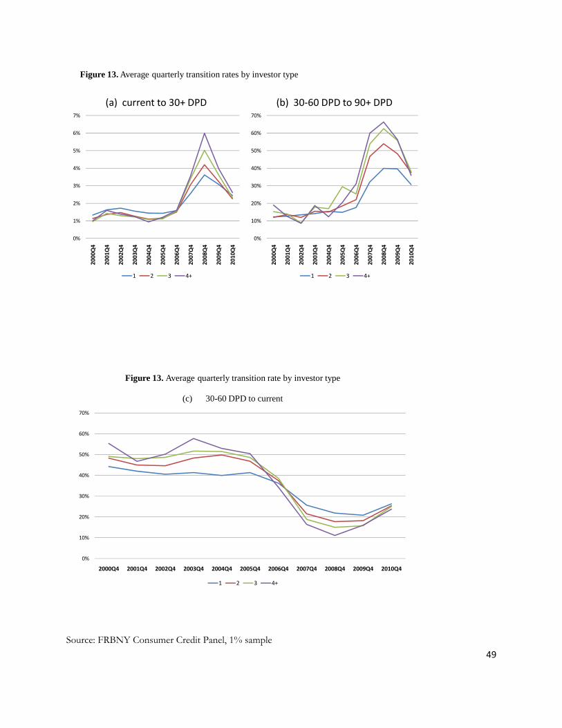
49 

 

 

 

Source: FRBNY Consumer Credit Panel, 1% sample 

Figure 13. Average quarterly transition rates by investor type

0%

1%

2%

3%

4%

5%

6%

7%

2000Q4

2001Q4

2002Q4

2003Q4

2004Q4

2005Q4

2006Q4

2007Q4

2008Q4

2009Q4

2010Q4

(a)  current to 30+ DPD

1 2 3 4+

0%

10%

20%

30%

40%

50%

60%

70%

2000Q4

2001Q4

2002Q4

2003Q4

2004Q4

2005Q4

2006Q4

2007Q4

2008Q4

2009Q4

2010Q4

(b)  30‐60 DPD to 90+ DPD

1 2 3 4+

0%

10%

20%

30%

40%

50%

60%

70%

2000Q4 2001Q4 2002Q4 2003Q4 2004Q4 2005Q4 2006Q4 2007Q4 2008Q4 2009Q4 2010Q4

Figure 13. Average quarterly transition rate by investor type

(c) 30-60 DPD to current

1 2 3 4+

 

50 

 

 

Source: FRBNY Consumer Credit Panel, 1% sample

Figure 14. Investor effect on quarterly flow into 90+ delinquency

‐0.30%

‐0.20%

‐0.10%

0.00%

0.10%

0.20%

0.30%

0.40%

0.50%

cross‐sectional investor definition

yearyear and stateyear, state and vintageyear, state, vintage, and loan type

panel investor definition

year

year and state

year, state and vintage

year, state, vintage, and loan type