real options in petroleum: geometric brownian motion and ...mikael.pelet.free.fr/20030912-real...

$: Real Options in Petroleum: Geometric Brownian Motion and ...mikael.pelet.free.fr/20030912-Real Options in petroleum_MRJ vs GBM... · This option is a so-called \Real Option" and its$
Real Options in Petroleum:

Geometric Brownian Motion and

Mean-Reversion with Jumps

Mikael PELETNew College

Oxford University

A dissertation submitted in partial fulfillment of the requirements for the degree ofMSc. in Mathematical Modelling and Scientific Computing

September 12, 2003

Acknowledgements

Special thanks to my supervisor, Dr William Shaw and to Dr Jeff Dewynne, for playing amajor role in directing me through this dissertation. I would like to extend my gratitudeto Dr Andy Wathen, my College advisor, for his sound advice and to Dr Hilary Ockendonfor her continuous support. And a very special thanks to the EPSRC for allowing meto come and study this year at Oxford University.

I, Mikael Pelet, hereby declare that the content of this dissertation is entirely myown work (except where otherwise indicated), that it has not been submitted for adegree of any other university, and that all the assistance I have received has been fullyacknowledged.

Mikael PeletNew CollegeSeptember 12, 2003

1

Abstract

The traditional Real Options model, developed by Paddock, Siegel & Smith, assumesthe underlying stochastic variable to follow a Geometric Brownian process. In the caseof a commodity, however, basic microeconomics and politics dictates that the price ofthe commodity ought to be related to its long-run marginal production cost, which isnot the case with a Geometric Brownian process. This process, moreover, does nottake into consideration the possible arrival of abnormal information, likely to generatediscrete stochastic shocks.

By not modelling accurately the underlying’s price in the case of a commodity, theGeometric Brownian Motion may lead to great errors in estimating the value of anundeveloped petroleum reserve and in finding the optimal investment strategy in thereserve. In this dissertation, I first developed a numerical scheme for the GeometricBrownian Motion model. Then I built an underlying model that presented a bettereconomic logic for petroleum prices, i.e. a model using Mean-Reversion with Jumps. Iafterwards implemented a numerical scheme for this model and did a sensitivity analysisof the model parameters. I finally performed a comparison between the two models.

Contents

1 Introduction 5

1.1 Real Options Theory . . . . . . . . . . . . . . . . . . . . . . . . . . . . . 5

1.2 Modelling Oil Prices . . . . . . . . . . . . . . . . . . . . . . . . . . . . . 5

1.3 Outline of the Dissertation . . . . . . . . . . . . . . . . . . . . . . . . . . 8

2 The Real Options Approach of Investment under Uncertainty 9

2.1 Generalities on Solving Real Option Problems . . . . . . . . . . . . . . . 9

2.1.1 Dynamic Programming . . . . . . . . . . . . . . . . . . . . . . . 10

2.1.2 Contingent Claims Analysis . . . . . . . . . . . . . . . . . . . . . 10

2.2 The Value of a Developed Reserve . . . . . . . . . . . . . . . . . . . . . 10

3 Model Using Geometric Brownian Motion 13

3.1 The Value of an Undeveloped Reserve and the Optimal Development Rule 13

3.2 Solving the Equation . . . . . . . . . . . . . . . . . . . . . . . . . . . . . 16

3.2.1 Finite Difference Method . . . . . . . . . . . . . . . . . . . . . . 16

3.2.2 At the Limits . . . . . . . . . . . . . . . . . . . . . . . . . . . . . 17

3.2.3 Projected Gauss-Seidel Solution Scheme . . . . . . . . . . . . . . 18

3.3 Precision of the Scheme . . . . . . . . . . . . . . . . . . . . . . . . . . . 19

3.4 Influence of the Numerical Scheme Parameters . . . . . . . . . . . . . . 20

4 Model Using Mean Reversion with Jumps 22

4.1 Stochastic Process . . . . . . . . . . . . . . . . . . . . . . . . . . . . . . 22

4.2 Optimization Problem . . . . . . . . . . . . . . . . . . . . . . . . . . . . 25

4.3 Explicit Finite Difference Method . . . . . . . . . . . . . . . . . . . . . . 27

4.4 Discretization of the Jump Term . . . . . . . . . . . . . . . . . . . . . . 28

4.5 Stability of the Explicit FDM, Computation and Comments . . . . . . . 29

4.6 Parameter Estimation . . . . . . . . . . . . . . . . . . . . . . . . . . . . 30

1

4.7 Influence of the Numerical Scheme Parameters . . . . . . . . . . . . . . 33

5 Models Results and Comparison 35

5.1 Traditional Model . . . . . . . . . . . . . . . . . . . . . . . . . . . . . . 35

5.1.1 Influence of the GBM Model Parameters . . . . . . . . . . . . . . 35

5.1.2 Comparison with other Results . . . . . . . . . . . . . . . . . . . 37

5.1.3 How to Use the Results . . . . . . . . . . . . . . . . . . . . . . . 38

5.2 Mean-Reversion with Jumps Model . . . . . . . . . . . . . . . . . . . . . 39

5.2.1 General Shape of the Solution . . . . . . . . . . . . . . . . . . . . 39

5.2.2 Influence of the MRJ Model Parameters . . . . . . . . . . . . . . 39

5.2.3 Evolution of the Option Value over Time . . . . . . . . . . . . . 44

5.3 Comparison between the Two Models . . . . . . . . . . . . . . . . . . . 44

6 Conclusion 46

6.1 Summary . . . . . . . . . . . . . . . . . . . . . . . . . . . . . . . . . . . 46

6.2 Possible Improvements . . . . . . . . . . . . . . . . . . . . . . . . . . . . 47

A Calculation details 49

A.1 Autoregressive Process . . . . . . . . . . . . . . . . . . . . . . . . . . . . 49

B MATLAB Code 51

B.1 American Option Pricing . . . . . . . . . . . . . . . . . . . . . . . . . . 51

B.2 Mean-Reversion with Jumps . . . . . . . . . . . . . . . . . . . . . . . . . 54

2

List of Figures

1.1 Yearly oil price history from 1900 to 1957 . . . . . . . . . . . . . . . . . 6

1.2 Monthly oil price history from 1957 to 2003 . . . . . . . . . . . . . . . . 7

3.1 Grid disposition . . . . . . . . . . . . . . . . . . . . . . . . . . . . . . . . 18

3.2 Option value and corresponding ∆ . . . . . . . . . . . . . . . . . . . . . 19

3.3 Comparison with Black-Scholes answers for the option value . . . . . . . 20

3.4 Comparison with Black-Scholes answers for ∆ . . . . . . . . . . . . . . . 20

3.5 What if Pm changes . . . . . . . . . . . . . . . . . . . . . . . . . . . . . 21

3.6 What if the grid gets finer . . . . . . . . . . . . . . . . . . . . . . . . . . 21

3.7 A very precise result . . . . . . . . . . . . . . . . . . . . . . . . . . . . . 21

4.1 Real world jumps distribution . . . . . . . . . . . . . . . . . . . . . . . . 23

4.2 Random jumps distribution . . . . . . . . . . . . . . . . . . . . . . . . . 25

4.3 Discretization of the jump . . . . . . . . . . . . . . . . . . . . . . . . . . 29

4.4 Influence of Pm and dΦ on the MRJ model . . . . . . . . . . . . . . . . 34

4.5 Influence of the grid size on the MRJ model . . . . . . . . . . . . . . . . 34

5.1 Option price and threshold evolution when r changes . . . . . . . . . . . 36

5.2 Option price and threshold evolution when δ changes . . . . . . . . . . . 36

5.3 Option price and threshold evolution when σ changes . . . . . . . . . . 36

5.4 Option price and threshold evolution when q changes . . . . . . . . . . . 37

5.5 Critical value for development of oil reserves . . . . . . . . . . . . . . . . 37

5.6 MRJ Option Value . . . . . . . . . . . . . . . . . . . . . . . . . . . . . . 39

5.7 Influence of the volatility on the MRJ model . . . . . . . . . . . . . . . 41

5.8 Effect of volatility on the MRJ threshold . . . . . . . . . . . . . . . . . . 41

5.9 Influence of the mean-reversion speed on the MRJ model . . . . . . . . 41

5.10 Influence of the jump arrival frequency on the MRJ model . . . . . . . . 42

5.11 Threshold function of the jump arrival frequency . . . . . . . . . . . . . 42

3

5.12 Influence of the long-run average oil price on the MRJ model . . . . . . 42

5.13 Influence of the exogenous discount rate on the MRJ model . . . . . . . 43

5.14 Influence of the jump-up average and standard deviation on the MRJ model 43

5.15 Influence of the economic quality of the reserve on the MRJ model . . . 43

5.16 Threshold comparison . . . . . . . . . . . . . . . . . . . . . . . . . . . . 45

6.1 Probability density function of Φ . . . . . . . . . . . . . . . . . . . . . . 47

4

Chapter 1

Introduction

1.1 Real Options Theory

Financial derivatives have known a great success in the 1980s. This lead to the de-velopment of the theory of Real Options (or theory of irreversible investment underuncertainty). Indeed, the main idea underlying Real Options is that financial deriva-tives, which are traded on many markets at extremely high volumes, can also be usedto model micro-economic decisions.

A simple analogy can illustrate this point: take for instance a company that wishesto invest in a project. Imagine that this company possesses the option to wait for betterconditions to implement this investment. This option is in fact very much like a financialderivative, and its underlying consists of the economic variables that will condition thefuture value of the project (such as the market share, the value of the products sold orbought or the intensity of demand). This option is a so-called “Real Option” and itsvaluation is similar to that of financial derivatives.

The Real Options approach appears to be much better than the traditional methodof Net Present Value, thereafter denoted NPV, in order to decide whether to investor not. In the NPV approach, expected future cash flows to leaseholders are determined,discounted to the present and summed to yield the lease value. To determine expectedcash flows and proper discount rates, it is first necessary to specify a statistical distri-bution (not necessarily independent) for exploration costs, quantities of hydrocarbonreserves, development costs, hydrocarbon prices and operating costs. But by boilingdown all the possibilities for the future into a single scenario, NPV does not account forthe ability of executives to react to new circumstances - for instance, spend a little upfront, see how things develop, then either cancel or go full speed ahead.

1.2 Modelling Oil Prices

The most common Real Options model was developed by Paddock, Siegel and Smith[18] between 1983 and 1988. It models the underlying’s price as a Geometric Brownian

5

Motion.

If one considers commodities, however, this model may not be accurate enough sincethe natural choice for modelling commodities seems to be mean-reversion processes. In-deed, basic microeconomics theory tells us that the price of a commodity ought to betied to its long-run marginal production cost, which varies largely across the countriesmainly because of the geologic features. Generally, marginal interaction between pro-duction and demand, between depletion and new reserve discoveries leads to smoothprice changes. In the case of oil, as it is a cartelized commodity, the situation is a littlebit more complicated. Indeed, the oil price is also tied to the long-run profit-maximizingprice sought by cartel managers. The role of OPEC furthermore remains very importantin the production game of the petroleum industry as most of the lower cost countriesbelong or are influenced by the OPEC cartel. For instance, the large rise in oil pricesin February-April 1999 (Figure 1.2) is mainly due to the articulation power of OPEC inreducing the production.

In Figure 1.1 and 1.2, one can see the evolution of oil prices over the last century.The prices for these figures as well as throughout this dissertation are real prices, theyhave been compounded with inflation and are expressed in terms of 04/2003 US$. Forthe purpose of this dissertation, Figure 1.2 is more relevant, as the time scale is betteradapted to the Real Options problem.

Figure 1.1: Yearly Prices of Brent and Similar Oils from 1900 to 1957

6

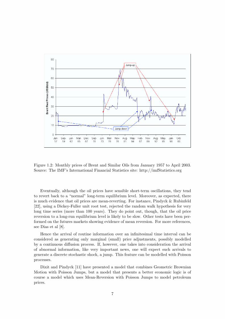
Figure 1.2: Monthly prices of Brent and Similar Oils from January 1957 to April 2003.Source: The IMF’s International Financial Statistics site: http://imfStatistics.org

Eventually, although the oil prices have sensible short-term oscillations, they tendto revert back to a “normal” long-term equilibrium level. Moreover, as expected, thereis much evidence that oil prices are mean-reverting. For instance, Pindyck & Rubinfeld[22], using a Dickey-Fuller unit root test, rejected the random walk hypothesis for verylong time series (more than 100 years). They do point out, though, that the oil pricereversion to a long-run equilibrium level is likely to be slow. Other tests have been per-formed on the futures markets showing evidence of mean reversion. For more references,see Dias et al [8].

Hence the arrival of routine information over an infinitesimal time interval can beconsidered as generating only marginal (small) price adjustments, possibly modelledby a continuous diffusion process. If, however, one takes into consideration the arrivalof abnormal information, like very important news, one will expect such arrivals togenerate a discrete stochastic shock, a jump. This feature can be modelled with Poissonprocesses.

Dixit and Pindyck [11] have presented a model that combines Geometric BrownianMotion with Poisson Jumps, but a model that presents a better economic logic is ofcourse a model which uses Mean-Reversion with Poisson Jumps to model petroleumprices.

7

1.3 Outline of the Dissertation

In the second chapter, I shortly introduce the context we place ourselves in, as wellas the two procedures for solving Real Options Problems: Dynamic Programming andContingent Claims Analysis. I then present the approach developed by Paddock, Siegel& Smith [18] to appraise developed reserves.

In the third chapter, I develop the traditional Geometric Brownian Motion model,thereafter denoted by GBM. I show its underlying theory and its numerical implemen-tation. I also discuss the precision of the latter.

In the fourth chapter, I develop the more complex Mean-Reversion with Jumpsmodel, thereafter denoted by MRJ. I derive a new differential equation related to thisnew approach of modelling the underlying and I estimate the parameters of this model.

In the fifth chapter, I first discuss the influence of the various model parameters onthe option price and threshold of the two models. I then compare the two models.

The sixth chapter presents a summary of the results as well as some possible waysin which the MRJ model could be improved.

In the Appendixes, details about some calculations are to be found, along with theMatlab code that was used to numerically implement the two models.

8

Chapter 2

The Real Options Approach ofInvestment under Uncertainty

The valuation of offshore leases is an important issue in itself. Firms perform valuationsas inputs to their bidding decisions. The government uses valuation to establish pre-sale reservation prices and to study the effect of policy changes on revenues it expectsto receive from lease sales. Because the bidding process involves billions of dollars, itis important to obtain accurate valuations. Interestingly, government valuations havetended to underestimate industry bids.

Embedded in any approach to valuing petroleum leases is a rule specifying whenand if a firm should explore and develop a particular leased property (i.e. exercise itsoption). The valuation and exploitation of an offshore oil tract can be viewed as partof a multistage investment problem. The first stage involves exploration - seismic testsand drilling to find out how much oil is present and the cost of extracting it. Thesecond stage (which would only occur if the exploration results are favorable) involvesdevelopment - the installation of the platforms and production wells that are needed toextract the oil. The last stage involves the extraction of the oil over a period of years.

The development expenditures convert undeveloped reserves into developed reserves.It is also important to bear in mind that the government subjects the leaseholder torelinquishment requirements that dictate how long a company can wait before beginningexploration and development.

Consider an oilfield discovered in the concession area, and suppose that the oilfield isdelineated (small geological uncertainty), so that is not optimal to continue the appraisalphase. The focus of the Real Option models is the development decision. The modelidentifies the optimal investment strategy and the oilfield value.

2.1 Generalities on Solving Real Option Problems

I now place myself in the case of the investment decision of a firm in a stochasticenvironment. At any time t the firm can invest in a project yielding an operating

9

profit that depends on a decision variable P (here the market price of oil) ruled by aparticular stochastic process.

In the literature, real options models are developed through two techniques closelyrelated to each other: dynamic programming and contingent claims analysis. Thesetechniques essentially differ about the assumptions they involve concerning investors,the financial markets and the discount rates used by investors. Due to these differences,the results they yield are similar although not identical.

One common characteristic of these models is the implicit assumption that actionsare taken instantaneously: the project is started as soon as the investor has decidedto invest. Using the stationary property and the Markovian property of the cash flowsgenerated by the project, traditional real options models consider that the investmentstarts as soon as the decision variable P hits some constant optimal level (see [11]).

2.1.1 Dynamic Programming

The first valuation method used in the real options literature amounts to finding theoptimization program of an investor through dynamic programming arguments. Thisinvestor is generally risk neutral and has rational expectations. He maximizes the presentvalue of the cash flow generated by the investment through an appropriate timing of theinvestment decision.

2.1.2 Contingent Claims Analysis

The other valuation method relies on an analogy between real and financial investmentdecisions. The firm has an option to invest in a project and the value of this option canbe found by the usual contingent claim valuation framework. The main assumption ofthis framework is that capital markets must be complete: there must exist an asset or adynamic portfolio of assets spanning the stochastic changes in the project value functionF (P, t).

2.2 The Value of a Developed Reserve

I denote here the quantity of barrels of oil in the ground (the volume of thepetroleum reserve) by B and the market value of one barrel from the reserve byV . I make the common assumption that this value is proportional to oil prices. Of course,this is a strong simplification and one could improve the model by taking a non-constantcoefficient of proportionality between V and P . I consider that the operating projectvalue W (P ), that is, the project value after the investment, can be conveniently givenby the following equation:

W (P ) = B · V (P ) = B · q · P. (2.1)

In my case V follows the same stochastic process as P . The proportion factor q describesthe economic quality of a developed reserve; a higher q implies higher market valuefor a barrel of oil in the ground (higher expected operational profit in present value fromthis underlying asset).

10

Now let R be the return over an instant of time to the owner of the developedreserve. The return will have two components: the flow of profit from production andthe capital gain on the remaining oil.

Due to the fall in pressure in the oilfield resulting from exploitation, the flow ofproduction from a developed reserve is best modelled as an exponential decline and afraction ω of the oil is produced each year:

dB = −ωBdt. (2.2)

Then, if I take Π as being the after-tax profit from producing and selling a barrelof oil, the return R can be expressed as

Rdt = ωBΠdt + d(BV )= ωBΠdt + BdV − ωV Bdt. (2.3)

I now have to assume that the rate of return on the developed reserve follows a givenstochastic process. I will place myself in the case of the GBM model and assume thatthe rate of return follows a Brownian motion process:

Rdt

BV= µdt + σdz, (2.4)

where the continuous time uncertainty is represented by the volatility σ and theWiener increment dz, and µ is the risk-adjusted expected rate of return re-quired by a competitive capital market.

Combining equations (2.3) and (2.4) gives the following equation for the dynamicsof V , the unit value of a developed reserve:

dV = (µ− δ)V dt + σV dz, (2.5)

where δ represents the payout rate from a unit of producing developed reserve:

δ = ωΠ− V

V. (2.6)

The economic quality of a developed reserve, linking the per-barrel value of a devel-oped reserve and the market price of oil is usually taken as being equal to one third.For the after-tax profit Π, I have to subtract the per-barrel costs, which are about 30percent of P , and the corporate tax rate, net of depreciation allowances, which is about34 percent. Hence, the after-tax profit on a barrel of oil is about 46 percent of the price.Finally, ω is usually around 12%, which leads to:

δ = 0.120.46P − 0.33P

0.33P≈ 0.05.

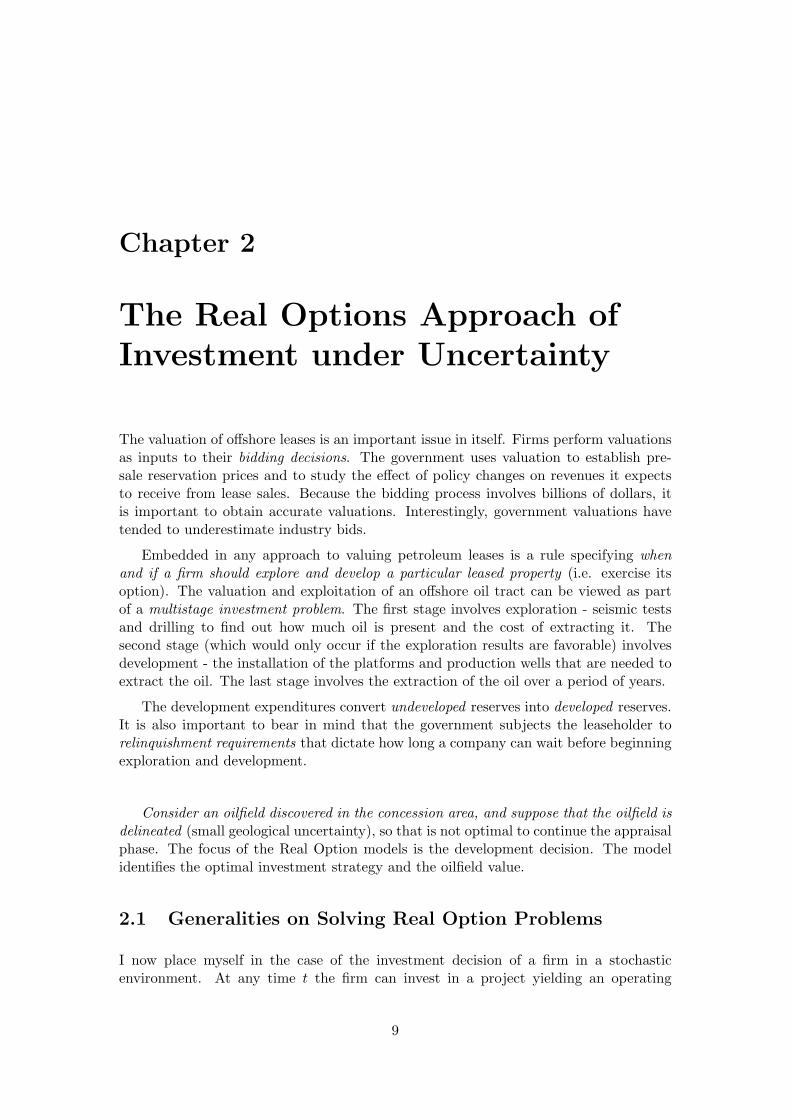
Thus holding a developed reserve is like holding a stock that has dividend yield of about5 percent. This is illustrated by the comparison presented in Table 2.1 between anAmerican Call Option and an Undeveloped Oil Reserve.

11

Call Option Undeveloped Reserve

Stock price Value of developed reserve

Exercise price Cost of development

Time to expiration Relinquishment requirement

Volatility of stock price Volatility of value of developedreserve

Dividend on stock Net production revenue fromdeveloped reserve less depletion

Table 2.1: Comparison between an American Call Option and an Undeveloped OilReserve

12

Chapter 3

Model Using GeometricBrownian Motion

3.1 The Value of an Undeveloped Reserve and the OptimalDevelopment Rule

Given equation (2.5) for the value of a developed reserve, I can now determine the valueof an undeveloped reserve as well as the optimal timing rule for its development. Sincethere are a variety of financial instruments that can be used to replicate fluctuations inthe price of oil (for example, futures contracts, forward contracts, and the shares of oilcompanies), spanning clearly holds and contingent claims methods can be used to valuean undeveloped reserve.

I am going to work with unitary values or per-barrel values. Of course, it is alsopossible to work with total values. NPV is used to express net present value per barrel:

NPV = V (P )−D = q · P −D, (3.1)

where D is the per-barrel cost of developing the reserve (that is, the “exerciseprice” of the option). Since I have chosen V (P ) = q · P where q is a constant, V and Pfollow the same stochastic process. So similarly to (2.5),

dP = (µ− δ)Pdt + σPdz. (3.2)

Now let F (P, t) denote the value of a one-barrel unit of undeveloped reserve.Using equation (2.5), I will construct a risk-free portfolio, determine its expected rateof return and equate that expected rate of return to the risk-free rate of interest.

I consider the following portfolio: hold the option to invest (worth F (P, t)), and goshort n units of the project. One important issue is whether you can actually hedgethe risk in any project related to the oil industry, and if so, how? That is, how inpractice do I get short my n units of the project.

In general by investing in the petroleum industry, what I have to fear is that afterinvesting, the oil price decreases too much for my investment to be profitable. Say for

13

instance that I want to buy a futures contract on oil with a 10 years expiration date.Indeed, if I sell in 10 years future time, and that the price goes down, I have hedged myrisk. I still face two problems however:

• 10 years futures do not exist;

• If I have a problem in production, I am selling oil that I do not have.

To solve the first problem, what I do is use swaps: I get long in the short termand short in the long term. I buy tomorrow and sell in three months; in three monthsless one day, I repeat the operation. And with the rule of sums, (xi − xi+1) = first −last term, at last, I have bought tomorrow and sold in ten years (of course, there is adiscount factor e−rt intervening). This what I wanted: if the price of the barrel goesdown, my note compensates for the loss.

Now going back to the portfolio, its value is φ = F (P, t) − nV . This portfolio isdynamic in the sense that if P changes, n may change from one short interval of time tothe next. Hence, the composition of the portfolio will be changed. However, over eachshort interval of length dt, I hold n fixed.

An investor holding a long position in the project will demand the risk-adjusted rateof return µ ·V , which equals the capital gain α ·V (α = µ− δ) plus the dividend streamδ ·V . Since the short position includes n units of the project, it will require that n · δ ·Vdollars are paid out per time period; otherwise no rational investor will enter into thelong side of the transaction. Taking this payment into account, the total return fromholding the portfolio over a short time interval dt is

dF (P, t)− ndV

dPdP − δnV dt, (3.3)

withdV

dPdP = qdP. (3.4)

Since n is held fixed over this short interval, I do not have any terms involving dndP .

Now, Ito’s lemma applied to F (P, t) with P satisfying (3.2) gives

dF (P, t) = Ft(P, t)dt + FP (P, t)dP +12FPP (P, t)σ2P 2dt, (3.5)

as (dP )2 = σ2P 2dt, and the total return on the portfolio is

12FPP (P, t)σ2P 2dt + FP (P, t)dP + Ft(P, t)dt− nqdP − δnqPdt. (3.6)

In order to eliminate the drift in the real world, I take

n =1qFP (P, t), (3.7)

14

and the total return on the portfolio becomes

12σ2P 2FPP (P, t)dt + Ft(P, t)dt− δPFP (P, t)dt. (3.8)

If the return is risk-free, to avoid arbitrage possibilities, it must equal

rφdt = r[F (P, t)− FP (P, t)P ]dt, (3.9)

with r being the risk-free rate of return. Hence,

12σ2P 2FPP (P, t)dt + Ft(P, t)dt− δPFP (P, t)dt = r[F (P, t)− FP (P, t)P ]dt. (3.10)

Dividing by dt and rearranging gives the following differential equation that F (P, t)must satisfy:

12σ2P 2FPP + (r − δ)PFP − rF = −Ft. (3.11)

In addition, F (P, t) must satisfy the following boundary conditions that are typical forAmerican Call Options:

F (0, t) = 0, Absorbing barrier at P = 0 (3.12a)F (P, T ) = max[V (P )−D, 0], Expiration optimal condition (3.12b)F (P ∗, t) = V (P ∗)−D, Value matching at P ∗ (3.12c)

FP (P ∗, t) = VP (P ∗) = q. Smooth pasting condition (3.12d)

Equation (3.12a) is standard for call options and arises from the observation that ifP goes to zero, it will stay at zero (this is an implication of the stochastic process (3.2)for P ). Therefore the option to invest will be of no value if V = 0.

Let the instant t = T be the expiration of the concession option. At this timethe owner has two alternatives: to develop the field immediately or to give up theconcession, returning the tract to the National Agency. As the firm will choose themaximum between NPV and zero, condition (3.12b) just says that at expiration, theoption to develop will be exercised if V (P ) > D.

Conditions (3.12c) and (3.12d) address the early exercise feature of American optionsand come from consideration of optimal investment. The first one is the value-matchingcondition: upon investing, the firm receives a net payoff V (P ∗)−D, P ∗ being the priceat which it is optimal to invest.

The last equation (3.12d), known as “smooth pasting condition” (or “high-contact”),is equivalent to the optimum exercise condition, so alternatively the earlier exercise testcan be performed (the maximum between the lived option and the payoff V − D). IfF (P, t) was not continuous and smooth at the critical exercise point V (P ∗), one woulddo better by exercising at a different point.

15

3.2 Solving the Equation

3.2.1 Finite Difference Method

Equation 3.11 can be solved numerically by using a Crank-Nicholson1 Finite DifferenceMethod (thereafter denoted FDM).

The FDM consists in transforming the continuous domain of the P and t state vari-ables by a network or mesh of discrete points (grid). The Partial Differential Equation(thereafter denoted PDE) is converted into a set of finite difference equations, whichcan be solved by using the appropriate boundary conditions. The solution is reachedby proceeding backward through small intervals (∆P )s until finding the optimal pathP ∗(t) to every t. The Crank-Nicholson form of this method corresponds to a specificchoice of finite differences for this substitution.

I assume the following discretization:

F (P, t) ≡ F (i∆P, j∆t) ≡ Fi,j , (3.13)

where 0 ≤ i ≤ m and 0 ≤ j ≤ n with n = T∆t .

Now make the substitutions:

FPP ≈ 12

[Fi+1,j+1 − 2Fi,j+1 + Fi−1,j+1](∆P )2

+12

[Fi+1,j − 2Fi,j + Fi−1,j ](∆P )2

, (3.14a)

FP ≈ 12

[Fi+1,j+1 − Fi−1,j+1]2∆P

+12

[Fi+1,j − Fi−1,j ]2∆P

, (3.14b)

Ft ≈ [Fi,j+1 − Fi,j ]∆t

, (3.14c)

F = Fi,j . (3.14d)

I use the “forward-difference” for the t variable. Applying these approximations to thePDE and the boundary conditions, I get the following difference equation (assumingthat σ2

|r−δ| = O(1), which is consistent with the case I study. Otherwise I would haveused an upwind scheme):

12σ2(i∆P )2

[12

Fi+1,j+1 − 2Fi,j+1 + Fi−1,j+1

(∆P )2+

12

Fi+1,j − 2Fi,j + Fi−1,j

(∆P )2]

+ (r − δ)i∆P[12

Fi+1,j+1 − Fi−1,j+1

2∆P+

12

Fi+1,j − Fi−1,j

2∆P

]

− rFi,j +Fi,j+1 − Fi,j

∆t= 0,

1This is also spelt Nicolson. Apologies if I wrote it the wrong way round.

16

14σ2i2

[(Fi+1,j+1 − 2Fi,j+1 + Fi−1,j+1) + (Fi+1,j − 2Fi,j + Fi−1,j)

]

+14(r − δ)i

[(Fi+1,j+1 − Fi−1,j+1) + (Fi+1,j − Fi−1,j)

]

− rFi,j +Fi,j+1 − Fi,j

∆t= 0,

and finally,

AiFi−1,j + BiFi,j + CiFi+1,j = aiFi−1,j+1 + biFi,j+1 + ciFi+1,j+1, (3.15)

whereAi = 1

4

(− σ2i2 + (r − δ)i)∆t, (3.16a)

Bi = 1 +(

σ2i2

2 + r)∆t, (3.16b)

Ci = −14

(σ2i2 + (r − δ)i

)∆t, (3.16c)

ai = 14

(σ2i2 − (r − δ)i

)∆t, (3.16d)

bi = 1− σ2i2

2 ∆t, (3.16e)

ci = 14

(σ2i2 + (r − δ)i

)∆t. (3.16f)

3.2.2 At the Limits

We now study the boundary conditions of the FDM. Firstly, there is no problem fori = 0, as A0 = a0 = 0. Secondly, the upper space limit is approximated by Pm, suchthat Pm = m∆P and FPP → 0 as P

D → ∞. Hence, if FPP = 0, Fm+1 = 2Fm − Fm−1,which allows us to eliminate Fm+1 from equation 3.15.The new equation at the limit is thus:

AmFm−1,j + BmFm,j + Cm(2Fm,j − Fm−1,j−1) =amFm−1,j+1 + bmFm,j+1 + cm(2Fm,j+1 − Fm−1,j+1),

orAmFm−1,j + BmFm,j = amFm−1,j+1 + bmFm,j+1, (3.17)

with

Am = Am − Cm

Bm = Bm + 2Cm

am = am − cm

bm = bm + 2cm.

An alternate method would be to consider the new differential equation when S →∞,with FPP ∼ 0: {

Ft + (r − δ)PFP − rF = 0,F (P, T ) = qP −D,

17

which givesF ∼ qPe−δ(T−t) −De−r(T−t),

andFm,j = qPme−δ(T−j∆t) −De−r(T−j∆t).

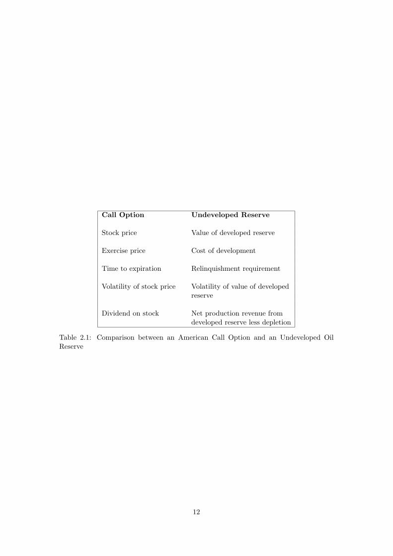
For the strike price, I choose to place D/q between two oil price steps, so that the oilprice derivatives of F remain bounded on the grid.

Figure 3.1: Grid disposition

3.2.3 Projected Gauss-Seidel Solution Scheme

Let us now define:Zi = aiFi−1,j+1 + biFi,j+1 + ciFi+1,j+1,

so that equation 3.15 becomes:

AiFi−1,j + BiFi,j + CiFi+1,j = Zi. (3.18)

Similarly to the method presented by Wilmott, Dewynne and Howison [25], I will usethe projected Gauss-Seidel method to solve the scheme.

The algorithm for finding the solution is iterative. At each time step, I start with aninitial guess U(0) = c, c being the final value obtained at the previous time step, andthe payoff function at the initial step. At each iteration, I create the vector

U(k+1) = (U (k+1)0,j , U

(k+1)1,j , . . . , U

(k+1)m,j ), (3.19)

from the current vectorU(k) = (U (k)

0,j , U(k)1,j , . . . , U

(k)m,j), (3.20)

using the following process: for each i = 0, 1, . . . , m, I sequentially calculate:

U(k+1)i,j =

1Bi

(Zi −AiU

(k+1)i−1,j − CiU

(k)i+1,j

), (3.21)

and compare it with the payoff w:

U(k+1)i,j = max(wi, U

(k+1)i,j ). (3.22)

This procedure implies the use of a loop. The stopping condition for this loop are either

||U(k+1) −U(k)|| < ε1 the change,

||Z−MU(k)|| < ε2 or the residual.

18

The residual, for an american option, is∑

Un>payoff

(Zi −AiU

(k)i−1,j −BiU

(k)i,j − CiU

(k)i+1,j

)2.

I then take U(k+1) as the solution, U(k)i,j = Fi,j+1, and reset the initial guess c = Fj+1.

3.3 Precision of the Scheme

For Matlab Code, see Appendix B.1.

I used the following procedure to evaluate the precision of the numerical scheme trougha graphical method. If there is no dividend (δ here) for the option I want to price, theprice of an American Call is the same as the price of an European Call. Hence, I candetermine the precision of my scheme by comparing the values I obtain with the exactvalues given by Black-Scholes. I will perform that verification on the option price, butalso on the first of the “Greeks”, ∆ = ∂F

∂P .

The shapes of the functions are as shown in Figure 3.2. The parameters for thisfigure are T = 10 years, r = 0.05, δ = 0, σ = 0.22, D = 5.25, Pm = 30, dP = 0.5,dt = 0.005, q=1/3 and the authorized variation in residual is 10−6. All the calculationspresented here have been preformed with the same parameters, unless otherwise stated.

05

1015

2025

30

0

2

4

6

8

100

1

2

3

4

5

6

7

Oil Prices (US$/bbl)Time (years)

Val

ue o

f the

con

cess

ion

(Opt

ion)

(US

$/bb

l)

(a) Option value over 10 years

05

1015

2025

30

0

2

4

6

8

100

0.05

0.1

0.15

0.2

0.25

0.3

0.35


Del

ta

(b) Value of ∆ over 10 years

Figure 3.2: Option value and corresponding ∆ obtained with the previous method

One can see in Figure 3.3 that the error over the whole price range is of order 10−3,i.e. 0.1%. The error in ∆ is of same order (Figure 3.4). The error tends to get biggerat the limits of the mesh. This is normal if one considers the relevant α = 1

2σ2P 2 ∆t(∆P )2

.This α is not constant over the grid and tends to get big at the upper P boundary.

Moreover, the error tends to fluctuate around the strike price. This is particularlyvisible when the exercise price is at a grid-point. This situation should be avoided asmuch as possible, as it leads to discontinuities in the derivatives of the option value.The best position for the strike price is right in the middle of two oil price grid-points,as I took it.

19

05

1015

2025

30

0

2

4

6

8

10−0.03

−0.025

−0.02

−0.015

−0.01

−0.005

0

0.005


Diff

eren

ce w

ith B

lack

−S

chol

es

(a) Difference between the Black-Scholes valuesand the calculated values

05

1015

2025

30

0

2

4

6

8

10−4

−3.5

−3

−2.5

−2

−1.5

−1

−0.5

0

0.5

x 10−3


Rel

ativ

e di

ffere

nce

with

Bla

ck−

Sch

oles

(b) Relative difference between the Black-Scholes values and the calculated values

Figure 3.3: Comparison between the Black-Scholes values and the option values obtainedwith the previous method

05

1015

2025

30

0

2

4

6

8

10−2.5

−2

−1.5

−1

−0.5

0

0.5

x 10−3


Diff

eren

ce w

ith B

lack

−S

chol

es D

elta

(a) Difference between the Black-Scholes ∆ val-ues and the calculated values

05

1015

2025

30

0

2

4

6

8

10−8

−6

−4

−2

0

2

x 10−3


Rel

ativ

e di

ffere

nce

with

Bla

ck−

Sch

oles

Del

ta

(b) Relative difference between the Black-Scholes ∆ values and the calculated values

Figure 3.4: Comparison between the Black-Scholes ∆ values and the ∆ values obtainedwith the previous method

3.4 Influence of the Numerical Scheme Parameters

The next question is: what happens to the error when the grid size, the oil price axistruncation value, or the allowed error in the residual change? In each of the follow-ing figures, all the parameters dP , Pm, dt, T , D and the authorized variation in theresidual remain the same, apart from the parameter mentioned in the caption of thecorresponding figure.

While increasing Pm can prove a good idea as it increases precision (Figure 3.5), onecan notice in Figure 3.6 that a finer grid does not necessarily lead to a better result.This is due to the presence of the term in σ, the second oil price derivative. The iterativesolver does not converge as well when one doubles the number of points, as the iterationmultiplies the error. The solution is to decrease the authorized variation in the residual.Eventually, good precision can be obtained by taking the parameters of Figure 3.7.

20

010

2030

4050

0

2

4

6

8

10−3

−2.5

−2

−1.5

−1

−0.5

0

0.5

1

x 10−3


Diff

eren

ce w

ith B

lack

−S

chol

es

(a) Evolution when Pm = 45

010

2030

4050

0

2

4

6

8

10−3

−2

−1

0

1

2

3

x 10−4


Rel

ativ

e di

ffere

nce

with

Bla

ck−

Sch

oles

(b) Relative evolution when Pm = 45

Figure 3.5: Evolution when Pm change

05

1015

2025

30

0

2

4

6

8

10−0.03

−0.025

−0.02

−0.015

−0.01

−0.005

0

0.005


Diff

eren

ce w

ith B

lack

−S

chol

es

(a) Evolution when dP=0.25 and dt=0.001

05

1015

2025

30

0

2

4

6

8

10−4

−3.5

−3

−2.5

−2

−1.5

−1

−0.5

0

0.5

x 10−3


Rel

ativ

e di

ffere

nce

with

Bla

ck−

Sch

oles

(b) Relative evolution when dP=0.25 anddt=0.001

Figure 3.6: Evolution when dP and dt change

010

2030

4050

60

0

2

4

6

8

10−20

−15

−10

−5

0

5

x 10−4


Diff

eren

ce w

ith B

lack

−S

chol

es

(a) Variation with Black-Scholes

010

2030

4050

60

0

2

4

6

8

10

−8

−6

−4

−2

0

2

4

x 10−5


Rel

ativ

e di

ffere

nce

with

Bla

ck−

Sch

oles

(b) Percentage variation

Figure 3.7: Difference with Black-Scholes when T = 10 years, D = 5.125, dP = 0.25,dt = 0.001, Pm = 60 and the authorized variation in residual is 10−20

21

Chapter 4

Model Using Mean Reversionwith Jumps

4.1 Stochastic Process

Again, let P be the spot price of a barrel of oil. As I said before, the prices most ofthe time change continuously as a mean-reverting process, but sometimes they changediscretely by jumps. In this way, the oil prices follow the stochastic differential equation(SDE):

dP

P=

[η(P − P )− λk

]dt + σdz + dq,

dq ={

0, with probability 1− λdt,Φ− 1, with probability λdt,

(4.1)

k = E(Φ− 1),

where E(Φ− 1) is the expected value of Φ− 1 with respect to the density of Φ.

Equation (4.1), which describes the rate of variation of oil prices (dP/P ), has threeterms on the right side.

• The first term is the mean-reverting drift : the petroleum price has a tendency togo back to the long-run equilibrium mean P with a reversion speed η. It iscompensated by λk for the Poisson jump expected value.

• The second term presents the continuous time uncertainty which is represented bythe volatility σ and the Wiener increment dz.

• The third term is the jump term, with the Poisson arrival parameter λ (thereis a probability λdt that a discrete jump will occur) and jump size Φ. The “minusone” appears as a matter of convention, as I define the probability density function(pdf) of Φ only over positive values and then translate the jump size.

One can determine the frequency and size of the jumps in the real world, if one sortsout the data on the oil price. Figure 4.1 shows the distribution of the jumps.

22

Figure 4.1: Real world jumps distribution: how many jumps occurred in 46 years andwhat was their size

Here is the code used to sort out the data:

jump=zeros(1,34);

for i=1:length(price)-1if price(i+1)/price(i)<0.1

jump(1)=jump(1)+1;elseif price(i+1)/price(i)>=0.1 & price(i+1)/price(i)<0.2

jump(2)=jump(2)+1;elseif price(i+1)/price(i)>=0.2 & price(i+1)/price(i)<0.3

...

...elseif price(i+1)/price(i)>=3.2 & price(i+1)/price(i)<3.3

jump(33)=jump(33)+1;elseif price(i+1)/price(i)>=3.3

jump(34)=jump(34)+1;end

end

I chose to consider any price change of over 20% in a month as a jump. As one cansee in Figure 4.1, in 46 years (I have taken only the period over which I had monthly data,i.e. between 1957 and 2003), 4 monthly jumps down and 6 jumps up have occurred. In

23

reality, however, some of these jumps were consecutive, therefore they are concatenatedand we are left with 3 jumps down and 4 jumps up. Of course, as the market tendsto absorb any jump in a period going from one to three month, I could have defined ajump as taking place over a period of more than one month.

Besides, as I only consider large jumps here, this model is not adapted for trading incommodities markets. It is clearly designed for projects of exploration and productionin petroleum.

The jumps-up quoted here have taken place during the Yom Kippur war and Arabianoil embargo in 1973/1974, during the Iran revolution and Iran/Iraq war in 1979/1980,during the Kuwait invasion by Iraq in 1990, and in 1999 as the OPEC and its alliescreated a supply shock. Jumps-down happened in 1957, in 1986 due to Saudi-Arabiaprice war and in 1991 after the Iraq defeat.

One notices that the jumps have random size. Hence I chose to model Φ as having aparticular probability distribution with mean k+1, represented by two truncated-normaldistributions: one normal distribution for the jump-up and one for the jump-down (seeFigure 4.2 below). In case of jump, this abnormal movement has the same chances ofbeing up or down. There is not enough data available in order to determine the exactparameters of both jumps. Hence, for reasons of simplicity, I defined the probabilitydensity function of Φ as:

pdf(Φ) =12

1σ1

√2π

e− 1

2(Φ−m1

σ1)2 +

12

1σ2

√2π

e− 1

2(Φ−m2

σ2)2

, (4.2)

with m1 = 12 , m2 = 2, σ1 = 1

8 , σ2 = 27 . Hence,

E(Φ) =m1 + m2

2, (4.3)

V (Φ) =σ2

1 + σ22

2+

(m1 + m2)2

4, (4.4)

and k = m1+m22 − 1.

Figure 4.2 shows that the exact size of each jump is uncertain. The same figureindicates that, in case of jump-up, the price is expected to double, whereas in case ofjump-down the price is expected to drop by half. I am interested in large jumps (as shownin the figure) but with low frequency (rare events).

This probability density function presents the drawback that the average jump sizeis bigger than 1. Thus over a long enough period, jumps will tend to increase the oilprice, although the probability of jump up is the same as the probability of jump down.Hence, one could improve the model by defining a different jump distribution whicheliminates this feature.

In addition, it is clear that Φ is not only positive, as the tails of the pdf are non-zeroat infinity. But as a simplification, the pdf in considered as being bounded at 0.

24

Figure 4.2: Random jumps distribution: probability density function of Φ

4.2 Optimization Problem

Again, the instant t = T is the expiration of the concession option. As with the GBMmodel, it is necessary to derive both the value of the concession (the value of the optionto invest) F (P, t), and the optimal decision rule (the threshold) P ∗(t ≤ T ). The decisionsare to develop, or to wait, or even to give up.

The solution procedure can be viewed as a maximization problem under uncertainty.I use the Bellman-dynamic programming framework (see Dixit & Pindyck, [11], chapter4) to solve the stochastic optimal control problem. I want to maximize the value of theconcession, the option F (P, t), seeking the instant when the price reaches a level P ∗ (thethreshold) in which one type of action is optimal.

Bellman’s Principle of Optimality states that an optimal policy has the propertythat, whatever the initial action, the remaining choices constitute an optimal policywith respect to the subproblem starting at the state that results from the initial actions.In short, that if at each step one chooses the optimal path, it leads to a globally optimalpath. This, of course, is not always true as shown by the Fermat principle.

Hence here, the Bellman equation, also called fundamental equation of optimality, is:

F (P, t) = maxP ∗(t)

{ [V (P )−D,E[F (P + dP, t + dt)e−ρdt]

], for all t < T

[V(P) - D, 0], for t = T

}, (4.5)

where ρ is an exogenous risk-adjusted discount rate and not necessarily a CapitalAsset Pricing Model (CAPM) risk-adjusted discount rate for the underlying asset whichwould require a complete market.

25

Indeed, CAPM looks at risk and rates of return and compares them to the overallmarket. If I use CAPM I have to assume that most investors want to avoid risk (riskaverse), and those who do take risks, expect to be rewarded.

µ = r + (rmarket − r)βxm, (4.6)

where µ is the risk-adjusted discount rate, r is the risk-free discount rate, rmarket is themarket discount rate and βxm is the coefficient of correlation between returns on theparticular asset x and the whole market portfolio m.

In case of incomplete markets, the risk-adjusted discount rate can be determined :

1. by “market-estimate”;

2. by choosing a risk-premium (hence getting the discount rate), specifying a utilityfunction for the investor;

3. by simply choosing an arbitrary exogenous value.

If I consider here the jump-risk as being systematic (correlated with the market portfo-lio), it is not possible to build a riskless portfolio. The market is not complete for thismodel with non-diversified jump risk, and one simply chooses an exogenous discountrate.

Using the Bellman equation and Ito’s Lemma, it is possible to build a partial differential-difference equation (PDE). I know:

dF =∂F

∂PdP +

12

∂2

∂P 2dP 2 +

∂F

∂tdt,

and dP 2 =(η(P − P )− λk

)2P 2dt2 + σ2P 2dz2 + P 2dq2

+ . . . dt · dz + . . . dt · dq + . . . dz · dq.

One knows that according to the definition of a Wiener process, E(dz) = 0 and E(dz2) =dt. One can also neglect all the terms whose expected value will be smaller than dt, i.e.the terms in dq2, dt · dz, dt · dq, dz · dq.

Now from 4.5 is a term in E[PFP dq] remaining. One knows that:

PFP dq ={

0 with probability 1− λdt,(Φ− 1)PFP with probability λdt.

(4.7)

Hence,

E[PFP dq] =λdtE[FP (P, t)(PΦ− P )] (4.8)=λdtE[F (PΦ, t)− F (P, t)], (4.9)

26

and I get the following PDE:

12σ2P 2FPP +

{η(P −P )−λE[Φ− 1]

}PFP +Ft +λE

[F (PΦ, t)−F (P, t)

]= ρF, (4.10)

with the same boundary conditions as for the GBM model.

Equation (4.10) is a PDE of parabolic type and is solved using the numerical methodof finite differences in the explicit form (see Section (4.3)). The parameters estimationis discussed in Section (4.6).

4.3 Explicit Finite Difference Method

To solve (4.10) I use the finite difference method in the explicit form. Assuming thesame discretization as previously, the partial derivatives are here approximated by thedifferences:

FPP ≈ [Fi+1,j − 2Fi,j + Fi−1,j ]/(∆P )2, (4.11a)

FP ≈ [Fi+1,j − Fi−1,j ]/2∆P, (4.11b)

Ft ≈ [Fi,j − Fi,j−1]/∆t. (4.11c)

I use the “central-difference” approximation for the P variable and the “backward-difference” for the t variable. Applying these approximations to the PDE and theboundary conditions, I get the following difference equation:

12σ2(i∆P )2

Fi+1,j − 2Fi,j + Fi−1,j

(∆P )2

+{

η(P − (i∆P )

)− λk

}(i∆P )

Fi+1,j − Fi−1,j

2∆P

+Fi,j − Fi,j−1

∆t+ λE

[FiΦ,j − Fi,j

]= ρFi,j−1,

and since E[FiΦ,j − Fi,j

]= E

[FiΦ,j

]− Fi,j , I get:

Fi,j−1 = p+Fi+1,j + p0Fi,j + p−Fi−1,j + pjumpE[Fi.Φ,j

], (4.12)

27

where

p+ =∆t

∆t.ρ + 1

[σ2i2

2+

i.(η.P )2

− i2.η.∆P

2− i.λ.k

2

], (4.13a)

p0 =∆t

∆t.ρ + 1

[1

∆t− σ2i2 − λ

], (4.13b)

p− =∆t

∆t.ρ + 1

[σ2i2

2− i.(η.P )

2+

i2.η.∆P

2+

i.λ.k

2

], (4.13c)

pjump =∆t

∆t.ρ + 1λ, (4.13d)

k = E[Φ− 1

]. (4.13e)

The boundary conditions are the same as for (3.12):

F0,j = 0, (4.14a)

Fi,n = max[qi∆P −D, 0], (4.14b)

Fi∗,j = qi∗∆P −D, (4.14c)

Fi∗+1,j − Fi∗−1,j = 2q∆P. (4.14d)

4.4 Discretization of the Jump Term

The last term in equation (4.12) represents the jump term contribution to the real optionvalue. Jumps can occur with probability pjump, and the expectation term is equivalentto a numerical integration of the options value over the new oil prices after the jumpoccurrence (i.∆P.Φ). To solve the numerical integration I perform a discretization overthe jump size distribution (Φ).

Besides, one can test that the probability of a jump tends toward one, by testing thejump with this code:

dPhi=1e-4; % Step size for discretisation of PDF of PhiL=3/dPhi % Number of steps

A_Phi=0;

for l = 1:LPhil = (l-1/2)*dPhi;prob = dPhi*pdf_phi(Phil);A_Phi=prob+A_Phi;

endA_Phi

28

Figure 4.3: The jump is discretized: the Φ axis is divided in L small partitions, withLdΦ = 3. The central value Φl−1/2 of each partition is associated to the correspondingprobability from the respective partition, i.e. p(Φl) = dΦf(Φl−1/2)

For dΦ=0.5, I obtain AΦ=0.71435, but for dΦ=0.1, AΦ=0.99988, as expected.

Now

E[FiΦ,j ] =L∑

l=1

p(Φl)F (iΦl). (4.15)

For any i in the interval 0 to m, iΦl is a real number. Hence, approximation or inter-polation methods have to be used to better approximate the new oil price after a jump(i.∆P.Φ) to some point (i.∆P ) inside the grid, while taking into account the truncationof the grid at Pm.

Essentially, the higher the number of the partitions the better the accuracy of the result.This numerical procedure can handle any kind of jump size distribution.

4.5 Stability of the Explicit FDM, Computation and Com-ments

In order to obtain stability, the discrete steps ∆P and ∆t must be chosen so that allthe coefficients (p+ , p0 , p−) from equation (4.12) are positive for any value inside thegrid. Therefore the stability of the explicit FDM determines the choice of ∆P and ∆t.

This condition is very demanding. The coefficient that usually poses problem is p0.

29

Small enough time steps have to be taken in comparison to the number of oil price stepsso that the first term in p0 is bigger than the second term. This implies the need for a finetime grid and a not so fine oil price grid, which would result in a very long computationtime and a poor precision in oil prices, especially penalizing for the threshold value.

It is furthermore not possible to calculate the option value for small volatility σwith this numerical scheme. Indeed, for the scheme to be consistent, one needs it to bediffusion dominated (i.e. 1

2σ2 À |η(P − P ) − λE[Φ − 1]|) so that the drift term in FP

does not take over the term in FPP . As for the GBM case, this feature is true here andif it was not, one could implement an upwind scheme, giving better stability but loosingprecision.

Finally, one could ask why I did not use the same numerical scheme as for the GBMmodel, i.e. Crank-Nicholson. This is because it would raise the issue of whether or notto work out the expectation term as an average over the two times and then workingwith non tri-diagonal matrices.

4.6 Parameter Estimation

Consider the following format for my model:

dP

P= η(P − P )dt + σdz + (Φ− 1)dq′ − λkdt (4.16)

where dq′ = 1 with probability λdt and zero otherwise. The last two terms are thecompensated-Poisson jump components (k = E[Φ− 1]).

Now, using Ito’s Lemma for the jump-diffusion case and the function x = log P (so that∂x/∂t = 0; ∂x/∂P = 1/P ; ∂2x/∂P 2 = −1/P 2) I get after some simplification:

dx = d(log P ) (4.17)

= ηP

log P

[log P

P

(P − σ2

2η

)− log P

]dt + σdz + (Φ− 1)dq′ − kλdt.

Comparing it with the simple equation

dx = η∗(x− x)dt + σ∗dz + jump-terms, (4.18)

I find the parameters:

η∗ = ηP

log P, (4.19)

x =log P

P

(P − σ2

2η

), (4.20)

σ∗ = σ. (4.21)

30

From these equations one gets the values of η, P and σ.

η = η∗log P

P, (4.22)

σ = σ∗, (4.23)

P =P

log Px +

σ2

2η. (4.24)

One could see here that there is a drawback with this method, as η and P depend on theoil price. Thus we must determine a representative oil price. I chose to use the mean ofthe price from 1957 to 2003.

Nonetheless, I am now looking for the mean-reverting parameters (x, η∗, σ∗).

For the estimation job, I put out the sample data referring to jumps, in order to estimateonly the mean-reverting parameters. I take the discrete time version of the equation4.18. As pointed out in Dixit & Pindyck [11], it is a first order autoregressive process.Specifically, equation (4.18) is the limiting case as ∆t → 0 of the following AutoregressiveProcess (see Appendix A.1):

xt − xt−1 = x(1− e−η∗) + (e−η∗ − 1)xt−1 + εt, (4.25)

where εt is normally distributed with mean zero and standard deviation σε, and

σ2ε =

σ∗2

2η∗(1− e−2η∗). (4.26)

Hence one can estimate the parameters by running the regression

xt − xt−1 = a + bxt−1 + εt (4.27)

and then calculating

x = −a

b, (4.28)

η∗ = − log(1 + b) and (4.29)

σ∗ = σε

√2 log(1 + b)(1 + b)2 − 1

. (4.30)

where σε is the standard error of the regression.

31

These operations are performed very easily in Matlab:

price; % price history excluding the jumpsx=log(price);

for i=1:length(price)-1delta_x(i)=x(i+1)-x(i);x_short(i)=x(i);

end

p = polyfit(x_short, delta_x, 1);%pop = polyval(p, x_short);%res = delta_x - pop;%

a = p(2) b = p(1)

disp(’mean of residual, should be zero =’);%disp(mean(res))sigma_eps = var(res)%eta_star = -log(1+b)%x_bar = -a/b%sigma_star = sigma_eps*sqrt(2*log(1+b)/((1+b)^2-1))%%%%%%%

eta = 12*eta_star * log(mean(price))/mean(price)%sigma = 12*sigma_star%P_bar = mean(price)*x_bar/log(mean(price)) + sigma^2/(2*eta)

I finally obtain the parameters I was looking for:

a 1 + b σ η P(monthly) (monthly) (% p.a.) (($/bbl)−1.year−1 ($/bbl)

0.033587 0.989109 18.11 0.031735 20.1189

Table 4.1: Estimated parameters for the Mean-Reverting model

I am now ready to implement the scheme into Matlab. For the calculations, I took intoconsideration the values generally adopted in the literature. For the volatility, Paddock,Siegel and Smith [18] mentioned that estimates based on data over the past 30 yearswould put σ at about 0.15, but that industry forecasts might be somewhat higher. Diasand Rocha [8] have made several more complex tests in order to estimate this parameter.

32

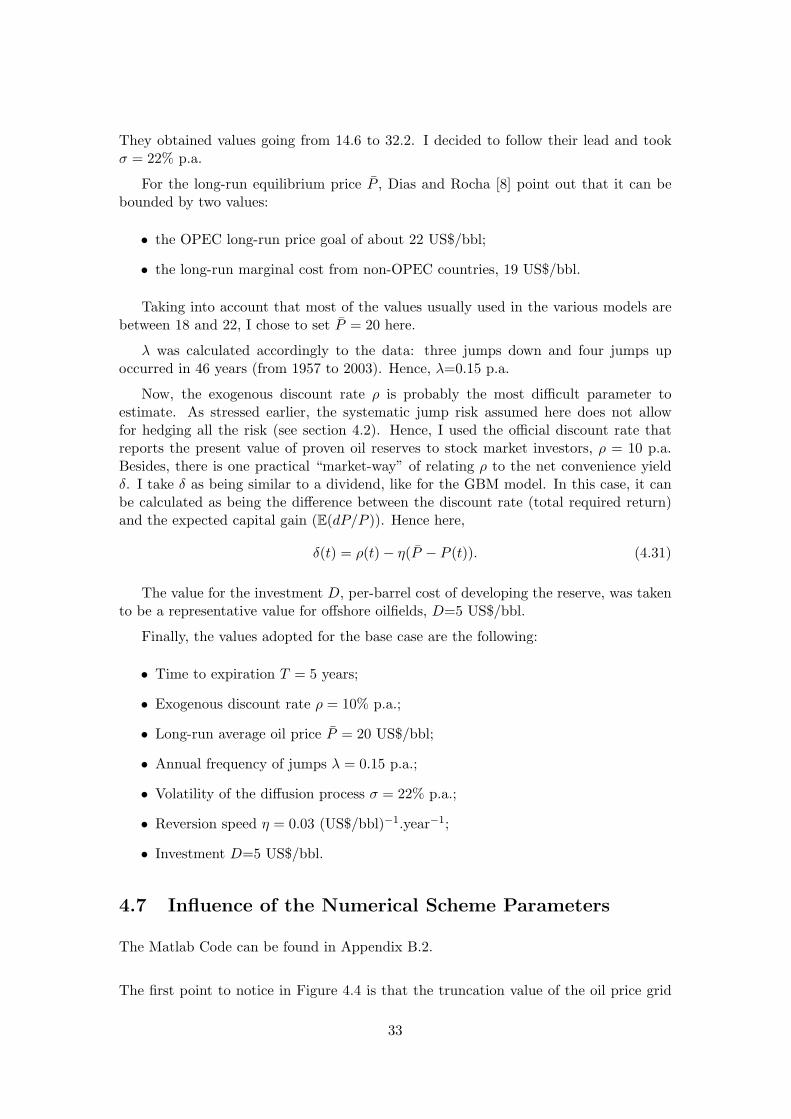
They obtained values going from 14.6 to 32.2. I decided to follow their lead and tookσ = 22% p.a.

For the long-run equilibrium price P , Dias and Rocha [8] point out that it can bebounded by two values:

• the OPEC long-run price goal of about 22 US$/bbl;

• the long-run marginal cost from non-OPEC countries, 19 US$/bbl.

Taking into account that most of the values usually used in the various models arebetween 18 and 22, I chose to set P = 20 here.

λ was calculated accordingly to the data: three jumps down and four jumps upoccurred in 46 years (from 1957 to 2003). Hence, λ=0.15 p.a.

Now, the exogenous discount rate ρ is probably the most difficult parameter toestimate. As stressed earlier, the systematic jump risk assumed here does not allowfor hedging all the risk (see section 4.2). Hence, I used the official discount rate thatreports the present value of proven oil reserves to stock market investors, ρ = 10 p.a.Besides, there is one practical “market-way” of relating ρ to the net convenience yieldδ. I take δ as being similar to a dividend, like for the GBM model. In this case, it canbe calculated as being the difference between the discount rate (total required return)and the expected capital gain (E(dP/P )). Hence here,

δ(t) = ρ(t)− η(P − P (t)). (4.31)

The value for the investment D, per-barrel cost of developing the reserve, was takento be a representative value for offshore oilfields, D=5 US$/bbl.

Finally, the values adopted for the base case are the following:

• Time to expiration T = 5 years;

• Exogenous discount rate ρ = 10% p.a.;

• Long-run average oil price P = 20 US$/bbl;

• Annual frequency of jumps λ = 0.15 p.a.;

• Volatility of the diffusion process σ = 22% p.a.;

• Reversion speed η = 0.03 (US$/bbl)−1.year−1;

• Investment D=5 US$/bbl.

4.7 Influence of the Numerical Scheme Parameters

The Matlab Code can be found in Appendix B.2.

The first point to notice in Figure 4.4 is that the truncation value of the oil price grid

33

Pm does not have as much effect on the option price as for the GBM model. This onlyholds as long as Pm remains above a certain value, which was found to be Pm = 40 inthis case.

The same remark can be made about the discretization of the jump. The step sizedΦ does not influence the result much, as long as it remains above a certain value. Thelimit in this case was found to be dΦ = 0.25.

In this section, the parameters have been taken as being dP = 0.5, dt = 5 · 10−4,Pm = 45, T = 5 years, D = 5.25, dΦ = 0.05 and q = 1/3 unless otherwise stated.

0 5 10 15 20 250

0.5

1

1.5

2

2.5

3

3.5

Oil Prices (US$/bbl)

Val

ue o

f the

con

cess

ion

(Opt

ion)

(US

$/bb

l)

Payoff

Reference Option Value

(a) Option price value when Pm = 90

0 0.5 1 1.5 2 2.5 3 3.5 4 4.5 515

16

17

18

19

20

21

22

Time (years)

Thr

esho

ld (

US

$/bb

l)

dΦ=0.1 dΦ=0.05

(b) Threshold evolution when dΦ=0.1

Figure 4.4: Influence of Pm and dΦ on the MRJ model

Though Pm and dΦ did not matter much, the grid size did, as shown in Figure4.5, where one can observe the effect of a change in dP over the option price and thethreshold.

0 5 10 15 20 25 30 35 40 450

1

2

3

4

5

6

7

8

9

10


Val

ue o

f the

con

cess

ion

(Opt

ion)

(US

$/bb

l)

dP=0.25

dP=0.5

(a) Option price evolution when dP = 0.25

0 0.5 1 1.5 2 2.5 3 3.5 4 4.5 515

16

17

18

19

20

21

22

Time (years)

Thr

esho

ld (

US

$/bb

l)

dP=0.5

dP=0.25

(b) Threshold evolution when dP=0.25

Figure 4.5: Influence of the grid size on the MRJ model

34

Chapter 5

Models Results and Comparison

5.1 Traditional Model

5.1.1 Influence of the GBM Model Parameters

What happens to the option price and the threshold when parameters such as r, δ, σ orq vary. The parameters for the numerical scheme were the same as for Figure 3.7. Thebase case to which all the values are compared is r = 5%, δ = 5%, σ = 22%, q = 1/3.

It is to be seen in Figure 5.1 that the interest rate increases both the option valueand the threshold. In order to understand why, imagine that I leave the money to pay aneventual option exercise in the bank. If the interest rate increases, I have less incentiveto exercise the option using that money; or in terms of present value, exercising theoption late instead of earlier is more attractive because the present value of the exerciseprice (the investment cost) is lower for the delay strategy.

The dividend (convenience) yield δ has an opposite effect compared with the interestrate, as shown on Figure 5.2. Dividend yield is like an opportunity cost of holding theunderlying asset. So, only the one who owns the underlying asset earns the flow ofbenefits associated with it (dividend yield). Higher δ means a lower value on waiting toinvest, therefore the threshold is lower and the live option has lower value.

Figure 5.3 shows that the volatility increases the option value and the threshold. Asuncertainty increases, delaying the investment proves to be a better strategy.S

Figure 5.4 shows that a greater economic quality of the reserve leads to greateroption value but decreases the threshold. All other parameters remaining identical, theproject has greater value and it is more interesting to invest if q is bigger.

Finally, the option price increases with r, σ and q and decreases with δ. Similarly,the threshold increases with r, σ but decreases this time with q and δ.

Moreover, as expected, higher time to expiration means higher option value. Butit is well known that there is an upper bound for this case. The perpetual Americanoption (with infinite time to expiration, as an option to develop a land) has a knownanalytic solution that is the upper bound for the option with the expiration time. SeeDixit & Pindyck [11].

35

0 10 20 30 40 50 600

5

10

15


Val

ue o

f the

con

cess

ion

(Opt

ion)

(US

$/bb

l)

r=10%

r=5%

(a) Option price evolution when r increases

0 1 2 3 4 5 6 7 8 9 1015

20

25

30

35

40

45

Time (years)

Thr

esho

ld (

US

$/bb

l)

r=10%

r=5%

(b) Threshold evolution when r increases

Figure 5.1: Option price and threshold evolution when r changes

0 5 10 15 20 25 300

0.5

1

1.5

2

2.5

3

3.5

4

4.5

5


Val

ue o

f the

con

cess

ion

(Opt

ion)

(US

$/bb

l)

Payoff

δ=5%

δ=10%

(a) Option price evolution when δ increases

0 1 2 3 4 5 6 7 8 9 1015

20

25

30

Time (years)

Thr

esho

ld (

US

$/bb

l)

δ=5%

δ=10%

(b) Threshold evolution when δ increases

Figure 5.2: Option price and threshold evolution when δ changes

0 10 20 30 40 50 600

5

10

15


Val

ue o

f the

con

cess

ion

(Opt

ion)

(US

$/bb

l)

σ=22%

σ=35%

(a) Option price evolution when σ increases

0 1 2 3 4 5 6 7 8 9 1015

20

25

30

35

40

45

Time (years)

Thr

esho

ld (

US

$/bb

l)

σ=35%

σ=22%

(b) Threshold evolution when σ increases

Figure 5.3: Option price and threshold evolution when σ changes

36

0 5 10 15 20 25 300

5

10

15


Val

ue o

f the

con

cess

ion

(Opt

ion)

(US

$/bb

l)

q=2/3 q=1/3

Payoff when q=2/3

Payoff when q=1/3

(a) Option price evolution when q increases

0 1 2 3 4 5 6 7 8 9 105

10

15

20

25

30

Time (years)

Thr

esho

ld (

US

$/bb

l)

q=1/3

q=2/3

(b) Threshold evolution when q increases

Figure 5.4: Option price and threshold evolution when q changes

5.1.2 Comparison with other Results

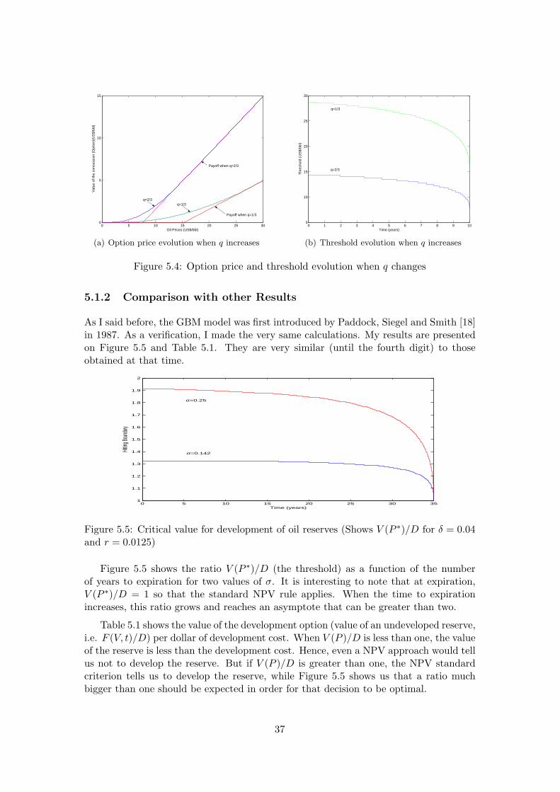
As I said before, the GBM model was first introduced by Paddock, Siegel and Smith [18]in 1987. As a verification, I made the very same calculations. My results are presentedon Figure 5.5 and Table 5.1. They are very similar (until the fourth digit) to thoseobtained at that time.

0 5 10 15 20 25 30 351

1.1

1.2

1.3

1.4

1.5

1.6

1.7

1.8

1.9

2

Time (years)

Hitting

Boun

dary

σ=0.25

σ=0.142

Figure 5.5: Critical value for development of oil reserves (Shows V (P ∗)/D for δ = 0.04and r = 0.0125)

Figure 5.5 shows the ratio V (P ∗)/D (the threshold) as a function of the numberof years to expiration for two values of σ. It is interesting to note that at expiration,V (P ∗)/D = 1 so that the standard NPV rule applies. When the time to expirationincreases, this ratio grows and reaches an asymptote that can be greater than two.

Table 5.1 shows the value of the development option (value of an undeveloped reserve,i.e. F (V, t)/D) per dollar of development cost. When V (P )/D is less than one, the valueof the reserve is less than the development cost. Hence, even a NPV approach would tellus not to develop the reserve. But if V (P )/D is greater than one, the NPV standardcriterion tells us to develop the reserve, while Figure 5.5 shows us that a ratio muchbigger than one should be expected in order for that decision to be optimal.

37

σ = 0.142 σ = 0.25V (P )/D T = 5 T = 10 T = 15 T = 5 T = 10

0.80 0.0181903 0.0286743 0.0338309 0.0750321 0.10575250.85 0.0277936 0.0396675 0.0452272 0.0929930 0.12508620.90 0.0405532 0.0533608 0.0591480 0.1131118 0.14612120.95 0.0569072 0.0700809 0.0758961 0.1353737 0.16884611.00 0.0772516 0.0901562 0.0957849 0.1597523 0.19324721.05 0.1019398 0.1139179 0.1191380 0.1862127 0.21930991.10 0.1312860 0.1417014 0.1462903 0.2147147 0.24701901.15 0.1655732 0.1738481 0.1775881 0.2452145 0.2763592

Table 5.1: Some option values for various parameters, calculated with the GBM model.Precision of 10−4.

5.1.3 How to Use the Results

It is now time to ask how does one use the results I have obtained, the value of theReal Option, to price an undeveloped reserve. For that purpose, I will use an exampleintroduced by paddock, Siegel and Smith [18] and used by Dixit and Pindyck [11].

Consider an undeveloped reserve which, if developed, is expected to yield 100 millionbarrels of oil and has a ten year relinquishment requirement. Let some assumptions bemade:

• the value of the developed reserve is $12 per barrel;

• the payout rate is 5% (just as a reminder, the payout rate is the net productionrevenues less depletion as a fraction of the reserve value);

• development takes three years;

• the present value of development cost is $11.79 per barrel.

Now the undeveloped reserve could be valued as follows:

• First I calculate the present value of the developed reserve, because of the threeyears development time. The correct discount rate is the difference between therisk-adjusted rate µ and the expected rate of growth of the reserve value (µ− δ),i.e. the payout rate δ. Hence, the present value of the developed reserve is V ′ =e−3∗0.05($12) = $10.32.

• Now the critical ratio (developed reserve value to the present value of the develop-ment cost) is V ′/D = $10.32/$11.79 ≈ 0.90. Being less than one, the developmentoption is out-of-the-money.

• It is time to use Table 5.1 to calculate the value of the undeveloped reserve.Assuming that σ is 0.142, the option value per dollar of development cost is 0.05336and the total development cost is ($11.79)(100 million)=$1179 million. Hence thetotal value of the undeveloped reserve is (0.05336)($1179 million) = $62.91 million.

38

Thus, the undeveloped reserve has a value of $63 million due to its option value,although it would not be profitable yet to develop it because of the oil prices. Imaginethough that the conditions on the oil market change in a way such that σ was 0.25. Thisnew perceived value of oil prices would increase the value of the undeveloped reserve to(0.14612)($1179 million) = $172.28 million!

5.2 Mean-Reversion with Jumps Model

5.2.1 General Shape of the Solution

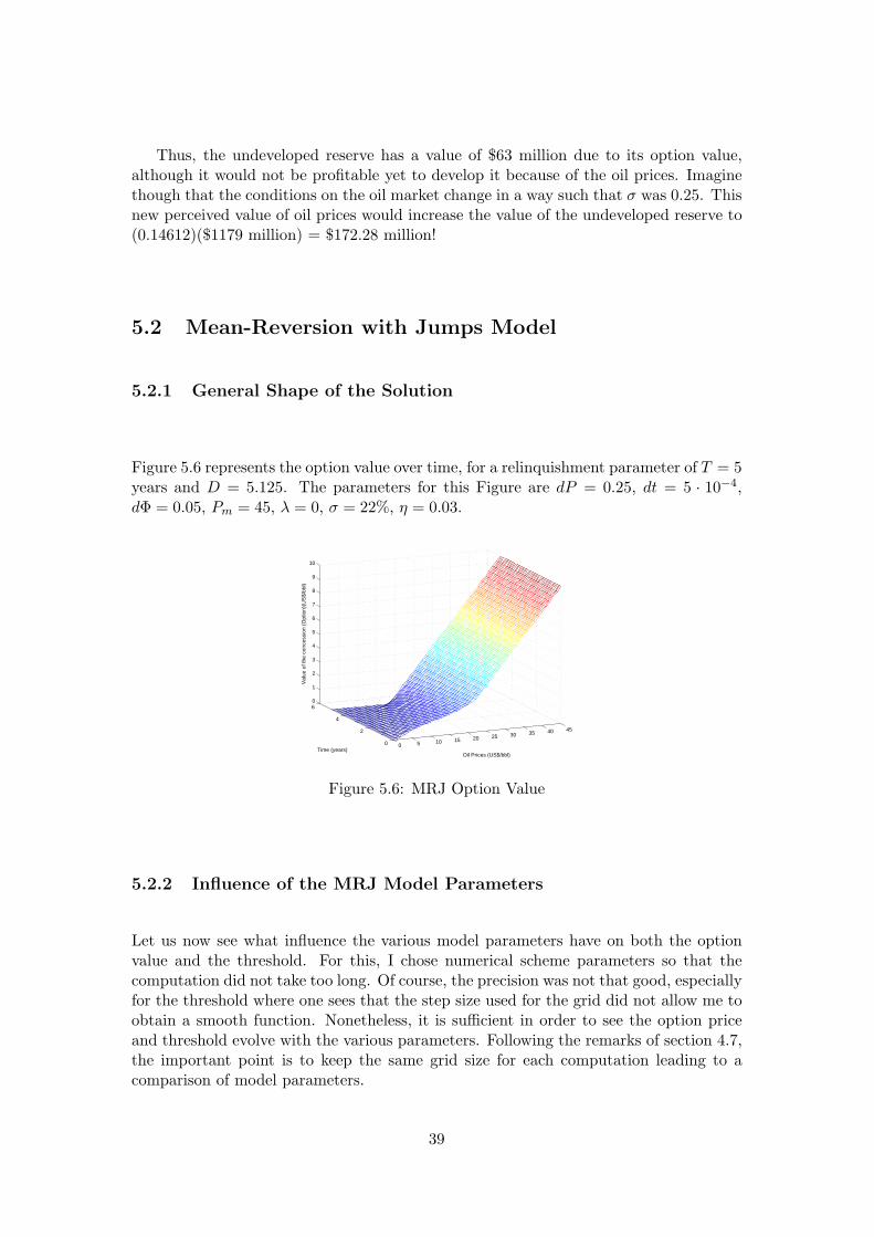
Figure 5.6 represents the option value over time, for a relinquishment parameter of T = 5years and D = 5.125. The parameters for this Figure are dP = 0.25, dt = 5 · 10−4,dΦ = 0.05, Pm = 45, λ = 0, σ = 22%, η = 0.03.

0 5 10 15 20 25 30 35 40 45

0

2

4

60

1

2

3

4

5

6

7

8

9

10


Val

ue o

f the

con

cess

ion

(Opt

ion)

(US

$/bb

l)

Figure 5.6: MRJ Option Value

5.2.2 Influence of the MRJ Model Parameters

Let us now see what influence the various model parameters have on both the optionvalue and the threshold. For this, I chose numerical scheme parameters so that thecomputation did not take too long. Of course, the precision was not that good, especiallyfor the threshold where one sees that the step size used for the grid did not allow me toobtain a smooth function. Nonetheless, it is sufficient in order to see the option priceand threshold evolve with the various parameters. Following the remarks of section 4.7,the important point is to keep the same grid size for each computation leading to acomparison of model parameters.

39

First, one can notice on Figures 5.7 and 5.8 that an increase in σ increases the optionvalue and the threshold. This result is similar to the one observed with the GBM model.

Figure 5.9 shows the influence of the mean-reversion speed η. An increase in ηincreases the option value as well as the threshold. Indeed, as the reversion speed isbigger, the oil price is more likely to remain around its long-run average price. Andas the strike price is below the long-run average oil price, the option value increases.Besides, when η is zero, the threshold is below the long-run average oil price, while it isabove the long-run average oil price for any other positive value of η.

Figures 5.10 and 5.11 show that the jump arrival factor λ tends to diminish boththe option value and the threshold. For higher jump frequency, the option price andthe threshold for immediate investment are lower. The economic explanation is that theprobability of a jump makes the investor more willing to invest. This is due to the biasin the probability density function I chose for the jump size, as the average jump size isgreater than one.

Figure 5.12 shows the influence of the long-run average oil price P over the optionprice and immediate investment threshold. One can notice that a lower P decreases theoption value as well as the threshold. Indeed, when the long-run average oil price iscloser to the strike price, the expected profit decreases. Furthermore, as the expectedoil price is lower, the threshold decreases as well.

The influence of the exogenous discount rate ρ is shown in Figure 5.13 and tends toreduce both the threshold and the option price. Indeed, given a fixed drift, the dividendor convenience yield δ has to adjust to ρ due to the relation 4.31. By increasing theconvenience yield, the value of waiting decreases as do the option value and the threshold.

In order to visualize the influence of the average jump-up size m2 (Figure 5.14), thejump distribution was modified so that the general shape remained the same. Only thejump-up was modified with an average at 3 instead of 2 and a standard deviation of2/3 instead of 2/7. I noticed then that the modification of the jump-up had a negativeinfluence over the option price and threshold. The explanation is the same as for theinfluence of the jump arrival rate. As the jump-up has a greater mean, the oil value isexpected to be bigger, hence decreasing the opportunity value of waiting.

The influence of the economic quality of the reserve shown on Figure 5.15 is thesame as for the GBM model.

Finally, as one can see on Table 5.3, the option value increases for higher volatility,for higher mean-reversion speed, for lower jump arrival rate, for higher long-run averageoil price, for lower exogenous discount rate, for lower average jump-up and for highereconomic quality of the reserve. The outcome is the same for the threshold, except forthe economic quality of the reserve, as the threshold decreases if q increases.

40

0 2 4 6 8 10 12 14 16 18 200

0.2

0.4

0.6

0.8

1

1.2

1.4

1.6

1.8


Val

ue o

f the

con

cess

ion

(Opt

ion)

(US

$/bb

l)

σ=15%

σ=10%

(a) Option price evolution when σ changes

0 0.5 1 1.5 2 2.5 3 3.5 4 4.5 517.5

18

18.5

19

19.5

20

Time (years)

Thr

esho

ld (

US

$/bb

l)

σ=15%

σ=10%

(b) Threshold evolution when σ changes

Figure 5.7: Influence of the volatility on the MRJ model

Figure 5.8: Effect of volatility on the MRJ threshold

0 2 4 6 8 10 12 14 16 18 20 220

0.5

1

1.5

2

2.5


Val

ue o

f the

con

cess

ion

(Opt

ion)

(US

$/bb

l)

η=0

η=0.03

(a) Option price evolution when η changes

0 0.5 1 1.5 2 2.5 3 3.5 4 4.5 515

16

17

18

19

20

21

Time (years)

Thr

esho

ld (

US

$/bb

l) η=0

η=0.03

(b) Threshold evolution when η changes

Figure 5.9: Influence of the mean-reversion speed on the MRJ model

41

0 5 10 15 200

0.5

1

1.5

2

2.5

3


Val

ue o

f the

con

cess

ion

(Opt

ion)

(US

$/bb

l)

λ=0%

λ=10%

λ=30%

(a) Option price evolution when λ changes

0 0.5 1 1.5 2 2.5 3 3.5 4 4.5 516

17

18

19

20

21

22

23

24

Time (years)

Thr

esho

ld (

US

$/bb

l)

λ=0%

λ=10%

λ=30%

(b) Threshold evolution when λ changes

Figure 5.10: Influence of the jump arrival frequency on the MRJ model

Figure 5.11: Threshold function of the jump arrival frequency for the base case

0 2 4 6 8 10 12 14 16 18 200

0.5

1

1.5


Val

ue o

f the

con

cess

ion

(Opt

ion)

(US

$/bb

l)

Mean−Reverting Oil Price is 15


(a) Option price evolution when P changes

0 0.5 1 1.5 2 2.5 3 3.5 4 4.5 515

16

17

18

19

20

21

22

Time (years)

Thr

esho

ld (

US

$/bb

l)



(b) Threshold evolution when P changes

Figure 5.12: Influence of the long-run average oil price on the MRJ model

42

0 2 4 6 8 10 12 14 16 18 200

0.5

1

1.5


Val

ue o

f the

con

cess

ion

(Opt

ion)

(US

$/bb

l)

ρ=15%

ρ=10%

(a) Option price evolution when ρ changes

0 0.5 1 1.5 2 2.5 3 3.5 4 4.5 515

16

17

18

19

20

21

22

Time (years)

Thr

esho

ld (

US

$/bb

l)

ρ=10%

ρ=15%

(b) Threshold evolution when ρ changes

Figure 5.13: Influence of the exogenous discount rate on the MRJ model

0 2 4 6 8 10 12 14 16 18 200

0.5

1

1.5


Val

ue o

f the

con

cess

ion

(Opt

ion)

(US

$/bb

l)

Average Jump− Up Size is 3


(a) Option price evolution when m2 and σ2

change

0 0.5 1 1.5 2 2.5 3 3.5 4 4.5 515

16

17

18

19

20

21

22

Time (years)

Thr

esho

ld (

US

$/bb

l)



(b) Threshold evolution when m2 and σ2 change

Figure 5.14: Influence of the jump-up average and standard deviation on the MRJ model

0 5 10 15 200

2

4

6

8

10

12


Val

ue o

f the

con

cess

ion

(Opt

ion)

(US

$/bb

l)

Payoff for q=2/3

Payoff for q=1/3 Option value for q=2/3

Option value for q=1/3

(a) Option price evolution when q change

0 0.5 1 1.5 2 2.5 3 3.5 4 4.5 56

8

10

12

14

16

18

20

22

Time (years)

Thr

esho

ld (

US

$/bb

l)

q=1/3

q=2/3

(b) Threshold evolution when q change

Figure 5.15: Influence of the economic quality of the reserve on the MRJ model

43

5.2.3 Evolution of the Option Value over Time

On Table 5.2, one can see the evolution of price with respect to the expiration date. Thepercentages shown are the variation between the value corresponding to one expirationdate to the next. One can notice that these variation are much more important out-of-the-money than in-the-money, and that the variations in the option price are much moreimportant than the variations in threshold. Indeed, if the expiration date goes from 2 to5 years, the option value out-of-the-money (P = 15) increases by 21%, the option valuein-the-money increases by 7.6%, whilst the threshold only increases by 2.4%. Hence,taken that the bid bonus is proportional to the option value, a later expiration dateimplies greater bid bonus without influencing the threshold value too much.

T (years) F (P = 15) % in F F (P = 18) % in F P ∗(0) % in P ∗

1 0.5114 - 1.0681 - 20 -2 0.6856 34.1% 1.1522 7.9% 20.5 2.5%3 0.7798 13.7% 1.2006 4.2% 20.75 1.2%4 0.8346 7.0% 1.2294 2.4% 21 1.2%5 0.8673 3.9% 1.2472 1.4% 21 0.0%

Table 5.2: Sensitivity of the option value and threshold with time to expiration for thebase case (Prices in $/bbl)

5.3 Comparison between the Two Models

One important issue for comparing the two models is to unify the variables. Let us taker = δ = 5% for the GBM model. The convenience yield δ is not a direct input parameterfor the MRJ model (it is implicit, endogenous of the model) and depends on the pricelevel. Hence, in order to compare the two models we need to choose the right price. Ithas been seen that δ = ρ − η(P − P ). Hence, by replacing by the latter values, I getP = 18.3.

Mean-Reversion + Jump Process: F (P = 18.3$/bbl, t = 0)Base No σ = 5% σ = 10% No σ = 23%,Case Jump Reversion λ = 0

(λ = 0) η = 0 and η = 01.3005 1.7743 1.0500 1.0804 1.0760 1.3425

Geometric Brownian Motion: F (P = 18.3$/bbl, t = 0)Base r = 10% r = 10%Case and and

r = δ = 5% δ = 5% δ = 10%1.4667 1.9084 1.3412

Table 5.3: Option value at P = 18.3 US $/bbl

44

As one can observe on Table 5.3, it is hard to make a comparison between the twomodels. Only for η = 0, implying ρ = δ, can one compare the case of GBM with r = δand MRJ with no reversion, no jump and the same volatility σ = 23%. As expected,the values are very close, as are the graphical solutions.

F (P = 12) F (P = D/q) F (P = 18) P ∗(t = 0) P ∗(t = 5)Jump-Reversion 0.5487 0.8427 1.2472 21 17.75

GBM 0.3689 0.8002 1.3959 26.8 15.6

Table 5.4: Comparing the two Real Options methods in the base case ($/bbl)

0 0.5 1 1.5 2 2.5 3 3.5 4 4.5 514

16

18

20

22

24

26

28

Time (years)

Thresh

old (U

S$/bb

l)

Threshold for GBM

Threshold for Jump−Diffusion

Figure 5.16: Threshold comparison: Jump Diffusion and Geometric Brownian Motion

Figure 5.16 and Table 5.4 show that in the base case, the MRJ threshold is smallerthan for GBM when the time to expiration is important. But the situation is reversedcloser to expiration. Furthermore, the option price is higher in the MRJ case than in theGBM case for an option out-of-the-money, but the situation is reversed for an option in-the-money, while the prices are similar at-the-money. Hence by using the GBM model,one would invest later, and in projects that may have been rejected if using MRJ closerto the deadline, and one may underestimate or overestimate the value of the projectdepending on the in-the-money/out-of-the-money situation.

45

Chapter 6

Conclusion

6.1 Summary

The advantage of jump-reversion process is that it better describes the reality of botheconomics (microeconomic logic) and statistical time-series (explaining the skewness,fatter tails, abnormal movements of oil prices). But there is a cost. The two problemswith jump-diffusion processes are the impossibility of building a riskless portfolio andthe difficulty of parameters estimation.

Nonetheless, the MRJ model is definitely more suitable to Real Options related tocommodities like oil. There can be huge differences between the option values yieldedby this model and the GBM model. It is of course difficult to compare the values of thetwo models, as they do not require the same assumptions nor use the same parameters.

One could however still observe that the behaviour of both models relative to theirparameters was as similar as it possibly could be. Indeed, both the GBM and MRJoption values increase with the volatility and the economic quality of the reserve, andtheir threshold increases with the volatility and decreases with the economic quality ofthe reserve. Besides, by noting the relation between the payout rate and the exogenousdiscount rate in the MRJ model, one notices that an increase in these parameters leadsto lower option values and threshold in both cases.

Some parameters in the MRJ model do not have equivalents in the GBM model andvice versa. For instance, the fact that the GBM option value and threshold increase withthe risk-free interest rate. Or the fact that the MRJ option value and threshold increasefor higher mean-reversion speed, for lower jump arrival rate, for higher long-run averageoil price and for lower average jump-up. But considering the case where the risk-freeinterest rate is equal to the payout rate and to the MRJ exogenous discount rate, andwhere there are no jumps and the mean-reversion speed is zero, the same solution isobtained.

In the base case I chose to study, using the GBM model would lead to later investing,and in projects that may have been rejected if using the MRJ model. Furthermore, thevalue of the project may be either underestimated or overestimated depending on thein-the-money/out-of-the-money situation.

Finally, the only drawback to be noticed by using the MRJ model with the scheme

46

that I implemented here is that the computation time is much longer than that for theGBM model with the corresponding numerical scheme.

6.2 Possible Improvements

The MRJ model presented here could be extended in several ways.

• One could implement a numerical scheme based on projected Gauss-Seidel, as usedwith the GBM model scheme. This was not done because of time constraints. Asa Crank-Nicholson Scheme has a faster convergence rate, this may decrease thecomputation time significantly.

• One could try a more complex probability density function for the jump size, al-though the available data for the oil price did not allow us to come up with a precisestatistical distribution. One could also try to use two uncorrelated distributionsfor jumps-up and jumps-down.

• Furthermore, I later discovered that another Mean-Reversion with Jumps SDE,could be used to better equilibrate the Jumps Process:

d(logP ) = η(log(P )− log(P ))dt + σdz + dq,

dq ={

0, with probability 1− λdt,Φ− 1, with probability λdt,

k = E(Φ− 1).

The Jump distribution is shown in Figure 6.1. It is the sum of two normal dis-tributions. With this probability density function, the jump size and directionare perfectly random. In case of Jump-up, the prices are expected to double andE(Φ)up = log(2) = 0.6931. In case of Jump-down, the prices are expected to halveand E(Φ)down = log(1/2) = −0.6931.

Figure 6.1: Probability density function of Φ

47

• One could allow the equilibrium price to be stochastic.

• One could use the models introduced by Schwartz [23] and model uncertaintythrough two or three stochastic variables like the oil price, its convenience yieldand interest rates and combine them with my model.

• As a complement to the latter point, one could improve Schwartz’ assumptionthat the operational costs are deterministic and independent of the commodityprice P . Indeed, this latter assumption does not hold as the correlation betweenoperating costs and oil price are very high (see Adelman [2]). My model, by takingthe economic quality of a reserve (q) as constant, assumes the opposite: that thereis a perfect correlation between these two values. The reality being in between,a more realistic model could allow for stochastic costs with a positive correlationwith the price process.

48

Appendix A

Calculation details

A.1 Autoregressive Process

I have:dx = η∗(x− x)dt + σ∗dz (A.1)

Let us define u as:u = eη∗tx (A.2)

Hence,

du = η∗eη∗txdt + eη∗tdx (A.3)

= η∗eη∗txdt + η∗eη∗txdt− η∗eη∗txdt + σ∗eη∗tdz (A.4)

= η∗eη∗txdt + σ∗eη∗tdz (A.5)

Then,

eη∗txt − eη∗txt−1 = ut − ut−1 = x(eη∗t − eη∗(t−1)) + σ∗∫ t

t−1eη∗sdzs, (A.6)

and

xt = e−η∗xt−1 + x(1− e−η∗) + e−η∗tσ∗∫ t

t−1eη∗sdzs. (A.7)

I finally obtainxt − xt−1 = x(1− e−η∗) + (e−η∗ − 1)xt−1 + εt, (A.8)

with εt = σ∗e−η∗t ∫ tt−1 eη∗sdzs. And since

∫ tt−1 eη∗sdzs is the integral of a stochastic

process of mean zero and variance σ∗, εt is a stochastic process of mean zero and varianceσε.

σ2ε = σ∗2e−2η∗tE

[( ∫ t

t−1eη∗sdzs

)2](A.9)

As one knows, the term∫ tt−1 eη∗sdzs is an Ito integral. Ito integrals such as

∫ tt−1 f(s, zs)dzs

have two interesting properties:

E[( ∫ t

t−1f(s, zs)dzs

)]= 0 (A.10)

49

and

E[( ∫ t

t−1f(s, zs)dzs

)( ∫ t

t−1g(s, zs)dzs

)]=

∫ t

t−1E[f(s, zs)g(s, zs)]ds (A.11)

A consequence of the second property is called the Ito isometry:

E[( ∫ t

t−1f(s, zs)dzs

)2]=

∫ t

t−1E[f(s, zs)2]ds (A.12)

Hence, here, according to the Ito isometry,

σ2ε = σ∗2e−2η∗t

∫ t

t−1e2η∗sds (A.13)

= e−2η∗t σ∗2

2η∗

[e2η∗s

]t

t−1

(A.14)

=σ∗2

2η∗(1− e−2η∗) (A.15)

50

Appendix B

MATLAB Code

B.1 American Option Pricing

In order to launch the computations on several remote computers, this program hasbeen constructed as a function in which one can enter the desired parameters. Besides,each time the program is launched, it asks for the output file name and a progressionbar shows the evolution of the calculation.

function y=GBM(r,delta,sigma,D,Pm,dP,dt,change_limit,q)

% Mikael Pelet % Summer 2003

% MSc Mathematical Modelling & Scientific Computing

% OCIAM, Oxford University

% Real Options, Geometric Brownian Motion

% Solution of the Finite Difference Problem

format compact

filename = input(’Enter test number: ’, ’s’);

%%%%%%%%%%%%

% Real Option Parameters:

%r = 0.05; % Real Risk Free Rate of Interest

%sigma = 0.23; % Volatility

%delta = 0.05; % Payout rate

T = 10; % Lease period (Expiry) (in years)

% q = 1/3; % Economic quality of the reserve

% Finite Difference Grid:

% Pm = 20; % Truncation of the space grid

% dP = 0.05; % Space Grid interval

% dt = 5e-4; % Time Grid interval

% D = 5+dP/2; % Development cost in dollars

% Projected Gauss-Seidel parameters

%change_limit = 1e-10; % maximum variation in change

residual_limit = change_limit; % maximum variation in residual

TooMany = 500; % maximum number of iterations

t_stor=100;

51

m = Pm/dP % Number of space steps, better be an integer

n = T/dt % Number of time steps, better be an integer

%%%%%%%%%%%%

% Initialisation

for i = 0:m

P(i+1) = dP*i; % Prices scale

payoff(i+1) = max( q*P(i+1) - D , 0); % Payoff constraint

A(i+1) = 1/4 * ( -sigma^2*i^2 + (r-delta)*i );% FDM coefficients

B(i+1) = 1/dt + 1/2*sigma^2*i^2 + r;

C(i+1) = -1/4 * ( sigma^2*i^2 + (r-delta)*i );

a(i+1) = 1/4 * ( sigma^2*i^2 - (r-delta)*i );

b(i+1) = 1/dt - 1/2*sigma^2*i^2;

c(i+1) = 1/4 * ( sigma^2*i^2 + (r-delta)*i );

end

vold = payoff;

time(n+1)=n*dt;

Stor(n/t_stor+1,:) = vold;

thres(n+1)=D/q;

% For comparison with Black-Scholes, calculation of Delta

%Delta(n+1,1)= 0;

% for i=1:m-1

% Delta(n+1,i+1) = (vold(i+2) - vold(i))/(2*dP);

% end

%Delta(n+1,m+1)= Delta(n+1,m);

%%%%%%%%%%%%

% Time loop

h = waitbar(0,’Please wait...’);

for t = n-1:-1:0

time(t+1)=t*dt;

%%%%%%%%%%%%

% Gauss Seidel

% set up rhs of Crank Nicholson equations

rhs(1) = b(1)*vold(1) + c(1)*vold(2);

rhs(m+1) = (a(m+1)-c(m+1))*vold(m) + (b(m+1)+2*c(m+1))*vold(m+1);

for i=1:m-1

rhs(i+1) = a(i+1)*vold(i)+b(i+1)*vold(i+1)+c(i+1)*vold(i+2);

end

% copy old value as initial guess

guess = vold;

% Projected Gauss-Seidel iteration

change =1;

residual = 1;

count = 0;

while (change > change_limit) & (residual > residual_limit)...

& (count < TooMany )

temp = guess(1);

guess(1) = (rhs(1) - C(1)*guess(2))/B(1);

52

if guess(1) < payoff(1)

guess(1) = payoff(1);

end

change = (guess(1)-temp)^2;

for i=1:m-1

temp = guess(i+1);

guess(i+1) = (rhs(i+1)-A(i+1)*guess(i)-C(i+1)*...

guess(i+2))/B(i+1);

if guess(i+1) < payoff(i+1)

guess(i+1) = payoff(i+1);

end

change = change + (guess(i+1)-temp)^2;

end

temp = guess(m+1);

guess(m+1) = (rhs(m+1) - (A(m+1)-C(m+1))*guess(m))...

/(B(m+1)+2*C(m+1));

if guess(m+1) < payoff(m+1)

guess(m+1) = payoff(m+1);

end

change = change + (guess(m+1)-temp)^2;

% As an alternative, just apply asymptotic...

% European boundary conditions

% Computation of the residual

if guess(1) > payoff(1)

diff = rhs(1) - B(1)*guess(1) - C(1)*guess(2);

residual = diff^2;

end

if guess(m+1) > payoff(m+1)

diff = rhs(m+1) - (A(m+1)-C(m+1))*guess(m) -...

(B(m+1)+2*C(m+1))*guess(m+1);

residual = residual + diff^2;

end

for i=1:m-1

if guess(i+1) > payoff(i+1)

diff = rhs(i+1) - A(i+1)*guess(i) -...

B(i+1)*guess(i+1) - C(i+1)*guess(i+2);

residual = residual + diff^2;

end

end

count=count+1;

if count==TooMany

disp(’Loop did not end properly’)

end

end

%%%%%%%%%%

% Threshold

for i=1:m

53

if (guess(i+1)==payoff(i+1)) & (guess(i)~=payoff(i))

thres(t+1)=i*dP;

end

end

vold = guess; % New initial guess

% Reduction of vectors sizes

if t/t_stor==floor(t/t_stor)

tt=t/t_stor;

Stor(tt+1,:) = vold; % Storage

%Delta(tt+1,1)= 0;

%for i=1:m-1

% Delta(tt+1,i+1) = (guess(i+2) - guess(i))/(2*dP);

%end

%Delta(tt+1,m+1)= Delta(tt+1,m);

end

waitbar((n+1-t)/(n+1),h)

end

close(h)

F_init=guess; % Initial value of the option

save(filename)

B.2 Mean-Reversion with Jumps

function y=MRJ(dP,dt,lambda,sigma,eta,Pm,dPhi)

% Mikael Pelet % Summer 2003

% MSc Mathematical Modelling & Scientific Computing

% OCIAM, Oxford University

% Real Options, Mean-Reversion with Jumps

% Solution of the Finite Difference Problem

format compact

filename = input(’Enter test number: ’, ’s’);

%%%%%%%%%%%%

% Real Option Parameters :

rho = 0.10; % Exogeneous discount rate

% lambda = 0.15; % Annual frequency of jumps

% sigma = 0.22; % Volatility

% eta = 0.03; % Reversion speed

Pbar = 20; % Average oil price (US$/bbl)

D = 5+dP/2; % Development cost (US$)

T = 5; % Lease period (Expiry) (in years)

q = 1/3; % Economic quality of the reserve

% Finite Difference Grid :

% Pm = 45; % Truncation of the space grid

% dP = 0.1; % Space Grid interval

% dt = 1e-4; % Time Grid interval

54

% Jump characteristics

% Reference to function pdf_phi

m1 = 1/2;

m2 = 2;

% dPhi=5e-2; % Step size for discretisation of PDF of Phi

% Number of steps : L=3/dPhi

% Grid Parameters :

m = Pm/dP % Number of space steps, better be an integer

n = T/dt % Number of time steps, better be an integer

L=5/dPhi % Has to be an integer

if L ~= round(L)

disp(’The number of steps for PDF of Phi is no integer!’)

return

end

%%%%%%%%%%%%

% Initialisation

t_stor=100;

k = (m1+m2)/2 -1;

A = dt/(rho*dt+1);

for i = 0:m

P(i+1) = dP*i; % Prices scale

payoff(i+1)= max( q*P(i+1) - D , 0); % Payoff constraint

pplus(i+1) = A*1/2*(sigma^2*i^2+i*eta*Pbar-i^2*eta*dP-i*lambda*k);

pzero(i+1) = A*(1/dt-sigma^2*i^2 -lambda);

pminus(i+1)= A*1/2*(sigma^2*i^2-i*eta*Pbar+i^2*eta*dP+i*lambda*k);

pjump(i+1) = A*lambda;

if pplus(i+1)<0

disp(’pplus is negative at i=’)

disp(i)

end

if pzero(i+1)<0

disp(’pzero is negative at i=’)

disp(i)

end

if pminus(i+1)<0

disp(’pzero is negative at i=’)

disp(i)

end

end

pause

vold = payoff;

%%%%%%%%%%%%

% Time loop

h = waitbar(0,’Please wait...’);

time(n+1)=n*dt;

Stor(n/t_stor+1,:) = vold;

thres(n+1)=D/q;

55

for t = n-1:-1:0

time(t+1)=t*dt;

F(1)=0;

% Space loop

for i = 1:m

% Expectation term

temp = 0;

for l = 1:L

Phil = (l-1/2)*dPhi;

lb = floor(i*Phil);

ub = ceil(i*Phil);

prob = dPhi*pdf_phi(Phil);

if ub<=m & lb~=ub

vold2 = interp1([lb ub],[vold(lb+1) vold(ub+1)],i*Phil);

elseif ub<=m & lb==ub

vold2 = vold(lb);

else

vold2 = vold(m+1);

end

expt(i+1)=cumsum(prob*vold2);

end

clear Phil lb ub prob % Elimination of unuseful variables

% Calculation of the Option value at time t

vold(m+2)=max( q*(m+1)*dP - D , 0);

F(i+1) = pplus(i+1)*vold(i+2) + pzero(i+1)*vold(i+1) + pminus(i+1)*vold(i) + pjump(i+1)*expt(i+1);

if F(i+1)<payoff(i+1)

F(i+1)=payoff(i+1); % Boundary condition

end

%%%%%%%%%%

% Threshold

if (F(i+1)==payoff(i+1)) & (F(i)~=payoff(i))

thres(t+1)=i*dP;

end

end

vold = F; % New initial guess

% Reduction of vectors sizes

if t/t_stor==floor(t/t_stor)

tt=t/t_stor;

Stor(tt+1,:) = vold; % Storage

end

waitbar((n+1-t)/(n+1),h)

56

end

close(h)

F_init=F; % Initial value of the option

save(filename)

And here is the probability density function of Φ used in the main program MRJ.

function y=pdf_phi(z)

% Probability density function of Phi

% Parameters of the PDF

sigma1=1/8; m1=1/2;

sigma2=2/7; m2=2;

y=1/(2*sigma1*sqrt(2*pi))*exp(-1/2*((z-m1)/sigma1)^2)...

+1/(2*sigma2*sqrt(2*pi))*exp(-1/2*((z-m2)/sigma2)^2);

57

Bibliography

[1] M. A. Adelman: The Economics of Petroleum Supply: Papers by M.A. Adelman,MIT Press, (1962-1993).

[2] W. F. Ames: Numerical Methods for Partial Differential Equations, New York:Academic Press, 3rd edition, (1992).

[3] M. P.Baker, E. S. Mayfield and J.E. Parsons: Alternative Models of UncertainCommodity Prices for Use with Modern Asset Pricing, Energy Journal 19(1),( 1998)115-148.

[4] D. S. Bates: The Crash of ’87: Was it Expected? The Evidence from OptionsMarket, Journal of Finance 46(3), (1991), 1009-1044.

[5] H. Bessembinder, J. F. Coughenour, P. J. Seguin and M. M. Smoller: Mean Re-version in Equilibrium Asset Prices: Evidence from the Futures Term Structure,Journal of Finance 50(1), (1995), 361-375.

[6] M. J. Brennan and E. S. Schwarz: Finite Difference Methods and Jumps ProcessesArising in the Pricing of Contingent Claims, A Synthesis, The Journal of Financialand Quantitative Analysis, volume 13, issue 3, (1978), 461-474.

[7] M. A. G. Dias: Real Options in Upstream Petroleum: Overview of Models andApplications, Unpublished Paper (2003).

[8] M. A. G. Dias and K. M. C. Rocha: Petroleum Concessions with Extendible OptionsUsing Mean Reversion with Jumps to Model Oil Prices, Unpublished Paper (2001).

[9] D. A. Dickey and W. A. Fuller: Distribution of the Estimators for AutoregressiveTime-Series with a Unit Root, Journal of the American Statistical Association, vol.74, (1979), 427-431.

[10] D. A. Dickey and W. A. Fuller: Likelihood Ratio Statistics for Autoregressive TimeSeries with a Unit Root, Econometrica, vol. 49, (1981), 1057-1072.

[11] A. K. Dixit and R. S. Pindyck: Investment under uncertainty, Princeton UniversityPress, (1994).

[12] J. C. G. Franco: Maximum Likelihood Estimation of Mean Reverting Processes,Unpublished Paper.

[13] W. A. Fuller: Introduction to Statistical Time Series, New-York: Wiley, (1976).

58

[14] L. Gauthier: Options Reelles et Options Exotiques, une Approche Probabiliste,These de l’Universite de Paris I Pantheon-Sorbonne (2002).

[15] J. C. Hull: Options, Futures and other Derivatives, 3rd Edition, Prentice HallInternational (1997).

[16] D. Lund: The lognormal diffusion is hardly an equilibrium price process for ex-haustible resources, Journal of Environmental Economics and Management, vol.25, (1993), 235-241.

[17] B. Øksendal: Stochastic Differential Equations: An Introduction with Applications,5th ed., Springer, (1995).

[18] J. L. Paddock, D. R. Siegel and J. L. Smith: Option Valuation of Claims on Real As-sets: the Case of Offshore Petroleum Leases, The Quarterly Journal of Economics,volume 103, issue 3, (1988), 479-508.

[19] P. Perron: Trends and Random Walks in Macroeconomic Times Series: FurtherEvidence from a New Approach, Journal of Economic Dynamics and Control, vol.12, (1988), 297-332.

[20] T. Phan: Statistiques, Polycopie Ecole Centrale Paris (2001).

[21] P. C. B. Phillips: Time Series Regression with Unit Roots, Econometrica, vol. 55,(1987), 227-302.

[22] R. S. Pindyck and D. L. Rubinfeld: Econometric Models and Economic Forecast,Irwin/McGraw-Hill (1998).

[23] E. S. Schwartz: The Stochastic Behavior of Commodity Prices: Implications forValuation and Hedging, The Journal of Finance, volume 52, Issue 3 (1997).

[24] L. Wey: Effects of Mean-Reversion on the Valuation of Undeveloped Oil Reservesand the Results of the Optimal Investment Rule, M.I.T. Unpublished Paper (1993).

[25] P. Wilmott, J. Dewynne and S. Howison: Option Pricing, Mathematical modelsand computation, Oxford Financial Press (1994).

59

real options in petroleum: geometric brownian motion and ...mikael.pelet.free.fr/20030912-real...

Documents