real shading in unreal engine 4 · real shading in unreal engine 4 by brian karis, epic games ... (...
TRANSCRIPT
Real Shading in Unreal Engine 4
by Brian Karis, Epic Games
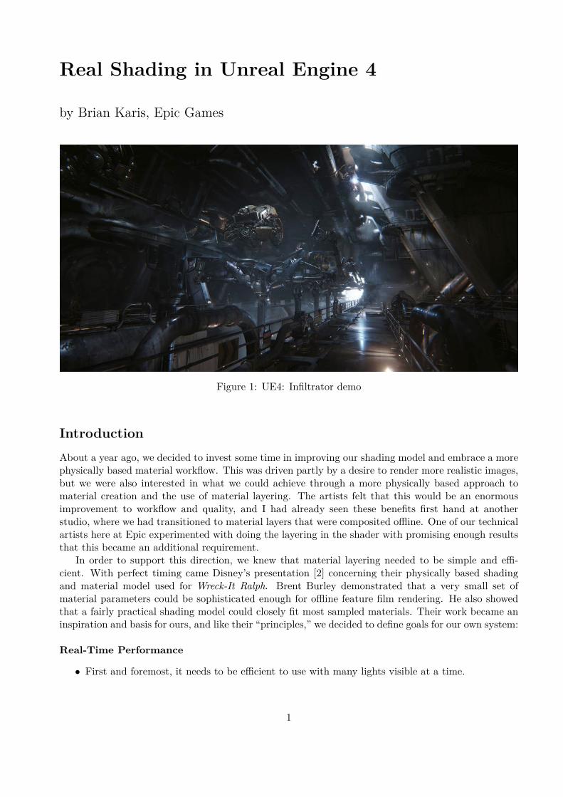
Figure 1: UE4: Infiltrator demo
IntroductionAbout a year ago, we decided to invest some time in improving our shading model and embrace a morephysically based material workflow. This was driven partly by a desire to render more realistic images,but we were also interested in what we could achieve through a more physically based approach tomaterial creation and the use of material layering. The artists felt that this would be an enormousimprovement to workflow and quality, and I had already seen these benefits first hand at anotherstudio, where we had transitioned to material layers that were composited offline. One of our technicalartists here at Epic experimented with doing the layering in the shader with promising enough resultsthat this became an additional requirement.
In order to support this direction, we knew that material layering needed to be simple and effi-cient. With perfect timing came Disney’s presentation [2] concerning their physically based shadingand material model used for Wreck-It Ralph. Brent Burley demonstrated that a very small set ofmaterial parameters could be sophisticated enough for offline feature film rendering. He also showedthat a fairly practical shading model could closely fit most sampled materials. Their work became aninspiration and basis for ours, and like their “principles,” we decided to define goals for our own system:
Real-Time Performance
• First and foremost, it needs to be efficient to use with many lights visible at a time.
1
Reduced Complexity
• There should be as few parameters as possible. A large array of parameters either results indecision paralysis, trial and error, or interconnected properties that require many values to bechanged for a single intended effect.
• We need to be able to use image-based lighting and analytic light sources interchangeably, soparameters must behave consistently across all light types.
Intuitive Interface
• We prefer simple-to-understand values, as opposed to physical ones such as index of refraction.
Perceptually Linear
• We wish to support layering through masks, but we can only afford to shade once per pixel. Thismeans that parameter-blended shading must match blending of the shaded results as closely aspossible.
Easy to Master
• We would like to avoid the need for technical understanding of dielectrics and conductors, as wellas minimize the effort required to create basic physically plausible materials.
Robust
• It should be difficult to mistakenly create physically implausible materials.
• All combinations of parameters should be as robust and plausible as possible.
Expressive
• Deferred shading limits the number of shading models we can have, so our base shading modelneeds to be descriptive enough to cover 99% of the materials that occur in the real world.
• All layerable materials need to share the same set of parameters in order to blend between them.
Flexible
• Other projects and licensees may not share the same goal of photorealism, so it needs to beflexible enough to enable non-photorealistic rendering.
Shading ModelDiffuse BRDFWe evaluated Burley’s diffuse model but saw only minor differences compared to Lambertian diffuse(Equation 1), so we couldn’t justify the extra cost. In addition, any more sophisticated diffuse modelwould be difficult to use efficiently with image-based or spherical harmonic lighting. As a result, wedidn’t invest much effort in evaluating other choices.
f(l,v) = cdiffπ
(1)
Where cdiff is the diffuse albedo of the material.
2
Microfacet Specular BRDFThe general Cook-Torrance [5, 6] microfacet specular shading model is:
f(l,v) = D(h)F (v,h)G(l,v,h)4 (n · l) (n · v) (2)
See [9] in this course for extensive details.We started with Disney’s model and evaluated the importance of each term compared with more
efficient alternatives. This was more difficult than it sounds; published formulas for each term don’tnecessarily use the same input parameters which is vital for correct comparison.
Specular DFor the normal distribution function (NDF), we found Disney’s choice of GGX/Trowbridge-Reitz tobe well worth the cost. The additional expense over using Blinn-Phong is fairly small, and the distinct,natural appearance produced by the longer “tail” appealed to our artists. We also adopted Disney’sreparameterization of α = Roughness2.
D(h) = α2
π ((n · h)2 (α2 − 1) + 1)2(3)
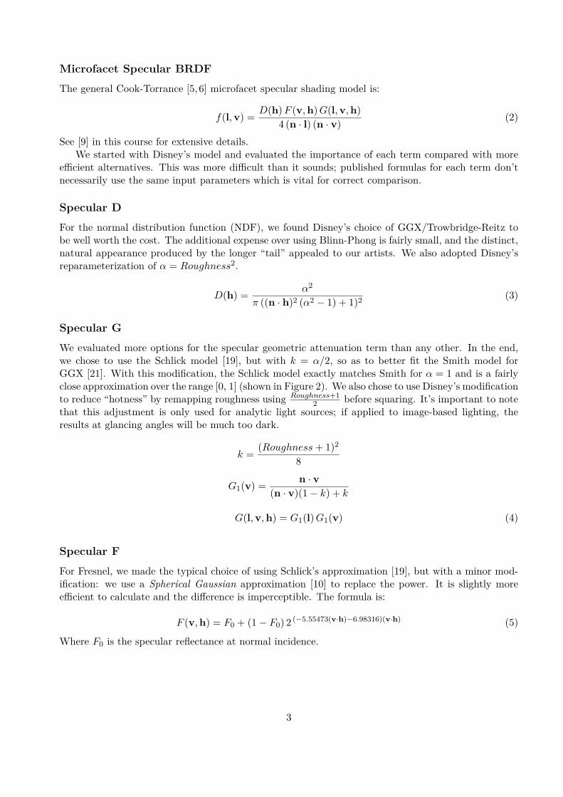
Specular GWe evaluated more options for the specular geometric attenuation term than any other. In the end,we chose to use the Schlick model [19], but with k = α/2, so as to better fit the Smith model forGGX [21]. With this modification, the Schlick model exactly matches Smith for α = 1 and is a fairlyclose approximation over the range [0, 1] (shown in Figure 2). We also chose to use Disney’s modificationto reduce “hotness” by remapping roughness using Roughness+1
2 before squaring. It’s important to notethat this adjustment is only used for analytic light sources; if applied to image-based lighting, theresults at glancing angles will be much too dark.
k =(Roughness+ 1)2
8
G1(v) =n · v
(n · v)(1− k) + k
G(l,v,h) = G1(l)G1(v) (4)
Specular FFor Fresnel, we made the typical choice of using Schlick’s approximation [19], but with a minor mod-ification: we use a Spherical Gaussian approximation [10] to replace the power. It is slightly moreefficient to calculate and the difference is imperceptible. The formula is:
F (v,h) = F0 + (1− F0) 2(−5.55473(v·h)−6.98316)(v·h) (5)
Where F0 is the specular reflectance at normal incidence.
3
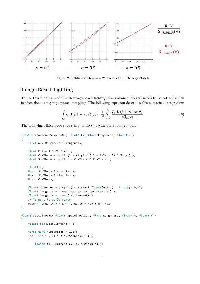
Figure 2: Schlick with k = α/2 matches Smith very closely
Image-Based LightingTo use this shading model with image-based lighting, the radiance integral needs to be solved, whichis often done using importance sampling. The following equation describes this numerical integration:∫
H
Li(l)f(l,v) cos θldl ≈ 1
N
N∑k=1
Li(lk)f(lk,v) cos θlkp(lk,v)
(6)
The following HLSL code shows how to do this with our shading model:
float3 ImportanceSampleGGX( float2 Xi, float Roughness, float3 N ){
float a = Roughness * Roughness;
float Phi = 2 * PI * Xi.x;float CosTheta = sqrt( (1 - Xi.y) / ( 1 + (a*a - 1) * Xi.y ) );float SinTheta = sqrt( 1 - CosTheta * CosTheta );
float3 H;H.x = SinTheta * cos( Phi );H.y = SinTheta * sin( Phi );H.z = CosTheta;
float3 UpVector = abs(N.z) < 0.999 ? float3(0,0,1) : float3(1,0,0);float3 TangentX = normalize( cross( UpVector, N ) );float3 TangentY = cross( N, TangentX );// Tangent to world spacereturn TangentX * H.x + TangentY * H.y + N * H.z;
}
float3 SpecularIBL( float3 SpecularColor, float Roughness, float3 N, float3 V ){
float3 SpecularLighting = 0;
const uint NumSamples = 1024;for( uint i = 0; i < NumSamples; i++ ){
float2 Xi = Hammersley( i, NumSamples );
4

float3 H = ImportanceSampleGGX( Xi, Roughness, N );float3 L = 2 * dot( V, H ) * H - V;
float NoV = saturate( dot( N, V ) );float NoL = saturate( dot( N, L ) );float NoH = saturate( dot( N, H ) );float VoH = saturate( dot( V, H ) );
if( NoL > 0 ){
float3 SampleColor = EnvMap.SampleLevel( EnvMapSampler, L, 0 ).rgb;
float G = G_Smith( Roughness, NoV, NoL );float Fc = pow( 1 - VoH, 5 );float3 F = (1 - Fc) * SpecularColor + Fc;
// Incident light = SampleColor * NoL// Microfacet specular = D*G*F / (4*NoL*NoV)// pdf = D * NoH / (4 * VoH)SpecularLighting += SampleColor * F * G * VoH / (NoH * NoV);
}}
return SpecularLighting / NumSamples;}
Even with importance sampling, many samples still need to be taken. The sample count can bereduced significantly by using mip maps [3], but counts still need to be greater than 16 for sufficientquality. Because we blend between many environment maps per pixel for local reflections, we can onlypractically afford a single sample for each.
Split Sum ApproximationTo achieve this, we approximate the above sum by splitting it into two sums. Each separate sum canthen be precalculated. This approximation is exact for a constant Li(l) and fairly accurate for commonenvironments.
1
N
N∑k=1
Li(lk)f(lk,v) cos θlkp(lk,v)
≈
(1
N
N∑k=1
Li(lk))(
1
N
N∑k=1
f(lk,v) cos θlkp(lk,v)
)(7)
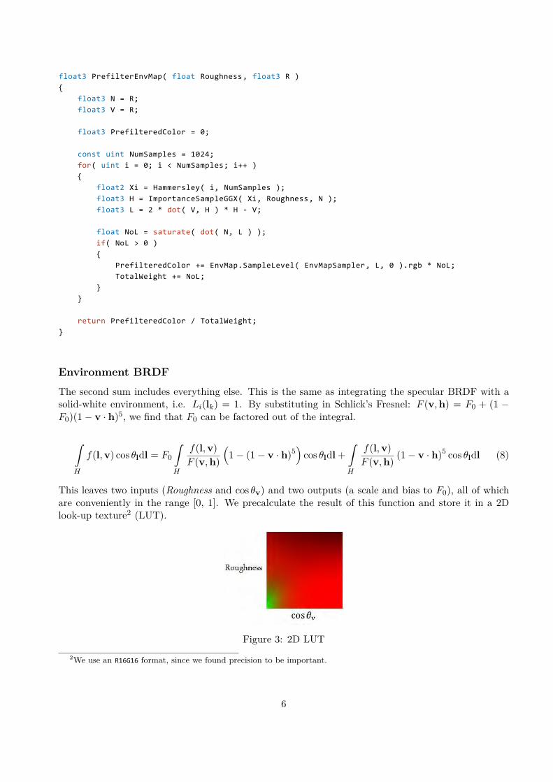
Pre-Filtered Environment MapWe pre-calculate the first sum for different roughness values and store the results in the mip-maplevels of a cubemap. This is the typical approach used by much of the game industry [1, 9]. Oneminor difference is that we convolve the environment map with the GGX distribution of our shadingmodel using importance sampling. Since it’s a microfacet model, the shape of the distribution changesbased on viewing angle to the surface, so we assume that this angle is zero, i.e. n = v = r. Thisisotropic assumption is a second source of approximation and it unfortunately means we don’t getlengthy reflections at grazing angles. Compared with the split sum approximation, this is actually thelarger source of error for our IBL solution. As shown in the code below, we have found weighting bycos θlk achieves better results1.
1This weighting is not present in Equation 7, which is left in a simpler form
5
float3 PrefilterEnvMap( float Roughness, float3 R ){
float3 N = R;float3 V = R;
float3 PrefilteredColor = 0;
const uint NumSamples = 1024;for( uint i = 0; i < NumSamples; i++ ){
float2 Xi = Hammersley( i, NumSamples );float3 H = ImportanceSampleGGX( Xi, Roughness, N );float3 L = 2 * dot( V, H ) * H - V;
float NoL = saturate( dot( N, L ) );if( NoL > 0 ){
PrefilteredColor += EnvMap.SampleLevel( EnvMapSampler, L, 0 ).rgb * NoL;TotalWeight += NoL;
}}
return PrefilteredColor / TotalWeight;}
Environment BRDFThe second sum includes everything else. This is the same as integrating the specular BRDF with asolid-white environment, i.e. Li(lk) = 1. By substituting in Schlick’s Fresnel: F (v,h) = F0 + (1 −F0)(1− v · h)5, we find that F0 can be factored out of the integral.
∫H
f(l,v) cos θldl = F0
∫H
f(l,v)F (v,h)
(1− (1− v · h)5
)cos θldl +
∫H
f(l,v)F (v,h) (1− v · h)5 cos θldl (8)
This leaves two inputs (Roughness and cos θv) and two outputs (a scale and bias to F0), all of whichare conveniently in the range [0, 1]. We precalculate the result of this function and store it in a 2Dlook-up texture2 (LUT).
Figure 3: 2D LUT2We use an R16G16 format, since we found precision to be important.
6

After completing this work, we discovered both existing and concurrent research that lead toalmost identical solutions to ours. Whilst Gotanda used a 3D LUT [8], Drobot optimized this to a 2DLUT [7], in much the same way that we did. Additionally—as part of this course—Lazarov goes onestep further [11], by presenting a couple of analytical approximations to a similar integral3.
float2 IntegrateBRDF( float Roughness, float NoV ){
float3 V;V.x = sqrt( 1.0f - NoV * NoV ); // sinV.y = 0;V.z = NoV; // cos
float A = 0;float B = 0;
const uint NumSamples = 1024;for( uint i = 0; i < NumSamples; i++ ){
float2 Xi = Hammersley( i, NumSamples );float3 H = ImportanceSampleGGX( Xi, Roughness, N );float3 L = 2 * dot( V, H ) * H - V;
float NoL = saturate( L.z );float NoH = saturate( H.z );float VoH = saturate( dot( V, H ) );
if( NoL > 0 ){
float G = G_Smith( Roughness, NoV, NoL );
float G_Vis = G * VoH / (NoH * NoV);float Fc = pow( 1 - VoH, 5 );A += (1 - Fc) * G_Vis;B += Fc * G_Vis;
}}
return float2( A, B ) / NumSamples;}
Finally, to approximate the importance sampled reference, we multiply the two pre-calculated sums:
float3 ApproximateSpecularIBL( float3 SpecularColor, float Roughness, float3 N, float3 V ){
float NoV = saturate( dot( N, V ) );float3 R = 2 * dot( V, N ) * N - V;
float3 PrefilteredColor = PrefilterEnvMap( Roughness, R );float2 EnvBRDF = IntegrateBRDF( Roughness, NoV );
return PrefilteredColor * ( SpecularColor * EnvBRDF.x + EnvBRDF.y );}
3Their shading model uses different D and G functions.
7

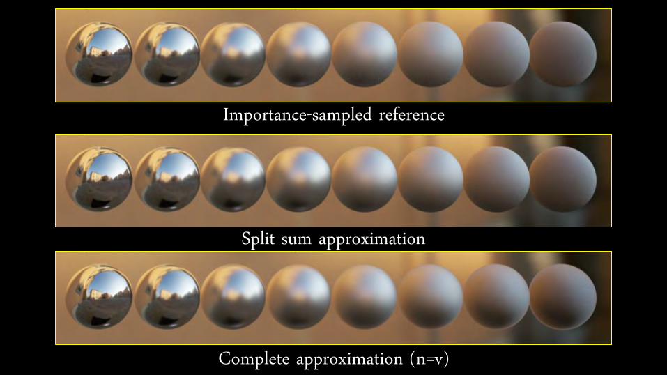
Figure 4: Reference at top, split sum approximation in the middle, full approximation including n = vassumption at the bottom. The radially symmetric assumption introduces the most error but thecombined approximation is still very similar to the reference.
Figure 5: Same comparison as Figure 4 but with a dielectric.
8
Material ModelOur material model is a simplification of Disney’s, with an eye towards efficiency for real-time ren-dering. Limiting the number of parameters is extremely important for optimizing G-Buffer space,reducing texture storage and access, and minimizing the cost of blending material layers in the pixelshader.
The following is our base material model:
BaseColor Single color. Easier concept to understand.Metallic No need to understand dielectric and conductor reflectance, so less room for error.Roughness Very clear in its meaning, whereas gloss always needs explaining.Cavity Used for small-scale shadowing.
BaseColor, Metallic, and Roughness are all the same as Disney’s model, but Cavity parameter wasn’tpresent, so it deserves explanation. Cavity is used to specify shadowing from geometry smaller thanour run-time shadowing system can handle, often due to the geometry only being present in the normalmap. Examples are the cracks between floor boards or the seams in clothing.
The most notable omission is the Specular parameter. We actually continued to use this up untilthe completion of our Infiltrator demo, but ultimately we didn’t like it. First off, we feel “specular” isa terrible parameter name which caused much confusion and was somewhat harmful to the transitionfrom artists controlling specular intensity to controlling roughness. Artists and graphics programmersalike commonly forgot its range and assumed that the default was 1, when its actual default was Bur-ley’s 0.5 (corresponding to 4% reflectance). The cases where Specular was used effectively were almostexclusively for the purpose of small scale shadowing. We found variable index of refraction (IOR) to befairly unimportant for nonmetals, so we have recently replaced Specular with the easier to understandCavity parameter. F0 of nonmetals is now a constant 0.04.
The following are parameters from Disney’s model that we chose not to adopt for our base materialmodel and instead treat as special cases:
Subsurface Samples shadow maps differentlyAnisotropy Requires many IBL samplesClearcoat Requires double IBL samplesSheen Not well defined in Burley’s notes
We have not used these special case models in production with the exception of Subsurface which wasused for the ice in our Elemental demo. Additionally we have a shading model specifically for skin. Forthe future we are considering adopting a hybrid deferred/forward shading approach to better supportmore specialized shading models. Currently with our purely deferred shading approach, differentshading models are handled with a dynamic branch from a shading model id stored in the G-Buffer.
Experiences
There is one situation I have seen a number of times now. I will tell artists beginning the transitionto using varying roughness, “Use Roughness like you used to use SpecularColor” and soon after I hearwith excited surprise: “It works!” But an interesting comment that has followed is: “Roughness feelsinverted.” It turns out that artists want to see the texture they author as brighter texels equals brighterspecular highlights. If the image stores roughness, then bright equates to rougher, which will lead toless intense highlights.
9

A question I have received countless times is: “Is Metallic binary?,” to which I’d originally explainthe subtleties of mixed or layered materials. I have since learned that it’s best to just say “Yes!” Thereason is that artists at the beginning were reluctant to set parameters to absolutes; very commonly Iwould find metals with Metallic values of 0.8. Material layers—discussed next—should be the way todescribe 99% of cases where Metallic would not be either 0 or 1.
We had some issues during the transition, in the form of materials that could no longer be repli-cated. The most important set of these came from Fortnite, a game currently in production at Epic.Fortnite has a non-photorealistic art direction and purposefully uses complementary colors for diffuseand specular reflectance, something that is not physically plausible and intentionally cannot be rep-resented in our new material model. After long discussions, we decided to continue to support theold DiffuseColor/SpecularColor as an engine switch in order to maintain quality in Fortnite, since itwas far into development. However, we don’t feel that the new model precludes non-photorealisticrendering as demonstrated by Disney’s use in Wreck-It Ralph, so we intend to use it for all futureprojects.
Material LayeringBlending material layers which are sourced from a shared library provides a number of benefits overour previous approach, which was to specify material parameters individually with the values comingfrom textures authored for each specific model:
• Reuses work across a number of assets.
• Reduces complexity for a single asset.
• Unifies and centralizes the materials defining the look of the game, allowing easier art and techdirection.
To fully embrace this new workflow, we needed to rethink our tools. Unreal Engine has featureda node graph based material editor since early in UE3’s lifetime. This node graph specifies inputs(textures, constants), operations, and outputs, which are compiled into shader code.
Although material layering was a primary goal of much of this work, surprisingly very little neededto be added tool-side to support the authoring and blending of material layers. Sections of node graphsin UE4’s material editor could already be grouped into functions and used from multiple materials.This functionality is a natural fit for implementing a material layer. Keeping material layers insideour node-based editor, instead of as a fixed function system on top, allowed layers to be mapped andcombined in a programmable way.
To streamline the workflow, we added a new data type, material attributes, that holds all of thematerials output data. This new type, like our other types, can be passed in and out of materialfunctions as single pins, passed along wires, and outputted directly. With these changes, materiallayers can be dragged in as inputs, combined, manipulated and output in the same way that textureswere previously. In fact, most material graphs tend to be simpler since the adoption of layers as theprimary things custom to a particular material are how layers are mapped and blended. This is farsimpler than the parameter specific manipulation that used to exist.
Due to having a small set of perceptually linear material parameters, it is actually practical toblend layers entirely within the shader. We feel this offers a substantial increase in quality over apurely offline composited system. The apparent resolution of texture data can be extremely high dueto being able to map data at different frequencies: per vertex or low frequency texture data can beunique, layer blend masks, normal maps and cavity maps are specified per mesh, and material layersare tiled across the surface of the mesh. More advanced cases may use even more frequencies. Although
10

Figure 6: Simple material layering in the UE4 material editor
we are practically limited in the number of layers we can use due to shader cost, our artists have notyet found the limitation problematic.
An area that is cause for concern is that the artists in cases have worked around the in-shaderlayering limitations by splitting a mesh into multiple sections, resulting in more draw calls. Althoughwe expect better draw call counts in UE4 due to CPU side code optimizations, this seems like it maybe a source of problems in the future. An area we haven’t investigated yet is the use of dynamicbranching to reduce the shader cost in areas where a layer has 100% coverage.
So far, our experience with material layers has been extremely positive. We have seen both pro-ductivity gains and large improvements in quality. We wish to improve the artist interface to thelibrary of material layers by making it easier to find and preview layers. We also intend to investigatean offline compositing/baking system in addition to our current run-time system, to support a largernumber of layers and offer better scalability.
Figure 7: Many material layers swapped and blended with rust.
11
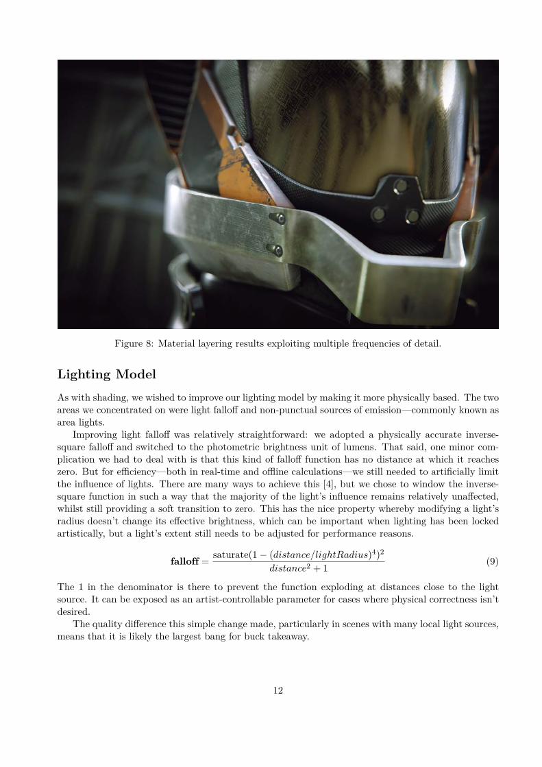
Figure 8: Material layering results exploiting multiple frequencies of detail.
Lighting ModelAs with shading, we wished to improve our lighting model by making it more physically based. The twoareas we concentrated on were light falloff and non-punctual sources of emission—commonly known asarea lights.
Improving light falloff was relatively straightforward: we adopted a physically accurate inverse-square falloff and switched to the photometric brightness unit of lumens. That said, one minor com-plication we had to deal with is that this kind of falloff function has no distance at which it reacheszero. But for efficiency—both in real-time and offline calculations—we still needed to artificially limitthe influence of lights. There are many ways to achieve this [4], but we chose to window the inverse-square function in such a way that the majority of the light’s influence remains relatively unaffected,whilst still providing a soft transition to zero. This has the nice property whereby modifying a light’sradius doesn’t change its effective brightness, which can be important when lighting has been lockedartistically, but a light’s extent still needs to be adjusted for performance reasons.
falloff = saturate(1− (distance/lightRadius)4)2
distance2 + 1(9)
The 1 in the denominator is there to prevent the function exploding at distances close to the lightsource. It can be exposed as an artist-controllable parameter for cases where physical correctness isn’tdesired.
The quality difference this simple change made, particularly in scenes with many local light sources,means that it is likely the largest bang for buck takeaway.
12

Figure 9: Inverse square falloff achieves more natural results
Area LightsArea light sources don’t just generate more realistic images. They are also fairly important whenusing physically based materials. We found that without them, artists tended to intuitively avoidpainting very low roughness values, since this resulted in infinitesimal specular highlights, which lookedunnatural. Essentially, they were trying to reproduce the effect of area lighting from punctual sources 4.
Unfortunately, this reaction leads to a coupling between shading and lighting, breaking one of thecore principles of physically based rendering: that materials shouldn’t need to be modified when usedin a different lighting environment from where they were created.
Area lights are an active area of research. In offline rendering, the common solution is to lightfrom many points on the surface of the light source—either using uniform sampling or importancesampling [12] [20]. This is completely impractical for real-time rendering. Before discussing possiblesolutions, here were our requirements:
• Consistent material appearance
– The amount of energy evaluated with the Diffuse BRDF and the Specular BRDF cannot besignificantly different.
• Approaches point light model as the solid angle approaches zero
– We don’t want to lose any aspect of our shading model to achieve this.
• Fast enough to use everywhere
– Otherwise, we cannot solve the aforementioned “biased roughness” issue.
4This tallies with observations from other developers [7,8].
13
Billboard ReflectionsBillboard reflections [13] are a form of IBL that can be used for discrete light sources. A 2D image,which stores emitted light, is mapped to a rectangle in 3d space. Similar to environment map pre-filtering, the image is pre-filtered for different-sized specular distribution cones. Calculating specularshading from this image can be thought of as a form of cone tracing, where a cone approximates thespecular NDF. The ray at the center of the cone is intersected with the plane of the billboard. Thepoint of intersection in image space is then used as the texture coordinates, and the radius of the coneat the intersection is used to derive an appropriate pre-filtered mip level. Sadly, while images canexpress very complex area light sources in a straightforward manner, billboard reflections fail to fulfillour second requirement for multiple reasons:
• The image is pre-filtered on a plane, so there is a limited solid angle that can be represented inimage space.
• There is no data when the ray doesn’t intersect the plane.
• The light vector, l, is unknown or assumed to be the reflection vector.
Cone IntersectionCone tracing does not require pre-filtering; it can be done analytically. A version we experimentedwith traced a cone against a sphere using Oat’s cone-cone intersection equation [15], but it was fartoo expensive to be practical. An alternative method presented recently by Drobot [7] intersected thecone with a disk facing the shading point. A polynomial approximating the NDF is then piece-wiseintegrated over the intersecting area.
With Drobot’s recent advancements, this seems to be an interesting area for research, but in itscurrent form, it doesn’t fulfill our requirements. Due to using a cone, the specular distribution mustbe radially symmetric. This rules out stretched highlights, a very important feature of the microfacetspecular model. Additionally, like billboard reflections, there isn’t a defined light vector required bythe shading model.
Specular D ModificationAn approach we presented last year [14] is to modify the specular distribution based on the solid angleof the light source. The theory behind this is to consider the light source’s distribution to be the sameas D(h) for a corresponding cone angle. Convolving one distribution by the other can be approximatedby adding the angles of both cones to derive a new cone. To achieve this, convert α from Equation 3into an effective cone angle, add the angle of the light source, and convert back. This α′ is now usedin place of α. We use the following approximation to do this:
α′ = saturate(α+
sourceRadius
3 ∗ distance
)(10)
Although efficient, this technique unfortunately doesn’t fulfill our first requirement, as very glossymaterials appear rough when lit with large area lights. This may sound obvious, but the techniqueworks a great deal better when the specular NDF is compact—Blinn-Phong, for instance—therebybetter matching the light source’s distribution. For our chosen shading model (based on GGX), it isn’tviable.
14
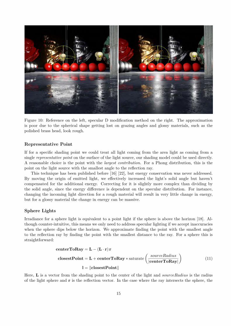
Figure 10: Reference on the left, specular D modification method on the right. The approximationis poor due to the spherical shape getting lost on grazing angles and glossy materials, such as thepolished brass head, look rough.
Representative PointIf for a specific shading point we could treat all light coming from the area light as coming from asingle representative point on the surface of the light source, our shading model could be used directly.A reasonable choice is the point with the largest contribution. For a Phong distribution, this is thepoint on the light source with the smallest angle to the reflection ray.
This technique has been published before [16] [22], but energy conservation was never addressed.By moving the origin of emitted light, we effectively increased the light’s solid angle but haven’tcompensated for the additional energy. Correcting for it is slightly more complex than dividing bythe solid angle, since the energy difference is dependent on the specular distribution. For instance,changing the incoming light direction for a rough material will result in very little change in energy,but for a glossy material the change in energy can be massive.
Sphere LightsIrradiance for a sphere light is equivalent to a point light if the sphere is above the horizon [18]. Al-though counter-intuitive, this means we only need to address specular lighting if we accept inaccuracieswhen the sphere dips below the horizon. We approximate finding the point with the smallest angleto the reflection ray by finding the point with the smallest distance to the ray. For a sphere this isstraightforward:
centerToRay = L − (L · r) r
closestPoint = L + centerToRay ∗ saturate(
sourceRadius
|centerToRay|
)l = ∥closestPoint∥
(11)
Here, L is a vector from the shading point to the center of the light and sourceRadius is the radiusof the light sphere and r is the reflection vector. In the case where the ray intersects the sphere, the
15

point calculated will be the closest point on the ray to the center of the sphere. Once normalized, it isidentical.
By moving the origin of emitted light to the sphere’s surface, we have effectively widened thespecular distribution by the sphere’s subtended angle. Although it isn’t a microfacet distribution, thiscan be explained best using a normalized Phong distribution:
Ipoint =p+ 2
2πcosp ϕr (12)
Isphere =
{ p+22π if ϕr < ϕsp+22π cosp (ϕr − ϕs) if ϕr ≥ ϕs
(13)
Here ϕr is the angle between r and L and ϕs is half the sphere’s subtended angle. Ipoint is normalized,meaning the result of integrating it over the hemisphere is 1. Isphere is clearly no longer normalizedand depending on the power p, the integral can be far larger.
Figure 11: Visualization of the widening effect explained with Equation 13
To approximate this increase in energy, we apply the same reasoning used by the specular Dmodification described earlier, where we widened the distribution based on the solid angle of the light.We use the normalization factor for that wider distribution and replace the original normalizationfactor. For GGX the normalization factor is 1
πα2 . To derive an approximate normalization for therepresentative point operation we divide the new widened normalization factor by the original:
SphereNormalization =( α
α′
)2(14)
The results of the representative point method meet all of our requirements. By correctly addressingenergy conservation, materials behave the same regardless of light source size. Glossy materials stillproduce sharp-edged specular highlights, and since it only modifies the inputs to the BRDF, ourshading model is unaffected. Lastly, it is efficient enough to use wherever our artists like.
Tube LightsWhere sphere lights are useful to represent light bulbs, tube lights (capsules) can be useful to representflorescent lights which are quite common in the real world. To start, we solve for tube lights with alength but zero radius, also known as linear lights. Irradiance for a line segment can be integratedanalytically so long as the segment is above the horizon [16,17]:∫ L1
L0
n · L|L|3 dL =
n·L0|L0| +
n·L1|L1|
|L0||L1|+ (L0 · L1)(15)
Where L0 and L1 are vectors from the shading point to the end points of the segment.
16
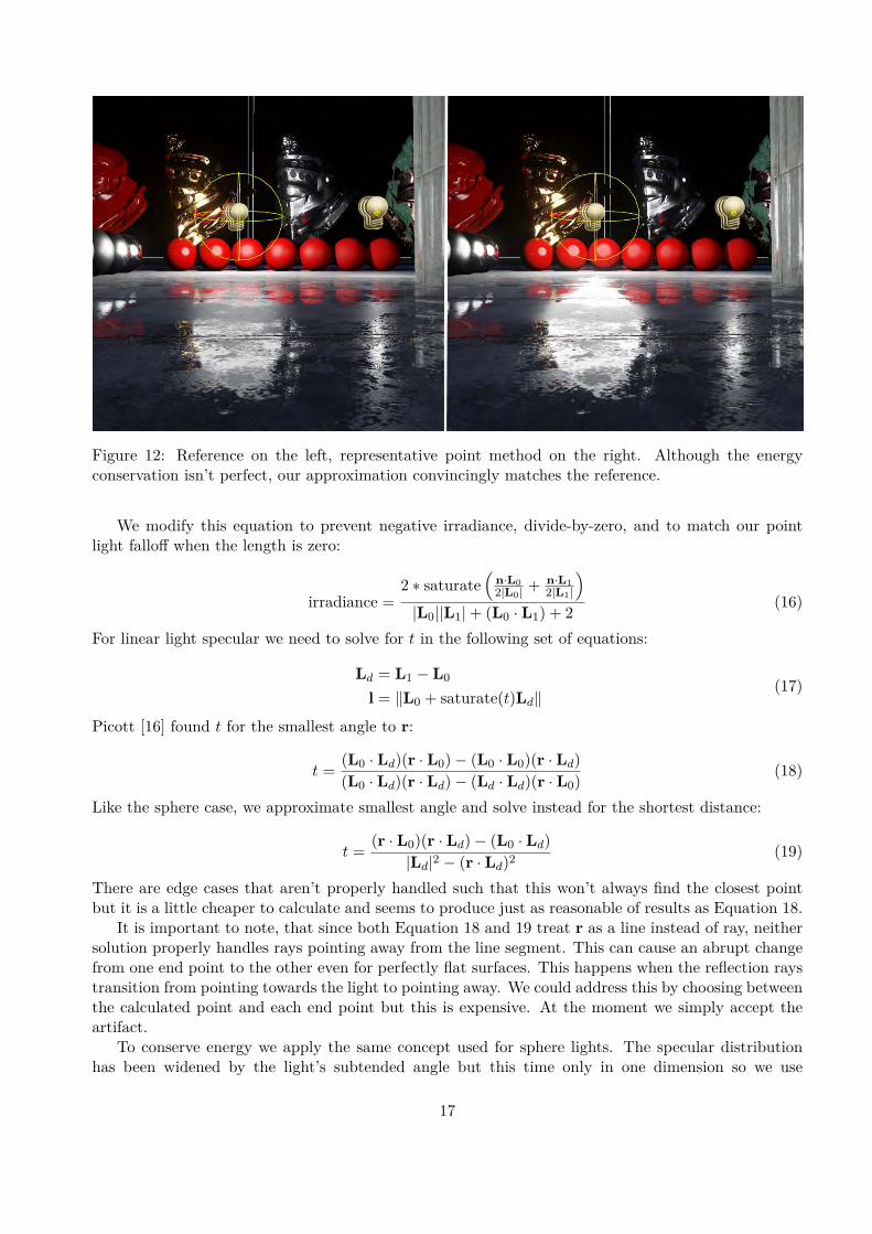
Figure 12: Reference on the left, representative point method on the right. Although the energyconservation isn’t perfect, our approximation convincingly matches the reference.
We modify this equation to prevent negative irradiance, divide-by-zero, and to match our pointlight falloff when the length is zero:
irradiance =2 ∗ saturate
(n·L02|L0| +
n·L12|L1|
)|L0||L1|+ (L0 · L1) + 2
(16)
For linear light specular we need to solve for t in the following set of equations:
Ld = L1 − L0
l = ∥L0 + saturate(t)Ld∥(17)
Picott [16] found t for the smallest angle to r:
t =(L0 · Ld)(r · L0)− (L0 · L0)(r · Ld)
(L0 · Ld)(r · Ld)− (Ld · Ld)(r · L0)(18)
Like the sphere case, we approximate smallest angle and solve instead for the shortest distance:
t =(r · L0)(r · Ld)− (L0 · Ld)
|Ld|2 − (r · Ld)2(19)
There are edge cases that aren’t properly handled such that this won’t always find the closest pointbut it is a little cheaper to calculate and seems to produce just as reasonable of results as Equation 18.
It is important to note, that since both Equation 18 and 19 treat r as a line instead of ray, neithersolution properly handles rays pointing away from the line segment. This can cause an abrupt changefrom one end point to the other even for perfectly flat surfaces. This happens when the reflection raystransition from pointing towards the light to pointing away. We could address this by choosing betweenthe calculated point and each end point but this is expensive. At the moment we simply accept theartifact.
To conserve energy we apply the same concept used for sphere lights. The specular distributionhas been widened by the light’s subtended angle but this time only in one dimension so we use
17

the anisotropic version of GGX [2]. The normalization factor for anisotropic GGX is 1παxαy
whereαx = αy = α in the isotropic case. This gives us:
LineNormalization =α
α′ (20)
Because we are only changing the light’s origin and applying an energy conservation term theseoperations can be accumulated. Doing so with a line segment and a sphere, approximates a convolutionof the shapes and models fairly well the behavior of a tube light. Tube light results are shown in Figure13
Figure 13: Tube light using the representative point method with energy conservation
We have found the representative point method with energy conservation to be effective for simpleshapes and would like to apply it in the future to other shapes beyond spheres and tubes. In particular,we would like to apply it to textured quads to express more complex and multi-colored light sources.
ConclusionOur move to more physically based implementations, in the areas of shading, materials and lighting,has proved to be very successful. It contributed greatly to the visuals of our latest Infiltrator demo andwe plan to use these improvements for all future projects. In fact, in cases where it is practical thesechanges have been integrated into Fortnite, a project well into development before this work began.We intend to continue to improve in these areas with the goals of greater flexibility and scalability withthe goal that all variety of scenes and all levels of hardware can take advantage of physically basedapproaches.
18

AcknowledgmentsI would like to thank Epic Games, in particular everyone on the rendering team who had a hand in thiswork and the artists that have provided direction, feedback, and in the end made beautiful things withit. I would like to give a special thanks to Sebastien Lagarde who found a mistake in my importancesampling math, which when fixed lead to the development of our environment BRDF solution. Neverunderestimate how valuable it can be to have talented licensees around the world looking over the codeyou write. Lastly, I’d like to thank Stephen Hill and Stephen McAuley for their valuable feedback.
19
Bibliography
[1] AMD, CubeMapGen: Cubemap Filtering and Mipchain Generation Tool. http://developer.amd.com/resources/archive/archived-tools/gpu-tools-archive/cubemapgen/
[2] Burley, Brent, “Physically-Based Shading at Disney”, part of “Practical Physically Based Shadingin Film and Game Production”, SIGGRAPH 2012 Course Notes. http://blog.selfshadow.com/publications/s2012-shading-course/
[3] Colbert, Mark, and Jaroslav Krivanek, “GPU-based Importance Sampling”, in Hubert Nguyen,ed., GPU Gems 3, Addison-Wesley, pp. 459–479, 2007. http://http.developer.nvidia.com/GPUGems3/gpugems3_ch20.html
[4] Coffin, Christina, “SPU Based Deferred Shading in Battlefield 3 for Playstation 3”, GameDevelopers Conference, March 2011. http://www.slideshare.net/DICEStudio/spubased-deferred-shading-in-battlefield-3-for-playstation-3
[5] Cook, Robert L., and Kenneth E. Torrance, “A Reflectance Model for Computer Graphics”,Computer Graphics (SIGGRAPH ’81 Proceedings), pp. 307–316, July 1981.
[6] Cook, Robert L., and Kenneth E. Torrance, “A Reflectance Model for Computer Graphics”,ACM Transactions on Graphics, vol. 1, no. 1, pp. 7–24, January 1982. http://graphics.pixar.com/library/ReflectanceModel/
[7] Drobot, Micha l, “Lighting Killzone: Shadow Fall”, Digital Dragons, April 2013. http://www.guerrilla-games.com/publications/
[8] Gotanda, Yoshiharu, “Practical Implementation of Physically-Based Shading Models at tri-Ace”,part of “Physically-Based Shading Models in Film and Game Production”, SIGGRAPH 2010Course Notes. http://renderwonk.com/publications/s2010-shading-course/
[9] Hoffman, Naty, “Background: Physics and Math of Shading”, part of “Physically Based Shad-ing in Theory and Practice”, SIGGRAPH 2013 Course Notes. http://blog.selfshadow.com/publications/s2013-shading-course/
[10] Lagarde, Sebastien, “Spherical Gaussian approximation for Blinn-Phong, Phong and Fresnel”,June 2012. http://seblagarde.wordpress.com/2012/06/03/spherical-gaussien-approximation-for-blinn-phong-phong-and-fresnel/
[11] Lazarov, Dimitar, “Getting More Physical in Call of Duty: Black Ops II”, part of “Physi-cally Based Shading in Theory and Practice”, SIGGRAPH 2013 Course Notes. http://blog.selfshadow.com/publications/s2013-shading-course/
20
[12] Martinez, Adam, “Faster Photorealism in Wonderland: Physically-Based Shading and Lightingat Sony Pictures Imageworks”, part of “Physically-Based Shading Models in Film and Game Pro-duction”, SIGGRAPH 2010 Course Notes. http://renderwonk.com/publications/s2010-shading-course/
[13] Mittring, Martin, and Bryan Dudash, “The Technology Behind the DirectX 11 Unreal EngineSamaritan Demo”, Game Developer Conference 2011. http://udn.epicgames.com/Three/rsrc/Three/DirectX11Rendering/MartinM_GDC11_DX11_presentation.pdf
[14] Mittring, Martin, “The Technology Behind the Unreal Engine 4 Elemental demo”, part of “Ad-vances in Real-Time Rendering in 3D Graphics and Games Course”, SIGGRAPH 2012. http://www.unrealengine.com/files/misc/The_Technology_Behind_the_Elemental_Demo_16x9_(2).pdf
[15] Oat, Chris, “Ambient Aperture Lighting”, SIGGRAPH 2006. http://developer.amd.com/wordpress/media/2012/10/Oat-AmbientApetureLighting.pdf
[16] Picott, Kevin P., “Extensions of the Linear and Area Lighting Models”, Computers and Graphics,Volume 12 Issue 2, March 1992, pp. 31-38. http://dx.doi.org/10.1109/38.124286
[17] Poulin, Pierre, and John Amanatides, “Shading and Shadowing with Linear Light Sources”,IEEE Computer Graphics and Applications, 1991. http://www.cse.yorku.ca/~amana/research/
[18] Quilez, Inigo, “Spherical ambient occlusion”, 2006. http://www.iquilezles.org/www/articles/sphereao/sphereao.htm
[19] Schlick, Christophe, “An Inexpensive BRDF Model for Physically-based Rendering”, ComputerGraphics Forum, vol. 13, no. 3, Sept. 1994, pp. 149–162. http://dept-info.labri.u-bordeaux.fr/~schlick/DOC/eur2.html
[20] Snow, Ben, “Terminators and Iron Men: Image-based lighting and physical shading at ILM”,part of “Physically-Based Shading Models in Film and Game Production”, SIGGRAPH 2010Course Notes. http://renderwonk.com/publications/s2010-shading-course/
[21] Walter, Bruce, Stephen R. Marschner, Hongsong Li, Kenneth E. Torrance, “Microfacet Modelsfor Refraction through Rough Surfaces”, Eurographics Symposium on Rendering (2007), 195–206,June 2007. http://www.cs.cornell.edu/~srm/publications/EGSR07-btdf.html
[22] Wang, Lifeng, Zhouchen Lin, Wenle Wang, and Kai Fu, “One-Shot Approximate Local Shading”2006.
21
Real Shading in Unreal Engine 4 Brian Karis ([email protected])

Goals • More realistic image • Material layering
– Better workflow – Blended in shader
• Timely inspiration from Disney – Presented in this course last year

Overview • Shading model • Material model • Lighting model

Shading Model
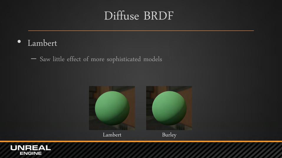
• Lambert – Saw little effect of more sophisticated models
Diffuse BRDF
Lambert Burley
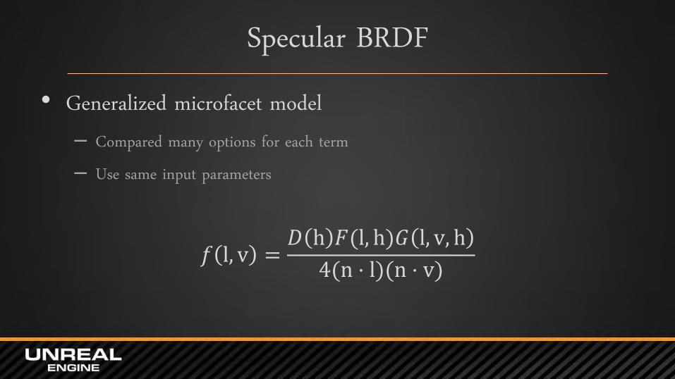
Specular BRDF • Generalized microfacet model
– Compared many options for each term – Use same input parameters
𝑓 l, v =𝐷 h 𝐹(l, h)𝐺 l, v, h
4(n ⋅ l)(n ⋅ v)

Specular distribution • Trowbridge-Reitz (GGX)
– Fairly cheap – Longer tail looks much more natural
GGX Blinn-Phong
𝑓 l, v =𝐷 h 𝐹(l, h)𝐺 l, v, h
4(n ⋅ l)(n ⋅ v)
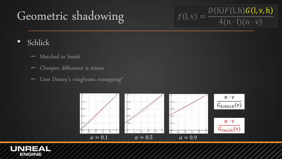
Geometric shadowing • Schlick
– Matched to Smith – Cheaper, difference is minor – Uses Disney’s roughness remapping*
n ⋅ v
𝐺𝑆𝑐ℎ𝑙𝑖𝑐𝑘(v)
𝛼 = 0.1 𝛼 = 0.5 𝛼 = 0.9
𝑓 l, v =𝐷 h 𝐹(l, h)𝐺 l, v, h
4(n ⋅ l)(n ⋅ v)
n ⋅ v
𝐺𝑆𝑚𝑖𝑡ℎ(v)
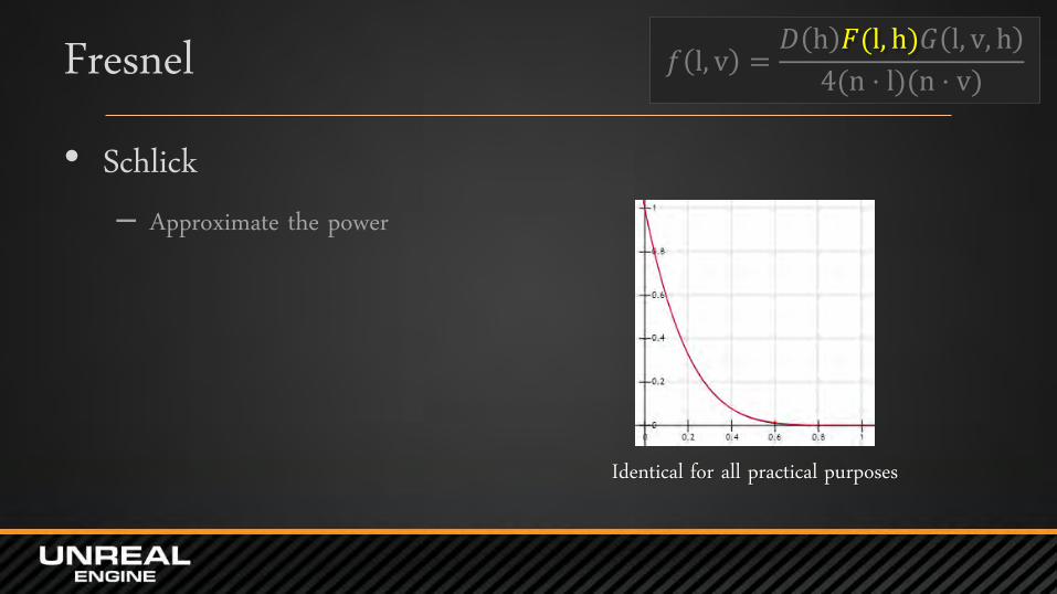
Fresnel • Schlick
– Approximate the power
Identical for all practical purposes
𝑓 l, v =𝐷 h 𝐹(l, h)𝐺 l, v, h
4(n ⋅ l)(n ⋅ v)

Image-based lighting : Problem • Only use single sample per environment map • Match importance-sampled reference
𝐿𝑖 l 𝑓 l, v 𝑐𝑜𝑠 𝜃l 𝑑l
𝐻
≈1
𝑁 𝐿𝑖 l𝑘 𝑓 l𝑘 , v 𝑐𝑜𝑠 𝜃l𝑘
𝑝 l𝑘 , v
𝑁
𝑘=1

Image-based lighting : Solution • Same as Dimitar’s: split the sum • Pre-calculate both parts
1
𝑁 𝐿𝑖 l𝑘 𝑓 l𝑘 , v cos 𝜃l𝑘
𝑝 l𝑘 , 𝑣
𝑁
𝑘=1
≈1
𝑁 𝐿𝑖 l𝑘
𝑁
𝑘=1
1
𝑁 𝑓(l𝑘 , v) cos 𝜃l𝑘𝑝(l𝑘 , v)
𝑁
𝑘=1
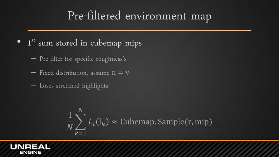
Pre-filtered environment map • 1st sum stored in cubemap mips
– Pre-filter for specific roughness’s – Fixed distribution, assume n = v – Loses stretched highlights
1
𝑁 𝐿𝑖 l𝑘
𝑁
𝑘=1
≈ Cubemap. Sample(r,mip)

Environment BRDF • 2nd sum stored in 2D lookup texture (LUT)
1
𝑁 𝑓(l𝑘 , v) cos 𝜃l𝑘𝑝(l𝑘 , v)
𝑁
𝑘=1
= LUT. r ∗ 𝐹0 + LUT. g
cos 𝜃v
Roughness

Importance-sampled reference

Split sum approximation

Complete approximation (n=v)
Complete approximation (n=v)
Importance-sampled reference
Split sum approximation

Material Model
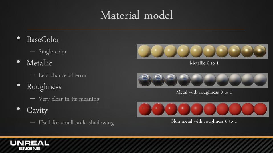
Material model • BaseColor
– Single color • Metallic
– Less chance of error • Roughness
– Very clear in its meaning • Cavity
– Used for small scale shadowing
Metallic 0 to 1
Non-metal with roughness 0 to 1
Metal with roughness 0 to 1

Material model lessons • Specular parameter is confusing
– Not really needed – Replaced with Cavity
DiffuseColor SpecularColor SpecularPower
BaseColor Metallic Specular Roughness
BaseColor Metallic Roughness Cavity
Samaritan Infiltrator Now

Material layering • TODO:anotherimage
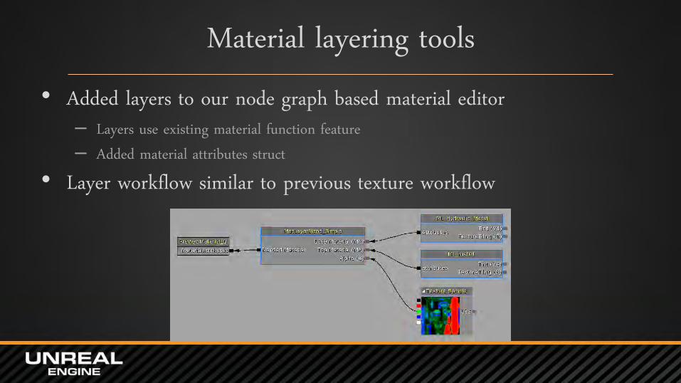
Material layering tools • Added layers to our node graph based material editor
– Layers use existing material function feature – Added material attributes struct
• Layer workflow similar to previous texture workflow

Material layering

Material layering

Lighting Model

Inverse square falloff
Old falloff Inverse square

Area Lights
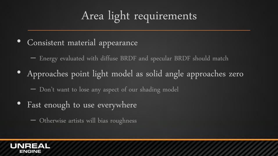
Area light requirements • Consistent material appearance
– Energy evaluated with diffuse BRDF and specular BRDF should match
• Approaches point light model as solid angle approaches zero – Don’t want to lose any aspect of our shading model
• Fast enough to use everywhere – Otherwise artists will bias roughness

Specular D modification • Widen specular distribution by light’s solid angle
– We presented this last year
• Problems – Glossy surfaces don’t look glossy anymore

Reference Specular D modification

Representative point • Pick one representative point on light source shape • Shading model can be used directly • Point with largest contribution is a good choice • Approximate using smallest angle to reflection ray
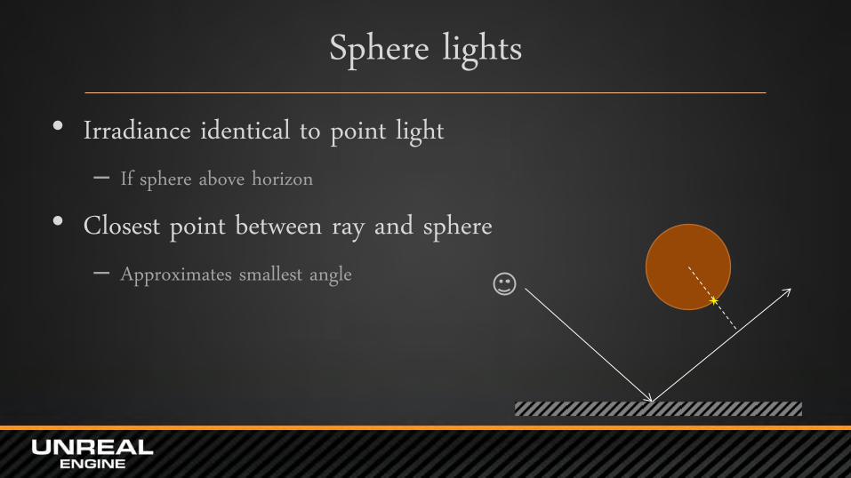
Sphere lights • Irradiance identical to point light
– If sphere above horizon
• Closest point between ray and sphere – Approximates smallest angle
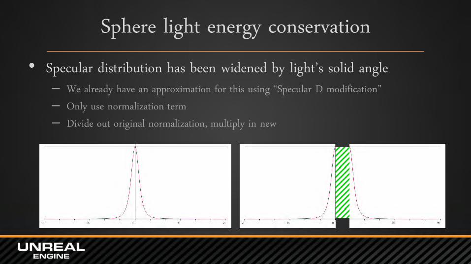
Sphere light energy conservation • Specular distribution has been widened by light’s solid angle
– We already have an approximation for this using “Specular D modification” – Only use normalization term – Divide out original normalization, multiply in new

Reference Representative point

Representative point applied to Tube Lights
In the course notes • Tons of extra stuff
– Importance sampling code – Area light formulas – Lots of math

Thanks • Epic
– Rendering team – All the artists making me look good
• Special thanks to Sébastien Lagarde • Stephen Hill and Stephen McAuley for valuable input
