Real-Time Collision Forecastingfrom Monocular Video

Aashi Manglik

CMU-RI-TR-19-42

July 2, 2019

The Robotics InstituteCarnegie Mellon University

Pittsburgh, Pennsylvania 15213

Thesis Committee:Prof. Kris M. Kitani, Chair, CMU

Prof. Aaron Steinfeld, CMUIshani Chatterjee, CMU

Thesis proposal submitted in partial fulfillment of therequirements for the degree of Master of Science in Robotics

c©Aashi Manglik, 2019

AbstractWe explore the possibility of using a single monocular camera to forecast the time to

collision between a suitcase-shaped robot being pushed by its user and other nearby pedes-trians. We develop a purely image-based deep learning approach that directly estimates thetime to collision without the need of relying on explicit geometric depth estimates or veloc-ity information to predict future collisions. While previous work has focused on detectingimmediate collision in the context of navigating Unmanned Aerial Vehicles, the detectionwas limited to a binary variable (i.e., collision or no collision). We propose a more fine-grained approach to collision forecasting by predicting the exact time to collision in termsof milliseconds, which is more helpful for collision avoidance in the context of dynamicpath planning. To evaluate our method, we have collected a novel large-scale dataset ofover 13,000 indoor video segments each showing a trajectory of at least one person end-ing in a close proximity (a near collision) with the camera mounted on a mobile suitcase-shaped platform. Using this dataset, we do extensive experimentation on different temporalwindows as input using an exhaustive list of state-of-the-art convolutional neural networks(CNNs). Our results show that our proposed multi-stream CNN is the best model for pre-dicting time to near-collision. The average prediction error of our time to near collision is0.75 seconds across the test videos.

I

AcknowledgementI would first like to thank my advisor, Professor Kris Kitani, for giving me the opportu-

nity to work on the CaBot project. Through all the triumphs and failures accompanying thisMaster program, I am glad to have his experience and guidance by my side. I would fur-ther like to thank my thesis committee member, Professor Aaron Steinfeld, for his support,encouragement and valuable feedback along the course of this work and journey ahead.Thanks to Eshed Ohn-Bar for getting me started on this two-year long ride and the insight-ful discussions which helped me overcome any doubts.

I would like to thank Xinshuo Weng for the support during a hard deadline and helpimprove the quality of my work. I would like to thank Ishani Chatterjee whose keen intel-lect has helped me develop deeper understanding of the field. Thanks to all the members ofKLab and Cognitive Assistance Lab for providing a thriving workplace and help me grow.I cannot go without thanking my friends for providing both academic and emotional sup-port in difficult times.

Finally, I would like to express a deep gratitude to my parents and my brother for theirendless support and love.

II

Contents

1 Introduction 1

2 Related Work 32.1 Monocular-Based Collision Avoidance . . . . . . . . . . . . . . . . . . . . . . 32.2 Predicting Time to Collision by Human Trajectory . . . . . . . . . . . . . . . 32.3 Learning Spatio-Temporal Feature Representation . . . . . . . . . . . . . . . 4

3 Dataset 53.1 Hardware Setup . . . . . . . . . . . . . . . . . . . . . . . . . . . . . . . . . . . 53.2 Camera-LIDAR Extrinsic Calibration . . . . . . . . . . . . . . . . . . . . . . . 63.3 Data Collection and Annotation . . . . . . . . . . . . . . . . . . . . . . . . . . 63.4 Comparison with Existing Datasets . . . . . . . . . . . . . . . . . . . . . . . . 7

4 Approach 84.1 Problem Formulation - Classification or Regression? . . . . . . . . . . . . . . 84.2 Network Architecture . . . . . . . . . . . . . . . . . . . . . . . . . . . . . . . . 8

5 Experimental Evaluation 115.1 Initial Experimentation - Classification . . . . . . . . . . . . . . . . . . . . . . 115.2 Regression Experiments - Different temporal windows as input . . . . . . . 145.3 Experimental comparison of architectures . . . . . . . . . . . . . . . . . . . . 145.4 Qualitative Evaluation . . . . . . . . . . . . . . . . . . . . . . . . . . . . . . . 16

6 Conclusion 19

7 Future Work 20

III

Chapter 1

Introduction

Automated collision avoidance technology is an indispensable part of mobile robots. As analternative to traditional approaches using multi-modal sensors, purely image based colli-sion avoidance strategies [9], [17] have recently gained attention in robotics. These image-based approaches use the power of large data to detect immediate collision as a binaryvariable - collision or no collision. In this work, we propose a more fine-grained approachto predict the exact time to collision from images, with a much longer prediction horizon.

A method frequently used for forecasting time to collision is to track the 3D locationof the surrounding pedestrians and extrapolate their trajectories using a constant velocitymodel [21], [14]. When it is possible to use high quality depth imaging devices, this type ofphysics-based modeling can be very accurate. However, physics-based approach can also beprone to failure in the presence of sensor noise and uncertainty in detection of nearby pedes-trians. Small mistakes in the estimation of depth (common to low-cost depth sensors) ornoise in 2D bounding box detection (common to image-based object detection algorithms)can be misinterpreted to be very large changes of velocity. Many physics-based approachescan be brittle in the presence of such noise. Accordingly, errors in either pedestrian detec-tion, tracking or data association can result in very bad future trajectory estimates. Othermore advanced physics-based models and decision-theoretic models also depend heavilyon accurate state estimates of nearby people and can be significantly influenced by sensorand perception algorithm noise. We propose to address the issue of sensor noise and per-ception algorithm noise by directly estimating the time to near-collision from a sequence ofimages.

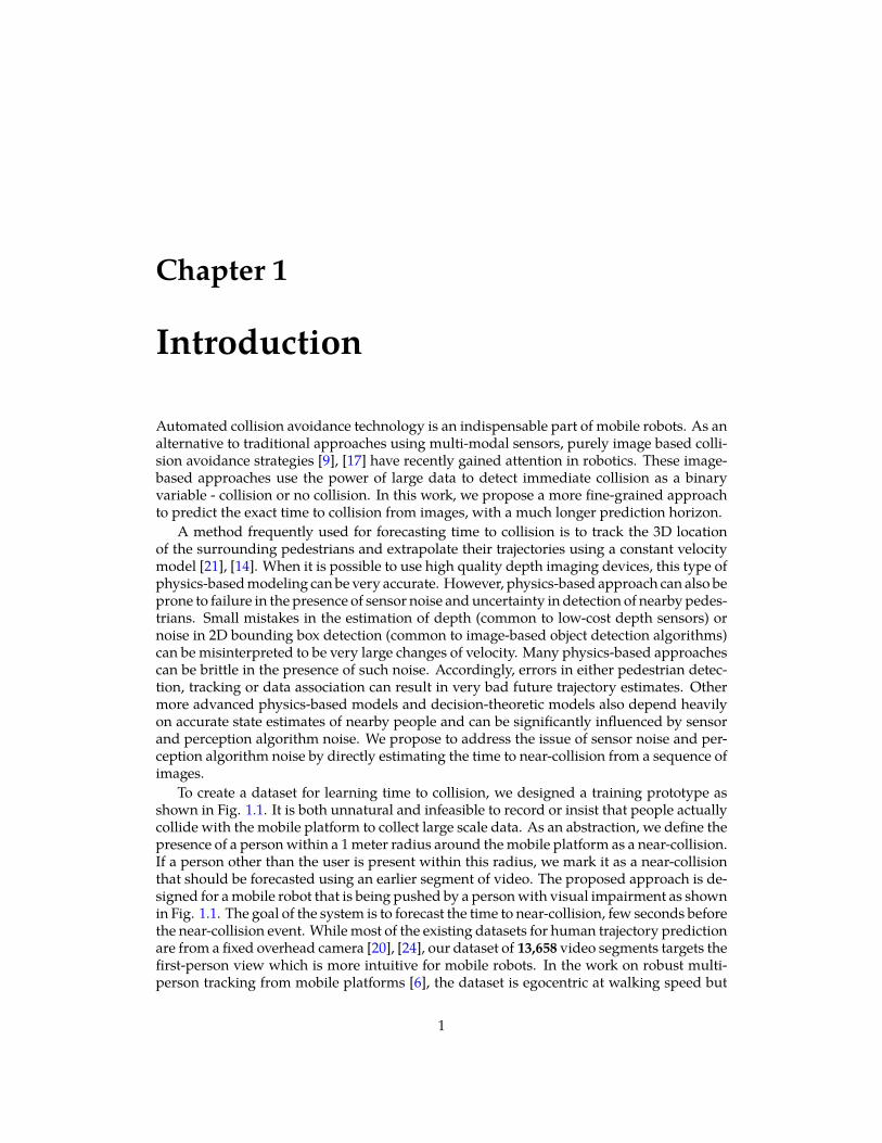
To create a dataset for learning time to collision, we designed a training prototype asshown in Fig. 1.1. It is both unnatural and infeasible to record or insist that people actuallycollide with the mobile platform to collect large scale data. As an abstraction, we define thepresence of a person within a 1 meter radius around the mobile platform as a near-collision.If a person other than the user is present within this radius, we mark it as a near-collisionthat should be forecasted using an earlier segment of video. The proposed approach is de-signed for a mobile robot that is being pushed by a person with visual impairment as shownin Fig. 1.1. The goal of the system is to forecast the time to near-collision, few seconds beforethe near-collision event. While most of the existing datasets for human trajectory predictionare from a fixed overhead camera [20], [24], our dataset of 13,658 video segments targets thefirst-person view which is more intuitive for mobile robots. In the work on robust multi-person tracking from mobile platforms [6], the dataset is egocentric at walking speed but

1

LIDAR

STEREO CAMERA

USER HANDLE

Figure 1.1: The left image shows an assistive suitcase with a camera sensor and speaker toguide people. The right image shows the corresponding suitcase-shaped training prototypemounted with stereo camera and LIDAR for data collection.

with 4788 images it is insufficient to deploy the success of convolutional neural networks.We formulate the forecasting of time to near-collision as a regression task. To learn the

mapping from spatial-temporal motion of the nearby pedestrians to time to near-collision,we learn a deep network which, takes a sequence of consecutive frames as input and outputsthe time to near-collision. To this end, we evaluate and compare two popular video networkarchitectures in the literature: (1) The high performance of the image-based network archi-tectures makes it appealing to reuse them with as minimal modification as possible. Thus,we extract the features independently from each frame using an image-based network ar-chitecture (e.g., VGG-16) and then aggregate the features across the temporal channels; (2)It is also natural to directly use a 3D ConvNet (e.g., I3D [4]) to learn the seamless spatial-temporal features.

Moreover, it is a nontrivial task to decide how many past frames should form the input.Thus, we do extensive experimentation on different temporal windows as input using afore-mentioned video network architectures. Our results show that our proposed multi-streamCNN trained on the collected dataset is the best model for predicting time to near-collision.

In summary, the contributions of our work are as follows: (1) We contribute a large-scale dataset of 13,658 egocentric video snippets of humans navigating in indoor hallways.In order to obtain ground truth annotations of human pose, the videos are provided withthe corresponding 3D point cloud from LIDAR; (2) We explore the possibility of forecastingthe time to near-collision directly from a single RGB camera; (3) We provide an extensiveanalysis on how current state-of-the-art video architectures perform on the task of predict-ing time to near-collision on the proposed dataset and how their performance varies withdifferent temporal windows as input.

2

Chapter 2

Related Work

2.1 Monocular-Based Collision AvoidanceExisting monocular collision avoidance systems mostly focus on avoiding the immediatecollision at the current time instant. Learning to fly by crashing [9] presented the idea ofsupervised learning to navigate an unmanned aerial vehicle (UAV) in indoor environments.The authors create a large dataset of UAV crashes and train an AlexNet [15] with singleimage as input to predict from one of these three collision avoidance actions - go straight,turn left or turn right. Similarly, DroNet [17] trains a ResNet-8 [11] to safely navigate aUAV through the streets of the city. DroNet takes the images from an on-board monocularcamera on UAV and outputs a steering angle along with the collision probability.

While predicting an action to avoid the immediate collision is useful, it is more desirableto predict a possible collision in the short future.

Therefore, our work focuses on forecasting the exact time to a possible collision occur-ring within next 6 seconds, which will be helpful for collision avoidance in the context of dy-namic path planning [21], [16], [30]. For planning in the presence of dynamic obstacles suchas pedestrians, Safe Interval Path Planning (SIPP) [21] defines a safe interval as a contigu-ous period of time during which there is no collision. While the number of timesteps maybe unbounded, the number of safe intervals is finite making the search space tractable forthe planner. Our approach finds the time-to-collision in real-time and thus can be useful forSIPP planner to define safe interval. Another path planning algorithm called time-boundedlattice [16] merges together short-term planning in time with less expensive long-term plan-ning without time. This planner computes a single bound for how long the planning shouldbe done in time. The near-collision time predicted by our approach can thus serve the pur-pose of deciding the time bound for the short-term spatio-temporal planning.

2.2 Predicting Time to Collision by Human TrajectoryInstead of predicting the time to collision directly from images, one can also predict thehuman trajectories [10], [1], [31], [20], [33] as the first step, then the time to collision can

3

easily be computed from the predicted trajectories. [20] introduces a dynamic model forhuman trajectory prediction in a crowd scene by modeling not only the history trajectorybut also the surrounding environment. [1] proposes a LSTM model to learn general humanmovement pattern and thus can predict the future trajectory. As there are many plausibleways that humans can move, [10] proposes to predict diverse future trajectories instead ofa deterministic one. [31] proposes an attention model, which captures the relative impor-tance of each surrounding pedestrian when navigating in the crowd, irrespective of theirproximity.

However, in order to predict future trajectory reliably, these methods rely on accuratehuman trajectory history. This usually involves multi-people detection and tracking, andthus has two major disadvantages: (1) Data association is very challenging in crowded sce-narios. Small mistakes can be misinterpreted to be very large changes of velocity, resultingin very bad trajectory estimate; (2) Robust multi-person tracking from mobile platform isoften time-consuming. For example, [6] takes 300ms to process one frame on a mobile GPU,making it impossible to achieve real-time collision forecasting.

In contrast, our approach can predict the time to collision directly from a sequence ofimages, without requiring to track the surrounding pedestrians explicitly. We demonstratethat our data-driven approach can implicitly learn reliable human motion and also achievereal-time time to collision.

2.3 Learning Spatio-Temporal Feature RepresentationExisting video architectures for spatio-temporal feature learning can be split into two ma-jor categories. To leverage the significant success from image-based backbone architectures(e.g., VGG and ResNet) pre-trained on large-scale image datasets such as ImageNet [5] andPASCAL VOC [7], methods in the first category reuse the 2D ConvNet to extract featuresfrom a sequence of images with as minimal modifications as possible. For example, [18] pro-poses to extract the image-based features independently from each frame using GoogLeNetand then apply a LSTM [12] on the top for feature aggregation for video action recognition.

The second category methods explore the use of 3D ConvNets for video tasks [29], [8],[22], [26] that directly operate 3D spatio-temporal kernels on video inputs. While it is nat-ural to use 3D ConvNets for spatio-temporal feature learning, 3D ConvNets are unable toleverage the benefits of ImageNet pretraining directly and often have huge number of pa-rameters which makes it most likely to overfit on small datasets. Recently, the two-streaminflated 3D ConvNet (I3D) [4] is proposed to mitigate these disadvantages by inflating theImageNet-pretrained 2D weights to 3D. Also, the proposed large-scale video dataset, Ki-netics, has shown to be very successful for 3D kernel pre-training.

To validate how current state-of-the-art video architectures perform on the task of pre-dicting time to near-collision on the proposed dataset, we evaluate methods from both cat-egories in our experiments.

4

Chapter 3

Dataset

Table 3.1: Video Datasets with egocentric viewpointDataset Number of

near-collisionvideo sequences

Structure ofscenes

Setup for recording

Ours(Near-collision)

13,685 Indoor hallways Suitcase

UAV crashing [9] 11,500 Indoor hallways UAVDroNet [17] 137 Inner-city Bicycle

RobustMulti-PersonTracking [6]

350 Busy inner-city Chariot

We sought to analyze a large-scale, real-world video dataset in order to understandchallenges in prediction of near-collision events. However, based on our survey, existingdatasets had a small number of interaction events as reported in Table 3.1 and lacked di-versity in the capture settings. Therefore, in order to train robust CNN models that cangeneralize across scenes, ego-motion, and pedestrian dynamics, we collected an extensivedataset from a mobile perspective. Next, we describe our hardware setup and methodologyfor data collection.

3.1 Hardware SetupThe mobile platform used for data collection is shown in Fig. 1.1, and includes a stereocamera and LIDAR sensor. While during inference we only utilize a monocular video, thestereo camera serves two purposes. First, it provides a depth map to help in automaticground truth annotation. Second, it doubles the amount of training data by providing botha left and right image perspective which can be used as separate training samples. However,during the process of automatic data annotation, it was observed that the depth maps fromstereo camera are insufficient for extracting accurate distance measurements. In particular,when the pedestrian is close to camera the depth values are missing at corresponding pixelsdue to motion blur. To resolve this issue we utilize a LIDAR sensor, which is accurate to

5

within a few centimeters. The images and corresponding 3D point clouds are recorded atthe rate of 10Hz.

3.2 Camera-LIDAR Extrinsic Calibration

We use the camera and the LIDAR for automatic ground truth label generation. The twosensors can be initially calibrated with correspondences [13, 32]. An accurate calibrationis key to obtaining the 3D position of surrounding pedestrians and annotating the largenumber of videos in our dataset. LetR and t denote the rotation matrix and the translationvector defining the rigid transformation between the LIDAR to the camera frame andK the3× 3 intrinsic matrix of camera. Then, the LIDAR 3D coordinates (x, y, z) can be related toa pixel in the image with coordinates (U, V ) = ( u

w ,vw ) using following transformation:

uvw

= K[R | −RT t]

xyz1

(3.1)

Given this calibration, we can now project LIDAR points onto the image and obtainestimated depth values for the image-based pedestrian detection.

3.3 Data Collection and Annotation

The platform is pushed through three different university buildings with low-medium den-sity crowd. Our recorded videos comprise of indoor hallways of varying styles. We exper-imented with several techniques for obtaining pedestrian detections in the scene from theimage and LIDAR data. As 2D person detection is a well-studied problem, we found animage-based state-of-the-art person detection (Faster-R-CNN [23]) to perform well in mostcases, and manually inspect and complete any missing detections or false positives. To ob-tain the 3D position of each detected bounding box, we compute a median distance of itspixels using the 3D point cloud. An illustration of the resulting processing is shown in Fig.3.1. Each image is annotated with a binary label where a positive label indicates the pres-ence of at least one person within a meter distance from setup. We understand that thepeople in camera’s view who move in the same direction as camera might not be importantfor collision. However, the number of such instances is insignificant in our dataset.

Now we want to estimate the time to near-collision, in terms of milliseconds, based on ashort temporal history of few RGB frames. Let us consider a tuple of N consecutive frames(I1, I2, . . . , IN ) and using this sequence as history we want to estimate if there is a proximityover the next 6 seconds. Since the framerate is 10 fps, we look at the next 60 binary labelsin future annotated as {labeln+1, labeln+2, . . . , labeln+60}. If we denote the index of firstpositive label in this sequence of labels as T then our ground truth time to near-collision ist = T

10 seconds.

6

Figure 3.1: Multi-modal ground truth generation. The two red bounding boxes indicatepeople detected by Faster R-CNN. The green points are projected to the image from theLIDAR, with the relative distance between LIDAR and person shown as well.

3.4 Comparison with Existing DatasetsIn Table 3.1, we compare our proposed dataset with existing datasets recorded from ego-centric viewpoint in terms of (1) number of near-collision video sequences, (2) structure ofscenes, and (3) setup used for recording. UAV crashing [9] dataset is created by crashingthe drone 11,500 times into random objects. DroNet [17] has over 137 sequences of start-ing far way from an obstacle and stopping when the camera is very close to it. The twomain reasons for collecting proposed dataset over existing datasets of UAV crashing andDroNet are: (1) applicability to assistive suitcase system [14], and (2) focus on pedestrianmotion. While the dataset provided by Ess et al [6] suited to our application, we find only350 near-collision instances making it infeasible to deploy CNNs.

7

Chapter 4

Approach

Our goal is to predict the time at which at least one person is going to come within a meterdistance of the mobile setup using only a monocular image sequence of N frames. Thevideo is recorded at 10 fps and thus a sequence of N frames, including the current frameand past (N−1) frames, correspond to the history of N−1

10 seconds. We first provide a formaldefinition of the task and then the details of network architecture for reproducibility.

4.1 Problem Formulation - Classification or Regression?Learning time to near-collision can be formulated as a multi-class classification into oneof the 60 classes where ith class corresponds to time range between ( i−1

10 ,i10 ] seconds. The

disadvantage of training it as a classification task is that all the mispredictions are penalizedequally. For example, let us consider two different mispredictions given the same groundtruth of 0.5 seconds - one where the network categorized it into the class (0.6, 0.7] and otherwhen the network predicted (5.5, 5.6]. The multi-class cross-entropy loss on both of thesewill be equal while we want the latter to be penalized much more than the former. Thus, weformulate it as a regression problem and use the mean-squared error as the loss function.In this work, we formulated it as a regression problem as follows:

t = f(I1, I2, . . . , IN ) where t ∈ [0, 6]

Here, we make short term predictions of 6 seconds into the future as it is sufficient timefor notifying blind users via speaker.

4.2 Network ArchitectureVGG-16 [27] is a 16-layer convolutional neural network which won the localization task inImageNet Challenge 2014. It used parameter efficient 3 × 3 convolutional kernels pushingthe depth to 16 weight layers. It was shown that its representations generalize well to otherdatasets achieving state-of-the-art results. We propose a multi-stream VGG architecture asshown in Fig. 4.1 where each stream takes a 224 × 224 RGB frame as input to extract spa-tial features . These spatial features are then concatenated across all frames preserving thetemporal order and then fed into a fully-connected layer to output time to collision.

8

224x224x3 224x224x64

56x56x256

28 x 28 x 51214 x 14 x 512

7 x 7 x 512

7 x 7 x 16

224x224x3 224x224x64

56x56x256

28 x 28 x 51214 x 14 x 512

7 x 7 x 512

7 x 7 x 16

N RGB Frames

Concatenated Vector

N X 16 X 7 X 7 t

2048

RGB Image

Convolution + ReLU

Max Pooling

Fully Connected + ReLU

Flattening

Figure 4.1: Our model with VGG-16 as backbone where the final output is time to collisiondenoted as t

Feature Extraction from VGG-16We extracted the features of dimensions 7×7×512 from the last max pool layer of VGG-16.These features pass through an additional convolution layer to reduce the feature size to7×7×16 and then flattened. These flattened features for each frame are concatenated into avector and fed into the successive fully-connected layer of size 2048 which finally leads to asingle neuron denoted as t in Fig. 4.1.

In this network, the convolutional operators used spatial 2D kernels. A major questionin current video architectures is whether these 2D kernels should be replaced by 3D spatio-temporal kernels [4]. To answer this we also experimented with 3D spatio-temporal kernelsand report the results in chapter 5.

Training N-stream VGGWe initialized the VGG-16 network using ImageNet-pretrained weights. As the ImageNetdataset does not have a person class, we fine-tuned the network weights on PASCAL VOC[7] dataset. Using these weights as initialization, we train a multi-stream architecture withshared weights. The network is trained using the following loss function.

LMSE =1

2||ttrue − f(I1, I2, . . . , IN )||2

Here, LMSE is the mean squared loss between the predicted time, i.e., f(I1, I2, . . . , IN ) andground truth time denoted as ttrue.The loss is optimized using mini-batch gradient descent of batch size 24 with the learningrate of 0.001. The training data is further doubled by applying horizontal flip transforma-tion.

The complete approach implemented in real-time using a single GPU is summarised inthe flow diagram shown in Fig. 4.2.

9

Pedestrian Detector

53 ms

Multi-Stream VGG

17 ms

Time to Collision

Current Frame

History

No Collision

Figure 4.2: Summary of complete approach - The current frame passes through a pedestriandetector. If a person is detected, the cached history frames along with the current frame ispassed through the proposed multi-stream network to output time to near-collision.

10

Chapter 5

Experimental Evaluation

5.1 Initial Experimentation - ClassificationHere we report our initial experiments where we formulated the task of predicting near-collision time as a classification model.

5.1.1 Binary Classification: What happens 1 second into the future?In initial experimentation, we formulated the task as binary classification whether there isa near-collision in next one second or not. The output layer in Fig. 4.1 is replaced by a two-neuron layer followed by softmax function. The binary cross entropy loss is used to trainthe network. An alternative naive way to solve this task is to compare the foot of pedestri-ans’ bounding boxes with a predefined threshold on pixel’s vertical image coordinate. TheTable 5.2 compares the F1 score from our learning approach versus the naive baseline. F1score is the harmonic mean of precision and recall and thus higher F1 score is more accu-rate. For the naive baseline, if the foot of the pedestrian lies in the lower 37.5% (empiricallyfound to be best) of the vertical size of image, we classify it as collision within one second.

We use GradCAM [25] to see which part of the image our trained network attends to.The attention maps of few test examples are shown in Figures 5.1, 5.2. In the attentionmaps, red indicates the region where the network paid most attention, i.e., the activationsare highest and blue indicates the least attention. We observe that the network is able toestimate the future trajectory of person in scene, in most cases, a region on the floor. In casesas shown in top-right of Fig. 5.1, multiple trajectories are plausible relative to the mobileplatform and the network learns to pay more attention to one of the trajectories either basedon environment structure or social compliance implicit in the training data.

To derive these attention maps, GradCAM [25] first computes the gradient of the scoreyc for a class c with respect to the activations of last convolutional layer. The gradients areglobal-average-pooled to get the importance of a feature map k for class c, denoted as αk

c.

αkc =

1

Z

∑i

∑j

δyc

δAijk

A weighted combination of forward activation maps is finally upsampled to the size of

11

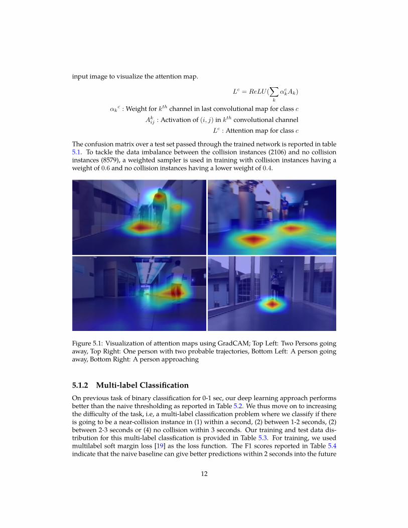
input image to visualize the attention map.

Lc = ReLU(∑k

αckAk)

αkc : Weight for kth channel in last convolutional map for class c

Akij : Activation of (i, j) in kth convolutional channel

Lc : Attention map for class c

The confusion matrix over a test set passed through the trained network is reported in table5.1. To tackle the data imbalance between the collision instances (2106) and no collisioninstances (8579), a weighted sampler is used in training with collision instances having aweight of 0.6 and no collision instances having a lower weight of 0.4.

Figure 5.1: Visualization of attention maps using GradCAM; Top Left: Two Persons goingaway, Top Right: One person with two probable trajectories, Bottom Left: A person goingaway, Bottom Right: A person approaching

5.1.2 Multi-label ClassificationOn previous task of binary classification for 0-1 sec, our deep learning approach performsbetter than the naive thresholding as reported in Table 5.2. We thus move on to increasingthe difficulty of the task, i.e, a multi-label classification problem where we classify if thereis going to be a near-collision instance in (1) within a second, (2) between 1-2 seconds, (2)between 2-3 seconds or (4) no collision within 3 seconds. Our training and test data dis-tribution for this multi-label classfication is provided in Table 5.3. For training, we usedmultilabel soft margin loss [19] as the loss function. The F1 scores reported in Table 5.4indicate that the naive baseline can give better predictions within 2 seconds into the future

12

Figure 5.2: Left: RGB Image, Right: Corresponding GradCAM

Table 5.1: Confusion Matrix from Binary Classification

Actualvalue

Prediction outcome

collision no collision

collision 634 36

no collision 53 2840

while the proposed multilabel deep neural network performs better for the latter classes,i.e., predictions in the range 2-3 seconds and no collision instances. One of the challengesof this multi-label formulation over the regression formulation is that we have to empiri-cally decide a threshold on the confidence score for each class to classify it as the positiveor negative label. The precision-recall curve or area under ROC curve [2] can be used toevaluate the performance of the trained model at different thresholds and then decide thebest threshold accordingly.

13

Table 5.2: Near-Collision Prediction formulated as Binary Classification: F1 Scores from ourapproach compared with a naive baseline

Method F1 ScoreNaive baseline (0.625Y ) 0.8488N-stream VGG (N = 4) 0.9344

Table 5.3: Class DistributionNear-Collision Time Training Data Test Data

0-1 s 4150 2871-2 s 2590 1852-3 s 2185 169

After 3 s 13049 507

5.2 Regression Experiments - Different temporal windowsas input

Overcoming the limitations of classification formulation, we move on to regression formu-lation which performed better as previously explained in chapter 4.

A single image can capture spatial information but no motion characteristics. Thus, wepropose to use a sequence of image frames as history. By feeding N image frames, weconsider a history of N−1

10 seconds. The temporal window of input frames was graduallyincreased from 2 frames (0.1 sec) to 9 frames (0.8 sec). We now describe our evaluationprocedure to decide the optimum temporal window as input on two different video net-work architectures. We further compare the performance with strong collision predictionbaselines. To quantify the performance, we measure the mean absolute error (MAE) for thepredictions on the test set of 1000 instances and the standard deviation in error. From Table5.6, it is empirically concluded to use a temporal window of 0.5 seconds, i.e, 6 frames formost accurate predictions.

We also report the error at different time-to-collision intervals in Table 5.5. It is easiest toforecast the collisions a second away and hence the error is least. In general, as forecastinghorizon increases it keeps on getting more difficult to forecast the exact time-to-collision.

5.3 Experimental comparison of architecturesWe show a comparison of the performance of multi-stream VGG model and baselines in-cluding state-of-the-art methods in Table 5.7.

1. Constant Baseline: On the training data of 12,620 samples, we compute the mean timeto near-collision denoted byE[ytrue] as a weak baseline. For each test input, we predictE[ytrue] which was found to be 2.23 seconds.

2. Tracking followed by constant velocity model: In dynamic environments, pedestrians areoften tracked using a stereo camera or LIDAR. By saving few previous locations (0.5-2seconds), a linear regression fit is used to predict the velocity vector of person [14],

14

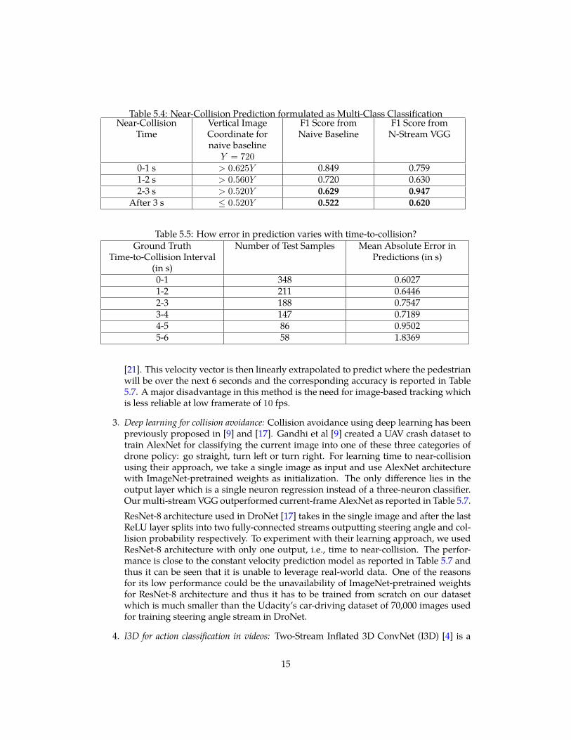
Table 5.4: Near-Collision Prediction formulated as Multi-Class ClassificationNear-Collision

TimeVertical ImageCoordinate fornaive baselineY = 720

F1 Score fromNaive Baseline

F1 Score fromN-Stream VGG

0-1 s > 0.625Y 0.849 0.7591-2 s > 0.560Y 0.720 0.6302-3 s > 0.520Y 0.629 0.947

After 3 s ≤ 0.520Y 0.522 0.620

Table 5.5: How error in prediction varies with time-to-collision?Ground Truth

Time-to-Collision Interval(in s)

Number of Test Samples Mean Absolute Error inPredictions (in s)

0-1 348 0.60271-2 211 0.64462-3 188 0.75473-4 147 0.71894-5 86 0.95025-6 58 1.8369

[21]. This velocity vector is then linearly extrapolated to predict where the pedestrianwill be over the next 6 seconds and the corresponding accuracy is reported in Table5.7. A major disadvantage in this method is the need for image-based tracking whichis less reliable at low framerate of 10 fps.

3. Deep learning for collision avoidance: Collision avoidance using deep learning has beenpreviously proposed in [9] and [17]. Gandhi et al [9] created a UAV crash dataset totrain AlexNet for classifying the current image into one of these three categories ofdrone policy: go straight, turn left or turn right. For learning time to near-collisionusing their approach, we take a single image as input and use AlexNet architecturewith ImageNet-pretrained weights as initialization. The only difference lies in theoutput layer which is a single neuron regression instead of a three-neuron classifier.Our multi-stream VGG outperformed current-frame AlexNet as reported in Table 5.7.ResNet-8 architecture used in DroNet [17] takes in the single image and after the lastReLU layer splits into two fully-connected streams outputting steering angle and col-lision probability respectively. To experiment with their learning approach, we usedResNet-8 architecture with only one output, i.e., time to near-collision. The perfor-mance is close to the constant velocity prediction model as reported in Table 5.7 andthus it can be seen that it is unable to leverage real-world data. One of the reasonsfor its low performance could be the unavailability of ImageNet-pretrained weightsfor ResNet-8 architecture and thus it has to be trained from scratch on our datasetwhich is much smaller than the Udacity’s car-driving dataset of 70,000 images usedfor training steering angle stream in DroNet.

4. I3D for action classification in videos: Two-Stream Inflated 3D ConvNet (I3D) [4] is a

15

Table 5.6: Distribution of absolute error (mean± std) on near-collision dataset using differ-ent number of input frames

Number of frames Multi-stream VGG I3D1 0.879 ± 0.762s 0.961 ± 0.707s2 0.828 ± 0.739s 0.879 ± 0.665s3 0.826 ± 0.647s 0.914 ± 0.659s4 0.866 ± 0.696s 0.811 ± 0.642s5 0.849 ± 0.734 0.845 ± 0.658s6 0.753 ± 0.687s 0.816 ± 0.663s7 0.757 ± 0.722s 0.848 ± 0.733s8 0.913 ± 0.732s 0.811 ± 0.647s9 0.817 ± 0.738s 0.855 ± 0.670s

Table 5.7: Distribution of absolute error (mean ± std) on regression task compared withdifferent baselines

Method Mean (in s) Std (in s)Constant baseline (E[ytrue]) 1.382 0.839

Tracking + Linear Model [14] 1.055 0.962DroNet [17] 1.099 0.842

Gandhi et al [9] 0.884 0.818Single Image VGG-16 0.879 0.762

I3D (4 frames) [4] 0.811 0.642Multi-stream VGG (6 frames) 0.753 0.687

strong baseline to learn a task from videos. All theN×N filters and pooling kernels inImageNet-pretrained Inception-V1 network [28] are inflated with an additional tem-poral dimension to become N × N × N . I3D has two streams - one trained on RGBinputs and other on optical flow inputs. To avoid adding the latency of optical flowcomputation for real-time collision forecasting, we only used the RGB stream of I3D.We fine-tuned the I3D architecture which was pre-trained on Kinetics Human ActionVideo dataset [4] on our near-collision dataset by sending N RGB frames as inputwhere N = {1, 2, . . . , 8, 9} as reported in Table 5.6. The outermost layer is modifiedfrom 400-neuron classifier to 1-neuron regressor. Since our N -frame input is smallerthan the original implementation on 64-frame input, we decreased the temporal strideof last max-pool layer from 2 to 1. While 6 input frames were found to be the best forproposed multi-stream VGG network, we experimented again with the optimal his-tory on I3D. The performance of I3D with varying number of input frames is reportedin Table 5.6. For N = 4, 6, 8, I3D is found to give the best results among 1-9 framesthough our multi-stream VGG prediction forN = 6 outperformed the I3D predictionin best case.

5.4 Qualitative EvaluationFrom the plots shown in Fig. 5.3 we can observe that the predictions given by multi-streamVGG on 6 frames give smoother output as compared to undesired fluctuations in I3D out-

16

Figure 5.3: Prediction of multi-stream VGG is smoother than I3D. The discontinuities herearise in the absence of pedestrians.

put. One of the plausible reason for I3D performing worse could be the average pool layerin I3D which averages the features over input frames. On the other hand, the proposednetwork preserves the temporal order of features of input frames which helps in under-standing the motion characteristics of people in scene. We also qualitatively show in Fig.5.4 the comparison of time to near-collision predicted by our method vs the ground truth.From Fig. 5.4, we can observe the cases when there are two humans in the scene and thenetwork’s predictions are based on the closest person approaching the platform.

17

Figure 5.4: Predictions on four different test videos

18

Chapter 6

Conclusion

We return to the question posed in introduction, ’Is it possible to predict the time to near-collision from a single camera?’. The answer is that the proposed model is able to leveragespatio-temporal cues for predicting the time to collision within 0.75 seconds on the testvideos. Also, we observed that the multi-stream network of shared weights performed thetask of collision forecasting better than I3D on the proposed dataset.

With regard to temporal window of input history, it is evident that using a sequenceof images has a considerable benefit over prediction from single frame only. Though thehistory of 0.5 seconds performed best, we do not observe a piecewise monotonic relationbetween input frames and error in prediction. This observation aligns with the performanceof constant velocity model where accuracy in prediction does not necessarily increase ordecrease with the temporal footprint of past trajectory.

We understand that the proposed model might not generalize well when there are largechanges in camera’s height, speed of the robot or structure of the scenes in comparison toprovided dataset. In the scenarios where assistive robot operates at walking speed and ina constrained domain like museums and airports, the proposed approach will be suitablefor predicting time to collision requiring only a low-cost monocular camera. InexpensiveRGB-D sensors like Kinect cannot be used for outdoor navigation while our approach canbe extended for outdoor use given training data.

19

Chapter 7

Future Work

In this work, the networks predicts a single real value as the time-to-collision and uses meansquared error loss for training. The current approach always outputs a real-valued estimateand there is no indicator on how confident or reliable is the prediction. In the future work,we can instead try to output two values - mean and variance in time-to-collision. The vari-ance can tell us the confidence in predicted value. Lower the variance, stronger is the peakof predicted mean. To train the output tuple of mean and variance, the negative of gaussianlog-likelihood loss can be minimized over the training data.

One of the scenarios where the proposed approach fails is when a person is moving inthe same direction as user. The pedestrian detector detects the person and so the image ispassed through the proposed multi-stream network. The network outputs an inaccurateestimate of time-to-collision as shown in Figure 7.1.

Figure 7.1: Inaccurate estimate of time-to-collision when a person is moving away from theassistive suitcase

One plausible way is to predict the variance term as mentioned above and hope thatthe variance will be large enough to not trust the prediction in such cases. As an alternatesolution, instead of passing the image first through the pedestrian detector, we can pass itthrough a binary classifier trained to classify if there is going to be a collision within thechosen time bound (here, 6 seconds) or not. If positive, we can then pass it through the

20

regressor network as proposed in this work to estimate the exact time-to-collision. Open-Pose [3], a real-time approach to detect the 2D pose of multiple people in an image includingfoot, torso, arms and face keypoints can possibly be leveraged to replace the object detectionbackbone, i.e, VGG-16 to enhance the prediction performance.

The prediction time bound in this work is chosen to be 6 seconds arbitrarily. Dependingon the application or the planner requirements, the time bound could be chosen accord-ingly. For a higher time bound, it would be challenging to learn the task within an accept-able error limit. The Table 7.1 reports how the error varies with prediction time horizon.

Table 7.1: Mean Absolute Error in Predicted Time varying with the Prediction Time HorizonPrediction Time Horizon (in seconds) Mean Absolute Error (in seconds)

5 0.5656 0.7537 0.903

21

Bibliography

[1] A. Alahi, K. Goel, V. Ramanathan, A. Robicquet, L. Fei-Fei, and S. Savarese. Social lstm: Humantrajectory prediction in crowded spaces. In Proceedings of the IEEE Conference on Computer Visionand Pattern Recognition, pages 961–971, 2016.

[2] A. P. Bradley. The use of the area under the roc curve in the evaluation of machine learningalgorithms. Pattern recognition, 30(7):1145–1159, 1997.

[3] Z. Cao, G. Hidalgo, T. Simon, S. Wei, and Y. Sheikh. Openpose: Realtime multi-person 2d poseestimation using part affinity fields. CoRR, abs/1812.08008, 2018.

[4] J. Carreira and A. Zisserman. Quo vadis, action recognition? A new model and the kineticsdataset. CoRR, abs/1705.07750, 2017.

[5] J. Deng, W. Dong, R. Socher, L.-J. Li, K. Li, and L. Fei-Fei. ImageNet: A Large-Scale HierarchicalImage Database. In CVPR09, 2009.

[6] A. Ess, B. Leibe, K. Schindler, and L. van Gool. Robust multiperson tracking from a mobileplatform. IEEE Transactions on Pattern Analysis and Machine Intelligence, 31(10):1831–1846, Oct2009.

[7] M. Everingham, L. Van Gool, C. K. Williams, J. Winn, and A. Zisserman. The pascal visual objectclasses (voc) challenge. International journal of computer vision, 88(2):303–338, 2010.

[8] C. Feichtenhofer, A. Pinz, and R. P. Wildes. Spatiotemporal residual networks for video actionrecognition. In NIPS, 2016.

[9] D. Gandhi, L. Pinto, and A. Gupta. Learning to fly by crashing. CoRR, abs/1704.05588, 2017.[10] A. Gupta, J. Johnson, L. Fei-Fei, S. Savarese, and A. Alahi. Social gan: Socially acceptable trajec-

tories with generative adversarial networks. 2018 IEEE/CVF Conference on Computer Vision andPattern Recognition, pages 2255–2264, 2018.

[11] K. He, X. Zhang, S. Ren, and J. Sun. Deep residual learning for image recognition. CoRR,abs/1512.03385, 2015.

[12] S. Hochreiter and J. Schmidhuber. Long short-term memory. Neural Comput., 9(8):1735–1780,November 1997.

[13] S. Kato, S. Tokunaga, Y. Maruyama, S. Maeda, M. Hirabayashi, Y. Kitsukawa, A. Monrroy,T. Ando, Y. Fujii, and T. Azumi. Autoware on board: Enabling autonomous vehicles with embed-ded systems. In Proceedings of the 9th ACM/IEEE International Conference on Cyber-Physical Systems,ICCPS ’18, 2018.

[14] S. Kayukawa, K. Higuchi, J. Guerreiro, S. Morishima, Y. Sato, K. Kitani, and C. Asakawa. Bbeep:A sonic collision avoidance system for blind travellers and nearby pedestrians. In Proc. ACM CHIConference on Human Factors in Computing Systems (CHI’19), CHI ’19, New York, NY, USA, May2019. ACM.

[15] A. Krizhevsky, I. Sutskever, and G. E. Hinton. Imagenet classification with deep convolutionalneural networks. In Advances in neural information processing systems, pages 1097–1105, 2012.

22

[16] A. Kushleyev and M. Likhachev. Time-bounded lattice for efficient planning in dynamic en-vironments. In 2009 IEEE International Conference on Robotics and Automation, pages 1662–1668,2009.

[17] A. Loquercio, A. I. Maqueda, C. R. del-Blanco, and D. Scaramuzza. Dronet: Learning to fly bydriving. IEEE Robotics and Automation Letters, 3(2):1088–1095, April 2018.

[18] J. Y.-H. Ng, M. J. Hausknecht, S. Vijayanarasimhan, O. Vinyals, R. Monga, and G. Toderici. Be-yond short snippets: Deep networks for video classification. 2015 IEEE Conference on ComputerVision and Pattern Recognition (CVPR), pages 4694–4702, 2015.

[19] A. Paszke, S. Gross, S. Chintala, G. Chanan, E. Yang, Z. DeVito, Z. Lin, A. Desmaison, L. Antiga,and A. Lerer. Automatic differentiation in pytorch. In NIPS-W, 2017.

[20] S. Pellegrini, A. Ess, K. Schindler, and L. V. Gool. You’ll never walk alone: Modeling socialbehavior for multi-target tracking. 2009 IEEE 12th International Conference on Computer Vision,pages 261–268, 2009.

[21] M. Phillips and M. Likhachev. Sipp: Safe interval path planning for dynamic environments. In2011 IEEE International Conference on Robotics and Automation, pages 5628–5635, May 2011.

[22] Z. Qiu, T. Yao, and T. Mei. Learning spatio-temporal representation with pseudo-3d residualnetworks. 2017 IEEE International Conference on Computer Vision (ICCV), pages 5534–5542, 2017.

[23] S. Ren, K. He, R. Girshick, and J. Sun. Faster r-cnn: Towards real-time object detection withregion proposal networks. In Proceedings of the 28th International Conference on Neural InformationProcessing Systems - Volume 1, NIPS’15, pages 91–99, Cambridge, MA, USA, 2015. MIT Press.

[24] A. Sadeghian, V. Kosaraju, A. Gupta, S. Savarese, and A. Alahi. Trajnet: Towards a benchmarkfor human trajectory prediction. arXiv preprint, 2018.

[25] R. R. Selvaraju, M. Cogswell, A. Das, R. Vedantam, D. Parikh, and D. Batra. Grad-cam: Visualexplanations from deep networks via gradient-based localization. In Proceedings of the IEEE In-ternational Conference on Computer Vision, pages 618–626, 2017.

[26] K. Simonyan and A. Zisserman. Two-stream convolutional networks for action recognition invideos. In Proceedings of the 27th International Conference on Neural Information Processing Systems- Volume 1, NIPS’14, pages 568–576, Cambridge, MA, USA, 2014. MIT Press.

[27] K. Simonyan and A. Zisserman. Very deep convolutional networks for large-scale image recog-nition. CoRR, abs/1409.1556, 2014.

[28] C. Szegedy, W. Liu, Y. Jia, P. Sermanet, S. E. Reed, D. Anguelov, D. Erhan, V. Vanhoucke, andA. Rabinovich. Going deeper with convolutions. CoRR, abs/1409.4842, 2014.

[29] D. Tran, L. Bourdev, R. Fergus, L. Torresani, and M. Paluri. Learning spatiotemporal features with3d convolutional networks. In Proceedings of the 2015 IEEE International Conference on ComputerVision (ICCV), ICCV ’15, 2015.

[30] A. Vemula, K. Muelling, and J. Oh. Path planning in dynamic environments with adaptive di-mensionality. In Ninth Annual Symposium on Combinatorial Search, 2016.

[31] A. Vemula, K. Muelling, and J. Oh. Social attention: Modeling attention in human crowds. InProceedings of the International Conference on Robotics and Automation (ICRA) 2018, May 2018.

[32] L. Zhou, Z. Li, and M. Kaess. Automatic extrinsic calibration of a camera and a 3d lidar usingline and plane correspondences. In IEEE/RSJ Intl. Conf. on Intelligent Robots and Systems, IROS,October 2018.

[33] B. D. Ziebart, N. Ratliff, G. Gallagher, C. Mertz, K. Peterson, J. A. Bagnell, M. Hebert, A. K. Dey,and S. Srinivasa. Planning-based prediction for pedestrians. In Intelligent Robots and Systems,2009. IROS 2009. IEEE/RSJ International Conference on, pages 3931–3936. IEEE, 2009.

23