reassessment of long-period constituents for tidal

Ocean Sci., 15, 1363–1379, 2019https://doi.org/10.5194/os-15-1363-2019© Author(s) 2019. This work is distributed underthe Creative Commons Attribution 4.0 License.

Reassessment of long-period constituents for tidal predictions alongthe German North Sea coast and its tidally influenced riversAndreas Boesch and Sylvin Müller-NavarraBundesamt für Seeschifffahrt und Hydrographie, Bernhard-Nocht-Straße 78, 20359 Hamburg, Germany

Correspondence: Andreas Boesch ([email protected])

Received: 12 June 2019 – Discussion started: 18 June 2019Revised: 9 September 2019 – Accepted: 12 September 2019 – Published: 18 October 2019

Abstract. The harmonic representation of inequalities(HRoI) is a procedure for tidal analysis and prediction thatcombines aspects of the non-harmonic and the harmonicmethod. With this technique, the deviations of heights andlunitidal intervals, especially of high and low waters, fromtheir respective mean values are represented by superpo-sitions of long-period tidal constituents. This article docu-ments the preparation of a constituents list for the opera-tional application of the harmonic representation of inequal-ities. Frequency analyses of observed heights and lunitidalintervals of high and low water from 111 tide gauges alongthe German North Sea coast and its tidally influenced rivershave been carried out using the generalized Lomb–Scargleperiodogram. One comprehensive list of partial tides is re-alized by combining the separate frequency analyses and byapplying subsequent improvements, e.g. through manual in-spections of long time series data. The new set of 39 partialtides largely confirms the previously used set with 43 par-tial tides. Nine constituents are added and 13 partial tides,mostly in the close neighbourhood of strong spectral com-ponents, are removed. The effect of these changes has beenstudied by comparing predictions with observations from 98tide gauges. Using the new set of constituents, the standarddeviations of the residuals are reduced on average by 2.41 %(times) and 2.30 % (heights) for the year 2016. The new setof constituents will be used for tidal analyses and predictionsstarting with the German tide tables for the year 2020.

1 Introduction

Tidal predictions for the German Bight are calculated at theFederal Maritime and Hydrographic Agency (Bundesamt fürSeeschifffahrt und Hydrographie, BSH) and are published inofficial tide tables each year. The preparation of tidal predic-tions has a long tradition at BSH and its predecessor institu-tions: the first tide tables by the German Imperial Admiraltywere issued for the year 1879.

Since 1954, a method named harmonic representation ofinequalities (HRoI) has been used at BSH to calculate tidalpredictions for tide gauge locations along the German NorthSea coast and its tidally influenced rivers (Horn, 1948, 1960;Müller-Navarra, 2013). This technique allows for analysingthe deviations of times and heights, especially at high andlow water, from their respective mean values. In contrast tothe widely used harmonic method (e.g. Parker, 2007, and ref-erences therein), the HRoI utilizes only long-period partialtides. This reduction in frequency space allows for a compu-tationally efficient way to calculate times and heights of highand low water. Other techniques for tidal analysis of high andlow waters have been described in Doodson (1951) and Fore-man and Henry (1979); these two methods additionally con-sider diurnal and semi-diurnal constituents. The HRoI hasproven to be especially useful for predicting semi-diurnaltides in shallow waters where the harmonic method wouldneed a large number (&60) of constituents or could even failto produce adequate results. The fundamentals of the HRoIare summarized in Sect. 2 for completeness.

An important aspect of tidal prediction is the selection ofrelevant partial tides (angular velocities, ω) to be includedin the underlying analysis of water level records. While it ispossible to determine these partial tides individually for eachsingle tidal analysis, it is desirable in an operational service

Published by Copernicus Publications on behalf of the European Geosciences Union.

1364 A. Boesch and S. Müller-Navarra: Reassessment of long-period constituents for tidal predictions

to have one comprehensive set of constituents that can beused for all tide gauges under investigation. Horn (1960) pre-sented a list of 44 angular velocities that were used with theHRoI. This selection of partial tides was probably utilizeduntil the year 1969 when the set was slightly modified (cf.Table 2 in Sect. 2). To our knowledge, no documentation ofthe methods and specific water level records that were usedto prepare these lists of angular velocities exists.

The objective of this work is to review the set of partialtides used with the HRoI by determining the most impor-tant long-period constituents for application in the GermanBight. Therefore, we perform a spectral analysis of waterlevel observations from 111 tide gauges. The available tidegauge data are presented in Sect. 3. The analysis of high-and low-water time series is described in Sect. 4. In Sect. 5,tidal predictions based on an existing list of partial tides andpredictions based on the new set are compared with observedwater levels. The article closes with a comparison of predic-tions made with the HRoI and the harmonic method for twosites (Sect. 6) and the conclusions (Sect. 7).

2 Harmonic representation of inequalities

The harmonic representation of inequalities (HRoI) is aderivative of the non-harmonic method by essentially trans-lating it into an analytical form. The non-harmonic methodhas been used for a long time, e.g. by Lubbock (1831) forthe analysis of tides in the port of London. With the non-harmonic method, the times of high and low waters are cal-culated by adding mean lunitidal intervals and correspond-ing inequalities to the times of lunar transits. Likewise, theheights of high and low waters are determined by adding cor-responding inequalities to the respective mean heights. Theinequalities are corrections for the relative positions of earth,moon and sun (e.g. semi-monthly, parallactic, declination).

The original implementation of the HRoI, as introduced byHorn (1948, 1960), can be used to calculate vertices of tidecurves, i.e. high-water time, high-water height, low-watertime and low-water height. In this form the method is tailoredto semi-diurnal tides. Müller-Navarra (2013) shows how theHRoI may be generalized to predict tidal heights at equidis-tant fractions of the mean lunar day. This generalization al-lows for the determination of the full tidal curve at a chosensampling interval. Here, we focus only on the application ofcalculating the times and heights of high and low waters.

According to Horn (1960), the HRoI combines the bestfrom the harmonic and the non-harmonic methods: the ana-lytical procedure of the first method and the principle of cal-culating isolated values directly, which a is characteristic ofthe second. The strength of the HRoI lies in the prediction oftimes and heights of high and low water when the full tidalcurve is considerably non-sinusoidal. This is frequently thecase in shallower waters, such as the German Bight, and inrivers. As the HRoI uses only observed times and/or heights

Table 1. The high and low waters are classified into four types(event index k).

k Description

1 high water assigned to upper transit2 low water assigned to upper transit3 high water assigned to lower transit4 low water assigned to lower transit

of high and/or low waters, the method can also be appliedwhen a record of the full tidal curve is not available (e.g. his-toric data) or when a tide gauge runs dry around low water(e.g. analysis of only high waters).

Let (tj ,hj ),j = 1, . . .,J, be a time series of length J ofhigh- and low-water heights hj recorded at times tj . Alltimes need to be given in UTC. The HRoI method is basedon the assumption that the variations in the individual heightsand lunitidal intervals around their respective mean valuescan be described by sums of harmonic functions. The luni-tidal interval is the time difference between the time tj andthe corresponding lunar transit at Greenwich. As a generalrule, the daily higher high water and the following low waterare assigned to the previous upper lunar transit, and the dailylower high water and the following low water are assigned tothe previous lower transit. For example, in the year 2018, themean lunitidal interval for high (low) water was determinedto be 9 h 4 min (16 h 5 min) for Borkum and 15 h 22 min (22 h32 min) for Hamburg. See Fig. 1 in Sect. 3 for the locationsof these two sites.

A convenient method to organize high and low waters ofsemi-diurnal tides is the lunar transit number nt (Müller-Navarra, 2009). It counts the number of upper lunar transits(unit symbol: tn) at the Greenwich meridian since the tran-sit on 31 December 1949, which has been arbitrarily set tont = 0 tn. A lower transit always has the same transit numberas the preceding upper transit. Each high and low water isuniquely identified by using the number, nt, of the assignedlunar transit and an additional event index, k, as defined inTable 1. The differentiation between upper and lower tran-sits allows for changes in the moon’s declination which al-ternately advance and retard times, and increase and decreasethe heights of successive tides (diurnal inequality).

A full tidal analysis with the HRoI comprises the inves-tigation of eight time series (heights and lunitidal intervalsof the four event types listed in Table 1). Each time series isdescribed by a model function, y, of the following form:

y(nt)= a0+

L∑l=1

[al cos(ωlnt)+ al+L sin(ωlnt)

]. (1)

Ocean Sci., 15, 1363–1379, 2019 www.ocean-sci.net/15/1363/2019/

A. Boesch and S. Müller-Navarra: Reassessment of long-period constituents for tidal predictions 1365

The parameters al, l = 0, . . .,2L are determined from aleast-squares fit, i.e.

χ2=

J∑j=0

(yj − yj

)2→min, (2)

where yj is the observed heights or lunitidal intervals. Theangular velocities ωl (◦ tn−1) are taken from a previously de-fined set of L partial tides. In Table 2, we list two sets ofpartial tides that have been used in the past at BSH and thenew set that is the result of this work.

All tidal constituents considered here have angular veloci-ties that are linear combinations of the rate of change of fourfundamental astronomical arguments: the mean longitudeof the moon (s), the mean longitude of the sun (h), themean longitude of the lunar perigee (p) and the negativeof the longitude of the moon’s ascending node (N ′). Thesecond to fifth columns in Table 2 give the respective linearcoefficients m. The two other arguments that one encountersusing the harmonic method can be effectively neglected:the coefficients for the rate of change of the mean lunartime and of the mean longitude of the solar perigee arealways equal to zero because only long-period constituentsneed to be considered and the time series are too short toresolve differences due to the variations in the solar perigee.The angular velocities in the sixth and seventh columnsare given in degrees per hour and in degrees per transitnumber (tn), respectively. The conversion between these twounits is 1◦ tn−1

·τ [ htn ] = 1◦ h−1 with the length of the mean

lunar day τ = 24.84120312 h tn−1. The angular velocitiesare calculated using the expressions for the fundamentalastronomical arguments as published by the InternationalEarth Rotation and Reference Systems Service (2010,Sect. 5.7). The alphabetical Doodson number is given inthe first column (Doodson, 1921; Simon, 2013). The eighthcolumn states the commonly used names (e.g. see the Inter-national Hydrographic Organization (IHO) Standard List ofTidal Constituents: https://www.iho.int/mtg_docs/com_wg/IHOTC/IHOTC_Misc/TWCWG_Constituent_list.pdf, lastaccess: 4 October 2019). An “x” mark in one of the last threecolumns indicates whether the angular velocity is includedin the respective constituents list for usage with the HRoI.

3 Tide gauge data

The tide gauges at the German coast and in rivers are oper-ated by different federal and state authorities. These agen-cies provide BSH with quality-checked water level recordsof high and low waters (times and heights). Table A1 in theAppendix lists 137 German tide gauges which deliver waterlevel observations on a regular basis and for which tidal pre-dictions were published in BSH tide tables (Gezeitentafeln)or the tide calendar (Gezeitenkalender) for the year 2018(Bundesamt für Seeschifffahrt und Hydrographie, 2017a, b).

Figure 1. The locations of all tide gauges in the German Bight fromTable A1. Some of the tide gauges mentioned in the text are high-lighted: Borkum, Fischerbalje (B); Emden, Große Seeschleuse (E);Cuxhaven, Steubenhöft (C); and Hamburg, St. Pauli (H).

For the analysis presented in Sect. 4, all data until the year2015 that were systematically archived in electronic format the BSH tidal information service are considered (as ofAugust 2018). The data periods are given in the fourth andfifth columns in Table A1 and cover 22–27 years for mostgauges. Much longer time series were readily available fortide gauges at Cuxhaven (BSH gauge number 506P) andHamburg (508P) for which data since the year 1901 are used.We are aware that the tidal regime can change over such along time but include all available data in the analysis to max-imize the achievable spectral resolution.

Only tide gauges with more than 19 years of data are in-cluded in order to cover the period of rotation of the lunarnode (18.6 years) in the frequency analysis. In addition, weuse only tide gauges where more than 60 % of high and lowwaters are recorded during the gauge’s data period. This cri-terion excludes gauges for which no low-water observationsare available. The 111 gauges that fulfil these two criteriaare marked in the column labelled “Used for analysis” in Ta-ble A1. The locations of all tide gauges are shown on the mapin Fig. 1.

4 Analysis of high-water and low-water time series

The following analysis is applied to the water level recordsof all 111 tide gauges that are marked in the seventh columnof Table A1 in the Appendix.

www.ocean-sci.net/15/1363/2019/ Ocean Sci., 15, 1363–1379, 2019

https://www.iho.int/mtg_docs/com_wg/IHOTC/IHOTC_Misc/TWCWG_Constituent_list.pdf

https://www.iho.int/mtg_docs/com_wg/IHOTC/IHOTC_Misc/TWCWG_Constituent_list.pdf


Table 2. Sets of angular velocities that have been used with the HRoI. See Sect. 2 for a description of the columns.

Doodson ms mh mp mN ′ ω (◦ h−1) ω (◦ tn−1) Name Set 1a Set 2b This work

ZZZZAZ 0 0 0 1 0.0022064 0.0548098 x x xZZZAZZ 0 0 1 0 0.0046418 0.1153082 xZZZBZZ 0 0 2 0 0.0092836 0.2306165 xZZAYZZ 0 1 −1 0 0.0364268 0.9048862 xZZAZZZ 0 1 0 0 0.0410686 1.0201944 Sa x x xZZBXZZ 0 2 −2 0 0.0728537 1.8097724 x x xZZBZZZ 0 2 0 0 0.0821373 2.0403886 Ssa x x xZAXZZZ 1 −2 0 0 0.4668792 11.5978420 x x xZAXAZZ 1 −2 1 0 0.4715211 11.7131503 MSm x x xZAYXZZ 1 −1 −2 0 0.4986643 12.3874200 xZAYZZZ 1 −1 0 0 0.5079479 12.6180365 xZAYAAZ 1 −1 1 1 0.5147961 12.7881545 xZAZYYZ 1 0 −1 −1 0.5421683 13.4681129 x xZAZYZZ 1 0 −1 0 0.5443747 13.5229227 Mm x x xZAZZYZ 1 0 0 −1 0.5468101 13.5834211 x xZAZZZZ 1 0 0 0 0.5490165 13.6382309 x x xZAZZAZ 1 0 0 1 0.5512229 13.6930407 x x xZAZAZZ 1 0 1 0 0.5536583 13.7535391 xZABYZZ 1 2 −1 0 0.6265120 15.5633115 x xZABBAZ 1 2 2 1 0.6426438 15.9640460 xZBVBZZ 2 −4 2 0 0.9430421 23.4263005 xZBWZZZ 2 −3 0 0 0.9748271 24.2158785 x x xZBXZYZ 2 −2 0 −1 1.0136894 25.1812631 x x xZBXZZZ 2 −2 0 0 1.0158958 25.2360729 MSf x x xZBXZAZ 2 −2 0 1 1.0181022 25.2908827 x xZBXAZZ 2 −2 1 0 1.0205376 25.3513811 x xZBYZZZ 2 −1 0 0 1.0569644 26.2562673 xZBZXZZ 2 0 −2 0 1.0887494 27.0458453 x x xZBZYZZ 2 0 −1 0 1.0933912 27.1611535 x x xZBZZYZ 2 0 0 −1 1.0958266 27.2216520 x xZBZZZZ 2 0 0 0 1.0980330 27.2764618 Mf x x xZBZZAZ 2 0 0 1 1.1002394 27.3312716 x x xZCVAZZ 3 −4 1 0 1.4874168 36.9492232 Sν2 x x xZCWYZZ 3 −3 −1 0 1.5192018 37.7388011 x xZCXYYZ 3 −2 −1 −1 1.5580641 38.7041858 x xZCXYZZ 3 −2 −1 0 1.5602705 38.7589956 SN x x xZCXYAZ 3 −2 −1 1 1.5624769 38.8138054 x xZCXZZZ 3 −2 0 0 1.5649123 38.8743038 x x xZCXAZZ 3 −2 1 0 1.5695541 38.9896120 MStm x x xZCZWZZ 3 0 −3 0 1.6331241 40.5687675 xZCZYZZ 3 0 −1 0 1.6424077 40.7993844 Mfm x x xZDUZZZ 4 −5 0 0 1.9907229 49.4519514 x x xZDVZZZ 4 −4 0 0 2.0317915 50.4721458 2SM x x xZDXXZZ 4 −2 −2 0 2.1046452 52.2819182 x xZDXZZZ 4 −2 0 0 2.1139288 52.5125347 MSqm x x xZDXZAZ 4 −2 0 1 2.1161352 52.5673444 xZDZZZZ 4 0 0 0 2.1960661 54.5529235 x x xZETAZZ 5 −6 1 0 2.5033126 62.1852961 x x xZEVYZZ 5 −4 −1 0 2.5761662 63.9950685 2SMN x x xZEVZZZ 5 −4 0 0 2.5808080 64.1103767 xZEVAZZ 5 −1 1 0 2.5854499 64.2256849 xZEXYZZ 5 −2 −1 0 2.6583035 66.0354573 x xZFTZZZ 6 −6 0 0 3.0476873 75.7082187 x x xZFVZZZ 6 −4 0 0 3.1298246 77.7486076 x x xZHRZZZ 8 −8 0 0 4.0635830 100.9442917 x x x

Number of partial tides in set of constituents 44 43 39

a Set 1 was probably used until the year 1969, see also Table 3 in Horn (1960). b Set 2 was probably used from 1970 until 2019, see alsoappendix E in Goffinet (2000), Table 5 in Müller-Navarra (2013) includes ω = 23.4263005◦ tn−1 but this angular velocity has never been includedin calculations for BSH tide tables or the tide calendars.



4.1 Data preparation

Data preparation includes the assignment of lunar transitnumbers, nt, and the calculation of lunitidal intervals as de-scribed in Sect. 2 for each record of high or low water. Thelunar transit times are calculated following the algorithm byMeeus (1998, Chap. 15) with the modification of direct cal-culation of lunar coordinates using the periodic terms givenin the work by Chapront-Touzé and Chapront (1991).

The observed water levels include extreme events, such asstorm surges. These events are not representative for the tidalbehaviour at the site of a tide gauge and are removed fromthe data set. We apply a 3σ clipping separately for the eighttime series analysed with the HRoI (see Sect. 2). Only thosedata points for which the height and the lunitidal interval arewithin the range of 3 times the respective standard deviationare used in the analysis.

4.2 Frequency analysis

The observed heights and lunitidal intervals (y) can be under-stood as being functions of the assigned transit number (nt).We calculate periodograms for the heights and tidal intervalsusing the corresponding frequency scale per transit number.

The occurrences of high and low waters are irregularlyspaced in time. Additionally, there are many longer datagaps which cannot be interpolated. This excludes the fastFourier transform (FFT) as a spectral analysis technique. In-stead, we use the generalized Lomb–Scargle periodogram asdefined by Zechmeister and Kürster (2009), including theirnormalization if not mentioned otherwise. The frequencyscale covers the range from 0.0001 to 2 tn−1 with an in-terval of 0.01999 tn−1 (100 000 points in the periodogram).This corresponds to approximately 0.0057–114.5916◦ tn−1

or 0.0002–4.6130◦ h−1. The upper limit corresponds to twicethe mean sampling interval (Nyquist criterion).

Artefacts from spectral leakage pose a major problemwhen identifying peaks in a periodogram. They arise fromthe finite length of the time series. This effect can be reducedby applying an apodization function, i.e. multiplying the datawith a suitable window function, that smoothly brings therecorded values to zero at the beginning and the end of thesampled time series (e.g. Press et al., 1992; Prabhu, 2014).We apply a Hanning window to the data, which gives a goodcompromise between reducing side lobes and preserving thespectral resolution.

For each tide gauge, periodograms are calculated for theeight time series that are analysed with the HRoI. In Figs. 2aand 3a, we show periodograms of the lunitidal intervals andheights (of high waters assigned to an upper transit, event in-dex k = 1) for the tide gauge Cuxhaven. Cuxhaven (togetherwith Hamburg) provides by far the longest time series that isused in the analysis (cf. Table A1). In these figures, the verti-cal axis is normalized to the strongest peak and the horizon-tal axis is converted to degrees per transit number for better

Figure 2. (a) Normalized periodogram of the lunitidal intervals ofhigh waters (assigned to upper lunar transits) for the tide gaugeCuxhaven. Notice the upper part of the logarithmic scale is trun-cated at 0.1 for better visibility of weak lines. (b) Zoomed-in viewof the region with the spectral line corresponding to half a tropicalmonth (Mf) at 27.2764618◦ tn−1. The longer time series for Cux-haven leads to narrower spectral lines (solid blue curve) comparedto Emden (dashed green line).

comparison with Table 2. The periodogram for the lunitidalintervals reveals many more strong spectral lines above thenoise level as compared to the periodogram for the heights.A frequency-dependent noise level can clearly be seen inFig. 3a (noise level increases towards lower angular veloc-ities). Figs. 2b and 3b show a small extract of the respectiveupper periodograms. Additionally, data for tide gauge Emdenare included for illustration of the differences in spectral linewidth. The time series from Emden is about 4 times shorterthan the one from Cuxhaven. This leads to broader spectrallines in the periodogram and it can be expected that someweaker lines are unresolvable.



Figure 3. (a) Normalized periodogram of the heights of high wa-ters (assigned to upper lunar transits) for the tide gauge Cuxhaven.Notice the logarithmic scale. (b) Zoomed-in view of the regionwith the spectral line corresponding to half a tropical month (Mf)at 27.2764618◦ tn−1. The longer time series for Cuxhaven leadsto narrower spectral lines (solid blue curve) compared to Emden(dashed green line).

4.3 Identifying relevant partial tides

We aim to find all local maxima in a periodogram that areabove a noise threshold. This threshold is calculated in a two-step process that is described in the following.

In the first step, the strongest spectral lines are removedfrom the periodogram. The values above the 99.5th percentileare removed from the data set and a histogram is calculatedfrom the remaining values p (100 bins with central valuesxbin). The histogram shows an exponential trend from a largenumber of data points with low periodogram values to a fewpoints that fall into the bins at the upper end. An exponentialcurve, ybin = a · exp(−xbin/b), is fitted to the histogram withfit parameters a and b. The process of removing data pointsabove the 99.5th percentile from the periodogram is repeated

Figure 4. Determination of the noise threshold for the tidal interval(high water, upper transit) at tide gauge Borkum, Fischerbalje. Thestrongest lines are removed from the periodogram (grey vs. greenlines; first step as described in Sect. 4.3) and an exponential function(dashed red curve) is fitted to selected points (blue; second step asdescribed in Sect. 4.3). The noise threshold (thick red line) is shiftedup by 1 standard deviation.

until the ratio max(p)/b falls below the value of 30. Thisvalue is based on experience.

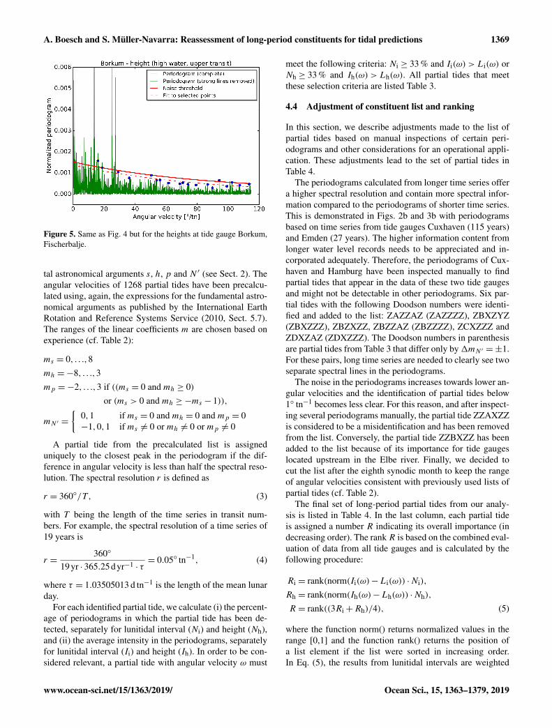
In the second step, the noise threshold is determined usinga set of remaining points in the periodogram that representa continuum above the noise level. The result is illustratedin Figs. 4 and 5 for lunitidal intervals and heights at the tidegauge Borkum. For this procedure, the periodogram is splitinto 25 sections with the same number of data points. Thedata point at the 99.5th percentile is selected in each sectionand an exponential function is fitted to these 25 points. Thefit is repeated after a 1σ clipping. The noise threshold corre-sponds to the resulting exponential function plus 1 standarddeviation (solid red line in Figs. 4 and 5).

In preparation for the following combined evaluation ofthe results from all tide gauges, the noise threshold functionsfrom the different periodograms are averaged; this is sepa-rately for lunitidal intervals (Li) and heights (Lh):

Li(ω)= 0.0004816 · exp(−0.0101045 tn/◦ ·ω),Lh(ω)= 0.0024472 · exp(−0.0149899 tn/◦ ·ω).

These two functions represent mean lower-intensity bound-aries for the selection of significant peaks. The expressionsLi andLh are unitless, due to the normalization of the Lomb–Scargle periodogram (Zechmeister and Kürster, 2009).

In addition to the intensity of the local maxima, the num-ber of their occurrences in the different periodograms andtheir assignment to the partial tides determine their inclusioninto the list of constituents for the HRoI. The local maximamust match the theoretically expected partial tides that havewell-known angular velocities computable from the linearcombinations of the rate of change of the four fundamen-



Figure 5. Same as Fig. 4 but for the heights at tide gauge Borkum,Fischerbalje.

tal astronomical arguments s, h, p and N ′ (see Sect. 2). Theangular velocities of 1268 partial tides have been precalcu-lated using, again, the expressions for the fundamental astro-nomical arguments as published by the International EarthRotation and Reference Systems Service (2010, Sect. 5.7).The ranges of the linear coefficients m are chosen based onexperience (cf. Table 2):

ms = 0, . . .,8mh =−8, . . .,3mp =−2, . . .,3 if ((ms = 0 and mh ≥ 0)

or (ms > 0 and mh ≥−ms − 1)),

mN ′ =

{0,1 if ms = 0 and mh = 0 and mp = 0−1,0,1 if ms 6= 0 or mh 6= 0 or mp 6= 0

A partial tide from the precalculated list is assigneduniquely to the closest peak in the periodogram if the dif-ference in angular velocity is less than half the spectral reso-lution. The spectral resolution r is defined as

r = 360◦/T , (3)

with T being the length of the time series in transit num-bers. For example, the spectral resolution of a time series of19 years is

r =360◦

19yr · 365.25d yr−1 · τ= 0.05◦ tn−1, (4)

where τ = 1.03505013 d tn−1 is the length of the mean lunarday.

For each identified partial tide, we calculate (i) the percent-age of periodograms in which the partial tide has been de-tected, separately for lunitidal interval (Ni) and height (Nh),and (ii) the average intensity in the periodograms, separatelyfor lunitidal interval (Ii) and height (Ih). In order to be con-sidered relevant, a partial tide with angular velocity ω must

meet the following criteria: Ni ≥ 33 % and Ii(ω) > Li(ω) orNh ≥ 33 % and Ih(ω) > Lh(ω). All partial tides that meetthese selection criteria are listed Table 3.

4.4 Adjustment of constituent list and ranking

In this section, we describe adjustments made to the list ofpartial tides based on manual inspections of certain peri-odograms and other considerations for an operational appli-cation. These adjustments lead to the set of partial tides inTable 4.

The periodograms calculated from longer time series offera higher spectral resolution and contain more spectral infor-mation compared to the periodograms of shorter time series.This is demonstrated in Figs. 2b and 3b with periodogramsbased on time series from tide gauges Cuxhaven (115 years)and Emden (27 years). The higher information content fromlonger water level records needs to be appreciated and in-corporated adequately. Therefore, the periodograms of Cux-haven and Hamburg have been inspected manually to findpartial tides that appear in the data of these two tide gaugesand might not be detectable in other periodograms. Six par-tial tides with the following Doodson numbers were identi-fied and added to the list: ZAZZAZ (ZAZZZZ), ZBXZYZ(ZBXZZZ), ZBZXZZ, ZBZZAZ (ZBZZZZ), ZCXZZZ andZDXZAZ (ZDXZZZ). The Doodson numbers in parenthesisare partial tides from Table 3 that differ only by1mN ′ =±1.For these pairs, long time series are needed to clearly see twoseparate spectral lines in the periodograms.

The noise in the periodograms increases towards lower an-gular velocities and the identification of partial tides below1◦ tn−1 becomes less clear. For this reason, and after inspect-ing several periodograms manually, the partial tide ZZAXZZis considered to be a misidentification and has been removedfrom the list. Conversely, the partial tide ZZBXZZ has beenadded to the list because of its importance for tide gaugeslocated upstream in the Elbe river. Finally, we decided tocut the list after the eighth synodic month to keep the rangeof angular velocities consistent with previously used lists ofpartial tides (cf. Table 2).

The final set of long-period partial tides from our analy-sis is listed in Table 4. In the last column, each partial tideis assigned a number R indicating its overall importance (indecreasing order). The rankR is based on the combined eval-uation of data from all tide gauges and is calculated by thefollowing procedure:

Ri = rank(norm(Ii(ω)−Li(ω)) ·Ni),

Rh = rank(norm(Ih(ω)−Lh(ω)) ·Nh),

R = rank((3Ri+Rh)/4), (5)

where the function norm() returns normalized values in therange [0,1] and the function rank() returns the position ofa list element if the list were sorted in increasing order.In Eq. (5), the results from lunitidal intervals are weighted



Table 3. The most important partial tides that were identified in the periodograms, based on the combined evaluation of data from all tidegauges. See Sect. 4.3 for information on selection criteria and Ii, Ih, Ni and Nh.

Doodson ω (◦ tn−1) Ii (–) Ih (–) Ni (%) Nh(%)

ZZZZAZ 0.0548098 0.0086 0.0102 78 45ZZZBZZ 0.2306165 0.0019 0.0085 29 47ZZAXZZ 0.7895780 0.0009 0.0088 16 34ZZAZZZ 1.0201944 0.0070 0.0367 85 84ZZBZZZ 2.0403886 0.0013 0.0068 26 56

ZAXZZZ 11.5978420 0.0009 0.0034 69 35ZAXAZZ 11.7131503 0.0234 0.0024 100 10ZAYXZZ 12.3874200 0.0006 0.0031 2 65ZAYZZZ 12.6180365 0.0007 0.0042 34 21ZAYAAZ 12.7881545 0.0005 0.0031 1 45

ZAZYZZ 13.5229227 0.0112 0.0119 99 90ZAZZZZ 13.6382309 0.0105 0.0297 97 87ZAZAZZ 13.7535391 0.0006 0.0016 63 2ZABBAZ 15.9640460 0.0010 0.0032 1 70ZBWZZZ 24.2158785 0.0029 0.0081 83 7

ZBXZZZ 25.2360729 0.4550 0.0706 100 92ZBYZZZ 26.2562673 0.0034 0.0079 55 9ZBZYZZ 27.1611535 0.0008 0.0021 43 29ZBZZZZ 27.2764618 0.0382 0.0070 100 85ZCVAZZ 36.9492232 0.0037 0.0013 99 25

ZCXYZZ 38.7589956 0.0009 0.0014 89 9ZCXAZZ 38.9896120 0.0010 0.0004 96 0ZCZYZZ 40.7993844 0.0008 0.0000 93 0ZDUZZZ 49.4519514 0.0004 0.0000 38 0ZDVZZZ 50.4721458 0.0196 0.0025 100 73

ZDXZZZ 52.5125347 0.0059 0.0015 99 15ZDZZZZ 54.5529235 0.0003 0.0003 43 0ZETAZZ 62.1852961 0.0006 0.0000 93 0ZEVYZZ 63.9950685 0.0003 0.0001 61 0ZEVAZZ 64.2256849 0.0004 0.0000 78 0

ZFTZZZ 75.7082187 0.0014 0.0003 98 2ZFVZZZ 77.7486076 0.0010 0.0003 97 5ZHRZZZ 100.9442917 0.0002 0.0000 36 0ZHTZZZ 102.9846805 0.0002 0.0002 37 0

stronger because the noise level is lower in the respective pe-riodograms.

The rank R can be used to select a sub-list of partial tideswhen performing a tidal analysis of water levels with lessthan 18.6 years of data. This is important because not all par-tial tides can be resolved against each other for shorter timeseries. The minimum difference in angular velocity is givenby the resolution criterion (Eq. 3). Figure 6 illustrates the re-solvable partial tides as a function of the length of the datarecord. Note that the high-ranked partial tide representing thetropical month which occurs at R = 4 in the list cannot be in-cluded for time series shorter than about 9 years. For a tidalanalysis of time series shorter than 9 years, it is therefore of-ten better to perform a reference analysis: 19 years of data are

used from a different tide gauge with a similar tidal behaviour(e.g. similar course of the semi-monthly inequality) and theresults are translated to the original gauge by applying the re-spective differences in the mean lunitidal intervals and meanheights. This way, nodal corrections can be avoided whichcome with their own assumptions and approximations (e.g.Godin, 1986; Amin, 1987).

5 Comparison of predictions with observations: twodifferent lists of constituents for the HRoI

For verification of the new constituent list, tidal predictionsbased on an existing list of partial tides and based on the



Table 4. The modified and adopted new list of long-period partialtides. The rank R indicates the importance of a partial tide for tidalanalysis, based on the combined evaluation of data from all tidegauges.

Doodson ω (◦ tn−1) Description, name R

ZZZZAZ 0.0548098 lunar nodal precession 6ZZZBZZ 0.2306165 half lunar apsidal precession 13ZZAZZZ 1.0201944 tropical year, Sa 7ZZBXZZ 1.8097724 31ZZBZZZ 2.0403886 half tropical year, Ssa 17

ZAXZZZ 11.5978420 14ZAXAZZ 11.7131503 MSm 8ZAYXZZ 12.3874200 34ZAYZZZ 12.6180365 19ZAYAAZ 12.7881545 39

ZAZYZZ 13.5229227 anomalistic month, Mm 3ZAZZZZ 13.6382309 tropical month 4ZAZZAZ 13.6930407 38ZAZAZZ 13.7535391 21ZABBAZ 15.9640460 36

ZBWZZZ 24.2158785 11ZBXZYZ 25.1812631 35ZBXZZZ 25.2360729 half synodic month, MSf 1ZBYZZZ 26.2562673 12ZBZXZZ 27.0458453 33

ZBZYZZ 27.1611535 15ZBZZZZ 27.2764618 half tropical month, Mf 2ZBZZAZ 27.3312716 27ZCVAZZ 36.9492232 Sν2 10ZCXYZZ 38.7589956 SN 16

ZCXZZZ 38.8743038 24ZCXAZZ 38.9896120 MStm 22ZCZYZZ 40.7993844 Mfm 23ZDUZZZ 49.4519514 29ZDVZZZ 50.4721458 fourth synodic month, 2SM 5

ZDXZZZ 52.5125347 MSqm 9ZDXZAZ 52.5673444 37ZDZZZZ 54.5529235 30ZETAZZ 62.1852961 25ZEVYZZ 63.9950685 2SMN 28

ZEVAZZ 64.2256849 26ZFTZZZ 75.7082187 sixth synodic month 20ZFVZZZ 77.7486076 18ZHRZZZ 100.9442917 eighth synodic month 32

Figure 6. The partial tides (identified by their rank R from Ta-ble 4) that can be resolved as a function of the (minimum) length ofthe time series. If two partial tides cannot be resolved against eachother, the one with the lower rank is dropped. Note the logarithmictime axis from 0.2 to 20 years. The numbers at the top are the countsof partial tides.

new set are compared with observations. The predictions aremade for the year 2016 and are compared with tide gaugeobservations from the same year.

5.1 Tidal analysis and prediction

We calculate tidal predictions (times and heights of high andlow waters) with the HRoI using (i) the 43 partial tides fromSet 2 in Table 2 and (ii) the 39 partial tides derived from ouranalysis. The data and software are otherwise identical. Thepredictions are based on amplitudes am (see Eq. 1) that aredetermined from a tidal analysis of water level records from1995 to 2013 (19 years). Data are only used from tide gaugesthat have delivered enough observations in this time period toinclude all partial tides in the analysis. Additionally, the tidegauges must have delivered observations for the year 2016.The 98 tide gauges that fulfil these criteria are marked in thecolumn “Used for verif.” in Table A1. All tide gauge data areprepared as described in Sect. 4.1, including the removal ofextreme events from the observations that are used for com-parison. The analysis is applied in two iterations with a 3σclipping in-between.

5.2 Evaluation of residuals

In this section, we present results from the analysis of theresiduals in the following order: the distributions of resid-uals for the tide gauge Cuxhaven, the means and standarddeviations for some major ports, the changes in the standarddeviations for all tide gauges, and the changes in the remain-



Figure 7. Histograms of the residuals for tide gauge Cuxhaven andyear 2016. The different colours indicate predictions based on thedifferent sets of partial tides (red: predictions with 43 partial tides;yellow: predictions with 39 partial tides). (a) Time differences witha bin width of 4 min. (b) Height differences with a bin width of0.04 m.

ing frequencies. The residuals are the differences betweenthe observed and the predicted vertices (times and heights ofhigh and low waters) with the same assigned transit numberand event index k.

Figure 7 shows histograms of the residuals for the tidegauge Cuxhaven. The panels on the left and on the right dis-play histograms for the times and heights, respectively. Eachpanel contains one histogram for the tidal prediction with 43partial tides (red) and one histogram for the tidal predictionwith 39 partial tides (yellow). Using the new set of partialtides, the standard deviation of the residuals decreases from9.6 to 9.0 min for the times and from 0.28 to 0.27 m for theheights.

In the same way as for Cuxhaven, residuals are calculatedfor the data of all 98 tide gauges included in the verifica-tion. The mean values, µ, and standard deviations, σ , of theresiduals for 11 major ports are summarized in Table 5 forthe times and in Table 6 for the heights. Based on the re-sults from all tide gauges, the average standard deviation ofthe residuals is 13.2 min or 0.28 m, respectively, using the setof 39 tidal constituents. In most cases, the new set of partialtides gives small improvements in µ and σ .

The percentage changes, 1σ , in the standard deviationsare presented in the histograms in Fig. 8 (times) and Fig. 9(heights) for all 98 tide gauges. The percentage change iscalculated in the following way:

1σ [%] = 100% ·σ39 p.t.− σ43 p.t.

σ43 p.t., (6)

where σ39 p.t. and σ43 p.t. are the standard deviations of theresiduals using the predictions with 39 partial tides (p.t.) and43 partial tides, respectively. The average reductions of thestandard deviations are 2.41 % (times) and 2.30 % (heights).The two tide gauges with the largest improvements in this

Table 5. Residuals of predicted and observed times of high and lowwater: mean µ and standard deviation σ in minutes.

Gauge Gauge 43 partial tides 39 partial tides

number name µ σ µ σ

101P Borkum −2.7 11.2 −2.1 11.0103P Bremerhaven −6.4 10.4 −4.6 10.1111P Norderney 1.5 10.9 0.7 10.6502P Bremen −7.3 10.8 −5.5 10.5505P Büsum 3.4 17.5 4.6 17.4506P Cuxhaven −0.1 9.6 1.0 9.0507P Emden −9.2 13.8 −8.2 13.3508P Hamburg −10.1 10.4 −7.7 10.3509A Helgoland −2.4 7.8 −2.6 7.7510P Husum −5.1 12.0 −4.3 11.7512P Wilhelmshaven −3.2 10.0 −2.7 9.6

Table 6. Residuals of predicted and observed heights of high andlow water: mean µ and standard deviation σ in metres.

Gauge Gauge 43 partial tides 39 partial tides

number name µ σ µ σ

101P Borkum 0.05 0.24 0.03 0.24103P Bremerhaven 0.06 0.28 0.04 0.28111P Norderney 0.03 0.25 −0.01 0.24502P Bremen 0.01 0.27 −0.01 0.26505P Büsum 0.04 0.29 0.01 0.28506P Cuxhaven 0.05 0.28 0.04 0.27507P Emden −0.01 0.28 −0.02 0.27508P Hamburg −0.08 0.33 −0.12 0.31509A Helgoland 0.03 0.25 0.02 0.24510P Husum 0.02 0.29 0.00 0.28512P Wilhelmshaven 0.05 0.27 0.03 0.27

study, both with regard to times and heights, are Holmer Siel(BSH gauge number 649B) at the North Frisian coast andBremervörde (687P) in the river Oste. Further tide gaugeswith improved standard deviations are located all around thearea of investigation. Regarding the times (Fig. 8), the fourtide gauges with increased standard deviations are Wester-land (620P) and Hörnum (624P), located on the North Frisianisland of Sylt, and Dove-Elbe (727P) and Bunthaus (729P),located upstream of the river Elbe. Regarding the heights(Fig. 9), the five tide gauges with the largest positive changesare also located upstream in the Elbe, namely Geesthacht(732D), Altengamme (732A), Zollenspieker (731P), Ilmenau(730A) and Fahrenholz (730C). The water levels in this partof the Elbe are partly influenced by river discharge, whichcan lead to deviations from the tidal predictions.

The change in constituents has an influence on the remain-ing periodicities in the residuals. Periodograms are calcu-lated for the two sets of residuals (times and heights) foreach tide gauge. The 98 periodograms of each type are aver-



Figure 8. Histogram of the change in the standard deviation of theresiduals of high- and low-water times for all 98 tide gauges.

Figure 9. Histogram of the change in the standard deviation of theresiduals of high- and low-water heights for all 98 tide gauges.

aged. The resulting mean periodograms are shown in Figs. 10and 11. In both figures, the strongest peaks are located atvery low angular velocities (.1◦ tn−1). As mentioned before,the unambiguous identification of partial tides at these peri-ods is difficult and consequently no major improvements areachieved in reducing the (average) residual periodicities inthis range. Four further strong peaks are visible in both fig-ures at about 15, 25, 52 and 64◦ tn−1 for the prediction with43 partial tides. These peaks are clearly reduced with the newpredictions (39 partial tides).

6 Comparison of predictions with observations: theHRoI and the harmonic method

The harmonic method is the most widely used technique fortidal predictions. The following comparison of predictionscalculated with the HRoI and with the harmonic methods will

Figure 10. Mean periodogram of residual high- and low-watertimes for all tide gauges used in the verification. The differentcolours indicate predictions based on the different sets of partialtides (red: predictions with 43 partial tides; yellow: predictions with39 partial tides)

Figure 11. Same as Fig. 10 but for the high- and low-water heights.

demonstrate the respective capabilities. The comparison isdone for the two tide gauges at Cuxhaven, Steubenhöft, andHamburg, St. Pauli. The first site is located at the mouth ofthe river Elbe, flowing into the North Sea, while the second isabout 100 km upstream in the river Elbe. The predictions arecompared with tide gauge observations from the year 2016.

6.1 Tidal analysis and prediction

The predictions with the HRoI (39 partial tides) are the sameas in Sect. 5. The harmonic analysis is based on continuousobservations from the years 1996 to 2014 at 10 min intervals.The harmonic constituents (amplitudes H and phases g) andthe constant vertical offset, Z0, are determined from a least-



Figure 12. Observations and two predictions for the tide gauge Cux-haven, Steubenhöft. The first 10 d of June 2016 are shown.

squares fit with the following model function:

yharm = Z0+

L∑l=1

[Hl · cos(Vl(t0)+ωl t − gl)

]. (7)

We use the 68 partial tides (with angular velocities ωl)from Foreman (1977). These are also the default constituentsin the MATLAB packages t_tide and UTide (Pawlowiczet al., 2002; Codiga, 2011), which have become widely ac-cepted standard implementations of the harmonic method.Since the data records exceed 18.6 years, we add the par-tial tide with the angular velocity of the lunar node and omitnodal corrections. This gives a total of L= 69 constituents.The time t is referenced to the midpoint t0 of the time seriesand the astronomical argument Vl(t0) is calculated for eachpartial tide using the expressions for the fundamental astro-nomical arguments as published by the International EarthRotation and Reference Systems Service (2010, Sect. 5.7).The analysis is applied in two iterations with a 3σ clippingin-between to remove outliers in the observations.

We show in Figs. 12 and 13 the predictions and obser-vations for Cuxhaven and Hamburg, respectively. Only 10 din June 2016 are shown from the complete time series forbetter visibility of the individual high and low waters. Thetwo curves in each figure are the observed water levels (darkblue) and the harmonic prediction (light green). The highand low waters are marked separately for observations (redcircles), vertices determined from the harmonic prediction(green squares) and predictions made with the HRoI (yellowtriangles).

6.2 Evaluation of residuals

As in Sect. 5, the residuals are the differences between theobserved and the predicted vertices (times and heights ofhigh and low waters) with the same assigned transit number

Figure 13. Observations and two predictions for the tide gaugeHamburg, St. Pauli. The first 10 d of June 2016 are shown.

Table 7. Residuals of predicted and observed times and heights ofhigh and low water: mean µ and standard deviation σ .

Times (min)

Gauge name HRoI (39 p.t.) Harmonic pred.

µ σ µ σ

Cuxhaven 1.0 9.0 12.0 12.9Hamburg −7.7 10.3 11.8 15.1

Heights (m)

Gauge name HRoI (39 p.t.) Harmonic pred.

µ σ µ σ

Cuxhaven 0.03 0.27 0.05 0.29Hamburg −0.11 0.31 −0.10 0.37

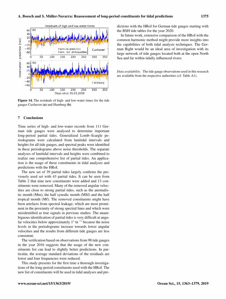
and event index k. We calculate the means and the standarddeviations of the residuals regarding times and heights. Theresults are shown in Table 7. The differences for the heightsare within a few centimetres. For the times, the standard de-viations are approximately 4–5 min larger in the case of theharmonic method. The residuals for the times are also shownin Fig. 14, where the curves for the harmonic method (blue)suggest that long-period periodicities could be present in theresiduals which are not covered by the predictions. Based onthe calculated parameters, the deviations of the harmonic pre-diction from the observations (and also from the predictionmade with the HRoI) are larger for Hamburg as comparedto Cuxhaven. This supports the assumptions that the applica-tion of the HRoI is especially useful for tide gauge locationsin rivers.



Figure 14. The residuals of high- and low-water times for the tidegauges Cuxhaven (a) and Hamburg (b).

7 Conclusions

Time series of high- and low-water records from 111 Ger-man tide gauges were analysed to determine importantlong-period partial tides. Generalized Lomb–Scargle pe-riodograms were calculated from lunitidal intervals andheights for all tide gauges, and spectral peaks were identifiedin these periodograms above noise thresholds. The separateanalyses of lunitidal intervals and heights were combined torealize one comprehensive list of partial tides. An applica-tion is the usage of these constituents in tidal analyses andpredictions with the HRoI.

The new set of 39 partial tides largely confirms the pre-viously used set with 43 partial tides. It can be seen fromTable 2 that nine new constituents were added and 13 con-stituents were removed. Many of the removed angular veloc-ities are close to strong partial tides, such as the anomalis-tic month (Mm), the half synodic month (MSf) and the halftropical month (Mf). The removed constituents might havebeen artefacts from spectral leakage, which are most promi-nent in the proximity of strong spectral lines and which weremisidentified as true signals in previous studies. The unam-biguous identification of partial tides is very difficult at angu-lar velocities below approximately 1◦ tn−1 because the noiselevels in the periodograms increase towards lower angularvelocities and the results from different tide gauges are lessconsistent.

The verification based on observations from 98 tide gaugesin the year 2016 suggests that the usage of the new con-stituents list can lead to slightly better predictions. In par-ticular, the average standard deviations of the residuals arelower and four frequencies were reduced.

This study presents for the first time a thorough investiga-tions of the long-period constituents used with the HRoI. Thenew list of constituents will be used in tidal analyses and pre-

dictions with the HRoI for German tide gauges starting withthe BSH tide tables for the year 2020.

In future work, extensive comparison of the HRoI with thecommon harmonic method might provide more insights intothe capabilities of both tidal analysis techniques. The Ger-man Bight would be an ideal area of investigation with itslarge network of tide gauges located both at the open NorthSea and far within tidally influenced rivers.

Data availability. The tide gauge observations used in this researchare available from the respective authorities (cf. Table A1).



Appendix A: Table of tide gauges

Table A1. 137 German tide gauges which deliver water level observations on a regular basis and for which tidal predictions were published inBSH tide tables (Gezeitentafeln) or the tide calendar (Gezeitenkalender) for the year 2018. The data from the tide gauges are observed timesand heights of high and low water. The tide gauges are operated by different federal and state agencies which provide tide gauge records toBSH. Abbreviations in the third column correspond to the following agencies: E: Emden Waterways and Shipping Authority (Wasserstraßen-und Schifffahrtsamt Emden, WSA Emden), BH: WSA Bremerhaven, B: WSA Bremen, C: WSA Cuxhaven, T: WSA Tönning, HPA: HamburgPort Authority, W: WSA Wilhelmshaven, HU: Landesbetrieb für Küstenschutz, Nationalpark und Meeresschutz Schleswig-Holstein (LKN-SH Husum), H: WSA Hamburg, L: WSA Lauenburg, N: Niedersächsischer Landesbetrieb für Wasserwirtschaft, Küsten- und Naturschutz(NLWKN), and M: WSA Meppen.

BSH gauge Gauge name Auth. Data period Data period Completeness Used for Used fornumber (start–end date) (year) of data (%) analysis verif.

101P Borkum, Fischerbalje E 02.01.1963–31.12.2015 53.0 62 x x103P Bremerhaven, Alter Leuchtturm BH 01.11.1965–31.12.2015 50.2 62 x x111P Norderney, Riffgat E 01.01.1964–31.12.2015 52.0 67 x x502P Bremen, Oslebshausen B 01.01.1950–31.12.2015 66.0 99 x x504A Brunsbüttel, Mole 1 C 01.08.2010–31.12.2015 5.4 95505P Büsum T 01.01.1963–31.12.2015 53.0 63 x x506P Cuxhaven, Steubenhöft C 01.01.1901–31.12.2015 115.0 99 x x507P Emden, Große Seeschleuse E 01.01.1989–31.12.2015 27.0 99 x x508P Hamburg, St. Pauli HPA 01.01.1901–31.12.2015 115.0 100 x x509A Helgoland, Binnenhafen T 01.01.1989–31.12.2015 27.0 99 x x510P Husum T 01.01.1989–31.12.2015 27.0 98 x x512P Wilhelmshaven, Alter Vorhafen W 01.01.1973–31.12.2015 43.0 98 x x613C Hojer, Schleuse HU 01.01.1999–31.12.2015 17.0 100617P List, Hafen T 01.01.1986–31.12.2015 30.0 98 x x618P Munkmarsch HU 16.01.1989–31.12.2015 27.0 49620P Westerland HU 01.01.1986–31.12.2015 30.0 94 x x622P Amrum Odde HU 17.04.1996–07.12.2015 19.6 40623A Rantumdamm HU 08.01.1996–31.12.2015 20.0 89 x624P Hörnum, Hafen T 01.01.1989–31.12.2015 27.0 99 x x628A Osterley HU 09.04.1997–11.11.2015 18.6 40629B Föhrer Ley Nord HU 27.04.1994–11.11.2015 21.5 46631P Amrum, Hafen (Wittdün) T 01.01.1989–31.12.2015 27.0 96 x632P Föhr, Wyk HU 01.01.1989–31.12.2015 27.0 100 x x635P Dagebüll T 01.01.1989–31.12.2015 27.0 99 x x636F Hooge, Anleger HU 01.01.1989–31.12.2015 27.0 93 x x637A Strand, Hamburger Hallig HU 02.05.1989–31.12.2015 26.7 79 x637P Gröde, Anleger HU 01.01.1989–31.12.2015 27.0 48638P Schlüttsiel HU 01.01.1989–31.12.2015 27.0 96 x x642C Rummelloch, West HU 14.06.1994–08.12.2015 21.5 47645P Süderoogsand HU 23.03.1993–20.11.2015 22.7 62 x647A Pellworm, Anleger T 01.03.1996–31.12.2015 19.8 88 x649B Holmer Siel HU 01.01.1994–31.12.2015 22.0 89 x x649P Nordstrand, Strucklahnungshörn HU 01.01.1989–31.12.2015 27.0 96 x x653P Südfall, Fahrwasserkante HU 25.03.1993–02.12.2015 22.7 67 x655D Tümlauer Hafen HU 24.09.2001–31.12.2013 12.3 93



Table A1. Continued.


658B Linnenplate HU 11.04.2001–05.12.2013 12.7 62664P Eidersperrwerk, AP T 01.01.1989–31.12.2014 26.0 97 x666P Blauort HU 12.01.1989–31.12.2015 27.0 82 x x667B Meldorf – Sperrwerk, AP HU 04.01.1994–31.12.2015 22.0 71 x669P Deichsiel HU 01.01.1989–31.12.2013 25.0 96 x673P Trischen, West HU 18.03.1989–25.11.2015 26.7 61 x675C Mittelplate HU 01.01.1992–25.11.2015 23.9 55675P Friedrichskoog, Hafen HU 01.01.1989–31.12.2015 27.0 100 x x676P Zehnerloch C 01.01.1989–14.11.2015 26.9 98 x x677C Scharhörnriff, Bake A C 01.01.2001–31.12.2015 15.0 96677P Scharhörn, Bake C C 01.01.1989–31.12.2015 27.0 98 x x678W Neuwerk HPA 01.01.1994–31.12.2015 22.0 46681A Neufeld, Hafen HU 01.01.1994–31.12.2015 22.0 78 x x681P Otterndorf C 01.01.1989–31.12.2015 27.0 79 x682P Osteriff C 01.01.1989–31.12.2015 27.0 89 x683P Belum, Oste C 01.01.1989–31.12.2015 27.0 96 x x685P Hechthausen, Oste C 01.01.1989–31.12.2015 27.0 95 x x687P Bremervörde, Oste C 01.01.1989–31.12.2015 27.0 94 x x688P Brokdorf H 01.01.1989–31.12.2015 27.0 98 x x690P Stör – Sperrwerk, AP HU 01.01.2000–31.12.2015 16.0 87691R Kasenort, Stör HU 01.01.1989–31.12.2015 27.0 99 x x692P Itzehoe, Stör H 01.01.1989–31.12.2015 27.0 97 x693P Breitenberg, Stör H 01.01.2000–31.12.2015 16.0 95695P Glückstadt H 01.01.1989–31.12.2015 27.0 95 x x697P Krautsand H 01.01.1989–31.12.2015 27.0 89 x x698P Kollmar (Kamperreihe) H 01.01.1989–31.12.2015 27.0 98 x x700R Krückau – Sperrwerk, BP H 01.01.2000–31.12.2015 16.0 89703P Grauerort H 01.01.1989–31.12.2015 27.0 98 x x704R Pinnau – Sperrwerk, BP H 01.01.2000–31.12.2015 16.0 93706P Uetersen, Pinnau H 01.01.1989–31.12.2015 27.0 92 x x709P Stadersand, Schwinge H 01.01.1989–31.12.2015 27.0 98 x x711P Hetlingen H 01.01.1989–31.12.2015 27.0 94 x x712P Lühort, Lühe H 01.01.1989–31.12.2015 27.0 97 x x714P Schulau H 01.01.1989–31.12.2015 27.0 97 x x715P Blankenese, Unterfeuer HPA 01.01.1989–31.12.2015 27.0 98 x x717P Cranz, Este – Sperrwerk, AP H 01.01.1989–31.12.2015 27.0 83 x x718P Buxtehude, Este H 01.01.1989–31.12.2015 27.0 86 x x720P Seemannshöft HPA 01.01.1989–31.12.2015 27.0 100 x x724P Harburg, Schleuse HPA 01.01.1989–31.12.2015 27.0 100 x x727P Dove – Elbe, Einfahrt HPA 01.01.1989–31.12.2015 27.0 99 x x729P Bunthaus HPA 01.01.1989–31.12.2015 27.0 100 x x730A Ilmenau – Sperrwerk, AP L 01.01.1989–31.12.2015 27.0 98 x x730C Fahrenholz, Ilmenau L 01.01.1989–31.12.2015 27.0 93 x x730P Over L 01.01.1989–31.12.2015 27.0 98 x x731P Zollenspieker L 01.01.1989–31.12.2015 27.0 98 x x732A Altengamme L 01.01.1989–31.12.2015 27.0 96 x x732D Geesthacht, Wehr UP L 01.01.1989–31.12.2015 27.0 98 x x734P Alte Weser, Leuchtturm BH 01.01.1989–31.12.2015 27.0 99 x x735A Spieka Neufeld N 01.01.1989–31.12.2015 27.0 50735B Wremertief N 01.01.1994–31.12.2015 22.0 38737P Dwarsgat, Unterfeuer BH 01.01.1989–31.12.2015 27.0 99 x x737S Robbensüdsteert BH 01.01.1989–31.12.2015 27.0 96 x x



Table A1. Continued.


738P Fedderwardersiel N 01.01.1989–31.12.2015 27.0 49741A Nordenham, Unterfeuer BH 01.01.1989–31.12.2015 27.0 99 x x741B Rechtenfleth BH 01.01.1993–31.12.2015 23.0 99 x x743P Brake B 01.01.1989–31.12.2015 27.0 97 x x744A Elsfleth Ohrt B 01.01.1989–31.12.2015 27.0 96 x x744P Elsfleth B 01.01.1975–31.12.2015 41.0 80 x x745P Huntebrück, Hunte B 01.01.1989–31.12.2015 27.0 98 x x746P Hollersiel, Hunte B 01.01.1989–31.12.2015 27.0 98 x x747P Reithörne, Hunte B 01.01.1989–31.12.2015 27.0 98 x x748P Oldenburg – Drielake, Hunte B 01.01.1989–31.12.2015 27.0 97 x x749P Farge B 01.01.1989–31.12.2015 27.0 99 x x750A Wasserhorst, Lesum B 01.01.1989–31.12.2015 27.0 90 x x750B Ritterhude, Hamme B 01.01.1989–31.12.2015 27.0 91 x x750C Niederblockland, Wümme B 01.01.1989–31.12.2015 27.0 91 x x750D Borgfeld, Wümme B 01.01.1989–31.12.2015 27.0 90 x x750P Vegesack B 01.01.1975–31.12.2015 41.0 80 x x751P Bremen, Wilhelm–Kaisen–Brück B 01.01.1989–31.12.2015 27.0 99 x x752P Bremen, Weserwehr B 01.01.1989–31.12.2015 27.0 98 x x754P Wangerooge, Langes Riff, (Nord) W 01.01.1976–31.12.2015 40.0 71 x x756P Wangerooge, Ost W 01.05.1976–31.12.2015 39.7 58 x760P Mellumplate, Leuchtturm W 01.01.1989–31.12.2015 27.0 99 x x761P Schillig W 01.01.1989–31.12.2015 27.0 92 x x764B Hooksielplate W 01.01.1989–31.12.2015 27.0 93 x x766P Voslapp W 01.01.1989–31.12.2015 27.0 95 x x769P Wilhelmshaven, Ölpier W 01.01.1989–31.12.2015 27.0 97 x x770P Wilhelmshaven, Neuer Vorhafen W 01.01.1989–31.12.2015 27.0 97 x x773P Arngast, Leuchtturm W 15.05.2001–31.12.2015 14.6 88776P Vareler Schleuse N 01.01.1989–31.12.2015 27.0 49777P Wangerooge, West W 01.01.1976–31.12.2015 40.0 73 x x778P Harlesiel N 01.01.1989–31.12.2015 27.0 57779P Spiekeroog E 01.01.1989–31.12.2015 27.0 98 x x781P Langeoog E 01.01.1989–31.12.2015 27.0 98 x x782P Bensersiel N 01.01.1989–31.12.2015 27.0 100 x x796C Leybucht, Leyhörn N 01.01.1992–31.12.2015 24.0 100 x x798P Borkum, Südstrand E 02.01.1989–31.12.2015 27.0 95 x x799G Dukegat E 01.01.1989–31.12.2015 27.0 95 x x799P Emshörn E 01.01.1989–31.12.2015 27.0 99 x x802P Knock E 01.01.1989–31.12.2015 27.0 99 x x803P Pogum, Ems E 01.01.1989–31.12.2015 27.0 98 x x805P Terborg, Meßstelle, Ems E 01.01.1989–31.12.2015 27.0 98 x x806P Leerort, Ems E 01.01.1989–31.12.2015 27.0 97 x x808A Leda – Sperrwerk, Unterpegel E 01.01.1989–31.12.2015 27.0 98 x x810A Nortmoor, Altarm Jümme N 01.01.2000–31.12.2015 16.0 85810B Detern, Jümme N 01.01.2000–31.12.2015 16.0 86810P Westringaburg, Leda N 01.01.1989–31.12.2015 27.0 84 x x812P Dreyschloot, Leda E 01.01.1989–31.12.2015 27.0 89 x x813P Weener, Ems E 01.01.1989–31.12.2015 27.0 98 x x814B Rhede, Ems M 01.01.1989–31.12.2015 27.0 94 x x814P Papenburg, Ems E 01.01.1989–31.12.2015 27.0 98 x x816P Herbrum, Hafendamm, Ems M 01.01.1989–01.11.2015 26.8 82 x

Number of tide gauges 111 98



Author contributions. Both authors designed the study and dis-cussed the results. AB analysed the data and prepared the articlewith input from SMN.

Competing interests. The authors declare that they have no conflictof interest.

Special issue statement. This article is part of the specialissue “Developments in the science and history of tides(OS/ACP/HGSS/NPG/SE inter-journal SI)”. It is not associ-ated with a conference.

Review statement. This paper was edited by Philip Woodworth andreviewed by three anonymous referees.

References

Amin, M.: A method for approximating the nodal modulations ofreal tides, Int. Hydrogr. Rev., 64, 103–113, 1987.

Bundesamt für Seeschifffahrt und Hydrographie: Gezeitentafeln2018, Europäische Gewässer, BSH, Hamburg and Rostock,2017a.

Bundesamt für Seeschifffahrt und Hydrographie: Gezeitenkalender2018, Hoch- und Niedrigwasserzeiten für die Deutsche Buchtund deren Flussgebiete, BSH, Hamburg and Rostock, 2017b.

Chapront-Touzé, M. and Chapront, J.: Lunar Tables and Programmsfrom 4000 B.C. to A.D. 8000, Willmann-Bell, Richmond, Vir-ginia, 1991.

Codiga, D. L.: Unified Tidal Analysis and Prediction Using theUTide Matlab Functions, Technical report 2011-01, GraduateSchool of Oceanography, University of Rhode Island, 2011.

Doodson, A. T.: The Harmonic Development of the Tide-Generating Potential, P. R. Soc. London A, 100, 305–329,https://doi.org/10.1098/rspa.1921.0088, 1921.

Doodson, A. T.: The analysis of high and low waters, Int. Hydrogr.Rev., 28, 13–77, 1951.

Foreman, M. G. G.: Manual for Tidal Heights Analysis and Predic-tion, Pacific Marine Science Report, 77-10, 1977.

Foreman, M. G. G. and Henry, R. F.: Tidal Analysis Based on Highand Low Water Observations, Pacific Marine Science Report, 79-15, 1979.

Godin, G.: The use of nodal corrections in the calculation of har-monic constants, Int. Hydrogr. Rev., 63, 143–162, 1986.

Goffinet, P.: Qualitätssteigerung der Seevermessung und Navigationdurch neuartige Beschickungsverfahren, Phd thesis, UniversitätHannover, 2000.

Horn, W.: Über die Darstellung der Gezeiten als Funktion der Zeit,Deutsche Hydrographische Zeitschrift, 1, 124–140, 1948.

Horn, W.: Some recent approaches to tidal problems, Int. Hydr.Rev., 37, 65–84, 1960.

International Earth Rotation and Reference Systems Service: IERSConventions (2010), Verlag des Bundesamts für Kartographieund Geodäsie, Frankfurt am Main, 2010.

Lubbock, J. W.: On the tides in the port of London, P. T. Roy. Soc.London, 121, 349–415, https://doi.org/10.1098/rstl.1831.0022,1831.

Meeus, J.: Astronomical Algorithms, Willmann-Bell, Richmond,Virginia, 1998.

Müller-Navarra, S.: Zur automatischen Scheitelpunktbestimmunggemessener Tidekurven in der Deutschen Bucht, Hydrologie undWasserbewirtschaftung, 53, 380–388, 2009.

Müller-Navarra, S.: Gezeitenvorausberechnungen mit der Har-monischen Darstellung der Ungleichheiten (On Tidal Predictionsby Means of Harmonic Representation of Inequalities), Berichtedes Bundesamtes für Seeschifffahrt und Hydrographie, Hamburgand Rostock, 50, 2013.

Parker, B. B.: Tidal Analysis and Prediction, U.S. Department ofCommerce, NOAA Special Publication NOS CO-OPS 3, 2007.

Pawlowicz, R., Beardsley, B., and Lentz, S.: Classical tidalharmonic analysis including error estimates in MAT-LAB using T_TIDE, Comput. Geosci., 28, 929–937,https://doi.org/10.1016/S0098-3004(02)00013-4, 2002.

Prabhu, K. M. M.: Window Functions and Their Applications inSignal Processing, CRC Press, Boca Raton, 2014.

Press, W. H., Teukolsky, S. A., Vetterling, W. T., and Flannery, B. P.:Numerical Recipes in FORTRAN, Cambridge University Press,Cambridge, 1992.

Simon, B.: Coastal Tides, Institut océanographique, Paris, 2013.Zechmeister, M. and Kürster, M.: The generalised Lomb-Scargle

periodogram. A new formalism for the floating mean andKeplerian periodograms, Astron. Astrophys., 496, 577–584,https://doi.org/10.1051/0004-6361:200811296, 2009.


https://doi.org/10.1098/rspa.1921.0088

https://doi.org/10.1098/rstl.1831.0022

https://doi.org/10.1016/S0098-3004(02)00013-4

https://doi.org/10.1051/0004-6361:200811296

reassessment of long-period constituents for tidal

Documents