S

AD-A241 104 i-,

REDUCED INTERFERENCE TIME-FREQUENCYDISTRIBUTIONS: APPLICATIONS TO

ACOUSTIC TRANSIENTS

William J. WilliamsProject Director

Electrical Engineering and Computer ScienceSystems Division

University of Michigan

Final Report forONR Contract

N00014-89-J- 1723

-ISjRUTIfN sr Nr A

Appro- '- PUL releaseDi," t .on Untnitsd

91-11804l liil l~l !lll Jlli/lll !l/t l//llti 9-

Abstract

A new conceptualization of time-frequency (t-f) energy distributions isdiscussed in this paper. Many new t-f distrbutions with desirable propertiesmay now be designed with relative ease by arproaching the problem in terms ofthe ambiguity plane representation of the kernel. Careful attention to the designprinciples yields kernels which result in high resolution t-f distributions with aconsiderable reduction of the sometimes troublesome cross terms observedwhen using other distributions such as the Wigner Distribution (WD) Whenthese new t-f distributions are applied to some common signals, fascinating newdetails emerge. Examples are provided for joint sounds and marine mammalsounds.

Background

Signals of practical interest often do not conform to the requirements ofrealistic application of Fourier principles. The approach works best when thesignal of interest is composed of a number of discrete frequency components sothat time is not a specific issue, (e.g. a constant frequency sinusoid) or somewhatparadoxically, when the signal exists for a very short time so that its time ofoccurrence is considered to be known (e.g. an impulse function). Much of whatwe are taught implies that signals that can not be satisfactorily represented inthese ways are somehow suspect and must be forced into the mold orabandoned.

It has been quite difficult to hanale nonstationary signals such as chirpssatisfactorily using conceptualizations based on stationarity. The spectrogramrepresents an attempt to apply the Fourier Transform for a short-time analysiswindow, within which it is hoped that the signal behaves reasonably accordingto the requirements of stationarity. By moving the analysis window along thesignal, one hopes to track and capture the variations of the signal spectrum as afunction of timt. The spectrogram has many useful properties including a welldeveloped general theory. The spectrogram often presents serious difficultieswhen used to analyze rapidly varying signals, however. If the analysis windowis made short enough to capture rapid changes in the signal it becomesimpossible to resolve frequency components of the signai which are close infrequency during the analysis window duration.

The WD has many important and interesting properties. It provides a highresolution representation in time and in frequency for a non stationary signalsuch as a chirp. In addition, the WD has the important property of satisfying thetime and frequency marginals. However, its energy distribution is not non-

Williams-RID 1

negative and it often possesses severe cross terms, or interference terms,between components in different t-f regions, potentially leading to confusion andmisinterpretation.

Both the spectrogram and the WD are members of Cohen's Class ofDistributions. Cohen has provided a consistent set of definitions for a desirableset of t-f distributions which has been of great value in guiding and clarifyingefforts in this area of research. Among the desirable properties are the absenceof negativity of the energy values (the spectrogram has this property, the WDdoes not) and the property of proper time and frequency marginals (the WD hasit, the spectrogram does not). A recent comprehensive review by Cohen providesan excellent overview of time-frequency distributions and recent results'.

Any member of Cohen's Class of distributions can be obtained by combininga kernel with a i.-stantaneous autocorrelation. In the ambiguity plane. Some ofthe relationships are shown below.

A(v, -t)g(v, r)

R(t, )" t SlyV)" l",(v.f)

Usual coputation W(L) f t Gmf)

followed by F

W(t,tf)= fx(t+,cl2)x*(t--tl2)e-j2%fT dt (Wigner Dist.) M1t

A(v,,t)= fx(t+,rl2)x*(t--rl2)e'j2xfxdr (Sym. Ambig. Fen) (2)

t All Integrals are over the entire real axis

Williams-RID 2

Many investigators have considered the WD to be the basic t-f distribution.Its principal faults, non-negativity and the cross terms have been considered tobe facts of life which can only be dealt with by performing additionalcomputations. Recent developments in our group have convinced us that thereare many t-f distributions with properties nearly as desirable as the WD, butwith considerably reduced interference terms. Figure 1 illustrates the effect ofthree choices of kernels, the WD kernel (Figure Ia.), the spectrogram kernel(Figure lb.) and a new kernel 2 designed to shape the generalized ambiguityfunction so as to reduce cross terms (Figure lc.). The kernel for this distributionis of the form

gr (vt) = exp(- v2 t 2 /0) (3)where a is the parameter to control the amount of interference suppression. Weshall discuss distributions in this paper which have kernels with similarcharacteristics.

Reduced Interference Distributions

Figure ld. is the ambiguity function of two different frequency sinewavesegments occuring at different times. The time domain representation of thesetwo signals is shown in front of the t-f distribution obtained assuming thekernels immediately above them were multiplied by the ambiguity function ofthe two signals. Computation was in the discrete form. Figure le. shows theresult obtained using the WD kernel, Figure If. shows the result obtained using apossible spectrogram kernel (two-dimensional gaussian) and Figure lg. showsthe results using gr(v,t) . One can see that there are strong interference termsbetween the two signals in the WD representation. The spectrogram has no crossterms, but the t-f representation is not a faithful representation of the timeduration and frequency spread of the two signals. Figure 1g shows a quitefaithful representation of the two signals, however. The time and frequencyresolution is nearly the same as the WD, but the interference terms are notvisible.

A descriptive name has been given to distributions whose kernels possessthe four characteristics which lead to the much reduced interference terms. Thename Reduced Interference Distribution or RID has been proposed". The reasonthat the RID approach is successful can easily be seen by looking at the.-. ,guiry function in Figure Id. The desired components of the ambiguityfunction fall near the crigi,. Tb., interference terms are far from the origin 4 .The WD kernel includes them with equal weight along with the desired terms

Williams-RID 3

because of its unity value. The RID kernel suppresses these interference terms,however, and retains the desired terms.

Figure 2 represents a more ambitious comparison of the WD, spectrogramand RID kernel results. Figures 2a. 2b and 2c show the results for the WD, thespectrogram kernel and the RID. The signal is composed of a chirp plus FMsignal. The WD represents the signals well, but strong interference terms areobserved between the two signals 5 . The spectrogram represents the chirp fairlywell, but the FM signal is very poorly represented, however. The RID result isessentially as good as the WD result for the desired parts of the t-f distribution,but with hardly any interference terms, in sharp contrast to the WD.

The required properties of RID, a list of desirable properties and somedistribution comparisons are shovn in Tables I and 2 the Essential ReducedInterference Distribution Requirements.

Applications

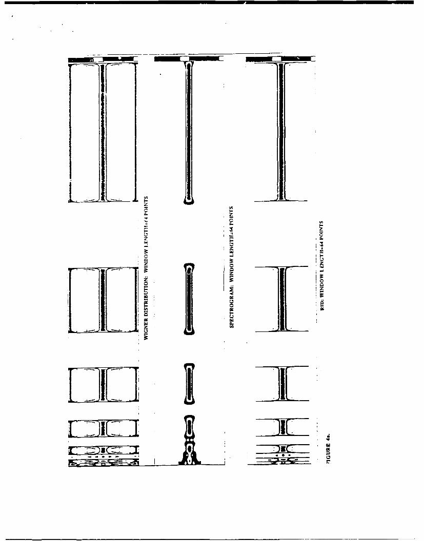
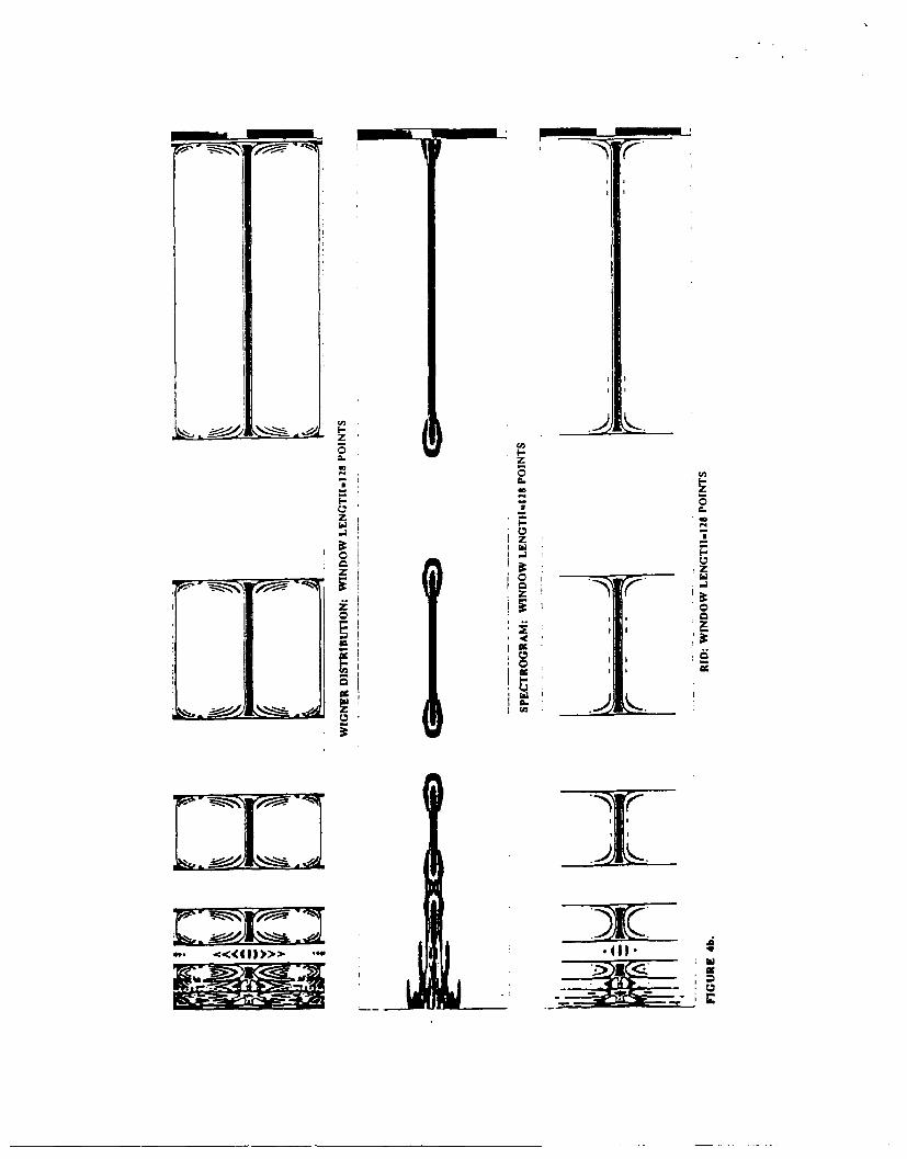
Some comparisons of RID with spectrograms and WDs are appropriate.Figure 3. compares the Spectrogram (a), the WD (b) and the RID (c) for 2 cyclesof a sinusoid separated by 2 cycles, 4 cycles 8 cycles and 16 cycles as oneprogresses from left to right. This is for a 256 point window. Notice that thespectrogram completely misses the on-off of the sinusoidal pulse. It correctlyreflects the harmonic structure of the on-off pulsing, however. The WD reflectsthe harmonic structure in frequency and the time structure as well, but withsome breaking up due to interference terms. The RID faithfully reflects theharmonic structure and the time structure. Figure 4 compares spectrogram,WD and RID for an off-on sine with increasing duty cycle time for windowlenghts of 64 128 and 256 points. The WD and RID perform well here. TheWDinterference terms are not as evident due to the finite analysis window lengths.The results in Figures 3 and 4 were motivated by Watkin's paper6 on limitationsof the spectrogram and include recreations of his spectrogram results.

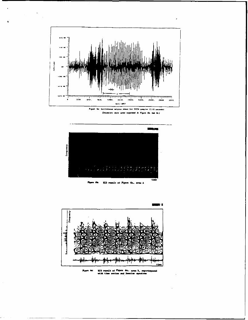
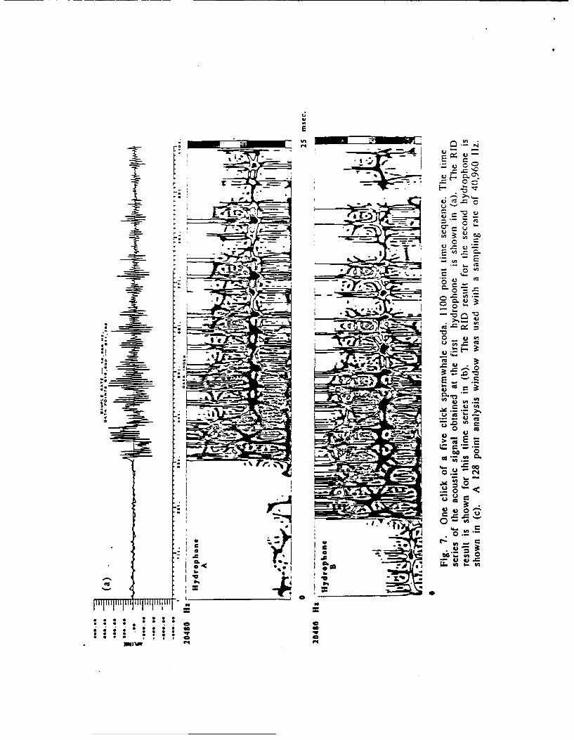
Figure 5. compares spectrogram and RID results for a TMJ click during jawmovement. Figure 6. shows RID results for a bottlenose dolphin. Note the relativeinvariance of the t-f patterns compared to the time series underneath. Thespectrum gives little hint of the t-f structure. Figure 7 shows RID results forspermwhale clicks. Note the repeated triplets in the data from the twohydrophones.

Conclusions

Williams-RID 4

1. RID produces very useful and interpretable results for natural signals. Uniquesignatures for underwater sounds seem to be an attractive feature andcapability of RID.

2. RID well represents what one would conceptually expect from an ideal time-frequency distribution in many situations.

3. The precise time and frequency structure of RID may allow source andmultipath structures to be disassociated.

4. Care must be taken in proper computation, display and interpretation ofresults.

5. There are conditions where the performance of RID is not as good as aspecialized distribution or approach designed to the signal and situation.

6. The RID possesses almost all of the desirable properties of a time-frequency distribution and is particularly useful in multicomponent situationswhere the reduced interference property is very desirable.

7. The Wigner distribution still has an important place in theory and inapplication, particularly when interference is not an issue, when one desires touse time-varying filtering and synthesis techniques and when signal detection isan issut. It may also be desired if cross terms are useful.

Acknowledgement

We are grateful for the collaboration of the group at Dr. Bill Watkin'sLaboratory at WHOI and the marine mammal sounds provided from theirdatabase - Dr. Watkins, Dr. Kurt Fristrup and Dr. Peter Tyack.

.. . .. . .. . ... .

I

Williams-RID 5

References

I L. Cohen, "Time-Frequency Distributions". IEEE Proceedings, July, 1989.

2 H. I. Choi and W. J. Williams. "Improved Time-Frequency Representation ofMulti-component Signals using Exponential Kernels. IEEE Trans. on ASSP, June,1989

3 W. J. Williams and J. Jeong., "Reduced Interference Time-frequencyDistributions," ISSPA Conf. and 1st Intl. Workshop on Time-FrequencyAnalysis and Its Applications, Gold Coast QLD, Australia, August, 1990.

4 P. Flandrin, "Some Features of Time-Frequency Representations of Multi-component Signals," IEEE Intl. Conf on ASSP, vol 3, pp. 41B.4.1-41B.4.4, 1984

5 F. Hlawatsch,"Interference Terms in the Wigner Distribution," in: DigitalSignal Processing -84. V. Cappellini and A. Constantinides (eds), pp. 363-367,North-Holland, 1984

6 W. A. Watkins. "The Harmonic Interval: Fact or Artefact in SpectralAnalysis of Pulse Trains," Marine Bio-acoustics, vol. 2., pp. 15-43, 1966.

Williams-RID 6

P5. nonnegazvty : pzt, 1; ) 0 :,/QO. 9 (u, r) is the ambiguity function of some function w(t).

Pi. realness : pz(t,f:g) E R

Qi. 9 (V, -r) = 9g(-v,-r)

P -. time shift : S(t) =--(t - t 0 ) => ps(, f; g) - t 0 ,f: g)Q2. g(v,-) does not depend on t.

P3. frequency shift : s(t) = z(t)ej 2 ,f0t =: Ps(t, f; g) = Pz(t, f - f: g)

Q3. g(v, -r) does not depend on f.

P4. time marginal " f 1V(tf)df = z(t)z'(t)

Q4. 9 (u, ) = IVV

PS. frequency marginal : fpz(tf;g)d = Z(f)Z-(f)0S.._q(0, r-) = I VT,

P6. instantaneous frequency f fp(tfg)d =fi(t)8g~u, ) f Pz(t'f;9 )df

Q6. Q4 and I- O = O0 W

P7. group delay: f t -(,f )

f9v? fpz(t~f~g)dtQ7. Q5 and lv-0 =0Vr

P8. time support : z(t) = 0 for It > tc = pZ(t,f;g) = 0 for Itj > tc

Q8. ¢(t, -) f"g',r,)ij 2 7td, = 0 for I < 21tj

Pg. frequency support : Z(f) = 0 for IflI > fc = pz(t, f: ) = 0 for 1fI > fc

Q9. fg(-,r ej27frdr = 0 for JvI < 2JfJ

PlO. Reduced Interference

QiO. g(v, r) is a 2-0 low pass filter type.

Table 1: Distribution properties and associated kernel requirements.

Distribution g(V, ) P0 Pi P2 P3 P4 PS P6 P7 P8 Pg PlO

Wigner 1 x x x x x x x x x

Rihaczek e) r x x x x x x

Re{Rihaczek} cos(fwr) x x x x x X X X X

Exponential (ED) e- ,2r 2 /u, x x x x x x x x

Spectrogram Aw(v,-r) of a window wa(t) x x x x x x

Born-Jordan* sin(rv-r) X X X x X X X X X X

Windowed-ED* e - 2 / , * W(V)lv=vr X X x x x x X X X X

' belongs to the RID.

Table 2: Comparison among several distributions.

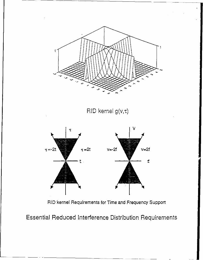
RID kernel g(v,tr)

f-2t Ir =2t v=-2f v-2f

RID kernel Requirements for Time and Frequency Support

Essential Reduced Interference Distribution Requirements

(a) ((C)

S Figure Ila.- lc. Kernels ofdifferentdisbutionsLi WD. b. spectrogram, c.R!LD

Figure ld. Amiguity function for signal in Figurc It

(d)Figure le.-lg. t-f distributions for two sinusoids:(d) CwD, f. specrogram, PLID

Figure 2. t-f distribuions for a chizp plus FM sign s:a. WD, b. specttoggu. -_ID

(a)

tnwhmWirhrau~i~mn in a) a): a)Z) D:7

ftaumaa a L.. . .. Z- 4 ! 0-a-O&

a Is C.1

~~~ x . :::x::::.x:x: lo a Oo'j . i ? A~~.

r CiCCC

(b)

(C)

FIGURE 3. A simulated sinusoid is pulsed 2 cycles on, 2 cycles off. 2 cycleson. 4 cycles oft;, 2 cycles on. 8 cycles off; 2 cycles on, 16 cycles off for the(a) spectrograrn, (b) Wigner distribution, and (c) RID. The analysis windowlength is 256 points in a&l cases.

-~--- -'-

zZC

- II

Jz

.0 I-o '0

zo 0

F;

C.

z-~-- -. ~- 0

zziizI Liz.AWA

*- ~

C

_____________ F I

- r -

z.aA.

zaI' A.

.4 aC,

1 A.

z .~ -II~ C, .4

Iz0

C,z

I~i 00 I,

II

I I

I II

Is. .2K..C,'

LTJ.4,,.

C,

f.4 pi

Pm.i °6

ACE,

oI

II

B 12.8 ms

ii .8s I I

time -

Spectrogram RID

c b. (

5 kd!z

FIGURE 5. TEMPOROMANDIBULAR (JAW) JOINT CLICK

1I 1- [I--nr P 1,rTm

"I. I.c

-In *4mlto ioa4&.a

OW I. il I Lm .* 1 ! 1 , 46 *!r I IF1~ 1514 T14. 1614 15111

p~~~jorm ~ ll *1U ea o im 6_Ar . rv

Withn6s Stck... lool Md 1mg off1 .alli*.(.1 ..

NNI2

- _ _ _ _ _.__ _ _ _ _-.d

Li.*r

eI u

W3 c

. -' " . .U -

I --

X..~

- t= s o4

h4

C6~ 160 ~

U2 6 PA

: : : : ",%

7P : -.

Iwa v

4b __ _ _ 4D

L ____________________________________________________P4___