reflectometry measurements on alcator c-mod
TRANSCRIPT

DOE/ET-51013-323
Reflectometry Measurements on Alcator C-Mod
Paul C. Stek
March 1997
This work was supported by the U. S. Department of Energy Contract No. DE-AC02-78ET51013. Reproduction, translation, publication, use and disposal, in whole or in partby or for the United States government is permitted.
PSFC/RR-97-5

Reflectometry Measurements on Alcator C-Mod
by
Paul Cornelis Stek
Submitted to the Department of Physics
in partial fulfillment of the requirements for the degree of
Doctor of Philosophy
at the
MASSACHUSETTS INSTITUTE OF TECHNOLOGY
March 1997
@ 1997 Massachusetts Institute of Technology. All rights reserved.
A uthor ......... .............. ...........................Department of Physics
March 11, 1997
Certified by........................... .................Dr. Jim Irby
Research Scientist, Experimental and Group LeaderThesis Supervisor
C ertified by .........................................................Professor Miklos Porkolab
Director of the Plasma Science & Fusion CenterThesis Supervisor
A ccepted by ........................................................Professor George Koster
Chairman, Physics Department Committee on Graduate Students
Reflectometry Measurements on Alcator C-Mod
by
Paul Comelis Stek
Submitted to the Department of Physicson March 11, 1997, in partial fulfillment of the
requirements for the degree ofDoctor of Philosophy
Abstract
This thesis presents the development of a novel millimeter wave reflectometer for thestudy of electron density profile evolution in the Alcator C-Mod tokamak.
The rate at which energy is transported from the center to the edge of a tokamakplasma is one of the main issues dictating the size and cost of future fusion reactors.A factor of two improvement in energy confinement time over basic operation or L-mode can be attained by operating in high or H-mode. The H-mode is characterizedby a transport barrier at the plasma edge.
To study the density profile and its evolution during H-mode a novel 5 channelmillimeter wave reflectometer was developed. With this diagnostic, electron densitygradients of 2 x 10 20m 4 have been observed during ELM-free plasmas within 0.5 msof the transition from L to H-mode. The width of the transport barrier was measuredto be less than 2 cm during the initial H-mode period.
Thesis Supervisor: Dr. Jim IrbyTitle: Research Scientist, Experimental and Group Leader
Thesis Supervisor: Professor Miklos PorkolabTitle: Director of the Plasma Science & Fusion Center
Acknowledgments
I am certain to omit many people here, and I apologize to those that I do omit.I want to start by thanking my advisor, Dr. Jim Irby, for his support over the
years and for his willingness to give me the freedom to make my own mistakes along
the way. I would also like to thank Professors Miklos Porkolab and Ian Hutchinson
for their teaching and efforts as readers of this thesis. The quality of this documenthas benefitted greatly from their efforts.
Thanks to all of the Alcatorians. There is hardly a student or member of the
engineering, technical, scientific, or support staff that has not taught me something
along the way. I will miss the free flow of ideas that characterize this group. A special
thanks to all of those who had to endure a conversation beginning with "Can I ask
you a dumb question...".To all my friends on the MIT Cycling Team: John"Voice of Reason" and Kjirste
"PowerBat" Morrell, Tom "the Sniveler" Moyer, "Smelly" Rich Pawlowicz,Jim "Tango" Preisig, "Joe Bob" Armstrong, Karon "Ronbo" MacLean, " nickname-
less" Jill Shirwood, and everyone else, I'll never forget the fun we had racing together
nor the joy of beating UMess at Easterns. Go MITTT!Thanks to my mother, father and, sisters who encouraged me through this expe-
rience.And thanks to Molly to have put up with me all these years. I don't know how I
will ever repay you, but I'll try.
3
Contacts
The author welcomes any questions regarding this research. I can be contacted at:
Jet Propulsion LaboratoryMicrowave Lidar, and Interferometer Technology SectionObservational Systems Division4800 Oak Grove DriveM/S 168-214Pasadena, CA 91109-80991-818-354-7749My E-mail address is currently unknown but will be available via the finger utilityusing "[email protected]".
The C-Mod reflectometer is left in the very capable hands of Yijun Lin ([email protected])under the guidance of Jim Irby ([email protected]).Earl Marmar ([email protected]) is head of Alcator diagnostics.Ian Hutchinson ([email protected]) is head of the Alcator research group.The general number for the PFC is (617) 253-8100.
Typesetting and Figures
This thesis was written using Latex version 2e by blindly following the path laid outby Dr. Darren Garnier Ph.D. M.o.L.a. Data figures were generated using IDL Version4 or MDS+. Hardware figures were generated with Claris-Cad and Auto-Cad.
'Master of Latex
4
Contents
1 Thesis Outline and Goals 15
1.1 Plasma Transport ....................... ....... 15
1.2 Alcator C-Mod . . . . . . . . . . . . . . . . . . . . . . . . . . . . . . 16
1.3 Plasma Diagnosis . . . . . . . . . . . . . . . . . . . . . . . . . .... 16
1.3.1 Reflectometry . . . . . . . . . .. . . . . . . . . . . . . . . . . 16
1.4 Thesis Goals . . . . . . . . . . . . . . . . . . . . . . . . . . . . . . 17
1.5 Thesis Outline . . . . . . . . . . . . . . . . . . . . . . . . . . . . . . . 17
2 Plasmas and Plasma Fusion 21
2.1 Plasm a . . . ... . . . . . . . . . . . . . . . . . . . . . . . . . . . . . . 21
2.2 Fusion . . . . . . . . . . . . . . . . . . . . . . . . . . . . . . . . . . . 22
2.3 Lawson Criteria . . . . . . . . . . . . . . . . . . . . . . . . . . . . . . 23
2.4 Magnetic Confinement . . . . . . . . . . . . . . . . . . . . . . . . . . 24
2.5 Tokamaks . . . . . . . . . . . . . . . . . . . . . . . . . . . . . . . . . 27
2.5.1 Flux Surfaces . . . . . . . . . . . . . . . . . . . . . . . . . . . 27
2.5.2 Impurities . . . . . . . . . . . . . . . . . . . . . . . . . . . . . 28
2.5.3 Limiters and Divertors . . . . . . . . . . . . . . . . . . .. .. 30
2.6 Energy Transport and H-Modes . . . . . . . . . . . . . . . . . . . . . 32
2.6.1 H-Mode Characteristics . . . . . . . . . . . . . . . . . . . . . 33
2.6.2 Model for Transport Barrier . . . . . . . . . . . . . . . . . . . 35
2.6.3 Issues for H-Modes in a Reactor . . . . . . . . . . . . . . . . . 36
5
3 Alcator C-Mod
3.1 Major Components . . . . . . . . . . . . . . . . . . . . . . . . . . ..
3.2 Diagnosing C-Mod Plasmas . . . . . . . . . . . . . . .. . . . . . . .
3.2.1 Two Color Interferometer . . . . . . . . . . . . . . . . . . . .
3.2.2 Core Nd:YAG Thomson Scattering . . . . . . . . . . . . . . .
3.2.3 Probes . . . . . . . . . . . . . . . . . . . . . . . . . . . . . . .
3.2.4 Magnetics and EFIT . . . . . . . . . . . . . . . . . . . . . . .
3.2.5 Electron Cyclotron Emission . . . . . . . . . . . . . . . .. . .
3.2.6 Spectroscopic Measurements . . . . . . . . . . . . . . . . . . .
3.3 Major Areas of Physics Research . . . . . . . . . . . . . . . . . . . .
3.3.1 Transport Scaling . . . . . . . . . . . . . . . . . . . . . . . . .
3.3.2 ICRF Heating . . . . . . . . . . . . . . . . . . . . . . . . . . .
3.3.3 Divertor Operation . . . . . . . . . . . . . . . . . . . . . . . .
3.3.4 Improved Confinement Modes . . . . . . . . . . . . . . . . . .
37
39
42
42
44
45
47
48
49
50
50
50
52
53
4 Reflectometry Theory 55
4.1 Dispersion Relations . . . . . . . . . . . . . . . . . . . . . . . . . . . 55
4.2 Accessibility in Toroidal Geometry . . . . . . . . . . . . . . . . . . . 58
4.3 Wave Propagation in a Stratified Medium . . . . . . . . . . . . . . . 63
4.3.1 Exact Solution for Linear Density Profile . . . . . . . . . . . . 64
4.3.2 The W.K.B. Method . . . . . . . . . . . . . . . . . . . . . . . 66
4.3.3 Profile Inversion . . . . . . . . . . . . . . . . . . . . . . . . . . 68
4.3.4 Hollow Profiles . . . . . . . . . . . . . . . . . . . . . . . . . . 69
4.4 Plasma Absorption and Emission . . . . . . . . . . . . . . . . . . . . 71
4.5 Relativistic Effects . . . . . . . . . . . . . . . . . . . . . . . . . . . . 72
5 The
5.1
5.2
5.3
5.4
Alcator C-Mod Reflectometer 75
Design Philosophy . . . . . . . . . . . . . . . . . . . . . . . . . . . . 75
Differential Phase or AM Reflectometry . . . . . . . . . . . . . . . . . 76
Choice of Frequencies and Polarization . . . . . . . . . . . . . . . . . 79
Transmitters and Receivers . . . . . . . . . . . . . . . . . . . . . . . . 80
6
5.5 Phase Detectors . . . . . . . . . . . . . . . . . .. .. . . . . . . . 85
5.6 Waveguides, Windows and Horns .................... 86
5.6.1 Waveguides ...................................... 86
5.6.2 Windows . . . . . . ... . . . . . . . . . . . . . . . . . . . . . 88
5.6.3 Horns . . . . . . . . . . . . . . . . . .. . . . . . . . .. . . . 88
5.7 Data Aquisition and Data Analysis . . . . . . . . . . . . . . . . . . . 91
6 Profile Reconstruction 93
6.1 Inversion Algorithm . . . . . . . . . . . . . . . . . . . . . . . . . . . . 93
6.2 Data Reduction . . . . . . . . . . . . . . . . . . . . . . . . . . . . . . 94
6.3 Calibration . . . . . . . . . . . . . . . . . . . . . . . . . . . . . . . . 99
6.3.1 High SOL Density Plasmas . . . . . . . . . . . . . . . . . . . 99
6.3.2 Comparison with Fast Scanning Probe . . . . . . . . . . . . . 102
6.3.3 Models for Probe Observations . . . . . . . . . . . . . . . . . 105
6.4 Comparison with Other Diagnostics . . . . . . . . . . . . . . . . . . . 110
6.4.1 Typical Features Observed with the Reflectometer . . . . . . . 110
6.4.2 Sawtooth Observations . . . . . . . . . . . . . . . . . . . . . . 111
6.4.3 Comparison with TCI and TS . . . . . . . . . . . . . . . . . . 114
6.4.4 Thomson Scattering Calibration . . . . . . . . . . . . . . . . . 114
7 Reflectometer Studies of H-modes 119
7.1 H-mode Characteristics . . . . . . . . . . . . . . . . . . . . . . . . . . 119
7.1.1 Edge Temperature Threshold . . . . . . . . . . . . . . . . . . 121
7.2 Electron Density Profile Evolution . . . . . . . . . . . . . . . . . . . . 124
7.2.1 ICRF Loading . . . . . . . . . . . . . . . . . . . . . . . . . . . 124
7.2.2 Profile Transition Time Scale . . . . . . . . . . . . . . . . . . 125
7.3 Fluctuation Suppression During H-mode . . . . . . . . . . . . . . . . 130
7.3.1 Note on Fluctuation Measurements . . . . . . . . . . . . . . . 131
7.3.2 Rate of Fluctuation Suppression at L-H Transition . . . . . . 132
7.3.3 Transport Barrier Width . . . . . . . . . . . . . . . . . . . . . 134
7.4 Enhanced D, H-modes . . . . . . . . . . . . . . . . . . . . . . . . . . 137
7

7.4.1 Post-Boronization . . . . . . . . . . . . . . . . . . . . . . . . .
8 Conclusions and Future Work 145
8.1 Conclusions ... ............................. 145
8.2 Future Reflectometry Work ...... ....................... 147
8.2.1 Reliability Improvement and Maintenance Reduction . . . . . 147
8.2.2 Calibration and Profile Reconstruction . . . . . . . . . . . . . 148
8.2.3 Cross Calibration Profile . . . . . . . .. . . . . . . . . . . . . . 148
8.2.4 X-Mode Polarization . . . . . . . . . . . . . . . . . . . . . . . 150
8.2.5 More Sophisticated Modulation Techniques . . . . . . . . . . . 151
8.2.6 Fluctuation Diagnostics . . . . . . . . . . . . . . . . . . . . . 151
8.3 More Ambitious Upgrades . . . . . . . . . . . . . . . . . . . . . . . . 153
8.3.1 ICRF Loading Studies . . . . . . . . . . . . . . . . . . . . . . 153
8.3.2 Eliminating Limiter Effects . . . . . . . . . . . . . . . . . . . 155
8.3.3 Higher Frequencies . . . . . . . . . . . . . . . . . . . . . . . . 155
8.4 Future H-Mode Work . . . . . . . . . . . . . . . . . . . . . . . . . . . 156
A DP Measurement of a Linear Profile 157
B List of Acronyms 165
8
137

List of Figures
1-1 Reflectometry Concept . . . . . . . . . . . . . . . . . . . . . . . . . . 18
1-2 Example H-mode Profile . . . . . . . . . . . . . . . . . . . . . . . . . 19
2-1 Progress Toward Plasma Fusion . . . . . . . . . . . . . . . . . . . . . 24
2-2 Schematic of a Tokamak . . . . . . . . . . . . . . . . . . . . . . . . . 26
2-3 Flux Surfaces . . . . . . . . . . . . . . . . . . . . . . . . . . . . .... 29
2-4 Limited and Diverted Plasmas . . . . . . . . . . . . . . . . . . . . . . 30
3-1 Alcator C-Mod Cross Section . . . . . . . . . . . . . . . . . . . . . . 38
3-2 Top View of Machine . . . . . . . . . . . . . . . . . . . . . . . . . . . 39
3-3 Alcator C-Mod Density Diagnostics . . . . . . . . . . . . . . . . . . . 43
3-4 Modeled TCI Measurements . . . . . . . . . . . .. . . . . . . . . . . 45
3-5 C-Mod Divertor Including Fast Scanning and Langmuir Probes. . . . 46
3-6 Example EFIT Reconstruction . . . . . . . . . . . . . . . . . . . . . . 47
3-7 B-Dot Coils . . . . . . . . . . . . . . . . . . . . . . . . . . . . . . . . 48
3-8 Visible Diode Array Views . . . . . . . . . . . . . . . . . . . . . . . . 49
3-9 The Two ICRF Two Strap Antennas . . . . . . . . . . . . . . . . . . 52
4-1 Coordinate System for Wave Propagation Derivation . . . . . . . . . 56
4-2 0 and X Mode Reflection . . . . . . . . . . . . . . . . . . . . . . . . 58
4-3 Cutoff Frequencies for 5.3 Tesla Plasma . . . . . . . . . . . . . . . . . 59
4-4 0-Mode Accessibility Plot for 5.3 Tesla . . . . . . . . . . . . . . .. . . 60
4-5 Accessibility Plot for 5.3 Tesla . . . . . . . . . . . . . . . . . . . . . . 61
4-6 Right Hand Cutoff and Upper Hybrid Resonance for 100 GHz . . . . 62
9
4-7
4-8
4-9
Accessibility Plot for 7.9 Tesla . .
Profile Kink . . . . . . . . . . . .
Hollow Profile Inversion Problems
4-10 Integration Paths
5-1
5-2
5-3
5-4
5-5
5-6
5-7
5-8
5-9
AM Technique . . . . . . .
Receiver Details . . . . . .
RF Source Box . . . . . .
Effect of Crystal IF Filter
I/Q Schematic . . . . . . .
Equipment Rack.....
A-Port Side View . . . . .
Horn Antennas . . . . . .
Horns in Machine . . . . .
6-1 Model Profile Inversion . . . . . . . . . . . . . . . . . . . .
6-2 Raw 110 GHz Data . . . . . .. . . . . . . . . . . . . . . . .
6-3 Example Raw Data . . . . . . . . . . . . . . . . . . . . . .
6-4 Example of Problem Raw Data . . . . . . . . . . . . . . .
6-5 Raw Data from High SOL Density Shot . . . . . . . . . . .
6-6 Fast Scanning Probe Mapping . . . . . . . . . . . . . . . .
6-7 Closeup of Mapping of Fast Scanning Probe for Two Shots
6-8 SOL Perturbation By Fast Scanning Probe . . . . . . . . .
6-9 SOL Perturbation by FSP at Higher Density . . . . . . . .
6-10 SOL Model . . . . . . . . . . . . . . . . . . . . . . . . . .
6-11 Density Measurements From FSP . . . . . . . . . . . . . .
6-12 Reflectometer View of a Turbulent Edge . . . . . . . . . .
6-13 Density Profile Evolution for Shot 950609011 . . . . . . . .
6-14 Crude Sawtooth Model . . . . . . . . . . . . . . . . . . . .
6-15 Sawtooth Mixing Radius . . . . . . . . . . . . . . . . . . .
6-16 Comparison of TCI, TS, and Reflectometer . . . . . . . . .
10
.
.
.
95
96
98
100
101
102
103
105
106
108
109
111
112
113
115
116
. . . . . . . . . .
63
68
70
71
77
81
82
84
85
86
87
89
90

6-17 TS Calibration from Reflectometer Cutoff . . . . . . . . . . . . . . .1
7-1 Radiation Limited H-mode . . . . . . . . . . . . . . . . . . . . . . . . 120
7-2 Edge Temperature Threshold . . . . . . . . . . . . . . . . . . . . . . 122
7-3 H-mode Profile and RF Coupling . . . . . . . . . . . . . . . . . . . . 123
7-4 Rate of L-H Profile Change . . . . . . . . . . . . . . . . . . . . . . . 127
7-5 Modeling TCI Through L-H Transition . . . . . . . . . . . . . . . . . 128
7-6 Modeling TCI Through L-H Transition (part 2) . . . . . . . . . . . . 130
7-7 Model of Scattering from a Rotating Mode . . . . . . . . . . . . . . . 131
7-8 Fluctuation Suppression Viewed by Reflectometer Channel Initially in
F SR . . . . . . . . . . . . . . . . . . . . . . . . . . . . . . . . . . . . 133
7-9 Outer Limit of Fluctuation Suppression Region During H-mode . . . 135
7-10 Inner Limit of Radial Extent of Fluctuation Suppression Region . . . 136
7-11 ELM-free and EDA H-mode . . . . . . . . . . . . . . . . . . . . . . . 138
7-12 Elm-free and EDA H-mode (part 2) . . . . . . . . . . . . . . . . . . . 141
7-13 FFT of Fluctuations during EDA H-mode . . . . . . . . . . . . . . . 142
7-14 EDA H-mode Fluctuation Frequency Modulated by Sawteeth . . . . . 143
8-1 Proposed Calibration Paddle . . . . . . . . . . . . . . . . . . . . . . . 149
8-2 Multiple Upconversion Frequency Concept . . . . . . . . . . . . . . . 152
8-3 Suggested Modifications for Single Sideband Study . . . . . . . . . . 154
A-1 Linear Profile . . . . . . . . . . . . . . . . . . . . . . . . . . . . . . . 158
A-2 Indistinguishable Profiles . . . . . . . . . . . . . . . . . . . . . . . . . 160
A-3 Linearized Profile . . . . . . . . . . . . . . . . . . . . . . . . . . . . . 161
11
117

12.
List of Tables
3.1 Alcator C-Mod Parameters . . . . . . . . . . . . . . . . . . . . . . . . 37
8.1 Electron Density Diagnostic Comparison . . . . . . . . . . . . . . . . 146
B.1 List of Acronyms . . . . . . . . . . . . . . . . . . . . . . . . . . . . . 165
13
ILi

Chapter 1
Thesis Outline and Goals
1.1 Plasma Transport
One of the key issues in the development of plasma fusion as an energy source is
learning how to predict and control the transport of particles and energy within the
plasma. Energy transport in a plasma is much faster than the diffusion predicted by
random collisions between plasma constituents. Collective effects driven, presumably,
by density and temperature gradients speed the transport of energy from the center
to the edge of the plasma. This has had a disastrous effect on the development of
commercial reactors as the faster energy is transported, the larger and more expensive
a reactor must become.
Kaye and Goldston [1] identified a baseline level of confinement named the Low
Mode or L-mode that virtually all tokamaks conform to provided no special efforts are
made. Several enhanced confinement modes of operation have also been observed (see
review by Stambaugh et. al. [21). In all such modes the turbulence that presumably
drives transport is suppressed in some portion of the plasma. The most common of
these enhanced confinement modes is the High Mode or H-mode first observed on the
ASDEX tokamak [3]. In this mode of operation, very large gradients in temperature
and density are observed at the outer edge of the plasma, indicating some form of
a transport barrier has formed there. Energy confinement in H-mode is two to four
times that during L-mode. Most reactor proposals plan on taking advantage of this
15
confinement enhancement.
1.2 Alcator C-Mod
Alcator C-Mod is a shaped and diverted follow-on to the very successful Alcator A
and C tokamaks. It is a compact tokamak capable of operating at nine tesla, 1.5
mega-amps of plasma current. With a main plasma volume of one cubic meter and
a combined ohmic and ICRF heating power of five megawatts, C-Mod has a power
density and divertor heat flux comparable to that expected on future reactors. As one
of only two large tokamaks commissioned in the last decade, C-Mod is a testing ground
for many new concepts in plasma science, particularly divertor operation and high
power density ICRF heating. With its high field and high current and power density,
C-Mod is well positioned to study plasma confinement in regimes complimentary to
those studied elsewhere.
1.3 Plasma Diagnosis
In order to study transport phenomena, accurate measurements of the local tem-
perature and density of electrons and ions and their gradients are needed. Despite
extensive effort devoted to plasma diagnosis, the electron temperature, via electron
cyclotron emission, is the only quantity that is routinely measured with high precision
and localization.
1.3.1 Reflectometry
Reflectometry is a diagnostic particularly well suited for studying the electron density
profile and fluctuations during H-modes. Based on the same concept as ionospheric
sounding, reflectometry involves launching microwaves into the plasma and measuring
the propagation time to some reflecting layer. For the polarization and frequencies
16

used in the C-Mod reflectometer, the index of refraction is given by:
2=c 2 k2 (We)2 n e2N 2 2 1 - where, w2
- (1.1)w 2 1me
where wp, is the electron plasma frequency. Figure 1-1 shows the basic concept of
reflectometry. A given frequency, f, is launched from the right towards the plasma.
At the position R,(f) where n = n,(f) the wave is reflected. By using multiple
frequencies and measuring the time a pulse takes to propagate to the reflecting layer
and back, the density profile can be determined a. A new diagnostic technique called
differential phase or amplitude modulated reflectometry is employed in this thesis.
This technique involves upconverting a fixed frequency and launching both sidebands.
The phase difference between the two returned signals gives the group delay with
very high time response. Figure 1-2 shows an example of the data obtained from the
reflectometer before and after an L-mode to H-mode transition.
1.4 Thesis Goals
The first goal of this thesis is the development of a diagnostic to measure the electron
density profile in the plasma edge in C-Mod. A five channel microwave reflectometer
with an innovative modulation scheme was developed for this. The second goal is
to study the time evolution of H-mode profiles in C-Mod. And, the third goal is to
distinguish between the varieties of H-modes seen on C-Mod.
1.5 Thesis Outline
The approach to studying Alcator C-Mod plasmas using reflectometry is outlined
below.
* Chapter two will introduce some of the basic concepts in tokamak physics in-
cluding energy and particle confinement.
'Dispersion is a major factor here and will be discussed in Chapter 4.
17

n
nQf)
0 Rjt) a
Figure 1-1: Reflectometry Concept Multiple frequencies arelaunched from the right, and the group delay to the cutofflayer and back is monitored.
" Chapter three will cover the Alcator C-Mod tokanak, some of the diagnostic
tools available, and the main research goals of C-Mod.
" Chapter four introduces the basic theories behind reflectometry.
" Chapter five presents the reflectometer diagnostic developed for C-Mod includ-
ing an innovative modulation scheme.
" Profile inversion, calibration, and comparison with other diagnostics is presented
in chapter six.
" Chapter seven discusses the electron density profile evolution during H-modes
in C-Mod. Fluctuations and ELM's during the various types of H-modes seen
on C-Mod will also be presented.
" In Chapter eight, conclusions and recommendations for future work are pre-
sented.
18
Thomson Scattering L-Mode (0.80 s)ThrsnSecaiering H-M-de (1 , s)
Reflectometer L-Mode (0.80 s)Ref'ectm't-r H -M d (C.2 'I
Center LCFSI . ., 1
0.75 0.80Major Radius (m)
0.85 0.90
Figure 1-2: Example H-mode Profile Shot 950602028. During anH-mode, the profile steepens greatly near the last closedflux surface (LCFS). The high gradient can form in lessthan 1 ms. (The absolute calibration of the Thomsonscattering is suspect for reasons to be discussed.)
19
2.0
1.5
E0
C
C)0
1.0
0.5
onPIOsmO
0.7000
1
* In Appendix A the group delay measured for a linear profile is presented along
with a matrix technique for inverting a piecewise linear profile.
* Appendix B is a table of some of the many acronyms used in this thesis with
references to the first usage.
20
Chapter 2
Plasmas and Plasma Fusion
In this chapter, plasmas, plasma fusion, and tokamaks will be presented. The in-
tention is that a reader with little prior knowledge of fusiona will understand the
motivation for the research presented in later chapters. A more detailed introduction
to plasma physics can be found in Chen [4]. Wesson [5] is an excellent, though quite
expensive, reference on tokamaks.
2.1 Plasma
A plasma is gas in which at least a fraction of the atoms present are ionized. They
are typically characterized by high electrical conductivity. Some common plasmas are
welding arcs, lightning, and the discharges in fluorescent light bulbs. While in these
plasmas only a small fraction of the constituent gas is ionized, their conductivity is
dominated by this small ionized fraction. Plasma is often referred to as the fourth
state of matterb, and in fact only 0.5 percent of the known universe is in the first
three states: gas, liquid, and solid. Most of the rest is plasma.
Despite the cosmological disposition of matter to be ionized, plasmas are relatively
'Like the wife of the author who is proofreading this.'It should be noted that the other three states, under most conditions, will have a well defined
phase transition and phase boundary. There is no such boundary or transition between a gas anda plasma. The naming of an object as either a gas or a plasma in many cases reflects more on theanalysis being performed. In addition, designating plasmas the fourth state of matter opens thedoor to a host of other conditions that could lay claim to being a state of matter such a neutronstar or a black hole.
21
remote from the average human's existence.c And while fluorescent lights and arc
welders are useful appliances, their understanding hardly warrants the $ 1 billion
annual worldwide budget for plasma research. In fact, most of the study of plasmas,
the subject of this thesis included, is directed towards the development of nuclear
fusion as a "cleaner" energy source for the future.
2.2 Fusion
Nuclear fusion is the combining of two nuclei to form a larger nucleus and usually a
free neutron or proton. The source of the energy given off by most stars is the fusing
of hydrogen into heliumd (a fact only recognized early this century). While there is a
very long list of possible fusion reactions, the most promising ones for terrestial power
production aree:
D 2 + T3 -+He 4+ n'+17.6MeV (2.1)
D 2 + D 2 -+He 3 + n'+3.27MeV (2.2)
D 2 + D 2 - T 3+HI+4.03MeV (2.3)
D2 +He3 -+H e+H 1 +18.3MeV [5] (2.4)
There is a direct analogy between fusion reactions and the chemical reactions that
may be more familiar such as burning methane:
CH4 + 202 -+ CO2 + 2H 20 + Heat (2.5)
First, this reaction will proceed provided the activation energy is provided. However,
if one wants to ignite the reactants, one must transfer some of the resulting heat
to the other reactants to provide their activation energy. To maintain ignition, one
CEnterprise and Voyager crew members excepted.dFor stars fainter than the sun, this fusion is accomplished by direct proton-proton reactions. For
stars brighter than the sun, the conversion of of hydrogen to helium is catalyzed by carbon [6].e MeV = 106 electron volts = 1.6 x 10⁻¹³ joules. The electron volt is also used as a unit of
temperature in plasma physics where I eV = 1.1605 x 10' K.
22

needs to keep the reactants hot enough, long enough, and with sufficient density to
make the reaction self-sustaining.
The same principles apply to fusion. While a fusion reaction liberates a million
times more endrgy than a typical chemical reaction, the Coulomb repulsion of the
nuclei makes the activation energy higher by the same factor. For two nuclei to fuse
they need to get close enough for their wavefunctions to overlap significantly. The
cross-section for deuterium-tritium (DT) fusion, the most likely initial fusion fuel, has
a maximum at over 100 keV.
2.3 Lawson Criteria
Lawson [7} set a lower limit for the performance of a fusion reactor. A self-sustaining
reactor would need to heat some quantity of fuel and confine the hot fuel long enough
and at sufficient density to produce enough fusion energy to provide the electricity
needed for the heating of the original quantity of fuel. Lawson found that at 20 keV
the product of the density, n, and energy confinement time, TE, must be:
nfTE > 6 x 101m9-3S. (2.6)
This is now known as the Lawson Criterion or " break even". Achieving this criteria
has been a goal of the fusion community for the last 40 years, but only recently
have experiments come close to achieving the required temperature, density, and
confinement time simultaneously (Q = 1 in Fig. 2-1).
Most practical fusion schemes, however, require far better parameters than those
set out by Lawson's Criteria. "Ignition" (Q = oo in Fig. 2-1) requires that enough en-
ergy from the fusion products be confined within the plasma to maintain its temperaturef.
Producing a tokamak capable of producing igniting plasmas is arguably the next step
after the current set of tokamak experiments. The International Tokamak Experi-
mental Reactor or ITER is the current embodiment of this goal. Much of the work
-fNote that for DT fusion, 80% of the fusion energy is carried by the neutron which does notinteract with the plasma. This greatly adds to the fusion challenge.
23

10.00
__ 1.00
E0
0.10
C:
c
0.01
0.1
X TFTR(86)
Alcator c(83) x
Alcator A KTFTR(85) *
DII(84) W,AIcator A
PLT(79) X
Q=oo
JET(88 JET(89)K C-Mod(96) - -- JT (93)-X JT60(87) T DIR(D(91)
DIIID(87) X TFTR(87)
ASDEX(84)
TFR(75) )
ST(7 )K
W T3(68)
SPDX(51)
X PLT(78)
I -
10.0 100.0Ti(keV)
Figure 2-1: Progress Toward Plasma Fusion [8] Fusion boosterspoint out that over the last 25 years the percentage in-crease in the fusion triple product nrT compares favor-ably with the growth in the number of devices per unitarea on a microprocessor chip. Note that C-Mod hasperformance parameters comparable to machines such asJET that have 100 times C-Mod's plasma volume at 10times C-Mod's cost.
on smaller machines such as Alcator C-Mod is conducted with the design and devel-
opment of ITER, or some device like it, in mind.
2.4 Magnetic Confinement
Now that the desirability of creating extremely hot plasmas that stay hot for a signifi-
cant period of time has been established, how does one do this on earth in a controlled
manner? The obvious problem is heat transfer from the plasma to the vessel confin-
ing it. While many approaches to confining the hot plasma have been suggested, the
24
most developed technique is through magnetic confinement.
A plasma may be confined using a strong magnetic field. A particle with charge
q moving in a magnetic field B feels a force perpendicular to both the magnetic field
and its velocity: F = q(v x B). As a consequence, in a uniform magnetic field with no
electric field present, charged particles stream freely along the field lines but gyrate
about the field lines with a gyro (Larmor) radius and frequency given by:
rt = - _ =B (2.7)qB m
In the presence of an electric field, the kinematics become more complicated. The
particle is free to accelerate due to the component of E parallel to B; however, the
component of E perpendicular to B produces a drift9 perpendicular to both E and
B:
VExB = E x B/B 2 . (2.8)
If the field lines are curved, the drifth relative to the B field lines due to the centrifugal
force and the radial variation in the field (dictated by V - B = 0) is given by:
m RK B /,, ',,\
v, ± Va = mR!xB2 o + ). (2.9)
Any confinement scheme must at least provide E and B fields such that ionized
particles are confined subject to these drifts.
An engineering principle is that breaks in symmetry lead to stress concentrations
that limit the strength of a structure. Presumably the higher the magnetic field the
better the plasma will be confined, so a symmetric shape for magnetic confinement
is probably desirable. The current shortage of magnetic monopoles dictates that
V - B = 0, precluding the possibility of a spherically symmetric magnetic confinement
device. Cylindrical symmetry with B along the axis of symmetry (z) fails because
25
gLogically known as the "E x B" drift.hCalled the curvature drift.
Toroidal Magnetic Field Coil
Equilibrium Field Coils
Ohmic Transformer Stack
Vacuum Vessel
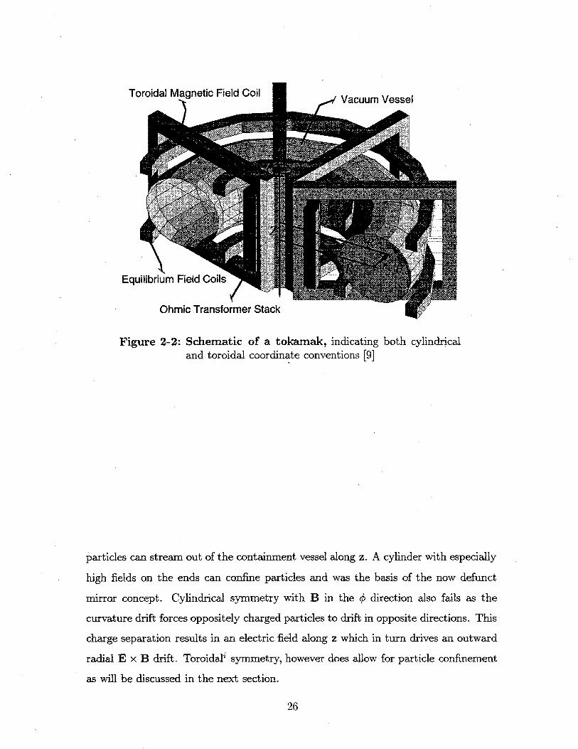
Figure 2-2: Schematic of a tokamak, indicating both cylindricaland toroidal coordinate conventions [9]
particles can stream out of the containment vessel along z. A cylinder with especially
high fields on the ends can confine particles and was the basis of the now defunct
mirror concept. Cylindrical symmetry with B in the 0 direction also fails as the
curvature drift forces oppositely charged particles to drift in opposite directions. This
charge separation results in an electric field along z which in turn drives an outward
radial E x B drift. Toroidal' symmetry, however does allow for particle confinement
as will be discussed in the next section.
26
2.5 Tokamaks
Currently the tokamak' is the most promising concept for producing the first fusion
reactor. A strong toroidal field is provided by the large toroidal field coils shown in
Fig. 2-2. To avoid the vertical charge separation and resultant radial E x B drift
discussed in the previous section, a poloidal field is introduced which allows particles
streaming along a field line to short out any vertical E field. This poloidal field can
only be provided by a toroidal current running in the plasma. The plasma current
is driven by induction. Current is ramped through a coil passing through the center
of the torus. This produces a change in magnetic flux through the torus, inducing a
toroidal voltage and current in the plasma. External field coils provide the vertical
field needed for radial force balance and allow for shaping of the plasmak
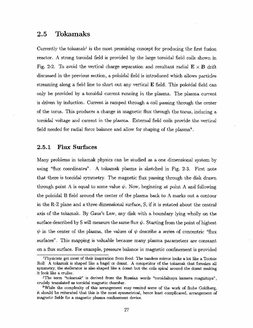
2.5.1 Flux Surfaces
Many problems in tokamak physics can be studied as a one dimensional system by
using "flux coordinates". A tokamak plasma is sketched in Fig. 2-3. First note
that there is toroidal symmetry. The magnetic flux passing through the disk drawn
through point A is equal to some value 4. Now, beginning at point A and following
the poloidal B field around the center of the plasma back to A marks out a contour
in the R-Z plane and a three dimensional surface, S, if it is rotated about the central
axis of the tokamak. By Gaus's Law, any disk with a boundary lying wholly on the
surface described by S will measure the same flux 4. Starting from the point of highest
4 in the center of the plasma, the values of 4 describe a series of concentric "flux
surfaces". This mapping is valuable because many plasma parameters are constant
on a flux surface. For example, pressure balance in magnetic confinement is provided
TPhysicists get most of their inspiration from food: The tandem mirror looks a lot like a TootsieRoll. A tokamak is shaped like a bagel or donut. A competitor of the tokamak that forsakes allsymmetry, the stellerator is also shaped like a donut but the coils spiral around the donut makingit look like a cruller.
'The term "tokamak" is derived from the Russian words "toroidalnaya kamera magnitnya?',crudely translated as toroidal magnetic chamber.
kWhile the complexity of this arrangement may remind some of the work of Rube Goldberg,it should be reiterated that this is the most symmetrical, hence least complicated, arrangement ofmagnetic fields for a magnetic plasma confinement device.
27

by J x B = Vp. In addition, since b is constant on a flux surface, B -Vo = 0. By
symmetry, both V0 and Vp lie in the R-Z plane. Since both are perpendicular to B,
V0 and Vp are everywhere parallel, hence p can be described as a function of 4.Another flux surface quantity is the safety factor, q. Again in Fig. 2-3, if one
begins at point A and follows a field line as it travels along the surface S until one is
again at the same poloidal location as A, the number of times one has traversed the
tokamak toroidally is q. When q is a rational number, a perturbation on a flux surface
can be resonant. Often, q = 1 near the center of the plasma. This can result in a
relaxation oscillation called a sawtooth that limits the current density at the center
of the plasma.1 The current profile in most tokamak plasmas is peaked on axis, so
q increases as one moves out from the center. Higher q increases plasma stability.
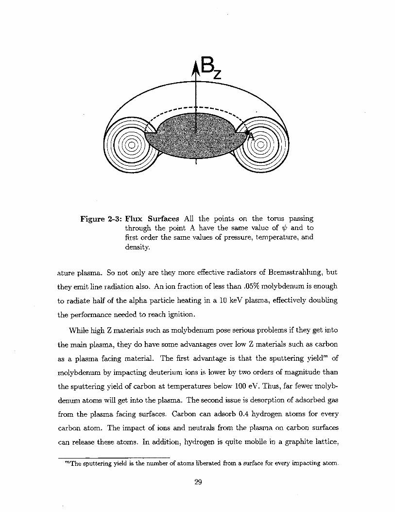
A higher toroidal current improves confinement, but lowers q. By elongating the
plasma, q at the edge can be kept high while raising the current. The left hand figure
in Fig. 2-4 shows an elongated plasma. The ratio b/a is the elongation, n.
2.5.2 Impurities
Preventing plasma contamination by impurities is a major hurdle along the road to
building a fusion reactor. The first problem posed by impurities is dilution of the
reactants. At reactor temperatures (- 20 keV), light elements such as carbon and
oxygen will be fully stripped of their electrons. For every percent of ions that are
oxygen, an eight percent increase in the electron density and the Lawson criteria is
required. In addition, alpha particles produced in a burning plasma will also dilute
reactants. Once the alphas have deposited their energy in the plasma, they need
to be swept out in some way. To make matters worse, in many regimes, impurities
accumulate in the center, diluting the plasma where it is most reactive.
The other and generally more critical issue is radiative energy loss due to impu-
rities. Because light elements such as carbon and oxygen are fully stripped in a hot
plasma, Bremsstrahlung is the dominant radiation mechanism. The heavier elements
such as iron, tungsten and molybdenum are not fully stripped in a reactor temper-
'In fact, almost all plasmas on Alcator C-Mod have sawtooth oscillations.
28
B
Figure 2-3: Flux Surfaces All the points on the torus passingthrough the point A have the same value of V, and tofirst order the same values of pressure, temperature, anddensity.
ature plasma. So not only are they more effective radiators of Bremsstrahlung, but
they emit line radiation also. An ion fraction of less than .05% molybdenum is enough
to radiate half of the alpha particle heating in a 10 keV plasma, effectively doubling
the performance needed to reach ignition.
While high Z materials such as molybdenum pose serious problems if they get into
the main plasma, they do have some advantages over low Z materials such as carbon
as a plasma facing material. The first advantage is that the sputtering yieldm of
molybdenum by impacting deuterium ions is lower by two orders of magnitude than
the sputtering yield of carbon at temperatures below 100 eV. Thus, far fewer molyb-
denum atoms will get into the plasma. The second issue is desorption of adsorbed gas
from the plasma facing surfaces. Carbon can adsorb 0.4 hydrogen atoms for every
carbon atom. The impact of ions and neutrals from the plasma on carbon surfaces
can release these atoms. In addition, hydrogen is quite mobile in a graphite lattice,
mThe sputtering yield is the number of atoms liberated from a surface for every impacting atom.
29
Edge
X point
FRzStrike Points
Figure 2-4: Limited and Diverted Plasmas The figure on the leftis a cross section of a limited plasma with an elongationof , = b/a. Impurities generated at the plasma/wall in-terface (limiter) are free to enter the main plasma. Onthe right is a diverted plasma. Note that the plasma/wallinterface (strike points) are well removed from the mainplasma.
so a hydrogen inventory tens or hundreds of times the plasma inventory is available
in the walls of a carbon tiled machine. As a result, neutral and plasma density can
be difficult to control in a carbon tiled machine.
2.5.3 Limiters and Divertors
The plasma must at some point contact a material surface. At this interface, ener-
getic ions can sputter atoms off the surface. These atoms can then enter the main
plasma. In addition, atoms adsorbed on the surface can be liberated by incident
ions. Typically there is a dynamic equilibrium between the rate of incidence and of
desorption, so a material surface can act like either a pump or a source. Also, as a
surface is heated, adsorbed atoms are liberated. And of course the material can melt,
30
Limiter
b
4:
LCFS Core

sublimate, or fracture if the constant or temporary heat load on the surface is too
high.
The simplest technique for providing a plasma/solid interface is a limiter, shown
on the left in Fig. 2-4. Here, the edge of the plasma is defined by a piece of material
designed to withstand the heat load from the plasma. The main problem with this
arrangement is that atoms liberated from the limiter surface by impacting ions are
free to enter the main plasma. This problem can be avoided in principle by using a
magnetic divertor, shown on the right in Fig. 2-4. Particles that exit the main plasma
stream along the magnetic field lines to contact material walls well removed from the
main plasma.
The "last closed flux surface" (LCFS) or "separatrix" is the outermost flux surface
that encircles the plasma without contacting a material surface. The "X-point" is
the point on the LCFS where the magnetic field is exactly toroidal. From this point,
particles on a flux surface can either circle the plasma or go to the divertor. The
points where the LCFS intersect the divertor plates are the inner and outer strike
points. The "'core" plasma is the central portion of the plasma. Its boundary is not
precisely defined, but can be taken as the region where the temperature is at least
30% of the central temperature. The "edge" plasma is the plasma outside of the core
plasma. The "scrape-off layer" (SOL) is the plasma outside of the LCFS, a subsection
of the edge. The "private flux region" (PFR) is the region below the separatrix in
the divertor region.
The divertor has four functions. First, it provides a boundary for the plasma
that is not a material surface. Second, neutrals and neutral impurities entering the
scrape-off layer are ionized and pumped to the divertor, away from the main plasma.
Third, along the path to the strike point, the plasma can be cooled through collisions
to reduce sputtering at the strike point. And fourth, the heat destined for the strike
points can be dissipated by intentionally introducing impurities to cool the plasma
through radiation. This is called a "dissipative divertor".
31
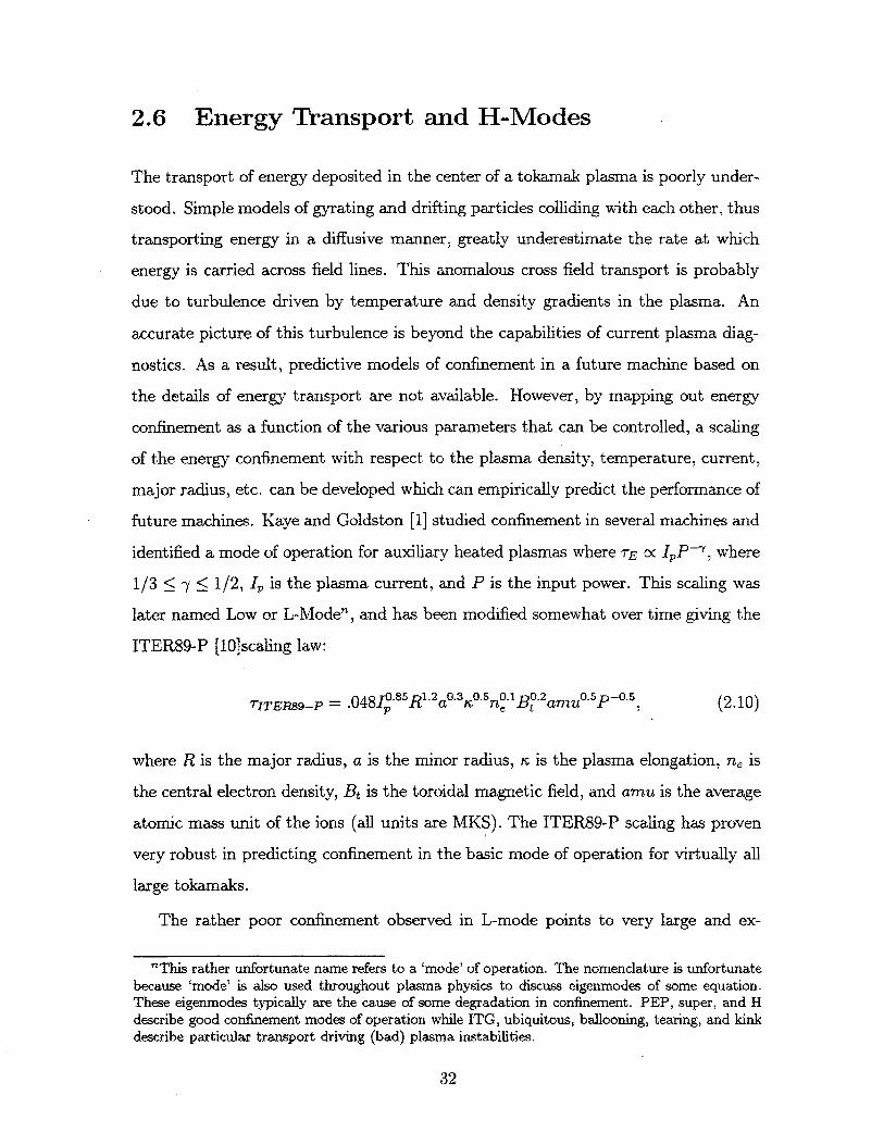
2.6 Energy Transport and H-Modes
The transport of energy deposited in the center of a tokamak plasma is poorly under-
stood. Simple models of gyrating and drifting particles colliding with each other, thus
transporting energy in a diffusive manner, greatly underestimate the rate at which
energy is carried across field lines. This anomalous cross field transport is probably
due to turbulence driven by temperature and density gradients in the plasma. An
accurate picture of this turbulence is beyond the capabilities of current plasma diag-
nostics. As a result, predictive models of confinement in a future machine based on
the details of energy transport are not available. However, by mapping out energy
confinement as a function of the various parameters that can be controlled, a scaling
of the energy confinement with respect to the plasma density, temperature, current,
major radius, etc. can be developed which can empirically predict the performance of
future machines. Kaye and Goldston [11 studied confinement in several machines and
identified a mode of operation for auxiliary heated plasmas where rE oc IpP-I, where
1/3 < -t 1/2, Ip is the plasma current, and P is the input power. This scaling was
later named Low or L-Mode", and has been modified somewhat over time giving the
ITER89-P [10]scaling law:
TITER89-P = .048I0 8 5R 2 a 0 .s3 0 5 .1B0 2 amuosP-0 5, (2.10)
where R is the major radius, a is the minor radius, rn is the plasma elongation, n, is
the central electron density, Bt is the toroidal magnetic field, and amu is the average
atomic mass unit of the ions (all units are MKS). The ITER89-P scaling has proven
very robust in predicting confinement in the basic mode of operation for virtually all
large tokamaks.
The rather poor confinement observed in L-mode points to very large and ex-
"This rather unfortunate name refers to a 'mode' of operation. The nomenclature is unfortunatebecause 'mode' is also used throughout plasma physics to discuss eigenmodes of some equation.These eigemnodes typically are the cause of some degradation in confinement. PEP, super, and Hdescribe good confinement modes of operation while ITG, ubiquitous, ballooning, tearing, and kinkdescribe particular transport driving (bad) plasma instabilities.
32
pensive fusion reactors. This unfortunate result has encouraged extensive research
into operating regimes with better than L-Mode confinement. Stambaugh et al. [2]
reviewed research in "Enhanced Confinement Modes" of operation. They distinguish
between two groups: those characterized by peaked density profiles, and those with
flat density profiles. The first group includes PEP (Pellet Enhanced Performance),
Super, and IOC (Improved Ohmic Confinement) modes. The improved confinement
of all of these modes is assumed by many to be due to suppression of the ion temper-
ature gradient (ITG) mode'. Plasmas having density profiles that are more peaked
than the ion temperature profile are believed to be stable to this mode. The second
group of enhanced confinement modes consists of the many variations of "High" or
"H-Mode" which will be discussed below.
2.6.1 H-Mode Characteristics
Groebner [11] provides a recent review of H-mode experimental observations. The
US-Japan Workshop on H-Mode Physics [12] is a comprehensive and up to date (1995)
presentation of the current status of H-mode experiments and theory worldwide. The
H-mode was first seen on ASDEX [3] in 1982 and has since been observed on virtually
all high performance tokamaks. Above some threshold edge temperature or applied
heating power, a transport barrier can form in the plasma edge resulting in greatly
improved global particle confinement and typically a factor of two improvement in
global energy confinement over L-mode levels. Typically, H-modes are observed dur-
ing divertor operation, though they have been observed on some limiter machinesP.
H-modes have also been induced in low input power tokamaks by biasing the plasma
relative to the vacuum chamber.
In diverted plasmas, several phenomena characterize the transition from L-mode
to H-mode (L-H transition). The two most apparent phenomena are a dramatic
'Originally known as the r7i mode.PRather than reference individual machines, the interested reader is referred to the papers by
Groebner and Stambaugh cited above.
33

rise in the plasma density and a drop in D-alpha emission". The rise in density
appears to be the result of improved particle confinement, while the drop in the D-
alpha emission is a signature of a decrease in the recycling of deuterium in the SOL.
It is important to note that while the drop in D-alpha emission does indicate an
increase in the confinement time of the whole plasma (SOL and PFR included!), it
does not directly translate to a change in the core plasma particle confinement. As
the H-mode progresses, the recycling light may return to or even exceed the original
emission levels.
Other key phenomena observed at the L-H transition are an increase in the electron
density inside the LCFS and a drop in the density outside the LCFS. In the steep
gradient region (SGR) near the LCFS, density fluctuations appear to be suppressed
in H-mode. The electron temperature typically increases at the transition. Other
characteristics observed with the proper diagnostic set include a dramatic increase in
impurity confinement and a large sheared poloidal rotation in the SGR. Typically, the
core density and temperature profiles during H-mode are flatter than during L-mode
operation. Edge Localized Modes (ELMs) appear in most long duration H-modes and
can be identified as bursts of D-alpha emission and magnetohydrodynamic (MHD)
fluctuations. ELMs come in many varieties and are a temporary relaxation of the high
pressure gradient at the edge. In some machines as much as 5% of the plasma's stored
energy can be released in a single 1 ms ELM, making ELMs the source of the highest
peak heat loads in these machines. While ELMs do degrade energy confinement, they
also appear to control the buildup of impurities and control the rise in plasma density.
An ELM-free H-mode with low recycling is always a transient phemonena as impurity
radiation and uncontrolled density rise eventually lead to a cooling of the SGR and
a return to L-mode.
Operationally, four other factors affect access to and maintenance of H-modes.
The first is wall cleanliness and conditioning. Presumably, low neutral pressure and
qThese phenomena can occur for reasons other than an L-H transition. For example, impurityinjections, MARFEs, and changes in divertor operation can greatly change the plasma density andD-alpha emission. Distinguishing periods of H-mode operation from these other phenomena duringearly C-Mod operation was something of a challenge.
34
low impurity levels aid in achieving the high edge temperatures required for H-mode
operation. Second, the size of the gap between the LCFS and any walls or limiters
needs to be as large as practical with the particular heating scheme being used. This
also is probably related to reducing sputtering or desorption of impurity and majority
atoms. Third, the direction of the ion B x VB drift should be towards the divertor.
Directing the ion B x VB drift away from the divertor typically requires twice the
input power to achieve H-mode. Fourth, the density must be within some range for
a given input power. A low density limit has been seen on most machines. While the
cause of the low density limit is not clear, higher impurity fractions, locked modes,
and smaller sawteeth are possible reasons. The upper density limit is related to the
energy density achievable for a given input power and the temperature needed to
achieve H-mode.
Energy confinement during H-mode is typically twice the value expected with
ITER89-P scaling and is generally believed to be largely due to a suppression in
transport at the edge. Both JET and DIII-D have achieved H factors approaching
four during "Hot Ion H-modes" on JET and during "VH-modes" on DIII-D. In the
VH-modes, poloidal rotation and suppressed fluctuations extend inward over most of
the plasma radius, apparently combining the good qualities of both central and edge
enhanced confinement regimes.
2.6.2 Model for Transport Barrier
All machines that attain H-modes and have the capability to measure significant
plasma rotation observe a sheared poloidal plasma rotation during H-mode. This
shear is most likely caused by an E x B drift, driven by a radial electric field, E T .
The interested reader is referred to the review article by Ward [131. A sheared flow
perpendicular to a density gradient decorrelates the convective eddies that drive the
transport. The skewed eddies are thus more heavily damped by the increased relative
speed between eddies. In addition, the skewed eddies break up into smaller eddies,
'The source of this electric field, is the cause of much speculation and is beyond the scope of thisthesis.
35

reducing the step size for a volume of plasma moving across the pressure gradient.
Together, these effects enable a sheared flow to produce a transport barrier.
2,.6.3 Issues for H-Modes in a Reactor
Current plans for test reactors such as ITER count on obtaining a factor of two im-
provement in energy confinement by running in H-mode rather than L-mode. How-
ever, operating in H-mode presents five major challenges, three of which, ironically,
are a result of overly good particle confinement. The first problem is the accumula-
tion of impurities and helium. Some mechanism needs to be developed to sweep out
impurities and ash without significantly reducing energy confinement. The second
issue is controlling the density in H-mode. As the plasma density rises, the heating
power needed to reach ignition temperatures also goes up. Third, the low SOL density
seen in H-modes reduces the coupling of ICRF and lower-hybrid waves to the plasma,
reducing the power launched per unit area of antenna. Fourth, the high peak heat
loads due to type one ELMs complicate divertor designs. And fifth, the high edge
temperatures required for H-mode operation are difficult to incorporate in dissipative
divertor concepts.
36
Chapter 3
Alcator C-Mod
The Alcator C-Mod" (hereinafter "C-Mod") tokamak is the third of the Alcator line
of tokamaks built at the Massachusetts Institute of Technology. Alcator A and Alca-
tor C6 were both compact, high magnetic field, high electron density tokamaks with
circular poloidal cross-sections. C-Mod was built to test shaped and diverted plas-
mas in a compact, high magnetic field tokamak. As the only large tokamak to be
commissioned in the United States in the last decade, C-Mod benefits from and tests
some of the latest concepts in plasma physics and fusion technology.
aC-Mod was originally proposed as a modification of the Alcator C tokamak, hence the name"C-Mod". However, as the design work progressed it became clear that very little of the originalmachine could be used. In fact, rather than being modified for use in C-Mod, the Alcator C vacuumchamber, power supplies, and magnets were shipped to Lawrence Livermore National Lab wherethey became the MTX experiment.
bCommissioned in 1973 and 1979, respectively.
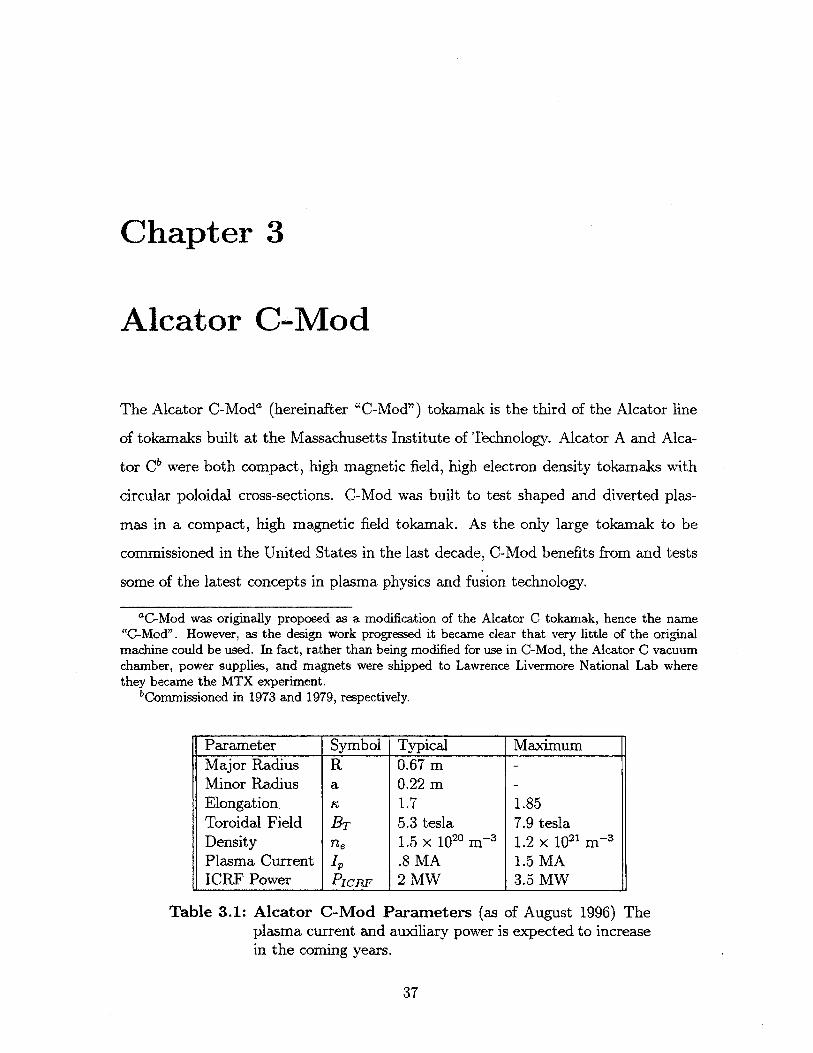
Parameter Symbol Typical MaximumMajor Radius R 0.67 mMinor Radius a 0.22 m -Elongation r 1.7 1.85Toroidal Field BT 5.3 tesla 7.9 teslaDensity n, 1.5 X 10²⁰ m-3 1.2 x 10²¹ m-3Plasma Current I, .8 MA 1.5 MAICRF Power PICRF 2 MW 3.5 MW
Table 3.1: Alcator C-Mod Parameters (as of August 1996) Theplasma current and auxiliary power is expected to increasein the coming years.
37
VERTICAL PORTS 1200LBS
DRAW BAR IG,560LBS
RINGS D20LBS
UPPER COVER 57,680LBSDOWEL P[NS 670LBS
LOCK PINS lI15GLBSUPPER WEDGE PLATE 10,750LBS
CYLINDER 44,000LBSEF-4 MOUNTING BRACKETS 2JOOLS
I0T) EF COILS 10,500LBS
PLASMA 0,000002LBS
tles 4,B30Tbs
TAPERED PINS 68OLBSLOCK SCREWS 240LBS
LOWER WEDGE PLATE 10,750LBSLOWER COVER 57,680LBS
CRYOSTAT 5,060LBS
pVERT[CAL PORT FLANGES 200LrOH COIL 3,00 OLDS TF MAGNET 48000,LBS
MOUNT
HO
HOR
ING PLATE-TOP I800LBS
RIZONTAL PORTS 50OLDS
IZONTAL PORT EXTENT[ONS 1,700LBS
HORIZONTAL PORT FLANGES 300LBS
VACUUM CHAMBER 6,000LES
MOUNTING PLATE-BDTTOM 1,800LBS
I-
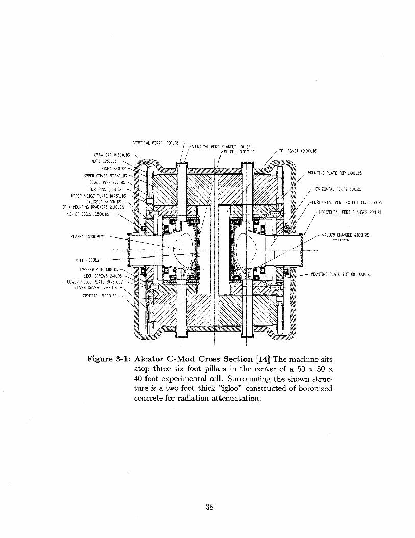
Figure 3-1: Alcator C-Mod Cross Section [14] The machine sitsatop three six foot pillars in the center of a 50 x 50 x40 foot experimental cell. Surrounding the shown struc-ture is a two foot thick "igloo" constructed of boronizedconcrete for radiation attenuatation.
38

D GFast Scanning Probe Port
RF Antennas Thomson Scattering Port
C TOl Port H
TF Coils
AB Limiter PlasmSupport Cylinder
Reflectometer Horns Proposed 4 strap Antenna /
Bu Cryostat
WR42 WaveguideK
A Bus Tunnel
Figure 3-2: Top View of Machine The diameter of the cryostat isapproximately four meters. The major density diagnos-tics are labeled.
3.1 Major Components
C-Mod developed from the collaboration of scientists and engineers from many disci-
plines. No physics thesis is complete without at least pointing out a few of the major
engineering efforts involved in building and running this machine.
Vacuum Chamber: The stainless steel C-Mod vacuum chamber is unique in
several ways. First, it is a torus without a poloidal insulating break. This allows
the chamber to be strong enough to support the poloidal field coils. This is key to
producing a shaped, compact, high field tokamak because there is no space for an
independent support structure for the poloidal field coils. Second, the walls of the
39

vacuum chamber are 0.75 inch thick in order to support these coils.
These features create a few problems. Because the chamber can not be separated
during maintenance periods, the only access to the machine is through one of the
nine eight-inch-wide horizontal portsc. Only two people are able to work inside the
chamber simultaneously during maintenance periods and all objects installed in the
chamber must be small enough to be moved manually. Another problem is that
without an electrical break, large toroidal currents are driven in the chamber walls
during plasma initiation. In addition, the fields created by the poloidal field coils
take on the order of a millisecond to penetrate the vacuum vessel. Nonetheless,
future reactors are also expected to have thick conducting vacuum chambers and will
thus face the same problems.
TF Coils: The toroidal field (TF) coils on C-Mod are capable of producing a 9
tesla field on the major axis of the machine. Because the vacuum chamber does not
come apart, the coils must have a break in them. Each of the twenty coils contains
six turns and are constructed of four sections: a top, a bottom, an outer leg, and a
section of the central column which passes through the center of the donut shaped
vacuum chamber. Because copper is not strong enough to support the stresses to
which the C-Mod magnets are subjected, the sections of the coils are constructed of a
laminate composed of high conductivity copper and Inconel. The coils are supported
by a thick, stainless steel superstructure. The individual sections of each coil are
allowed to move so that they may press against the support structure. This required
the development of sliding, conducting joints for coils carrying 250 kiloamperes in
each turn. The TF coils have worked without problem and provide a field ripple of
less than one percent everywhere inside the limiter radius.
Support Structure: The TF magnets are supported by a thick, stainless steel
superstructure comprised of the upper cover, the lower cover, and the cylinder, as
shown in figure 3-1. These three pieces weigh 80 tons and are held together by 96
Inconel bolts, each of which is preloaded to 500,000 lbs. Operationally, this structure
cThe tenth horizontal port, A-port, is six inches wide to accommodate the toroidal field coil bus.There are twenty vertically viewing ports, each is teardrop shaped, seven inches long and two incheswide at the widest.
40

carries significant eddy currents adding to the challenge of obtaining a field null at
plasma initiation.
Poloidal Field Coils: The plasma current, position, and shape are provided by
a set of three ohmic heating coils wrapped around the central TF column and five
pairs of poloidal field (PF) coils. They are also called equilibrium field (EF) coils.
This coil set, despite being rather removed from the plasma boundary, allows for a
wide variety of plasma shapes and divertor geometries. The joints between these coils
and the buswork were replaced in 1993 by electroforming new joints on the ends of the
coils, a unique application of a technology usually reserved for precision microwave
components.
Cryogenics: The coils and the superstructure of C-Mod all operate at liquid
nitrogen temperatures. This increases the conductivity of the copper by a factor of
five to six. Cooling of the magnets is accomplished by boiling off liquid nitrogend. The
vacuum vessel temperature must be controlled independently of the the coils to ensure
vacuum integrity. Typically, the vacuum vessel operates near room temperature. The
tokamak takes approximately one week to cool down after a maintenance period or
to warm up at the beginning of a maintenance period. Warming up the machine too
fast will create thermal gradients that can deform or crack the superstructure. Also,
during a run, nitrogen escaping from the cryostat displaces some of the oxygen in the
experimental cell which reduces the oxygen level below OSHA designated standards,
and thus prevents access to the experimental cell between shots'. Typically, the
cooling time of the magnets is the rate determining step in the experimental shot
cycle.
Power Systems: Twelve power supplies transfer as much as 500 MJ into the
C-Mod coils during a 1.5 second shot. The power to run these supplies is extracted
from an alternator and flywheel located adjacent to the C-Mod experimental cell.
The flywheel is spun up during the fifteen to twenty minute period between shots.
dLN 2 is a significant portion of the C-Mod operating budget, accounting for approximately $1 mil-lion per year.
eImprovements in the cooling system and the cryostat have greatly reduced the amount of nitro-gen escaping into the cell. Cell access between shots is now somewhat more common, though stillfrowned upon.
41
The 72 ton flywheel is the world's largest single stainless steel forging.
Computer Controls: Most of the power supplies and other machine controls
such as gas valves, are controlled with a custom built, digitally programmable ana-
log computer. This hybrid computer can take up to 96 analog input signals which
typically include most of the magnetics, along with a channel of the interferometer,
bolometer, and visible bremsstrahlung array. The input vector is multiplied by a
matrix to determine a vector of outputs that represent the quantities to be controlled
such as plasma position, plasma current, strike point location, and plasma density.
These outputs are then compared to the desired values and the difference, the time
derivative of the difference, or the integral of the difference is produced. The resulting
vector is then multiplied by a second matrix to give the voltages to be sent to the
power supplies and gas valves to control the plasma. The hybrid computer has a 1
ms response time.
3.2 Diagnosing C-Mod Plasmas
Alcator C-Mod has an extensive diagnostic set, too large to discuss here. A thorough
discussion of the various diagnostics can be found in the C-Mod Five Year Research
Program [14] and in the article by Marmar [15]. Some of the main diagnostics other
than the reflectometer are described below.
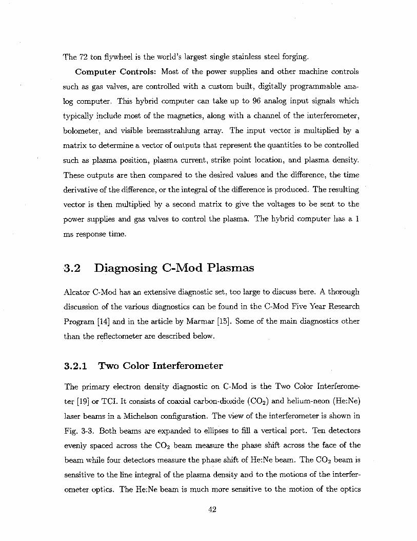
3.2.1 Two Color Interferometer
The primary electron density diagnostic on C-Mod is the Two Color Interferome-
ter [19] or TCI. It consists of coaxial carbon-dioxide (CC 2) and helium-neon (He:Ne)
laser beams in a Michelson configuration. The view of the interferometer is shown in
Fig. 3-3. Both beams are expanded to ellipses to fill a vertical port. Ten detectors
evenly spaced across the CO 2 beam measure the phase shift across the face of the
beam while four detectors measure the phase shift of He:Ne beam. The CC 2 beam is
sensitive to the line integral of the plasma density and to the motions of the interfer-
ometer optics. The He:Ne beam is much more sensitive to the motion of the optics
42
0.J
Po
Reflectometer
WR42OvermodedWaveguide
to
0
Itrferokmeter
Vacuum Vessel
Lal Limiter
Plasm
oi
msrotae 10
Stthfeldnes
Alcator C-Mod Density Diagnostics Cross sectionof the Alcator C-Mod device with all major density di-agnostics mapped to the same toroidal position. The RFprobe shown here is being replaced with a fast scanningprobe [16]. Also, an edge Thomson scattering diagnosticis under development in order to view the plasma nearthe X-point (17] along with a toroidally viewing interfer-ometer [18].
43
Figure 3-3:
H
and less sensitive to the plasma density than the CO 2 beam. Together these can be
used to separate the phase shift caused by vibrations and plasma. The line integrated
density measurements are typically good to 5 x 10¹⁸ M-3. Data from one channel is
available in real time for density feedback using the hybrid computer discussed in
@3.1.
The TCI has two limitations. First, the beam passes through a large portion of the
vacuum chamber above and below the main plasma. There can be a large inventory
of cold (> 10 ev), relatively dense (1019 to 1021 m-3) plasma in these regions. These
SOL plasmas are currently not measured or modeled sufficiently to separate edge and
main plasma contributions to the path integrated density measurements.
The second problem is the limited view port size. The small port size results in all
the TCI chords passing through both the edge and the core of the plasma. Fig. 3-4
shows the expected measurements for several different profiles which give identical
phase shift measurements on channel 4. Distinguishing between all but the most
extreme cases is not possible given the limited radial view. These limitations make
density gradient measurements unreliable, however the central density measured by
the TCI should be good to twenty percent in all but pellet fueled plasmas.
3.2.2 Core Nd:YAG Thomson Scattering
Another key density diagnostic is the Thomson Scattering System (TS). This is based
on a multipulse (50 Hz) Nd:YAG laser shining through a vertical port and viewed at up
to nineteen vertical positions1 through a horizontal port. Temperature measurements
are made by observing the doppler broadening of the laser light due to motion of
the electrons. Density measurements are made by observing the amplitude of the
scattered light. Properly calibrated, this diagnostic has the ability to make local
(2 cm resolution) measurements of the free electron density and temperature with,
usually, a five percent random error due to photon statistics. The challenges of
this diagnostic are maintaining alignment, reducing the stray light, and absolutely
f For the period during which the data for this thesis were taken, three or four channels wereoperating.
44

Density Profiles
E0
0
X
x
0.90
0.80
0.70
0.60
0.50
0.40
0.700.750.800.850.900.95Major Radius (m)
0 2 4 6 8 10Channel
Figure 3-4: Modeled TCI Measurements for several density pro-files. Note that the quite different profile shapes shownon the left result in nearly identical path length measure-ments on the right, making profile inversion difficult.
calibrating the device. While the signal to noise of the temperature measurement
depends on the absolute power and alignment of the beam, the Thomson scattering
temperature measurement is in general believed to be reliable. However the density
measurement depends directly on the amplitude of the light collected and is very
sensitive to alignment, changes in the collection optics, and efficiency of the detectors.
Calibration of the Thomson Scattering using the reflectometer will be discussed in
§ 6.4.4.
3.2.3 Probes
Lagmuir probes are used to measure edge plasma parameters at several locations
within the machine [20]. In the divertor, there are sixteen sets of three probes each
on the inner and outer divertor surfaces (see Fig. 3-5). In addition, there are probes on
the front faces of the limiters and a movable rf probe at A-port (the same port used by
45
4
E
0
x
I
0
nel
3 E
2 F

Fast-Scanning ProbeA
6
5Inner Probe
1Array 4
2 9 1
8
6
3 Outer ProbeArray
Figure 3-5: C-Mod DivertorLangmuir Probes
Including Fast Scanning and
46
k

*EFITD 33x33 04/21/95date ran = 2-JUN-95shot# = 950602024time (s)= 0.8000chi"2 = 16.6rout(cm) 67.680zout(cm)= -2.417a(cm) = 21.502elong = 1.604utriang = 0.372Itriang = 0.727indent = 0.000vol(cm3)= 8.76e+05energy(J)= 8.82e+04betat(%) = 0.637betap = 0.3281i 1.272error 0.000977q = 4.606qout = 6.944qpsib = 3.594dsep(cm) = 1240nmV/rc = 68.61/ 67.2zm//zc = 0.8// 0.6
data used:ip(kA) = -990.482btO(T) = -5.278
E
6k
'5
10
5
00.4 0.6 0.8 1.0 1.2
0.6
0.4
0.0
a
6
4
2
00.4 0.6 0.8 10 1.2
R(m)
-.0.2-
-0.4-
-0.6
0.40 0.50 0.60 0.70 0.80 0.90 1.00 110
Figure 3-6: Example EFIT Reconstruction
the reflectometer). Finally, a fast scanning probe can be fired vertically to the LCFS.
This probe generates edge temperature and density profiles with excellent spacial
resolution up to three times per shot. Currently it is limited to ohmic operation.
3.2.4 Magnetics and EFIT
The equilibrium fitting code EFIT [21] numerically solves the Grad-Shafranov equa-
tion based on inputs from the magnetics diagnostics [22]. Fig. 3-6 shows the curves
of constant flux as reconstructed by EFIT. Currently the only internal magnetic field
measurement is the tilt angle of the ablation cloud from injected lithium pellets [9].Such measurements are extremely perturbative and are not a part of normal opera-
tion. In addition no data from kinetic measurements are included. As a result, the
current profile determined by EFIT is parabolic. Comparison of the LCFS location
measured during L-mode by the divertor probes, the fast scanning probe, and EFIT
indicate that EFIT predicts the LCFS location to within 3 mm. The accuracy of
EFIT is less certain during H-modes and PEP modes as the current profile during
47
o'
0.6
0.4
0.2
0.0
-0.2
-0.4
-0.6
0.5 0.7 0.9 1 1R (m)
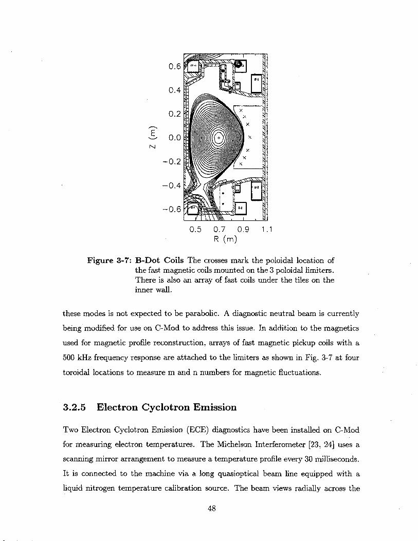
Figure 3-7: B-Dot Coils The crosses mark the poloidal location ofthe fast magnetic coils mounted on the 3 poloidal limiters.There is also an array of fast coils under the tiles on theinner wall.
these modes is not expected to be parabolic. A diagnostic neutral beam is currently
being modified for use on C-Mod to address this issue. In addition to the magnetics
used for magnetic profile reconstruction, arrays of fast magnetic pickup coils with a
500 kHz frequency response are attached to the limiters as shown in Fig. 3-7 at four
toroidal locations to measure m and n numbers for magnetic fluctuations.
3.2.5 Electron Cyclotron Emission
Two Electron Cyclotron Emission (ECE) diagnostics have been installed on C-Mod
for measuring electron temperatures. The Michelson Interferometer [23, 24] uses a
scanning mirror arrangement to measure a temperature profile every 30 milliseconds.
It is connected to the machine via a long quasioptical beam line equipped with a
liquid nitrogen temperature calibration source. The beam views radially across the
48

0.6
0.4
0.2
0.0
-0.2
-0.4
-0.6
0.
C-MOD H Aipha Views 960116027
N'.' toz
t
3 side
1.0R (rn)
=0.80
1 .5 2.0
Figure 3-8: Visible Diode Array Views [25] The views have beenmapped to the same toroidal location.
midplane with a spot size of - 3 cm in the poloidal direction. Attached to the same
beamline is a nine channel grating polychromator (GPC) which is cross calibrated
relative to the Michelson. The GPC has up to a 500 KHz frequency response and a
1.5 cm spacial and 9 eV thermal resolution. A third ECE diagnostic, a heterodyne
radiometer, is under development for diagnosing temperature fluctuations.
3.2.6 Spectroscopic Measurements
C-Mod has a host of spectrometers to study the line emission from the visible to the
X-ray. In addition, five imaging diode arrays [25] (shown in Fig. 3-8) image the D-a
emission and typically a carbon line. Four of the five arrays use Reticon linear diode
arrays and have 1 KHz frequency response. Top Array 1 has up to 1 MHz response for
viewing ELMs and hydrogen pellet ablation. Kurz [26] has combined the information
from all these arrays to perform tomographic reconstruction of the emission.
49
0.5
de

3.3 Major Areas of Physics Research
3.3.1 Transport Scaling
As discussed in §2.6, one of the most daunting problems facing plasma physics is
understanding energy transport in a tokamak sufficiently to be able to predict the
performance of a reactor. With its high magnetic field, high current density, and high
electron density, Alcator can explore a range of parameters that are complimentary to
what the rest of the fusion community can observe. For example, one important result
is the testing of neo-Alcator scaling in shaped plasmas. Studies on the circular Alcator
C tokamak produced the neo-Alcator scaling law [27] for the energy confinement time:
Tneo-Alcator = .166neR 2 -a-04o 5 .(3.1)
This strong dependence on ne and the lack of a dependence on Ip disagrees with the
ITER89-P scaling observed elsewhere:
TITER89-P = -048I0.85R 1 2a 0 3 n0 ' B0 2 amu p- (3.2)
On C-Mod, the ITER89-P scaling appears to be holding for significantly shaped
plasmas [28] adding confidence to its predictive qualities.
3.3.2 ICRF Heating
For many experiments on C-Mod, the 1 to 1.5 megawatts provided by ohmic heating
is sufficient. However, auxiliary heating is normally required in order to study plas-
mas with temperatures greater than 1 keV. Most large tokamaks use neutral beams
as their primary auxiliary heating scheme. However, the small ports and the long
port extensions on C-Mod allows only perpendicular launch of neutral beams. In
addition, the high plasma densities run on C-Mod make such beams impractical for
most current experiments. For Electron Cyclotron Resonance Heating (ECRH), C-
Mod would require sources above 140 GHz, but sources are not readily available.
50

Thus, Ion Cyclotron Resonance Heating (ICRH) is C-Mod's only auxiliary heating
sourceg. ICRH has the advantage of rugged and efficient sources and transmission
systems. The biggest challenge for ICRF heating is the limited surface power density
at the antenna and the generation of impurities due to RF sheaths formed between
the plasma and the antenna or between the wall and the antenna. Directly in front
of the antenna the launched waves are evanescent. A thicker evanescent region will
require larger fields at the antenna to couple a given power. The cutoff is located
where:
2 2
N2 = I + (3.3)11 WW" w(W+wci)
where nil = . kil is dictated by the geometry and phasing of the antennas. Substi-
tuting -= and solving for wp, gives:
w = (N - 1)(w + w)wd (3.4)
On C-Mod, Nil ~ 7, f = 80 MHz, and f6 ~ 29 MHz at the edge for a 5.3 tesla
on axis plasma. So the cut-off density is at ne ~ 7 x 10" in3 . This lies on the
outer edge of the SOL and is well below the lowest density monitored by the C-Mod
reflectometer. During L-H transitions, the location of this layer can move enough
to halve the loading on the antennas. Initially this posed a significant limitation on
heating during H-mode operation. ICRF heating puts several other restrictions on
plasma operation, in particular the choice of toroidal field, plasma shape, and plasma
composition.
Figure 3-9 shows the four straps of the two ICRF antennas currently in the ma-
chine. Each antenna is capable of launching two megawatts at 80 MHzh. To date,
the most successful heating results have been achieved at 5.3 tesla using a hydrogen
minority in a deuterium plasma. Up to 3.5 MW have been coupled in with an antenna
surface power density of 10 MW/m 2 . Successful ion heating has also been achieved
9 Lower hybrid heating and current drive are to be installed in 1997 or 1998.4Sources tunable from 40 to 80 MHz are currently being installed.
51
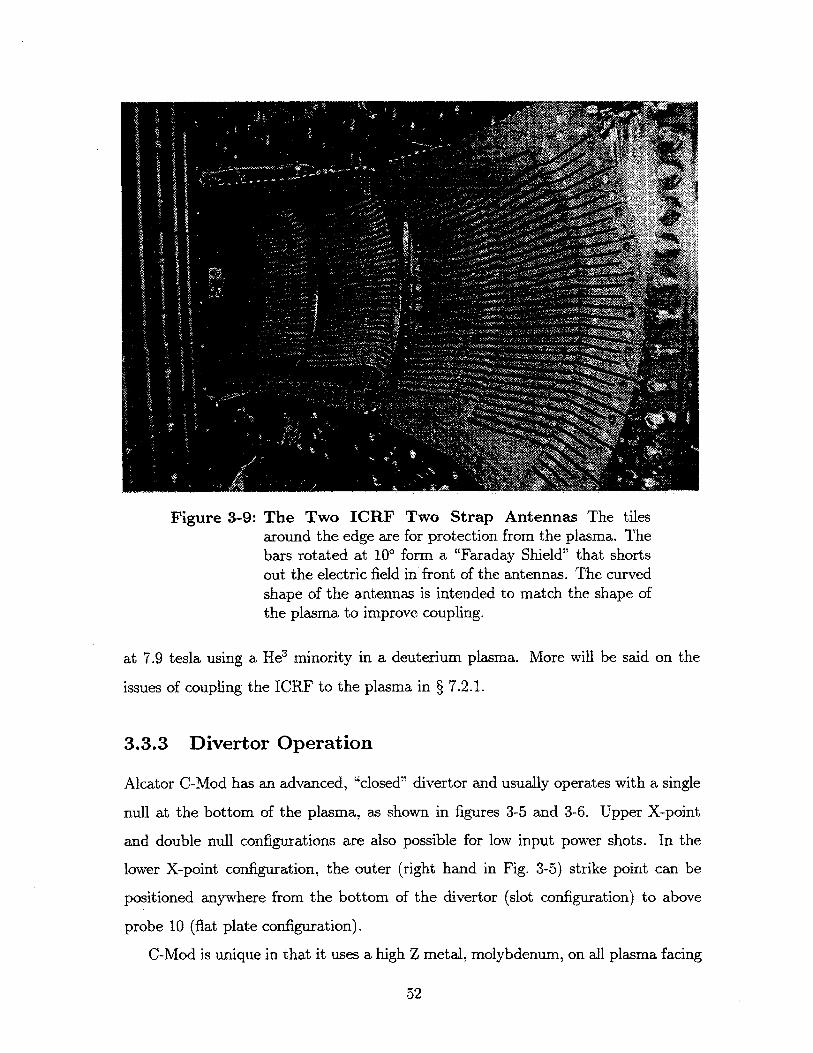
Figure 3-9: The Two ICRF Two Strap Antennas The tilesaround the edge are for protection from the plasma. Thebars rotated at 100 form a "Faraday Shield" that shortsout the electric field in front of the antennas. The curvedshape of the antennas is intended to match the shape ofthe plasma to improve coupling.
at 7.9 tesla using a He3 minority in a deuterium plasma. More will be said on the
issues of coupling the ICRF to the plasma in § 7.2.1.
3.3.3 Divertor Operation
Alcator C-Mod has an advanced, "closed" divertor and usually operates with a single
null at the bottom of the plasma, as shown in figures 3-5 and 3-6. Upper X-point
and double null configurations are also possible for low input power shots. In the
lower X-point configuration, the outer (right hand in Fig. 3-5) strike point can be
positioned anywhere from the bottom of the divertor (slot configuration) to above
probe 10 (flat plate configuration).
C-Mod is unique in that it uses a high Z metal, molybdenum, on all plasma facing
52
surfaces . Most tokamaks use carbon. More than 8000 molybdenum tiles cover much
of the inside of the C-Mod vacuum chamber. The small rectangles shown in Fig. 3-3
along the bottom, inner cylinder, and top of the vacuum vessel indicate the surfaces
covered by tiles. The limiter between ports A and B and the two limiters on either
side of port G are also covered by molybdenum tiles.
During L-mode operation, the density can be controlled well via gas puffing, unlike
a carbon walled machine. After major disruptions, the next plasma attempt usually
succeeds though a "fizzle" or short low current plasma may result instead. One fizzle
usually conditions the walls sufficiently to obtain a plasma on the second attempti.
Both of these results are attributed to the molybdenum walls. Unfortunately, the
radiated power in C-Mod prior to wall conditioning with boron is very high, often
over 50%.
The C-Mod divertor has three modes of operation [20, 29]: sheath limited, high
recycling, and detached. In the sheath limited regime, the electron temperature and
pressure is conserved along a field line. In the high recycling regime, pressure is
conserved on a field line, but temperature is not. And in the detached regime, both
electron pressure and temperature are not conserved. Detachment has only been
observed with electron temperatures of 6 eV or less.
3.3.4 Improved Confinement Modes
Both PEP and H-modes have been achieved in C-Mod. The PEP modes provided
very peaked density profiles with central densities greater than 1.2 x 10²¹ m 3 . The
thesis by Ganier [9] reviews the PEP results.
An excellent review of H-mode studies on C-Mod can be found in Greenwald [30,
31]. H-modes have been achieved on C-Mod in ohmic and ICRF heated plasmas but
only in diverted operationk. Alcator C-Mod is normally run with the ion B x VB drift
A plasma facing surface is any spot on the machine that can be touched by hot plasma eitherduring normal operation or during a disruption.
3 The vacuum vessel walls can be further conditioned by electron cyclotron discharge cleaning,glow discharge cleaning, lithiumization via pellet injection, and boronization.
kVery little run time has been devoted to high power limited plasmas, so the ability to obtainlimited H-modes is not precluded.
53
directed towards the divertor (down). This is the favorable direction for obtaining H-
modes. A small number of H-modes has been achieved with the B x VB drift in the
opposite direction and required twice the power needed for obtaining H-mode with the
favorably directed drift. This increased power threshold may be due to the reduced
power delivered to the outer strike point in reversed field operation. This reduced
power makes the outer strike point significantly colder and often detached. As a result
the pumping effectiveness of the divertor is reduced. Typically, the compression ratio
is half that achieved with the B x VB drift down. However, main chamber pressures
are within the range for which H-modes would be expected in normal operation.
The characteristics of the various manifestations of the H-mode in C-Mod and the
variation with respect to surface conditions will be discussed further in § 7.
54
Chapter 4
Reflectometry Theory
In this chapter, a rather basic discussion of the theory of reflectometry will be pre-
sented. It should be noted that the understanding of the effect of fluctuations on the
returned signal from a reflectometer is an area of continued research and is beyond
the scope of this thesis. The interested reader is referred to the occasional IAEA
meeting on reflectometry [32, 331 for the latest theories.
4.1 Dispersion Relations
Krall and Trivelpiece [34] derive the dispersion relations for an electromagnetic wave
propagating in a cold, stationary, collisionless, homogeneous plasma. The derivation
will be briefly outlined here using their notation. The magnetic field is chosen to be
in the z direction and the wave is assumed to be traveling in the y-z plane at some
angle 0 relative to B (see Fig. 4-1). The perturbed quantities of the wave, E1 , B1 , vil,
and ni, are assumed to have a spatial and temporal form of:
E1(r, t) = $1 (k,w) exp(i(k - r - wt)]. (4.1)
By applying Maxwell's equations, along with continuity and m = q(E + v x B), a
matrix relation for the electric fields is derived. In the limit of frequencies far above
55
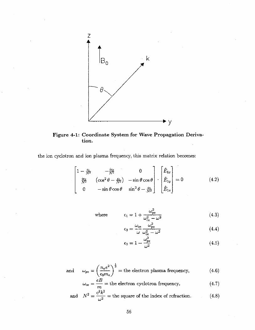
z
BO k
0
Figure 4-1: Coordinate System for Wave Propagation Deriva-tion.
the ion cyclotron and ion plasma frequency, this matrix relation becomes:
I1 0 [ 1 1N 2- [E12
N2 o N2 sin 0 cos 0 - 0 (4.2)
0 - sin 0cos 0 sin 26 -0 1j
L Nw2 J- L
2where EW 1 + 2e (4.3)
W2 --W2____ oCe
E 3 1- W-- (4.5)w2
1e
and 1 = (*,2 - the electron plasma frequency, (4.6)
eB= = the electron cyclotron frequency, (4.7)
mc2 k 2
and N 2 2 = the square of the index of refraction. (4.8)
56
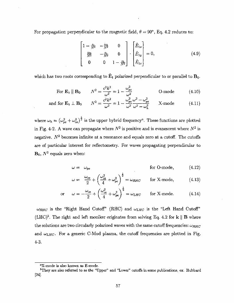
For propagation perpendicular to the magnetic field, 0 = 900, Eq. 4.2 reduces to:
1 §-I_ -Lea 0 Ei.
.LE - 0 -E =0, (4.9)
0 0 1 - E3 12
which has two roots corresponding to E1 polarized perpendicular to or parallel to BO.
For E1 |1 Bo N 2 = c2k 2 WP 0-mode (4.10)
c2 k2 "2 w2 _ ,2
and for E 1l Bo N 2 =- 2 _ W _ e X-mode (4.11)W2 w 2 2 -O 2
LO h
where Wh = (w, + w2,)2 is the upper hybrid frequencya. These functions are plotted
in Fig. 4-2. A wave can propagate where N 2 is positive and is evanescent where N 2 is
negative. N 2 becomes infinite at a resonance and equals zero at a cutoff. The cutoffs
are of particular interest for reflectometry. For waves propagating perpendicular to
Bo, N 2 equals zero when:
W =We for O-mode, (4.12)
W + + w+2) =WPJC for X-mode, (4.13)
Wce (W C L2\or W-= - + + P) WLHC for X-mode. (4.14)
wpJIc is the "Right Hand Cutoff" (RHC) and wLuc is the "Left Hand Cutoff"
(LHC)b. The right and left moniker originates from solving Eq. 4.2 for k H1 B where
the solutions are two circularly polarized waves with the same cutoff frequencies: wpIC
and WLHC. For a generic C-Mod plasma, the cutoff frequencies are plotted in Fig.
4-3.
'X-mode is also known as E-mode.'They are also referred to as the "Upper" and "Lower" cutoffs in some publications, ex. Hubbard
[24].
57

0 Mode Cutoff4
2
-2
-4
4
2
-24
X o o (epe
X Mode Cutoffs (W-c =Wr
C- JLHC () )RHC
0.6 0.8 1.0 1.2 1.4 1.6 1.8 2.0W/Wpe
Figure 4-2: 0 and X Mode Reflection Above are plotted the dis-persion relations for perpendicular propagation for the 0and X mode for a cold plasma assuming stationary ions.In the shaded regions the waves are evanescent.
4.2 Accessibility in Toroidal Geometry
The first requirement for the application of the cutoffs discussed in § 4.1 to tokamak
plasma diagnosis is determining where the plasma can be probed with a given fre-
quency. To aid in this, the mapping of the cutoffs to major radius-density space will
be presented. For the O-mode, this mapping is quite simple and is shown in Fig. 4-4.
The cutoff frequency, f,, is proportional to the square root of the electron density
and independent of B. The first intersection from the right of the density profile with
each of the horizontal curves is where that particular frequency will reflect. For mod-
erately hot plasmas, absorption at the first harmonic can prevent access to the cutoff.
The total magnetic field in a tokamak falls off approximately as 1/r for low 3 plasmas
giving the hyperbolic curve where f, = fp,. Low field launched 0-mode waves can
not pass this curve. For example, 125 GHz launched from the low field side would
not reach the cutoff for the density profile shown, as the resonance at 0.8 meters will
absorb the launched wave. Frequencies below 105 GHz should be unaffected, as the
58
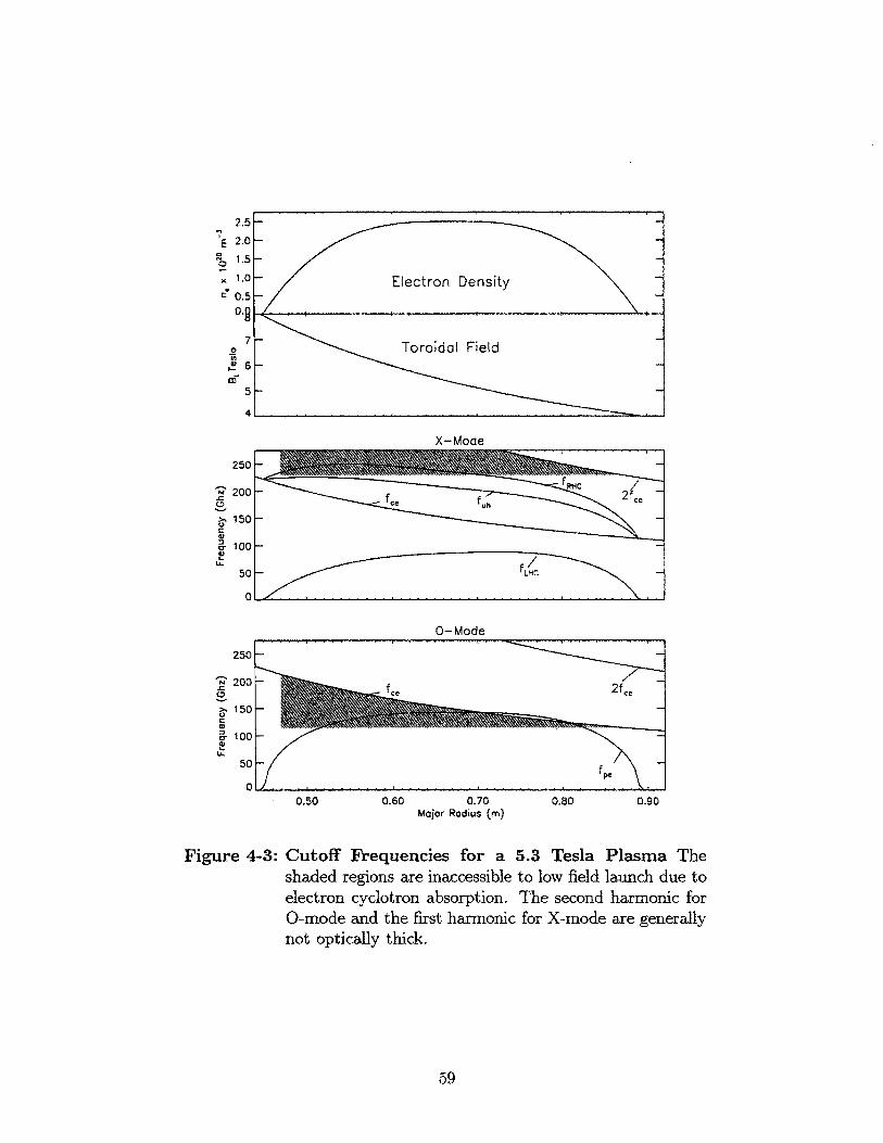
2.5-
2.0-
1.5-
1.0- Electron Density0.5-0.0
S ~Toroidal Field6 -
5 -
X-Mode
RHC 2
fL /
0-Mode
0.50 0.60 0.70Major Radius (m)
Figure 4-3: Cutoff Frequencies for a 5.3 Tesla Plasma Theshaded regions are inaccessible to low field launch due toelectron cyclotron absorption. The second harmonic for0-mode and the first harmonic for X-mode are generallynot optically thick.
59
E
0
I..
a
250
2 200
150
100
50
0
C,
0
0-
fc -ceCe ce
0-
0-
0
0.80 0.90
4
25
20
15
10
5
6tpe= f2ce.
200'U
E4-E 175ce pe
(NN
150x
S2 ------ --------- 125
100L xample Density Profile
eF50
0 500.4 0.6 0.8 1.0
Major Radius (M)
Figure 4-4: 0-Mode Accessibility Plot for 5.3 Tesla An exampledensity profile is included. On C-Mod the inner wall is at0.44 meters and the limiters are at .905 meters. Typicallythe LCFS is at .89 meters and the plasma magnetic axisis at .68 meters.
edge plasma is too cold and tenuous at the location of their cyclotron resonance to
have a significant optical depth.
The O-mode case is simple compared with the X-mode case shown in Fig. 4-5.
Here the curve f, = fp, is included along with the right hand axis from Fig. 4-4, so
0 and X mode access can be compared. Equation 4.13 can be solved for fpe,c,it as a
function of launched frequency, f, and radius, r:
ft(f, r) = (f - f(r)) f r) (4.15)
Then, using B(r) = Bo0 and Eq. 4.6, nci as a function of r can be specified. The
curves labeled on the right of Fig. 4-5 correspond to the critical densities for the
RHC from 120 to 300 GHz. Above about 210 MHz, absorption at f = 2f, becomes
important. Substituting this condition into Eq. 4.15 gives the curve fp, = v'2fe on
which the access curves from 240 to 300 terminate. The ECE diagnostics observe
60
A

6 14'
\ 260 N120' ~ .20 200
f--240 175
\f- -fe
0 _\ce pe .-220 (D
108001 50
140 10 --10-
~ ~- -- - -- 12 O 5 00-
0.4 0.6 0.8 1.0Major Radius (m)
Figure 4-5: Accessibility Plot for 5.3 Tesla The values 20 to 140on the left correspond to the curves demarking the criticaldensities for 20 to 140 GHz for the LHC. The numbers120 to 300 on the right do the same for frequencies 120to 140 GHz for the RHC.
emission in this range of frequencies. A density profile that cuts through these curves
will cut off the ECE emission, giving a potentially very accurate density measurement
at the expense of a temperature measurement.
The curves labeled at the left of Fig. 4-5 correspond to the LHC. Using the same
analysis in Eq. 4.14 results in:
fp2ecrit() = (f 2 + f. 2 (r) (4.16)
In order to be launched from the low field side of the tokamak and reach the LHC, the
launched wave must at some point pass through the RHC/upper hybrid resonance
pair. This can be seen in Fig. 4-2. In a tokamak diagnostic, the plasma density near
the horns is low and gets higher as the launched waves approach the plasma center.
On Fig. 4-2 this corresponds to moving from right to left. If the density is zero where
f = fe, then the resonance and the cutoff are in the same place and the launched
61
6
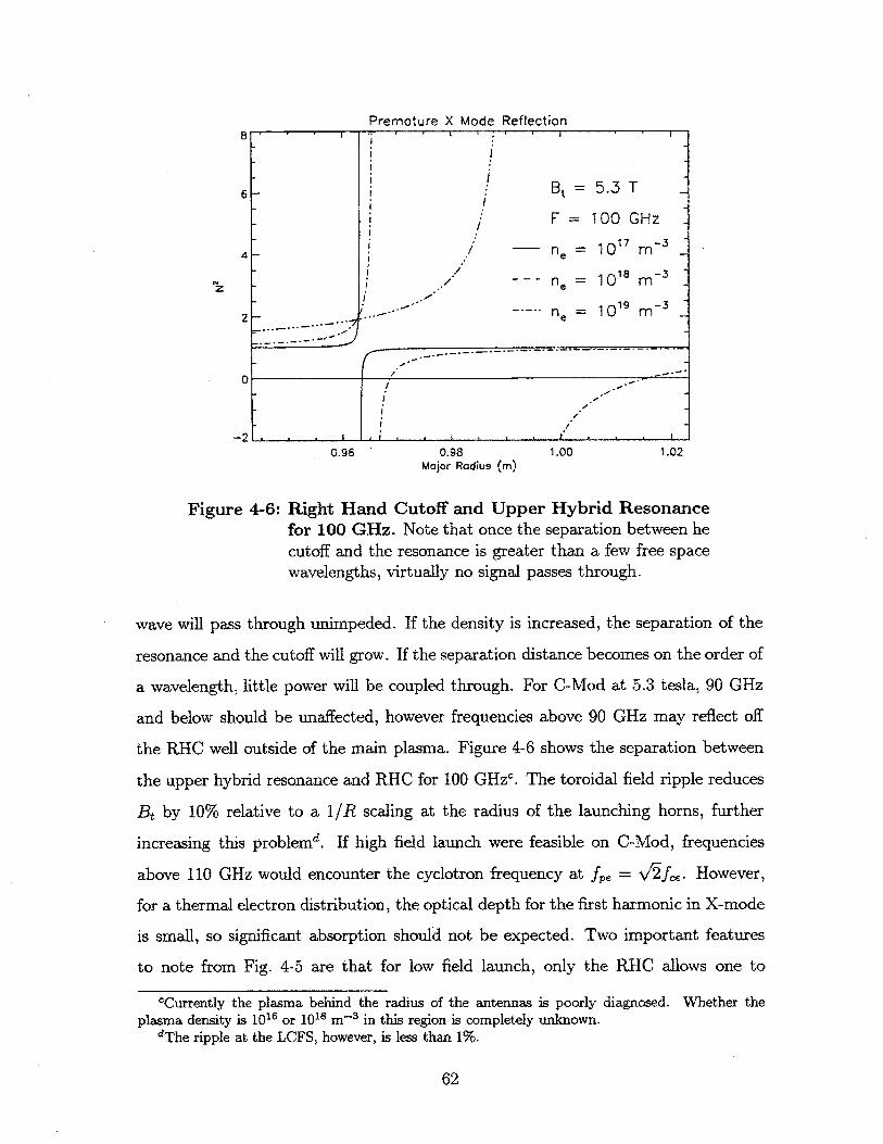
Premature X Mode Reflection
6 Bt 5.3 T
F =100 GHz
'17 -3-- ne 10 m
z- =
2 ..- -- ne 10 m~3
0.96 0.98 1.00 1.02Major Radius (m)
Figure 4-6: Right Hand Cutoff and Upper Hybrid Resonancefor 100 GHz. Note that once the separation between he
cutoff and the resonance is greater than a few free spacewavelengths, virtually no signal passes through.
wave will pass through unimpeded. If the density is increased, the separation of the
resonance and the cutoff will grow. If the separation distance becomes on the order of
a wavelength, little power will be coupled through. For C-Mod at 5.3 tesla, 90 GHz
and below should be unaffected, however frequencies above 90 GHz may reflect off
the RHC well outside of the main plasma. Figure 4-6 shows the separation between
the upper hybrid resonance and RHC for 100 GHzc. The toroidal field ripple reduces
Bt by 10% relative to a 1/R scaling at the radius of the launching horns, further
increasing this problem'. If high field launch were feasible on C-Mod, frequencies
above 110 GHz would encounter the cyclotron frequency at f, = v'/f,. However,
for a thermal electron distribution, the optical depth for the first harmonic in X-mode
is small, so significant absorption should not be expected. Two important features
to note from Fig. 4-5 are that for low field launch, only the RHC allows one to
currently the plasma behind the radius of the antennas is poorly diagnosed. Whether theplasma density is 1016 or 1018 m-3 in this region is completely unknown.
dThe ripple at the LCFS, however, is less than 1%.
62

140 340 250- -320
120 ]
f 6 -300 225
E 100 U.28C 200 C
0
48 .. 261175 '
6 0 -- 2 4 0 1 5
-- 2202 40 e . - 125 E- 200 (n
- - 100020- --,--- 180 m0- -- - ~------16 95
./' -~ '-50
0.4 0.6 0.8 1.0Major Radius (m)
Figure 4-7: Accessibility Plot for 7.9 Tesla (see Fig. 4-5 for label-ing scheme.
study hollow profiles, while the LHC allows one to study a given density with a lower
frequency using generally less expensive sources and detectors. Figure 4-7 shows the
same accessibility plot for 7.9 tesla. At this field, frequencies above 140 GHz will
suffer the same access problems in reaching the LHC as was discussed for frequencies
above 90 GHz at 5.3 tesla.
4.3 Wave Propagation in a Stratified Medium
In this section the propagation of 0-mode waves through an inhomogeneous medium
will be discussed. Much of the material, including the notation, is extracted from
Ginzberg [35] chapter 4. The particular condition to be discussed is k 11 Vne, k I BO,
and, of course, E1 11 Bo. The wave equation for these conditions is:
d2PIZ(Y) + 2
y2 + 2 C(L, y)k12(y) = 0. (4.17)
63
For clarity and to make the author's life easier, E will be substituted for ti,(y) for the
remainder of this section. First, a linear density profile for which the wave equation
can be solved exactly will be presented. Equation 4.17 has the same form as the time
independent Schroedinger Equation':
d0 2md2 )+ 2m (E - V(y)) =0. (4.18)
The WKB method commonly used to solve Eq. 4.18 will be discussed and finally an
"Abel like" inversion of reflectometer data to give density profiles will be presented.
4.3.1 Exact Solution for Linear Density Profile
For 0-mode propagation perpendicular to the magnetic field with a linear density
profile, an exact solution can be obtained. Inserting
n,(z) = n, -, n(y1 ) = n, = the critical density for w, and E = 1 .Y1 y1
into Eq. 4.17 and making the substitution:
2 )1/3 (WJ2/36(=((y -y = - y (4.19)
reduces Eq. 4.17 to:
d2E+ CE =0. (4.20)
Equation 4.20 has solutions of the form of Bessel functions with the boundary condi-
tion that E -+ 0 as y -+ oo (or C -+ -oc).
E(C) = A(1 2 (J113 (3 ) + J-1 1 3 (p3/2 for C > 0 (4.21)
E(C) = A(-() (-11/3 (3 /2 + 1- 1 3 ( (_)3/2 for C < 0, (4.22)
'All those classes amount to one line in my thesis!
64
or the Airy integral:
E(C) = cos - (x dx. (4.23)
For ( > 1, i.e. for y many wavelengths from the reflecting layer, Eq. 4.23 reduces to:
E(() _ (-1/4 cos (3/2 - (4.24)
The fields calculated here are for a standing wave with one wave travelling in and
one travelling out. This can be seen most clearly by including the time dependent
portion of E. The real portion of the electric field, '((, t), is simply:
t)= E cos[w(t - to)] (4.25)
A 2o/ cos (2r3/2 _ _r w(t _ to)] + cos [ (3/2 - + O(t - to)
(4.26)
The first term on the right corresponds to a wave moving in the +( or -y direction.
The term on the left is a wave moving in the -( or +y direction. With a little algebra,
a portion of the argument of the cosines above can be written in a very suggestive
form:
2(3/2 2] (YI _ Y)3/2 _ 7 (4.27)3 4 3coy 124
/2 (y - y')41 2dy' - (4.28)C 1 . 1
= j N(y')dy' - (4.29)
= f'i k(y')dy' - (4.30)Jy 4
65
Now choosing to so that the phase of the wave going in the positive y direction at
some point y" is zero at t = 0, we get:
(y", t) K cos wt -- [] N(y')dy' - -) + Kcos(wt), (4.31)
where:
3A 3A 2rrcK 3 - and, Ao =- (4.32)
2/7(/4 2 ( 274 Y)1/6 N (y) 4O
So the phase difference between the launched and reflected waves for a linear profile
equals the integral of the local index of refraction along the path travelled by the
wave times 21 minus a ' correction.
4.3.2 The W.K.B. Method
Key to the application of reflectometry is the approximation of "Geometrical Optics"
or the "W.K.B. method"J. The approximation of geometrical optics is that the
wavelength of E.M. radiation at a given location can be determined by the local
index of refraction. Also, the power reflected from a gradient in the index is small.
Again Ginzberg [35] gives a rigorous derivation of the approximation of geometrical
optics. Dicke and Wittke [37] do the same for the quantum mechanical analog. The
derivation will not be repeated here other than to say a function of the form:
E(y) = Eo(y)e- !- 1(Y) and 0(y) = t N(y)dy (4.33)
fIt should be noted that while Wentzel, Kramers and Brillouin each independently in 1926 andJeffreys in 1924 applied this technique to wave mechanics, Gans used them to study radio waves inthe ionosphere in 1915 and Lord Rayleigh used them to study sound waves in 1912 [36]. The valueof working in a popular field is evident.
66

is inserted into Eq. 4.17 and ordered in terms of '. Eo(y) is assumed to vary slowly
with respect to A and yo is an arbitrary constant. After some algebra the result,
E ) C+ + f' N(y)dy C- -iE- f_ N(y)dyE(y) e CN0(y) e ± Nf() (4.34)
N (y) NI(y)
is found, where the + and - represent waves propagating in the +y and -y directions.
This approximate solution holds provided:
dN
Ao dy «1N2 < 1.(4.35)
The W.K.B. approximations fail near a reflection. The phase for a linear profile has
been calculated above. If the profile is assumed to be linear near the reflecting layer,
a correction of - 2 to the phase is applied. Multiplying the total phase shift by two
for propagation into and out of the plasma, we get:
2w a 7r
() = - N(y)dy - -. (4.36)
The steepest density gradient expected in the main C-Mod plasma will occur in the
SGR of an ELM free H-mode. The expected lower limit for the scrape off length, ISOL,
in the SGR is the ion banana orbit width ~ 2mm. Assuming ne = n exp(-y/.002)
where n, is the critical density for f. For an exponential density profile relation 4.35
reduces to:
Al < N = 1 - (f (4.37)
For wavelengths from .6 to .27 cm (50 to 110 GHz) and assuming IsoL ~ .002 meters,
WKB theory holds for g < 0.7. This is not a problem as long as the gradient
continues to the critical density. However, if the profile has a kink in it as shown in
Fig. 4-8, a significant reflection can occur at the steep gradient.
67
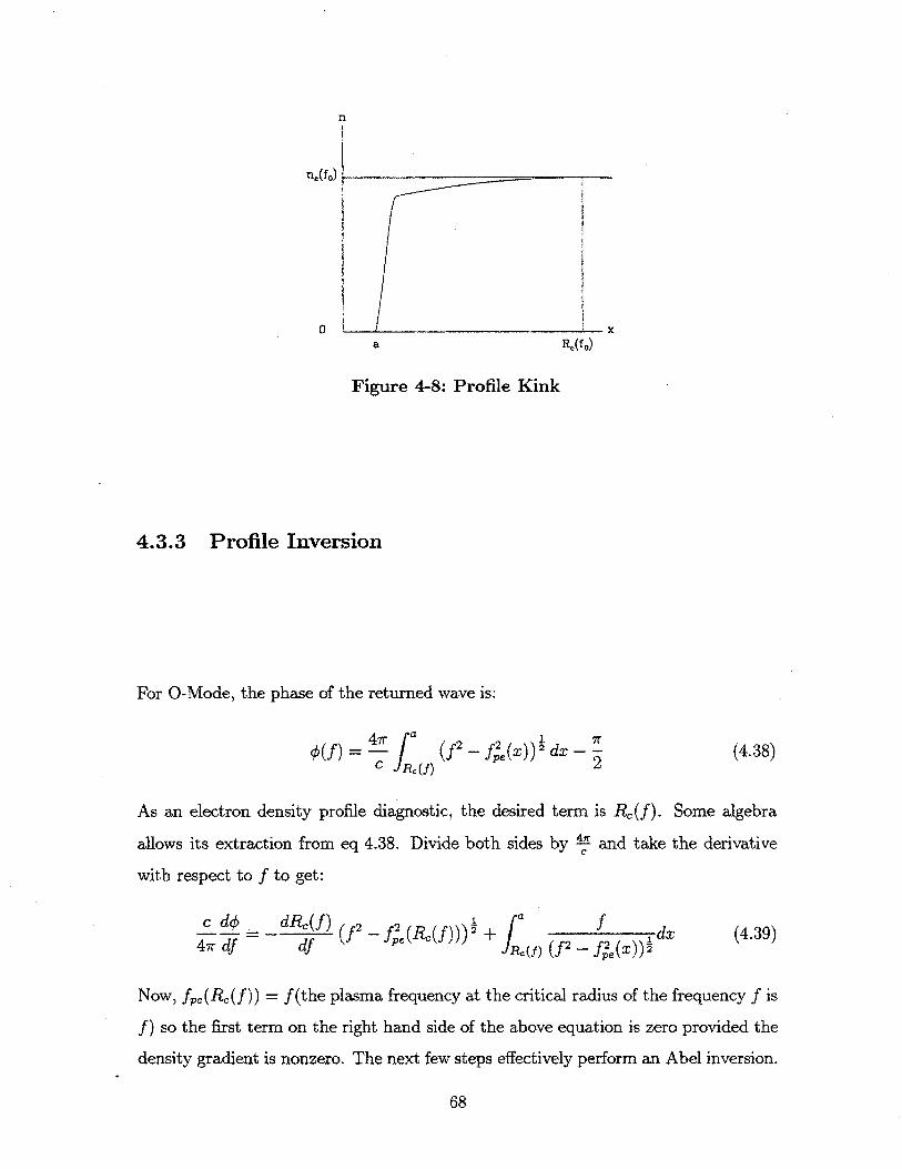
n
n.(f.)
0a
Figure 4-8: Profile Kink
4.3.3 Profile Inversion
For O-Mode, the phase of the returned wave is:
() = 4I(fC JR.U)
(f2_f (X)) dx -(4.38)
As an electron density profile diagnostic, the desired term is R,(f). Some algebra
allows its extraction from eq 4.38. Divide both sides by ' and take the derivativeC
with respect to f to get:
S =d _ dRC(f) [a f47r df df + J (f 2 - f2e()) 1 (4.39)
Now, fpe(Rc(f)) = f(the plasma frequency at the critical radius of the frequency f is
f) so the first term on the right hand side of the above equation is zero provided the
density gradient is nonzero. The next few steps effectively perform an Abel inversion.
68
xR.(f0 )
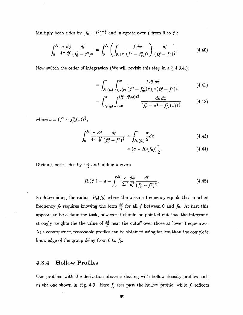
Multiply both sides by (fo - f2) - and integrate over f from 0 to fo:
fo c do5 df fo( " f dx df (440)4irdf (f-f2)? - Jw(f2 -f2) (f2 -f2)
Now switch the order of integration (We will revisit this step in a § 4.3.4.):
a ff0ffd=f' f" x(4.41)
=IRe(fo) Ie(x) (f2 - f(X)) )(f2 _ f2);
a (f.2f (X))2 dudx (4.42)R4(fo> =_ (f -- 2 - fe (x)) 12
where u = (f2 _ (X)) ,
Sfoc do df (4.43)
o 47 df (f2 -- f2)3 J&(f) 2
= (a - R,(fo)) . (4.44)
Dividing both sides by -2 and adding a gives:
Re(fo) =a-f f c do df (4.45)10 2 7r2 df (f02 - f 2)2
So determining the radius, R,(fo) where the plasma frequency equals the launched
frequency fo requires knowing the term 0 for all f between 0 and fo. At first this
appears to be a daunting task, however it should be pointed out that the integrand
strongly weights the the value of ! near the cutoff over those at lower frequencies.
As a consequence, reasonable profiles can be obtained using far less than the complete
knowledge of the group delay from 0 to fo.
4.3.4 Hollow Profiles
One problem with the derivation above is dealing with hollow density profiles such
as the one shown in Fig. 4-9. Here f3 sees past the hollow profile, while fi reflects
69
fo n
fj
fi
a Rc(fo)
Figure 4-9: Hollow Profile Inversion Problems
before the hollow portion. The group delay observed by fj does not contain enough
information to reconstruct the profile of the hollow region. In the derivation above,
the problem arises in going from Eq. 4.40 to Eq. 4.41 by switching the order of
integration. This is only allowed if f and R, are one to one. Figure 4-10 plots R,(f)
and shows the difference in the two regions of integration. The horizontal lines in the
left hand figure are the paths for the first integration in Eq. 4.40 which omit a portion
of the hollow region. The figure on the right hand side shows the integration region
for Eq. 4.41. The first integration follows the vertical paths shown. The result of a
hollow profile will be an underestimation of the distance from "a" to the reflecting
layer. While it may appear possible to reconstruct some of the hollowness for the
particular case shown through an iterative approach and some smoothing procedure,
in practice, the noise in each measurement and the fluctuation in the density at the
local maximum and minimum between the cutoffs for f, and f3, make such analysis
impractical.
70

i xa RefO)
f
Figure 4-10: Integration Paths
4.4 Plasma Absorption and Emission
Hutchinson [38] derives the optical depth r for single pass for the 0-mode at an
arbitrary angle. For the specific case of perpendicular propagation his result reduces
to:
La /2 TWcer- where, a=2-w e(1- and L= -=R
WCC 2c MC, mec
ds
(4.46)
where R is machine major radius. The cyclotron resonance for 110 GHz is at 90 cm for
5.3 Tesla operation. This is typically in the SOL with ne < 1020 m-3 and Te < 100 eV
giving a maximum optical depth of .3 for a single pass or .6 for a return path. This
has not appeared to adversely affect operation. For the rest of the frequencies used
the cyclotron resonance is well outside the main plasma. When operating at lower
field absorption has limited access.
Emission of radiation in the frequency bands used can be an issue. If the plasma
71
f
fo
0 xa R.(fo)
fo
0

density is low enough, runaway electrons can be presents. The runaways are very
relativistic, thus reducing their emission frequency by the ratio of their rest mass to
their relativistic mass. So the reflectometer can observe emission from these electrons
despite the nominal cyclotron resonance being much higher. Large bursts of emission
can often be seen often coinciding with sawtooth crashes. The bursts could be due to
runaway electrons being kicked out of the center of the plasma where their emission
was cutoff or having some of their parallel momentum converted to perpendicular
momentum by the sawtooth crash, again causing their emission to be seen. Previous
work on Alcator C has demonstrated the existence of a cyclotron maser [39] effect. On
one occasion, a C-Mod reflectometer mixer failed during a shot with a high runaway
population. High plasma emission or X-rays from fast electrons hitting machine walls
are assumed to be the cause. Reflectometers on other machines have experienced
failures due to unknown causes [40, 41]. Emission from runaways may be the culprit.
4.5 Relativistic Effects
Binslev [42] has worked out relativistic corrections to the cutoffs for reflectometry.
For a given 0-mode reflectometer frequency, the relativistic cutoff density, nerd, will
be slightly higher than the density, necoid, calculated from cold plasma theory. For
temperatures below 20 keV the correction factor to five significant digits is:
* r = vo ~ + 4.892 x 10⁻³ V 2.24 x 10~6ne cio j \keV kV
+ 2.3 x 10~" (e) (4.47)
9The collision frequency between particles in a plasma drops as their velocity increases. Runawaysare electrons that have been accelerated by the ohmic current drive to velocities where the drag dueto collisions is small compared to the accelerating potential. Such electrons can reach energies inthe 10's of MeV's.
72
and the relativistic index of refraction No is
f2 .N,, ~- 2 (4.48)
For almost all our current operating conditions, Te is less than 4 keV, giving vo <5 1.02.
This is small compared to the other errors in our measurements, however this could
become an issue in the future as heating power and confinement times increase. In
particular, cross calibration of the Thomson Scattering system based on reflectometer
cutoff (see § 6.4.4) should not be attempted on ICRF heated shots.
73
74
Chapter 5
The Alcator C-Mod Reflectometer
In this chapter the hardware and rf techniques used for the C-Mod Reflectometer will
be described.
5.1 Design Philosophy
At the time this project was being developed, reflectometry had met with limited
success [43, 24, 44, 45, 46, 47]. In order to apply Eq. 4.45, most experiments required
that the phase of the returned signal be monitored as the launched frequency was
swept over either a broad or narrow range. If at any point the returned signal dis-
appeared or gained too much noise, the do term would pick up a modulo 27r error.
The difficulty in following the phase of the returned wave over the long periods of the
source sweep would compromise these diagnostics.
Hubbard, Prentice, and Sips from the Joint European Tokamak (JET) provided
much useful advice on the specific difficulties they encountered with their reflec-
tometer. Two issues that had been particularly challenging to the JET group were
combining multiple frequency bands into one transmission and receiving line, and
dealing with the complicated mode structure of their long, overmoded transmission
line with multiple bends. C-Mod has the good fortune of comparatively easy access
to the machine, and few of the radiation shielding requirements of the JET program.
The diagnostic at A-port was arranged so that few bends in the waveguide runs
75

would be needed, and so it would not be necessary to be greatly overmoded. Also,
each waveguide band was given a separate pair of horns. Additionally, this diagnostic
was considered an experimental diagnostic subject to major reconfiguration. Further,
connectorized components built to designated specifications for all rf circuit boards
operating at more than 30 MHz were purchased, allowing the designers/builders of
this diagnostic to expend and develop their expertise elsewhere.
5.2 Differential Phase or AM Reflectometry
Sufficient progress has been made in reflectometry so that it can now be proposed
as a core electron density diagnostic for fusion research plasmas [48]. Key to this
progress has been the development of alternative modulation techniques. "Differential
Phase" (DP) or "Amplitude Modulated" (AM) reflectometry has become a common
diagnostic technique [49, 50, 51, 52, 53]. This approach was first suggested by Rich
Chedester of Millitech Corporation. It was first proposed as a plasma diagnostic on
C-Mod in 1990 [54].
Figure 5-1 shows the fundamental idea behind DP reflectometry. Instead of mea-
suring the change in phase as one sweeps the frequency, one launches two closely
spaced frequencies and measures the phase difference of the returned waves.
Launched signal: sin[27r(F + AF)t] + sin[27r(F - AF)t]
Received signal: sin[27r(F + AF)t - 41+ sin[27r(F - AF)t - 02]
OW =47r 2 PC () = (f2 _ 2)2 dx - (51)
In the detector the two signals are mixed and the low frequency term is:
sin[27r(F + AF)t - 01 - (27r(F - AF)t - 02)] = sin[47rzAFt - AO]
where, A4 = 41 - 02
76

Crystal Oscillator(500 Mhz)
AFDoubler To Plasma
isolator F+AF, F-AF
F
Gunn Oscillator Detector(50-110 Ghz)
From PlasmaF+AF, 01
A sin(4nAF +Ao) F-AF, o2
B sin(47cAF)
iPhaseDetector
sin(Ao) cos (Ao)
a
ne
Figure 5-1: AM Technique A4 = 01 - 02
The group delay for the beat wave to travel to the reflecting layer and back is:
r = 41rAF (5.2)
As long as AF < F- and the density profile does not have a major break in slope at
ne = nc(F), then 7. is independent of AF. Then AF can be chosen such that the
expected range of A4 is less than 27r so there is no ' ambiguity in rg. For example,
if the group delay from the launching horns to the critical layer can range from 1
to 2 ns (corresponding to an optical path from 30 to 60 cm), then AF ; 500MHz.
Higher frequencies will give better phase resolution provided the separation distance
between the two reflecting layers is small relative to the turbulence corelation length.
Another popular approach to making profile measurements with reflectometry is
to use an electronically swept oscillator and monitor the returned phase or returned
77

frequency as the source is swept over either a narrow (100 MHz to 1 GHz) or broad
(one waveguide band) range. The advantages and disadvantages of a fixed-frequency,
multi-channel DP reflectometer as developed for C-Mod compared to such swept
systems are:
Advantages:
" No frequency modulation needed. This reduces some of the complexity of
the system.
" No 2nr ambiguity in the returned phase. By choosing AF small enough,
as discussed above, temporary loss of signal due to plasma turbulence does not
result in an ambiguity in the returned phase. Systems that depend on following
the phase of the returned signal during a frequency sweep can "lose fringes".
" Time response dictated by output filtering rather than sweep rate.
The integration time over which a measurement is made can be made as short
or as long as desired.
" Simplified transmission system. The performance of a fixed frequency DP
reflectometer is completely independent of the mode structure of the transmis-
sion line provided the isolation between the launching line and the receiving line
is high. In a swept system, multiple reflections in the transmission lines must
kept small or somehow calibrated out.
" No reference leg is needed. A swept system requires a reference arm. This
can be a major or minor detail depending on the distance from the source to
the launching antennas and the modulation technique.
" Automatic frequency stabilization. All drifts in the millimeter wave oscil-
lators are mixed out in a DP reflectometer receiver. The phase information is
carried on the 2AF beat wave which can be provided by a very stable crystal
oscillator.
Disadvantages:
78
" Sensitive to multiple reflections. Multiple reflections in the vacuum cham-
ber during plasma operation or during calibration will corrupt signals in a DP
reflectometer. A fast swept system can in principle distinguish between re-
flections from the plasma and multiple reflections inside the chamber. To ac-
complish this the launched frequency must be swept fast enough so that the
expected returned frequency offset range is large compared to the broadening
expected from fluctuations, and the expected range of returned frequencies from
a plasma reflection must not overlap the range for multiple reflections.
" More complicated fluctuation analysis. The returned fluctuation signal
from a DP reflectometer will be the product of the scattering of the two launched
frequencies. To date, high frequency data have been of little application other
than stating that the plasma is turbulent or quiescent. For analysis of frequency
and k spectra a single sideband of the reflectometer should be used.
" Limited number of data points. For each data point of a DP reflectome-
ter, a source and a receiver is needed. A swept system is limited only by the
integration time needed per data point and the required sweep rate.
5.3 Choice of Frequencies and Polarization
The original goal of the reflectometer was to provide edge profiles to aid in the inver-
sion of the interferometer chord-integrated density measurements. Before operating
the machine, the expected plasma density profiles were parabolic with central densi-
ties of 1 to 2 x 10Im-3. The separatrix density was predicted to be 2 to 5 x 10 1 9m- 3.
The toroidal field on C-Mod is largely dictated by the ICRF heating scheme
desired. The most successful heating scheme has been achieved using deuterium with
a hydrogen minority at 5.3 Tesla. This puts the RHC out of reach (see Fig. 4-2).
The LHC cutoff had not been used before for reflectometry. In order to get to the
lower cutoff, the launched waves must pass the 0-mode cutoff. Any power coupled
into the 0-mode by not matching the field pitch properly would be reflected. As this
79
reflecting layer may be much closer to the horn than to the lower X-mode cutoff, the
measurements could be corrupted. To avoid these issues, this diagnostic operated in
the O-mode. With the expected density range, frequencies between 50 and 110 GHz
fit both the expected densities and financial restrictions.
The actual profiles have proven to be flatter than parabolic in L-mode and sepa-
ratrix densities are about twice the expected values. In addition much of the current
operation is in H-mode where separatrix densities generally exceed 1.5 x 10²⁰ m-3 .
Tests using X-mode are planned for Spring 1997 (see § 8.3.3).
5.4 Transmitters and Receivers
The diagnostic was built with 50 and 60 GHz in WR-15, 75 and 88 in WR-12, and 110
in WR-8 waveguides. The sources were purchased with the intention of also trying
a narrow band sweep system, and trying several receiver arrangements for the DP
technique. The 50, 75, and 88 GHz oscillators all have 1 GHz of veractor tuning and
2 GHz of mechanical tuning. The 110 GHz oscillators have somewhat less mechanical
tuning. The 60 GHz oscillators were salvaged from the Tara interferometer and have
very limited tuning capabilities. In retrospect, the wide tunability of most of the os-
cillators proved more of a complication than an asset as the frequency stability of the
oscillators is somewhat compromised at the expense of tunability. Oscillators occa-
sionally drifted beyond their operating band due to thermal variations during the run
and possibly due to mechanical vibrations. Were the author to rebuild this diagnos-
tic from scratch, thermally stabilized oscillators with 400 MHz' of mechanical tuning
would be purchased. Figure 5-2 shows a schematic of the transmitter and receiver for
the 50 GHz channel. Signal from the transmitting Gunn oscillator is upconverted,
then passed through an isolator, and finally combined with the 60 GHz signal in a
standard 3 dB directional coupler. After the coupler, the waveguide is tapered up to
WR-42 for the ten foot run to the vacuum feedthrough. The upconvertor generates
the first upper and lower sidebands while the fundamental sideband and all the other
'to allow for various modulation frequencies to be used
80

500 Mhz fromoscillator boxI
:50 60 Ghz in
Gz ISO [so To Plasma
60 Ghz out
50 3 From Plasma
530 &470 Mhz
Pre Amp
970 From 530 MHZOscillator Box
-10 dB To SpectrumAnalyser
600 Limiting
500 Amp
16 Channel Filter Bank 30 MHZ25 KHz Wide Filters From300 to 1000 KHz
31 m imitingMHz Amp
TO PHASE DETECTORS
Figure 5-2: Receiver Details
81
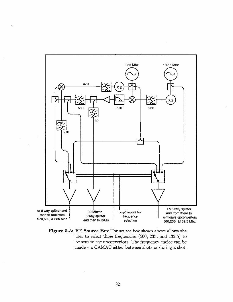
235 Mhz
470 r-.X 2
500 550
30
970
L
I17
to 8 way splitter andthen to receivers
970,500, & 235 Mhz
30 Mhz to6 way splitter
and then to I&Q's
i - .1
Logic inputs forfrequencyselection
To 8 way splitterand from there to
mmwave upconvertors500,235, &132.5 Mhz
Figure 5-3: RF Source Box The source box shown above allows theuser to select three frequencies (500, 235, and 132.5) tobe sent to the upconvertors. The frequency choice can bemade via CAMAC either between shots or during a shot.
82
132.5 Mhz
265
L414404

sidebands are suppressed by 20dB relative to the two transmitted sidebands. Two 18
dB isolators are needed to prevent pulling of the oscillator frequency by changes in
the power reflected by the plasma.
Experiments on JET [55] showed very rapid (~ lps) 30 dB changes in the signal
amplitude returned from the plasma. For the C-Mod reflectometer, the two returned
sidebands, which can each vary by 30 dB, needed to be mixed. To mix the two
returned sidebands without introducing large variations in the conversion loss, one
sideband is passed through a limiting ampb giving a constant 10 dBm output which
is put into the LO of a mixer. The other sideband, after being mixed with 970 MHz,
is then mixed with the limited signal producing a 30 MHz signal carrying the group
delay measurement. Since only one sideband has been limited, the power can still
vary greatly. Before making a final phase measurement, the signal is limited again,
then sent to the phase detectors. This system has a dynamic range of 50 dB with a
phase variation of less than five degrees.
The bandwidth of the input to the limiting amp should be equal to the bandwidth
of the filters on the output of the phase detectors in order for the quadrature sum
of the phase detector outputs to remain constant. For this reason, when profile
information was the primary interest, 2 KHz wide crystal filters centered about 30
MHz were placed before the 30 MHz limiting amp. This eliminated the possibility of
studying fluctuations on that particular channel. Typically, this filter was used in all
but the 88 GHz channel. Figure 5-4 shows the amplitude of the quadrature sum of
the two outputs with and without the crystal filter.
Three different upconversion frequencies can be generated for the transmitter and
receiver discussed above. When operating with the very narrow bandpass filters
described above, the difference frequency between doubled upconversion frequency
and the downconversion frequency must be good to a few hundred hertz. This nar-
row bandpass was not planned for when ordering the 970 and 500 MHz oscillators.
These oscillators could not be tuned enough to bring them within the filter band-
bA limiting amp is an amplifier designed to run in saturation. The output power (typically 10dBm) is independent of the input power. These amps serve the same purpose as automatic gaincontrol (AGC) amps. A limiting amp typically settles faster but is noisier than an AGC amp.
83
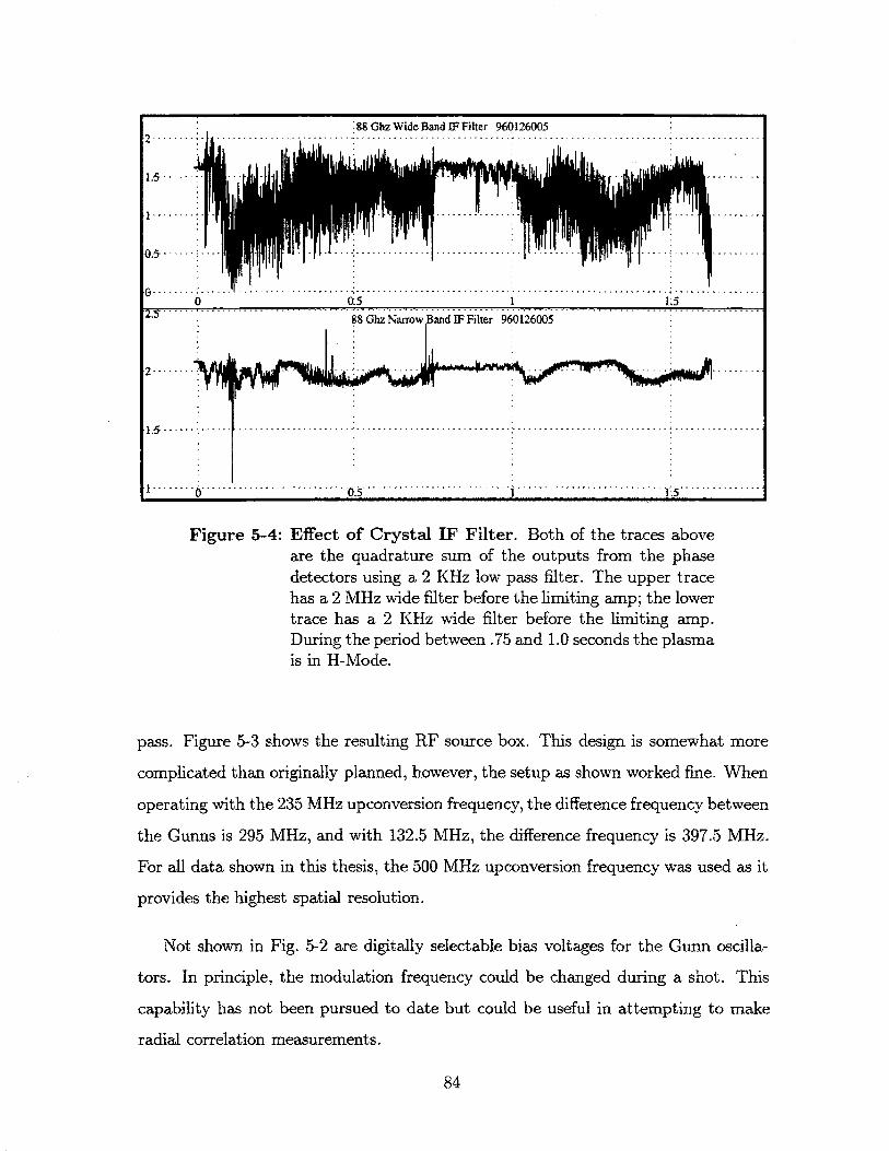
2 1h 1,88 Ghz Wide Band IF Filter 960126005
0 0.5 1:L58Ghz Narrow Band IF Filter 960126005
....... ....................................... 1
Figure 5-4: Effect of Crystal IF Filter. Both of the traces aboveare the quadrature sum of the outputs from the phasedetectors using a 2 KHz low pass filter. The upper tracehas a 2 MHz wide filter before the limiting amp; the lowertrace has a 2 KHz wide filter before the limiting amp.During the period between .75 and 1.0 seconds the plasmais in H-Mode.
pass. Figure 5-3 shows the resulting RF source box. This design is somewhat more
complicated than originally planned, however, the setup as shown worked fine. When
operating with the 235 MHz upconversion frequency, the difference frequency between
the Gunns is 295 MHz, and with 132.5 MHz, the difference frequency is 397.5 MHz.
For all data shown in this thesis, the 500 MHz upconversion frequency was used as it
provides the highest spatial resolution.
Not shown in Fig. 5-2 are digitally selectable bias voltages for the Gunn oscilla-
tors. In principle, the modulation frequency could be changed during a shot. This
capability has not been pursued to date but could be useful in attempting to make
radial correlation measurements.
84
............
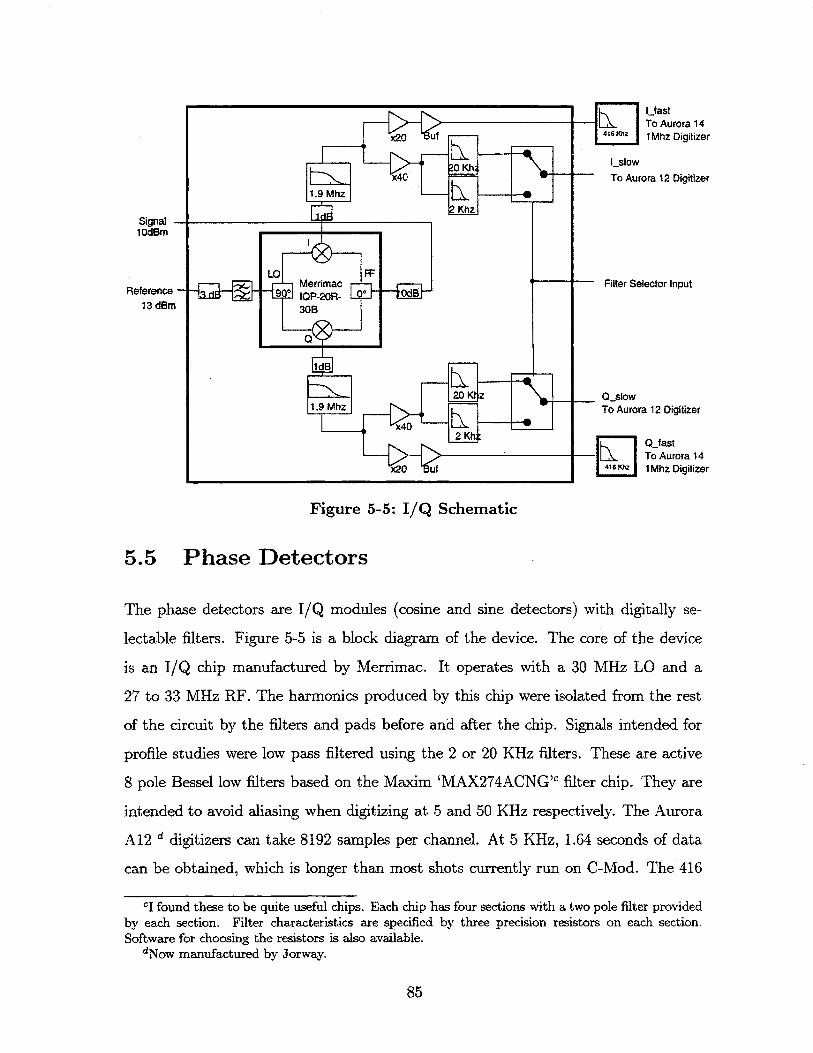
IfastTo Aurora 14
416 "Z 1Mhz Digitizer
I 2Slow
To Aurora 12 Digitizer
X20 uf -\ 1
0~ K
1.9L Mhz --2 Khz
LOFF
9O* Ip-2R 0 --B
30B
0
1.9 Mhz
x 2 Kh
x20 :u
Figure 5-5: I/Q Schematic
5.5 Phase Detectors
The phase detectors are I/Q modules (cosine and sine detectors) with digitally se-
lectable filters. Figure 5-5 is a block diagram of the device. The core of the device
is an I/Q chip manufactured by Merrimac. It operates with a 30 MHz LO and a
27 to 33 MHz RF. The harmonics produced by this chip were isolated from the rest
of the circuit by the filters and pads before and after the chip. Signals intended for
profile studies were low pass filtered using the 2 or 20 KHz filters. These are active
8 pole Bessel low filters based on the Maxim 'MAX274ACNG'C filter chip. They are
intended to avoid aliasing when digitizing at 5 and 50 KHz respectively. The Aurora
A12 d digitizers can take 8192 samples per channel. At 5 KHz, 1.64 seconds of data
can be obtained, which is longer than most shots currently run on C-Mod. The 416
'I found these to be quite useful chips. Each chip has four sections with a two pole filter providedby each section. Filter characteristics are specified by three precision resistors on each section.Software for choosing the resistors is also available.
dNow manufactured by Jorway.
85
Signal10dBm
Reference -13 dBm
4
Filter Selector Input
CLsIowTo Aurora 12 Digitizer
0_fastTo Aurora 14
4 16 K Mhz Digitizer
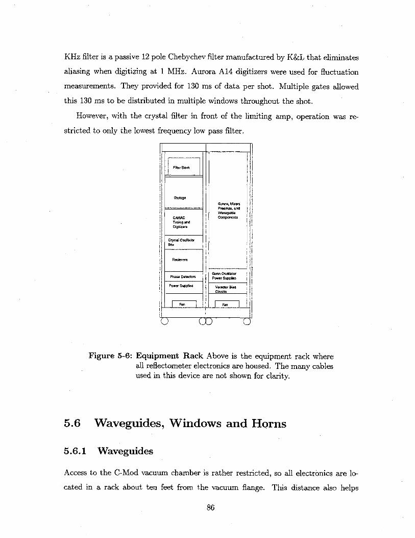
KHz filter is a passive 12 pole Chebychev filter manufactured by K&L that eliminates
aliasing when digitizing at 1 MHz. Aurora A14 digitizers were used for fluctuation
measurements. They provided for 130 ms of data per shot. Multiple gates allowed
this 130 ms to be distributed in multiple windows throughout the shot.
However, with the crystal filter in front of the limiting amp, operation was re-
stricted to only the lowest frequency low pass filter.
D CO
Figure 5-6: Equipment Rack Above is the equipment rack whereall reflectometer electronics are housed. The many cablesused in this device are not shown for clarity.
5.6 Waveguides, Windows and Horns
5.6.1 Waveguides
Access to the C-Mod vacuum chamber is rather restricted, so all electronics are lo-
cated in a rack about ten feet from the vacuum flange. This distance also helps
86
Plter Bank
Storage
CAMACTirning andDigitizers
Crystal OcItlorBOX
Redevers
Phase Deleclora
Power Spplies
Gun,,s, WixersPreamps. andWavepoidle
Cmoets
GVn Oscllator
Cirouits
7~7 7~Th

RefiectometerF Shieded
Equipment
Rac
ThomsonScatteingBeamline
Edge Thomson Thomsonin Igloo
Optics Assembly Optics Mounting
Rf Fast rScanning ProHousing-
&aa
WA 42 Overmoded Wavguides
Diagnostic support Stand
Li Li Li Li
Figure 5-7: A-Port Side View Also in this port, though not shown,are two cameras and several other spectroscopic diagnos-tics. Spectrometers for the Edge Thomson Scattering arelocated to the left of the reflectometer rack.
reduce the flux of X-rays and neutrons on microwave components.' This waveguide
run required tapering up to overmoded waveguide. WR-42 was used because it re-
duced the attenuation to an acceptable level and would not carry many modes other
than the desired TE10. In addition, WR-42 is the largest standard size waveguide
that can easily pass through a 1.33" "Conflat" vacuum window. A larger waveguide
would have greatly complicated the vacuum feedthroughs. With a very gradual bend
the waveguide could be oriented to match the angles of the horns without tapering
down again. For a continuous small perturbation to an overmoded waveguide, the
conversion to other modes is small unless the two modes are phase matched [56].
'Data on radiation damage to millimeter wave components is unavailable. There has been a
degradation over time of either sources or mixers. It is not clear if this is due to aging, operatorerror, or radiation damage.
87
A-port Covding
Vacu Vasse
Reflec ter
EdgThomson-ScafteringBeam Line
Cryostat Wall
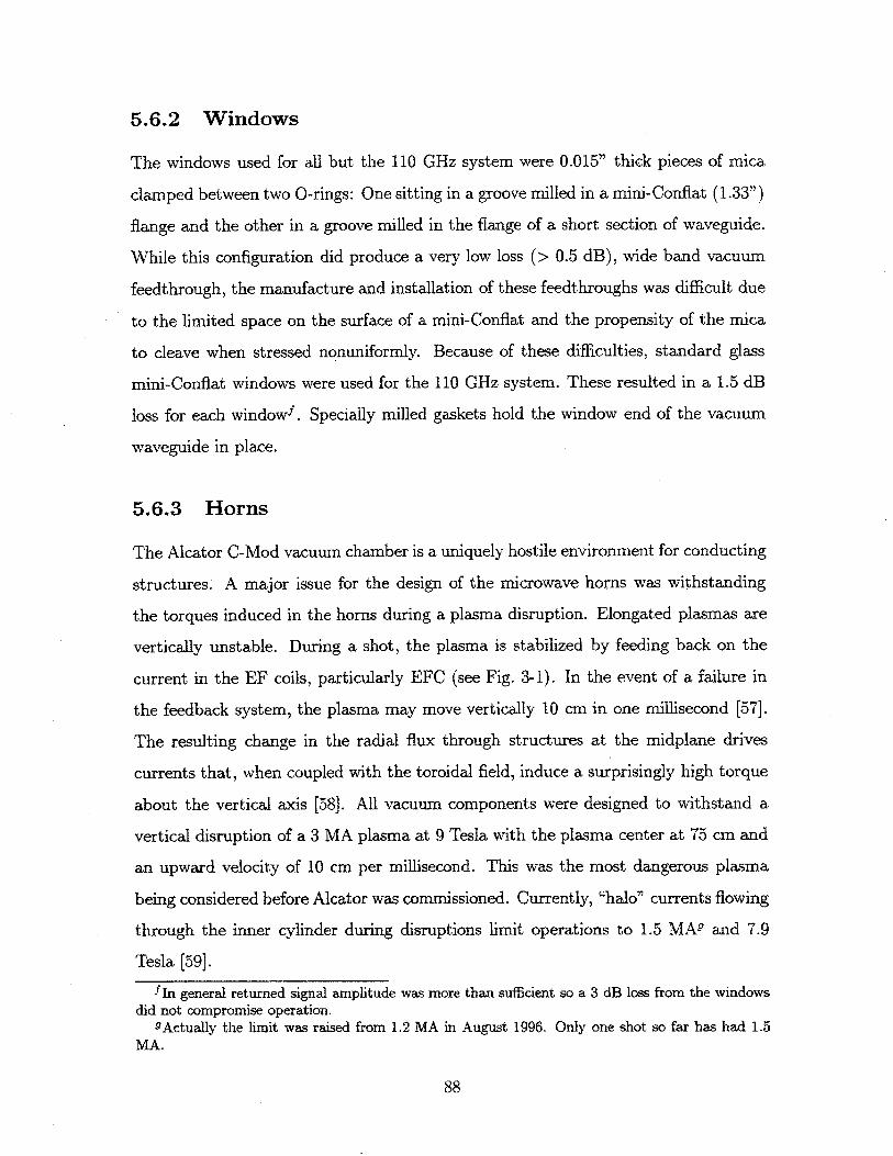
5.6.2 Windows
The windows used for all but the 110 GHz system were 0.015" thick pieces of mica
clamped between two 0-rings: One sitting in a groove milled in a mini-Conflat (1.33")
flange and the other in a groove milled in the flange of a short section of waveguide.
While this configuration did produce a very low loss (> 0.5 dB), wide band vacuum
feedthrough, the manufacture and installation of these feedthroughs was difficult due
to the limited space on the surface of a mini-Conflat and the propensity of the mica
to cleave when stressed nonuniformly. Because of these difficulties, standard glass
mini-Conflat windows were used for the 110 GHz system. These resulted in a 1.5 dB
loss for each windowf. Specially milled gaskets hold the window end of the vacuum
waveguide in place.
5.6.3 Horns
The Alcator C-Mod vacuum chamber is a uniquely hostile environment for conducting
structures. A major issue for the design of the microwave horns was withstanding
the torques induced in the horns during a plasma disruption. Elongated plasmas are
vertically unstable. During a shot, the plasma is stabilized by feeding back on the
current in the EF coils, particularly EFC (see Fig. 3-1). In the event of a failure in
the feedback system, the plasma may move vertically 10 cm in one millisecond [57].
The resulting change in the radial flux through structures at the midplane drives
currents that, when coupled with the toroidal field, induce a surprisingly high torque
about the vertical axis [58]. All vacuum components were designed to withstand a
vertical disruption of a 3 MA plasma at 9 Tesla with the plasma center at 75 cm and
an upward velocity of 10 cm per millisecond. This was the most dangerous plasma
being considered before Alcator was commissioned. Currently, "halo" currents flowing
through the inner cylinder during disruptions limit operations to 1.5 MA9 and 7.9
Tesla [59].
fIn general returned signal amplitude was more than sufficient so a 3 dB loss from the windowsdid not compromise operation.
9Actually the limit was raised from 1.2 MA in August 1996. Only one shot so far has had 1.5MA.
88

1.3850 and 60 Ghz
1.70
85.0*
4.00
75 and 88 Ghz
1.14
1.46
4.00
110 Ghz
0 0
+- 1.28
lf
Figure 5-8: Horn Antennas Above are shown cross sections of thehorn antennas mounted inside the C-Mod vacuum vessel.
89
4.82
95*
I
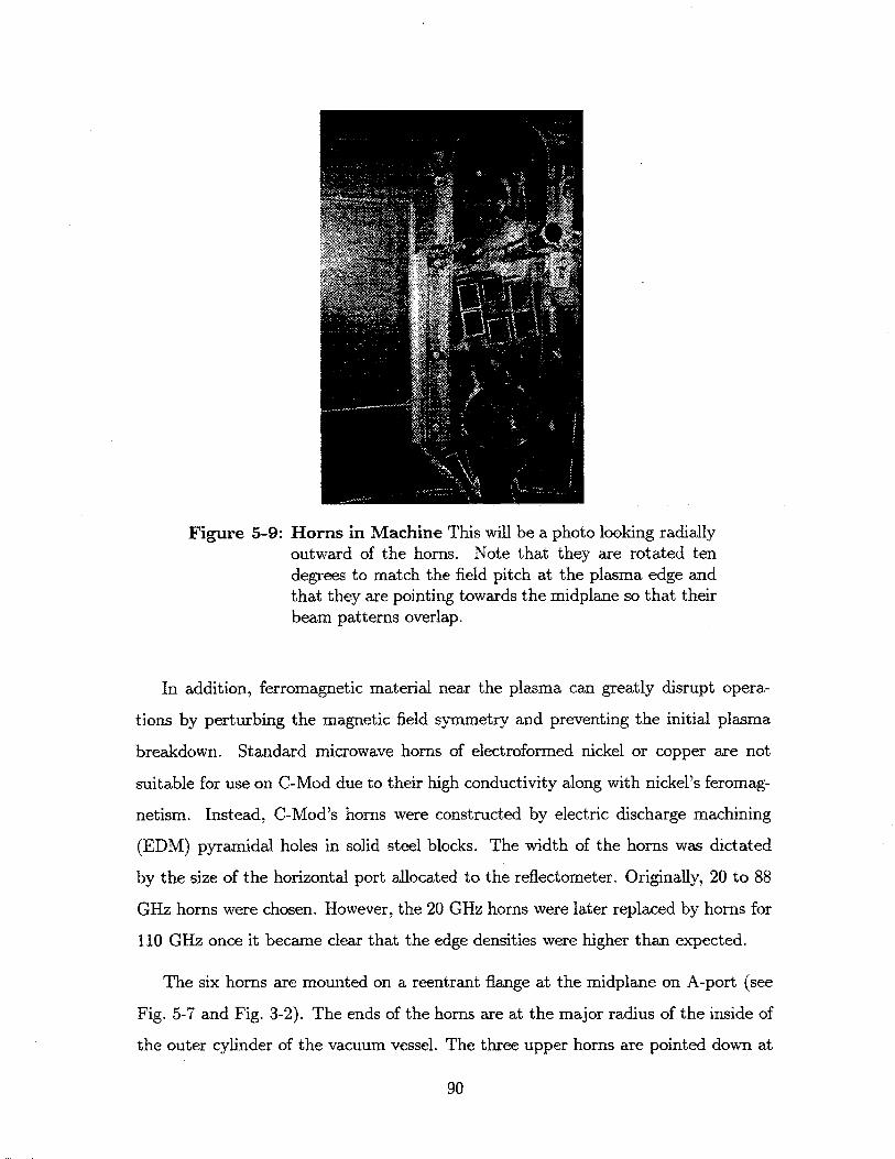
Figure 5-9: Horns in Machine This will be a photo looking radiallyoutward of the horns. Note that they are rotated tendegrees to match the field pitch at the plasma edge andthat they are pointing towards the midplane so that theirbeam patterns overlap.
In addition, ferromagnetic material near the plasma can greatly disrupt opera-
tions by perturbing the magnetic field symmetry and preventing the initial plasma
breakdown. Standard microwave horns of electroformed nickel or copper are not
suitable for use on C-Mod due to their high conductivity along with nickel's feromag-
netism. Instead, C-Mod's horns were constructed by electric discharge machining
(EDM) pyramidal holes in solid steel blocks. The width of the horns was dictated
by the size of the horizontal port allocated to the reflectometer. Originally, 20 to 88
GHz horns were chosen. However, the 20 GHz horns were later replaced by horns for
110 GHz once it became clear that the edge densities were higher than expected.
The six horns are mounted on a reentrant flange at the midplane on A-port (see
Fig. 5-7 and Fig. 3-2). The ends of the horns are at the major radius of the inside of
the outer cylinder of the vacuum vessel. The three upper horns are pointed down at
90

5 degrees and the lower horns are pointed up at 5 degrees so that their beam patterns
overlap at about 80 cm. The horns are rotated clockwise as seen by looking radially
in ten degreesh to match the expected field line pitch. The angle of the field at the
edge changes depending on the current, plasma shape, and toroidal field. Ten degrees
was chosen because the faraday shields of the ICRF antennas are set at this angle
so edge field pitch was expected to match this. (note: this was how I made that
choice. I should probably come up with some discussion of what this angle should
be in retrospect. It is not all together clear where the two modes separate with a
sheared field and a density gradient.)
5.7 Data Aquisition and Data Analysis
Scientists and students working on C-Mod have the luxury of using the MDS+ [60]
data aquisition system . This provides a very simple to use, menu-driven interface
between the CAMAC based data aquisition system and the user.
A 1 MHz clock is supplied to all diagnostics over an optical fiber. This clock
is then divided down in a "decoder" module to provide slower digitization rates.
Encoded in the clock is a start "event" four seconds before the anticipated initiation
of the plasma. MDS+ then calculates time bases for each signal. This central timing
system ensures that all digitizers use the same clock so that the timing of events seen
on different diagnostics can be reliably compared.
After a shot, data from all diagnostics are transferred over a fiber optic data
highway to a magnetic storage disk. Typically, within a few minutes of a shot, data
from all diagnostics are available to all users on the C-Mod cluster of workstations.
After a day's run, all data are archived in an optical disk "jukebox". All data from
all shots on C-Mod are available automatically in a few minutes. Shots that have
been accessed recently are stored on magnetic disk and are available within seconds.
Data are processed on Digital Alpha workstations using the IDL interpretive pro-
hBT and I, are always parallel.Replete with two computer scientists, Tom Fredian and Josh Stillerman, to whom the author is
greatly indebted
91
graming language. Processed data are stored on the same magnetic and optical disks
used for raw data.
92

Chapter 6
Profile Reconstruction
In this chapter, the steps involved in determining density profiles from the raw data
from the five reflectometer channels are described in detail. The resulting profiles
are compared with other diagnostics including the fast scanning probe, the grating
polychromator, Thomson scattering, and the two color interferometer. Along the
way, some of the common phenomena seen by the reflectometer will be presented. In
addition, the perturbation to the SOL by the fast scanning probe will be documented
and a couple of plausible models for this perturbation suggested.
6.1 Inversion Algorithm
In § 4.3.3, the location of the critical layer, Rc(fo), for a given frequency, fo, was
calculated from group delay measurements for an O-mode reflectometer via a simple
integration:
R.(fo) = a -d(f) df (445)Jo 27r2 df (f2f2)0 )
The integral above requires knowledge of d for all f between 0 and fo. For any
practical reflectometer, the number of data points is limited and some interpolation
scheme is needed. For a broad band swept system the number of data points is
dictated by sweep rate and signal to noise ratio. For a fixed frequency or narrow
93

band swept system, however, the number of data points is dictated by the number
of channels available. As a result, the number of data points measured in a profile is
much smaller. with a fixed frequency system. However, since no sweeping is required,
the time response can be much higher. On C-Mod, the term j is measured for up to
five different frequencies. Between measured frequencies, L is linearly interpolateddf eryitroae
with respect to f 2 ,. The density is assumed to be zero outside of the limiter radius
and linear between the limiter and the first data point. This will be discussed further
in § 6.3. The integral in Eq. 4.45 is approximated by the sum of 1 GHz wide bins:
Rc c to- d4l 2 1Rc(fo) =a - T-Z - x
Tr2 = [f2( l)]
c d4 "-~r fo -_+ x7 -f X. - acos A(6.1)2ir2 df (2fo ' 61
where f is in GHz. The third term on the right is required to deal with the singularity
in the integrand of Eq. 4.45 at f = fo. Figure 6-1 shows the evaluation of several
profiles using five data points as expected from the C-Mod Reflectometer and the
inversion routine described above. In general, the inversion agrees reasonably well
with the input profiles. Profiles with many sharp changes in slope, such as Fig. 5 in
Fig. 6-1, are not well represented due to the limited number of measurements.
6.2 Data Reduction
The steps involved in converting raw group delay measurements into density profiles
will be presented in the next few figures. Shot 9506090116 will be used as an example.
This shot was chosen because many of the phenomena typically measured by the re-
flectometer are present and the Thomson scattering system was absolutely calibrated
a few days after this run. This was a 7.9 tesla shot with a lithium pellet injected
anc oc f 2 , interpolating w.r.t. f biases the inversion toward concave profiles.'The shot numbering system deserves some explanation. The first two digits are the year, the
next two are the month, the next two are the day, and the last three are the shot on that day. Sothis was shot 11 on the ninth of June, 1995.
94

1.5
1.0
0.5
0.0-0.75 0.80 0.85 0.90 0.95
Radius (m)
3
1.0-
0.5
0.00.75 0.80 0.85 0.90 0.95
Radius (m)
5
1.5
1.0
0.5
0.00.75 0.80 0.85 0.90 0.95
Radius (M)
2
1.0
0.5
0.00.75 0.80 0.85 0.90 0.95
Radius (M)
4
1.0 -
0.5
0.00.75 0.80 0.85 0.90 0.95
Radius (n)
6
1.5
1.0-
0.5
0.00.75 0.80 0.85 0.90 0.95
Radius (m)
Model Profile Inversions. Input profiles are shownwith solid lines and the inversions are shown with dashedlines. The +'s mark the five densities where group delaysare measured.
95
Figure 6-1:
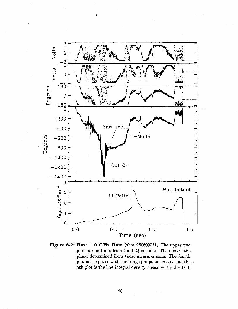
IA-
S~jj -
- --- A
- Saw Teet
- H-Mode
P.Cut On
Pol. Detach._Li Pellet
0.0 0.5Time (sec)
1.0 1.5
Figure 6-2: Raw 110 GHz Data (shot 950609011) The upper twoplots are outputs from the I/Q outputs. The next is thephase determined from these measurements. The fourthplot is the phase with the fringe jumps taken out, and the5th plot is the line integral density measured by the TCI.
96
0
2
0 1-
01-
U)U)5.4
U)
(U(U
;-4
0
-1800
-200
-400
-600
-800
-1000
-1200
-14004
3
0
0
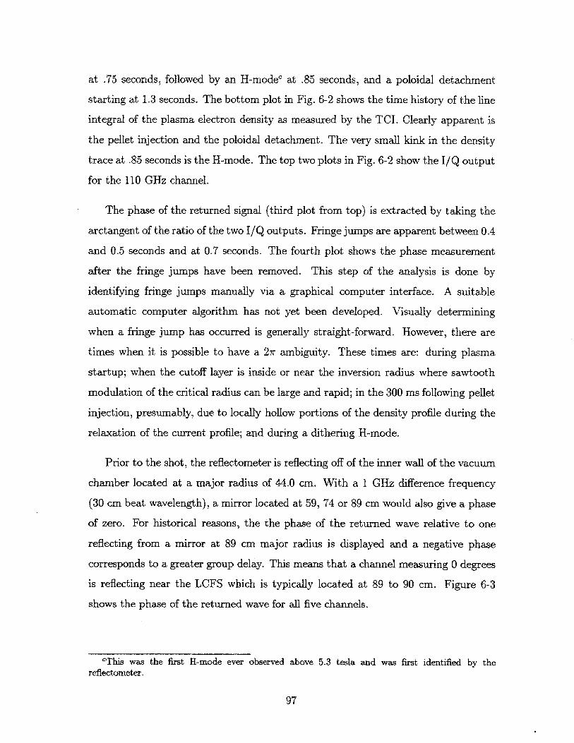
at .75 seconds, followed by an H-modec at .85 seconds, and a poloidal detachment
starting at 1.3 seconds. The bottom plot in Fig. 6-2 shows the time history of the line
integral of the plasma electron density as measured by the TCI. Clearly apparent is
the pellet injection and the poloidal detachment. The very small kink in the density
trace at .85 seconds is the H-mode. The top two plots in Fig. 6-2 show the I/Q output
for the 110 GHz channel.
The phase of the returned signal (third plot from top) is extracted by taking the
arctangent of the ratio of the two I/Q outputs. Fringe jumps are apparent between 0.4
and 0.5 seconds and at 0.7 seconds. The fourth plot shows the phase measurement
after the fringe jumps have been removed. This step of the analysis is done by
identifying fringe jumps manually via a graphical computer interface. A suitable
automatic computer algorithm has not yet been developed. Visually determining
when a fringe jump has occurred is generally straight-forward. However, there are
times when it is possible to have a 27r ambiguity. These times are: during plasma
startup; when the cutoff layer is inside or near the inversion radius where sawtooth
modulation of the critical radius can be large and rapid; in the 300 ms following pellet
injection, presumably, due to locally hollow portions of the density profile during the
relaxation of the current profile; and during a dithering H-mode.
Prior to the shot, the reflectometer is reflecting off of the inner wall of the vacuum
chamber located at a major radius of 44.0 cm. With a 1 GHz difference frequency
(30 cm beat wavelength), a mirror located at 59, 74 or 89 cm would also give a phase
of zero. For historical reasons, the the phase of the returned wave relative to one
reflecting from a mirror at 89 cm major radius is displayed and a negative phase
corresponds to a greater group delay. This means that a channel measuring 0 degrees
is reflecting near the LCFS which is typically located at 89 to 90 cm. Figure 6-3
shows the phase of the returned wave for all five channels.
cThis was the first H-mode ever observed above 5.3 tesla and was first identified by thereflectometer.
97
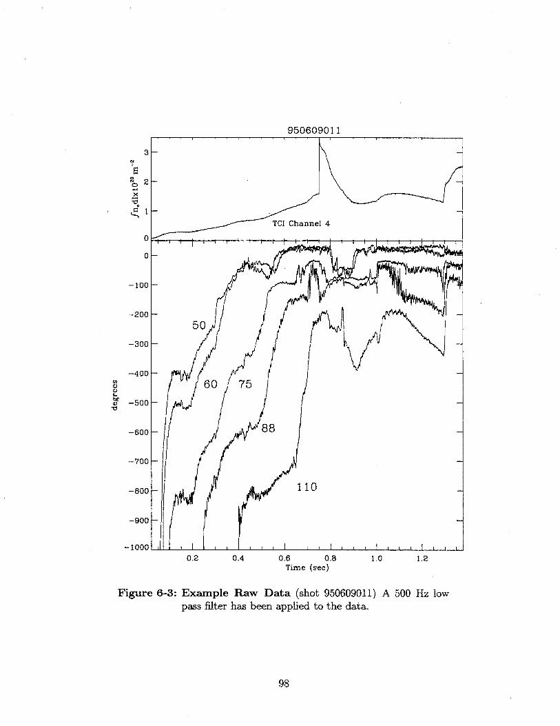
S0
x
950609011
3-
24
TCI Channel 4
0
0
-100-
-200-
-300-
-400 -
60 75
u -500-
-600- 88
-700-
-800 110
-900-
-10000.2 0.4 0.6 0.8 10 1.2
Time (sec)
Figure 6-3: Example Raw Data (shot 950609011) A 500 Hz lowpass filter has been applied to the data.
98
S.

6.3 Calibration
A key element of the operation of any reflectometer is absolute calibration. This has
been a challenge for several experiments [61, 24]. When launching into a metallic
vacuum chamber, reflections will not be limited to the inner wall, and power reflected
from objects other than the inner wall will corrupt the measured group delayd. In
principle, a swept frequency reflectometer can distinguish between reflections from
the inner wall and other structures in the machine. However, filtering in the receiver
must be carefully chosen to eliminate spurious reflections while maintaining sensitivity
to the expected range of profile shapes and locations [62]. For a fixed frequency
reflectometer, any spurious reflections can corrupt the returned signal. That this
is a problem for the C-Mod reflectometer can be seen in Fig. 6-4. This is from shot
950609013 which like 950609011 had a pellet and an H-mode. The H-mode between .8
and .86 seconds is much longer than the one in shot 11 and has a far more pronounced
effect on the 110 GHz channel. In fact, the phases measured for the 75, 88, and 110
GHz channels are inconsistent: they predict the critical layers for 75 and 88 GHz lie
further in the plasma than the critical layer for 110 GHz. By inferring an offset, these
channels can be brought into agreement. Justification for inferring this offset and a
protocol for doing so will occupy § 6.3.1 and § 6.3.2
6.3.1 High SOL Density Plasmas
Fig. 6-5 shows the phase measurements for shot 951206031. This was a particularly
high density, gas fueled, ohmic shot. Note that as the density rises, all channels of
the reflectometer go out to a fixed value. Also they reach this value in sequence,
from lowest to highest frequency. This value is independent of plasma shape and
position and remains the same from shot to shot. In particular it is independent
of gaps between the LCFS and any limiting surface. This effect can be seen on the
lower frequency channels for most diverted shots and on the higher frequency channels
dOther potential problems include amplitude to phase modulation in the receiver, pulling ofoscillators and induced phase shift in filters due to the magnetic fields induced by the EF coils, andpoor isolation between the receiving and launching arms of the receiver.
99
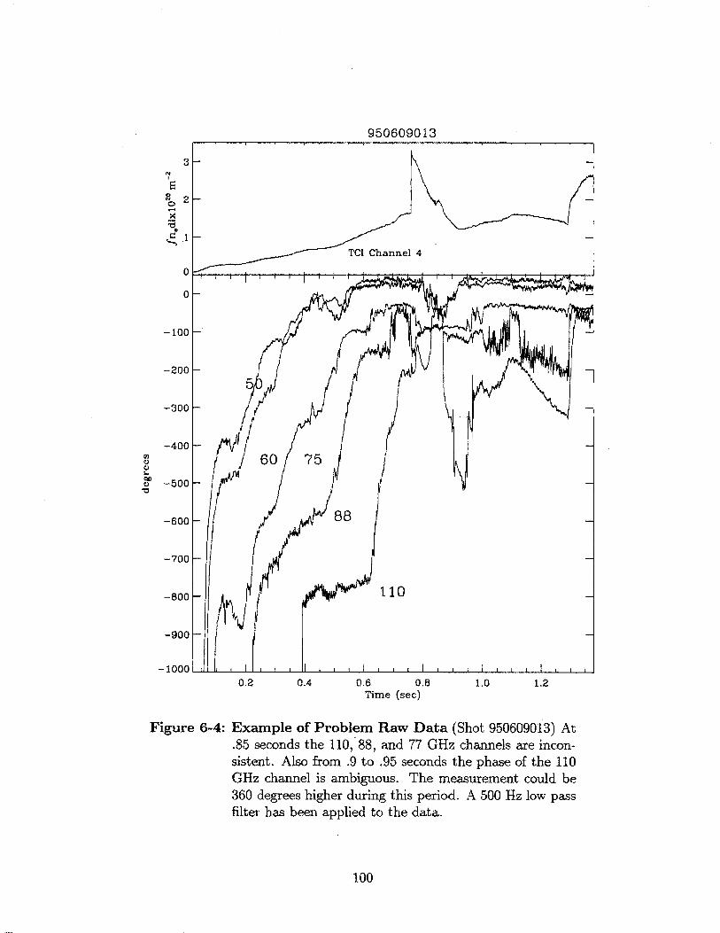
C
0.2 0-4 0.6 0.8Time (sec)
1.0 1.2
Example of Problem Raw Data (Shot 950609013) At.85 seconds the 110, 88, and 77 GHz channels are incon-sistent. Also from .9 to .95 seconds the phase of the 110GHz channel is ambiguous. The measurement could be360 degrees higher during this period. A 500 Hz low passfilter has been applied to the data.
100
3
2
0
950609013
Xv 4
60 75
- 110
C)
C)
C)
0
-100
-200
-300
-400
-500
-600
-700
-800
-900
-1000
Figure 6-4:

3 -
2-
1-
TCI Channel 4
0
0-
-100-
-200 50 Ghz
0
o 100
V -200
0
-100
-200
0
(D
-100
-200
IN
(3.1 x 101")
75 Ghz (6.9 x 101")
- 88 Ghz (9.6 x 10'9)-
110 Ghz (1.5 x 10²⁰)
0.2 0.4 0.6Time (sec)
Figure 6-5: High SOL Density Shot. Above is shown a particu-larly high SOL density shot. Note that from .9 to 1.0 sec-onds all four channels are at a fixed location near 0 = 0.This position is assumed to be the limiter radius.
101
EC
0
x
0.8 1.0
Horns
FSP\ Limiter
Vacuum Vessel (Mopped toHorn Location)
Figure 6-6: Fast Scanning Probe Mapping for a high field, highq shot.
on shots with extensive gas puffing, especially when the divertor is detached. This
effect is also visible, though less clearly, on shot 950609011 (see Fig. 6-3). Note that
channels 50 through 88 GHz all encounter an upper limit at .7, 1.05, and 1.3 seconds.
The only fixed object that can be causing this is the limiter located 16 cm toroidally
from the reflectometer horns (see Fig. 3-2). These observations point to there being
a steep gradient in the plasma density at the limiter radius, near the limiter. This
steep gradient can be used to calibrate the reflectometer by assuming a step function
in the plasma density at the limiter radius.
6.3.2 Comparison with Fast Scanning Probe
The fast scanning probe (FSP) is located 180 degrees toroidally from the reflectometer
(see § 3.2.3 and Fig. 3-2). In general, the FSP insertion into the SOL up to the LCFS
102

0.4
0.2
0
950607023
0
-0
-0
0.60 0.65 0.70 0.75 0.80 0.85 0.90 0.95
950607028
.4-
.2
.4 -
0.60 0.65 O.70 0.75 0.80 0.85 0.90 0.95
Figure 6-7: Closeup of Mapping of Fast Scanning Probe fortwo shots. These are expanded views of the flux mappingshown in Fig. 6-6. Shot 23 was a 3.5 tesla while shot 28was at 7.0 tesla. The mapping to the toroidal locationof the reflectometer is indicated by the stars. The starsin the lower portion indicate the FSP location on theopposite side of the machine.
103
0
0.0k
-0.21
-0.41

produces no significant change to the main plasma other than an occasional rise in
the radiation from molybdenum linese. For a small number of shots the edge q was
high enough1 for the location of the FSP to map along the field lines to the view of
the reflectometer (see Fig. 6-6). For ohmic plasmas with the proper field mapping, a
perturbation to the SOL caused by the FSP can be seen with the reflectometer. This
perturbation is not seen on shots where the flux tube intersected by the FSP does
not map to the reflectometer view. Figure 6-7 shows an expanded view in Fig. 6-6
of the mapping of the probe flux tube to the reflectometer toroidal position for two
shots. In shot 950607023, the mapping misses the reflectometer field of view and
no perturbation of the profile is observed. Shots 950607030, 28 and 29 (see Fig. 6-
8 & 6-9) are a density scan at constant BT and plasma current. In shot 30, only the
60 GHz channel was at the fixed position9 that is presumed to be the limiter radius
prior to the FSP insertion. The group delay is increased on the 60 GHz channel
during portions of the period of the probe insertion, but the other three channels
show no significant effect. Also note that the first perturbation on the 60 GHz profile
occurs at approximately the same time as the tip of the FSP crosses the limiter radius.
Profiles for the reflectometer during both the depleted phase and the post probe phase
are plotted with a smoothed profile from the FSP. Note the quite good agreement
during the depleted phase between the probe and the reflectometer. The reflectometer
profiles were obtained using the algorithm described earlier in this chapter with an
offset such that the fixed position attained by each reflectometer channel corresponds
to an step function in the density profile at the limiter radius.
Shots 950607028 and 29 show the same traits as shot 30 but at higher density. For
shot 28 only the 75 Ghz channel is affected and on shot 29 only the 88 Ghz channel
is significantly affected. The reflectometer profiles for each of these shots also show
better agreement with the FSP during the depleted phase. On shot 29 the limitations
of using only five fixed frequencies is apparent. The critical radius for the 110 GHz
channel probably does not change as the probe is inserted, however there are not
eThe probe head is constructed from molybdenum.f High Bt, low plasma current90n this day the 50 GHz channel was not operating.
104
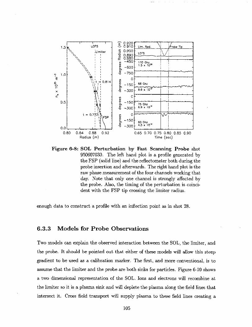
1.5 LCFS
Limiter
1.0
It = 0.814
0.5
t = 0.73t -FSP
I I
0.00.80 0.84 0.88 0.92
Radius (m)
a
0,9)9)ON9)-a
Id,9)9)ON9)*0
(.1,9)9)ON9)
~0
0,9)9)ON9)0
0.9200.9100.9000.8900.880-450
-600
-750
0
-150
-300
0
-150
-300
0
-150
-300
Lim.. Rod. \ r T
LCFS
110 Ghz1.5 x 10'0
88 Ghz
75 Ghz6.9 x 10l
60 Ghz4.5 x 10"
0.65 0.70 0.75 0.80 0.85 0.90Time (sec)
enough data to construct a profile with an inflection point as in shot 28.
6.3.3 Models for Probe Observations
Two models can explain the observed interaction between the SOL, the limiter, and
the probe. It should be pointed out that either of these models will allow this steep
gradient to be used as a calibration marker. The first, and more conventional, is to
assume that the limiter and the probe are both sinks for particles. Figure 6-10 shows
a two dimensional representation of the SOL. Ions and electrons will recombine at
the limiter so it is a plasma sink and will deplete the plasma along the field lines that
intersect it. Cross field transport will supply plasma to these field lines creating a
105
E
Cx
Figure 6-8: SOL Perturbation by Fast Scanning Probe shot950607030. The left hand plot is a profile generated bythe FSP (solid line) and the reflectometer both during theprobe insertion and afterwards. The right hand plot is theraw phase measurement of the four channels working thatday. Note that only one channel is strongly affected bythe probe. Also, the timing of the perturbation is coinci-dent with the FSP tip crossing the limiter radius.
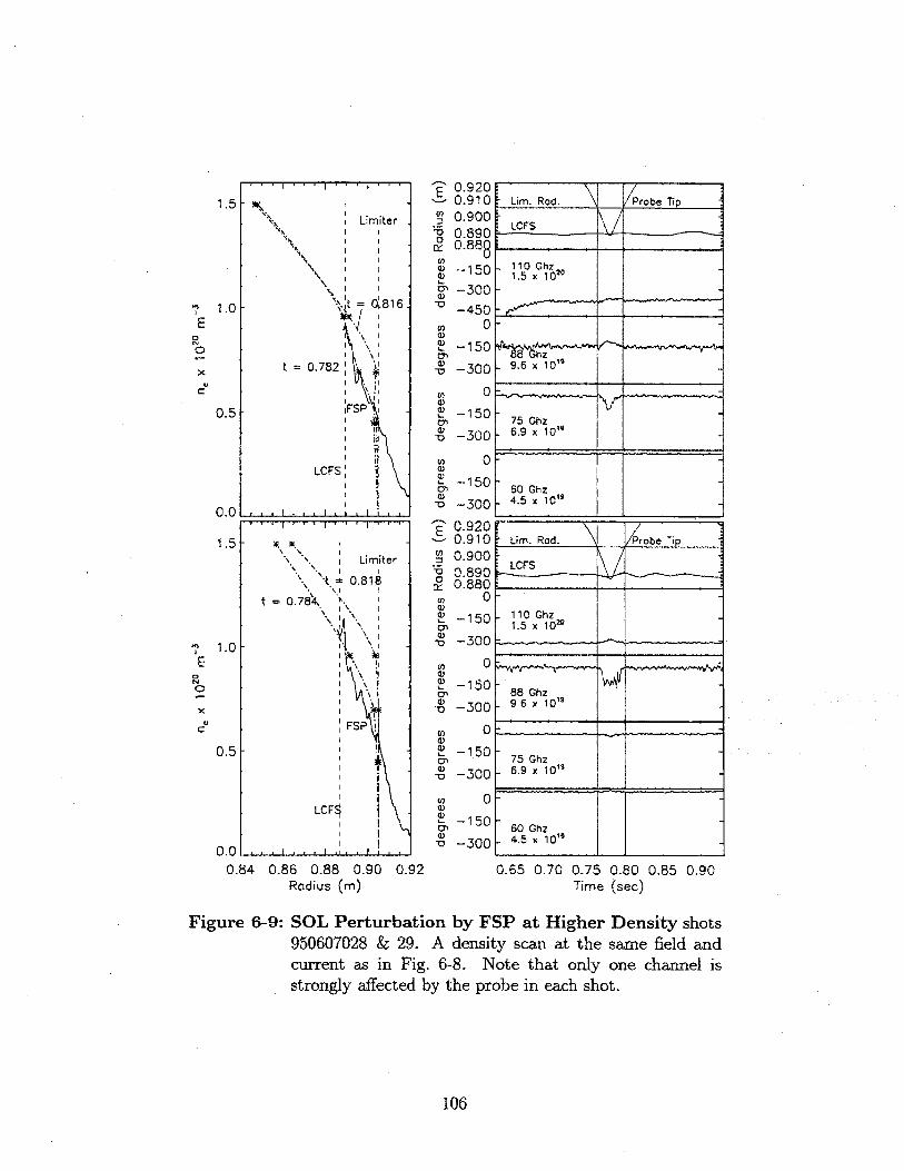
1.5
1.0E
C
0.5
0.0
1.5 - W-
Limiter
"t 0.818
t =0.7'4A.
1.0
FSP
0.5
LCF
0.0 .
0.84 0.86 0.88 0.90 0.92Radius (m)
0.9200.9100.9000.8900.888
-150
-300-450
0
-150
-300
Limiter
\ I
't 0,816.
t =0.782
F P
. LCFSI I
* Lc -s: -
cnci)ci)
0~Ici)-V
cc,ci)ci)
0'ci)
-V
0-150
-300
0
-150
-300
0.9200.9100.9000.8900.880
0
-150-300
0
-150
-3000
-150
-300
0
-150
-300
-Lim. Rod. \ Probe Tip
LCFS
.10 Ghz1.5 x 1020
9.6 x 10'
75 Ghz6.9 x 1Q0'
60 Ghz4.5 x 10'
Lim. Rod. \ Probe Tip
LCFS
110 Ghz1.5 x 1020
88 Ghz9,6 x 101
75 Ghz6.9 x 1ol"
-60 Ghz.4.5 x 101"
0.65 0.70 0.75 0.80 0.85 0.90Time (sec)
SOL Perturbation by FSP at Higher Density shots950607028 & 29. A density scan at the same field andcurrent as in Fig. 6-8. Note that only one channel isstrongly affected by the probe in each shot.
106
Cl,
-0
ci)
(D)
E
2x0
Figure 6-9:

net flow from the main plasma to the limiter. The reflectometer sits approximately
16 cm from the AB poloidal limiter. The fast scanning probe lies approximately 2.8
meters along the field line from the limiter. The divertor is approximately another
three meters further along the field line. If we take the probe to be located in a
region without significant flow Stangeby [63, 64] provides a rather simple model of
the density profile along the x axis. Assume a constant source, S, depositing particles
into the flux tube as shown. Defining the Mach number, M, and the ion sound speed,
C,:
V 'k(T + Te) 1/M = - where i= (6.2)
CSI
Stangeby derives the following relation from the momentum equation and continuity
dM S 1+ M 2
(6.3)dx nc, 1 - M 2 '
For S oc n this can be integrated to give:
L-x 2M n(M) 1= M and = M(6.4)L +M2 o + 2
where L is the distance from the probe to the limiter. The Bohm condition that
the velocity at the edge of the sheath equals the sound speed is assumed. From this
parameterization, the density variation along the flux tube is obtained. Note that the
reflectometer is expected to measure 60% of the value measured by the fast scanning
probe. This depletion in front of the reflectometer at the limiter radius may explain
the fixed value in the group delay measured by the reflectometer channels for high
SOL density shots.
The probe inserted into the SOL depletes the density along the flux tube that it
intersects. This increases the group delay for a channel previously seeing the limiter
radius and now looking deeper into the SOL and decreases the group delay for channels
looking deeper into the plasma. This can be seen in Fig. 6-9 for the 88 and 110 GHz
channels respectively. Stangeby [64] gives a value for the length of the flux tube
107

Main Plasma
LCFSS
>X
Limiter Reflectometer FSP
1.0-
0.8
0.6
c 0.4
0.20.0. . .
0.0 0.5 1.0 1.5 2.0 2.5 3.0Distance Along Flux Tube (m)
Figure 6-10: SOL Model
depleted by a probe of dimension d:
d2c~Le1 ~ d (6.5)
D.
The probe is 1.5 cm in diameter and for a 5 eV deuterium plasma c, ; 16 km/s giving
D± < 1.7m 2/s. This is far greater than the Bohm value of - 0.06m 2 /s or the value of
0.08 to 0.2 m2 /s estimated from fast scanning probe measurements [65]. So while this
calculation demonstrates that observing a perturbation of the SOL from the FSP is
expected, the upper limit it gives to the diffusion coefficient is so far removed from the
expected value that the measurement is not particularly useful beyond calibrating the
reflectometer. Matthews [66] has performed similar experiments on DITE using two
probes rather than a probe and a reflectometer. He was able to make quite detailed
measurements of Di by measuring the two dimensional profile of the perturbation
caused by one probe. Unfortunately the current C-Mod arrangement provides no
spacial resolution in the poloidal direction, preventing similar measurements from
being performed here.
108
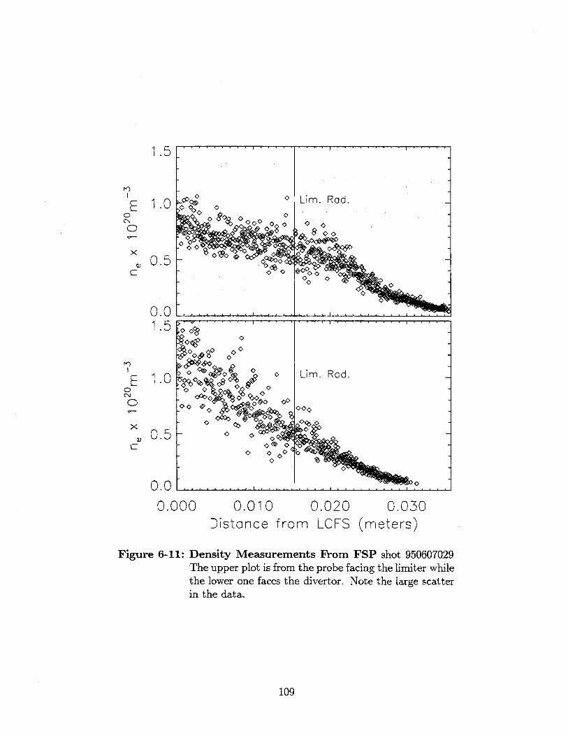
1.5
1.0
0.5
0.01.5
1.0
0.5
0.0
E 0* oo40o
0.000
Lim. Rod.
0 000 0 00
0
0.010 0.020 0.030Distance from LCFS (meters)
Figure 6-11: Density Measurements From FSP shot 950607029The upper plot is from the probe facing the limiter whilethe lower one faces the divertor. Note the large scatterin the data.
109
E0C
0
0CN0
x
C
0> 0
Lim. Rod.
Another model for the probe and limiter measurements assumes that the SOL
is extremely turbulent. For the comparisons shown in Fig. 6-9, the electron density
measured by the two working langmuir probes on the end of the FSP were smoothed
and averaged. Figure 6-11 shows the densities measured by the probe looking towards
the limiter and looking towards the divertor. The noise on the data is quite apparent
and presumably represents fluctuations in the plasma density. A density profile that
is varying greatly in space will bias a reflectometer measurement to larger major
radius as shown in Fig. 6-12. If the limiter somehow damps the oscillations in the
plasma, the reflectometer will see what appears to be a very steep gradient at the
limiter radius. If the probe moving into the SOL does the same thing, it will allow
a reflectometer channel that previously saw only to the limiter radius to see deeper
into the plasma, in agreement with what we observe.
6.4 Comparison with Other Diagnostics
6.4.1 Typical Features Observed with the Reflectometer
Returning to shot 950609011, the profile generated using the inversion scheme de-
scribed earlier is shown in Fig. 6-13. There are a few common phenomena that are
worth mentioning that are apparent during this shot. First, the deuterium pellet
that is fired into the plasma at .75 seconds has very little effect on the region of the
plasma that the reflectometer is observing. The pellet apparently deposits little in
the plasma edge, while the plasma inventory increases greatly (as shown by the TCI
in Fig. 6-2). Second, when strong gas puffing is applied, the region between the LCFS
and the limiter can reach densities of 1020 m- 3 or more. The gas valve is controlled
by the hybrid computer, which compares the density measured by the TCI with a
preprogrammed density waveform. Typically, the gas puff is turned off after a pellet
as the central density exceeds the preprogrammed density. The closing of the gas
valve results in a dramatic decrease in the SOL density and quite often an H-mode.
When the gas puff is turned back on again, the high SOL density returns. Third, a
110
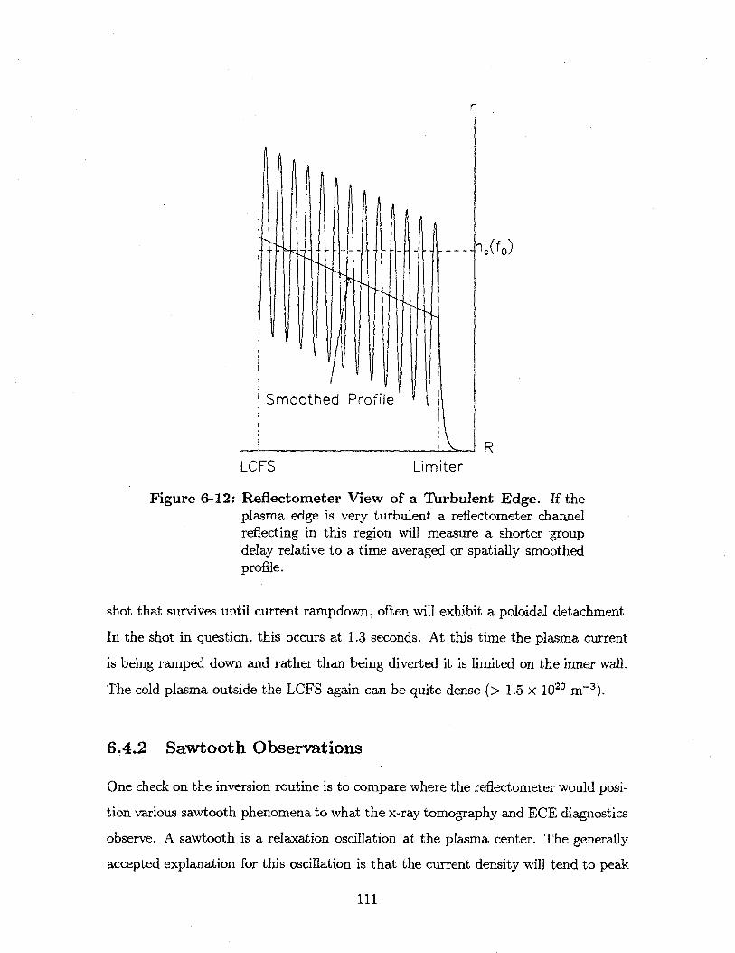
n
Smoothed Profile
RLCFS Limiter
Figure 6-12: Reflectometer View of a Turbulent Edge. If theplasma edge is very turbulent a reflectometer channelreflecting in this region will measure a shorter groupdelay relative to a time averaged or spatially smoothedprofile.
shot that survives until current rampdown, often will exhibit a poloidal detachment.
In the shot in question, this occurs at 1.3 seconds. At this time the plasma current
is being ramped down and rather than being diverted it is limited on the inner wall.
The cold plasma outside the LCFS again can be quite dense (> 1.5 x 10²⁰ m-3 ).
6.4.2 Sawtooth Observations
One check on the inversion routine is to compare where the reflectometer would posi-
tion various sawtooth phenomena to what the x-ray tomography and ECE diagnostics
observe. A sawtooth is a relaxation oscillation at the plasma center. The generally
accepted explanation for this oscillation is that the current density will tend to peak
111

0.85 LCFS
E
0.80
0.75 Sawtooth Mixing Radius
Saw Tooth Inversion Radius
0.70 /\ t Gas Valve Voltage (0-10 V)0.70 Pellet
0.4 0.6 0.8 1.0 1.2 1.4Time (sec)
Figure 6-13: Density Profile Evolution for Shot 950609011.Contour spacing is 1019 m- 3 from 1 to 15 xlO'9 .
on axis where the conductivity is the highest. However if the current density gets too
high the central plasma is unstable to resistive tearing modes. During the sawtooth
crash, plasma inside the inversion radius mixes with plasma just outside the inversion
radiush. The effect on the density profile is shown schematically in Fig. 6-14. The
effect on the temperature profile is similar except the heat pulse generally extends
diffusively out to the plasma edge. The inversion radius is pretty clearly observed
via either ECE or x-ray tomography. Here the value for the inversion radius is taken
from the x-ray diagnostics. The mixing radius is where the temperature and density
are promptly effected by the sawtooth crash. The mixing radius is not as clearly de-
fined as the figure suggests. After the sawtooth collapse, the profile gradually peaks
up again to the presawtooth shape. At larger radii the plasma sees a perturbation
appearing on a diffusive time scale.
'The inversion radius is widely believed to be at the q = 1 surface.
112

Pre SawtoothPost Sawtooth
nversion Radius
Mixing Radius
Minor Radius
Figure 6-14: Crude Sawtooth Model. The density and tempera-ture profiles change in less than a millisecond from thedashed profile to the solid profile. The thin lines showhow the profile may evolve back to the pre-sawtoothprofile during the 10's of milliseconds before the nextsawtooth.
Figure 6-15 shows sawtooth signals from the reflectometer and several of the GPC
channels. Channel 5 of the GPC shows a very rapid upward spike in the temperature
at the sawtooth crash. This channel is clearly looking in the region between the
inversion radius and the mixing radius. Channel 6 however has a more rounded
shape, putting it near or just inside the mixing radius. This places the mixing radius
somewhere between 0.75 and 0.78 meters major radius. Looking at the 110 GHz
reflectometer channel for this shot in the top plot in Fig. 6-15, three distinct sawtooth
responses can be seen as the plasma density is ramped up. Before 0.41 seconds the
group delay modulation from the sawteeth is too large for the reflectometer to follow.
Presumably, this corresponds to a presawtooth location for the critical layer inside
the inversion radius. From 0.41 to 0.52 seconds the reflectometer sees a very rapid
spike corresponding to a reduced group delay. Since the group delay is reduced, the
channel is looking outside the inversion radius. The very rapid response implies that
the critical layer is inside the mixing radius. The slower sawtooth response to the
113
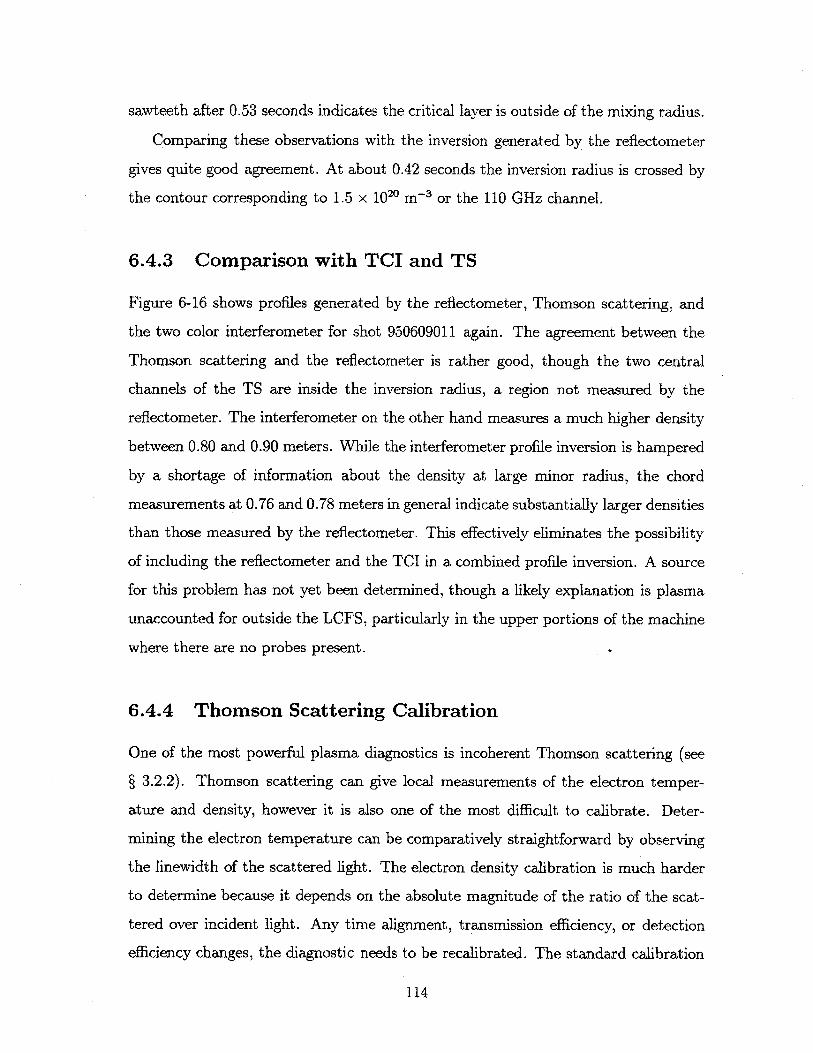
sawteeth after 0.53 seconds indicates the critical layer is outside of the mixing radius.
Comparing these observations with the inversion generated by the reflectometer
gives quite good agreement. At about 0.42 seconds the inversion radius is crossed by
the contour corresponding to 1.5 x 10²⁰ m- or the 110 GHz channel.
6.4.3 Comparison with TCI and TS
Figure 6-16 shows profiles generated by the reflectometer, Thomson scattering, and
the two color interferometer for shot 950609011 again. The agreement between the
Thomson scattering and the reflectometer is rather good, though the two central
channels of the TS are inside the inversion radius, a region not measured by the
reflectometer. The interferometer on the other hand measures a much higher density
between 0.80 and 0.90 meters. While the interferometer profile inversion is hampered
by a shortage of information about the density at large minor radius, the chord
measurements at 0.76 and 0.78 meters in general indicate substantially larger densities
than those measured by the reflectometer. This effectively eliminates the possibility
of including the reflectometer and the TCI in a combined profile inversion. A source
for this problem has not yet been determined, though a likely explanation is plasma
unaccounted for outside the LCFS, particularly in the upper portions of the machine
where there are no probes present.
6.4.4 Thomson Scattering Calibration
One of the most powerful plasma diagnostics is incoherent Thomson scattering (see
§ 3.2.2). Thomson scattering can give local measurements of the electron temper-
ature and density, however it is also one of the most difficult to calibrate. Deter-
mining the electron temperature can be comparatively straightforward by observing
the linewidth of the scattered light. The electron density calibration is much harder
to determine because it depends on the absolute magnitude of the ratio of the scat-
tered over incident light. Any time alignment, transmission efficiency, or detection
efficiency changes, the diagnostic needs to be recalibrated. The standard calibration
114
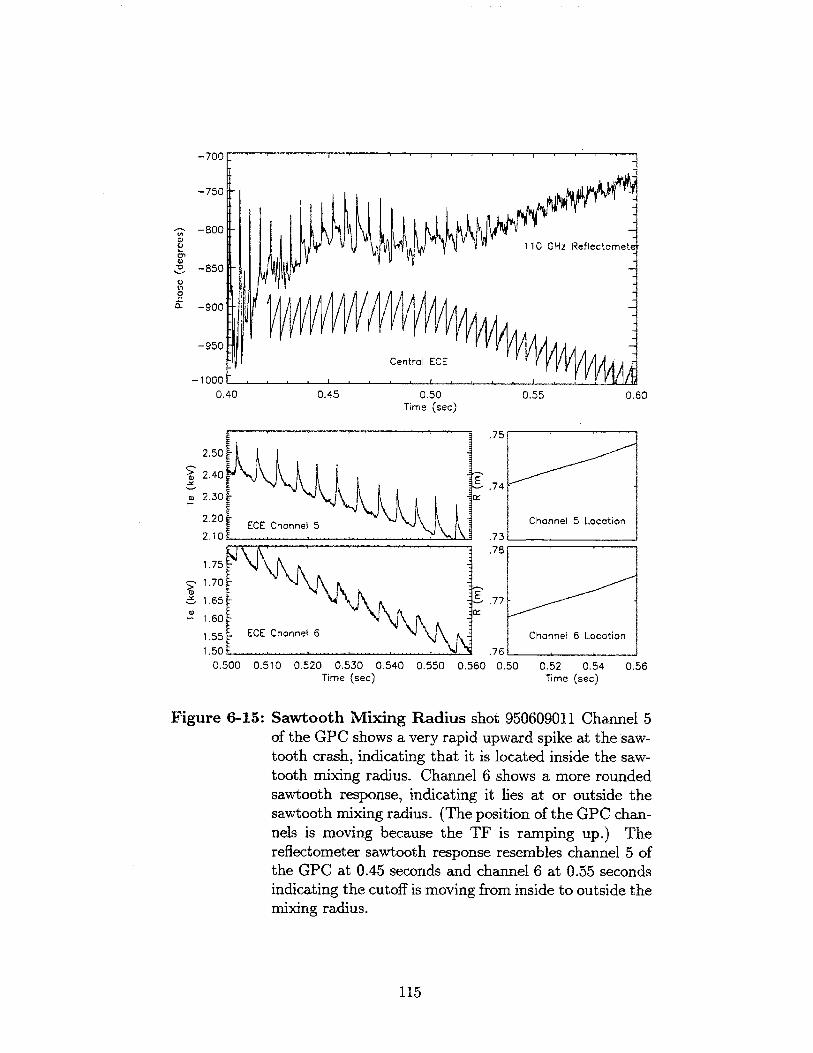
-70L
a-)
-750
-800
-850
-900
-950
-10000.40
2.'50
2.40
2.30
2.20
210
£1)
1. ..
1.75
1.70
.65
1.60
1.551.50
0.500
Figure 6-15:
0.45 0.50Time (Sec)
0.55 0.60
.75
.74
Channel 5 Location
.73
.78
.77
!ECEChannel 6 Channel 6 Location
76.0.510 0.520 0.530 0.540 0.550 0.560 0.50 0.52 0.54 0.56
Time (sec) Time (sec)
Sawtooth Mixing Radius shot 950609011 Channel 5of the GPC shows a very rapid upward spike at the saw-tooth crash, indicating that it is located inside the saw-tooth mixing radius. Channel 6 shows a more roundedsawtooth response, indicating it lies at or outside thesawtooth mixing radius. (The position of the GPC chan-nels is moving because the TF is ramping up.) Thereflectometer sawtooth response resembles channel 5 ofthe GPC at 0.45 seconds and channel 6 at 0.55 secondsindicating the cutoff is moving from inside to outside themixing radius.
115
110 GHz Ref lectomet
Central ECE-
ECE Channel 5
,, .
t = 0.50
0.70 0.75 0.80 0.85 0.90
t = 0.60
0.70 0.75 0.80 0.85Radius (m)
t = 0.70
0.90 0.70 0.75 0.80 0.85 0.90
Figure 6-16: Comparison of TCI, TS, and Reflectometer. shot950609011 The Thomson scattering diagnostic and thereflectometer agree reasonably well during the shot,however the interferometer gives a consistently highervalue at large R and a somewhat lower value in the cen-ter.
technique involves backfilling the vacuum chamber with some gas (typically hydro-
gen or argon) and observing light from Raman or Rayleigh scattering. Typically the
vacuum chamber must be kept at a uniform temperature and a whole day is needed
to get the desired statistics. On C-Mod this can only be accomplished during an
extended (one month or more) maintenance period. The TS can be cross calibrated
with the density profiles generated by the reflectometer or the interferometer or by
observing the cutoff on the ECE for particularly high density shots. This of course
transfers whatever systematic errors are present in one diagnostic to the Thomson
scattering.
An alternate, and potentially very accurate, technique for calibrating at least the
central channel of the TS is to observe the transition from transmitting to reflection
116
2.5
2.0 -
a
C
1.5
1 .0
0.5 0 TC
X ReflectometerA Thomson Scottering
i . - -
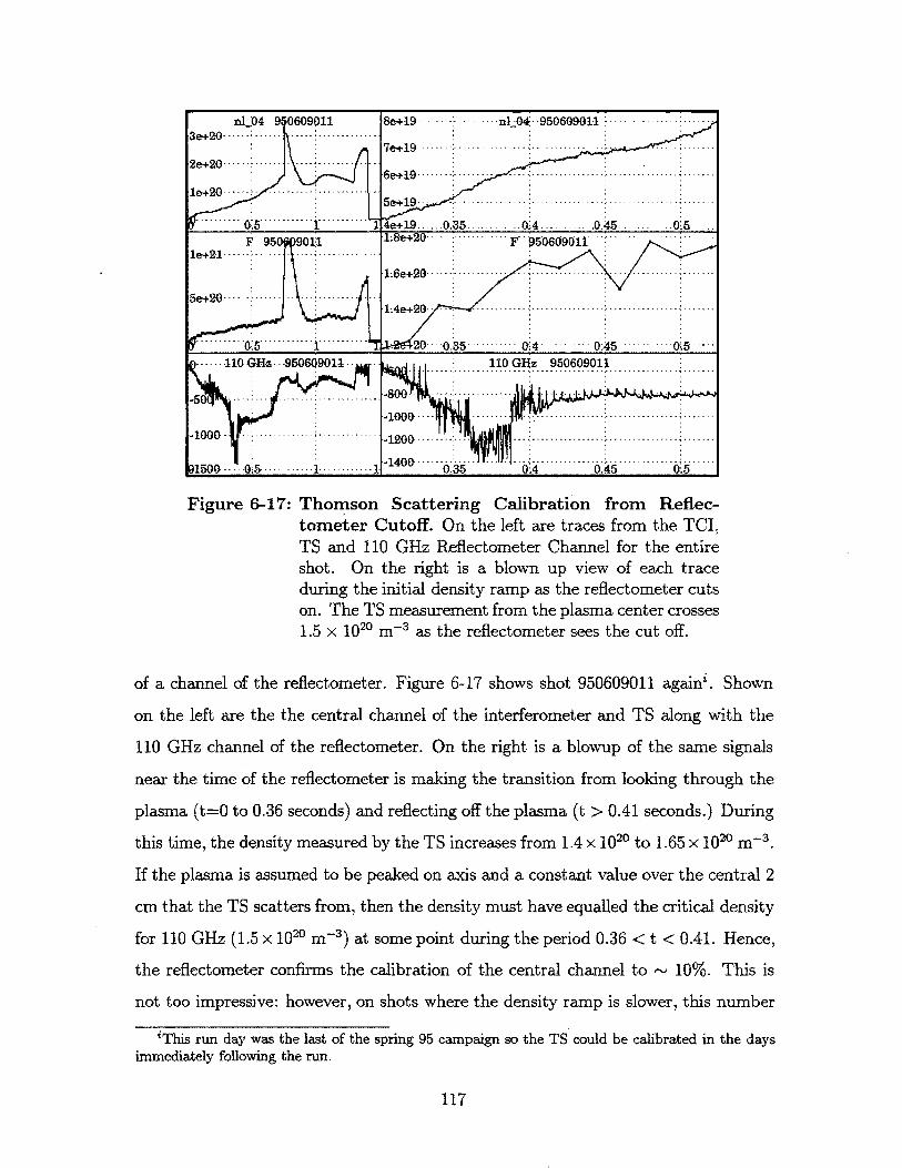
nI '04 9 06090113e+20 -...
2e+20 - -... .. .. -.. .. ...- .
1Ie+20 -...
---. . ..
F 950W901,1le+2 1 -. .. - ... - - .... - ..-.- ..-- .-- .
5e+20 --- - - -. -. -. -.. .. -.
.... ......
.... 110 GHZ -95060901.1 -
--5 .. .....
-4 000- - -- --- --
......... -0 - 1 '" U
Figure 6-17:
8e+19 nl_04 950609011 - -
7e+19 -.... .....
6 e+ 19 --.. .. - -... .- .. ...--..--..--. .-..--- ..--
5e+ 19 - - -.. . . -... . -.. ...... .. - -. ... .
+19- -0.35 . A 045 0 5..; .. + .. -..-- F .950609011
1.6 e+ 2 0 - - --. -.. -. -....-...-...-.
1:4e+20 -... .... .. .... . .
. 20 - -085 -.- 0 4 045 - 0 .5110 GHz 950609011
500 -..- - - -- - - ------.-- 5
120 --- --... . .. . -.. .. .. - -
.85 4 .. .... ....6 4 .. ....61i ...
Thomson Scattering Calibration from Reflec-tometer Cutoff. On the left are traces from the TCI,TS and 110 GHz Reflectometer Channel for the entireshot. On the right is a blown up view of each traceduring the initial density ramp as the reflectometer cutson. The TS measurement from the plasma center crosses1.5 x 1020 m-3 as the reflectometer sees the cut off.
of a channel of the reflectometer. Figure 6-17 shows shot 950609011 agains. Shown
on the left are the the central channel of the interferometer and TS along with the
110 GHz channel of the reflectometer. On the right is a blowup of the same signals
near the time of the reflectometer is making the transition from looking through the
plasma (t=0 to 0.36 seconds) and reflecting off the plasma (t > 0.41 seconds.) During
this time, the density measured by the TS increases from 1.4 x 10²⁰ to 1.65 x 10²⁰ m 3.
If the plasma is assumed to be peaked on axis and a constant value over the central 2
cm that the TS scatters from, then the density must have equalled the critical density
for 110 GHz (1.5 x 10²⁰ m-3) at some point during the period 0.36 < t < 0.41. Hence,
the reflectometer confirms the calibration of the central channel to - 10%. This is
not too impressive: however, on shots where the density ramp is slower, this number
This run day was the last of the spring 95 campaign so the TS could be calibrated in the daysimmediately following the run.
117
can be reduced to - 5%, making this calibration technique potentially more accurate
than traditional scattering calibrations. It should be pointed out that this technique
only assumes that the plasma density has a maximum on axis, the plasma density is
relatively flat near the center, and the definition of the plasma frequency is accurate,
all rather safe bets.
118

Chapter 7
Reflectometer Studies of H-modes
As was discussed in § 2.6 and § 3.3.4, an important topic in fusion research is un-
derstanding and controlling the characteristics of H-mode plasmas. The dominant
characteristic of these modes is the formation of a high gradient in density and tem-
perature at or near the LCFS. Reflectometry is particularly well suited to the study
of the evolution of this Steep Gradient Region (SGR). In this chapter, the transition
rate from an L-mode to an H-mode density profile and the width of the fluctuation
suppression region during C-Mod H-modes will be presented.
7.1 H-mode Characteristics
Figure 7-1 shows the raw data from a typical ICRF heated H-mode from the spring
of 1995. After 100 ms of application of 2 MW of ICRF power, the D, emission drops
dramatically at 0.82 seconds indicating a drop in particle recycling and a transition
from L to H mode. This is followed by a few ELMs and an ELM-free period to
0.85 seconds after which the ELMs start again and a return to L-mode at 0.885
seconds. During the ELM-free period the stored energy as measured by the magnetics
rises modestly from 90 to 115 kJ while the line integrated density rises much more
dramatically. However, showing the greatest change is the radiated power as measured
119
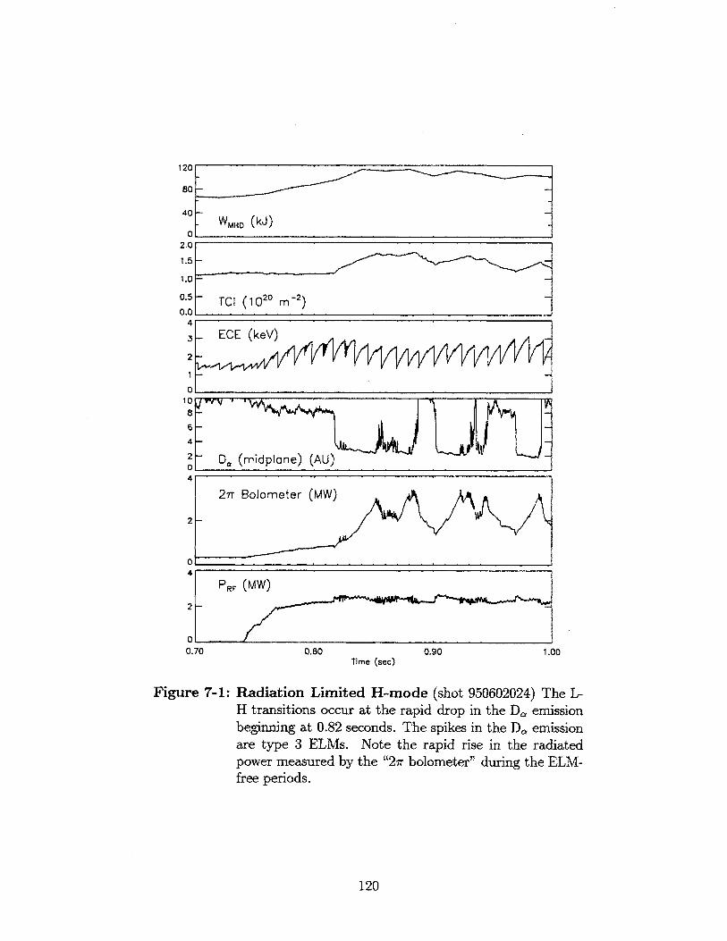
50-
4 WMHD(U
0.5- TOl (1020 m-2)0.0
4-
,3 ECE (keV)
2
01
D. (midplane) (AU)
21T Bolometer (MW)
2 -
4
PRF (MW)
0.70 0.80 Time (sec) 0.90 1.00
Figure 7-1: Radiation Limited H-mode (shot 950602024) The L-H transitions occur at the rapid drop in the D, emissionbeginning at 0.82 seconds. The spikes in the D, emissionare type 3 ELMs. Note the rapid rise in the radiatedpower measured by the "27r bolometer" during the ELM-free periods.
120

by the "27r bolometer"" indicating an accumulation of impurities. By the end of the
ELM-free period, the radiated power exceeds the applied RF power and approaches
the total input power (typically the ohmic power is 1 to 1.5 MW). This high radiated
power can not be sustained for long. ELMs starting at 0.85 reduce the radiated power,
presumably by pumping out impurities. This radiation limited behavior is typical of
operation during the spring '95 run period, with ELM-free periods during RF heating
lasting 20 ms or less. This is shorter than the energy confinement timeb. H-factors
(re/71TEs9-P) did not exceed 1.4 for any 5.3 tesla H-mode lasting on the order of an
energy confinement time.
7.1.1 Edge Temperature Threshold
There is a strong correlation between the temperature measured at the plasma edge
and the plasma state (L-mode, H-mode, or ELMy H-mode)c. Figure 7-2 shows the
outermost channel of the GPC positioned 2 cm inside the LCFS during the shot
discussed above. The sawtooth modulation of the edge temperature is evident. If a
sawtooth raises the edge temperature above 400 eV, the plasma enters an H-mode, and
below 320 eV the plasma returns to L-mode. Observing a GPC channel within a few
centimeters of the LCFS shows this pattern in general. However, the exact location
where the temperature needs to be a given value is still an area of research [67]. The
decline in the edge temperature during the H-mode is due to an increase in radiated
power (See Fig. 7-1). Note that the radiated power exceeds the input ICRF power
after 20 ms in H-mode, causing the edge to cool and drop below the threshold power.
121
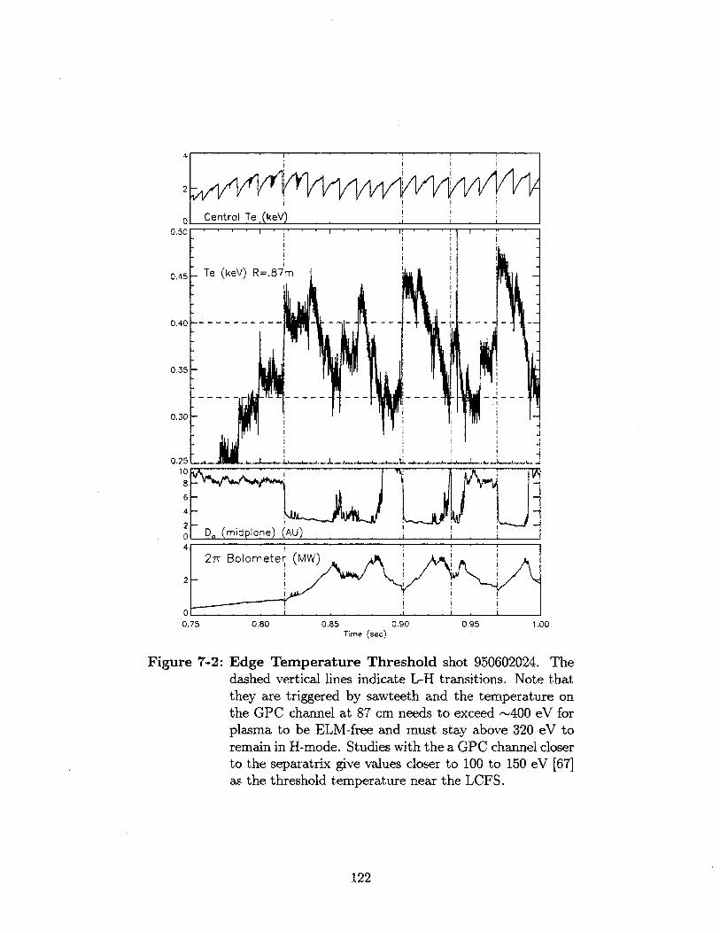
2
0 Central Te (keV0.50
0.45 Te (keV) R=.87m I
0.40 - - - - - - - - - - --- -- - ----
0.35 -
0.30 -
0.2510 ~i~
6 liiil-
2 - __ _ __ _ J _
0 , (jmidane)A )_ _ __ _ _ _ _
2
00.75 0.80 0.85
Time (sec)0.90 0.95 1.00
Figure 7-2: Edge Temperature Threshold shot 950602024. Thedashed vertical lines indicate L-H transitions. Note thatthey are triggered by sawteeth and the temperature onthe GPC channel at 87 cm needs to exceed -400 eV forplasma to be ELM-free and must stay above 320 eV toremain in H-mode. Studies with the a GPC channel closerto the separatrix give values closer to 100 to 150 eV [67]as the threshold temperature near the LCFS.
122
27T Boomete (MW)
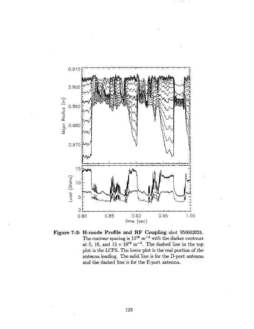
0,910
0.900
E0.890
0.880
0.870
C
0
15
10
5
00.80
Figure 7-3:
0.85 0.90time (sec)
0.95 1.00
H-mode Profile and RF Coupling shot 950602024.The contour spacing is 10"r m-3 with the darker contoursat 5, 10, and 15 x 10" m-. The dashed line in the topplot is the LCFS. The lower plot is the real portion of theantenna loading. The solid line is for the D-port antennaand the dashed line is for the E-port antenna.
123
7-

7.2 Electron Density Profile Evolution
Figure 7-3 shows the time evolution of the density profile during ICRF heating for
shot 950602024. Note that the density gradient at the LCFS increases dramatically
at the L-H transition. On the same time scale or slower, the density in the SOL
drops leading to a density gradientd on the order of 2 x 10²² m-4. The temperature
profile measured by the GPC during one percent BT scans also shows a steep gradient
located very close to the LCFS with a scale length on the order of 0.7 cm [68]. The
gradient during the ELMy period (ex. 0.865 seconds) is substantially less with the
greatest change being in the SOL density. At an H-L transition the SOL density
immediately increases while the profile inside the LCFS relaxes within 10 ms.
7.2.1 ICRF Loading
The loading to the ICRF antennas is strongly dependant on the SOL directly in
front of the antenna. The cutoff density for the fast ion cyclotron waves for the kl
spectra launched is - 7 x 10¹⁸ m- 3 (see § 3.3.2). This is well below the cutoff density
for the lowest frequency of the reflectometer (50 GHz, 3.1 x 10⁹ m-3 ). The flux
tube viewed by the reflectometer does not map directly to the region in front of the
antennas and the antenna Faraday shield sits one centimeter behind the A-B limiter.
Nonetheless, the loading should be expected to correlate somewhat with the lowest
densities measured by the reflectometer. The drop in antenna loading during H-mode
appears to correlate more with the formation of a steep gradient at the LCFS than
the density near the limiter radius. This indicates that the SOL in front of the ICRF
'The 27r bolometer is a diode sensitive to X-ray and UV emission from the plasma. It does notprovide as accurate a measurement of the emission as the bolometer arrays, however it has the fasttime response needed for studying these rapidly changing plasmas.
'For shot 950602024 -r- = WMHD/(POhmi, + PR1') ~ 120 kJ/4 MW = 30 ms'This section is included as edge temperature thresholds are key to understanding C-Mod H-
modes and the author contributed to its observation, though, of course the real credit belongs toHubbard and O'Shea (see references).
dThis value is at the limit of the reflectometer resolution, and the actual gradient may, in fact, begreater than this. This resolution is in part determined by observing the profiles calculated by thereflectometer during ELM free H-modes. On occasion, the group delay measurements will imply amultivalued density (see for example Fig. 7-10). The "overhang" is never greater than 0.5 cm, hencethe assumed error bar.
124

antennas is substantially different than the SOL in front of the reflectometer horns.
The sharp change in the density at the LCFS also contributes significantly to power
reflection, or the turbulence, which is higher when the gradient at the LCFS is lower,
increases transport to the region directly in front of the antenna (behind the poloidal
limiters and the antenna limiters).
The low loading values during ELM-free H-modes limit the power that can be
transmitted by the ICRH system. In addition, the sudden drops in loading at L-H
transitions trigger temporary transmitter shutdowns because they are indistinguish-
able from arcs in the ICRF transmission lines or antennas. To ameliorate the dele-
terious effects of the drop in antenna loading at the L-H transition, radial position
feedback on the ICRF loading was implemented beginning in November '95. The
outer gap (the gap between the LCFS and the limiter) is controlled by the hybrid-
computer (see page 42). Experimentally, the outer gap should be 1 to 2 cm to switch
from L to H-mode. After the H-mode commences, this can be reduced to as little
as 0.5 cm'. This motion is not enough to keep the loading at the L-mode level, but
it is sufficient to keep the ICRF from tripping out [70]. Because of this motion, the
density profile changes in the SOL are much less distinct after the implementation of
radial position feedback.
7.2.2 Profile Transition Time Scale
The density rise inside the LCFS can be extremely fast. The transition at 0.97 seconds
in Fig. 7-3 is an example of a fast transition with no ELMs. The density profile as
measured by the reflectometer changes from an L to an H-mode profile in less than
0.5 milliseconds. Two possible issues present themselves. First, is the density profile
monotonically decreasing as one travels from the plasma center to the edge? The 110
GHz channel may be reflecting off of a local maximum near the LCFS. Second, the
the 110 GHz channel reflecting off of the SGR rather than the actual cutoff further
'Based on correlations with the divertor probes, during L-mode, EFIT calculates the LCFScontour to within a few millimeters, however during H-mode the limitations of the EFIT currentmodel may increase this error to as much as a centimeter [69], so while the gap may be 0.5 cmaccording to EFIT, the actual gap may be closer to 1 cm.
125
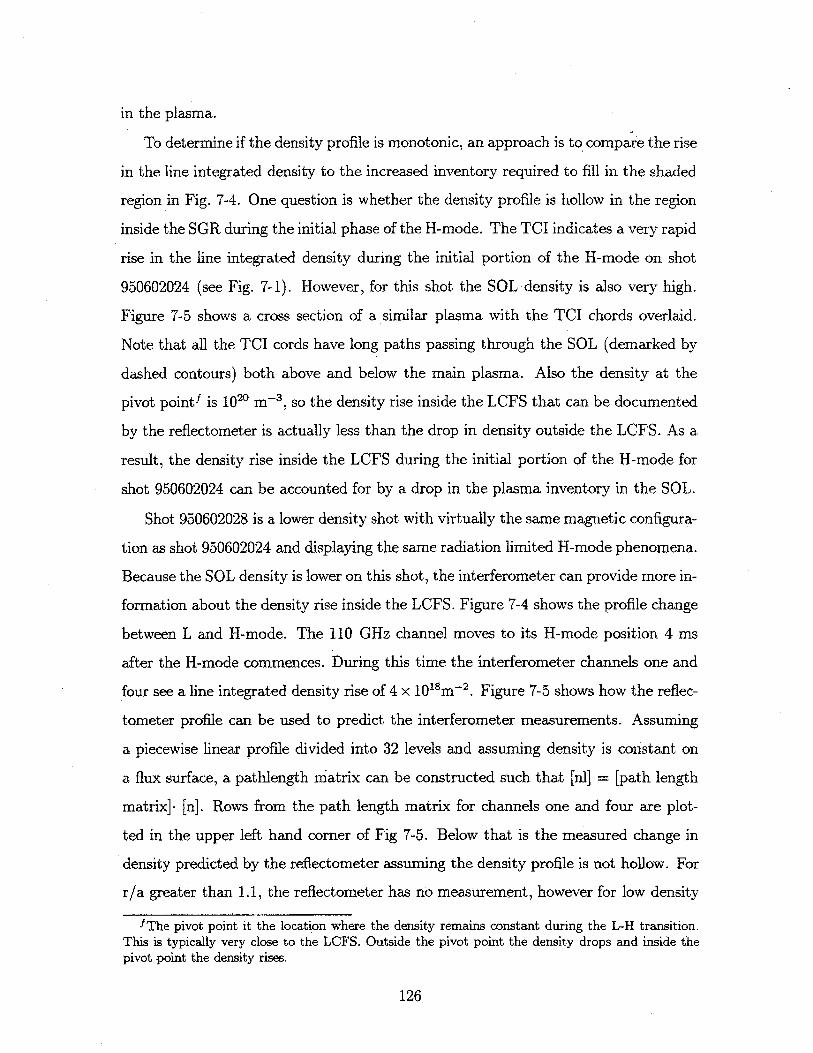
in the plasma.
To determine if the density profile is monotonic, an approach is to compare the rise
in the line integrated density to the increased inventory required to fill in the shaded
region in Fig. 7-4. One question is whether the density profile is hollow in the region
inside the SGR during the initial phase of the H-mode. The TCI indicates a very rapid
rise in the line integrated density during the initial portion of the H-mode on shot
950602024 (see Fig. 7-1). However, for this shot the SOL density is also very high.
Figure 7-5 shows a cross section of a similar plasma with the TCI chords overlaid.
Note that all the TCI cords have long paths passing through the SOL (demarked by
dashed contours) both above and below the main plasma. Also the density at the
pivot pointf is 1020 m-3 , so the density rise inside the LCFS that can be documented
by the reflectometer is actually less than the drop in density outside the LCFS. As a
result, the density rise inside the LCFS during the initial portion of the H-mode for
shot 950602024 can be accounted for by a drop in the plasma inventory in the SOL.
Shot 950602028 is a lower density shot with virtually the same magnetic configura-
tion as shot 950602024 and displaying the same radiation limited H-mode phenomena.
Because the SOL density is lower on this shot, the interferometer can provide more in-
formation about the density rise inside the LCFS. Figure 7-4 shows the profile change
between L and H-mode. The 110 GHz channel moves to its H-mode position 4 ms
after the H-mode commences. During this time the interferometer channels one and
four see a line integrated density rise of 4 x 10 8m-2 . Figure 7-5 shows how the reflec-
tometer profile can be used to predict the interferometer measurements. Assuming
a piecewise linear profile divided into 32 levels and assuming density is constant on
a flux surface, a pathlength matrix can be constructed such that [nl] = [path length
matrix]- [n]. Rows from the path length matrix for channels one and four are plot-
ted in the upper left hand corner of Fig 7-5. Below that is the measured change in
density predicted by the reflectometer assuming the density profile is not hollow. For
r/a greater than 1.1, the reflectometer has no measurement, however for low density
fThe pivot point it the location where the density remains constant during the L-H transition.This is typically very close to the LCFS. Outside the pivot point the density drops and inside thepivot point the density rises.
126
1.5-
1.0
0.5 - L-mode t = 0.8120
H- -H-mode t = 0.8165
0.0
0.70 0.80 0.90r/a
1.00 1.10
a,
I-
-om~0
0
0
1U5 Inner Wall B-dot coil0
-5-10
2.01.51.0 Min Plasma D.0.5r) (
0.400 350.30
S0.25 ~ GPC-9 (R=0.87 m)
O 0.98
A 0.96
c0.94 TCL_4
1.121.10
1.08 TCL_11.06
00 -200 Reflectometer 110 GHz
-400-600
0.812 0.813 0.814 0.815 0.816 0.817Time (seconds)
Figure 7-4: Rate of L-H Profile Change Shot 950602028 was acomparatively low density shot resulting in a rather slow(~ 4 ms) transition from an L-mode to an H-mode profile.The transition can be clearly seen on the inner wall mag-netics and the main plasma D, at 0.8129 seconds shortlyfollowing the arrival of a sawtooth heat pulse as seen bythe edge GPC at 0.8125 seconds. The 110 GHz reflec-tometer channel assumes an H-mode value after 0.8165seconds. The question is, is the shaded region filled in atthis time.
127
E0N0
0)

0.1
0.1
0.0
0.0
0.0
0.0
0.0.
0.
2
0 TCL1
6
4
2
06 -
4 .
2
0
2
40.0 0.5 1.0 1.5
1.....10
0.6
02
0.0
-0.2
-0.4-
-0.6
0.40 0.50 0.60 0.70 0.80 0.90 1.00 1.10R (m)
Figure 7-5: Modeling TCI Through L-H Transition shot950602028 On the right is the equilibrium reconstructionshowing the 32 contours of assumed constant density. Inthe upper left are the path length factors for each contourfor channels one and four of the TCI. Below that is thechange in density for each contour as measured by thereflectometer. At r/a greater than 1.1, the reflectometerhas no measurements hence the question mark.
128
E
0o
C
0.
0.
0.
-0.
-0.

shots such as 950602028, the density outside the LCFS is expected to be small. The
plot in the lower left corner shows the expected change in the line integrated density
compared to the measured change. Based on these measurements the shaded region
is not fully filled in at this time, 4 ms after the H-mode begins. This is however not
unexpected. The plasma source is either neutrals in the main chamber being ionized
in the plasma edge or plasma from the divertor and SOL being transported into the
main plasma via some anomalous pinch. The second source is at the edge with some
presumably narrow width dictated by edge transport issues. The neutrals entering
the plasma will also be ionized near the LCFS9. The time scale discussed here is short
relative to the 20 ms [71] particle confinement time for an L-mode plasma, so a local
maximum near the LCFS might be expected.
Unfortunately the errors on the above calculations are large. The three largest
sources of error are: the absolute calibration and inversion of the reflectometer (±2.5
mm in critical layer location), effective TCI chord location (±1 cm radially), and the
density outside the limiter radius. The upper plot in Fig. 7-6 shows the change in
density for a non monotonic profile (solid line). The dashed line is given by assuming
that the L-mode reflectometer measured profile is displaced inward relative to the
real profile and that the density outside the limiter radius is 0.15 x 10²⁰ m 3 ,or half
of the cutoff density for the lowest reflectometer frequency. During the H-mode the
density outside the limiter radius is assumed to go to zero. This will give a lower
bound on the change in the interferometer measurements required keep the H-mode
profile monotonic. This is the lower line plotted in the lower curve. The starred line
is the measured change in line integrated density and the upper curve is the measure-
ments expected with the measured reflectometer profile with the density outside the
limiter radius remaining constant during the L-H transition. Unfortunately, without
a point density measurement, the errors in the reflectometer and the interferometer
measurements due primarily to plasma outside the limiter radius.
gFor a 100 eV plasma the electron impact ionization and charge exchange reaction rates are 3and 3.75 x 10-cm3 /s respectively. Assuming an electron density of 1014 cm-3 and that the neutraldeuterium atoms have the Frank-Condon energy of 3 eV, the neutrals will travel 0.25 cm beforeeither ionizing or charge exchanging. Including multiple charge exchange events broadens the sourcesomewhat, but it is still limited to 1.5 cm from the plasma edge.
129

0.87? 0.6E
0A
o 0.2_-
0.0-0.2 ~- - ~-0.4-
0.0 0.5 1.0 1.5r/o
0.10 -
0.08
0.06-
0.04-
'0 0.02-
0.000 2 4 6 8 10
TCI Chord
Figure 7-6: Modeling TCI Through L-H Transition (part2).Please see text for explanation.
7.3 Fluctuation Suppression During H-mode
As was discussed in § 2.6, the anomalous transport of particles and energy in tokamak
plasmas is believed to be due to microinstabilities driven by gradients in constituent
temperature and/or density. The nature of these instabilities is poorly diagnosed
and hence poorly understood. During an H-mode, a transport barrier forms near the
LCFS. On other tokamaks, very high rotation velocities have been measured near
the LCFS, leading to the hypothesis that a radially sheared velocity profile near the
LCFS suppresses the microinstabilities or decorrelates them sufficiently to allow a
large pressure gradient to form. The reflectometer is an excellent qualitative tool for
studying this fluctuation suppression region or FSR because of its high sensitivity to
fluctuations and good radial spatial resolution.
130

Figure 7-7: Model of Scattering from a Rotating Mode. Thefigure on the left shows a Doppler wheel as used in aheterodyne interferometer. A mode rotating in a plasmacan give the same upsift in a reflectometer.
7.3.1 Note on Fluctuation Measurements
The study of plasma fluctuations via reflectometry is not straightforward and was not
intended to be the main focus of this thesis. Unlike collective Thomson scattering
or magnetic diagnostics, the frequency and amplitude of the returned phase does not
directly correlate with the motion of the plasma. The first issue is plasma rotation.
A good analogy is the Doppler wheel often used in heterodyne interferometry [38, 72]
(see Fig. 7-7). The upshifted frequency is:
1 + -sinOf' =f X C
wr- sin 0'
The angle and power of the upshifted beam is determined by the line spacing on
the wheel and the blaze of the grating. A plasma has perturbations that travel on
a flux surface in just such a fashion. A rotating metallic drum with some dents can
easily produce the Doppler wheel effect in a reflectometer mockup. (Without the
dents no Doppler shift is seen.) Nazikian [73] demonstrated this effect on TFTR.
Continuing the analogy, the blaze and the spacing of the waves in a tokamak plasma
are not givens, but the quantities one would hope to infer. Note that as a result
131

the frequency spectra seen by a reflectometer may not be the same as seen by other
diagnostics such as magnetics. A further complication is the sensitivity to a given
6n/n is higher as n approaches n,, so the slope of the profile near the cutoff can
greatly affect the sensitivity to fluctuations. This is particularly an issue for studying
fluctuation levels during L-H transitions when the gradients vary greatly.
In addition there are several problems unique to the C-Mod system. The intention
of the differential phase arrangement is to reduce the effects of fluctuations on the
group delay measurement. Fluctuations that appear coherently on both side bands
are largely subtracted out. The incoherent portions are not. This effectively amplifies
fading and power reflected from the edges of the beam pattern over the fluctuations
directly in front of the horn. In addition, the limiting amps that are required to
make reliable phase measurements of the beat wave, will produce harmonics of any
fluctuation signals. With these caveats, the reflectometer typically sees a rather
featureless fluctuation spectra with a slow decay out to the filter cutoff frequency of
416 kHz. The amplitude of the fluctuations does change dramatically depending on
the plasma state.
7.3.2 Rate of Fluctuation Suppression at L-H Transition
Figure 7-8 shows the suppression of fluctuations at an L-H transition. The diagnostic
that shows the transition first in low density plasmas is the magnetics on the inner wall
(second plot from the bottom). At 0.908625 seconds the fluctuations are suppressed.
On the reflectometer (third plot from the bottom), the transition is less clear, but
has certainly occurred by 0.90865 seconds. Also, the average phase of the returned
wave remains at the L-mode position for 50 ps after the fluctuation level has dropped.
This implies that the profile near the reflecting layer has not changed. So while some
of the observed drop in the fluctuations during an H-mode seen by the reflectometer
can be attributed to an increase in the gradient near the reflecting layer reducing the
reflectometer sensitivity to some Sn/n, the amplitude of the fluctuations also drops.
132

1.5
1.0 --- - -
EIC.
0.5-
0. ... .. ..
85 86 87 88 89 90Radius (cm) T
LCFS
0.500,40 Fluct. Power 100 to 400 kHz
0.300.20 -Integration Period0.10}--
3
21 --.- .
S -0 - -
-1 -
-2 .Raw Phase Data 88 GHz-3
50 dB/dt Inner WallU
0
N.0
0.9084 0.9086 0.9088 0.9090 0.9092Time (sec)
Figure 7-8: Fluctuation Suppression Viewed by ReflectometerChannel Initially in FSR. Shot 950602028. The 88GHz reflecting layer is within 0.6 cm of the LCFS priorto the H-mode and remains in the FSR. The transitioncan be seen on the magnetics at about 0.908625 seconds.The fluctuations on the reflectometer drop within 25ps ofthe transition.
133
H-mode t= 0.9090
L-mode t = 0.9085
7.3.3 Transport Barrier Width
The fluctuation level as observed by the reflectometer drops dramatically during most
H-modes. Figure 7-8 shows how the fluctuations drop quickly for a channel cut off
near the LCFS in the L-mode phase prior to the H-mode. However, the drop in
fluctuations is limited to a region near the LCFS. Figure 7-9 shows shot 950602024
again'. The main chamber and one channel from the divertor D, array are shown in
the top two plots. The divertor D, channel views the region near the inner nose of
the divertor. The D,, views elsewhere drop coincident with the L-H transition. Only
after the divertor D, emission and the SOL layer density drops does the fluctuation
level on the 75 GHz channel drop.
The FSR appears to be limited on the outside to 0.5 cm of the LCFS. The extent
of the FSR into the main plasma is more difficult to measure with reflectometry. For
virtually all ELM-free H-modes, all 5 channels of the reflectometer are reflected in
the SGR or at larger major radius within 500 ps of the transition. However for very
low initial density H-modes, the change in the electron density profile is slow enough
to allow for a brief study of the fluctuation level inside the main plasma after the H-
mode commences. Shot 950602019 was the lowest density shot to achieve ELM-free
H-modes on this day'. Figure 7-10 shows the first 1.5 ms of an H-mode during this
shot. At 0.8614 seconds, the fluctuation level measured by the magnetics on the inner
wall drops and is followed shortly by a drop in the D, emission (see lower two plots).
The phase signal measured with a 400 kHz bandwidth is shown in the middle trace.
Notice that the fluctuation level drops dramatically at 0.86205 seconds, 650 ps after
the start of the H-mode. The power in the band from 100 kHz to 400 kHz integrated
over 128 ps is displayed above the raw phase data. For at least the initial 300 ps of
the H-mode, the fluctuation level does not change significantly and the average phase
stays constant. The fluctuation level increases at 0.8618 seconds as the cutoff moves
hIt should be pointed out that this shot has a rather high lower triangularity (same shape asshown in Fig. 7-5) and a slot divertor, however the fluctuation phenomena are not unique to thismagnetic configuration.
At lower densities Z-effective is higher, so more power is radiated. This shot stays in H-modefor only 5 ms before returning to L-mode due to radiative energy losses.
134

6
4- MinD
20
1 .0
S0. 5
0.0 Divertor D.
0.80
Fluct at 100 kHz on 75 GHz
Fluct at 100 kHz on 88 GHz
0.82 0.84
Figure 7-9: Outer Limit of Fluctuation Suppression RegionDuring H-mode. Shot 950602024. The H-mode canbe seen to start at 0.817 seconds, however the fluctua-tions on the 75 GHz channel begin to drop only after the75 GHz cutoff layer moves into the SGR and the divertorD, begins to drop at 0.83 seconds.
135
0.905
0.900
0.895
0.890
0
a0
Reflectometer Profile0.885
0.
0.6
S0.4
0.2
0M1'0
0.8
0.6<0.4
0.2r)
0.86Time (sec)
0.88 0.90 0.92

84 86 88 90Radius (m)
LCFS
0.8 Fluct. Power 100 to
0.6<0,4
0.2 Integration Period
400 kHz I0 1
-2 - Row Phase Data 88 GHz
10 dB/dt Inner Wall
(n 0
1
Main Chomber Da
0.3
A
0.00.8615 0.8620
Time (sec)0.8625
Figure 7-10: Inner Limit of Radial Extent of Fluctuation Sup-pression Region Shot 950602019. The H-mode startsat 0.8614 seconds as witnessed by the magnetics. Thefluctuations observed by the reflectometer remain con-stant until 0.86175 seconds, indicating that the FSRdoes not extend 1.5 cm inside the LCFS during the ini-tial 300 ps of the H-mode.
136
.0
C
0.0
H-mode t = 0.8625L-mode t 0.8610
- - -. -0.5

from the L-mode to the H-mode position. This is to be expected as the profile near
the cutoff is flatter or nonmonotonic during this period
The profiles both before and after the L-H transition are shown in the top figure.
The 88 GHz cutoff density is shown with the horizontal dashed line. The cutoff
location moves from 0.874 to 0.892 meters between 0.8618 and 0.8621 seconds. For
at least the first 300 ps the FSR extends less than 1.8 cm inside the LCFS.
With an 0-mode reflectometer, this approach of measuring the FSR width is
very limited. A channel cutoff inside the plasma before the L-H transition gener-
ally changes to being cutoff in the SGR some time after the L-H transition with a
discontinuous jump. With the planned divertor cryo-pump, the density rise during
ELM-free H-modes may be controlled sufficiently to keep the density in the SGR be-
low the critical density of the highest reflectometer channel. An X-mode reflectometer
using the RHC on a machine where w,/wc < 1 would have more success with this
measurement as the location of the cutoff is not as dependent on the density profile.
7.4 Enhanced D, H-modes
7.4.1 Post-Boronization
In January of 1996, the machine walls were "boronized" [74, 75] (coated with boron
via plasma deposition). This greatly reduced the rate of high Z impurity accumulation
in H-mode plasmas and allowed H-factors of 2.5 to be reached in ELM-free plasmas.
Figure 7-11 shows a "trophy" shot from an impurity confinement study during this
period. The rise in the radiated power beginning at 0.7 seconds is due to an intentional
impurity injection (scandium). This shot demonstrates a very long confinement time
for impurities in ELM-free plasmas ~ 1 second [76]. After 0.86 seconds the D" light
iThe H-mode profile between the 88 and 110 GHz cutoffs is shown as a dashed line becauseduring this transient phase, there may be far more structure in the profile than the reflectometercan resolve. The group delay for the 110 GHz channel actually increases during the H-mode. Howeveron the 1 ms time scale, the profile at 0.83 meters (r/a = 0.7) probably does not change. The profilereconstruction routine, however, does not take this into account. The actual profile is expected tobe somewhat higher than shown in the few cm inside the LCFS and closer to the L-mode level near0.84 meters.
137

W5 - MHD (
50-
2 TC1 (10 20 m
4 ECE (keV) I
2 --
S- Da (midplane) (AU)6 --
4 -
2 -
4 - 27T Bolometer (MW)
2-
0
4
PRF (MW)
2--
0.50 0.60 0.70 0.80Time (sec)
0.90 1.00 1.10
Figure 7-11: ELM-free and EDA H-mode. shot 960214030 Theplasma is in an ELM-free H-mode from 0.6 to 0.86 sec-onds. At 0.7 seconds, scandium is injected which accel-erates the rise in impurity radiation. After 0.86 secondsthe plasma enters an Enhanced D, phase. Impurity con-finement is greatly reduced as witnessed by the drop inradiated power as seen by the 27r bolometer decays away.Also the TCI shows that the plasma inventory stabilizes.
138
1

rises and the radiation measured by the bolometer decays. Impurity confinement
drops to - 0.1 second [76] and the stored energy increases modestly. Very occasional
isolated ELMs have been observed during the period of elevated D, emission, but
none that have the periodicity of type three ELMs often seen during ohmic H-modes,
nor do they have a significant effect on the stored energy that one would expect from
type 1 ELMs. One possibility is that the emission we see is due to "grassy" ELMsk
that are too fast for the C-Mod diagnostics to observe or the response time of the
C-Mod SOL is long compared to the ELM period. Magnetic fluctuations are often
seen during these Enhanced D, (EDA)' H-modes [77] at typically 65 kHz, however
they saturate in amplitude rather than showing the exponential growth characteristic
of ELM precursors.
Since boronizing the machine walls, such EDA H-modes have become quite com-
mon. They present a very promising mode of operation for future fusion reactors as
their energy confinement time is quite high (H-factor - 2) yet the particle confine-
ment is greatly reduced from that of an ELM-free H-mode (see § 2.6.3). These are
effectively steady state H-modes with their duration dictated by operational issues,
in contrast to the H-modes from the spring '95 run whose duration were limited by
high radiated power due to impurity accumulation.
The reflectometer was handicapped during this run period due to two problems.
The first was a failure of a mixer in the 110 GHz system. The second was a change in
the interaction between the SOL and the limiter radius. In general, the steep gradient
previously seen at the limiter radius was not observed after boronization, except
during strong impurity puffing. The assumption is that the higher edge temperatures
seen after boronizing resulted in a narrower SOL. As a result the calibration technique
presented in § 6.3 was in general not available. However, shot 960214030 provides
a an opportunity to compare uncallibrated data from an ELM free H-mode and an
kGrassy ELMs have been observed to have many of the same qualities as the EDA H-modes inthat they reduce particle confinement without reducing the energy confinement greatly.
'The name for this type of plasma has changed with each conference in the last year. Theyhave also been called as Enhanced Recycling H-modes or High Recycling H-modes. The publicationof this thesis with the Enhanced D, name and EDA acronym should end any controversy on thissubject.
139

EDA H-mode. Figure 7-12 displays the 60 to 88 GHz channels for this shot. Notice
that after the H-mode commences at 0.61 seconds, there is very little variation in the
group delay even when the plasma enters the EDA phase at .87 seconds. In addition,
the loading on the antennas does not change significantly, also indicating that the
decay lengths in the SOL are not changing dramatically. The position feedback on
the loading is on at this time which will tend to stabilize the loading, however the
position of the LCFS changes only 2 millimeters during this period. The pedestal
height for this shot is on the order of 3 x 10²⁰ m3 , so these measurements only indicate
that the SOL and the lower third of the SGR are still in an H-mode state in an EDA
H-mode.
During EDA H-modes, the fluctuation level observed by the reflectometer increases
dramatically (see Fig. 7-13). The frequency spectrum of the observed fluctuations is
quite broad out to 400 kHz (the cutoff frequency of the anti-aliasing filter). There
is a broad peak typically between 100 and 150 kHz. During EDA H-modes is one
of the few occasions when the fluctuations observed by the reflectometer show any
significant features. This peak has only been observed during EDA H-modes and all
occasions when the fast sampling window is positioned during an EDA H-mode, a
peak in the spectra has been observed. Comparisons between the reflectometer and
the magnetics have not shown any significant correlation [78]. The frequency of the
peak in the spectra is on occasion modulated by the sawteeth as shown in Fig. 7-14.
140
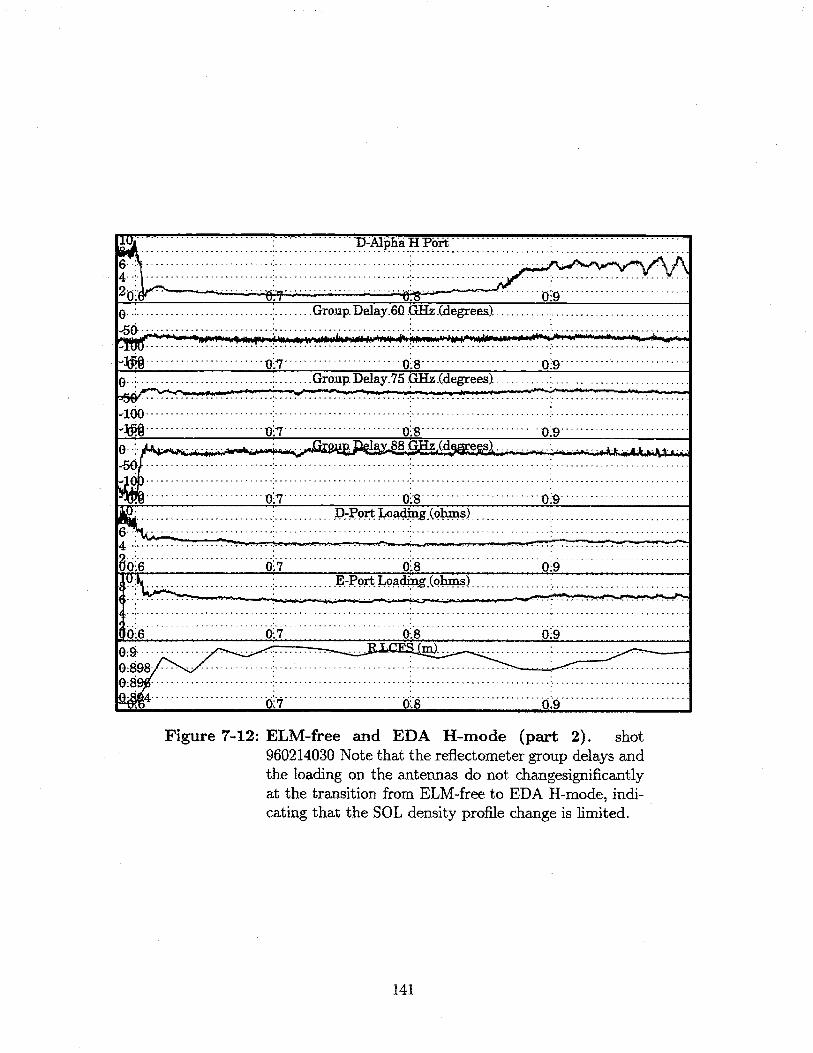
lu --------- ------- --------- I ----------------- D -A lObA H P dft ...........................................
2 --- ------------------------
.... ............. I ................ I ------------------ --------- -------- ------------
4 ... ...... .... ........ .............................. ...... -- ---- ----- I .. .... .............. ... .----------- ------ -- .............................. ........... .0 ..9 ----------
0- ....... ...... ...... Group. Delay_60.6ffi kdegrees) ........ ......... ........... ..... ........ ..... ...... ....... ........... I ......... ......... .... ....... ..... .. .. .....
............. - ...........
.................... * ... 0 .7 0 '.-8 ------------------------ o fq --- .............
........................ ........ Group- Delay_75.GHz.(.degrees) -------............. I .... .... .. ..... ..
'16 0 .......................... ............................ ------ --------- ----------- ............------------------------ 0 :7 --------------- ------- O .S ........... ............ 0 9 1 1 1", -------------- - --------- z I".. ... .. .. .. .. .. .... ... .. ... ..... .. ...I. ... ..... ....... ....... .. .... .. ........ ...... ... ..... ......... .- ....
Q 7 ............... ........ 0 -.8 - ................ 0 :9 - ...... -------------.............. .................. --------- ............ .. .. .. ... ... .... .. ... .. .... ..---- ---
.. . .......4 - .........
.0 "._6 ------ ............... 6 1-6 ---------------------------- --------
------- -- ----------- _ ------- ...........................
................ ................. -------------- ............. - - _ ........10-.6 0:7 0'.8 0,9
.......... ...... M ) ... .... ....... ... ....
............ .. .......... ........ ............... .. ........................... ........... ........... - ._
0-89 0,7 0,'.8 0,9
Figure 7-12: ELM-free and EDA H-mode (part 2). shot960214030 Note that the reflectometer group delays andthe loading on the antennas do not changesignificantlyat the transition from ELM-free to EDA H-mode, indi-cating that the SOL density profile change is limited.
141
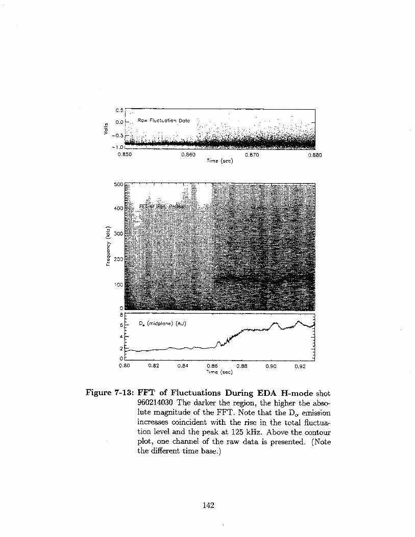
U.5
0.0 Raw Fluctuation Data
0.850 0.860 0.870 0.880Time (sec)
500
400
3 300
C
200
100
0
6 D (midplane) (AU)
4
2
0.80 0.82 0.84 0.86 0.88 0.90 0.92Time (sec)
Figure 7-13: FFT of Fluctuations During EDA .H-mode shot960214030 The darker the region, the higher the abso-lute magnitude of the FFT. Note that the D, emissionincreases coincident with the rise in the total fluctua-tion level and the peak at 125 kHz. Above the contourplot, one channel of the raw data is presented. (Notethe different time base.)
142

5
4 - Centroi Te
32 -I
0.7
6ZS 0.5
0.3-
40C
(D
:3
010
64
0D (midplane) (AU)
0.80 0.82 0.84 0.86 0.88 0.90 0.92Time (sec)
Figure 7-14: EDA H-mode Fluctuation Frequency modulatedby Sawteeth. In this contour plot of the amplitude ofthe Fourier transform of the fast signal from the 88 GHzchannel, the modulation of the peak frequency can beseen. The spikes in the edge ECE signal at 0.02 secondintervals are instrumental.
143
144
Chapter 8
Conclusions and Future Work
8.1 Conclusions
Multi-channel, differential phase reflectometry can provide very accurate electron
density profiles with, depending on plasma conditions, fraction of a millisecond time
response. However, calibration remains a significant challenge due presumably to
multiple reflections in the vacuum chamber before and after a plasma. By calibrating
the reflectometer channels via observed features in the density profile, profile recon-
structions with accuracy of approximately 0.5 cm have been obtained that agree well
with many diagnostics, though not with the TCL It is believed that the discrepancy
between the reflectometer and the TCI can be at least in part attributed to inade-
quately modeled high density plasma outside the LCFS. Fluctuation measurements
with a differential phase reflectometer, though qualitatively useful, are not well suited
to quantitative fluctuation measurements. However, as will be shown in the following
section, some comparatively simple additions to the basic DP receiver will allow for
fluctuation studies using individual sidebands. A comparison of the capabilities of
the three main electron density diagnostics is presented in table 8.1.
Density profiles during many phases of C-Mode plasma operation have been mea-
sured using the differential phase reflectometer. L-H transitions have proven particu-
larly interesting with density gradients of 2 x 10²² m-4 measured 0.5 ms after an L-H
transition. This rapid rise in plasma inventory is in rough agreement with measure-
145
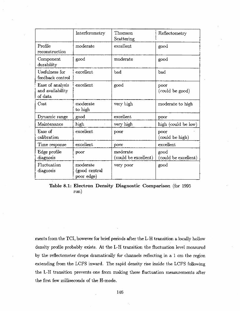
Table 8.1: Electron Density Diagnostic Comparison (for 1995run)
ments from the TCI, however for brief periods after the L-H transition a locally hollow
density profile probably exists. At the L-H transition the fluctuation level measured
by the reflectometer drops dramatically for channels reflecting in a 1 cm the region
extending from the LCFS inward. The rapid density rise inside the LCFS following
the L-H transition prevents one from making these fluctuation measurements after
the first few milliseconds of the H-mode.
146
Interferometry Thomson ReflectometryScattering
Profile moderate excellent goodreconstruction
Component good moderate gooddurability
Usefulness for excellent bad badfeedback control
Ease of analysis excellent good poorand availability (could be good)of data
Cost moderate very high moderate to highto high
Dynamic range good excellent poor
Maintenance high very high high (could be low)
Ease of excellent poor poorcalibration (could be high)
Time response excellent poor excellent
Edge profile poor moderate gooddiagnosis (could be excellent) (could be excellent)
Fluctuation moderate very poor gooddiagnosis (good central
poor edge)

8.2 Future Reflectometry Work
The success of this thesis and the need for more detailed knowledge of the electron
density profile in C-Mod warrant an aggressive approach to further reflectometry
developmenta. However, the current funding and manpower shortages on the C-Mod
experiment place a limit on what experiments can be done. The following actions are
recommended, assuming the current staffing arrangementb and the continued interest
in studies of enhanced confinement modes of operation.
8.2.1 Reliability Improvement and Maintenance Reduction
The reflectometer was developed as an experimental diagnostic and as a graduate
student thesis project. As might be expected some aspects bear the shortcomings of an
initially less than polished design and many late night modifications. The wiring and
hardware are currently being streamlined by a graduate student and a staff engineer.
In addition to general straightening up of the experimental rack several upgrades are
needed. The Gunn oscillators should be stabilized such that their IF drifts less than
1 MHz. This will reduce the need to tune the system in the morning before each
run day and is essential for the instrumentation described in § 8.2.6 for fluctuation
diagnosis. The mica vacuum windows should be replaced with a more rugged design.
Quite probably a simple glass window will suffice though the transmission needs to be
tested. At the same time, an improved technique should be developed for installing
and removing the waveguides from the narrow reentrant vacuum port. In addition,
all other experiments using triggers from the reflectometer CAMAC crate should
receive their trigger through a fiber rather than direct cable connection to reduce the
possibility of damage to sensitive equipment due to ground loops.
The analysis software can benefit from similar attention. In particular, data re-
duction and profile inversion requires far more operator input in fringe jump detection
aThis section is intended not only as a the author's suggestion of how to develop refiectometry,but also as a memo to the C-Mod scientific staff regarding what work is needed for the diagnostic'scontinued use on C-Mod.
'A single graduate student working under the guidance of a staff scientist with occasional helpfrom the engineering and technical staff
147
than it should. The author will attempt the software upgrades some time after this
thesis is complete to simplify this process. Also, dropping the upconversion frequency
from 500 to 350 MHz could significantly simplify the the fringe jump correction rou-
tine. This upgrade is also needed for following PEP mode profile evolution.
8.2.2 Calibration and Profile Reconstruction
Probably the biggest issue with the current system is the difficulty in calibrating
the diagnostic. A movable calibration plate mounted on a rod such that it can be
moved radially should do much to alleviate this problem. Figure 8-1 is a sketch of
the proposed calibration assembly. Also, installing absorbing structures on both sides
of A-port would reduce the multiple reflections that are assumed to be the cause of
calibration difficulties. These upgrades should allow improvement in the reliability
and accuracy of the diagnostic. However, obtaining scale length measurements on
the order of 1 mm as is desired for studying balooning mode stability limits during
H-modes, for example, is probably beyond the capabilities of the diagnostic as cur-
rently configured. Resolution of that range will require greater care with respect to
amplitude to phase modulation, the beam patterns of the launching horns, and the
ray tracing of the launched waves.
8.2.3 Cross Calibration Profile
As has been stated before, the other density diagnostics also have serious shortcomings
and strengths. The Thomson scattering diagnostic in particular is difficult to keep
calibrated between shutdowns. However, TS is the only diagnostic with the potential
resolution and dynamic range currently requested. Standard C-Mod operation calls
for one or two "fiducial" shots per run day. These have a standard set of control
inputs and are intended to monitor the day-to-day condition of the machine walls by
monitoring impurity levels, radiated power fraction, and L to H transition thresholds.
A similar fiducial for diagnostic cross calibration would also be useful. In particular,
a slow ramp in the electron inventory through a central density of 1.5 x 10²⁰ m-
148

717
&Olbration Plate \0,
Microwave AbsorbeMicrowave Horns~
Calibration Plate,(retracted)
Bellows
Figure 8-1: Proposed Calibration Paddle
would allow for an accurate cross calibration between the Thomson scattering and
the reflectometer. This should be performed in L-mode at low to modest current to
ensure that the density profile is peaked on axis and that the sawteeth are small. The
ramp in density must be slow enough to allow for sufficient laser pulses to minimize
the random error in the Thomson scattering measurement due to photon statistics.
It is expected that a diagnostic fiducial can either be incorporated into the current
fiducial shot or be performed on a weekly or bi-weekly basis so as not to overburden
the run schedule.
In addition, there exists a significant gap in the reflectometer density coverage
between 0.95 and 1.5 x 10 2 0 m-3 (88 and 110 GHz) that compromises the profile
inversion of the reflectometer. For this calibration scheme to be accurate to 5%, at
least one more frequency is needed. This can be accomplished by adding a complete
channel (both millimeter and rf components) at 100 GHz or by applying the technique
suggested in § 8.2.5. Either of these will require substantial funds (- $10,000 to
$20,000), however, a robust TS calibration technique is well worth this expense.
149

8.2.4 X-Mode Polarization
The least expensive option to extend the density range of the reflectometer is to rotate
the polarization to X-mode and study the group delay to the LHC. This approach will
allow for access central densities of 4.5 x 10 20m- 3 at 7.9 tesla using the frequencies we
currently have available (see Fig. 4-7). This should be particularly interesting for PEP
mode studies. For 5.3 tesla H-modes, pedestal heights up to 2.3 x 10²⁰ m-3 can be
studied (see Fig. 4-5). This is a 50% increase over current capabilities and will allow
the diagnostic to see beyond the SGR for some H-mode shots. However, pedestal
heights of 3.5 x 10²⁰ m-3 have been measured by ECE cutoff, so for many if not most
H-modes the problem of only being able to probe to the SGR will probably continue.
In addition, there are some complications that need to be addressed. First, along the
way to the X-mode cutoff, the beam will have to pass the 0-mode cutoff. Because
the 0-mode cutoff comes first, signal reflected from this cutoff has the potential to
corrupt the group delay measurements far more than the X-mode cutoff can corrupt
our current 0-mode measurements. The current horns do not allow for adjustment
of the launch angle to match the field pitch at the plasma boundary. A set of scalar
horns would allow for this rotation based on the expected current and toroidal field
for the day's experiments. Getting the polarization correct for all shots during a run
will probably be impossible. However, it may be possible to estimate the fraction
of the power going into each mode by observing the cutoffs during the plasma ramp
up and ramp down. Second, the group delay will be considerably more than with
the current 0-mode system. This will probably necessitate reducing the modulation
frequency by as much as a factor of four. Third, there is the issue of what the
highest useable frequency is. As shown in Fig. 4-6, even a small electron density
behind the limiter can cause significant separation between the upper cutoff and the
upper hybrid resonance. This prevents access to the left hand cutoff at 5.3 tesla for
frequencies above 90 GHz. Lastly, it should be pointed out that unlike the right hand
wave, the left hand wave is more sensitive to hollow profiles than the O-mode. This
cNote that toroidal field ripple is significant at the horn location dropping the B-field by 10percent over a 1/R dependance.
150
can be seen by looking at figure 4-5. (Moving from right to left, the LHC X-mode
curves slope up while the RHC X-mode curves slope down.) The location of the
cutoff layer is the intersection of the plasma density profile with the curves shown. So
while rotating the polarization will improve the dynamic range of the reflectometer,
given the flat to hollow profiles it will not change the reflectometer into a core density
diagnostic.
8.2.5 More Sophisticated Modulation Techniques
There are many modulation techniques that one can envision. Several groups (????)
have been developing pulsed reflectometry techniques. With the millimeter wave
hardware in hand at present, such techniques should be simple to implement. Another
option that may prove useful is putting multiple modulation signals in the upconvertor
as shown in Fig. 8-2. By using two or more upconversion frequencies, multiple group
delay measurements can be derived from one set of millimeter wave components.
This could be especially useful for an LHC X-mode diagnostic where the separation
in critical density between oscillator frequencies is greater than in O-mode. The
upconversion frequencies shown are arbitrarily chosen, and again for LHC X-mode
the 1 GHz IF should probably be reduced to 250 MHz. The input power to the
upconvertor is limited and the upconversion efficiency drops as the power is reduced,
so the number of upconversion frequencies will be limited. Multiple data points could
be achieved via a swept or multiplexed upconversion signal.
8.2.6 Fluctuation Diagnostics
So far the reflectometer has been used primarily as a density profile diagnostic and
studies of fluctuations have been limited to very qualitative ones. For comparisons
with reflectometers elsewhere and to measure Doppler shifts due to plasma rotation, a
single sideband of a reflectometer channel should be studied independently. Figure 8-3
shows the modifications needed to the current reflectometer to observe one sideband.
The rotation of perturbations in the density near the critical layer will Doppler shift
151

4 GHz 3 GHz
91 908384
87 GHzGKz ISO ISO To Plasma
87.25GHz
1 GHz
From Plasma
Pr mp
4.25 3.25 3.75 2.75GHz GHz GHz GHz
1 GHz
TO PHASE DETECTORS
Figure 8-2: Multiple Upconversion Frequency Concept. By us-ing multiple upconversion frequencies, several group delaymeasurements chan be performed with a single millimeterwave transmitter and receiver.
152
the returned signal. This will give a crude measure of the plasma rotation velocity.
In no way should such a measurement alleviate the need for spectroscopic rotation
measurements during H and PEP mode studies. However, the time response for the
reflectometer for such measurements can be on the order of tens of microseconds, so
such a rotation measurement may provide some insight into the sequence of events
during L to H transitions for example. Placing a receiving horn well off the midplane
will improve the sensitivity to rotation. PEP mode studies at 7.9 tesla using X-mode
polarization should prove particularly interesting as the 110 GHz channel will be able
to reach the region where the internal confinement barrier is expected to be.
A key interest of turbulence modelers is the correlation length of the fluctuations
that drive turbulence. The multiple upconversion concept sketched in Fig. 8-2 lends
itself well to measuring this. By correlating the sidebands from multiple modulation
frequencies, the correlation length can be mapped out provided the density gradient
is also measured. All of these investigations will require developing an improved
raytracing code or application of a two or three dimension full wave code such as the
one developed by Irby [79]. Lenses to focus the launched and returned beam may also
be needed to improve k resolution. The effect of modifying the launching antennas
should be investigated using the codes described above.
8.3 More Ambitious Upgrades
8.3.1 ICRF Loading Studies
Another potential application of reflectometry on C-Mod would be the study of the
plasma directly in front of the ICRF antennas. In O-mode, frequencies of interest
would be 10 to 30 GHz. These frequencies can be transmitted via coaxial cable, so
a complicated waveguide run could be avoided and access could be provided via a
vertical port. There is enough room to fit a microstrip patch antenna on the wall
between the two pairs of two strap antennas. Here reflections from the edges of the
ICRF antennas is probably inevitable, however, by eliminating the nonlinear gain
153

500 Mhz fromoscillator box
50 60 GHz in
GHz ISO ISO To PlasmaHz
65 MHz
35 MHZ
50.035GHz GSO From Plasma
535 MHz ,r m
535 &465 Mhz
SE DETECTORS To DP receiver
Figure 8-3: Suggested Modifications for Single SidebandStudy. This approach eliminates the need to phase lockthe launching and receiving sources by referencing the re-ceived signal to the 30 MHz oscillator [80]. The 65 MHzfilter needs to be sufficiently narrow to eliminate 60 and 70MHz generated in the mixer. This filter also sets a limitto the bandwidth of the 35 MHz IF between the two Gunnoscillators. Changing the modulation frequency from 500MHz to something lower would allow for increased band-width for the Gunn IF.
154
565 MHz
30MHz
TO PHA

amplifiers in the DP receiver, these extra reflections can be zeroed out at the phase
detector.
8.3.2 Eliminating Limiter Effects
While the limiter has proven useful for calibration, it greatly modifies the SOL. To
eliminate this problem making the reflectometer measurements more useful for di-
vertor modelers, the horns could be positioned off of the midplane either below or
above the limiter. This will eliminate the symmetry provided by midplane launch
and will necessitate a flux mapping provided by EFIT to interpret the data. On
the other hand, moving the launching horns to an off axis location will improve the
profile reconstruction accuracy with respect to flux surfaces, as there is considerable
flux expansion as one moves away from the midplane.
Moving the limiter is also a possibility. Plans for the tangentially viewing inter-
ferometer call for at least part of the limiter to be removed. Moving the horns to
another port is extremely unlikely due to the limited diagnostic space available.
8.3.3 Higher Frequencies
A severe limitation to the current diagnostic is operating frequency. The frequencies
available limit measurements to 1.5 x 10 2 0 m-3 while current high recycling H-Modes
now have densities as high as 3.5 x 10 20m- 3 within a few centimeters of the LCFS.
At 5.3 Tesla, cyclotron absorption greatly limits operation from 115 to 125 GHz.
The next window, from 125 to 220 GHz would allow the study of densities from
1.9 x 10²⁰ to 6 x 10²⁰ m-3 . Millimeter wave equipment becomes quite expensive
over 110 GHz, but the work demonstrated in this thesis and elsewhere [48} provided
sufficient confidence that either an O-mode system for frequencies above 125 GHz or
an X-mode system from 170 to 230 GHz will work. Such a project may be well suited
for collaborations perhaps performed under an SBIR.
The other option is to arrange for high field launch to the LHC. The millimeter
wave equipment for such a reflectometer is already available in the current O-mode
155

system. The thin inner wall protection tiles (~ 1.5 cm thick) make the threading of
transmitting and receiving lines to the midplane on the inner wall a daunting task,
not to mention developing antennas.
8.4 Future H-Mode Work
It is not altogether clear what the long range goals for C-Mod should be with respect
to H-mode development. C-Mod has already contributed greatly to the scaling of L
to H transitions. With the boronization of the vacuum chamber, H factors in excess
of 2.5 have been achieved which is comparable to the values achieved elsewhere in
ELM-free H-Mode. To continue improving the H-factor, VH-modes will probably be
needed. To get VH-modes some method of off axis current drive will be needed. The
planned four strap ICRF antenna will provide this capability.
Controlling the density rise during ELM-free H-modes is another issue. Divertor
pumping may help in achieving lower density EF H-modes. Currently a prototype
divertor cryopump is in place and ready for testing during the spring 1997 run cam-
paign.
From the point of view of understanding H-mode physics, several diagnostics are
needed. Currently, the plasma current profile and the edge toroidal and poloidal
rotation are not measured. The diagnostic neutral beam should help in determining
all of these quantities. In addition, the views for the current UV spectrograph [81]
are being modified to look for doppler shifts due to plasma rotation. If these efforts
prove successful, Doyle [62, 82] has demonstrated that with good poloidal rotation
measurements and high shear in the rotation velocity, quite good spatial resolution
can be inferred from collective scattering diagnostics. Stated another way, without
good knowledge of the plasma rotation velocity all frequency measurements have an
error bar corresponding to k -ve which can be far in excess of the natural frequency
spread in the fluctuations, making the measurement quantitatively useless.
156
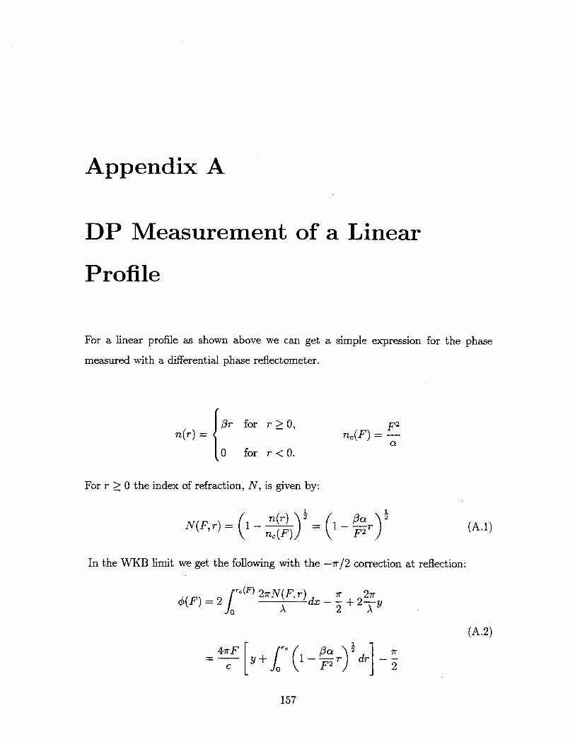
Appendix A
DP Measurement of a Linear
Profile
For a linear profile as shown above we can get a simple expression for the phase
measured with a differential phase reflectometer.
3r for r > 0,
0 for r < 0.
F 2n,(F) =
For r > 0 the index of refraction, N, is given by:
n (r)n' (F)
O3a2 r )
I2
(A.1)
In the WKB limit we get the following with the -7r/2 correction at reflection:
() (F) 27rN F, r) -r 27rO(F) =2 2 lr(Frdx 2 +2-
_47rF
C
(A.2)
y-
157
N(F, r) = I
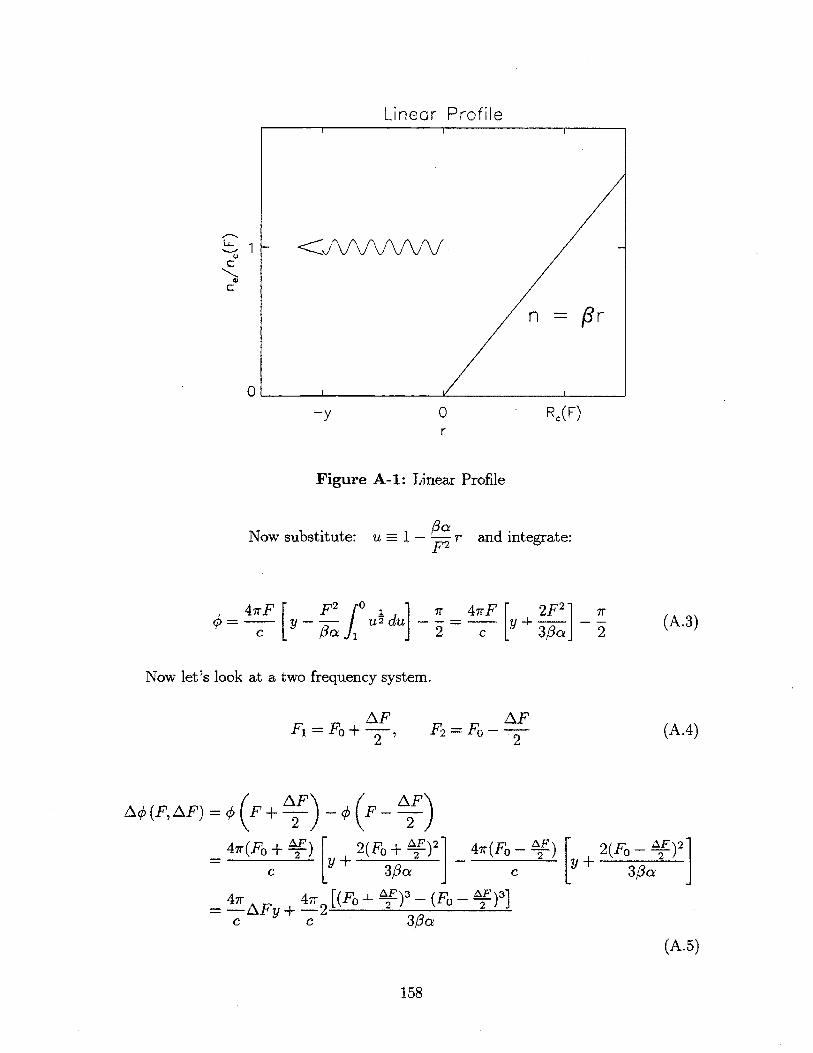
Linear Profile
0r
R (F)
Figure A-1: Linear Profile
Now substitute: U 10- and integrate:
4-irFC
y - f u du
Now let's look at a two frequency system.
AFF1 =Fo+ 2 ,
F AF)
47r(Fo + ") 2(Fo + )2] 47r(Fo2 y + 32a
= A y 2[(F0 + A)33_ (Fo - )3]47rAFy +-42 23J 3 _QC C30
(A.5)
158
I-
0
<AW&VW
n f r
47C1
[y(A.3)
(A.4)F2=Fo-AFF2=F 2
=4F+ 2 ,)A 0(F, AF)
- ) 2(Fo - II)2~2 y + 3 2

Now make the approximation F0 > AF:
AF 3 _ (F AF) 3 2AP3Fo+2 - 0- 3FF2 2 4 (A.6); 3AFF 2
Substituting in gives the rather simple result:
47rA (Fo, AF) = -AF [y + 2Rc(F)j
r F 2 (A.7)= -AF y+2-
C 1 0
A couple of interesting features of this result are: first, the phase measurement
is proportional to the modulation frequency. One can unfortunately gain no more
information about a linear density profile by changing the modulation frequency. In
addition, since the largest contributions to the group delay for most expected profiles
are the location of the reflecting layer and the slope in the region near that reflecting
layer, under most conditions no great improvement in profile reconstruction can be
expected by using multiple modulation frequencies.
Second, the ultimate resolution of a reflectometer will be the absolute error in
the phase measurement. The amplitude to phase modulation specifications can be
relaxed by increasing the modulation frequency. For example, the phase error over
the dynamic range of the limiting amps used in the C-Mod reflectometer is ±2.5 deg.
In order to obtain ±2 mm resolution one needs a modulation frequency of I Ghz.
Third, this simple result points to a second approach to profile inversion. By
assuming the profile is piecewise linear and monotonic one can construct a matrix
equation relating R as a function of n. This approach has the added advantage of
providing a method of including errors, point measurements, and constraints in the
inversion. Figure A-3 shows how a profile might be linearized. The following tour de
force of LaTex will show what should be obvious, that the group delay measured by
each reflectometer channel can be put into a form <bi = E ayxj.
159

~Ii/
/ II,///p
I/Il'II
/ // I
/ / // / I
I I/ // / I
/ / II F
A.
vv~/~v~
/ /
rFigure A-2: Indistinguishable Profiles To a single frequency DP
reflectometer, all of the profiles shown above give thesame returned signal.
160
2H
0
*40H
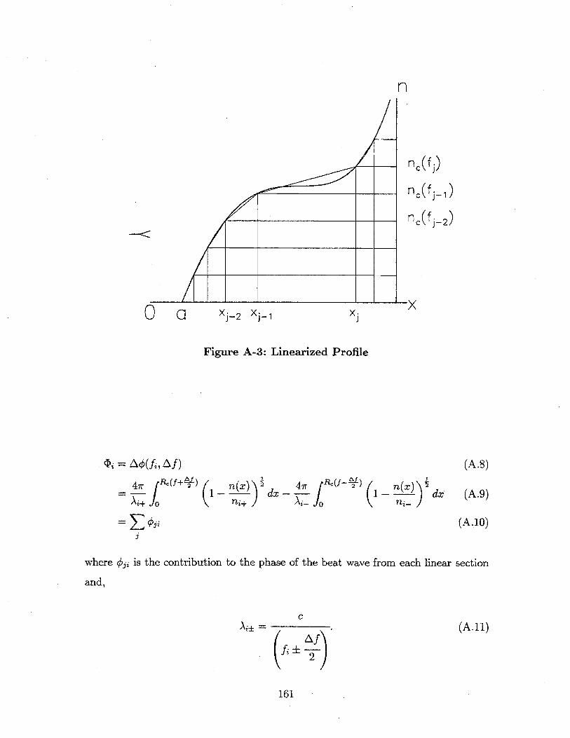
/
x.Xj- 2 Xj-1
Figure A-3: Linearized Profile
<= =q4(f ,ALf)
47r 2f+%)
Aj+ 10
= S qOi
(1 n(x) 2 dni+ /
where Oji is the contribution to the phase of the beat wave from each linear section
and,
C
=
(A.11)
161
n
QaO
(A.8)
(A.9)
(A.10)
nc(f _1)
n,(fj-2)
ni-
47r R(- 3
Aj- 0

Writing Oji explicitly gives:
47r f+* Ni+(x)dx - ' fj ' N_(x)dx
4ir f *o N+(x)dx - R' Ni_(x)dx
fi+ Ni+(x)dx - f'- Ni_(x dx
47 Rf+ Ni+(x)dx
if nx+1 < n,+
if n3 < n_ < ni+1 < n,+
if n< _ rnc-< nfl < nj+1
if nc_ <n< n < n+l
if nog ; nj
(A.12)
where,
nc AfncaE e(fi 2 )
Nia(x) = (I n(x)njia
and R.± = Re: (f
and Nja(n) = 1 - -)ni±
Now change the variables of integration,
dNia 1 1dn 2ni± N
and dn = fl - njdx x,+ 1 - xj
and integrate
1 b Ni±(b)Ni dx = N a
-2ni j'+1 - x3 Ni+ (b)
nj+l - na JNi (a)
= 2ni± xj+1 - xj [N3s(b) - Nia(a)]3 nj+1 - n
finally giving
Oji = (x3+1 - x3) O3.j
162
Oji = 4
0
dNi dn ~N i ] dNi (A.13)
(A.14)
(A.15)
(A.16)
N (n) - - Ni (nj) + N_(nj+1)
N?,(nj) - Ni+(nj+1) - Ni_ (n,) + 0
NZ+(nj) - 0 - Ni_ (nj) + 0
NZ+(n.) - 0 - 0 + 0
0
if n.+, < n+
if nj < n,- < nj+1 < nci+
if nj < n, < n, < nj+1
if n,_ < n < n, < nj+l
if n., ; n,
K M 2n ,3(nj+1 - nj)
b -xo000 + (-%, + u(j-10)) Xj
j=0
r=-0 for i=0
wh re - # 3i for i > 0
A point density measurement or constraint, n, at x can be included with:
(n - nj)xj+1 + (nj+1 - n)x, = (nj+1 - nj)x.
Multiple constraints can be represented by a matrix equation:
C.X.=Q
163
where:
(A.17)
(A.18)
(A.19)
(A.20)
(A.21)
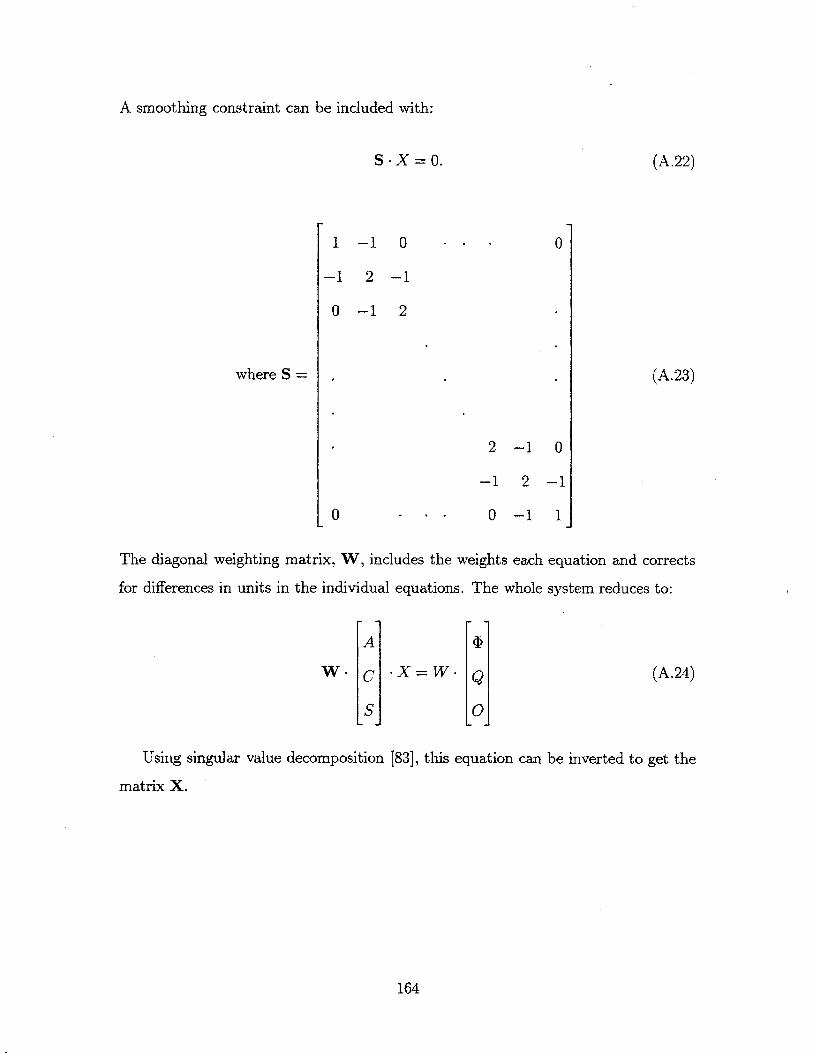
A smoothing constraint can be included with:
S -X = 0.
where S =
1 -1 0
-1 2 -1
0 -1 2
0
The diagonal weighting matrix, W, includes the weights each equation and corrects
for differences in units in the individual equations. The whole system reduces to:
W.A
C
S
.X=W. Q0
(A.24)
Using singular value decomposition [83], this equation can be inverted to get the
matrix X.
164
(A.22)
0
0
-1
1
(A.23)
2 -1
-1 2
0 -1

Appendix B
List of Acronyms
Acronym Meaning First Usage
D-Alpha Emission from the cc line of Deuterium page 34Emission
DP Differential Phase page 76
ECE Electron Cyclotron Emission page 48
EDA Enhanced Da page 139
EF Equilibrium Field (Coils) page 41
ELM Edge Localized Mode page 34
FSR Fluctuation Suppression Region page 130
GPC Grating Polychromator page 49
H-Mode High Confinement Mode page 33
ICRF/ ICRH Ion Cyclotron Resonance page 50Frequency/Heating
Table B.1: List of Acronyms
165
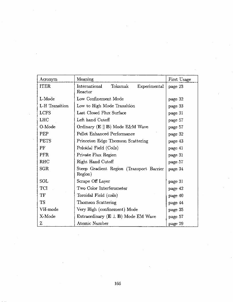
Acronym I Meaning I First Usage
ITER
L-Mode
L-H Transition
LCFS
LHC
O-Mode
PEP
PETS
PF
PFR
RHC
SGR
SOL
TCI
TF
TS
VH-mode
X-Mode
z
International Tokamak ExperimentalReactor
Low Confinement Mode
Low to High Mode Transition
Last Closed Flux Surface
Left hand Cutoff
Ordinary (E 11 B) Mode E&M Wave
Pellet Enhanced Performance
Princeton Edge Thomson Scattering
Poloidal Field (Coils)
Private Flux Region
Right Hand Cutoff
Steep Gradient Region (Transport BarrierRegion)
Scrape Off Layer
Two Color Interferometer
Toroidal Field (coils)
Thomson Scattering
Very High (confinement) Mode
Extraordinary (E I B) Mode EM Wave
Atomic Numbera _________________________________________________ L
166
page 23
page 32
page 33
page 31
page 57
page 57
page 32
page 43
page 41
page 31
page 57
page 34
page 31
page 42
page 40
page 44
page 35
page 57
page 29
Bibliography
[1] S.M. Kaye and R Goldston. Nuclear Fusion, 25:65, 1985.
[2] R. D. Stambaugh et al. Enhanced confinement in tokamaks. Phys. Fluids B,2(12):2941, December 1990.
[3] F. Wagner et al. Regime of improved confinement and high beta in neutral-beam-heated divertor discharges of the ASDEX tokamak. Phys. Rev. Lett., 49:1408,1982.
[4] Francis F. Chen. Introduction to Plasma Physics and Controlled Fusion, vol-ume 1. Plenum Press, 2 edition, 1984.
[5] John Wesson. Tokamaks. Oxford University Press, 1987.
[6] Martin Schwarzschild. Structure and Evolution of the Stars. Dover Publications,Inc., 1958.
[7] J.D. Lawson. Some criteria for a power producing thermonuclear reactor. Pro-ceedings of the Physical Society B, 70(6), 1957.
[8] I.H.Hutchinson. Personal Communication, 1996.
[9] Darren Thomas Garnier. Lithium Pellet Injection Experiments on the AlcatorC-Mod Tokamak. Ph.D. thesis, Massachusetts Institute of Technology, June 1996.
[10] P.N. Yushmanov. Scalings for tokamak energy confinement. Nucl. Fusion,30(10):1999, 1990.
[11] R. J. Groebner. An emerging understanding of H-mode discharges in tokamaks.Phys. Fluids B, 5(7):2343-2354, July 1993.
[12] S. M. Kaye (Chairman). Papers from the 5th IAEA technical committee meeting/US-Japan workshop on H-mode physics. Plasma Phys. and Control. Fusion,38(8):1089-1501, August 1996.
[13] D. J. Ward. LH transition theories and theory of H-mode. Plasma Phys. Control.Fusion, 38:1201-1212, 1996.
167
[14] Ian H. Hutchinson and Miklos Porkolab. Alcator C-Mod fusion research program1996-2000. Technical report, MIT Plasma Fusion Center, 175 Albany Street,Cambridge, MA 02139, June 1995.
[15] E. S. Marmar. The Alcator C-Mod diagnostic complement. Rev. Sci.Instrum,63:4695, October 1992.
[16] James Reardon et al. Spatial structure of pump wave and parametric decayinstability during ICRF injection on Alcator C-Mod. Bulletin of the AmericanPhysical Society, October 1996.
[17] D. Dimock, B. Grek, D. Johnson, B. LaBombard, B. Lipschultz, and G. Mc-Cracken. A compact thomson scattering system. Rev. Sci. Instrum, Jan 1997.
[18] J. H. Irby et al. Prototype tangential interferometer for Alcator C-Mod. InBulletin of the American Physical Society, volume 41, page 1551, October 1996.
[19] T. Luke. Measurement of Particle Transport Coefficients on Alcator C-Mod.Ph.D. thesis, Massachusetts Institute of Technology, October 1994.
[20] B. Labombard. Scaling and transport analysis of divertor conditions on theAlcator C-Mod tokamak. Phys. Plasmas 2, pages 2242-2248, 1995.
[21] L. L. Lao et al. Reconstruction of current profile parameters and plasma shapesin tokamaks. Nuclear Fusion, 25, 1985.
[22] R.S. Granetz, I.H. Hutchinson, J. Gerolamo, W. Pina, and C. Tsui. Magneticdiagnostics in Alcator C-Mod. Rev. Sci. Instrum., 61:2967, 1990.
[23] T.S. Hsu. The Submillimeter Wave Electron Cyclotron Emission Diagnostic forthe Alcator C-Mod Tokamak. Ph.D. thesis, Massachusetts Institute of Technol-ogy, 1993.
[24] Amanda Eileen Hubbard. Measurement of Electron Density on JET by Mi-crowave Reflectometry. Ph.D. thesis, Imperial Collage of Science and Technology,May 1987.
[25] J.L. Terry et al. The visible, imaging diode arrays on Alcator C-Mod. Rev. Sci.Instrum., 66(1), January 1995.
[26] C. Kurz. Ph.D. thesis, Massachusetts Institute of Technology, 1995.
[27] R. Parker et al. Nucl. Fus., 25:1985, 1985.
[28] M. Greenwald et al. Phys. Plasmas, 6(2):2308, 1995.
[29] J. Goetz et al. Comparison of detached and radiative divertor operation inAlcator C-Mod. Phys. Plasmas, 3(5):1908-15, May 1996.
168
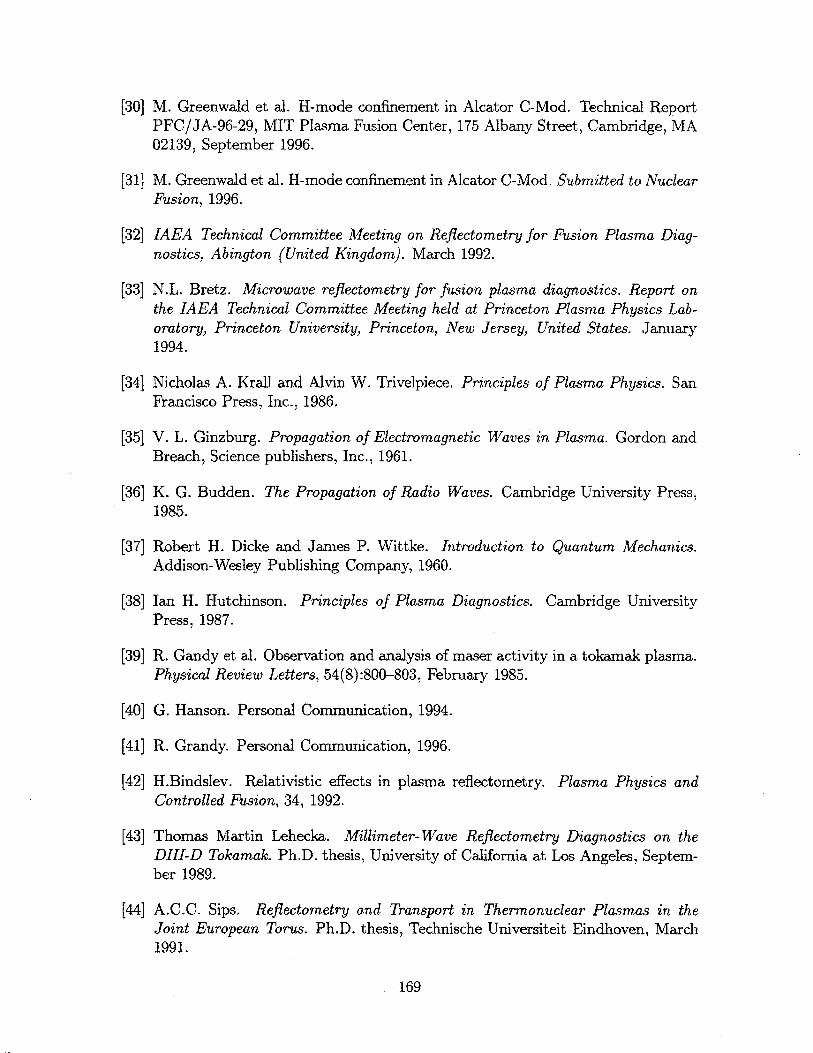
[30] M. Greenwald et al. H-mode confinement in Alcator C-Mod. Technical ReportPFC/JA-96-29, MIT Plasma Fusion Center, 175 Albany Street, Cambridge, MA02139, September 1996.
[31] M. Greenwald et al. H-mode confinement in Alcator C-Mod. Submitted to NuclearFusion, 1996.
[32] IAEA Technical Committee Meeting on Reflectometry for Fusion Plasma Diag-nostics, Abington (United Kingdom). March 1992.
[33] N.L. Bretz. Microwave reflectometry for fusion plasma diagnostics. Report onthe IAEA Technical Committee Meeting held at Princeton Plasma Physics Lab-oratory, Princeton University, Princeton, New Jersey, United States. January1994.
[34] Nicholas A. Krall and Alvin W. Trivelpiece. Principles of Plasma Physics. SanFrancisco Press, Inc., 1986.
[35] V. L. Ginzburg. Propagation of Electromagnetic Waves in Plasma. Gordon andBreach, Science publishers, Inc., 1961.
[36] K. G. Budden. The Propagation of Radio Waves. Cambridge University Press,1985.
[37] Robert H. Dicke and James P. Wittke. Introduction to Quantum Mechanics.Addison-Wesley Publishing Company, 1960.
[38] Ian H. Hutchinson. Principles of Plasma Diagnostics. Cambridge UniversityPress, 1987.
[39] R. Gandy et al. Observation and analysis of maser activity in a tokamak plasma.Physical Review Letters, 54(8):800-803, February 1985.
[40] G. Hanson. Personal Communication, 1994.
[41] R. Grandy. Personal Communication, 1996.
[42] H.Bindslev. Relativistic effects in plasma reflectometry. Plasma Physics andControlled Fusion, 34, 1992.
[43] Thomas Martin Lehecka. Millimeter-Wave Reflectometry Diagnostics on theDIII-D Tokamak. Ph.D. thesis, University of California at Los Angeles, Septem-ber 1989.
[44] A.C.C. Sips. Reflectometry and Transport in Thermonuclear Plasmas in theJoint European Torus. Ph.D. thesis, Technische Universiteit Eindhoven, March1991.
169
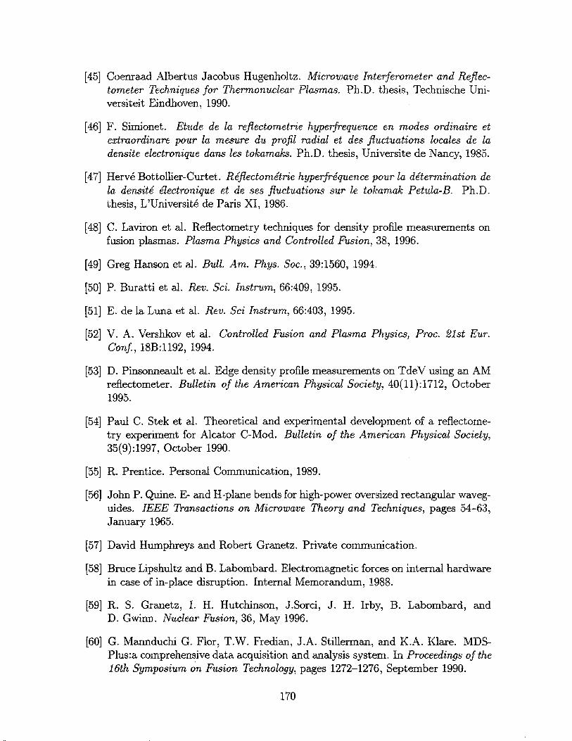
[45] Coenraad Albertus Jacobus Hugenholtz. Microwave Interferometer and Reflec-tometer Techniques for Thermonuclear Plasmas. Ph.D. thesis, Technische Uni-versiteit Eindhoven, 1990.
[46] F. Simionet. Etude de la reflectometrie hyperfrequence en modes ordinaire etextraordinare pour la mesure du profil radial et des fluctuations locales de ladensite electronique dans les tokamaks. Ph.D. thesis, Universite de Nancy, 1985.
[47] Herv6 Bottollier-Curtet. Riflectomitrie hyperfriquence pour la determination dela densitie' lectronique et de ses fluctuations sur le tokamak Petula-B. Ph.D.thesis, L'Universit6 de Paris XI, 1986.
[48] C. Laviron et al. Reflectometry techniques for density profile measurements onfusion plasmas. Plasma Physics and Controlled Fusion, 38, 1996.
[49] Greg Hanson et al. Bull. Am. Phys. Soc., 39:1560, 1994.
[50] P. Buratti et al. Rev. Sci. Instrum, 66:409, 1995.
[51] E. de la Luna et al. Rev. Sci Instrum, 66:403, 1995.
[52] V. A. Vershkov et al. Controlled Fusion and Plasma Physics, Proc. 21st Eur.Conf., 18B:1192, 1994.
[53] D. Pinsonneault et al. Edge density profile measurements on TdeV using an AMreflectometer. Bulletin of the American Physical Society, 40(11):1712, October1995.
[54] Paul C. Stek et al. Theoretical and experimental development of a reflectome-try experiment for Alcator C-Mod. Bulletin of the American Physical Society,35(9):1997, October 1990.
[55] R. Prentice. Personal Communication, 1989.
[56] John P. Quine. Fr and H-plane bends for high-power oversized rectangular waveg-uides. IEEE Transactions on Microwave Theory and Techniques, pages 54-63,January 1965.
[57] David Humphreys and Robert Granetz. Private communication.
[58] Bruce Lipshultz and B. Labombard. Electromagnetic forces on internal hardwarein case of in-place disruption. Internal Memorandum, 1988.
[59] R. S. Granetz, I. H. Hutchinson, J.Sorci, J. H. Irby, B. Labombard, andD. Gwinn. Nuclear Fusion, 36, May 1996.
[60] G. Mannduchi G. Flor, T.W. Fredian, J.A. Stillerman, and K.A. Klare. MDS-Plus:a comprehensive data acquisition and analysis system. In Proceedings of the16th Symposium on Fusion Technology, pages 1272-1276, September 1990.
170
[61] Thomas Lehecka. Personal Communication, 1989.
[62] Edward Doyle et al. Physics of turbulence control and transport barrier formationin DIII-D. In 16th IAEA Fusion Energy Conference (Montreal), number F1-CN-64/AP2-11, October 1996.
[63] P.C. Stangeby and G.C. McCracken. Plasma boundary phenomena in tokamaks.Nucl. Fus., 30(7):1225, 1990.
[64] P.C. Stangeby. The interpretation of plasma probes for fusion experiments. InOrlando Auciello and Daniel L. Flamm, editors, Plasma Diagnostics, volume 2.Academic Press, 1989.
[65] B. Labombard. Personal Communication, 1997.
[66] G F Matthews et al. J. Nucl. Mater., 1986.
[67] A.E. Hubbard et al. Local plasma parameters and H-mode threshold in AlcatorC-Mod. In 16th IAEA Fusion Energy Conference (Montreal), number F1-CN-64/AP2-11, October 1996.
[68] A. Hubbard. Personal Communication, 1997.
[69] S. Wolfe. Effect of edge current on flux reconstruction in Alcator C-Mod. InBulletin of the American Physical Society, volume 41, page 1482, October 1996.
[70] Yuichi Takase. Personal Communication, 1997.
[71] John Rice. Personal Communication, 1997.
[72] D. Veron. Opt. Comm., 10:95, 1974.
[73] E. Mazzucato and R. Nazikian. Radial scale length of turbulent fluctuations inthe main core of TFTR plasmas. Phys. Rev. Lett., 71(12):1840-1843, September1993.
[74] E. S. Marmar et al. Boronization on Alcator C-Mod. In Bulletin of the American
Physical Society, volume 41, page 1551, October 1996.
[75] C. Reddy et al. The Alcator C-Mod boronization system. In Bulletin of theAmerican Physical Society, volume 41, page 1551, October 1996.
[76] J.E. Rice et al. Impurity transport in Alcator C-Mod plasmas. Physics of Plas-mas, to be published, June 1997.
[77] I.H.Hutchinson et al. Fast edge mode observed during enhanced D, phase inAlcator C-Mod. In Bulletin of the European Physical Society, 1997.
[78] I.H.Hutchinson. Personal Communication, 1997.
171

[79] J. H. Irby et al. 2D full wave simulation of ordinary mode refiectometry. PlasmaPhysics and Controlled Fusion, 25(5), May 1993.
[80] J.L. Doane. Broadband superheterodyne tracking circuits for millimeterwavemeasurements. Review of Scientific Instruments, 51(3):317, Mar 1980.
[81] B. L. Welch et al. High-resolution visible/ultraviolet measurements from theAlcator C-Mod tokamak. Bull. Am. Phys. Soc., 41, November 1996.
[82] Edward Doyle et al. Bull. Am. Phys. Soc., 1995.
[83] William H. Press et al. Numerical Recipes in C. Cambridge University Press,1988.
172