regeneration, local dimension, and …jhauenst/preprints/hauenstein_thesis.pdf · numerical...
TRANSCRIPT

REGENERATION, LOCAL DIMENSION, AND APPLICATIONS IN
NUMERICAL ALGEBRAIC GEOMETRY
A Dissertation
Submitted to the Graduate School
of the University of Notre Dame
in Partial Fulfillment of the Requirements
for the Degree of
Doctor of Philosophy
by
Jonathan David Hauenstein
Andrew J. Sommese, Director
Graduate Program in Mathematics
Notre Dame, Indiana
April 2009
REGENERATION, LOCAL DIMENSION, AND APPLICATIONS IN
NUMERICAL ALGEBRAIC GEOMETRY
Abstract
by
Jonathan David Hauenstein
Algorithms in the field of numerical algebraic geometry provide numerical
methods for computing and manipulating solution sets of polynomial systems.
One of the main algorithms in this field is the computation of the numerical irre-
ducible decomposition. This algorithm has three main parts: computing a witness
superset, filtering out the junk points to create a witness set, and decomposing
the witness set into irreducible components. New and efficient algorithms are pre-
sented in this thesis to address the first two parts, namely regeneration and a local
dimension test. Regeneration is an equation-by-equation solving method that can
be used to efficiently compute a witness superset for a polynomial system. The
local dimension test algorithm presented in this thesis is a numerical-symbolic
method that can be used to compute the local dimension at an approximated
solution to a polynomial system. This test is used to create an efficient algorithm
that filters out the junk points. The algorithms presented in this thesis are applied
to problems arising in kinematics and partial differential equations.

To my wife, Julie.
ii
CONTENTS
FIGURES . . . . . . . . . . . . . . . . . . . . . . . . . . . . . . . . . . . . v
TABLES . . . . . . . . . . . . . . . . . . . . . . . . . . . . . . . . . . . . vi
ACKNOWLEDGMENTS . . . . . . . . . . . . . . . . . . . . . . . . . . . vii
CHAPTER 1: INTRODUCTION . . . . . . . . . . . . . . . . . . . . . . . 1
CHAPTER 2: BACKGROUND MATERIAL . . . . . . . . . . . . . . . . 42.1 Commutative algebra . . . . . . . . . . . . . . . . . . . . . . . . . 42.2 Numerical irreducible decomposition . . . . . . . . . . . . . . . . 72.3 Homotopy continuation . . . . . . . . . . . . . . . . . . . . . . . . 10
2.3.1 Total degree of a polynomial system . . . . . . . . . . . . 122.3.2 Endpoints at infinity . . . . . . . . . . . . . . . . . . . . . 122.3.3 Complete homotopy . . . . . . . . . . . . . . . . . . . . . 132.3.4 Parameter continuation . . . . . . . . . . . . . . . . . . . . 142.3.5 Product decomposition . . . . . . . . . . . . . . . . . . . . 152.3.6 Linear support . . . . . . . . . . . . . . . . . . . . . . . . 162.3.7 Randomization . . . . . . . . . . . . . . . . . . . . . . . . 172.3.8 Extrinsic and intrinsic homotopies . . . . . . . . . . . . . . 18
2.4 Computing a numerical irreducible decomposition . . . . . . . . . 192.4.1 Computing a witness superset . . . . . . . . . . . . . . . . 202.4.2 Junk removal via a membership test . . . . . . . . . . . . 262.4.3 Decomposing witness sets into irreducible components . . . 28
CHAPTER 3: REGENERATION . . . . . . . . . . . . . . . . . . . . . . . 333.1 Problem statement . . . . . . . . . . . . . . . . . . . . . . . . . . 343.2 Regeneration for isolated roots . . . . . . . . . . . . . . . . . . . . 34
3.2.1 Incremental regeneration . . . . . . . . . . . . . . . . . . . 353.2.2 Extrinsic vs. intrinsic . . . . . . . . . . . . . . . . . . . . . 373.2.3 Full regeneration . . . . . . . . . . . . . . . . . . . . . . . 38
iii

3.2.4 Ordering of the functions . . . . . . . . . . . . . . . . . . . 413.2.5 Equation grouping . . . . . . . . . . . . . . . . . . . . . . 423.2.6 Choosing linear products . . . . . . . . . . . . . . . . . . . 42
3.3 Regeneration for witness supersets . . . . . . . . . . . . . . . . . . 433.3.1 Regenerative cascade . . . . . . . . . . . . . . . . . . . . . 433.3.2 Simplification of the regenerative cascade . . . . . . . . . . 463.3.3 Advantages of the regenerative cascade . . . . . . . . . . . 48
CHAPTER 4: LOCAL DIMENSION TEST . . . . . . . . . . . . . . . . . 504.1 Introduction . . . . . . . . . . . . . . . . . . . . . . . . . . . . . . 504.2 Theory behind the algorithms . . . . . . . . . . . . . . . . . . . . 524.3 Algorithms . . . . . . . . . . . . . . . . . . . . . . . . . . . . . . . 55
CHAPTER 5: COMPUTATIONAL RESULTS . . . . . . . . . . . . . . . 605.1 A comparison of the equation-by-equation methods . . . . . . . . 615.2 A large sparse polynomial system . . . . . . . . . . . . . . . . . . 635.3 A local dimension example . . . . . . . . . . . . . . . . . . . . . . 675.4 A collection of high-dimensional examples . . . . . . . . . . . . . 685.5 Computing the numerical irreducible decomposition for permanen-
tal ideals . . . . . . . . . . . . . . . . . . . . . . . . . . . . . . . . 73
REFERENCES . . . . . . . . . . . . . . . . . . . . . . . . . . . . . . . . . 79
iv

FIGURES
5.1 Rhodonea curves S7 and S5. . . . . . . . . . . . . . . . . . . . . . 67
v
TABLES
5.1 COMPARISON FOR SOLVING THE GENERAL 6R, SERIAL-LINK ROBOT SYSTEM SECURELY, WITH TIME IN SECONDS 62
5.2 COMPARISON FOR SOLVING THE GENERAL 6R, SERIAL-LINK ROBOT SYSTEM ALLOWING PATH TRUNCATION, WITHTIME IN SECONDS . . . . . . . . . . . . . . . . . . . . . . . . . 63
5.3 COMPARISON FOR SOLVING SYSTEMS RELATED TO THELOTKA-VOLTERRA POPULATION MODEL . . . . . . . . . . 65
5.4 COMPARISON OF POLYHEDRAL METHOD AND REGENER-ATION FOR SOLVING SYSTEMS RELATED TO THE LOTKA-VOLTERRA POPULATION MODEL . . . . . . . . . . . . . . . 66
5.5 SUMMARY OF THE VARIETIES IN V (F2,3,n), 3 ≤ n ≤ 9 . . . . 70
5.6 COMPARISON FOR COMPUTING A NUMERICAL IRREDUCIBLEDECOMPOSITION FOR V (F2,3,n), 3 ≤ n ≤ 9 . . . . . . . . . . . 71
5.7 TIMING COMPARISON FOR COMPUTING A NUMERICALIRREDUCIBLE DECOMPOSITION FOR V (F2,3,n), 3 ≤ n ≤ 8 . 72
5.8 TIMING COMPARISON FOR COMPUTING A NUMERICALIRREDUCIBLE DECOMPOSITION IN PARALLEL FOR V (F2,3,n),n = 8, 9 . . . . . . . . . . . . . . . . . . . . . . . . . . . . . . . . 72
5.9 SUMMARY OF V (P2,2,n) FOR 2 ≤ n ≤ 17 . . . . . . . . . . . . . 75
5.10 SUMMARY OF V (P3,3,n) FOR 3 ≤ n ≤ 13 . . . . . . . . . . . . . 76
5.11 SUMMARY OF V (P4,4,n) FOR 4 ≤ n ≤ 12 . . . . . . . . . . . . . 77
5.12 SUMMARY OF V (P5,5,n) FOR 5 ≤ n ≤ 12 . . . . . . . . . . . . . 78
vi

ACKNOWLEDGMENTS
This dissertation would not be possible without the guidance and support
of many people who have helped throughout my educational process, and I am
forever grateful for this.
This dissertation is built upon my mathematics, computer science, and engi-
neering education that started at The University of Findlay. I would like to thank
David Wallach and Janet Roll in the Department of Mathematics and Richard
Corner and Craig Gunnett in the Department of Computer Science at Findlay for
helping to develop my interests in these fields. The Department of Mathematics
and Statistics at Miami University further cultivated my mathematical interests.
I would like to thank Douglas Ward, Stephen Wright, and Olga Brezhneva for
allowing me to see the application of mathematics to real-world problems and
Dennis Keeler for introducing me to algebraic geometry.
During my first semester at the University of Notre Dame, I met my advisor,
Andrew Sommese. Through him, I met the following people who have helped
me with the research in this dissertation that I would like to thank: Bei Hu,
Chris Peterson, and Charles Wampler for reading my dissertation and providing
many suggestions for improvements; Dan Bates for our many thoughtful discus-
sions regarding Bertini and numerical algebraic geometry; Wenrui Hao, Yuan Liu,
Juan Migliore, and Yong-Tao Zhang for expanding the use of numerical algebraic
geometry to other areas of research; and Gian Mario Besana, Wolfram Decker,
vii

Sandra Di Rocco, T.Y. Li, Gerhard Pfister, Frank-Olaf Schreyer, Jan Verschelde,
and Zhonggang Zeng for the many conversations regarding algebraic geometry and
numerical algebraic geometry. Additionally, I would like to thank the Department
of Mathematics and the Center for Applied Mathematics at Notre Dame for their
support.
It is impossible for me to describe the admiration and respect that I have for
my advisor, Andrew Sommese. A few lines in this acknowledgment section can
never be enough to describe everything that he has done for me over the past
few years. His guidance, knowledge, experience, time, and resources made this
dissertation possible and I am looking forward to our continued collaboration and
friendship in the years to come.
I would be remised if I did not thank my family for making my college experi-
ence possible. I would like to thank my parents, Russell and Virginia Hauenstein,
for teaching me the value of an education and sharing their knowledge with me,
my sister, Nicole Busey, and brother, Nathan Hauenstein, for demonstrating to me
how to be successful, and my grandparents, aunts, uncles, in-laws, other relatives,
and friends for their love and support.
Finally, I would like to thank my wife, Julie. Her love, encouragement, and
support helped me to turn long hours of research into this dissertation.
viii

CHAPTER 1
INTRODUCTION
Classically, algebraic geometry is the branch of mathematics that studies the
solution sets of systems of polynomial equations. Since algebraic geometry can be
studied from different points of view, the subject developed with different schools
introducing new ideas used to solve open problems. The subject developed due to
many accomplished mathematicians including Riemann, Max and Emmy Noether,
Castelnuovo, Severi, Poincare, Lefschetz, Weil, Zariski, Serre, and Grothendieck.
To find more details regarding the foundation of algebraic geometry, please see
[8, 9, 15, 16, 33].
Modern computational algebraic geometric began in the middle of the twen-
tieth century with the introduction of modern computers. In Buchberger’s 1965
Ph.D. thesis [7], he introduced Grobner basis techniques that today form the
foundation of modern symbolic computational algebraic geometry. The method
underlying modern numeric computational algebraic geometry was started in 1953
when Davidenko realized that numerical methods for solving ordinary differential
equations could be applied to solving systems of nonlinear equations [10, 11]. This
method, called homotopy continuation, was later used to compute isolated solu-
tions of polynomial systems. With the ability to compute isolated solutions and
using the classical notion of linear space sections and generic points, Sommese and
Wampler developed an approach for describing all solutions for a given polynomial
1

system and coined the phrase Numerical Algebraic Geometry [43]. For extensive
details on homotopy continuation and numerical algebraic geometry, please see
[44].
One of the fundamental algorithms in the field of numerical algebraic geome-
try is the computation of the numerical irreducible decomposition for the solution
set of a polynomial system. This algorithm consists of three main parts: com-
puting a witness superset, filtering out the junk points to create a witness set,
and decomposing the witness set into irreducible components. This was done in a
sequence of papers by Sommese and Wampler [43], Sommese and Verschelde [38],
and Sommese, Verschelde, and Wampler [37, 39–41]. Chapter 2 provides the nec-
essary background information and details regarding this algorithm. This thesis
presents new and efficient algorithms to compute a witness superset and to filter
junk points.
The cascade algorithm [38] and dimension-by-dimension slicing [43] are the
two standard algorithms used to compute a witness superset. The two main
disadvantages of the cascade algorithm is the number of paths to track the inability
to reduce the number of variables in the system by using intrinsic slicing. The
main disadvantage of dimension-by-dimension slicing is that valuable information
regarding all larger dimensions is not utilized when solving the current dimension,
which generally leads to a larger number of junk points in the witness superset.
An equation-by-equation algorithm based on regeneration, called the regenerative
cascade, is presented in Chapter 3 to overcome these disadvantages to compute
witness supersets efficiently. Regeneration and the regenerative cascade is joint
work with Sommese and Wampler.
A dimension k junk point is a point that lies on a component of dimension
2

larger than k. The standard algorithm for filtering junk points is the homotopy
membership test [40]. This test checks each point in the witness superset for a
given dimension to determine if it is a member of a component of higher dimension.
The main disadvantage of this test is that all of the higher dimensional components
need to be known to properly determine the junk points for a given dimension. The
local dimension test presented in Chapter 4 uses local information to determine the
maximum dimension of the components through the given point. This provides a
junk point filtering method by identifying the points in a witness superset whose
local dimension is larger than expected. The local dimension test is joint work
with Bates, Peterson, and Sommese.
The numerical irreducible decomposition is implemented in Bertini [2, 5] with
the ability to use either the cascade algorithm, dimension-by-dimension slicing, or
the regenerative cascade for computing a witness superset and either the member-
ship test or local dimension test for junk point filtering. Computational results
from computing the numerical irreducible decomposition for a variety of examples
using the various algorithms are presented in Chapter 5.
3
CHAPTER 2
BACKGROUND MATERIAL
The following sections provides a brief overview of commutative algebra and
the theory and computation of the numerical irreducible decomposition. This
information, in expanded details, can be found in [8, 14, 16, 44].
2.1 Commutative algebra
Let C denote the field of complex numbers and consider the ring of polynomials
R = C[x1, . . . , xN ]. For f1, . . . , fn ∈ R, f =
f1
...
fn
is a polynomial system in
the variables x1, . . . , xN with complex coefficients. Define the ideal generated by
f , denoted I(f) = I(f1, . . . , fn), as
I(f) =
{n∑
i=1
gifi : gi ∈ R
}.
The ideal I(f) is the algebraic object associated with a polynomial system f .
Moreover, for any ideal I, the Hilbert Basis Theorem yields that there is a poly-
nomial system f such that I = I(f).
Each polynomial system can also be viewed geometrically as an algebraic set,
which is the set of points where the polynomial system vanishes. That is, for a
4

polynomial system f , define the algebraic set associated with f , denoted V (f) =
V (f1, . . . , fn), as
V (f) = {y ∈ CN : f(y) = 0}.
If f and g are polynomial systems such that I(f) = I(g), then V (f) = V (g).
However, if I(f) 6= I(g), it could still happen that V (f) = V (g), e.g., V (x2) =
V (x).
An algebraic set V is said to be reducible if V can be written as V = V1 ∪ V2
for proper algebraic subsets V1, V2 ⊂ V . An algebraic set that is not reducible is
called irreducible. An irreducible algebraic set, called a variety, has the property
that its set of smooth points is connected. The following proposition describes
the irreducible decomposition for algebraic sets.
Proposition 2.1.1 (Irreducible decomposition of algebraic sets). For an
algebraic set V , there is a unique collection of varieties V1, . . . , Vk such that V =
V1 ∪ · · · ∪ Vk and Vi 6⊂ Vj when i 6= j.
The following definition introduces common concepts related to algebraic sets
and varieties.
Definition 2.1.2. Let V be a variety and A be an algebraic set with varieties
A1, . . . , Ak forming its irreducible decomposition.
• The dimension of V , denoted dim(V ), is the dimension of the tangent space
at a smooth point on V .
• The degree of V , denoted deg(V ), is the number of points in the intersection
of V with a generic linear space of codimension dim(V ).
• dim(A) = max{dim(Ai) : 1 ≤ i ≤ k}.
5
• A is pure-dimensional if dim(A) = dim(Ai), for 1 ≤ i ≤ k.
The irreducible decomposition for an algebraic set can be rewritten using pure-
dimensional algebraic sets. For an algebraic set V of dimension d, there is a unique
collection of pure-dimensional algebraic sets V0, . . . , Vd, with dim(Vi) = i, such
that V =⋃d
i=0 Vi. For each i, let Vi,1, . . . , Vi,kibe an irreducible decomposition of
Vi. Up to reordering, V can be uniquely written as
V =d⋃
i=0
Vi =d⋃
i=0
ki⋃j=1
Vij. (2.1.1)
Since a variety is a set, it contains no multiplicity information. By relating a
variety V to a polynomial system f with V ⊂ V (f), we can assign a multiplicity
to V with respect to f .
Definition 2.1.3. Let f be a polynomial system and V ⊂ V (f) be a variety. The
multiplicity of V with respect to f is the multiplicity of a smooth point of V
as a solution of f = 0.
The multiplicity assigned to a variety is dependent upon the associated poly-
nomial system. For example, V = {0} has multiplicity 1 with respect to f(x) = x
and has multiplicity 2 with respect to f(x) = x2.
With multiplicity information, we can say that a variety with respect to a
polynomial system is either generically reduced or generically nonreduced.
Definition 2.1.4. Let f be a polynomial system and V ⊂ V (f) be a variety. The
variety V is called generically reduced with respect to f if it has multiplicity
1 with respect to f and is called generically nonreduced with respect to f if
it has multiplicity k > 1 with respect to f .
6

Continuing with the example above, V = {0} is generically reduced with
respect to f(x) = x and generically nonreduced with respect to f(x) = x2.
For a matrix A, let null(A) denote the dimension of the null space of A. The
following proposition describes the nullity of the Jacobian matrix of a polynomial
system f for generically reduced and generically nonreduced varieties with respect
to f .
Proposition 2.1.5. Let f be a polynomial system, J(x) be the Jacobian of f at
x, and V ⊂ V (f) be a variety of dimension d.
1. V is generically reduced with respect to f if and only if null(J(x)) = d for
generic x ∈ V .
2. V is generically nonreduced with respect to f if and only if null(J(x)) > d
for every x ∈ V .
2.2 Numerical irreducible decomposition
The numerical irreducible decomposition is a numerical representation that is
analogous to Eq. 2.1.1 first presented in [39]. This section provides the underlying
theory of the decomposition with Section 2.4 describing its computation. The
numerical representation used throughout this thesis for a variety is based on the
classical idea of generic linear space sections summarized in the following theorem.
Theorem 2.2.1. Let V be an algebraic set, V =⋃d
i=0 Vi =⋃d
i=0
⋃ki
j=1 Vi,j be its
irreducible decomposition, and L` be a generic linear space of codimension `.
1. L` ∩ Vi = ∅ for 0 ≤ i < `.
2. For 1 ≤ j ≤ k`, L` ∩ V`,j consists of deg(V`,j) isolated points which do not
lie on any other variety.
7

3. L` ∩ Vi,j is a degree deg(Vi,j) variety of dimension i − ` for ` < i ≤ d and
1 ≤ j ≤ ki.
Let V be a pure-dimensional algebraic set of dimension d with irreducible
decomposition V =⋃k
j=1 Vj, W be a variety of dimension d and degree r, and Ld
be a generic linear space of codimension d. An irreducible witness point set for W
is the set W ∩ Ld consisting of r isolated points. A witness point set for V is the
set V ∩ Ld, which consists of isolated points each lying in exactly one irreducible
witness point set Vj ∩ Ld. The witness point set V ∩ Ld can be written uniquely
as the union of irreducible witness points sets, namely
V ∩ Ld =
(k⋃
j=1
Vj
)∩ Ld =
k⋃j=1
(Vj ∩ Ld).
The witness point sets provide information regarding the pure-dimensional
algebraic sets, but they do not uniquely identify it. That is, for d > 0, given Ld
and the set V ∩Ld, there are many possibilities for V . Along with a witness point
set, additional information is needed to uniquely identify V .
Let f be a polynomial system, V ⊂ V (f) be a variety of dimension d and
degree r, and Ld be a generic linear space of codimension d. A witness set for V
is the collection {f, Ld, V ∩ Ld}, which defines V uniquely.
The numerical irreducible decomposition utilizes the union of witness sets. To
understand this union, let f be a polynomial system with V1, V2 ⊂ V (f) varieties
and let WVibe the witness set for Vi. If dim(V1) 6= dim(V2), the witness set
for V1 ∪ V2 is a formal union. That is, WV1∪V2 = WV1 ∪ WV2 = {WV1 ,WV2}.
If dim(V1) = dim(V2) = d and Ld is a generic linear space of codimension d,
the witness set for V1 ∪ V2 uses a union of witness point sets. That is, WV1∪V2 =
WV1∪WV2 = {f, Ld, (V1∪V2)∩Ld} A witness set WV corresponding to an algebraic
8

set V is said to be irreducible if V is a variety, i.e. irreducible algebraic set.
With the concept of witness sets, we can define the numerical irreducible de-
composition for V (f).
Definition 2.2.2. For a polynomial system f with d = dim(V (f)), let⋃d
i=0 Vi =⋃di=0
⋃ki
j=1 Vi,j be the irreducible decomposition of V (f). A numerical irreducible
decomposition of V (f) is
W =d⋃
i=0
Wi =d⋃
i=0
ki⋃j=1
Wi,j (2.2.1)
where Wi =⋃ki
j=1Wi,j is a witness set for the i-dimensional algebraic set Vi and
Wi,j is an irreducible witness set for the variety Vi,j.
Even though an irreducible witness set provides the information needed to
perform computations on the associated variety, generically nonreduced varieties
require additional structures for its witness set to be numerically useful. Numer-
ical difficulties arise because of Prop. 2.1.5, namely the rank of the Jacobian at
each point is smaller than expected. One way to overcome this is to the use the
process of deflation, which was introduced by Ojika, Watanabe, and Mitsui [36]
and improved by Ojika [35]. Leykin, Verschelde, and Zhao [26] refined the de-
flation process for isolated roots (see also [24]), and Sommese and Wampler [44]
observed that the deflation procedure may be done for a variety as a whole.
Let f be a polynomial system and V ⊂ V (f) be a generically nonreduced
variety. Deflation constructs a projection π and a polynomial system g, which
has a generically reduced variety V ⊂ V (g), such that π is a generic one-to-one
projection from V onto V . The key properties of π are summarized in the following
proposition.
9
Proposition 2.2.3. Let V and V be varieties with x ∈ V and let π : V → V be
generically one-to-one and onto. Then, there exists x ∈ V with π(x) = x, and, if
x is generic, then x is unique.
Due to Prop. 2.2.3, all computations in this thesis involving a generically nonre-
duced variety V can be completed using a deflated variety V . If {f, Ld, V ∩ Ld}
is a witness set for V , we write the witness set for the deflated variety V as
{g, π, Ld,W} where W is the set of points on V such that π(W ) = V ∩ Ld. By
genericity, |W | = |V ∩ Ld|.
See [44] for an extensive discussion of witness sets in full generality.
2.3 Homotopy continuation
Homotopy continuation is the main computational tool in numerical algebraic
geometry. A homotopy is a map H(x, q) : CN × CM → Cn, and, in this thesis,
we require that H is polynomial in x and complex analytic in q. If n = N , the
homotopy is called square.
In this thesis, a linear homotopy between polynomial systems f, g : Cn → Cn
is of the form
H(x, t) = (1− t)f(x) + γtg(x)
where γ ∈ C is generic. The system f(x) = H(x, 0) is called the target system
and g(x) = H(x, 1) is called the start system.
The start system g is chosen with structure related to f , e.g., deg(gi) = deg(fi)
or gi and fi have the same m-homogeneous structure. See [44] for more details on
different types of start systems. Consider solution paths x(t) such that
H(x(t), t) ≡ 0. (2.3.1)
10

By denoting Hx(x, t) and Ht(x, t) to be the partial derivatives of H(x, t) with
respect to x and t, respectively, Davidenko [10, 11] observed that x(t) satisfies the
ordinary differential equation
0 ≡ dH(x(t), t)
dt= Hx(x(t), t)
dx(t)
dt+Ht(x(t), t). (2.3.2)
Homotopy continuation computes the limit points x(0) = limt→0 x(t), where
x(t) solves Eqs. 2.3.1 and 2.3.2 and x(1) is an isolated solution of g. The isolated
solutions of f are contained in this set of limit points.
The path x(t) is numerically tracked using a predictor/corrector scheme, such
as Euler prediction with Newton correction. If (x0, t0) approximately lies on a
path x(t), e.g., H(x0, t0) ≈ 0, using Eq. 2.3.2, the Euler prediction at t1 = t0 +∆t
is x1 = x0 + ∆x where ∆x solves Hx(x0, t0)∆x = −Ht(x0, t0)∆t. Using Eq. 2.3.1,
the Newton correction at t1 is x1+∆x where ∆x solvesHx(x1, t1)∆x = −H(x1, t1).
A step consists of a prediction along with a few successive Newton corrections.
If the Newton corrections converge to a predetermined tolerance, the step is con-
sidered successful. If the step is not successful, the stepsize ∆t is decreased and
the step is attempted again. Conversely, if a few successive steps are success-
ful, the stepsize ∆t is increased. This process is known as the adaptive stepsize
method and is described in detail in [44]. Adaptive precision tracking [3] adjusts
the precision that is used for the computations based on the local conditioning
along the path. The methods of adaptive stepsize and adaptive precision tracking
are combined in [4].
For completeness, we define the algorithm homotopy solve that, given a square
polynomial system f , constructs a finite set of points X that contains the isolated
solutions of f .
11
Algorithm 2.3.1. homotopy solve(f ;X)
Input:
• f : a system of n polynomials in C[x1, . . . , xn].
Output:
• X: a finite set of points in Cn that contains the isolated solutions of f .
Algorithm:
1. Construct a start system g related to f with known isolated solutions which
are all nonsingular. For a summary of ways to construct such a start system
g, see [27, 44].
2. Construct the linear homotopy H(x, t) = (1 − t)f(x) + γtg(x), for random
γ ∈ C.
3. Let X be the set of limit points x(0) that lie in Cn for the paths x(t) where
x(1) is an isolated solution of g.
2.3.1 Total degree of a polynomial system
Let f : Cn → Cn be a polynomial system and di = deg fi. The total degree of f
is d1d2 · · · dn. Bezout’s Theorem [44] states that the number of isolated solutions
of f , counting multiplicity, is at most the total degree of f .
2.3.2 Endpoints at infinity
For a homotopy H(x, t) and a path x(t), it often happens that the limit point
x(0) = limt→0 x(t) diverges to infinity. Such paths are numerically difficult to
track and are infinitely long. One way to handle this is to homogenize the system
and use a generic patch [30]. That is, the polynomials on Cn are homogenized
12

to obtain polynomials on Pn. The computations are then performed on a generic
patch of Pn by restricting to a generic hyperplane in Cn+1. This transforms the
infinitely long paths that diverge to infinity into finite length paths that converge
in Cn+1. See [44] for more information.
2.3.3 Complete homotopy
The notions of trackable path and complete homotopy are theoretical constructs
introduced in [17] corresponding to the numerical homotopy method.
Definition 2.3.2 (Trackable path). Let H(x, t) : Cn × C → Cn be polynomial
in x and complex analytic in t and let x be an isolated solution of H(x, 1) = 0. We
say that x is trackable (or equivalently we say that we can track x) for t ∈ (0, 1]
from t = 1 to t = 0 using H(x, t) if
1. when x is nonsingular, there is a smooth map ψx : (0, 1] → Cn such that
ψx(1) = x and ψx(t) is a nonsingular isolated solution of H(x, t) = 0 for
t ∈ (0, 1]; and
2. when x is singular, letting H(x, z, t) = 0 denote the system that arises
through deflation, and letting (x, z) denote the nonsingular isolated solu-
tion of H(x, z, 1) = 0 over x, we can track the nonsingular solution (x, z)
of H(x, z, 1) for t ∈ (0, 1] from t = 1 to t = 0, i.e., there is a smooth map
ψx : (0, 1] → Cn × Cn′ such that ψx(1) = (x, z) and ψx(t) is a nonsingular
isolated solution of H(x, z, t) = 0 for t ∈ (0, 1]
By the limit of the tracking using H(x, t) = 0 of the point x as t goes to 0, we
mean limt→0 ψx(t) in case (1) and the x coordinates of limt→0 ψx(t) in case (2).
13

With the formal definition of trackable paths, we can define a complete homo-
topy.
Definition 2.3.3 (Complete homotopy). Let H(x, t) : Cn×C → Cn be polyno-
mial in x and complex analytic in t. Let S be a finite set of points in V (H(x, 1)).
Then, H(x, t) with S is a complete homotopy for an algebraic set Y ⊂ Cn if
1. every point in S is trackable; and
2. every isolated point in Y is the limit of at least one such path.
2.3.4 Parameter continuation
Let f(x, q) : Cn × CM → Cn be polynomial in x and complex analytic in q
and let S be the set of isolated (respectively, nonsingular) points in V (f(x, q1))
for a generic q1 ∈ CM . For any q0 ∈ CM , the theory of parameter continuation
states that the homotopy H(x, t) = f(x, tq1 + (1 − t)q0) with start points S is
a complete homotopy for finding the isolated [44] (respectively, nonsingular [31])
points in V (f(x, q0)).
Let Y ⊂ Cn be an irreducible algebraic set of dimension k and Y ∗ be a proper
algebraic subset of Y . The set X = Y \ Y ∗ is called a quasiprojective algebraic
set. The following theorem presents a slightly stronger statement of parameter
continuation that follows from [44, § A.14].
Theorem 2.3.4 (Parameter continuation). Let Xk be a quasiprojective alge-
braic set of dimension k. Let f(x, q) : Cn × CM → Ck be polynomial in x and
complex analytic in q, q1 ∈ CM be generic, and S be the set of isolated (respec-
tively, nonsingular) points in V (f(x, q1))∩Xk. Then, H(x, t) = f(x, tq1+(1−t)q0)
14
with start points S is a complete homotopy for finding the isolated (respectively,
nonsingular) points in V (f(x, q0)) ∩Xk.
2.3.5 Product decomposition
Regeneration, as presented in Chapter 3, depends upon the construction of a
product decomposition, which was introduced in [32] with related ideas in [49].
Let V1 and V2 be finite dimensional C-vector spaces of polynomials on Cn. That
is, for each Vi, i = 1, 2, there is a set of basis polynomials {αi,1, . . . , αi,ki} such
that each polynomial in Vi is a C-linear combination of the basis polynomials,
denoted as Vi = 〈αi,1, . . . , αi,ki〉. The image of V1⊗V2 in the space of polynomials
is a vector space of polynomials whose basis is all products α1,jα2,`. A product
decomposition of a polynomial f on Cn is a list V := {V, V1, . . . , Vm} of C-vector
spaces V, V1, . . . , Vm of polynomials on Cn such that f is in the image V of V1 ⊗
· · ·⊗Vm in the space of polynomials. By selecting a generic polynomial from each
Vi and setting g as their product, it is clear that g is in the image V . Such a
polynomial g is called a generic product member of V . Since a generic product
member is factored, it is easier to solve than a general member of V , which is
a sum of products. Product decomposition methods construct start systems by
using generic product members as stated in the following theorem.
Theorem 2.3.5 (Product decomposition [17]). Suppose that Xk ⊂ Cn is a
quasiprojective algebraic set of dimension k. Let f(x) =
f1(x)
...
fk(x)
be a polynomial
system on Cn and let Vi = {Vi, Vi,1, . . . , Vi,di} be a product decomposition for each
fi. For i = 1, . . . , k, let gi be a generic product member of Vi and let S be the set
of isolated (respectively, nonsingular isolated) points in V (g1, . . . , gk)∩Xk. Then,
15

for a generic γ ∈ C, the homotopy
H(x, t) =
(1− t)f1(x) + γtg1(x)
...
(1− t)fk(x) + γtgk(x)
(2.3.3)
with start set S is a complete homotopy for the isolated (respectively, nonsingular
isolated) points in V (f) ∩Xk.
The regeneration algorithms presented in Chapter 3 use a special case of prod-
uct decomposition, namely linear product decomposition, where each generic prod-
uct member is a product of linear functions. Linear products are nearly identical
to the set structures described in [49], but the theory presented there only covers
nonsingular solutions on X = CN and each set must contain 1. The following
section defines terms used in linear products.
2.3.6 Linear support
A linear product decomposition for a polynomial can be written in terms of the
variables that appear in that polynomial. For polynomials that arise in practice,
this can be a much smaller subset that the set of all variables. The following
defines the support and support base of a polynomial.
Definition 2.3.6. Let g(x1, . . . , xn) be a polynomial. The support of g is the set
of all monomials that appear in g and the support base of g is the union of the
subset of variables that appear in g with 1.
For sets of monomials C and D, define C ⊗ D as the set consisting of the
products of monomials in C and D. If g is a degree d polynomial with support
16
M and support base B, it is clear that
M ⊂ B ⊗ · · · ⊗B︸ ︷︷ ︸d times
.
In particular, if Vi = 〈B〉, i = 1, . . . , d and V = V1⊗ · · · ⊗ Vd, then {V, V1, . . . , Vd}
is a (linear) product decomposition for g. The following defines terminology for
constructing a linear product decomposition for g.
Definition 2.3.7. Let g(x1, . . . , xn) be a polynomial with support base B. A set
S ⊂ {1, x1, . . . , xn} is a linear support set for g if B ⊂ S. The vector space
V = 〈S〉 is the linear support vector space associated to linear support set S.
A linear function L is a support linear for g if L is in a linear support vector
space, and L is a generic support linear if it has generic coefficients. The
zero set V (L) is called a support hyperplane. A minimal support linear
for g is a support linear in 〈B〉, and its zero set is called a minimal support
hyperplane.
2.3.7 Randomization
Let f : CN → Cn be a polynomial system and X ⊂ V (f) be a variety of
dimension d. As described in Section 2.2, the numerical representation of X is
the witness set {f, Ld, X ∩ Ld} where Ld is a generic linear space of codimension
d. The linear space Ld is defined by a system of d linear equations `(x) = 0. The
process of randomization creates a system fR : CN → CN−d so that the augmented
system
fR
`
is square and each point of X ∩ Ld is an isolated solution.
To construct a randomized system fR, let IN−d be the (N − d) × (N − d)
17
identity matrix and A be an (N − d)× (n−N + d) matrix over C. Consider
[IN−d A] f =
f1
...
fN−d
+ A
fN−d+1
...
fn
. (2.3.4)
As justified by the following theorem, for a generic A, we use the randomized
system fR = [IN−d A]f . To minimize the total degree of fR, we will always reorder
the fi so that deg f1 ≥ · · · ≥ deg fn. Since randomization is used throughout this
thesis, we shall, following the notation of [44], denote the randomization fR as
R(f ;N − d).
Theorem 2.3.8. Let f : CN → Cn be a polynomial system and X ⊂ CN be a
variety of dimension d. For generic A ∈ Ck×(n−k),
1. if d > N − k, then X ⊂ V (f) if and only if X ⊂ V (R(f ; k)),
2. if d = N − k, then X ⊂ V (f) implies that X ⊂ V (R(f ; k)), and
3. if X ⊂ V (f) is of multiplicity m with respect to f , then X ⊂ V (R(f ; k)) is
of multiplicity m ≥ m with repect to R(f ; k), and m = 1 implies m = 1.
2.3.8 Extrinsic and intrinsic homotopies
Homotopies of the form
H(x, t) =
H1(x, t)
`(x)
,where H1 : Cn×C → Ck is polynomial in x and complex analytic in t and ` : Cn →
Cn−k defines a k-dimensional linear space, arise often, e.g., in dim slicing k in
18
Section 2.4.1 and in regenerate and regen cascade in Chapter 3. This homotopy
H(x, t) is called an extrinsic homotopy.
The k-dimensional linear space V (`) can be written intrinsically using linear
algebra. That is, there is a rank k matrix A ∈ Cn×k and vector b ∈ Cn such that
V (`) = {Au + b : u ∈ Ck}, i.e., `(Au + b) = 0, for all u ∈ Ck. The homotopy
H(u, t) : Ck ×C → Ck, defined by H(u, t) = H1(Au+ b, t), is the intrinsic homo-
topy corresponding to H. The intrinsic homotopy H can be evaluated efficiently
in a straight-line fashion, that is, given u, compute x = Au+ b and then evaluate
H1(x, t). Additionally,
∂H(u, t)
∂u=∂H1(Au+ b, t)
∂x· A.
When n� k, the intrinsic homotopy is more efficient to use since it reduces the
number of variables to k from n. As k increases, the advantage of tracking using
k variables instead of n variables is canceled out by the extra cost of evaluating
Au+b and ∂ bH∂u
. For the implementation of the algorithms dim slicing k, regenerate,
and regen cascade in the software package Bertini [2, 5], the intrinsic formulation
is automatically used when it is advantageous.
2.4 Computing a numerical irreducible decomposition
The foundation of numerical algebraic geometry is the computation of the nu-
merical irreducible decomposition. This computation, presented below as numeri-
cal irreducible decomposition, depends upon the three algorithms witness superset,
junk removal, and irreducible decomp. Section 2.4.1 presents two witness superset al-
gorithms for computing a witness superset. Section 2.4.2 presents a junk removal al-
gorithm for creating a witness set by removing the junk points from the witness
19
superset using a membership test. Section 2.4.3 presents an irreducible decomp al-
gorithm for decomposing the witness set into the irreducible components.
Algorithm 2.4.1. numerical irreducible decomposition(f ;W )
Input:
• f : a system of n polynomials in C[x1, . . . , xN ].
Output:
• W : witness set for V (f) decomposed as in Eq. 2.2.1.
Algorithm:
1. [W ] := witness superset(f).
2. [Wp] := junk removal(f, W ).
3. [W ] := irreducible decomp(f,Wp).
2.4.1 Computing a witness superset
The first step in computing the numerical irreducible decomposition for a poly-
nomial system is to compute a witness superset W .
Definition 2.4.2 (Witness superset). Let f be a polynomial system and⋃d
i=0 Vi =⋃di=0
⋃ki
j=0 Vi,j be the irreducible decomposition of V (f). Wi is a witness point
superset for Vi if, for a generic linear space Li of codimension i,
1. |Wi| <∞ and
2. Vi ∩ Li ⊂ Wi ⊂ V (f) ∩ Li.
A witness superset for V (f) is W =⋃d
i=0{f, Li, Wi}.
20
Using the notation above and letting Wi = Vi ∩ Li be a witness point set for
the algebraic set Vi, we can write Wi = Wi ∪ Ji. The points in Ji lie on algebraic
sets of dimension larger than i, i.e., Ji ⊂⋃d
j=i+1 Vj. The set Ji is called the set of
junk points for Wi and are filtered out of Wi by junk removal. It should be noted
that Jd = ∅ meaning that the witness point superset for the top dimension is a
witness point set.
There are two algorithms for computing a witness superset, namely the dimension-
by-dimension slicing approach presented in [43] and the cascade algorithm pre-
sented in [38], denoted dim slicing and cascade, respectively. Before presenting
these algorithms, we need to consider the rank of a polynomial system and a
probabilistic null test.
Theorem 2.4.3 (Rank of a polynomial system). Let f : CN → Cn and
x ∈ CN be generic. The rank of f denoted rank(f), is rank(
∂f∂x
(x)). If V ⊂ V (f)
is an algebraic set, then dim(V ) ≥ N − rank(f).
Theorem 2.4.4 (Probabilistic null test). Let f : CN → Cn be a polynomial
system and X ⊂ CN be a variety. With probability 1, if x ∈ X is random, then
X ⊂ V (f) if and only if f(x) = 0.
The slicing approach computes a witness superset by solving independently the
systems setup by slicing at each possible dimension. We first describe the algo-
rithm for each dimension, namely dim slicing k, and then present the dimension-
by-dimension slicing algorithm dim slicing.
Algorithm 2.4.5. dim slicing k(f, k; Wk)
Input:
• f : a system of n polynomials in C[x1, . . . , xn].
21

• k: an integer between n− rank(f) and n, inclusive.
Output:
• Wk: a witness superset for the k-dimensional algebraic subset of V (f).
Algorithm:
Case k = n.
1. Choose a random x ∈ Cn.
2. If f(x) = 0, then Wk := {f, {x}, {x}}. Otherwise, Wk := {f, {x}, ∅}.
Otherwise.
1. Let Lk be a generic linear space of codimension k defined by k linear
functions L(x).
2. Compute X := homotopy solve({R(f, n− k),L(x)}).
3. Let Wk := {x ∈ X : f(x) = 0}.
4. Set Wk := {f, Lk, Wk}.
Algorithm 2.4.6. dim slicing(f ; W )
Input:
• f : a system of n polynomials in C[x1, . . . , xn] of rank r > 0.
Output:
• W : a witness superset for V (f).
Algorithm:
1. Define di = deg fi and reorder the polynomials so that d1 ≥ · · · ≥ dn.
2. Initialize W := ∅.
3. For k := n, . . . , n− r, do the following:
22

(a) Wk := dim slicing k(f, k).
(b) W := W ∪ Wk.
The reordering in Step 1 of dim slicing is used to minimize the total number
of paths to track. As mentioned in Section 2.3.8, the implementation of Step 2 of
dim slicing k in Bertini [2, 5] uses an intrinsic homotopy when it is advantageous
over the extrinsic homotopy.
The cascade algorithm computes a witness superset by using a sequence of ho-
motopies to compute a witness point superset for each possible dimension, starting
at the top dimension. The discussion here follows [44], which is a simplification
of the original presentation in [38].
Let f : CN → Cn and r := rank(f). We first show that we can reduce
to the case that N = n = r. By Thm. 2.4.3, we know that each algebraic
subset of V (f) has dimension at least N − r. Accordingly, by Thm. 2.3.8, we can
replace f with R(f, r) since all algebraic subsets of V (f) are algebraic subsets of
V (R(f, r)). That is, we can assume that n = r. Further, since the dimension
of each variety of V (f) is at least N − r, we will be slicing with a generic linear
space that has codimension at least N − r. Let LN−r be a generic linear space of
codimension N − r. There is a matrix B ∈ CN×r and vector b ∈ CN such that
LN−r = {By + b : y ∈ Cr}. Accordingly, we can replace f : CN → Cr with
g : Cr → Cr where g(y) = f(By + b). So, without loss of generality, we shall
assume that f : CN → CN of rank N .
Before providing the justification for the cascade algorithm, we first need some
notation and a definition. Let 1[i] = (1, . . . , 1︸ ︷︷ ︸i
, 0, . . . , 0︸ ︷︷ ︸N−i
) and for t = (t1, . . . , tN) ∈
23
CN , let
T (t) =
t1
. . .
tN
.For a, x ∈ CN and A,Λ ∈ CN×N , let
L(a,A, x) = a+ Ax,
E(Λ, a, A, x, t) = f(x) + Λ · T (t) · L(a,A, x),
and
Ei(Λ, a, A, x) = E(Λ, a, A, x, 1[i]).
The point x is called a level i nonsolution if Ei(Λ, a, A, x) = 0 and f(x) 6= 0, with
the set of level i nonsolutions denoted as Ni.
The following two theorems provide the justification for the cascade algorithm.
Theorem 2.4.7. Let f : CN → CN be a polynomial system of rank N . For
generic a ∈ CN and A,Λ ∈ CN×N , an integer 0 ≤ i ≤ N , and x ∈ CN such that
Ei(Λ, a, A, x) = 0, then either
1. x ∈ Ni, or
2. x lies on variety of V (f) of dimension at least i.
Bertini’s Theorem [44] provides that each point in Ni is a nonsingular isolated
solution of Ei(Λ, a, A, x) = 0. Using the points in Ni as start points for the
homotopy
Hi−1(x, t) = Ei−1(Λ, a, A, x)(1−t)+tEi(Λ, a, A, x) = E(Λ, a, A, x, (1−t)1[i−1]+t1[i]),
24

the following theorem shows that the endpoints consist of Ni−1 and a witness
point superset for the (i− 1)–dimensional varieties in V (f).
Theorem 2.4.8. Let f : CN → CN be a polynomial system of rank N . For generic
a ∈ CN and A,Λ ∈ CN×N , and integer 1 ≤ i ≤ N , there are nonsingular solution
paths t ∈ C → (φ(t), t) ∈ CN × C such that φ(1) ∈ Ni and Hi−1(φ(t), t) ≡ 0. Let
S consists of the limit points φ(0) in CN . Then,
1. Ni−1 = {x ∈ S : f(x) 6= 0} and
2. Wi−1 = {x ∈ S : f(x) = 0} is a witness point superset for the (i − 1)–
dimensional varieties in V (f).
To avoid triviality, cascade assumes that the input polynomial system f has r =
rank(f) > 0, i.e., we can start the algorithm by solving for dimension r − 1. The
cascade algorithm is started by using homotopy solve to compute the solutions of
Er−1. When using randomization, Thm. 2.3.8 provides that the bottom dimension
could contain extraneous points that can be identified by evaluating the original
system f .
Algorithm 2.4.9. cascade(f ;W )
Input:
• f : a system of n polynomials in C[x1, . . . , xN ] of rank r > 0.
Output:
• W : a witness point superset for V (f).
Algorithm:
1. Initialize W := ∅ and d := N − r.
2. Define g(y) := R(f, r)(By + b) for random B ∈ CN×r and b ∈ CN .
25

3. Let a ∈ Cr and A,Λ ∈ Cr×r be random and form E(Λ, a, A, y, t) := g(y) +
Λ · T (t) · L(a,A, y).
4. Compute Y := homotopy solve(Er−1(Λ, a, A, y)).
5. Let W := {y ∈ Y : g(y) = 0} and N := {y ∈ Y : g(y) 6= 0}.
6. For j := r − 1, . . . , 1, do the following:
(a) Append Wd+j := B ·W + b to W .
(b) Track solution paths for Hj−1 starting from N . Let S be the set of limit
points in CN .
(c) Let W := {y ∈ Y : g(y) = 0} and N := {y ∈ Y : g(y) 6= 0}.
7. Append Wd := {x : x = By + b, f(x) = 0, y ∈ W} to W .
2.4.2 Junk removal via a membership test
The second step in computing the numerical irreducible decomposition for a
polynomial system is to remove the junk points from a witness superset to create
a witness set. This is accomplished using the homotopy membership test [40, 44].
Let V ⊂ CN be a variety of dimension d and Vreg be the set of smooth points
in V . The homotopy membership test depends upon the fact that V and Vreg are
both path connected. In particular, let y ∈ CN , L0 be a codimension d generic
linear space passing through y, and L1 be a codimension d generic linear space.
If y ∈ V , y is a limit point of a path defined by V ∩ (tL1 + (1− t)L0) that starts
at a point in W = V ∩ L1. For a union of varieties of dimension d, we can apply
this test to each variety to determine if y lies on at least one of the varieties. The
homotopy membership test membership is as follows.
26
Algorithm 2.4.10. membership(y,W ; is member)
Input:
• y: a point in CN .
• W : a witness set for a pure d-dimensional algebraic set X.
Output:
• is member: True, if y ∈ X, otherwise False.
Algorithm:
1. Let LW be d linear equations such that W = X ∩ V (LW ).
2. Let A ∈ Cd×N be a random matrix and define Ly(x) := A(x− y).
3. Track solution paths defined by X∩V (tLW +(1− t)Ly) starting at the points
in W to create W0.
4. If y ∈ W0 then is member := True, otherwise is member := False.
With membership, and using the observation in Section 2.4.1 that the witness
superset for the top dimension is a witness set, we can formulate the junk removal
algorithm junk removal mem.
Algorithm 2.4.11. junk removal mem(W ;W )
Input:
• W : a witness superset for an algebraic set X.
Output:
• W : a witness set for X.
Algorithm:
1. Let W = {W0, . . . , Wd}.
2. Initialize W0, . . . ,Wd−1 := ∅ and Wd := Wd.
27

3. For k := d− 1, . . . , 0, do the following:
(a) For each y ∈ Wk, do the following:
i. If False = membership(y,Wj) for all k < j ≤ d, append y to Wk.
4. Set W := {W0, . . . ,Wd}.
2.4.3 Decomposing witness sets into irreducible components
The third step in computing the numerical irreducible decomposition for a
polynomial system is to decompose the witness set for each dimension into irre-
ducible witness sets. The membership algorithm presented in Section 2.4.2 relies
on the path connectedness of a variety and its set of smooth points. Monodromy
[41, 44] uses this fact to form a partition of the witness set into points that must lie
on the same variety. A trace test [41, 44] is then used to certify the decomposition.
Let X ⊂ CN be a pure d-dimensional algebraic set and let L(t) be a one-
real-dimensional closed loop of generic linear spaces of codimension d. That is,
for each t, L(t) is a codimension d generic linear space with L(1) = L(0). Let
W (t) = X∩L(t). As sets, W (1) = W (0), but it could happen that a path starting
at x ∈ W (1) ends at y ∈ W (0) with x 6= y. If this occurs, x and y must lie on the
same variety.
Using an ordering of the points in a witness set W , monodromy performs a
monodromy loop on each point in W and computes an ordered set W ′ such that
the ith point of W ′ is on the same variety as the ith point of W .
Algorithm 2.4.12. monodromy(W ;W ′)
Input:
• W : a witness set for a pure d-dimensional algebraic set X.
28
Output:
• W ′: a witness set for X where the ith point of W and W ′ lie on the same variety.
Algorithm:
1. Let LW be d linear equations such that W = X ∩ V (LW ).
2. Let a ∈ CN and A ∈ Cd×N be random and define L′(x) := a+ Ax.
3. Construct L(t) := LW + t(1− t)L′.
4. Track solution paths defined by X ∩ V (L(t)) starting at the points in W to
create W ′.
From a set Y ⊂ W , the trace test algorithm trace test decides if Y is a
union of irreducible witness sets. Moreover, if Y was constructed so that ev-
ery nonempty proper subset of Y is known to not form an irreducible witness set,
then trace test decides if Y is an irreducible witness set. The following theorem
describes how to use linear traces to perform this test.
Theorem 2.4.13. Let Y be a nonempty subset of a witness point set W for a
pure d-dimensional algebraic set X, Ld be a system of d linear equations such that
W = X ∩ V (Ld), v ∈ CN be a generic vector, and λ : CN → C be a general linear
function. For each y ∈ Y , define y(t) = X ∩ V (Ld + tv) where y(0) = y. Then, Y
is union of irreducible witness sets if and only if φY (t) =∑
y∈Y λ(y(t)) is linear
in t.
The genericity of λ and v provides that φ(t) is linear if and only if φ(0), φY (t1),
and φY (t2) lie on a line for distinct nonzero t1, t2 ∈ R, which is equivalent to
φY (t1)− φY (0)
t1=φY (t2)− φY (0)
t2.
29
In particular, φY is linear if and only if
∑y∈Y
(φ{y}(t1)− φ{y}(0)
t1−φ{y}(t2)− φ{y}(0)
t2
)= 0.
The algorithm compute trace computes, for each y, the value of the summand,
called the linear trace, and the algorithm trace test computes the summation and
determines if it is (approximately) 0.
Algorithm 2.4.14. compute trace(Y ; tr)
Input:
• Y : a subset of a witness set for a pure d-dimensional algebraic set X.
Output:
• tr: an array of values containing the linear trace for each point in Y .
Algorithm:
1. Let LW be d linear equations such that Y ⊂ X ∩ V (LW ).
2. Let v, a ∈ CN be generic and t1, t2 ∈ R\{0} distinct.
3. For each y ∈ Y , do the following:
(a) Track the solution path defined by X ∩ V (LW + tv) starting with y at
t = 0 to compute y1 at t = t1 and y2 at t = t2.
(b) Append a · ((y1 − y)/t1 + (y2 − y)/t2) to tr.
Algorithm 2.4.15. trace test(tr, ε; is complete)
Input:
• tr: an array of values containing the linear trace for each point in a subset of
30
a witness set.
• ε: a positive number.
Output:
• is complete: True, if the sum of the values in tr has modulus less than ε,
otherwise False.
Algorithm:
1. Let t :=∑tr.
2. If |t| < ε, is complete := True, otherwise is complete := False.
The algorithm irreducible decomp decomposes a witness set W for a pure-
dimensional algebraic set by using a combination of monodromy, compute trace,
and trace test. Initially, W is partitioned into point sets and compute trace is
used to compute the linear traces. Monodromy loops are performed using mon-
odromy to identify points that must lie on the same variety with such points being
grouped together. Monodromy loops are computed until either it keeps failing
to find new connections or the number of groups remaining are small enough to
use an exhaustive trace test method. Nonnegative integers M and K control this
transition.
Algorithm 2.4.16. irreducible decomp(W,M,K, ε;W ′)
Input:
• W : a witness set for a pure-dimensional algebraic set X.
• M,K: nonnegative integers that control when to stop using monodromy loops.
• ε: a positive number.
Output:
• W ′: a list of irreducible witness sets corresponding to the varieties in X.
31

Algorithm:
1. Let {y1, . . . , yj} be the witness point set associated with W .
2. Initialize Y = {Y1, . . . , Yj} where Yi = {yi}.
3. Compute the array of linear traces tr where tri :=compute trace(Yi).
4. If trace test(tri, ε), move Yi from Y to W ′.
5. Initialize k := 0.
6. While j > M and k ≤ K, do the following:
(a) {Y ′1 , . . . , Y
′j } :=monodromy({Y1, . . . , Yj}).
(b) Update Y and tr by merging Yi and Yl if Y ′i ∩ Yl 6= ∅.
(c) If j 6= |Y |, do the following:
i. For each i, if trace test(tri, ε), move Yi from Y to W ′.
ii. Update j := |Y | and set k := 0.
(d) Otherwise, k := k + 1.
7. While |Y | > 0, do the following:
(a) Compute the set A ⊂ {2, . . . , |Y |} such that True = trace test(trZ , ε)
and |Z| is minimized, where Z = Y1 ∪ (∪j∈AYj).
(b) Merge this combination and move it to W ′.
32

CHAPTER 3
REGENERATION
Regeneration is a technique based on homotopy continuation and product de-
composition that solves a system of polynomials by introducing the equations
one-by-one or in a group. At each stage of this process, the solution set can be
extended to the next stage until the solution set for the polynomial system is
obtained. The general procedure of regeneration is similar to the approach in
[42] where a diagonal homotopy was used to compute the solutions at the next
stage. The main disadvantage to using a diagonal homotopy is the doubling of the
number of extrinsic variables for path tracking. Section 5.1 compares the diagonal
homotopy approach with regeneration.
The method in [54] uses a two-stage approach to solving mixed polynomial-
trigonometric systems with the final stage using a product decomposition homo-
topy that is solved by using multiple polyhedral homotopies. This also has some
resemblance to the general method of regeneration that is presented in the follow-
ing sections. These sections describe using regeneration for computing isolated
solutions and a witness superset of a polynomial system, with Section 3.2 mostly
following [17].
33

3.1 Problem statement
Regeneration will be applied to two basic problems in numerical algebraic
geometry.
Problem 3.1.1 (Isolated roots). Let f : Cn → Cn be a square polynomial
system, Y be a proper algebraic subset of Cn, and Z be the set of isolated points
in V (f)\Y . Given f and a membership test for Y , compute Z.
For nonsquare systems f : CN → Cn, we can apply Thm. 2.3.8. The case when
n > N can be treated by replacing f with R(f ;N). If n < N , f has no isolated
solutions.
Problem 3.1.2 (Witness superset). Let f : Cn → Cn be a square polynomial
system and Y be a proper algebraic subset of Cn. Given f and a membership test
for Y , compute a witness superset for V (f)\Y .
As above, for nonsquare systems f : CN → Cn with n > N , we can replace f
with R(f ;N). If n < N , we know that dimV (f) ≥ N − n. Since all varieties in
V (f) will be sliced by using at least a N − n dimensional general linear space, we
can append N − n general linear equations creating a square system.
Computing a witness superset for V (f) is a special case of Problem 3.1.2 with
Y = ∅.
3.2 Regeneration for isolated roots
This section addresses Problem 3.1.1, in which we seek the isolated roots of a
square system f : Cn → Cn.
34
3.2.1 Incremental regeneration
Our strategy for computing the isolated solutions of a square polynomial sys-
tem will consist of several stages of regeneration, starting with a subset of the
polynomials and bringing in new ones at each subsequent stage until finally we
have the isolated solutions to the full system. Each regeneration stage has two
main steps: use a parameter continuation to get the start points of a product
decomposition homotopy that completes the stage. The parameter continuation
step regenerates a linear product form related to the new polynomials to be intro-
duced at that stage. This regeneration step is summarized in the following lemma.
It should be understood that a sequence wi, . . . , wj is empty if i > j.
Lemma 3.2.1 (Regeneration of a linear product). Let Xk ⊂ Cn be a
quasiprojective algebraic set of dimension k, f1, . . . , fm be polynomials on Cn,
and suppose that for i = m + 1, . . . , m, m < m ≤ n, gi =∏di
j=1 `i,j, where each
`i,j is a linear function on Cn. Further, let Sm be the isolated (resp., nonsingular
isolated) points of
V (f1, . . . , fm, hm+1, . . . , hn) ∩Xk,
where, for i = m+ 1, . . . , m, hi is a generic supporting linear for `i,1, . . . , `i,diand
hbm+1, . . . , hn are linear functions. Let Tm, bm be the isolated (resp., nonsingular
isolated) points of
V (f1, . . . , fm, gm+1, . . . , gbm, hbm+1, . . . , hn) ∩Xk.
Finally, let Im, bm ∈ N bm−m+1 be the index set [1, dm+1] × · · · × [1, dbm]. Then, for
any particular a = (am+1, . . . , abm) ∈ Im, bm, the start points Sm, and the homotopy
35
function
Hparmm, bm,a(x, t) = {f1, . . . , fm,
(1− t)`m+1,am+1 + thm+1, . . . , (1− t)`bm,a bm + thbm,hbm+1, . . . , hn} = 0 (3.2.1)
form a complete homotopy for Tm, bm,a, the isolated (resp., nonsingular isolated)
points of
V (f1, . . . , fm, `m+1,am+1 , . . . , `bm,a bm , hbm+1, . . . , hn) ∩Xk.
Furthermore, Tm, bm is contained in ∪a∈Im, bmTm, bm,a.
The proof follows immediately from Thm. 2.3.4, since each homotopy at Eq. 3.2.1
is a parameter homotopy in the coefficients of the linear functions hm+1, . . . , hbm.
When applying Thm. 2.3.4 to the above situation, the k dimensional space Xk ap-
pearing in it is the m−m dimensional component of V (f1, . . . , fm, hbm+1, . . . , hn)∩
Xk.
The procedure implied by Lemma 3.2.1 allows us to extend a solution for
f1, . . . , fm into one for f1, . . . , fbm, m > m. The following lemma establishes the
secondary step of regeneration that accomplishes this.
Lemma 3.2.2 (Incremental product decomposition). Adopt all the nota-
tions of Lemma 3.2.1. Further, let Vi := {Vi, Vi,1, . . . , Vi,di} be a linear product
decomposition for fi, i = m+1, . . . , m, and assume that each gi, i = m+1, . . . , m,
is a generic product member of Vi. Then, the start set Tm, bm with the homotopy
36

function
Hprodm, bm(x, t) = {f1, . . . , fm,
(1− t)fm+1 + tgm+1, . . . , (1− t)fbm + tgbm,hbm+1, . . . , hn} = 0 (3.2.2)
is a complete homotopy for Sbm.
This lemma follows immediately from Theorem 2.3.5. To apply the theorem,
the k dimensional space Xk appearing in it is the m−m dimensional component
of V (f1, . . . , fm, hbm+1, . . . , hn) ∩Xn.
To apply Lemma 3.2.2, we need a linear product decomposition Vi,1⊗· · ·⊗Vi,di
for each fi where di = deg fi, i = m + 1, . . . , m. We know that it is sufficient to
choose each Vi,j as the vector space whose elements are the support base fi, but
often some of the Vi,j may omit some variables that appear in fi and still suffice.
For example, the polynomial xy + 1 admits the linear product decomposition
〈x, 1〉 ⊗ 〈y, 1〉, whereas its support base is {1, x, y}.
3.2.2 Extrinsic vs. intrinsic
In both Eq. 3.2.1 and Eq. 3.2.2, there are linear functions hbm+1, . . . , hn that
do not change during the path tracking. This provides the opportunity to use an
intrinsic formulation as described in Section 2.3.8. When m is small enough for
the intrinsic formulation to be advantageous, the software package Bertini [2, 5]
automatically invokes it.
37
3.2.3 Full regeneration
Using Lemmas 3.2.1 and 3.2.2, it is straightforward to solve Problem 3.1.1.
One merely specifies any set of strictly increasing integers ending at n, say 0 =
m0 < m1 < · · · < mr = n. Then, one solves r incremental problems for (m, m) =
(0,m1), (m1,m2), . . . , (mr−1, n), using the isolated (or nonsingular) solutions of
one incremental problem as the start points for the next incremental problem. To
be clear, we summarize the steps in the regeneration algorithm regenerate.
Theorem 3.2.3 (Regeneration of isolated roots). Subject to genericity, the
algorithm regenerate below solves Problem 3.1.1.
The validity of each homotopy step in regenerate is established by Lemmas
3.2.1 and 3.2.2. It is possible that some of the endpoints of the homotopies de-
fined by Eq. 3.2.1 and Eq. 3.2.2 might lie on higher dimensional sets, so these
must be cast out to obtain just the set of isolated solutions needed for the subse-
quent homotopy. When it is needed, Chapter 4 gives a local dimension test that
can differentiate between the isolated and nonisolated solutions. Without a local
dimension test, we can only solve the more limited, but highly relevant, case of
finding just the nonsingular solutions at each stage. The nonsingularity condition
is easily checked by computing the rank of the Jacobian matrix of partial deriva-
tives for each point. “Subject to genericity” acknowledges that the algorithm must
make generic choices of coefficients in the linear functions h1, . . . , hn, the linear
functions that form the linear products g1, . . . , gn, and generic choices required in
any homotopy membership test.
Algorithm 3.2.4. regenerate(f, Y, σ;S)
Input:
38

• f : a system of n polynomials in C[x1, . . . , xn].
• Y : a proper subset of Cn in a form suitable for membership test.
• σ: either True or False.
Output:
• S: when σ is True (resp. when σ is False), the set of all isolated (resp.,
nonsingular isolated) points in V (f) ∩X, where X = Cn \ Y .
Algorithm:
1. Reorder the polynomials f1, . . . , fn in any advantageous order (see Section 3.2.4).
2. Pick a set of r+1 strictly increasing integers starting at 0 and ending at N ,
say 0 = m0 < m1 < · · · < mr = n.
3. Specify a linear product decomposition Vi,1 ⊗ · · · ⊗ Vi,difor each fi with di =
deg fi, i = 1, . . . , n. One alternative that always suffices is each Vi,j is
generated by the support base of fi.
4. Choose a generic product member `i,j in each Vi,j, i = 1, . . . , N , j = 1, . . . , di,
i.e., `i,j is a linear function with generic coefficients. Let gi =∏di
j=1 `i,j.
5. For i = 1, . . . , n, choose a generic linear hi that supports all `i,j, j =
1, . . . , di.
6. For i = 1, . . . , r, let (m, m) = (mi−1,mi), let
Gm, bm = {f1, . . . , fm, gm+1, . . . , gbm, hbm+1, . . . , hn},
Fbm = {f1, . . . , fm, fm+1, . . . , fbm, hbm+1, . . . , hn},
and do the following:
39

(a) Solve for Tm, bm, a superset of the set of isolated (resp., nonsingular
isolated) points of V (Gm, bm) ∩X. There are two cases, as follows.
Case m = 0. Use numerical linear algebra to solve the initial system
{g1, . . . , gbm, hbm+1, . . . , hn}. Since each gi is a product of di linear
factors, there are at most D1,m1 =∏m1
i=1 di solutions, all of which
can be found by linear algebra. Since the linear factors may be
sparse, there may be fewer than D1,m1 solutions. The solution set
is called T0,m1.
Otherwise. Use the homotopies Hparmm, bm,a from Eq. 3.2.1 with start set
Sm.
(b) Use a membership test to expunge any points of Tm, bm that are in Y .
(c) If σ is True, use a local dimension test to expunge any singular points
that are not isolated.
(d) If σ is False, eliminate any singular points from Tm, bm.
(e) Solve for Sbm, a superset of the set of all isolated (resp., nonsingular
isolated) points of V ({f1, . . . , fbm, hbm+1, . . . , hn})∩X using the product
homotopy Hprodm, bm from Eq. 3.2.2 with start solutions Tm, bm.
(f) Use a membership test to expunge any points of Sbm that are in Y .
(g) If σ is True, use a local dimension test to expunge any singular points
of Sbm that are not isolated.
(h) If σ is False, eliminate any singular points from Sbm.
7. Set S := Sn.
40
3.2.4 Ordering of the functions
At Step 1, one may choose to reorder the polynomials. In general, this changes
the number of paths that need to be tracked. One way to attempt to minimize the
number of paths is to minimize the maximum number of possible paths to track.
Suppose we are working equation by equation (that is, r = n) and that the linear
product decompositions have di = deg fi factors. Then, the maximum number of
paths to track is p = d1 + d1d2 + . . .+ d1d2 · · · dn. By reordering the functions so
that d1 ≤ d2 ≤ . . . ≤ dn, the maximum number of paths p is minimized.
It is common that some endpoints at intermediate stages are cast out for lying
on positive dimensional components or on the excluded set Y . In fact, it is to our
advantage to arrange for this to happen as early and as often as possible. This goal
may sometimes conflict with an ordering having monotonically increasing degrees.
It is generally impossible to know ahead of time how the number of paths depends
on the ordering, but one simple observation seems to help. When the functions
are sparse, often only a subset of the variables appear in some equations. A good
strategy is to order the functions so that cumulative number of distinct variables
that have been introduced at any stage is minimal.
When these two strategies are compatible, as in Section 5.1, a good ordering
of the polynomials is easily decided. (There may be more than one equally good
ordering.) Unfortunately, we do not yet have good rules for picking an ordering
when the strategies conflict. We suggest first ordering by degree, and if some poly-
nomials have the same degree, order them to minimize the rate of accumulation
of new variables. When neither of these criteria decides the ordering of some sub-
group of the polynomials, our early experience indicates that the ordering within
such a group has a minimal effect.
41
3.2.5 Equation grouping
At Step 2, one may choose how many polynomials to introduce at each stage.
One far extreme is to choose r = 1, in which case we introduce all of the poly-
nomials at once, resulting in only one stage of homotopy that is effectively a
traditional linear product homotopy on the whole system. At the other extreme,
one may choose r = n, which means m0, . . . ,mr = 0, 1, 2, . . . , n − 1, n. We call
this “solving equation by equation,” because only one new polynomial from f
is introduced at each pass through the main loop. We often prefer to take this
extreme, but sometimes equations appear in related subgroups that we elect to
introduce group by group. The example in Section 5.2 has this character: the
polynomials arise naturally as subsystems, each consisting of 2 polynomials. For
that problem, introducing the equations two at a time results in fewer paths to
track than an equation-by-equation approach.
Another consideration comes into play in an implementation on multiple paral-
lel processors. The number of paths to track usually increases at each stage (often
dramatically so), and if there are many processors available, it could happen that
some of them sit idle in the early stages. To put this resource to best use, it may
also be advantageous to introduce groups of equations in the early stages to make
enough paths to keep all processors busy, then drop back to working equation by
equation as the solution set increases in size.
3.2.6 Choosing linear products
The freedom to choose a linear product decomposition at Step 3 can have a
noticeable effect. One may take advantage of multilinearity and other forms of
sparseness here.
42
3.3 Regeneration for witness supersets
Our strategy for computing a witness superset is to use randomization along
with regeneration using generic linear equations and going equation by equation.
Let f : Cn → Cn be a square polynomial system with deg f1 ≥ deg f2 ≥ · · · ≥
deg fn. Let ai,j ∈ C, 1 ≤ i < j ≤ n, be random. Define
A =
1 a1,2 a1,3 · · · a1,n
1 a2,3 · · · a2,n
. . ....
1 an−1,n
1
(3.3.1)
and let
f = A · f. (3.3.2)
The remainder of this section uses regeneration on f to compute a witness superset
for f .
3.3.1 Regenerative cascade
Let h2, . . . , hn be generic linear functions on Cn and, for k = 1, . . . , n, define
Hk =
f1
...
fk
hk+1
...
hn
.
43

The following theorem describes the solutions found after the kth stage of regen-
eration using f .
Theorem 3.3.1. Let k ∈ {1, . . . , n} and Sk be a witness superset for the isolated
solutions of Hk. Let Wn−k = {x ∈ Sk : f(x) = 0} and Sk = Sk \ Wn−k. Then,
Wn−k is a witness superset for the dimension n − k varieties of V (f) and each
point in Sk is a nonsingular isolated solution of Hk.
Proof. Let Vk be the union of the dimension n − k varieties in V (f) and Lk =
V (hk+1, . . . , hn). Then, the points in Vk ∩ Lk are isolated solutions of Hk. That
is, Vk ∩ Lk ⊂ Wn−k. Since Wn−k is a finite set with Wn−k ⊂ V (f) ∩ Lk, Wn−k is
a witness superset for the dimension n − k varieties of V (f). Bertini’s Theorem
[44] provides that each point in Sk is a nonsingular isolated solution of Hk.
The set Sk is called the set of stage k nonsolutions. For k < n, the theory of
regeneration presented in Section 3.2 computes a superset of the isolated solutions
of Hk+1 using a set of isolated solutions of Hk that can lead to isolated solutions
of Hk+1. Since the points in Wn−k lie on a component of V (f) of dimension at
least n− k, these points cannot lead to isolated solutions of Hk+1. In particular,
the nonsolutions at stage k are the only ones that can lead to isolated solutions
of Hk+1. This provides the justification for following theorem for the regenerative
cascade algorithm regen cascade.
Theorem 3.3.2 (Regeneration for witness supersets). Subject to genericity
and using the simplified homotopies
Hparmi,k (x, t) = {f1, . . . , fi, (1− t)`i+1,k + thi+1, hi+2, . . . , hn} = 0 (3.3.3)
44
and
Hprodi (x, t) = {f1, . . . , fi, (1− t)fi+1 + tgi+1, hi+2, . . . , hn} = 0, (3.3.4)
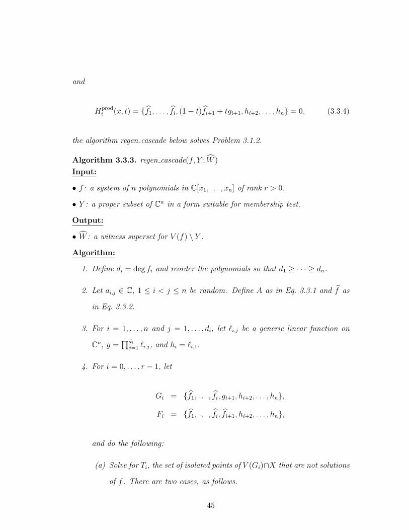
the algorithm regen cascade below solves Problem 3.1.2.
Algorithm 3.3.3. regen cascade(f, Y ; W )
Input:
• f : a system of n polynomials in C[x1, . . . , xn] of rank r > 0.
• Y : a proper subset of Cn in a form suitable for membership test.
Output:
• W : a witness superset for V (f) \ Y .
Algorithm:
1. Define di = deg fi and reorder the polynomials so that d1 ≥ · · · ≥ dn.
2. Let ai,j ∈ C, 1 ≤ i < j ≤ n be random. Define A as in Eq. 3.3.1 and f as
in Eq. 3.3.2.
3. For i = 1, . . . , n and j = 1, . . . , di, let `i,j be a generic linear function on
Cn, g =∏di
j=1 `i,j, and hi = `i,1.
4. For i = 0, . . . , r − 1, let
Gi = {f1, . . . , fi, gi+1, hi+2, . . . , hn},
Fi = {f1, . . . , fi, fi+1, hi+2, . . . , hn},
and do the following:
(a) Solve for Ti, the set of isolated points of V (Gi)∩X that are not solutions
of f . There are two cases, as follows.
45
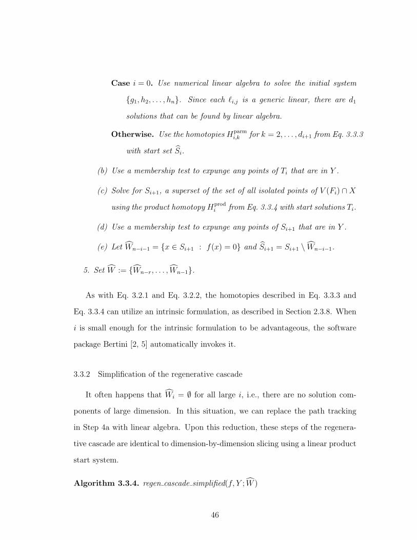
Case i = 0. Use numerical linear algebra to solve the initial system
{g1, h2, . . . , hn}. Since each `i,j is a generic linear, there are d1
solutions that can be found by linear algebra.
Otherwise. Use the homotopies Hparmi,k for k = 2, . . . , di+1 from Eq. 3.3.3
with start set Si.
(b) Use a membership test to expunge any points of Ti that are in Y .
(c) Solve for Si+1, a superset of the set of all isolated points of V (Fi) ∩X
using the product homotopy Hprodi from Eq. 3.3.4 with start solutions Ti.
(d) Use a membership test to expunge any points of Si+1 that are in Y .
(e) Let Wn−i−1 = {x ∈ Si+1 : f(x) = 0} and Si+1 = Si+1 \ Wn−i−1.
5. Set W := {Wn−r, . . . , Wn−1}.
As with Eq. 3.2.1 and Eq. 3.2.2, the homotopies described in Eq. 3.3.3 and
Eq. 3.3.4 can utilize an intrinsic formulation, as described in Section 2.3.8. When
i is small enough for the intrinsic formulation to be advantageous, the software
package Bertini [2, 5] automatically invokes it.
3.3.2 Simplification of the regenerative cascade
It often happens that Wi = ∅ for all large i, i.e., there are no solution com-
ponents of large dimension. In this situation, we can replace the path tracking
in Step 4a with linear algebra. Upon this reduction, these steps of the regenera-
tive cascade are identical to dimension-by-dimension slicing using a linear product
start system.
Algorithm 3.3.4. regen cascade simplified(f, Y ; W )
46
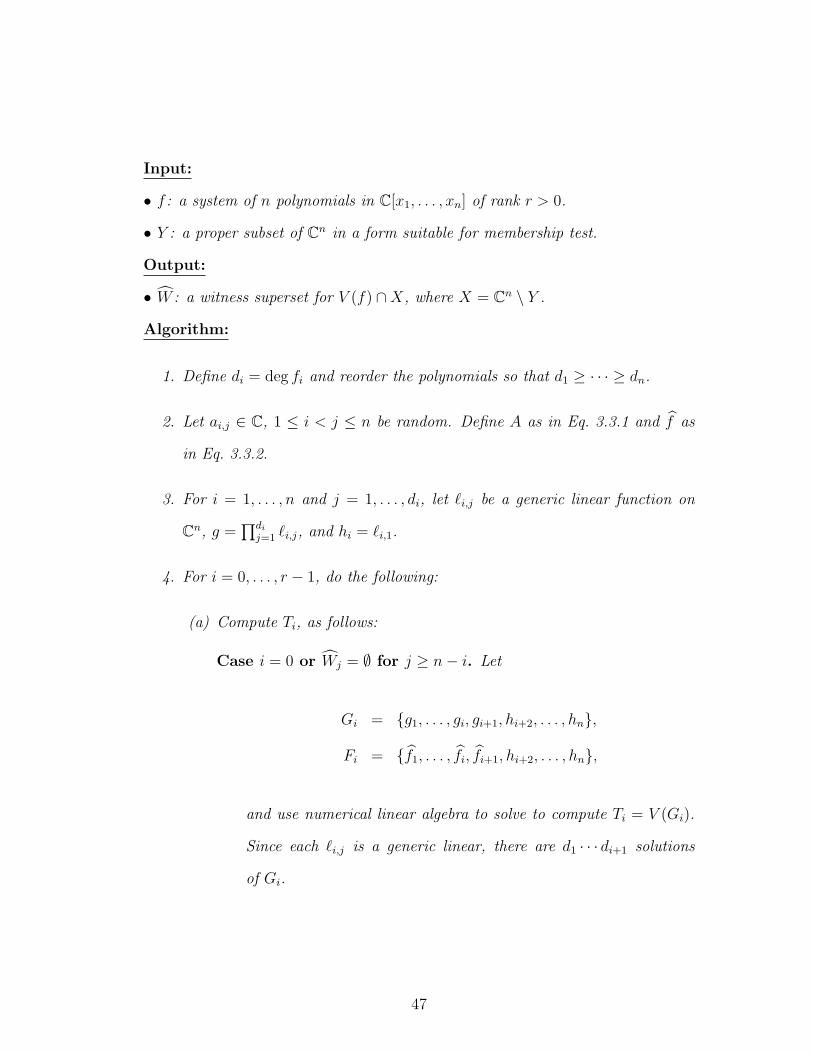
Input:
• f : a system of n polynomials in C[x1, . . . , xn] of rank r > 0.
• Y : a proper subset of Cn in a form suitable for membership test.
Output:
• W : a witness superset for V (f) ∩X, where X = Cn \ Y .
Algorithm:
1. Define di = deg fi and reorder the polynomials so that d1 ≥ · · · ≥ dn.
2. Let ai,j ∈ C, 1 ≤ i < j ≤ n be random. Define A as in Eq. 3.3.1 and f as
in Eq. 3.3.2.
3. For i = 1, . . . , n and j = 1, . . . , di, let `i,j be a generic linear function on
Cn, g =∏di
j=1 `i,j, and hi = `i,1.
4. For i = 0, . . . , r − 1, do the following:
(a) Compute Ti, as follows:
Case i = 0 or Wj = ∅ for j ≥ n− i. Let
Gi = {g1, . . . , gi, gi+1, hi+2, . . . , hn},
Fi = {f1, . . . , fi, fi+1, hi+2, . . . , hn},
and use numerical linear algebra to solve to compute Ti = V (Gi).
Since each `i,j is a generic linear, there are d1 · · · di+1 solutions
of Gi.
47
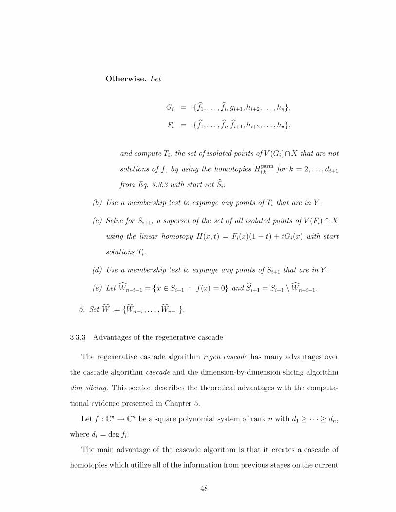
Otherwise. Let
Gi = {f1, . . . , fi, gi+1, hi+2, . . . , hn},
Fi = {f1, . . . , fi, fi+1, hi+2, . . . , hn},
and compute Ti, the set of isolated points of V (Gi)∩X that are not
solutions of f , by using the homotopies Hparmi,k for k = 2, . . . , di+1
from Eq. 3.3.3 with start set Si.
(b) Use a membership test to expunge any points of Ti that are in Y .
(c) Solve for Si+1, a superset of the set of all isolated points of V (Fi) ∩X
using the linear homotopy H(x, t) = Fi(x)(1 − t) + tGi(x) with start
solutions Ti.
(d) Use a membership test to expunge any points of Si+1 that are in Y .
(e) Let Wn−i−1 = {x ∈ Si+1 : f(x) = 0} and Si+1 = Si+1 \ Wn−i−1.
5. Set W := {Wn−r, . . . , Wn−1}.
3.3.3 Advantages of the regenerative cascade
The regenerative cascade algorithm regen cascade has many advantages over
the cascade algorithm cascade and the dimension-by-dimension slicing algorithm
dim slicing. This section describes the theoretical advantages with the computa-
tional evidence presented in Chapter 5.
Let f : Cn → Cn be a square polynomial system of rank n with d1 ≥ · · · ≥ dn,
where di = deg fi.
The main advantage of the cascade algorithm is that it creates a cascade of
homotopies which utilize all of the information from previous stages on the current
48

stage. This creates a witness superset which generally has many fewer junk points
than the dimension-by-dimension slicing algorithm. The two main disadvantages
of this algorithm is that to start the cascade algorithm, the total degree number
of paths, namely d1 · · · dn, need to be tracked, and each stage of the cascade
algorithm tracks using n variables. For large systems, these disadvantages make
the cascade algorithm prohibitively expensive.
The main advantage of the dimension-by-dimension slicing algorithm is the
ability to use intrinsic slicing to reduce the number of tracking variables. The
main disadvantage of this algorithm is that each dimension is handled indepen-
dently, which means that valuable information regarding all larger dimensional
components is not utilized. This generally leads to a witness superset that con-
tains more junk points than the cascade algorithm.
The regenerative cascade algorithm combines the advantages and overcomes
the disadvantages described above for the cascade and dimension-by-dimension
slicing algorithms. First, the regenerative cascade algorithm can utilize intrinsic
slicing to reduce the number of tracking variables. Additionally, this algorithm
creates a sequence of homotopies that utilize all of the information from previous
stages on the current stage by only regenerating the nonsolutions at each stage.
This creates a witness superset that generally has many fewer junk points than
a witness superset created by dimension-by-dimension slicing, and computational
evidence, such as will be shown later in Table 5.6, suggests that the number of junk
points is the same as that created by the cascade algorithm. This is summarized
in the following conjecture.
Conjecture 3.3.5. The algorithms cascade and regen cascade produce witness
supersets that have the same number of junk points for each dimension.
49

CHAPTER 4
LOCAL DIMENSION TEST
For a polynomial system f and a solution x ∈ V (f), the local dimension test
computes the maximum dimension of the varieties V ⊂ V (f) with x ∈ V . This
algorithm is valuable in many circumstances, including
1. determine whether a given solution is isolated (and computing the multi-
plicity if it is);
2. computing the local dimension for a given solution;
3. finding all varieties that contain a given solution;
4. filtering junk points from witness supersets;
5. computing the varieties of V (f) of a prescribed dimension.
Computational evidence presented in Chapter 5 indicates that the efficiency of this
method will have a significant impact on the structure of many of the algorithms
in numerical algebraic geometry, most importantly the numerical irreducible de-
composition. The following sections mostly follow [1].
4.1 Introduction
The following definition describes the local dimension at a solution.
50
Definition 4.1.1 (Local dimension). Let f : CN → Cn be a polynomial system
and x ∈ V (f). The local dimension of x with respect to f , denoted dimx(V (f)),
is
dimx(V (f)) = max{dim(V ) : x ∈ V ⊂ V (f) where V is a variety}.
The algorithms presented below to compute the local dimension at a solution x
with respect to a polynomial system f use the theory of Macaulay [29] and, more
specifically, the numerical approach of Dayton and Zeng [12]. The basic idea in
calculus terms is that the dimensions Tk of the space of Taylor series expansions
of degree at most k of algebraic functions on V (f) at the point x eventually grow
like O(kdimx(V (f))). If dimx(V (f)) = 0, the dimensions Tk steadily grow until they
reach the multiplicity µx of the point x and are constant from that point on. If
dimx(V (f)) > 0, these dimensions steadily grow without bound. If νx is an upper
bound on the multiplicity µx, we have a simple test to check whether x is isolated:
1. Compute the dimensions Tk until the minimum k = k, where
k := min {k ≥ 1 : Tk = Tk−1 or Tk > νx} .
2. Then, x is isolated if and only if Tbk ≤ νx.
One way to compute an upper bound on µx is to count the number of paths which
converge to x for standard homotopies.
If V (f) ⊂ CN is k-dimensional at a point x, then, for 0 ≤ ` ≤ k, a general
linear space L through x of dimension equal to N − k + ` will meet V (f) in an
algebraic subset of dimension ` at x. Using this fact, we turn the above algorithm
for whether a point is isolated into an algorithm for computing the maximum
dimension of the varieties of V (f) containing x.
51

Though the local dimension test in this thesis is the first rigorous numerical
local dimension algorithm that applies to arbitrary polynomial systems, it is not
the first numerical method proposed to compute local dimensions. Using the facts
about slicing V with linear spaces L:
• If V (f) ⊂ CN is k-dimensional at a point x, then a general linear space L
through that point of dimension less than or equal to N − k will meet V (f)
in no other points in a neighborhood of x; and
• given a general linear space L of dimension greater than N − k, L ∩ V (f)
will contain points in a neighborhood of x,
Sommese and Wampler [43, § 3.3] showed that the local dimension dimx(V (f))
could be determined by choosing an appropriate family Lt of linear spaces with
L0 = L and then deciding whether the point x deforms in V ∩ Lt. They did not
present any numerical method to make this decision. In [22], Kuo and Li present
an interesting heuristical method to make this decision. The method works well
for many examples, but it does not seem possible to turn it into a rigorous local-
dimension algorithm for a point on the solution set of polynomial systems. For
instance, since the method is based on the presentation of the system and not
on intrinsic properties of the solution set, it is not likely that any result covering
general systems can be proved. Indeed, as the simple system in Section 5.3 (con-
sisting of two cubic equations in two variables) shows: solution sets with multiple
branches going through a point may lead the method to give false answers.
4.2 Theory behind the algorithms
For a polynomial system f : CN → Cn and isolated solution x ∈ V (f) of
multiplicity µx, there are known methods for computing its multiplicity [6, 12, 55].
52
In particular, these methods compute a sequence {µk}∞k=0 such that µ0 = 1 and
there exists d ≥ 0 such that µk < µk+1 for 0 ≤ k < d and µk = µx for k ≥ d.
The rest of this section focuses on the theory of Macaulay [29], which is used in
the methods of [12, 55], to describe the behavior of the sequence µk at solutions
which may not be isolated.
Following the notation of [12], for j ∈ (Z≥0)N , define j! = j1! · · · jN !, |j| =
j1 + · · ·+ jN and
∂j =1
j!
∂|j|
∂xj11 · · · ∂x
jN
N
.
Define the differential functional ∂j[x] : C[x1, . . . , xN ] → C at x ∈ CN as
∂j[x](p) = (∂jp)(x).
The set of differential functionals at x that vanish on the ideal generated by f
is called the dual space of f at x. The dual space, denoted Dx(f), which can be
written
Dx(f) = {∂ =∑
j∈(Z≥0)N
dj∂j[x] : dj ∈ C, ∂ (pfi) = 0,
∀p ∈ C[x1, . . . , xN ], i = 1, . . . , n}, (4.2.1)
is a C-vector space. The following theorem provides the relationship between the
dimension of the dual space and the multiplicity.
Theorem 4.2.1. Let f be a polynomial system and x ∈ V (f). Then, x is an
isolated solution of multiplicity m if and only if dimC (Dx(f)) = m. In particular,
x is isolated if and only if dimC (Dx(f)) <∞.
Stetter and Thallinger [45, 47] provided an equivalent definition of the dual
53
space as follows. For σ ∈ {1, . . . , N}, let eσ be the σth column of the N × N
identity matrix and define the linear anti-differentiation operator Φσ as
Φσ(∂j[x]) =
∂j−eσ [x] if jσ > 0
0 otherwise.
Then, ∂ ∈ Dx(f) if and only if for each i = 1, . . . , n, ∂(fi) = 0 and, for each
σ = 1, . . . , N , Φσ(∂) ∈ Dx(f).
For each k ≥ 0, define
Dkx(f) =
∂ =∑|j|≤k
dj∂j[x] : ∂ ∈ Dx(f)
.
Clearly, Dkx(f) ⊂ Dk+1
x (f) ⊂ Dx(f). The Stetter and Thallinger formulation
yields the following lemma.
Lemma 4.2.2. Let k ≥ 2. If ∂ ∈ Dkx(f)\Dk−1
x (f), there is a σ ∈ {1, . . . , N} such
that Φσ(∂) ∈ Dk−1x (f)\Dk−2
x (f).
Proof. Write ∂ =∑
|j|≤k dj∂j[x]. By assumption, there is j with |j| = k > 0 and
dbj 6= 0. For σ such that jσ > 0, we have Φσ(∂) ∈ Dk−1x (f)\Dk−2
x (f).
The following theorem summarizes the properties of the sequence {µk}∞k=0
defined by
µk = dimC(Dk
x(f)). (4.2.2)
Theorem 4.2.3. Let f be a polynomial system, x ∈ V (f), and µk as in Eq. 4.2.2.
Then, µ0 = 1 and, for each k ≥ 0, either
1. µk < µk+1, or
54
2. µk = µk+i, for all i ≥ 1, and x is isolated of multiplicity µk.
Proof. Trivially, for 0 = (0, . . . , 0), ∂0[x](pfi) = p(x)fi(x) = 0 for all p ∈ C[x1, . . . ,
xN ] since x ∈ V (f). That is, D0x(f) = {d ∂0 : d ∈ C} is a C-vector space of
dimension 1. Now, for k ≥ 0, we have µk ≤ µk+1 by definition. Assume that
µk ≮ µk+1, i.e., µk = µk+1. In particular, Dk+1x (f) = Dk
x(f). If µk+2 > µk+1,
then there is ∂ ∈ Dk+2x (f)\Dk+1
x (f). By Lemma 4.2.2, there exists σ such Φσ(∂) ∈
Dk+1x (f)\Dk
x(f) = ∅, yielding a contradiction. That is, µk+2 = µk+1 = µk and, by
induction, µk+i = µk for all i ≥ 1. Theorem 2 of [12] yields that x is isolated of
multiplicity µk.
4.3 Algorithms
With the theoretical foundation presented in Section 4.2, we present the fol-
lowing five algorithms:
1. determine whether a given solution is isolated (and computing the multi-
plicity if it is);
2. compute the local dimension for a given solution;
3. find all varieties that contain a given solution;
4. filter junk points efficiently;
5. compute the varieties of V (f) of a prescribed dimension.
These algorithms depend upon two operations, namely multiplicity and find bound.
The operation multiplicity(f, x, k) returns µk defined by Eq. 4.2.2, in which the
methods of [12, 55] can be used. The operation find bound(f, x) returns a bound
on the multiplicity of x as a solution of f . An upper bound can be determined by
55

using homotopy continuation and simply counting the number of solution paths
converging to x. This upper bound along with Thm. 4.2.3 provides the stopping
criterion if x is not isolated.
The first algorithm, called is isolated, determines if x is isolated. It computes
µk until either µk = µk+1 (isolated of multiplicity µk) or µk is larger than the
bound provided by find bound (not isolated).
Algorithm 4.3.1. is isolated(f, x, B; is isolatedx, µx)
Input:
• f : a system of n polynomials in C[x1, . . . , xN ].
• x: a point on V (f) ⊂ CN .
• B: an upper bound on the multiplicity of x if it is isolated.
Output:
• is isolatedx: True, if x is isolated, otherwise False.
• µx: the multiplicity if x is isolated.
Algorithm:
1. Initialize k := 1, µ0 := 1, and µ1 := multiplicity(f, x, 1).
2. While µk−1 < µk ≤ B, do the following:
(a) Increment k := k + 1.
(b) µk := multiplicity(f, x, k).
3. If µk ≤ B, then is isolatedx := True and µx := µk, otherwise is isolatedx :=
False.
The second algorithm, called local dimension, uses is isolated along with linear
slicing to determine the local dimension.
56
Algorithm 4.3.2. local dimension(f, x; dimx)
Input:
• f : a system of n polynomials in C[x1, . . . , xN ].
• x: a point on V (f) ⊂ CN .
Output:
• dimx: the local dimension at x.
Algorithm:
1. Choose L1, . . . , LN random linear forms through x on CN , and set k := −1.
2. Initialize is isolatedk := False.
3. While is isolatedk = False, do the following:
(a) Increment k := k + 1.
(b) Bk := find bound({f, L1, . . . , Lk}, x).
(c) (is isolatedk, µk) := is isolated({f, L1, . . . , Lk}, x, Bk).
4. Set dimx := k.
The third algorithm, called irreducible components, uses an irreducible decom-
position of V (f) and membership, as described in Sections 2.2 and 2.4.2, respec-
tively, to decide which varieties the given solution lies on.
Algorithm 4.3.3. irreducible components(f,W, x; J)
Input:
• f : a system of n polynomials in C[x1, . . . , xN ].
• W : an irreducible decomposition of f .
• x: a point on V (f) ⊂ CN .
Output:
57
• J : a set of pairs of numbers, each representing the dimension and component
number of an irreducible component of which x is a member.
Algorithm:
1. Initialize J = {}.
2. Compute dimx := local dimension(f, x).
3. For j := 0, . . . , dimx, do the following:
(a) Set m := number of irreducible components of dimension j in Wj.
(b) For k := 1, . . . ,m, if membership(x,Wjk), J := J ∪ {(j, k)}.
The fourth algorithm, called junk removal ldt, uses is isolated to remove the
junk points from a witness superset. The witness superset algorithms cascade,
dim slicing, and regen cascade provide an upper bound on the multiplicity, which
is the number of paths that limit to the solution.
Algorithm 4.3.4. junk removal ldt(W ;W )
Input:
• W : a witness superset for an algebraic set X.
Output:
• W : a witness set for X.
Algorithm:
1. Let f be the polynomial system associated with W and let W = {W0, . . . , Wd}.
2. Initialize W0, . . . ,Wd−1 := ∅ and Wd := Wd.
3. For k := d− 1, . . . , 0, do the following:
(a) Let Lk be the system of linear functions associated with Wk.
58

(b) For each y ∈ Wk, do the following:
i. Let B be the bound on the multiplicity of y, if y is an isolated
solution of {f, Lk}.
ii. If is isolated({f, Lk}, y, B), append y to Wk.
4. Set W := {W0, . . . ,Wd}.
The final algorithm, called decompose dim k, uses junk removal ldt to compute
the varieties of V (f) of a given dimension. When using junk removal mem (Algo-
rithm 2.4.11), a witness set is needed for all higher dimensions in order to identify
the junk points for a given dimension, which is not the case when using the local
dimension test.
Algorithm 4.3.5. decompose dim k(f, k;W )
Input:
• f : a system of n polynomials in C[x1, . . . , xN ].
Output:
• W : witness set for the dimension k varieties of V (f) decomposed as in Eq. 2.2.1.
Algorithm:
1. [W ] := dim slicing k(f, k).
2. [Wp] := junk removal ldt(f, W ).
3. [W ] := irreducible decomp(f,Wp).
59

CHAPTER 5
COMPUTATIONAL RESULTS
The following sections provide computational evidence of the advantages of
using regeneration, regenerative cascade and the local dimension test. The serial
computations were run on an Opteron 250 processor with 64-bit Linux and the
parallel computations were run on a cluster consisting of a manager that uses
one core of a Xeon 5410 processor and an additional 8 computing nodes each
containing two Xeon 5410 processors running 64-bit Linux. The version 1.1.1.
of the Bertini software package [2, 5] was used, with this version utilizing the
multiplicity method of [12] in the local dimension computations.
Section 5.1 presents an example that compares regeneration and the diagonal
homotopy approach of [42] for computing the isolated solutions of a polynomial
system arising in kinematics.
Section 5.2 compares regeneration with the polyhedral homotopy method [20,
27, 50], currently considered the most efficient non-incremental way of solving
sparse polynomial systems, on a collection of sparse polynomial systems aris-
ing from the discretization of nonlinear partial differential equations. Polyhedral
homotopies are implemented in PHCpack [48] and HOM4PS-2.0 [25] with the
computations using PHCpack v2.3.39 and HOM4PS-2.0.15.
Section 5.3 presents an example to illustrate potential difficulties arising in the
heuristic local dimension approach of [22].
60
Section 5.4 presents a collection of examples to demonstrate the application of
the regenerative cascade and the local dimension test for computing the numerical
irreducible decomposition.
Finally, Section 5.5 presents computational results for the decomposition of
permanental ideals.
5.1 A comparison of the equation-by-equation methods
To compare the equation-by-equation approaches using the diagonal homo-
topy [42] and regeneration, consider a polynomial system arising from the inverse
kinematics problem of general six-revolute, serial-link robots described in [44, 53].
The polynomial system, available at [2], consists of 2 linear and 10 quadratic
polynomials in 12 variables with total degree 1, 024. The system was constructed
using random parameter values and is known to have 16 nonsingular finite isolated
solutions.
As mentioned in Section 3.2.4, the ordering of the quadratic polynomials that
minimizes the total number of paths that need to be tracked is suggested by the
construction of the polynomials in the system. In this problem, the 12 variables
correspond to the entries of 4 vectors in C3. Four of the quadratics correspond to
normalizing each of these vectors to unit length. The other six quadratics provide
conditions on the interaction between two or more vectors. This suggests that the
four normalizing quadratics should be placed last. We shall call this optimal setup
“order A” and, for comparison, consider another ordering, called “order B”, that
places the four normalizing quadratics ahead of the other six quadratics. The total
number of paths tracked by regeneration was 628 and 928 and the total number
of slices moved was 313 and 463 for “order A” and “order B”, respectively.
61
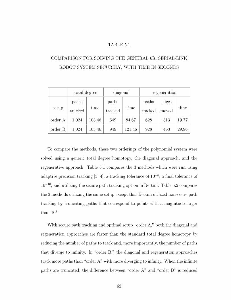
TABLE 5.1
COMPARISON FOR SOLVING THE GENERAL 6R, SERIAL-LINK
ROBOT SYSTEM SECURELY, WITH TIME IN SECONDS
total degree diagonal regeneration
paths paths paths slices
setuptracked
timetracked
timetracked moved
time
order A 1,024 103.46 649 84.67 628 313 19.77
order B 1,024 103.46 949 121.46 928 463 29.96
To compare the methods, these two orderings of the polynomial system were
solved using a generic total degree homotopy, the diagonal approach, and the
regenerative approach. Table 5.1 compares the 3 methods which were run using
adaptive precision tracking [3, 4], a tracking tolerance of 10−6, a final tolerance of
10−10, and utilizing the secure path tracking option in Bertini. Table 5.2 compares
the 3 methods utilizing the same setup except that Bertini utilized nonsecure path
tracking by truncating paths that correspond to points with a magnitude larger
than 108.
With secure path tracking and optimal setup “order A,” both the diagonal and
regeneration approaches are faster than the standard total degree homotopy by
reducing the number of paths to track and, more importantly, the number of paths
that diverge to infinity. In “order B,” the diagonal and regeneration approaches
track more paths than “order A” with more diverging to infinity. When the infinite
paths are truncated, the difference between “order A” and “order B” is reduced
62
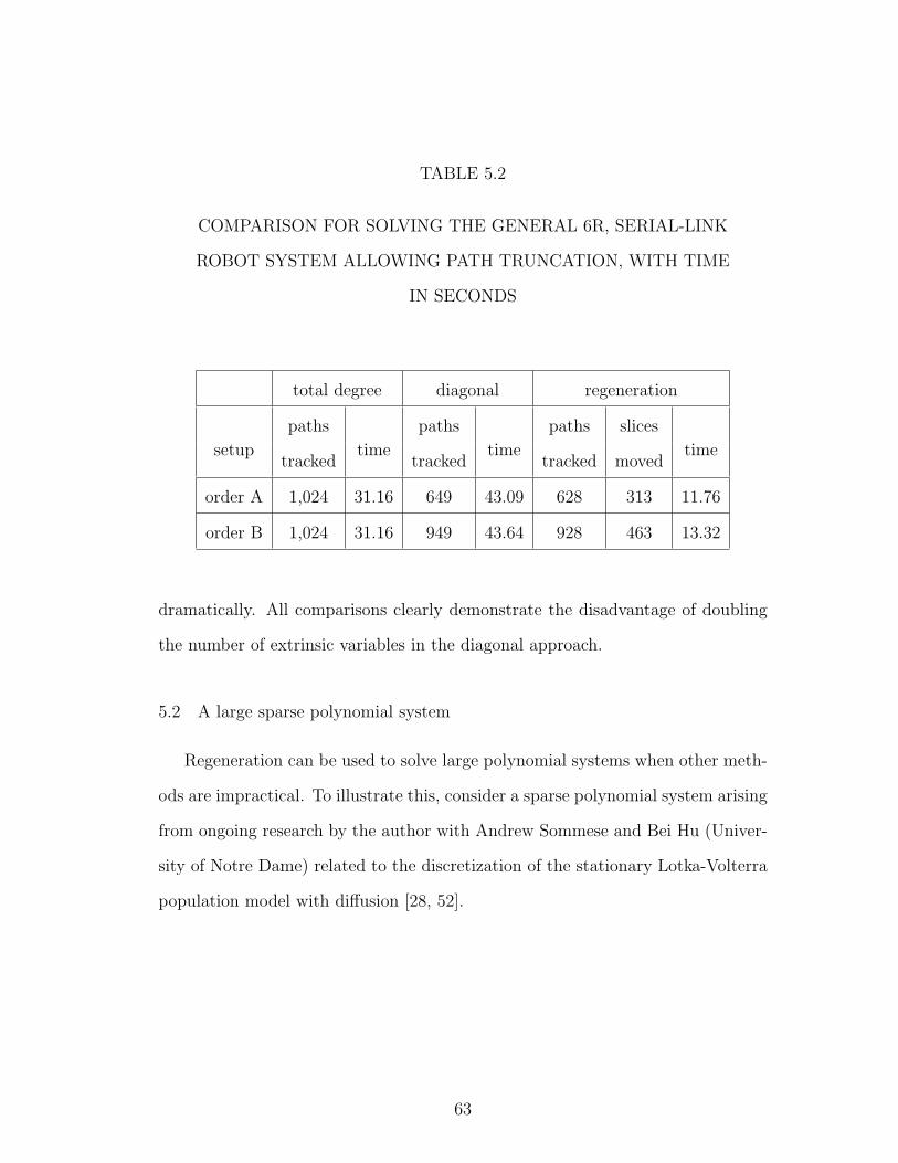
TABLE 5.2
COMPARISON FOR SOLVING THE GENERAL 6R, SERIAL-LINK
ROBOT SYSTEM ALLOWING PATH TRUNCATION, WITH TIME
IN SECONDS
total degree diagonal regeneration
paths paths paths slices
setuptracked
timetracked
timetracked moved
time
order A 1,024 31.16 649 43.09 628 313 11.76
order B 1,024 31.16 949 43.64 928 463 13.32
dramatically. All comparisons clearly demonstrate the disadvantage of doubling
the number of extrinsic variables in the diagonal approach.
5.2 A large sparse polynomial system
Regeneration can be used to solve large polynomial systems when other meth-
ods are impractical. To illustrate this, consider a sparse polynomial system arising
from ongoing research by the author with Andrew Sommese and Bei Hu (Univer-
sity of Notre Dame) related to the discretization of the stationary Lotka-Volterra
population model with diffusion [28, 52].
63
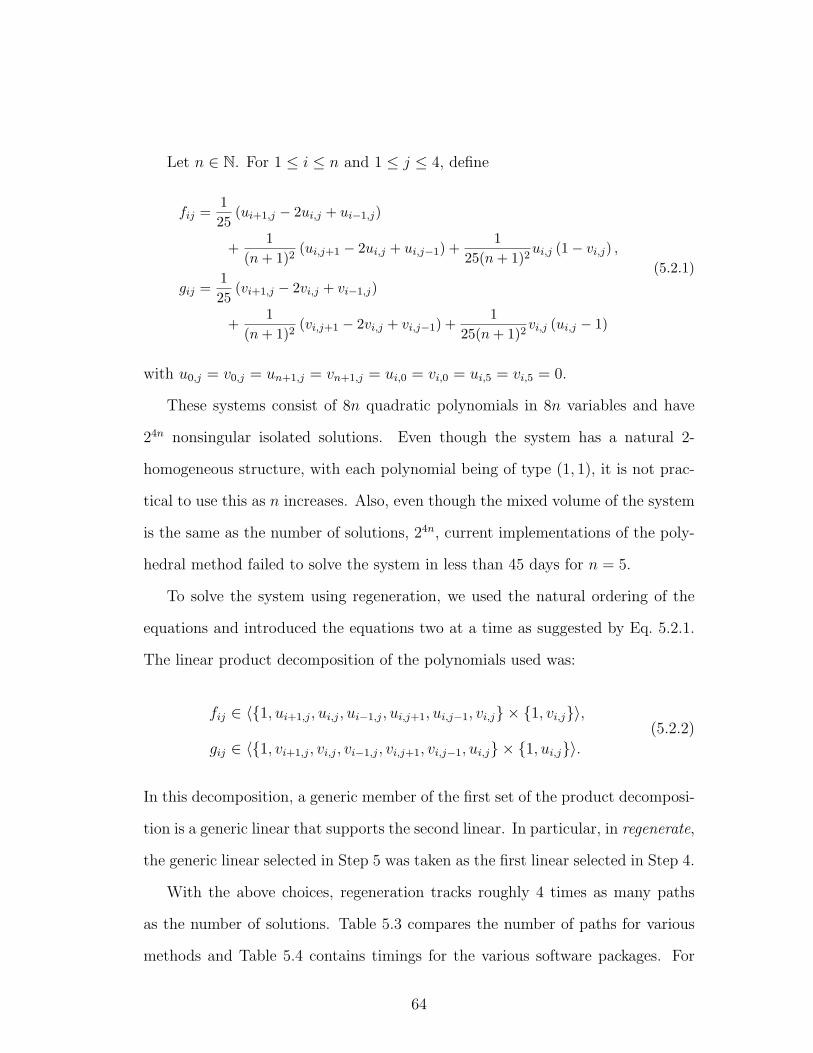
Let n ∈ N. For 1 ≤ i ≤ n and 1 ≤ j ≤ 4, define
fij =125
(ui+1,j − 2ui,j + ui−1,j)
+1
(n + 1)2(ui,j+1 − 2ui,j + ui,j−1) +
125(n + 1)2
ui,j (1− vi,j) ,
gij =125
(vi+1,j − 2vi,j + vi−1,j)
+1
(n + 1)2(vi,j+1 − 2vi,j + vi,j−1) +
125(n + 1)2
vi,j (ui,j − 1)
(5.2.1)
with u0,j = v0,j = un+1,j = vn+1,j = ui,0 = vi,0 = ui,5 = vi,5 = 0.
These systems consist of 8n quadratic polynomials in 8n variables and have
24n nonsingular isolated solutions. Even though the system has a natural 2-
homogeneous structure, with each polynomial being of type (1, 1), it is not prac-
tical to use this as n increases. Also, even though the mixed volume of the system
is the same as the number of solutions, 24n, current implementations of the poly-
hedral method failed to solve the system in less than 45 days for n = 5.
To solve the system using regeneration, we used the natural ordering of the
equations and introduced the equations two at a time as suggested by Eq. 5.2.1.
The linear product decomposition of the polynomials used was:
fij ∈ 〈{1, ui+1,j, ui,j, ui−1,j, ui,j+1, ui,j−1, vi,j} × {1, vi,j}〉,
gij ∈ 〈{1, vi+1,j, vi,j, vi−1,j, vi,j+1, vi,j−1, ui,j} × {1, ui,j}〉.(5.2.2)
In this decomposition, a generic member of the first set of the product decomposi-
tion is a generic linear that supports the second linear. In particular, in regenerate,
the generic linear selected in Step 5 was taken as the first linear selected in Step 4.
With the above choices, regeneration tracks roughly 4 times as many paths
as the number of solutions. Table 5.3 compares the number of paths for various
methods and Table 5.4 contains timings for the various software packages. For
64
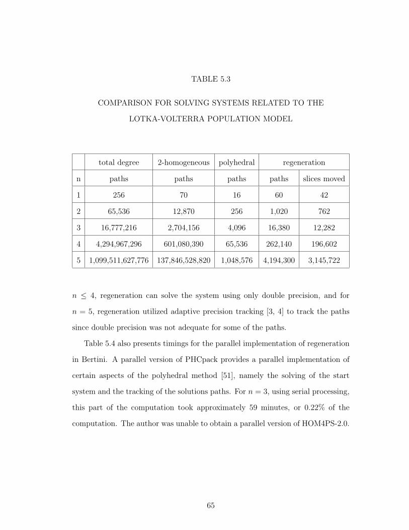
TABLE 5.3
COMPARISON FOR SOLVING SYSTEMS RELATED TO THE
LOTKA-VOLTERRA POPULATION MODEL
total degree 2-homogeneous polyhedral regeneration
n paths paths paths paths slices moved
1 256 70 16 60 42
2 65,536 12,870 256 1,020 762
3 16,777,216 2,704,156 4,096 16,380 12,282
4 4,294,967,296 601,080,390 65,536 262,140 196,602
5 1,099,511,627,776 137,846,528,820 1,048,576 4,194,300 3,145,722
n ≤ 4, regeneration can solve the system using only double precision, and for
n = 5, regeneration utilized adaptive precision tracking [3, 4] to track the paths
since double precision was not adequate for some of the paths.
Table 5.4 also presents timings for the parallel implementation of regeneration
in Bertini. A parallel version of PHCpack provides a parallel implementation of
certain aspects of the polyhedral method [51], namely the solving of the start
system and the tracking of the solutions paths. For n = 3, using serial processing,
this part of the computation took approximately 59 minutes, or 0.22% of the
computation. The author was unable to obtain a parallel version of HOM4PS-2.0.
65

TABLE 5.4
COMPARISON OF POLYHEDRAL METHOD AND
REGENERATION FOR SOLVING SYSTEMS RELATED TO THE
LOTKA-VOLTERRA POPULATION MODEL
PHC HOM4PS-2.0 Bertini
n polyhedral polyhedral regeneration parallel regeneration
1 0.6s 0.1s 0.3s
2 4m57s 7.3s 15.6s
3 18d10h18m56s 9m32s 9m43s
4 - 3d8h28m30s 5h22m15s 7m32s
5 - - 6d16h27m3s 3h41m24s
66

−1 −0.8 −0.6 −0.4 −0.2 0 0.2 0.4 0.6 0.8 1−1
−0.8
−0.6
−0.4
−0.2
0
0.2
0.4
0.6
0.8
1
Figure 5.1. Rhodonea curves S7 and S5.
5.3 A local dimension example
Rhodonea curves, such as those displayed in Figure 5.1, are defined by polar
equations of the form r = sin(kθ). Denote the curve defined by the polar equation
r = sin(kθ) by Sk and let Sk denote the curve obtained by applying a random
rotation about the origin to Sk. For k even, Sk has 2k “petals” and for k odd,
Sk has k “petals.” For pairs of odd integers m and n, the origin is an isolated
solution of the pair of equations defining the curves Sm and Sn. Due to the random
rotation about the origin, the petals of Sm and Sn do not share a common tangent
direction at the origin. As a result, the multiplicity at the origin is mn.
The Rhodonea curve S1 is the solution set of the polynomial g(x, y) = x2 +
y2 − y. That is, S1 is the circle of radius 12
centered at(0, 1
2
). For a 2× 2 random
67

real orthogonal matrix A, define (x, y) by
x
y
= A
x
y
.The solution set S1 of g(x, y) = g(x, y) is a rotation of S1 about the origin. The
set S1 ∩ S1 is the solution set of the system g(x, y) = g(x, y) = 0 which consists of
the 2 intersection points of the corresponding two circles, namely the origin and
the point (x, y) away from the origin.
Let f1(x, y) = xg(x, y) and f2(x, y) = xg(x, y). The algebraic set V (f1, f2) has
2 irreducible components: the isolated point p = (x, y) and the line L = {x = 0}.
It can be shown that the origin is an embedded point of the line L. Bertini used
a total degree homotopy and found 2 paths that lead to the origin. Since the
Jacobian of the system is the zero matrix at the origin, the multiplicity must
be at least 3 in order for the origin to be an isolated solution. The algorithm
is isolated identified that the origin is not isolated in 0.005 seconds. The full
numerical irreducible decomposition was completed by Bertini in 0.11 seconds.
The Matlab module described in [22] used a polyhedral homotopy which also
had 2 paths leading to the origin. However, it was unable to identify that the
origin lies on a one-dimensional component. The module did correctly identify
(x, y) as isolated and that another point of the form (0, y′) (with y′ 6= 0) was a
point lying on a one-dimensional component.
5.4 A collection of high-dimensional examples
Computing a numerical irreducible decomposition for a given polynomial sys-
tem is a fundamental algorithm in numerical algebraic geometry. For systems
68
with components in many different dimensions, the dimension-by-dimension slic-
ing algorithm dim slicing generally produces a witness superset that contains more
junk points than the cascade algorithm cascade and the regenerative cascade al-
gorithm regen cascade. No matter which algorithm is used to construct a witness
superset, filtering out the junk points using the membership test junk removal
algorithm junk removal mem can result in a bottleneck. By using the local di-
mension test junk removal algorithm junk removal ldt, the filtering of junk points
is very efficient.
Consider the homogeneous polynomial system Fk,m,n constructed by taking the
determinants of the k × k adjacent minors of an m× n matrix of indeterminants
[13, 18, 19, 46]. In [13], it was shown that V (F2,2,n) has codimension n−1, degree
2n−1, and decomposes into f(n) varieties, where f(n) = f(n− 1)+ f(n− 2) is the
nth Fibonacci number with starting values f(0) = 0 and f(1) = 1. This result was
generalized to Fm,m,n in [19], namely V (Fm,m,n) has codimension n−m+1, degree
mn−m+1, and decomposes into fm(n) varieties, where fm(n) = fm(n − 1) + · · · +
fm(n−m) with starting values fm(0) = · · · = fm(m− 2) = 0 and fm(m− 1) = 1.
The system F2,m,n was studied in both [18] and [19]. A combinatorial descrip-
tion for the generators of the varieties in V (F2,m,n) was presented in [19]. In [18],
it was shown that V (F2,3,n) consists of φ(n) varieties, where φ(n) = φ(n − 1) +
φ(n − 2) +∑n−5
j=0 φ(j) with starting values φ(0) = φ(1) = 1, φ(2) = 2, φ(3) = 3,
and φ(4) = 6. Table 5.5 summarizes the total number of varieties for V (F2,3,n),
3 ≤ n ≤ 9, as well as list the codimension of the varieties.
To compare the algorithms, we computed the numerical irreducible decompo-
sition for V (F2,3,n) with 3 ≤ n ≤ 9. Table 5.6 compares the total number of paths
that are tracked and the number of junk points for the three witness superset
69
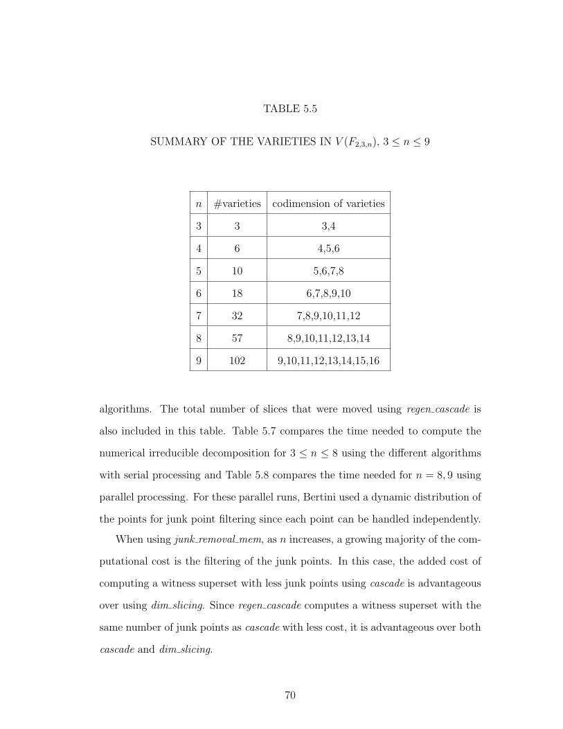
TABLE 5.5
SUMMARY OF THE VARIETIES IN V (F2,3,n), 3 ≤ n ≤ 9
n #varieties codimension of varieties
3 3 3,4
4 6 4,5,6
5 10 5,6,7,8
6 18 6,7,8,9,10
7 32 7,8,9,10,11,12
8 57 8,9,10,11,12,13,14
9 102 9,10,11,12,13,14,15,16
algorithms. The total number of slices that were moved using regen cascade is
also included in this table. Table 5.7 compares the time needed to compute the
numerical irreducible decomposition for 3 ≤ n ≤ 8 using the different algorithms
with serial processing and Table 5.8 compares the time needed for n = 8, 9 using
parallel processing. For these parallel runs, Bertini used a dynamic distribution of
the points for junk point filtering since each point can be handled independently.
When using junk removal mem, as n increases, a growing majority of the com-
putational cost is the filtering of the junk points. In this case, the added cost of
computing a witness superset with less junk points using cascade is advantageous
over using dim slicing. Since regen cascade computes a witness superset with the
same number of junk points as cascade with less cost, it is advantageous over both
cascade and dim slicing.
70
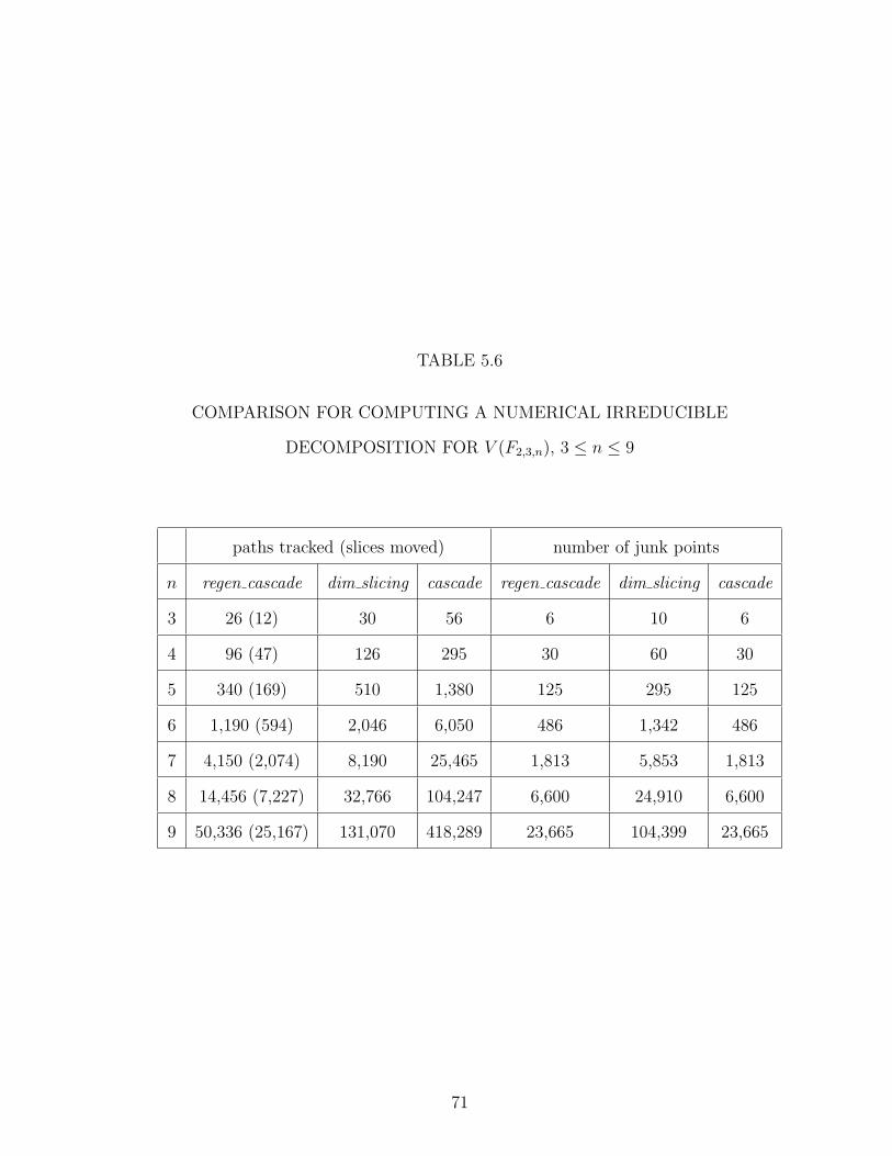
TABLE 5.6
COMPARISON FOR COMPUTING A NUMERICAL IRREDUCIBLE
DECOMPOSITION FOR V (F2,3,n), 3 ≤ n ≤ 9
paths tracked (slices moved) number of junk points
n regen cascade dim slicing cascade regen cascade dim slicing cascade
3 26 (12) 30 56 6 10 6
4 96 (47) 126 295 30 60 30
5 340 (169) 510 1,380 125 295 125
6 1,190 (594) 2,046 6,050 486 1,342 486
7 4,150 (2,074) 8,190 25,465 1,813 5,853 1,813
8 14,456 (7,227) 32,766 104,247 6,600 24,910 6,600
9 50,336 (25,167) 131,070 418,289 23,665 104,399 23,665
71
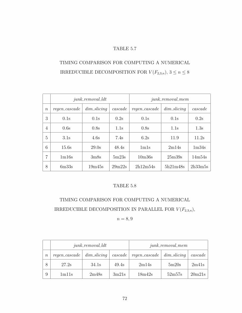
TABLE 5.7
TIMING COMPARISON FOR COMPUTING A NUMERICAL
IRREDUCIBLE DECOMPOSITION FOR V (F2,3,n), 3 ≤ n ≤ 8
junk removal ldt junk removal mem
n regen cascade dim slicing cascade regen cascade dim slicing cascade
3 0.1s 0.1s 0.2s 0.1s 0.1s 0.2s
4 0.6s 0.8s 1.1s 0.8s 1.1s 1.3s
5 3.1s 4.6s 7.4s 6.2s 11.9 11.2s
6 15.6s 29.0s 48.4s 1m1s 2m14s 1m34s
7 1m16s 3m8s 5m23s 10m36s 25m39s 14m54s
8 6m33s 19m45s 29m22s 2h12m54s 5h21m48s 2h33m5s
TABLE 5.8
TIMING COMPARISON FOR COMPUTING A NUMERICAL
IRREDUCIBLE DECOMPOSITION IN PARALLEL FOR V (F2,3,n),
n = 8, 9
junk removal ldt junk removal mem
n regen cascade dim slicing cascade regen cascade dim slicing cascade
8 27.2s 34.1s 49.4s 2m14s 5m20s 2m41s
9 1m11s 2m48s 3m21s 18m42s 52m57s 20m21s
72

When using junk removal ldt, as n increases, a growing majority of the com-
putational cost is the computation of a witness superset. In this case, the reduced
cost of computing a witness superset using dim slicing is advantageous over using
cascade. Since regen cascade computes a witness superset that is computationally
cheaper than dim slicing, it is advantageous over both dim slicing and cascade.
It should be noted that since, for each codimension i, the degree of the algebraic
set consisting of the i-codimensional varieties is considerably smaller than the
total degree of the polynomial system R(F2,3,n, i), the computational cost of using
algorithm irreducible decomp to decompose the witness set into irreducible witness
sets is small compared to the cost of computing the witness set. For example,
using serial processing with n = 8, it took about 57 seconds to decompose the
witness set. For comparison, with junk removal ldt, it took about 336 seconds
using regen cascade, 1, 128 seconds using dim slicing, and 1, 705 seconds using
cascade to compute the witness set.
5.5 Computing the numerical irreducible decomposition for permanental ideals
The system Fk,m,n of Section 5.4 was constructed by taking the determinant of
the k×k adjacent minors of an m×n matrix of indeterminants. Related to Fk,m,n,
consider the homogeneous system Pk,m,n constructed by taking the permanent of
the k × k adjacent minors of an m× n matrix of indeterminants. Previous work,
e.g., [21, 23, 34], has focused on proving primary decomposition results for P2,m,n
and P3,m,n.
The system Pm,m,n consists of n −m + 1 homogeneous polynomials of degree
m in mn variables. For 2 ≤ m ≤ 5 and various values of n, we used Bertini to
compute the numerical irreducible decomposition of Pm,m,n. Tables 5.9, 5.10, 5.11,
73

and 5.12 summarize the results of these computations. Based on these results, we
formulate the following conjecture.
Conjecture 5.5.1. The algebraic set V (Pm,m,n) has codimension n−m+1, degree
mn−m+1, and decomposes into ψm(n) varieties, where
ψm(n) = ψm(n− 1) + ψm(n−m)
with starting values ψm(0) = · · · = ψm(m− 2) = 0 and ψm(m− 1) = 1.
74
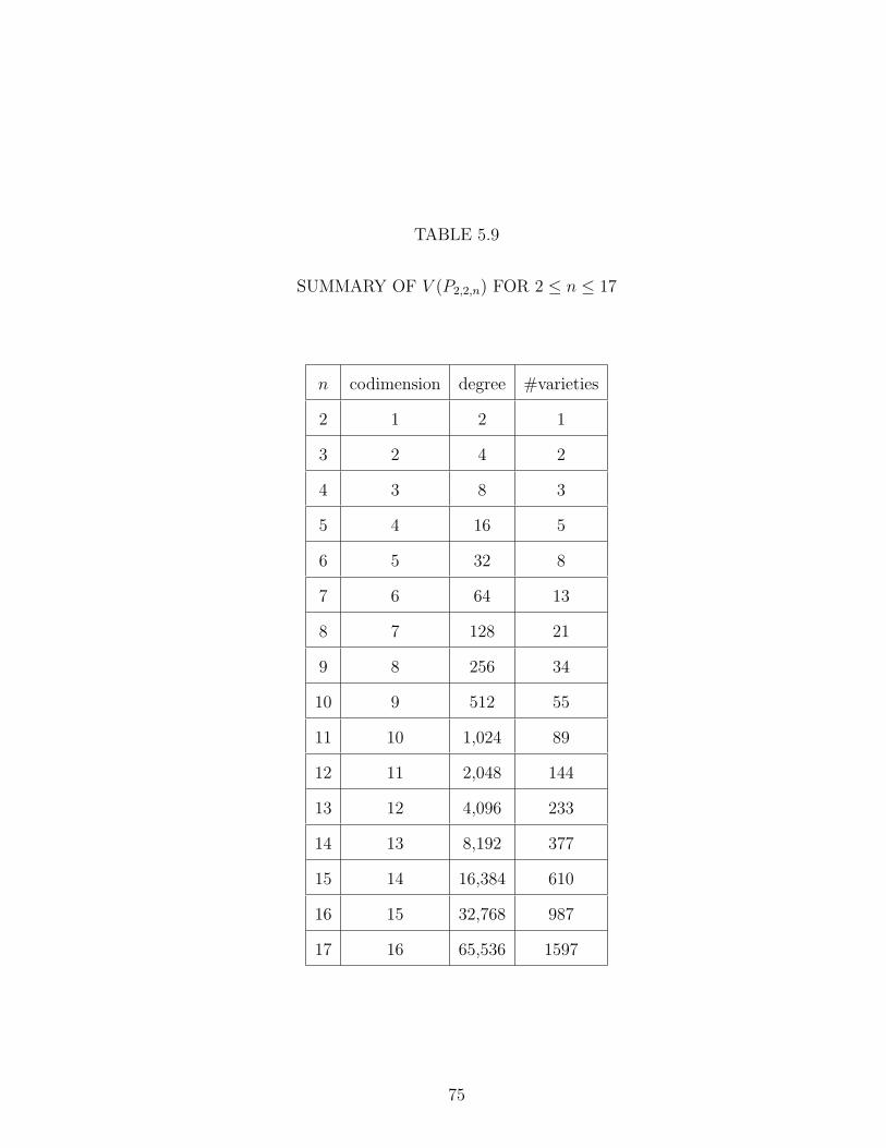
TABLE 5.9
SUMMARY OF V (P2,2,n) FOR 2 ≤ n ≤ 17
n codimension degree #varieties
2 1 2 1
3 2 4 2
4 3 8 3
5 4 16 5
6 5 32 8
7 6 64 13
8 7 128 21
9 8 256 34
10 9 512 55
11 10 1,024 89
12 11 2,048 144
13 12 4,096 233
14 13 8,192 377
15 14 16,384 610
16 15 32,768 987
17 16 65,536 1597
75
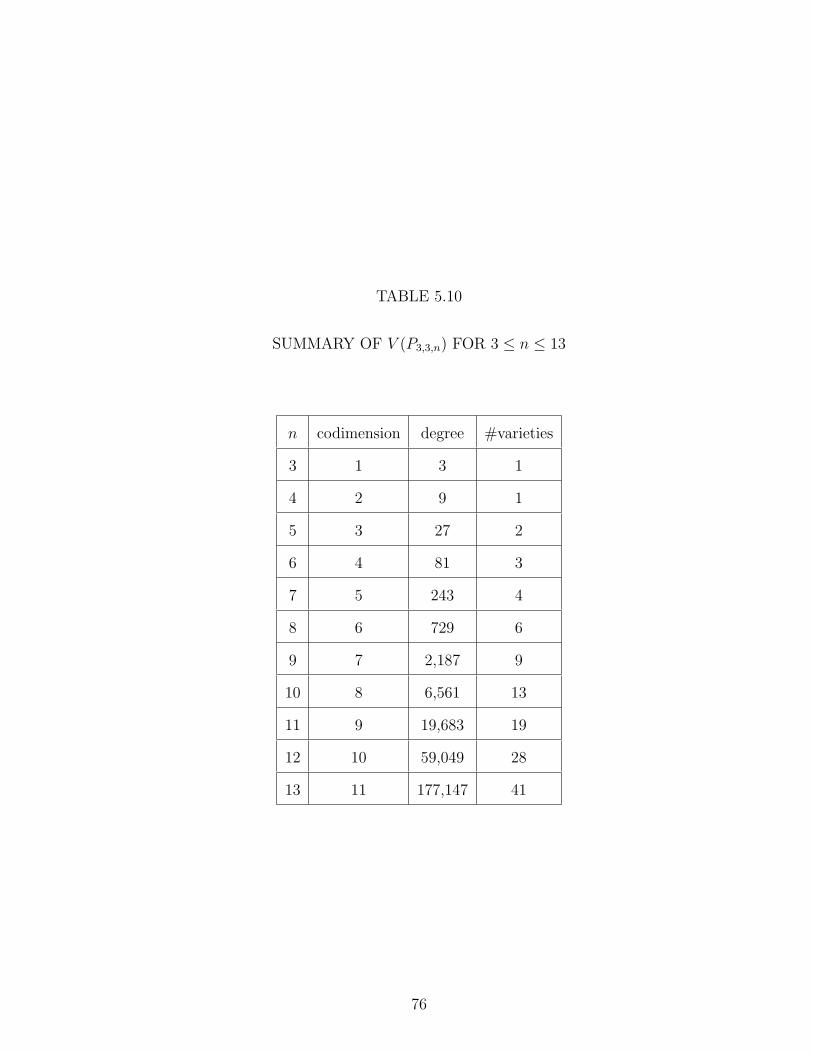
TABLE 5.10
SUMMARY OF V (P3,3,n) FOR 3 ≤ n ≤ 13
n codimension degree #varieties
3 1 3 1
4 2 9 1
5 3 27 2
6 4 81 3
7 5 243 4
8 6 729 6
9 7 2,187 9
10 8 6,561 13
11 9 19,683 19
12 10 59,049 28
13 11 177,147 41
76

TABLE 5.11
SUMMARY OF V (P4,4,n) FOR 4 ≤ n ≤ 12
n codimension degree #varieties
4 1 4 1
5 2 16 1
6 3 64 1
7 4 256 2
8 5 1,024 3
9 6 4,096 4
10 7 16,384 5
11 8 65,536 7
12 9 262,144 10
77

TABLE 5.12
SUMMARY OF V (P5,5,n) FOR 5 ≤ n ≤ 12
n codimension degree #varieties
5 1 5 1
6 2 25 1
7 3 125 1
8 4 625 1
9 5 3,125 2
10 6 15,625 3
11 7 78,125 4
12 8 390,625 5
78
REFERENCES
1. D.J. Bates, J.D. Hauenstein, C. Peterson, and A.J. Sommese. A local dimen-sion test for numerically approximated points on algebraic sets. Preprint, 2009.
2. D.J. Bates, J.D. Hauenstein, A.J. Sommese, and C.W. Wampler.Bertini: Software for numerical algebraic geometry. Available atwww.nd.edu/∼sommese/bertini.
3. D.J. Bates, J.D. Hauenstein, A.J. Sommese, and C.W. Wampler. Adaptivemultiprecision path tracking. SIAM J. Numer. Anal., 46(2):722–746, 2008.
4. D.J. Bates, J.D. Hauenstein, A.J. Sommese, and C.W. Wampler. Stepsizecontrol for adaptive multiprecision path tracking. To appear in Interactionsof Classical and Numerical Algebraic Geometry, D. Bates, G. Besana, S. DiRocco, and C. Wampler (eds.), Contemporary Mathematics, 2009.
5. D.J. Bates, J.D. Hauenstein, A.J. Sommese, and C.W. Wampler, II. Softwarefor numerical algebraic geometry: a paradigm and progress towards its imple-mentation. In Software for algebraic geometry, volume 148 of IMA Vol. Math.Appl., pages 1–14. Springer, New York, 2008.
6. D.J. Bates, C. Peterson, and A.J. Sommese. A numerical-symbolic algorithmfor computing the multiplicity of a component of an algebraic set. J. Com-plexity, 22(4):475–489, 2006.
7. B. Buchberger. Ein Algorithmus zum Auffinden der Basiselmente des Restk-lassenrings nach einem nulldimensionalen Polynomideal. PhD thesis, Univer-sity of Innsbruck, Innsbruck, Austria, 1965.
8. D. Cox, J. Little, and D. O’Shea. Ideals, varieties, and algorithms: An in-troduction to computational algebraic geometry and commutative algebra. Un-dergraduate Texts in Mathematics. Springer-Verlag, New York, second edi-tion, 1997.
9. D. Cox, J. Little, and D. O’Shea. Using algebraic geometry, volume 185 ofGraduate Texts in Mathematics. Springer-Verlag, New York, 1998.
79

10. D.F. Davidenko. On a new method of numerical solution of systems of non-linear equations. Doklady Akad. Nauk SSSR (N.S.), 88:601–602, 1953.
11. D.F. Davidenko. On approximate solution of systems of nonlinear equations.Ukrain. Mat. Zurnal, 5:196–206, 1953.
12. B.H. Dayton and Z. Zeng. Computing the multiplicity structure in solvingpolynomial systems. In ISSAC’05, pages 116–123 (electronic). ACM, NewYork, 2005.
13. P. Diaconis, D. Eisenbud, and B. Sturmfels. Lattice walks and primary decom-position. In Mathematical essays in honor of Gian-Carlo Rota (Cambridge,MA, 1996), volume 161 of Progr. Math., pages 173–193. Birkhauser Boston,Boston, MA, 1998.
14. W. Fulton. Algebraic curves. An introduction to algebraic geometry. W. A.Benjamin, Inc., New York-Amsterdam, 1969. Notes written with the collab-oration of Richard Weiss, Mathematics Lecture Notes Series.
15. P. Griffiths and J. Harris. Principles of algebraic geometry. Wiley ClassicsLibrary. John Wiley & Sons Inc., New York, 1994. Reprint of the 1978 original.
16. R. Hartshorne. Algebraic geometry. Graduate Texts in Mathematics, No. 52.Springer-Verlag, New York, 1977.
17. J.D. Hauenstein, A.J. Sommese, and C.W. Wampler. Regeneration homo-topies for solving systems of polynomials. Preprint, 2009.
18. S. Hosten and J. Shapiro. Primary decomposition of lattice basis ideals. J.Symbolic Comput., 29(4-5):625–639, 2000. Symbolic computation in algebra,analysis, and geometry (Berkeley, CA, 1998).
19. S. Hosten and S. Sullivant. Ideals of adjacent minors. J. Algebra, 277:615–642, 2004.
20. B. Huber and B. Sturmfels. A polyhedral method for solving sparse polynomialsystems. Math. Comp., 64(212):1541–1555, 1995.
21. G.A. Kirkup. Minimal primes over permanental ideals. Trans. Amer. Math.Soc., 360(7):3751–3770, 2008.
22. Y.C. Kuo and T.Y. Li. Determining dimension of the solution componentthat contains a computed zero of a polynomial system. J. Math. Anal. Appl.,338(2):840–851, 2008.
23. R.C. Laubenbacher and I. Swanson. Permanental ideals. J. Symbolic Comput.,30(2):195–205, 2000.
80
24. G. Lecerf. Quadratic Newton iteration for systems with multiplicity. Found.Comput. Math., 2(3):247–293, 2002.
25. T.L. Lee, T.Y. Li, and C.H. Tsai. HOM4PS-2.0: a software package forsolving polynomial systems by the polyhedral homotopy continuation method.Computing, 83(2-3):109–133, 2008.
26. A. Leykin, J. Verschelde, and A. Zhao. Newton’s method with deflation forisolated singularities of polynomial systems. Theoret. Comput. Sci., 359(1-3):111–122, 2006.
27. T.Y. Li. Numerical solution of polynomial systems by homotopy continuationmethods. In Handbook of numerical analysis, Vol. XI, Handb. Numer. Anal.,XI, pages 209–304. North-Holland, Amsterdam, 2003.
28. A.J. Lotka. Undamped oscillations derived from the laws of mass action. J.Amer. Chem. Soc., 42(8):1595–1599, 1920.
29. F.S. Macaulay. The algebraic theory of modular systems. Cambridge Math-ematical Library. Cambridge University Press, Cambridge, 1994. Revisedreprint of the 1916 original, with an introduction by Paul Roberts.
30. A.P. Morgan. A transformation to avoid solutions at infinity for polynomialsystems. Appl. Math. Comput., 18(1):77–86, 1986.
31. A.P. Morgan and A.J. Sommese. Coefficient-parameter polynomial continua-tion. Appl. Math. Comput., 29(2, part II):123–160, 1989.
32. A.P. Morgan, A.J. Sommese, and C.W. Wampler. A product-decompositionbound for Bezout numbers. SIAM J. Numer. Anal., 32(4):1308–1325, 1995.
33. D. Mumford. Algebraic geometry. I. Classics in Mathematics. Springer-Verlag,Berlin, 1995. Complex projective varieties, Reprint of the 1976 edition.
34. H. Niermann. Beitrage zur konstruktiven idealtheorie. PhD thesis, Universityof Dortmund, Dortmund, Germany, 1997.
35. T. Ojika. Modified deflation algorithm for the solution of singular problems. I.A system of nonlinear algebraic equations. J. Math. Anal. Appl., 123(1):199–221, 1987.
36. T. Ojika, S. Watanabe, and T. Mitsui. Deflation algorithm for the multipleroots of a system of nonlinear equations. J. Math. Anal. Appl., 96(2):463–479, 1983.
81
37. A.J. Sommese, J. Verschelde, and C.W. Wampler. Using monodromy to de-compose solution sets of polynomial systems into irreducible components. InApplications of algebraic geometry to coding theory, physics and computation(Eilat, 2001), volume 36 of NATO Sci. Ser. II Math. Phys. Chem., pages297–315. Kluwer Acad. Publ., Dordrecht, 2001.
38. A.J. Sommese and J. Verschelde. Numerical homotopies to compute genericpoints on positive dimensional algebraic sets. J. Complexity, 16(3):572–602,2000. Complexity theory, real machines, and homotopy (Oxford, 1999).
39. A.J. Sommese, J. Verschelde, and C.W. Wampler. Numerical decompositionof the solution sets of polynomial systems into irreducible components. SIAMJ. Numer. Anal., 38(6):2022–2046 (electronic), 2001.
40. A.J. Sommese, J. Verschelde, and C.W. Wampler. Numerical irreducible de-composition using projections from points on the components. In Symboliccomputation: solving equations in algebra, geometry, and engineering (SouthHadley, MA, 2000), volume 286 of Contemp. Math., pages 37–51. Amer. Math.Soc., Providence, RI, 2001.
41. A.J. Sommese, J. Verschelde, and C.W. Wampler. Symmetric functions ap-plied to decomposing solution sets of polynomial systems. SIAM J. Numer.Anal., 40(6):2026–2046 (electronic) (2003), 2002.
42. A.J. Sommese, J. Verschelde, and C.W. Wampler. Solving polynomial systemsequation by equation. In Algorithms in algebraic geometry, volume 146 of IMAVol. Math. Appl., pages 133–152. Springer, New York, 2008.
43. A.J. Sommese and C.W. Wampler. Numerical algebraic geometry. In Themathematics of numerical analysis (Park City, UT, 1995), volume 32 of Lec-tures in Appl. Math., pages 749–763. Amer. Math. Soc., Providence, RI, 1996.
44. A.J. Sommese and C.W. Wampler, II. The numerical solution of systems ofpolynomials arising in engineering and science. World Scientific PublishingCo. Pte. Ltd., Hackensack, NJ, 2005.
45. H.J. Stetter. Numerical polynomial algebra. Society for Industrial and AppliedMathematics (SIAM), Philadelphia, PA, 2004.
46. B. Sturmfels. Solving systems of polynomial equations, volume 97 of CBMSRegional Conference Series in Mathematics. Published for the ConferenceBoard of the Mathematical Sciences, Washington, DC, 2002.
47. G.H. Thallinger. Analysis of zero clusters in multivariate polynomial systems.Diploma Thesis, Tech. Univ. Vienna, 1996.
82
48. J. Verschelde. Algorithm 795: PHCpack: A general-purpose solver for polyno-mial systems by homotopy continuation. ACM T. Math. Software, 25(2):251–276, 1999.
49. J. Verschelde and R. Cools. Symbolic homotopy construction. Appl. AlgebraEngrg. Comm. Comput., 4(3):169–183, 1993.
50. J. Verschelde, P. Verlinden, and R. Cools. Homotopies exploiting Newtonpolytopes for solving sparse polynomial systems. SIAM J. Numer. Anal.,31(3):915–930, 1994.
51. J. Verschelde and Y. Zhuang. Parallel implementation of the polyhedral homo-topy method. In International Conference on Parallel Processing Workshops,pages 481–488. IEEE Computer Society, Los Alamitos, CA, USA, 2006.
52. V. Volterra. Variazionie fluttuazioni del numero d’individui in specie animaliconviventi. Mem. Acad. Lincei., 2:31–113, 1926.
53. C.W. Wampler and A.P. Morgan. Solving the kinematics of general 6R ma-nipulators using polynomial continuation. In Robotics: applied mathematicsand computational aspects (Loughborough, 1989), volume 41 of Inst. Math.Appl. Conf. Ser. New Ser., pages 57–69. Oxford Univ. Press, New York, 1993.
54. B. Yu and B. Dong. A hybrid polynomial system solving method for mixedtrigonometric polynomial systems. SIAM J. Numer. Anal., 46(3):1503–1518, 2008.
55. Z. Zeng. The closedness subspace method for computing the multiplicitystructure of a polynomial system. To appear in Interactions of Classical andNumerical Algebraic Geometry, D. Bates, G. Besana, S. Di Rocco, and C.Wampler (eds.), Contemporary Mathematics, 2009.
This document was prepared & typeset with pdfLATEX, and formatted withnddiss2ε classfile (v3.0[2005/07/27]) provided by Sameer Vijay.
83