registration and quantitative image analysis of spm data · 2010-08-25 · registration and...
TRANSCRIPT

Registration and Quantitative ImageAnalysis of SPM Data
von der Fakultat fur Naturwissenschaften der TechnischenUniversitat Chemnitz
genehmigte Dissertation zur Erlangung des akademischen Grades
doctor rerum naturalium
(Dr. rer. nat.)
vorgelegt von Dipl.-Math. Sabine Rehsegeboren am 30.10.1977 in Bayreutheingereicht am 23.11.2007
Gutachter:Prof. Dr. Robert Magerle (TU Chemnitz)Prof. Dr. Karl Heinz Hoffmann (TU Chemnitz)Prof. Dr. Klaus R. Mecke (Universitat Erlangen)
Tag der Verteidigung: 18.03.2008URL: http://archiv.tu-chemnitz.de/pub/2008/0074


Bibliographische Beschreibung
Rehse, SabineRegistration and Quantitative Image Analysis of SPM DataDissertation (in englischer Sprache), Technische Universitat Chemnitz,Fakultat fur Naturwissenschaften, Chemnitz, 2007106 Seiten, 48 Abbildungen, 174 Referenzen
Referat
Nichtlineare Verzerrungen von Rasterkraftmikroskopie (engl.: scanning probe mi-croscopy, Abk.: SPM) Bildern beeintrachtigen die Qualitat von Nanotomografie-bildern und SPM Bildsequenzen. In dieser Arbeit wird ein neues, nichtlinearesRegistrierungsverfahren vorgestellt, das auf einem fur medizinische Anwendungenentwickelten Algorithmus aufbaut und diesen fur die Behandlung von SPM Datenerweitert. Die nichtlineare Registrierung ermoglicht es, verschiedene nanostruk-turierte Materialen uber große Bereiche (1 µm × 1 µm) mit einer Auflosung von10 nm abzubilden. Dies erlaubt eine wesentlich detailliertere quantitative Ana-lyse der Daten. Hierfur wurde eine neue Datenreduktions- und Visualisierungs-methode fur Mikrodomanennetzwerke von Blockcopolymeren eingefuhrt. Zwei-und dreidimensionale Mikrodomanenstrukturen werden zu ihrem Skelett reduziert,Verzweigungspunkte farblich codiert und der entstandene Graph visualisiert. DieAnzahl verschiedener Skelettverzweigungen lasst sich uber die Zeit verfolgen. DieMethode wurde mit lokalen Minkowskimaßen der ursprunglichen Graustufenbilderverglichen. Sie liefert morphologische und geometrische Informationen auf unter-schiedlichen Langenskalen.
Schlagworter
Rasterkraftmikroskopie, Nanotomographie, dreidimensionale Nanostrukturen, Bild-registrierung, Blockcopolymere, teilkristalline Polymere, Minkowski Funktionale,Netzwerkstrukturen, Visualisierung, quantitative Bildanalyse, Dynamik

4
Contents
Abbreviations 7
1 Introduction 91.1 3D imaging of nanoscaled structures . . . . . . . . . . . . . . . . . 101.2 Visualization of 3D network structures . . . . . . . . . . . . . . . . 141.3 Quantitative image analysis of nanostructured materials . . . . . . 151.4 Individual contributions to joint publications . . . . . . . . . . . . . 17
2 Non-linear registration of SPM images 192.1 Introduction . . . . . . . . . . . . . . . . . . . . . . . . . . . . . . . 192.2 The algorithm of Fischer and Modersitzki . . . . . . . . . . . . . . 222.3 Registration of SPM images . . . . . . . . . . . . . . . . . . . . . . 24
2.3.1 Preprocessing . . . . . . . . . . . . . . . . . . . . . . . . . . 242.3.2 Handling of boundaries and image artifacts . . . . . . . . . . 262.3.3 Whole block registration . . . . . . . . . . . . . . . . . . . . 262.3.4 Multi-resolution approach . . . . . . . . . . . . . . . . . . . 272.3.5 Implementation and results . . . . . . . . . . . . . . . . . . 27
2.4 Conclusions . . . . . . . . . . . . . . . . . . . . . . . . . . . . . . . 312.5 Acknowledgements . . . . . . . . . . . . . . . . . . . . . . . . . . . 32
3 Further applications of image registration 333.1 Semicrystalline polypropylene . . . . . . . . . . . . . . . . . . . . . 333.2 Block copolymers . . . . . . . . . . . . . . . . . . . . . . . . . . . . 383.3 Bones . . . . . . . . . . . . . . . . . . . . . . . . . . . . . . . . . . 423.4 Conclusion . . . . . . . . . . . . . . . . . . . . . . . . . . . . . . . . 43
4 Visualizing the dynamics of complex spatial networks 454.1 Introduction . . . . . . . . . . . . . . . . . . . . . . . . . . . . . . . 454.2 Method . . . . . . . . . . . . . . . . . . . . . . . . . . . . . . . . . 47
4.2.1 Visualization . . . . . . . . . . . . . . . . . . . . . . . . . . 474.2.2 Mesodyn computer simulation . . . . . . . . . . . . . . . . . 50

6 CONTENTS
4.3 Results . . . . . . . . . . . . . . . . . . . . . . . . . . . . . . . . . . 504.4 Discussion . . . . . . . . . . . . . . . . . . . . . . . . . . . . . . . . 54
4.4.1 Visualization method . . . . . . . . . . . . . . . . . . . . . . 544.4.2 Mesodyn computer simulation . . . . . . . . . . . . . . . . . 55
4.5 Summary . . . . . . . . . . . . . . . . . . . . . . . . . . . . . . . . 564.6 Acknowledgements . . . . . . . . . . . . . . . . . . . . . . . . . . . 564.7 Supplementary information . . . . . . . . . . . . . . . . . . . . . . 57
4.7.1 Movies . . . . . . . . . . . . . . . . . . . . . . . . . . . . . . 574.7.2 Illustration of the pruning algorithm . . . . . . . . . . . . . 57
5 Characterization of block copolymer microdomain dynamics 615.1 Introduction . . . . . . . . . . . . . . . . . . . . . . . . . . . . . . . 615.2 Methods . . . . . . . . . . . . . . . . . . . . . . . . . . . . . . . . . 64
5.2.1 Experimental data sets . . . . . . . . . . . . . . . . . . . . . 645.2.2 Image preprocessing . . . . . . . . . . . . . . . . . . . . . . 645.2.3 Minkowski functionals . . . . . . . . . . . . . . . . . . . . . 655.2.4 Skeletonization . . . . . . . . . . . . . . . . . . . . . . . . . 65
5.3 Results and Discussion . . . . . . . . . . . . . . . . . . . . . . . . . 665.3.1 Minkowski functionals . . . . . . . . . . . . . . . . . . . . . 665.3.2 Skeletonization . . . . . . . . . . . . . . . . . . . . . . . . . 74
5.4 Conclusion . . . . . . . . . . . . . . . . . . . . . . . . . . . . . . . . 765.5 Acknowledgements . . . . . . . . . . . . . . . . . . . . . . . . . . . 77
6 Summary 79
Selbstandigkeitserklarung nach § 6 Promotionsordnung 97
Curriculum vitae 99
Publications 101
Acknowledgement 105

Abbreviations
2D . . . . . . . . . . . two-dimensional3D . . . . . . . . . . . three-dimensionalCT . . . . . . . . . . . computerized tomographyePP . . . . . . . . . . elastomeric polypropyleneHOPG . . . . . . . highly ordered pyrolytic graphitePDE . . . . . . . . . partial differential equationPSD . . . . . . . . . power spectral densitySPM . . . . . . . . . scanning probe microscopyTEM . . . . . . . . . transmission electron microscopyTEMT . . . . . . . transmission electron microtomography


Chapter 1
Introduction
In the past decades, digital image processing enriched many areas of modern so-ciety and science. In particular, the representation of complex structures andprocesses as three-dimensional (3D) data sets allows fascinating insights into sofar unknown phenomena. Prominent examples of developments in this area are,e.g., the visualization of 3D medical data [1, 2], geoinformation systems [3], andthe extraction of biometrical features [4]. Also, in physics such methods are in-creasingly used to analyze experimental results [5–8].
In polymer physics, however, where image structures are often non-periodic andrather complex, advanced image processing and analyzation methods are still verylittle used. For the analysis of scanning probe microscopy (SPM) [9] measurementsthere exist different standard methods (e.g., roughness analysis, power spectraldensity (PSD), Fourier analysis, and local analysis of heights, widths and angles)which are implemented in common SPM software (e.g., NanoScope [10], SPIP[11], Gwyddion [12], and WSxM [13]). To investigate more complex features, e.g.,defects in block copolymer microdomain structures appropriate methods had to bedeveloped [14–17]. However, these methods focus on particular block copolymermicrodomain morphologies and are not well suited to follow elementary steps ofphase transitions between different microdomain morphologies. Additionally, aquantitative analysis of sequences of SPM images (movies) or 3D data sets ishindered by artifacts which occur during the measuring process [18]. Therefore,an extention and improvement of present image processing techniques bears a hugepotential for new physical insights.
In this thesis, new methods for the alignment (registration), visualization,and quantitative analysis of recently measured SPM data sets are introduced anddemonstrated. Based on a method originally developed for medical applications[19] an algorithm for the non-linear registration of SPM images is presented inchapter 2. Specific enhancements of the algorithm for the use with SPM imagesare introduced and first results on its application to nanotomography [20] data
10 1. Introduction
sets are shown. The presented non-linear registration algorithm is the first im-plementation that is able to correct for distortions which decrease the quality ofnanotomography in a physically reasonable way. As a result, nanotomography cannow be used to image rather large areas of 1 µm × 1 µm with a reproducible highresolution of up to 10 nm [21–23].
In chapter 3 further applications of the non-linear registration algorithm tonanotomography data sets as well as to time series of images are presented. Onthe base of different examples it is shown that the algorithm is able to alignSPM images of various materials reaching from block copolymers over semicrys-talline polymers to biomaterials [21–25]. The combination of SPM movies witha subsequent nanotomography measurement has turned out as a useful tool forthe in-depth study of dynamical processes [25]. Moreover, the proper non-linearregistered data sets are a starting point for further quantitative image analysis[24, 26, 27].
An alternative visualization and data reduction method for complex spatialnetworks formed by block copolymer microdomains is demonstrated in chapter4. With the help of this visualization method the dynamics of block copolymermicrodomains is easier to perceive. This is demonstrated on the result of a simula-tion of the ordering dynamics in a thin film of block copolymer. With the help ofthe reduced data a comparison between the defect dynamics predicted by differentsimulation methods has been made.
In chapter 5, the data reduction method introduced in chapter 4 is used to char-acterize the structure formation in thin films of block copolymer in a quantitativeway. As an alternative, local Minkowski measures are introduced to obtain andcompare geometrical and morphological quantities of the observed microdomainstructures on different length scales. The evolution of these measures is followedwith time and is analyzed by correlation functions.
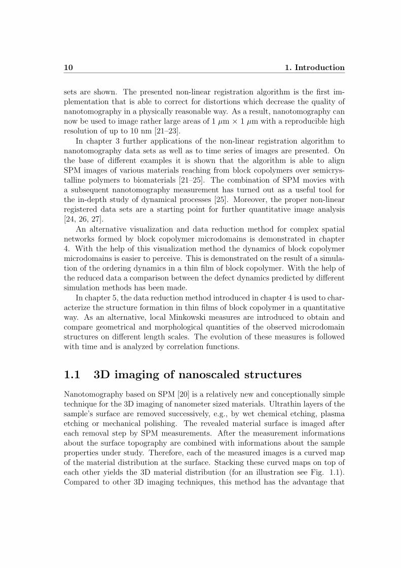
1.1 3D imaging of nanoscaled structures
Nanotomography based on SPM [20] is a relatively new and conceptionally simpletechnique for the 3D imaging of nanometer sized materials. Ultrathin layers of thesample’s surface are removed successively, e.g., by wet chemical etching, plasmaetching or mechanical polishing. The revealed material surface is imaged aftereach removal step by SPM measurements. After the measurement informationsabout the surface topography are combined with informations about the sampleproperties under study. Therefore, each of the measured images is a curved mapof the material distribution at the surface. Stacking these curved maps on top ofeach other yields the 3D material distribution (for an illustration see Fig. 1.1).Compared to other 3D imaging techniques, this method has the advantage that

1.1 3D imaging of nanoscaled structures 11
the depth resolution of the resulting 3D image is not dependend on the roughnessof the specimen and only limited by the local distance between two adjacent sur-faces and the surface sensitivity of the used SPM technique. With this method,3D images with a resolution of about 10 nm can be recorded [20, 22, 23, 28].With nanotomography it is possible to image the nanostructure of materials likesemicrystalline polymers [22] or submicron features of metallic alloys [28] whichcan not be recorded by transmission electron microtomography (TEMT) [29, 30],computerized tomography (CT) or conventional serial section methods.
Figure 1.1: Principle of nanotomography. With stepwise erosion of the surface aseries of curved maps S(n) is measured from which a volume image of the specimenis reconstructed. For details see text. (Adapted from [20]; c©2000 by the AmericanPhysical Society).
One problem of nanotomography is that SPM images are distorted by linear andnon-linear effects like hysteresis, creep, non-linearities of the feedback mechanism,or non-linear response of the piezo-scanner as well as thermal drift of the SPMsetup [18]. As the type and amount of these distortions differ from image to im-age, the reconstructed 3D material distribution has a poor quality. One method toovercome this problem is to compensate known scanner distortions by improvingthe measurement setup of the SPM (see, e.g., Refs. [31–37]). These improvementshave already been implemented in many modern SPMs. Nevertheless, some dis-tortions like thermal drift can not always be avoided, in particular, when no timefor thermal equilibration of the experimental setup is available or when older orlow cost instruments are used. In this thesis a post-experimental image processingmethod for the correction of non-linear distortions [21] is introduced as an alterna-tive method. This idea has already been used in previous works [11, 38, 39]. Sincethose methods correct only for (affine) linear distortions, they are not suited forcompensating for the distortions limiting the quality of nanotomography images.
For the registration of serial section images different linear as well as non-linearmethods have been developed in medical image processing (for reviews see, e.g.,

12 1. Introduction
Refs. [40–42]). Since the data acquisition of serial section methods in medicinediffers from SPM imaging, only very few of these non-linear registration algorithmsare suited for nanotomography. In this thesis, a two-dimensional (2D) curvaturebased registration algorithm developed by Fischer and Modersitzki [19] has beenmodified in order to handle particular problems occuring during the registration ofSPM data. The curvature registration algorithm delivers very smooth distortioncorrections. This is in good agreement with SPM measurements where distor-tions are relatively small and steady. The performance of the algorithm has beentested on several exemplary SPM data sets, e.g., the 3D micro-structure of a nickelbased superalloy [28], semicrystalline polymers [22], and human bone [23]. Thealgorithm worked well in all cases. The quality of the resulting 3D images hasbeen improved significantly (an example is shown in Fig. 1.2). Furthermore, thenon-linear registration algorithm can be applied to align 2D SPM image sequences[24, 26, 43]. By this a quantitative analysis of dynamical processes is now possibleand can be combined with nanotomography imaging to get further insight in thesephenomena.
Figure 1.2: (a) Isosurface of a crystalline lamella in elastic polypropylene after rigidregistration (b) cut through the gray value distribution after rigid registration atthe position indicated by the box in (a); (c) the same data set after curvaturebased registration; (d) cut through the gray value distribution after curvaturebased registration at the position indicated in (c). (Adapted from [21]; c©2006 bythe Institute of Physics).
Besides nanotomography further serial section methods can be applied to get 3Dimages of nanometer sized material distributions. Some of them work quite similarto the above described method [44, 45]. However, those methods do not take localheight information into account. For this reason, the depth resolution is limited.

1.1 3D imaging of nanoscaled structures 13
Alternatively, thin (i.e. 10-80 nm thick) slices are cut off the sample. These slicescan be imaged with high-resolution imaging techniques like transmission electronmicroscopy (TEM). After the measurement, all slices are aligned and are stackedto a 3D image [46]. These methods are very labor-intensive and also limited inresolution.
A second class of methods rely on the Radon transformation [47]. Here, aseries of 2D projections is acquired at different tilt angles of the specimen (foran illustration see Fig. 1.3(a)). Afterwards the original 3D density distribution isreconstructed (Fig. 1.3). For this different reconstruction algorithms exist [48–54].The most used method is the real-space weighted backprojection (see, e.g., Ref.[50]) which is very accurate.
Figure 1.3: Schematic illustration of the projection imaging process. (a) First,projections of the 3D material structure are taken at different tilt angles. (b) Forthe reconstruction of the 3D material distribution with a backprojection algorithmevery 2D projection is smeared out along the original beam angle. The differentbackprojections are superimposed to obtain an approximation of the original 3Dmaterial distribution. The more projections at different angles are taken the betteris the quality of the 3D reconstruction. (Adapted from Ref. [55]; c©1999 byAcademic Press).
Examples for this class are TEMT [29, 30] and CT. In TEMT projections of 3Dmaterial distributions are recorded by using an electron beam. The method isapplicable to relatively large structures (100-500 nm) yielding resolutions of 1-20nm. TEMT has been mainly applied to life science (see, e.g., Ref. [48, 56, 57])although there are also applications to material science (see, e.g., Ref. [52, 58–64]).
CT measurements are performed by using X-rays. Originally, CT scannershave been developed for medical applications (for a review of the development of

14 1. Introduction
medical CT scanners see, e.g., [65]). Modern micro- and nano-CT scanners havea resolution in the 0.3 µm range [66]. This makes CT more and more interestingfor non-medical applications like nondestructive material testing. However, theinvestigation of smaller structures is - as yet - not possible.
1.2 Visualization of 3D network structures
The view into reconstructed volume data sets is often obstructed as can be seen inthe data set displayed in Fig. 1.4. Prominent examples for materials which formsuch complex network structures on the nanometer scale are block copolymersand ordered mesophases of surfactants [67]. In nanotechnology, block copolymersare used for various applications like the development of high-density informationstorage media or photonic crystals [68]. They consist of two or more blocks ofimmiscible components which are covalently linked. This architecture leads to theformation of microdomains which contain only one of the blocks. To visualize thenanostructure of those materials often only small parts of the complete volumedata set are displayed as voxel (volume pixel) projections (see Fig. 1.4(a)) or byrendering of the isosurface (see Fig. 1.4(b)) [69]. A further method is to displaysingle cross sections through the 3D density distribution [70] (see Fig. 1.4(c)).Also dividing surfaces [71], skeletonization [72], and medial surfaces [73] are usedfor the visualization.
Figure 1.4: Demonstration of different visualization techniques for 3D volumedata sets on the example of a 3D nanotomography image of polystyrene-block -polybutadiene copolymer. Ten curved maps (size 256× 256 pixel) with a constantdistance of 7 nm are stacked on top of each other [43, 74]. Visualization by: (a)voxel projection, (b) isosurface (threshold ρ = 0.49), (c) slicing.
In this thesis, an alternative data reduction and visualization method for complexblock copolymer microdomain structures is introduced. Microdomains of cylinder-forming block copolymers are reduced to thin smooth lines. The branching points

1.3 Quantitative image analysis of nanostructured materials 15
are classified and marked by spheres of different color dependend on their connec-tivity (see Fig. 1.5). The method is applicable to 3D and 2D simulation data aswell as to 3D nanotomography or 2D SPM images. It is demonstrated on sim-ulation results of the ordering dynamics of microdomains in a thin film of blockcopolymer [75]. By compiling a complete series of the reduced data into a moviethe amount of data is significantly decreased while the relevant information is muchbetter perceivable.
Figure 1.5: Reduction of a gray scale image to a 2D network graph. In a firststep the image is binarized. The binary image is then skeletonized. Finally, theskeleton is reduced to a network graph.
1.3 Quantitative image analysis of nanostructured
materials
The classification and counting of branching points can also be used to follow thedynamics of block copolymer microdomains. For this purpose, the number of eachclassified branching point is counted for each image. Tracking the evolution ofthese numbers with time yields information about the rearrangement dynamics ofmicrodomains [26, 43].
For the quantitative analysis of microdomain structures further methods havebeen used in the literature. Harrison et al. studied experimentally the coarsen-ing dynamics in a single layer of cylinder-forming block copolymer microdomains[14, 15]. An orientation field of each image was computed by measuring localintensity gradients. By analyzing these orientation fields topological defects like±1
2disclinations (see Fig. 1.6) were detected. Additionally, the authors computed
orientational and translational order parameters and examined their temporal evo-lution by correlation analysis.
Segalman et al. studied the melting behavior of a hexagonally sphere formingdiblock copolymer on a topographically patterned substrate [16, 17]. Starting froma quasi-long-range ordered phase with few defects the temperature was increased.The hexagonal point pattern was analyzed by constructing the Voronoi diagram
16 1. Introduction
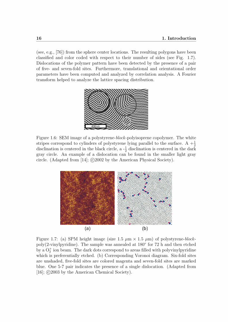
(see, e.g., [76]) from the sphere center locations. The resulting polygons have beenclassified and color coded with respect to their number of sides (see Fig. 1.7).Dislocations of the polymer pattern have been detected by the presence of a pairof five- and seven-fold sites. Furthermore, translational and orientational orderparameters have been computed and analyzed by correlation analysis. A Fouriertransform helped to analyze the lattice spacing distribution.
Figure 1.6: SEM image of a polystyrene-block -polyisoprene copolymer. The whitestripes correspond to cylinders of polystyrene lying parallel to the surface. A +1
2
disclination is centered in the black circle, a -12
disclination is centered in the darkgray circle. An example of a dislocation can be found in the smaller light graycircle. (Adapted from [14]; c©2002 by the American Physical Society).
Figure 1.7: (a) SPM height image (size 1.5 µm × 1.5 µm) of polystyrene-block -poly(2-vinylpyridine). The sample was annealed at 180 for 72 h and then etchedby a O+
2 ion beam. The dark dots correspond to areas filled with polyvinylpyridinewhich is preferentially etched. (b) Corresponding Voronoi diagram. Six-fold sitesare unshaded, five-fold sites are colored magenta and seven-fold sites are markedblue. One 5-7 pair indicates the presence of a single dislocation. (Adapted from[16]; c©2003 by the American Chemical Society).

1.4 Individual contributions to joint publications 17
Simulations of the coarsening of a two-dimensional block copolymer hexagonalphase have been analyzed by Vega et al. [77]. They computed orientational corre-lation lengths in a quite similar way to Segalman et al.. Furthermore, they trackedthe time evolution of correlation lengths which were determined from densities oftopological defects and from scattering functions.
Soille computed the orientation field of an image of a cylinder-forming blockcopolymer with the help of morphological operators [78]. Additionally, he usedthe watershed algorithm for the segmentation of different types of microdomains.He also computed local connectivity numbers and used them for the classificationand segmentation of different microdomain structures.
Another alternative for the classification of block copolymer microdomain pat-terns are Minkowski measures [79–81]. For 2D binary (i.e. black and white) imagesMinkowski measures are familiar geometrical and topological quantities: the whitearea fraction, the length of the boundary line between black and white regions, andthe Euler number which describes the topology of the (white) foreground structure.Minkowski measures are known to be robust, independent on statistical assump-tions on the distribution of phases, and can be calculated effectively [7, 82, 83]. Asduring the binarization of gray scale images a lot of information about the originaldensity distribution is lost, Minkowski measures often are computed for a set ofthresholds [83]. Comprising physical knowledge the resulting threshold dependend- and often redundant - curves can be reduced to a few characteristic parametersin a second step [7, 79]. As Minkowski measures are integral measures they arewell suited to capture global morphology transitions in a robust way [7, 8, 83–86]. However, small fluctuations which typically occur around individual defectsof block copolymer microdomains contribute only little to these global informationand are not captured by this kind of analysis.
In this thesis, the dynamics of block copolymer microdomains is analyzed bylocal Minkowski measures which are calculated for small areas centered aroundeach pixel. On the example of the Euler characteristic an intervall of thresholdsis identified where different block copolymer microdomain morphologies can bedistinguished in a robust way. The evolution of the Euler characteristic for oneconstant threshold is tracked with time and analyzed by correlation functions. Theresults of this analysis are compared to results obtained by computing pixel-to-pixel correlations and correlations of the time dependent numbers of branchingpoints.
1.4 Individual contributions to joint publications
Some chapters of this thesis have been published in collaboration with other au-thors. Therefore, my contributions to these publications are specified in the fol-

18 1. Introduction
lowing. The corresponding author is marked with an asterix. Due to my marriagein 2007 my name changed from Sabine Scherdel to Sabine Rehse.
• Chapter 2:This chapter has been published as ’Non-linear registration of scanningprobe microscopy images’ by S. Scherdel∗, S. Wirtz, N. Rehse and R.Magerle in Nanotechnology 17, 881 (2006). I have profited from a Matlabimplementation of the curvature algorithm written by Jan Modersitzki andfrom discussions with Stefan Wirtz about the block registration approach.From this starting point I have implemented the curvature block registrationalgorithm for the use with SPM images, the multi-resolution approach, andthe handling of image boundaries and artifacts. The method has been testedby me with two series of SPM images which have not been registered bythen. The results have been discussed and interpreted with Nicolaus Rehseand Robert Magerle. I have written the publication.
• Chapter 4:This chapter has been published as ’Visualizing the dynamics of com-plex spatial networks in structured fluids’ by S. Scherdel, H. G.Schoberth, and R. Magerle∗ in the Journal of Chemical Physics 127, 014903(2007). I have developed the ideas for the data reduction and visualiza-tion approach. Here, I have profited from discussions with Robert Magerle.The implementation of the 3D skeletonization algorithm has been done byme. Heiko Schoberth has implemented the algorithm for the conversion ofthe skeleton to a protein data base file (pdb file) and he has developed theempiric catalog for the handling of artifacts under my supervision. He hasalso performed the Mesodyn simulations. The draft and outline of the paperhave been written by all three authors. I have written the final publicationtogether with Robert Magerle.
• Chapter 5:This chapter has been submitted as ’Characterization of the dynamicsof block copolymer microdomains with local morphological mea-sures’ by S. Rehse∗, K. Mecke, and R. Magerle to Physical Review E.Christian Franke has implemented the algorithm for the calculation of localMinkowski measures under my supervision. The local Minkowski approachand the classification of branching points to experimental results of MarcusBohme have been applied by me. I have analyzed the results by correlationanalysis. The results have been discussed and interpreted with Klaus Meckeand Robert Magerle. I have written the publication.
Chapter 2
Non-linear registration of SPMimages1
Non-linear distortions caused by thermal drift and hysteresis of piezo-scannershinder the alignment of a series of two-dimensional scanning probe microscopy(SPM) images for nanotomography volume images and for movies. We report ona registration method to correct these distortions. To speed up the registration ofa complete stack of hundreds of two-dimensional images, the data were registeredin a whole block, and a multi-resolution approach was used. Other specific prob-lems of SPM measurements, such as image artifacts and the handling of imageboundaries, were solved by introducing a mask with implicit mapping. With thisapproach we are able to obtain high-resolution nanotomography images of modernnanostructured materials over large areas (1 µm × 1 µm) with a resolution of 10nm. Examples are individual crystalline lamellae in a semicrystalline polymer filmas well as a 50 nm wide channel in a nickel-based superalloy.
2.1 Introduction
Nanotomography is a new method to image the complex spatial structure of mod-ern materials in real space [20, 22, 28, 87]. The imaging process is similar to anexcavation on the nanometer scale: thin layers are stepwise removed from the spec-imen and each freshly exposed surface is imaged with scanning probe microscopy(SPM) [9, 88]. The resulting images R(n)(x1, x2) provide information about thematerial distribution of the specimen. Simultaneously height images z(n)(x1, x2)are measured which contain information about the shape of the surface after each
1This chapter has been published as: S. Scherdel, S. Wirtz, N. Rehse, and R. Magerle, Non-linear registration of scanning probe microscopy images, Nanotechnology 17, 881 (2006); c©2006by Institute of Physics.

20 2. Non-linear registration of SPM images
erosion step. Here, x1 and x2 are the usual spatial coordinates and n is the indexof the layer. By combining these two-dimensional images we obtain the materialdistribution on a curved surface. After recording all images, the stack of imageshas to be recombined to a volume image (Fig. 2.1). Hereby, the maps S(n) arestacked with a mutual distance according to the average erosion rate. During theSPM measurements unavoidable and in general non-linear distortions occur [18].As a result successive images do not lie exactly on top of each other, which reducesdrastically the image quality of volume images.
Figure 2.1: Principle of nanotomography. With stepwise etching a series of curvedmaps S(n) is measured from which a volume image of the specimen is reconstructed.For details see text. (Adapted from Ref. [20]; c©2000 by the American PhysicalSociety).
In this context, a particular problem is that the type and amount of image dis-tortions differ from image to image. Another application for the registration ofa series of two-dimensional images are SPM movies where distortions also reducethe imaging quality [89]. In this work we present a post-processing approach tocorrect image distortions in series of images for volume reconstruction.
An SPM image is acquired by successive scanning of parallel lines in the x1-direction. Each of these lines is scanned in the forward and in the backwarddirection. Superimposed to the fast tip motion in the x1-direction is a slowermotion in the x2-direction (Fig. 2.2). The resulting tip movement is a line-wisescanning of the area to be imaged. In an ideal case the points where data aretaken (the pixels) are located on an orthogonal grid.
However, a number of effects cause image distortions. The most important arehysteresis, creep and non-linear response of piezo-scanners, non-linearities of thefeedback mechanism, and thermal drift [18]. With a proper mechanical and elec-tronic design the influence of the different sources can be significantly minimized

2.1 Introduction 21
Figure 2.2: Schematic description of the relative tip movement during an SPMmeasurement. The bright pixels correspond to spots at which a measuring point(a pixel) is recorded; the dark lines show the path of the moving tip.
([31–37]; for a brief overview, see the introduction of [34]). In modern instrumentsmany of these design principles have been implemented. In practice, however,some image distortions always remain, in particular when older or low cost instru-ments with non-linearized piezo-scanners are used. The other major source forimage distortions is thermal drift which often occurs when the time for thermalequilibration of the experimental setup is not available.
Formally, the resulting image distortion can be described by an additionalvelocity component vd which adds to the scanning movement of the tip. As thescan rate along the fast scanning axis x1 is considerably faster than vd there arebarely distortions along the x1 axis. In the direction of the slow scan axis, however,the image can be distorted in a non-linear way.
As a result, post-processing of a series of images is required for the reconstruc-tion of high-resolution volume images. One example to correct a constant driftvelocity vd is to record an image of a crystal lattice with a known structure (e.g.,highly ordered pyrolytic graphite (HOPG)) and to calculate the deformation bymapping the measured grid on the known crystal structure. Under the assumptionthat the drift does not change during the measurements the obtained distortioncan be applied to all the following images [11]. Unfortunately, this method fails ifthe drift is not the same in each image, if the specimen is slightly shifted or rotatedbetween the recording of two successive images, or if images should be registered

22 2. Non-linear registration of SPM images
for which no reference grid was recorded.For periodic structures it is possible to determine the shape of the structure’s
unit cell by a Fourier transform. By mapping the unit cell of the image onto theexpected shape of the unit cell it is possible to determine the parameters for anaffine linear transformation of the image [38]. For non-periodic structures theseparameters can also be identified by fitting the shape of well-known geometricalfeatures [39]. These methods, however, have the disadvantage that they onlycorrect for linear deformations and are insufficient to correct for the non-lineardistortions.
In medical imaging, a wide palette of non-linear registration techniques hasbeen established for registration of serial sections obtained by, for example, mi-crotoming, computed tomography, and magnetic resonance imaging. It reachesfrom affine linear registration approaches (cross correlation, mutual information,principal axis based registration) over landmark based methods to non-parametricmethods like elastic registration and curvature based registration. For an overview,see, for example, [40–42].
We have modified the curvature based registration method of Fischer andModersitzki [19] for SPM data sets. The method is fast (O(N logN), where Nis the number of pixels in an image), yields smooth deformation grids, which arevery suitable to correct for the distortions occuring in SPM images, and does notdepend on an accurate pre-registration as do methods based on deformable models.
In the following we will briefly describe the 2D registration algorithm of Fischerand Modersitzki. Then we will go into details of our modifications and improve-ments, in particular the formulation of the curvature based registration as a 3Dwhole-block registration problem and the masking of boundaries and image arti-facts. Finally, we will give details on the choice of parameters during the numericalimplementation and present results for two exemplary data sets of nanotomogra-phy volume images [90].
2.2 The algorithm of Fischer and Modersitzki
There is a reference image R and a template image T . Without any restrictionΩ = [0, 1]2 is the area of registration. R(x) and T (x) correspond to the intensity ofthe 2D images at the point x = (x1, x2) ∈ Ω for the reference R and the templateT , respectively.
The aim of the registration is to find a deformation field u = (u1, u2) : Ω→ IR2
such that R(x) = T (x−u(x)). To express quantitatively how similar R and T area distance measure is introduced, for example, the sum of squared differences
D[R, T ; u] :=1
2
∫Ω
(T (x− u(x))−R(x))2 dx (2.1)

2.2 The algorithm of Fischer and Modersitzki 23
which corresponds to the squared L2-norm of the difference image
Du := Tu −R
withTu(x) = T (x− u(x)) for all x ∈ Ω.
Since the minimization of D[R, T ; u] yields no unique solution of the registrationproblem, a regularization term S[u] weighted with a factor α ∈ IR+ is added:
J [u] := D[R, T ; u] + α S[u] = min. (2.2)
The regularization term S[u] penalizes undesirable solutions and so favours solu-tions which obey an additional physical knowledge. In the case of curvature basedregistration this term reads
Scurv[u] :=1
2
2∑l=1
∫Ω
(∆ul)2dx, (2.3)
where ∆ =∂2
∂x21
+∂2
∂x22
is the Laplace operator.
As the curvature of the deformation enters (2.3), oszillating distortion gridsare penalized, which leads to very smooth solutions for the deformation field u.Since every affine linear transformation can be written in the form Ax + b withA ∈ IR2×2, b ∈ IR2, x ∈ Ω the second derivative of these deformations is zero.Consequently, such distortions are not penalized by Scurv[u]. This is also thereason why curvature based registration does not depend very much on linearpre-registration like methods based on deformable models (see, e.g., [40, 42]).
A necessary constraint for the minimization of J [u] is that the Gateaux deriva-tive disappears in all variational directions v, i.e.,
dJ [u; v] = limh→0
J [u + hv]− J [u]
h= 0 (2.4)
for all variations v : Ω→ IR2 with v = 0 on ∂Ω.With the special boundary conditions ∇ul = ∇∆ul = 0 for x ∈ ∂Ω, l = 1, 2
the relating Euler-Lagrange equation to the functional J is the non-linear partialdifferential equation (PDE)
f(x,u(x)) + α∆2u(x) = 0, x ∈ Ω, (2.5)
with
f(x,u(x)) = (R(x)− T (x− u(x)))∇T (x− u(x)) = −Du(x)∇T (x− u(x)).

24 2. Non-linear registration of SPM images
Equation (2.5) is also well-known as a biharmonic or bipotential equation. Sincef is a right-hand side of a PDE it is called force, driving the registration [19].
By approximating the partial derivatives through finite differences and by us-ing a time marching method one obtains a linear system of equations with 2Nunknowns where N is the number of pixels in an image. A particular choice ofboundary conditions allows to solve this huge linear system of equations by meansof a cosine transformation and to implement the algorithm with a complexity ofO(N logN) [19].
2.3 Registration of SPM images
2.3.1 Preprocessing
Before applying the curvature algorithm to the SPM data, the images are shiftedrigidly to reduce errors caused by up to 50 pixel large offset between the images.Each single translation was calculated by maximization of the cross correlationbetween two successive images.
One problem that was occuring when registering series of SPM images is thatthe recorded images do not always show the same area (Fig. 2.3). In general,the structure of the material to be analyzed is unknown. Therefore, the matchof the non-linear distorted image areas cannot be achieved by adequate cutting.After rigid pre-registration, the recorded images are shifted against each other. Ifthe original size of the images is maintained during the registration, in generalmost of the images will be shifted out of the initial display window. Due tothe non-periodic material structure it is not reasonable to use periodic boundaryconditions. Therefore, information is lost when the images are shifted out of theinitial display window after non-linear registration. To avoid this, we have addeda margin around each image and filled it with zeros in a first simple approach (Fig.2.4(a)).

2.3 Registration of SPM images 25
Figure 2.3: Tapping mode phase image of an etched surface of semicrystallinepolypropylene. The bright spots correspond to the crystalline regions, the darkspots to the amorphous parts (for details see [22]). The variation of the recordedimage window is displayed for two successive images in an exaggerated way. Typ-ical distortions are in the range of about 1-10% of the image size.
Figure 2.4: A tapping mode phase image as an example of non-linear registration.(a) Original image with margin, (b) non-linear registered image, (c) correspondingdeformation grid.
26 2. Non-linear registration of SPM images
2.3.2 Handling of boundaries and image artifacts
In the difference image Du only those parts contain reliable information that donot belong to the margin of any of the images contributing to the difference image,e.g., R and Tu. To distinguish which parts of the difference image contain reliableinformation we have used an implicit mapping. We shifted the range of gray valuesof the SPM images such that they do not contain pixels with zero value beforeadding the margin. For measuring the convergence rate we calculated the norm ofDu only over the area with reliable information and normalized it over the numberof pixels in this area.
During the calculation of u the distance measure only enters equation (2.5) byf [42]. It is only possible to calculate this term accurately in the area in whichthere exists reliable information for Du. On the other hand, the PDE (2.5) has tobe solved on the whole domain Ω. Therefore, it is necessary to extrapolate f. Wehave achieved this in a first approach by setting f equal to zero at spots with noreliable information.
This procedure can also be applied to artifacts which occur during many SPMmeasurements due to instabilities of the feed-back loop [91, 92], vibrations in theenvironment of the microscope, or by particles and residues caused by the etchingprocess itself. An implicit mapping is used to mask in each image spots withartifacts prior to the registration by a number which is not in the range of grayvalues of the image. The corresponding spots can be either masked manually orcan be identified automatically by choosing certain selection criteria. For example,shot noise like artifacts can be selected by setting a certain threshold value fromwhich on the data are not considered as reliable.
If the artifacts are inside of the domain with reliable data and if they are small(< 15 pixel) it is also possible to interpolate the data instead of filling the spotswith zeros. We have linearly interpolated each line containing artifacts betweenthe beginning and the end of the artifact area.
2.3.3 Whole block registration
The search for adequate values of α in (2.2) and the time step size τ of the timemarching method was a further problem. Since the contrast changes from layer tolayer the values for α and τ depend on the image data and had to be determinedfor each image. The pairwise registration of a complete data set of 20 layers took2-4 days even for a skilled operator. The solution of this problem was to formulatethe curvature based registration as a whole block approach, which until now wasonly done for elastic registration [93].
Here, there are not only two images R and T given but a whole stack of imagesR := (R(1), . . . , R(M)), R(ν) : Ω→ IR with Ω = [0, 1]2, ν = 1, . . . ,M, which have to

2.3 Registration of SPM images 27
be registered at once. In this way the values for α and τ have to be determined onlyonce for one complete series of images which eliminates the need to find the valuesfor each pair of images seperately. The aim is to find deformations u(ν) : Ω→ IR2,with ν = 1, . . . ,M , such that the distance
D[R,u] :=1
2
M∑ν=2
∫Ω
(R(ν)(x−u(ν)(x))−R(ν−1)(x−u(ν−1)(x))
)2dx (2.6)
becomes minimal.The regularization term is written in block notation
Scurv[u] :=1
2
M∑ν=1
2∑l=1
∫Ω
(∆u
(ν)l
)2
dx. (2.7)
The solution of the variational problem leads to the non-linear PDE
M∑ν=1
(f(ν) + α∆2u(ν)
)= 0 (2.8)
with
f(ν) :=(R(ν−1) ϕ(ν−1) − 2R(ν) ϕ(ν) +R(ν+1) ϕ(ν+1)
)∇R(ν) ϕ(ν),
ϕ(ν)(x) := x− u(ν)(x),
which can be solved analogously to (2.5) with only slight extensions.
2.3.4 Multi-resolution approach
To speed up the registration and to ensure a proper registration of major features inthe images we implemented a multi-scale approach [94]. The single layers are scaleddown to a fourth of their original size. The scaled down images are registered andthe result for u is used as the starting value for the registration of the images nextin scale. To avoid artifacts at the reduction process the images have to be filtereddue to the sampling theorem [95]. During this filtering image frequencies largerthan half the sample rate are removed. In this way contributions to the distancemeasure which derive from larger structures are emphasized, major image featuresare first registered, and the time-consuming calculation of local minima is reduced.
2.3.5 Implementation and results
The implementation of the algorithm was done in Matlab (MathWorks, Inc.; Ver-sion 7.0.1.24704). All results were calculated on a Windows XP computer with 1GB working memory and an Athlon 64 3200+ processor with 2.0 GHz.
28 2. Non-linear registration of SPM images
We have registered two different nanotomography data sets. The first onewas of elastic polypropylene (ePP) [22], and the second one was a nickel-basedsuperalloy CMSX-6 [28]. In both cases the SPM images were measured with aDimension 3100 SPM and Nanoscope 4 controller with a closed-loop for x1 and x2
direction (Veeco Instruments, USA). The samples were removed from the samplestage for each etching step. A coarse re-alignment of the samples was done by anoperator with the help of an optical microscope and a motorized stage.
Elastic polypropylene. - As a first application we registered a data set consistingof 22 SPM images of elastic polypropylene [22]. Here the individual layers wereremoved by wet-chemical etching and stored as (256×256) pixel sized TIFF images(16-bit gray scale). By adding an appropriate margin the images were resized to(312× 312) pixel (Fig. 2.4(a)).
Pre-registration decreased the distance measure by about 32 %. For non-linearregistration (with α = 300 000 and τ = 0.5) we used the described multi-resolutionapproach with a three-step Gauß pyramid. For the scaled-down images we calcu-lated 15 iterations, and for the original-sized images 50 iterations. The wholeregistration process took 8 min and decreased the distance measure furthermoreby about 48 %. In comparison with the only rigidly registered image there aremany more details recognizable even in areas that are distant from the center of ref-erence of the linear registration (Fig. 2.5). In the rigidly registered data set shownin Fig. 2.5(a), the shift is still larger than the observed structures. Thereby, theinterpolation between the layers yields no coherent lamella. After non-linear reg-istration, however, the interpolation between the layers yields a connected lamella(Fig. 2.5(c)). Also the borders of the lamella are smoother though small shiftsseem to remain. In this way non-linear registration enables us to see more detailseven over large volumina (Fig. 2.6). The effect is better seen comparing the crosssections in Fig. 2.5(b) and Fig. 2.5(d). Strictly speaking our algorithm minimizesdrastic changes between neighboring images. The resulting volume image may stillcontain a global distortion which does not disturb the quality of the volume image.
As there are very different results dependend on the choice of α and τ , it wasimportant to inspect the registration results (Fig. 2.4(b)) by an expert. To doso, we depicted the calculated distortions by a deformation grid (Fig. 2.4(c)). Asthere are barely distortions along the fast scan axis the horizontal lines of thedeformation grid should preferably lie on a straight line. Along the slow scan axis,however, the deformation grid can be slightly curved.
For detecting an optimal α we began with a very large α. We had very smoothand stable solutions due to the dominating influence of the regularization term. Toachieve a further decrease of the error we reduced α stepwise. An α was declaredas too small when the horizontal lines in the deformation grid were no longersufficiently smooth. The step size τ of the time marching method was chosen togive a monotonic decrease of the error curve which should be preferably steep.

2.3 Registration of SPM images 29
Figure 2.5: (a) A part of the data set shown in Fig. 2.6 after rigid registration;(b) cut through the gray value distribution after rigid registration at the positionindicated by the box in (a); (c) the same data set after curvature based registration;(d) cut through the gray value distribution after curvature based registration atthe position indicated in (c)
After registration not all lamellae are perpendicular to the surface of the speci-men and there are lamellae connecting in tilted angles (Fig. 2.7). Since this is

30 2. Non-linear registration of SPM images
Figure 2.6: Nanotomography image of the crystalline regions of ePP (the samedata set is shown in Ref. [22] from another perspective.)
likely to occure in reality, this is a further demonstration of the plausibility of theregistration method and the choice of parameters.
Figure 2.7: Cross section through an ePP film displaying the different orientationsof crystalline lamellae. The bright areas represent the crystalline lamellae, and thedark areas indicate the amorphous areas of the material.
Nickel-based superalloy CMSX-6. - Another application of our registration methodconcentrated on a material of a different kind. Here a nickel-based superalloy(Ni3Al/Ni alloy CMSX 6) was analyzed, which was stepwise eroded by chemo-mechanical polishing (Fig. 2.8(a)). This data set had just been rigidly regis-tered up to now [28]. The 16 recorded images have a size of (512 × 512) pixelswhich rescaled after adding the margin to (776× 776) pixels. By using rigid pre-registration, the distance measure was decreased by about 28 %. The subsequent

2.4 Conclusions 31
non-linear registration with α = 900 000, τ = 0.4, and a three-step Gauß pyramidwas carried out with 15, 15, and 30 iterations, respectively. It reduced the distancemeasure by further 57 % and took only 31 minutes.
Compared with the only rigidly registered image there are significant improve-ments. Beside the overall smoother contours in the non-linear registered image it ispossible to recognize fine material structures, for example, a 50 nm wide channel(Fig. 2.8(c)), which were barely identifiable before non-linear registration (Fig.2.8(b)).
Figure 2.8: (a) Topographic image of the Ni3Al/Ni alloy CMSX 6 after chemo-mechanical polishing. The bright areas correspond to the Ni phase, the dark areasto the Ni3Al phase. The bright box indicates the spot which contributes to the3D data set displayed in ((b),(c)). ((b),(c)) Nanotomography image of the Ni3Alphase after rigid (b) and non-linear (c) registration of the 2D data
2.4 Conclusions
We have applied a registration algorithm developed in medical imaging scienceto SPM images. Despite the different field of application we could improve thequality of nanotomography data sets in a physically reasonable way. Furthermore,we have combined the curvature based registration algorithm with whole-blockregistration, which significantly increases the registration rate. Stacks of hundredsof 2D images can now be registered in a reasonable time.
This reduction of the computational costs allows us to interpret the parametern as a time value and to apply our registration algorithm to SPM movies withhundreds of images. As a result, the image quality of movies, like, for instance, the

32 2. Non-linear registration of SPM images
dynamics of structural phase transitions in ordered fluids [89], can be considerablyincreased, though global image distortions may remain.
Non-linear image registration gives way to obtain volume images and moviesof modern materials in real space with a resolution of 10 nm. This allows fornew insights into the microstructure and dynamics of nanostructured materialswhich cannot be obtained whithout the application of an appropriate registrationmethod.
2.5 Acknowledgements
We thank S. Marr for help with data acquisition. We also thank B. Fischer and J.Modersitzki for discussions and the intruduction to their registration algorithm.Finally, we thank the VolkswagenStiftung for generous financial support.
Chapter 3
Further applications of imageregistration
The non-linear registration method which was introduced in chapter 2 has beenused to improve the quality of nanotomography images of different materials in-cluding elastomeric polypropylene (ePP), block copolymers, and biomaterials. Theresulting volume images give new insights into physical phenomena like the growthof individual crystalline lamellae in ePP or into the material distribution of mate-rials which can not be obtained by conventional methods. Additionally, sequencesof images (movies) have been aligned. As a result, dynamic processes on thenanometer scale like the growth of individual crystallites or the rearrangement ofblock copolymer microdomains can be studied and quantitatively analyzed withunprecedented temporal and spatial resolution.
3.1 Semicrystalline polypropylene
Elastomeric polypropylene (ePP) is a material whose nano-structure is composedof small crystallites that are embedded in an amorphous matrix [108]. The num-ber and the spatial arrangement as well as the connectivity of the nanometer sizedcrystallites has large influence on the physical properties of the material. There-fore, the crystallization process has been studied with various methods [108–112].However, all of these methods are either 2D measurements of the surface or giveonly information on the average volume structure of the material. 3D imaging ofePP is difficult because of the small size (≈ 10 nm) of individual crystallites. Inrecent studies polypropylene has been imaged in 3D by TEMT [64] and nanoto-mography [22] (see also chapter 2).
ePP has been used to further demonstrate the reliability of non-linear registra-tion for SPM images. For this purpose, the same spot of an already crystallized

34 3. Further applications of image registration
ePP specimen was imaged over a time span of about 4 h taking an image every3 min [74] (see Fig. 3.1). A tool for an automized correcture has been used tocorrect for translational drift of the instrument [23].
Figure 3.1: Examples of SPM phase images of ePP imaged at the same spot for over4 h. The light areas correspond to crystalline regions. The dark areas correspondto the amorphous phase [74].
By this, the same structure was imaged, only distorted by the instruments noiseand drift. The effects of the SPM drift can be visualized by stacking the measuredimages to a 3D image using a commercial software (Amira 4.0, Mercury ComputerSystems). This 3D image can be analyzed by applying cross sections along thetime axis (Fig. 3.2). As can be seen, slight shifts of the layers occur during themeasurement. For this reason, there are no straight gray lines in x-t sections asone would expect (Fig. 3.2(a)). Even after linear pre-registration (Fig. 3.2(b)) thelines look like a zipper due to non-linear distortions caused by different directions ofthe slow scan axis. After non-linear registration of the image series (size 336×336pixels, parameters α = 70 000, τ = 0.3, four-step Gaussian pyramid with 30, 30,20, and 100 iterations, respectively) the gray lines in the x-t section are lined upalmost perfectly (Fig. 3.2(c)). The computation time was 1 h 2 min on an AMDAthlon 64 X2 Dual Core 4400+ (2.1 GHz, 2 GB RAM). In the correspondingdeformation grids (for one example see Fig. 3.3) all horizontal lines are straightwhereas the vertical lines are slightly curved. No crystallite structure is visible inany deformation grid. This is in good accordance to physical reasonable distortions(see chapter 2).

3.1 Semicrystalline polypropylene 35
Figure 3.2: Stack of 82 SPM phase images corresponding to Fig. 3.1 displayed bya cut in x-t direction. (a) Original data (aligned by an automized tool for lateralalignment during the measurement), (b) linear pre-registered data, (c) non-linearregistered data.
Figure 3.3: Example of a deformation grid according to the non-linear registrationof the data shown partly in Fig. 3.1. Note that the grid lines are slightly curved.

36 3. Further applications of image registration
The curvature registration method has also been applied to in-situ SPM crys-tallization studies recently carried out by Franke et al. [25]. After a linear pre-registration the 84 measured SPM images (size 462 × 462 pixels) have been non-linearly registered with parameters α = 50 000 and τ = 0.05. A two-step Gauß-pyramid was used. 100 and 15 iterations, respectively, have been computed. Thetotal computation time of the non-linear registration was 2 h 38 min on an AMDAthlon 64 3200+ (2.2 GHz, 1 GB RAM).
In the resulting image sequence the growth of crystalline lamellae can be fol-lowed in an area of about 2 µm × 2 µm with a temporal resolution of 3 minper frame. Concentrating on individual lamellae, the authors observed differentcrystallization phenomena (Fig. 3.4).
Figure 3.4: Detail of a series of SPM phase images displaying the crystallizationprocess of one lamella. Bright areas correspond to crystalline lamellae, dark areasto the amorphous phase. (a) 16 min, (b) 37 min, (c) 75 min, and (d) 264 min afterquenching. (From Ref. [25]; c©2007 by the American Chemical Society).
One of them was a lamella that grows continuously at the beginning of the obser-vation. After 1.5 h the lamella starts to thicken at one spot. At the end of themeasurement two separate lamella with parallel orientation are observed. Phenom-ena like this can not be sufficiently explained by considering only 2D informationsacquired at the surface. To gain further insight into the crystallization process,a nanotomography image of the observed area has been captured after the crys-tallization study. By wet chemical etching (for details see Ref. [22]) 42 layers(size 234 × 234 pixels) of the specimen have been removed. The measured SPMimages have been registered by curvature registration (parameters α = 500 andτ = 0.000001, 417 and 15 iterations, respectively, two-step Gauß-pyramid). The
3.1 Semicrystalline polypropylene 37
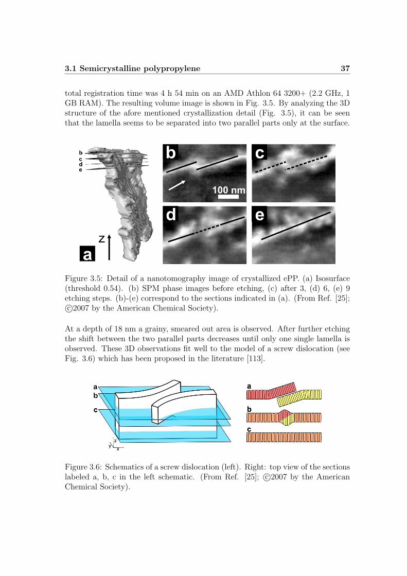
total registration time was 4 h 54 min on an AMD Athlon 64 3200+ (2.2 GHz, 1GB RAM). The resulting volume image is shown in Fig. 3.5. By analyzing the 3Dstructure of the afore mentioned crystallization detail (Fig. 3.5), it can be seenthat the lamella seems to be separated into two parallel parts only at the surface.
Figure 3.5: Detail of a nanotomography image of crystallized ePP. (a) Isosurface(threshold 0.54). (b) SPM phase images before etching, (c) after 3, (d) 6, (e) 9etching steps. (b)-(e) correspond to the sections indicated in (a). (From Ref. [25];c©2007 by the American Chemical Society).
At a depth of 18 nm a grainy, smeared out area is observed. After further etchingthe shift between the two parallel parts decreases until only one single lamella isobserved. These 3D observations fit well to the model of a screw dislocation (seeFig. 3.6) which has been proposed in the literature [113].
Figure 3.6: Schematics of a screw dislocation (left). Right: top view of the sectionslabeled a, b, c in the left schematic. (From Ref. [25]; c©2007 by the AmericanChemical Society).

38 3. Further applications of image registration
3.2 Block copolymers
Block copolymers are used for different applications like antireflexion coatings [96],nanowires [97], or lithographic purposes [68]. They consist of at least two immisci-ble polymeric chains (blocks), which are covalently bond. Due to repulsive interac-tions between the blocks a phase segregation takes place. As the polymeric chainsare chemically linked, this phase segregation can only take place on a mesoscopiclength scale (≈ 10-100 nm). Dependend on the volume fraction of the individ-ual blocks, the interaction between the blocks, and the degree of polymerizationdifferent microdomain structures can form (e.g., spheres, cylinders, or lamellae)[67].
Kreis [24] has studied a cylinder forming polystyrene-block -polybutadiene co-polymer. For the polystyrene block the glass transition temperature is above roomtemperature what means that the polymer does not move at this temperature. Toinduce mobility to the system, it is possible to heat the sample above the glasstransition temperature [157] or to use an unselective solvent to swell the blockcopolymer [24, 99]. In both cases, the now mobile block copolymer is able to formlong range ordered structures of microdomains. In a confined geometry, e.g., a thinfilm, the formation of these structures is influenced by the energies of the additionalinterfaces and by the film thickness. Despite the more complex interactions, thequasi 2D structure of a thin film allows to capture the dynamical rearrangementsof the microdomains in the thin film by studying its surface with an SPM.
A thin film of polystyrene-block -polybutadiene on a mica substrate has beenmeasured in a swollen state by Kreis with an SPM [24]. After swelling with chloro-form vapor the polymer film has a thickness of 32 nm which corresponds approxi-mately to the thickness of one layer of polystyrene cylinders. The obtained SPMimages have been converted to 16-bit gray scale TIFF images and subsequentlythe histograms of the images have been equalized [24]. Additionally, the imageshave been filtered by a low pass filter that removed features smaller than 8 nm.Due to non-linear image distortions individual features have been slightly shiftedfrom one image to another. This makes it difficult to discriminate the movementswhich originate from the microdomains themself from the jitter that originates inimage distortion.
For this purpose, all SPM images have been registered with the method de-scribed in chapter 2. The parameters of the non-linear registration method havebeen chosen as α = 50 000 and τ = 0.3. 40 iterations have been computed. Thetotal registration time for 258 images (size 496× 496 pixels) has been 3 h 41 minon an AMD Athlon 64 3200+ (2 GHz, 1 GB RAM) [98]. After the registrationprocess the information contained in the SPM movie was much better perceivable.The image processing allowed for an easier detection of different phenomena likea ring dot defect which shows peristaltic fluctuations (Fig. 3.7) or the meander-

3.2 Block copolymers 39
ing of a group of cylinders (Fig. 3.8) which are subject to further experimentalinvestigation.
Furthermore, the improved alignment of the SPM images opens the possibilityto visualize the temporal evolution of the measured microdomains by interpretingthe time axis as the third dimension of a 3D volume image (Fig. 3.9) [24]. In thisway, e.g., the fluctuation behavior of cylinder thicknesses can be directly observed.Furthermore, a good alignment of block copolymer microdomain structures makesit possible to analyze the dynamics of individual defects and to correlate themwith changes in experimental parameters [26].
Figure 3.7: SPM phase images of a thin polystyrene-block -polybutadiene film mea-sured in chloroform vapor on a mica substrate. The bright areas correspond tomicrodomains of polystyrene. A dot-like polystyrene bead (white arrows) is mov-ing around a defect structure in the middle of the images. At each time a differentangle can be assigned to the wandering bead (From Ref. [24]).
Figure 3.8: SPM phase images of a thin polystyrene-block -polybutadiene film mea-sured in chloroform vapor on a mica substrate. The bright lines correspond tocylinders of polystyrene. During the observation the cylinders performed mean-dering movements which are indicated by the red lines. The time between theimages was 63 s for the first two images and 26 s for the second and the thirdimage (From Ref. [24]).
40 3. Further applications of image registration
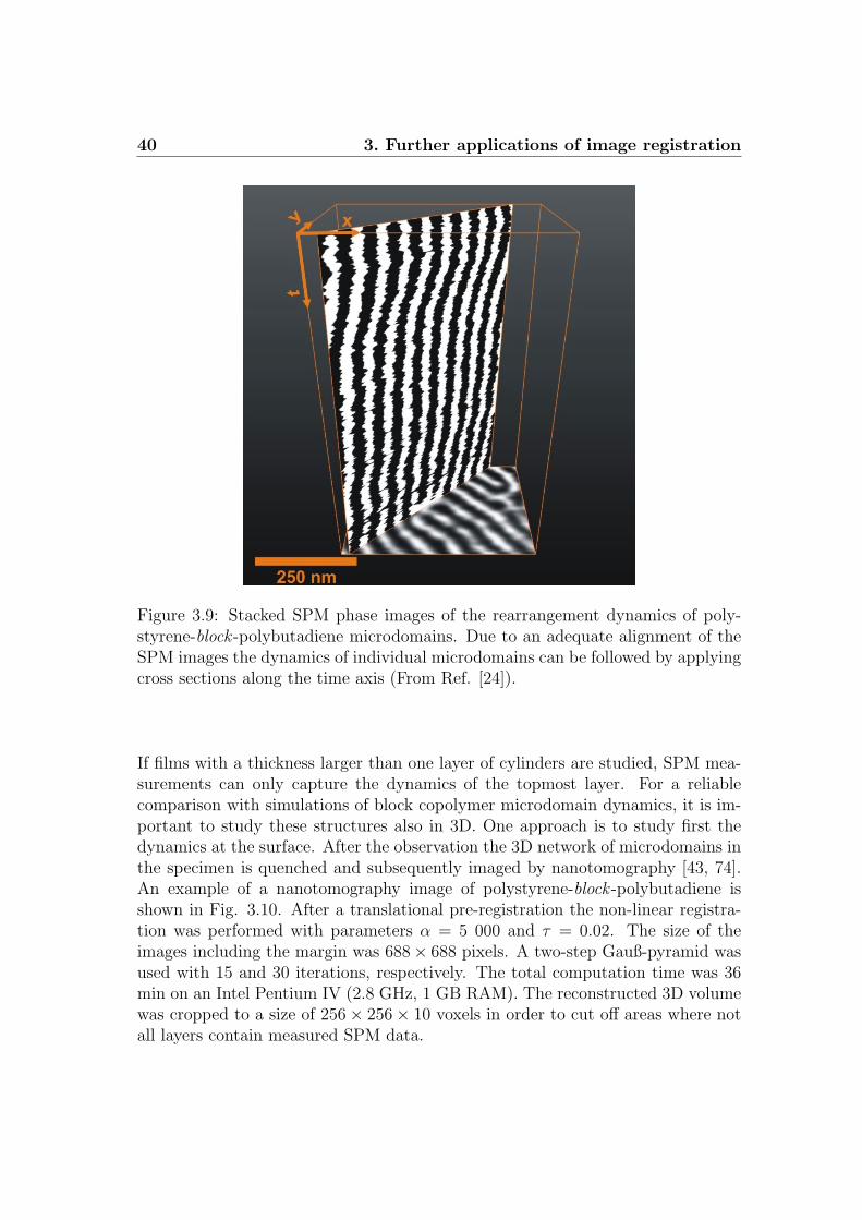
Figure 3.9: Stacked SPM phase images of the rearrangement dynamics of poly-styrene-block -polybutadiene microdomains. Due to an adequate alignment of theSPM images the dynamics of individual microdomains can be followed by applyingcross sections along the time axis (From Ref. [24]).
If films with a thickness larger than one layer of cylinders are studied, SPM mea-surements can only capture the dynamics of the topmost layer. For a reliablecomparison with simulations of block copolymer microdomain dynamics, it is im-portant to study these structures also in 3D. One approach is to study first thedynamics at the surface. After the observation the 3D network of microdomains inthe specimen is quenched and subsequently imaged by nanotomography [43, 74].An example of a nanotomography image of polystyrene-block -polybutadiene isshown in Fig. 3.10. After a translational pre-registration the non-linear registra-tion was performed with parameters α = 5 000 and τ = 0.02. The size of theimages including the margin was 688× 688 pixels. A two-step Gauß-pyramid wasused with 15 and 30 iterations, respectively. The total computation time was 36min on an Intel Pentium IV (2.8 GHz, 1 GB RAM). The reconstructed 3D volumewas cropped to a size of 256× 256× 10 voxels in order to cut off areas where notall layers contain measured SPM data.

3.2 Block copolymers 41
Figure 3.10: Isosurface (threshold ρ = 0.49) of a 3D nanotomography image ofpolystyrene-block -polybutadiene copolymer. Ten curved maps (size 256× 256 pix-els) with a constant distance of 7 nm are stacked on top of each other [43, 74].
Self-assembly of block copolymers typically leads to only short range ordered mi-crodomain structures. Therefore, external fields are often used to yield a macro-scopic orientation [100–106]. Olszowka et al. have developed a method towardsa long-range ordered stripe pattern [103]. For this purpose, the authors used alamella forming ABC triblock terpolymer with a short middle block B. The mid-dle block is adsorbed onto the substrate and acts as an anchor. The two majorityblocks then form a striped pattern. Initially, this pattern exhibits only short rangeorder. To induce long range order an in-plane electric field is applied to the poly-mer. Under the influence of this field domains of highly ordered stripes form whichare parallel to the electric field vector. The structural evolution of the alignmentwas studied with quasi in-situ SPM measurements [107] (see Fig. 3.11). The 26measured SPM images (size 700× 700 pixels) first have been corrected for lateraloffsets by applying a translational pre-registration.
Subsequently, the images have been non-linearly registered. The registration pa-rameters have been chosen as α = 1 000 000 and τ = 0.05. 20 iterations havebeen calculated. As a result, the alignment of the block copolymer lamella canbe observed with high resolution in a large area (Fig. 3.11). For the analysis ofindividual defects small areas can be cut out at arbitrary positions (Fig. 3.12).
.

42 3. Further applications of image registration
Figure 3.11: Series of SPM images showing the transition from a disordered struc-ture (a) to a highly ordered stripe pattern (g) (scale bar: 200 nm). The blockcopolymer film was annealed in saturated vapor at an electric field of 15 V µm−1
in a quasi in-situ SPM chamber. (From Ref. [103]; c©2006 by the Royal Societyof Chemistry).
Figure 3.12: Detail of the SPM images shown in Fig. 3.11 displaying a group ofdefects which dissolve to the end of the measurement almost completely. Addi-tionally, the defect annihilation is shown by some schematics below. (From Ref.[103]; c©2006 by the Royal Society of Chemistry).
3.3 Bones
Bone is a biological composite material with a highly complex structure fromthe millimeter down to the nanometer scale. It is composed of small inorganicparticles of hydroxyapatite (≈ 65% of the material) which are embedded in anorganic matrix of collagen (≈ 35% of the material) [114]. Although the structure

3.4 Conclusion 43
of bones is well studied on a scale reaching from millimeters down to 10 µm [115],there is not much information about its 3D nanostructure up to now [23, 116].However, the structure of bones on a scale reaching from 10-100 nm is importantfor its mechanical properties [117–120]. In particular, diseases of bones can asyet only be recognized when the structure damage is visible on the micron ormillimeter scale. It is supposed that the degeneration of the bone structure startson the nanometer scale. The possibility to recognize potential bone diseases inearly states would offer new forms of therapies. Furthermore, knowledge aboutthe exact composition of bones on the nanometer scale can help to create newbio-inspired materials.
Roper has studied the structure of cortical ovine and human bones with nano-tomography during her diploma thesis [121]. As an example, a 3D volume imageof human bone has been obtained [23]. The specimen has been etched with a 0.1M solution of HCl (for details of the preparation and etching see Refs. [23, 121]).19 layers (size 256×256 pixels) have been recorded by in-situ SPM measurements.The linearly pre-registered SPM phase images have been registered by curvatureregistration (parameters α = 500 000 and τ = 0.02, two-step Gauß-pyramid, 15iterations at each resolution). The total registration time was 20 min on an AMDAthlon 64 3200+ (2.2 GHz, 1 GB RAM) [122].
The obtained volume image has been visualized with the help of isosurfaces(see Fig. 3.13). As the observed structures can not be assigned to any knownstructural element the interpretation of the obtained 3D images is still subject toactual research.
3.4 Conclusion
In this chapter various applications of curvature based non-linear registration toSPM images have been demonstrated. It has been shown that the method isapplicable to SPM images of a broad field of materials. These materials can nowbe imaged with high resolution over large areas what was not possible before. It hasimproved the quality of 3D nanotomography data sets as well as the quality of 2DSPM movies displaying rearrangement processes of block copolymer microdomainsor the crystallization of ePP. By combining the information gained from non-linearaligned movies with high resolution nanotomography imaging, new insights intoseveral crystallization mechanisms of ePP have been obtained. Moreover, propernon-linear registration opens the way for quantiative image analysis of 3D datasets as well as of 2D movies [22, 24, 26, 27, 123].
Nanotomograhy studies of other materials are possible in future work, e.g.,the study of polymer solar cells [124], organic light emitting devices [125], ma-terials which are reinforced with nanoparticles, e.g., carbon nanotubes [126], or

44 3. Further applications of image registration
Figure 3.13: 3D isosurface image (threshold 0.62) of human bone (size 256×256×19) etched with a 0.1 molar solution of HCl. The distance between the individuallayers is about 15 nm. (From Ref. [23]; c©2007 by the American Institute ofPhysics).
other biological materials, e.g. teeth or cartilage. Non-linear registration may alsohelp to identify structural changes during strain-stress experiments of ePP on thenanometer scale which is subject to current research in our group [127, 128].

Chapter 4
Visualizing the dynamics ofcomplex spatial networks instructured fluids2
We present a data reduction and visualization approach for the microdomain dy-namics in block copolymers and similar structured fluids. Microdomains are re-duced to thin smooth lines with colored branching points and visualized with atool for protein visualization. As a result the temporal evolution of large volumedata sets can be perceived within seconds. This approach is demonstrated withsimulation results based on the dynamic density functional theory of the orderingof microdomains in a thin film of block copolymers. As an example we discuss thedynamics at the cylinder-to-gyroid grain boundary and compare it to the epitax-ial cylinder-to-gyroid phase transition predicted by Matsen [M. W. Matsen, Phys.Rev. Lett. 80, 4470 (1998)].
4.1 Introduction
Block copolymers and ordered mesophases of surfactants form spatially complexstructures on the nanometer scale [67]. These materials have attracted a large in-terest as templates for the synthesis of nanostructures of inorganic materials [68].Furthermore interesting similartities exist to biomembranes [130] and intracellularcompartments in living cells [131]. In the past decade different experimental tech-niques such as electron tomography [58, 61] and nanotomography [20] have beendeveloped to obtain volume images of these structures with 10 nm resolution.
2This chapter has been published as: S. Scherdel, H. G. Schoberth, and R. Magerle, Visual-izing the dynamics of complex spatial networks in structured fluids, Journal of Chemical Physics127, 014903 (2007); c©2007 by the American Institute of Physics.

46 4. Visualizing the dynamics of complex spatial networks
At the same time advances in theory and simulation methods allow us to pre-dict the structure and dynamics of these systems [132]. Of particular interestfor the understanding of the structure formation processes is the spatial structureof individual defects and grain boundaries and their dynamics during shear flow[133–135], structural phase transitions [89, 137, 138], and their behavior in electricfields [61, 61, 139–144].
The typical simulation result is the spatiotemporal evolution of the densitydistribution of block copolymer components within the simulated volume. Thedata set consists of several thousand snapshots of such density distributions (Fig.4.1). Fig. 4.1(a) shows the density distribution on the boundary of the simulatedvolume. The task is to also display the internal structure within the simulated vol-ume, to do this for all time frames and to enable the viewer to perceive the spatiallycomplex structures as well as their temporal evolution. Because of the large num-ber of available time frames, methods are needed which allow for a fast reception ofthe spatially complex dynamics. The techniques to display three-dimensional datasets either with two-dimensional projections or on stereo displays are called vol-ume rendering [136]. The conventional approaches to visualize threedimensionalblock copolymer microdomain structures are isodensity surfaces (Figs. 4.1(b) and(c)). Because the typical volume fraction of the material is in the 30%-50% regime,meaningfull isodensity threshold values give rather dense networks which obstructthe view into the simulation box.
A common way to overcome these visualization problems is to crop the volumeand display only small parts of the entire structure [69]. An alternative is todisplay only a two-dimensional cross section through the volume data set [70]or to restrict oneself to the study of two-dimensional or quasi-two-dimensionalsystems [89, 137, 138, 141, 144].
A direct volume rendering using an appropriate transparency map [136] is alsonot suitable for an easy reception and recognition of block copolymer microdomainstructures in large volumes because of the rather smooth density variations. Alter-native representations of microdomain structures are intermaterial dividing sur-faces [71], the reduction of microdomains to their skeleton [72], and medial surfaces[73].
In this work we present a method to perceive the spatially complex dynamicsin block copolymers and other structured fluids. The method consists of twosteps. First the microdomain structures are reduced to their minimal features:connections are represented as thin smooth lines and branching points as smallspheres of different colors. The resulting network and its dynamics are visualizedwith a tool for protein visualization. As a result, the viewer can perceive largedata streams with hundreds of volume images within seconds when displayed asan animated sequence of images (movie). As an example, we present the dynamics
4.2 Method 47
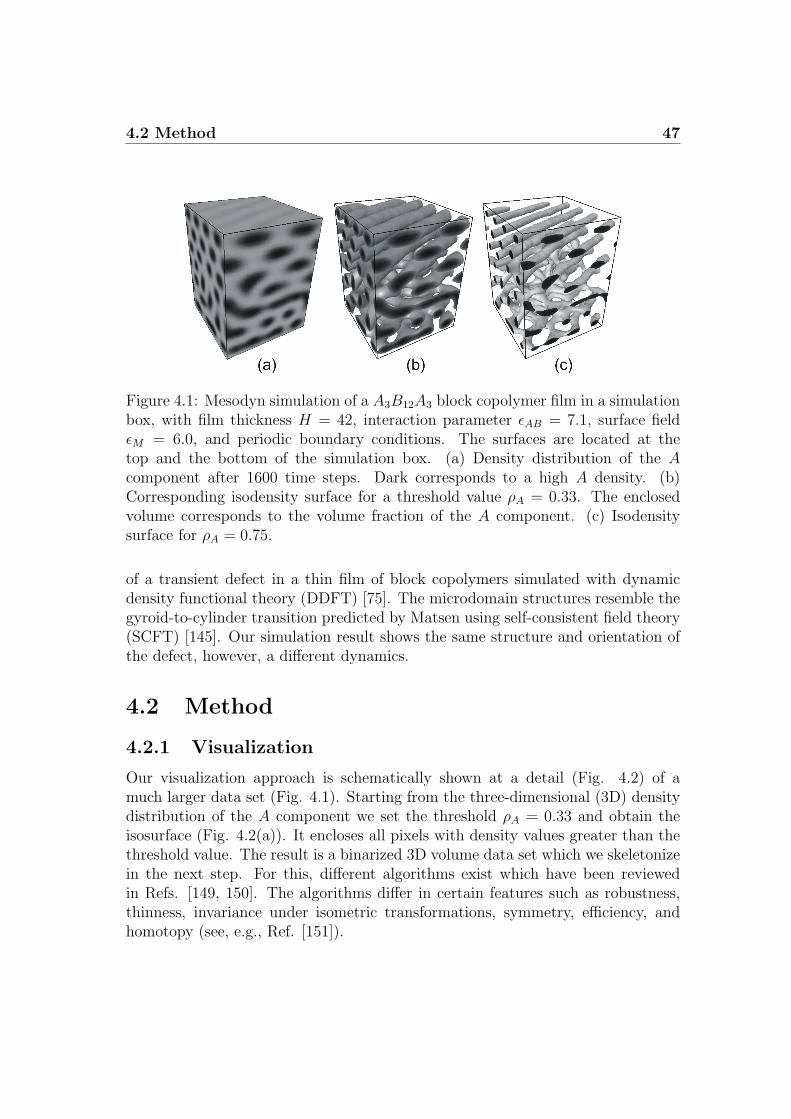
Figure 4.1: Mesodyn simulation of a A3B12A3 block copolymer film in a simulationbox, with film thickness H = 42, interaction parameter εAB = 7.1, surface fieldεM = 6.0, and periodic boundary conditions. The surfaces are located at thetop and the bottom of the simulation box. (a) Density distribution of the Acomponent after 1600 time steps. Dark corresponds to a high A density. (b)Corresponding isodensity surface for a threshold value ρA = 0.33. The enclosedvolume corresponds to the volume fraction of the A component. (c) Isodensitysurface for ρA = 0.75.
of a transient defect in a thin film of block copolymers simulated with dynamicdensity functional theory (DDFT) [75]. The microdomain structures resemble thegyroid-to-cylinder transition predicted by Matsen using self-consistent field theory(SCFT) [145]. Our simulation result shows the same structure and orientation ofthe defect, however, a different dynamics.
4.2 Method
4.2.1 Visualization
Our visualization approach is schematically shown at a detail (Fig. 4.2) of amuch larger data set (Fig. 4.1). Starting from the three-dimensional (3D) densitydistribution of the A component we set the threshold ρA = 0.33 and obtain theisosurface (Fig. 4.2(a)). It encloses all pixels with density values greater than thethreshold value. The result is a binarized 3D volume data set which we skeletonizein the next step. For this, different algorithms exist which have been reviewedin Refs. [149, 150]. The algorithms differ in certain features such as robustness,thinness, invariance under isometric transformations, symmetry, efficiency, andhomotopy (see, e.g., Ref. [151]).
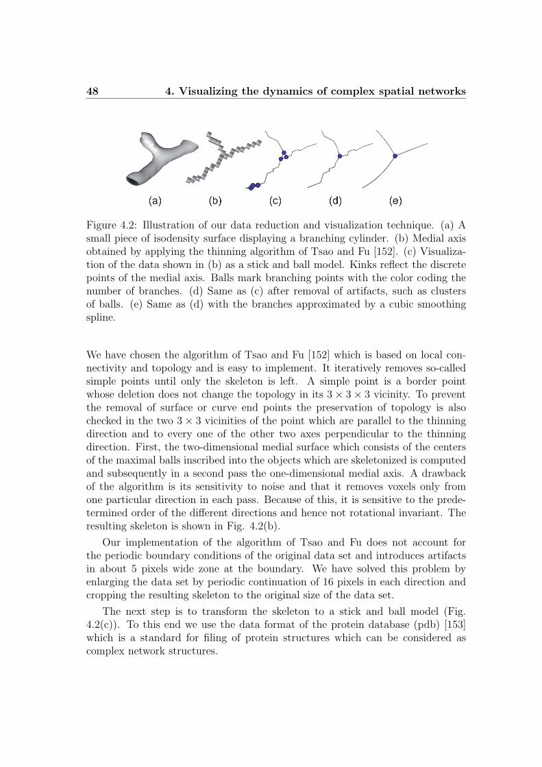
48 4. Visualizing the dynamics of complex spatial networks
Figure 4.2: Illustration of our data reduction and visualization technique. (a) Asmall piece of isodensity surface displaying a branching cylinder. (b) Medial axisobtained by applying the thinning algorithm of Tsao and Fu [152]. (c) Visualiza-tion of the data shown in (b) as a stick and ball model. Kinks reflect the discretepoints of the medial axis. Balls mark branching points with the color coding thenumber of branches. (d) Same as (c) after removal of artifacts, such as clustersof balls. (e) Same as (d) with the branches approximated by a cubic smoothingspline.
We have chosen the algorithm of Tsao and Fu [152] which is based on local con-nectivity and topology and is easy to implement. It iteratively removes so-calledsimple points until only the skeleton is left. A simple point is a border pointwhose deletion does not change the topology in its 3× 3× 3 vicinity. To preventthe removal of surface or curve end points the preservation of topology is alsochecked in the two 3× 3 vicinities of the point which are parallel to the thinningdirection and to every one of the other two axes perpendicular to the thinningdirection. First, the two-dimensional medial surface which consists of the centersof the maximal balls inscribed into the objects which are skeletonized is computedand subsequently in a second pass the one-dimensional medial axis. A drawbackof the algorithm is its sensitivity to noise and that it removes voxels only fromone particular direction in each pass. Because of this, it is sensitive to the prede-termined order of the different directions and hence not rotational invariant. Theresulting skeleton is shown in Fig. 4.2(b).
Our implementation of the algorithm of Tsao and Fu does not account forthe periodic boundary conditions of the original data set and introduces artifactsin about 5 pixels wide zone at the boundary. We have solved this problem byenlarging the data set by periodic continuation of 16 pixels in each direction andcropping the resulting skeleton to the original size of the data set.
The next step is to transform the skeleton to a stick and ball model (Fig.4.2(c)). To this end we use the data format of the protein database (pdb) [153]which is a standard for filing of protein structures which can be considered ascomplex network structures.

4.2 Method 49
Due to the noise of ρA and the discreteness of the data different artifacts ex-ist. The most frequent artifacts are short (1–2 grid units long) protrusions andclusters of threefold branching points at positions where the cylinders branch.Furthermore the connecting lines are irregular. In a first pruning step the shortprotrusions and clusters (such as in Fig. 4.2(c)) are identified and removed (Fig.4.2(d)) by comparing them with an empiric catalog of artifacts. The pruning isdone in the following way:
(I) Assign to each point (voxel) of the skeleton a value corresponding to its numberof neighbors(II) Find a point with at least three neigbors(III) Inspect the values of the neighbors of this point
(1) If there is a neighbor with value of 1 (one voxel protrusion)(a) Delete this neighboring point(b) Correct the value of the primary point
(2) If there are neighbors with value of 2(a) Check if one of them is connected to another neighbor of the primary point(b) If there is such a pair then delete the neighbor with value of 2 and correct
the values of the points neighboring to the deleted point(3) If there are at least two neighbors with a higher value than 2
Search for two neighbors which are connected to each other (they form a tri-angle). If such a triangle is found
(a) Place a new point in the center of the triangle(b) Delete the old triangle and add connections to the new point(c) Set the values of the new point and correct the values of its neighbors
(4) Repeat step 3 until no triangles are found
With these pruning steps also more complex examples can be reduced. Forillustration of the pruning algorithm see supplementary data [154].
At this step the branching points and end points are colored according to thenumber of branches. Then the irregular connecting lines are smoothed by cubicsmoothing splines (Fig. 4.2(e)). As we used the pdb format the result can be vi-sualized in 3D with various software tools, for instance PyMol [155]. A particularfeature is its ability to view the 3D data set in stereo mode and anaglyph views.From the series of anaglyph views we have produced movie 1 (see supplementarydata [154]).

50 4. Visualizing the dynamics of complex spatial networks
4.2.2 Mesodyn computer simulation
For demonstrating our visualization approach we have used the result of a Mesodynsimulation [146] similar as in Ref. [75] where the structure formation in a thin filmof cylinder forming block copolymer melt is modeled. A3B12A3 block copolymersare modeled as Gaussian chains with different beads A and B. A Gaussian kernelcharacterized by εAB is used to model the bead-bead interaction potential. The filminterfaces were treated as masks (M) with a corresponding bead-mask interactionparameter εM = εAM − εBM . For the spatiotemporal evolution of bead densitiesρi(r, t) the complete free energy functional F [ρi] and the chemical potenials µi =∂F [ρi]/∂ρi are used. The Langevin diffusion equation is solved numerically startingfrom homogeneous densities. An appropriate noise is added to the dynamics. Fordetails on the simulation method see Ref. [146].
Mesodyn simulations predict correctly the equilibrium structure [75, 99, 147,148] and the microdomain dynamics [89] in thin films of block copolymers. In orderto demonstrate our new visualization approach we have chosen a simulation runof a thick film with film thickness of H = 42 grid units and interaction parametersεAB = 7.1 and εM = 6.0 (both in kJ/mol). For details of the parametrization andthe resulting equilibrium structures see Ref. [75]. The particular simulation runused in this work is a typical result. Different noise and another initialization ofthe random number generator would cause another dynamics but the same finalequilibrium structure.
4.3 Results
As an example to demonstrate our visualization approach we have modeled thestructure formation process in a thin film of block copolymer. The simulationresult is the density distribution of the two components as a function of space andtime. The isodensity surfaces show the change of the microdomain structure fromthe initially homogeneous distribution to the equilibrium structure of hexagonallyordered cylinders. The rather thick microdomains obstruct the view into the innerparts of the simulated volume (Figs. 4.1(b) and (c)). This makes it difficult toobserve the details of structural rearrangement processes. With our data reduc-tion the isosurface is transformed to a network of thin smooth lines with branchingpoints colored by their connectivity order (Fig. 4.3 and movie 2 in the supplemen-tary data [154]). Compiling the series of images into a stereo view or anaglyphmovie and playing it in a fast mode make it easy to percept the block copolymerdynamics over some 10 000 time steps within seconds. The coding of branchingpoints makes it easier to orient within the structure and to recognize characteristicstructures and defects.

4.3 Results 51
Starting from a homogeneous distribution the two components first microphaseseparate and form microdomains with no long-range order. This process is finishedafter about 200 time steps. The next step is the much slower ordering process ofmicrodomains.
In the first phase (200–3 000 time steps) the microdomains orient parallel inthe vicinity of surfaces and form a layer of perforated lamellae at each surface.In the middle of the film the microdomains remain disordered. In the followingthe order propagates towards the center of the film. This result is similar to thesimulation results of Ref. [156] who have first studied with MesoDyn simulationsthe surface induced ordering process in a lamella forming system. We study acylinder forming system close to the gyroid and perforated lamella phases [75].
Figure 4.3: Reduced representation of the network of A-cylinders in a thin filmof A3B12A3 block copolymers, calculated from an isosurface with threshold valueρA = 0.33 for timestep 15000. The thin lines do not obstruct the view into thesimulation box. The complex 3D network structure is much better conceivable inthe anaglyph movie 1 (see supplementary data [154]). Three different structuresare visible in the simulation box: in the upper third hexagonally orderd cylinders(C), in the middle a gyroid like network (G), and in the lower third layers ofperforated lamellae (PL). Our visualization technique allows to see and followthe 3D dynamics of the network. A characteristic detail of the structure at thecylinder-to-gyroid boundary is marked with thick lines and displayed in Fig. 4.4(a)along with its further dynamics.

52 4. Visualizing the dynamics of complex spatial networks
The ordering process towards hexagonally ordered cylinders involves transientphases such as the gyroid and perforated lamella phases. In addition our partic-ular simulation is complicated by a spontaneous symmetry break into differentlyordered phases which we attribute to the fact that the involved phases are energet-ically similar. At the upper surface cylinders are formed already after 9000 timesteps, whereas at the lower surface the perforated lamella remains. In the mid-dle a disordered network of microdomains exists which we consider as gyroidlikebecause of the large number of threefold connections. The layer of the cylindersnext to the upper surface acts as a nucleus for the equilibrium phase of hexag-onally ordered cylinders. Starting from this layer the phase grows towards thelower surface. Close to the end (at 29 000 time steps) almost the whole structurehas transformed to hexagonally ordered cylinders except for a few defects and tworings of a perforated lamella in the vicinity of the bottom surface. At 34 000 timesteps the equilibrium structure of hexagonally ordered cylinders is reached.
The situation at 15 000 time steps is shown in Fig. 4.3. The color codingof branching points reveals that the network structure is mainly build up fromthreefold connections. Fourfold and fivefold connections are seldom and very shortliving. This indicates that these defects are energetically very unfavorable.
The elementary step of the structural transformation process turns out to bethe stepwise breakup and formation of connections between microdomains. An in-teresting example for this is the microdomain dynamics at the cylinder-to-gyroidgrain boundary. The corresponding microdomains are marked in Fig. 4.3 withthick lines. The color coding is introduced to distinguish the different cylinders inthe 2D projection. The cylinders orient in layers parallel to the upper surface. Atthe boundary to the gyroidlike phase the threefold branching points which bridgecylinders in neighboring layers are characteristic for the gyroid structure. In Fig.4.4(a) the temporal evolution of this structural feature is shown. The transforma-tion proceeds via stepwise breaking and forming of connections of microdomains.For instance one of the black cylinders shown in Fig. 4.4(a) moves along the purplearrow by first breaking up in the vicinity of the threefold connections (t = 17 000)and then connecting to the neighboring threefold connection and forming a four-fold branching at t = 17 750. At a later stage this fourfold branching breaks upstepwise starting at the position marked by the purple scissors. During the trans-formation process a fourfold and a fivefold connection appear but only for a veryshort period of time.
This example shows how with our visualization technique an interesting processcan be identified in the center of the simulation box. It is important to keep inmind that the original data set is the dynamics of a density distribution.

4.3 Results 53
Figure 4.4: (a) Sequence of microdomain structures during the gyroid-to-cylindertransition observed in this work. The corresponding time steps are displayed inthe figure. The arrow marks a moving connection, the scissors mark a breakingconnection. (b) Sequence of structures during the cylinder-to-gyroid transitionpredicted by Matsen [145]. The color coding of branching points is the same as inFig. 4.3. (Adapted from Ref. [145]; c©1998 by the American Physical Society).

54 4. Visualizing the dynamics of complex spatial networks
Therefore we now return to a representation of the data which is better suitedto display the details of a continuous density distribution. Fig. 4.5 shows thedensity distribution in the plane defined by the cylinders marked in Fig. 4.3 withthick black lines together with the isosurface of these cylinders. The dynamics isbest seen in the corresponding movie (movie 2 in the supplementary data [154]).The sequence of snapshots shown in Fig. 4.5 illustrates the stepwise breaking andforming of connections between cylinders described above and shown in Fig. 4.4.In addition to the skeleton of the cylinders this representation reveals details of thedensity distribution such as the thinning of breaking connections, the thickening ofopen ends, and density modulations along the microdomains which belong to thegyroidlike structures. The structures at the intermediate steps resemble charac-teristic structural features predicted by Matsen who has studied theoretically thegyroid-to-cylinder transition with self-consistend field theory (Fig. 4.4(b)) [145].
Figure 4.5: (a)-(e) Snapshots of movie 2 (see supplementary data [154]) showingthe dynamics of the A-density in the plane defined by the thick black lines shownin Fig. 4.3 and Fig. 4.4(a). Light (dark) green corresponds to a low (high) ρAdensity. In addition the isodensity surfaces (grey) are shown.
4.4 Discussion
4.4.1 Visualization method
We have demonstrated our method on block copolymer micordomain structuresforming cylinders, perforated lamellae and gyroidlike structures. These structuresrepresent a large part of the mesophases in block copolymers and surfactant basedstructured fluids. Hence, our approach should be straightforward applicable onexperimental data and simulation results of such systems with, if any, only slightchanges or extensions of the empiric lookup table. Our visualization approach canalso be used to visualize experimental data of the microdomain dynamics at the

4.4 Discussion 55
surface of thin films of block copolymers similar as in Refs. [89, 137, 157]. For thevisualization of lamellae appropriate representations need to be found which donot obstruct the view into the volume. As we intended only a proof of principlewe implemented our algorithm in Matlab (MathWorks, Inc.; Version 7.0.1.24704)and did not emphasize a fast implementation. With an optimized implementationof the algorithm an online-visualization simultaneously with the simulation run orthe experimental data acquisition might be achieved.
4.4.2 Mesodyn computer simulation
The stepwise breaking and forming of connections corresponds nicely with theexperiments by Knoll et al. [89] who studied the cylinder-to-perforated-lamellatransition in a thin film. The simulations shown in their work also predict thestepwise process. In our present work we have used the same model but withslightly different interaction parameters εAB and εM .
We now return to the mechanism of the gyroid-to-cylinder transformation pro-cess and compare the sequence of structures with that predicted by Matsen [145].Our result (Fig. 4.4(a)) shows this transition at the boundary to the cylinderphase. At t = 15 000 two threefold branching points are located next to eachother and both are not connected to its neighboring cylindrical microdomain. Att = 17 000 the left threefold branching has transformed to a fourfold branchingby connecting to its neighboring cylindrical microdomains. The details of thetransformation process are described with Figs. 4.4(a) and 4.5.
In the following the fourfold branching breaks up step by step until at t = 21500only one threefold branching point remains. It transforms to a fivefold branching(at t = 22 000) by connecting simultaneously to its neighboring microdomains.Finally, this fivefold branching breaks up stepwise until at t = 24 000 this regionhas completely transformed to hexagonally ordered cylinders. The intermediatesteps are shown in movie 1.
Matsen has predicted very similar structures for the cylinder-to-gyroid andthe gyroid-to-cylinder transitions. We observe the same sequence of structures asMatsen has predicted for the cylinder-to-gyroid transition (Fig. 4.4(b)) but in theopposite temporal order. An important difference between the two models is thatwe observe the microdomain dynamics at the cylinder-to-gyroid grain boundarywhere the cylinder phase grows at the expense of the gyroid phase. In contrast,Matsen’s SCFT calculation assumes the transition between the cylinder phase andthe gyroid phase to occur simultaneously throughout the entire sample such thatthe morphology remains periodic. His SCFT uses the same type of functional forthe free energy as our DDFT model, and he determines the lowest energy pathwayconnecting the local minima of the cylinder and gyroid mesophases. Fig. 4.4(b)

56 4. Visualizing the dynamics of complex spatial networks
does not represent an actual SCFT calculation but provides results from it andshows a typical sequence of forming and breaking of connections. In our DDFTmodel no a priori assumptions about the structures are made. The local densitiesdiffuse spontaneously along local gradients of the chemical potentials of the twocomponents.
It is very interesting that despite the different approaches the same sequenceof structures is predicted. We believe that this is caused by the fact that in bothmodels the same type of energy functional is used. Since in DDFT no assumptionsare made about the structure and since no translational symmetry exists in the zdirection because of the cylinder-to-gyroid grain boundary and the presence of thesurface, it is not astonishing that the details of the intermediate steps predictedby DDFT differ from Matsen’s results.
Furthermore, we like to emphasize that the discussed pathway of the structuraltransformation process is the result of one particular simulation run. Another ini-tialization of the random number generator, different noise, and slightly differentother parameters (such as film-thickness, the size of the simulation box, εAB, andεM) would probably cause another dynamics but the same final equilibrium struc-ture. More simulation runs would be needed to determine whether the observeddynamics of the cylinder-to-gyroid grain boundary occurs frequently.
4.5 Summary
We have demonstrated an approach for visualizing the 3D structure and dynamicsof large data sets of block copolymers. The method is also applicable to other typesof structured fluids such as surfactant phases. The constantly increasing computerpower allows us to simulate large volumes over long time periods. This shifts thechallenge from calculating to grasping and interpretation of the huge amount ofdata. Movies prepared with our visualization method allow us to perceive thedynamics of spatially complex network structures within a minute.
4.6 Acknowledgements
This work was supported by the Deutsche Forschungsgemeinschaft (SFB 481) andthe VolkswagenStiftung. We also thank M. W. Matsen for clarifying his results onthe cylinder to gyroid transition.

4.7 Supplementary information 57
4.7 Supplementary information
4.7.1 Movies
Movie 1: Dynamics of the 3D network structure of A-cylinders in a thin film ofA3B12A3 block copolymers
Anaglyph movie of the reduced network structure of A-cylinders in a thin filmof A3B12A3 block copolymers, calculated from an isosurface with threshold valueρA = 0.33. The thin lines do not obstruct the view into the simulation box. In thisway the complex 3D network structure is much better conceivable. Three differentstructures are visible: hexagonally orderd cylinders, a gyroid like network, andlayers of perforated lamellae. Our visualization technique allows to see and followthe 3D dynamics of the network (anaglyph googles needed).
Movie 2: Dynamics of the A-density in one particular planeDynamics of the A-density in the plane defined by the thick black lines shown
in Fig. 4.3 and Fig. 4.4(a) of the main text. Light (dark) green corresponds to alow (high) ρA density. In addition, the evolution of the isodensity surfaces (gray)is shown.
4.7.2 Illustration of the pruning algorithm
Please note, that all figures are schematic two-dimenstional projections of three-dimensional structures. The color code is explained in Fig. 4.6. Shaded colorsrepresent deleted points. The arrows point to the primary point.
1. One voxel protrusion, type AFig. 4.6(a) shows an example of a one voxel protrusion (type A). The three-fold branching point (primary point) has three neighbors and one of themhas the value 1. This point corresponds to the case III.1 of the pruningalgorithm and it is deleted (Fig. 4.6(b)). The value of the primary point iscorrected.
2. One voxel protrusion, type BFig. 4.7(a) shows another example of a one voxel protrusion. It contains twopoints with three neighbors. This corresponds to case III.2 of the pruningalgorithm and the point with value 2 is deleted (Fig. 4.7(b)). Furthermorethe values of the remaining points are corrected.
3. TriangleFig. 4.8 shows a triangle containing three points with value 3. This cor-responds to case III.3 of the pruning algorithm. The three points of the

58 4. Visualizing the dynamics of complex spatial networks
triangle are replaced by one point in the center of the triangle (Fig. 4.8(b)).The values of its neighbors are corrected. The result is shown in Fig. 4.8(c).
4. A Triangle with a fourfold branching pointFig. 4.9(a) shows a triangle with a fourfold branching point. This corre-sponds to case II.3 of the pruning algorithm. The three points of the triangleare replaced by one point in the center of the triangle (Fig. 4.9(b)). Thevalues of its neighbors are corrected. The result is shown in Fig. 4.9(c).
5. A cluster with four pointsFig. 4.10a shows a cluster containing four points which is build up by fourtriangles. This corresponds to case III.3 of the pruning algorithm. Onetriangle is arbitrarily chosen and replaced by one point in its center (Fig.4.10(b)) and the correct value of this point is set corresponding to its numberof neighbors (Fig. 4.10(c)).
Figure 4.6: Example 1 (one voxel protrusion A)
Figure 4.7: Example 2 (one voxel protrusion B)

4.7 Supplementary information 59
Figure 4.8: Example 3 (triangle)
Figure 4.9: Example 4 (triangle)
Figure 4.10: Example 5 (four point cluster)

60 4. Visualizing the dynamics of complex spatial networks

Chapter 5
Characterization of the dynamicsof block copolymer microdomainswith local morphologicalmeasures3
We investigate the structure formation in thin films of polystyrene-block -polybu-tadiene copolymers. With in-situ scanning probe microscopy we record imagesequences with high temporal (2 minutes per frame) and spatial (10 nm) resolu-tion. We compare different image processing methods for quantitative analysis ofthe large amount of data. Computing local Minkowski functionals yields local geo-metrical and morphological information about the observed structures and enablesus to track their evolution with time. An alternative characterization method isto reduce the gray scale images to their skeleton and to classify and count thebranching points of the skeletonized structure. We tracked the temporal evolutionof these measures and computed correlation functions.
5.1 Introduction
Within the last decade, block copolymers have become more and more interestingfor nanotechnological applications like patterned media storage, nanostructuredmembranes or photonic crystals [68]. For these applications, which need highlyordered areas of nanometer scaled structures, thin films of block copolymers areof particular interest since they offer a rather straight forward way to align the
3This chapter is submitted to Physical Review E as: S. Rehse, K. Mecke, and R. Magerle,Characterization of the dynamics of block copolymer microdomains with local morphological mea-sures
62 5. Characterization of block copolymer microdomain dynamics
structure in one dimension. While the formation of equilibrium structures in thesefilms was already intensively studied [99, 158–162] the elementary processes ofpattern ordering and microdomain dynamics such as motion of individual struc-tural defects [14, 15, 89, 137, 157, 163, 164], form fluctuations of microdomains,or orientational re-ordering [14, 15] are still subject to actual research. Whiletracking the evolution of individual defects, [89, 137, 157] fast and repetitive tran-sitions between distinct defect configurations can be observed [157]. Tsarkovaet al. postulated that the dynamics of neighboring defects might be correlated[157]. Another interesting topic is the study of elementary processes during therearrangement of block copolymer microdomains upon the change of an externalcontrol parameter by applying, e.g., electric fields [61, 100–103, 139, 141, 143, 144],shear flow [104, 105, 133, 135, 165] or temperature changes [106, 140].
With scanning probe microscopy (SPM) [9, 88] it is possible to study the oc-curing structures with high spatial resolution in real space. Here, SPM in-situmeasurements of melts [137, 157] and concentrated solutions of block copolymers[89] during annealing are an important advance compared to the method of step-wise annealing and subsequent SPM measurements which was used in previousworks [14, 15, 163, 164]. Measuring in-situ allows to record snapshot images ofthe sample surface with a rate of up to 1 frame per minute. With modern highspeed SPMs data-acquisition times reaching video rates can be achieved, enablingthe study of a wide variety of dynamical processes with unprecedented temporalresolution (for a review, see Ref. [166]). Besides experimental studies also detailedtheoretical simulations of the microdomain dynamics and the involved elementaryprocesses have been made [61, 89, 133, 135, 138, 141–144, 165].
To compare theory and experiment it is necessary to describe the experimen-tally measured data and the simulated data in a quantitative way. Many authors[15, 89, 137, 157, 163, 164] classify and count defects manually. The drawback ofthis method is that it is subjective and that it takes a lot of time. Hence, it is onlyapplicable to few, small data sets. For an adequate statistical analysis of largedata sets capturing the structure forming processes we have recently introducedan automated method for classification and counting defects [129].
Harrison et al. examined the coarsening dynamics of a single layer of cylinderforming block copolymer microdomains by SPM measurements [14, 15]. They havecomputed the microdomain or stripe orientation by measuring the local intensitygradient field Θ(~r) of the SPM images. On the basis of this information theyhave calculated local orientational and translational order parameters. Doing sofor different annealing times they have extracted time dependent orientationalcorrelation lengths which grow with the avarage spacing between ±1
2disclinations.
Furthermore, they have detected disclinations automatically by computing closedpath integrals of the variation of Θ(r). Following the density of disclinations andcomparing it with the evolution of the orientational correlation length they have

5.1 Introduction 63
suggested a dependence of the dynamics of the orientational correlation lengthon the interaction of topological defects. By tracking the evolution of severaldisclinations, they also observed dominant mechanisms of disclination annihilation.
Besides the investigation of cylinder forming block copolymers also sphere form-ing block copolymers have been investigated [16, 17, 77]. Here, disordered hexag-onal point patterns are studied by computing a Fourier transformation of theSPM images and Voronoi diagramms (and Delaunay triangulation, respectively)of the sphere centers. Disclinations are found by counting pairs of irregular shapedVoronoi cells (or sphere centers with an unusual number of neighbors, respectively).From the Voronoi diagramms (and Delaunay triangulation, respectively) also ori-entational and translational order parameters were calculated and followed duringannealing.
Soille [78] has used morphological operators like opening and closing to computethe orientation field of the striped pattern of a cylinder forming block copolymer.By applying the watershed transformation to an SPM image of a block copolymerfilm with increasing film thickness different morphological structures have beenseparated. He has also computed the local connectivity number of an SPM imagecontaining three different types of microdomains and has showed that this measureis also useful to discriminate different morphologies.
Another approach to analyze phase separating block copolymer systems is touse topological and geometrical quanties like Minkowski functionals [79–81]. Thesemeasures are well known in image analysis [167], mathematical morphology [168],and integral geometry [7, 82]. They are numerically robust, independent of statis-tical assumptions on the distribution of phases, and can be calculated effectivelyfrom binary images [7, 82, 83]. They provide information on connectivity, shape,and content of spatial morphologies. As Minkowski functionals are calculated forbinary (i. e., black and white) images it is important to decide which pixels arein or outside the pattern. One approach is to compute the Minkowski values fora set of thresholds [83]. In this way, threshold dependent curves are obtainedwhich depend on the gray scale distribution of the initial images. Comprisingphysical knowledge this information can be further reduced [7, 79] and used for aquantitative comparison of experimental and simulation data [170, 171].
Also many other - experimental as well as simulated - complex patterns canbe characterized with Minkowski functionals in two dimensions as well as in threedimensions [7, 8, 83–86]. However, this was only done for the complete images.As small fluctuations around individual defects contribute only little to these largeintegration areas, these fluctuations are not captured by this kind of Minkowskianalysis.
Our approach is to analyze time series of block copolymer structure formationwith local Minkowski measures which are calculated for small areas centered ateach pixel of a binarized SPM image. Hereby, we concentrated on the local Euler

64 5. Characterization of block copolymer microdomain dynamics
characteristic which is in particular sensitive to topological changes of the pattern.Alternatively, we have reduced the gray scale structures to their skeleton andclassified the obtained graphs by marking end and branching points similar to themethod described in Ref. [129]. Subsequently, we counted the different kind ofdefects and followed their evolution with time. In the resulting curves transitionsbetween different morphologies are clearly visible. Besides these larger changes alsosmaller fluctuations exist. Therefore, we have analyzed the temporal evolution ofMinkowski measures and the number of branching points and compared the resultswith the time constants obtained by calculating laterally averaged pixel-to-pixelcorrelations. The methods demonstrated in this paper are applicable to a largegroup of SPM experiments and simulations on the block copolymer microdomaindynamics.
5.2 Methods
5.2.1 Experimental data sets
We demonstrate our image analysis methods on a data set showing the annealingbehavior of a thin film of polystyrene-block -polybutadiene diblock copolymer whichforms polystyrene cylinders in the bulk [26]. Thin films of this block copolymerwith thicknesses of approximately 50 nm (corresponding to one layer of cylinders)on a mica substrate were imaged in-situ with tapping mode SPM. Small changesof the pressure of the solvent vapor, in which the film is annealed, causes phasetransitions to occur. The phase behavior in thin films is similar as that studied inRefs. [89, 99] where also experimental details are described. The resulting dataare 16-bit gray scale images (256 × 256 pixels) with a size of 1 µm × 1 µm. Inour exemplary data set a temporal resolution of 2 minutes per frame was achieved[26].
5.2.2 Image preprocessing
The gray scale of SPM phase images depends on several operating parameters ofthe instrument which often change during the measurement. Image preprocessingis necessary to correct for this. To get rid of the tilt of the sample relative tothe scan level we fitted a plane to the image and substracted it from the imagevalues. Furthermore, using the image analysis software of the SPM [10] we fitted aline to each row of pixels in the image and substracted it from the respective row.After these steps the gray scale histogramm of each image was equalized with theMatlab (The MathWorks Inc.) routine ’histadapt’ and normalized to the range 0to 1. In a final step the images were registered as described in Ref. [21].

5.2 Methods 65
5.2.3 Minkowski functionals
Minkowski functionals are morphological measures well known in digital pictureanalysis [167], mathematical morphology [168] and integral geometry [169] whichallow to characterize binary (black and white) images. Morphological measuresare defined as continuous and motion invariant functionals which are additive, e.g.,W (A ∪ B) = W (A) + W (B) −W (A ∩ B), where A,B are sets in the Euklideanspace. For details, see Refs. [7, 82]. The theorem of Hadwiger [172] states that allmorphological measures are a linear combination of Minkowski functionals.
In two-dimensional space which we consider in our SPM images the Minkowskifunctionals are related to three familiar geometrical measures: the white areafraction A, the length of the boundary line between black and white regions P ,and the Euler characteristic X which describes the topology of the white structure,i.e., the connectivity of the black and white regions.
The area fraction A is computed by counting all white pixels in the image. Itis normalized by dividing it through the total number of pixels N . The perimeterP is computed as the number of pairs of neighbored black and white pixels and itis also normalized by N . The Euler characteristic is the difference of the numberof black and white components normalized by N . A black or white component isdefined as a region of connected black or white pixels, respectively.
Because of the additivity of the Minkowski functionals they can be calculated insmall vicinities of 2× 2 pixels. For pixels of equal side length, the local Minkowskifunctionals are rotationally invariant. So, with only 6 different constellations ofpixels the Minkowski functionals of the whole image can be computed in a fastway by using a lookup table [171].
As the SPM measurements yield 16-bit gray scale images the data must first bereduced to binary images. However, in the binarization process a lot of informationis lost. Hence, we have computed the Minkowski values for a set of thresholdvalues reaching from 0 to 1 within equidistant intervalls of 0.01 [83]. In this paper,we calculate the Minkowski functionals not for the complete image but for smallregions of size m×m. In this way we get measures which reveal information of thelocal morphology for every pixel of the binarized SPM image except for boundarypixels.
5.2.4 Skeletonization
Another approach to characterize block copolymer microdomain structures is toskeletonize the binarized images. This can be done with different algorithms (foran overview see, e.g., Refs. [149, 150]). We have used the skeletonization methodimplemented in ImageJ (Wayne Rasband, National Institute of Health, USA). Dueto noise in the SPM images artifacts of the skeleton exist. They are, e.g., short

66 5. Characterization of block copolymer microdomain dynamics
protrusions or clusters of threefold branching points at positions where cylindersbranch. These artifacts are idendified and removed as described in Ref. [129].
We interpreted the resulting skeleton as a graph which we characterized by itsjunctions and the number of edges originating from each junction. In this way, ajunction with one neighbor (end point) was assigned the value 1, a junction withtwo neighbors (line point) was assigned the value 2 and so on. For every framewe counted how many junctions of each value are in the image. Doing so for allframes allowed us to observe how the number of junctions with different value waschanging with time.
5.3 Results and Discussion
5.3.1 Minkowski functionals
Fig. 5.1(a) shows a typical SPM image of a thin film of block copolymer contain-ing different microdomain structures like parallel cylinders (C‖), upright standingcylinders (C⊥) and perforated lamellae (PL).
Figure 5.1: (a) TappingMode SPM phase image P (x, y) of a thin film of a cylin-der forming polystyrene-block -polybutadiene-block -polystyrene triblock copoly-mer. Bright corresponds to polystyrene microdomains. Depending on the filmthickness the block copolymer shows different structures like parallel cylinders(bright stripes), upright standing cylinders (bright dots), or perforated lamellae(dark dots). Here, the film thickness decreases from left to right. The sampleis similar to that shown in Fig. 6(b) in Ref. [147]. (b) Map of the local Eulercharacteristic X39(x, y) of (a) calculated with box size 14×14 pixels and thresholdρ = 0.39. It can be used as a morphology map mapping different structures todifferent gray values.

5.3 Results and Discussion 67
We binarized the normalized gray scale image with the threshold ρ = 0.39 andcomputed the local Euler characteristic X39 with local box sizes of 14× 14 pixels.As it can be seen in Fig. 5.1(b) the different morphological regions in Fig. 5.1(a)are asigned different X39 values yielding a new gray scale image which can beconsidered as a morphology map of the original SPM image [173]. Here, the boxsize m = 14 equals approximatively twice the cylinder-cylinder distance. Withincreasing box size this morphology map gets more and more blurred. By averagingover lager integration areas large morphological features are more emphasized inthe morphology map whereas smaller features are disappearing. Decreasing thebox size, in contrast, causes that more and more details of the morphologicalinformation are visible. The smaller the integration area is, the more artifactsappear in the morphology map. Therefore, m has to be chosen carefully dependenton the kind of information which should be extracted.
To examine if there are thresholds where different morphologies can be discrim-inated in a robust way we plotted the threshold dependent Minkowski measuresAρ, Pρ, and Xρ for different morphologies at several randomly chosen spots of theSPM image. Obviously, the values of the Minkowski functionals depend stronglyon the chosen threshold. For ρ = 0 and ρ = 1, e.g., the binarized image is uniformand, therefore, no discrimination between the different gray scale morphologies ispossible. However, Fig. 5.2 shows that the form of the curves is characteristic forthe respective kind of pattern (top of Fig. 5.2). As an example, we will discussthe Euler characteristic Xρ for the three different morphologies. For perforatedlamellae the curve starts at zero and increases then to a plateau with a positive Xρ
value. At ρ ≈ 0.5 the curve decreases very steep to a negative Xρ value at ρ ≈ 0.7.Finally, Xρ increases to zero for ρ > 0.9. In the case of upright standig cylindersthe Minkowski curve appears mirrored compared to that of the PL morphology.It starts at zero but then increases first to a small positive peak and decreases atρ ≈ 0.2 to a plateau with negative Xρ value. This is due to the fact that thereare bright dots in SPM images of the C⊥ morphology and dark dots in case of thePL morphology. Therefore, the image of a C⊥ morphology is the inverse imageof a PL morphology and vice versa. The threshold dependent Euler characteris-tic of parallel cylinders (C‖), however, has two distinct peaks (a positive peak atρ ≈ 0.2 and a negative peak at ρ ≈ 0.7) separated by a plateau between ρ ≈ 0.3and ρ ≈ 0.6 with Xρ = 0. Since in all of these curves a plateau exists within theintervall from ρ ≈ 0.3 to ρ ≈ 0.5, a single threshold ρ∗ ∈ [0.3, 0.5] could be cho-sen for which the Minkowski measures are rather independent of small differencesin the normalization of gray values. We calculated the Minkowski measures forcylinder-cylinder distances of approximately 7 pixels. The threshold dependenceof Minkowski measures is similar for images with cylinder-cylinder distances of 35pixels.

68 5. Characterization of block copolymer microdomain dynamics
Figure 5.2: Area A, Euler Characteristic X, perimeter P , and the ratio X/P asfunction of the threshold ρ calculated for different samples with different mor-phologies using a box size of 14 × 14 pixels. The first row shows examples of thedifferent types of microdomain structure. In each diagram four curves are shownwhich correspond to four different samples of the same type of structure.
A further improvement of the robustness can be achieved by calculating the ratioKρ = Xρ/Pρ (bottom line of Fig. 5.2) which corresponds to the mean curvature ofthe border line between black and white regions. As can be seen in Fig. 5.2, thefluctuations of this ratio are noticeably smaller than those of Xρ and Pρ. Moreover,the form of the threshold depending curve is very intuitive. For small (large)threshold values ρ many isolated small regions (holes) exist with a high mean

5.3 Results and Discussion 69
curvature of the corresponding boundary lines. In the intervall ρ ∈ [0.3, 0.5] Kρ
reflects the morphology of the investigated pattern in a robust way. It has a positivevalue for the PL morphology, a negative value for the C⊥ morphology, and equals 0for the lamellar morphology. Kρ is a robust and intuitivly understandable measurefor characterizing with only one parameter the different structures occuring duringblock copolymer microdomain transitions.
The possibility to distinguish between different morphologies by the form of theMinkowski curves encouraged us to investigate phase transitions occuring in ourexperiments by local Minkowski measures. We chose two areas from a sequence oflarger SPM images (Fig. 5.3).
Figure 5.3: TappingMode SPM phase image of a polystyrene-block -polybutadienecopolymer (image size 213 × 221 pixels) swollen in chloroform vapor [26]. Theimage is the first of a sequence of images displaying the microdomain dynamicsduring further annealing. The temporal evolution of region a. and b. is shown inFig. 5.4. Crosses and numbers indicate the position of samples that are analyzedin Fig. 5.7 and 5.8.
The first area (Fig. 5.4(a)) depicts a spot where the morphology clearly changeswith time from C‖ to partly PL and finally to mainly C⊥. In contrast, in Fig. 5.4(b)the morphology is C‖ and does not change significantly during the observationperiod. The size of the samples (40 × 40 pixels) is approximately four times thecylinder-cylinder distance.

70 5. Characterization of block copolymer microdomain dynamics
Figure 5.4: Two samples (40 × 40 pixels) of the film shown in Fig. 5.3 observedduring increasing saturation with chloroform vapor from 10 to 80%. The individualimages show the dynamics of the film. The frame rate is about 2 minutes per frame.The numbers indicate the frame numbers. (a) Position a of Fig. 5.3. The wholedata set consists of 161 images. (b) Position b of Fig. 5.3. The whole data setconsists of 127 images.
For these two areas we computed the Euler characteristic for all time steps andthresholds. In Fig. 5.5 the value of Xρ is displayed as gray value as a function oftime step n and threshold ρ. Following the evolution of the threshold dependentEuler characteristic Xρ with time in Fig. 5.5(a) a change of the curve shape canclearly be seen at n ≈ 120 (see gray arrow). This change occurs at the same timeat which a morphology change can be seen in the individual images. In contrast,in Fig. 5.5(b), where no morphology change is visible in the SPM images the shapeof the curve is essentially the same for all time steps.
Although the general shape of the Euler characteristic Xρ is similar for similarmorphologies slight fluctuations exist in Fig. 5.5. To examine this we chose oneconstant threshold ρ1 = 0.39 at which the transition between the different shapedEuler characteristic curves is pronounced. For this threshold we plotted the Eulercharacteristic X39 over time (Fig. 5.6). The X39 curve in Fig. 5.6(a) whichcorresponds to the area shown in Fig. 5.4(a) first fluctuates around a constantmean value and decreases after approximately 120 time steps. This indicatesa morphology transition from a parallel cylinder structure to a dot-like defectstructure. The X39 curve in Fig. 5.6(b) which corresponds to the data set shownin Fig. 5.4(b) fluctuates around a mean value that stays nearly constant for alltime steps. Thresholding Xρ at a different threshold value ρ2 = 0.33 yields curvesX33 which have a similar shape but differ in the form of the fluctuations.

5.3 Results and Discussion 71
Figure 5.5: Gray scale maps of the Euler characteristic X at box size 40×40 pixelsas a function of density threshold ρ and frame number n: (a) of the sample shownin Fig. 5.4(a), (b) of the sample shown in Fig. 5.4(b).

72 5. Characterization of block copolymer microdomain dynamics
Figure 5.6: Euler characteristic X39(n) and X33(n) for density threshold ρ = 39and ρ = 33, respectively, versus frame number n: (a) corresponds to the sampleshown in Fig. 5.4(a), (b) corresponds to the sample shown in Fig. 5.4(b).
We now have analyzed these curves by computing temporal correlation functions ofthe data sets marked in Fig. 5.3. For sample 1, 4, and 5 the correlation curves aredecreasing very fast within τ < 3 and remain constant for larger τ (Fig. 5.7(a)). Nocharacteristic time constants can be recognized. The correlation curves of sample2 and 3 decrease slowly with a time constant of about 40-50 frames. To test if thesetime constants reflect only the occuring morphology transition as indicated by thedecrease of X39 and X33 for n > 100 (Fig. 5.6(a)) we restricted the analysis ofthe time dependent Euler characteristics to the intervall n ∈ [1, 100] in which thetime series of X39 are approximately constant. Figure 5.7(b) shows that for thissmaller time interval the correlation functions are constant for τ > 3 for all fivesamples. This shows that no temporal correlations can be detected. The value ofthe correlation functions normalized by the squared mean value of the time seriesis a measure of the amplitude of the temporal fluctuations.
We compared these curves with the lateraly averaged pixel-to-pixel correlationfunctions (Fig. 5.8). For this, we followed for every pixel position in the boxesindicated in Fig. 5.3 the evolution of the respective gray value with time andcomputed the correlation function of these curves.
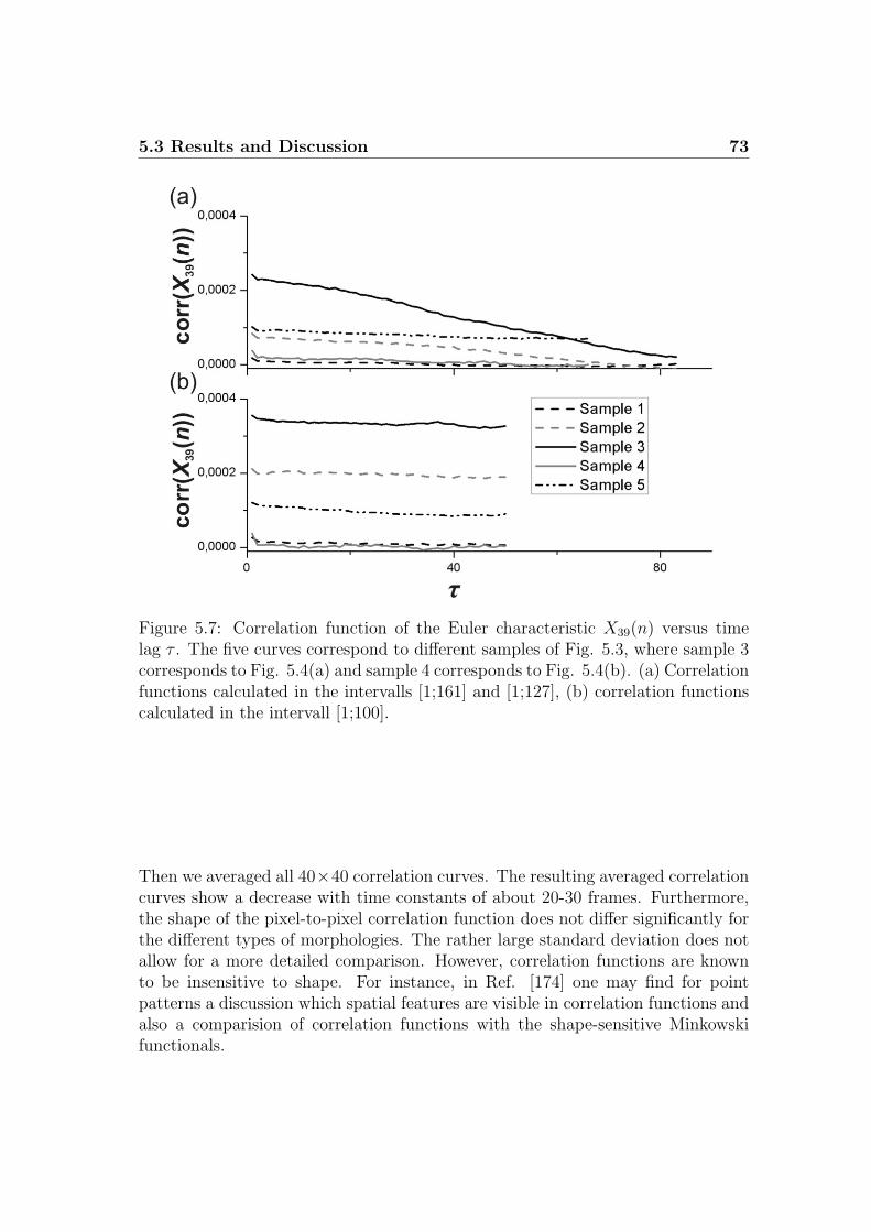
5.3 Results and Discussion 73
Figure 5.7: Correlation function of the Euler characteristic X39(n) versus timelag τ . The five curves correspond to different samples of Fig. 5.3, where sample 3corresponds to Fig. 5.4(a) and sample 4 corresponds to Fig. 5.4(b). (a) Correlationfunctions calculated in the intervalls [1;161] and [1;127], (b) correlation functionscalculated in the intervall [1;100].
Then we averaged all 40×40 correlation curves. The resulting averaged correlationcurves show a decrease with time constants of about 20-30 frames. Furthermore,the shape of the pixel-to-pixel correlation function does not differ significantly forthe different types of morphologies. The rather large standard deviation does notallow for a more detailed comparison. However, correlation functions are knownto be insensitive to shape. For instance, in Ref. [174] one may find for pointpatterns a discussion which spatial features are visible in correlation functions andalso a comparision of correlation functions with the shape-sensitive Minkowskifunctionals.

74 5. Characterization of block copolymer microdomain dynamics
Figure 5.8: Averaged pixel-to-pixel correlations of image samples P (x, y) (wherex and y are the spatial coordinates) versus time lag τ . The curves correspond tothe same samples as in Fig. 5.7. At three spots error bars indicating the standarddeviation of the correlation function corresponding to sample 3 are shown. Thestandard deviation is similar for all τ and for all samples.
5.3.2 Skeletonization
By skeletonizing and classifying the SPM images shown in Fig. 5.4(a) we yielda time series of two-dimensional graphs consisting of white lines and classifiedbranchings (Fig. 5.9). Figure 5.9(a) shows the graph corresponding to frame 1 inFig. 5.4(a), Fig. 5.9(b) corresponds to frame 70 (not shown in Fig. 5.4(a)) andFig. 5.9(c) corresponds to the last frame in 5.4(a). The details of the resultinggraph depend on the binarization method and on the image pre-processing. Toget a better comparison with the Minkowski method we also binarized the SPMimages with a fixed threshold ρ = 0.39.
Figure 5.10(a) shows the temporal evolution of the number of threefold branch-ings (y-connections) for sample 3 and 4 in Fig. 5.3. The shape of the curve appearsto be quite similar as the temporal evolution of the Euler characteristic shown inFig. 5.6. For sample 4 the number of threefold branchings is fluctuating around amore or less constant value (Fig. 5.10(a)).

5.3 Results and Discussion 75
Figure 5.9: Reduced skeleton of frame 1, 67, and 161 of the sequence of imagesshown in Fig. 5.4(a).
Figure 5.10: (a) Number of y-connections versus frame number n of sample 3 and4 corresponding to the data sets shown in Fig. 5.4(a) and Fig. 5.4(b), respectively.(b) Correlation function of the number of y-connections versus time lag τ . Sample 3and 4 correspond to the data sets shown in Fig. 5.4(a) and Fig. 5.4(b), respectively.For sample 3, also the correlation function for frame 1 to frame 100 is shown.
76 5. Characterization of block copolymer microdomain dynamics
For sample 3, however, it increases first slightly and starts to decrease at frame120. The morphological transition is also visible in the temporal evolution of y-connections. When the structure does not change the curve fluctuates arounda constant mean. Computing the correlation functions for the two curves (Fig.5.10(b)) a similar behavior can be seen as in Fig. 5.7. As the correlation curvecorresponding to sample 3 shows a slow decrease with a time constant of 40-50frames (Fig. 5.10(b)) the correlation curve belonging to sample 4 decreases veryfast indicating that no temporal correlations exist on the studied time scale.
5.4 Conclusion
We have demonstrated and compared three different approaches for quantifyingthe temporal evolution of the local morphology of the microdomain structure ofa thin film of block copolymer. Compared to other methods in the literature[14–17] local Minkowski functionals and statistics based on the skeletonizationof SPM gray scale images have the advantage to analyze the data in real space.In addition they do not depend on periodic patterns or statistical assumptions.Therefore, they are especially suited for morphologies containing a lot of defectswhose evolution should be tracked and whose temporal and lateral correlationsshould be investigated. Furthermore, Minkowski functionals computed as functionof the threshold value require no a priori model of the structure. However, thesecurves contain redundant information. Reducing them to characteristic valueswhich can be tracked over time must be done carefully. We have shown thatan intervall of thresholds can be idendified where different morphologies can bedistinguished in a robust way, which does not depend on the particular choice ofthe threshold value.
Our results show that Minkowski functionals are not only applicable to theanalysis of structure transitions in simulated data [79] but as well to the analysisof the more noisy data in SPM experiments. We analyzed the fluctuations of thetime dependent Euler characteristic and the temporal evolution of y-connectionsby correlation analysis. In both no characteristic time constants could be detectedin the fluctuations. On larger time scales the correlation functions are dominatedby structural transitions of the examined patterns. None of the three methodsshows a temporal correlation in the microdomain dynamics of the studied dataset. The presented methods appear as well suited tools for the search for possiblelateral correlations of defect dynamics, which is a topic of future work.

5.5 Acknowledgements 77
5.5 Acknowledgements
This work was supported by the VolkswagenStiftung and the European Comission(FORCETOOL, NMP4-CT-2004-013684). Furthermore, the authors would liketo thank Christian Franke for implementing the local Minkowski algorithm andMarcus Bohme for measuring the analyzed image sequence.

78 5. Characterization of block copolymer microdomain dynamics

Chapter 6
Summary
A curvature based non-linear registration algorithm for series of 2D images, whichwas originally developed for medical applications, has been adapted for the appli-cation to scanning probe microscopy (SPM) images. It has been expanded by animplicit mapping for the handling of image artifacts and boundaries. Furthermore,the quality and the speed of non-linear curvature registration has been improvedby processing the SPM images as a complete image block and by using a multi-resolution approach. In this way, the quality of 3D nanotomography data setsand of SPM movies has been improved significantly. Large areas of 1 µm × 1 µmcan now be tracked over long time spans or in 3D with a high resolution of up to10 nm. The method proved to be applicable to SPM images of a broad range ofmaterials such as block copolymers, semicrystalline polymers, metallic alloys, andhuman bone. 3D data sets which are obtained in this way give new insights intothe structure of materials which could not be investigated in such detail before.Additionally, the proper registration gives way for a better quantitative analy-sis. The combination of nanotomography with in-situ observations of dynamicalprocesses provides a deeper insight to structure formation mechanisms.
Since the view into 3D density distributions is often obstructed a new data re-duction and visualization technique for 3D block copolymer microdomain networkstructures has been introduced. First, the 3D skeleton of these structures has beencomputed. In a second pass the resulting network of thin lines has been adequatelysmoothed and corrected for artifacts. Then branching points have been classifiedand color coded. With the help of such classified graphs the temporal evolutionof block copolymer microdomain structures can be much easier perceived. Themethod has been applied to 3D simulation data as well as to 2D SPM moviesof the microdomain dynamics in thin films of cylinder forming block copolymers.The improved visualization simplifies a visual comparison of different simulationmethods as well as the comparison of theoretical predictions with experimentaldata. Moreover, the tracking of numbers of characteristic point defects with time

80 6. Summary
allows for a quantitative comparison. As an example, a series of SPM images dis-playing the structure formation in a thin film of polystyrene-block -polybutadienehas been quantified by this method.
In addition and for comparison, the same data has been analyzed with localMinkowski measures which are better suited for characterization of local struc-tures within gray scale images. These measures yield morphological and geomet-rical informations about the observed structure. The study of block copolymermicrodomains by local measures proved to be a useful extention of present meth-ods in the literature. By varying the local window size structure information atdifferent length scales can be acquired and compared. Correlation functions ofthe temporal evolution of Minkowski measures and branching points have beencomputed and compared with pixel-to-pixel correlation functions.
In summary, the image processing methods developed and demonstrated withinthis thesis have been proven to be an enhancement for SPM studies of variousmaterials. In particular, the image quality of volume images and movies hasbeen drastically improved, which allowed the observation of previously not visiblephysical phenomena. Using these methods important contributions to a betterunderstanding of these materials have been achieved. The methods presented inthis thesis are not limited to SPM data and promiss to facilitate further advanceson the study of micro- and nanoscaled materials.

List of Figures
1.1 Principle of nanotomography. (Adapted from [20]; c©2000 by theAmerican Physical Society). . . . . . . . . . . . . . . . . . . . . . . 11
1.2 Isosurface of a crystalline lamella in elastic polypropylene after rigidregistration and after curvature based registration. (Adapted from[21]; c©2006 by the Institute of Physics). . . . . . . . . . . . . . . . 12
1.3 Schematic illustration of the projection imaging process. (Adaptedfrom Ref. [55]; c©1999 by Academic Press). . . . . . . . . . . . . . . 13
1.4 Demonstration of different visualization techniques for 3D volumedata sets on the example of a 3D nanotomography image of poly-styrene-block -polybutadiene copolymer [43, 74]. . . . . . . . . . . . 14
1.5 Reduction of a gray scale SPM image to a 2D network graph. . . . 151.6 Examples of ±1
2disclinations and dislocations. (Adapted from [14];
c©2002 by the American Physical Society). . . . . . . . . . . . . . . 161.7 SPM height image of polystyrene-block -poly(2-vinylpyridine) and
corresponding Voronoi diagram. (Adapted from [16]; c©2003 by theAmerican Chemical Society). . . . . . . . . . . . . . . . . . . . . . . 16
2.1 Principle of nanotomography. (Adapted from [20]; c©2000 by theAmerican Physical Society). . . . . . . . . . . . . . . . . . . . . . . 20
2.2 Schematic description of the relative tip movement during an SPMmeasurement. . . . . . . . . . . . . . . . . . . . . . . . . . . . . . . 21
2.3 Tapping mode phase image of an etched surface of semicrystallinepolypropylene. . . . . . . . . . . . . . . . . . . . . . . . . . . . . . . 25
2.4 Tapping mode phase image with margin, nonlinear registered imageand corresponding deformation grid. . . . . . . . . . . . . . . . . . 25
2.5 Crystalline lamella in ePP after rigid registration and after curva-ture based registration. . . . . . . . . . . . . . . . . . . . . . . . . . 29
2.6 Nanotomography image of the crystalline regions of ePP (the samedata set is shown in Ref. [22] from another perspective.) . . . . . . 30
2.7 Cross section through an ePP film displaying the different orienta-tions of crystalline lamellae. . . . . . . . . . . . . . . . . . . . . . . 30

82 LIST OF FIGURES
2.8 Topographic image of the Ni3Al/Ni alloy CMSX 6. Comparison ofrigid and non-linear registration of a section of the 2D data set. . . 31
3.1 SPM phase images of ePP imaged at the same spot [74]. . . . . . . 34
3.2 Stack of 82 SPM phase images corresponding to Fig. 3.1 displayedby a cut in x-t direction. . . . . . . . . . . . . . . . . . . . . . . . . 35
3.3 Example of a deformation grid according to the non-linear registra-tion of the data shown partly in Fig. 3.1. . . . . . . . . . . . . . . . 35
3.4 Detail of a series of SPM phase images displaying the crystallizationprocess of one lamella. (From Ref. [25]; c©2007 by the AmericanChemical Society). . . . . . . . . . . . . . . . . . . . . . . . . . . . 36
3.5 Detail of a nanotomography image of crystallized ePP. (From Ref.[25]; c©2007 by the American Chemical Society). . . . . . . . . . . . 37
3.6 Schematics of a screw dislocation together with top views of sectionslabeled in the schematics. (From Ref. [25]; c©2007 by the AmericanChemical Society). . . . . . . . . . . . . . . . . . . . . . . . . . . . 37
3.7 Defect structure with moving polystyrene bead (From Ref. [24]). . . 39
3.8 Meandering cylinders of polystyrene (From Ref. [24]). . . . . . . . . 39
3.9 Stacked SPM phase images of the rearrangement dynamics of poly-styrene-block -polybutadiene microdomains (From Ref. [24]). . . . . 40
3.10 Isosurface of a 3D nanotomography image of polystyrene-block -poly-butadiene copolymer [43, 74]. . . . . . . . . . . . . . . . . . . . . . 41
3.11 Series of SPM images showing the transition from a disorderedstructure to a highly ordered stripe pattern. (From Ref. [103];c©2006 by the Royal Society of Chemistry). . . . . . . . . . . . . . 42
3.12 Detail of the SPM images shown in Fig. 3.11 displaying a groupof defects which dissolve to the end of the measurement almostcompletely. Additionally, the defect annihilation is shown by someschematics. (From Ref. [103]; c©2006 by the Royal Society of Chem-istry). . . . . . . . . . . . . . . . . . . . . . . . . . . . . . . . . . . 42
3.13 3D isosurface image of human bone etched with a 0.1 molar solutionof HCl. (From Ref. [23]; c©2007 by the American Institute ofPhysics). . . . . . . . . . . . . . . . . . . . . . . . . . . . . . . . . . 44
4.1 Comparison between different visualization techniques for 3D Meso-dyn simulation data sets. . . . . . . . . . . . . . . . . . . . . . . . . 47
4.2 Illustration of the data reduction and visualization technique. . . . 48
4.3 Reduced representation of the network of A-cylinders in a simu-lated thin film of A3B12A3 block copolymers, calculated from anisosurface with threshold value ρA = 0.33. . . . . . . . . . . . . . . 51
LIST OF FIGURES 83
4.4 Sequence of microdomain structures during the gyroid-to-cylindertransition observed in this work. The sequence is compared with asequence of structures during the cylinder-to-gyroid transition pre-dicted by Matsen [145]. (Adapted from Ref. [145]; c©1998 by theAmerican Physical Society). . . . . . . . . . . . . . . . . . . . . . . 53
4.5 Snapshots of movie 2 (see supplementary data [154]) showing thedynamics of the A-density in the plane defined by the thick blacklines shown in Fig. 4.3 and Fig. 4.4(a) . . . . . . . . . . . . . . . . 54
4.6 Example 1 (one voxel protrusion A) . . . . . . . . . . . . . . . . . . 58
4.7 Example 2 (one voxel protrusion B) . . . . . . . . . . . . . . . . . . 58
4.8 Example 3 (triangle) . . . . . . . . . . . . . . . . . . . . . . . . . . 59
4.9 Example 4 (triangle) . . . . . . . . . . . . . . . . . . . . . . . . . . 59
4.10 Example 5 (four point cluster) . . . . . . . . . . . . . . . . . . . . . 59
5.1 (a) TappingMode SPM phase image P (x, y) of a thin film of acylinder forming polystyrene-block -polybutadiene-block -polystyrenecopolymer. The sample is similar to that shown in Fig. 6(b) inRef. [147]. (b) Map of the corresponding local Euler characteris-tic X39(x, y) calculated with box size 14 × 14 pixels and thresholdρ = 0.39. . . . . . . . . . . . . . . . . . . . . . . . . . . . . . . . . . 66
5.2 Area A, Euler Characteristic X, perimeter P , and the ratio X/Pas function of the threshold ρ calculated for different samples withdifferent morphologies. . . . . . . . . . . . . . . . . . . . . . . . . . 68
5.3 SPM phase image of a polystyrene-block -polybutadiene copolymerswollen in chloroform vapor [26]. . . . . . . . . . . . . . . . . . . . . 69
5.4 Two samples (40× 40 pixels) of the film shown in Fig. 5.3 observedduring increasing saturation with chloroform vapor from 10 to 80%.The individual images show the dynamics of the film. . . . . . . . . 70
5.5 Gray scale maps of the Euler characteristic X at box size 40 × 40pixels as a function of density threshold ρ and frame number n. . . 71
5.6 Euler characteristic X39(n) and X33(n) for density threshold ρ = 39and ρ = 33, respectively, versus frame number n. . . . . . . . . . . . 72
5.7 Correlation function of the Euler characteristic X39(n) versus timelag τ . The five curves correspond to different samples of Fig. 5.3. . 73
5.8 Averaged pixel-to-pixel correlations of image samples P (x, y) versustime lag τ . The curves correspond to the same samples as in Fig.5.7. . . . . . . . . . . . . . . . . . . . . . . . . . . . . . . . . . . . . 74
5.9 Reduced skeleton of frame 1, 67, and 161 of the sequence of imagesshown in Fig. 5.4(a). . . . . . . . . . . . . . . . . . . . . . . . . . . 75

84 LIST OF FIGURES
5.10 (a) Number of y-connections versus frame number n of sample 3and 4 in Fig. 5.4. (b) Correlation function of the number of y-connections versus time lag τ . . . . . . . . . . . . . . . . . . . . . . 75

Bibliography
[1] J. K. Udupa, G. T. Herman (eds.), 3D Imaging in Medicine, CRC Press,Boca Raton, FL (2000).
[2] I. N. Bankman (ed.), Handbook of Medical Imaging: Processing and Analysis,Academic Press, San Diego, CA (2000).
[3] N. Bartelme, Geoinformatik: Modelle, Strukturen, Funktionen, Springer,Berlin, DE (2005).
[4] J. Wayman, A. K. Jain, D. Maltoni, Biometric Systems, Technology, Designand Performance Evaluation, Springer, London, UK (2005).
[5] B. Jahne, Practical Handbook on Image Processing for Scientific and Tech-nical Applications, CRC Press, Boca Raton, FL (2004).
[6] J. C. van den Berg (ed.), Wavelets in Physics, Cambridge University Press,Cambridge, UK (2004).
[7] K. R. Mecke, Additivity, Convexity, and Beyond: Applications of MinkowskiFunctionals in Statistical Physics, Lect. Not. Phys., Springer, Berlin, DE554, 111 (2000).
[8] K. R. Mecke and D. Stoyan (eds.), Morphology of Condensed Matter. Physicsand Geometry of Spatially Complex Systems, Lect. Not. Phys. 600, Springer,Berlin, DE (2002).
[9] G. Binnig, H. Rohrer, C. Gerber, and E. Weibel, Phys. Rev. Lett. 49, 57(1982).
[10] NanoScope Software 6.13, Veeco Instruments Inc., Santa Barbara, CA.
[11] Scanning Probe Image Processor 4.5.8, Image Metrology A/S, Hørsholm,DK.

86 BIBLIOGRAPHY
[12] D. Necas and P. Klapetek, Gwyddion, Czech Metrology Institute, Brno, CZ;http://www.gwyddion.net.
[13] WSxM 2.1, Nanotech Electronica S. L., Tres Cantos, ES.
[14] C. K. Harrison, Z. Cheng, S. Sethuraman, D. A. Huse, P. M. Chaikin, D. A.Vega, J. M. Sebastian, R. A. Register and D. H. Adamson, Phys. Rev. E 66,011706 (2002).
[15] C. K. Harrison, D. H. Adamson, Z. Cheng, J. M. Sebastian, S. Sethuraman,D. A. Huse, R. A. Register and P. M. Chaikin, Science 290, 1558 (2000).
[16] R. A. Segalman, A. Hexemer, R. C. Hayward, and E. J. Kramer, Macro-molecules 36, 3272 (2003).
[17] R. A. Segalman, A. Hexemer, and E. J. Kramer, Macromolecules 36, 6831(2003).
[18] R. Wiesendanger, Scanning Probe Microscopy and Spectroscopy, CambridgeUniversity Press, Cambridge, UK (1994).
[19] B. Fischer and J. Modersitzki, J. Math. Imaging Vis. 18, 81 (2003).
[20] R. Magerle, Phys. Rev. Lett. 85, 2749 (2000).
[21] S. Scherdel, S. Wirtz, N. Rehse, and R. Magerle, Nanotechnology 17, 881(2006).
[22] N. Rehse, S. Marr, S. Scherdel, and R. Magerle, Adv. Mater. 17, 2203 (2005).
[23] C. Dietz, S. Roper, S. Scherdel, A. Bernstein, N. Rehse, and R. Magerle,Rev. Sci. Instrum. 78, 053703 (2007).
[24] M. Kreis, Dynamik in dunnen Blockcopolymerfilmen, diploma thesis, Uni-versitat Bayreuth (2005).
[25] M. Franke and N. Rehse, Macromolecules (in print).
[26] M. Bohme, Defekt-Dynamik in dunnen Blockcopolymerfilmen, diploma the-sis, Technische Universitat Chemnitz, Chemnitz, DE (2007).
[27] S. Rehse, K. Mecke, and R. Magerle (submitted to Phys. Rev. E).
[28] M. Goken, R. Magerle, M. Hund, and K. Durst, Prakt. Metallogr. Sonderbd.35, Metallographietagung Berlin 2003 (ed. P.D. Portella) 257 (2004).

BIBLIOGRAPHY 87
[29] J. Frank (ed.), Electron Tomography, Plenum Press, New York, N. Y. (1992).
[30] M. Weyland and P. A. Midgley, Mater. Today 7, 32 (2004).
[31] R. C. Barrett and C. F. Quate, Rev. Sci. Instrum. 62, 1393 (1991).
[32] M. S. Hoogeman, D. G. Vanloon, R. W. M. Loos, H. G. Ficke, E. Dehaas,J. J. Vanderlinden, H. Zeijlemaker, L. Kuipers, M. F. Chang, M. A. J. Klik,and J. W. M. Frenken, Rev. Sci. Instrum. 69, 2072 (1998).
[33] D. Croft, S. Stilson, and S. Devasia, Nanotechnology 10, 201 (1999).
[34] S. Salapaka, A. Sebastian, J. P. Cleveland, and M. V. Salapaka, Rev. Sci.Instrum. 73, 3232 (2002).
[35] J. Kwon, J. Hong, Y. S. Kim, D. Y. Lee, K. Lee, S. Lee, and S. Park, Rev.Sci. Instrum. 74, 4378 (2003).
[36] Q. Zou and S. Devasia, IEEE Transactions on Control Systems Technology12, 375 (2004).
[37] M. Abe, Y. Sugimoto, O. Custance, and S. Morita, Appl. Phys. Lett. 87,173503 (2005).
[38] K. Henriksen and S. L. S. Stipp, Am. Mineral. 87, 5 (2002).
[39] J. Garnaes, L. Nielsen, K. Dirscherl, J. F. Jørgensen, J. B. Rasmussen, P. E.Lindelof, and C. B. Sørensen, Appl. Phys. A 66, 831 (1998).
[40] J. B. A. Maintz and M. A. Viergever, Med. Image Anal. 2, 1 (1998).
[41] A. G. Brown, ACM Comput. Surv. 24, 326 (1992).
[42] J. Modersitzki, Numerical methods for image registration, Oxford UniversityPress, Oxford, UK (2004).
[43] E.-C. Spitzner, personal communication.
[44] M. Uchic, L. Holzer, B. J. Inkson, E. L. Principe, and P. Munroe, MRSBulletin 32, 408 (2007).
[45] A. E. Efimov, A. G. Tonevitsky, M. Dittrich, and N. B. Matsko, J. Microsc.226, 207 (2007).
[46] F. S. Sjostrand, J. Ultrastruct. Res. 2, 122 (1958).

88 BIBLIOGRAPHY
[47] J. Radon, Ber. Verh. K. Sachs. Ges. Wiss. Leipzig, Math.-Phys. Kl. 69, 262(1917).
[48] D. J. DeRosier and A. Klug, Nature 217, 130 (1968).
[49] H. Stark, J. W. Woods, I. Paul, and R. Hingorani, IEEE Trans. ASSP 29,237 (1981).
[50] M. Radermacher, J. Electron Microsc. Tech. 9, 359 (1988).
[51] A. C. Kak and M. Slaney, Principles of Computerized Tomographic Imaging,IEEE Press, New York, N. Y. (1988).
[52] P. A. Midgley and M. Weyland, Ultramicroscopy 96, 413 (2003).
[53] R. Gordon, R. Bender, and G. T. Herman, J. Theor. Biol. 29, 471 (1970).
[54] P. Gilbert, J. Theor. Biol. 36, 105 (1972).
[55] B. F. McEwen and M. Marko, Methods in Cell Biology: Mitosis and Meiosis(ed. C. L. Rieder), Academic Press, Burlington, MA 61, 81 (1999).
[56] R. G. Hart, Science 159, 1464 (1068).
[57] B. F. McEwen and M. Marko, J. Histo-chem. Cytochem. 49, 553 (2001).
[58] H. Jinnai, Y. Nishikawa, R. J. Spontak, S. D. Smith, D. A. Agard, and T.Hashimoto, Phys. Rev. Lett. 84, 518 (2000).
[59] K. Yamauchi, K. Takahashi, H. Hasegawa, H. Iatrou, N. Hadjichristidis, T.Kaneko, Y. Nishikawa, H. Jinnai, T. Matsui, H. Nishioka, M. Shimizu, andH. Furukawa, Macromolecules 36, 6962 (2003).
[60] H. Sugimori, T. Nishi, and H. Jinnai, Macromolecules 38, 10226 (2005).
[61] T. Xu, A. V. Zvelindovsky, G. J. A. Sevink, K. S. Lyakhova, H. Jinnai, andT. P. Russell, Macromolecules 38, 10788 (2005).
[62] T. Kaneko, K. Suda, K. Satoh, M. Kamigaito, T. Kato, T. Ono, E. Naka-mura, T. Nishi, and H. Jinnai, Macromol. Symp. 242, 80 (2006).
[63] N. Kawase, M. Kato, H. Nishioka, and H. Jinnai, Ultramicroscopy 107, 8(2007).
[64] T. Ikehara, H. Jinnai, T. Kaneko, H. Nishioka, and T. Nishi, J. Polym. Sci.:Part B: Polymer Physics 45, 1122 (2007).

BIBLIOGRAPHY 89
[65] W. A. Kalender, Phys. Med. Biol. 51, R29 (2006).
[66] O. Brunke, D. Neuber, and D. K. Lehmann, Mater. Res. Soc. Symp. Proc.990, 0990-B05-09 (2007).
[67] I. W. Hamley, The Physics of Block Copolymers, Oxford University Press,Oxford, UK (1998).
[68] C. Park, J. Yoon, and E. L. Thomas, Polymer 44, 6725 (2003).
[69] see, e.g., Fig. 10 in Ref. [61]; Figs. 6 and 7 in Ref. [134]; Figs. 3, 6, 9, and 11in Ref. [135].
[70] see, e.g., Figs. 1, 3, and 4 in Ref. [133].
[71] D. Hoffman, Nature (London) 384, 28 (1996).
[72] see, e.g., Figs. 16, 17, and 18 in M. E. Vigild, K. Almdal, K. Mortensen, I.W. Hamley, J. P. A. Fairclough, and A. J. Ryan, Macromolecules 31, 5702(1998).
[73] G. E. Schroder-Turk, A. Fogden, and S. T. Hyde, Europ. Phys. J. B 54, 509(2007).
[74] C. Dietz, personal communication.
[75] A. Horvat, K. S. Lyakhova, G. J. A. Sevink, A. V. Zvelindowvsky, and R.Magerle, J. Chem. Phys. 120, 1117 (2004).
[76] A. Okabe, B. Boots, K. Sugihara, S. N. Chiu, Spatial Tessellations: Conceptsand Applications of Voronoi Diagrams, John Wiley & Sons, Chichester, UK(2000).
[77] D. A. Vega, C. K. Harrison, D. E. Angelescu, M. L. Trawick, D. A. Huse, P.M. Chaikin, and R. A. Register, Phys. Rev. E 71, 061803 (2005).
[78] P. Soille, Morphological Image Analysis, Springer, Berlin (2003).
[79] G. J. A. Sevink and A. V. Zvelindovsky, J. Chem. Phys. 121, 3864 (2004).
[80] M. Pinna, A. V. Zvelindovsky, S. Todd, and G. Goldbeck-Wood, J. Chem.Phys. 125, 154905-1 (2006).
[81] G. J. A. Sevink, Nanostructured Soft Matter: Experiments, theory & per-spectives (Ed. A. V. Zvelindovsky), Springer (2007).

90 BIBLIOGRAPHY
[82] K. R. Mecke, Int. J. Modern Phys. B 12, 861 (1998).
[83] K. R. Mecke, Phys. Rev. E 53, 4794 (1996).
[84] K. Jacobs, R. Seemann, and K. Mecke, Dynamics of Dewetting and StructureFormation in Thin Liquid Films in Lect. Not. Phys., Springer, Berlin, DE554, 72 (2000).
[85] K. Michielsen, H. De Raedt, and J. G. E. M. Fraaije, Prog. Theor. Phys.Suppl. 138, 543 (2000).
[86] A. Aksimentiev, K. Moorthi, and R. Holyst, J. Chem. Phys. 112, 6049 (2000).
[87] M. Konrad, A. Knoll, G. Krausch, and R. Magerle, Macromolecules 33, 5518(2000).
[88] S. N. Magonov and M.-H. Whangbo, Surface Analysis with STM and AFM,VCH Publishers, Weinheim, DE (1996).
[89] A. Knoll, K. S. Lyakhova, A. Horvat, G. Krausch, G. J. A. Sevink, A. V.Zvelindovsky, and R. Magerle, Nat. Mat. 3, 886 (2004).
[90] S. Scherdel, S. Wirtz, N. Rehse, and R. Magerle, Proc. of 10th Int. Fall Work-shop - Vision, Modeling, and Visualization (eds. G. Greiner, J. Hornegger,H. Niemann, and M. Stamminger), Akademische Verlagsgesellschaft, Berlin,DE 87 (2005).
[91] R. Garcıa and A. San Paulo, Phys. Rev. B 61, R13381 (2000).
[92] A. San Paulo and R. Garcıa, Phys. Rev. B 66, R041406 (2002).
[93] S. Wirtz, B. Fischer, J. Modersitzki, and O. Schmitt, Proc. of the SPIE 2004(eds. J. M. Fitzpatrick and M. Sonka), SPIE Press, 5370, 328 (2004).
[94] P. J. Burt and E. H. Adelson, IEEE T. Commun. 31, 532 (1983).
[95] H. Nyquist, Trans. AIEE 47, 617 (1928).
[96] W. Joo, M. S. Park, and J. K. Kim, Langmuir 22, 7960 (2006).
[97] T. Thurn-Albrecht, J. Schotter, G. A. Kastle, N. Emley, T. P. Russell, M. T.Tuominen, T. Shibauchi, L. Krusin-Elbaum, and C.T. Black, Science 290,2126 (2000).
[98] M. Kreis, personal communication.

BIBLIOGRAPHY 91
[99] A. Knoll, A. Horvat, K. S. Lyakhova, G. Krausch, G. J. A. Sevink, A. V.Zvelindovsky, and R. Magerle, Phys. Rev. Lett. 89, 035501 (2002).
[100] K. Amundson, E. Helfand, D. D. Davis, X. Quan, S. S. Patel, and S. D.Smith, Macromolecules 24, 6546 (1991).
[101] T. Thurn-Albrecht, J. DeRouchy, T. P. Russell, and H. M. Jager, Macro-molecules 33, 3250 (2000).
[102] A. Boker, A. Knoll, H. Elbs, V. Abetz, A. H. E. Muller, and G. Krausch,Macromolecules 35, 1319 (2002).
[103] V. Olszowka, M. Hund, V. Kuntermann, S. Scherdel, L. Tsarkova, A. Boker,and G. Krausch, Soft Matter 2, 1089 (2006).
[104] K. I. Winey, S. S. Patel, R. G. Larson, and H. Watanabe, Macromolecules26, 4373 (1993).
[105] G. Schmidt, W. Richtering, P. Lindner, and P. Alexandridis, Macromolecules31, 2293 (1998).
[106] J. Bodycomb, Y. Funaki, K. Kimishima, and T. Hashimoto, Macromolecules32, 2075 (1999).
[107] M. Hund and H. Herold, German Patent, No. DE102004043191 B4, Germany(2005).
[108] G. Holden, R. P. Quirck, and H. R. Kricheldorf, Thermoplastic Elastomers,Carl Hanser Verlag, Munchen, DE (2004).
[109] G. Reiter and J.-U. Sommer (eds.), Polymer Crystallisation: Observations,Concepts, and Illustrations, Lect. Not. Phys. 606, Springer, Berlin, DE(2003).
[110] H. Schonherr, R. M. Waymouth, and C. W. Frank, Macromolecules 36, 2412(2003).
[111] G. Hauser, J. Schmidtke, G. Strobl, and T. Thurn-Albrecht, ACS SymposiaSeries 739, 140 (2000).
[112] A. Gradys, P. Sajkiewicz, A. A. Minakov, S. Adamovsky, C. Schick, and T.Hashimoto, Mat. Sci. Eng. A 413-414, 442 (2005).
[113] D. C. Basset, Phil. Trans. R. Soc. Lond. A 348, 29 (1994).

92 BIBLIOGRAPHY
[114] D. Baumhoer, I. Steinbruck, and W. Goz, Histologie: Kurzlehrbuch mitSchemazeichnung, Urban and Fischer, Munchen, DE (2000).
[115] H. D. Wagner and S. Weiner, Ann. Rev. Mat. Sci. 28, 271 (1998).
[116] W. J. Landis, K. J. Hodgens, J. Arena, M. J. Song, and B. F. McEwen,Microsc. Res. Tech. 33, 192 (1996).
[117] H. Gao, B. Ji, I. L. Jager, E. Arzt, and P. Fratzl, Proc. Nat. Acad. Sci.(USA) 100, 5597 (2003).
[118] K. Tai, H. J. Qi, and C. Ortiz, J. Mat. Sci.: Mat. in Medicine 16, 947 (2005).
[119] H. S. Gupta, W. Wagermaier, G. A. Zickler, D. Raz-Ben Aroush, S. S. Funari,P. Roschger, H. D. Wagner, and P. Fratzl, Nano Lett. 5, 2520 (2005).
[120] H. S. Gupta, J. Seto, W. Wagermaier, P. Zaslansky, P. Boesecke, and P.Fratzl, Proc. Nat. Acad. Sci. (USA) 103, 17741 (2006).
[121] S. Roper, Nanotomographie an Biomaterialien, diploma thesis, TechnischeUniversitat Chemnitz, Chemnitz, DE (2006).
[122] S. Roper, personal communication.
[123] C. Riesch, Analyse von SPM-Bilddaten mittels Gabortransformation, B. S.thesis, Technische Universitat Chemnitz (2007).
[124] S.-S. Sun and N. S. Sariciftci (eds.), Organic Photovoltaics: Mechanisms,Materials, and Devices, CRC Press, Boca Raton, FL (2005).
[125] K. Mullen, U. Scherf (eds.), Organic Light Emitting Devices: Synthesis,Properties and Applications, Wiley-VCH Verlag, Weinheim (2006).
[126] S. Iijima, Nature 354, 56 (1991).
[127] N. Rehse, personal communication.
[128] M. Franke, personal communication.
[129] S. Scherdel, H. G. Schoberth, and R. Magerle, J. Chem. Phys. 127, 014903(2007).
[130] K. Katsov, M. Muller, and M. Schick, Biophys. J. 87, 3277 (2004); 90, 915(2006).
[131] S. Hyde, S. Andersson, K. Larsson, Z. Blum, T. Landh, S. Lidin, and B. W.Ninham, The Language of Shape, Elsevier Science, Amsterdam (1997).
BIBLIOGRAPHY 93
[132] For a review, see, G. H. Fredrickson, V. Ganesan, and F. Drolet, Macro-molecules 25, 16 (2002).
[133] A. V. Zvelindovsky, G. J. A. Sevink, B. A. C. van Vlimmeren, N. M. Maurits,and J. G. E. M. Fraaije, Phys. Rev. E 57, R4879 (1998).
[134] A. V. Zvelindovsky and G. J. A. Sevink, Europhys. Lett. 62, 370 (2003).
[135] A. V. Zvelindovsky, G. J. A. Sevink, and J. G. E. M. Fraaije, Phys. Rev. E62, R3063 (2000).
[136] B. Lichtenbelt, R. Crane, and S. Naqvi, Introduction to Volume Rendering,Prentice-Hall PTR, Upper Saddle River, NJ (1998).
[137] L. Tsarkova, A. Horvat, G. Krausch, A. V. Zvelindovsky, G. J. A. Sevink,and R. Magerle, Langmuir 22, 8089 (2006).
[138] K. S. Lyakhova, A. Horvat, A. V. Zvelindovsky, and G. J. A. Sevink, Lang-muir 22, 5848 (2006).
[139] T. Xu, A. V. Zvelindovsky, G. J. A. Sevink, O. Gang, B. Ocko, Y. Zhu, S.P. Gido, and T. P. Russell, Macromolecules 37, 6980 (2004).
[140] I. W. Hamley, V. Castelletto, O. O. Mykhaylyk, and Z. Yang, Langmuir 20,10785 (2004).
[141] K. Schmidt, A. Boker, H. Zettl, F. Schubert, H. Hansel, F. Fischer, T. M.Weiss, V. Abetz, A. V. Zvelindovsky, G. J. A. Sevink, and G. Krausch,Langmuir 21, 11974 (2005).
[142] K. S. Lyakhova, A. V. Zvelindovsky, and G. J. A. Sevink, Macromolecules39, 3024 (2006).
[143] K. Schmidt, H. G. Schoberth, F. Schubert, H. Hansel, F. Fischer, T. M.Weiss, G. J. A. Sevink, A. V. Zvelindovsky, A. Boker, and G. Krausch, SoftMatter 3, 448 (2007).
[144] A. V. Kyrylyuk, A. V. Zvelindovsky, G. J. A. Sevink, and J. G. E. M. Fraaije,Macromolecules 35, 1473 (2002); A. V. Zvelindovsky, and G. J. A. Sevink,Phys. Rev. Lett. 90, 049601 (2003).
[145] M. W. Matsen, Phys. Rev. Lett. 80, 4470 (1998).
94 BIBLIOGRAPHY
[146] J. G. E. M. Fraaije, J. Chem. Phys. 99, 9202 (1993); J. G. E. M. Fraaije, B.A. C. van Vlimmeren, N. M. Maurits, M. Postma, O. A. Evers, C. Hoffmann,P. Altevogt, and G. Goldbeck-Wood, J. Chem. Phys. 106, 4260 (1997); G.J. A. Sevink, A. V. Zvelindovsky, B. A. C. van Vlimmeren, N. M. Maurits,and J. G. E. M. Fraaije, J. Chem. Phys. 110, 2250 (1999).
[147] A. Knoll, R. Magerle, and G. Krausch, J. Chem. Phys. 120, 1105 (2004).
[148] K. S. Lyakhova, A. Horvat, R. Magerle, G. J. A. Sevink, and A. V. Zvelin-dovsky, J. Chem. Phys. 120, 1127 (2004).
[149] L. Lam, S.-W. Lee, and C. Y. Suen, IEEE Trans. Pattern Anal. Mach. Intell.14, 869 (1992).
[150] M. W. Jones, J. A. Bærentzen, and M. Sramek, IEEE Transactions on Vi-sualization and Computer Graphics 12, 581 (2006).
[151] T. Grigorishin, G. Abdel-Hamid, and Y.-H. Yang, Pattern Analysis andApplications 1, 163 (1998).
[152] Y. F. Tsao and K. S. Fu, Comput. Graph. and Image Process. 17, 315 (1981).
[153] F. C. Bernstein, T. F. Koetzle, G. J. B. Williams, E. F. Meyer, Jr., M. D.Brice, J. R. Rodgers, O. Kennard, T. Shimanouchi, and M. Tasumi, J. Mol.Biol. 112, 535 (1977); H. M. Berman, J. Westbrook, Z. Feng, G. Gilliland,T. N. Bhat, H. Weissig, I. N. Shindyalov, and P. E. Bourne, Nucleic AcidsRes. 28, 235 (2000); http://www.pdb.org/.
[154] see section 4.7 and the CD which is enclosed in this thesis.
[155] W. L. DeLano, Pymol, DeLano Scientific, San Carlos, CA (2002);http://www.pymol.org.
[156] G. J. A. Sevink and A. V. Zvelindovsky, J. Chem. Phys. 121, 3864 (2004).
[157] L. Tsarkova, A. Knoll, and R. Magerle, Nano Lett. 6, 1574 (2006).
[158] D. A. Hayduk, S. M. Gruner, P. Rangarajan, R. A. Register, L. J. Fetters, C.Honeker, R. J. Albalak, and E. L. Thomas, Macromolecules 27, 490 (1994).
[159] S. Sakurai, T. Hashimoto, and L. J. Fetters, Macromolecules 29, 740 (1996).
[160] K. Kimishima, T. Koga, and T. Hashimoto, Macromolecules 33, 968 (2000).
[161] M. W. Matsen, J. Chem. Phys. 114, 8165 (2001).

BIBLIOGRAPHY 95
[162] C.-Y. Wang and T. P. Lodge, Macromolecules 35, 6997 (2002).
[163] J. Hahm, W. A. Lopes, H. M. Jaeger, and S. J. Sibener, J. Chem. Phys.109, 10111 (1998).
[164] J. Hahm and S. J. Siebener, J. Chem. Phys. 114, 4730 (2001).
[165] A. V. Zvelindovsky and G. J. A. Sevink, Europhys. Lett. 62, 370 (2003).
[166] P. K. Hansma, G. Schitter, G. E. Fantner, and C. Prater, Science 314, 601(2006).
[167] A. Rosenfeld and A. C. Kak, Digital Picture Processing, Academic Press,New York, N. Y. (1976).
[168] J. Serra, Image Analysis and Mathematical Morphology, Academic Press,New York, N. Y. (1982).
[169] L. A. Santalo, Integral Geometry and Geometric Probability, Addison-Wesley,Reading, MA (1976).
[170] J. Becker, G. Grun, R. Seemann, H. Mantz, K. Jacobs, K. Mecke, and R.Blossey, Nat. Mat. 2, 59 (2003); R. Fetzer, M. Rauscher, R. Seemann, K.Jacobs, and K. Mecke, Phys. Rev. Lett. 99, 114503 (2007).
[171] C. H. Arns, M. A. Knackstedt, W. V. Pinczewski, and K. R. Mecke, Phys.Rev. E 63, 031112 (2001); C. H. Arns, M. A. Knackstedt, and K. Mecke,Phys. Rev. Lett. 91, 215506 (2003).
[172] H. Hadwiger, Vorlesungen uber Inhalt, Oberflache und Isoperimetrie,Springer, Berlin, DE (1957).
[173] see also Ref. [78], page 340.
[174] K. Mecke and D. Stoyan, Biometrical Journal 47, 1 (2005).

96 BIBLIOGRAPHY

Selbstandigkeitserklarung nach §6Promotionsordnung
Ich erklare, dass ich die vorliegende Arbeit selbststandig und nur unter Verwendungder angegebenen Literatur und Hilfsmittel angefertigt habe. Ich erklare, nicht be-reits fruher oder gleichzeitig bei anderen Hochschulen oder an dieser Universitat einPromotionsverfahren beantragt zu haben. Ich erklare, obige Angaben wahrheits-gemaß gemacht zu haben und erkenne die Promotionsordnung der Fakultat furNaturwissenschaften der Technischen Universitat Chemnitz vom 10. Oktober 2001an.
Chemnitz, 23.11.2007
(Sabine Rehse)

Curriculum Vitae
Personliche Daten
Name Sabine RehseGeburtsdatum 30.10.1977Geburtsort BayreuthFamilienstand verheiratetGeburtsname ScherdelNationality deutsch
Schulausbildung
1988-1997 Wirtschaftswissenschaftliches Gymnasium, Bayreuth27.06.1997 Abschluss: Abitur
Wissenschaftliche Ausbildung
10/1997-04/2003 Mathematikstudium, Universitat Bayreuth, Bayreuth25.04.2003 Abschluss: Diplom-Mathematikerin05/2002-04/2003 Diplomarbeit Numerische Simulation von
Schmelzkarbonat-Brennstoffzellen: 1-D-PDAE-Modelle,ihr MOL-Index und ihre numerische DiskretisierungLehrstuhl Ingenieurmathematik, Universitat Bayreuth,Bayreuth
05/2003-01/2005 Doktorarbeit, Lehrstuhl Physikalische Chemie II,Universitat Bayreuth, Bayreuth,Nachwuchsgruppe von PD Dr. R. MagerleHigh Resolution Volume Imaging and Characterizationof Polymeric Materials with Nanotomography
02/2005-11/2007 Doktorarbeit, Chemische Physik, Technische UniversitatChemnitz, Chemnitz
Fremdsprachen
Englisch, Franzosisch


Publications
Publications in journals
The following publications are enclosed in this thesis (due to my marriage in 2007my name changed from Sabine Scherdel to Sabine Rehse):
• S. Scherdel, S. Wirtz, N. Rehse, and R. Magerle, Non-linear registration ofscanning probe microscopy images, Nanotechnology 17, 881 (2006).
• S. Scherdel, H. G. Schoberth, and R. Magerle, Visualizing the dynamics ofcomplex spatial networks in structured fluids, J. Chem. Phys. 127, 014903(2007).
• S. Rehse, K. Mecke, and R. Magerle, Characterization of the dynamics ofblock copolymer microdomains with local morphological measures (submit-ted).
Within the scope of my diploma and my PhD thesis the following publicationshave been additionally published:
• H. J. Pesch, K. Chudej, V. Petzet, S. Scherdel, K. Schittkowski, P. Heide-brecht, and K. Sundmacher, Numerical simulation of a 1D model of a moltencarbonate fuel cell, Proc. Appl. Math. Mech. 3, 521 (2003).
• K. Chudej, V. Petzet, S. Scherdel, H. J. Pesch, Kl. Schittkowski, P. Hei-debrecht, and K. Sundmacher, Index analysis of a nonlinear PDAE systemdescribing a molten carbonate fuel cell, Proc. Appl. Math. Mech. 3, 563(2003).
• K. Chudej, P. Heidebrecht, V. Petzet, S. Scherdel, K. Schittkowski, H. J.Pesch, and K. Sundmacher, Index analysis and numerical solution of a largescale nonlinear PDAE system describing the dynamical behaviour of moltencarbonate fuel cells, Z. Angew. Math. Mech. 85, 132 (2005).

• N. Rehse, S. Marr, S. Scherdel, and R. Magerle, Three-dimensional imagingof semicrystalline polypropylene with 10 nm resolution, Adv. Mater. 17,2203 (2005).
• S. Scherdel, S. Wirtz, N. Rehse, and R. Magerle, Non-linear registration ofscanning probe microscopy images, Proc. of 10th Int. Fall Workshop - Vision,Modeling, and Visualization (eds. G. Greiner, J. Hornegger, H. Niemann,and M. Stamminger), Akademische Verlagsgesellschaft, Berlin, 87 (2005).
• V. Olszowka, M. Hund, V. Kuntermann, S. Scherdel, L. Tsarkova, A. Boker,and G. Krausch, Large scale alignment of a lamellar block copolymer thin filmvia electric fields: a time-resolved SFM study, Soft Matter 2, 1089 (2006).
• C. Dietz, S. Roper, S. Scherdel, A. Bernstein, N. Rehse, and R. Magerle,Automatization of nanotomography, Rev. Sci. Instr. 78, 053703 (2007).
Presentations at international conferences
• Fruhjahrstagung der Deutschen Physikalischen Gesellschaft, Regensburg, 2004,Charakterisierung der Strukturbildung in Blockcopolymeren mit Minkowski-funktionalen (poster presentation).
• Jahrestagung der Gesellschaft fur Angewandte Mathematik und Mechanike.V., Dresden, 2004, Charakterisierung der Strukturbildung in Blockcopoly-meren mit Hilfe von Minkowskimaßen (oral presentation).
• Fruhjahrstagung der Deutschen Physikalischen Gesellschaft, Berlin, 2005,Non-linear registration of series of atomic force microscopy images of nanos-tructured materials (poster presentation).
• 10th International Fall Workshop: Vision, Modeling, and Visualization, Er-langen, 2005, Curvature registration of scanning probe microscopy images fornanotomography (poster presentation).
• WE-Heraeus-Seminar: Interplay of Thermodynamics and Hydrodynamics inCondensed Matter, Bad Honnef, 2006, Monitoring defect dynamics (posterpresentation).
• Fruhjahrstagung der Deutschen Physikalischen Gesellschaft, Dresden, 2006,Monitoring defect dynamics by local Minkowski measures (poster presenta-tion).

• Fruhjahrstagung der Deutschen Physikalischen Gesellschaft, Regensburg, 2007,Analysis of the microdomain dynamics in thin films of block copolymer (posterpresentation).

Acknowledgement - Danksagung
Zum Abschluß der Arbeit mochte ich mich bei einigen Leuten bedanken, die michbeim Erstellen dieser Arbeit unterstutzt haben.
• Ich danke Robert Magerle fur die Moglichkeit, diese Arbeit in seiner Gruppeanzufertigen, die erfolgreiche Zusammenarbeit und die fruchtbaren Diskus-sionen.
• Bei Klaus Mecke bedanke ich mich fur die vielen Diskussionen und diefreundliche Unterstutzung bei den Minkowskifunktionalen.
• Stefan Wirtz, Bernd Fischer und Jan Modersitzki mochte ich fur die Einfuhrungin die Registrierung und die gute Zusammenarbeit vor allem zu Beginnmeiner Doktorarbeit danken.
• Andriana Horvath gilt mein Dank fur die Zusammenarbeit bei der Analysevon Simulationsdaten mit Minkowskifunktionalen.
• Bei Markus Hund, Michael Scheurer, Heiko Schoberth und Christian Frankebedanke ich mich fur die Mithilfe und Unterstutzung beim Programmieren.
• Markus Hund, Sabine Marr, Violetta Olszowka, Martin Kreis, Markus Bohme,Mechthild Franke, Steffi Roper, Christian Dietz und Christian-Eike Spitznerdanke ich fur die großzugige Uberlassung von Messergebnissen.
• Fur seine Geduld bei meinen AFM-Messungsversuchen schulde ich ChristianDietz meinen Dank. Außerdem danke ich ihm und Maik Vieluf fur die lusti-gen Stunden, die wir bei der Erstellung des (kurzzeitig) kleinsten Fußballfeldsder Welt verbracht haben.
• Nico Rehse, Steffi Roper, Mechthild Franke, Christian Dietz, ChristianRiesch und Christian-Eike Spitzner mochte ich fur das Korrekturlesen voneinzelnen Kapiteln dieser Arbeit danken.
• Bei allen Mitarbeitern der PC II in Bayreuth und Chemische Physik in Chem-nitz bedanke ich mich fur die nette und produktive Arbeitsatmosphare.

• Zu guter Letzt gilt mein Dank Nico Rehse fur viele Diskussionen, seinechemische Sicht der Dinge und seine stets positive Einstellung (”Alles wirdgut”).