regularization in tomographypcha/talks/regtomo.pdf · regularization in tomography dealing with...

Regularization in Tomography Dealing with Ambiguity and Noise Per Christian Hansen Technical University of Denmark

May 2014 2/33 P. C. Hanaen: Regularization in Tomography

About Me …

• Professor of Scientific Computing at DTU • Interests: inverse problems, tomography, regularization algorithms, matrix compu-

tations, image deblurring, signal processing, Matlab software, … • Head of the project High-Definition Tomography,

funded by an ERC Advanced Research Grant. • Author of several Matlab software packages. • Author of four books.


Tomographic Reconstructions are Amazing!

Tomographic reconstructions are routinely computed each day. Our reconstruction algorithms are so reliable that we sometimes forget we are actually dealing with inverse problems with inherent stability problems.

This talk is intended for scientists who need a “brush up” on the underlying mathematics of some common tomographic reconstruction algorithms.

These algorithms are successful because they automatically incorporate regularization techniques that, in most cases, handle very well the stability issues.


Outline of Talk

We take a basic look at the inverse problem of “plain vanilla” absorption CT reconstruction and the associated stability problems:

• solutions are very sensitive to data errors, • solutions may fail to be unique.

We demonstrate how regularization is used to avoid these problems: • We make the reconstruction process stable by • incorporate regularization in reconstruction algorithm.

Webster Reg·u·lar·ize – to make regular by conformance to law, rules, or custom. Reg·u·lar – constituted, conducted, scheduled, or done in conformity with established or prescribed usages, rules, or discipline.

In tomography: we make the problem, or the solution, more regular in order to prevent it from being dominated by noise and other artefacts.

We look at the principles of different regularization techniques and show that they have different impact in the computed reconstructions.


The Origin of Tomography

Johan Radon, Über die Bestimmung von Funktionen durch ihre Integralwerte Längs gewisser Mannings-faltigkeiten, Berichte Sächsische Akadamie der Wis- senschaften, Leipzig, Math.-Phys. Kl., 69, pp. 262-277, 1917.

Main result: An object can be perfectly reconstructed from a full set of projections.

NOBELFÖRSAMLINGEN KAROLINSKA INSTITUTET

THE NOBEL ASSEMBLY AT THE KAROLINSKA INSTITUTE

11 October 1979

The Nobel Assembly of Karolinska Institutet has decided today to award the Nobel Prize in Physiology or Medicine for 1979 jointly to

Allan M Cormack and Godfrey Newbold Hounsfield

for the "development of computer assisted tomography".


The Radon Transform

The principle in parallel- beam tomography: send parallel rays through the object at different angles, measure the damping.

f(x) = 2D object / image, x =

·x1

x2

¸

f̂(Á; s) = sinogram / Radon transform

Line integral along line de¯ned by Á and s:

f̂(Á; s) =

Z 1

¡1f

µs

·cos Ásin Á

¸+ ¿

·¡ sin Ácos Á

¸¶d¿


The Inverse Radon Transform

Let R denote the Radon transform, such that

f̂ = R f , f = R¡1f̂

How to conveniently write the inverse Radon transform:

R¡1 = c (¡¢)1=2R¤; c = constant

R¤ = backprojection (dual transform)

¢ = @2=@x21 + @2=@x2

2 = Laplacian

(¡¢)1=2 = high-pass ¯lter F³(¡¢)1=2»

´(!) = j!jF(»)(!)

The operators (¡¢)1=2 and R¤ commute { this leads to the¯ltered back projection (FBP) algorithm:

R¡1 = c R¤(¡¢)1=2 ! f = R¡1f̂ = c R¤(¡¢)1=2f̂ :

Not precisely how we com-

pute it.


Matlab Check …


“Naïve” FBP is Very Sensitive to Noise

The high-pass filter |ω| in ”naive” FBP amplifies high-frequency noise in data.

The solution is to insert an additional filter than dampens higher frequencies: |ω| → ψ(ω) · |ω|

1. Only |ω|

2. sinc filter (”Shepp-Logan”)

3. cos filter

4. Hamming filter

This is regularization!


FBP + Low-Pass Filter Suppresses Noise

180 projections

1000 projections More data is better! But we loose some details due to the filter (low-pass = smoothing).


FBP with Few Projections

Projection angles 10:10:100

Less data creates trouble!

Now the problem is underdetermined and artifacts appear.

Projection angles 15:15:180


Setting Up an Algebraic Model

Damping of i-th X-ray through domain: bi =

Rrayi

Â(s) d`; Â(s) = attenuation coef.

This leads to a large linear system:

A x = b

“Geometry”

Image

Projections

Noise

b = A ¹x

b = b + e

Assume χ(s) is a constant xj in pixel j, leading to:

bi =P

j aij xj ; aij = length of ray i in pixel j:

Â(s) xj

¹x = exact image

To understand these issues better, let us switch to an algebraic formulation!


More About the Coefficient Matrix, 3D Case

bi =P

j aij xj ; aij = length of ray i in voxel j:

To compute the matrix element aij we simplyneed to know the intersection of ray i withvoxel j. Let ray i be given by the line

0

@xyz

1

A =

0

@x0

y0

z0

1

A+ t

0

@®¯°

1

A ; t 2 R.

The intersection with the plane x = p is given byµ

yjzj

¶=

µy0

z0

¶+ p¡x0

®

µ¯°

¶; p = 0; 1; 2; : : :

with similar equations for the planes y = yj and z = zj.

From these intersetions it is easy to compute the ray length in voxel j.

Siddon (1985) presented a fast method for these computations.


The Coefficient Matrix is Very Sparse

Each ray intersects only a few cells, hence A is very sparse.

Many rows are structurally orthogonal, i.e., the zero/nonzero structure is such that their inner product is zero (they are orthogonal).

This sparsity plays a role in the convergence and the success of some of the iterative methods.


The Simplest Case: A Single Pixel

3 1 ¢ x¤ = 3

3.1

Now with noise in the measurements – least squares solution:

3.2 2.9

No noise:

0

@111

1

Ax =

0

@3:12:93:2

1

A xLSQ = Ayb = 3:067

We know from statistics that cov(xLSQ) is proportional to m-1, where m is the number of data. So more data is better.

Let us immediately continue with a 2 × 2 image …


Analogy: the “Sudoku” Problem – 数独

3

7

4 6

0 3

4 3

1 2

3 4

2 1

2 5

3 0

1 6

This matrix in rank deficient and there are infinitely many solutions (c = constant):

= 1 2

3 4 + c ×

-1 1

1 -1

Prior: solution is integer and non-negative

0

BB@

1 0 1 00 1 0 11 1 0 00 0 1 1

1

CCA

0

BB@

x1

x2

x3

x4

1

CCA =

0

BB@

3746

1

CCA


More Rays is Better

3

7

4 6

0

BBBB@

1 0 1 00 1 0 11 1 0 00 0 1 11 0 0 1

1

CCCCA

0

BB@

x1

x2

x3

x4

1

CCA =

0

BBBB@

37465

1

CCCCA

With enough rays, the problem has a unique solution.

Here, one more ray is enough to ensure a full-rank matrix:

5

The solution is now unique but it is still sensitive to the noise in the data.

The “difficulties” associated with the discretized tomography problem are closely linked with properties of the matrix A:

• The sensitivity of the solution x to data errors is characterized by cond(A), the condition number of A, defined as cond(A) = || A || · || A-1 || .

• Uniqueness of the solution x is characterized by rank(A), the rank of the matrix A (the number of linearly independent rows or columns).


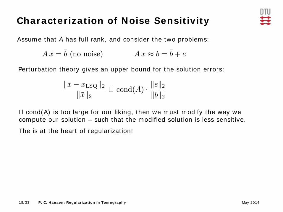
Characterization of Noise Sensitivity

Assume that A has full rank, and consider the two problems:

A ¹x = ¹b (no noise) A x ¼ b = ¹b + e

Perturbation theory gives an upper bound for the solution errors:

k¹x¡ xLSQk2k¹xk2

· cond(A) ¢ kek2k¹bk2

If cond(A) is too large for our liking, then we must modify the way we compute our solution – such that the modified solution is less sensitive.

The is at the heart of regularization!


SVD Analysis – How to Reduce Sensitivity

Recall the two relations:

xLSQ = Ayb = (ATA)¡1AT b; f = R¡1f̂ :

We introduce the singular value decomposition (SVD):

A = U § V T =X

i

ui ¾i vTi ; U; V orthogonal; § = diag(¾1; ¾2; : : :):

Algebraic reconstruction

xLSQ = AT (U §¡2UT ) b

= (V §¡2V T ) AT b

Inverse Radon transform

f = R¤(¡¢)1=2f̂

= (¡¢)1=2R¤f̂

FBP: add a filter here in the frequency domain §¡2 ! ©2 §¡2

© = §2 (§2 + ¸2I)¡1j!j ! ª(!) ¢ j!j

In both methods, we loose the details associated with high frequencies.

cond(A) = ¾1=¾n ! ¾1=¸

Tikhonov: filter the singular values


Matlab Check …

N = 3*24;

theta = 3:3:180;

[A,b,x] = paralleltomo(N,theta,[],N);

[U,S,V] = svd(full(A));

lt = length(theta);

Si = reshape(b,length(b)/lt,lt);

bf = U*pinv(S)'*pinv(S)*U'*b;

SF = reshape(bf,length(b)/lt,lt);

Xbp = reshape(A'*b,N,N);

Xrec = reshape(A'*bf,N,N);


Dealing with a Nonunique Solution

The system A x ≈ b fails to have a unique solution when rank(A) < n, where n is the number of unknowns (the number of columns in A).

• This can happen when the distribution of rays is badly chosen (we saw an example of this in the 2 x 2 example).

• The more common situation is when we less data than unknowns (i.e., too few rays penetrating the object); this happens, e.g.,

• if we need to reduce the X-ray dose,

• or if we have limited time to perform the measurements.

x = x0 + x?; x? 2 N (A)

f = f0 + f?; f? 2 N (Rla)Minimum-norm solution:

xMN = Ayb = AT (A AT )¡1b

xMN 2 R(AT ) ) xMN ? N (A)f = R¤la(¡¢)1=2f̂

f 2 R(R¤la) ) f? = 0

Radon – the limited-angle case:

Infinitely many solutions of the general forms:


Appreciation of Minimum-Norm Solutions The minimum-norm solution deals – in a way – in a very logical way with N(A), the null space of A: don’t try to reconstructruct this component.

The same is true for the filtered solutions: the filter effectively dampens the highly-sensitive components corresponding to small singular values σi.

So: if the subspace R(AT) captures the main features of the object to be reconstructed, then this is a good approach.

Tikhonov Another filtered solution: Cimmino

A smooth test image

Example: underdetermined, limited-angle problem, angles 5,10,15,…,120.


Critique of Minimum-Norm Solutions The minimum-norm solution – while mathematically “nice” – is not guaranteed to provide a good reconstruction; it “misses” information in the N(A) or N(Rla

*).

Examples: underdetermined, limited-angle problems.

Notice that for the limited-angle problem, FBP misses certain geometric structures in the image, associated with the missing projection angles.

These structures are precisely those in the null space of Rla, see, e.g.: • Jürgen Frikel, Sparse regularization in limited angle tomography, Appl. Comput.

Harmon. Anal., 34 (2013), 117–141.

We can find other ways to deal with effectively underdetermined problems!

Tikhonov FBP FBP

True


Approach 1: ART The Algebraic Reconstruction Method (ART) – also known as Kaczmarz’s method – was originally developed to solve full-rank square problems A x = b.

ART has fast initial convergence, and for certain tomo problems is has been the method of choice.

for k = 1; 2; 3; : : :

i = k mod (# rows)

xk+1 = xk + !bi ¡ aTi xk

kaik22ai aTi = ith row of A

end


Regularizing Properties of ART

After some iterations the method slows down – and at this time we are often “close enough” to the desired solution.

During the ¯rst iterations, the iterates xk capture \important" information

in b, associated with the exact data ¹b = A ¹x.

² In this phase, the iterates xk approach the exact solution ¹x.

At later stages, the iterates starts to capture undesired noise components.

² Now the iterates xk diverge from the exact solution and theyapproach the undesiredleast squares solution xLSQ.

”… even if [the iterative method] provides a satisfactory solution after a certain number of iterations, it deteriorates of the iteration goes on.”

This behavior is called semi-convergence, a term coined by Natterer (1986):


Illustration of Semi-Convergence

Ayb

¹x = exact sol.


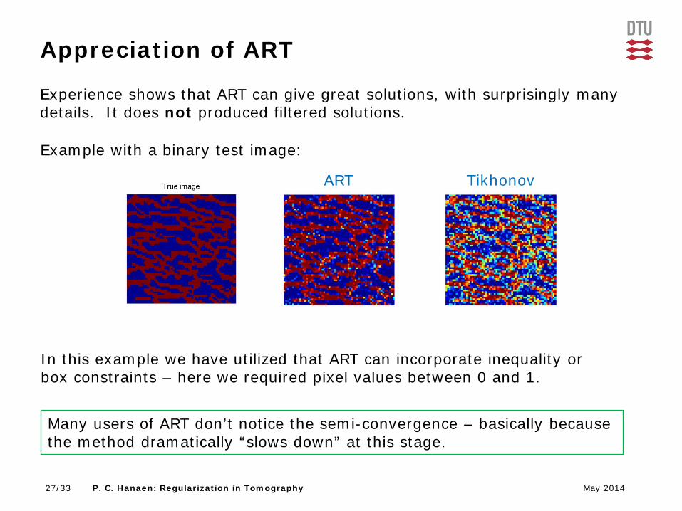
Appreciation of ART

Experience shows that ART can give great solutions, with surprisingly many details. It does not produced filtered solutions.

Example with a binary test image:

Tikhonov ART

In this example we have utilized that ART can incorporate inequality or box constraints – here we required pixel values between 0 and 1.

Many users of ART don’t notice the semi-convergence – basically because the method dramatically “slows down” at this stage.


Appreciation of ART – Contd. Why can ART give so good solutions with high-frequency components?

• It does not correspond to spectral filtering.

• It includes components in the null space, which may be desirable.

• A full theoretical understanding of its superiority is still missing …

Towards some insight.

A certain variant, Symmetric ART, can actually be expressed in a certain ortho- normal basis – and this basis includes the needed high-frequency components!

SVD basis

Basis for sym. ART


Critique of ART

The reconstruction and regularization properties of ART are solely associated with the semi-convergence, and not suited for all types of problems.

Example with a smooth test image:

Tikhonov ART

There is also a need for more general regularization methods … next slide.


Approach 2: Variational Regularization In these methods, the regularization is explicit in the formulation of the problem to be solved:

minxfmis¯t(A; b; x) + ¸¢penalty(L; x)g subject to x 2 C

Di®erent noise:Gaussian: kb¡A xk22Laplace: kb¡A xk1Poisson: kdiag(log(Ax)b¡A xk1Etc.

Norm/energy: kxk22Flatness : kL1 xk22Roughness : kL2 xk22Piecewise smooth : kL1 xk1Etc.

Nonnegativity: x ¸ 0Box constr.: ` · x · uEtc.

Let’s look at this case, known as Total

Variation (TV)

Give smooth solutions


Total Variation Allows Steep Gradients

1-D continuous formulation:

Example (2-norm penalizes steep gradients, TV doesn’t):

TV (g) =°°g0°°

1=

Z

jg0(t)j dt

2-D and 3-D continuous TV formulations:

TV (g) =°° krgk2

°°1

=

Z

krg(t)k2 dt


Underlying assumption or prior knowledge: the image consists (approx.) of regions with constant intensity.

Hence the gradient magnitude (2-norm of gradient in each pixel) is sparse.

TV Produces a Sparse Gradient Magnitude

3 % non-zeros im

age

grad

ient

mag

nitu

de

Experience shows that the TV prior is often so “strong” that it can compensate for a reduced amount – or quality – of data.

TV = 1-norm of the gradient magnitude,

= sum of 2-norm of gradients.


We demonstrated that tomographic reconstruction problems (inverse problems) have stability problems:

• The solution is always sensitive to noise.

• The solution may not be unique.

We looked at different common reconstruction algorithms and explained how the incorporate regularization:

• Filtered back projection – via a low-pass filter

• Tikhonov – via filtering of SVD components

• ART (Kaczmarc) – by stopping the iterations (semi-convergence)

• Variational methods – the regularization is explicit.

We saw that all these algorithms have their advantages and disadvantages, and introduce different artifacts in the solutions.

Conclusions – What to Take Home

regularization in tomographypcha/talks/regtomo.pdf · regularization in tomography dealing with...

Documents