Regulatory Arbitrage andSystemic Liquidity Crises∗

Stephan Luck† Paul Schempp‡

JOB MARKET PAPERLATEST VERSION

November 2015

We derive a novel bank run equilibrium within a standard banking frame-work. Intermediaries optimally rely on wholesale funding to manage liquidityneeds, setting the stage for systemic runs: When some intermediaries are sub-ject to a run, they raise funds by liquidating their assets. Fire sales in turninduce an overall scarcity of liquid funds, depressing asset prices and hencedeteriorating the funding conditions of other intermediaries in the marketfor secured wholesale funding. We apply the concept of systemic runs in amodel in which regulated banks and shadow banks coexist. First, we showthat even without contractual linkages between the two sectors and despitethe absence of runs on regulated banks, shadow banking panics can cause in-solvency of the regulated banking sector. Second, even though some shadowbanking is efficient, from a social planner’s perspective, the shadow bankingsector grows too large in equilibrium due to a pecuniary externality. Third,prudential regulation and central bank interventions change the equilibriumcomposition of the financial system and affect welfare in non-standard ways.

∗We thank Markus Brunnermeier, Martin Hellwig, and Stephen Morris for extensive support and advice.We are also thankful to Tobias Berg, Christoph Bertsch, Felix Bierbrauer, Jean-Edouard Colliard,Brian Cooper, Olivier Darmouni, Peter Englund, Maryam Farboodi, Douglas Gale, Valentin Haddad,Hendrik Hakenes, Sam Hanson, Zongbo Huang, Nobuhiro Kiyotaki, Sam Langfield, Adrien Matray,Anatoli Segura, as well as participants of the summer school in economic theory of the econometricsociety in Tokyo and seminar participants in Princeton and Mannheim, for valuable comments andsuggestions. Financial support by the Alexander von Humboldt Foundation and the Max PlanckSociety is gratefully acknowledged.

†stephan.luck@princeton.edu, University of Bonn, Princeton University, and Max Planck Institute forResearch on Collective Goods, phone: +1 609 454 1462 (US), + 49 (0) 178/7264717 (Germany).

‡schempp@coll.mpg.de, Max Planck Institute for Research on Collective Goods.

1. Introduction

Regulatory arbitrage and the growth of shadow banking have been identified as essential

ingredients to the 2007-09 financial crisis (Financial Crisis Inquiry Commission 2011).

In particular, explicit or implicit contractual linkages between commercial banks and the

shadow banking sector,1 such as liquidity or credit enhancements, have been a source of

fragility (Acharya et al. 2009; Brunnermeier 2009; Hellwig 2009; Acharya et al. 2013).

Accordingly, post-crisis reforms have targeted the contractual channels through which

the turmoil in the shadow banking sector has affected the commercial banking sector

(“Volcker Rule”, “Vickers Commission”, “Liikanen Report”).2 Naturally, the question

arises whether the implemented and proposed reforms are effective. Can the prohibition

of contractual linkages between commercial banks and non-bank financial institutions

be successful in eliminating fragilities arising from regulatory arbitrage?

We formalize a novel argument as to why the prohibition of explicit and implicit

contractual linkages may be insufficient. We argue that a financial panic originating

in the shadow banking sector can be contagious and can affect the regulated banking

sector via pecuniary channels: Suppose that a large-scale withdrawal from the shadow

banking sector is imminent. In this case, shadow banks will be forced to raise funds

by liquidating assets in a fire sale, potentially triggering an overall scarcity of liquid

funds in the money market. Hence, the conditions under which regulated banks obtain

wholesale funding also deteriorate, even though the fundamentals remain unchanged.

Runs on shadow banks may thus cause illiquidity and insolvency of regulated banks,

even without runs inside the banking sector and in the absence of contractual linkages

between commercial banks and non-bank financial institutions.

The formalization of this pecuniary contagion channel requires us to develop a new

type of run equilibrium. The theoretical foundation is the interplay between two fric-

tions. There is the standard friction in bank run models that contracts cannot be made

contingent on agents’ types (see, e.g., Diamond and Dybvig 1983; Goldstein and Pauzner

2005).3 We add a second friction that prevents intermediaries from contracting with fu-

1We use the term “shadow banking” to describe banking activities (risk, maturity, and liquidity trans-

formation) that take place outside the regulatory perimeter of banking and do not have direct access

to public backstops, but may require backstops to operate; compare Pozsar et al. (2013), FSB (2013),

Claessens and Ratnovski (2014), and Luck and Schempp (2014a).2See Section 619 of the Dodd-Frank Act (“Volcker Rule”), the Financial Services Act (“Report of the

Vickers Commission”), and the proposed EU law on bank structural reform (“Liikanen Report”);

see Section 2 for a more detailed description of shadow banking activities prior to and during the

financial crisis of 2007-09 as well as on the regulatory response after the crisis.3Following Bryant (1980) and Diamond and Dybvig (1983), there is an extensive literature on bank

1

ture providers of liquidity (e.g., as in Holmstrom and Tirole 1998, 2011).4

The interaction of these two frictions gives rise to a novel class of bank run equilibria in

which runs on some intermediaries affect the funding conditions of other intermediaries.

We refer to these types of runs as systemic runs. The underlying mechanism is that runs

on some intermediaries may lead to a binding cash-in-the-market constraint (see, e.g.,

Allen and Gale 1994, 2007). Even though the market for wholesale funding is perfectly

competitive, once a run induces a scarcity of liquid funds, liquidity providers will be

able to earn rents. Hence, those intermediaries that are not subject to a run, but rely

on raising liquid funds via the market, are affected via a deterioration of their funding

liquidity.

In contrast to previous work, the systemic aspect of runs does not result from interbank

linkages (Allen and Gale 2000; Freixas et al. 2000; Farboodi 2015) or correlated risks

(Acharya and Yorulmazer 2007, 2008). The contagion operates via the exposure to a

common pool of liquidity and deteriorating funding conditions. We argue that the notion

of systemic runs is stronger than in previous work in which contagion operates via fire

sales (Uhlig 2010; Diamond and Rajan 2005, 2011; Martin et al. 2014b).

The particular feature of our model is that even in the absence of any fundamental risk

or contractual linkages between intermediaries, runs on some intermediaries necessarily

affect other intermediaries, and may even make a run on all intermediaries inevitable.

The systemic property stems from the fact that liquidity management relies on short-

term wholesale funding, exposing intermediaries to movements in asset prices that result

from runs elsewhere. Unlike in other work (Shleifer and Vishny 1997, Brunnermeier 2009,

and Greenwood et al. 2015, Adrian and Shin 2014), there is no difference between market

and funding liquidity of intermediaries in our model. The conditions under which assets

can be sold and under which funds can be borrowed are isomorphic. An intermediary

that is subject to a run is facing tight market liquidity, and an intermediary that is not

subject to a run is facing tight funding liquidity, where the former causes the latter.

We apply the concept of systemic runs to a model in which regulated banks and shadow

runs on single institutions. See, e.g., the literature regarding information-based runs (Jacklin and

Bhattacharya 1988; Postlewaite and Vives 1987; Chari and Jagannathan 1988), models with macroe-

conomic risk (Hellwig 1994; Allen and Gale 1998), contagion via interbank linkages (Bhattacharya

and Gale 1987; Allen and Gale 2000), models that combine macroeconomic risk and strategic uncer-

tainty (Rochet and Vives 2004; Morris and Shin 2003; Morris and Shin 2010), and dynamic runs (He

and Xiong, 2012).4The friction that agents cannot commit to future financing is used in banking contexts by Uhlig (2010),

Bolton et al. (2011), Luck and Schempp (2014b), and Hakenes and Schnabel (2015), among others.

Moreover, the friction also arises naturally in banking models in OLG environments, as in Qi (1994)

and Martin et al. (2014a,b).

2

banks coexist. Three important implications follow: First, the prohibition of contrac-

tual linkages between commercial banks and non-bank banking entities is insufficient to

safeguard the regulated banking sector. Even though there are no contractual linkages

between the sectors, no fundamental risk of insolvency, and no prospect of panics at

regulated and insured banks, insured institutions may yet turn illiquid and insolvent.

Funding conditions may deteriorate due to a run on uninsured shadow banks. The possi-

bility of regulatory arbitrage thus challenges the conventional wisdom that the provision

of a safety net can eliminate strategic complementarity between depositors at zero cost.

If the extent of regulatory arbitrage cannot be controlled, a deposit insurance eliminates

runs only partially and the deposit insurance scheme is costly as it needs to live up to

its promise in case of systemic liquidity crises.

Second, while the existence of shadow banks may be efficient in our model, the shadow

banking sector is too large in equilibrium. Hence, we do not argue that regulatory

arbitrage is diabolic per se. A certain degree of regulatory arbitrage is efficient and

desirable, as shadow banks make efficient use of the disciplining effect of short-term

debt.5 However, we find that regulatory arbitrage is excessive from a social planner’s

perspective. The underlying mechanism is a pecuniary externality that operates through

fire-sale prices. When consumers decide whether to deposit at a shadow bank or at a

regular bank, agents face the following trade-off: A regular bank offers a low interest

payment as it is subject to regulatory cost, but the safety net eliminates all risk. In

contrast, a shadow bank offers a higher interest, but it comes with the prospect of panic-

based runs. When making their choice, depositors do not internalize that depositing in

the shadow banking sector reduces the equilibrium fire-sale price.6 Lower fire-sale prices

in turn have three negative effects: First, they increase the probability of runs taking

place.7 Second, they reduce the amount of funds available to shadow banks in case of a

5On the disciplining effect of short-term debt, see Calomiris and Kahn (1991) and Diamond and Rajan

(2001). Our argument complements other arguments why shadow banking may be desirable, such

as comparative advantages in securitizing assets (compare, e.g., Gennaioli et al. 2013; Hanson et

al. 2015), or by relaxing imperfect prudential constraints and utilizing self-regulating reputational

concerns (see Ordonez 2013; Huang 2014).6The fact that a pecuniary externality impacts welfare is reminiscent of findings in the literature on

pecuniary externalities in an incomplete markets setup; compare, e.g., Lorenzoni (2008). See also

Bengui and Bianchi (2014) for a sectoral model with circumvention of regulatory requirements and

Diamond and Rajan (2011) for a banking model with fire sales. In our model, the intuition for why

the pecuniary channel affects welfare is similar; however, the exact mechanisms cannot be compared,

as we only do a partial equilibrium analysis.7In our model, runs occur with a positive probability as in Cooper and Ross (1998), but we assume

that the probability is a function of the model’s variables and decreasing in the fire-sale price as in

Gertler and Kiyotaki (2015).

3

run. Third, they increase the shortfall of funds in the regulated banking sector and thus

the funding required for the deposit insurance scheme.

Finally, if the extent of regulatory arbitrage cannot be controlled, the welfare effects of

prudential regulation and central bank interventions are ambiguous. Restricting whole-

sale funding for regulated banks, as in the liquidity regulation of Basel III, would allow

the regulated banking sector to be shielded from adverse consequences originating out-

side the sector. However, it would also lead to allocative inefficiencies in the banking

sector and would thus induce more regulatory arbitrage, i.e., a larger shadow banking

sector, making severe fire sales even more severe. Liquidity regulation may thus backfire:

even though it stabilizes the regulated banking sector, overall financial stability may be

weakened.

Likewise, central bank interventions such as lender of last resort (LoLR) and market

maker of last resort (MMLR) shield commercial banks from adverse events originating

in the shadow banking sector. Both types of interventions increase the relative attrac-

tiveness of shadow banking by reducing the need of regulated banks to sell assets in a

fire sale, making the fire sale less severe for shadow banks. Interestingly, the anticipa-

tion of central bank interventions creates systemic risk not via the standard channels of

moral hazard with respect to risk choices (Acharya and Yorulmazer 2008) or the degree

of maturity mismatch (Farhi and Tirole 2012), but solely via changing the composition

of the financial system.

The relevance of the risk of systemic runs in our current financial system becomes

clear if we have a look at the pure quantities involved. After the crisis of 2007-09,

shadow banking remains a concern for regulators, economists, and market participants.

According to the FSB (2014), shadow banking activities globally amount to 25% of total

financial assets, 50% of assets held by the banking system, and 120% of GDP on average.

Moreover, shadow banking activities as measured by overall assets have grown relative

to assets financed by the regular banking sector since 2008. When narrowing down to

those shadow banking institutions that have no legal connection to commercial banks,

they still hold about 30% of all financial assets in both, the US as well as in the euro

area. Also, these types of measures have continued to grow since 2008, and their growth

has outpaced that of the banking sector. At the same time, despite having declined since

2007, wholesale funding still makes up around 15-25% of the regulated banks’ liabilities8

8The numbers vary depending on what types of funding are counted as wholesale funding and whether

long-term funding is excluded or not. Typical definitions include short-term unsecured funds, inter-

bank loans, commercial paper (CP), and wholesale certificates of deposit (CDs), repurchase agree-

ments (repos), swaps, and asset-backed commercial paper. Long-term funding includes bonds is-

suance and various forms of securitization, including covered bonds and private-label mortgage-backed

4

in the United States and in the euro area (International Monetary Fund 2013; European

Central Bank 2014). Thus, the two main ingredients of our model are present in our

current financial system: A large shadow banking sector and regulated banks’ exposure

to the risk of changing conditions in the market for wholesale funding.

We proceed as follows: Section 2 gives a brief overview of shadow banking prior to

and during the crisis of 2007-09 and the regulatory response after the crisis. Sections 3

and 4 describe the setting and the concept of systemic runs. Section 5 shows how deposit

insurance combined with a capital requirement can eliminate the fragility, but also how

regulatory arbitrage reintroduces fragility even in the absence of contractual linkages.

Section 6 derives the equilibrium size of the shadow banking sector and shows that

regulatory arbitrage is excessive in equilibrium. Finally, Section 7 discusses the effects

of wholesale funding restrictions, central bank interventions, and liquidity guarantees.

Section 8 concludes.

2. Shadow Banking, the Crisis of 2007-09, and the Regulatory

Response

Prior to the 2007-09 financial crisis, many commercial banks had set up off-balance-sheet

conduits to finance long-term real investment by issuing short-term debt (Pozsar et al.,

2013). From an ex-post perspective, it appears that off-balance-sheet banking had to a

large extent been conducted to circumvent existing capital regulation (see, e.g., Acharya

et al., 2013).9 A typical intermediation chain would look as follows: special purpose

vehicles such as asset-backed commercial paper conduits were set up to finance mortgage-

backed securities (MBS) and other asset-backed securities (ABS) by issuing asset-backed

commercial papers (ABCP) and medium-term notes (MTN), which in turn where mostly

held by money market mutual funds (MMF). Conduits were either granted explicit credit

or liquidity guarantees (credit or liquidity enhancements), or implicit guarantees as in

the case of structured investment vehicles (SIV). I.e., less than 30% of the conduits

had received outright guarantees. However, most other conduits that were set up by

commercial banks had relational contracts with their parent companies. Reputational

concerns ensured that parent companies would not let their shadow banking subsidiaries

default; see particularly Segura (2014).

In the summer of 2007, increased delinquency rates on subprime mortgages ultimately

led to the collapse of the conduits’ main source of funding:10 the market for ABCP (see,

securities.9To some observers, this had already been clear prior to the crisis; see Jones (2000).

10The trigger is widely acknowledged to be BNP Paribas suspending convertibility of three of its funds

5

e.g., Kacperczyk and Schnabl, 2009; Covitz et al., 2013). The collapse forced banks

to take the conduits’ assets and liabilities on their balance-sheets, and their insufficient

equity cushions created severe solvency issues (Acharya et al., 2013).11

The post-crisis narrative has been that shadow banking could only become so large be-

cause most shadow banks were set up and operated by commercial banks, which in turn

had access to the safety net (i.e., the discount lending window, deposit insurance, im-

plicit bailout guarantees, see Financial Crisis Inquiry Commission, 2011). Consequently,

regulatory reforms have tried to close loopholes in regulation by outright prohibition of

contractual links between depository institutions and other parts of the financial system.

The reform proposals include a ring-fencing of depository institutions and systemic ac-

tivities (Report of the Vickers Commission, enacted as Financial Services Act in 2013),

separation between different risky activities (“Report of the European Commission’s

High-level Expert Group on Bank Structural Reform”, known as the Liikanen Report),

and prohibition of proprietary trading by commercial banks (Section 619 of the Dodd-

Frank Act, referred to as the “Volcker Rule”).

Section 619 of the Dodd-Frank Act – besides prohibiting banking corporations from

conducting proprietary trading – also prevents banking corporations from entering into

transactions with funds for which they serve as investment advisers. Therefore, conduit

operations by commercial banks, in particular rescuing conduits, are heavily restricted.

Likewise, following the Report of the Vickers Commission, the Financial Services Act

in 2013 limits the exposure of depository institutions to other financial entities within

the same bank holding company (BHC). This also implies that any type of outright

guarantees or any support in distress from depository institutions to shadow banking

subsidiaries becomes impossible. In a similar spirit, the Liikanen Report promotes a

mandatory separation of proprietary trading and other high-risk trading (“trading en-

tity”) from commercial banking (“deposit bank”), trying to restrict contractual con-

nections between standard banking and market-based activities. Hence, the regulatory

paradigm throughout all three jurisdictions has been that ex-ante or ex-post support to

off-balance-sheet activities shall be prohibited or restricted. In the following, we ana-

lyze whether this is sufficient to enhance financial stability in the presence of regulatory

that were exposed to risk of subprime mortgages bundled in ABS.11Subsequent to the runs on ABCP, there had been counterparty runs at Bear Stearns’ and Lehman’s

tri-party repo programs (Copeland et al., 2014). Moreover, there had been severe contractions in

overall repo funding throughout 2007 and 2008 (Gorton and Metrick, 2012), which was, however, less

important than the contraction in the market for ABCP (Krishnamurthy et al., 2014). Finally, the

Lehman failure triggered a large-scale withdrawal from the prime money market industry (Schmidt

et al., 2014).

6

arbitrage.

3. Setup

Consider an economy that goes through a sequence of three dates, t ∈ {0, 1, 2}. There is

a single good that can be used for consumption as well as for investment. The economy

is populated by three types of agents: consumers, intermediaries, and investors.

Technologies

Altogether, there are three technologies available for investment (see a summary of the

payoff structure in Table 1). Storage is available in t = 0, 1, transforming one unit

invested in t into one unit in t + 1. In addition, two illiquid technologies are available

for investment in t = 0: a “productive technology” and an unproductive “shirking

technology”. Both technologies are technologically illiquid, i.e., the physical liquidation

rate in t = 1 is assumed to be zero. However, claims on the technologies’ future returns

may nonetheless be traded in a secondary market in t = 1.

The return properties of the illiquid technologies in t = 2 are as follows: One unit

invested in the productive technology yields a safe return of R > 1 units in t = 2. One

unit invested in the shirking technology yields a safe return of Rshirk in t = 2. Moreover,

this technology yields a private benefit B > 0 in t = 2 which is non-pledgeable. We

assume that Rshirk +B ≤ 1. I.e., the shirking technology is inefficient, but may give rise

to moral hazard.

t = 0 t = 1 t = 2

Storage in t = 0 -1 1 0

Storage in t = 1 0 -1 1

Productive technology -1 0 R

Shirking technology -1 0 Rshirk +B

Table 1: Payoff structure of technologies

Consumers

There is a continuum of consumers with mass one. Each consumer is endowed with 1

unit of the good in t = 0. There are two types of consumers, patient and impatient

consumers: a fraction π is impatient and derives utility only from consumption in t = 1,

u(c1), and a fraction 1−π is patient and derives utility only from consumption in t = 2,

u(c2). We restrict attention to CRRA utility, i.e., the baseline utility function has the

form u(ct) = 11−η c

1−ηt , with η > 1.

7

The demand for liquid assets arises as consumers face idiosyncratic uncertainty with

respect to their preferred date of consumption. Initially, the probability of being impa-

tient is identical and independent. At date 1, each consumer privately learns his type,

which can be considered as a liquidity shock. The fact that types are private informa-

tion implies that contracts cannot be made contingent on types. This is the standard

friction that gives rise to the possibility of bank runs when illiquid assets are financed

by short-term debt.12

A consumption profile (c1, c2) denotes an allocation where an impatient consumer

receives c1 and a patient consumer receives c2. As of date 0, such a consumption profile

induces an expected utility of

U(c1, c2) = πu(c1) + (1− π)u(c2) =1

1− η

[πc1−η1 + (1− π)c1−η2

]. (1)

We restrict the action space of consumers to investing in storage and to interacting

with intermediaries. In particular, we assume that consumers cannot invest directly in

the productive technology.13

Intermediaries

There is a mass m of intermediaries.14 While consumers cannot invest in the productive

technologies directly, intermediaries face no investment restrictions. Intermediaries have

no market power and compete for the consumers’ funds in order to invest on their behalf.

Moreover, intermediaries have an endowment which they can invest in the intermediation

business or in some outside option. We assume that the endowment is sufficiently large

such that no result will be driven by the aggregate intermediaries’ endowment becoming

a binding resource constraint.

Intermediaries care about their wealth at date 2 and have an outside option. The

outside option is assumed to induce a required return of ρ > R in t = 2 for each unit

invested in t = 0. As the required return is larger than the productive technologies’

returns, it is costly for the consumers if the intermediaries use their endowment for

investment. This assumption makes it costly to use a skin-in-the-game mechanism in

order to provide intermediaries with incentives to prevent shirking. Later on, ρ will

12Compare to the classic bank run literature, e.g., Diamond and Dybvig (1983), Bhattacharya and Gale

(1987), and Allen and Gale (1998, 2000, 2007).13This allows us to abstract from issues that arise via the coexistence of financial markets and inter-

mediaries. In Section B of the appendix, we argue briefly why we can focus on a banking solution

directly, i.e., why a banking solution dominates a financial markets solution.14It is assumed that m is small compared to the mass of depositors such that each bank has a very

large number of depositors, and thus does not face aggregate liquidity risk by a law of large numbers

argument.

8

therefore also be referred to as regulatory costs.

The assumption is a shortcut for assuming that some market imperfections make issu-

ing equity more costly than debt. The standard argument why equity is costly is based

on adverse selection concerns (Myers and Majluf, 1984). Other, more recent reasonings

are for instance a detrimentally high cost of renegotiating with existing creditors and an

associated leverage-ratchet effect (Admati et al., 2013), non-pecuniary benefits to bank

owners (Adrian and Shin, 2011).

Investors

There is a continuum of investors of mass n. Investors are modeled as liquidity providers

to intermediaries, i.e., as agents or institutions that supply liquid funds on the money

market.15 Investors are born at date 1 and care about their wealth at date 2. They are

assumed to have a technology with a return of µ as an outside option, where µ ∈ [1, R].

That is, investors have a required return of µ in t = 2 for each unit they transfer to

intermediaries in t = 1.

Investors are endowed with A/n units of the good, and the investors’ aggregate en-

dowment is given by A. The endowment A will be one of the crucial parameters of the

model: while it may be sufficiently high to allow investors to supply liquidity in normal

times, it may lead to a binding cash-in-the-market constraint in case of systemic runs.

Moreover, the fact that investors are born not before t = 1 is the second important

friction in our model. It implies that from the t = 0 perspective, intermediaries cannot

write contracts with investors and thus their funding conditions may deteriorate.16

4. Intermediation, Bank Runs, and Systemic Runs

In the following, we derive the first-best allocation and show how it can be implemented

by intermediaries. We then show that not only single intermediaries can be subject to

runs, but also that runs can be systemic, i.e., runs on some intermediaries necessarily

impact those intermediaries that are not subject to runs.

15Investors should be seen as the standard providers of liquidity on the money market, i.e., agents and

institutions with information on and access to the money market: banks with current high liquidity

inflow, hedge funds, pension funds, or larger corporations with abundant liquid funds. Later we will

also consider the central bank as an actor that competes with investors.16See, e.g., Holmstrom and Tirole (1998, 2011) on assuming limited commitment of future financing. In

the context of banking models, the assumption is made, e.g., by Bolton et al. (2011), Martin et al.

(2014a,b), Luck and Schempp (2014a), and Hakenes and Schnabel (2015).

9

4.1. First best

We derive the allocation that maximizes the expected utility of consumers, subject to

the participation constraints of intermediaries and investors, and subject to the resource

constraints. We refer to the resulting allocation as the first-best allocation and denote

it by (c∗1, c∗2).

Let I denote the amount that intermediaries invest in the productive technology, and

Ishirk the investment in the shirking technology. In the first best, the shirking technology

is not used as the productive technology strictly dominates the shirking technology,

i.e., Ishirk = 0. Moreover, let e0 denote the amount that intermediaries invest in the

intermediation business at date 0, and e2 what they receive at date 2. Given the required

return of intermediaries ρ > R, optimality implies that e0 = e2 = 0. Denote by L1 the

amount of goods that get transferred from investors to consumers in t = 1 (“liquidity”),

and L2 the amount of goods transferred back to investors in t = 2.

The optimization problem for the first best is the following:

max(c1,c2,I,L1,L2)∈R5

+

πu(c1) + (1− π)u(c2), (2)

subject to πc1 ≤ (1− I) + L1, (3)

(1− π)c2 ≤ IR− L2, (4)

L2 ≥ µL1, (5)

L1 ≤ A, and (6)

I ≤ 1. (7)

The budget constraints for date one and two are given by (3) and (4). Investors may

transfer L1 to consumers in t = 1 in exchange for L2 units in t = 2. (5) represents the

participation constraint of investors. The resource constraint on the investors’ provision

of “liquidity” is given by (6), and (7) denotes the constraint on the initial investment.

Depending on the model parameters A,R, µ, and π, as well as on the shape of the

utility function, the first-best program has three solution candidates. As discussed in

detail in Section A of the appendix, investment in storage is only optimal if A is small,

and becomes unnecessary when A is sufficiently large. For the remaining part of the

paper we restrict attention to the parameter space in which intermediation optimally

relies exclusively on investors providing liquid funds at date 1. That is, it is optimal to

invest exclusively in the productive technology, i.e., I∗ = 1 and the storage technology

is redundant. This restriction is formalized by the following:

10

Assumption 1. A ≥ ξ ≡ πµ−1η R

(1−π)+πµ1−1η

.

This allows us to characterize the first-best allocation:

Lemma 1 (First-best Allocation). The first-best allocation is characterized by

I∗ = 1, L∗1 = πc∗1, L∗2 = µπc∗1, and Ishirk = e0 = e2 = 0,

and the optimal consumption profile is given by

c∗1 = µ− 1η

R

(1− π) + πµ1− 1

η

and c∗2 =R

(1− π) + πµ1− 1

η

. (8)

Under Assumption 1, it is optimal to invest exclusively in the illiquid productive

technology and entirely rely on investors to provide funds for those that are subject to

a liquidity shock at date 1. When using investor funds to satisfy the demand for liquid

assets in t = 1, the technological rate of substitution between date 1 and 2 is given

by the investors’ required return µ. Therefore, the risk-sharing between early and late

consumers is described by the FOC u′(c1) = µu′(c2), and it holds that R > c∗2 > c∗1 >

R/µ, where R/µ is the rate of return on the productive asset between date 0 and 1,

when it is traded against liquid funds from investors.17

4.2. Implementation

In the following, we show that the first-best allocation can be implemented by interme-

diaries issuing demand-deposit contracts to finance the illiquid investment.

Lemma 2 (Intermediation). There exists a subgame-perfect Nash equilibrium in which

the first-best consumption profile (c∗1, c∗2) is implemented by the intermediaries offering

demand-deposit contracts. Intermediaries rely on secured wholesale funding by investors

in order to manage liquidity needs.

The implementation of the first-best allocation via demand-deposit contracts offered

by intermediaries has three dimensions. The first dimension is that demand-deposit

contracts allow consumers to share their risk optimally, and at the same time incentives

17In the banking model of Diamond and Dybvig (1983) – which is nested in our model for the class

of constant relative risk aversion – risk-sharing between patient to impatient consumers is optimal,

implying that R > cDD2 > cDD1 > 1, where 1 is the technological rate of return between date 0 and 1

(storage).

11

are such that agents reveal their type in t = 1 truthfully (e.g., as in Diamond and Dybvig,

1983). The latter is incentive-compatible as c∗2 > c∗1.

The second dimension is the disciplining effect of short-term debt. We discuss why

demand deposits are disciplining in our setup in detail in the Section C of the appendix.18

The underlying logic is as in Calomiris and Kahn (1991) and Diamond and Rajan (2001):

Demand deposits allow the prevention of shirking. Intermediaries, when investing on

behalf of the financiers, are subject to moral hazard as they may have incentives to invest

in the shirking technology to capture the private benefit B. Whenever an intermediary

has invested in the shirking technology, consumers learn about it at t = 1 and have an

incentive to withdraw collectively. As the debt is demandable, this is in fact possible.

Moreover, as the private benefit accrues not before t = 2, the intermediary will thus not

be rewarded for shirking, and have no incentive to do so in the first place.

The third dimension is raising funds from investors to pay out consumes at the interim

date. Intermediaries invest exclusively in the illiquid assets and need to raise funds from

investors in order to serve withdrawing consumers at date 1. We consider two types

of isomorphic institutional arrangements on how intermediaries can obtain funds from

investors in order to manage the consumers’ liquidity demand: asset sales and secured

wholesale funding.

In order to raise funds via asset sales, an intermediary must sell an overall amount of

πc∗1/(R/µ) units of claims on his investments at price p = R/µ per unit (which we define

as the “fundamental value” of the asset) to the investors. An investor receives an asset

that promises a cash-flow of R in t = 2 for R/µ, and thus earns a return µ, satisfying

her participation constraint.

An alternative arrangement is “secured wholesale funding”. As the fundamental value

of the asset is R/µ, the first best could be implemented by the following collateralized19

debt contract: At date 1, the intermediary receives an amount of liquidity L1 = πc∗1,

which can be used to pay out those consumers who withdraw out of a consumption

motive. In exchange, the intermediary promises to pay back L2 = µπc∗1, implying a

gross interest rate of r = µ. Moreover, the intermediary pledges an amount of assets

πc∗1/(R/µ) as collateral. This collateral has a “fundamental value” of πc∗1 at date 1, and

a value of µπc∗1 at date 2. Thus, collateralizing claims gives investors full seniority. They

are thus able to earn their required return with certainty, ensuring participation.

18As discussed in the appendix, there are also equilibria with partial shirking, which can, however, be

ruled out by restricting investment decisions to be binary.19Importantly, claims have to be secured and collateralized, thus giving the investors de facto senior-

ity. Otherwise, strategic complementarity among investors may arise; compare Luck and Schempp

(2014b).

12

Importantly, the two institutional arrangements – asset sales and collateralized bor-

rowing – are isomorphic in our setup and it holds that the interest rate can be expressed

as r = R/p. For expositional purposes, we assume that intermediaries conduct secured

wholesale funding in normal times and asset sales (fire sales) when they are subject to

a run.

4.3. Bank runs and systemic runs

While short-term debt can have a disciplining effect in our model, it is also a source of

fragility: the model exhibits multiple equilibria in the t = 1 subgame. Runs on single

intermediaries always constitute an equilibrium for the same logic as in standard bank

run models with maturity transformation. If all consumers of a particular intermediary

withdraw, this intermediary becomes insolvent, as she can raise at most R/µ units of

liquidity at date 1 by selling all her assets. However, the consumers are altogether entitled

to c∗1 > R/µ at date 1. If a patient consumer has a belief that all other consumers

withdraw, she can either withdraw and to get R/µ in t = 1,20 or she can wait until

t = 2 and receive nothing. Thus, withdrawal is the best response to withdrawal of all

other agents. The bank-run risk results from the demandable nature of deposit contracts

which is necessary because the information friction concerning the consumer types makes

contingent contracts unfeasible. Intermediaries cannot distinguish whether an individual

is withdrawing out of a consumption or out of a panic motive.

Our analysis, however, goes beyond the classical bank-run problem and asks: When

do runs on some intermediaries impact other intermediaries? Runs can become systemic

via the interaction of the standard friction of non-observable types with the second fric-

tion that prevents intermediaries from contracting with investors at the initial date. If

intermediaries could settle with investors on funding conditions initially, they would be

unaffected when other intermediaries are subject to a run. However, because such con-

tracts are not feasible, intermediaries may face tightening funding conditions once other

intermediaries have to sell assets. Here, the amount of investors’ funds A plays a crucial

role because, depending on A, our model features qualitatively different run equilibria.

If the amount of funds A is sufficiently large, runs on some intermediaries cannot affect

market conditions, and thus they cannot affect other intermediaries. However, if A is

limited, the situation is different: If sufficiently many intermediaries are subject to a run,

then liquidity becomes scarce relative to the demand for liquid funds.21 In this case, the

20We abstract from a sequential-service constraint throughout the paper. We assume that in case of

illiquidity, all funds available are distributed evenly across all consumers who wish to withdraw.21We follow the standard bank run literature in assuming that deposits when withdrawn are consumed

13

market for liquidity clears at terms that are unfavorable for all intermediaries that have

to raise funds from investors.

Since we are interested in the latter case, we assume that the secondary market has

limited depth, i.e., that A is not arbitrarily high. This implies that liquidity is not

globally abundant, and cash-in-the-market pricing prevails if sufficiently many assets

are sold. Technically, this requires the following:

Assumption 2. A < R/µ.

Suppose a mass α of intermediaries are subject to a run, whereas the remaining 1−αare not. The following result holds:

Proposition 1 (Systemic Runs). Consider an equilibrium of the t = 1 subgame in which

α intermediaries are subject to a run. This run is a “systemic run”, i.e., it deteriorates

the funding conditions of all intermediaries, if α > α, where

α =A− πc∗1R/µ− πc∗1

< 1.

If α > α, the run on α intermediaries affects all intermediaries. In particular, also

those 1 − α intermediaries that are not subject to a run face deteriorated funding con-

ditions.22

The underlying mechanism is as follows: The α intermediaries that are subject to

a run must sell all their assets in order to raise as many liquid funds as possible. In

addition, the 1−α intermediaries need to raise a total amount of liquidity of (1−α)πc∗1 in

order to serve impatient consumers. At price p = R/µ, all intermediaries taken together

would sell α+(1−α)πc∗1/(R/µ) units of the asset, thus raising an amount of liquidity of

αR/µ+ (1− α)πc∗1. If this liquidity demand is smaller than the amount of liquid funds

and not redeposited. Without this restriction, further frictions would be needed to explain systemic

runs, such as frictions in interbank trade, as pointed out, e.g., by Skeie (2008).22Notice that not every α ∈ [0, 1] can necessarily prevail in equilibrium as for α sufficiently large, a

deterioration of funding conditions may necessarily lead to a run on all intermediaries. Let us define

α =A− πc∗1

πc∗1RR−(1−π)c1∗

− πc∗1.

If it holds that α < 1, then there exists no equilibrium with α ∈ (α, 1), for the following reason: If

there is a run on α intermediaries, the funding conditions for the remaining intermediaries are such

that they can only pay out exactly c2 = c∗1 to their patient consumers at date 2. Thus, whenever

α > α, it is the dominant strategy of all consumers at all intermediaries to withdraw early, so α = 1

is the only remaining equilibrium.

14

A, the market does actually clear at p = R/µ. This is the case if α ≤ α. Otherwise, i.e.,

if α > α, the market clears at a cash-in-the-market price a la Allen and Gale (1994). The

cash-in-the-market price is equal to the ratio of the funds available, A, to the amount of

assets that need to be sold at price p, which is given by α+ (1− α)πc∗1/p.

The fire-sale price as a function of α is given by

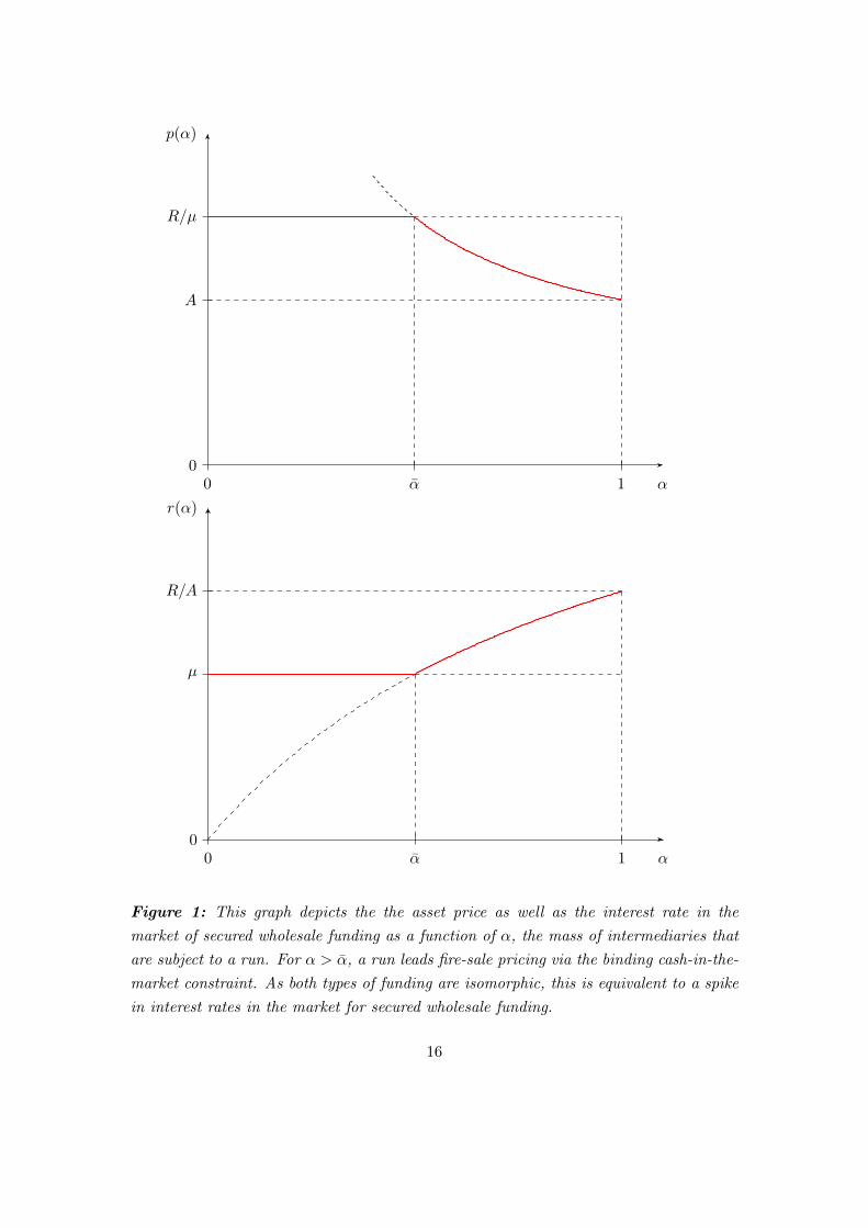
p(α) =

R/µ if α ≤ αA−(1−α)πc∗1

α if α > α.(9)

An economy-wide run is necessarily systemic because it induces cash-in-the-market

pricing, p(1) = A < R/µ. Thus, in a (potentially off-equilibrium) scenario where all

intermediaries but one experience a run, the particular intermediary who is not subject

to a run would still face deteriorated funding conditions.

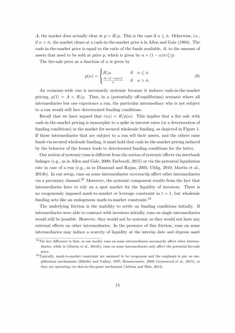
Recall that we have argued that r(α) = R/p(α). This implies that a fire sale with

cash-in-the-market pricing is isomorphic to a spike in interest rates (or a deterioration of

funding conditions) in the market for secured wholesale funding, as depicted in Figure 1.

If those intermediaries that are subject to a run sell their assets, and the others raise

funds via secured wholesale funding, it must hold that cash-in-the-market pricing induced

by the behavior of the former leads to deteriorated funding conditions for the latter.

Our notion of systemic runs is different from the notion of systemic effects via interbank

linkages (e.g., as in Allen and Gale, 2000; Farboodi, 2015) or via the potential liquidation

rate in case of a run (e.g., as in Diamond and Rajan, 2005; Uhlig, 2010; Martin et al.,

2014b). In our setup, runs on some intermediaries necessarily affect other intermediaries

via a pecuniary channel.23 Moreover, the systemic component results from the fact that

intermediaries have to rely on a spot market for the liquidity of investors. There is

no exogenously imposed mark-to-market or leverage constraint in t = 1, but wholesale

funding acts like an endogenous mark-to-market constraint.24

The underlying friction is the inability to settle on funding conditions initially. If

intermediaries were able to contract with investors initially, runs on single intermediaries

would still be possible. However, they would not be systemic as they would not have any

external effects on other intermediaries. In the presence of this friction, runs on some

intermediaries may induce a scarcity of liquidity at the interim date and depress asset

23The key difference is that, in our model, runs on some intermediaries necessarily affect other interme-

diaries, while in (Martin et al., 2014b), runs on some intermediaries only affect the potential fire-sale

price.24Typically, mark-to-market constraint are assumed to be exogenous and the emphasis is put on am-

plification mechanisms (Shleifer and Vishny, 1997; Brunnermeier, 2009; Greenwood et al., 2015), or

they are operating via skin-in-the-game mechanism (Adrian and Shin, 2014).

15

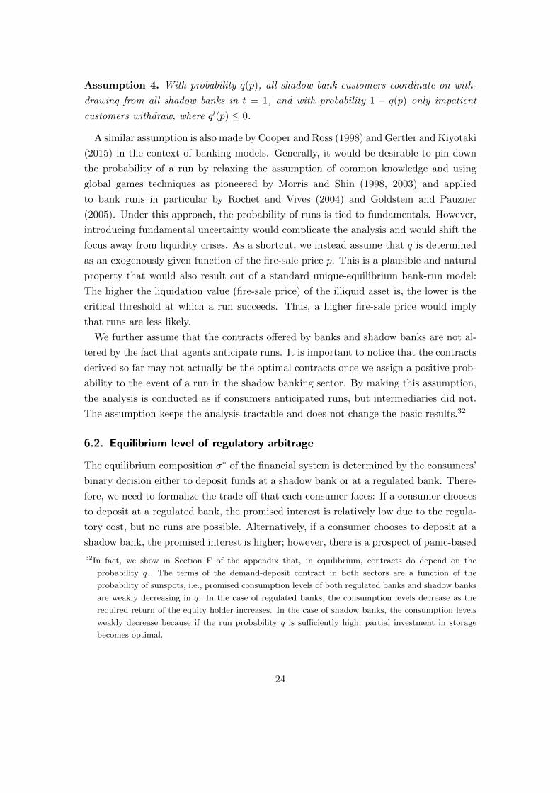
00

R/µ

A

p(α)

αα 1

00

R/A

µ

r(α)

αα 1

Figure 1: This graph depicts the the asset price as well as the interest rate in the

market of secured wholesale funding as a function of α, the mass of intermediaries that

are subject to a run. For α > α, a run leads fire-sale pricing via the binding cash-in-the-

market constraint. As both types of funding are isomorphic, this is equivalent to a spike

in interest rates in the market for secured wholesale funding.

16

prices. In this case, even though investors are competitive, they earn a rent, as liquidity

is scarce relative to demand. Thus, they can purchase assets at discounts or, equivalently,

charge higher interest rates and demand more collateral. Given that intermediaries that

are not subject to a run nonetheless need to raise liquid funds in order to serve those

consumers that withdraw out of a consumption motive, they are necessarily affected

by deteriorating market conditions. The need for short-term financing thus acts like an

endogenous mark-to-market constraint, creating an externality of runs via a deterioration

of funding conditions. This finding is key to understanding the sectoral effects in the

extended model featuring regulated banks and shadow banks in the next section.

5. Banks and Shadow Banks

In this section, we first show that a deposit insurance scheme25 accompanied by a capital

requirement may enable the elimination of the adverse run equilibria. However, we also

show that if regulatory arbitrage is possible a shadow banking sector may emerge to

circumvent regulatory requirements. Moreover, runs in the shadow banking sector can

be contagious, triggering insolvency of the regulated banking sector via the pecuniary

channel.

5.1. Deposit insurance

Assume that a deposit insurance scheme is in place that insures all intermediaries’ de-

mand deposits.

Assumption 3. Given that a consumer owns a demand-deposit contract (c1, c2), a

deposit-insurance scheme guarantees that she receives her promised consumption level

in any contingency. The deposit insurance is financed by a uniform lump-sum tax T on

all consumers.

In a setup without aggregate uncertainty and with multiple equilibria, introducing

a deposit insurance as above may eliminate the adverse run equilibrium at no cost.26

25Or, more generally, a safety net that guarantees claims of short-term debtors. To this end, a bail-out

has the same effect.26By guaranteeing patient consumers that they will receive their promised payment in the final date, the

strategic complementarity is eliminated. Thus, the deposit insurance is never tested in equilibrium

and is costless, and T = 0 in any state. An alternative measure often discussed in the literature is to

allow intermediaries to suspend convertibility. One can easily see that the discussion below would be

equivalent under suspension of convertibility: Suspending of convertibility may successfully prevent

panic-based runs, but also undermines the disciplining effect of demand-deposit contracts. If banks

17

In our setup, however, a deposit insurance can give rise to opportunistic behavior on

the part of intermediaries. Once deposits are insured, consumers do not care about

the investment behavior of the intermediary, thus eliminating the disciplining effect of

short-term debt.

Given the moral hazard problem arising from the deposit insurance, diligence can

nonetheless be ensured by imposing a capital requirement on intermediaries. To induce

diligence, the incentive compatibility constraint of the intermediary has to be satisfied:

an intermediary needs to be promised some amount e2 which is larger than the private

benefit she would get from shirking, i.e., e2 ≥ (1 + e0)B. Moreover, the intermediary’s

participation constraint, e2 ≥ ρe0, needs to be fulfilled. Because ρ > R, it holds that

in an optimal regulatory regime, as little intermediary capital ss possible is used. Thus,

both constraints are binding, yielding the equity requirement e∗∗0 = Bρ−B and e∗∗2 = ρe∗∗0 .

Lemma 3. Under a deposit insurance and a capital requirement, intermediaries imple-

ment the following consumption allocation via offering demand-deposit contracts with

c∗∗1 = γ− 1ηR− B

ρ−B (ρ−R)

(1− π) + πγ1− 1

η

< c∗1 and c∗∗2 =R− B

ρ−B (ρ−R)

(1− π) + πγ1− 1

η

< c∗2.

There exists no run equilibrium in the t = 1 subgame, and the deposit insurance scheme

is costless in equilibrium.

See Section D of the appendix for a derivation of the allocation. The risk-sharing is

similar to that in Lemma 1, but the costly capital requirement implies that the con-

sumption levels are decreasing in the private benefit B, as well as in the required return

of intermediaries ρ.27 However, given the deposit insurance, there are no run equilibria

in the interim date. The benefit of financial stability thus comes with the drawback of

allocative inefficiency.

are able to suspend convertibility, they can protect their shirking investment against depositors that

try to induce discipline, and regulation is necessary to ensure diligent behavior of intermediaries.

Moreover, note that Wallace (1988) points out that under a sequential service-constraint the run

equilibrium cannot be easily eliminated by a deposit insurance that is financed via taxation on

withdrawn funds when funds can be consumed before taxation can take place. As we abstract from

a sequential service constraint, we can ignore this type of problem.27 Observe that the first best (Lemma 1) and the allocation with a capital requirement would coincide if

either B = 0 or ρ = R. E.g., if B > 0, but ρ = R, using intermediary funds is not costly, and the first

best can always be implemented by using sufficiently many intermediary funds and investing them in

the production technology until incentives are provided. Whenever B > 0 and ρ > R, the promised

consumption levels under a capital requirement are strictly lower than in the first-best allocation.

18

5.2. Regulatory Arbitrage

We now consider the possibility of regulatory arbitrage. We maintain the assumption

that the regulator provides a deposit insurance and imposes a capital requirement on

those intermediaries that are covered by the deposit insurance, hereafter referred to as

“regulated banks”. However, we assume that it is also possible for intermediaries to place

themselves outside of the regulatory perimeter of banking. Intermediaries that engage

in this kind of regulatory arbitrage are referred to as “shadow banks” in the following.

They are neither regulated nor covered by the deposit insurance. However, shadow banks

are disciplined in their investment behavior by short-term debt contracts.28

Throughout this section, we take the size of the respective sectors as given and analyze

how systemic risk that emerges in the shadow banking sector can spread to the regulated

banking sector. The equilibrium composition of the financial system is derived in the

next section.

Coexistence

Assume that in t = 0, intermediaries can decide whether they want to become a regulated

bank or a shadow bank:29 A regulated bank can offer a demand-deposit contract with

(cb1, cb2) = (c∗∗1 , c

∗∗2 ), where the superscript b stands for bank. The expected utility of a

bank customer is thus decreasing in the “regulatory cost” B and ρ. A shadow bank

can offer a demand-deposit contract with (csb1 , csb2 ) = (c∗1, c

∗2), where the superscript sb

stands for shadow bank. While a shadow bank can promise higher consumption levels,

the drawback of a being a customer at a shadow bank is that the shadow banking sector

is not covered by the safety net and thus panic-based runs may take place.

Both types of intermediation rely on receiving funds from investors at the interim date

to pay out those consumers that withdraw out of a consumption motive. We continue

using the narrative that both types of intermediation rely on secured wholesale funding

in normal times. Only in crisis times do runs on the shadow banking sector induce fire

sales.

Denote by σ the fraction of consumers that deposit at shadow banks, and by 1 − σ

28While by legal standards shadow banks have historically not offered demand deposits in reality, they

do issue claims that are essentially equivalent to demand deposits, such as equity shares with a

stable net assets value (stable NAV), or other instruments such as asset-backed commercial papers,

repurchase agreements, or shares in other types of funds managed by asset management firms (see

Cetorelli, 2014; International Monetary Fund, 2015). For tractability, we assume that shadow banks

are literally taking demand deposits.29This decision is assumed to be binary. We relax this assumption later in Section E such that an

intermediary can operate a regulated bank and a shadow bank at the same time.

19

the fraction that deposit at regulated banks. Thus, σ and 1 − σ denote the size of the

respective sectors.

Fire Sales and the Deterioration of Funding Conditions

Taking the size of the shadow banking σ ∈ [0, 1] sector as given, it holds that systemic

runs in the spirit of Proposition 1 are possible whenever the shadow banking sector

becomes too large.

Proposition 2. A run on all shadow banks is systemic and affects the regulated banks’

funding conditions if σ > σ, i.e., if the shadow banking sector is larger than σ, given by

σ =A− πcb1R/µ− πcb1

.

As A < R/µ by assumption, it holds that σ < 1. The threshold σ is increasing in

the aggregate available liquidity A, i.e., the deeper the secondary market, the larger

the shadow banking sector can become before a run becomes systemic. Moreover, the

threshold is decreasing in the demand for liquid assets by regulated banks πcb1. That

is, whenever regulated banks require a large amount of funding on the market for se-

cured wholesale funding to serve their impatient consumers, a relatively smaller shadow

banking sector induces systemic runs.

The proposition holds via a similar reasoning to the one used to derive Proposition 1.

In case of a run on the shadow banking sector, all shadow banks must try to serve all

withdrawing depositors. In order to fulfill their obligations, they sell all their assets,

i.e., each shadow bank sells Lsb = 1 assets, and the shadow banking sector as a whole

liquidates a total amount of σ units. As long as there is no cash-in-the-market pricing,

shadow banks thus absorb σR/µ units of the available liquidity.

In addition, regulated banks also need an amount (1−σ)πcb1 of liquidity to serve their

withdrawing impatient consumers. A run on shadow banks is thus not compatible with

a price p = R/µ (i.e., it leads to cash-in-the-market pricing) if

R/µ[σ + (1− σ)πcb1/(R/µ)] > A ⇔ σ >A− πcb1R/µ− πcb1

≡ σ.

Thus, there exists some threshold σ above which a run on shadow banks induces cash-

in-the-market pricing. As we have assumed that A < R/µ, it holds that σ < 1, i.e., for

a sufficiently large shadow banking sector, there is cash-in-the-market pricing.

20

We denote the fire-sale price as a function of the size of the shadow banking sector σ

(as opposed to being a function of α in Section 4.2) which is given by

p(σ) =

R/µ if σ ≤ σA−(1−σ)πcb1

σ if σ > σ.(10)

Contingent on a run on all shadow banks in t = 1, the price falls short of its fundamental

value whenever the shadow banking sector is larger than σ.

Cost of deposit insurance and taxation

Under the premise that the deposit insurance scheme is credible,30 no bank customer

withdraws out of a panic motive. Yet, the deposit insurance scheme may be required

to pay out funds. That is, although regulated banks cannot be subject to classic bank

runs themselves, as they are covered by the deposit insurance, they are affected via

a deterioration of the funding conditions whenever the cash-in-the-market constraint

becomes binding.

At the interim date, regulated banks need to serve their impatient customers. Because

the terms of wholesale funding deteriorate, regulated banks have to promise higher

interest rates and they must post more assets in order to collateralize their obligations.

Depending on how low the fire-sale price turns out to be, regulated banks may become

insolvent in t = 2 or even illiquid in t = 1. This in turn requires raising taxes in order

to finance the deposit insurance.

In case of a systemic run in the shadow banking sector, each regulated bank has to

promise an interest r = R/p(σ) > µ for p < R/µ and pledge and amount of collateral

Lb per unit borrowed, where

Lb(p) = min

[πcb1p(σ)

, 1 + eb0

].

Note that a regulated bank cannot pledge more assets than the 1 + e0 assets that it

owns. The amount that needs to be pledged is decreasing in p and thus increasing in σ.

Promising a higher interest and the necessity to pledge more collateral in turn de-

creases the funds that are available for equity holders as well as late consumers of reg-

ulated banks. Thus, the regulated banks may need to default on their obligations and

may become insolvent in t = 2, or even illiquid already in t = 1.

Ultimately, contagious runs may make it necessary for the deposit insurance scheme

to live up to its promise and taxation may become necessary. The cost for the deposit

30We verify later that this holds true.

21

insurance scheme, or alternatively the shortfall of funds in the regulated banking sector

in case of a run on the shadow banking sector can be calculated as a function of σ. We

denote these costs by DI(σ). It is given by

DI(σ) = (1− σ) ·

0 σ ≤ σ (no default),

(1− π)cb2 −(

1 + eb0 −πcb1p(σ)

)R σ ∈ [σ, σ] (insolvency in t = 2),

(1− π)cb2 + πcb1 − (1 + eb0)p(σ) σ ≥ σ (illiquidity in t = 1),

where σ denotes the threshold size of shadow banking above which banks become insol-

vent in t = 2, and σ denotes the threshold at which they become illiquid in t = 1.

Observe that DI(σ) is continuous and hump-shaped. As σ becomes larger, the fire-sale

price decreases and the shortfall of a regulated bank increases. Therefore, the deposit

insurance becomes more costly per agent depositing in the banking sector, i.e., along

the intensive margin. However, as the banking sector shrinks with σ, the cost of deposit

insurance decreases again, i.e., along the extensive margin. Ultimately, at σ = 1, the

fire-sale price is lowest, but there is no banking sector and thus the deposit insurance

cost is zero, i.e., DI(1) = 0.

Discussion

The contagion from shadow banks to regulated banks arises from the fact that both types

of banking share a common pool of liquidity. If a run on shadow banks induces scarcity

of liquid funds, the change in the price of liquidity also affects regulated banks because

they need to raise funds at the interim date to serve their withdrawing consumers. As

described above, this exposes regulated banks to market conditions that may deteriorate

in case of a run on shadow banks.

In our model, regulated banks and shadow banks hold the same type of illiquid assets.

However, our contagion result does not depend on this assumption; it would also hold if

the two sectors were holding different types of assets. E.g., Hanson et al. (2015) argue

that regulated banks naturally have a comparative advantage in holding more illiquid

assets. Our setup could easily incorporate such a feature by assuming that investors

have higher discount rates for assets from regulated banks than shadow bank assets,

i.e., µb > µsb. As long as both types of banking rely on the same investors to provide

liquidity, the contagion effect carries through.

As we have argued earlier, many post-crisis policies have been implemented under the

presumption that a prohibition of explicit or implicit contractual linkages between regu-

lated banking and other types of banking can shield the former from turmoil originating

in the latter. In particular, regulation has focused on prohibiting sponsor support in the

22

form of ex-ante guarantees and ex-post support. In Proposition 8 of the appendix, we

show that such linkages can arise endogenously because they are privately optimal for

intermediaries. We also show that this aggravates the problem of contagion, and that

the prohibition of such links is indeed helpful in reducing contagion. However, our model

indicates that prohibiting contractual linkages is not sufficient to shield the regulated

banking sector from financial fragility. Whenever regulated banks rely on market fund-

ing to manage their liquidity needs, runs on the shadow banking sector are contagious

via market prices.

Hence, the result challenges the classic finding in the banking literature that in the

absence of aggregate risk, a deposit-insurance scheme may eliminate panic-based runs

without any cost. Importantly, even though the deposit insurance is credible and thus

there is no risk of a classic bank run, regulated banks may nonetheless turn illiquid and

insolvent.

6. Equilibrium and Welfare

Until this point, we have not specified the probability at which a run occurs in equilib-

rium. The focus has been on the date-1 subgame of the economy and the characterization

of equilibria in this subgame. We now explicitly introduce sunspots as a coordination

device at date 1.31 This allows us to address the problem that consumers face as of

date 0 and to derive the equilibrium of the whole game. We can specify the equilib-

rium composition of the financial system and analyze the welfare effects of regulatory

arbitrage.

6.1. Sunspot-induced runs

We assume that the event of a systemic run on all shadow banks is triggered by the

realization of a sunspot, and the probability q of sunspots is known at date 0. We

further assume that the probability of sunspots positively depends on the fire-sale price

of assets.

31Notice that in the absence of such a coordination device, runs would never be observed in a subgame-

perfect equilibrium: Either all agents have the belief that a run takes place in the shadow banking

sector and thus deposit with regulated banks, or all agents anticipate that no run takes place and

exclusively deposit in the shadow banking sector. Thus, by tying our hand to the concept of subgame-

perfect equilibrium without exogenous coordination devices, we lose interesting trade-offs. However,

if we assume that there is a coordination device, and if the probability of sunspots is known to the

consumers when they make their deposit decision, a run can take place with a positive probability

in a subgame-perfect equilibrium.

23

Assumption 4. With probability q(p), all shadow bank customers coordinate on with-

drawing from all shadow banks in t = 1, and with probability 1 − q(p) only impatient

customers withdraw, where q′(p) ≤ 0.

A similar assumption is also made by Cooper and Ross (1998) and Gertler and Kiyotaki

(2015) in the context of banking models. Generally, it would be desirable to pin down

the probability of a run by relaxing the assumption of common knowledge and using

global games techniques as pioneered by Morris and Shin (1998, 2003) and applied

to bank runs in particular by Rochet and Vives (2004) and Goldstein and Pauzner

(2005). Under this approach, the probability of runs is tied to fundamentals. However,

introducing fundamental uncertainty would complicate the analysis and would shift the

focus away from liquidity crises. As a shortcut, we instead assume that q is determined

as an exogenously given function of the fire-sale price p. This is a plausible and natural

property that would also result out of a standard unique-equilibrium bank-run model:

The higher the liquidation value (fire-sale price) of the illiquid asset is, the lower is the

critical threshold at which a run succeeds. Thus, a higher fire-sale price would imply

that runs are less likely.

We further assume that the contracts offered by banks and shadow banks are not al-

tered by the fact that agents anticipate runs. It is important to notice that the contracts

derived so far may not actually be the optimal contracts once we assign a positive prob-

ability to the event of a run in the shadow banking sector. By making this assumption,

the analysis is conducted as if consumers anticipated runs, but intermediaries did not.

The assumption keeps the analysis tractable and does not change the basic results.32

6.2. Equilibrium level of regulatory arbitrage

The equilibrium composition σ∗ of the financial system is determined by the consumers’

binary decision either to deposit funds at a shadow bank or at a regulated bank. There-

fore, we need to formalize the trade-off that each consumer faces: If a consumer chooses

to deposit at a regulated bank, the promised interest is relatively low due to the regula-

tory cost, but no runs are possible. Alternatively, if a consumer chooses to deposit at a

shadow bank, the promised interest is higher; however, there is a prospect of panic-based

32In fact, we show in Section F of the appendix that, in equilibrium, contracts do depend on the

probability q. The terms of the demand-deposit contract in both sectors are a function of the

probability of sunspots, i.e., promised consumption levels of both regulated banks and shadow banks

are weakly decreasing in q. In the case of regulated banks, the consumption levels decrease as the

required return of the equity holder increases. In the case of shadow banks, the consumption levels

weakly decrease because if the run probability q is sufficiently high, partial investment in storage

becomes optimal.

24

runs. Given σ, the expected utility of becoming a customer of a regulated bank is given

by

EU b(σ) = (1− q(p(σ)))U(cb1, cb2) + q(p(σ))U(cb1 −DI(σ), cb2 −DI(σ)).

At a regulated bank, a consumer gets the expected utility associated with the demand

deposit (cb1, cb2) with probability 1− q(p(σ)). With probability q(p(σ)) there is a run on

all shadow banks. In this case, the consumer still receives the payoff promised by his

demand-deposit contract; however, she has to pay the lump-sum tax DI(σ).

The expected utility of becoming a customer of a shadow bank is given by

EU sb(σ) = (1− q(p(σ)))U(csb1 , csb2 ) + q(p(σ))u(p(σ)−DI(σ)).

At a shadow bank, a consumer gets the expected utility associated with the more attrac-

tive contract (csb1 , csb2 ) with probability 1 − q. However, with probability q a run takes

place. In this case, all shadow bank customers need to share the proceeds of the fire sale,

p(σ). Moreover, the lump-sum tax to finance the deposit insurance scheme accrues.

We assume that at date 0, consumers can choose between depositing in either of the

two sectors. In equilibrium it must hold that either both sectors have a positive size and

consumers are indifferent between the two sectors, or one of the sectors has zero mass.

Both sectors coexist in equilibrium if and only if there exists σ∗ ∈ (0, 1) such that

EU b(σ∗) = EU sb(σ∗),

and the size of the shadow banking sector is determined by this indifference condition.

Using this condition, we can characterize the equilibrium level of shadow banking:

Proposition 3. There exists q and q such that for q(p(0)) < q and q(p(1)) > q, it holds

that

σ∗ ∈ (σ, 1).

If q(p(1)) ≤ q, it holds that σ∗ = 1, i.e., only shadow banks prevails; and if q(p(0)) ≥ q,it holds that σ∗ = 0, i.e., only regulated banking prevails.

The proof as well as the definitions of q and q can be found in the appendix. It holds

that 1 > q > q > 0. The first part of the proposition states that if the two sectors coexist

in equilibrium, it must be true that the equilibrium size σ∗ is larger than the threshold σ

at which runs become systemic, i.e., induce cash-in-the-market pricing. Consumers can

only be indifferent between the sectors if there is cash-in-the-market pricing in case of

a run, implying that an equilibrium necessarily also features contagion to the banking

25

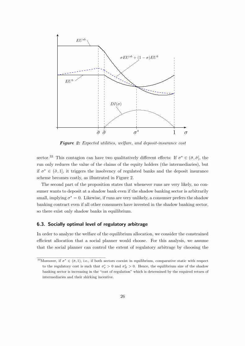
σσ σ 1

DI(σ)

EU b

EUsb

σEUsb + (1− σ)EU b

σ∗

Figure 2: Expected utilities, welfare, and deposit-insurance cost

sector.33 This contagion can have two qualitatively different effects: If σ∗ ∈ (σ, σ], the

run only reduces the value of the claims of the equity holders (the intermediaries), but

if σ∗ ∈ (σ, 1], it triggers the insolvency of regulated banks and the deposit insurance

scheme becomes costly, as illustrated in Figure 2.

The second part of the proposition states that whenever runs are very likely, no con-

sumer wants to deposit at a shadow bank even if the shadow banking sector is arbitrarily

small, implying σ∗ = 0. Likewise, if runs are very unlikely, a consumer prefers the shadow

banking contract even if all other consumers have invested in the shadow banking sector,

so there exist only shadow banks in equilibrium.

6.3. Socially optimal level of regulatory arbitrage

In order to analyze the welfare of the equilibrium allocation, we consider the constrained

efficient allocation that a social planner would choose. For this analysis, we assume

that the social planner can control the extent of regulatory arbitrage by choosing the

33Moreover, if σ∗ ∈ (σ, 1), i.e., if both sectors coexist in equilibrium, comparative static with respect

to the regulatory cost is such that σ∗ρ > 0 and σ∗B > 0. Hence, the equilibrium size of the shadow

banking sector is increasing in the “cost of regulation” which is determined by the required return of

intermediaries and their shirking incentive.

26

composition of the financial system. His only decision variable is the sector size σ, and

we analyze whether the social planner would choose a composition that deviates from

the equilibrium composition σ∗.

The economic trade-off the social planner faces can be illustrated by the following two

extremes: On the one hand, the social planner could choose a banking system in which all

deposits are insured, but regulatory costs imply low interest rates for consumers, σ = 0.

On the other hand, he could choose a banking system in which there is no deposit

insurance and no regulatory cost, σ = 1.34 The social planner chooses an allocation σsp

that trades off the benefit of a deposit insurance and the associated costs of regulation

against the costs of panic-based runs which are a necessity in the presence of disciplining

short-term debt.

We assume that the social planner chooses the composition of the financial system

and thus the degree of regulatory arbitrage in order to maximize the weighted sum of

expected utilities. Formally, his preferred sector size σsp is the solution to the following

problem:

maxσ

(1− σ)EU b(σ) + σEU sb(σ).

By comparing the socially optimal and the equilibrium level of shadow banking, we get

an unambiguous ranking:

Proposition 4. If σ∗ ∈ (σ, 1), it holds that σsp < σ∗.

The proof can be found in the appendix. The proposition states that if the equilibrium

is given by an interior solution, the social planner prefers a shadow banking sector that

is strictly smaller than in a laissez-faire equilibrium. This results from the fact that the

social planner – unlike the agents that are atomistic – internalizes the adverse effects of

increasing σ on the level of expected utility in each sector. As discussed in more detail

in the appendix, the adverse effect of σ via the fire-sale price p can be decomposed into

three components. All three components are internalized by the social planner, but not

by atomistic agents. First, there is the effect of the fire-sale price on the probability

of a run. Second, there is the direct effect of the fire-sale price, i.e., the proceeds of

liquidation in case of a run in the shadow banking sector. Finally, there is the effect on

the cost of the deposit insurance and thus the level of taxation. In addition, there is

the direct effect of σ in determining how many consumers get to enjoy the utility in the

respective sector. While this direct effect is the only locally positive effect of σ, it does

34E.g., this allocation can be compared to the banking system in the US in the 19th century under the

the National Banking Act.

27

not offset the negative effects because, in the constrained efficient allocation, consumers

in both sectors are better off compared to the equilibrium.35

The pecuniary externality has a welfare impact, reminiscent of findings in the literature

on pecuniary externalities in a setup with incomplete markets (compare, e.g., Lorenzoni

(2008)).36 Because regulated banks cannot initially contract the funding conditions

for date 1, a low fire-sale price impacts the overall allocation via deteriorated funding

conditions ex-post. A social planner would internalize this effect, and by limiting the

fire-sale effect, he would also reduce contagion.

Remarkably, however, the social planner would not completely eliminate shadow bank-

ing. He would choose a positive size of the shadow banking sector, σsp > 0, and thus

accept that panic-based runs will occur with a positive probability. E.g., in the example

of Figure 2, he would like to choose the shadow banking sector to be of size σ. The

social planner finds it optimal to utilize the disciplining role of short-term debt. Thus,

it is socially desirable that the shadow banks has a positive size, and the social planner

is willing to accept a positive probability of runs in the shadow banking sector.37 How-

ever, regulatory arbitrage and shadow banking is excessive in equilibrium, and the social

planner would like to contain the adverse consequences of shadow banking that are not

internalized by agents.

7. Policy Implications

In this section, we analyze the effect of government interventions on the equilibrium

composition of the economy. First, we analyze the effect of wholesale funding restrictions,

similar to liquidity regulation in Basel III. Second, we analyze the effect of interventions

by a central bank. Throughout the section, we assume that the extent of regulatory

arbitrage σ is an equilibrium object and cannot be controlled by a social planner.

35The direct effect of σ is locally locally positive if EUsb(σ) > EUb(σ).36Notice, however, that our setup is partial equilibrium and thus general findings in this literature cannot

be applied one-to-one. Nonetheless, the underlying mechanism is similar: agents take the equilibrium

fire-sale price as given.37This is complementary to other arguments why shadow banking may be desirable, such as comparative

advantages in securitizing assets (compare, e.g., Gennaioli et al., 2013; Hanson et al., 2015), or

by relaxing imperfect prudential constraints and utilize self-regulating reputational concerns (see

Ordonez, 2013).

28

7.1. Restrictions on wholesale funding

Given that the contagion of turmoil in the shadow banking sector is due to a deterioration

of funding conditions, limiting the exposure of regulated banks to market conditions

may appear desirable. Can wholesale funding restrictions for regulated banks actually

improve financial stability? For instance, the liquidity regulation in the Third Basel

Accord (Basel III) proposes such restrictions.38 In the following, we analyze a very

simple and extreme case: the complete prohibition of wholesale funding for regulated

banks.

Assumption 5. Regulated banks are required to manage their entire liquidity needs via

storage, i.e., regulated banks face a constraint of L = 0.

Under this constraint, regulated banks can now only offer a contract that is less

attractive than before.

Lemma 4. Assume that regulated banks face capital requirement and wholesale funding

restrictions, and are covered by a deposit insurance scheme. By offering demand-deposit

contracts, they can implement a consumption allocation of

cr1 = R− 1ηR− B

ρ−B (ρ−R)

πR1− 1

η + (1− π)< cb1, and cr2 =

R− Bρ−B (ρ−R)

πR1− 1

η + (1− π)< cb2.

The regulated banking sector cannot experience runs, and it is shielded from adverse

consequences of runs in the shadow banking sector, so the deposit insurance scheme is

costless in equilibrium, i.e. DI(σ) = 0.

Wholesale funding restrictions induce a further allocative inefficiency, as relying on the

liquidity provision by investors allows the generating of higher returns for consumers.39

38Basel III introduces a new assessment and regulation of liquidity risk by defining two minimum stan-

dards of funding liquidity, first described in Basel Committee (2010). The two central measures are

the Liquidity Coverage Ratio (LCR) and the Net Stable Funding Ratio (NSFR). The LCR require-

ment aims to ensure that a bank can withstand a “significantly severe liquidity stress scenario” with

a horizon of 30 days and is described in detail in Basel Committee (2013). It aims to ensure that a

bank has a sufficient stock of liquid assets in order to cover its liquidity needs during the next month.

The objective of the NSFR requirement, elaborated in Basel Committee (2014), is to ensure stable

funding over a one-year horizon. It requires a bank to have an amount of equity, long-term debt, and

other “stable” funding that is sufficient to finance its stock of illiquid assets during the next year.

Taken together, the proposed restrictions act like a restriction on short-term wholesale funding.39The allocation follows from the observation that the consumption allocation under wholesale funding

restrictions coincides with the allocation of Lemma 3 for the case of µ = R, i.e., for the case that

the required return of investors is so high that relying on liquidity provision by investors is equal to

investing in storage. Note that the (cr1, cr2) coincides with the first-best allocation of the Diamond

and Dybvig model if we assume that B = 0 or ρ = R, i.e., if there is no cost of equity.

29

Thus, it holds that

U(cb1, cb2) > U(cr1, c

r2).

However, combined with a deposit insurance scheme, wholesale funding restrictions ac-

tually eliminate the fragility in the banking sector altogether.

We maintain the assumption that shadow banks offer the demand-deposit contract

(csb1 , csb2 ); thus, the equilibrium composition σr in case of wholesale funding restrictions

is determined by the indifference condition

U(cr1, cr2) = EU sb(σr).

As depicted in Figure 3, the equilibrium composition of the financial system changes

unambiguously.

Proposition 5. Introducing wholesale funding restrictions for regulated banks increases

the size of the shadow banking sector, σr > σ∗.

The banking sector becomes less attractive for two reasons: On the one hand, regulated

banks need to hold storage which has a lower return than investing in the productive

asset and managing liquidity needs by relying on wholesale funding. On the other hand,

as banks are not relying on wholesale funding, they will not contribute to the fire sale.

Therefore, shadow banks benefit from the fact that fire sales are less severe and the

fire-sale price is higher, so more consumers will deposit in the shadow banking sector in

equilibrium.

From a social planner’s perspective, this is only desirable if

σrEU sb,r(σr) + (1− σr)EU b,r(σr) ≥ EU∗,

where EU∗ = EU sb(σ∗) = EU b(σ∗) is the level of expected utility that consumers obtain

in equilibrium at both a shadow bank and at a regulated bank in the absence of such

restrictions. Wholesale funding restrictions are desirable if the induced inefficiency in

maturity transformation is less severe than the expected negative effects of the equilib-

rium fire-sale price for the regulated banking sector. In the example of Figure 3, overall

welfare decreases. However, the welfare effect is ambiguous in our model and depends

on how inefficient the use of storage is relative to wholesale funding and how severe the

fire-sale pricing is in equilibrium.

Using our model to take a stand in how the trade-off solves in practice is difficult.

However, the important message of our result is that it is not enough to judge a policy

by its effect on the regulated banking sector alone. It is true that the restrictions

shield the regulated banking sector, and they make their maturity transformation less

30

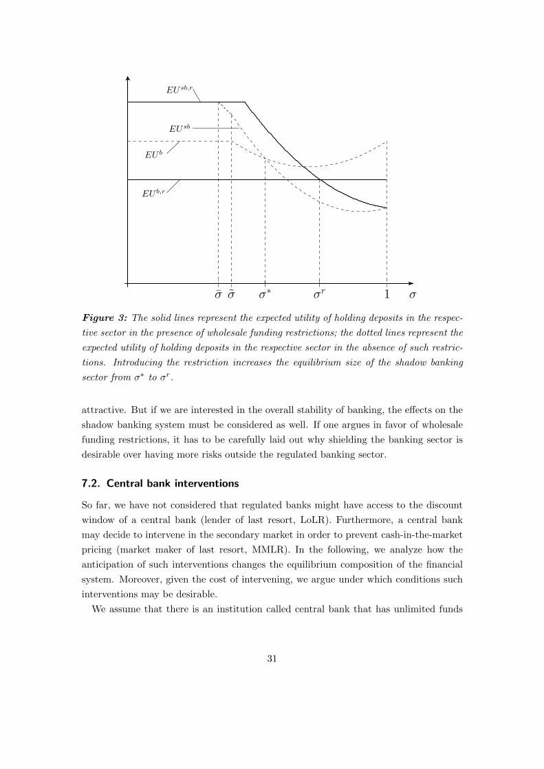
σσ σ 1

EU b,r

EU b

EUsb,r

EUsb

σ∗ σr

Figure 3: The solid lines represent the expected utility of holding deposits in the respec-

tive sector in the presence of wholesale funding restrictions; the dotted lines represent the

expected utility of holding deposits in the respective sector in the absence of such restric-

tions. Introducing the restriction increases the equilibrium size of the shadow banking

sector from σ∗ to σr.

attractive. But if we are interested in the overall stability of banking, the effects on the

shadow banking system must be considered as well. If one argues in favor of wholesale

funding restrictions, it has to be carefully laid out why shielding the banking sector is

desirable over having more risks outside the regulated banking sector.

7.2. Central bank interventions

So far, we have not considered that regulated banks might have access to the discount

window of a central bank (lender of last resort, LoLR). Furthermore, a central bank

may decide to intervene in the secondary market in order to prevent cash-in-the-market

pricing (market maker of last resort, MMLR). In the following, we analyze how the

anticipation of such interventions changes the equilibrium composition of the financial

system. Moreover, given the cost of intervening, we argue under which conditions such

interventions may be desirable.

We assume that there is an institution called central bank that has unlimited funds

31

at its disposal at date 1, and that can commit to being either a LoLR or a MMLR. In a

richer setup that distinguishes between nominal and real values, one could also directly

model the cost of central bank interventions (e.g., political costs, distortions resulting

from inflationary interventions, moral hazard, etc.). As a shortcut, we assume that the

central bank faces a non-pecuniary cost of intervening C(m), where m are the funds that

the central bank needs to use.40

Lender of last resort (LoLR)

We first consider the case that regulated banks have access to the discount window to

borrow funds at the rate that reflects the fundamental value of the regulated banks’

assets.

Assumption 6. The LoLR commits to providing liquidity at date 1 at interest rate

r = µ, and demanding collateral based on the fundamental value R/µ.

The LoLR policy implies that regulated banks do not have to borrow at deteriorated

funding conditions once there is a run in the shadow banking sector. Because regulated

banks face the same terms at the discount window as they do in the market for secured

wholesale funding in normal times, a LOLR policy effectively shields regulated banks

from turmoil in the shadow banking sector. Runs in the shadow banking sector can

still occur, but there is no contagion and the deposit insurance scheme is not tested in

equilibrium.

Surprisingly, shadow banks also benefit from such interventions, although they do

not have access to the discount window. First, shadow bank customers do not face

any taxation to fund the deposit insurance scheme. But second, and more importantly,

because the liquidity need of regulated banks is now satisfied by the central bank, shadow

banks have fewer competitors on the market for liquid funds. In the presence of a LoLR,

the fire-sale price as a function of sector size is given by

pLOLR(σ) =

R/µ if σ ≤ Aµ/R

A/σ if σ > Aµ/R.(11)

40Generally, C(m) might have different shapes. E.g., if there is a high political cost to central bank

interventions, we could have a fixed cost for any positive intervention. If interventions create inflation,

than C(m) should be increasing in m. Moreover, other types of costs may be associated with ex-post

intervention, e.g., if the central bank cannot distinguish between insolvent and illiquid banks or if

interventions give rise to moral hazard. Notice that for both types of intervention policies (LoLR

and MMLR), the central bank is repaid µm units at date 2 if it provides an amount of liquidity m

at date 1. The cost C(m) takes this into account and only measures the net cost of the intervention.

32

The fire-sale price is higher for any composition of the financial system, i.e., pLOLR(σ) >

p(σ) for any σ. This implies, even though both sectors become more attractive for

consumers, that the shadow banking sector becomes relatively more attractive for the

same σ.

Proposition 6. A LoLR policy increases the equilibrium size of the shadow banking

sector, σlolr > σ∗.

The result may appear surprising given that the LoLR policy is exclusively targeted

at regulated banks. Nonetheless, customers of shadow banks benefit equally due to the

weakened fire-sale effects.

Whether the LoLR policy is desirable depends on the shape of C(m). Again, notice

that EU r = EU sb(σlolr) = EU b(σlolr) is the level of expected utility that prevails in

both sectors in an equilibrium with wholesale funding restrictions. If there is a systemic

run on shadow banks, the central bank has to lend an amount of (1 − σlolr)πcb1 to the

regulated banking sector. The equilibrium probability of a run is given by qLOLR =

q(pLOLR(σlolr)). I.e., the expected cost of the central bank intervention is qLOLR(1 −σlolr)πcb1, and the interventions is desirable if

EU r − qLOLRC((1− σlolr)πcb1) ≥ EU∗.

That is, a LoLR intervention improves welfare over the equilibrium allocation if the

direct gains of higher utility in both sectors outweigh the cost of interventions.

It is important to notice that the anticipation of a LoLR policy can increase the

equilibrium probability of a run. Although the fire-sale price under LOLR is higher

for any given composition of the financial system, this effect may be offset by a larger

equilibrium size of the shadow banking sector. Under our assumption that the proba-

bility of runs decreases in the fire-sale price p, the anticipation of the LoLR policy itself

could aggravate systemic risk. This is reminiscent of moral hazard consideration, where

the anticipation of government interventions leads to excessive risk-taking (Acharya and

Yorulmazer, 2008) or excessive maturity mismatch (Farhi and Tirole, 2012). However,

the increased systemic risk is not driven by a moral hazard concern in our model; it is

driven by the changed composition of the financial system.

Market maker of last resort (MMLR)

In contrast to the LoLR’s discount window lending, the MMLR conducts an open market

operation. A MMLR cannot selectively buy assets from regulated banks; it has to buy

assets from all market participants and cannot discriminate.

33

σσ σ 1

EU b,lolr

EU b

EUsb,lolr

EUsb

σ∗σlolr

Figure 4: The solid lines represent the expected utility of holding deposits in the respec-

tive sector in the presence of a LoLR; the dotted lines represent the expected utility of

holding deposits in the respective sector in the absence of a LoLR. The LoLR increases

the equilibrium size of the shadow banking sector from σ∗ to σlolr.

Assumption 7. The Market Maker of Last Resort commits to purchasing the illiquid

assets on the secondary market at price R/µ.

As in the case of the LoLR, regulated banks are unaffected by runs in the shadow

banking sector and the cost of the deposit insurance is reduced to zero. But again, the

shadow banking sector also benefits from the intervention. In fact, the MMLR policy

ensures that the price in the secondary market always remains at p = R/µ, i.e., the

MMLR eliminates cash-in-the-market pricing altogether. Moreover, the central bank

will end up purchasing actual assets whenever there is a run.

Proposition 7. Assume q(p(0)) < q. A MMLR policy completely crowds out regulated

banking, and all intermediation takes place in the shadow banking sector, σmmlr = 1 >

σ∗.

If it is optimal for agents to deposit in the shadow banking sector when no other agent

does so (i.e., if q(p(0)) < q), then it holds that under MMLR policy there will be no

incentive to deposit in the regulated banking sector at all.

34

Whether the MMLR policy is desirable depends again on C(m). Whenever there is a

run, the central bank will have to purchase all assets that are on the market at date 1

at price R/µ. Since only shadow banking prevails in equilibrium, and because they sell

all their assets in a run, the central bank has to use an overall sum of m = R/µ. The

run occurs with probability q(R/µ) = q(p(0)). The expected cost of the central bank

intervention is thus given by q(p(0))C(R/µ). Thus, the MMLR policy is desirable if

q(p(0))C(R/µ) ≤ EU sb − σ∗EU sb + (1− σ∗)EU b.

Again, an intervention is desirable compared to the equilibrium allocation whenever the

expected costs of the intervention are lower than the gains in improving the direct utility

of consumers.

Comparing the LoLR and MMLR policies, it is interesting to notice that under a

MMLR policy, interventions are more likely and larger in extent, i.e.,

q(p(0))C(R/µ) > qLOLRC((1− σlolr)πcb1).

However, the aggregate level of expected utility of consumers is also higher under a

MMLR policy. The desirability of either then depends on the shape of C.

8. Discussion

We develop a model of systemic runs. In contrast to standard bank runs, systemic

runs are contagious and negatively affect other intermediaries by deteriorating their

funding conditions. The underlying mechanism is as follows: Intermediaries manage

their liquidity needs by relying on a market through which investors provide secured

funding. If some intermediaries are subject to a run, they need to liquidate their assets.

Because of a cash-in-the-market constraint, the resulting fire sale can induce a scarcity

of liquid funds in this market and make a run systemic. Here, the reliance on wholesale

funding acts like an endogenous mark-to-market constraint, exposing intermediaries to

changes in asset prices.

We apply the concept of systemic runs in a model in which regulated banks and shadow

banks coexist. Regulated banks are covered by a safety net and are thus immune to

runs. Shadow banks, in contrast, circumvent costly regulatory requirements and thereby

expose themselves to panic-based runs. We derive a number of important implications:

First, cutting contractual linkages between regulated banks and shadow banking entities

may be desirable, but it is insufficient to deal with the financial fragilities emerging

from shadow banking. Turmoil in the shadow banking sector can also be contagious

35

via pecuniary channels, i.e., via markets. Thus, regulatory requirements that prohibit

contractual linkages between the two sectors may be desirable, but of limited efficacy.

Second, the shadow banking sector grows too large in equilibrium as agents do not in-

ternalize their impact on fire-sale prices. While a limited amount of regulatory arbitrage

may be desirable, it is excessive in equilibrium.

Finally, prudential policies as well as central bank interventions change the compo-

sition of the financial system and may ultimately backfire. Strict liquidity regulation,

particularly the prohibition of wholesale funding, is effective in shielding regulated banks

from adverse consequences that originate outside the banking sector. However, this nec-

essarily leads to a larger shadow banking sector, potentially eroding overall financial

stability. Similarly, central bank interventions targeted at reducing fire-sale effects are

more beneficial for the shadow banking sector than they are for regulated banks. Antic-

ipated central bank interventions increase both the likelihood as well as the intensity of

such interventions. This results from a changing composition of the financial sector and

not from standard moral hazard arguments.

36

Appendix A First-Best

We start out with the following first-best maximization program: The first-best maxi-

mization program is given by

max(c1,c2,e0,e2,I,L1,L2)∈R7

+

πu(c1) + (1− π)u(c2), (12)

subject to πc1 ≤ (1 + e0 − I) + L1, (13)

(1− π)c2 ≤ IR− L2 − e2, (14)

e2 ≥ ρe0, (15)

L2 ≥ µL1, (16)

L1 ≤ A, and (17)

I ≤ 1 + e0. (18)

The budget constraints for date one and two are given by (13) and (14). Investors

may transfer L1 to consumers in t = 1 in exchange for L2 units in t = 2. (15) represents

the participation constraint of the intermediary, and (16) represents the participation

constraint of investors. The resource constraint on the investors’ provision of “interim

liquidity” is given by (17), and (18) denotes the constraint on the initial investment.

The two budget constraints are always binding. Furthermore, the participation con-

straint of intermediaries must also be binding. Moreover, e0 > 0 cannot be optimal.

Because ρ > R, we can reduce e0 and thus relax the date-2 constraint. It therefore

follows that e∗0 = e∗2 = 0. Because the intermediaries’ required return is higher than the

asset return, the intermediaries’ funds are not used for intermediation in the first-best.

As we will see below, moral hazard may make it necessary to force the intermediary to

invest some of his endowment.

Let us now turn towards the use of interim liquidity, i.e., wholesale funding at date

1. In the first-best, it also has to hold that the participation constraint of investors is

binding. Whenever L2 < µL1 and L1 ≤ A, we can decrease L2, thereby relaxing the

date-2 constraint. Therefore, it holds that L2 = µL1.

We are now left with a maximization problem with two weak inequalities.

37

max(c1,c2,I,L1)∈R4

+

πu(c1) + (1− π)u(c2), (19)

subject to πc1 = (1− I) + L1, (20)

(1− π)c2 = IR− µL1, (21)

L1 ≤ A, (22)

I ≤ 1. (23)

Let us define the following thresholds:

ξ ≡ µ−1η

πR

(1− π) + πµ1− 1

η

< R/µ, (24)

and

ξ0 ≡πR− 1η

(1− π) + πR− 1ηµ

< ξ, (25)

Depending on the model parameters A,R, µ, and π, as well as on the shape of the

utility function, the first-best program now has three solution candidates.

Lemma 5 (First-best). If A ≥ ξ, then the first-best allocation is characterized by

I∗ = 1 and L∗ = ξµ/R,

and optimal consumption is given by

c∗1 = µ− 1η

R

(1− π) + πµ1− 1

η

and c∗2 =R

(1− π) + πµ1− 1

η

. (26)

For A ∈ (ξ0, ξ), we have that

I∗ = 1, L∗1 = A, and L∗2 = µA, (27)

and optimal consumption is given by

c∗1 =A

πand c∗2 =

R−Aµ(1− π)

. (28)

Finally, if A ≤ ξ0, then the first-best allocation is characterized by

I∗ =(1− π)(1 +A) + πR

− 1ηAµ

(1− π) + πR− 1η

and L∗ = Aµ/R, (29)

and optimal consumption is given by

c∗1 = R− 1ηR+ (R− µ)A

(1− π) + πR− 1η

and c∗2 =R+ (R− µ)A

(1− π) + πR− 1η

. (30)

38

In the first case (A ≥ ξ), it holds that I∗ = 1 and L∗1 < A, and the optimal allocation

is characterized by

u′(c1) = µu′(c2) (31)

πc1µ+ (1− π)c2 = R. (32)

In the third case (A < ξ0), we have L∗1 = A, and I∗ < 1, and the optimal allocation is

characterized by

u′(c1) = Ru′(c2) (33)

πc1R+ (1− π)c2 = R+ (R− µ)A. (34)

Appendix B Financial Markets Implementation

We have by assumption ignored the possibility of implementing an allocation via a

financial market instead of via intermediaries. The allocation that can be attained via

a financial market, i.e., if consumers invest in the technologies directly and trade with

investors in t = 1, is (cfm1 , cfm2 ) = (R/µ,R). This allocation, however, only coincides

with the first-best if η → 1, i.e., if u(c) = ln(c). This is reminiscent of the result of

Diamond and Dybvig (1983).

Nonetheless, we need to make the investment restriction: If we allowed for the co-

existence of financial markets and intermediaries, the incentive to conduct side trading

would destroy the ability to implement the first-best via intermediaries, due to the same

reasoning as in Jacklin (1987) and Farhi et al. (2009). If intermediaries offered the

first-best demand-deposit contract, a consumer would have an incentive to invest his

endowment in the productive technology and to consume the returns R > c∗2 if he turns

out to be patient, or to trade with a patient depositor otherwise, thereby consuming c∗1units.

Appendix C Disciplining Demand Deposits and Shirking

Equilibria

We want to argue that there exists a subgame-perfect Nash equilibrium in which the first-

best consumption profile (c∗1, c∗2) is implemented by the intermediaries offering demand-

deposit contracts that allow consumers to withdraw c∗1 units at t = 1 or c∗2 units at t = 2

and by managing liquidity by relying on investors to provide secured wholesale funding

in t = 1.

39

Observe that in t = 0, intermediaries, due to perfect competition, must offer the best

feasible contract, (c∗1, c∗2), in exchange for the consumers’ endowment. Otherwise, they

would never receive funds in the first place. At date 1, consumers have the possibility

to withdraw the promised amount of c∗1, or to wait until date 2. Importantly, the

intermediaries’ investment decision Ishirk is not observable in t = 0, but becomes publicly

observable before consumers make their withdrawal decision in t = 1.

Consider the following strategy of a consumer for the date-1 subgame: She withdraws

if she turns out to be impatient or if the intermediary has chosen Ishirk > 0, and she does

not withdraw if she turns out to be patient and the intermediary has chosen Ishirk = 0.

We will now show that if all consumers use this strategy, this strategy profile constitutes a

Nash equilibrium of the date-1 subgame for any investment decision of the intermediary,

and the optimal strategy of the intermediary is to choose Ishirk = 0.

Assume that the intermediary has chosen Ishirk > 0. Because all other consumers

withdraw, it is a best response to do so as well because the intermediary is already

illiquid and insolvent in t = 1. Notice further that if Ishirk is large enough, withdrawing

actually becomes a dominant strategy because the intermediary will be illiquid and

insolvent in t = 2 even without a run.

Now assume the intermediary has only invested in the productive technology, i.e.,

I = 1 and Ishirk = 0. Given that only impatient consumers withdraw, the intermediary

will be able to serve all early consumers by selling L∗ units of her investment to investors.

Because A ≥ ξ = πc∗1 by assumption, the investors’ funds are sufficient to serve all early

depositors. As c∗2 > c∗1, it is a best response for patient consumers to wait.

Shirking Equilibria

Note that there also exists a continuum of subgame-perfect Nash equilibria in which the

bank chooses to invest a positive fraction in the shirking technology, but is not disciplined

by the depositors up to this fraction.

There also exist subgame-perfect Nash equilibria in which that short-term debt is

only partially disciplining. In fact, some investment in the shirking technology may

be tolerated by depositors before they run. The reason is that if the intermediary has

chosen some Ishirk ≥ 0 that is small enough, “running” is not the dominant strategy.

Assume the contract (c∗1, c∗2) has been promised. We can ask what level of Ishirk

the intermediary can choose before consumers will run, irrespectively of the behavior

of others at date 1. The date-2 budget constraint in case only impatient consumers

withdraw is given by

(1− π)c2 = (1− Ishirk)R− µL1,

40

where πc∗1 = L1. After observing Ishirk, running is a dominant strategy whenever

c2 =1

1− π[R− Ishirk(R−Rshirk)µπc∗1] < c∗1 (35)

⇔ Ishirk > 1− Rshirk − µπc∗1 − (1− π)c∗1R−Rshirk

≡ Ix. (36)

Therefore, there exist multiple subgame-perfect Nash equilibria in pure strategies

which differ in the extent of the discipline that they ensure. In particular, for any

ψ ∈ [0,min[1, Ix]], there exists an equilibrium in which each consumer runs if and only

if Ishirk > ψ, and intermediaries choose Ishirk = ψ. In the main part of our analysis, we

ignore such equilibria, which is equivalent to assuming that the intermediaries can only

invest in either the productive or the shirking technology, i.e., IShirk ∈ {0, 1}.

Appendix D Optimal Contract with Capital Requirement

Assume a capital requirement is in place as discussed above, i.e.,

e0 =B

ρ−B, e2 = ρe0

Maintaining the assumption that the investors’ capital A is not scarce, the following

constraints are binding:

πc1 = (1 + e0 − I) + Lp,

(1− π)c2 = (I − L)R− e2,

p = R/µ,

I = 1 + e0.

The maximization problem is reduced to

max(c1,c2,L)

πu(c1) + (1− π)u(c2),

subject to πc1 = LR/µ,

(1− π)c2 = (1 + e0 − L)R− ρe0,

e0 =B

ρ−B.

The FOC can be rewritten as

c1 = µ− 1η c2,

41

and the two budget equations yield the following consumption levels:

c1 =RL

πµ, and

c2 =1

1− π

[(1 +

B

ρ−B− L)R− ρ B

ρ−B

].

Solving for c1 and c2 I, and L, we arrive at

I∗∗ = 1 +B

ρ−Band L∗∗ =

πµ1− 1

η

R

R− Bρ−B (ρ−R)

(1− π) + πµ1− 1

η

, (37)

and the optimal consumption is given by

c∗∗1 = µ− 1ηR− B

ρ−B (ρ−R)

(1− π) + πµ1− 1

η

and c∗∗2 =R− B

ρ−B (ρ−R)

(1− π) + πµ1− 1

η

. (38)

Appendix E Liquidity Guarantees

Until this point, we have restricted attention to intermediaries becoming either regulated

banks or unregulated shadow banks. An interesting question is how our results change

when banks and shadow banks are interdependent not only via effects on secondary

markets, but if they are operated by the same intermediary. As described in Section 2,

this had been practice prior to the recent financial crisis, as documented by Acharya

et al. (2013), and has been targeted by post-crisis reforms.

To this end, we analyze a version of our model in which intermediaries operate a

bank and a shadow bank at the same time. We investigate under which conditions

intermediaries may have incentives to use funds from their regulated banking branch to

support their shadow-banking activities in case of distress. We will thus analyze the

effect of explicit contractual linkages.

Private optimality of liquidity guarantees

In the previous section, we assumed that a systemic run on the whole shadow banking

sector is a sunspot phenomenon that occurs with a probability q. We now analyze a sit-

uation in which shadow banks experience idiosyncratic sunspot runs: With a probability

qi, each individual shadow bank experiences a run, and the realization at each shadow

bank is independent of that at other shadow banks. Again we keep the contracts offered

fixed: A commercial bank offers the contract (cb1, cb2), and a shadow bank (csb1 , c

sb2 ).

Given that there is a run on the shadow bank with probability qi, the intermediary

may now have an incentive to guarantee the liquidity of her shadow bank to protect

her from idiosyncratic, i.e., non-systemic, runs. Observe that even in the presence of a

42

coordination device like a sunspot, runs cannot occur if the best response to all other

depositors running is not to run. Thus, idiosyncratic sunspot runs can be eliminated

if a regulated branch of an intermediary provides a credible liquidity guarantee for its

unregulated operations. Moreover, observe that it is optimal to provide this support

guarantee for each institution, as it makes the offered contract more attractive and will

thus attract more consumers.

The liquidity guarantee is credible if the bank can serve all its impatient bank cus-

tomers as well as all those who own a shadow bank contract by selling all its assets.

The regulated banking sector has conducted an initial investment of (1−σ)(1 + e∗0), and

the shadow banking an investment of σ. In total, the bank can thus raise an amount

of liquidity R/γ(1 + (1 − σ)e∗0) at date 1. The funds raised by selling all assets need

to be sufficient to satisfy the claims of all impatient consumers of the regulated bank,

(1− σ)cb1, and of all consumers of the shadow bank, σcsb1 . A liquidity guarantee is thus

credible whenever

σ ≤ R/γ(1 + (1− σ)e∗0)− πcb1csb1 − πcb1

A guarantee can thus only be credible if the shadow banking operations are not too large

compared to the regulated banking activities.

Systemic runs

While it is optimal from the perspective of a single institution to provide a liquidity

guarantee, it leads to an increased parameter space for runs on the aggregate level. In

case of a run, commercial banks have to provide an amount of σcsb1 to shadow banks. In

addition, they require an amount of (1−σ)πcb1 to satisfy their own impatient customers.

Therefore, a run is systemic whenever σcsb1 + (1− σ)πcb1 > A.

Proposition 8. Assume that intermediaries can operate a regulated bank and a shadow

bank at the same time and that liquidity guarantees are credible for the case of idiosyn-

cratic runs. It is privately optimal for each intermediary to guarantee the liquidity for

her shadow bank branch by using funds from her regulated bank. In turn, this decreases

the threshold size above which the shadow banking sector becomes systemic: A systemic

run can occur and affect regulated banks if σ ≥ σguar, where

σguar =A− πcb1csb1 − πcb1

< σ.

Without liquidity guarantees, systemic runs are only possible if the shadow banking

sector’s size exceeds σ. With liquidity guarantees, this is already true for a sector size

43

of σ ≥ σguar < σ. The underlying mechanism is as follows: while liquidity guarantees

are optimal from the individual intermediary’s perspective, they increase the number of

assets sold in case of a systemic run in the shadow banking sector. This shows that there

is a clear benefit of preventing direct contractual linkages via regulation, as it reduces

the parameter space in which systemic runs may take place. However, as shown in the

earlier section, it may not be sufficient to rule out adverse effect for regulated banks

entirely.

Appendix F Optimal Contracts with Sunspot-Induced Runs

If runs on shadow banks occur with a probability q(p(σ)), then the optimal contracts

depend on the sector size σ directly through the fire-sale price and indirectly through

the probability of sunspots. In order to solve the problem, we switch the setup slightly

and assume that the cost of deposit insurance is not subtracted from the consumption

levels, but rather enters additively separable with the functional form v(DI(σ)), where

v is strictly increasing and twice continuously differentiable.

Regulated Banks

The only change in the problem of regulated banks is that the cost of equity is increasing

in q. We can distinguish three cases: First, if σ is so low such that p(σ) = R/µ, banks

offer the old contract. Second, for a small range of σs, the equity is partly wiped out in

a run. Third, the equity is completely wiped out in case of a systemic run.

Given that the bank equity is wiped out with some probability q, the equity holders’

promised rate of return has to be increased to ρ/(1− q) in order to reimburse them for

the default risk. That is, we have that e2 = ρ1−qe0 and e0 = B

ρ/(1−q)−B .

max(c1,c2,L)∈R3

+

πu(c1) + (1− π)u(c2)]− (1− q(p(σ)))v(DI(σ)),

subject to πc1 = LR/µ,

(1− π)c2 = (1 + e0 − L)R− ρe0,

e0 =B

ρ/(1− q)−B.

The bank thus offers a contract with

cb1(q) = µ− 1η

R− Bρ/(1−q)−B (ρ/(1− q)−R)

(1− π) + πµ1− 1

η

and cb2(q) =R− B

ρ/(1−q)−B (ρ/(1− q)−R)

(1− π) + πµ1− 1

η

.

(39)

It holds that cb1(q) and cb2(q) are decreasing in q.

44

Shadow Banks

The optimization problem for shadow banks changes as shadow banks may desire to

invest in storage. The expected utility in the shadow banking sector is given by

EU sb(c1, c2, I|σ) = (1−q(p))[πu(c1)+(1−π)u(c2)]+q(p(σ))[u(1+I(p(σ)−1))−v(DI(σ))].

The optimization problem for a representative shadow bank is:

maxc1,c2,I,L

EU sb(c1, c2, I|σ)

subject to πc1 = 1− I + L1,

(1− π)c2 = IR− µL1,

I ≤ 1.

We first substitute for c2 and fix I, then we can solve for the optimal “response

function” c∗1(I). We yield a function EU sb(I, c∗1(I)|σ), and we take the total derivative

wrt. I and evaluate it at I = 1. If this is positive, then I∗ = 1.

It is clear that in the good state (no run), I has an unambiguously positive effect;

it increases consumption at both dates. In the bad state (run), the effect is negative

if p(σ) < 1. However, the positive effect outweighs the negative effect as long as the

probability of a run is sufficiently small.

EU sb(c1, I|σ) =(1− q(p))[πu(c1) + (1− π)u

(IR− µ(πc1 − 1− I)

1− π

)]+ q(p(σ))[u(1 + I(p(σ)− 1))− v(DI(σ))].

As usual, optimality requires that c∗1(I) satisfies the FOC u′(c1) = µu′(c2). We obtain

the consumption level functions

c∗1(I) = µ− 1η

I(R− 1) + 1

(1− π) + πµ1− 1

η

, and c∗2(I) =I(R− 1) + 1

(1− π) + πµ1− 1

η

.

The total derivative of the expected utility is given by

dEU sb(c1, I|σ)

dI=(1− q(p))R− I

1− π

[πµ− 1η u′(c∗1(I)) + (1− π)u′(c∗2(I))

]︸ ︷︷ ︸

>0

+ q(p(σ)) (p(σ)− 1)u′(1 + I(p(σ)− 1))︸ ︷︷ ︸<0 if p(σ)<1

.

45

Appendix G Proof of Proposition 3

We want to show that there exists q and q such that for q(p(1)) > q and q(p(0)) < q, it

holds that

σ∗ ∈ (σ, 1).

Moreover, whenever q(p(1)) ≤ q, it holds that σ∗ = 1, and there are only shadow banks;

whenever q(p(0)) ≥ q, it holds that σ∗ = 0, and there are only regulated banks.

Proof. We first analyze the second part of the proposition. For σ = 1 to be an equilib-

rium, it must hold that

EU b(1) < EU sb(1)

Observe that at σ = 1 it holds that DI(1) = 0 and EU b(1) = qU(csb1 , csb2 )+(1−q)u(p(1))

and EU b(1) = U(cb1cb2). Thus, in order for EU b(1) < EU sb(1) to hold, we must have

that given all parameters:

q =U(csb1 , c

sb2 )− U(cb1c

b2)

U(csb1 , csb2 )− U(cb1c

b2) + U(cb1, c

b2)− u(p(1))

.

Likewise, for σ = 0 to be an equilibrium, it must hold that

EU b(0) > EU sb(0)

Again, we have that σ = 0 implies that DI(0) = 0 and EU b(1) = (1 − q)U(csb1 , csb2 ) +

qu(R/µ) and EU b(1) = U(cb1cb2). Thus in order for EU b(0) > EU sb(0) to hold, we must

have that given all parameters:

q =U(csb1 , c

sb2 )− U(cb1c

b2)

U(csb1 , csb2 )− u(R/µ)

Finally, observe that EU sb(0) = EU sb(σ) by definition. Therefore, whenever q(p(1)) >

q and q(p(0)) < q, it holds that

σ∗ ∈ (σ, 1).

Appendix H Proof of Proposition 4

Proof. Approach: Show that for all σ /∈ [σ, σ∗), it holds that W (σ) < W (σ).

Step 1a: Show that W (σ) < W (σ) for all σ > σ∗

Step 1b: Show that W (σ) < W (σ) for all σ < σ

46

Step 2: Show that W (σ∗) < W (σ)

It holds that

EU b(σ∗) < EU b(σ)

EU sb(σ∗) < EU sb(σ)

Welfare

W (σ∗) = (1− σ∗)EU b(σ∗) + σ∗EU sb(σ∗)

< (1− σ∗)EU b(σ) + σ∗EU sb(σ)

< (1− σ)EU b(σ) + σEU sb(σ)

= W (σ)

Step 3: It has to hold that σsp ∈ [σ, σ∗).

Remarks:

If σ∗ = 1, then σsp ≤ σ∗ = 1.

If σ∗ = 0, then σsp = σ∗ = 0.

σ∗ ∈ (0, σ] can only prevail if EU sb(0) < EU sb(0). In this case, all σ ∈ (0, σ] constitute

an equilibrium, and the social planner is indifferent between all of these.

In order to gain deeper understanding of what it is that the social planner can do that

agents cannot, we can analyze the corresponding FOC, which implies that σSP satisfies

EU b(σ)

EU sb(σ)= 1 + ∆(σ)

in an interior solution to the problem, and where ∆(σ) is given by

∆(σ) =1

EU sb(σ)q(p(σ))

·

[σ

[q′(p(σ))p′(σ)(U sb(σ)− U(csb1 , c

sb2 ))︸ ︷︷ ︸

Extensive margin shadow banks

+ u′(p(σ)−DI(σ))[p′(σ)−DI ′(σ)]︸ ︷︷ ︸Intensive margin shadow banks

]

+ (1− σ)

[q′(p(σ))p′(σ)(U b(σ)− U(cb1, c

b2))︸ ︷︷ ︸

Extensive margin banks

+ U bσ(σ)︸ ︷︷ ︸Intensive margin banks

]],

47

and U sb(σ) = u(p(σ)−DI(σ)) and U b(σ) = U(cb1−DI(σ), cb2−DI(σ)) denote the utility

in the two sectors in case of a run, and U bσ(σ) and U sbσ (σ) the respective derivatives with

respect to σ.

Recall, in equilibrium, if the two sector coexists, σ∗ is such that

EU b(σ)

EU sb(σ)= 1.

That is, the difference between the equilibrium and the social planner’s preferred allo-

cation is captured in ∆(σ). ∆ can be decomposed into three different components that

the social planner internalizes, but agents do not. First, the social planner internalizes

the effect of σ via the fire-sale price on an increased probability of sunspots q, referred

to as the extensive margin effect. Second, he internalizes the effect of σ directly on

the fire-sale price and thus the proceeds in case of a run in the shadow banking sector.

Finally, he internalizes the effect of σ via the fire-sale price on the cost of the deposit

insurance and thus the level of taxation across all agents. The latter two effects can be

referred to as the intensive margin.

48

References

Acharya, Viral, Thomas Philippon, Matthew Richardson, and Nouriel Roubini (2009).

“Prologue: A Bird’s Eye View. The Financial Crisis of 2007-2009: Causes and Reme-

dies”. Financial Markets, Institutions & Instruments 18, 89–137.

Acharya, Viral V., and Tanju Yorulmazer (2007). “Too Many to Fail – An Analysis of

Time-Inconsistency in Bank Closure Policies”. Journal of Financial Intermediation

16, 1–31.

(2008). “Cash-in-the-Market Pricing and Optimal Resolution of Bank Failures”.

Review of Financial Studies 21, 2705–2742.

Acharya, Viral V., Philipp Schnabl, and Gustavo A. Suarez (2013). “Securitization with-

out Risk Transfer”. Journal of Financial Economics 107, 515–536.

Admati, Anat, Peter DeMarzo, Paul Pfleiderer, and Martin Hellwig (2013). “The Lever-

age Ratchet Effect”. Preprints of the Max Planck Insitute for Research on Collective

Goods.

Adrian, Tobias, and Hyun Song Shin (2011). “Financial Intermediary Balance Sheet

Management”. Annual Review of Financial Economics 3, 289–307.

(2014). “Procyclical Leverage and Value-at-Risk”. Review of Financial Studies

27, 373–403.

Allen, Franklin, and Douglas Gale (1994). “Limited Market Participation and Volatility

of Asset Prices”. American Economic Review 84, 933–955.

(1998). “Optimal Financial Crises”. The Journal of Finance LIII, 1245–1284.

(2000). “Financial Contagion”. Journal of Political Economy 108, 1–33.

(2007). Understanding Financial Crises. Oxford: Oxford University Press.

Basel Committee – Basel Committee on Banking Supervision (2010). Basel III: Inter-

national Framework for Liquidity Risk Measurement, Standards and Monitoring.

Basel: Bank for International Settlement.

Basel Committee – (2013). Basel III: The Liquidity Coverage Ratio and Liquidity

Risk Monitoring Tools. Basel: Bank for International Settlement.

Basel Committee – (2014). Basel III: The Net Stable Funding Ratio. Basel: Bank

for International Settlement.

Bengui, Julien, and Javier Bianchi (2014). “Capital Flow Management when Capital

Controls Leak”. Mimeo.

Bhattacharya, Sudipto, and Douglas Gale (1987). “Preference Shocks, Liquidity and

Central Bank Policy”. In: New Approaches to Monetary Economics, Cambridge

University Press, ed. by W. Barnett, and K. Singleton. Cambridge University Press,

69–89.

49

Bolton, Patrick, Tano Santos, and Jose A. Scheinkman (2011). “Outside and Inside

Liquidity”. Quarterly Journal of Economics 126, 259–321.

Brunnermeier, Markus K. (2009). “Deciphering the Liquidity and Credit Crunch 2007-

2008”. Journal of Economic Perspectives 23, 77–100.

Bryant, John (1980). “A Model of Reserves, Bank Runs, and Deposit Insurance”. Journal

of Banking & Finance 4, 335–344.

Calomiris, Charles, and Charles Kahn (1991). “The Role of Demandable Debt in Struc-

turing Optimal Banking Arrangements”. American Economic Review 81, 497–513.

Cetorelli, Nicola (2014). “Hybrid Intermediaries”. NY FED Staff Report.

Chari, VV, and Ravi Jagannathan (1988). “Banking Panics, Information, and Rational

Expectations Equilibrium”. The Journal of Finance XVIII, 749–761.

Claessens, Stijn, and Lev Ratnovski (2014). “What is Shadow Banking?” IMF Working

Paper 14/25.

Cooper, Russell, and Thomas W. Ross (1998). “Bank runs: Liquidity Costs and Invest-

ment Distortions”. Journal of Monetary Economics 41, 27–38.

Copeland, Adam, Antoine Martin, and Michael Walker (2014). “Repo Runs: Evidence

from the Tri-Party Repo Market”. The Journal of Finance LXIX, 2343–2380.

Covitz, Daniel, Nellie Liang, and Gustavo A. Suarez (2013). “The Evolution of a Finan-

cial Crisis: Panic in the Asset-Backed Commercial Paper Market”. The Journal of

Finance LXVII, 815–847.

Diamond, Douglas W., and Philip H. Dybvig (1983). “Bank Runs, Deposit Insurance,

and Liquidity”. Journal of Political Economy 91, 401–419.

Diamond, Douglas W., and Raghuram G. Rajan (2001). “Liquidity Risk, Liquidity Cre-

ation and Financial Fragility: A Theory of Banking”. Journal of Political Economy

109, 287–327.

(2005). “Liquidity Shortages and Banking Crises”. The Journal of Finance XI,

615–647.

(2011). “Fear of Fire Sales, Illiquidity Seeking, and Credit Freezes”. The Quar-

terly Journal of Economics 126, 557–591.

European Central Bank (2014). Banking Structures Report. Frankfurt: European Central

Bank.

Farboodi, Maryam (2015). “Intermediation and Voluntary Exposure to Counterparty

Risk”. Working Paper, 1–66.

Farhi, Emmanuel, and Jean Tirole (2012). “Collective Moral Hazard, Maturity Mismatch

and Systemic Bailouts”. American Economic Review 102, 60–93.

50

Farhi, Emmanuel, Mikhail Golosov, and Aleh Tsyvinski (2009). “A Theory of Liquidity

and Regulation of Financial Intermediation”. Review of Economic Studies 76, 973–

992.

Financial Crisis Inquiry Commission (2011). The Financial Crisis Inquiry Report. Wash-

ington D.C.: Printing Office of the US Government.

FSB – Financial Stability Board (2013). Global Shadow Banking Monitoring Report 2013.

Basel: Bank for International Settlement.

FSB – (2014). Global Shadow Banking Monitoring Report 2014. Basel: Bank for

International Settlement.

Freixas, Xavier, Bruno M. Parigi, and Jean-Charles Rochet (2000). “Systemic Risk,

Interbank Relations, and Liquidity Provision by the Central Bank”. Journal of

Money, Credit and Banking 32, 611–638.

Gennaioli, Nicola, Andrei Shleifer, and Robert W. Vishny (2013). “A Model of Shadow

Banking”. The Journal of Finance LXVIII, 1331–1363.

Gertler, Mark, and Nobuhiro Kiyotaki (2015). “Banking, Liquidity and Bank Runs in

an Infinite-Horizon Economy”. American Economic Review 105, 2011–2043.

Goldstein, Itay, and Ady Pauzner (2005). “Demand-Deposit Contracts and the Proba-

bility of Bank Runs”. The Journal of Finance LX, 1293–1327.

Gorton, Gary B., and Andrew Metrick (2012). “Securitized Banking and the Run on

Repo”. Journal of Financial Economics 104, 425–451.

Greenwood, Robin, Augustin Landier, and David Thesmar (2015). “Vulnerable banks”.

Journal of Financial Economics 115, 471–485.

Hakenes, Hendrik, and Isabel Schnabel (2015). “Separating Trading and Banking: Con-

sequences for Financial Stability”. Working Paper.

Hanson, Samuel G., Andrei Shleifer, Jeremy C. Stein, and Robert W. Vishny (2015).

“Banks as Patient Fixed-Income Investors”. Journal of Financial Economics 117,

449–469.

He, Zhiguo, and Wei Xiong (2012). “Dynamic Debt Runs”. Review of Financial Studies

25, 1799–1843.

Hellwig, Martin F. (1994). “Liquidity Provision, Banking, and the Allocation of Interest

Rate Risk”. European Economic Review 38, 1363–1389.

(2009). “Systemic Risk in the Financial Sector: An Analysis of the Subprime-

Mortgage Financial Crisis”. De Economist 157, 129–207.

Holmstrom, Bengt, and Jean Tirole (1998). “Private and Public Supply of Liquidity”.

Journal of Political Economy 106, 1–40.

51

Holmstrom, Bengt, and Jean Tirole (2011). Inside and Outside Liquidity. Cambridge,

MA: The MIT Press.

Huang, Ji (2014). “Banking and Shadow Banking”. Working Paper.

International Monetary Fund (2013). “Changes in Bank Funding Patterns and Finan-

cial Stability Risks”. Global Financial Stability Report: Transition Challenges to

Stability, 105–148.

(2015). “The Asset Management Industry And Financial Stability”. Global Fi-

nancial Stability Report: Transition Challenges to Stability, 93–135.

Jacklin, Charles J. (1987). “Demand Deposits, Trading Restrictions, and Risk Sharing”.

In: Contractual Arrangements for Intertemporal Trade. Ed. by Edward C. Prescott,

and Neil Wallace. University of Minnesota Press, 26–47.

Jacklin, Charles J., and Sudipto Bhattacharya (1988). “Distinguishing Panics and Information-

based Bank Runs: Welfare and Policy Implications”. Journal of Political Economy

96, 568–592.

Jones, David (2000). “Emerging Problems with the Basel Capital Accord: Regulatory

Capital Arbitrage and Related Issues”. Journal of Banking & Finance 24, 35–58.

Kacperczyk, Marcin, and Philipp Schnabl (2009). “When Safe Proved Risky: Commercial

Paper during the Financial Crisis of 2007-2009”. Journal of Economic Perspectives

24, 29–50.

Krishnamurthy, Arvind, Stefan Nagel, and Dmitry Orlov (2014). “Sizing Up Repo”. The

Journal of Finance LXIX, 2381–2417.

Lorenzoni, Guido (2008). “Inefficient Credit Boom”. The Review of Economic Studies

75, 809–833.

Luck, Stephan, and Paul Schempp (2014a). “Banks, Shadow Banking, and Fragility”.

ECB Working Paper No 1726.

(2014b). “Outside Liquidity, Rollover Risk, and Government Bonds”. Preprint

of the Max Planck Institute for Research on Collective Goods Bonn No. 2014/14.

Martin, Antoine, David Skeie, and Ernst Ludwig Von Thadden (2014a). “Repo Runs”.

Review of Financial Studies 27, 957–989.

(2014b). “The Fragility of Short-Term Secured Funding Markets”. Journal of

Economic Theory 149, 15–42.

Morris, Stephen, and Hyun Song Shin (1998). “Unique Equilibrium in a Model of Self-

Fufilling Currency Attacks”. American Economic Review 88, 12.

(2003). “Global Games: Theory and Applications”. In: Advances in Economics

and Econometrics (Proceedings of the Eighth World Congress of the Econometric

52

Society). Ed. by M. Dewatripont, L. Hansen, and S. Turnoyvsky. Vol. 35. Cambridge

University Press, 56–114.

Morris, Stephen, and Hyun Song Shin (2010). “Illiquidity Component of Credit Risk”.

Working Paper, 1–44.

Myers, Stewart C., and Nicholas S. Majluf (1984). “Corporate Financing and Investment

Decisions when Firms have Information that Investors do Not Have”. Journal of

Financial Economics 13, 187–221.

Ordonez, Guillermo (2013). “Sustainable Shadow Banking”. NBER Working Paper No.

19022.

Postlewaite, Andrew, and Xavier Vives (1987). “Bank Runs as an Equilibrium Phe-

nomenon”. Journal of Political Economy 95, 485.

Pozsar, Zoltan, Tobias Adrian, Adam Ashcraft, and Hayley Boesky (2013). “Shadow

Banking”. Federal Reserve Bank of New York Economic Policy Review, 1–16.

Qi, Jianping (1994). “Bank Liquidity and Stability in an Overlapping Generations Model”.

Review of Financial Studies 7, 389–417.

Rochet, Jean-Charles, and Xavier Vives (2004). “Coordination Failures and the Lender

of Last Resort: Was Bagehot Right After All?” Journal of the European Economic

Association 2, 1116–1147.

Schmidt, Lawrence, Allan Timmermann, and Russ R. Wermers (2014). “Runs on Money

Market Mutual Funds”. Working Paper.

Segura, Anatoli (2014). “Why did Sponsor Banks Rescue their SIVs? A Signaling Model

of Rescues”. Working Paper.

Shleifer, Andrei, and Robert W. Vishny (1997). “The Limits of Arbitrage”. The Journal

of Finance LII, 35–55.

Skeie, David R. (2008). “Banking with Nominal Deposits and Inside Money”. Journal

of Financial Intermediation 17, 562–584.

Uhlig, Harald (2010). “A Model of a Systemic Bank Run”. Journal of Monetary Eco-

nomics 57, 78–96.

Wallace, Neil (1988). “Another Attempt to Explain an Illiquid Banking System: The Di-

amond and Dybvig Model with Sequential Service Taken Seriously”. Federal Reserve

Bank of Minneapolis Quarterly Review Fall, 3–16.

53