regulatory impact analysis for the stationary spark ... · stationary si engines. by model year...

Regulatory Impact Analysis for the Stationary Spark-Ignition New Source Performance Standard (SI NSPS) and New Area Source NESHAP

December 2007

EPA-452/R-07-015

Regulatory Impact Analysis for the Stationary Spark Ignition New Source Performance

Standard (SI NSPS) and New Area Source NESHAP

Prepared for

U.S. Environmental Protection Agency

Office of Air Quality Planning and Standards (OAQPS) Air Benefit and Cost Group (ABCG) Research Triangle Park, NC 27711

Prepared by

RTI International 3040 Cornwallis Road

Research Triangle Park, NC 27709

CONTENTS

Section Page

1. Introduction................................................................................................................... 1-1

1.1 Executive Summary ............................................................................................. 1-1

1.2 Reason for Today’s Action .................................................................................. 1-2 1.2.1 Market Failure or Other Social Purpose .................................................. 1-2

1.3 Organization of this Report.................................................................................. 1-4

2. Industry Profile ............................................................................................................. 2-1

2.1 The Supply Side................................................................................................... 2-1 2.1.1 Equipment Production Costs ................................................................... 2-1

2.2 The Demand Side................................................................................................. 2-6 2.2.1 Generators and Welding Equipment........................................................ 2-6 2.2.2 Stationary Pumps and Compressor Equipment...................................... 2-10 2.2.3 Irrigation ................................................................................................ 2-11

2.3 Industry Organization ........................................................................................ 2-13 2.3.1 Engines: The Equipment Firm’s “Make” or “Buy” Decision................ 2-13 2.3.2 Distribution of Small and Large Firms .................................................. 2-14

2.4 Historical Market Data....................................................................................... 2-15 2.4.1 Price Trends ........................................................................................... 2-19

2.5 Projections.......................................................................................................... 2-19

3. Costs, Economic Impact Analysis, and Emissions ....................................................... 3-1

3.1 Cost Estimate Background................................................................................... 3-1

3.2 Regulatory Program Cost Estimates .................................................................... 3-1

3.3 Economic Framework.......................................................................................... 3-3

iii

3.4 Conclusion for Economic Impacts....................................................................... 3-4 3.5 Baseline Emissions and Emission Reductions………………………………….3-5

4. Energy Impacts ............................................................................................................. 4-1

5. Small Business Impact Analysis................................................................................... 5-1

5.1 Description of Small Entities Affected ................................................................ 5-1

5.2 Small Business Screening Analysis ..................................................................... 5-1

5.3 Assessment Results and Conclusions .................................................................. 5-3

6. Human Health Benefits of Emissions Reductions ........................................................ 6-1

6.1 Calculation of Human Health Benefits ................................................................ 6-1

6.2 Characterization of Uncertainty in the Benefits Estimates .................................. 6-2

6.3 Monte Carlo–Based Uncertainty Analysis........................................................... 6-5

6.4 Updating the Benefits Data Underlying the Benefit per Ton Estimates.............. 6-7

6.5 Comparison of Benefits and Costs....................................................................... 6-7

References.....................................................................................................................R-1

iv

LIST OF FIGURES

Number Page

2-1. Trends in Marginal Oil and Gas Production: 1996 to 2005........................................ 2-12 2-2. Engine Companies’ Employment Distribution, 2005 (N = 21) .................................. 2-16 2-3. Engine Companies’ Sales Distribution (N = 21) ........................................................ 2-16 2-4. Equipment Companies’ Employment Distribution, 2005 (N = 60)............................ 2-17 2-5. Equipment Companies’ Sales Distribution (N = 60) .................................................. 2-17 2-6. Price Trends for Equipment and Engines ................................................................... 2-19 3-1. Long Run: Full-Cost Pass-Through.............................................................................. 3-4

v

LIST OF TABLES

Number Page

2-1. Motor and Generator Manufacturing: 2005 and Earlier Years ($billion)..................... 2-3 2-2. Welding and Soldering Equipment Manufacturing: 2002 and Earlier Years

($billion) ....................................................................................................................... 2-4 2-3. Pumps and Pumping Equipment Manufacturing: 2005 and Earlier Years

($billion) ....................................................................................................................... 2-5 2-4. Air and Gas Compressor Manufacturing: 2005 and Earlier Years ($billion) ............... 2-7 2-5. Farm Machinery and Equipment Manufacturing: 2005 and Earlier Years

($billion) ....................................................................................................................... 2-8 2-6. Generator Set and Welding Equipment Use by Industry: 1997.................................... 2-9 2-7. Pumps and Compressor Equipment Use by Industry: 1997 ....................................... 2-10 2-8. Reported Gross Revenue Estimates from Marginal Wells: 2005 ............................... 2-11 2-9. Expenses per Acre by Type of Energy: 2003 (dollars)............................................... 2-13 2-10. Number of On-Farm Pumps of Irrigation Water by Type of Energy: 1998 and

2003............................................................................................................................. 2-13 2-11. Distribution of Engine and Equipment Production by Business Size: 2002 and

Earlier Years ............................................................................................................... 2-15 2-12. Estimated Historical Unit Sales Data by Market: 1998–2002 .................................... 2-18 2-13. Projected Unit Sales Data by Horsepower Range: Selected Years............................. 2-20 3-1. Average Total Cost per Engine: 2015 (2005$) ............................................................. 3-2 3-2. Comparison of Regulatory Program Costs and Value of Shipments: 2015.................. 3-3 3-3. Baseline Emissions in 2015 by Engine Size Category ................................................. 3-5 3-4. Emission Reductions in 2015 by Engine Size Category............................................... 3-6

4-1. Affected Industry Share by Fuel Type: 2015................................................................ 4-2 5-1. Summary Statistics for SBREFA Screening Analysis.................................................. 5-3 6-1. Estimate of Monetized Benefits by 2015 ($2005) ........................................................ 6-2

vi

SECTION 1 INTRODUCTION

The U.S. Environmental Protection Agency (EPA) proposed a New Source Performance Standard (NSPS) on spark ignition (SI) stationary internal combustion engines in May 2006 and will promulgate this rule by December 20, 2007. This rule, which is in response to a settlement agreement and is under the authority of section 111(b) of the Clean Air Act, will address emissions for nitrogen oxides (NOx), particulate matter (PM), and carbon monoxide (CO) from new SI engines. The NSPS contains requirements for owners, operators, and manufacturers of stationary SI engines. By model year 2015, 411 stationary SI engines must be certified to the final Tier 4 emission standards for all pollutants. In addition, EPA proposed simultaneously a national standard to address hazardous air pollutant (NESHAP) emissions from existing and new stationary SI engines. These rules together are considered “economically significant” according to Executive Order 12866 because the benefits and costs together for these rules are likely to exceed $100 million.

Because of the effect of a recent DC Circuit Court of Appeals decision on the legality of another NESHAP, EPA has decided not to promulgate a standard to address HAP emissions from existing stationary SI engines by December 2007. HAP emissions from those engines will be addressed in a separate rulemaking that will take place after December 20, 2007. The stationary SI NSPS and new area source NESHAP will be promulgated by December 20, 2007, as currently planned.

As part of the regulatory process of preparing these standards EPA is required to develop a regulatory impact analysis (RIA). This RIA includes an economic impact analysis (EIA), a small entity impacts analysis and a benefits analysis for the final rule to be promulgated in December, 2007. This report documents the methods and results of this RIA.

1.1 Executive Summary

The key results of the RIA are as follows:

Engineering Cost Analysis: EPA estimates total annualized costs of the NSPS will be $18.6 million for the year 2015. The total annualized costs associated with the NESHAP for 250 to 500 hp 4-stroke lean burn (4SLB) SI engines located at major sources will be $3.1 million for the year 2015. Both programs together yield an annualized cost of approximately $21.7 million (2005$).

Market Analysis: The average total cost data per engine suggest percentage changes in affected engine prices may range from 5% to 33%. Although these changes are

1-1

large, economic theory and other EPA economic models of engine markets suggest demand for engines is inelastic and changes in consumption are likely to be small.

Economic Welfare Analysis: EPA believes the national annualized compliance cost estimates provide a reasonable approximation of the social cost of this regulatory program. The engineering analysis estimated annualized costs of $21.7 million in 2015.

Energy Impacts: EPA concludes that the rule when implemented will not have a significant adverse effect on the supply, distribution, or use of energy.

Small Business Analysis: EPA performed a screening analysis for impacts on small businesses by comparing compliance costs to average company revenues. EPA’s analysis found that the ratio of compliance cost to company revenue falls below 1% for four of the five small companies included in the screening analysis. In addition, the average cost to sales for companies in industries affected by this rule is 0.10% and lower. One small firm would have an annualized cost of more than 1% of sales associated with meeting the requirements; the estimated cost is 5% of sales for this small firm. No other adverse impacts are expected to these affected small businesses.

Benefits Analysis: EPA estimates that the monetized benefits of this rule are $220 million (2005$), which exceeds the estimated annualized engineering or social costs of $21.7 million. Thus, the monetized benefits of this rule exceed the costs by about $200 million (2005$). EPA recognizes the uncertainty associated with this estimate and readers may refer to the benefits chapter in this RIA for a discussion of the range of benefits estimated for this rule.

1.2 Reason for Today’s Action

1.2.1 Market Failure or Other Social Purpose

The stationary SI NSPS and NESHAP is of sufficient impact to fall under the requirements for Executive Order 12866 as amended in January 2007 (OMB, 2007). Among the reasons a regulation such as this one may be issued is to address market failure. The major types of market failure include externality, market power, and inadequate or asymmetric information. Correcting market failures is a reason for regulation, but it is not the only reason. Other possible justifications include improving the functioning of government, removing distributional unfairness, or promoting privacy and personal freedom.

Externality, Common Property Resource, and Public Good

An externality occurs when one party’s actions impose uncompensated benefits or costs on another party. Environmental problems are a classic case of externality. For example, the smoke from a factory may adversely affect the health of local residents while soiling the property in nearby neighborhoods. If bargaining were costless and all property rights were well defined, people would eliminate externalities through bargaining without the need for government

1-2

regulation. From this perspective, externalities arise from high transactions costs and/or poorly defined property rights that prevent people from reaching efficient outcomes through market transactions.

Resources that may become congested or overused, such as fisheries or the broadcast spectrum, represent common property resources. “Public goods,” such as defense or basic scientific research, are goods where provision of the good to some individuals cannot occur without providing the same level of benefits free of charge to other individuals.

Market Power

Firms exercise market power when they reduce output below what would be offered in a competitive industry to obtain higher prices. They may exercise market power collectively or unilaterally. Government action can be a source of market power, such as when regulatory actions exclude low-cost imports. Generally, regulations that increase market power for selected entities should be avoided. However, there are some circumstances in which government may choose to validate a monopoly. If a market can be served at lowest cost only when production is limited to a single producer (local gas and electricity distribution services, for example) a natural monopoly is said to exist. In such cases, the government may choose to approve the monopoly and to regulate its prices and/or production decisions. Nevertheless, analysts should keep in mind that technological advances often affect economies of scale. This can, in turn, transform what was once considered a natural monopoly into a market where competition can flourish.

Inadequate or Asymmetric Information

Market failures may also result from inadequate or asymmetric information. Because information, like other goods, is costly to produce and disseminate, an evaluation will need to do more than demonstrate the possible existence of incomplete or asymmetric information. Even though the market may supply less than the full amount of information, the amount it does supply may be reasonably adequate and therefore not require government regulation. Sellers have an incentive to provide information through advertising that can increase sales by highlighting distinctive characteristics of their products. Buyers may also obtain reasonably adequate information about product characteristics through other channels, such as a seller offering a warranty or a third party providing information.

Even when adequate information is available, people can make mistakes by processing it poorly. Poor information processing often occurs in cases of low-probability, high-consequence events, but it is not limited to such situations. For instance, people sometimes rely on mental rules of thumb that produce errors. If they have a clear mental image of an incident that makes it

1-3

cognitively “available,” they might overstate the probability that it will occur. Individuals sometimes process information in a biased manner, by being too optimistic or pessimistic, without taking sufficient account of the fact that the outcome is exceedingly unlikely to occur. When mistakes in information processing occur, markets may overreact. When it is time-consuming or costly for consumers to evaluate complex information about products or services (e.g., medical therapies), they may expect government to ensure that minimum quality standards are met. However, the mere possibility of poor information processing is not enough to justify regulation. If analysts think there is a problem of information processing that needs to be addressed, it should be carefully documented.

Other Social Purposes

There are justifications for regulations in addition to correcting market failures. A regulation may be appropriate when there is a clearly identified measure that can make government operate more efficiently. In addition, Congress establishes some regulatory programs to redistribute resources to select groups. Such regulations should be examined to ensure that they are both effective and cost-effective. Congress also authorizes some regulations to prohibit discrimination that conflicts with generally accepted norms within our society. Rulemaking may also be appropriate to protect privacy, permit more personal freedom, or promote other democratic aspirations.

1.3 Organization of this Report

The remainder of this report supports and details the methodology and the results of the EIA:

Section 2 presents a profile of the affected industries.

Section 3 describes the estimated costs of the regulation and describes the EIA methodology and reports market and welfare impacts.

Section 4 describes energy impacts.

Section 5 presents estimated impacts on small entities.

Section 6 presents the benefits estimates.

1-4

SECTION 2 INDUSTRY PROFILE

2.1 The Supply Side

In this industry profile, we discuss an important supply-side issue associated with industries that manufacture equipment powered by SI stationary internal combustion engines: production costs (e.g., labor and materials such as engines). Because the rule will change the costs of engines, we compare the costs of engine inputs with equipment product value, other variable production costs such as labor and materials, and capital expenditures. This cost information, along with other information in this industry profile, informs the economic impact and small business impact analyses included in this report.

2.1.1 Equipment Production Costs

The equipment industries provide three broad services: power (generator sets and welding equipment), pumping and compression, and irrigation. Similar to the industry characterization approach EPA followed for the Stationary Compression Ignition Internal Combustion Engines NSPS (EPA, 2006), we rely on industry data reported by the U.S. Census to provide an overview of equipment production costs. Although industry definitions are broad, thus limiting their ability to provide insight into absolute expenditure levels, the statistics do provide a reasonable proxy of the relative importance of inputs in the manufacturing process.

The U.S. Economic Census data provide production cost data by industry North American Industrial Classification System (NAICS) codes. As discussed below, all of the industries have similar distributions of production costs across materials, energy, and labor. As shown in the discussion below, engine costs generally represent only a small share (1% to 2%) of product value.

2.1.1.1 Generator Sets and Welding Equipment

The U.S. Economic Census classifies generator sets under Motor and Generator Manufacturing (NAICS 335312). This industry comprises establishments primarily engaged in manufacturing electric motors (except internal combustion engine starting motors), power generators (except battery charging alternators for internal combustion engines), and motor generator sets (except turbine generator set units). It also includes establishments rewinding armatures on a factory basis.

As shown in Table 2-1, the variable production costs include labor, materials, and energy (electricity and fuel). Of these categories, materials represent about half of the total product

2-1

2-2

value. Within the materials category, gasoline and other carburetor engines accounted for approximately 1.6% of product value in 2002. In 2005, labor expenditures accounted for approximately 16%, and energy costs accounted for only 0.3%.

Materials cost shares showed small increases between 2000 and 2005. However, labor cost shares showed no particular trend and varied from 16% to 21% during this period. In contrast, energy cost shares declined slightly since 2000.

The U.S. Economic Census classifies welding equipment under Welding and Soldering Equipment Manufacturing (NAICS 333992). This U.S. industry comprises establishments primarily engaged in manufacturing welding and soldering equipment and accessories (except transformers), such as arc, resistance, gas, plasma, laser, electron beam, and ultrasonic welding equipment; welding electrodes; coated or cored welding wire; and soldering equipment (except handheld).

The U.S. Census’ Annual Survey of Manufacturers did not report NAICS 333992 separately; therefore, no variable production cost data were available for the years 2003 to 2005. As shown in Table 2-2, materials costs represented about 49% to 55% of the total product value between 2000 and 2002. Within the materials category, the Census did not report gasoline and other carburetor engine costs. Labor expenditures accounted for approximately 20%, and energy costs represented 3%.

2.1.1.2 Pumps and Compressors

The U.S. Economic Census classifies pumps and pumping equipment under Pumps and Pumping Equipment Manufacturing (NAICS 333911). This U.S. industry comprises establishments primarily engaged in manufacturing general purpose pumps and pumping equipment (except fluid power pumps and motors), such as reciprocating pumps, turbine pumps, centrifugal pumps, rotary pumps, diaphragm pumps, domestic water system pumps, oil well and oil field pumps, and sump pumps.

As shown in Table 2-3, materials represented about half of the total product value in 2000 to 2005. Within the materials category, the U.S. Census did not report gasoline and other carburetor costs. In 2005, labor expenditures cost shares were approximately 16% of product value, and other costs, such as energy, represented 1.2%. Material and energy cost shares showed small increases between 2000 and 2005. However, labor cost shares were typically 18% during this period.

2-3

Table 2-1. Motor and Generator Manufacturing: 2005 and Earlier Years ($billion)

Year Value of

Shipments Cost of

Materials

Cost as a Share of Product

Value (%) Labor


Value (%) Electricity


Value (%) Fuel


Value (%) Total Capital Expenditures

2005 $11.54 $5.89 51% $1.83 16% $0.024 0.2% $0.008 0.1% $0.20

2004 $10.31 $5.13 50% $1.76 17% $0.023 0.2% $0.007 0.1% $0.37

2003 $9.28 $4.45 48% $1.74 19% $0.022 0.2% $0.005 0.1% $0.15

2002 $9.15 $4.27 47% $1.84 20% $0.023 0.3% $0.005 0.1% $0.22

2001 $9.40 $4.42 47% $1.93 21% $0.067 0.7% $0.032 0.3% $0.20

2000 $10.00 $4.76 48% $2.02 20% $0.069 0.7% $0.027 0.3% $0.20

Sources: U.S. Bureau of the Census. 2006. “Annual Survey of Manufacturers.” Statistics for Industry Groups and Industries: 2005. M05(AS)-1. Washington, DC: U.S. Bureau of the Census. Tables 2 and 4.

U.S. Bureau of the Census. 2003. “Annual Survey of Manufacturers.” Statistics for Industry Groups and Industries: 2001. M01(AS)-1 (RV). Washington, DC: U.S. Bureau of the Census. Tables 2 and 4.

2-4

Table 2-2. Welding and Soldering Equipment Manufacturing: 2002 and Earlier Years ($billion)a

Year Value of

Shipments Cost of

Materials


Value (%) Labor




Value (%) Fuel



2002 $3.80 $1.87 49% $0.79 21% $0.03 1% $0.07 2% $0.12

2001 $3.90 $2.15 55% $0.78 20% NA NA NA NA $0.10

2000 $4.23 $2.29 54% $0.81 19% NA NA NA NA $0.10

a Data for 2003 to 2005 are not reported for this 6-digit NAICS code.

Source: U.S. Bureau of the Census. 2004. “Manufacturing Industry Series.” Welding and Soldering Equipment Manufacturing: 2002. EC02-31I-333992 (RV). Washington, DC: U.S. Bureau of the Census. Table 1.

2-5

Year Value of

Shipments Cost of

Materials


Value (%) Labor




Value (%) Fuel



2005 $9.11 $4.25 47% $1.49 16% $0.086 0.9% $0.031 0.3% $0.14

2004 $8.25 $3.89 47% $1.47 18% $0.079 1.0% $0.024 0.3% $0.16

2003 $7.83 $3.64 46% $1.39 18% $0.079 1.0% $0.023 0.3% $0.15

2002 $6.96 $3.25 47% $1.39 20% $0.080 1.2% $0.022 0.3% $0.15

2001 $7.38 $3.57 48% $1.36 18% $0.044 0.6% $0.013 0.2% $0.19

2000 $7.63 $3.69 48% $1.41 18% $0.044 0.6% $0.011 0.1% $0.24



Table 2-3. Pumps and Pumping Equipment Manufacturing: 2005 and Earlier Years ($billion)

2-6

The U.S. Economic Census classifies compressors under Air and Gas Compressor Manufacturing (NAICS 333912). This U.S. industry comprises establishments primarily engaged in manufacturing general purpose air and gas compressors, such as reciprocating compressors, centrifugal compressors, vacuum pumps (except laboratory), and nonagricultural spraying and dusting compressors and spray gun units.

As shown in Table 2-4, materials represented 47% to 56% of the total product value in 2000 to 2005. As with the pumps and pumping equipment category, the U.S. Census also did not report gasoline and other carburetor engine costs separately. Labor expenditures’ share of product value reached a 5-year low (14%) in 2005. Other costs, such as energy, typically represented 0.7% of product revenue. Material cost shares showed small increases between 2000 and 2005, while energy cost shares remained constant.

2.1.1.3 Irrigation Systems

The U.S. Economic Census classifies irrigation equipment under Farm Machinery and Equipment Manufacturing (NAICS 333111). This U.S. industry comprises establishments primarily engaged in manufacturing agricultural and farm machinery and equipment and other turf and grounds care equipment, including planting, harvesting, and grass-mowing equipment (except lawn and garden type).

As shown in Table 2-5, materials represented 51% to 56% of the total product value in 2000 to 2005 and have shown small declines since 2000. Within the materials category, gasoline and other carburetor engines accounted for approximately 0.9% of the product value in 2002. Labor expenditures accounted for approximately 11% in 2005, and its share has also declined since 2000. Energy costs have generally remained below 1% of the product value during this period.

2.2 The Demand Side

The demand for equipment is derived from consumer demand for the services and products the equipment provides. We describe uses and industrial consumers of this equipment.

2.2.1 Generators and Welding Equipment

Generator sets provide power for prime, standby, and peaking power industrial, commercial, and communications facilities. According to the latest detailed benchmark input-

2-7

Table 2-4. Air and Gas Compressor Manufacturing: 2005 and Earlier Years ($billion)

Year Value of

Shipments Cost of

Materials


Value (%) Labor




Value (%) Fuel



2005 $6.92 $3.67 53% $0.99 14% $0.037 0.5% $0.013 0.2% $0.16

2004 $5.59 $2.97 53% $0.97 17% $0.030 0.5% $0.009 0.2% $0.09

2003 $4.87 $2.75 56% $0.99 20% $0.030 0.6% $0.010 0.2% $0.11

2002 $4.80 $2.65 55% $0.90 19% $0.027 0.6% $0.009 0.2% $0.09

2001 $7.38 $3.57 48% $1.36 18% $0.044 0.6% $0.013 0.2% $0.19

2000 $7.63 $3.59 47% $1.41 18% $0.044 0.6% $0.011 0.1% $0.24



2-8

Year Value of

Shipments Cost of

Materials


Value (%) Labor




Value (%) Fuel



2005 $20.09 $10.32 51% $2.20 11% $0.097 0.5% $0.093 0.5% $0.31

2004 $17.73 $9.25 52% $2.20 12% $0.089 0.5% $0.079 0.4% $0.26

2003 $15.53 $7.97 51% $2.12 14% $0.088 0.6% $0.060 0.4% $0.32

2002 $14.80 $7.67 52% $2.11 14% $0.080 0.5% $0.053 0.4% $0.35

2001 $14.06 $7.53 54% $2.15 15% $0.063 0.4% $0.056 0.4% $0.03

2000 $13.50 $7.62 56% $2.19 16% $0.063 0.5% $0.044 0.3% $0.35



Table 2-5. Farm Machinery and Equipment Manufacturing: 2005 and Earlier Years ($billion)

output data reported by the Bureau of Economic Analysis (U.S. BEA, 2002),1 NAICS 33415 (AC, Refrigeration, and Forced Air Heating) is the largest industrial user of generators (see Table 2-6). Other industries include pumping equipment manufacturing, generators and welders manufacturing, and machinery repair.

Table 2-6. Generator Set and Welding Equipment Use by Industry: 1997

Commodity Code

IO-CodeDetail_I-O Description

Industry Code

IO-CodeDetail_I-O Description Use Value

Direct Requirements Coefficientsa

335312 Motor and generator manufacturing

333415 AC, refrigeration, and forced air heating

1,364.2 6.23%

811300 Commercial machinery repair and maintenance

453.4 1.38%

333911 Pump and pumping equipment manufacturing

451.4 6.97%

335312 Motor and generator manufacturing

408.7 3.46%

334119 Other computer peripheral equipment manufacturing

398.7 1.67%

333992 811300 Commercial machinery repair and maintenance

408.3 1.24%

Welding and soldering equipment manufacturing 332312 Fabricated structural metal

manufacturing 170.5 1.13%

811400 Household goods repair and maintenance

140.9 0.57%

333298 All other industrial machinery manufacturing

107.3 1.34%

230220 Commercial and institutional buildings

61 0.03%

Note: The data include generators and welding equipment that is not affected by the proposed NSPS. a These values show the amount of the commodity required to produce $1.00 of the industry’s output.

Source: U.S. Bureau of Economic Analysis. 2002. 1997 Benchmark Input-Output Accounts: Detailed Make Table, Use Table and Direct Requirements Table. Tables 4 and 5.

The welding industry is considered a mature industry, and demand for this equipment fluctuates with industrial activity (Lincoln Electric Holdings, 2006). BEA data suggest NAICS 811300 (Commercial Machinery Repair and Maintenance) is the largest user of welding and soldering equipment (see Table 2-6). Other major users include fabricated metal manufacturing, household goods repair, and other industrial machinery manufacturing.

1These data include all types of generators and welding equipment and are not restricted to equipment affected by

the NSPS.

2-9

2.2.2 Stationary Pumps and Compressor Equipment

The construction industry is an important user of pump and compressor equipment; as a result, demand for this equipment fluctuates with construction activity. Oil field drilling and well servicing applications are primary consumers of high horsepower equipment such as drills and compressors. Demand in these areas is influenced by changes in fuel prices and changes in overall economic activity.

In Table 2-7, we use the latest detailed benchmark input-output data report by the Bureau of Economic Analysis (U.S. BEA, 2002) to identify industries that use pumps and compressor equipment. Again, these data include all types of pumps and compressor equipment and are not restricted to equipment affected by the NSPS. Nonagricultural demanders of pumps and pumping equipment include railway transportation, nonfarm single-family homes, semiconductor machinery manufacturing, manufacturing and industrial buildings, and drilling for oil and gas wells.

Table 2-7. Pumps and Compressor Equipment Use by Industry: 1997

Commodity Code

IO-CodeDetail_I-O Description

Industry Code IO-CodeDetail_I-O Description

Use Value

Direct Requirements Coefficients

333911 Pump and pumping equipment manufacturing

482000 Rail transportation 508.4 1.34%

230110 New residential 1-unit structures, nonfarm

208.1 0.12%

333295 Semiconductor machinery manufacturing

173.7 1.64%

230210 Manufacturing and industrial buildings

92.6 0.34%

213111 Drilling oil and gas wells 77.7 0.82% 333912 Air and gas compressor

manufacturing 230110 New residential 1-unit structures,

nonfarm 211.9 0.12%

333912 Air and gas compressor manufacturing

115.0 2.22%

230130 New residential additions and alterations, nonfarm

56.1 0.10%

336300 Motor vehicle parts manufacturing 50.0 0.03% 32619A Plastics plumbing fixtures and all

other plastics products 50.0 0.08%

Note: The data include pumps and compressor equipment that is not affected by the proposed NSPS. a These values show the amount of the commodity required to produce $1.00 of the industry’s output.

Source: U.S. Bureau of Economic Analysis. 2002. 1997 Benchmark Input-Output Accounts: Detailed Make Table, Use Table and Direct Requirements Table. Tables 4 and 5.

2-10

Major demanders of compressor equipment include construction of single-family homes and additions and manufacturing of compressor equipment, motor vehicle parts, and plastic products.

To provide additional context for understanding the economic contributions that industries using pumps and compressors make, we examine one segment of the oil and gas sector: marginal wells. This industry includes small-volume wells that are mature in age, are more difficult to extract oil or natural gas from than other types of wells, and generally operate at very low levels of profitability. As a result, well operations can be quite responsive to small changes in the benefits and costs of their operation.

In 2005, there were approximately 400,000 marginal oil wells and 290,000 marginal gas wells (Interstate Oil and Gas Compact Commission [IOGC], 2006). These wells provide the United States with 17% of oil and 9% of natural gas (IOGC, 2006). Data for 2005 show that revenue from the nearly 700,000 wells was approximately $29.6 billion (see Table 2-8).

Table 2-8. Reported Gross Revenue Estimates from Marginal Wells: 2005

Well Type Number of Wells Production from Marginal

Wells Estimated Gross Revenue

($billion) Oil 401,072 321,761,570 Bbls $16.5 Natural gas 288,898 1,760,063,552 MCF $13.1 Total 689,970 $29.6

Source: Interstate Oil & Gas Compact Commission. 2007. “Marginal Wells: Fuel for Economic Growth.” Table 3.A. Available at <http://www.ok.gov/marginalwells/Publications/Surveys_and_Reports.html>.

Historical data show marginal oil production fluctuated between 1996 and 2005, reflecting the industry’s sensitivity to changes in economic conditions of fuel markets (see Figure 2-1). In contrast, the number of marginal gas wells has continually increased during the past decade; the IOGC estimates that daily production levels from these wells reached a 10-year high in 2005.

2.2.3 Irrigation

Demand for irrigation equipment is driven by farm operation decisions, optimal replacement considerations, and climate and weather conditions. The National Agriculture Statistics Service (NASS) 2003 Farm and Ranch Irrigation Survey (USDA-NASS, 2004) shows that the top five states ranked by total acres irrigated are California, Nebraska, Texas, Arkansas, and Idaho.

2-11

http://www.ok.gov/marginalwells/Publications/Surveys_and_Reports.html

300

305

310

315

320

325

330

1996 1997 1998 1999 2000 2001 2002 2003 2004 2005

Year

Mill

ion

Bar

rels

02004006008001,0001,2001,4001,6001,8002,000

Bill

ion

Cub

ic F

eet

Marginal Oil Production Marginal Gas Production

Figure 2-1. Trends in Marginal Oil and Gas Production: 1996 to 2005 Source: Interstate Oil & Gas Compact Commission. 2007. “Marginal Wells: Fuel for Economic Growth.” Pages 5

and 13. Available at <http://www.ok.gov/marginalwells/Publications/Surveys_and_Reports.html>.

The survey reported that approximately 500,000 pumps were used on U.S. farms in 2003 with energy expenses totaling $1.6 billion. Electricity is the dominant form of energy expense for irrigation pumps, accounting for 60% of total energy expenses. Diesel fuel is second (18%), followed by natural gas (18%) and other forms of energy such as gasoline (4%).

Per-acre operating costs for these irrigation systems vary by fuel type, and natural gas was the most expensive in 2003 ($57 per acre for well systems and $34 per acre for surface water systems) (Table 2-9). Systems using diesel fuel were operated at approximately half of these per-acre costs ($25 per acre for well systems and $16 per acre for surface water systems). Gasoline- and gasohol-powered systems offered the least expensive operating costs ($12 per acre for well systems and $18 per acre for surface water systems).

As shown in Table 2-10, the number of on-farm pumps fell from 508,727 to 497,443 (2%) between 1998 and 2003. However, the use of electric- and diesel-powered pumps increased during this period (3% and 4%, respectively), while other fuel sources such as gasoline declined significantly. Pumps powered by gasoline and gasohol, for example, declined from 8,965 to 6,178, a 31% change during this period. Pumps powered by natural gas, LP gas, propane, and butane also declined by 26% to 29%. Although 1998 operating cost data are not available, the change in relative costs of operation across fuels between 1998 and 2003 may partly explain these patterns.

2-12


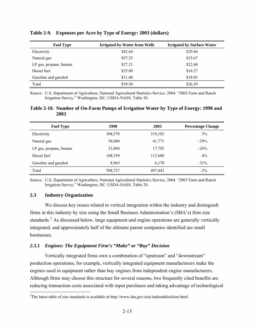
Table 2-9. Expenses per Acre by Type of Energy: 2003 (dollars)

Fuel Type Irrigated by Water from Wells Irrigated by Surface Water Electricity $42.64 $29.84 Natural gas $57.25 $33.67 LP gas, propane, butane $27.21 $22.68 Diesel fuel $25.09 $16.27 Gasoline and gasohol $11.60 $18.05 Total $39.50 $26.39

Source: U.S. Department of Agriculture, National Agricultural Statistics Service. 2004. “2003 Farm and Ranch Irrigation Survey.” Washington, DC: USDA-NASS. Table 20.

Table 2-10. Number of On-Farm Pumps of Irrigation Water by Type of Energy: 1998 and 2003

Fuel Type 1998 2003 Percentage Change

Electricity 308,579 319,102 3%

Natural gas 58,880 41,771 –29%

LP gas, propane, butane 23,964 17,792 –26%

Diesel fuel 108,339 112,600 4%

Gasoline and gasohol 8,965 6,178 –31%

Total 508,727 497,443 –2%

Source: U.S. Department of Agriculture, National Agricultural Statistics Service. 2004. “2003 Farm and Ranch Irrigation Survey.” Washington, DC: USDA-NASS. Table 20.

2.3 Industry Organization

We discuss key issues related to vertical integration within the industry and distinguish firms in this industry by size using the Small Business Administration’s (SBA’s) firm size standards.2 As discussed below, large equipment and engine operations are generally vertically integrated, and approximately half of the ultimate parent companies identified are small businesses.

2.3.1 Engines: The Equipment Firm’s “Make” or “Buy” Decision

Vertically integrated firms own a combination of “upstream” and “downstream” production operations; for example, vertically integrated equipment manufacturers make the engines used in equipment rather than buy engines from independent engine manufacturers. Although firms may choose this structure for several reasons, two frequently cited benefits are reducing transaction costs associated with input purchases and taking advantage of technological 2The latest table of size standards is available at http://www.sba.gov/size/indextableofsize.html.

2-13

economies that arise through integrated production structures (Viscusi, Vernon, and Harrington, 1992). A review of the Power Systems Research (PSR) data for 2002 shows that vertical operations are more likely to occur within large public and private firms. In addition, 80% of small specialty engine manufacturers produce and sell engines to other independent equipment companies.

2.3.2 Distribution of Small and Large Firms

EPA identified key firms using PSR data from 2002 (PSR, 2004). Although the information in PSR’s database was separated by fuel, size range, and application type, it includes both mobile and stationary engines (Parise, 2006). Using these data to identify company names has some limitations because the data set contains companies that produce mobile only, stationary only, or mobile and stationary engines. We acknowledge these limitations in identifying potentially affected stationary SI companies.

Small entities include small businesses, small organizations, and small governmental jurisdictions. A small entity is defined as follows:

a small business whose parent company has fewer than 1,000 employees (for NAICS 335312 [Motor and Generator Manufacturing] and NAICS 333618 [Other Engine Equipment Manufacturing])

a small business whose parent company has fewer than 500 employees (for NAICS 333911 [Pump and Pumping Equipment Manufacturing], NAICS 333912 [Air and Gas Compressor Manufacturing], NAICS 333111 [Farm Machinery and Equipment Manufacturing], and NAICS 333992 [Welding and Soldering Equipment Manufacturing])

a small governmental jurisdiction that is a government of a city, county, town, school district, or special district with a population of fewer than 50,000

a small organization that is any not-for-profit enterprise, which is independently owned and operated and is not dominant in its field

We identified 21 engine companies and 72 equipment companies and obtained sales and employment data for 81 of these companies (87%). Using SBA size standards and ultimate parent employment data, our analysis indicates that 34 ultimate parent companies are small businesses (37%). PSR data suggest that small businesses manufacture a small share of total engines (6% in 2002) (see Table 2-11). However, approximately one-quarter of affected equipment is manufactured by small businesses.

2-14

Table 2-11. Distribution of Engine and Equipment Production by Business Size: 2002 and Earlier Years

2002 2001 2000

Engines

Small 875 988 1,630

Large 13,327 14,669 13,292

Total 14,201 15,657 14,455

Equipment

Small 3,583 2,947 1,290

Large 10,618 12,711 13,165

Total 14,201 15,657 14,455

Note: PSR production levels have been scaled using stationary fractions of total engine sales reported by Parise (2006).

Source: Power Systems Registry (PSR). 2004. OELink™. (http://www.powersys.com/OELink.htm>.

Using SBA firm size standards, 16 engine companies are large (76%) with annual sales typically exceeding $1 billion. The remaining five engine companies are small (24%) with annual sales typically falling below $500 million (see Figures 2-2 and 2-3)

Approximately half of the equipment companies with sales data (31 total) are large companies, while the remaining 29 equipment companies are small. As shown in Figure 2-4, annual employment for these equipment companies is concentrated above 1,000 employees (40%) and below 100 employees (25%). As shown in Figure 2-5, annual sales for these equipment companies is relatively evenly distributed. Twenty-five percent of these companies have annual sales above $1 billion, 15% have annual sales between $100 and $500 million, and 23% have annual sales between $10 and $50 million.

2.4 Historical Market Data

Generator sets and welding applications are the only sectors showing growth from 1998 to 2002 (see Table 2-12). The strongest growth occurred in the 175 to 300 hp category. In contrast, pumps, compressors, and irrigation systems all experienced declines in sales during this 5-year period.

2-15

0%

10%

20%

30%

40%

50%

60%

70%

80%

<100 100–250 250–500 500–750 750–1,000 >1,000

Parent Company Employment Range

Shar

e of

Firm

s (%

)

Figure 2-2. Engine Companies’ Employment Distribution, 2005 (N = 21) Sources: Hoover’s Online. <http://www.hoovers.com>. W&D Partners Worldscape through LexisNexis. Dun & Bradstreet Small Business Solutions <http://smallbusiness.dnb.com/default.asp

?bhcd2=1107465546>. Graham & Whiteside Major Companies Database through LexisNexis.

0%

10%

20%

30%

40%

50%

60%

70%

80%

90%

<$5 $5–$10 $10–$50 $50–$100 $100–$500 $500–$1,000 >$1,000

Parent Company Revenue Range ($millions)

Shar

e of

Firm

s (%

)

Figure 2-3. Engine Companies’ Sales Distribution (N = 21) Sources: Hoover’s Online. <http://www.hoovers.com>. W&D Partners Worldscape through LexisNexis. Dun & Bradstreet Small Business Solutions <http://smallbusiness.dnb.com/default.asp


2-16

0%

5%

10%

15%

20%

25%

30%

35%40%

45%

<100 100–250 250–500 500–750 750–1,000 >1,000

Parent Company Employment Range

Shar

e of

Firm

s (%

)

Figure 2-4. Equipment Companies’ Employment Distribution, 2005 (N = 60) Sources: Hoover’s Online. <http://www.hoovers.com>. W&D Partners Worldscape through LexisNexis. Dun & Bradstreet Small Business Solutions <http://smallbusiness.dnb.com/default.asp


0%

5%

10%

15%

20%

25%

30%

<$5 $5–$10 $10–$50 $50–$100 $100–$500 $500–$1,000 >$1,000

Parent Company Revenue Range ($millions)

Shar

e of

Firm

s (%

)

Figure 2-5. Equipment Companies’ Sales Distribution (N = 60) Sources: Hoover’s Online. <http://www.hoovers.com>. W&D Partners Worldscape through LexisNexis. Dun & Bradstreet Small Business Solutions <http://smallbusiness.dnb.com/default.asp


2-17

Table 2-12. Estimated Historical Unit Sales Data by Market: 1998–2002

2002 2001 2000 1999 1998

Stationary Generator Sets and Welders

25–50 1,484 1,909 1,691 1,765 891

50–100 2,575 2,054 2,045 2,365 1,807

100–175 4,252 6,659 4,901 6,510 3,911

175–300 1,908 995 840 983 886

300–600 1,011 952 963 1,200 1,034

600–750 67 88 83 70 64

>750 1,107 1,043 1,041 976 791

Total 12,404 13,700 11,564 13,868 9,384

Stationary Pumps and Compressors

25–50 32 35 61 74 75

50–100 151 151 126 129 269

100–175 199 223 710 754 773

175–300 92 107 234 306 349

300–600 192 238 375 515 559

600–750 52 60 85 111 106

>750 505 567 844 1,026 1,102

Total 1,222 1,381 2,436 2,915 3,234

Stationary Irrigation Systems

50–100 0 0 72.9 97.8 120.3

100–175 415.2 469.6 360.8 371.2 495.2

175–300 143.65 88.4 0 0 0

Total 559 558 434 469 616

Note: Total PSR population sales were multiplied by the stationary fraction of total engine sales reported by Parise (2006).

2-18

2.4.1 Price Trends

Prices for equipment and engines have increased moderately over the last decade with the rate of increases comparable to other manufacturing industries (see Figure 2-6). Since 2003, prices have risen more quickly relative to previous years as costs of key material inputs have increased. For example, Lincoln Electric cited the rising cost of steel as a key factor influencing production costs (Lincoln Electric, 2006).

98

103

108

113

118

123

128

133

138

1995 1996 1997 1998 1999 2000 2001 2002 2003 2004 2005

Adj

uste

d Pr

oduc

er P

rice

Inde

x (B

ase

Perio

d: D

ec 9

5 =

100)

Motor and Generator Welding and Soldering EquipmentPump and Pumping Equipment Air and Gas Compressor Farm Machinery and Equipment Gasoline Nonautomotive Engines Total U.S. Manufacturing

Figure 2-6. Price Trends for Equipment and Engines Note: Price data for 2005 are preliminary estimates made by BLS that are subject to future revisions.

Source: U.S. Bureau of Labor Statistics. 2006. Series PCU335312335312, PCU333992333992, PCU333911333911, PCU333912333912, PCU333111333111, PCU3336183336181, PCUOMFG—OMFG.

2.5 Projections

Using 10-year growth data for engines (Parise, 2006), the Agency estimated that stationary SI engine markets will continue to grow at historical rates (see Table 2-13). The total affected population is estimated to grow from 26,684 to 28,898 engines between 2006 and 2015.

2-19

Table 2-13. Projected Unit Sales Data by Horsepower Range: Selected Years

HP Range 2006 2010 2015

25–50 3,027 3,509 3,991

50–100 2,531 2,477 2,423

100–175 4,895 4,935 4,974

175–300 2,389 2,552 2,715

300–600 1,658 1,942 2,227

600–750 56 15 0

>750 12,129 12,348 12,567

Total 26,684 27,778 28,898

a The projected number of new SI engines does not include new 2-stroke lean burn (2SLB) engines.

Source: Parise, T., Alpha-Gamma Technologies, Inc. 2006. Memorandum: “Population and Projection of Stationary Spark Ignition Engines.”

2-20

SECTION 3 COSTS, ECONOMIC IMPACT ANALYSIS, AND EMISSIONS

EPA prepares an EIA to provide decision makers with a measure of the social costs of using resources to comply with a program (EPA, 2000). The analysis generally includes the development of one or more partial equilibrium market models that estimate price and consumption changes and the associated measures of social costs (as measured by changes in consumer and producer surplus). However, data quality and uncertainties prevented a full specification and numerical partial equilibrium model for this analysis. As a result, EPA used a more qualitative approach to assess economic impacts. Besides the economic impacts, this section also provides the engineering cost estimates that are used to generate the economic impacts, and also the baseline emissions and emission reductions associated with this final rule.

3.1 Cost Estimate Background

The costs presented in this section are calculated based on the control cost methodology presented in the EPA (2002) Air Pollution Control Cost Manual prepared by the U.S. Environmental Protection Agency. This methodology sets out a procedure by which capital and annualized costs are defined and estimated, and this procedure is often used to estimate the costs of rulemakings such as this one. The capital costs presented in this section are annualized using a 7% interest rate, a rate that is consistent with the guidance provided in the Office of Management and Budget’s (OMB’s) (2003) Circular A-4. Equipment lives for the control technologies employed in this analysis can vary greatly (usually from 5 to 20 years).

The emission reductions from the NSPS and NESHAP are almost entirely—98%—from application of non-selective catalytic reduction (NSCR) on rich burn natural gas fired engines. An NSCR is estimated to reduce 90% of NOx, 90% of CO, 50% of non-methane hydrocarbons (NMHC), and 90% of HAP. The cost analysis assumes that most of the other affected SI engines could meet the emissions requirements in this NSPS without add-on control technology. Of these other affected SI engines, purchasing an engines certified by a manufacturer or, in the case of major HAP sources between 250–500 horsepower (HP), use of an oxidation catalyst is the basis for the emission reductions estimated for these sources.3

3.2 Regulatory Program Cost Estimates

The real-resource costs associated with the NSPS and NESHAP programs include the cost of installing and maintaining air pollution control equipment; the activities related to engine 3Parise, T., Alpha-Gamma Technologies, Inc. 2007. Memorandum: “Cost Impacts and Emission Reductions

Associated with Final NSPS for Stationary SI ICE and NESHAP for Stationary RICE.”

3-1

certification for manufacturers; and the cost of initial notification, record keeping, and testing for certain engine owners and operators (see Table 3-1). EPA estimates total annualized costs of all the NSPS requirements will be $18.6 million (2005 dollars) for the year 2015, and costs for all the NESHAP requirements alone to be $3.1 million (2005 dollars) for the year 2015.

Table 3-1. Average Total Cost per Engine: 2015 (2005$)

NSPS Total Annual Costs Number of Affected Engines Average Total Cost

($/Engine)

25–50 $1,763,468 3,509 $503

50–100 $2,831,776 2,477 $1,143

100–175 $5,320,088 4,935 $1,078

175–300 $2,383,658 2,552 $934

300–600 $2,385,269 1,942 $1,228

600–750 $20,539 15 $1,385

750> $3,890,281 2,627 $1,481

Total $18,595,080 18,057 $1,030

NESHAP $3,170,231 416 $7,621

Source: Parise, T., Alpha-Gamma Technologies, Inc. 2007. Memorandum: “Cost Impacts and Emission Reductions Associated with Final NSPS for Stationary SI ICE and NESHAP for Stationary RICE.” Appendix A.

To make industry-level economic impact assessments that will provide an estimate on an average impact per firm, EPA compared the engineering cost estimates in 2015 with the projected value of shipments for these industries in 2015.4 As shown in Table 3-2, the industry-level cost-to-sales ratios are at or below 0.10%. These industry-level cost-to-sales ratios can be interpreted as an average impact on potentially affected firms in these industries. Based on this estimate of cost-to-sales ratios, we can conclude that the annualized cost of this rule should be no higher than 0.10% of the sales for a firm in each of these industries. The industries listed in Table 3-2 have a ratio of parent businesses to establishments that is close to 1:1,5 thus, there are few parent businesses in these industries that own more than one establishment.6 Given the small business size standards shown later in Section 5, we can show that a majority of the businesses in these industries are small. For example, NAICS 335312 contains 453 businesses that own 594 establishments. All but four of these establishments have 1,000 employees or less, and 1,000

4The projected value of shipments was estimated using the AEO 2007’s (EIA, 2007) metal-based durables sector

shipment growth rates for NAICS 333 (Machinery) and NAICS 335 (Electrical Equipment). 5Based on data from U.S. Census Bureau, 2002 Economic Census, Manufacturing-Industry Series. Tables for

Industry Statistics by Employment Size: 2002. These tables for each industry are found at http://www.census.gov/econ/census02/guide/INDRPT31.HTM.

6An establishment is a place for a business to operate; a parent business can own more than one establishment.

3-2

http://www.census.gov/econ/census02/guide/INDRPT31.HTM

employees the small business size standard established by the Small Business Administration (SBA) as mentioned later in Section 5. Hence, we can presume that most of the businesses in this industry are small businesses. Thus, the cost to sales ratios in Table 3-2 are representative of impacts to small businesses affected by this final rule.

Table 3-2. Comparison of Regulatory Program Costs and Value of Shipments: 2015

Industry (NAICS)

Total Annual Costs ($ million)a

Value of Shipments: 2005

($billion) a

Estimated Value of Shipments: 2015

($billion) a Cost-to-Sales Ratio

333912 $5.8 $6.9 $8.4 0.07%

335312 $14.5 $11.5 $14.5 0.10%

333911 $0.8 $9.1 $11.1 0.01%

333992 $0.6 $3.8 $4.6 0.01%

a All values are expressed in 2005 dollars.

Sources: Parise, T., Alpha-Gamma Technologies, Inc. 2007. Memorandum: “Cost Impacts and Emission Reductions Associated with Final NSPS for Stationary SI ICE and NESHAP for Stationary RICE.” Appendix A.

U.S. Bureau of the Census. 2006. “Annual Survey of Manufacturers.” Statistics for Industry Groups and Industries: 2005. M05(AS)-1. Washington, DC: U.S. Bureau of the Census. Table 2.

U.S. Energy Information Administration (EIA). 2007. Annual Energy Outlook 2007. Supplemental Table 32. Washington, DC: U.S. Energy Information Administration.

3.3 Economic Framework

Given data limitations and uncertainties regarding supply and demand equations in affected markets, EPA used a stylized model to support conclusions regarding the economic impacts of the final rule. This model examines changes in long-run equilibrium in response to increases in per-unit production costs. The market supply function is assumed to be horizontal in this model because marginal costs are constant as output changes (EPA, 1999). Market demand is represented by the standard downward-sloping curve. The market is assumed here to be perfectly competitive; equilibrium is determined by the intersection of the supply and demand curves.

A change in unit-production costs shifts the market supply curve for engines (see Figure 3-1). As shown in the figure, the cost increase causes the market price to increase by the full amount of the per-unit control cost (i.e., from P0 to P1). This scenario is typically referred to as “full-cost pass-through” because the costs are passed on to downstream buyers in the form of higher prices. A rise in the equilibrium market price will also lead to a reduction in consumption.

3-3

Unit Cost Increase}PriceIncrease

}

Q1 Q0

S1: With Regulation

S0: Without Regulation

P1

P0

D

c b

a

$

Output

d

Figure 3-1. Long Run: Full-Cost Pass-Through

3.4 Conclusions for Economic Impacts

Using average total cost data from the engineering cost memos prepared for this final rule, the NSPS standard could result in an average price increase for engines of $1,030 (see Table 3-1). The price increases would likely vary by engine horsepower and range from $503 per engine to $1,481 per engine. The NESHAP requires additional controls for a very small subset of the engine population (250 to 500 hp 4SLB SI engines located at major sources). Price increases for these engines could be as high as $7,621 per engine. Although baseline price data for these engines affected by the NESHAP are not available, EPA’s analysis for the nonroad rule (EPA, 2004; Table 10.3-6) provides a proxy for engine prices. Using these baseline price data and average total cost data suggests potential percentage changes in engine prices range from 5% to 33%. Price increases for engines less than 175 hp would experience the highest increases (17% to 33%), while engines over 175 hp would experience increases ranging from 5% to 7%.

EPA considered potential consumption changes using the price elasticity of demand, which refers to the percentage change in quantity demanded resulting from a percentage change in the price of the good. Economic theory and other EPA economic models of engine markets suggest these elasticities are likely to be inelastic and very small as shown in EPA’s economic analysis of the nonroad rule (EPA, 2004). As a result, EPA believes changes in engine consumption will be much smaller than the percentage increases in price discussed above. For

3-4

example, if we consider the range of percentage change in prices above and assume a constant price elasticity of demand of –0.10, engine consumption could potentially fall between 0.5% to 3.3%.

EPA’s Guidelines for Preparing Economic Analyses (EPA, 2000; p. 125) notes there is little practical difference between social cost estimates derived from a perfect competition partial equilibrium model and engineering compliance cost estimates when consumption changes are small. Given the consumption change analysis above, EPA believes the national annualized compliance cost estimates provide a reasonable approximation of the social cost of this regulatory program. The engineering analysis estimated annualized costs of $21.7 million in 2015 for the NSPS and NESHAP combined.

3.5 Baseline Emissions and Emission Reductions

Table 3-3 presents the baseline emissions estimated for this final rule in 2015, which is the analysis year for this RIA. Table 3-4 presents the emission reductions estimated for this final rule in 2015.

Table 3-3. Baseline Emissions in 2015 by Engine Size Category

Baseline Emissions by Pollutant (tons)

Engine Size (hp)

Engine Population by Size* NOx

CO

NMHC HAP

25-50 3,510 5,125 4,519 84 31 50-100 2,478 7,093 6,272 117 44 100-175 4,935 18,702 16,540 871 327 175-300 2,551 11,871 9,645 896 336 300-500 1,296 11,060 6,607 665 249 500-600 647 5,337 3,704 499 187 600-750

14 146 104 14 5

750-1200 1,493 20,908 16,996 2,151 807 1200-2000 807 11,629 12,206 2,329 873 >2000 326 2,088 4,283 1,088 408

TOTAL:

18,057 93,958 80,876 8,714 3,268 hp = horsepower; NMHC = non-methane hydrocarbons

3-5

* These engine counts are the sum of the new engines expected to be affected by the final NSPS for specific engine size categories in 2015. The vast majority of these engines are prime engines that are natural gas-fired. More detailed information on these engines can be found in the cost impacts memorandum prepared for this final rule.7

Table 3-4. Emission Reductions in 2015 by Engine Size Category

Emission Reductions by Pollutant (tons)

Engine Size (hp)

Engine Population by Size* NOx

CO

NMHC HAP

25-50 3,510 4,595 2,851 40 15 50-100 2,478 6,273 4,764 79 30

100-175 4,935

16,737 11,892 442 166 175-300 2,551 10,200 5,658 322 121 300-500 1,296 9,765 3,891 286 107 500-600 647 4,414 1,769 110 41 600-750

14 120 50 3 1

750-1200 1,493 17,130 9,085 509 191 1200-2000 807 8,012 4,735 356 133 >2000 326 116 265 0 0

TOTAL:

18,057 77,362 44,959 2,146 805 hp = horsepower; NMHC = non-methane hydrocarbons

* These engine counts are the sum of the new engines expected to be affected by the final NSPS for specific engine size categories in 2015. The vast majority of these engines are prime engines that are natural gas-fired. More detailed information on these engines can be found in the cost impacts memorandum prepared for this final rule.8

The emission reductions of NOx associated with this final rule are estimated at 77,362 tons in 2015. This represents an 82 percent reduction from the baseline NOx emissions of 93,958 tons in 2015. These tables also show reductions of 56% of CO emissions, 25% of NMHC emissions, and 25% of HAP emissions. 9

7 Parise, T., Alpha-Gamma Technologies, Inc. 2007. Memorandum: “Cost Impacts and Emission Reductions

Associated with Final NSPS for Stationary SI ICE and NESHAP for Stationary RICE.” 8 Parise, T., Alpha-Gamma Technologies, Inc. 2007. Memorandum: “Cost Impacts and Emission Reductions

Associated with Final NSPS for Stationary SI ICE and NESHAP for Stationary RICE.” 9 Parise, T., Alpha-Gamma Technologies, Inc. 2007. Memorandum: “Cost Impacts and Emission Reductions

Associated with Final NSPS for Stationary SI ICE and NESHAP for Stationary RICE.” Appendix B and C.

3-6

SECTION 4 ENERGY IMPACTS

Executive Order 13211 (66 FR 28355, May 22, 2001) provides that agencies will prepare and submit to the Administrator of the Office of Information and Regulatory Affairs, Office of Management and Budget, a Statement of Energy Effects for certain actions identified as “significant energy actions.” Section 4(b) of Executive Order 13211 defines “significant energy actions” as

any action by an agency (normally published in the Federal Register) that promulgates or is expected to lead to the promulgation of a final rule or regulation, including notices of inquiry, advance notices of proposed rulemaking, and notices of proposed rulemaking: (1) (i) that is a significant regulatory action under Executive Order 12866 or any successor order, and (ii) is likely to have a significant adverse effect on the supply, distribution, or use of energy; or (2) that is designated by the Administrator of the Office of Information and Regulatory Affairs as a significant energy action.

This rule is not a significant energy action as designated by the Administrator of the Office of Information and Regulatory Affairs because it is not likely to have a significant adverse impact on the supply, distribution, or use of energy. EPA has prepared an analysis of energy impacts that explains this conclusion as follows below.

To enhance understanding regarding the regulation’s influence on energy consumption, we examined publicly available data describing energy consumption for industries that will be affected by this rule. The Annual Energy Outlook 2007 (EIA, 2007) provides energy consumption rates (Btu per dollar of shipments) by fuel type for a broad set of industries (NAICS 333 [Machinery] and NAICS 335 [Electrical Equipment]) that include those affected by this rule. We applied these rates to the projected value of shipments for NAICS codes 333912, 335312, 333911, and 333992 to obtain estimates of energy consumption for the affected industries.10 As shown in Table 4-1, the four sectors are expected to consume 11.1 trillion Btus of liquid fuels and other petroleum, 13.8 trillion Btus of natural gas, and 15.1 trillion Btus of electricity. A comparison of these data to U.S. delivered energy consumption illustrates that these industries account for less than 0.10% of the U.S. total for each fuel type. As a result, any energy consumption changes attributable to the regulatory program should not significantly influence the supply, distribution, or use of energy. 10Details on the industry shipment projection calculations are provided in Section 3. We have adjusted these

estimates to reflect 2000 dollars using the gross domestic product deflator.

4-1

Table 4-1. Affected Industry Share by Fuel Type: 2015

Energy Consumption (trillion Btu)

NAICS

Estimated Value of Shipment: 2015 (billion 2000$)

Liquid Fuels and Other Petroleum

Subtotal Natural Gas Electricity

333912 $9.5 0.043 2.25 2.75

335312 $16.3 10.91 7.39 7.23

333911 $12.4 0.056 2.96 3.62

333992 $5.2 0.023 1.24 1.51

Affected Industry Total 11.06 13.83 15.11

US Total Delivered Energy Consumption: 43,290 18,763 14,506

Affected Share: 0.03% 0.07% 0.10%

Source: U.S. Department of Energy. 2007. Annual Energy Outlook. Supplemental Tables to Energy Annual Outlook. Tables 2, 32.

4-2

SECTION 5 SMALL BUSINESS IMPACT ANALYSIS

The Regulatory Flexibility Act (RFA) generally requires an agency to prepare a regulatory flexibility analysis of any rule subject to notice and comment rulemaking requirements under the Administrative Procedure Act or any other statute unless the agency certifies that the rule will not have a significant economic impact on a substantial number of small entities (SISNOSE). Small entities include small businesses, small organizations, and small governmental jurisdictions.

5.1 Description of Small Entities Affected

For the purposes of assessing the impacts of this rule on small entities, small entity is defined as (1) a small business based on the following SBA size standards, which are based on employee size: NAICS 333911 B Pump and Pumping Equipment Manufacturing—500 employees or fewer; NAICS 333912 B Pump and Compressor Manufacturing—500 employees or fewer; NAICS 33399P—All Other Miscellaneous General Purpose, Machinery—500 employees or fewer; NAICS 335312 B Motor and Generator Manufacturing—1,000 employees or fewer; and NAICS 333618—Other Engine Equipment Manufacturing—1,000 employees or fewer; (2) a small governmental jurisdiction that is a government of a city, county, town, school district, or special district with a population of fewer than 50,000; and (3) a small organization that is any not-for-profit enterprise that is independently owned and operated and is not dominant in its field. For more information, refer to http://www.sba.gov/size/sizetable2002.html. The small entity impacts of this rule are estimated in terms of comparing the compliance costs to revenues at affected firms.

5.2 Small Business Screening Analysis

In the next step of the analysis, we assessed how the regulatory program may influence the profitability of ultimate parent companies by comparing pollution control costs to total sales. To do this, we divided an ultimate parent company’s total annual compliance cost by its reported revenue:

j

n

iTR

TACC

CSR

∑= (5.1)

5-1

where

CSR = cost-to-sales ratio,

TACC = total annualized compliance costs,

i = index of the number of affected plants owned by company j,

n = number of affected plants, and

TRj = total revenue from all operations of ultimate parent company j.

This method assumes the affected company cannot shift pollution control costs to consumers (in the form of higher market prices). Instead, the company experiences a one-for-one reduction in profits.

To identify sales and employment characteristics of affected parent companies, we used a company database developed for the small business analysis of the Bond Amendments Rule. Since the rule does not affect all companies included in the database, the analysis only includes companies that produced the following types of equipment segments:

pumps and compressors (Pump and Pumping Equipment Manufacturing [NAICS 333911] or Air and Gas Compressor Manufacturing [NAICS 333912]) and

welders and generators (Motor and Generator Manufacturing [NAICS 335312] or Welding and Soldering Equipment Manufacturing [NAICS 333992]).

The statistics included in the database come from PSR (Power Systems Research) and other publicly available resources such as the following:

LexisNexis Academic Universe: A single database for company profiles, executives, revenue, and competitors; detailed financial information; full-text articles; investment reports; and industry overviews. Company information can be searched by name, address, Standard Industrial Classification (SIC), or ticker symbol. www.lexisnexis.com/academic/universe/academic/.

Hoover’s Online: This electronic database is an excellent source of information on U.S. public and private companies. Users can search for companies by name, ticker symbol, or keyword. It provides corporate ownership, sales, net income, and employment. Links are also provided to the company’s Web site and those of top competitors (if available), Securities and Exchange Commission (SEC) filings in EDGAR Online, investor research reports, and news and commentary. http://www.hoovers.com/.

Dun & Bradstreet’s Million Dollar Directory: The D&B Million Dollar Directory provides information on over 1,260,000 leading U.S. public and private businesses. Company information includes industry information with up to 24 individual eight-digit SIC codes, size criteria (employees and annual sales), type of ownership, and

5-2

principal executives and biographies. http://www.dnb.com/dbproducts/description/ 0,2867,2-223-1012-0-223-142-177-1,00.html.

Among the companies that manufacture engines, we identified 5 small companies and 16 large companies with sales data. All of them are included in the Other Engine Equipment Manufacturing (NAICS 333618) industry.

The results of the screening analysis, presented in Table 5-1, show that one firm has a CSR greater than 3%. The remaining 20 small firms have estimated CSRs below 1%. The average (median) CSR for small firms is 1.02% (0.02%), and the average and median CSR for all large firms with data is less than 0.01% (0.001%).

Table 5-1. Summary Statistics for SBREFA Screening Analysis

Small Large

Number Share (%) Number Share (%)

Companies with Parent Sales Data 5 100% 16 100%

Compliance costs are <1% of sales 4 80% 16 100%

Compliance costs are ≥1% to 3% of sales 0 0% 0 0%

Compliance costs are ≥3% of sales 1 20% 0 0%

Cost-to-Sales Ratios (%)

Average 1.02% 0.01%

Median 0.02% <0.01%

Maximum 4.94% 0.08%

Minimum 0.00% 0.00%

5.3 Assessment Results and Conclusions

After considering the economic impacts of this rule on small entities, the Agency certifies that this rule will not have a significant economic impact on a substantial number of small entities. This rule is expected to affect 21 ultimate parent businesses that are manufacturers of affected small SI engines. Five of the parent businesses are small according to the SBA small business size standard. One of these five businesses would have an annualized cost of more than 1% of sales associated with meeting the requirements; the estimated cost is approximately 5% for this small firm. In addition, for the industries in which small businesses are found that may be affected by this final rule, either by purchasing a compliant SI engine or by performing the required testing, the estimated cost of this rule is 0.10% of sales or less as shown in Chapter 3 of this RIA. Also, no other adverse impacts are expected to these affected small businesses.

5-3

Although this rule would not have a significant economic impact on a substantial number of small entities, the Agency nonetheless tried to reduce the impact of this rule on small entities. When developing the revised standards, the Agency took special steps to ensure that the burdens imposed on small entities were minimal. The Agency conducted several meetings with industry trade associations to discuss regulatory options and the corresponding burden on industry, such as record keeping and reporting.

5-4

SECTION 6 HUMAN HEALTH BENEFITS OF EMISSIONS REDUCTIONS

6.1 Calculation of Human Health Benefits

For the purposes of estimating the human health benefits of reducing emissions from SI engines through this rulemaking, EPA is using the benefits transfer approach and methodology found in the Technical Support Document (TSD) accompanying the 2007 RIA supporting the proposed changes to the Ozone National Ambient Air Quality Standards.11

,12 In that RIA, EPA applied a

benefits transfer approach to estimate the PM2.5

2.5

2.5 x

2.5

benefits resulting from reductions in emissions of NOx; EPA is adapting that method to estimate the PM -related health benefits for the projected emission reductions associated with this rulemaking. EPA did not perform an air quality modeling assessment of the emission reductions resulting from installing controls on these engines because of resource constraints and the limited value of such an analysis for the purposes of developing the regulatory approach for this final rule. This lack of air quality modeling limited EPA’s ability to perform a comprehensive benefits analysis for this rulemaking since our benefits model requires either air quality modeling or monitoring data. The benefits transfer approach described in the TSD accompanying the Ozone RIA consists of benefit per ton estimates that relate a 1-ton reduction in a given PM precursor, such as NO emitted by stationary sources, to an estimate of the total monetized human health benefits of reduced exposure to PM . Readers interested in the methodology followed to generate these estimates may consult the TSD supporting the Ozone RIA (EPA, 2007).

To develop the estimate of the benefits of the emission reductions from the SI rulemaking, we multiplied the estimated NOx emission reduction against the stationary source NOx benefit-per-ton estimate found in the TSD described above. We summarize these results in Table 6-1. It is important to note that the dollar benefit-per-ton estimates used here reflect specific geographic patterns of emissions reductions and specific air quality and benefits modeling assumptions. Use of these dollar-per-ton values to estimate benefits associated with different emission control programs (e.g., for reducing emissions from large stationary sources like EGUs) may lead to higher or lower benefit estimates than if benefits were calculated based on direct air quality modeling. Great care should be taken in applying these estimates to emission reductions occurring in any specific location, because these are all based on national or broad

11 U.S. Environmental Protection Agency (EPA). 2007. Regulatory Impact Analysis of the Proposed Changes to the

Ozone National Ambient Air Quality Standards. 12 U.S. Environmental Protection Agency (EPA). 2006. Technical Support Document: Calculating Benefit per-Ton

Estimates. EPA-HQ-OAR-2006-0834.

6-1

regional emission reduction programs and therefore represent average benefits per ton over the entire United States. The benefits per ton for emission reductions in specific locations may be very different from the national average. Finally, in this table we provide an estimate of total

Table 6-1. Estimate of Monetized Benefits by 2015 ($2005)a

$ Benefits/Ton Amount of NOx Emissions

Reduced (tons) Monetized Benefits (millions of

2005$)b

$2,800 to $6,100 77,362 $220 to $470

a The results in the table are presented assuming a discount rate of 3%. b Estimate rounded to two significant figures.

benefits using two different benefit-per-ton estimates. Each benefit-per-ton estimate was derived using a different PM2.5 mortality health impact function; the first estimate uses the Pope et al. (2002) function, while the second uses the Laden et al. (2006) function. We discuss this difference in further detail below.

6.2 Characterization of Uncertainty in the Benefits Estimates

In any complex analysis, there are likely to be many sources of uncertainty. Many inputs are used to derive the final estimate of economic benefits, including emission inventories, air quality models (with their associated parameters and inputs), epidemiological estimates of concentration-response (C-R) functions, estimates of values, population estimates, income estimates, and estimates of the future state of the world (i.e., regulations, technology, and human behavior). For some parameters or inputs it may be possible to provide a statistical representation of the underlying uncertainty distribution. For other parameters or inputs, the necessary information is not available.

The annual benefit estimates presented in this analysis are also inherently variable due to the processes that govern pollutant emissions and ambient air quality in a given year. Factors such as hours of equipment use and weather are constantly variable, regardless of our ability to accurately measure them. Thus, the estimates of annual benefits should be viewed as representative of the magnitude of benefits expected, rather than the actual benefits that would occur every year.

Above we present a primary estimate of the total benefits, based on our interpretation of the best available scientific literature and methods and supported by the Science Advisory Board–Health Effects Subcommittee (SAB-HES) and the National Academy of Science (NAS) (NRC, 2002). The benefits estimates are subject to a number of assumptions and uncertainties.

6-2

For example, key assumptions underlying the primary estimate for the premature mortality, which typically accounts for at least 90% of the total benefits we were able to quantify include the following:

1. Inhalation of fine particles is causally associated with premature death at concentrations near those experienced by most Americans on a daily basis. Although biological mechanisms for this effect have not yet been definitively established, the weight of the available epidemiological evidence supports an assumption of causality.

2. All fine particles, regardless of their chemical composition, are equally potent in causing premature mortality. This is an important assumption, because PM produced via transported precursors emitted from EGUs may differ significantly from direct PM released from diesel engines and other industrial sources, but no clear scientific grounds exist for supporting differential effects estimates by particle type.

3. The impact function for fine particles is approximately linear within the range of ambient concentrations under consideration. Thus, the estimates include health benefits from reducing fine particles in areas with varied concentrations of PM, including both regions that are in attainment with the fine particle standard and those that do not meet the standard.

4. The forecasts for future emissions and associated air quality modeling are valid. Although recognizing the difficulties, assumptions, and inherent uncertainties in the overall enterprise, these analyses are based on peer-reviewed scientific literature and up-to-date assessment tools, and we believe the results are highly useful in assessing this rule.

The NAS (2002) report on estimating public health benefits of air pollution regulations recommended that EPA begin to move the assessment of uncertainties from its ancillary analyses into its primary analyses by conducting probabilistic, multiple-source uncertainty analyses. As part of a collaboration between EPA’s Office of Air and Radiation (OAR) and the OMB on the Nonroad Diesel Rule, we conducted a pilot expert elicitation intended to more fully characterize uncertainty in the estimate of mortality resulting from exposure to PM. In 2006, EPA completed a full-scale expert elicitation that incorporated peer-review comments on the pilot application and that provides a more robust characterization of the uncertainty in the premature mortality function. This expert elicitation was designed to evaluate uncertainty in the underlying causal relationship, the form of the mortality impact function (e.g., threshold versus linear models), and the fit of a specific model to the data (e.g., confidence bounds for specific percentiles of the mortality effect estimates). Additional issues, such as the ability of long-term cohort studies to capture premature mortality resulting from short-term peak PM exposures, were also addressed in the expert elicitation. The results of this expert elicitation can be found in the Particulate Matter NAAQS Regulatory Impact Analysis (PM NAAQS RIA) (October 2006). When comparing the estimates of premature mortality using both the data-derived (i.e., Pope et al.,

6-3

2002) and expert elicitation project (IEc, 2006)-derived C-R functions, it is clear that the data-derived mortality estimate falls toward the lower end of the expert range. As discussed further in this document, EPA is updating its benefit-per-ton estimates to incorporate alternate data-derived and expert-derived estimates of premature mortalities avoided.

This RIA does not include the type of detailed uncertainty assessment found in the PM NAAQS RIA because we lack the necessary air quality input and monitoring data to run the benefits model. Moreover, it was not possible to develop benefit-per-ton metrics and associated estimates of uncertainty using the benefits estimates from the PM RIA because of the significant differences between the sources affected in that rule and those regulated here. However, the results of the Monte Carlo analyses of the health and welfare benefits presented in Chapter 5 of that RIA can provide some evidence of the uncertainty surrounding the benefits results presented in this analysis. The sections below detail how EPA performs such uncertainty analyses and thus provide useful insights into the uncertainties associated with the benefit estimates found in this RIA.

In our recent assessment of the PM NAAQS RIA, we describe our progress toward improving our approach of characterizing the uncertainties in our economic benefits estimates, with particular emphasis on the C-R function relating premature mortality to exposures to ambient PM2.5. We presented two approaches to generating probabilistic distributions designed to illustrate the potential influence of some aspects of the uncertainty in the C-R function in a PM benefits analysis. The first approach generated a probabilistic estimate of statistical uncertainty based on standard errors reported in the underlying studies used in the benefit modeling framework. The second approach used the results from the final expert elicitation designed to characterize certain aspects of uncertainty in the ambient PM2.5/mortality relationship.

In addition to the two approaches to characterize uncertainty for PM mortality, we incorporated information on uncertainties of other endpoints in the benefits model. We did not attempt to assign probabilities to all of the uncertain parameters in the model because of a lack of resources and reliable methods. We simply generated estimates of the distributions of dollar benefits for PM health effects and for total dollar benefits. For nonmortality endpoints, we provide a likelihood distribution for the total benefits estimate, based solely on the statistical uncertainty surrounding the estimated C-R functions and the assumed distributions around the unit values.

6-4

Our estimate of the likelihood distribution for total benefits should be viewed as incomplete because of the wide range of sources of uncertainty that we have not incorporated. The 5th and 95th percentile points of our estimate are based on statistical error, and cross-study variability provides some insight into how uncertain our estimate is with regard to those sources of uncertainty. However, it does not capture other sources of uncertainty regarding other inputs to the model, including emissions, air quality, baseline population incidence, projected exposures, or the model itself, including aspects of health science not captured in the studies, such as the likelihood that PM is causally related to premature mortality and other serious health effects. Thus, a likelihood description based on the standard error would provide a misleading picture about the overall uncertainty in the estimates.

Both the uncertainty about the incidence changes13 and uncertainty about unit dollar values can be characterized by distributions. Each “likelihood distribution” characterizes our beliefs about what the true value of an unknown variable (e.g., the true change in incidence of a given health effect in relation to PM exposure) is likely to be, based on the available information from relevant studies.14 Unlike a sampling distribution (which describes the possible values that an estimator of an unknown variable might take on), this likelihood distribution describes our beliefs about what values the unknown variable itself might be. Such likelihood distributions can be constructed for each underlying unknown variable (such as a particular pollutant coefficient for a particular location) or for a function of several underlying unknown variables (such as the total dollar benefit of a regulation). In either case, a likelihood distribution is a characterization of our beliefs about what the unknown variable (or the function of unknown variables) is likely to be, based on all the available relevant information. A likelihood description based on such distributions is typically expressed as the interval from the 5th percentile point of the likelihood distribution to the 95th percentile point. If all uncertainty had been included, this range would be the “credible range” within which we believe the true value is likely to lie with 90% probability.

6.3 Monte Carlo–Based Uncertainty Analysis

The uncertainty about the total dollar benefit associated with any single endpoint combines the uncertainties from these two sources (the C-R relationship and the valuation) and is estimated with a Monte Carlo method. In each iteration of the Monte Carlo procedure, a value is 13Because this is a national analysis in which, for each endpoint, a single C-R function is applied everywhere, there

are two sources of uncertainty about incidence: statistical uncertainty (due to sampling error) about the true value of the pollutant coefficient in the location where the C-R function was estimated and uncertainty about how well any given pollutant coefficient approximates β*.

14Although such a “likelihood distribution” is not formally a Bayesian posterior distribution, it is very similar in concept and function (see, for example, the discussion of the Bayesian approach in Kennedy [1990]), pp. 168-172).

6-5

randomly drawn from the incidence distribution, another value is randomly drawn from the unit dollar value distribution; the total dollar benefit for that iteration is the product of the two.15 When this is repeated for many (e.g., thousands of) iterations, the distribution of total dollar benefits associated with the endpoint is generated.

Using this Monte Carlo procedure, a distribution of dollar benefits can be generated for each endpoint. As the number of Monte Carlo draws gets larger and larger, the Monte Carlo–generated distribution becomes a better and better approximation of a joint likelihood distribution (for the considered parameters) making up the total monetary benefits for the endpoint. After endpoint-specific distributions are generated, the same Monte Carlo procedure can then be used to combine the dollar benefits from different (nonoverlapping) endpoints to generate a distribution of total dollar benefits.

The estimate of total benefits may be thought of as the end result of a sequential process in which, at each step, the estimate of benefits from an additional source is added. Each time an estimate of dollar benefits from a new source (e.g., a new health endpoint) is added to the previous estimate of total dollar benefits, the estimated total dollar benefits increases. However, our bounding or likelihood description of where the true total value lies also increases as we add more sources. The physical effects estimated in this analysis are assumed to occur independently. It is possible that, for any given pollution level, there is some correlation between the occurrence of physical effects, due to say avoidance behavior or common causal pathways and treatments (e.g., stroke, some kidney disease, and heart attack are related to treatable blood pressure). Estimating accurately any such correlation, however, is beyond the scope of this analysis, and instead it is simply assumed that the physical effects occur independently.

For the PM NAAQS RIA, we conducted two different Monte Carlo analyses, one based on the distribution of reductions in premature mortality characterized by the mean effect estimate and standard error from the epidemiology study of PM-associated mortality associated with the primary estimate (Pope et al., 2002), and one based on the results from the final expert elicitation project (IEc, 2006). In both analyses, the distributions of all other health endpoints are characterized by the reported mean and standard deviations from the epidemiology literature. Distributions for unit dollar values are based on reported ranges or distributions of values in the economics literature and are summarized in Table 5-11 of Chapter 5 of the PM NAAQS RIA.

15This method assumes that the incidence change and the unit dollar value for an endpoint are stochastically

independent.

6-6

6.4 Updating the Benefits Data Underlying the Benefit per Ton Estimates

As described above, the estimates in Table 6-1 are derived through a benefits transfer technique that adapts monetized benefits estimated as part of the analyses done for the proposed ozone RIA. EPA is currently generating updated benefit-per-ton estimates that better account for the spatial heterogeneity of benefits and incorporate the new expert elicitation findings discussed above. EPA believes that these updated estimates will reduce the total amount of uncertainty associated with using the benefit-per-ton approach to derive an estimate of total benefits.

6.5 Comparison of Benefits and Costs

EPA estimates the annualized benefits of this rulemaking to be $220 and $470 million (2005$) and annualized costs to be $22 million (2005$). Thus, benefits exceed costs by about $200 to $450 million in 2015. EPA believes that the benefits are likely to exceed the costs by a significant margin under this rulemaking even when taking into account uncertainties in the cost and benefit estimates.

6-7

REFERENCES

Dun & Bradstreet Small Business Solutions http://smallbusiness.dnb.com/default.asp? bhcd2=1107465546.

Graham & Whiteside Major Companies Database through LexisNexis. Available from <http://www.lexisnexis.com/>.

Hoover’s Online. 2005. Available from <http://www.hoovers.com/free>.

Industrial Economics, Incorporated (IEc). 2006. “Expanded Expert Judgment Assessment of the Relationship Between PM2.5 Exposure and Mortality.” Available from http://www.epa.gov/ttn/ecas/regdata/Uncertainty/pm_ee_report.pdf.

Interstate Oil & Gas Compact Commission. 2006. “Marginal Wells: Fuel for Economic Growth.” Table 3.A. Available from <http://www.ok.gov/marginalwells/Publications/ Surveys_and_Reports.html>.

Laden F, Schwartz J, Speizer FE, Dockery DW. 2006. Reduction in fine particulate air pollution and mortality. American Journal of Respiratory and Critical Care Medicine. 173: 667–672.

Lexis-Nexis Academic Universe. 2007. Available from www.lexisnexis.com/academic/universe/academic/.

Lincoln Electric Holdings. 2006. Form 10-K. Filed February 24, 2006.

National Research Council (NRC). 2002. Estimating the Public Health Benefits of Proposed Air Pollution Regulations. Washington, DC: The National Academies Press.

Parise, T., Alpha-Gamma Technologies, Inc. 2006. Memorandum: “Population and Projection of Stationary Spark Ignition Engines.”

Parise, T., Alpha-Gamma Technologies, Inc. 2007. Memorandum: “Cost Impacts and Emission Reductions Associated with Final NSPS for Stationary SI ICE and NESHAP for Stationary RICE.” Appendix A.

Pope, C.A., III, R.T. Burnett, M.J. Thun, E.E. Calle, D. Krewski, K. Ito, and G.D. Thurston. 2002. “Lung Cancer, Cardiopulmonary Mortality, and Long-Term Exposure to Fine Particulate Air Pollution.” Journal of the American Medical Association 287:1132-1141.

Power Systems Registry (PSR). 2004. OELink™. Available from <http://www.powersys.com/OELink.htm>.

U.S. Bureau of Economic Analysis (BEA). 2002. 1997 Benchmark Input-Output Accounts: Detailed Make Table, Use Table and Direct Requirements Table. Tables 4 and 5.

R- 1

http://smallbusiness.dnb.com/default.asp?%20%0B%20%20bhcd2=1107465546

http://smallbusiness.dnb.com/default.asp?%20%0B%20%20bhcd2=1107465546

http://www.lexisnexis.com/

http://www.epa.gov/ttn/ecas/regdata/Uncertainty/pm_ee_report.pdf



http://www.lexisnexis.com/academic/universe/academic/

U.S. Bureau of Labor Statistics (BLS). 2006. Series PCU335312335312, PCU333992333992, PCU333911333911, PCU333912333912, PCU333111333111, PCU3336183336181, PCUOMFG—OMFG.


U.S. Bureau of the Census. 2004. “Manufacturing Industry Series.” Welding and Soldering Equipment Manufacturing: 2002. EC02-31I-333992 (RV). Washington, DC: U.S. Bureau of the Census. Table 1.

U.S. Bureau of the Census. 2006. “Annual Survey of Manufacturers.” Statistics for Industry Groups and Industries: 2005. M05(AS)-1. Washington, DC: U.S. Bureau of the Census. Table 2.

U.S. Department of Agriculture (USDA), National Agricultural Statistics Service (NASS). 2004. “2003 Farm and Ranch Irrigation Survey.” Washington, DC: USDA-NASS.

U.S. Department of Energy. 2007. Annual Energy Outlook. Supplemental Tables to Energy Annual Outlook. Tables 2, 32.

U.S. Energy Information Administration (EIA). 2007. Annual Energy Outlook 2007. Supplemental Table 32. Washington, DC: U.S. Energy Information Administration.

U.S. Environmental Protection Agency (EPA). 1999. OAQPS Economic Analysis Resource Document. Research Triangle Park, NC: EPA. Available from http://www.epa.gov/ttn/ecas/econdata/6807-305.pdf.

U.S. Environmental Protection Agency (EPA). 2000. EPA Guidelines for Preparing Economic Analyses. EPA 240-R-00-003. Available from <http://yosemite.epa.gov/ee/epa.eed.nsf/webpages/guideliens.html#download>.

U.S. Environmental Protection Agency (EPA). 2004. Final Regulatory Impact Analysis: Control of Emissions from Nonroad Diesel Engines EPA420-R-04-007, May 2004. Available from <http://www.epa.gov/nonroad-diesel/2004fr/420r04007.pdf>.

U.S. Environmental Protection Agency (EPA). 2006. Technical Support Document: Calculating Benefit per-Ton Estimates. EPA-HQ-OAR-2006-0834.

U.S. Environmental Protection Agency (EPA). 2005. Economic Impact Analysis of the Standards of Performance for Stationary Compression Ignition Internal Combustion Engines. EPA-452/R-05-006. Research Triangle Park, NC: EPA.

U.S. Office of Management and Budget (OMB). 2003. Circular A-4. “Regulatory Analysis.” Available from http://www.whitehouse.gov/omb/circulars/a004/a-4.pdf.

R- 2

http://yosemite.epa.gov/ee/epa.eed.nsf/webpages/guideliens.html#download

http://www.epa.gov/nonroad-diesel/2004fr/420r04007.pdf

http://www.whitehouse.gov/omb/circulars/a004/a-4.pdf

U.S. Office of Management and Budget. (OMB). 2007. Executive Order: Further Amendment to Executive Order 12866 on Regulatory Planning and Review, January 18, 2007. Available from http://www.whitehouse.gov/news/releases/2007/01/20070118.html.

Viscusi, W.K., J.M. Vernon, and J.E. Harrington. 1992. Economics of Regulation and Antitrust. Lexington, MA: D.C. Heath and Co.

W&D Partners Worldscape through LexisNexis. Available from <http://www.lexisnexis.com/>.

R- 3

http://www.whitehouse.gov/news/releases/2007/01/20070118.html

http://www.lexisnexis.com/

United States Environmental Protection Agency

Office of Air Quality Planning and Standards

Health and Environmental Impacts Division

Research Triangle Park, NC

EPA 452/R-07-015 December 2007

R- 4

regulatory impact analysis for the stationary spark ... · stationary si engines. by model year...

Documents