regulatory learning: how to supervise machine learning
TRANSCRIPT

HAL Id: halshs-01592168https://halshs.archives-ouvertes.fr/halshs-01592168v2
Submitted on 23 Oct 2017
HAL is a multi-disciplinary open accessarchive for the deposit and dissemination of sci-entific research documents, whether they are pub-lished or not. The documents may come fromteaching and research institutions in France orabroad, or from public or private research centers.
L’archive ouverte pluridisciplinaire HAL, estdestinée au dépôt et à la diffusion de documentsscientifiques de niveau recherche, publiés ou non,émanant des établissements d’enseignement et derecherche français ou étrangers, des laboratoirespublics ou privés.
Regulatory Learning: how to supervise machine learningmodels? An application to credit scoring
Dominique Guegan, Bertrand Hassani
To cite this version:Dominique Guegan, Bertrand Hassani. Regulatory Learning: how to supervise machine learningmodels? An application to credit scoring. 2017. �halshs-01592168v2�

Documents de Travail du Centre d’Economie de la Sorbonne
Regulatory Learning: how to supervise machine learning
models? An application to credit scoring
Dominique GUEGAN, Bertrand HASSANI
2017.34R
Version révisée
Maison des Sciences Économiques, 106-112 boulevard de L'Hôpital, 75647 Paris Cedex 13 http://centredeconomiesorbonne.univ-paris1.fr/
ISSN : 1955-611X

Regulatory Learning: how to supervise machine learning
models?
An application to credit scoring.
September 30, 2017
Dominique Guégan1, Bertrand Hassani2
Abstract
The arrival of big data strategies is threaten-
ing the latest trends in financial regulation
related to the simplification of models and
the enhancement of the comparability of
approaches chosen by financial institutions.
Indeed, the intrinsic dynamic philosophy of
Big Data strategies is almost incompatible
with the current legal and regulatory frame-
work as illustrated in this paper. Besides,
as presented in our application to credit
scoring, the model selection may also evolve
dynamically forcing both practitioners and
regulators to develop libraries of models,
strategies allowing to switch from one to
the other as well as supervising approaches
allowing financial institutions to innovate in
1Université Paris 1 Panthéon-Sorbonne, IPAG and labEx
ReFi, CES, 106 bd de l’Hôpital, 75013 Paris, France,
[email protected] Capgemini, Université Paris 1 Panthéon-
Sorbonne, University College London, IPAG and LabEx
ReFi, CES,106 bd de l’Hôpital, 75013 Paris, France,
a risk mitigated environment. The purpose
of this paper is therefore to analyse the issues
related to the Big Data environment and
in particular to machine learning models
highlighting the issues present in the current
framework confronting the data flows, the
model selection process and the necessity to
generate appropriate outcomes.34.
Keywords: Big Data - Credit Scoring - Ma-
chine Learning - AUC - Regulation
1 Introduction
During the last decade there has been an increasing
interest in potential Big Data application in various
3This work was achieved through the Laboratory of Ex-
cellence on Financial Regulation (Labex ReFi) supported
by PRES heSam under the reference ANR10LABX0095. It
benefited from a French government support managed by
the National Research Agency (ANR) within the project
Investissements d’Avenir Paris Nouveaux Mondes (invest-
ments for the future Paris New Worlds) under the reference
ANR11IDEX000602.4On behalf of all authors, the corresponding author states
that there is no conflict of interest.
1
Documents de travail du centre d'Economie de la Sorbonne - 2017.34R (Version révisée)

fields. Diverse organisations saw this huge amount
of data, coming from different sources, as a new
way of making business. This concerns healthcare,
engineering, industries, management and finance.
Consequently, many academic or more main stream
articles have been published discussing the field of
interest, the methodologies and algorithms avail-
able or the importance of new technologies to store,
share and analyse these data. We can refer to [8],
[11] or [9] among others. Other papers analyse the
question of scability, actionability, fitting and trust
for instance with a more technical approach, see
for instance [2], [17], [20]. An excellent review on
all these subjects has been recently published by [5].
In this paper, we focus on a particular question
which concerns the role of algorithms to evaluate
the risk of a firm to default and therefore not repay
the loan they have been provided by a financial
institution. Our focal point addresses the question
that the banks need to answer in case they are
interested in integrating Big data approaches in
their internal processes. It also points out that,
from a regulatory point of view, it will not be easy
for authorities to deal with these new concepts if
they do not change the way they work, introducing
new philosophy, culture, technologies and method-
ologies in their processes allowing them to address
all the subsidiary questions; in other words, they
would need to embrace the Big Data phenomenon.
Indeed, the latest trends in financial regulation
are simplified models as the current ones were
considered too complicated. One can remember
the analysis of the Bank of England which shows
that models tested on the same market segment, i.e.
similar data, were producing results scattered by up
to several standard deviations. Unfortunately for
regulators, the arrival of Big Data is going to have
an even larger impact. Not because the models are
necessarily more complicated but mainly because
the data flows will differ from an entity to the next,
from a period of time to the next, or if a transfer
learning strategy ([23]) is implemented. Even if the
data flow does not differ, the model used to capture
their evolution will have to evolve dynamically
and consistently with the data. As we already
observed that the demands for new models and the
decisions made relying on these models are growing
exponentially and as we expect this movement to
amplify in the near future, we believe that the
risks associated to the models will only go increas-
ing. This statement will be illustrated in this paper.
In the meantime, the regulatory and legal consid-
erations that support avoiding companies "too big
to let fail" are also changing financial institutions
relationships towards data. Indeed, (i) the arrival
of the PSD2 ([22]) in the EU (though the UK
have been pioneer in this aspect) which demands
financial institutions to transmit third party
providers clients’ data as soon as these customers
requires them, (ii) the enforcement of the right to
be forgotten and (iii) the use of non structured data
will change the data environment quantitatively
and qualitatively for which banks will have to
evolve.
So the nebula referred to as big data covers a
broad term for data sets so large or complex
2
Documents de travail du centre d'Economie de la Sorbonne - 2017.34R (Version révisée)

that traditional data processing applications are
inadequate. Challenges include analysis, capture,
cleansing, search, sharing, storage, transfer, visual-
ization, and information privacy. The term often
refers simply to the use of predictive analytics
or other certain advanced methods to extract
value from data. Seldomly does it refer to a
particular size of data set, though this restrictive
perception is probably the best. Accuracy in
big data may lead to more confident decision
making. Better decisions can mean greater op-
erational efficiency, cost reduction and reduced risk.
Data analysis is the key to the future of financial
institutions. Our environment will move from
traditional to rational though the path might
be emotional. Data analysis allows for looking
at a particular situation from different angles.
Besides, the possibilities are limitless as long as the
underlying data is of good quality. Indeed, data
analysis may lead to the detection of correlations,
trends, etc. and can be used in multiple areas
and industries. Dealing with large data sets is
not necessarily easy. Most of the time it is quite
complicated as many questions arise related to
data completeness, the size of the data sets and
reliability of the technological infrastructure.
The work requires parallel computing as well as
multiple servers. To summarize, what is considered
Big Data embraces the capabilities, the users ob-
jectives, the tools deployed and the methodologies
implemented. It evolves quickly because what is
considered Big Data one year becomes business as
usual the next. Depending on the organization, the
infrastructure to put in place will not be the same
as the needs are not identical from one entity to
another. Finally, in Big Data management there is
no "one-size-fits-all", and any piece of information
is a risk data.
The paper is therefore organized as follows: in the
next Section we present the machine learning tech-
niques we have implemented. In Section three, we
present a credit data application and discuss our re-
sults. A last Section concludes and discuss the pos-
sibility to regulate such a topic and even more im-
portantly the possibility to supervise it. We also ad-
dress the cultural change required from both sides,
i.e. the necessity of financial institutions and the
regulators to adopt a better quantitative culture.
2 Machine Learning algo-
rithms implemented
Once the data has been correctly formatted for
specific objectives, it can be used for prediction,
forecasting, evaluation, in other words, for mod-
elling. Now, we will describe some of the tools
that can be used. We will use them in the example
provided in the next Section by analysing the
capability of a company to reimburse a loan.
Machine learning deals with the study of pattern
recognition and computational learning theory
in artificial intelligence. Machine learning aims
at building algorithms that can learn from data
and make predictions from them. This means it
operates dynamically, adapting itself to changes in
the data, not only relying on statistics, but also
3
Documents de travail du centre d'Economie de la Sorbonne - 2017.34R (Version révisée)

on mathematical optimization. Automation is a
keyword for all this technology. The objective being
to make machines mimic the cognitive processes
exhibited in the human brain.
The machine learning goal is to make accurate pre-
diction relying on the generalization of patterns
originally detected and refined by experience. In
the following, we briefly present the models (which
are part of the machine learning approach) imple-
mented in the credit risk application. That will be
further referenced in the next section.
• Logistic Regression ([16]): this is a regression
model where the dependent variable is categor-
ical. In this paper we consider the case of a bi-
nary dependent variable. Cases where the de-
pendent variable has more than two outcome
categories may be analysed in multinomial lo-
gistic regression, or, if the multiple categories
are ordered, in ordinal logistic regression.
• Least absolute shrinkage and selection opera-
tor or lasso ([7]): this is a regression analysis
method performing both variable selection and
regularisation to improve the prediction accu-
racy and the interpretability of the statistical
model created. Originally formulated for least
squares models, the Lasso led to a better ap-
proximation of the behaviour of the estimator
(including its relationship to ridge regression)
and a much better selection of subsets. As well,
the Lasso approach provides valuable informa-
tion on the connections between coefficient es-
timates and so-called soft thresholding. As for
standard linear regressions, if covariates are co-
linear, the coefficient estimates do not need to
be unique ([25]).
• Decision tree learning and Random Forest
([10], ([18])): this is used to predict the values
of a target variable based on several inputs,
which are graphically represented by nodes.
Each edge of a node leads to children repre-
senting each of the possible values of that vari-
able. Each leaf represents a realisation of the
target variable given the input variables repre-
sented by the path from the root to the leaf.
A decision tree may be implemented for clas-
sification purposes or for regression purposes,
respectively to identify to which class the input
belongs or to evaluate a real outcome (prices,
etc.). Some example of decision tree strategies
are Bagging decision trees ([3]), Random For-
est classifier, Boosted Trees ([15]) and Rotation
forest.
• Artificial neural networks ([14], [19]): these
are learning algorithms that are inspired by
the structure and functional aspects of biolog-
ical neural networks. Modern neural networks
are non-linear statistical data modelling tools.
They are usually used to model complex rela-
tionships between inputs and outputs, to find
patterns in data, and to capture the statisti-
cal structure in an unknown joint probability
distribution between observed variables. Arti-
ficial neural networks are generally presented
as systems of interconnected "neurons" which
exchange messages between each other. The
connections have numeric weights that can be
tuned based on experience making them adap-
4
Documents de travail du centre d'Economie de la Sorbonne - 2017.34R (Version révisée)

tive to inputs and capable of learning. Neural
networks might be used for function approxi-
mation, regression analysis, time series, classifi-
cation, including pattern recognition, filtering,
clustering, among others.
• Support vector machines ([1], ([24])): these are
supervised learning models in which algorithms
analyse data and recognize patterns. They are
usually used for classification and regression
analysis. Given a set of training data - each
of them associated to one of two categories -
the algorithm assigns new examples to one of
each two categories based on fully labelled in-
put data. The parameterization is quite com-
plicated to interpret. This strategy can also
be extended to more than two classes, though
the algorithm is more complex. Interesting ex-
tensions are (i) the support vector clustering
which can be used as an unsupervised version,
(ii) the transductive support vector machines
which is a semi-supervised version, or (iii) the
structured support vector machine.
These approaches have all been implemented in the
following credit application and we summarise the
outcomes obtained for each approach.
3 Credit Scoring Application
In order to discuss the possibility of leveraging the
machine learning models presented in the previous
section for specific tasks we will apply them to credit
scoring. Indeed, before providing a loan, to eval-
uate the level of interest to charge or to assess a
credit limit, financial institutions are performing a
credit worthiness evaluation usually referred to as
credit scoring. This process provides financial in-
stitutions with a numerical expression representing
the likelihood of a customer to default on a loan.
Obviously, though in this paper we discuss credit
scoring as implemented by banks, credit scoring is
far from being a process only implemented by finan-
cial institutions. Other types of firms, such as mo-
bile phone companies, insurance companies, or gov-
ernment departments are using similar approaches
before accepting to provide their services. To per-
form credit scoring financial institutions tradition-
ally implements regression techniques, i.e. identify
and rely on several factors to characterise credit
worthiness and as such, credit scoring has much
overlapped with data science as it consumes a large
quantity of data.
The objective of this Section is to illustrate the
differences of the selected models (introduced pre-
viously) in the context of Big Data comparing the
resulting Gini index of each model. The exercise
has been performed at time t, and the results are
nothing more than snapshots. They are not a
predictive picture for the future. The discussions
will refer to the choice of the models, the choice of
the indicator to determine what could be the best
model, and the question of the dynamics: how to
introduce them in order to provide a figure of the
future risks.
343 factors representing the credit repayment
capability (for instance the turnover, the gross
margin, the result, the number of employees,
the industry turnover, etc.) of a set of 12 544
companies (SME) over the year 2016 have been
considered for evaluation on their probability to
5
Documents de travail du centre d'Economie de la Sorbonne - 2017.34R (Version révisée)

default. We did this using the 6 models presented
in the previous Section: a logistic regression,
a Lasso approach, a random forest (simple or
considering gradient boosting), a neural Network
approach and Support Vector Machine strategy
(SVM). In order to rank the models with respect
to companies credit worthiness, the Gini index
([12]) and the ROC curve ([13]) are being used. A
last classification is provided through a Box Plot
representation.
One of the stakes when working with Big Data
is dimension reduction. Thus, to obtain a score
associated to each company the most pertinent
factors (or variables) characterising default risk
have been selected. In our approach the outcome
of the most advanced machine learning models
has been benchmarked with the most traditional
approach used within financial institutions, i.e.
logistic regression. In parallel of the presentation
of the outcomes, we describe in the following how
the models of interest have been implemented.
1. The first model implemented is a logistic
regression. To apply the logistic regression,
the dependent variable is the defaults/non-
default for the companies and we consider a
set of 343 variables (the factors which can
explain the behaviour of these companies).
We retain 23 factors. These 23 variables have
been selected following the elimination of the
correlated variables and the variables not
properly collected at a time. As discussed
previously, the logistic regression will capture
interaction between a dependent variable and
various independent variables.
For each company we compute the Gini index
and we associate to it the ROC curve that
we represent on Figure 1. The regression
model is adjusted considering 80% of the data
(60% for the fitting and 20% for the cross
validation) and then 20% of this data is used
for test purposes. A ROC curve is then used
to evaluate the quality of the model. Recall
that the Gini index is equal to 2 ∗ AUC − 1
where AUC correspond to the "Area under
the curve". Then just to check the quality
of the model initially created we successively
and randomly removed some variables. It is
interesting to note that the AUC value kept
increasing, so in our case less information led
to a better adjustment. The curves represent
for each cut-off points how many "good" are
approved over "total good" and how many
"bad" are approved over the "total bad".
Therefore the perfect model is the one that
has a perfect cut-off (100% good, and 0% bad
approved) so the ROC is 1.
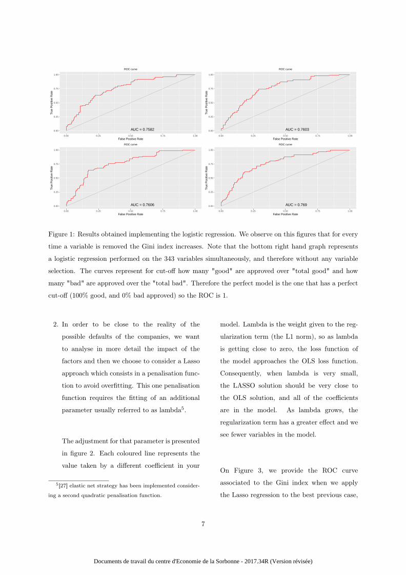
In Figure 1 we observe that the better ROC
Curve is provided for AUC= 0.7626, because it
corresponds to the best trade-off between the
"good/total good" and "bad/total bad". It is
interesting to note that the performance ob-
tained in that last case has been obtained only
with 17 variables. Thus, it is not the num-
ber of variables which is predominant but the
relevance of the variables for the objective we
have.
6
Documents de travail du centre d'Economie de la Sorbonne - 2017.34R (Version révisée)
AUC = 0.75820.00
0.25
0.50
0.75
1.00
0.00 0.25 0.50 0.75 1.00False Positive Rate
True
Pos
itive
Rat
e
ROC curve
AUC = 0.76060.00
0.25
0.50
0.75
1.00
0.00 0.25 0.50 0.75 1.00False Positive Rate
True
Pos
itive
Rat
e
ROC curve
AUC = 0.76030.00
0.25
0.50
0.75
1.00
0.00 0.25 0.50 0.75 1.00False Positive Rate
True
Pos
itive
Rat
e
ROC curve
AUC = 0.7690.00
0.25
0.50
0.75
1.00
0.00 0.25 0.50 0.75 1.00False Positive Rate
True
Pos
itive
Rat
e
ROC curve
Figure 1: Results obtained implementing the logistic regression. We observe on this figures that for every
time a variable is removed the Gini index increases. Note that the bottom right hand graph represents
a logistic regression performed on the 343 variables simultaneously, and therefore without any variable
selection. The curves represent for cut-off how many "good" are approved over "total good" and how
many "bad" are approved over the "total bad". Therefore the perfect model is the one that has a perfect
cut-off (100% good, and 0% bad approved) so the ROC is 1.
2. In order to be close to the reality of the
possible defaults of the companies, we want
to analyse in more detail the impact of the
factors and then we choose to consider a Lasso
approach which consists in a penalisation func-
tion to avoid overfitting. This one penalisation
function requires the fitting of an additional
parameter usually referred to as lambda5.
The adjustment for that parameter is presented
in figure 2. Each coloured line represents the
value taken by a different coefficient in your
5[27] elastic net strategy has been implemented consider-
ing a second quadratic penalisation function.
model. Lambda is the weight given to the reg-
ularization term (the L1 norm), so as lambda
is getting close to zero, the loss function of
the model approaches the OLS loss function.
Consequently, when lambda is very small,
the LASSO solution should be very close to
the OLS solution, and all of the coefficients
are in the model. As lambda grows, the
regularization term has a greater effect and we
see fewer variables in the model.
On Figure 3, we provide the ROC curve
associated to the Gini index when we apply
the Lasso regression to the best previous case,
7
Documents de travail du centre d'Economie de la Sorbonne - 2017.34R (Version révisée)

corresponding to AUC = 07626. Comparing
the two curves we observe that the percentages
of the "good/total good" companies versus
"bad/total bad" companies increases. Indeed,
the curve increases quickly toward 1 being
close to zero6.
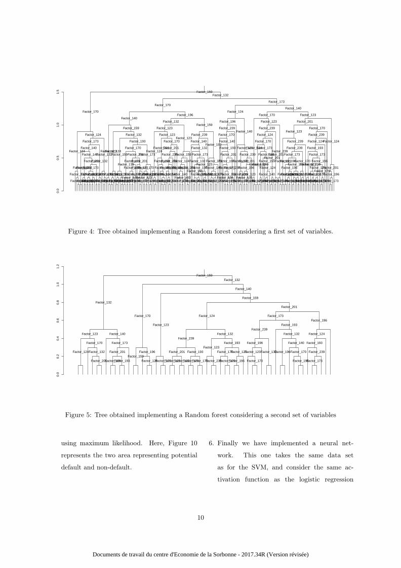
3. The third model created is a random forest. We
used all the data available as random forests are
supposed to capture linear and non linear de-
pendencies. In our case, to evaluate the prob-
ability of default of customers, the model op-
erates as a successive segmentation program.
Each variable is split in two and then reinjected
in a subsequent layer if their is some valuable
information remaining. A random forest can be
represented as the combination of a binary de-
cision tree and a bootstrap strategy. Figures 4
and 5 provide us with an illustration of the ran-
dom forest obtained considering the data used.
In Figure 5, we have used a different process
to optimize the random forest with less itera-
tions, minimizing the error at each step, thus
6in R, the function runs glmnet nfolds + 1 times; the
first to get the lambda sequence, and then the remainder to
compute the fit with each of the folds omitted. The error is
accumulated, and the average error and standard deviation
over the folds is computed. Note that cv.glmnet does NOT
search for values for alpha. A specific value should be sup-
plied, else alpha=1 is assumed by default. If users would like
to cross-validate alpha as well, they should call cv.glmnet
with a pre-computed vector foldid, and then use this same
fold vector in separate calls to cv.glmnet with different val-
ues of alpha. Note also that the results of cv.glmnet are
random, since the folds are selected at random. Users can
reduce this randomness by running cv.glmnet many times,
and averaging the error curves.
it appears more informative than what is rep-
resented in Figure 4. Once again, we observe
that it is not always when we use more vari-
ables that the best adjustment is obtained.
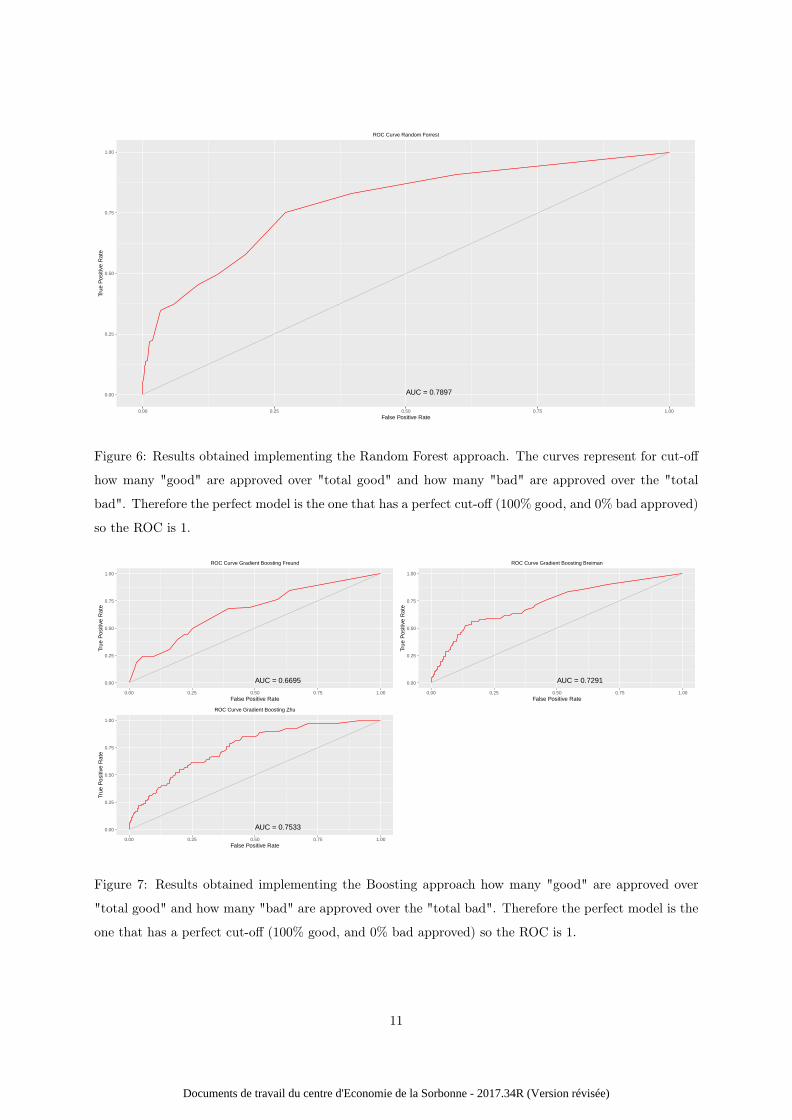
4. The next model is a random forest approach
usually referred to a boosting approach.
The difference lies in the way the learn-
ing coefficient associated to each leaf is
computed and minimized at each step of
the process. In our analysis three learn-
ing coefficient functions are compared: the
Breiman’s function, α = 12 ln
((1−err)
err
), the
Freund’s function α = ln(
(1−err)err
)and the
Zhu - SAMME algorithm implemented with
α = ln(
(1−err)err
)+ ln(nclasses − 1), where α
is the weight updating coefficient and err is
the error function as provided in [26]. For this
approach, in Figure 7 we provide the ROC
curve which still represents the impact of a
choice of a learning function over another on
the level of false positive versus true positive.
This impact is non negligible and could lead
financial institutions to a higher level of
default. Indeed, we observe that we have
increased the level of the ROC curve.
5. A Support Vector Machine approach has
been implemented. Recall that the SVM is
used here for regression purposes as it allows
scoring customers evaluating their probability
of default considering different factors. It pro-
vides a classification of the companies which
is a little different approach than the previous
approaches. Here the factors selected are once
8
Documents de travail du centre d'Economie de la Sorbonne - 2017.34R (Version révisée)

−12 −10 −8 −6
−6
−4
−2
02
4
Log Lambda
Coe
ffici
ents
75 72 55 24
1
23
56
7
10
11
13
14
1516
20
22
24
25
26
27
33
34
36
39
40
41
45
46
48
52
535455
56
59
60
61
62
64
65
66
67
69
70
71
72
73
75
77
787980
81
8284
85
87
90
9193
94
95
96
97
98
99102
103
104
105108
110
112
113
114
115
116
Figure 2: This figure represents the impact of the regularization on the coefficient and therefore the most
appropriate λ parameter.
AUC = 0.76010.00
0.25
0.50
0.75
1.00
0.00 0.25 0.50 0.75 1.00False Positive Rate
True
Pos
itive
Rat
e
ROC Curve LASSO considering all data available and splitting train and test
Figure 3: Results obtained implementing the Lasso approach. The curves represent for cut-off how many
"good" are approved over "total good" and how many "bad" are approved over the "total bad". Therefore
the perfect model is the one that has a perfect cut-off (100% goods, and 0% bads approved) so the ROC
is 1.
again different from those used in the previous
models. Indeed, the probability model for
classification fits a logistic distribution using
maximum likelihood to the decision values
of all binary classifiers, and computes the
a-posteriori class probabilities for the multi-
class problem using quadratic optimization.
The probabilistic regression model assumes
(zero-mean) Laplace-distributed errors for the
predictions, and estimates the scale parameter
9
Documents de travail du centre d'Economie de la Sorbonne - 2017.34R (Version révisée)
0.0
0.5
1.0
1.5 Factor_159
Factor_170
Factor_124
Factor_132
Factor_123
Factor_124
Factor_173
Factor_140
Factor_132
Factor_140
Factor_132
Factor_201
Factor_201
Factor_173
Factor_193
Factor_123Factor_132
Factor_124
Factor_193
Factor_170
Factor_132
Factor_239
Factor_132
Factor_132
Factor_173
Factor_132
Factor_170
Factor_140
Factor_123
Factor_193
Factor_159
Factor_124
Factor_201
Factor_140
Factor_132
Factor_159
Factor_123
Factor_196
Factor_123
Factor_239
Factor_193
Factor_170
Factor_173
Factor_193Factor_159
Factor_239
Factor_173
Factor_159
Factor_140Factor_173
Factor_196
Factor_201
Factor_173
Factor_239
Factor_193
Factor_173
Factor_170
Factor_123Factor_123
Factor_124
Factor_124
Factor_196
Factor_132
Factor_123
Factor_124
Factor_159
Factor_140
Factor_123
Factor_201
Factor_159
Factor_193
Factor_124
Factor_159Factor_132
Factor_170
Factor_201
Factor_239
Factor_239
Factor_132
Factor_140
Factor_193
Factor_124
Factor_123
Factor_159
Factor_124
Factor_201
Factor_140
Factor_173Factor_193
Factor_239
Factor_124
Factor_159
Factor_239
Factor_140
Factor_132
Factor_173
Factor_132
Factor_196
Factor_201
Factor_193
Factor_123
Factor_123
Factor_123
Factor_170
Factor_124
Factor_193
Factor_173
Factor_140
Factor_124
Factor_123
Factor_170
Factor_201
Factor_173
Factor_124
Factor_196
Factor_239
Factor_170
Factor_140
Factor_193
Factor_201
Factor_193
Factor_170
Factor_196Factor_123
Factor_196
Factor_239
Factor_123
Factor_140
Factor_123
Factor_170
Factor_239
Factor_196
Factor_239
Factor_201
Factor_196
Factor_170Factor_123
Factor_196
Factor_140
Factor_170
Factor_124
Factor_123
Factor_123
Factor_239
Factor_124
Factor_170
Factor_140
Factor_173
Factor_159
Factor_140
Factor_196
Factor_159
Factor_124
Factor_140
Factor_170
Factor_201
Factor_196
Factor_201
Factor_123
Factor_239
Factor_193
Factor_123
Factor_201
Factor_123
Factor_159
Factor_239
Factor_239
Factor_173
Factor_196
Factor_124
Factor_196
Factor_124
Factor_124
Factor_159
Factor_124
Factor_196
Factor_124
Factor_196
Factor_170
Factor_170
Factor_196
Factor_170
Factor_239
Factor_124
Factor_193
Factor_123
Factor_196
Factor_173
Factor_239
Factor_196
Factor_124
Factor_196
Factor_124
Factor_170
Factor_123
Factor_170
Factor_239
Factor_124
Factor_201
Factor_196
Factor_173
Figure 4: Tree obtained implementing a Random forest considering a first set of variables.
0.0
0.2
0.4
0.6
0.8
1.0
1.2
Factor_159
Factor_132
Factor_123
Factor_124
Factor_170
Factor_132
Factor_201
Factor_140
Factor_173
Factor_201
Factor_159Factor_193
Factor_132
Factor_170
Factor_159Factor_196
Factor_124
Factor_140
Factor_123
Factor_170
Factor_159
Factor_124
Factor_239
Factor_201
Factor_123Factor_132
Factor_193
Factor_173Factor_173
Factor_132
Factor_123
Factor_239
Factor_193
Factor_170
Factor_170
Factor_123
Factor_196
Factor_201
Factor_173
Factor_239
Factor_196
Factor_123
Factor_170
Factor_132
Factor_193
Factor_132
Factor_196
Factor_140
Factor_170
Factor_196
Factor_196
Factor_124
Factor_193
Factor_239
Factor_173
Figure 5: Tree obtained implementing a Random forest considering a second set of variables
using maximum likelihood. Here, Figure 10
represents the two area representing potential
default and non-default.
6. Finally we have implemented a neural net-
work. This one takes the same data set
as for the SVM, and consider the same ac-
tivation function as the logistic regression
10
Documents de travail du centre d'Economie de la Sorbonne - 2017.34R (Version révisée)
AUC = 0.78970.00
0.25
0.50
0.75
1.00
0.00 0.25 0.50 0.75 1.00False Positive Rate
True
Pos
itive
Rat
e
ROC Curve Random Forrest
Figure 6: Results obtained implementing the Random Forest approach. The curves represent for cut-off
how many "good" are approved over "total good" and how many "bad" are approved over the "total
bad". Therefore the perfect model is the one that has a perfect cut-off (100% good, and 0% bad approved)
so the ROC is 1.
AUC = 0.66950.00
0.25
0.50
0.75
1.00
0.00 0.25 0.50 0.75 1.00False Positive Rate
True
Pos
itive
Rat
e
ROC Curve Gradient Boosting Freund
AUC = 0.75330.00
0.25
0.50
0.75
1.00
0.00 0.25 0.50 0.75 1.00False Positive Rate
True
Pos
itive
Rat
e
ROC Curve Gradient Boosting Zhu
AUC = 0.72910.00
0.25
0.50
0.75
1.00
0.00 0.25 0.50 0.75 1.00False Positive Rate
True
Pos
itive
Rat
e
ROC Curve Gradient Boosting Breiman
Figure 7: Results obtained implementing the Boosting approach how many "good" are approved over
"total good" and how many "bad" are approved over the "total bad". Therefore the perfect model is the
one that has a perfect cut-off (100% good, and 0% bad approved) so the ROC is 1.
11
Documents de travail du centre d'Economie de la Sorbonne - 2017.34R (Version révisée)

ROC Curve: Boosting models
False positive rate
True
pos
itive
rat
e
0.0 0.2 0.4 0.6 0.8 1.0
0.0
0.2
0.4
0.6
0.8
1.0
Freund ModelZhu ModelBreiman Model
Figure 8: This figure allow comparing boosting approaches. The methodology is similar to the random
forest. The difference is that it works to reduce the error at each step of the process. We compare
three learning coefficient functions: Breiman’s function, Freund’s function and Zhu’ SAMME algorithm
is implemented with α = ln(
(1−err)err
)+ ln(nclasses− 1)
AUC = 0.57560.00
0.25
0.50
0.75
1.00
0.00 0.25 0.50 0.75 1.00False Positive Rate
True
Pos
itive
Rat
e
ROC Curve Support Vector Machine
Figure 9: Results obtained implementing the Support Vector Machine approach how many "good" are
approved over "total good" and how many "bad" are approved over the "total bad". Therefore the perfect
model is the one that has a perfect cut-off (100% good, and 0% bad approved) so the ROC is 1.
though in that case the way the factors are
combined within the hidden layer is differ-
ent. Indeed, the weights associated to the
factors considered in the learning is different,
therefore it naturally results in a different
set of outcomes. The ROC associated to the
12
Documents de travail du centre d'Economie de la Sorbonne - 2017.34R (Version révisée)

01
0 100 200 300 400
0.1
0.2
0.3
0.4
o
o
o
o
o
o
oo
o
oo
oo
o
o ooo
o
o
o
o
ooo
o
o
oo
o
o
o
o
o
oo
o
o
o
o
o
o
o
o
o
o
o
o
oo
o
o
o
o
o
o
oo
o
oo
o
o
o
ooo
o
o
o
oo
o
o
o
o
o
o
oo
o
o
o
o
oo
oo
o
oo o
oo
o
o
oo
oo
o
oo
o
oo
o
o
o
o
o
o
o o
o
oo
o
o
o
o
o
o
oo
oo
o
o
o o
o
o
o
o
o
o
o
ooo
ooo
oo
o
o
o
o
o
oo
o
o
o
o
o
o
o
o
o
o
o
o
o
o
o
o o
o
o
oo
o
oo
oo
o
o
oo
oo ooo oooo
oooooo
ooooo
oo
oooox
x
x xx
x
x xxx
x
x
x
x
xxx
xx
x
x
xx
x
xxx
x
xx
xx xxx
xxx
x
x
x
x
xx x
x
x
x
x
xx
x
x
x x
x
x
x
x
xx
x
x
xxx
xx
x
xx
x
xx
x
x x
x
x
xx
xx
x
x
xxxx xx
xxx
x
x
x
xxx
xx
x
x
xxx
x x
x
x
x
xx x
xx
x
xx
x
xx
xx
x
xxx
x
x
x xx
x xx
x
xx
xx
x
x
x
x
xx
x
x
xx
x
x
x
x
xx
x
xx
xx
xxx x
x
x
x
x xxx
xx
x x
xxxxx
x
x
x
xx
xxx
xx
x
x
xxx
xx
xx xx
x
x
xx xx x
x
x
xx
xx x xx
x
xx
x x
xxx
x
xx
xxxx x
x
xx
xxx x
x
x
x
x
xx
x
x
x xx
xx
xx x
x
x
xx
xxx
x
xx
x
x
x
xx
x
xxx x
x
xxxx
x
xxx
xxxx x
x
x
xx
xxx
xxxx
xxx xxx
x
xx x
x
x xx
x
xx
xx
xx
x
xx
x
x
x xx xx
x
x
x
x
xx
xx
xx x
xx
x
x xx
x
x
x
x
x
xx
xxxx
x
x
x
x
x
x
x
x
x
x
xxx
x
xx
xx
x x xx
x
xx
x
x
x
x
xx
x
x
xx xxx x
xx
x
x xx
x
x
xx
x
x
x
x
x
xx
xxx
xx
x
x
x
x
x xx
x
x
x
x
xx
xx xxxxx
x
x
x
x x xx
x
x
x
x x
x
x
x
x xx
x
x x
xx
xxx
x
x
x
x
x
x
x
x
x
x
x
x
x
x
x
x x xx x
x
x xxxx x
x
xxx
x
xx
x
xx
x
xxxxxx
xxx xxxxx
xx xxx
xxxxxxx
xxx
xxx
x x xx
xxxxx xxxxxxxxxxxx
xxxx
xxxxxxxxxxx
xx x
x
xxxx x
xxxxx
xxxxx
xxxx xx
xxxx
x
xxxx
xxxxxx
xxxxx
xxxxxx xx xx
xxxxxx
xxxxx xxx
xxx
xx
xxxx xx
x xxxxxxxxxxxxx
xxxx
xxxxx xxx
xxxx
xxxxx
xxxx
xxxx
xxxx xxxxx x
xxxxx xxx
xxxxxxxxx
xxxxx
x
xx
xxxxxx
xx
xxxxxxxxx
x xx xxxxxxx
xxxx
xx
xxx xxxx
xxxxxx
xxx
xxx xx
xxx
x xx
xxxx
x
xx
xxxxx
xxxxx
xxxx
xxxxx
xxxxxxxx
xxxx
xxxx x xxxxx xxxxx
xxxxxxx xxx x
xxxx
xxx
xxxxxxx
xx
xxxxx
xxxx
xxxxx
xx xxxxxxxxxx
xxxxxxx
xxxx
x
xxx
xxxxxxx
x
xxxxx
xxxxxxxx
xxxx
xxxxxxxxx
xxx xxxxx
xxxxxxxx xxx
xx
xx
xxxx xxxxx
xx
xx
xxx xx
xx
xxx
xxxxxxxxxxx
xxxx
xxx
SVM classification plot
Factor_52
Fact
or_4
2
Figure 10: This figure illustrates the SVM methodology, which in our case provides us with the worst
adjustment results.
Neural Network approach is given in Figure 11.
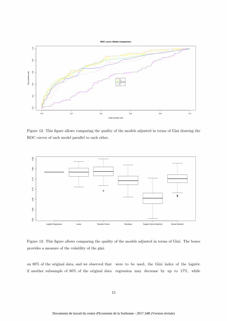
7. In Figure 12, the ROC curve of each model
analysed have been plotted. These curves once
translated in terms of AUC, confirm that the
Random Forest is the best approach with an
AUC equal to 0.7897, followed by the Logistic
Regression with a best AUC equal to 0.769, fol-
lowed by a LASSO approach with an AUC of
0.76.1, followed by a Boosting approach with a
best AUC of 0.7533 obtained using the Zhu’s
error function, followed by the Neural Network
approach giving an AUC of 0.6906 and the Sup-
port Vector Machine approach comes last with
an AUC of 0.5756. Besides, we provide in Fig-
ure 13 a way to compare the 6 different mod-
ellings computing the variance of the Gini in-
dex and its level of randomness, except for the
logistic regression. On this figure we observe
that in average, the Random Forest offers a
better explanatory power relying on a larger
number of variable, however, the improvement
offered by the random forest compared to the
logistic regression is not very large. Indeed,
the logistic regression relies on a subset of the
pool of variables used for the Random Forest.
However, if we draw a parallel between this
figure and the first one presented in that sec-
tion, we may conclude that these results are
only valid considering the current data set. In-
deed, the first figure tells us that considering
the set of data approved months ago does not
provide the best adjustment as randomly re-
moving some variables leads to better Gini in-
dexes, while using the full set of 343 variables
leads to an improvement as soon as a random
13
Documents de travail du centre d'Economie de la Sorbonne - 2017.34R (Version révisée)

AUC = 0.69060.00
0.25
0.50
0.75
1.00
0.00 0.25 0.50 0.75 1.00False Positive Rate
True
Pos
itive
Rat
e
ROC Curve Neural Network
Figure 11: Results obtained implementing a Neural Network approach showing how many "good" are
approved over "total good" and how many "bad" are approved over the "total bad". Therefore the perfect
model is the one that has a perfect cut-off (100% good, and 0% bad approved) so the ROC is 1.
forest is selected. This statement leads us to
the conclusion that if the data sets and the
types of variables change (for example using
unstructured data), the order of the models
may change again.
Considering the results presented in the previous
section, it is interesting to note that though all
the models could be used to achieve the same
tasks, the way to perform the computations are
not identical and do not philosophically imply
the same thing. Indeed, though for the logistic
regression, the data has been selected such that
no correlations are present, the other models do
not necessarily require that. The random forest
strategies have the capability to capture non-linear
dependencies, while neural networks are entirely
based on building and capturing relationships
between variables.
Furthermore, these results have been obtained on a
static data set; therefore the evolution of the data
set may lead to a different ranking of the models.
Indeed, here though random forests seems in aver-
age better than the others, this is not necessarily
the same if the data set were to evolve. Besides,
we do not know yet how the integration of other
data sources (such as integration of social medias)
would impact this ranking, however, considering
the nature of the models, we are inclined to think
that neural networks or random forests would be
more appropriate than the others.
Finally, it is interesting to note that Figure 13 has
been obtained considering a single sample based
14
Documents de travail du centre d'Economie de la Sorbonne - 2017.34R (Version révisée)
ROC curve: Model comparison
False positive rate
True
pos
itive
rat
e
0.0 0.2 0.4 0.6 0.8 1.0
0.0
0.2
0.4
0.6
0.8
1.0
ALRLassoRandom ForestBoosting ModelSVMNN
Figure 12: This figure allows comparing the quality of the models adjusted in terms of Gini drawing the
ROC curves of each model parallel to each other.
●
●●
Logistic Regression Lasso Random Forest Boosting Support Vector Machine Neural Network
0.55
0.60
0.65
0.70
0.75
0.80
0.85
Figure 13: This figure allows comparing the quality of the models adjusted in terms of Gini. The boxes
provides a measure of the volatility of the gini.
on 80% of the original data, and we observed that
if another subsample of 80% of the original data
were to be used, the Gini index of the logistic
regression may decrease by up to 17%, while
15
Documents de travail du centre d'Economie de la Sorbonne - 2017.34R (Version révisée)

for other approaches, the results would still be
contained in the confidence intervals of the box
plots. This observation may greatly impact the
original ranking disclosed in this paper. We have
also observed that the selection of the activation
function, the algorithms embedded within the
machine learning approaches presented, and the
index used to evaluate the quality of the models
may lead to different results too. Therefore, this
point should be carefully handled.
From both lenders and financial institutions cus-
tomers point of view, the main issue lies in the fact
that ultimately a loan will be provided or not, over-
charged or not and therefore an inaccurate credit
score might have a tremendous impact in companies
lives-cycles. This statement has to be moderated by
the fact that models are usually following an intense
governance process, therefore only border line com-
panies might be impacted. Indeed, the managers
are allowed to select the acceptable level of false
positive (see the successive ROC curve presented
above). These models are supposed to be action-
able. The main issue is that these companies con-
sidered as riskier by banks might also be those gen-
erating the highest margins. To summarise, with an
inappropriate credit scoring models, some compa-
nies may not develop themselves and therefore may
not be able to participate to the global economy
and in counterpart banks may not be generating
the largest income possible.
4 Conclusion and further dis-
cussion
First and foremost, the data used have been
collected and provided by a financial institution,
and our analysis uses as a benchmark the model
used by the financial institution and approved by
the regulator. As such the data have not been re-
processed. Consequently, following [4] it seems that
the question of actionability may need to be even
further addressed, i.e. looking for relevant patterns
that really support knowledge discovery. Indeed,
a model supporting a meaningful decision making
process leads to results actually representative of a
risk of default. Though some factors are tradition-
ally considered as able to characterise a default,
we observe that the patterns might no be complete
and therefore the results might not always be as
actionable as we think as the score might be biased.
Consequently the traditional information set may
need to be enlarged, for example as mentioned
before, considering non structured data. Note that
digital finance companies or fintechs such as online
lenders uses alternative data sources to calculate
the creditworthiness of borrowers, but in that case
they are also having blind spots, as they may not
capture companies banking behaviours.
Another dramatic issue in our case is related to
the stationarity of the data. As discussed in the
previous section, we observe that the models used
are more sensitive to the non stationary behaviour
of the data. Indeed, when the data used for fitting
have not the same properties of the data used
for testing (because the statistical moments are
16
Documents de travail du centre d'Economie de la Sorbonne - 2017.34R (Version révisée)

different, for instance), the result will be biased
or completely erroneous. As a corollary of not
being stationary, data are not necessarily IID when
most models tested are assuming IID inputs and
as such most models might be inadequate or have
a reduced durability. Here, the consideration of
X-intelligence approach might provide a reliable
solution ([6]).
As we have shown in Section 3, the choice of the
models is not naive, nor was the choice of the
indicator we chose to have as an answer to our
objective. This exercise points to a number of
questions that will be the purpose of companion
papers. If it appears necessary to compare different
models to a given data set, this exercise would
be even more relevant considering a larger data
set and considering data coming from alternative
sources. Indeed, with a larger number of data
points, naturally containing more information,
more dependence, some non linearity and specific
features like trends, seasonalities and so on, should
lead to more relevant outcomes, as well as poten-
tially controversial questions. The choice of the
indicator to retain the "best " model is also very
difficult when we base our modelling on machine
learning: it is important to know exactly what are
the underlying processes for automation to under-
stand the specific features we retain, the question
of the number of iterations is also important to get
a form of convergence, and what convergence. This
point is also important to discuss.
Using linear modellings is not sufficient to take
into account the existence of specific features such
as strong dependence. Another question is to know
exactly the error we measure with this kind of
modelling, are we close to a type 1 or a type 2
error? The application we provide gives a picture
at time t of the capability of companies to obtain
a loan or not based on their creditworthiness,
therefore an important question is how to inte-
grate new pieces of information in these procedures.
While the regulation and the legislation related to
big data is still embryonic, the implementation of
machine learning models has to be carefully done
as the dynamic philosophy implied cannot yet prop-
erly be handled by the current static regulation and
internal governance ([21]). Therefore, this thought-
ful process leads to questions concerning regulators.
There is a strong possibility of risk materialisation
depending on the chosen models; the attitude of the
regulator - historically when dealing with the risk
topic - is to be conservative or close to a form of
uniformity. This posture seems complicated with
Big Data as the emergence of continuous flows me-
chanically prevents imposing the same model to all
institutions. Dynamics need to be introduced, and
it is not simple. We point out the fact that, even
if all the models used are very well known in the
non-parametric statistics, these dynamics need to
be clearly understood for the use they provide. Fur-
thermore, target specifications and indicators need
to be put in place in order to avoid large approxi-
mations and bad results.
17
Documents de travail du centre d'Economie de la Sorbonne - 2017.34R (Version révisée)

References
[1] A. Ben-Hur, D. Horn, H. Siegelmann, and
V. Vapnik. Support vector clustering. Jour-
nal of Machine Learning Research, 2:125–137,
2001.
[2] Jean-François Boulicaut and Jérémy Besson.
Actionability and formal concepts: A data
mining perspective. Formal Concept Analysis,
pages 14–31, 2008.
[3] L. Breiman. Bagging predictors. Machine
Learning, 24(2):123–140, 1996.
[4] Longbing Cao. Actionable knowledge discovery
and delivery. Wiley Int. Rev. Data Min. and
Knowl. Disc., 2(2):149–163, March 2012.
[5] Longbing Cao. Data science: a comprehensive
overview. ACM Computing Surveys (CSUR),
50(3):43, 2017.
[6] Longbing Cao. Data science: Challenges
and directions. Communications of the ACM,
60(8):59–68, 2017.
[7] Le Chang, Steven Roberts, and Alan Welsh.
Robust lasso regression using tukey’s biweight
criterion. Technometrics, (just-accepted),
2017.
[8] Dunren Che, Mejdl Safran, and Zhiyong Peng.
From big data to big data mining: challenges,
issues, and opportunities. In International
Conference on Database Systems for Advanced
Applications, pages 1–15. Springer, N.Y., 2013.
[9] CL Philip Chen and Chun-Yang Zhang. Data-
intensive applications, challenges, techniques
and technologies: A survey on big data. In-
formation Sciences, 275:314–347, 2014.
[10] B. deVille. Decision Trees for Business Intelli-
gence and Data Mining: Using SAS Enterprise
Miner. SAS Press, Cary (NC), 2006.
[11] Gerard George, Martine R Haas, and Alex
Pentland. Big data and management. Academy
of Management Journal, 57(2):321–326, 2014.
[12] Corrado Gini. On the measure of concentration
with special reference to income and statistics.
Colorado College Publication, General Series,
208:73–79, 1936.
[13] James A Hanley and Barbara J McNeil. The
meaning and use of the area under a receiver
operating characteristic (roc) curve. Radiology,
143(1):29–36, 1982.
[14] Bertrand K Hassani. Artificial neural network
to serve scenario analysis purposes. In Scenario
Analysis in Risk Management, pages 111–121.
Springer, 2016.
[15] T. Hastie, R. Tibshirani, and J. Friedman. The
Elements of Statistical Learning: Data min-
ing,Inference,and Prediction. Springer, New
York, 2009.
[16] Timothy E Hewett, Kate E Webster, and
Wendy J Hurd. Systematic selection of key
logistic regression variables for risk prediction
analyses: A five-factor maximum model. Clin-
ical Journal of Sport Medicine, 2017.
[17] Adam Jacobs. The pathologies of big data.
Communications of the ACM, 52(8):36–44,
2009.
18
Documents de travail du centre d'Economie de la Sorbonne - 2017.34R (Version révisée)

[18] Amod Jog, Aaron Carass, Snehashis Roy,
Dzung L Pham, and Jerry L Prince. Random
forest regression for magnetic resonance image
synthesis. Medical image analysis, 35:475–488,
2017.
[19] Miroslav Kubat. Artificial neural networks. In
An Introduction to Machine Learning, pages
91–111. Springer, 2017.
[20] David Lazer, Ryan Kennedy, Gary King, and
Alessandro Vespignani. The parable of google
flu: traps in big data analysis. Science,
343(6176):1203–1205, 2014.
[21] Neha Mathur and Rajesh Purohit. Issues and
challenges in convergence of big data, cloud
and data science. International Journal of
Computer Applications, 160(9), 2017.
[22] Gene Neyer. Next generation payments: Al-
ternative models or converging paths? Journal
of Payments Strategy & Systems, 11(1):34–41,
2017.
[23] Zhiyuan Shi, Parthipan Siva, and Tao Xiang.
Transfer learning by ranking for weakly su-
pervised object annotation. arXiv preprint
arXiv:1705.00873, 2017.
[24] Shan Suthaharan. Support vector machine.
In Machine Learning Models and Algorithms
for Big Data Classification, pages 207–235.
Springer, 2016.
[25] Robert Tibshirani. Regression shrinkage and
selection via the lasso. Journal of the Royal
Statistical Society. Series B (Methodological),
pages 267–288, 1996.
[26] Ji Zhu, Hui Zou, Saharon Rosset, Trevor
Hastie, et al. Multi-class adaboost. Statistics
and its Interface, 2(3):349–360, 2009.
[27] Hui Zou and Trevor Hastie. Regularization and
variable selection via the elastic net. Journal
of the Royal Statistical Society: Series B (Sta-
tistical Methodology), 67(2):301–320, 2005.
19
Documents de travail du centre d'Economie de la Sorbonne - 2017.34R (Version révisée)