relativistic algorithm for time transfer in mars missions …€¦ · · 2015-01-15relativistic...

RAA 2015 Vol. 15 No. 2, 281–292 doi: 10.1088/1674–4527/15/2/011http://www.raa-journal.org http://www.iop.org/journals/raa

Research inAstronomy andAstrophysics

Relativistic algorithm for time transfer in Mars missions underIAU Resolutions: an analytic approach ∗

Jun-Yang Pan1 and Yi Xie1,2

1 School of Astronomy and Space Science, Nanjing University, Nanjing 210093, China;[email protected]

2 Key Laboratory of Modern Astronomy and Astrophysics, Nanjing University, Ministry ofEducation, Nanjing 210093, China

Received 2014 May 4; accepted 2014 June 12

Abstract With tremendous advances in modern techniques, Einstein’s general rela-tivity has become an inevitable part of deep space missions. We investigate the rela-tivistic algorithm for time transfer between the proper time τ of the onboard clock andthe Geocentric Coordinate Time, which extends some previous works by includingthe effects of propagation of electromagnetic signals. In order to evaluate the implicitalgebraic equations and integrals in the model, we take an analytic approach to workout their approximate values. This analytic model might be used in an onboard com-puter because of its limited capability to perform calculations. Taking an orbiter likeYinghuo-1 as an example, we find that the contributions of the Sun, the ground stationand the spacecraft dominate the outcomes of the relativistic corrections to the model.

Key words: reference systems — time — method: analytical — space vehicles

1 INTRODUCTION

With tremendous advances in modern techniques, Einstein’s general relativity (GR) has become aninevitable part of deep space missions. It has gone far beyond theoretical astronomy and physics intopractice and engineering (Nelson 2011). Effects due to GR clearly showed up in the radio signals ofsome space missions (e.g. Bertotti et al. 2003; Jensen & Weaver 2007), which provide the tightestconstraint on GR (Bertotti et al. 2003). However, Kopeikin et al. (2007) pointed out that the testof GR by the Cassini spacecraft (Bertotti et al. 2003) is under a restrictive condition that the Sun’sgravitational field is static, and if this restriction is removed the test becomes less stringent.

In GR, one important idea is to abandon the concept of Newton’s absolute time. There existdifferent kinds of times: proper time and coordinate times (Misner et al. 1973; Landau & Lifshitz1975). Theoretically, the readings of an ideal clock form the proper time τ , which is an observableand is associated with the clock itself. In fact, there is not an ideal clock. An atomic clock approachesan ideal clock with some finite error. However, even if an atomic clock were ideal, we still have tohypothesize that it reads the proper time. This is because GR is a geometric theory but an atomic

∗ Supported by the National Natural Science Foundation of China.

282 J. Y. Pan & Y. Xie

clock is a quantum mechanical device, not governed by geometry but by the laws of quantum me-chanics, which are still not geometrized. The coordinate times cannot be measured directly, but theymight be used as variables in the equations of motion of celestial and artificial bodies and lightrays. Coordinate times are connected with the proper time through the four-dimensional space-timeinterval, whose mathematical expression depends on kinematics and dynamics of the clock. Thisdramatically changes the way clocks are synchronized and the associated time transfer (see Petit &Wolf 2005; Nelson 2011, for reviews and refereces therein). Experiments involving time/frequencytransfer might be used for testing theories of gravity (e.g. Samain 2002; Cacciapuoti & Salomon2009; Wolf et al. 2009; Christophe et al. 2009, 2012; Deng & Xie 2013a,b, 2014).

In exploration missions to Mars and other planets, synchronization between the clock onboarda spacecraft and a clock on the ground is critical for control, navigation and scientific operation.According to International Astronomical Union (IAU) Resolutions (Soffel et al. 2003), two interme-diate steps are required. Step 1 is to relativistically transform onboard τ to the Barycentric CoordinateTime (TCB), which is the global time of the solar system. Then, in Step 2, TCB is converted to theGeocentric Coordinate Time (TCG), which is the coordinate time belonging to the local referencesystem of the Earth. Then, TCG can be easily changed to other time scales associated with Earth,such as Terrestrial Time (TT), International Atomic Time (TAI) and Coordinated Universal Time(UTC).

Taking the Yinghuo-1 mission (Ping et al. 2010a,b) as a technical example of future ChineseMars explorations, some works have been devoted to investigating Step 1 and Step 2. Deng (2012)studied the transformation of Step 1 by analytic and numerical methods and found two main ef-fects: the gravitational field of the Sun and the velocity of the spacecraft in the Barycentric CelestialReference System (BCRS). The combined contribution of these two effects can reach a few sub-seconds in one year (Deng 2012). Pan & Xie (2013) took clock offset into account in Step 1 andfound that if an onboard clock can be calibrated to achieve an accuracy better than ∼10−6 − 10−5 sin one year (depending on the type of clock offset), the relativistic transformation between τ andTCB will need to be carefully handled. Pan & Xie (2014) investigated the relativistic transformationbetween τ and TCG, which combines Step 1 and Step 2. It was found that the difference between τand TCG can reach the level of about 0.2 seconds in a year and if the threshold of 1 microsecond(µs) is adopted, this transformation must include the effects due to the Sun, Venus, the Moon, Mars,Jupiter, Saturn and the velocities of the spacecraft and the Earth.

In this paper, we will include the effects of light propagation in the relativistic algorithm of timetransfer for Mars missions under IAU Resolutions. More specifically, the relativistic time transferconnecting two time scales is carried out by the transmission of electromagnetic signals, whichmight be encoded with necessary information and commands. This also means the time scale inthe present work is about 103 seconds, which is the light propagation time from a ground stationto a Mars orbiter. The effects of the propagation of signals are absent in the previous works (Deng2012; Pan & Xie 2013, 2014) and the time scale of one year in these works is much longer thanthe one we focus on here. For an orbiter around Mars, which has an orbit like Yinghuo-1’s, we willdevelop an analytic model for such a procedure of time transfer. This analytic approach means allof the algebraic equations and integrals in the model will be solved and evaluated in some wayswith sufficient approximations. Such an algorithm might be adopted for an onboard processor withlimited capability to perform computation. The validity of this analytic approach needs to be checkedindependently and such a check will be our next goal.

In Section 2, we will establish a general model of relativistic time transfer between τ and TCGfor a Mars orbiter according to IAU Resolutions (Soffel et al. 2003). This model includes the effectsof signal transmission from a station to a spacecraft. Implicit algebraic equations and integrals inthe model will be approximately solved and evaluated in Section 3. In Section 4, by assuming anYinghuo-1-like mission, we will calculate and show the contributions from various sources in thisanalytic model. Conclusions and discussion will be presented in Section 5.

Relativistic Algorithm of Time Transfer for Mars Missions 283

2 GENERAL MODEL OF TIME TRANSFER BETWEEN τ AND TCG

In the framework of IAU Resolutions (Soffel et al. 2003), a clock onboard an orbiter (hereafter “P”)around Mars measures its own proper time τ and a station (hereafter “S”) on the surface of theEarth can have its coordinate time T in TCG, which can be calculated from other well-maintainedtime scales, such as TT. In order to synchronize the onboard τ with T on the Earth, S emits anelectromagnetic signal encoded with some necessary information at time tE in TCB and P receivesthe signal at time tR in TCB. In this context, we can find the relation between these times as (e.g.Kopeikin et al. 2011)

dτ

dT=

dτ

dtR

dtRdtE

dtEdT

, (1)

where the first term describes the transformation between τ and TCB, the second term accounts forthe propagation of the electromagnetic signal from S to P and the third term is the transformationbetween TCB and TCG.

The relativistic 4-dimensional transformation between τ and the TCB in Equation (1) reads as(Soffel et al. 2003)

dτ

dtR= 1− ε2

[U(xP) +

12v2

P

]+O(ε4) . (2)

Here, ε = c−1 and c is the speed of light. U(xP) is the Newtonian gravitational potential evaluated atthe position of the spacecraft xP and vP is the velocity of the spacecraft in the BCRS. The potentialcan be decomposed further as U =

∑A UA, where the index “A” enumerates each body whose

gravitational effect needs to be considered. Focusing on a spacecraft like Yinghuo-1, Deng (2012)and Pan & Xie (2013) studied its effects on the time transfer. The relativistic transformation betweenTCB and TCG in Equation (1) is (Soffel et al. 2003)

dtEdT

= 1 + ε2{

U(x⊕) +12v2⊕ +

ddT

[v⊕ · (xS − x⊕)

]}+O(ε4) , (3)

where xS and x⊕ are respectively the positions of the station and the geocenter in the BCRS andboth of them are functions of tE.

The second term in Equation (1), which describes the propagation of the signal, can be obtainedfrom the relativistic light ray equations (see chap. 7 in Kopeikin et al. 2011, for details) and, thus,we can have (Moyer & Yuen 2000; Kopeikin et al. 2011)

∆t ≡ tR − tE = ∆t1 + ∆t2 +O(ε4) , (4)

where

∆t1 ≡ εf1 = ε|xP(tR)− xS(tE)| , (5)

∆t2 ≡ ε3f2 = 2ε3G∑

A

mA ln[rRA + n · rRA

rEA + n · rEA

]. (6)

Here, ∆t1 is the Euclidean geometric effect and ∆t2 is the Shapiro time delay (Shapiro 1964). Interms of ∆t1, xP and xS depend respectively on tR and tE. In terms of ∆t2, we ignore the motionsof all the gravitational bodies. Such a treatment is only valid when the time scale of light propagationis much less than the time scales of orbital motions of celestial bodies. This condition is satisfied inour investigation of a Mars mission because the light propagation time from S to P is at the levelof ∼103 s, which is much shorter than the time scales of planetary motions. In the case that time-dependent gravitational fields can no longer be neglected, a profound and systematic approach tointegrating the light ray equations has been worked out (Kopeikin 1997; Kopeikin & Schafer 1999;Kopeikin & Mashhoon 2002; Kopeikin et al. 2006; Kopeikin & Makarov 2007; Kopeikin 2009). In


the Shapiro term (6), the index “A” enumerates each body whose gravitational effect needs to beconsidered. rA, rA and n are quantities associated with the propagation of the signal and they are

n =xP(tR)− xS(tE)|xP(tR)− xS(tE)| , (7)

rA(t) = xS(tE)− xA(tE) + cn(t− tE) +O(ε2) , (8)

andrEA = rA(tE), rEA = |rA(tE)|, rRA = rA(tR), rRA = |rA(tR)| . (9)

Therefore, differentiating (4) and combining it with Equations (2) and (3), we can expressEquation (1) as

dτ

dT= 1 + ε

df1

dtE+ ε2

(1 + ε

df1

dtE

){U(x⊕) +

12v2⊕ +

ddT

[v⊕ · (xS − x⊕)

]}

−ε2(

1 + εdf1

dtE

)[U(xP) +

12v2

P

]+ ε3

df2

dtE+O(ε4) . (10)

After integrating it, we can eventually obtain that

τ − T = ∆t + ∆T + ∆τ +O(ε4) . (11)

Here, ∆t is the light time solution accounting for propagation of the signal (Moyer & Yuen 2000;Kopeikin et al. 2011). ∆T is the transformation between TCG and TCB at S and it has two compo-nents, ∆T = ∆T1 + ∆T2, where ∆T1 and ∆T2 are respectively associated with the positions andvelocities of the geocenter and S. Their expressions are

∆T1 = ε2∫ tR

tE

[U(x⊕) +

12v2⊕

]dt , (12)

∆T2 = ε2v⊕(tE) ·[xS(tE)− x⊕(tE)

]. (13)

The term ∆τ is the transformation between TCB and τ at P and has the form

∆τ = −ε2∫ tR

tE

[U(xP) +

12v2

P

]dt . (14)

By making use of Equation (11), one might carry out time transfer between the times onboardand on the Earth by the transmission of signals. However, in practice, some mathematical worksneed to be done: one is to solve for ∆t from the implicit algebraic Equation (4) and the other isto evaluate the integrals in Equations (12) and (14). They can be worked out in either a numericalor analytic way (e.g. Fukushima 2010). In the present paper, we will adopt an analytic way basedon some approximations to handle them. Although the validity of these approximations has to bechecked independently, this approach might be used by an onboard computer because of its limitedcapability to perform calculations.

3 ANALYTIC APPROACH FOR THE MODEL

Equation (4) is an implicit algebraic equation of tR and tE. Taking a quick estimation, we find that,for an orbiter around Mars, ∆t1 on the right-hand side of Equation (4) is at the level of ∼103 s and∆t2 is about 10−5 s due to the largest contribution from the Sun, i.e. ∆t2/∆t1 ∼ 10−8, which meansthe leading term of Equation (4) is

∆t ≡ tR − tE ≈ ∆t1 = ε|xP(tR)− xS(tE)| . (15)


Depending on the procedure for the time transfer, we can generally write the above equation as

∆t1 = ε|xP(tE + ∆t1)− xS(tE)|+O(ε∆t2) , (16)

or∆t1 = ε|xP(tR)− xS(tR −∆t1)|+O(ε∆t2) . (17)

If ∆t1 is much less than the time scale of the motion of P, Equation (16) can be Taylor expanded as

xP(tE + ∆t1) = xP(tE) + vP(tE)∆t1 +12aP(tE)∆t21 +O(∆t31) . (18)

Similarly, if ∆t1 is much less than the time scale of the motion of S, Equation (17) can be ex-panded as

xS(tR −∆t1) = xS(tR)− vS(tR)∆t1 +12aS(tR)∆t21 +O(∆t31) . (19)

Substituting Equations (18) and (19) into (16) and (17) respectively, we can solve them respectivelyby iteration as

∆t1 = ε rPS(tE) + ε2rPS(tE) · vP(tE) +12ε3

{v2

P(tE) rPS(tE)

+[rPS(tE) · aP(tE)

]rPS(tE) +

[rPS(tE) · vP(tE)

]2

r−1PS (tE)

}+O(ε4) , (20)

where rPS(tE) = xP(tE)− xS(tE) and rPS(tE) = |rPS(tE)|, and

∆t1 = ε rPS(tR) + ε2rPS(tR) · vS(tR) +12ε3

{v2

S(tR) rPS(tR)

−[rPS(tR) · aS(tR)

]rPS(tR) +

[rPS(tR) · vS(tR)

]2

r−1PS (tR)

}+O(ε4) , (21)

where rPS(tR) = xP(tR) − xS(tR) and rPS(tR) = |rPS(tR)|. In the present investigation, weconsider tE to be a known quantity so that Equation (20) will be used in the rest of this paper.For the term representing the Shapiro delay (6), which is at the post-Newtonian order, we neglectthe difference between its dependence on tE and tR. With the definitions of rSA(tE) = |xS(tE) −xA(tE)| and rPA(tE) = |xP(tE) − xA(tE)|, we can obtain (Moyer & Yuen 2000; Kopeikin et al.2011)

∆t2 = 2ε3G∑

A

mA ln[rPA(tE) + rSA(tE) + rPS(tE)rPA(tE) + rSA(tE)− rPS(tE)

]+O(ε4) , (22)

in which the time delay caused by the Sun can reach the level of about 10 µs. Finally, Equation (4)can be reduced to

∆t = ∆t1 + ∆t2 = ∆tL + ∆tV + ∆tA + ∆tS +O(ε4) ,

where

∆tL = ε rPS(tE) , (23)∆tV = ε2rPS(tE) · vP(tE), (24)

∆tA =12ε3

{v2

P(tE) rPS(tE) +[rPS(tE) · aP(tE)

]rPS(tE)

+[rPS(tE) · vP(tE)

]2

r−1PS (tE)

}, (25)

∆tS = 2ε3G∑

A

mA ln[rPA(tE) + rSA(tE) + rPS(tE)rPA(tE) + rSA(tE)− rPS(tE)

]. (26)


In order to analytically obtain approximate values of the integrals in Equations (12) and (14),we will use the trapezoidal rule (Stoer & Bulirsch 2002) since ∆t is much less than the time scalesof planetary motions in the solar system. With the help of

U [x⊕(tR)] = U [x⊕(tE)] + εrPS(tE)v⊕(tE) · ∇U [x⊕(tE)] +O(ε2) (27)

and12v2⊕(tR) =

12v2⊕(tE) + εrPS(tE)v⊕(tE) · a⊕(tE) +O(ε2) , (28)

we can have

∆T1 ≈ 12ε2∆t

{U

[x⊕(tE)

]+

12v2⊕(tE) + U

[x⊕(tR)

]+

12v2⊕(tR)

}= I1 + I2 +O(ε5) , (29)

where

I1 = ε3rPS(tE){

U[x⊕(tE)

]+

12v2⊕(tE)

}, (30)

I2 =12ε4r2

PS(tE){

v⊕(tE) · ∇U[x⊕(tE)

]+ v⊕(tE) · a⊕(tE)

}. (31)

Applying the same scheme, we can obtain the approximate value of the integral in Equation (14) as

∆τ ≈ σ1 + σ2 +O(ε5) , (32)

where

σ1 = −ε3rPS(tE){

U[xP(tE)

]+

12v2

P(tE)}

, (33)

σ2 = −12ε4r2

PS(tE){

vP(tE) · ∇U[xP(tE)

]+ vP(tE) · aP(tE)

}. (34)

It is easy to check that I1 and σ1 are the respective rectangular approximations of ∆T1 and ∆τ .After a rough estimation, we find that

I1 ∼ ε2∆t

(GM¯

|x¯ − x⊕| +12v2⊕

)∼ 13

(∆t

900 s

)µs , (35)

and

σ1 ∼ −ε2∆t

[GM¯

|x¯ − xMars| +12v2

Mars(tE)]∼ −9

(∆t

900 s

)µs . (36)

Combining Equations (35) and (36), we can estimate the leading contribution of ∆T1 + ∆τ as

∆T1 + ∆τ ∼ I1 + σ1 ∼ 4(

∆t

900 s

)µs . (37)

The reason that we keep the next-to-leading order terms I2 and σ2 in Equations (12) and (14) hereis to check the self-consistency of our approach (see Sect. 4 for details).

In summary, after the above analytic manipulation, Equation (11) can be written as

τ − T = ∆tL + ∆tV + ∆tA + ∆tS + I1 + σ1 + ∆T2 +O(ε4) , (38)

which explicitly depends on tE. By assuming there is an Yinghuo-1-like orbiter, we will calculateand show the contributions from various sources in Equation (38).


4 EVALUATION OF THE ANALYTIC MODEL

Taking the Yinghuo-1 Mission (Ping et al. 2010a,b) as a technical example of future Chinese Marsexplorations, we will evaluate the significance and contributions of various components in the trans-formation of Equation (38).

We assume there is a spacecraft orbiting around Mars from 2017 January 1 starting at thetime 00h00m00.00s and continuing to 2018 January 1 at 00h00m00.00s under the time scale of theBarycentric Dynamical Time (TDB). Since Pan & Xie (2014) showed that the difference betweenTCB and TDB contributes only about 0.2 µs to τ−T in the time scale of a year, we neglect this differ-ence in our calculation. The origin of all time coordinates is chosen to coincide with 00h00m00.00s

on 2017 January 1 in the rest of this paper. The orbital inclination of the spacecraft with respect to theMartian equator is 5◦. The apoapsis altitude is 80 000 km and the periapsis altitude is 800 km, witha period of about 3.2 d. In particular, the positions and velocities of celestial bodies are taken fromthe ephemeris DE405 provided by NASA’s JPL and the orbit of the spacecraft is solved by numeri-cally integrating the Einstein-Infeld-Hoffmann equation (Einstein et al. 1938) with the Runge-Kutta7 method (Stoer & Bulirsch 2002) with the stepsize being one-hundredth of its Keplerian period.In the calculation, we include the gravitational contributions from the Sun, eight planets, the Moonand three large asteroids: Ceres, Pallas and Vesta. We also assume the ground station is in Shanghai,China.

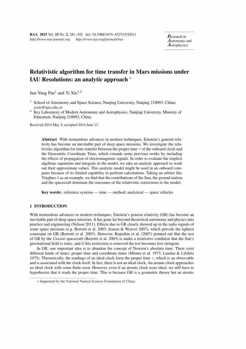
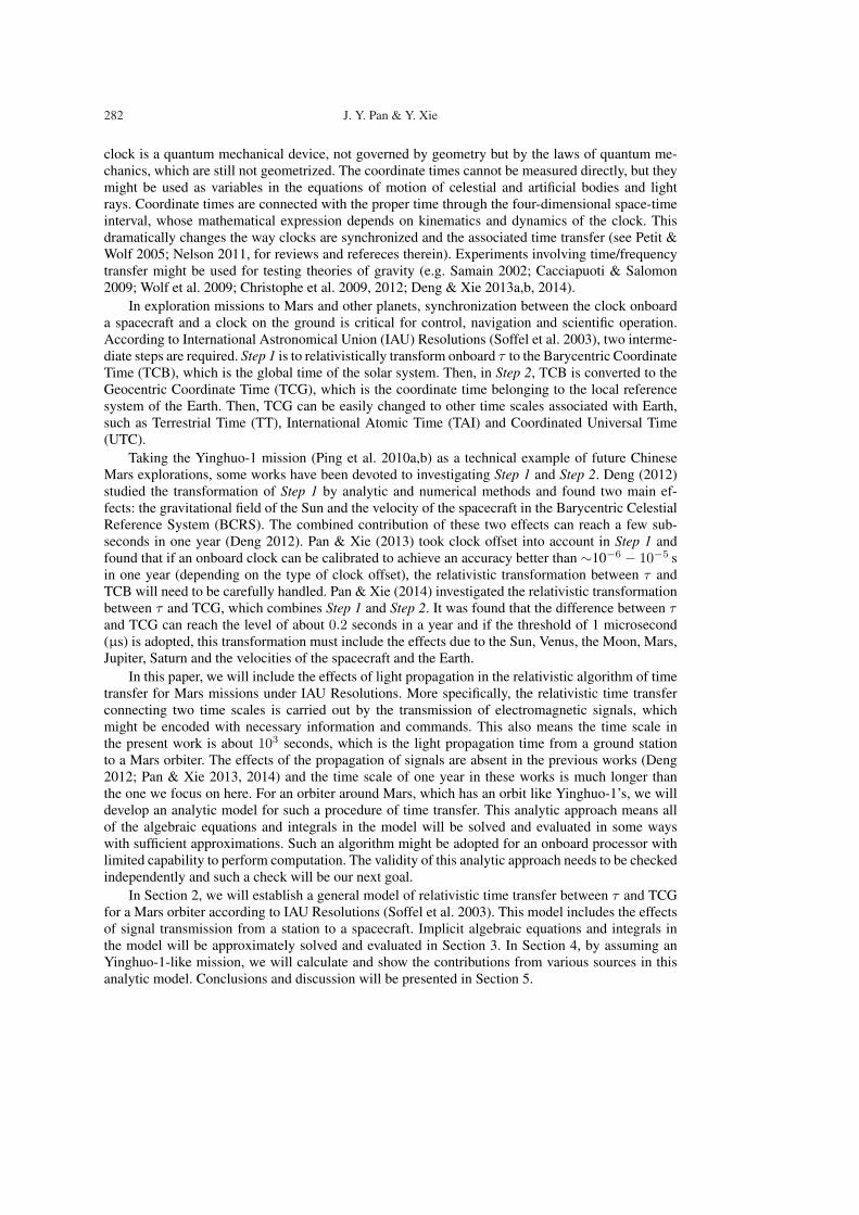
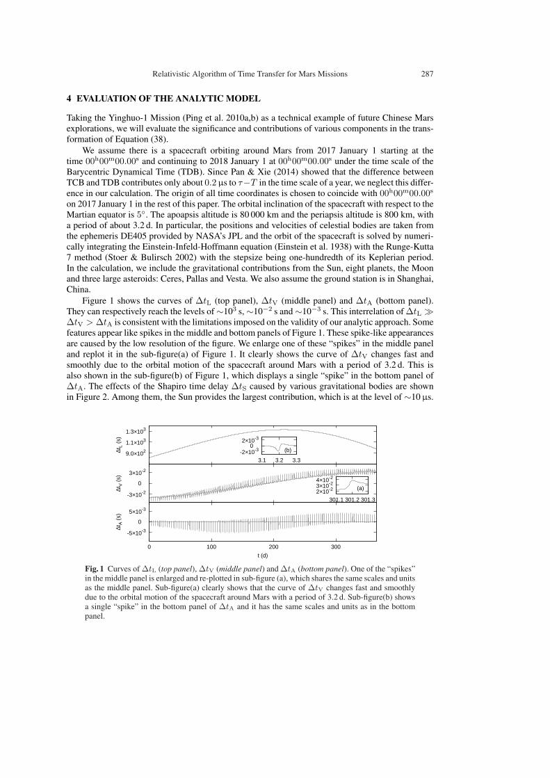
Figure 1 shows the curves of ∆tL (top panel), ∆tV (middle panel) and ∆tA (bottom panel).They can respectively reach the levels of∼103 s,∼10−2 s and∼10−3 s. This interrelation of ∆tL À∆tV > ∆tA is consistent with the limitations imposed on the validity of our analytic approach. Somefeatures appear like spikes in the middle and bottom panels of Figure 1. These spike-like appearancesare caused by the low resolution of the figure. We enlarge one of these “spikes” in the middle paneland replot it in the sub-figure(a) of Figure 1. It clearly shows the curve of ∆tV changes fast andsmoothly due to the orbital motion of the spacecraft around Mars with a period of 3.2 d. This isalso shown in the sub-figure(b) of Figure 1, which displays a single “spike” in the bottom panel of∆tA. The effects of the Shapiro time delay ∆tS caused by various gravitational bodies are shownin Figure 2. Among them, the Sun provides the largest contribution, which is at the level of ∼10 µs.

9.0×102

1.1×103

1.3×103

∆tL

(s)

-3×10-2

3×10-2

∆tV (

s)

0

-5×10-3

5×10-3

0 100 200 300

∆tA (

s)

t (d)

0

2×10-23×10-24×10-2

301.1 301.2 301.3

(a)

-2×10-3

2×10-3

3.1 3.2 3.3

0(b)

Fig. 1 Curves of ∆tL (top panel), ∆tV (middle panel) and ∆tA (bottom panel). One of the “spikes”in the middle panel is enlarged and re-plotted in sub-figure (a), which shares the same scales and unitsas the middle panel. Sub-figure(a) clearly shows that the curve of ∆tV changes fast and smoothlydue to the orbital motion of the spacecraft around Mars with a period of 3.2 d. Sub-figure(b) showsa single “spike” in the bottom panel of ∆tA and it has the same scales and units as in the bottompanel.


-5.0-4.5-4.0 Sun

-12-11-10 Mercury

-11-10-9 Venus

-9.8-9.5-9.2 Earth

-12.0-11.5-11.0 Moon

-10.8-10.5-10.2 Mars

-14.4-14.3-14.2

log 1

0(∆t

S ⋅

s-1)

Ceres

-15.0-14.7-14.4

log 1

0(∆t

S ⋅

s-1)

Vesta

-8.8-8.5-8.2 Jupiter

-9.3-9.2-9.1 Saturn

-10.7-10.4-10.1

0 100 200 300

t (d)

Uranus

-10.6-10.4-10.2

0 100 200 300

t (d)

Neptune

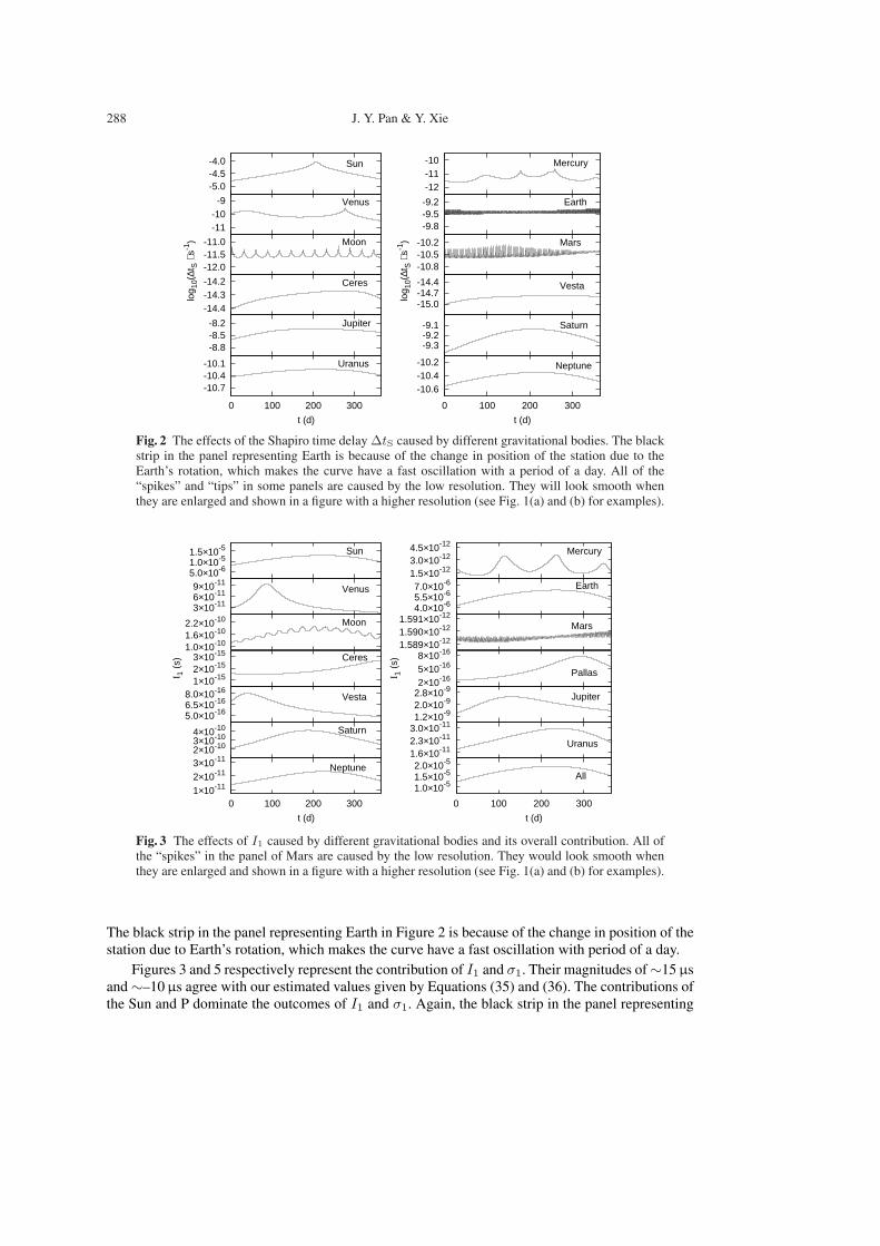
Fig. 2 The effects of the Shapiro time delay ∆tS caused by different gravitational bodies. The blackstrip in the panel representing Earth is because of the change in position of the station due to theEarth’s rotation, which makes the curve have a fast oscillation with a period of a day. All of the“spikes” and “tips” in some panels are caused by the low resolution. They will look smooth whenthey are enlarged and shown in a figure with a higher resolution (see Fig. 1(a) and (b) for examples).

5.0×10-61.0×10-51.5×10-5 Sun

1.5×10-123.0×10-124.5×10-12

Mercury

3×10-116×10-119×10-11

Venus

4.0×10-65.5×10-67.0×10-6 Earth

1.0×10-101.6×10-102.2×10-10 Moon

1.589×10-121.590×10-121.591×10-12

Mars

1×10-152×10-153×10-15

I 1 (

s) Ceres

2×10-165×10-168×10-16

I 1 (

s)

Pallas

5.0×10-166.5×10-168.0×10-16

Vesta

1.2×10-92.0×10-92.8×10-9

Jupiter

2×10-103×10-104×10-10 Saturn

1.6×10-112.3×10-113.0×10-11

Uranus

1×10-112×10-113×10-11

0 100 200 300

t (d)

Neptune

1.0×10-51.5×10-52.0×10-5

0 100 200 300

t (d)

All

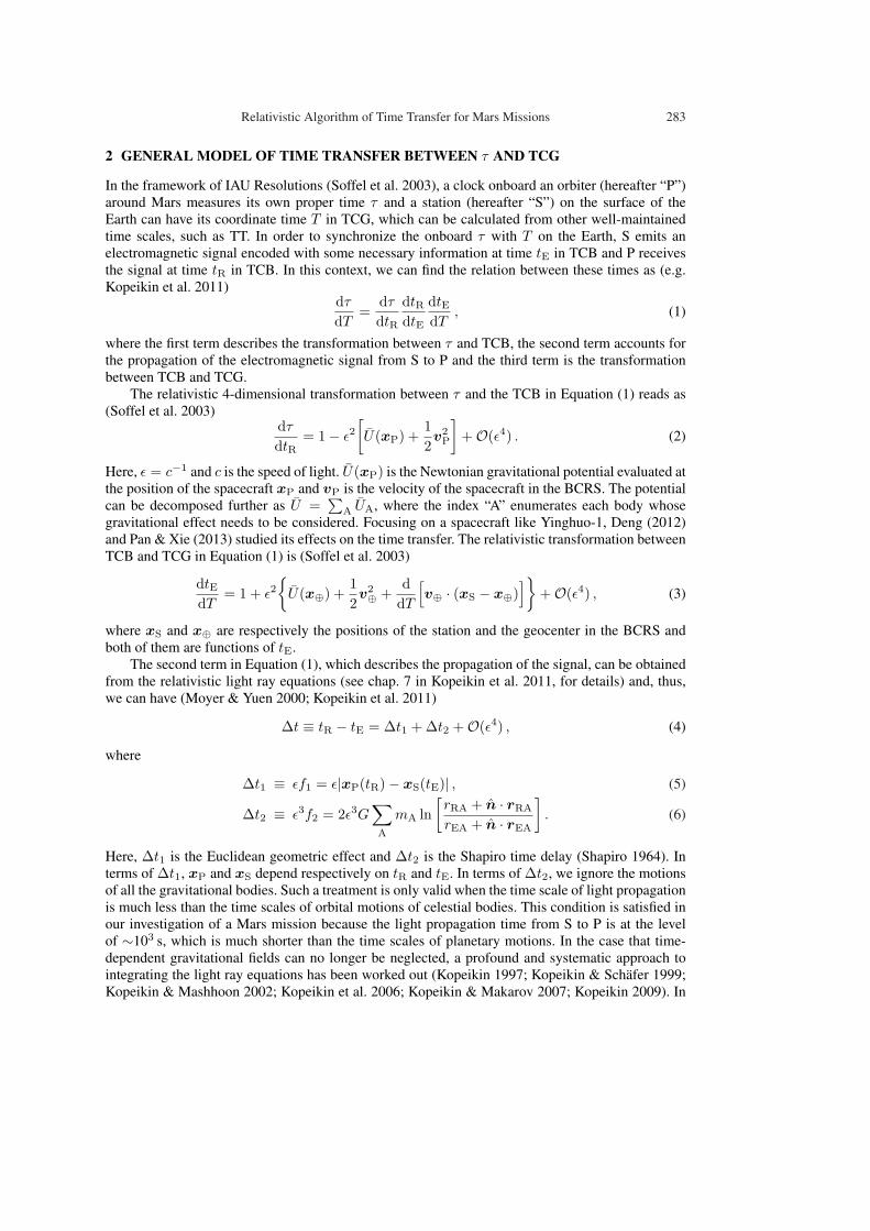
Fig. 3 The effects of I1 caused by different gravitational bodies and its overall contribution. All ofthe “spikes” in the panel of Mars are caused by the low resolution. They would look smooth whenthey are enlarged and shown in a figure with a higher resolution (see Fig. 1(a) and (b) for examples).

The black strip in the panel representing Earth in Figure 2 is because of the change in position of thestation due to Earth’s rotation, which makes the curve have a fast oscillation with period of a day.

Figures 3 and 5 respectively represent the contribution of I1 and σ1. Their magnitudes of∼15 µsand∼–10 µs agree with our estimated values given by Equations (35) and (36). The contributions ofthe Sun and P dominate the outcomes of I1 and σ1. Again, the black strip in the panel representing


-5×10-11

5×10-11 Sun0

-3×10-16

3×10-16 Mercury0

-1×10-14

1×10-14 Venus0

-5×10-11

5×10-11 Earth0

-1×10-11

1×10-11 Moon0

-5×10-17

5×10-17

Mars0

-1×10-19

1×10-19

I 2 (

s)

Ceres0

-3×10-20

3×10-20

I 2 (

s) Pallas0

-3×10-20

3×10-20

Vesta0

-5×10-14

5×10-14 Jupiter0

-5×10-15

5×10-15Saturn

0-2×10-16

2×10-16Uranus

0

-1×10-16

1×10-16

0 100 200 300

t (d)

Neptune0

-5×10-11

5×10-11

0 100 200 300

t (d)

All0

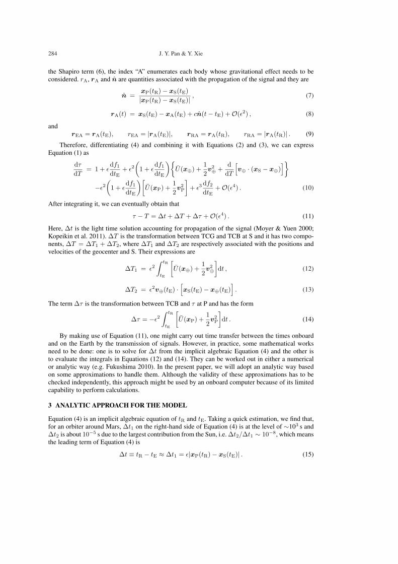
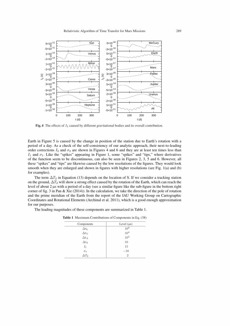
Fig. 4 The effects of I2 caused by different gravitational bodies and its overall contribution.

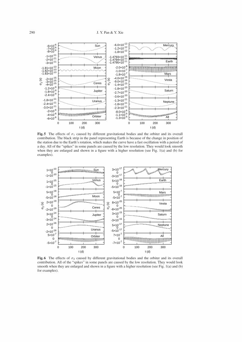
Earth in Figure 5 is caused by the change in position of the station due to Earth’s rotation with aperiod of a day. As a check of the self-consistency of our analytic approach, their next-to-leadingorder corrections I2 and σ2 are shown in Figures 4 and 6 and they are at least ten times less thanI1 and σ1. Like the “spikes” appearing in Figure 1, some “spikes” and “tips,” where derivativesof the function seem to be discontinuous, can also be seen in Figures 2, 3, 5 and 6. However, allthese “spikes” and “tips” are likewise caused by the low resolutions of the figures. They would looksmooth when they are enlarged and shown in figures with higher resolutions (see Fig. 1(a) and (b)for examples).

The term ∆T2 in Equation (13) depends on the location of S. If we consider a tracking stationon the ground, ∆T2 will show a strong effect caused by the rotation of the Earth, which can reach thelevel of about 2 µs with a period of a day (see a similar figure like the sub-figure in the bottom rightcorner of fig. 3 in Pan & Xie (2014)). In the calculation, we take the direction of the pole of rotationand the prime meridian of the Earth from the report of the IAU Working Group on CartographicCoordinates and Rotational Elements (Archinal et al. 2011), which is a good enough approximationfor our purposes.

The leading magnitudes of these components are summarized in Table 1.

Table 1 Maximum Contributions of Components in Eq. (38)

Components Level (µs)∆tL 109

∆tV 104

∆tA 103

∆tS 10

I1 15

σ1 −10

∆T2 2


-8×10-6-7×10-6-6×10-6 Sun

-1.8×10-12-1.2×10-12-6.0×10-13

Mercury

-3×10-11-2×10-11-1×10-11

Venus

-1.4795×10-11-1.4794×10-11-1.4793×10-11

Earth

-1.83×10-13-1.82×10-13-1.81×10-13 Moon

-1.8×10-7-1.0×10-7-2.0×10-8

Mars

-4×10-15-3×10-15-2×10-15

σ 1 (

s)

Ceres -1.4×10-15-9.0×10-16-4.0×10-16

σ 1 (

s) Vesta

-2.4×10-9-1.8×10-9-1.2×10-9

Jupiter

-3.6×10-10-2.7×10-10-1.8×10-10

Saturn

-3.0×10-11-2.4×10-11-1.8×10-11

Uranus

-2.3×10-11-1.8×10-11-1.3×10-11

Neptune

-6×10-6-4×10-6-2×10-6

0 100 200 300

t (d)

Orbiter -1.3×10-5-1.1×10-5-8.0×10-6

0 100 200 300

t (d)

All

Fig. 5 The effects of σ1 caused by different gravitational bodies and the orbiter and its overallcontribution. The black strip in the panel representing Earth is because of the change in position ofthe station due to the Earth’s rotation, which makes the curve have a fast oscillation with a period ofa day. All of the “spikes” in some panels are caused by the low resolution. They would look smoothwhen they are enlarged and shown in a figure with a higher resolution (see Fig. 1(a) and (b) forexamples).

-1×10-10

1×10-10 Sun0

-3×10-17

3×10-17 Mercury0

-1×10-15

1×10-15 Venus0

-5×10-16

5×10-16 Earth0

-5×10-18

5×10-18

Moon0-5×10-7

5×10-7Mars

0

-2×10-19

2×10-19

σ 2 (

s)

Ceres0

-8×10-20

8×10-20

σ 2 (

s) Vesta0

-3×10-14

3×10-14Jupiter

0-3×10-15

3×10-15Saturn

0

-2×10-16

2×10-16

Uranus0

-5×10-17

5×10-17 Neptune0

-5×10-7

5×10-7

0 100 200 300

t (d)

Orbiter0

-7×10-7

7×10-7

0 100 200 300

t (d)

All0

Fig. 6 The effects of σ2 caused by different gravitational bodies and the orbiter and its overallcontribution. All of the “spikes” in some panels are caused by the low resolution. They would looksmooth when they are enlarged and shown in a figure with a higher resolution (see Fig. 1(a) and (b)for examples).


5 CONCLUSIONS AND DISCUSSION

In this work, we take an Yinghuo-1-like mission as an example and investigate the relativistic al-gorithm for time transfer between the proper time τ of the onboard clock and TCG, which extendsprevious works (Deng 2012; Pan & Xie 2013, 2014) by including the effects of the propagation oflight signals. In order to evaluate the implicit algebraic equations and integrals in the model, we takean analytic approach to work out their approximate values. The analytic model (see Equation (38))might be used for an onboard computer because of its limited capability to perform calculations. Wefind that the contributions of the Sun, the ground station and the spacecraft dominate the outcomesof the relativistic corrections to the model.

Acknowledgements This work is funded by the National Natural Science Foundation of China(Grant Nos. 11103010 and J1210039), the Fundamental Research Program of Jiangsu Province ofChina (No. BK2011553) and the Research Fund for the Doctoral Program of Higher Education ofChina (No. 20110091120003).

References

Archinal, B. A., A’Hearn, M. F., Bowell, E., et al. 2011, Celestial Mechanics and Dynamical Astronomy,109, 101

Bertotti, B., Iess, L., & Tortora, P. 2003, Nature, 425, 374Cacciapuoti, L., & Salomon, C. 2009, European Physical Journal Special Topics, 172, 57Christophe, B., Andersen, P. H., Anderson, J. D., et al. 2009, Experimental Astronomy, 23, 529Christophe, B., Spilker, L. J., Anderson, J. D., et al. 2012, Experimental Astronomy, 34, 203Deng, X.-M. 2012, RAA (Research in Astronomy and Astrophysics), 12, 703Deng, X.-M., & Xie, Y. 2013a, RAA (Research in Astronomy and Astrophysics), 13, 1225Deng, X.-M., & Xie, Y. 2013b, MNRAS, 431, 3236Deng, X.-M., & Xie, Y. 2014, RAA (Research in Astronomy and Astrophysics), 14, 319Einstein, A., Infeld, L., & Hoffmann, B. 1938, Annals of Mathematics, 39, 65Fukushima, T. 2010, in IAU Symposium, 261, eds. S. A. Klioner, P. K. Seidelmann, & M. H. Soffel, 89Jensen, J. R., & Weaver, G. L. 2007, in Proc. 39th Annual Precise Time and Time Interval (PTTI) Meeting, 79Kopeikin, S., Efroimsky, M., & Kaplan, G. 2011, Relativistic Celestial Mechanics of the Solar System, eds.

S. Kopeikin, M. Efroimsky, & G. Kaplan (Wiley)Kopeikin, S., Korobkov, P., & Polnarev, A. 2006, Classical and Quantum Gravity, 23, 4299Kopeikin, S., & Mashhoon, B. 2002, Phys. Rev. D, 65, 064025Kopeikin, S. M. 1997, Journal of Mathematical Physics, 38, 2587Kopeikin, S. M. 2009, MNRAS, 399, 1539Kopeikin, S. M., & Makarov, V. V. 2007, Phys. Rev. D, 75, 062002Kopeikin, S. M., Polnarev, A. G., Schafer, G., & Vlasov, I. Y. 2007, Physics Letters A, 367, 276Kopeikin, S. M., & Schafer, G. 1999, Phys. Rev. D, 60, 124002Landau, L. D., & Lifshitz, E. M. 1975, The Classical Theory of Fields (4th edn.; Oxford: Pergamon Press)Misner, C. W., Thorne, K. S., & Wheeler, J. A. 1973, Gravitation (San Francisco: W. H. Freeman and Co.)Moyer, T. D., & Yuen, J. H. 2000, Formulation for Observed and Computed Values of Deep Space Network

Data Types for Navigation (Jet Propulsion Laboratory, National Aeronautics and Space Administration)Nelson, R. A. 2011, Metrologia, 48, 171Pan, J.-Y., & Xie, Y. 2013, RAA (Research in Astronomy and Astrophysics), 13, 1358Pan, J.-Y., & Xie, Y. 2014, RAA (Research in Astronomy and Astrophysics), 14, 233Petit, G., & Wolf, P. 2005, Metrologia, 42, 138Ping, J. S., Qian, Z. H., Hong, X. Y., et al. 2010a, in Lunar and Planetary Science Conference, 41, 1060


Ping, J.-S., Shang, K., Jian, N.-C., et al. 2010b, in Proceedings of the Ninth Asia-Pacific InternationalConference on Gravitation and Astrophysics, eds. J. Luo, Z.-B. Zhou, H.-C. Yeh, & J.-P. Hsu, 225

Samain, E. 2002, in EGS General Assembly Conference Abstracts, 27, 5808Shapiro, I. I. 1964, Physical Review Letters, 13, 789Soffel, M., Klioner, S. A., Petit, G., et al. 2003, AJ, 126, 2687Stoer, J., & Bulirsch, R. 2002, Introduction to Numerical Analysis (New York: Springer)Wolf, P., Borde, C. J., Clairon, A., et al. 2009, Experimental Astronomy, 23, 651

relativistic algorithm for time transfer in mars missions …€¦ · · 2015-01-15relativistic...

Documents