sycomore DocumentationRelease 1.3.1

Julien Lamy

Aug 16, 2021

Contents:

1 Installation 3

2 Usage 52.1 Installing Sycomore . . . . . . . . . . . . . . . . . . . . . . . . . . . . . . . . . . . . . . . . . . . 62.2 Common features . . . . . . . . . . . . . . . . . . . . . . . . . . . . . . . . . . . . . . . . . . . . . 82.3 Bloch simulation . . . . . . . . . . . . . . . . . . . . . . . . . . . . . . . . . . . . . . . . . . . . . 112.4 Extended Phase Graphs (EPG) . . . . . . . . . . . . . . . . . . . . . . . . . . . . . . . . . . . . . . 132.5 Configuration Model . . . . . . . . . . . . . . . . . . . . . . . . . . . . . . . . . . . . . . . . . . . 23

3 Indices and tables 25

Index 27

i

ii

sycomore Documentation, Release 1.3.1

matplotlib.pyplot.rcParams["font.size"] = 6

import pweavepweave.rcParams["chunk"]["defaultoptions"].update(

{"results": "hidden"})

Sycomore is an MRI simulation toolkit providing Bloch simulation, Extended Phase Graph (EPG) (both regularand discrete, including 3D), and Configuration Model. Sycomore is a Python packge in which all computationnaly-intensive operations are run by a C++ backend, providing a very fast runtime.

Sycomore is free software, released under the MIT license, and its source code is available on GitHub.

A sample web application, using Sycomore paired with Bokeh is available on Heroku: it presents classical MRIexperiments (RARE, RF-spoiling, slice profile with a selective sinc pulse), using the different simulation models ofSycomore.

Contents: 1

sycomore Documentation, Release 1.3.1

2 Contents:

CHAPTER 1

Installation

Packaged versions of Sycomore are available on pypi and Anaconda for Linux, macOS and Windows.

To install from Anaconda, type conda install -c conda-forge sycomore. To install from pypi, typepip3 install sycomore (or pip install sycomore). If you are installing from pypi and no pre-compiled version is available for your platform, pip will try to install from the source archive; in that case you willneed a C++11 compiler, CMake, xsimd and pybind11 to successfully build Sycomore.

Additional details, including building from source, are provided in the documentation.

As of May 2021, compatibility with Python 2 is still possible: however due to the end of life of Python 2, ensuringthis compatibility is not a goal of Sycomore, and no such package is distributed.

3

sycomore Documentation, Release 1.3.1

4 Chapter 1. Installation

CHAPTER 2

Usage

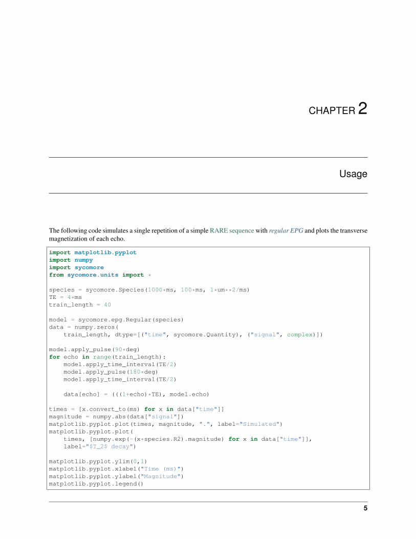
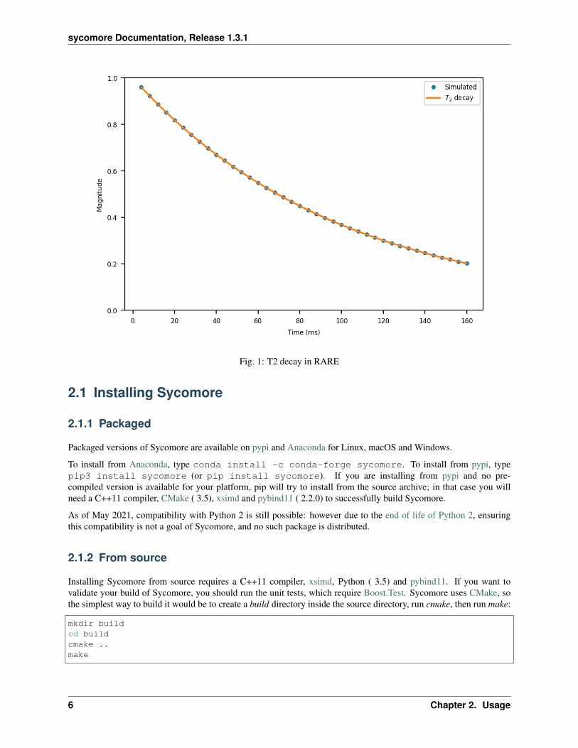
The following code simulates a single repetition of a simple RARE sequence with regular EPG and plots the transversemagnetization of each echo.

import matplotlib.pyplotimport numpyimport sycomorefrom sycomore.units import *

species = sycomore.Species(1000*ms, 100*ms, 1*um**2/ms)TE = 4*mstrain_length = 40

model = sycomore.epg.Regular(species)data = numpy.zeros(

train_length, dtype=[("time", sycomore.Quantity), ("signal", complex)])

model.apply_pulse(90*deg)for echo in range(train_length):

model.apply_time_interval(TE/2)model.apply_pulse(180*deg)model.apply_time_interval(TE/2)

data[echo] = (((1+echo)*TE), model.echo)

times = [x.convert_to(ms) for x in data["time"]]magnitude = numpy.abs(data["signal"])matplotlib.pyplot.plot(times, magnitude, ".", label="Simulated")matplotlib.pyplot.plot(

times, [numpy.exp(-(x*species.R2).magnitude) for x in data["time"]],label="$T_2$ decay")

matplotlib.pyplot.ylim(0,1)matplotlib.pyplot.xlabel("Time (ms)")matplotlib.pyplot.ylabel("Magnitude")matplotlib.pyplot.legend()

5

sycomore Documentation, Release 1.3.1

Fig. 1: T2 decay in RARE

2.1 Installing Sycomore

2.1.1 Packaged

Packaged versions of Sycomore are available on pypi and Anaconda for Linux, macOS and Windows.

To install from Anaconda, type conda install -c conda-forge sycomore. To install from pypi, typepip3 install sycomore (or pip install sycomore). If you are installing from pypi and no pre-compiled version is available for your platform, pip will try to install from the source archive; in that case you willneed a C++11 compiler, CMake ( 3.5), xsimd and pybind11 ( 2.2.0) to successfully build Sycomore.

As of May 2021, compatibility with Python 2 is still possible: however due to the end of life of Python 2, ensuringthis compatibility is not a goal of Sycomore, and no such package is distributed.

2.1.2 From source

Installing Sycomore from source requires a C++11 compiler, xsimd, Python ( 3.5) and pybind11. If you want tovalidate your build of Sycomore, you should run the unit tests, which require Boost.Test. Sycomore uses CMake, sothe simplest way to build it would be to create a build directory inside the source directory, run cmake, then run make:

mkdir buildcd buildcmake ..make

6 Chapter 2. Usage

sycomore Documentation, Release 1.3.1

In addition to the common CMake options (e.g. CMAKE_BUILD_TYPE or CMAKE_INSTALL_PREFIX), Sycomoremay be built with the following options:

• BUILD_SHARED_LIBS controls the generation of static libraries or share libraries; defaults to ON, i.e. buildingshared libraries

• BUILD_TESTING controls the build of the C++ unit test executables; defaults to ON, i.e. the unit tests arecompiled

• BUILD_PYTHON_WRAPPERS controls the build of the Python wrappers; defaults to ON, i.e. the Pythonwrappers are built

• BUILD_STANDALONE_PYTHON_WRAPPERS, controls whether a standalone Python library is built, wihtoutany pure C++ compatibility; defaults to OFF, i.e. both the C++ and Python libraries are built

The compilation can take advantage of a multi-core CPU either by using make with the -jN flag (where N is the numberof concurrent tasks, i.e. the number of cores) or by using Ninja. Once the compilation succeeds, the units tests can berun from the build directory:

export SYCOMORE_TEST_DATA=$(pwd)/../tests/datactest -T Testpython3 -m unittest discover -s ../tests/python/

This code benefits hugely from compiler optimizations. It is recommended to build a Release version and use extracompiler flags to speed-up the simulations. Details of these flags on Linux and macOS are provided in the nextsections.

Debian and Ubuntu

The following call to apt-get will install most dependencies:

apt-get install -y cmake g++ libboost-dev libboost-test-dev libpython3-dev python3-→˓distutils python3-pybind11

As of Debian 10 (Buster) and Ubuntu 21.04 (Hirsute Hippo), xsimd is not available as a package. Its installation ishowever easy: after fetching and unzipping the latest release, run the following commands from within the sourcedirectory:

cmake -DCMAKE_INSTALL_PREFIX=~/local .cmake --build . --target install

When compiling with GCC on Debian or Ubuntu, -ffast-math enables -ffinite-math-only, which breaks some partsof the Configuration Model implementation in Sycomore (the application of a time interval with gradients or thecomputation of isochromat with off-resonance effects). All other optimizations turned on by -ffast-math can howeverbe used and the recommended call to CMake is:

cmake \-DCMAKE_BUILD_TYPE=Release \-DCMAKE_CXX_FLAGS="-march=native -fno-math-errno -funsafe-math-optimizations -fno-

→˓rounding-math -fno-signaling-nans -fcx-limited-range -fexcess-precision=fast -D__→˓FAST_MATH__" \-DPYTHON_EXECUTABLE=/usr/bin/python3 \..

For more details on floating point math with GCC, refer to the official documentation.

2.1. Installing Sycomore 7

sycomore Documentation, Release 1.3.1

macOS with Homebrew

The following call to brew will install all dependencies:

brew install boost cmake pybind11 xsimd

The documentation of the -ffast-math option in Clang is rather terse, but the source code provides more details. Despitedisabling non-finite maths, using -ffast-math does not break Sycomore. The recommended call to CMake is:

cmake \-DCMAKE_BUILD_TYPE=Release \-DCMAKE_CXX_FLAGS="-march=native -ffast-math" \../

2.2 Common features

2.2.1 Units

MRI simulations deal with various quantities: times, frequencies and angular frequencies, magnetic field strength,gradient moments, etc. All those quantities use different usual prefixes, but not always the same: relaxation timeand sequence timing are usually expressed in milliseconds, while the gyromagnetic ratio is expressed in MHz/T (i.e.inverse of microseconds) gradients moments are expressed in mT/mms and slice thickness in millimeters (on clinicalscanners) or micrometers (on pre-clinical scanners). This wealth of units makes it very easy to get quantities wrongby a factor of 1000 or more.

Sycomore provides a unit system so that users do not have to convert their quantities to a specific unit. Units may bedeclared by multiplying or dividing by the unit name (e.g. 500*ms). Those two syntaxes can be mixed in order touse more complex units (e.g. 267.522*MHz/T). Unit objects follow the usual arithmetic rules, and all SI base units,derived units and prefixes are defined.

sycomore.Quantity objects contain their value in the base SI unit and may be converted to a compatible unit.Common arithmetic operations (addition, subtraction, multiplication, division, power) are implemented, as well asmost of numpy numeric functions. The following code sample summarizes these features.

Note: The micro prefix is u, not 𝜇, in order to keep ASCII names

import sycomorefrom sycomore.units import *

# Combination of base unitsdiffusion_coefficient = 0.89*um**2/ms

# Magnitude of the quantity, in SI unitlength = 180*cmlength_in_meters = length.magnitude # Equals to 1.8

# Conversion: magnitude of the quantity, in specified unitduration = 1*hduration_in_seconds = duration.convert_to(s) # Equals to 3600

Note: Take caution when importing all units name (from sycomore.units import *), as some names mayclash with your code. In a long module with many variables, it is better to import only the required units (e.g. from

8 Chapter 2. Usage

sycomore Documentation, Release 1.3.1

sycomore.units import mT, m, ms)

2.2.2 Species

A species is characterized by its relaxation rates (R1, R2 and R2’), its diffusivity D and its relative resonance fre-

quency ∆𝜔. It is described by the sycomore.Species class. R1 and R2 are mandatory parameters, all others areoptional and are equal to 0 if unspecified. Using the unit system, relaxation rates and relaxation times may be usedinterchangeably.

import sycomorefrom sycomore.units import *

# Create a Species from either relaxation times, relaxation rates or bothspecies = sycomore.Species(1000*ms, 100*ms)species = sycomore.Species(1*Hz, 10*Hz)species = sycomore.Species(1000*ms, 10*Hz)

The diffusivity can be assigned either as a scalar (for isotropic diffusion) or as a tensor (for anistropic diffusion), butwill always be returned as a tensor:

import sycomorefrom sycomore.units import *

species = sycomore.Species(1000*ms, 100*ms)# Assign the diffusion coefficient as a scalarspecies.D = 3*um**2/s# The diffusion coefficient is stored on the diagonal of the tensorprint(species.D[0])

# Assign the diffusion coefficient as a tensorspecies.D = [

3*um**2/s, 0*um**2/s, 0*um**2/s,0*um**2/s, 2*um**2/s, 0*um**2/s,0*um**2/s, 0*um**2/s, 1*um**2/s]

print(species.D)

3e-12 [ L^2 T^-1 ](3e-12 [ L^2 T^-1 ] 0 [ L^2 T^-1 ] 0 [ L^2 T^-1 ] 0 [ L^2 T^-1 ] 2e-12[ L^2 T^-1 ] 0 [ L^2 T^-1 ] 0 [ L^2 T^-1 ] 0 [ L^2 T^-1 ] 1e-12 [ L^2T^-1 ])

2.2.3 Time intervals

A time interval is specified by its duration and an optional magnetic field gradient. The gradient can be either as ascalar or as a 3D array, and can describe the amplitude (in T/m), the area (in T/m*s) or the dephasing (in rad/m). Asycomore.TimeInterval.set_gradient() function is available for generic modification of the gradient.

import sycomorefrom sycomore.units import *

# Scalar gradient, defined by its amplitudeinterval = sycomore.TimeInterval(1*ms, 20*mT/m)print(

(continues on next page)

2.2. Common features 9

sycomore Documentation, Release 1.3.1

(continued from previous page)

interval.duration, "\n",interval.gradient_amplitude, "\n",interval.gradient_area/interval.duration, "\n",interval.gradient_dephasing/(sycomore.gamma*interval.duration))

0.001 [ T ](0.02 [ L^-1 M T^-2 I^-1 ] 0.02 [ L^-1 M T^-2 I^-1 ] 0.02 [ L^-1 M

T^-2 I^-1 ])(0.02 [ L^-1 M T^-2 I^-1 ] 0.02 [ L^-1 M T^-2 I^-1 ] 0.02 [ L^-1 M

T^-2 I^-1 ])(0.02 [ L^-1 M T^-2 I^-1 ] 0.02 [ L^-1 M T^-2 I^-1 ] 0.02 [ L^-1 M

T^-2 I^-1 ])

2.2.4 Reference

class sycomore.Quantity

magnitudeThe magnitude of the quantity, in SI units.

convert_to(unit)Return the scalar value of the quantity converted to the given unit.

class sycomore.Species(R1, R2, D=0*m**2/s, R2_prime=0*Hz, delta_omega=0*rad/s)

R1Longitudinal relaxation rate

T1Longitudinal relaxation time

R2Transversal relaxation rate

T2Transversal relaxation time

DDiffusion tensor

R2_primeThe part of the apparent transversal relaxation rate R2

* attributed to the magnetic field inhomogeneity

T2_primeThe part of the apparent transversal relaxation time T2

* attributed to the magnetic field inhomogeneity

delta_omegaFrequency offset

class sycomore.TimeInterval(duration, gradient=0*T/m)Gradient may be specified as amplitude (in T/m), area (in T/m*s) or dephasing (in rad/m).

durationDuration of the time interval

gradient_amplitudeAmplitude of the gradient

10 Chapter 2. Usage

sycomore Documentation, Release 1.3.1

gradient_areaArea of the gradient (duration×amplitude)

gradient_dephasingDephasing caused by the gradient (𝛾×duration×amplitude)

gradient_momentAlias for dephasing

set_gradient()Set the gradient of the time interval, either as amplitude, area or dephasing

2.3 Bloch simulation

The Bloch simulation (or isochromat simulation) in Sycomore is based on Hargreaves’s 2001 paper Characterizationand Reduction of the Transient Response in Steady-State MR Imaging where limiting cases of the full spin behavior(instantaneous RF pulse, “pure” relaxation, “pure” precession, etc.) are expressed as matrices. The matrices repre-senting building blocks of a sequence are multiplied amongst them, forming a single matrix operator for a repetition.Iterating this process yields a fast simulation of the evolution of a single isochromat and the eigenanalysis of theresulting matrix yields important insights on the steady-state of the sequence.

2.3.1 Homogeneous coordinates

An homogeneous form of all matrices and vectors is used to obtain a purely multiplicative form of the matrix oper-ators. Using homogenous coordinates (also called projective coordinates), a vector in R3 with Cartesian coordinates(𝑥𝑐, 𝑦𝑐, 𝑧𝑐) is represented as a set of 4D vectors in PR3, the three-dimensional projective space, (𝑥𝑝, 𝑦𝑝, 𝑧𝑝, 𝑤) so that(𝑥𝑐, 𝑦𝑐, 𝑧𝑐) = (𝑥𝑝/𝑤, 𝑦𝑝/𝑤, 𝑧𝑝/𝑤). In this representation, any geometric transformation which can be expressed as a3×3 matrix 𝑀 can also be represented as a 4×4 homogeneous matrix:⎡⎢⎢⎣ 𝑀

000

0 0 0 1

⎤⎥⎥⎦Moreover, a translation T = (𝑇𝑥, 𝑇𝑦, 𝑇𝑧) can also be represented as a 4×4 homogeneous matrix:⎡⎢⎢⎣

1 0 0 𝑇𝑥

0 1 0 𝑇𝑦

0 0 1 𝑇𝑧

0 0 0 1

⎤⎥⎥⎦The composition of the geometric transforms described by those homogeneous matrices is given by multiplying thematrices, as is the case in Euclidean coordinates.

2.3.2 Usage

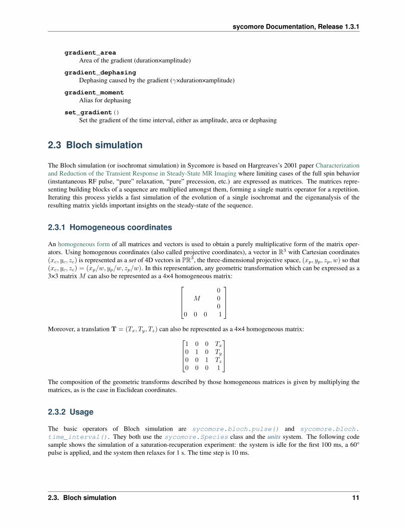
The basic operators of Bloch simulation are sycomore.bloch.pulse() and sycomore.bloch.time_interval(). They both use the sycomore.Species class and the units system. The following codesample shows the simulation of a saturation-recuperation experiment: the system is idle for the first 100 ms, a 60°pulse is applied, and the system then relaxes for 1 s. The time step is 10 ms.

2.3. Bloch simulation 11

sycomore Documentation, Release 1.3.1

import matplotlib.pyplotimport numpyimport sycomorefrom sycomore.units import *

species = sycomore.Species(1000*ms, 100*ms)flip_angle = 60*deg

idle = sycomore.bloch.time_interval(species, 10*ms)pulse = sycomore.bloch.pulse(flip_angle)

t = 0*sM = numpy.array([0,0,1,1])

record = [[t, M[:3]/M[3]]]for _ in range(10):

t = t+10*msM = idle @ Mrecord.append([t, M[:3]/M[3]])

M = pulse @ Mrecord.append([t, M[:3]/M[3]])

for _ in range(100):t = t+10*msM = idle @ Mrecord.append([t, M[:3]/M[3]])

time, magnetization = list(zip(*record))magnetization = numpy.array(magnetization)

x_axis = [x.convert_to(ms) for x in time]matplotlib.pyplot.plot(

x_axis, numpy.linalg.norm(magnetization[:, :2], axis=-1), label="$M_\perp$")matplotlib.pyplot.plot(x_axis, magnetization[:, 2], label="$M_z$")matplotlib.pyplot.xlim(0)matplotlib.pyplot.ylim(-0.02)matplotlib.pyplot.xlabel("Time (ms)")matplotlib.pyplot.ylabel("$M/M_0$")matplotlib.pyplot.legend()matplotlib.pyplot.tight_layout()

2.3.3 Reference

sycomore.bloch.pulse(angle, phase=0*rad)Instantaneous RF pulse with specified angle and phase.

sycomore.bloch.time_interval(species, duration, delta_omega=0*Hz, gradient_amplitude=0*T/m,position=0*m)

Composition of relaxation and phase accumulation.

sycomore.bloch.relaxation(species, duration)“Pure” relaxation process.

sycomore.bloch.phase_accumulation(angle)“Pure” precession.

12 Chapter 2. Usage

sycomore Documentation, Release 1.3.1

Fig. 2: Saturation-recuperation using Bloch simulation

2.4 Extended Phase Graphs (EPG)

Extended Phase Graphs (EPG) are first described in Hennig’s 1988 paper Multiecho imaging sequences with lowrefocusing flip angles – although the term “Extended Phase Graph” appears in a later paper (Echoes—how to generate,recognize, use or avoid them) – is an invaluable tool for fast simulation of MRI sequences. It allows simulation of allmain phenomena, including diffusion, motion, and magnetization transfer.

The EPG model is based on the spatial Fourier transform of the isochromats present in a voxel. Originally developpedfor sequences with a very regular time course (e.g. RARE or bSSFP), it has been later extended for non-regularsequences

Sycomore provides three EPG models:

• a one-dimensional regular model where all gradient moments throughout the simulation are assumed equal,

• a one-dimensional discrete model where gradients moments may differ, their values being discretized (i.e.binned) to avoid numerical instabilities along the simulation,

• a three-dimensional discrete model, where gradients can be specified in three dimensions.

2.4.1 Regular (constant gradient moment) EPG

In the regular EPG model, the dephasing order is reduced to a unitless integer 𝑘 ≥ 0 which represents a mul-tiplicative factor of some arbitrary basic dephasing. The implementation of regular EPG in Sycomore has twohigh-level operations: sycomore.Regular.apply_pulse() to simulate an RF hard pulse and sycomore.Regular.apply_time_interval() which simulates relaxation, diffusion and dephasing due to gradients. Thelower-level EPG operators used by sycomore.Regular.apply_time_interval() are also accessible as

2.4. Extended Phase Graphs (EPG) 13

sycomore Documentation, Release 1.3.1

sycomore.Regular.relaxation(), sycomore.Regular.diffusion() and sycomore.Regular.shift(). The states of the model are stored in sycomore.Regular.states, and the fully-focused magnetiza-tion (i.e. 𝐹0) is stored in sycomore.Regular.echo.

For simulations involving multiple gradient moments (all multiple of a given gradient moment), the “unit” gradientmoment must be declared when creating the model; for simulations involving only a single gradient moment, thisdeclaration is optional, but should be present nevertheless.

The following code sample simulates the evolution of the signal in an RF- & gradient spoiled GRE experiment.

import matplotlib.pyplotimport numpyimport sycomorefrom sycomore.units import *

species = sycomore.Species(1000*ms, 1000*ms)flip_angle=30*degTE = 5*msTR = 25*msphase_step = 117*degslice_thickness = 1*mmG_readout = 2*numpy.pi*rad / (sycomore.gamma*slice_thickness)

model = sycomore.epg.Regular(species, unit_gradient_area=G_readout)repetitions = int((4*species.T1/TR))

echo = numpy.zeros(repetitions, dtype=complex)for r in range(0, repetitions):

phase = (phase_step * 1/2*(r+1)*r)

model.apply_pulse(flip_angle, phase)model.apply_time_interval(TE)

rewind = numpy.exp(-1j*phase.convert_to(rad))echo[r] = model.echo*rewind

model.apply_time_interval(TR-TE, G_readout/(TR-TE))

Once the echo signal has been gathered for all repetitions, its magnitude and phase can be plotted using respectivelynumpy.abs and numpy.angle.

Reference

class sycomore.epg.Regular(species, initial_magnetization=Magnetization(0, 0,1), initial_size=100, unit_gradient_area=0*mT/m*ms,gradient_tolerance=1e-5)

speciesThe species being simulated

thresholdMinimum population of a state below which the state is considered emtpy (defaults to 0).

delta_omegaFreqency offset (defaults to 0 Hz).

velocityVelocity of coherent motion (defaults to 0 m/s).

14 Chapter 2. Usage

sycomore Documentation, Release 1.3.1

Fig. 3: Simulation of RF spoiling with regular EPG, using different phase steps

2.4. Extended Phase Graphs (EPG) 15

sycomore Documentation, Release 1.3.1

unit_gradient_areaUnit gradient area of the model.

states_countThe number of states currently stored by the model. This attribute is read-only.

statesThe sequence of states currently stored by the model. This attribute is a read-only, 3×N array of complexnumbers.

echoThe echo signal, i.e. 𝐹0 (read-only).

state(index)Return the magnetization at a given state, expressed by its index.

apply_pulse(angle, phase=0*rad)Apply an RF hard pulse.

apply_time_interval(duration, gradient=0*T/m)Apply a time interval, i.e. relaxation, diffusion, and gradient.

apply_time_interval(time_interval)Apply a time interval, i.e. relaxation, diffusion, and gradient.

shift()Apply a unit gradient; in regular EPG, this shifts all orders by 1.

shift(duration, gradient)Apply an arbitrary gradient; in regular EPG, this shifts all orders by an integer number corresponding to amultiple of the unit gradient.

relaxation(duration, gradient)Simulate the relaxation during given duration.

diffusion(duration, gradient)Simulate diffusion during given duration with given gradient amplitude.

off_resonance(duration)Simulate field- and species related off-resonance effects during given duration with given frequency offset.

2.4.2 Discrete (arbitrary gradient moment) EPG

In the discrete EPG model, the gradient moments may vary across time intervals. In this model, the orders of the modelare stored in bins of user-specified width (hence the term “discrete”), expressed in rad/m. The interface is similar tothat of regular EPG.

The following code sample show the full simulation of the DW-DESS sequence, with its two read-out modules andits diffusion module. Since the read-out gradient moment is largely smaller than the diffusion gradient moment,its simulation using regular EPG would require to subdivide every time interval to a common duration: with theparameters of the following simulation, even if we neglect the pre-phasing, each repetition would generate over 20new states with regular EPG, while at most 12 will be generated with discrete EPG.

import numpyimport sycomorefrom sycomore.units import *

species = sycomore.Species(1000*ms, 100*ms, 1*um**2/ms)flip_angle=20*deg

(continues on next page)

16 Chapter 2. Usage

sycomore Documentation, Release 1.3.1

(continued from previous page)

# Timingsprephasing = 1*usTE = 1*msTR = 10*mstau = TR - 2*TE - 2*prephasing # Duration of diffusion gradient# Gradientsslice_thickness = 1*mmG_readout = 2*numpy.pi*rad / (sycomore.gamma*slice_thickness)G_diffusion = 200*mT/m*ms

model = sycomore.epg.Discrete(species)repetitions = int((4*species.T1/TR))

FID = numpy.zeros(repetitions, dtype=complex)echo = numpy.zeros(repetitions, dtype=complex)for repetition in range(repetitions):

model.apply_pulse(flip_angle)

model.apply_time_interval(prephasing, -G_readout/2/prephasing)model.apply_time_interval(TE/2, G_readout/2/(TE/2))FID[repetition] = model.echomodel.apply_time_interval(TE/2, G_readout/2/(TE/2))

model.apply_time_interval(tau, G_diffusion/tau)

model.apply_time_interval(TE/2, G_readout/2/(TE/2))echo[repetition] = model.echomodel.apply_time_interval(TE/2, G_readout/2/(TE/2))model.apply_time_interval(prephasing, -G_readout/2/prephasing)

Note: The default bin width of 𝛿𝑘 = 1 rad/m corresponds to a gradient area of 𝛿𝑘/𝛾 ≈ 3 𝜇T/m ms. The dephasingorders are stored as 64-bits, signed integers; the default bin width hence allows to handle dephasing orders in the range[︀−9 · 1018 rad/m,+9 · 1018 rad/m

]︀, i.e.

[︀−3 · 1016 mT/m ms,+3 · 1016 mT/m ms

]︀The previous code will generate a large number of states, which will translate to a long execution time. Better per-formance can be gained by discarding the states with a low population, at the expense of a slight losss in preci-sion: this is achieved by passing a non-zero value to the threshold parameter of the sycomore.epg.Discrete.apply_time_interval() function. As an example, using a threshold of 10−4 in the previous simulation dras-tically reduces the computation time from 5 minutes to 50 ms while conserving a good precision, as shown in thefollowing figure.

Reference

class sycomore.epg.Discrete(species, initial_magnetization=Magnetization(0, 0, 1),bin_width=1*rad/m)

speciesThe species being simulated

thresholdMinimum population of a state below which the state is considered emtpy (defaults to 0).

delta_omegaFreqency offset (defaults to 0 Hz).

2.4. Extended Phase Graphs (EPG) 17

sycomore Documentation, Release 1.3.1

Fig. 4: Simulation of DW-DESS with discrete EPG, without threshold (plain lines) and with threshold (dots)

18 Chapter 2. Usage

sycomore Documentation, Release 1.3.1

ordersThe sequence of orders currently stored by the model, in the same order as the states member. Thisattribute is read-only.

statesThe sequence of states currently stored by the model, in the same order as the orders member. Thisattribute is a read-only, 3×N array of complex numbers.

echoThe echo signal, i.e. 𝐹0 (read-only).

bin_widthDiscretization of orders, in rad/m (read-only).

state(index)Return the magnetization at a given state, expressed by its index.

state(order)Return the magnetization at a given state, expressed by its order.

apply_pulse(angle, phase=0*rad)Apply an RF hard pulse.

apply_time_interval(duration, gradient=0*T/m, threshold=0.)Apply a time interval, i.e. relaxation, diffusion, and gradient. States with a population lower than thresholdwill be removed.

apply_time_interval(time_interval)Apply a time interval, i.e. relaxation, diffusion, and gradient.

shift(duration, gradient)Apply a gradient; in discrete EPG, this shifts all orders by specified value.

relaxation(duration, gradient)Simulate the relaxation during given duration.

diffusion(duration, gradient)Simulate diffusion during given duration with given gradient amplitude.

off_resonance(duration)Simulate field- and species related off-resonance effects during given duration with given frequency offset.

2.4.3 Discrete (arbitrary gradient moment) EPG in 3D

In the 3D discrete EPG model, the gradient moments may vary across time intervals as in regular EPG, but theiramplitude is specified on the three spatial axes.

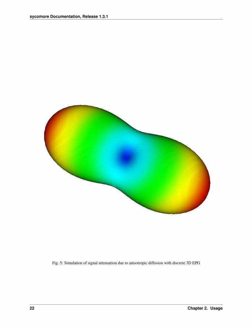
The following code sample simulates a PGSE diffusion sequence in an anisotropic medium and shows the dependencyof the signal attenuation to the relative orientation of diffusion tensor and of the diffusion gradient.

import numpyimport sycomorefrom sycomore.units import *import vtkimport vtk.numpy_interface.dataset_adapter

species = sycomore.Species(1000*ms, 100*ms, numpy.diag([4000, 1500, 10])*um**2/s)

TE = 50*ms

(continues on next page)

2.4. Extended Phase Graphs (EPG) 19

sycomore Documentation, Release 1.3.1

(continued from previous page)

G = 50*mT/mdelta = 18*ms# Since b = (𝛾G𝛿)^2 (Δ-𝛿/3) and Δ = TE-𝛿, the b-value is:print(

"b={:.0f} s/mm2".format(((sycomore.gamma*G*delta)**2 * (TE-4/3*delta)).convert_to(s/mm**2)))

def dw_se(species, TE, G, delta):model = sycomore.epg.Discrete3D(species)

# Excitationmodel.apply_pulse(90*deg)

# Diffusion-sensitization gradient and mixing timemodel.apply_time_interval(delta, G)model.apply_time_interval(TE/2-delta)

# Refocussingmodel.apply_pulse(180*deg)

# Mixing time and diffusion-sensitization gradientmodel.apply_time_interval(TE/2-delta)model.apply_time_interval(delta, G)

return numpy.abs(model.echo)

# Generate a unit spheresphere_source = vtk.vtkSphereSource()sphere_source.SetRadius(1)sphere_source.SetThetaResolution(50)sphere_source.SetPhiResolution(50)sphere_source.Update()sphere = vtk.numpy_interface.dataset_adapter.WrapDataObject(

sphere_source.GetOutput())print(len(sphere.Points), "points on sphere")

# Simulate the sequence with a diffusion gradient along each point on the sphereS_0 = dw_se(species, TE, [0*mT/m, 0*mT/m, 0*mT/m], delta)attenuation = numpy.zeros((len(sphere.Points)))for index, direction in enumerate(sphere.Points):

S = dw_se(species, TE, direction*G, delta)attenuation[index] = S/S_0sphere.Points[index] *= attenuation[index]

sphere.PointData.append(1-attenuation, "Attenuation")sphere.PointData.SetActiveScalars("Attenuation")

# Recompute the normals of the surfacenormals = vtk.vtkPolyDataNormals()normals.SetInputData(sphere.VTKObject)

# Plot the resultmapper = vtk.vtkPolyDataMapper()mapper.SetInputConnection(normals.GetOutputPort())actor = vtk.vtkActor()actor.SetMapper(mapper)

renderer = vtk.vtkRenderer()(continues on next page)

20 Chapter 2. Usage

sycomore Documentation, Release 1.3.1

(continued from previous page)

renderer.AddActor(actor)renderer.SetBackground(1, 1, 1)renderer.GetActiveCamera().SetPosition(4, -0.7, -0.3)renderer.GetActiveCamera().SetViewUp(0.2, 0.9, 0.4)

window = vtk.vtkRenderWindow()window.AddRenderer(renderer)window.SetSize(800, 800)window.SetOffScreenRendering(True)

to_image = vtk.vtkWindowToImageFilter()to_image.SetInput(window)png_writer = vtk.vtkPNGWriter()png_writer.SetInputConnection(to_image.GetOutputPort())png_writer.SetFileName("anisotropic_diffusion.png")png_writer.Write()

b=1507 s/mm2

2402 points on sphere

Reference

class sycomore.epg.Discrete3D(species, initial_magnetization=Magnetization(0, 0, 1),bin_width=1*rad/m)

speciesThe species being simulated

thresholdMinimum population of a state below which the state is considered emtpy (defaults to 0).

delta_omegaFreqency offset (defaults to 0 Hz).

ordersThe sequence of orders currently stored by the model, in the same order as the states member. Thisattribute is read-only, Nx3 array of dephasing (in rad/m).

statesThe sequence of states currently stored by the model, in the same order as the orders member. Thisattribute is a read-only array of complex numbers (F(k), Z(k)).

echoThe echo signal, i.e. 𝐹0 (read-only).

bin_widthDiscretization of orders, in rad/m (read-only).

state(index)Return the magnetization at a given state, expressed by its index.

state(order)Return the magnetization at a given state, expressed by its order.

apply_pulse(angle, phase=0*rad)Apply an RF hard pulse.

2.4. Extended Phase Graphs (EPG) 21

sycomore Documentation, Release 1.3.1

Fig. 5: Simulation of signal attenuation due to anisotropic diffusion with discrete 3D EPG

22 Chapter 2. Usage

sycomore Documentation, Release 1.3.1

apply_time_interval(duration, gradient=[0*T/m, 0*T/m, 0*T/m], threshold=0.)Apply a time interval, i.e. relaxation, diffusion, and gradient. States with a population lower than thresholdwill be removed.

apply_time_interval(time_interval)Apply a time interval, i.e. relaxation, diffusion, and gradient.

shift(duration, gradient)Apply a gradient; in discrete EPG, this shifts all orders by specified value.

relaxation(duration, gradient)Simulate the relaxation during given duration.

diffusion(duration, gradient)Simulate diffusion during given duration with given gradient amplitude.

off_resonance(duration)Simulate field- and species related off-resonance effects during given duration with given frequency offset.

2.5 Configuration Model

The Configuration Model, described in Ganter’s 2018 communication is a microscopic alternative to the macroscopicEPG model in which each different time interval is represented as a dimension in the model. Compared to EPG, theConfiguration Model provides easier quantification of susceptibility effects.

The following code sample simulates a GRE sequence in which the readout is located at the middle of the TR.

import mathimport sycomorefrom sycomore.units import *

species = sycomore.Species(1000*ms, 100*ms, 0.89*um*um/ms)m0 = sycomore.Magnetization(0, 0, 1)

flip_angle = 40*degTR = 500*ms

TR_count = 10

model = sycomore.como.Model(species, m0, [["half_echo", sycomore.TimeInterval(TR/2.)]])

magnetization = []for i in range(TR_count):

model.apply_pulse(sycomore.Pulse(flip_angle, (math.pi/3+(i%2)*math.pi)*rad))model.apply_time_interval("half_echo")magnetization.append(model.isochromat())model.apply_time_interval("half_echo")

2.5.1 Reference

class sycomore.como.Model(species, magnetization, time_intervals)

epsilonThe threshold magnetization for clean-up (default to 0)

2.5. Configuration Model 23

sycomore Documentation, Release 1.3.1

apply_pulse(pulse)Apply an RF hard pulse or hard pulse approximation.

apply_time_interval(name)Apply a time interval to the model.

magnetization()Return the complex magnetizations.

isochromat(configurations=set(), position=Point(), relative_frequency=0*rad/s)Return the isochromat for the given configurations. If no configuration is specified, all configurations areused.

24 Chapter 2. Usage

CHAPTER 3

Indices and tables

• genindex

25

sycomore Documentation, Release 1.3.1

26 Chapter 3. Indices and tables

Index

Aapply_pulse() (sycomore.como.Model method), 23apply_pulse() (sycomore.epg.Discrete method), 19apply_pulse() (sycomore.epg.Discrete3D method),

21apply_pulse() (sycomore.epg.Regular method), 16apply_time_interval() (sycomore.como.Model

method), 24apply_time_interval() (sycomore.epg.Discrete

method), 19apply_time_interval() (syco-

more.epg.Discrete3D method), 21apply_time_interval() (sycomore.epg.Regular

method), 16

Bbin_width (sycomore.epg.Discrete attribute), 19bin_width (sycomore.epg.Discrete3D attribute), 21

Cconvert_to() (sycomore.Quantity method), 10

DD (sycomore.Species attribute), 10delta_omega (sycomore.epg.Discrete attribute), 17delta_omega (sycomore.epg.Discrete3D attribute), 21delta_omega (sycomore.epg.Regular attribute), 14delta_omega (sycomore.Species attribute), 10diffusion() (sycomore.epg.Discrete method), 19diffusion() (sycomore.epg.Discrete3D method), 23diffusion() (sycomore.epg.Regular method), 16duration (sycomore.TimeInterval attribute), 10

Eecho (sycomore.epg.Discrete attribute), 19echo (sycomore.epg.Discrete3D attribute), 21echo (sycomore.epg.Regular attribute), 16epsilon (sycomore.como.Model attribute), 23

Ggradient_amplitude (sycomore.TimeInterval at-

tribute), 10gradient_area (sycomore.TimeInterval attribute), 10gradient_dephasing (sycomore.TimeInterval at-

tribute), 11gradient_moment (sycomore.TimeInterval attribute),

11

Iisochromat() (sycomore.como.Model method), 24

Mmagnetization() (sycomore.como.Model method),

24magnitude (sycomore.Quantity attribute), 10

Ooff_resonance() (sycomore.epg.Discrete method),

19off_resonance() (sycomore.epg.Discrete3D

method), 23off_resonance() (sycomore.epg.Regular method),

16orders (sycomore.epg.Discrete attribute), 17orders (sycomore.epg.Discrete3D attribute), 21

RR1 (sycomore.Species attribute), 10R2 (sycomore.Species attribute), 10R2_prime (sycomore.Species attribute), 10relaxation() (sycomore.epg.Discrete method), 19relaxation() (sycomore.epg.Discrete3D method), 23relaxation() (sycomore.epg.Regular method), 16

Sshift() (sycomore.epg.Discrete method), 19shift() (sycomore.epg.Discrete3D method), 23shift() (sycomore.epg.Regular method), 16

27

sycomore Documentation, Release 1.3.1

species (sycomore.epg.Discrete attribute), 17species (sycomore.epg.Discrete3D attribute), 21species (sycomore.epg.Regular attribute), 14state() (sycomore.epg.Discrete method), 19state() (sycomore.epg.Discrete3D method), 21state() (sycomore.epg.Regular method), 16states (sycomore.epg.Discrete attribute), 19states (sycomore.epg.Discrete3D attribute), 21states (sycomore.epg.Regular attribute), 16states_count (sycomore.epg.Regular attribute), 16sycomore.bloch.phase_accumulation()

(built-in function), 12sycomore.bloch.pulse() (built-in function), 12sycomore.bloch.relaxation() (built-in func-

tion), 12sycomore.bloch.time_interval() (built-in

function), 12sycomore.como.Model (built-in class), 23sycomore.epg.Discrete (built-in class), 17sycomore.epg.Discrete3D (built-in class), 21sycomore.epg.Regular (built-in class), 14sycomore.Quantity (built-in class), 10sycomore.Species (built-in class), 10sycomore.TimeInterval (built-in class), 10sycomore.TimeInterval.set_gradient()

(built-in function), 11

TT1 (sycomore.Species attribute), 10T2 (sycomore.Species attribute), 10T2_prime (sycomore.Species attribute), 10threshold (sycomore.epg.Discrete attribute), 17threshold (sycomore.epg.Discrete3D attribute), 21threshold (sycomore.epg.Regular attribute), 14

Uunit_gradient_area (sycomore.epg.Regular

attribute), 14

Vvelocity (sycomore.epg.Regular attribute), 14

28 Index