reliability analysis using the method of multiplicative
TRANSCRIPT
Reliability Analysis Using the Method of
Multiplicative Dimensional Reduction
by
Gurparam Kang
A thesis
presented to the University of Waterloo
in fulfillment of the
thesis requirement for the degree of
Master of Applied Science
in
Civil Engineering
Waterloo, Ontario, Canada, 2017
©Gurparam Kang 2017

ii
Author’s Declaration
I hereby declare that I am the sole author of this thesis. This is a true copy of the thesis, including
any required final revisions, as accepted by my examiners.
I understand that my thesis may be made electronically available to the public.
iii
Abstract
Traditional engineering analyses and designs are based on deterministic input variables, and
variability seen in the real world are often ignored to simplify the work. Formal reliability analyses
are generally avoided by engineers due to large computational costs associated with the traditional
methods, such as simulations. Analysis done by engineers in this age of advanced technology are
done using finite element analysis which further increase the computational cost of analyzing a
reliability problem . Using reliability methods such as Monte Carlo Simulation (MCS) with a finite
element analysis requires thousands of trials to be done. This ultimately is not feasible for a
complex problem which takes long computational time. Multiplicative Dimensional Reduction
Method (MDRM) is a tool which can be used to calculate the statistical parameters of the response
of a function with a large reduction in computational efforts. This method has not been applied to
uncertainty analysis, geomechanics and fire resistant design problems to determine if this method
is indeed worth using over traditional reliability methods (MCS). The Cubature method is another
tool which can be used to calculate the statistical moments of a response. This method will be
compared to MCS and MDRM to determine its effectiveness.
The research objectives in this thesis are therefore 1) to determine if the code developed to use
MDRM provides accurate results, 2) to compare the results of MDRM and Cubature to MCS to
see how accurate the results of MDRM and Cubature are based on equation based problems, 3) to
determine the feasibility of using MDRM with uncertainty analysis problems (where epistemic
and aleatory variables are defined), 4) to determine the feasibility of solving a MDRM reliability
analysis for fire resistant design problems and 5) to determine the feasibility and computational
efficiency of using MDRM for geomechanics problems which are both equation based and finite
element analysis.

iv
To perform the first objective a problem from Zhang & Pandey (2013) was redone using the code
that was developed to make sure the results matched. The second objective was performed by
solving steam generator tube failure problem and a time to leak of a pipe problem. The third
objective was performed by solving the time to leak of a pipe problem again but this time
designating one variable as epistemic and another as aleatory and comparing results between
MDRM and MCS. To perform the fourth objective a performance based approach is outlined on
how to calculate fire resistant design of a protected and unprotected beam. The results from
MDRM and MCS are compared. The fifth and final objective is performed by first showing a step
by step method on how to apply MDRM while solving a uni-dimensional consolidation example
(settlement of foundation). Lastly two finite element analysis problems are solved to show the
application of MDRM with the combination of a finite element analysis. The first problem is of
vertical drains and the second problem is of a concrete infinite beam on an elastic foundation.
These problems are done using MDRM and MCS and the results and computational effort are
compared.

v
Acknowledgments
I would like to thank the following people for their contributions to this work:
My supervisors, Dr. Mahesh D. Pandey and Dr. Dipanjan Basu. Their experience,
knowledge, support, and willingness to help whenever I needed it have made this work
possible.
Dr. Dipanjan Basu again and Hesham Elhuni for each providing me with a finite element
analysis computer program in order to do more problems and better my research.
Dr. Sandeep Sharma for his help during a tough time when I was trying to figure the final
pieces for my MDRM code. He always encouraged me and even though I am much younger
and less experienced, he never made it seem that way.
To my committee members, Dr. Stanislav Potapenko and Dr. Chris Bachmann for taking
the time out of their busy schedules to read over my thesis and suggest improvements and
changes that would make the thesis better.
To all my new friends I made at the University of Waterloo and old friends who have stuck
by me, for helping me stay humble and sane without them even knowing how much they
helped me.
To my family, especially my parents and sister who have always supported me and
provided me with their unconditional love, without which I would have never made it this
far.

vi
Dedication
To:
Karma, for giving me the opportunity to live this life, and guiding me to become the person
writing this today. To be born to such amazing and wonderful parents who have given me so much
unconditional love that I don’t know where I would be without it. To be given the opportunity to
live through all the experiences I have had in my life so far, whether good or bad, and learn and
grow from them.

vii
Table of Contents Author’s Declaration ....................................................................................................................... ii
Abstract .......................................................................................................................................... iii
Acknowledgments........................................................................................................................... v
Dedication ...................................................................................................................................... vi
Table of Contents .......................................................................................................................... vii
List of Figures ................................................................................................................................. x
List of Tables ................................................................................................................................ xii
1 Introduction ............................................................................................................................. 1
1.1 Motivation ........................................................................................................................ 1
1.2 Objective and Research Significance ............................................................................... 2
1.3 Outline of Thesis .............................................................................................................. 2
2 Literature Review .................................................................................................................... 5
2.1 Reliability Analysis .......................................................................................................... 5
2.2 Monte Carlo Simulation ................................................................................................... 6
2.3 Multiplicative Dimensional Reduction Method ............................................................... 7
2.4 Cubature Formulae ......................................................................................................... 13
3 MDRM Analysis: Verification Examples ............................................................................. 22
3.1 Introduction .................................................................................................................... 22
3.1.1 Objective ................................................................................................................. 22
3.1.2 Organization ............................................................................................................ 22
3.2 MDRM Code Verification ............................................................................................. 22
3.3 Steam Generator Tube Failure Problem ......................................................................... 24
3.4 Conclusions .................................................................................................................... 33
4 MDRM for Uncertainty Analysis .......................................................................................... 34
4.1 Introduction .................................................................................................................... 34
4.1.1 Organization ............................................................................................................ 34
4.2 Simple Uncertain Problems ............................................................................................ 35
4.2.1 Time to Leak for a Pipe Problem ............................................................................ 35
4.2.2 Observations ........................................................................................................... 43
4.3 Problem with Epistemic Variable .................................................................................. 44
4.3.1 Time to Leak for a Pipe Problem with Epistemic Random Variable ..................... 44

viii
4.3.2 Observations ........................................................................................................... 51
4.4 Conclusion ...................................................................................................................... 52
5 MDRM for Fire Resistant Design of Structures .................................................................... 53
5.1 Introduction .................................................................................................................... 53
5.1.1 Reliability Studies for Fire Resistant Design of Structures .................................... 53
5.1.2 Objective ................................................................................................................. 54
5.1.3 Organization ............................................................................................................ 55
5.2 Performance Based Approach for Calculating Fire Resistance ..................................... 55
5.3 Problem and Analysis..................................................................................................... 58
5.4 Conclusion ...................................................................................................................... 67
6 MDRM for Geomechanics Problems .................................................................................... 69
6.1 Introduction .................................................................................................................... 69
6.1.1 Reliability Analysis for Geomechanics .................................................................. 69
6.1.2 Objective ................................................................................................................. 70
6.1.3 Organization ............................................................................................................ 70
6.2 Detailed Calculation Steps of MDRM ........................................................................... 71
6.3 Simple 1D Consolidation Problem ................................................................................. 82
6.4 Vertical Drains ............................................................................................................... 89
6.4.1 Triangular Pattern ................................................................................................... 91
6.4.1.1 Computational Time ............................................................................................ 97
6.4.2 Square Pattern ......................................................................................................... 98
6.4.2.1 Computational Time .......................................................................................... 103
6.5 Concrete Infinite Beam on an Elastic Foundation ....................................................... 103
6.5.1 Static Continuum Problem .................................................................................... 106
6.5.1.1 Computational Time .......................................................................................... 112
6.5.2 Static Discrete Problem......................................................................................... 112
6.5.2.1 Computational Time .......................................................................................... 116
6.5.3 Dynamic Continuum Problem .............................................................................. 116
6.5.3.1 Computational Time .......................................................................................... 120
6.5.4 Dynamic Discrete Problem ................................................................................... 120
6.5.4.1 Computational Time .......................................................................................... 124
6.6 Conclusions .................................................................................................................. 124

ix
7 Conclusions and Recommendations .................................................................................... 126
7.1 Summary ...................................................................................................................... 126
7.2 Conclusions .................................................................................................................. 127
7.3 Recommendations for Future Research ....................................................................... 127
References ................................................................................................................................... 129

x
List of Figures Figure 3.1. Probability density function (PDF) of the ultimate bending moment (MU) ............... 24
Figure 3.2. Cumulative distribution function of failure pressure.................................................. 26
Figure 3.3. Probability density function of the response. ............................................................. 32
Figure 3.4. Probability of Exceedance (POE) of the response. .................................................... 33
Figure 4.1. First vs second order random variable probabilistic model definition. ...................... 36
Figure 4.2. Cumulative distribution function of time to leak. ...................................................... 37
Figure 4.3. Probability Distribution of the response. .................................................................... 42
Figure 4.4. Probability of Exceedance (POE) of the response. .................................................... 43
Figure 4.5. Two-staged nested Monte Carlo Simulation/ Multiplicative Dimensional Reduction
Method approach involving separated aleatory and epistemic random variables ........................ 44
Figure 4.6. Cumulative distribution function of time to leak. ...................................................... 46
Figure 4.7. Probability of Exceedance (POE) of the response. .................................................... 51
Figure 5.1. Protected steel beam exposed to fire: (a) loading, and (b) cross-section. (Jeffers et al,
2012) ............................................................................................................................................. 58
Figure 5.2. Cumulative distribution function of fire resistance. ................................................... 60
Figure 5.3. Probability Distribution of the response. .................................................................... 66
Figure 5.4. Probability of Exceedance (POE) of the response. .................................................... 66
Figure 6.1. Cumulative distribution function of settlement of the foundation obtained by
simulations .................................................................................................................................... 72
Figure 6.2. Probability Density Function of the response. ........................................................... 81
Figure 6.3. Probability of Exceedance (POE) of the response. .................................................... 81
Figure 6.4. Cumulative distribution function of degree of consolidation after 2 years. ............... 84
Figure 6.5. Probability Density Function of the response. ........................................................... 88
Figure 6.6. Probability of Exceedance (POE) of the response. .................................................... 89
Figure 6.7. Area of influence of PVD of triangular spacing (left) and square spacing (right). .... 90
Figure 6.8. Dimensions of smear and transition zones in terms of mandrel size. ........................ 90
Figure 6.9. Cumulative distribution function of time factor at 90% consolidation. ..................... 92
Figure 6.10. Probability Density Function of the response. ......................................................... 96
Figure 6.11. Probability of Exceedance (POE) of the response. .................................................. 97
Figure 6.12. Cumulative distribution function of time factor at 90% consolidation. ................... 99
xi
Figure 6.13. Probability Density Function of the response. ....................................................... 102
Figure 6.14. Probability of Exceedance (POE) of the response. ................................................ 103
Figure 6.15. Two Parameter Pasternak Model: static load (left) and dynamic load (right) ....... 105
Figure 6.16. Modified Vlasov Model: static load (left) and dynamic load (right) ..................... 106
Figure 6.17. Cumulative distribution function of displacement at midspan. .............................. 107
Figure 6.18. Probability Density Function of the response. ....................................................... 111
Figure 6.19. Probability of Exceedance (POE) of the response. ................................................ 111
Figure 6.20. Cumulative distribution function of displacement midspan (m). ........................... 113
Figure 6.21. Probability Density Function of the response. ....................................................... 115
Figure 6.22. Probability of Exceedance (POE) of the response. ................................................ 115
Figure 6.23. Cumulative distribution function of displacement at second node when load is at
initial position (m)....................................................................................................................... 117
Figure 6.24. Probability Density Function of the response. ....................................................... 119
Figure 6.25. Probability of Exceedance (POE) of the response. ................................................ 119
Figure 6.26. Cumulative distribution function of displacement at midspan when load is at
midspan (m). ............................................................................................................................... 121
Figure 6.27. Probability Density Function of the response. ....................................................... 123
Figure 6.28. Probability of Exceedance (POE) of the response. ................................................ 124
xii
List of Tables Table 2.1. Gaussian integration formula for the one-dimensional fraction moment calculation. .. 9
Table 2.2. Weights and points of the five order Gaussian Quadrature rules. ............................... 10
Table 2.3. Representation of common univariate distributions as functionals of normal random
variables. ....................................................................................................................................... 14
Table 2.4. Values of parameters depending on number of random variables from 2 to 7. .......... 19
Table 2.5. Number of points required for Q-SPM, based on the number of random variables. ... 21
Table 3.1. Random variables in the reinforced concrete beam example. ..................................... 23
Table 3.2. Variables. ..................................................................................................................... 25
Table 3.3. Input Grid for the response evaluation. ....................................................................... 27
Table 3.4. Output Grid for each cut function evaluation. ............................................................. 29
Table 3.5. Statistical Moments of the response. ........................................................................... 30
Table 3.6. MaxEnt parameters for failure pressure. ...................................................................... 30
Table 3.7. Means and Standard Deviations of the response. ........................................................ 31
Table 4.1. Variables. ..................................................................................................................... 36
Table 4.2. Input Grid for the response evaluation. ....................................................................... 38
Table 4.3. Output Grid for each cut function evaluation. ............................................................. 39
Table 4.4. Statistical Moments of the response. ........................................................................... 40
Table 4.5. MaxEnt parameters for time to leak. ........................................................................... 40
Table 4.6. Means and Standard Deviations of the response. ........................................................ 41
Table 4.7. Variables. ..................................................................................................................... 45
Table 4.8. Alpha values to be used. .............................................................................................. 47
Table 4.9. Input Grid for the response evaluation of alpha 4. ...................................................... 47
Table 4.10. Output Grid for each cut function evaluation for alpha 4. ......................................... 48
Table 4.11. Statistical Moments of the response. ......................................................................... 50
Table 4.12. MaxEnt parameters for time to leak for alpha 4. ....................................................... 50
Table 5.1. Variables. ..................................................................................................................... 59
Table 5.2. Input Grid for the response evaluation. ....................................................................... 61
Table 5.3. Output Grid for each cut function evaluation. ............................................................. 63
Table 5.4. Statistical Moments of the response. ........................................................................... 64
Table 5.5. MaxEnt parameters for failure pressure. ...................................................................... 65

xiii
Table 5.6. Probability of failure; probability that the steel beam will fail before 60 minutes. ..... 65
Table 6.1. Variables ...................................................................................................................... 71
Table 6.2. Input Grid for the response evaluation. ....................................................................... 74
Table 6.3. Output Grid for each cut function evaluation. ............................................................. 76
Table 6.4. Statistical Moments of the response. ........................................................................... 78
Table 6.5. MaxEnt parameters for failure pressure. ...................................................................... 80
Table 6.6. Variables ...................................................................................................................... 83
Table 6.7. Input Grid for the response evaluation. ....................................................................... 84
Table 6.8. Output Grid for each cut function evaluation. ............................................................. 86
Table 6.9. Statistical Moments of the response. ........................................................................... 87
Table 6.10. MaxEnt parameters for failure pressure. .................................................................... 87
Table 6.11. Variables .................................................................................................................... 91
Table 6.12. Input Grid for the response evaluation. ..................................................................... 93
Table 6.13. Output Grid for each cut function evaluation. ........................................................... 94
Table 6.14. Statistical Moments of the response. ......................................................................... 95
Table 6.15. MaxEnt parameters for failure pressure. .................................................................... 95
Table 6.16. Input Grid for the response evaluation. ..................................................................... 99
Table 6.17. Output Grid for each cut function evaluation. ......................................................... 100
Table 6.18. Statistical Moments of the response. ....................................................................... 101
Table 6.19. MaxEnt parameters for failure pressure. .................................................................. 101
Table 6.20. Variables. ................................................................................................................. 106
Table 6.21. Input Grid for the response evaluation. ................................................................... 108
Table 6.22. Output Grid for each cut function evaluation. ......................................................... 109
Table 6.23. Statistical Moments of the response. ....................................................................... 110
Table 6.24. MaxEnt parameters for failure pressure. .................................................................. 110
Table 6.25. Variables. ................................................................................................................. 112
Table 6.26. Statistical Moments of the response. ....................................................................... 113
Table 6.27. MaxEnt parameters for failure pressure. .................................................................. 114
Table 6.28. Variables. ................................................................................................................. 116
Table 6.29. Statistical Moments of the response. ....................................................................... 117
Table 6.30. MaxEnt parameters for failure pressure. .................................................................. 118

xiv
Table 6.31. Variables. ................................................................................................................. 120
Table 6.32. Statistical Moments of the response. ....................................................................... 122
Table 6.33. MaxEnt parameters for failure pressure. .................................................................. 122

1
1 Introduction
1.1 Motivation
Uncertainties are unavoidable in a real world problem, therefore deterministic results do not
provide much value to designers and engineers, and this makes it necessary to apply reliability
analysis for quantifying the structural safety. Changing deterministic problems into reliability
problems by making a variable uncertain as well as an integration of reliability analysis with the
finite element analysis (FEA) is becoming popular in engineering practice.
Basic issues of reliability analysis are that it takes too many function evaluations to estimate as
accurately as possible, the probability distribution of the structural response. For instance, if using
Monte Carlo Simulation (MCS), the major advantage is that accurate solutions can be obtained for
any problem but the method can become computationally expensive depending on the number of
random variables in the problem. Most reliability methods can be applied to simple structural
systems which contain a small number of random variables. Even if we are able to calculate the
probability statistics of the response (i.e. Mean, standard deviations, etc.) we have little knowledge
of the probability distribution of the response.
Thus the main motivation behind this research is to use a method that is computationally efficient,
robust, and easy to implement method that can be compared to the accuracy of MCS. The method
that will be used is the Multiplicative Dimensional Reduction Method (MDRM) which was
developed by Zhang (2013). This method has been implemented before but now the focus is to use
it for uncertainty problems with an epistemic variable, fire resistance problems and geomechanics
problems to determine the effectiveness of MDRM.

2
1.2 Objective and Research Significance
The goal of this research investigation is to compare the Multiplicative Dimensional Reduction
Method to Monte Carlo simulation and also check out how Cubature Formulae match up with the
Multiplicative Dimensional Reduction Method. The specific objectives of this research are:
To estimate the probability distribution of the structural response using the MDRM along
with the maximum entropy principle.
To apply the MDRM to problems considering that all random variables are simply
uncertain and compare with MCS and Cubature formulae.
To compare the efficiency and accuracy of MDRM with MCS and/or Cubature formulae.
To apply MDRM to a problem considering that one or more random variables are epistemic
and compare with MCS.
To apply MDRM to fire safety design questions and compare with MCS.
To apply MDRM to geomechanics problems, specifically finite element analysis and
compare with MCS.
1.3 Outline of Thesis
Chapter 2 provides an extensive literature review in reliability analysis, the Multiplicative
Dimensional Reduction Method as well as Cubature method. The basic concepts and mathematical
equations are provided for both of these methods. The required steps for applying both these
methods are also provided.
Chapter 3 presents a couple verification examples. The first example is a code check example to
make sure that the developed code works correctly and provides similar results to problems done

3
by others. The second example shows that the MDRM as well as the Cubature method provide
similar results to Monte Carlo Simulation results. These are both equation based problems.
Chapter 4 presents the applicability of MDRM for an uncertainty analysis. The first example is
done considering all random variables are simply uncertain meaning there is no distinction
between an aleatory or epistemic variable. The second example is done considering one variable
is an aleatory random variable while another is an epistemic random variable. These are both
equation based problems. The results of the first example are used for the sake of accuracy
comparison between MDRM, Cubature and MCS. Whereas for the second example Cubature
method is not used and the results are used for the sake of accuracy comparison between MDRM
and MCS.
Chapter 5 presents the applicability of MDRM for fire resistant design of structures. The problem
solved here is of a beam under fire load using a performance based approach. This problem is done
twice, once for an unprotected beam and once for a protected beam. This is an equation based
problem. The results are then used for the sake of accuracy comparison between MDRM and
MCS.
Chapter 6 presents the applicability of MDRM for geomechanics problems. The first two examples
are equation based problems of 1D consolidation. The first problem goes over a step by step
detailed procedure on how to solve a problem using MDRM. Results of both these problems are
used for the sake of accuracy comparison between MDRM and MCS. The second set of two
problems are finite element analysis based problems. The first problem is a vertical drain problem
solved using ABAQUS and a FORTRAN code developed by Dipanjan Basu. The second problem
is of a concrete infinite beam on elastic foundation which was solved using a MATLAB code
provided by Hesham Elhuni. This problem was done using two different foundation models (two

4
parameter Pasternak Model and Modified Vlasov Model). These two problems were used for the
sake of computational efficiency and accuracy comparison between MDRM and MCS.
5
2 Literature Review
2.1 Reliability Analysis
Engineering design and analysis problems are often confounded by uncertainties (Cornell &
Benjamin, 1970). There are two types of uncertainty, aleatory and epistemic (Tang & Ang, 2006).
An aleatory uncertainty is one that is presumed to be the intrinsic randomness of a phenomenon.
An epistemic uncertainty is one that is presumed as being caused by lack of knowledge (data)
(Ditlevsen & Der Kiureghian, 2009). To incorporate these uncertainties in the analysis, a
probabilistic analysis can be used since it allows characterizing the deterministic values as random
variables (Madsen & Ditlevsen, 1996).
An engineering design done following a reliability-based methodology requires consideration of
uncertainty in the system parameters (Jeffers et al., 2012):
𝑋 = (𝑋1, 𝑋2, … , 𝑋𝑛) (2.1)
Structural resistance, 𝑅, and load demand, 𝑆, are both random variables which depend on 𝑋 and
characterized by its moments (mean, 𝜇, and standard deviation, 𝜎) and the probability distribution,
𝑓.To determine the reliability, define the following performance function (Jeffers et al., 2012):
𝐺(𝑋) = 𝑅(𝑋) − 𝑆(𝑋) (2.2)
Which states that as when as the resistance is less than the load on the structure there will be failure
(𝐺(𝑋) < 0). Therefore, the probability of failure is defined as the probability that 𝐺(𝑋) < 0:
𝑃𝑓 = 𝑃(𝐺(𝑋) < 0) (2.3)
This can be rewritten as the joint probability density functions over the failure region (Saouma &
Puatatsananon, 2006):

6
𝑃𝑓 = ∫ 𝑓𝑋(𝑋)𝑑𝑋
𝐺(𝑋)<0
(2.4)
Where 𝑓𝑋 is the probability density function for the random variables, 𝑋𝑖. This integral is however
too complex to solve analytically in most cases, therefore numerical methods such as MCS have
to be applied. When the probability of failure is less than the acceptable limit that is when a safe
design is achieved.
The likelihood of an event occurring denotes probability (Melchers, 1987), thus, the probability of
failure denotes the probability that a structure or other object will stop working as required and fail
at a specific time. Whereas reliability can be defined as follows (Lind, Krenk and Madsen, 2006):
𝑅𝑒𝑙𝑖𝑎𝑏𝑖𝑙𝑖𝑡𝑦 = 1 − 𝑝𝑓 (2.5)
Overall, reliability analysis helps engineers determine whether or not the structure has been
designed adequately to last its desired lifetime (Lind, Krenk and Madsen, 2006).
A probabilistic treatment of a problem requires (Jeffers et al., 2012):
1) The identification and characterization of the random variables.
2) Definition of appropriate performance function(s) by which failure can be evaluated.
3) The system reliability which is expressed by the probability of failure, 𝑃𝑓.
2.2 Monte Carlo Simulation
Monte Carlo Simulation (MCS) is a method used to determine the probability of failure of a
function by simulating random variables. This method requires the use of a random number
generator that can generate many random (pseudo) numbers (Botev, Taimre and Kroese, 2011).
The evolution of computers has made this method widely applicable (Sobol, 1994).

7
There are 3 basic steps to using MCS (Balomenos. 2015):
i. Select the distribution type for each random variable
ii. Generate random numbers based on the selected distribution
iii. Conduct simulations based on the generated random numbers
The more trials/simulations performed the greater the accuracy of the estimation. MCS can be used
to calculate the probability of failure with analysis of the function, which is a great advantage of
this method along with the fact that it is simple to execute. On the other hand, many simulations
are required to achieve an accurate probability of failure, which can be computationally expensive.
This is just a brief overview on MCS, more information can be found in the following references,
(Tang & Ang, 1984; Melchers, 1987).
2.3 Multiplicative Dimensional Reduction Method
The Multiplicative Dimensional Reduction Method (MDRM) is an alternative to Monte Carlo
Simulation (MCS). MDRM provides a considerable advantage in terms of efficiency while still
maintaining the accuracy of MCS.
Multiple methods have been derived for dealing with the statistical analysis of multivariate
problems in order to avoid the high computational cost of MCS. The first and second –order
reliability methods (FORM and SORM) are considered the most popular methods for efficient
reliability analysis of structures in the past several years (Hasofer and Lind, 1974), which are based
on the first and second-order moments of performance functions. These two methods do however
suffer from the problems of inaccuracy of the reliability assessment when the performance
functions are strongly nonlinear (Zhang & Li, 2010) and numerical difficulties in searching for
design points (Ono & Zhao, 2001).

8
The method of moments can be used to find an approximate solution to a multivariate problem
(Taguchi, 1978) by calculating the first four moments of the response which are mean, variance,
skewness and kurtosis. Once the first four moments are calculated the parameters of the
distribution can be back calculated. The problem here however is that the calculation of moments
involves multi-dimensional integrals which are very complex to solve. Various methods have been
developed and researched to look at the efficient evaluation of these integrals. These methods
include using point estimate methods (Taguchi, 1978), Rosenblueth, 1981), Taylors series
approximation and non-classical orthogonal polynomial approximations (Lennox & Kennedy,
2001). Methods such as high-dimensional model representation (Rabitz, Rosenthal and Li, 2001)
and the dimensional reduction method (Rahman & Xu, 2004), (Xu & Rahman, 2004) have also
been developed in which the multivariate function is decomposed into orthogonal component
functions.
To deal with the issue of sensitivity of tail probabilities, the principle of maximum entropy
(MaxEnt) was introduced (Jaynes, 1957); this however required a significant amount of
computational effort in the moment calculations when dealing with a large number of constraints.
To reduce the computational effort required by using the principle of maximum entropy, fractional
moments were introduced. A fractional moment is a moment of order of real numbers (Tagliani
and Novi Inverardi, 2003).
MDRM (Zhang, 2013) is a combination of fractional moments and the MaxEnt principle. Using
MDRM, a kth statistical moment of the response can be approximated as:
𝐸[𝑌𝑘] = 𝐸 [(ℎ(𝑥))𝑘] ≈ 𝐸 [(ℎ0
(1−𝑛) × ∏ℎ𝑖
𝑛
𝑖=1
(𝑥𝑖))
𝑘
]
(2.6)

9
𝑌 = ℎ(𝑥) (2.7)
Where n is the number of random variables, ℎ0 is the response when all random variables are held
to their means, and ℎ𝑖(𝑥𝑖) is a one dimensional ith cut function where all random variables are held
to their mean value except the one variable which is being changed. This will be discussed more
in the gauss quadrature section. Assuming all input random variables are independent, the above
equation can be written as:
𝐸[𝑌𝑘] ≈ ℎ0𝑘(1−𝑛) ∏𝐸[
𝑛
𝑖=1
(ℎ𝑖(𝑥𝑖)𝑘]
(2.8)
The numerical integration can be optimized using Gauss quadrature formulas. The kth moment can
be approximated as a weighted sum (Balomenos, 2015):
𝐸[(ℎ𝑖(𝑥𝑖)𝑘] =∑𝑤𝑗
𝐿
𝑗=1
[ℎ𝑖(𝑥𝑗)] 𝑘
(2.9)
To perform MDRM, all random variables except one are held at their mean value while each
variable is changed one at a time depending on the Gaussian quadrature (5 point, 7 point etc.) using
the 𝑥𝑗 equations listed in Table 2.1. 5-point gauss quadrature is most commonly used, the weights
and points are shown in Table 2.2.
Table 2.1. Gaussian integration formula for the one-dimensional fraction moment calculation.
Distribution Gaussian
Quadrature
𝒙𝒋 Numerical Integration
Formula
Uniform Gauss-Legendre 𝑏 − 𝑎
2𝑧𝑗 +
𝑏 + 𝑎
2 ∑𝑤𝑗
𝐿
𝑗=1
[1
2ℎ(𝑥𝑗)]
𝑘
Normal Probabilists' Gauss-
Hermite 𝜇 + 𝜎𝑧𝑗
∑𝑤𝑗
𝐿
𝑗=1
[ℎ(𝑥𝑗)] 𝑘
Lognormal Probabilists' Gauss-
Hermite exp (𝜆 + 휁𝑧𝑗)*
∑𝑤𝑗
𝐿
𝑗=1
[ℎ(𝑥𝑗)] 𝑘

10
Exponential Gauss-Laguerre 𝑧𝑗
𝜆
∑𝑤𝑗
𝐿
𝑗=1
[ℎ(𝑥𝑗)] 𝑘
Weibull Gauss-Laguerre 𝛽𝑧𝑗(1 𝛼)⁄
** ∑𝑤𝑗
𝐿
𝑗=1
[ℎ(𝑥𝑗)] 𝑘
* 휁 = √ln (1 +𝜎2
𝜇2) (shape parameter) and 𝜆 = ln(𝜇) −
1
2휁2(scale parameter)
** 𝛽 denotes the scale parameter and 𝛼 denotes the shape parameter.
Note: 𝑧𝑗 denotes the gauss points, 𝑤𝑗 denotes the associated Gauss weights and L is the Gauss
quadrature order used (i.e. 5-point gauss quadrature, L =5)
Table 2.2. Weights and points of the five order Gaussian Quadrature rules.
Gaussian
Quadrature
L 1 2 3 4 5
Gauss-
Legendre
𝑤𝑗 0.23693 0.47863 0.56889 0.47863 0.23693
𝑧𝑗 -0.90618 -0.53847 0 0.53847 0.90618
Probabilists'
Gauss-
Hermite
𝑤𝑗 0.01126 0.22208 0.53333 0.22208 0.01126
𝑧𝑗 -2.85697 -1.35563 0 1.35563 2.85697
Gauss-
Laguerre
𝑤𝑗 0.52176 0.39867 0.07594 0.00361 2.34 x 10⁻⁵
𝑧𝑗 0.36356 1.4134 3.5964 7.0858 12.641
More orders of Gauss points and weights can be found in the textbook (Schaferkotter & Kythe,
2004).
The probabilists' Gauss-Hermite’s points and weights are not readily available online or in
textbooks. Physicists’ gauss Hermite is what is mainly found but it is just listed as Gauss Hermite.
To convert from physicists’ to probabilists' the following equations can be used (Sullivan, 2015):
𝑤𝑗𝑝𝑟𝑜𝑏 =
𝑤𝑗𝑝ℎ𝑦𝑠
√𝜋
(2.10)

11
𝑧𝑗𝑝𝑟𝑜𝑏 = √2𝑧𝑗
𝑝ℎ𝑦𝑠 (2.11)
For example with 4 variables, (a, b, c, d) a total of 21 calculations will be performed (nL+1
=(4 × 5) + 1 = 21). 5 for each of the 4 variables (considering 5-point gauss quadrature) and one
when all the variables are held at their respective mean value. The first moment (mean) for each
variable is then calculated as follows:
𝜌𝑎 =∑𝑤𝑗
𝐿=5
𝑗=1
ℎ(𝑎𝑗, 𝑏0, 𝑐0, 𝑑0)
(2.12)
Where ℎ(𝑎𝑗, 𝑏0, 𝑐0, 𝑑0) is the response value by varying a by each Gaussian point according to the
𝑥𝑗 formulas in table 1 and holding b, c, and d to their mean values. The second moment (mean
square) is calculated similarly as follows (Pandey, Walbridge and Raimbault, 2015):
휃𝑏 =∑𝑤𝑗
𝐿=5
𝑗=1
[ℎ(𝑎0, 𝑏𝑗 , 𝑐0, 𝑑0)]2
(2.13)
The mean and mean square of the response of Y can then be approximated as:
𝜇𝑌 = 𝐸[𝑌] ≈ ℎ0(1−𝑛) ×∏𝜌𝑖
𝑛
𝑖=1
(2.14)
𝜇2𝑌 = 𝐸[𝑌2] ≈ ℎ0
(2−2𝑛) ×∏휃𝑖
𝑛
𝑖=1
(2.15)
The variance can then be calculated as:
𝑉𝑌 = 𝜇2𝑌 − (𝜇𝑌)2 (2.16)
Where the standard deviation of the response is then the square root of the variance.
Now that the input grid has been created the last step is to use this to find the Lagrange multipliers
(𝜆𝑖) and fractional exponents (𝛼𝑖) that define the response. The MaxEnt principle with fractional

12
moment constraints ([𝑌𝛼] = 𝑀𝑌𝛼) where 𝛼 is a real number not an integer. This principle states
that by maximizing the entropy subjected to the fractional moment constraints, the most unbiased
probability distribution can be estimated. The Lagrange multipliers (𝜆𝑖) and fractional exponents
(𝛼𝑖) are therefore obtained by applying the following optimization (Balomenos, 2015):
Randomize: {𝛼𝑖}𝑖=1𝑚 (2.17)
Find: {𝜆𝑖}𝑖=1𝑚 (2.18)
by
Minimizing:𝐼(𝜆, 𝛼) = ln [∫ exp(−∑ 𝜆𝑖𝑚𝑖=1
∞
0𝑦𝛼𝑖)𝑑𝑦] + ∑ 𝜆𝑖
𝑚𝑖=1 𝑀𝑌
𝛼𝑖 (2.19)
Where m is the number of fractional moments, 𝜆 = [𝜆0, 𝜆1, … , 𝜆𝑚]𝑇 are the Lagrange multipliers
and 𝛼 = [𝛼0, 𝛼1, … , 𝛼𝑚]𝑇 are the fractional exponents. This optimization can be implemented in
MATLAB using the simplex search method (Wright et. al., 1998). Randomize the 𝛼 values at least
100 or more times, and find the 𝛼 and 𝜆 values which results in the lowest entropy (function
evaluation at the 𝛼 and 𝜆 values which are obtained); the set of values which result in the lowest
entropy is the answer to this optimization problem. The best way to randomize 𝛼 is to set the
random values between a bound such as (-1,1), (-5,5) etc. 𝑀𝑌𝛼 can be expanded and replaced in
the above equation as follows:
𝑀𝑌𝛼 = 𝐸[𝑌𝛼] ≈ ℎ0
𝛼(1−𝑛) ∏𝐸[
𝑛
𝑖=1
(ℎ𝑖(𝑥𝑖)𝛼]
(2.20)
𝐸[(ℎ𝑖(𝑥𝑖)𝛼] =∑𝑤𝑗
𝐿
𝑗=1
[ℎ𝑖(𝑥𝑗)] 𝛼
(2.21)
13
Using 3 fractional moments (m=3) is sufficient since entropy converges very quickly. Now that
the 𝛼 and 𝜆 values have been solved for, the estimated probability density function (PDF) of the
true PDF can be obtained (Balomenos, 2015):
𝑓𝑌(𝑦) = exp(−∑𝜆𝑖
𝑚
𝑖=0
𝑦𝛼𝑖)
(2.22)
For i=0, 𝛼0 = 0 and 𝜆0 is solved for using the following equation:
𝜆0 = ln [ ∫ exp(−∑𝜆𝑖
𝑚
𝑖=1
∞
0
𝑦𝛼𝑖)𝑑𝑦]
(2.23)
For more information on the derivations on the optimization, 𝑓𝑌(𝑦), and 𝜆0 equations or the
MDRM in general please read (Balomenos, 2015; Zhang, 2013). A global sensitivity analysis can
also be done using MDRM (Balomenos, 2015; Zhang, 2013).
2.4 Cubature Formulae
There are many cubature formulae with fixed algebraic degree of accuracy developed by
mathematicians which help to solve problems efficiently rather than using MCS. Just like MDRM,
the cubature formulas can evaluate the statistical moments of the function. However, different
cubature formula will give a different degree of accuracy (Xu & Lu, 2017)
Before the cubature formulas can be implemented or discussed some steps need to be taken to
transform the random variables as functionals of normal random variables. The Probability Integral
Transform is applied to change the variables. Replace the random variable with the corresponding
transformation equation from Table 2.3.

14
Table 2.3. Representation of common univariate distributions as functionals of normal random
variables.
Distribution Type Transformation
Uniform (𝒂, 𝒃) 𝑎 + (𝑏 − 𝑎) (
1
2+1
2erf (
𝜉
√2))
Normal (𝝁, 𝝈) 𝜇 + 𝜎𝜉
Lognormal (𝝁, 𝝈) exp(𝜆 + 휁𝜉)*
Gamma (𝒂, 𝒃)
𝑎𝑏(𝜉√1
9𝑎+ 1 −
1
9𝑎)
3
Exponential (𝝀) −1
𝜆log (
1
2+1
2erf (
𝜉
√2))
Weibull (𝜶, 𝜷) 𝛽 (− log (
1
2−1
2erf (
𝜉
√2)))
1 𝛼⁄
* 휁 = √ln (1 +𝜎2
𝜇2) (shape parameter) and 𝜆 = ln(𝜇) −
1
2휁2(scale parameter)
Note: 𝜉 is the cubature point corresponding to the cubature formula being used. All equations
found from (Isukapalli, 1999) except Weibull equation (Villanueva, Feijóo & Pazos, 2013).
For example, a response function in the form, ℎ(𝑋) = 𝑋1 + 𝑋2 + 𝑋3 with 𝑋1 being a normal
random variable, 𝑋2 being a lognormal random variable and 𝑋3 being a weibull random variable,
is being evaluated. After changing the variables and applying the corresponding equations from
Table 2.4, the response function changes to:
ℎ(𝜉) = [𝜇 + 𝜎𝜉] + [exp(𝜆 + 휁𝜉)] + [𝛽 (− log (1
2−1
2erf (
𝜉
√2)))
1 𝛼⁄
]
(2.24)
Now that the variables have been changed, the next step is to perform the integral of the form:
𝐼(𝑓) = ∫ 𝑒−𝜉𝑇𝜉
ℝ𝑛𝑓(𝜉)𝑑𝜉
(2.25)

15
The integrand f(x) is usually not an analytical expression but it is an output from some
computational simulation, therefore approximation methods such as the cubature formulae are
needed (Lu & Darformal, 2004). This reduces the above integral to the following sum:
𝐼(𝑓) ≈∑𝐵𝑗
𝑁
𝑗=1
𝑓(𝜉𝑗,1, … , 𝜉𝑗,𝑛)
(2.26)
Where 𝐵𝑗 and 𝜉𝑗 = (𝜉𝑗,1, … , 𝜉𝑗,𝑛) are the weights and quadrature points respectively, and N is the
number of quadrature points (Wei, Cui & Chen, 2008).
The first two moments, i.e. Mean and standard deviation, are given as:
𝜇𝑌 =∑𝐵𝑗
𝑁
𝑗=1
ℎ(𝜉𝑗)
(2.27)
𝜎𝑌 =∑𝐵𝑗
𝑁
𝑗=1
[ℎ(𝜉𝑗) − 𝜇𝑌]2
(2.28)
Where Y=h(𝜉) is the response function. Derivations for these two equations as well as the
equations for the third and fourth moments (i.e. Skewness and Kurtosis) can be found (Xu & Lu,
2017).
In equation 2.25 and 2.26, 𝑓(𝜉) represents the arbitrary integrand, for example for 𝜎𝑌, 𝑓(𝜉) =
[ℎ(𝜉𝑗) − 𝜇𝑌]2, or 𝑓(𝜉) = ℎ(𝜉𝑗) for 𝜇𝑌.
In this section the 5 most efficient known cubature formulae of degree 5 will be used. Formulas of
degree 5 are well developed and particularly useful for Gaussian weighted integration (Wei, Cui
& Chen, 2008).

16
Cubature Formula 1
This is a formula that is valid for 2 ≤ 𝑛 ≤ 7, where n is the number of random variables, given by
Stroud (1966) for numerical integration over infinite regions:
𝐼(𝑓) = 𝑎[𝑓(√2휂, √2휂,… , √2휂) + 𝑓(−√2휂, −√2휂,… ,−√2휂)]
+𝑏 [ ∑ 𝑓(√2𝜆, √2𝜉,… , √2𝜉) + 𝑓(−√2𝜆,−√2𝜉,… ,−√2𝜉)
𝑝𝑒𝑟𝑚𝑢𝑡𝑎𝑡𝑖𝑜𝑛
]
+𝑐 [ ∑ 𝑓(√2𝜇, √2𝜇, √2𝛾,… , √2𝛾) + 𝑓(−√2𝜇,−√2𝜇,−√2𝛾,… ,−√2𝛾)
𝑝𝑒𝑟𝑚𝑢𝑡𝑎𝑡𝑖𝑜𝑛
]
(2.29)
Where the values of the 8 parameters, (𝑎, 𝑏, 𝑐, 휂, 𝜆, 𝜉, 𝜇, 𝛾), are given by (Stroud, 1966) and are
shown in Table 2.5, and where the summations are taken over all distinct permutations of the input
variables. This formula requires a total of 𝑛2 + 𝑛 + 2 points. It contains fewer points than any
other 5th degree formula when 𝑛 ≥ 4 (Wei, Cui & Chen, 2008).
Cubature Formula 2
This is a formula that is valid for 𝑛 > 3, where n is the number of random variables, which is
derived by Mysovskikh (1980) for the surface of the sphere. This formula is expressed as:
𝐼(𝑓) =2
𝑛 + 2𝑓(0) +
𝑛2(7 − 𝑛)
2(𝑛 + 1)2(𝑛 + 2)2∑[𝑓(√𝑛 + 2 × 𝑎(𝑗)) + 𝑓(−√𝑛 + 2 × 𝑎(𝑗))]
𝑛+1
𝑗=1
+2(𝑛 − 1)
(𝑛 + 1)2(𝑛 + 2)2∑ [𝑓(√𝑛 + 2 × 𝑏(𝑗)) + 𝑓(−√𝑛 + 2 × 𝑏(𝑗))]
𝑛(𝑛+1)/2
𝑗=1
(2.30)

17
Where 𝑎(𝑗) and 𝑏(𝑗) are:
𝑎(𝑗) = (𝑎1(𝑗), 𝑎2(𝑗), … , 𝑎𝑛
(𝑗)) , 𝑗 = 1,2, … , 𝑛 + 1
(2.31)
𝑏(𝑗) = √𝑛
2(𝑛 − 1)(𝑎(𝑘) + 𝑎(𝑙)), 𝑘 < 𝑙, 𝑙 = 1,2, … , 𝑛 + 1
(2.32)
𝑎𝑖(𝑗)=
{
−(
𝑛 + 1
𝑛(𝑛 − 𝑖 + 2)(𝑛 − 𝑖 + 1))1 2⁄
, 𝑓𝑜𝑟 𝑖 < 𝑗
((𝑛 + 1)(𝑛 − 𝑗 + 1)
𝑛(𝑛 − 𝑗 + 2))
1/2
, 𝑓𝑜𝑟 𝑖 = 𝑗
0, 𝑓𝑜𝑟 𝑖 > 𝑗
(2.33)
This formula requires a total of 𝑛2 + 3𝑛 + 3 points. When 𝑛 < 7 the weights are all positive but
for 𝑛 > 7 the weights end up being negative (Xu, Chen & Li, 2012).
Cubature Formula 3
A formula proposed in Stroud & Secrest (1963) which requires the use of 2𝑛2 + 1 points is:
𝐼(𝑓) =2
𝑛 + 2𝑓(0) +
4 − 𝑛
2(𝑛 + 2)2∑ 𝑓(±√𝑛 + 2
𝑓𝑢𝑙𝑙 𝑠𝑦𝑚
, 0, … , 0)
+1
(𝑛 + 2)2∑ 𝑓(±√
𝑛
2+ 1
𝑓𝑢𝑙𝑙 𝑠𝑦𝑚
, ±√𝑛
2+ 1, 0, … , 0)
(2.34)
Where the summation is done over all the different reflections and permutations and this formula
holds for arbitrary dimensions(𝑛).
Cubature Formula 4
A formula constructed by McNamee & Stenger (1967) and Phillips (1980) which requires the use
of 2𝑛2 + 1 points is:

18
𝐼(𝑓) =𝑛2 − 7𝑛 + 18
18𝑓(0) +
4 − 𝑛
18∑ 𝑓(±√3
𝑓𝑢𝑙𝑙 𝑠𝑦𝑚
, 0, … , 0)
+1
36∑ 𝑓(±√3
𝑓𝑢𝑙𝑙 𝑠𝑦𝑚
, ±√3, 0, … , 0)
(2.35)
Where the summation is done over all the different reflections and permutations and this formula
holds for arbitrary dimensions (𝑛).
Cubature Formula 5
Victoir (2004) constructed some cubature formulae called the quasi-symmetric point method (Q-
SPM). The Q-SPM is efficient because it only uses parts of points in the same symmetric point set
and the points in the same point set possess the same weight value (Xu, Chen & Li, 2012). The
second class of Q-SPM integral points are given by:
𝑥0 = (ℎ𝑟, 0, … ,0), 𝑥1 = (ℎ𝑠, ℎ𝑠, … , ℎ𝑠) (2.36)
Where:
𝑟 = √𝑛 + 2
2, 𝑠 = √
𝑛 + 2
𝑛 − 2
(2.37)
Where h is the permutation of ±1, 𝑥0 and 𝑥1 represent the two symmetric point sets where 𝑁1 and
𝑁2 points are involved respectively. The total number of points required is (𝑁 = 𝑁1 +
𝑁2, where 𝑁1 = 2𝑛 and 𝑁2 << 2𝑛) is listed in Table 2.6, when the number of random variables
varies from 3 to 20. The weights for the points are:
𝛼0 =4
(𝑛 + 2)2, 𝛼1 =
(𝑛 − 2)2
(𝑛 + 2)2(𝑁 − 2𝑛)
(2.38)

19
Where N can be found in Table 3. There the integration equation is (Xu & Lu, 2017):
𝐼(𝑓) = 𝛼0∑𝑓(𝑥0) + 𝛼1∑𝑓(𝑥1) (2.39)
All 5 of the above formulae are efficient, where depending on the number of random variables,
tens of points or a few hundred are needed. As stated before different formulae will give different
results, one formula might give a more accurate result for 3 random variables while another might
give a more accurate result for 4 random variables.
Xu & Lu (2017) work on multiple examples to choose the “best” cubature formula out of these 5.
The criterion used to determine the “best” cubature formula is one that is able to efficiently achieve
the statistical moments with the highest accuracy. Out of the 5 cubature formulae, formula 1 is
chosen as the “best” the most amount of times.
Table 2.4. Values of parameters depending on number of random variables from 2 to 7.
n Parameter Value
2 휂 0.446103183094540
𝜆 1.36602540378444
𝜉 −0.366025403784439
𝜇 1.98167882945871
𝛾 ---
𝑎 0.328774019778636
𝑏 0.0833333333333333
𝑐 0.00455931355 69736
3 휂 0.476731294622796
𝜆 0.935429018879534
𝜉 −0.731237647787132
𝜇 0.433155309477649
𝛾 2.66922328697744
𝑎 0.24200 00000 00000
𝑏 0.081000 00000 00000
𝑐 0.0050000 00000 00000
4 휂 0.523945658287507
𝜆 1.19433782552719
𝜉 -0.398112608509063
𝜇 -0.318569372920112

20
𝛾 1.85675837424096
𝑎 0.155502116982037
𝑏 0.0777510584910183
𝑐 0.00558227484231506
5 휂 2.14972564378798
𝜆 4.64252986016289
𝜉 -0.623201054093728
𝜇 -0.447108700673434
𝛾 0.812171426076331
𝑎 0.000487749259189752
𝑏 0.000487749259189752
𝑐 0.0497073504444862
6 휂 1.0000000000000000
𝜆 1.41421356237309
𝜉 0
𝜇 -1.0000000000000000
𝛾 1.0000000000000000
𝑎 0.0078125000000000
𝑏 0.0625000000000000
𝑐 0.0078125000000000
7 휂 0
𝜆 0.959724318748357
𝜉 -0.772326488820521
𝜇 -1.41214270131942
𝛾 0.319908106249452
𝑎 0.111111111111111
𝑏 0.013888888888889
𝑐 0.013888888888889

21
Table 2.5. Number of points required for Q-SPM, based on the number of random variables.
n 3 4 5 6 7 8 9 10 11 12 13 14 15 16 17 18 19 20
Points 14 24 42 44 78 144 146 276 278 280 282 284 286 288 546 548 550 552

22
3 MDRM Analysis: Verification Examples
3.1 Introduction
3.1.1 Objective
The objective of this chapter is to determine if the code that has been developed works properly
and gives the values required. Also this chapter will go over a simple problem to demonstrate how
to solve a problem using MDRM and Cubature. The results will then be compared with MCS to
see the accuracy and efficiency of MDRM and Cubature.
3.1.2 Organization
The organization of this chapter is as follows. Section 3.2, firstly presents a MDRM code check to
provide evidence that the MATLAB code that was developed was implemented correctly. A
problem is done from Zhang & Pandey (2013) to compare results. Section 3.4 presents a steam
generator failure problem. This is an equation based problem that is solved using MDRM, MCS
and Cubature and the results from each methods is compared. The conclusions are then
summarized in Section 3.4.
3.2 MDRM Code Verification
To ensure the code was implemented correctly a problem from Zhang & Pandey (2013) was done
to see if the entropy values and the probability density function matched up. The entropy values
matching up shows that the 𝛼 and 𝜆 don’t have to match up with what Zhang & Pandey (2013)
determined them to be in order to obtain the same results. Making sure the graphs match ensures
that even though the 𝛼 and 𝜆 don’t match up with what Zhang & Pandey (2013) determined them
to be the probability density function produced is still the same.

23
The problem that was done from Zhang & Pandey (2013) involved figuring out the ultimate
bending moment of resistance of a reinforced beam using the following equation:
𝑀𝑈(𝑋) = 𝑋1𝑋2𝑋3 − 𝑋4𝑋12𝑋2
2
𝑋5𝑋6
(3.1)
The distributions for each of the 6 random variables are given in Table 3.1 below:
Table 3.1. Random variables in the reinforced concrete beam example.
Variable Description Distribution Mean St.Deviation
𝑿𝟏 Area of reinforcement Lognormal 1260 252
𝑿𝟐 Yield stress of
reinforcement
Lognormal 300 60
𝑿𝟑 Effective depth of
reinforcement
Lognormal 770 154
𝑿𝟒 Stress-Strain factor of
concrete
Lognormal 0.35 0.035
𝑿𝟓 Compressive strength of
concrete
Weibull 25 5
𝑿𝟔 Width of beam Normal 200 40
Using this information, the entropy was found to be 5.9143 whereas the entropy given in Zhang &
Pandey (2013) is 5.9147 which results in a relative error of 0.0068% showing that the entropy
found in this paper is approximately equal to the entropy found in Zhang & Pandey (2013). Next
the probability distribution found in this paper is shown below in Figure 3.1.

24
Figure 3.1. Probability density function (PDF) of the ultimate bending moment (MU)
This probability density function is exactly the same as Fig 2 in Zhang & Pandey (2013). They
both have a maximum value of about 0.0045, start having non zero values at about 60 kNm and
go back to zero at about 660 kNm.
In summary the entropy values and the PDF’s match exactly with what is determined in Zhang &
Pandey (2013) thus providing evidence that the code developed in this paper is correct and can be
used to solve other problems.
3.3 Steam Generator Tube Failure Problem
Steam generator tubes in pressurized water reactors serve as a pressure boundary and a
containment boundary. Rupture of a steam generator tube can have significant safety and
environmental consequences. Fretting between steam generator tubes and secondary support
structures or between neighbouring steam generator tubes is a widespread degradation mechanism,
25
which can ultimately cause the retirement of a nuclear power plant (Duan, Wang and Kozluk,
2015).
Consider the following empirical equation for the predicted capacity expressed as the failure
pressure, 𝑃𝐹𝑃, of CANDU steam generator tubes with a fretting flaw (Kozluk, Mills, & Pagan,
2006):
𝑃𝐹𝑃 = [−0.3668 + 1.334√1 −𝑎
ℎ+ 2.277 (
𝑎
ℎ) (
ℎ
2𝐿) + 휀] ×
2ℎ
𝐷0 − ℎ𝜎𝑓
(3.2)
Where 𝑎 is the flaw depth, ℎ is the wall thickness, 2𝐿 is the flaw length, 휀 is the model uncertainty,
𝐷0 is the outside diameter and 𝜎𝑓 is the flow strength (Duan, Wang and Kozluk, 2015). The flaw
depth 𝑎 at the end of the evaluation period is defined as follows:
𝑎
ℎ=𝑎0ℎ+𝑎𝑔
ℎ+𝑎𝑒ℎ
(3.3)
Where 𝑎0 is the beginning of the evaluation period flaw depth, 𝑎𝑔 is the flaw growth during the
evaluation period, and 𝑎𝑒 is the Non Destructive Examination (NDE) measurement error of the
flaw depth 𝑎0 (Duan, Wang and Kozluk, 2015). This problem will be solved considering that all
random variables are simply uncertain with no specific designation as either epistemic or aleatory,
this is a first order random variable probabilistic model definition. Table 3.2 defines each variable
in the failure pressure equation.
Table 3.2. Variables.
Variable Type of Distribution Parameters of Distribution
𝜺 Normal (0, 0.0185) – (mean, st.dev)
𝝈𝒇 Normal (452, 11) – (mean, st.dev)
𝒂𝒆 𝒉⁄ Normal (0, 2.551067) – (mean, st.dev)
𝒂𝟎 𝒉⁄ Lognormal (28,0.2) – (mean, st.dev)
𝒂𝒈 𝒉⁄ Weibull (1.43595, 0.319793 months) – (shape, scale)
𝒉 Constant 1.13 mm

26
𝟐𝑳 Constant 40 mm
𝑫𝟎 Constant 15.94 mm
This problem was solved using Monte Carlo Simulation (MCS), the Multiplicative Dimensional
Reduction Method (MDRM) and the 5 Cubature formulas.
Using MCS, 106 simulations were done for each random variable and each corresponding failure
pressure was calculated. Figure 3.2 shows the cumulative distribution of failure pressure, 𝑃𝐹𝑃. The
mean and standard deviation were calculated as 54.1319 and 2.2237 respectively.
Figure 3.2. Cumulative distribution function of failure pressure.
The MDRM was done using the fifth order (L=5) Gauss quadrature and considering five input
random variables (n=5). An input grid is generated to evaluate the response which is seen in table
3.3. The Gauss Hermite and Gauss Laguerre formulas are adopted since 4 random variables follow
Normal/Lognormal distribution and the other follows Weibull distribution. In total there are
(5 × 5) + 1 = 26 response evaluations. For each evaluation point, the other random variable is
fixed to its mean value.
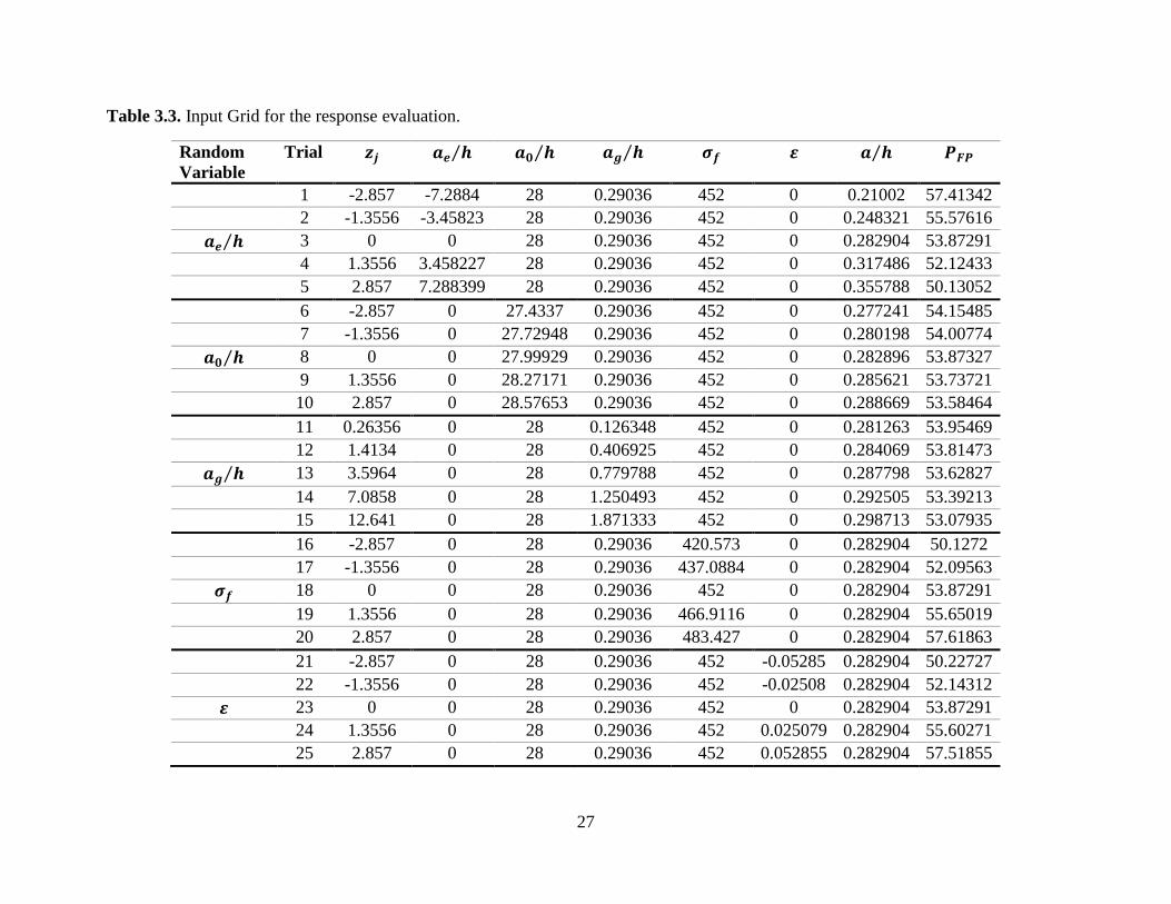
27
Table 3.3. Input Grid for the response evaluation.
Random
Variable
Trial 𝒛𝒋 𝒂𝒆 𝒉⁄ 𝒂𝟎 𝒉⁄ 𝒂𝒈 𝒉⁄ 𝝈𝒇 𝜺 𝒂 𝒉⁄ 𝑷𝑭𝑷
1 -2.857 -7.2884 28 0.29036 452 0 0.21002 57.41342
2 -1.3556 -3.45823 28 0.29036 452 0 0.248321 55.57616
𝒂𝒆 𝒉⁄ 3 0 0 28 0.29036 452 0 0.282904 53.87291
4 1.3556 3.458227 28 0.29036 452 0 0.317486 52.12433
5 2.857 7.288399 28 0.29036 452 0 0.355788 50.13052
6 -2.857 0 27.4337 0.29036 452 0 0.277241 54.15485
7 -1.3556 0 27.72948 0.29036 452 0 0.280198 54.00774
𝒂𝟎 𝒉⁄ 8 0 0 27.99929 0.29036 452 0 0.282896 53.87327
9 1.3556 0 28.27171 0.29036 452 0 0.285621 53.73721
10 2.857 0 28.57653 0.29036 452 0 0.288669 53.58464
11 0.26356 0 28 0.126348 452 0 0.281263 53.95469
12 1.4134 0 28 0.406925 452 0 0.284069 53.81473
𝒂𝒈 𝒉⁄ 13 3.5964 0 28 0.779788 452 0 0.287798 53.62827
14 7.0858 0 28 1.250493 452 0 0.292505 53.39213
15 12.641 0 28 1.871333 452 0 0.298713 53.07935
16 -2.857 0 28 0.29036 420.573 0 0.282904 50.1272
17 -1.3556 0 28 0.29036 437.0884 0 0.282904 52.09563
𝝈𝒇 18 0 0 28 0.29036 452 0 0.282904 53.87291
19 1.3556 0 28 0.29036 466.9116 0 0.282904 55.65019
20 2.857 0 28 0.29036 483.427 0 0.282904 57.61863
21 -2.857 0 28 0.29036 452 -0.05285 0.282904 50.22727
22 -1.3556 0 28 0.29036 452 -0.02508 0.282904 52.14312
𝜺 23 0 0 28 0.29036 452 0 0.282904 53.87291
24 1.3556 0 28 0.29036 452 0.025079 0.282904 55.60271
25 2.857 0 28 0.29036 452 0.052855 0.282904 57.51855

28
Fixed mean
values
26 N/A 0 28 0.29036 452 0 0.282904 53.87291
Note: zj denotes the Gauss Laguerre and Gauss Hermite points.

29
As many significant figures as possible are shown in all the tables in case these problems in case
the problems are to be repeated. The next step is to calculate the mean (𝜌𝑖) and the mean square
(휃𝑖) of an 𝑖𝑡ℎ cut function is approximated as a weighted sum (Table 3.4). Then the MDRM
approximation is used to calculate the statistical moment of the response function (Table 3.5).
Table 3.4. Output Grid for each cut function evaluation.
Random
Variable
Trial 𝒘𝒋 𝑷𝑭𝑷 𝒘𝒋 × 𝑷𝑭𝑷 𝝆𝒊 𝒘𝒋 × 𝑷𝑭𝑷𝟐 𝜽𝒊
1 1.13E-02 57.41342 0.65 37.11
2 0.22208 55.57616 12.34 685.94
𝒂𝒆 𝒉⁄ 3 0.53333 53.87291 28.73 53.86 1547.88 2902.59
4 0.22208 52.12433 11.58 603.38
5 1.13E-02 50.13052 0.56 28.29
6 1.13E-02 54.15485 0.61 33.01
7 0.22208 54.00774 11.99 647.77
𝒂𝟎 𝒉⁄ 8 0.53333 53.87327 28.73 53.87 1547.90 2902.30
9 0.22208 53.73721 11.93 641.30
10 1.13E-02 53.58464 0.60 32.32
11 0.52176 53.95469 28.15 1518.90
12 0.39867 53.81473 21.45 1154.56
𝒂𝒈 𝒉⁄ 13 7.59E-02 53.62827 4.07 53.87 218.41 2902.23
14 3.61E-03 53.39213 0.19 10.30
15 2.34E-05 53.07935 0.00 0.07
16 1.13E-02 50.1272 0.56 28.29
17 0.22208 52.09563 11.57 602.72
𝝈𝒇 18 0.53333 53.87291 28.73 53.87 1547.88 2904.02
19 0.22208 55.65019 12.36 687.77
20 1.13E-02 57.61863 0.65 37.37
21 1.13E-02 50.22727 0.57 28.40
22 0.22208 52.14312 11.58 603.81
𝜺 23 0.53333 53.87291 28.73 53.87 1547.88 2903.93
24 0.22208 55.60271 12.35 686.60
25 1.13E-02 57.51855 0.65 37.24
Fixed
mean
value
26 N/A 53.87291
Note: wj denotes the Gauss Laguerre and Gauss Hermite weights.

30
Table 3.5. Statistical Moments of the response.
𝑷𝑭𝑷 MDRM (26 Trials) MCS (106 Simulations) Relative Error
(%)
First Moment 53.8609 54.1319 0.5
Second Moment 2905.918 2935.205 0.998
Standard Deviation 2.2188 2.2237 0.22
COV 0.04119 0.04108 0.268
Note: Relative Error (%) = |𝑀𝐶𝑆−𝑀𝐷𝑅𝑀|
𝑀𝐶𝑆× 100
Table 3.5 shows the agreeability of these two methods. The relative errors are all within 1% thus
proving that the MDRM is a very good alternative to the high computational cost of MCS.
The output responses obtained using MDRM are combined with the MaxEnt principle with
fractional moment constraints, in order to estimate the response probability distribution. Table 3.6
provides the Lagrange multipliers (𝜆𝑖) and the fractional exponents (𝛼𝑖) which are used to estimate
the probability distribution of the response. The number of fractional moments used are m=2, m=3,
and m=4.
Table 3.6. MaxEnt parameters for failure pressure.
Fractional
Moments
Entropy i 0 1 2 3 4
𝜆𝑖 704.381 -175.621 0.04756
m=2 2.2061 𝛼𝑖 0.4025 2.0544
𝑀𝑋𝛼𝑖 2.765E-09 78167.41
𝜆𝑖 704.379 50.8772 -138.566 49.1863
m=3 2.2060 𝛼𝑖 -2.7479 0.8101 1.0137
𝑀𝑋𝛼𝑖 1.398E+08 1.029E-07 7.878E+06
𝜆𝑖 704.378 22.6168 47.3913 0.03417 -114.8718
m=4 2.2060 𝛼𝑖 1.0743 -4.4391 1.5810 0.7581
𝑀𝑋𝛼𝑖 3.556E-08 0.8104 2.918E-07 0.02064
The estimated probability distribution of the failure pressure is compared to the MCS (Figure 3.3).
Then the probability of failure is estimated by plotting the probability of exceedance (POE). From

31
these two figures it is seen that MDRM provides highly accurate approximation for almost the
entire range of the output response distribution (Figure 3.4).
Cubature was done using the 5 formulas stated earlier. With Formula 1, 32 points were used to
determine the mean and standard deviation, Formula 2 required the use of 43 points. Formula 3
and 4 both used 51 points, and Formula 5 used 42 points.
Data points were simulated using equation (3.2) and a probability paper plot was done. From the
probability paper plot, it was determined that a Normal distribution most accurately depicted the
probability density function for equation (3.2). Once the means and standard deviations were found
using the cubature method, the shape and scale factors were calculated and a MCS of 5000
simulations was done to determine the PDF and POE of each Formula (1, 2, 3, 4, and 5). Table 3.7
compares the means and standard deviations of the Cubature Formulas, MCS and MDRM.
Table 3.7. Means and Standard Deviations of the response.
𝑷𝑭𝑷 MDRM
(26
Trials)
MCS
(106
Trials)
Formula
1
Formula
2
Formula
3
Formula
4
Formula
5
Mean 53.8609 54.1319 53.8602 32.88 53.8604 53.8604 53.245
St. Dev 2.2188 2.2237 2.2341 16.9785 2.2340 2.2340 2.1676
M_RE(%) 0.5 N/A 0.502 39.26 0.502 0.502 1.64
S_RE(%) 0.22 N/A 0.468 663.5 0.463 0.463 2.53
Note: M_RE is the mean relative error and S_RE is the standard deviation relative error,
compared to MCS, where Relative Error (%) = |𝑀𝐶𝑆−𝑥|
𝑀𝐶𝑆× 100
From Table 3.7 it is seen that Formula 1, 3 and 4 give the closest values to MCS whereas Formula
5 is not as close. Formula 2 is not close at all, there is definitely some error that results in the values
being so far off. A possible error is that the formula was not applied correctly or was interpreted
incorrectly. Formula 1 was selected as the “best” cubature formula in terms of being able to
efficiently be able to achieve the statistical moments with the highest accuracy for multiple
32
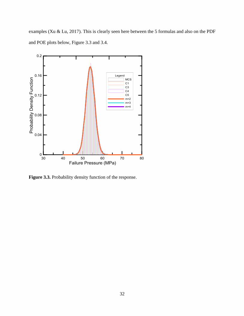
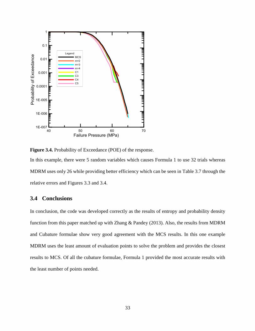
examples (Xu & Lu, 2017). This is clearly seen here between the 5 formulas and also on the PDF
and POE plots below, Figure 3.3 and 3.4.
Figure 3.3. Probability density function of the response.
33
Figure 3.4. Probability of Exceedance (POE) of the response.
In this example, there were 5 random variables which causes Formula 1 to use 32 trials whereas
MDRM uses only 26 while providing better efficiency which can be seen in Table 3.7 through the
relative errors and Figures 3.3 and 3.4.
3.4 Conclusions
In conclusion, the code was developed correctly as the results of entropy and probability density
function from this paper matched up with Zhang & Pandey (2013). Also, the results from MDRM
and Cubature formulae show very good agreement with the MCS results. In this one example
MDRM uses the least amount of evaluation points to solve the problem and provides the closest
results to MCS. Of all the cubature formulae, Formula 1 provided the most accurate results with
the least number of points needed.

34
4 MDRM for Uncertainty Analysis
4.1 Introduction
Uncertainty analysis investigates the uncertainty of variables that are used in the analysis or
decision-making problems in which observations and models represent the knowledge base. In
other words, uncertainty analysis aims to determine the uncertainty of the variable and the type of
random variable (epistemic or aleatory).
The objective of this chapter is to examine the applicability, accuracy of the MDRM and
comparing it to MCS and Cubature Formulae to determine what method is the “best.” This problem
will first be solved considering that all random variables are simply uncertain with no specific
designation as either epistemic or aleatory and the second time it will be solved considering one
random variable is epistemic while another is aleatory.
4.1.1 Organization
The organization of this chapter is as follows. Section 4.2 presents a simply uncertain problem of
a time to leak for a pipe. This is an equation based problem where no distinction is made for the
random variables as to whether they are aleatory or epistemic. This problem is done using MDRM,
MCS and Cubature methods and the results are compared. Section 4.3 solves the same problem as
Section 4.2 but this time one random variable is designated as aleatory and another is designated
as epistemic. This time the problem is only done using MDRM and MCS and the results are
compared. Finally, the conclusions are summarized in Section 4.4.

35
4.2 Simple Uncertain Problems
4.2.1 Time to Leak for a Pipe Problem
Consider the following simple model for the time to leak for a pipe, for example from stress
corrosion cracking, as:
𝑇𝐿 = 𝑇𝐼 +𝑊
𝑅
(4.1)
where 𝑇𝐿 is the time to leak (months), 𝑇𝐼 is the time to crack initiation (months), 𝑊 is the wall
thickness (mm), and 𝑅 is the crack growth rate (mm/month). 𝑊
𝑅 represents the time it takes for an
initiated crack to grow through the pipe wall, which results in a leak. Assuming all variables are
deterministic and known precisely, this problem can be solved directly without any uncertainty.
However, in reality this is not the case, many of the parameters are unknown and hence described
as uncertain or random variables. (Jyrkama & Pandey, 2016)
There are two types of random variables, epistemic and aleatory. An aleatory uncertainty is one
that is presumed to be the intrinsic randomness of a phenomenon. An epistemic uncertainty is one
that is presumed as being caused by lack of knowledge (data) (Ditlevsen & Kiureghian, 2009).
Figure 4.1 shows the difference between a first order random variable probabilistic model
definition and a second order random variable probabilistic model definition.

36
Figure 4.1. First vs second order random variable probabilistic model definition.
This problem will first be solved considering that all random variables are simply uncertain with
no specific designation as either epistemic or aleatory, this is a first order random variable
probabilistic model definition. Table 4.1 defines each variable in equation (4.1).
Table 4.1. Variables.
Variable Type of Distribution Parameters of Distribution
𝑻𝑰 Weibull (3,480 months) – (shape, scale)
𝑾 Constant 40 mm
𝑹 Normal (5 mm/month, 1 mm/month) – (mean, st.dev)
This problem was solved using Monte Carlo Simulation (MCS), the Multiplicative Dimensional
Reduction Method (MDRM) and the 5 Cubature formulas.

37
Using MCS, 1,000,000 simulations were done for each random variable and each corresponding
time to leak was calculated. Figure 4.2 shows the cumulative distribution of time to leak, 𝑇𝐿. The
mean and standard deviation were calculated as 437.0078 and 155.6737 respectively.
Figure 4.2. Cumulative distribution function of time to leak.
The MDRM was done using the fifteenth order (L=15) Gauss quadrature and considering two
input random variables (n=2). An input grid is generated to evaluate the response which can be
seen in Table 4.2. The Gauss Hermite and Gauss Laguerre formulas are adopted since one random
variable follows Normal distribution and the other follows Weibull distribution. In total there are
(2 × 15) + 1 = 31 response evaluations. For each evaluation point, the other random variable is
fixed to its mean value.

38
Table 4.2. Input Grid for the response evaluation.
Random
Variable
Trial zj Ti (months) R (mm/month) W
(mm)
Tl
(months)
1 0.093308 217.7111 5 40 225.7111
2 0.492692 379.111 5 40 387.111
3 1.215595 512.2763 5 40 520.2763
4 2.26995 630.8314 5 40 638.8314
5 3.667623 740.2347 5 40 748.2347
6 5.425337 843.4321 5 40 851.4321
7 7.565916 942.3128 5 40 950.3128
Ti 8 10.12023 1038.257 5 40 1008.93
9 13.13028 1132.398 5 40 921.9758
10 16.65441 1225.794 5 40 1275.559
11 20.77648 1319.568 5 40 1342.948
12 25.62389 1415.108 5 40 1430.687
13 31.40752 1514.441 5 40 1526.229
14 38.53068 1621.226 5 40 1630.748
15 48.02609 1744.752 5 40 1752.752
16 -6.36395 428.6302 -1.36 40 399.3035
17 -5.19009 428.6302 -0.19 40 218.2075
18 -4.19621 428.6302 0.80 40 478.3943
19 -3.28908 428.6302 1.71 40 452.0094
20 -2.43244 428.6302 2.57 40 444.2091
21 -1.60671 428.6302 3.39 40 440.4181
22 -0.79913 428.6302 4.20 40 438.152
R 23 -2.32E-16 428.6302 5.00 40 436.6302
24 0.799129 428.6302 5.80 40 435.5278
25 1.60671 428.6302 6.61 40 434.6846
26 2.432437 428.6302 7.43 40 434.012
27 3.289082 428.6302 8.29 40 433.4558
28 4.196208 428.6302 9.20 40 432.9798
29 5.190094 428.6302 10.19 40 432.5555
30 6.363948 428.6302 11.36 40 432.1501
Fixed
Mean
Values
31 N/A 428.6302 5.00 40 436.6302
Note: zj denotes the Gauss Laguerre and Gauss Hermite points.
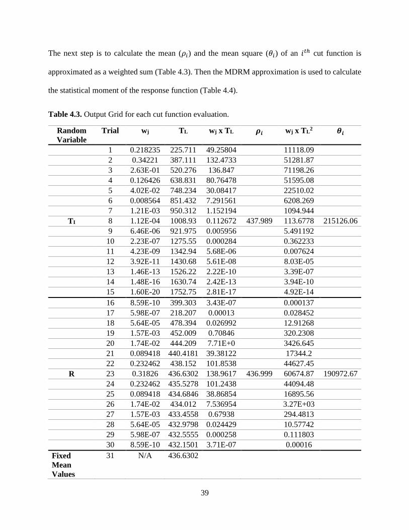
39
The next step is to calculate the mean (𝜌𝑖) and the mean square (휃𝑖) of an 𝑖𝑡ℎ cut function is
approximated as a weighted sum (Table 4.3). Then the MDRM approximation is used to calculate
the statistical moment of the response function (Table 4.4).
Table 4.3. Output Grid for each cut function evaluation.
Random
Variable
Trial wj TL wj x TL 𝝆𝒊 wj x TL2 𝜽𝒊
1 0.218235 225.711 49.25804 11118.09
2 0.34221 387.111 132.4733 51281.87
3 2.63E-01 520.276 136.847 71198.26
4 0.126426 638.831 80.76478 51595.08
5 4.02E-02 748.234 30.08417 22510.02
6 0.008564 851.432 7.291561 6208.269
7 1.21E-03 950.312 1.152194 1094.944
TI 8 1.12E-04 1008.93 0.112672 437.989 113.6778 215126.06
9 6.46E-06 921.975 0.005956 5.491192
10 2.23E-07 1275.55 0.000284 0.362233
11 4.23E-09 1342.94 5.68E-06 0.007624
12 3.92E-11 1430.68 5.61E-08 8.03E-05
13 1.46E-13 1526.22 2.22E-10 3.39E-07
14 1.48E-16 1630.74 2.42E-13 3.94E-10
15 1.60E-20 1752.75 2.81E-17 4.92E-14
16 8.59E-10 399.303 3.43E-07 0.000137
17 5.98E-07 218.207 0.00013 0.028452
18 5.64E-05 478.394 0.026992 12.91268
19 1.57E-03 452.009 0.70846 320.2308
20 1.74E-02 444.209 7.71E+0 3426.645
21 0.089418 440.4181 39.38122 17344.2
22 0.232462 438.152 101.8538 44627.45
R 23 0.31826 436.6302 138.9617 436.999 60674.87 190972.67
24 0.232462 435.5278 101.2438 44094.48
25 0.089418 434.6846 38.86854 16895.56
26 1.74E-02 434.012 7.536954 3.27E+03
27 1.57E-03 433.4558 0.67938 294.4813
28 5.64E-05 432.9798 0.024429 10.57742
29 5.98E-07 432.5555 0.000258 0.111803
30 8.59E-10 432.1501 3.71E-07 0.00016
Fixed
Mean
Values
31 N/A 436.6302

40
Note: wj denotes the Gauss Laguerre and Gauss Hermite weights.
Table 4.4. Statistical Moments of the response.
TL MDRM (31 Trials) MCS (106 Simulations) Relative Error
(%)
First Moment 438.36 437.0078 0.309
Second Moment 215494.80 215210.1181 0.132
Standard Deviation 152.76 155.6737 1.87
COV 0.3485 0.3562 2.16
Note: Relative Error (%) = |𝑀𝐶𝑆−𝑀𝐷𝑅𝑀|
𝑀𝐶𝑆× 100
Table 4.4 shows the agreeability of these two methods. The relative errors are all within 2% thus
proving that the MDRM is a good alternative to the high computational cost of MCS.
The output responses obtained using MDRM are combined with the MaxEnt principle with
fractional moment constraints, in order to estimate the response probability distribution. Table 4.5
provides the Lagrange multipliers (𝜆𝑖) and the fractional exponents (𝛼𝑖) which are used to estimate
the probability distribution of the response. The number of fractional moments used are m=2, m=3,
and m=4. The estimated probability distribution of the time to leak is compared to the MCS (Figure
4.3) then the probability of failure is estimated by plotting the probability of exceedance (POE).
From these two figures it is seen that MDRM provides highly accurate approximation for almost
the entire range of the output response distribution (Figure 4.4).
Table 4.5. MaxEnt parameters for time to leak.
Fractional
Moments
Entropy i 0 1 2 3 4
𝜆𝑖 22.6948 -2.4025 0.03409
m=2 6.4310 𝛼𝑖 0.4174 0.9859
𝑀𝑋𝛼𝑖 12.4727 401.8782
𝜆𝑖 5.4455 0.9562 27.2316 -1.3553
m=3 6.4306 𝛼𝑖 0.8193 -0.2335 0.7689
𝑀𝑋𝛼𝑖 144.6556 0.2463 106.2883
𝜆𝑖 20.02579 0.008981 0.00009737 1.2785 -2.3776

41
m=4 6.4306 𝛼𝑖 1.1386 -2.1609 0.08132 0.3888
𝑀𝑋𝛼𝑖 1028.4586 3.154E-06 1.6319 10.4808
Cubature was done using the 5 formulas stated earlier. With Formula 1, 8 points were used to
determine the mean and standard deviation. Formula 2 could not be used because this problem
does not have 3 or more random variables, this is the same reason Formula 5 could not be used as
well. Formula 3 and 4 both used 9 points.
Data points were simulated using equation (1) and a probability paper plot was done. From the
probability paper plot, it was determined that a Weibull distribution most accurately depicted the
probability density function for equation (1). Once the means and standard deviations were found
using the cubature method, the shape and scale factors were calculated and a MCS of 106
simulations was done to determine the PDF and POE of each formula (1, 3, and 4). Table 4.6
compares the means and standard deviations of the Cubature Formulas, MCS and MDRM.
Table 4.6. Means and Standard Deviations of the response.
TL MDRM
(31
Trials)
MCS (106
Simulations)
Formula 1 Formula 3 Formula 4
Mean 438.36 437.0078 437.03 598.21 599.14
St. Dev 152.76 155.6737 155.67 234.39 243.69
M_RE(%) 0.31 NA 0.005 36.9 37
S_RE(%) 1.87 NA 0.002 50.6 56.5
Note: M_RE is the mean relative error and S_RE is the standard deviation relative error,
compared to MCS, where Relative Error (%) = |𝑀𝐶𝑆−𝑥|
𝑀𝐶𝑆× 100
From Table 4.6 it is seen that Formula 1 gives the closest values to MCS and MDRM whereas
Formulas 3 and 4 are not close at all. Formula 1 was selected as the “best” cubature formula in
terms of being able to efficiently be able to achieve the statistical moments with the highest

42
accuracy for multiple examples (Xu & Lu, 2017) and in this case gives values that are even more
accurate than the MDRM. This is clearly seen here between the 3 formulas and also on the PDF
and POE plots below, Figure 4.3 and 4.4.
Figure 4.3. Probability Distribution of the response.

43
Figure 4.4. Probability of Exceedance (POE) of the response.
In this example there are only 3 random variables; with this low amount of random variables
Cubature formulae provide a more accurate answer than the MDRM that is also achieved more
efficiently. This is seen in the graphs above and in Table 4.6.
4.2.2 Observations
From this problem and the one solved in the previous chapter it is observed that Cubature formulae
do not match up with efficiency and accuracy of MDRM as the number of random variables
increase. The number of points needed for Cubature formulae increase exponentially as the number
of random variables increase whereas the accuracy stays the same as compared to MDRM. Since
this is the case the problems done from here on out will not be done using Cubature formulae, only
MDRM and MCS.

44
4.3 Problem with Epistemic Variable
4.3.1 Time to Leak for a Pipe Problem with Epistemic Random Variable
To show the impact of the separation of variables, as aleatory and epistemic, the time to initiation
(𝑇𝐼) is subject to epistemic uncertainty while the crack growth rate (𝑅) is subject to aleatory
uncertainty. Figure 4.5 outlines the process required to solve a problem of this nature.
Figure 4.5. Two-staged nested Monte Carlo Simulation/ Multiplicative Dimensional Reduction
Method approach involving separated aleatory and epistemic random variables

45
The time to initiation is sampled as part of the outer epistemic loop while the crack growth rate is
part of the inner aleatory loop, this is a second order random variable probabilistic model
definition. Table 4.7 defines each variable. The outcome of the second-order uncertainty is that the
probability of time to leak will be random as well. The uncertainty in the probability of the time to
leak will be further influenced by the degree of uncertainty of the distribution parameters (Duan,
Wang & Kozluk, 2015).
This was problem was also solved using both Monte Carlo Simulation (MCS) and Multiplicative
Dimensional Reduction Method (MDRM).
Table 4.7. Variables.
Variable Type of Distribution Parameters of Distribution
𝜶 Normal (3.5,0.5) – (mean, st.dev)
𝑻𝑰 Weibull (α,480 months) – (shape, scale)
𝑾 Constant 40 mm
𝑹 Normal (5 mm/month, 1 mm/month) – (mean, st.dev)
Using MCS, 100 simulations were taken for the outer loop and 104 simulations were taken for the
inner loop. To solve this problem using MCS, the outer loop values are simulated first. Then by
taking each of the 100 simulated values; 104 simulations of the time to initiation and crack growth
rate are taken, and each corresponding time to leak is calculated. Figure 4.6 shows the cumulative
distribution of time to leak, 𝑇𝐿.
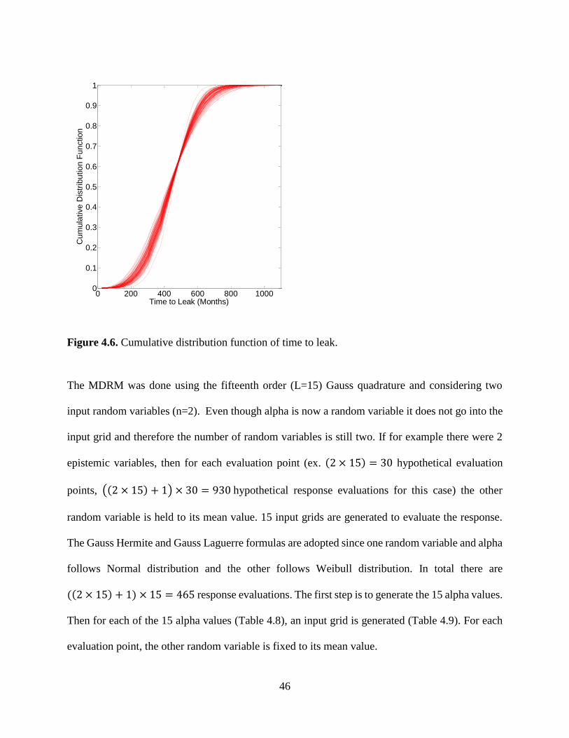
46
Figure 4.6. Cumulative distribution function of time to leak.
The MDRM was done using the fifteenth order (L=15) Gauss quadrature and considering two
input random variables (n=2). Even though alpha is now a random variable it does not go into the
input grid and therefore the number of random variables is still two. If for example there were 2
epistemic variables, then for each evaluation point (ex. (2 × 15) = 30 hypothetical evaluation
points, ((2 × 15) + 1) × 30 = 930 hypothetical response evaluations for this case) the other
random variable is held to its mean value. 15 input grids are generated to evaluate the response.
The Gauss Hermite and Gauss Laguerre formulas are adopted since one random variable and alpha
follows Normal distribution and the other follows Weibull distribution. In total there are
((2 × 15) + 1) × 15 = 465 response evaluations. The first step is to generate the 15 alpha values.
Then for each of the 15 alpha values (Table 4.8), an input grid is generated (Table 4.9). For each
evaluation point, the other random variable is fixed to its mean value.
0 200 400 600 800 10000
0.1
0.2
0.3
0.4
0.5
0.6
0.7
0.8
0.9
1
Time to Leak (Months)
Cu
mu
lative
Dis
trib
utio
n F
un
ctio
n

47
Table 4.8. Alpha values to be used.
zj 𝜶
1 -6.36394788 0.318026
2 -5.19009359 0.904953
3 -4.19620771 1.401896
4 -3.28908242 1.855459
5 -2.43243682 2.283782
6 -1.60671006 2.696645
7 -0.79912906 3.100435
8 -2.32E-16 3.5
9 0.799129068 3.899565
10 1.606710069 4.303355
11 2.432436827 4.716218
12 3.289082424 5.144541
13 4.196207711 5.598104
14 5.190093591 6.095047
15 6.363947889 6.681974
Table 4.9. Input Grid for the response evaluation of alpha 4.
Random
Variable
Trial zJ TI (months) R
(mm/month)
W
(mm)
TL
(months)
1 0.093307812 133.6836444 5 40 141.6836
2 0.49269174 327.7589841 5 40 335.759
3 1.215595412 533.259154 5 40 541.2592
4 2.269949526 746.6486117 5 40 754.6486
5 3.667622722 966.9777806 5 40 974.9778
6 5.425336627 1194.154981 5 40 1202.155
7 7.565916227 1428.577772 5 40 1436.578
TI 8 10.12022857 1671.047613 5 40 1641.721
9 13.13028248 1922.805431 5 40 1712.383
10 16.65440771 2185.670626 5 40 2235.435
11 20.7764789 2462.334124 5 40 2485.713
12 25.62389423 2756.962767 5 40 2772.542
13 31.40751917 3076.577833 5 40 3088.366
14 38.53068331 3434.884829 5 40 3444.407
15 48.02608557 3867.887286 5 40 3875.887
16 -6.363947889 426.2927152 -1.36 40 396.9661
17 -5.190093591 426.2927152 -0.19 40 215.8701
18 -4.196207711 426.2927152 0.80 40 476.0568
19 -3.289082424 426.2927152 1.71 40 449.672

48
20 -2.432436827 426.2927152 2.57 40 441.8717
21 -1.606710069 426.2927152 3.39 40 438.0807
22 -0.799129068 426.2927152 4.20 40 435.8146
R 23 -2.32E-16 426.2927152 5.00 40 434.2927
24 0.799129068 426.2927152 5.80 40 433.1903
25 1.606710069 426.2927152 6.61 40 432.3472
26 2.432436827 426.2927152 7.43 40 431.6745
27 3.289082424 426.2927152 8.29 40 431.1183
28 4.196207711 426.2927152 9.20 40 430.6423
29 5.190093591 426.2927152 10.19 40 430.2181
30 6.363947889 426.2927152 11.36 40 429.8126
Fixed
mean
values
31 N/A 426.2927152 5.00 40 434.2927
Note: zj denotes the Gauss Laguerre and Gauss Hermite points.
The next step is to calculate the mean (𝜌𝑖) and the mean square (휃𝑖) of an 𝑖𝑡ℎ cut function is
approximated as a weighted sum (Table 4.10). Then the MDRM approximation is used to calculate
the statistical moment of the response function (Table 4.11).
Table 4.10. Output Grid for each cut function evaluation for alpha 4.
Random
Variable
Trial wJ TL wj x TL 𝝆𝒊 wj x TL2 𝜽𝒊
1 0.218234886 141.68364 30.9203 4380.90
2 0.342210178 335.75898 114.900 38578.7
3 2.63E-01 541.25915 142.366 77056.9
4 0.126425818 754.64861 95.4070 71998.8
5 4.02E-02 974.97778 39.2008 38219.9
6 0.008563878 1202.1549 10.2951 12376.3
7 1.21E-03 1436.5777 1.74175 2502.17
TI 8 1.12E-04 1641.7209 0.18333 435.0261 300.990 245434
9 6.46E-06 1712.3827 0.01106 18.9421
10 2.23E-07 2235.4347 0.00049 1.11252
11 4.23E-09 2485.7133 1.05E-05 0.02612
12 3.92E-11 2772.5417 1.09E-07 0.00030
13 1.46E-13 3088.3658 4.5E-10 1.39E-06
14 1.48E-16 3444.4066 5.11E-13 1.76E-09
15 1.60E-20 3875.8872 6.2E-17 2.4E-13
16 8.59E-10 396.96608 3.41E-07 0.00013

49
17 5.98E-07 215.87005 0.00012 0.02784
18 5.64E-05 476.05681 0.02686 12.7868
19 1.57E-03 449.67198 7.05E-01 316.927
20 1.74E-02 441.87168 7.67E+0 3390.67
21 0.089417795 438.08068 39.1722 17160.5
22 0.232462294 435.81455 101.310 44152.5
R 23 0.318259518 434.29271 138.217 434.6622 60026.9 188935
24 0.232462294 433.19030 100.700 43622.4
25 0.089417795 432.347165 38.6595 16714.3
26 1.74E-02 431.674530 7.49636 3.24E+0
27 1.57E-03 431.118339 0.67571 291.313
28 5.64E-05 430.642334 0.02429 10.4635
29 5.98E-07 430.218096 0.00025 0.11059
30 8.59E-10 429.812618 3.69E-07 0.00015
Fixed
mean
values
31 N/A 434.292715
Note: wj denotes the Gauss Laguerre and Gauss Hermite weights.
To calculate the total mean of the response, the following equation is used:
Mean of means:
𝜇𝜇𝑌 = 𝐸[𝜇𝑌] ≈ 𝑚0(1−𝑚)
×∏[∑𝑤𝑗 × (𝜇𝑌𝑗)
𝐿
𝑗=1
]
𝑚
𝑖=1
(4.2)
where 𝑤𝑗 denotes the Gauss Laguerre weights corresponding to the alpha values in this case, m is
the number of distribution parameters that are random variables which in this problem is equal to
one, 𝑚0 is the mean value from the inner loop when all epistemic variables are held to their mean.
Since m=1 in this example there is no need to calculate this mean value.
Mean of mean squares:
𝜇𝜇2𝑌 = 𝐸[𝜇2𝑌] ≈ 𝑚0(1−𝑚)
×∏[∑𝑤𝑗 × (𝜇2𝑌𝑗)
𝐿
𝑗=1
]
𝑚
𝑖=1
(4.3)
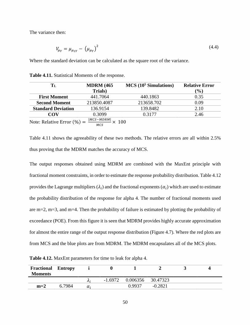
50
The variance then:
𝑉𝜇𝑌 = 𝜇𝜇2𝑌 − (𝜇𝜇𝑌)2 (4.4)
Where the standard deviation can be calculated as the square root of the variance.
Table 4.11. Statistical Moments of the response.
TL MDRM (465
Trials)
MCS (105 Simulations) Relative Error
(%)
First Moment 441.7064 440.1863 0.35
Second Moment 213850.4087 213658.702 0.09
Standard Deviation 136.9154 139.8482 2.10
COV 0.3099 0.3177 2.46
Note: Relative Error (%) = |𝑀𝐶𝑆−𝑀𝐷𝑅𝑀|
𝑀𝐶𝑆× 100
Table 4.11 shows the agreeability of these two methods. The relative errors are all within 2.5%
thus proving that the MDRM matches the accuracy of MCS.
The output responses obtained using MDRM are combined with the MaxEnt principle with
fractional moment constraints, in order to estimate the response probability distribution. Table 4.12
provides the Lagrange multipliers (𝜆𝑖) and the fractional exponents (𝛼𝑖) which are used to estimate
the probability distribution of the response for alpha 4. The number of fractional moments used
are m=2, m=3, and m=4. Then the probability of failure is estimated by plotting the probability of
exceedance (POE). From this figure it is seen that MDRM provides highly accurate approximation
for almost the entire range of the output response distribution (Figure 4.7). Where the red plots are
from MCS and the blue plots are from MDRM. The MDRM encapsulates all of the MCS plots.
Table 4.12. MaxEnt parameters for time to leak for alpha 4.
Fractional
Moments
Entropy i 0 1 2 3 4
𝜆𝑖 -1.6972 0.006356 30.47323
m=2 6.7984 𝛼𝑖 0.9937 -0.2821

51
𝑀𝑋𝛼𝑖 0.006619 0.126
𝜆𝑖 4.4183 -0.1845 33.0421 0.1544
m=3 6.7952 𝛼𝑖 0.8826 -0.5117 0.9142
𝑀𝑋𝛼𝑖 0.08386 174.6405 0.9575
𝜆𝑖 706.024 1398.961 -1200.386 733.0901 -397.4088
m=4 6.7911 𝛼𝑖 -1.2174 0.1214 0.1541 -0.3106
𝑀𝑋𝛼𝑖 2.00E+13 2.79E-11 0.6162 5674.9473
Figure 4.7. Probability of Exceedance (POE) of the response.
4.3.2 Observations
After solving this problem it was concluded that it is more efficient to just use MCS rather than
MDRM when solving an equation based uncertainty analysis with an epistemic variable. The
number of gauss points chosen for the epistemic variable (15 in this case) determines the number
of times the MDRM has to be done. There was only one epistemic variable in this problem but
0 100 200 300 400 500 600 700 800 900 1000 110010
-3
10-2
10-1
100
Time to Leak (Months)
Pro
babili
ty o
f E
xceedance

52
with more, the number of times the MDRM would have had to be done would be multiplied by the
number of epistemic variables.
4.4 Conclusion
In conclusion, after comparing all the results, it is seen that MDRM is the most logical and “best”
method to use out of the three methods used in the comparison. MDRM provides the accuracy of
MCS while decreasing the number of evaluation points significantly. While also being able to
solve for the probability density function.
Cubature formulae are also very good but their downside is that as the number of random variables
in a reliability problem increases the number of trials increase exponentially. Out of the 5 cubature
formulae the ‘best’ (most efficient and accurate) is Formula 1, which rivals the MDRM when there
are a low number of random variables (up to 3).
For MDRM use in equation based double loop problems (where the random variables are split
between aleatory and epistemic), MDRM is not a good solution as the computational effort
significantly increases based on the number of gauss quadrature points used for the aleatory
random variable.

53
5 MDRM for Fire Resistant Design of Structures
5.1 Introduction
5.1.1 Reliability Studies for Fire Resistant Design of Structures
When preparing any sort of structural design is always essential that the designer has a sense of
the level of risk associated with design they have come up with. However, current practices in the
standard fire test fail to give any information about the reliability of the structure due to a fire. The
only information given is the fire resistance under a standard fire. Prescriptive methodology is
considered to be generally over conservative (Bailey, 2006); which results in a practice in which
the structural reliability is indeterminate (Lange, Usmani and Torero, 2008) and inconsistent with
the design for other hazards such as wind and earthquake (Ellingwood, 2005).
Research that led to the formulation of performance-based methods of structural fire design has
provided an improved understanding of structural fire resistance (Jeffers et al, 2012). Apart from
the philosophical basis for the reliability-based design methodology, the probabilistic treatment of
structural performance in fire is a matter of practicality in understanding the structural responses
observed in fire resistance tests. For example, in standard fire tests, a large amount of scatter can
be observed in results from different testing facilities due to variations in heating conditions,
material properties of the specimens, magnitudes of applied loads, and the degrees of restraint
provided by the surrounding structure (Witteveen & Twilt, 1981). Furthermore, the fire resistance
of steel structures is dependent on the level of fire protection that is present. The spray-applied fire
resistant materials (SFRMs) have large variability’s due to the nature of the materials, the manner
in which they are applied in the fields and their adhesion and durability characteristics (Ryder,
Wolin and Milke, 2002). There is a lot of uncertainty in construction as well. What an engineer

54
has designed may not be what ends up being constructed due to this uncertainty. This will also
affect the fire resistance of the steel.
The topic of structural reliability in fire is not new, but a review of literature reveals that the
coverage of this topic is fairly incomplete and although progress has been made, previous work is
limited to Monte Carlo simulations (Guo & Jeffers, 2015). The work described herein will mainly
take inspiration from the work of Jeffers et al (2012). Jeffers et al (2012) utilized probabilistic
methods to evaluate the fire resistance of structures given uncertainties in key model parameters.
The proposed methodology accounted for the uncertainty stemming from the fire exposure and
structural resistance parameters. The approach is capable of giving designers the ability to
rationally evaluate the robustness provided by the various design options by providing a
quantitative measure of the structure’s reliability. (Jeffers et al, 2012) conducted an analysis of a
protected steel beam given uncertainties in the fire load and structural resistance parameters via a
sequentially coupled, stochastic finite element simulation embedded within a Monte Carlo
simulation. This research demonstrates that a probabilistic treatment of the structural fire problem
yields a wealth of data that may lead to a better understanding of the factors affecting structural
fire resistance.
5.1.2 Objective
The work in this section includes the analysis of a protected steel beam given uncertainties in the
fire load and structural resistance parameters using a performance-based design embedded within
a Multiplicative Dimensional Reduction Method (MDRM) and comparing it to Monte Carlo
simulation (MCS). MCS is overwhelmingly expensive for calculating failure probabilities that are
relatively small (Madsen et al., 2006), and therefore researchers tend to be less inclined to using
this method. This research demonstrates that the MDRM is a ‘better’ method (versus MCS) to use

55
in terms of computational effort, while also demonstrating the importance of a reliability analysis;
which is, that a reliability-based analysis of structural performance in fire provides data that
enables risk-informed decision making, which is an essential component of performance design.
5.1.3 Organization
The organization of this chapter is as follows. Section 5.2 presents the performance based approach
to solving a fire resistance problem that will be used. Section 5.3 presents the results that were
obtained by using the performance based approach. This was done using MDRM and MCS and
the results were compared. Conclusions are summarized in Section 5.4.
5.2 Performance Based Approach for Calculating Fire Resistance
The following steps must be taken in order to calculate the fire resistance time of a steel beam with
loads acting all along the beam.
First the beam properties such as beam span (𝐿), section modulus (𝑍𝑋), beam area (𝐹), beam
volume (𝑉), steel yield strength (𝑓𝑦), and the dead (𝐺𝑘) and live loads (𝑄𝑘) acting on the beam
must be known.
The calculations for the beam at room temperature must be done first to determine if the beam can
support the loads that will be placed on it. Using the dead and live loads calculate the factored
design load (𝑤𝑐) and the bending moment (𝑀𝑐𝑜𝑙𝑑∗ ) caused by this factored design load (units in
brackets):
𝑤𝑐 = 1.25𝐺𝑘 + 1.5𝑄𝑘 (𝑘𝑁
𝑚)
(5.1)
𝑀𝑐𝑜𝑙𝑑∗ =
𝑤𝑐𝐿2
8 (𝑘𝑁𝑚)
(5.2)
56
Next calculate the bending strength (𝑀𝑛) and design flexural strength (𝜙𝑀𝑛) of the beam (units
in brackets):
𝑀𝑛 = 𝑍𝑋𝑓𝑦 (𝑘𝑁𝑚) (5.3)
𝜙𝑀𝑛 (5.4)
𝜙 = 0.9
Now check if the beam will be able to support the loads by determining 𝑀𝑐𝑜𝑙𝑑∗ < 𝜙𝑀𝑛. If this is
the case then the beam is good, if not select another beam.
Now that the calculations at room temperature are done, the next step is to do the calculations for
when the beam is under a fire load. First calculate the factored design load (𝑤𝑓) and the bending
moment (𝑀𝑓𝑖𝑟𝑒∗ ) caused by this factored design load (units in brackets):
𝑤𝑓 = 𝐺𝑘 + 0.4𝑄𝑘 (𝑘𝑁
𝑚)
(5.5)
𝑀𝑓𝑖𝑟𝑒∗ =
𝑤𝑓𝐿2
8 (𝑘𝑁𝑚)
(5.6)
Next calculate the load ratio (𝑟𝑙𝑜𝑎𝑑) between the moment of the beam under fire and the bending
strength:
𝑟𝑙𝑜𝑎𝑑 =𝑀𝑓𝑖𝑟𝑒∗
𝑀𝑛
(5.7)
Using the load ratio calculate the limiting steel temperature (𝑇𝑙𝑖𝑚 − °C):
𝑇𝑙𝑖𝑚 = 905 − 690𝑟𝑙𝑜𝑎𝑑 (5.8)
From here there are two different ways to continue this problem, one is if the beam is unprotected
meaning no insulation on the beam to protect it from fire and the other is if the beam is protected
by insulation. Calculations for both cases will be shown.
57
For unprotected steel beams the time to reach the limiting temperature (also can be referred to as
the fire resistance) is calculated as follows:
𝑡 = 0.54(𝑇𝑙𝑖𝑚 − 50)
(𝐹 𝑉⁄ )0.6
(5.9)
Where 𝑡 is the time in minutes, and 𝐹 𝑉⁄ is the area to volume ratio (m-1). To determine the area
to volume ratio first calculate the area of the cross section of the beam (m2) then multiply this by
1m of length to get the volume (𝑉). Next calculate the perimeter of the cross section and multiply
it by 1m length to determine the surface area (𝐹).
For protected steel beams, the properties of the insulation must be known. The properties needed
are the thickness of the insulation(𝑑𝑖 −𝑚𝑒𝑡𝑒𝑟𝑠), the thermal conductivity of the insulation(𝑘𝑖 −
𝑊/(𝑚𝐾)), the moisture content of the insulation(𝑚 −%), and the density of the insulation(𝜌𝑖 −
𝑘𝑔
𝑚3).
The time to reach the limiting temperature is calculated as follows:
𝑡 = 40(𝑇𝑙𝑖𝑚 − 140) [𝑑𝑖 𝑘𝑖⁄
𝐹 𝑉⁄]
0.66
(5.10)
Where t is time in minutes and 𝐹 𝑉⁄ is still calculated the same as it was for unprotected steel
beams. The insulation causes there to be a time delay which can be calculated as follows:
𝑡𝑣 =𝑚𝜌𝑖𝑑𝑖
2
5𝑘𝑖
(5.11)
The total time (also can be referred to as the fire resistance) is then:
𝑡𝑡𝑜𝑡𝑎𝑙 = 𝑡 + 𝑡𝑣 (5.12)
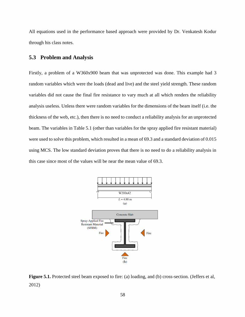
58
All equations used in the performance based approach were provided by Dr. Venkatesh Kodur
through his class notes.
5.3 Problem and Analysis
Firstly, a problem of a W360x900 beam that was unprotected was done. This example had 3
random variables which were the loads (dead and live) and the steel yield strength. These random
variables did not cause the final fire resistance to vary much at all which renders the reliability
analysis useless. Unless there were random variables for the dimensions of the beam itself (i.e. the
thickness of the web, etc.), then there is no need to conduct a reliability analysis for an unprotected
beam. The variables in Table 5.1 (other than variables for the spray applied fire resistant material)
were used to solve this problem, which resulted in a mean of 69.3 and a standard deviation of 0.015
using MCS. The low standard deviation proves that there is no need to do a reliability analysis in
this case since most of the values will be near the mean value of 69.3.
Figure 5.1. Protected steel beam exposed to fire: (a) loading, and (b) cross-section. (Jeffers et al,
2012)

59
Secondly, a problem of a W200x42 beam that is protected by spray applied fire resistant material
(SFRM) which is seen in Figure 5.1 will be solved considering 6 random variables. This beam
must achieve a 1-hr fire rating; the probability of failure will be determined. Table 5.1 defines each
variable that will be used in this problem including the constants.
Table 5.1. Variables.
Variable Type of Distribution Parameters of Distribution
𝑮𝒌 Normal (1.05 x nominal, 0.10) – (mean, COV)
Nominal Value 5.15 kN/m
𝑸𝒌 Weibull (0.24 x nominal, 0.80) – (mean, COV)
Nominal Value 3.65 kN/m
𝒇𝒚 Normal (380 MPa, 0.08) – (mean, COV)
𝒅𝒊 Lognormal (1.6 mm + nominal, 0.20) – (mean, COV)
Nominal Value 11.1 mm
𝒌𝒊 Lognormal (0.12, 0.24) – (mean, COV)
𝝆𝒊 Normal (300, 0.29) – (mean, COV)
𝑳 Constant 4.88 m
𝒁𝑿 Constant 445 x 103 mm3
𝒎 Constant 15%
This problem was solved using Monte Carlo Simulation (MCS) and the Multiplicative
Dimensional Reduction Method (MDRM).
Using MCS, 106 simulations were done for each random variable and each corresponding fire
resistance was calculated. Figure 5.1 shows the cumulative distribution of fire resistance, 𝑡𝑡𝑜𝑡𝑎𝑙.
The mean and standard deviation were calculated as 86.7014 and 20.6131 respectively.
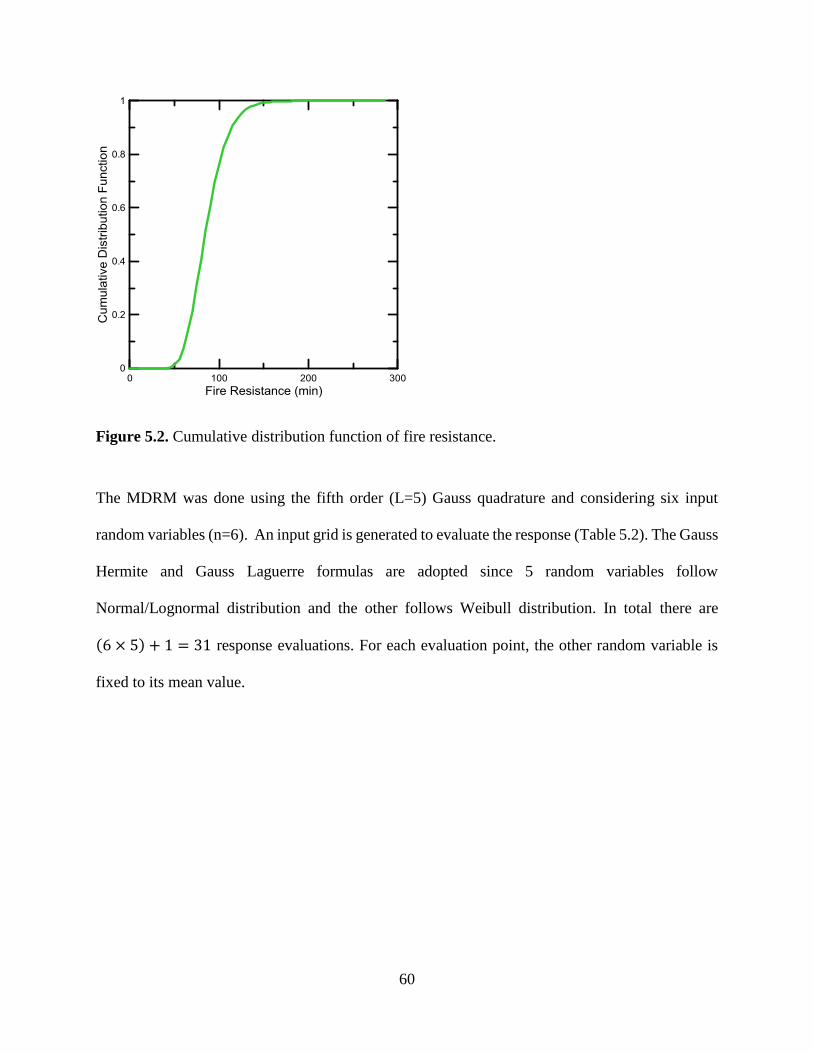
60
Figure 5.2. Cumulative distribution function of fire resistance.
The MDRM was done using the fifth order (L=5) Gauss quadrature and considering six input
random variables (n=6). An input grid is generated to evaluate the response (Table 5.2). The Gauss
Hermite and Gauss Laguerre formulas are adopted since 5 random variables follow
Normal/Lognormal distribution and the other follows Weibull distribution. In total there are
(6 × 5) + 1 = 31 response evaluations. For each evaluation point, the other random variable is
fixed to its mean value.
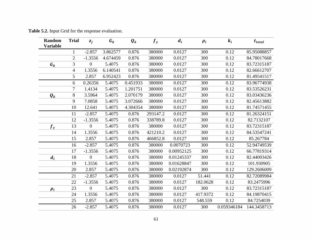
61
Table 5.2. Input Grid for the response evaluation.
Random
Variable
Trial 𝒛𝒋 𝑮𝒌 𝑸𝒌 𝒇𝒚 𝒅𝒊 𝝆𝒊 𝒌𝒊 𝒕𝒕𝒐𝒕𝒂𝒍
1 -2.857 3.862577 0.876 380000 0.0127 300 0.12 85.95088857
2 -1.3556 4.674459 0.876 380000 0.0127 300 0.12 84.78017668
𝑮𝒌 3 0 5.4075 0.876 380000 0.0127 300 0.12 83.72315187
4 1.3556 6.140541 0.876 380000 0.0127 300 0.12 82.66612707
5 2.857 6.952423 0.876 380000 0.0127 300 0.12 81.49541517
6 0.26356 5.4075 0.451933 380000 0.0127 300 0.12 83.96774938
7 1.4134 5.4075 1.201751 380000 0.0127 300 0.12 83.53526231
𝑸𝒌 8 3.5964 5.4075 2.070179 380000 0.0127 300 0.12 83.03436236
9 7.0858 5.4075 3.072666 380000 0.0127 300 0.12 82.45613882
10 12.641 5.4075 4.304354 380000 0.0127 300 0.12 81.74571455
11 -2.857 5.4075 0.876 293147.2 0.0127 300 0.12 81.26324151
12 -1.3556 5.4075 0.876 338789.8 0.0127 300 0.12 82.7132107
𝒇𝒚 13 0 5.4075 0.876 380000 0.0127 300 0.12 83.72315187
14 1.3556 5.4075 0.876 421210.2 0.0127 300 0.12 84.53547241
15 2.857 5.4075 0.876 466852.8 0.0127 300 0.12 85.267784
16 -2.857 5.4075 0.876 380000 0.0070723 300 0.12 52.94749539
17 -1.3556 5.4075 0.876 380000 0.00952125 300 0.12 66.77819314
𝒅𝒊 18 0 5.4075 0.876 380000 0.01245337 300 0.12 82.44003426
19 1.3556 5.4075 0.876 380000 0.01628847 300 0.12 101.930905
20 2.857 5.4075 0.876 380000 0.02192874 300 0.12 129.2606009
21 -2.857 5.4075 0.876 380000 0.0127 51.441 0.12 82.72089984
22 -1.3556 5.4075 0.876 380000 0.0127 182.0628 0.12 83.2475996
𝝆𝒊 23 0 5.4075 0.876 380000 0.0127 300 0.12 83.72315187
24 1.3556 5.4075 0.876 380000 0.0127 417.9372 0.12 84.19870415
25 2.857 5.4075 0.876 380000 0.0127 548.559 0.12 84.7254039
26 -2.857 5.4075 0.876 380000 0.0127 300 0.059346184 144.3458713

62
27 -1.3556 5.4075 0.876 380000 0.0127 300 0.084664032 109.6505375
𝒌𝒊 28 0 5.4075 0.876 380000 0.0127 300 0.116686476 85.55588052
29 1.3556 5.4075 0.876 380000 0.0127 300 0.160820756 66.76100387
30 2.857 5.4075 0.876 380000 0.0127 300 0.229428966 50.72781116
Fixed mean
values
31 5.4075 0.876 380000 0.0127 300 0.12 83.72315187
Note: zj denotes the Gauss Laguerre and Gauss Hermite points.

63
The next step is to calculate the mean (𝜌𝑖) and the mean square (휃𝑖) of an 𝑖𝑡ℎ cut function is
approximated as a weighted sum (Table 5.3). Then the MDRM approximation is used to calculate
the statistical moment of the response function (Table 5.4). This table also shows the relative errors
between the statistical moments obtained by MDRM and MCS which are very low showing a good
agreement between the two methods.
Table 5.3. Output Grid for each cut function evaluation.
Random
Variable
Trial 𝒘𝒋 𝒕𝒕𝒐𝒕𝒂𝒍 𝒘𝒋
× 𝒕𝒕𝒐𝒕𝒂𝒍
𝝆𝒊 𝒘𝒋
× 𝒕𝒕𝒐𝒕𝒂𝒍𝟐
𝜽𝒊
1 1.13E-02 85.95089 0.97 83.48
2 0.22208 84.78018 18.83 1596.24
𝑮𝒌 3 0.53333 83.72315 44.65 83.73 3738.41 7010.81
4 0.22208 82.66613 18.36 1517.63
5 1.13E-02 81.49542 0.92 75.05
6 0.52176 83.96775 43.81 3678.71
7 0.39867 83.53526 33.30 2781.98
𝑸𝒌 8 7.59E-02 83.03436 6.30 83.72 523.31 7008.70
9 3.61E-03 82.45614 0.30 24.54
10 2.34E-05 81.74571 0.00 0.16
11 1.13E-02 81.26324 0.92 74.62
12 0.22208 82.71321 18.37 1519.35
𝒇𝒚 13 0.53333 83.72315 44.65 83.68 3738.41 7001.58
14 0.22208 84.53547 18.77 1587.04
15 1.13E-02 85.26778 0.96 82.16
16 1.13E-02 52.9475 0.60 31.68
17 0.22208 66.77819 14.83 990.33
𝒅𝒊 18 0.53333 82.44003 43.97 83.49 3624.70 7142.90
19 0.22208 101.9309 22.64 2307.39
20 1.13E-02 129.2606 1.46 188.80
21 1.13E-02 82.7209 0.93 77.32
22 0.22208 83.2476 18.49 1539.05
𝝆𝒊 23 0.53333 83.72315 44.65 83.73 3738.41 7010.32
24 0.22208 84.1987 18.70 1574.42
25 1.13E-02 84.7254 0.96 81.12
26 1.13E-02 144.3459 1.63 235.44
27 0.22208 109.6505 24.35 2670.12
𝒌𝒊 28 0.53333 85.55588 45.63 87.01 3903.87 7828.33
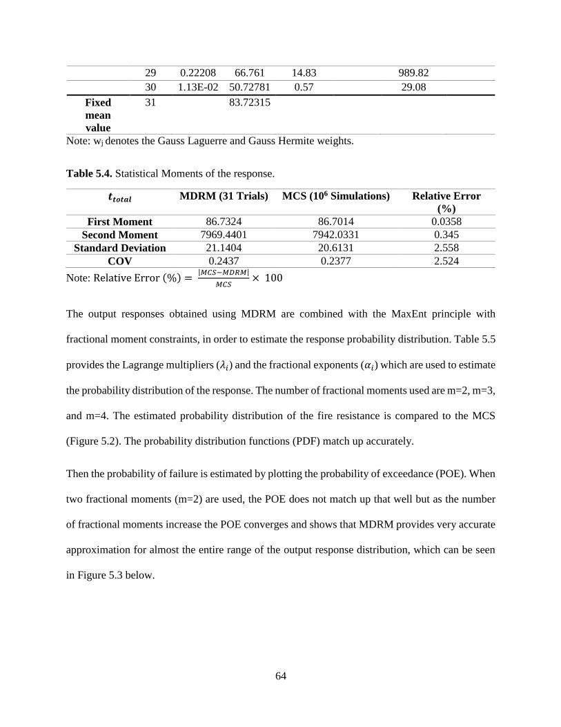
64
29 0.22208 66.761 14.83 989.82
30 1.13E-02 50.72781 0.57 29.08
Fixed
mean
value
31 83.72315
Note: wj denotes the Gauss Laguerre and Gauss Hermite weights.
Table 5.4. Statistical Moments of the response.
𝒕𝒕𝒐𝒕𝒂𝒍 MDRM (31 Trials) MCS (106 Simulations) Relative Error
(%)
First Moment 86.7324 86.7014 0.0358
Second Moment 7969.4401 7942.0331 0.345
Standard Deviation 21.1404 20.6131 2.558
COV 0.2437 0.2377 2.524
Note: Relative Error (%) = |𝑀𝐶𝑆−𝑀𝐷𝑅𝑀|
𝑀𝐶𝑆× 100
The output responses obtained using MDRM are combined with the MaxEnt principle with
fractional moment constraints, in order to estimate the response probability distribution. Table 5.5
provides the Lagrange multipliers (𝜆𝑖) and the fractional exponents (𝛼𝑖) which are used to estimate
the probability distribution of the response. The number of fractional moments used are m=2, m=3,
and m=4. The estimated probability distribution of the fire resistance is compared to the MCS
(Figure 5.2). The probability distribution functions (PDF) match up accurately.
Then the probability of failure is estimated by plotting the probability of exceedance (POE). When
two fractional moments (m=2) are used, the POE does not match up that well but as the number
of fractional moments increase the POE converges and shows that MDRM provides very accurate
approximation for almost the entire range of the output response distribution, which can be seen
in Figure 5.3 below.

65
Table 5.5. MaxEnt parameters for failure pressure.
Fractional
Moments
Entropy i 0 1 2 3 4
𝜆𝑖 705.9991 2328.6595 -2761.634
m=2 4.1396 𝛼𝑖 -0.2072 -0.1187
𝑀𝑋𝛼𝑖 1.8676 0.7455
𝜆𝑖 705.9865 -1168.1429 62.4452 585.2371
m=3 4.1391 𝛼𝑖 -0.01267 0.2164 -0.2017
𝑀𝑋𝛼𝑖 2.8492 1.6988 0.3411
𝜆𝑖 705.9864 712.1589 -3108.974 1586.1246 280.1337
m=4 4.1391 𝛼𝑖 0.08442 -0.00833 -0.08365 -0.1205
𝑀𝑋𝛼𝑖 0.7868 1.1397 1.6746 1.2813
The probabilities of failure, meaning the probability that this beam will last less than 60 minutes
during a fire, from both MCS and MDRM can be seen in Table 5.6 below.
Table 5.6. Probability of failure; probability that the steel beam will fail before 60 minutes.
𝒕𝒕𝒐𝒕𝒂𝒍 MDRM (%) MCS (%) Relative Error
(%)
Probability of
Failure
7.9654 7.2774 9.4541
Note: Relative Error (%) = |𝑀𝐶𝑆−𝑀𝐷𝑅𝑀|
𝑀𝐶𝑆× 100
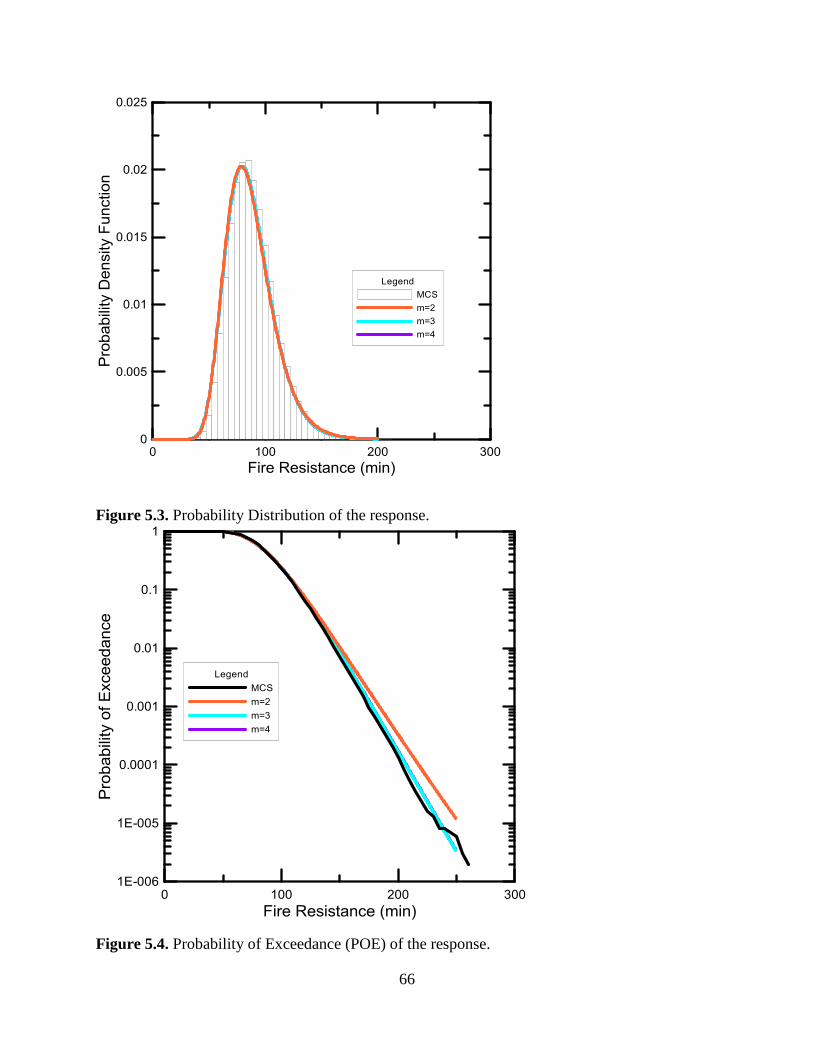
66
Figure 5.3. Probability Distribution of the response.
Figure 5.4. Probability of Exceedance (POE) of the response.

67
5.4 Conclusion
In this example MDRM only needs 31 trials compared to the 1,000,000 trials used for MCS. Even
though only 31 trials were needed the accuracy did not suffer. For MDRM the mean and standard
deviation are 86.7324 and 21.1404 respectively, and for MCS the mean and standard deviation are
86.7014 and 20.6131. Which give a relative error of 0.0358 and 2.558 for mean and standard
deviation respectively which are very low numbers that show agreeability between the two
methods.
The probability distribution function (PDF) graphs and the probability of exceedance (POE)
graphs (Figure 5.2 and 5.3) also show a good agreement between the two methods. The PDF graphs
match up very accurately The POE graphs provide a very accurate approximation for almost the
entire range of the output response distribution as the number of fractional moments increase.
When only two fractional moments are used there is not a good agreement between MCS and
MDRM but as the number of fractional moments increase the graphs converge and show good
agreement between MCS and MDRM.
The suitability of MDRM was determined by considering an application of a protected steel beam
under natural fire. The 1-h rated beam was found to have a probability of failure of 7.9654% under
natural fire exposure which indicates that the beam is likely to survive a fire for 1-h. However,
discussion is needed amongst the fire safety engineering community to determine what an
acceptable percentage for the probability of failure is so engineers can do reliability studies based
on that number.
In summary, this study shows the importance of applying a reliability analysis of structural fire
resistance which provides an enhanced understanding of the factors affecting the resistance of

68
structures to fire and offers a means for improving the design to meet performance objectives.
Which in this case is done by using the Multiplicative Dimensional Reduction Method.

69
6 MDRM for Geomechanics Problems
6.1 Introduction
6.1.1 Reliability Analysis for Geomechanics
Engineering design with a consideration of soil is a difficult task because there are many important
sources of uncertainty that could lead to over- or under-designing. Measurements of soil properties
along with detailed observation suggest considerable variability in soil properties, not only from
site to site but even within samples at a single site (Christian & Baecher, 2003).
There are multiple different ways to apply a reliability analysis such as First-Order Reliability
Method (FORM), Second Order Reliability Method (SORM), First Order Second Moment
(FOSM), or Monte Carlo Simulation (MCS). MCS is perhaps the most well-known and easiest to
implement. When the complete output distribution is of interest, MCS is the generic approach to
solve the problem (Zhang, 2013).
However as discussed previously the fact that most reliability analysis methods are
computationally expensive is the reason why there are not a lot of risk and reliability analyses done
in the field of geomechanics. Thus, the main motivation behind this research is to use the
Multiplicative Dimensional Reduction Method which is a computationally efficient, robust, and
easy to implement method that can be compared to the accuracy of MCS. Using this method for
geomechanics problems will provide evidence to support the claims of accuracy and computational
efficiency and hopefully make it so more engineers do a reliability analysis instead of a
deterministic one.
70
6.1.2 Objective
The work in this section includes 4 problems. These problems are based on solving equations and
finite element analyses. The first two problems are equation based which require substituting
random variables into the equation and the second two problems are finite element analyses which
require substituting random variables into finite element models. These problems show the
accuracy and computational efficiency of MDRM compared to MCS. MCS is overwhelmingly
expensive for calculating failure probabilities that are relatively small (Madsen et al., 2006), and
therefore researchers tend to be less inclined to using this method. This research demonstrates that
the MDRM is a ‘better’ method (versus MCS) to use in terms of computational effort. It also
demonstrates the importance of a reliability analysis. The importance is that a reliability-based
analysis of soil integrity provides data that enables risk-informed decision making.
6.1.3 Organization
The organization of this chapter is as follows. Section 6.2 presents a step by step detailed
calculation of MDRM for a 1D consolidation problem (settlement of foundation). This was
compared to MCS. Section 6.3 presents a simple 1D consolidation problem (determining degree
of consolidation) was is done using MDRM and MCS, and the results are compared. These first
two sections deal with equation based problems. Section 6.4 presents a vertical drain problem.
This problem was done using finite element analysis. The area of influence is modeled in
ABAQUS and meshed. The mesh is then output into a FORTRAN program provided by Dipanjan
Basu. This is done using MDRM and MCS and the results and computational effort are compared.
Section 6.5 presents a concrete infinite beam on an elastic foundation problem. This problem is
also done using a finite element analysis. The foundation is modeled using two different models,
the two parameter Pasternak Model and Modified Vlasov Model. Each foundation model is done

71
twice for a static and dynamic load. This is done using MDRM and MCS and the results and
computational effort are compared. Finally, Section 6.6 discusses the conclusions that were made.
6.2 Detailed Calculation Steps of MDRM
To show a step by step detailed calculation using MDRM a simple 1D consolidation problem will
be solved in which the settlement of the foundation will be determined. This problem will also
compare the accuracy of MDRM to MCS. Computational efficiency will not be looked at in this
example since only equations are used to solve the problem and not a finite element analysis. The
problem is to determine the settlement of a flexible, circular foundation of diameter 2.0 m. The
axial load is 1200 kN. The soil properties are taken as random variables which are defined in Table
6.1 below. The equations that will be used to solve this problem are:
𝑞𝑏 =𝑄
𝜋 (𝐵2)
2
(6.1)
𝑞𝑏 =1200
𝜋 (22)
2
𝑞𝑏 = 382 𝑘𝑃𝑎
and
𝑤 =𝑞𝑏𝐵(1 − 𝜇
2)
𝐸
(6.2)
Where Q is the axial load, B is the diameter of the foundation, 𝑞𝑏 is a distributed load, 𝜇 is the
Poisson’s ratio and 𝐸 is the elastic modulus of soil.
Table 6.1. Variables
Variable Type of Distribution Parameters of Distribution
𝑬 Lognormal (10500 kPa, 30%) – (mean, coefficient of variance)
𝝁 Lognormal (0.45, 7%) – (mean, coefficient of variance)

72
This problem was solved using Monte Carlo Simulation (MCS), and the Multiplicative
Dimensional Reduction Method (MDRM).
Using MCS, 10000 simulations were done for each random variable and each settlement of the
foundation was determined. The 10000 MCS values determined for E and 𝜇 were substituted into
the settlement equation to solve for the statistical moments and the probability density function.
Figure 6.1 shows the cumulative distribution of the settlement of the foundation. The mean and
standard deviation were calculated as 0.06306 and 0.01905 respectively.
Figure 6.1. Cumulative distribution function of settlement of the foundation obtained by
simulations
To use MDRM, the input grid must first be assembled. The first step to assembling the input grid
is determining the gauss quadrature that will be used for each random variable according to the
type of distribution. In this case both random variables are lognormal therefore the Probabilists'
Gauss-Hermite integration formula, weights, and points will be used. Since random variables are

73
of lognormal distribution the shape and scale parameters must be solved for using the following
equations:
휁 = √ln (1 +𝜎2
𝜇2) (shape parameter) and 𝜆 = ln(𝜇) −
1
2휁2(scale parameter)
In this case the shape and scale factors are 휁 = 0.06991 and 𝜆 = −0.8009 for poisons ratio and 휁 =
0.29356 and 𝜆 = 9.216042 for the elastic modulus of soil. For this example the MDRM was done
using the fifth order (L=5) Gauss quadrature, therefore 5 values of 𝑥𝑗 were found for each random
variable using the following equation from Table 2.1:
𝑥𝑗 = exp (𝜆 + 휁𝑧𝑗)
Trial 1 for elastic modulus of soil for example will be done as follows:
𝑥1 = exp(𝜆 + 휁𝑧1)
𝑥1 = exp(9.216042 + 0.29356 (−2.85697))
𝑥1 = 4347.4279
Trial 4 for poisons ratio for example will be done as follows:
𝑥4 = exp(𝜆 + 휁𝑧4)
𝑥4 = exp(−0.8009 + 0.06991 (1.35563))
𝑥4 = 0.4935
This step will be done a total of 5 times for each random variable which will result in 10 trials plus
one more trial at which the random variables will both be kept at their mean. In total, there are
(2 × 5) + 1 = 11 response evaluations. For each evaluation point, the other random variable is
fixed to its mean value. The corresponding values of each trial will then be substituted back into

74
the equation that is being solved to determine the response values of each trial. An example of this
step is shown below and the input grid is shown in Table 6.2:
𝑤 =𝑞𝑏𝐵(1 − 𝜇1
2)
𝐸1
𝑤 =383 × 2(1 − 0.452)
4347.4279
𝑤 = 0.1401 m
Table 6.2. Input Grid for the response evaluation.
Random
Variable
Trial 𝑬 𝝁 Settlement of
Foundation (m)
1 4347.427999 0.45 0.140149532
2 6755.357941 0.45 0.090193592
𝑬 3 10057.17599 0.45 0.060582613
4 14972.82452 0.45 0.040693057
5 23265.8917 0.45 0.026188122
6 10500 0.36762298 0.062928377
7 10500 0.40831033 0.060631235
𝝁 8 10500 0.44890154 0.058099465
9 10500 0.49352802 0.055039295
10 10500 0.54815014 0.050899239
Fixed mean
value
11 10500
0.45 0.058027619
Note: zj denotes the Gauss Hermite points.
The next step is to calculate the mean (𝜌𝑖) and the mean square (휃𝑖) of an 𝑖𝑡ℎ cut function which
is approximated as a weighted sum. To do this the response values must first be multiplied by the
corresponding Gaussian weights and the response values squared must also be multiplied by the
Gauussian weights which are shown in Table 6.3. Using these values the first moment and second
moments for each variable can be calculated. The first moment of the modulus of elasticity of soil
can be calculated as follows using equation 2.12:

75
𝜌𝐸 =∑𝑤𝑗
5
𝑗=1
ℎ(𝐸𝑗 , 𝜇0)
𝜌𝐸 = 0.00157766 + 0.02003019 + 0.03231052 + 0.00903711 + 0.0002948
𝜌𝐸 = 0.063250295
Similarly, the second moment of the poisons ratio can be calculated as follows using equation
2.13:
휃𝜇 =∑𝑤𝑗
5
𝑗=1
[ℎ(𝐸0, 𝜇𝑗)]2
휃𝜇 = (4.45775E − 05)+ 0.000816399 + 0.001800281 + 0.000672752 + (2.91639E − 05)
휃𝜇 = 0.003363173
These values as well as all the other moments can be found in Table 6.3.

76
Table 6.3. Output Grid for each cut function evaluation.
Random
Variable
Trial 𝒘𝒋 Settlement
(𝒘) 𝒘𝒋 ×𝒘 𝝆𝒊 𝒘𝒋 ×𝒘
𝟐 𝜽𝒊
1 1.13E-02 0.140149532 0.00157766 0.000221109
2 0.22208 0.090193592 0.02003019 0.001806595
𝑬 3 0.53333 0.060582613 0.03231052 0.063250295 0.001957456 0.004360628
4 0.22208 0.040693057 0.00903711 0.000367748
5 1.13E-02 0.026188122 0.0002948 7.72025E-06
6 1.13E-02 0.062928377 0.00070838 4.45775E-05
7 0.22208 0.060631235 0.01346498 0.000816399
𝝁 8 0.53333 0.058099465 0.03098619 0.057955656 0.001800281 0.003363173
9 0.22208 0.055039295 0.01222313 0.000672752
10 1.13E-02 0.050899239 0.00057297 2.91639E-05
Fixed Mean
Value
11 0.058027619
Note: wj denotes the Gauss Hermite weights.

77
Then the MDRM approximation is used to calculate the statistical moments of the response
function. The mean of the response is calculated as follows using equation 2.14:
𝜇𝑌 = 𝐸[𝑌] ≈ ℎ0(1−𝑛) ×∏𝜌𝑖
𝑛
𝑖=1
𝜇𝑌 = 0.058027619(1−2) × 0.063250295 × 0.057955656
𝜇𝑌 = 0.063171855
The mean square of the response is calculated as follows using equation 2.15:
𝜇2𝑌 = 𝐸[𝑌2] ≈ ℎ0
(2−2𝑛) ×∏휃𝑖
𝑛
𝑖=1
𝜇2𝑌 = 0.058027619(2−2(2)) × 0.004360628 × 0.003363173
𝜇2𝑌 = 0.004355407
Using the mean and mean square the variance can then be calculated using equation 2.16:
𝑉𝑌 = 𝜇2𝑌 − (𝜇𝑌)2
𝑉𝑌 = 0.004355407 − (0.063171855)2
𝑉𝑌 = 0.000364724
The standard deviation can then be calculated by taking the square root of the variance. Table 6.4
shows all the statistical moments of the response from both MDRM and MCS. This table also
shows the relative errors between the two methods which are very low showing a good agreement
between the two methods.

78
Table 6.4. Statistical Moments of the response.
Settlement of
Foundation (m)
MDRM (11 Trials) MCS (10000
Simulations)
Relative Error
(%)
First Moment 0.063171855 0.063069361 0.16251105
Second Moment 0.004355407 0.004340762 0.337377552
Standard Deviation 0.019097745 0.019053035 0.234658499
COV 0.302314138 0.302096537 0.072030391
Note: Relative Error (%) = |𝑀𝐶𝑆−𝑀𝐷𝑅𝑀|
𝑀𝐶𝑆× 100
The output responses obtained using MDRM are combined with the MaxEnt principle with
fractional moment constraints, in order to estimate the response probability distribution. The
MaxEnt code must be used here to solve for the Lagrange multipliers (𝜆𝑖) and the fractional
exponents (𝛼𝑖). The program should be ran about 100 times or more, in this example the program
was ran 100 times. Each time the fractional exponent must be randomized to find the minimum
function evaluation. The fractional exponents and Lagrange multipliers for the lowest function
evaluation must then be saved. Using these fractional exponents and Lagrange multipliers the
fractional moments, 𝜆0, and estimated PDF can be calculated. The fractional moment for m=2 and
i=1 can be calculated as follows using equation 2.20:
𝑀𝑌𝛼1 = 𝐸[𝑌𝛼1] ≈ ℎ0
𝛼1(1−𝑛)∏∑𝑤𝑗
𝐿
𝑗=1
[ℎ𝑖(𝑥𝑗)]𝛼1
𝑛
𝑖=1

79
𝑀𝑌𝛼1 = 0.058027619−1.3151(1−2)
× [1.13E − 02(0.140149532)−1.3151 + 0.22208(0.090193592)−1.3151
+ 0.53333(0.060582613)−1.3151 + 0.22208(0.040693057)−1.3151 + 1.13E
− 02(0.026188122)−1.3151]
× [1.13E − 02(0.062928377)−1.3151 + 0.22208(0.060631235)−1.3151
+ 0.53333(0.058099465)−1.3151 + 0.22208(0.055039295)−1.3151 + 1.13E
− 02(0.050899239)−1.3151]
𝑀𝑌𝛼1 = 0.0002096
𝜆0 can then be solved substituting the fractional exponents and Lagrange multipliers and then
performing the following integral using equation 2.22:
𝜆0 = ln [ ∫ exp(−∑𝜆𝑖
𝑚
𝑖=1
∞
0
𝑦𝛼𝑖)𝑑𝑦]
Using the fractional exponents, Lagrange multipliers and 𝜆0 the estimated PDF can be obtained by
expanding the following equation and substituting a range of values, y, so a graph can be plotted
using equation 2.23:
𝑓𝑌(𝑦) = exp(−∑𝜆𝑖
𝑚
𝑖=0
𝑦𝛼𝑖)
Table 6.5 provides the Lagrange multipliers (𝜆𝑖) and the fractional exponents (𝛼𝑖) which are used
to estimate the probability distribution of the response. The number of fractional moments used
are m=2, m=3, and m=4.
80
Table 6.5. MaxEnt parameters for failure pressure.
Fractional
Moments
Entropy i 0 1 2 3 4
𝜆𝑖 -9.5702 6.98E-02 125.1533
m=2 -2.6043 𝛼𝑖 -1.3151 1.2561
𝑀𝑋𝛼𝑖 2.10E-04 3.74E-04
𝜆𝑖 81.23629 279.8922 -289.151 1.07E-04
m=3 -2.6051 𝛼𝑖 0.4681 0.2113 -2.6841
𝑀𝑋𝛼𝑖 1.43E-04 1.20E+03 4.38E-02
𝜆𝑖 -13.1159 2723.707 6.86E-01 -1593.96 229.9049
m=4 -2.6032 𝛼𝑖 5.3209 -0.7794 3.5828 1.4461
𝑀𝑋𝛼𝑖 2.18E+02 1.34E-04 3.80E-01 1.41E-05
The estimated probability distribution of the settlement of the foundation is compared to the MCS
(Figure 6.2). The probability distribution functions (PDF) match up spot on and there are no
differences in the PDF plots between the two methods.
Then the probability of failure is estimated by plotting the probability of exceedance (POE) (Figure
6.3). The POE matches up very well. The MDRM plots converge to the MCS plot, this can be seen
as the fractional moment increase it gets closer to the MCS plot.
In conclusion it can be seen that MDRM provides the same accuracy of MCS in a lesser amount
of trials/simulations.

81
Figure 6.2. Probability Density Function of the response.
Figure 6.3. Probability of Exceedance (POE) of the response.

82
6.3 Simple 1D Consolidation Problem
Another equation based example is done to provide further evidence that the Multiplicative
Dimensional Reduction Method provides similar accuracy to that of Monte Carlo Simulation. This
example is a simple 1D consolidation problem will be solved in which the consolidation of soil
after 2 years will be determined. Computational efficiency will not be looked at in this example
since only equations are used to solve the problem and not a finite element analysis. The problem
will be solved based on the following Fourier series solution:
𝑢(𝑧, 𝑡) = ∑2𝑢𝑖𝑛𝜋
∞
𝑛=1
(1 − cos 𝑛𝜋) sin (𝑛𝜋𝑧
2𝐻𝑑𝑟) exp(
−𝑛2𝜋2𝑐𝑣𝑡
4𝐻𝑑𝑟2 )
(6.3)
From this Fourier series solution, the following equation for time factor can be derived, which will
be used in calculations:
𝑇 =𝑐𝑣𝑡
𝐻𝑑𝑟2
(6.4)
The equation used for degree of consolidation can be derived from the following equation:
𝑈(𝑇) = 1 −∫ 𝑢(𝑧, 𝑡)𝐻𝑑𝑟0
𝑑𝑧
𝐻𝑑𝑟𝑢𝑖
(6.5)
The equation for degree of consolidation is:
𝑈 = √4𝑇
𝜋
(6.6)
Where T is the time factor, 𝑐𝑣 is the coefficient of consolidation in m2/years, t is the time in years,
𝐻𝑑𝑟 is the maximum vertical distance the water has to travel in m, and U is the degree of
consolidation.

83
For this problem two random variables were taken which are 𝑐𝑣 and the height of the soil layer, H.
These random variables along with the constants are defined in Table 6.6.
Table 6.6. Variables
Variable Type of Distribution Parameters of Distribution
𝑯 Normal (3, 0.15306) – (mean, standard deviation)
𝒄𝒗 Lognormal (0.2, 0.1) – (mean, standard deviation)
𝒕 Constant 2 years
This problem was solved using Monte Carlo Simulation (MCS), and the Multiplicative
Dimensional Reduction Method (MDRM).
Using MCS, 10000 simulations were done for each random variable and each degree of
consolidation after 2 years was determined. The 10000 MCS values determined for H and
𝑐𝑣, substituted into the time factor and degree of consolidation equations to determine the
moments, and the probability density function. Figure 6.4 shows the cumulative distribution of the
degree of consolidation after 2 years. The mean and standard deviation were calculated as 0.4626
and 0.1143 respectively.

84
Figure 6.4. Cumulative distribution function of degree of consolidation after 2 years.
The MDRM was done using the fifth order (L=5) Gauss quadrature and considering two input
random variables (n=2). An input grid is generated to evaluate the response (Table 4). The Gauss
Hermite formulas are adopted since the random variables follow normal and lognormal
distribution. In total there are (2 × 5) + 1 = 11 response evaluations. For each evaluation point,
the other random variable is fixed to its mean value. The values for H and 𝑐𝑣 shown below in Table
6.7 are then taken and substituted into the time factor and degree of consolidation equations to
determine the results.
Table 6.7. Input Grid for the response evaluation.
Random
Variable
Trial 𝒄𝒗 𝑯 Degree of Consolidation
after 2 yrs
1 0.046393244 3 0.22914278
2 0.09429105 3 0.3266736
𝒄𝒗 3 0.178885438 3 0.44995211
4 0.339374733 3 0.61975288
85
5 0.689755597 3 0.8835404
6 0.2 2.56269605 0.55695224
7 0.2 2.79250639 0.51111765
𝑯 8 0.2 3 0.47576643
9 0.2 3.20749361 0.44498897
10 0.2 3.43730395 0.41523802
Fixed mean
value
11 0.2 3 0.47576643
Note: zj denotes the Gauss Hermite points.
The next step is to calculate the mean (𝜌𝑖) and the mean square (휃𝑖) of an 𝑖𝑡ℎ cut function is
approximated as a weighted sum (Table 6.8). Then the MDRM approximation is used to calculate
the statistical moment of the response function (Table 6.9). This table also shows the relative errors
between the statistical moments obtained by MDRM and MCS which are very low showing a good
agreement between the two methods.

86
Table 6.8. Output Grid for each cut function evaluation.
Random
Variable
Trial 𝒘𝒋 U after 2
years
𝒘𝒋 × 𝑼 𝝆𝒊 𝒘𝒋 ×𝑼𝟐 𝜽𝒊
1 1.13E-02 0.22914278 2.58E-03 5.91E-04
2 0.22208 0.3266736 7.25E-02 2.37E-02
𝒄𝒗 3 0.53333 0.44995211 2.40E-01 0.462680824 1.08E-01 0.226354031
4 0.22208 0.61975288 1.38E-01 8.53E-02
5 1.13E-02 0.8835404 9.95E-03 8.79E-03
6 1.13E-02 0.55695224 6.27E-03 3.49E-03
7 0.22208 0.51111765 1.14E-01 5.80E-02
𝑯 8 0.53333 0.47576643 2.54E-01 0.477016615 1.21E-01 0.228145722
9 0.22208 0.44498897 9.88E-02 4.40E-02
10 1.13E-02 0.41523802 4.67E-03 1.94E-03
Fixed Mean
Value
11 0.47576643
Note: wj denotes the Gauss Hermite weights.

87
Table 6.9. Statistical Moments of the response.
Degree of Consolidation
after 2 yrs
MDRM (11 Trials) MCS (10000
Simulations)
Relative
Error (%)
First Moment 0.463897 0.462612 0.277595071
Second Moment 0.228146 0.227083 0.46794171
Standard Deviation 0.11378 0.114338 0.487661837
COV 0.245271 0.247157 0.763138473
Note: Relative Error (%) = |𝑀𝐶𝑆−𝑀𝐷𝑅𝑀|
𝑀𝐶𝑆× 100
The output responses obtained using MDRM are combined with the MaxEnt principle with
fractional moment constraints, in order to estimate the response probability distribution. Table 6.10
provides the Lagrange multipliers (𝜆𝑖) and the fractional exponents (𝛼𝑖) which are used to estimate
the probability distribution of the response. The number of fractional moments used are m=2, m=3,
and m=4.
Table 6.10. MaxEnt parameters for failure pressure.
Fractional
Moments
Entropy i 0 1 2 3 4
𝜆𝑖 -11.2039 1.5641 14.8481
m=2 -0.7982 𝛼𝑖 -1.3151 1.2561
𝑀𝑋𝛼𝑖 0.106699958 0.122852389
𝜆𝑖 128.3307 165.6812 -288.819 0.03882
m=3 -0.7993 𝛼𝑖 0.4681 0.2113 -2.6841
𝑀𝑋𝛼𝑖 0.09723 8.2904 0.4202
𝜆𝑖 -7.5808 1.6903 12.3769 -7.9791 6.526
m=4 -0.7984 𝛼𝑖 -3.9118 1.3176 -3.735 -3.6569
𝑀𝑋𝛼𝑖 0.636994 4.899731 19.81892 0.393433
The estimated probability distribution of the degree of consolidation after 2 years is compared to
the MCS (Figure 6.5). The probability distribution functions (PDF) match up spot on and there are
no differences in the PDF plots between the two methods.

88
Then the probability of failure is estimated by plotting the probability of exceedance (POE) (Figure
6.6). The POE matches up very well. The MDRM plots converge to the MCS plot, this can be seen
as the fractional moment increase it gets closer to the MCS plot.
In conclusion it can be seen that MDRM provides the same accuracy of MCS in a lesser amount
of trials/simulations.
Figure 6.5. Probability Density Function of the response.

89
Figure 6.6. Probability of Exceedance (POE) of the response.
6.4 Vertical Drains
Techniques such as preloading are needed to increase the strength and stiffness of soils due the
fact that thick deposits of soft, saturated clay have low shear strength, high compressibility and
low hydraulic conductivity (Prezzi & Basu, 2007). Installation of vertical drains are combined with
preloading to speed up the consolidation process and hence increase the strength gain rate (Holtz,
1987; Balasubramaniam, Alfaro and Bergado, 1993). The prefabricated vertical drains (PVDs) are
installed at regular intervals in a square, rectangular or triangular pattern (Anderson and Bergado,
1996). The area of influence of PVDs installed in triangular and square patterns is shown below in
Figure 6.7 (left) and (right). PVDs are installed using closed-ended mandrels; the installation of
the PVDs significantly disturbs the surrounding soil which creates a disturbed zone around the
PVD (Prezzi & Basu, 2007). The disturbed zone consists of two zones: the smear zone and the
transition zone (Anderson and Bergado, 1996; Miura, Park and Madhav, 1993). Since the mandrel
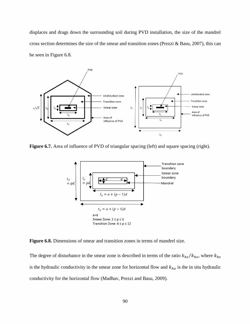
90
displaces and drags down the surrounding soil during PVD installation, the size of the mandrel
cross section determines the size of the smear and transition zones (Prezzi & Basu, 2007), this can
be seen in Figure 6.8.
Figure 6.7. Area of influence of PVD of triangular spacing (left) and square spacing (right).
Figure 6.8. Dimensions of smear and transition zones in terms of mandrel size.
The degree of disturbance in the smear zone is described in terms of the ratio 𝑘ℎ𝑠 𝑘ℎ𝑜⁄ , where 𝑘ℎ𝑠
is the hydraulic conductivity in the smear zone for horizontal flow and 𝑘ℎ𝑜 is the in situ hydraulic
conductivity for the horizontal flow (Madhav, Prezzi and Basu, 2009).

91
A reliability analysis is done to determine the time factor at 90% consolidation using PVDs in
square and triangular pattern. To solve this problem the method from (Prezzi & Basu, 2007;
Madhav, Prezzi and Basu, 2009) is used. A quadrant of the total area of influence of a PVD is
modeled and meshed in ABAQUS (since the total are of influence of a PVD is symmetrical only
one quadrant has to be modeled). Next the connectivity matrix of the elements and the coordinates
of all the nodes are output from ABAQUS and then input into the code provided by Dr. Dipanjan
Basu. The code is ran and the time factor at 90% consolidation is taken as the output. This code
employs a finite element analysis to solve the problem. Two random variables are assumed those
being the spacing and the degree of disturbance in the smear zone (𝑘𝑠𝑚𝑒𝑎𝑟𝑟𝑎𝑡𝑖𝑜). All variables used
for both patterns are shown in the Table 6.11 below.
Table 6.11. Variables
Variable Type of Distribution Parameters of Distribution
𝑺𝒑𝒂𝒄𝒊𝒏𝒈 Normal (1, 0.10204) – (mean, standard deviation)
𝒌𝒔𝒎𝒆𝒂𝒓𝒓𝒂𝒕𝒊𝒐 Lognormal (0.35, 0.12755) – (mean, standard deviation)
The PVD size is taken as 100 mm X 4 mm. The mandrel size is taken as 125 mm X 50 mm (a X
d). The smear zone is therefore taken as 175 mm X 100 mm (𝑙𝑥 × 𝑙𝑦) where p is 2. The transition
zone is therefore taken as 525 mm X 450 mm (𝑡𝑥 × 𝑡𝑦) where p is 9. The boundary condition
where the drain is located is a dirichlet boundary where u=0.
6.4.1 Triangular Pattern
The triangular pattern is modeled in ABAQUS by taking one quadrant of Figure 6.7 (left).
This problem was solved using Monte Carlo Simulation (MCS), and the Multiplicative
Dimensional Reduction Method (MDRM).

92
Using MCS, 1000 simulations were done for each random variable and each corresponding time
factor (TF) at 90% consolidation was determined. One MCS value of spacing and one MCS value
of 𝑘𝑠𝑚𝑒𝑎𝑟𝑟𝑎𝑡𝑖𝑜 were used in the method explained above 1000 times. Figure 6.9 shows the
cumulative distribution of the time factor at 90% consolidation. The mean and standard deviation
were calculated as 1.5964 and 0.4795 respectively.
Figure 6.9. Cumulative distribution function of time factor at 90% consolidation.
The MDRM was done using the fifth order (L=5) Gauss quadrature and considering two input
random variables (n=2). An input grid is generated to evaluate the response (Table 6.12). The
Gauss Hermite formulas are adopted since the random variables follow normal and lognormal
distribution. In total there are (2 × 5) + 1 = 11 response evaluations. For each evaluation point,
the other random variable is fixed to its mean value. These 11 response evaluations are then used
in the method explained above.

93
Table 6.12. Input Grid for the response evaluation.
Random
Variable
Trial 𝒌𝒔𝒎𝒆𝒂𝒓𝒓𝒂𝒕𝒊𝒐 𝑺𝒑𝒂𝒄𝒊𝒏𝒈 Time Factor @
90% Consolidation
1 0.119901116 1 3.46623961
2 0.20374465 1 2.249047331
𝒌𝒔𝒎𝒆𝒂𝒓𝒓𝒂𝒕𝒊𝒐 3 0.328842933 1 1.52981011
4 0.530750987 1 1.040849378
5 0.901890477 1 0.701820931
6 0.35 0.70846403 1.320787826
7 0.35 0.86167093 1.395962018
𝑺𝒑𝒂𝒄𝒊𝒏𝒈 8 0.35 1 1.455066313
9 0.35 1.13832907 1.499681671
10 0.35 1.29153597 1.541008111
Fixed mean
value
11 0.35 1 1.455066313
Note: zj denotes the Gauss Hermite points.
The next step is to calculate the mean (𝜌𝑖) and the mean square (휃𝑖) of an 𝑖𝑡ℎ cut function is
approximated as a weighted sum (Table 6.13). Then the MDRM approximation is used to calculate
the statistical moment of the response function (Table 6.14). This table also shows the relative
errors between the statistical moments obtained by MDRM and MCS which are very low showing
a good agreement between the two methods.

94
Table 6.13. Output Grid for each cut function evaluation.
Random
Variable
Trial 𝒘𝒋 TF @ 90%
Consolidation
𝒘𝒋 × 𝑻𝑭 𝝆𝒊 𝒘𝒋 × 𝑻𝑭𝟐 𝜽𝒊
1 1.13E-02 3.46623961 3.90E-02 0.135250795
2 0.22208 2.249047331 0.499468431 1.123328142
𝒌𝒔𝒎𝒆𝒂𝒓𝒓𝒂𝒕𝒊𝒐 3 0.53333 1.52981011 0.815893626 1.59343374 1.248162318 2.752880158
4 0.22208 1.040849378 0.23115183 0.240594238
5 1.13E-02 0.701820931 0.007900398 0.005544665
6 1.13E-02 1.320787826 0.014868109 0.019637617
7 0.22208 1.395962018 0.310015245 0.432769507
𝑺𝒑𝒂𝒄𝒊𝒏𝒈 8 0.53333 1.455066313 0.776030517 1.4513103 1.129175863 2.107782992
9 0.22208 1.499681671 0.333049305 0.499467939
10 1.13E-02 1.541008111 0.017347128 0.026732065
Fixed Mean
Value
11 1.455066313
Note: wj denotes the Gauss Hermite weights.

95
Table 6.14. Statistical Moments of the response.
Time Factor at 90%
Consolidation
MDRM (11 Trials) MCS (1000
Simulations)
Relative Error
(%)
First Moment 1.589321 1.596464 0.447467824
Second Moment 2.740612 2.778651 1.368973749
Standard Deviation 0.463328 0.479535 3.379704986
COV 0.291526 0.300373 2.945416955
Note: Relative Error (%) = |𝑀𝐶𝑆−𝑀𝐷𝑅𝑀|
𝑀𝐶𝑆× 100
The output responses obtained using MDRM are combined with the MaxEnt principle with
fractional moment constraints, in order to estimate the response probability distribution. Table 6.15
provides the Lagrange multipliers (𝜆𝑖) and the fractional exponents (𝛼𝑖) which are used to estimate
the probability distribution of the response. The number of fractional moments used are m=2, m=3,
and m=4.
Table 6.15. MaxEnt parameters for failure pressure.
Fractional
Moments
Entropy i 0 1 2 3 4
𝜆𝑖 -6.9398 5.35E+00 2.3371
m=2 0.58519 𝛼𝑖 -1.3151 1.2561
𝑀𝑋𝛼𝑖 2.7104 2.2629
𝜆𝑖 -12.6714 1.70E-07 7.7814 5.6248
m=3 0.5850 𝛼𝑖 -2.7381 -1.1538 0.8298
𝑀𝑋𝛼𝑖 1.9074 0.4814 1.1843
𝜆𝑖 -6.5882 6.9676 4.08E-01 7.5366 -7.5838
m=4 0.58486 𝛼𝑖 -1.1669 1.1727 0.7549 0.3005
𝑀𝑋𝛼𝑖 14.1052 0.3257 2.4957 4.6067
The estimated probability distribution of the displacement at midspan is compared to the MCS
(Figure 6.10). The probability distribution functions (PDF) match up spot on and there are no
differences between the two methods.

96
Then the probability of failure is estimated by plotting the probability of exceedance (POE) (Figure
6.11). The POE matches up very well. The MDRM plots converge to the MCS plot, this can be
seen as the fractional moment increase it gets closer to the MCS plot.
Figure 6.10. Probability Density Function of the response.

97
Figure 6.11. Probability of Exceedance (POE) of the response.
6.4.1.1 Computational Time
The difference in computational time is the main advantage of MDRM. For the analysis of time
factor at 90% consolidation due to vertical drains, simulation of 1000 iterations of this process
takes 66.7 hours on a personal computer with Intel I5-4690 4th Generation Processor and 8GB of
RAM. MDRM approximation based on 11 finite element analyses takes 19 minutes and MaxEnt
method requires 3.3 minutes. Thus the total time taken by MDRM is 22.3 minutes which is only
0.56% of the time taken by MCS. The reason why it takes so long to do the MCS is that it is
required to change the FE model each time due to the random variability of the spacing 1000 times
versus only having to change it 11 times for MDRM.
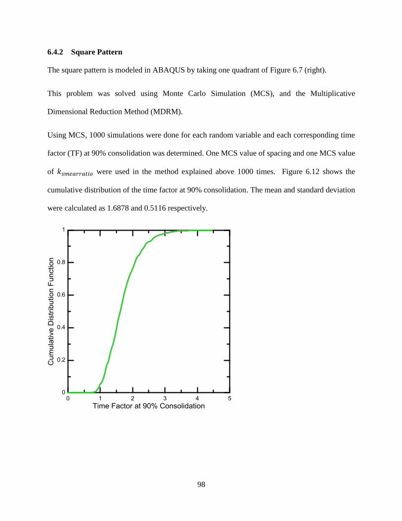
98
6.4.2 Square Pattern
The square pattern is modeled in ABAQUS by taking one quadrant of Figure 6.7 (right).
This problem was solved using Monte Carlo Simulation (MCS), and the Multiplicative
Dimensional Reduction Method (MDRM).
Using MCS, 1000 simulations were done for each random variable and each corresponding time
factor (TF) at 90% consolidation was determined. One MCS value of spacing and one MCS value
of 𝑘𝑠𝑚𝑒𝑎𝑟𝑟𝑎𝑡𝑖𝑜 were used in the method explained above 1000 times. Figure 6.12 shows the
cumulative distribution of the time factor at 90% consolidation. The mean and standard deviation
were calculated as 1.6878 and 0.5116 respectively.
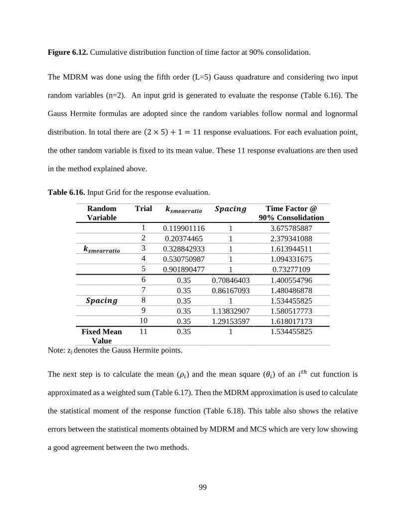
99
Figure 6.12. Cumulative distribution function of time factor at 90% consolidation.
The MDRM was done using the fifth order (L=5) Gauss quadrature and considering two input
random variables (n=2). An input grid is generated to evaluate the response (Table 6.16). The
Gauss Hermite formulas are adopted since the random variables follow normal and lognormal
distribution. In total there are (2 × 5) + 1 = 11 response evaluations. For each evaluation point,
the other random variable is fixed to its mean value. These 11 response evaluations are then used
in the method explained above.
Table 6.16. Input Grid for the response evaluation.
Random
Variable
Trial 𝒌𝒔𝒎𝒆𝒂𝒓𝒓𝒂𝒕𝒊𝒐 𝑺𝒑𝒂𝒄𝒊𝒏𝒈 Time Factor @
90% Consolidation
1 0.119901116 1 3.675785887
2 0.20374465 1 2.379341088
𝒌𝒔𝒎𝒆𝒂𝒓𝒓𝒂𝒕𝒊𝒐 3 0.328842933 1 1.613944511
4 0.530750987 1 1.094331675
5 0.901890477 1 0.73277109
6 0.35 0.70846403 1.400554796
7 0.35 0.86167093 1.480486878
𝑺𝒑𝒂𝒄𝒊𝒏𝒈 8 0.35 1 1.534455825
9 0.35 1.13832907 1.580517773
10 0.35 1.29153597 1.618017173
Fixed Mean
Value
11 0.35 1 1.534455825
Note: zj denotes the Gauss Hermite points.
The next step is to calculate the mean (𝜌𝑖) and the mean square (휃𝑖) of an 𝑖𝑡ℎ cut function is
approximated as a weighted sum (Table 6.17). Then the MDRM approximation is used to calculate
the statistical moment of the response function (Table 6.18). This table also shows the relative
errors between the statistical moments obtained by MDRM and MCS which are very low showing
a good agreement between the two methods.

100
Table 6.17. Output Grid for each cut function evaluation.
Random
Variable
Trial 𝒘𝒋 TF @ 90%
Consolidation
𝒘𝒋 × 𝑻𝑭 𝝆𝒊 𝒘𝒋 × 𝑻𝑭𝟐 𝜽𝒊
1 1.13E-02 3.675785887 4.14E-02 0.152097851
2 0.22208 2.379341088 0.528404069 1.257253512
𝒌𝒔𝒎𝒆𝒂𝒓𝒓𝒂𝒕𝒊𝒐 3 0.53333 1.613944511 0.860765026 1.681825399 1.389226989 3.070577365
4 0.22208 1.094331675 0.243029178 0.265954528
5 1.13E-02 0.73277109 0.008248804 0.006044485
6 1.13E-02 1.400554796 0.015766045 0.02208121
7 0.22208 1.480486878 0.328786526 0.486764137
𝑺𝒑𝒂𝒄𝒊𝒏𝒈 8 0.53333 1.534455825 0.818371325 1.532139303 1.255754648 2.348834522
9 0.22208 1.580517773 0.351001387 0.554763931
10 1.13E-02 1.618017173 0.018214019 0.029470596
Fixed Mean
Value
11 1.534455825
Note: wj denotes the Gauss Hermite weights.

101
Table 6.18. Statistical Moments of the response.
Time Factor at 90%
Consolidation
MDRM (11 Trials) MCS (1000
Simulations)
Relative Error
(%)
First Moment 1.679286 1.687858 0.507846486
Second Moment 3.063118 3.110617 1.526999277
Standard Deviation 0.493067 0.511617 3.625754186
COV 0.293617 0.303116 3.133822709
Note: Relative Error (%) = |𝑀𝐶𝑆−𝑀𝐷𝑅𝑀|
𝑀𝐶𝑆× 100
The output responses obtained using MDRM are combined with the MaxEnt principle with
fractional moment constraints, in order to estimate the response probability distribution. Table 6.19
provides the Lagrange multipliers (𝜆𝑖) and the fractional exponents (𝛼𝑖) which are used to estimate
the probability distribution of the response. The number of fractional moments used are m=2, m=3,
and m=4.
Table 6.19. MaxEnt parameters for failure pressure.
Fractional
Moments
Entropy i 0 1 2 3 4
𝜆𝑖 -6.7922 2.34E+00 5.472684636
m=2 0.64701 𝛼𝑖 1.1947 -1.3936
𝑀𝑋𝛼𝑖 8.1071 0.7406
𝜆𝑖 91.1141 -123.0873 32.3623 0.6149
m=3 0.64637 𝛼𝑖 0.1699 0.5669 -3.4351
𝑀𝑋𝛼𝑖 14.0842 1.6025 0.5044
𝜆𝑖 -2.7193 3.3673 4.57E-01 0.1385 -0.2073
m=4 0.64662 𝛼𝑖 -1.7205 3.0296 4.9947 4.8097
𝑀𝑋𝛼𝑖 7.6822 6.5451 1.3302 0.4057
The estimated probability distribution of the displacement at midspan is compared to the MCS
(Figure 6.13). The probability distribution functions (PDF) match up spot on and there are no
differences between the two methods.

102
Then the probability of failure is estimated by plotting the probability of exceedance (POE) (Figure
6.14). The POE matches up very well. The MDRM plots converge to the MCS plot, this can be
seen as the fractional moment increase it gets closer to the MCS plot.
Figure 6.13. Probability Density Function of the response.

103
Figure 6.14. Probability of Exceedance (POE) of the response.
6.4.2.1 Computational Time
The difference in computational time is the main advantage of MDRM. For the analysis of time
factor at 90% consolidation due to vertical drains, simulation of 1000 iterations of this process
takes 58.3 hours on a personal computer with Intel I5-4690 4th Generation Processor and 8GB of
RAM. MDRM approximation based on 11 finite element analyses takes 15 minutes and MaxEnt
method requires 3.23 minutes. Thus the total time taken by MDRM is 18.23 minutes which is only
0.52% of the time taken by MCS. The reason why it takes so long to do the MCS is that it is
required to change the FE model each time due to the random variability of the spacing 1000 times
versus only having to change it 11 times for MDRM.
6.5 Concrete Infinite Beam on an Elastic Foundation
A problem of a concrete infinite beam on an elastic foundation will be solved to provide another
example of the computational efficiency provided by MDRM. A MATLAB computer program

104
that uses a finite element analysis, developed by a colleague, Hesham Elhuni, was used to solve
this problem.
Random variables were inputted into this program and probability density functions and
probability of exceedance graphs were generated using both Monte Carlo Simulation and
Multiplicative Dimensional Reduction Method to compare results and computational effort.
This program solves for the displacement of a concrete infinite beam on an elastic foundation.
There are two foundation models used, the Modified Vlasov Model (continuum model) and the
two parameter Pasternak Foundation Model (discrete model which is done by modelling the soil
using springs). These two models are used twice once as a static problem and once as a dynamic
problem.
The differential equation that is solved by this MATLAB computer program by a finite element
analysis is:
𝐸𝐼𝑑4𝑤
𝑑𝑥4− 2𝑡𝑠
𝑑2𝑤
𝑑𝑥2+ 𝑘𝑤 + 𝜌
𝑑2𝑤
𝑑𝑡2+ 𝑐
𝑑𝑤
𝑑𝑡= 𝑃𝛿(𝑥 − 𝑣𝑡)
(6.7)
Where w is the transverse deflection of beam (m), E is the modulus of elasticity of the beam (N/m2),
I is the moment of inertia of the beam (m4), 𝜌 is the mass per unit length of the beam-foundation
system contributing in vibration (kg/m), c is the coefficient of viscous damping of the system per
unit length of the beam (N-sec/m2), P is the applied force (N). If a dynamic problem is being solved
(moving load) then the P is the applied moving concentrated force (N) and a dirac delta function
(𝛿) is added. Where v is the velocity of the moving load (m/sec), x is the horizontal distance
measured from left side of the beam (m), and t is the time (sec) (Basu & Elhuni, 2017). When
solving the two parameter Pasternak Model:

105
𝑡𝑠 = 𝑡𝑠 (6.8)
𝑘 = 𝑘𝑠 (6.9)
Where 𝑡𝑠 is the shear parameter of soil (N) and 𝑘𝑠 is the Winkler spring constant (N/m2) (Basu &
Elhuni, 2017). Figure 6.15 shows the two parameter Pasternak Model. When solving using the
Modified Vlasov Model:
2𝑡𝑠 = ∫𝐸𝑠𝑏
2(1 + 𝜇𝑠)
𝐻
0
∅2𝑑𝑧
(6.10)
𝑘 = ∫𝐸𝑠𝑏(1 − 𝜇𝑠)
(1 + 𝜇𝑠)(1 − 2𝜇𝑠)
𝐻
0
(𝑑∅
𝑑𝑧)2
𝑑𝑧
(6.11)
Where 𝐸𝑠 is the modulus of elasticity of the soil, H and b are the height and width of the soil model
respectively, 𝜇𝑠 is the Poisson’s ratio of the soil, and ∅(𝑧) is a function assumed by Vlasov for
the vertical displacement of the soil. Additional simplifications and derivations of the above two
formulas are found in (Girija Vallabhan and Das, 1991). Figure 6.16 shows the Modified Vlasov
Model.
Figure 6.15. Two Parameter Pasternak Model: static load (left) and dynamic load (right)

106
Figure 6.16. Modified Vlasov Model: static load (left) and dynamic load (right)
6.5.1 Static Continuum Problem
This problem will be solved considering that the elastic modulus of soil (𝐸𝑠) and the Poisson's
ratio (𝜇𝑠) are random variables using a Modified Vlasov Model as seen in Figure 6.16 (left). The
beam was considered to be 20 m in length, with a 100 kN static load at the midpoint. 20 m of soil
was considered on both sides of the beam. Table 6.20 defines each random variable used in this
problem.
Table 6.20. Variables.
Variable Type of Distribution Parameters of Distribution
𝑬𝒔 Lognormal (40, 30%) – (mean, coefficient of variance)
𝝁𝒔 Lognormal (0.4, 7%) – (mean, coefficient of variance)
This problem was solved using Monte Carlo Simulation (MCS), and the Multiplicative
Dimensional Reduction Method (MDRM).
Using MCS, 1000 simulations were done for each random variable and each corresponding
midspan displacement was calculated. Figure 6.17 shows the cumulative distribution of the

107
displacement at midspan. The mean and standard deviation were calculated as 0.000753 and
0.000221 respectively.
Figure 6.17. Cumulative distribution function of displacement at midspan.
The MDRM was done using the fifth order (L=5) Gauss quadrature and considering two input
random variables (n=2). An input grid is generated to evaluate the response (Table 6.21). The
Gauss Hermite formulas are adopted since the random variables follow lognormal distribution. In
total there are (2 × 5) + 1 = 11 response evaluations. For each evaluation point, the other random
variable is fixed to its mean value. Each response evaluation is then substituted into the MATLAB
computer program to determine the displacement at midspan.

108
Table 6.21. Input Grid for the response evaluation.
Random
Variable
Trial 𝑬𝒔 𝝁𝒔 Displacement at
Midspan (m)
1 16561630.47 0.4 0.00145803
2 25734696.92 0.4 0.001023777
𝑬𝒔 3 38313051.41 0.4 0.000743463
4 57039331.49 0.4 0.000540816
5 88631968.37 0.4 0.000381271
6 40000000 0.32677598 0.00095386
7 40000000 0.36294252 0.000852139
𝝁𝒔 8 40000000 0.39902359 0.000722201
9 40000000 0.43869157 0.000533294
10 40000000 0.48724457 0.00018069
Fixed mean
value
11 40000000 0.4 0.000718202
Note: zj denotes the Gauss Hermite points.
The next step is to calculate the mean (𝜌𝑖) and the mean square (휃𝑖) of an 𝑖𝑡ℎ cut function is
approximated as a weighted sum (Table 6.22). Then the MDRM approximation is used to calculate
the statistical moment of the response function (Table 6.23). This table also shows the relative
errors between the statistical moments obtained by MDRM and MCS which are very low showing
a good agreement between the two methods.
109
Table 6.22. Output Grid for each cut function evaluation.
Random
Variable
Trial 𝒘𝒋 Displacement
at Midspan
(m)
𝒘𝒋 × 𝒅𝒊𝒔𝒑 𝝆𝒊 𝒘𝒋 × 𝒅𝒊𝒔𝒑𝟐 𝜽𝒊
1 1.13E-02 0.00145803 1.64E-05 2.39E-08
2 0.22208 0.00102378 0.00022736 2.32766E-07
𝑬𝒔 3 0.53333 0.00074346 0.000396511 0.00076468 2.94792E-07 6.18079E-07
4 0.22208 0.00054082 0.000120104 6.49545E-08
5 1.13E-02 0.00038127 4.29196E-06 1.6364E-09
6 1.13E-02 0.00095386 1.07376E-05 1.02422E-08
7 0.22208 0.00085214 0.000189243 1.61261E-07
𝝁𝒔 8 0.53333 0.0007222 0.000385171 0.00070562 2.78171E-07 5.13203E-07
9 0.22208 0.00053329 0.000118434 6.31602E-08
10 1.13E-02 0.00018069 2.03402E-06 3.67528E-10
Fixed Mean
Value
11 0.0007182
Note: wj denotes the Gauss Hermite weights.
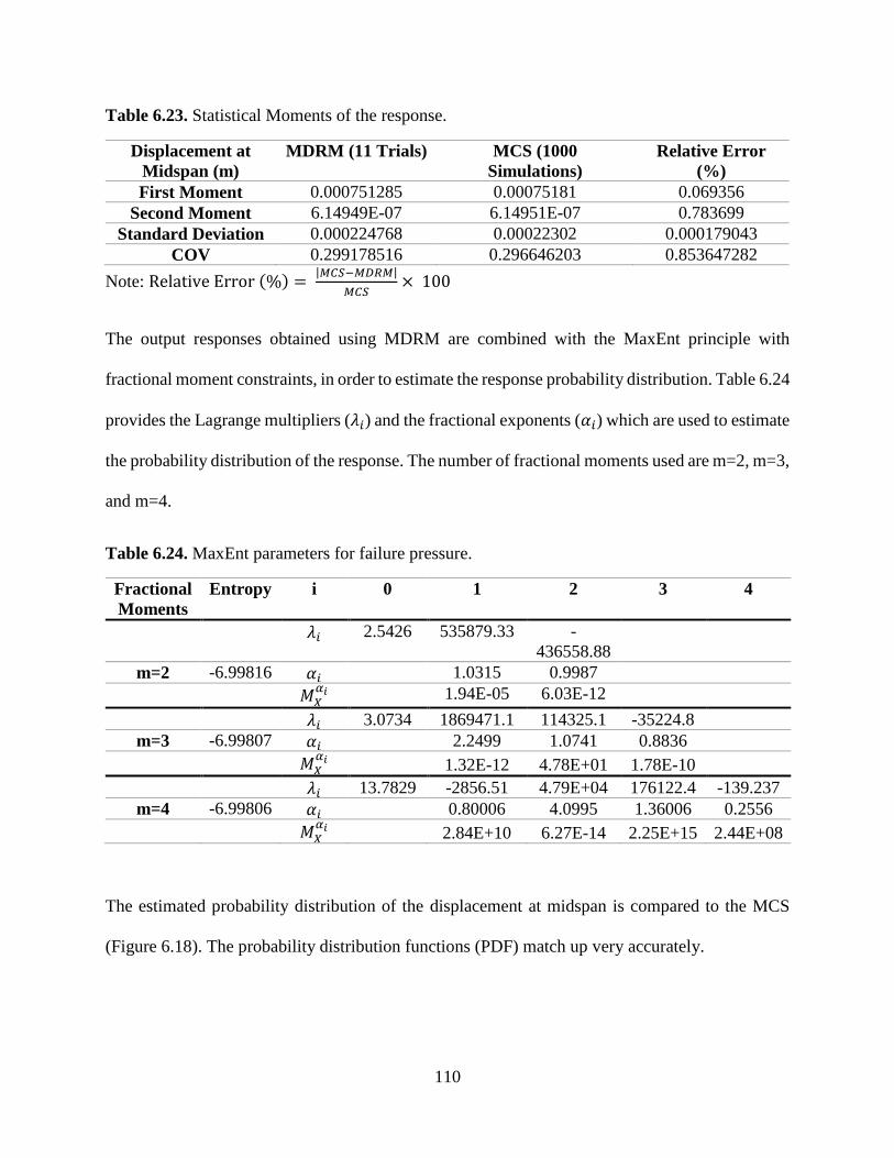
110
Table 6.23. Statistical Moments of the response.
Displacement at
Midspan (m)
MDRM (11 Trials) MCS (1000
Simulations)
Relative Error
(%)
First Moment 0.000751285 0.00075181 0.069356
Second Moment 6.14949E-07 6.14951E-07 0.783699
Standard Deviation 0.000224768 0.00022302 0.000179043
COV 0.299178516 0.296646203 0.853647282
Note: Relative Error (%) = |𝑀𝐶𝑆−𝑀𝐷𝑅𝑀|
𝑀𝐶𝑆× 100
The output responses obtained using MDRM are combined with the MaxEnt principle with
fractional moment constraints, in order to estimate the response probability distribution. Table 6.24
provides the Lagrange multipliers (𝜆𝑖) and the fractional exponents (𝛼𝑖) which are used to estimate
the probability distribution of the response. The number of fractional moments used are m=2, m=3,
and m=4.
Table 6.24. MaxEnt parameters for failure pressure.
Fractional
Moments
Entropy i 0 1 2 3 4
𝜆𝑖 2.5426 535879.33 -
436558.88
m=2 -6.99816 𝛼𝑖 1.0315 0.9987
𝑀𝑋𝛼𝑖 1.94E-05 6.03E-12
𝜆𝑖 3.0734 1869471.1 114325.1 -35224.8
m=3 -6.99807 𝛼𝑖 2.2499 1.0741 0.8836
𝑀𝑋𝛼𝑖 1.32E-12 4.78E+01 1.78E-10
𝜆𝑖 13.7829 -2856.51 4.79E+04 176122.4 -139.237
m=4 -6.99806 𝛼𝑖 0.80006 4.0995 1.36006 0.2556
𝑀𝑋𝛼𝑖 2.84E+10 6.27E-14 2.25E+15 2.44E+08
The estimated probability distribution of the displacement at midspan is compared to the MCS
(Figure 6.18). The probability distribution functions (PDF) match up very accurately.

111
Then the probability of failure is estimated by plotting the probability of exceedance (POE) (Figure
6.19). The POE matches up very accurately and as the number of fractional moments increase the
MDRM (m=4) matches closer to the MCS.
Figure 6.18. Probability Density Function of the response.
Figure 6.19. Probability of Exceedance (POE) of the response.

112
6.5.1.1 Computational Time
The difference in computational time is the main advantage of MDRM. For the analysis of a
concrete infinite beam on an elastic foundation, simulation of 1000 iterations of the computer
program takes 2.75 hours on a personal computer with Intel I5-4690 4th Generation Processor and
8GB of RAM. MDRM approximation based on 11 finite element analyses takes 1.5 minutes and
MaxEnt method requires 4.8 minutes. Thus the total time taken by MDRM is 6.3 minutes which
is only 3.8% of the time taken by MCS.
6.5.2 Static Discrete Problem
This problem will be solved considering that the compressive spring constant (𝑘𝑠) and the shear
parameter (𝑡𝑠) are random variables using a two parameter Pasternak Model as seen in Figure 6.15
(left). These two variables come up in the Pasternak foundation model (two parameter foundation
model) which uses springs to model soil. The beam was considered to be 5 m in length, with a 10
kN static load at the midpoint. Soil was not considered on either side of the beam. Table 6.25
defines each random variable used in this problem.
Table 6.25. Variables.
Variable Type of Distribution Parameters of Distribution
𝒌𝒔 Lognormal (1140000, 30%) – (mean, coefficient of variance)
𝒕𝒔 Lognormal (161993.8, 30%) – (mean, coefficient of variance)
This problem was solved using Monte Carlo Simulation (MCS), and the Multiplicative
Dimensional Reduction Method (MDRM).
Using MCS, 1000 simulations were done for each random variable and each corresponding
midspan displacement was calculated. Figure 6.20 shows the cumulative distribution of the

113
displacement at midspan. The mean and standard deviation were calculated as 0.0005698 and
2.46754E-05 respectively.
Figure 6.20. Cumulative distribution function of displacement midspan (m).
The MDRM was done using the fifth order (L=5) Gauss quadrature and considering two input
random variables (n=2). The Gauss Hermite formulas are adopted since the random variables
follow lognormal distribution. In total, there are (2 × 5) + 1 = 11 response evaluations. For each
evaluation point, the other random variable is fixed to its mean value. Each response evaluation is
then substituted into the MATLAB computer program to determine the displacement at midspan.
MDRM approximation is used to calculate the statistical moment of the response function (Table
6.26). This table also shows the relative errors between the statistical moments obtained by MDRM
and MCS which are very low showing a good agreement between the two methods.
Table 6.26. Statistical Moments of the response.
Displacement at
Midspan (m)
MDRM (11 Trials) MCS (1000
Simulations)
Relative Error
(%)
First Moment 0.000569871 0.0005698 0.012572977

114
Second Moment 3.25427E-07 3.25281E-07 0.044944468
Standard Deviation 2.59504E-05 2.46754E-05 5.167169212
COV 0.045537252 0.043305318 5.15394823
Note: Relative Error (%) = |𝑀𝐶𝑆−𝑀𝐷𝑅𝑀|
𝑀𝐶𝑆× 100
The output responses obtained using MDRM are combined with the MaxEnt principle with
fractional moment constraints, to estimate the response probability distribution. Table 6.27
provides the Lagrange multipliers (𝜆𝑖) and the fractional exponents (𝛼𝑖) which are used to estimate
the probability distribution of the response. The number of fractional moments used are m=2, m=3,
and m=4.
Table 6.27. MaxEnt parameters for failure pressure.
Fractional
Moments
Entropy i 0 1 2 3 4
𝜆𝑖 19.4899 -9.21E+14 1.29E+17
m=2 -9.1575 𝛼𝑖 3.9091 4.5929
𝑀𝑋𝛼𝑖 4.99E-11 2.74E-10
𝜆𝑖 61.49108 3.646E+12 -2.7E+09 2.27E+12
m=3 -9.1486 𝛼𝑖 3.1998122 2.183589 4.686493
𝑀𝑋𝛼𝑖 1.60E-11 8.05E+07 2.09E-04
𝜆𝑖 561.8688 7833.243 -2.16E+05 1193946 141438.8
m=4 -9.1360 𝛼𝑖 0.2557 0.5439 0.8657 0.9454
𝑀𝑋𝛼𝑖 4.22E-01 1.62E+01 1.47E+02 0.1603
The estimated probability distribution of the displacement at midspan is compared to the MCS
(Figure 6.21). The probability distribution functions (PDF) match up very accurately. Then the
probability of failure is estimated by plotting the probability of exceedance (POE) (Figure 6.22).
The POE using MDRM and MCS both match up accurately.
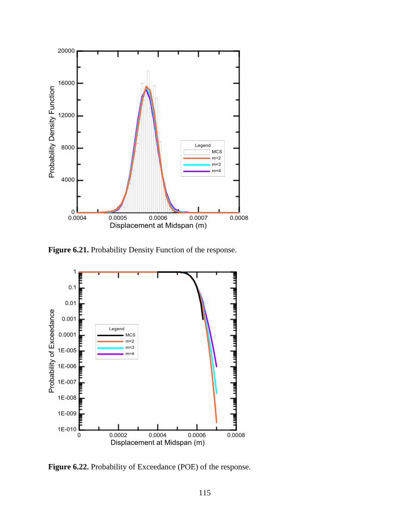
115
Figure 6.21. Probability Density Function of the response.
Figure 6.22. Probability of Exceedance (POE) of the response.

116
6.5.2.1 Computational Time
For the analysis of a concrete infinite beam on an elastic foundation, simulation of 1000 iterations
of the computer program takes 50 minutes on a personal computer with Intel I5-4690 4th
Generation Processor and 8GB of RAM. MDRM approximation based on 11 finite element
analyses takes 0.5 minutes and MaxEnt method requires 5.5 minutes. Thus, the total time taken by
MDRM is 6 minutes which is only 12% of the time taken by MCS.
6.5.3 Dynamic Continuum Problem
This problem will be solved considering that the elastic modulus of soil (𝐸𝑠) and the Poisson's
ratio (𝜇𝑠) are random variables using a Modified Vlasov Model as seen in Figure 6.16 (right).
The beam was considered to be 5 m in length, with a 10 kN dynamic load starting at the left side
and moving across the beam. 5 m of soil was considered on both sides of the beam. Table 6.28
defines each random variable used in this problem.
Table 6.28. Variables.
Variable Type of Distribution Parameters of Distribution
𝑬𝒔 Lognormal (20, 30%) – (mean, coefficient of variance)
𝝁𝒔 Lognormal (0.25, 7%) – (mean, coefficient of variance)
This problem was solved using Monte Carlo Simulation (MCS), and the Multiplicative
Dimensional Reduction Method (MDRM).
Using MCS, 1000 simulations were done for each random variable and each corresponding
displacement at the second node was calculated. Figure 6.23 shows the cumulative distribution of
the displacement at the second node. The mean and standard deviation were calculated as 0.001104
and 4.107E-05 respectively.

117
Figure 6.23. Cumulative distribution function of displacement at second node when load is at
initial position (m).
The MDRM was done using the fifth order (L=5) Gauss quadrature and considering two input
random variables (n=2). The Gauss Hermite formulas are adopted since the random variables
follow lognormal distribution. In total there are (2 × 5) + 1 = 11 response evaluations. For each
evaluation point, the other random variable is fixed to its mean value. Each response evaluation is
then substituted into the MATLAB computer program to determine the displacement at the second
node. MDRM approximation is used to calculate the statistical moment of the response function
(Table 6.29). This table also shows the relative errors between the statistical moments obtained by
MDRM and MCS which are very low showing a good agreement between the two methods.
Table 6.29. Statistical Moments of the response.
Displacement at
Node 2 (m)
MDRM (11 Trials) MCS (1000
Simulations)
Relative Error
(%)
First Moment 0.001103477 0.001103781 0.027511876
Second Moment 1.21934E-06 1.22002E-06 0.055696176
Standard Deviation 4.09579E-05 4.10703E-05 0.273797569
COV 0.037117088 0.037208753 0.246353469

118
Note: Relative Error (%) = |𝑀𝐶𝑆−𝑀𝐷𝑅𝑀|
𝑀𝐶𝑆× 100
The output responses obtained using MDRM are combined with the MaxEnt principle with
fractional moment constraints, in order to estimate the response probability distribution. Table 6.30
provides the Lagrange multipliers (𝜆𝑖) and the fractional exponents (𝛼𝑖) which are used to estimate
the probability distribution of the response. The number of fractional moments used are m=2, m=3,
and m=4.
Table 6.30. MaxEnt parameters for failure pressure.
Fractional
Moments
Entropy i 0 1 2 3 4
𝜆𝑖 700.5949 -2.61E+01 0.00050099
m=2 -8.6941 𝛼𝑖 -0.5321 -1.9365
𝑀𝑋𝛼𝑖 7.68E-12 3.29E-02
𝜆𝑖 493.8763 44.4784 -66.7168 1.21E-13
m=3 -8.6937 𝛼𝑖 0.6882 -0.3061 -4.8809
𝑀𝑋𝛼𝑖 5.14E-07 9.68E-01 7.16E+00
𝜆𝑖 700.5962 1010.034 1.81E+03 -2078.56 566.92
m=4 -8.6933 𝛼𝑖 0.9243 -0.6284 -0.6139 -0.3167
𝑀𝑋𝛼𝑖 3.16E-01 1.87E+01 1.15E-02 67.2909
The estimated probability distribution of the displacement at node 2 is compared to the MCS
(Figure 6.24). The probability distribution functions (PDF) using MDRM and MCS both matchup
accurately.
Then the probability of failure is estimated by plotting the probability of exceedance (POE) (Figure
6.25). The POE matches up very accurately. As the number of fractional moments increased, the
POE converged better and better to the MCS POE.

119
Figure 6.24. Probability Density Function of the response.
Figure 6.25. Probability of Exceedance (POE) of the response.

120
6.5.3.1 Computational Time
For the analysis of a concrete infinite beam on an elastic foundation, simulation of 1000 iterations
of the computer program takes 21 hours on a personal computer with Intel I5-4690 4th Generation
Processor and 8GB of RAM. MDRM approximation based on 11 finite element analyses takes
11.6 minutes and MaxEnt method requires 5.7 minutes. Thus the total time taken by MDRM is
17.5 minutes which is only 1.4% of the time taken by MCS.
6.5.4 Dynamic Discrete Problem
This problem will be solved considering that the compressive spring constant (𝑘𝑠) and the shear
parameter (𝑡𝑠) are random variables using a two parameter Pasternak Model as seen in Figure
6.15 (right). The beam was considered to be 10 m in length, with a 100 kN dynamic load starting
at the left side and moving across the beam. Soil was not considered on either side of the beam.
Table 6.31 defines each random variable used in this problem.
Table 6.31. Variables.
Variable Type of Distribution Parameters of Distribution
𝒌𝒔 Lognormal (1140000, 80%) – (mean, coefficient of variance)
𝒕𝒔 Lognormal (161993.8, 30%) – (mean, coefficient of variance)
The coefficient of variance (COV) of 𝑘𝑠 was increased significantly for this problem because when
a lower value of COV was used the program did not give final displacements that varied which in
turn did not give good results.
This problem was solved using Monte Carlo Simulation (MCS), and the Multiplicative
Dimensional Reduction Method (MDRM).
Using MCS, 1000 simulations were done for each random variable and each corresponding
midspan displacement was calculated when the load is at midspan. Figure 6.26 shows the
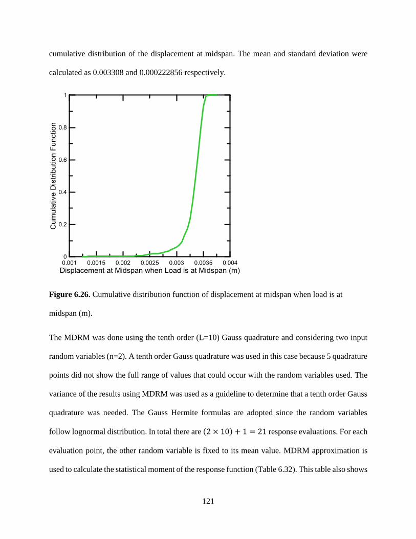
121
cumulative distribution of the displacement at midspan. The mean and standard deviation were
calculated as 0.003308 and 0.000222856 respectively.
Figure 6.26. Cumulative distribution function of displacement at midspan when load is at
midspan (m).
The MDRM was done using the tenth order (L=10) Gauss quadrature and considering two input
random variables (n=2). A tenth order Gauss quadrature was used in this case because 5 quadrature
points did not show the full range of values that could occur with the random variables used. The
variance of the results using MDRM was used as a guideline to determine that a tenth order Gauss
quadrature was needed. The Gauss Hermite formulas are adopted since the random variables
follow lognormal distribution. In total there are (2 × 10) + 1 = 21 response evaluations. For each
evaluation point, the other random variable is fixed to its mean value. MDRM approximation is
used to calculate the statistical moment of the response function (Table 6.32). This table also shows

122
the relative errors between the statistical moments obtained by MDRM and MCS which are very
low showing a good agreement between the two methods.
Table 6.32. Statistical Moments of the response.
Displacement at
Midspan (m)
MDRM (21 Trials) MCS (1000
Simulations)
Relative Error
(%)
First Moment 0.003317 0.003308 0.26254
Second Moment 1.10454E-05 1.0995E-05 0.458412477
Standard Deviation 0.000206204 0.000222856 7.472123149
COV 0.062164528 0.067361034 7.714409506
Note: Relative Error (%) = |𝑀𝐶𝑆−𝑀𝐷𝑅𝑀|
𝑀𝐶𝑆× 100
The output responses obtained using MDRM are combined with the MaxEnt principle with
fractional moment constraints, in order to estimate the response probability distribution. Table 6.33
provides the Lagrange multipliers (𝜆𝑖) and the fractional exponents (𝛼𝑖) which are used to estimate
the probability distribution of the response. The number of fractional moments used are m=2, m=3,
and m=4.
Table 6.33. MaxEnt parameters for failure pressure.
Fractional
Moments
Entropy i 0 1 2 3 4
𝜆𝑖 11.8013 -2.61E+14 3.91E+14
m=2 -7.2671 𝛼𝑖 4.575 4.6488
𝑀𝑋𝛼𝑖 1.35E-08 4.95E-08
𝜆𝑖 16.2638 -1.10E+11 5.25E+12 1.47E+13
m=3 -7.2374 𝛼𝑖 3.6044 4.344 4.8439
𝑀𝑋𝛼𝑖 1.10E-12 2.68E+02 1.02E-03
𝜆𝑖 111.9253 -7069.74 3.90E+09 8.48E+09 9.43E+09
m=4 -7.1064 𝛼𝑖 0.6768 3.8786 3.4294 3.9879
𝑀𝑋𝛼𝑖 2.10E-02 2.46E-10 3.19E-09 1.32E-10
The estimated probability distribution of the displacement at midspan is compared to the MCS
(Figure 6.27).

123
The probability distribution functions (PDF) do not match up that well. The MCS and MDRM
graphs start of the same but then due to the fact that 𝑘𝑠 does not affect the results as intended. In
fact this variable does not really affect the results at all which results in the poor results that were
achieved. Then the probability of failure is estimated by plotting the probability of exceedance
(POE) (Figure 6.28) which also shows a poor match between the two methods due to the same
reasoning as why the PDF plots did not match.
Figure 6.27. Probability Density Function of the response.

124
Figure 6.28. Probability of Exceedance (POE) of the response.
6.5.4.1 Computational Time
For the analysis of a concrete infinite beam on an elastic foundation, simulation of 1000 iterations
of the computer program takes 6.2 hours on a personal computer with Intel I5-4690 4th Generation
Processor and 8GB of RAM. MDRM approximation based on 21 finite element analyses takes 6.3
minutes and MaxEnt method requires 4.2 minutes. Thus the total time taken by MDRM is 10.5
minutes which is only 2.8% of the time taken by MCS.
6.6 Conclusions
Traditional reliability methods are very time consuming and often times make engineers not likely
to use them. This chapter studies the Multiplicative Dimensional Reduction Method in order show
that a reliability method exists that has the same accuracy of traditional methods while providing
much greater computational efficiency.

125
Through the last two examples in this paper the computationally efficiency of MDRM is on full
display. Without any drop in accuracy MDRM gives results much quicker (0.5% to 12% of time
taken to complete the problem using MCS) depending on the type of problem. The first two
examples showed that using MDRM with equations does not help. Instead MCS is more
computationally efficient when solving an equation based analysis, however the results between
MCS and MDRM are the same and the number of response evaluations using MDRM are
significantly less which helps when employing a finite element analysis. MDRM is especially
useful in the field of geomechanics as a lot of uncertainties exist. With most of the focus being on
finite element modelling and analyses, pairing it up with a reliability analysis using MDRM offers
great insight to engineers looking to design with the utmost respect to safety in mind.
126
7 Conclusions and Recommendations
7.1 Summary
Chapter 3 presented a model verification to ensure that the code developed to use the multiplicative
dimensional reduction method was implemented correctly. A simple example was done to compare
the results of MDRM, MCS and Cubature methods.
Chapter 4 presented two problems. The first problem was done considering all random variables
were not designated to be epistemic or aleatory. This problem was done using MDRM, Cubature
and MCS methods. It was determined that Cubature methods are not as accurate and required more
trials than MDRM therefore Cubature method was not used after this. The second problem was
done considering one random variable was epistemic and another was aleatory. This problem was
done using MDRM and MCS and the results were compared.
Chapter 5 presented a fire resistance problem. A performance based approach was explained and
used. This problem was done using MDRM and MCS and the results were compared.
Chapter 6 presented four geomechanics problems. The first set two problems were equation based
1D consolidation problems. The first problem was done to show a step by step method of how to
use MDRM. The results of MDRM were compared to MCS. The second problem was also done
using both MDRM and MCS and the results were compared. The second set of two problems were
finite element analyses. The first problem was of vertical drains. For this problem a finite element
model was created in ABAQUS and meshed. This mesh was then output into a FORTRAN code
provided by Dipanjan Basu. This problem was done using MDRM and MCS and the results were
compared. The second problem was of a concrete infinite beam on an elastic foundation. Two

127
foundation models were used (two parameter Pasternak Model and Modified Vlasov Model). Each
foundation model was done twice once for a static load and once for a dynamic load.
7.2 Conclusions
The main conclusion drawn from this research is that MDRM is efficient and it achieves accurate
results (compared to MCS) in a considerably less number of trials/simulations. In terms of equation
based problems MDRM is not worth implementing as MCS can be used and will lead to quicker
results. However, most analysis done in engineering is finite element analyses. This is when
MDRM provides considerable computational efficiency. Methods such as Cubature formulae were
also compared but did not offer the same amount of accuracy and efficiency as MDRM did.
Even when solving an equation based problem an incentive of using MDRM over MCS is that
MDRM provides the statistical moments, probability distribution, and if needed, the sensitivity
coefficients, which are related to the response of interest. MDRM paired with the maximum
entropy principle provides the probability distribution, therefore the probability of failure can be
calculated from that. Lastly, MDRM is very easy to be implemented but maybe not as easy for the
code to be developed. However, if a finite element analysis is to be done using a reliability method,
the time taken to develop a MDRM code is well worth it in order to get quick and precise answers
that cannot be had using other reliability methods.
7.3 Recommendations for Future Research
Future research can be extended more into the field of geomechanics and fire resistant design of
structures, considering a finite element analysis is done. Both these areas lack the use of reliability
analysis due to the high number of random variables and the stigma around traditional reliability
methods that tend to be computationally expensive. More problems done in these fields using

128
MDRM can lead to further use of reliability methods in these fields. Future research can also be
done for uncertainty problems with an epistemic variable. This paper covered an equation based
problem but a finite element analysis could be researched and that might make MDRM more useful
for an uncertainty problem with an epistemic variable.

129
References
Anderson, L. and Bergado, D. (1996). Soft ground improvement: In lowland and other
environments. New York, NY: American Society of Civil Engineers.
Bailey, C. (2006). Advances in fire engineering design of steel structures. Proceedings of the
Institution of Civil Engineers - Structures and Buildings, 159(1), pp.21-35.
Balasubramaniam, A., Alfaro, M. and Bergado, D. (1993). Improvement of soft Bangkok clay
using vertical drains. Geotextiles and Geomembranes, 12(7), pp.615-663.
Balomenos, G. (2015). Probabilistic Finite Element Analysis of Structures using the
Multiplicative Dimensional Reduction Method. PhD Thesis: University of Waterloo.
Basu, D. and Elhuni, H. (2017). Analytical Study for the Dynamic Response of Beams on
Pasternak Foundation. Proceedings of the 19th International Conference on Soil Mechanics and
Geotechnical Engineering, Seoul 2017.
Botev, Z., Taimre, T. and Kroese, D. (2011). Handbook of Monte Carlo methods. United States:
Wiley-Blackwell.
Christian, J. and Baecher, G. (2003). Reliability and statistics in Geotechnical engineering. New
York, NY, United States: John Wiley & Sons.
Cornell, A. and Benjamin, J. (1970). Probability, statistics and decisions for civil engineers. 7th
ed. New York: McGraw-Hill Inc.,US.
Ditlevsen, O. and Kiureghian, A. (2009). Aleatory or epistemic? Does it matter?. Structural
Safety, 31(2), pp.105-112.
Duan, X., Wang, M. and Kozluk, M. (2015). Acceptance criterion for probabilistic structural
integrity assessment: Prediction of the failure pressure of steam generator tubing with fretting
flaws. Nuclear Engineering and Design, 281, pp.154-162.
Ellingwood, B. (2005). Load combination requirements for fire-resistant structural design.
Journal of Fire Protection Engineering, 15(1), pp.43-61.
Girija Vallabhan, C. and Das, Y. (1991). Modified Vlasov Model for Beams on Elastic
Foundations. Journal of Geotechnical Engineering, 117(6), pp.956-966.
Guo, Q. and Jeffers, A. (2015). Finite-element reliability analysis of structures subjected to fire.
Journal of Structural Engineering, 141(4), p.
Hietaniemi, J. (2007). Probabilistic simulation of fire endurance of a wooden beam. Structural
Safety, 29(4), pp.322-336.

130
Holtz, R. (1987). Preloading with prefabricated vertical strip drains. Geotextiles and
Geomembranes, 6(1-3), pp.109-131.
Huang, P. and Delichatsios, M. (2010). Quantitative risk analysis for the response of steel beams
in fires. Journal of Structural Fire Engineering, 1(4), pp.231-241.
Iqbal, S. and Harichandran, R. (2010). Capacity reduction and fire load factors for design of steel
members exposed to fire. Journal of Structural Engineering, 136(12), pp.1554-1562.
Iqbal, S. and Harichandran, R. (2011). Capacity reduction and fire load factors for LRFD of steel
columns exposed to fire. Fire Safety Journal, 46(5), pp.234-242.
Isukapalli, S. (1999). Uncertainty Analysis of Transport-Transformation Models. PhD Thesis:
New Brunswick Rutgers, The State University of New Jersey.
Jaynes, E. (1957). Information theory and statistical mechanics. II. Physical Review, 108(2),
pp.171-190.
Jeffers, A., Jia, Z., Shi, K. and Guo, Q. (2012). Probabilistic evaluation of structural fire
resistance. Fire Technology, 49(3), pp.793-811.
Jensen, E., Van Horn, J. and Eamon, C. (2010). Variability of fire and concrete temperatures and
the associated uncertainty in structural behavior. Structures in Fire - Proceedings of the Sixth
International Conference, pp.959-966.
Jyrkama, M. and Pandey, M. (2016). On the separation of aleatory and epistemic uncertainties in
probabilistic assessments. Nuclear Engineering and Design, 303, pp.68-74.
Kozluk, M., Mills, B. and Pagan, S. (2006). Darlington steam generator tube fretting fitness-for-
service: operating experience and structural and leak-rate tests. Proceedings of the 5th CNS
International Steam Generator Conference.
Lange, D., Usmani, A. and Torero, j. (2008). The Reliability of Structures in Fire. Structures in
Fire - Proceedings of the Fifth International Conference, pp.760-770.
Lennox, W. and Kennedy, C. (2001). Moment operations on random variables, with applications
for probabilistic analysis. Probabilistic Engineering Mechanics, 16(3), pp.253-259.
Lind, N. and Hasofer, A. (1974). Exact and Invariant Second Moment Code Format. ASCE
Journal of the Engineering Mechanics Division, pp.111-121.
Lind, N., Krenk, S. and Madsen, H. (2006). Methods of structural safety. United States: Dover
Publications.
Loucks, D., Beek, E. and Stedinger, J. (2005). Water resources systems planning and
management. 1st ed. Paris: UNESCO.
131
Lu, J. and Darmofal, D. (2004). Higher-Dimensional Integration with Gaussian Weight for
Applications in Probabilistic Design. SIAM Journal on Scientific Computing, 26(2), pp.613-624.
Madhav, M., Prezzi, M. and Basu, D. (2009). Effect of soil disturbance on consolidation by
prefabricated vertical drains installed in a rectangular pattern. Geotechnical and Geological
Engineering, 28(1), pp.61-77.
Madsen, H. and Ditlevsen, O. (1996). Structural reliability methods. Chichester, United
Kingdom: Wiley, John & Sons.
Magnusson, S. and Pettersson, O. (1981). Rational design methodology for fire exposed load
bearing structures. Fire Safety Journal, 3(4), pp.227-241.
McNamee, J. and Stenger, F. (1967). Construction of fully symmetric numerical integration
formulas of fully symmetric numerical integration formulas. Numerische Mathematik, 10(4),
pp.327-344.
Melchers, R. (1987). Structural reliability: Analysis and prediction (Ellis Horwood series in civil
engineering). United Kingdom: Ellis Horwood Ltd , Publisher.
MIURA, N., PARK, Y. and MADHAV, M. (1993). Modelling and study of smear zones around
band shaped drains. SOILS AND FOUNDATIONS, 33(4), pp.135-147.
Mysovskikh, I. (1980). THE APPROXIMATION OF MULTIPLE INTEGRALS BY USING
INTERPOLATORY CUBATURE FORMULAE. Quantitative Approximation, pp.217-243.
Ono, T. and Zhao, Y. (2001). Moment methods for structural reliability. Structural Safety, 23(1),
pp.47-75.
Pandey, M., Walbridge, S. and Raimbault, J. (2015). Application of the Multiplicative
Dimensional Reduction Method (M-DRM) to a Probabilistic Fracture Mechanics Problem. 12th
International Conference on Applications of Statistics and Probability in Civil Engineering.
Phillips, G. (1980). A survey of one-dimensional and multidimensional numerical integration.
Computer Physics Communications, 20(1), pp.17-27.
Prezzi, M. and Basu, D. (2007). Effect of the smear and transition zones around prefabricated
vertical drains installed in a triangular pattern on the rate of soil consolidation. International
Journal of Geomechanics, 7(1), pp.34-43.
Rabitz, H., Rosenthal, C. and Li, G. (2001). High dimensional model representations. The
Journal of Physical Chemistry A, 105(33), pp.7765-7777.
Rahman, S. and Xu, H. (2004). A generalized dimension-reduction method for multidimensional
integration in stochastic mechanics. International Journal for Numerical Methods in
Engineering, 61(12), pp.1992-2019.

132
Rosenblueth, E. (1981). Two-point estimates in probabilities. Applied Mathematical Modelling,
5(5), pp.329-335.
Ryder, N., Wolin, S. and Milke, J. (2002). An investigation of the reduction in fire resistance of
steel columns caused by loss of spray-applied fire protection. Journal of Fire Protection
Engineering, 12(1), pp.31-44.
Sakji, S., Soize, C. and Heck, J. (2008). Probabilistic uncertainty modeling for
Thermomechanical analysis of Plasterboard submitted to fire load. Journal of Structural
Engineering, 134(10), pp.1611-1618.
Saouma, V. and Puatatsananon, W. (2006). Reliability analysis in fracture mechanics using the
first-order reliability method and Monte Carlo simulation. Fatigue Fracture of Engineering
Materials and Structures, 29(11), pp.959-975.
Schaferkotter, M. and Kythe, P. (2004). Handbook of computational methods for integration.
Boca Raton: Chapman & Hall/CRC.
Sobol, I. (1994). A Primer for the Monte Carlo method. Boca Raton, FL, United States: CRC
Press.
Stroud, A. (1966). Some Fifth Degree Integration Formulas for Symmetric Regions.
Mathematics of Computation, 20(93), p.90.
Stroud, A. and Secrest, D. (1963). Approximate Integration Formulas for Certain Spherically
Symmetric Regions. Mathematics of Computation, 17(82), p.105.
Sullivan, T. (2015). Introduction to uncertainty quantification: 2015. Switzerland: Springer
International Publishing AG.
Tagliani, A. and Novi Inverardi, P. (2003). Maximum entropy density estimation from fractional
moments. Communications in Statistics - Theory and Methods, 32(2), pp.327-345.
Taguchi, G. (1978). Performance analysis design. International Journal of Production Research,
16(6), pp.521-530.
Tang, W. and Ang, A. (1984). Probability: Concepts in engineering, planning and design: V. 2:
Decision, risk and reliability. New York: John Wiley and Sons (WIE).
Tang, W. and Ang, A. (2006). Probability concepts in engineering: Emphasis on applications to
civil and environmental engineering, Vol. 1. 2nd ed. New York, NY, United States: Wiley, John
& Sons.
Vaidogas, E. and Juocevičius, V. (2008). Reliability of a timber structure exposed to fire:
estimation using fragility function. Mechanika, 73, pp.35-42.

133
Van Coile, R., Annerel, E., Caspeele, R. and Taerwe, L. (2013). Full-probabilistic analysis of
concrete beams during fire. Journal of Structural Fire Engineering, 4(3), pp.165-174.
Victoir, N. (2004). Asymmetric Cubature Formulae with Few Points in High Dimension for
Symmetric Measures. SIAM Journal on Numerical Analysis, 42(1), pp.209-227.
Villanueva, D., Feijóo, A. and Pazos, J. (2013). Multivariate Weibull Distribution for Wind
Speed and Wind Power Behavior Assessment. Resources, 2(3), pp.370-384.
Wei, D., Cui, Z. and Chen, J. (2008). Uncertainty quantification using polynomial chaos
expansion with points of monomial cubature rules. Computers & Structures, 86(23-24), pp.2102-
2108.
Witteveen, J. and Twilt, L. (1981). A critical view on the results of standard fire resistance tests
on steel columns. Fire Safety Journal, 4(4), pp.259-270.
Wright, P., Wright, M., Reeds, J. and Lagarias, J. (1998). Convergence properties of the Nelder--
Mead Simplex method in low dimensions. SIAM Journal on Optimization, 9(1), pp.112-147.
Xu, H. and Rahman, S. (2004). A univariate dimension-reduction method for multi-dimensional
integration in stochastic mechanics. Probabilistic Engineering Mechanics, 19(4), pp.393-408.
Xu, J. and Lu, Z. (2017). Evaluation of Moments of Performance Functions Based on Efficient
Cubature Formulation. Journal of Engineering Mechanics, p.06017007.
Xu, J., Chen, J. and Li, J. (2012). Probability density evolution analysis of engineering structures
via cubature points. Computational Mechanics, 50(1), pp.135-156.
Zhang, K. and Li, G. (2010). A combined reliability analysis approach with dimension reduction
method and maximum entropy method. Structural and Multidisciplinary Optimization, 43(1),
pp.121-134.
Zhang, X. (2013). Efficient Computational Methods for Structural Reliability and Global
Sensitivity Analyses. PhD Thesis: University of Waterloo.
Zhang, X. and Pandey, M. (2013). Structural reliability analysis based on the concepts of
entropy, fractional moment and dimensional reduction method. Structural Safety, 43, pp.28-40.