reliability based assessment of quay walls
TRANSCRIPT
Reliability based Assessment
of Quay Walls
T.J. van der Wel

ii Thijs van der Wel | MSc thesis | Reliability based assessment of quay walls
iii Thijs van der Wel | MSc thesis | Reliability based assessment of quay walls
Reliability based Assessment of Quay
Walls
By
T.J van der Wel
in partial fulfilment of the requirements for the degree of
Master of Science
in Civil Engineering
at the Delft University of Technology,
to be defended publicly on 17 December 2018 at 1:00 PM
Graduation committee:
Prof. dr. ir. S.N. Jonkman TU Delft
Ir. P. Quist TU Delft / Witteveen+Bos
Dr. Ir. T. Schweckendiek TU Delft / Deltares
Ir. A.A. Roubos TU Delft / Havenbedrijf Rotterdam
Daily supervisor:
Ir. D.J. Jaspers Focks Witteveen+Bos
An electronic version of this thesis is available at http://repository.tudelft.nl/.

iv Thijs van der Wel | MSc thesis | Reliability based assessment of quay walls

v Thijs van der Wel | MSc thesis | Reliability based assessment of quay walls
ACKNOWLEDGMENTS
This thesis is the final work for my master program Hydraulic Engineering at Delft University of Technology.
The research concerns a reliability analysis of quay walls and was conducted at Witteveen+Bos, in agreement
with Port of Rotterdam and TU Delft.
First of all, I would like to thank Witteveen+Bos for providing me with the opportunity and all the facilities to
conduct this research. In particular, I am grateful to my two supervisors Peter Quist and Dirk-Jan Jaspers Focks.
Peter, thank you for your support and guidance throughout my entire research. I appreciate the positive
feedback you gave and your flexibility with regard to planning of meetings. Dirk-Jan, thanks for the fruitful
discussions we had and for sharing all your geotechnical knowledge. Additionally, I would like to thank all
other colleagues at Witteveen+Bos for their help and for making it a pleasant period.
Furthermore, words of thanks to all members of my graduation committee. I appreciate their advices and their
constructive feedback. It let me critically analyse my own work and helped me heading in the right direction.
Special thanks to Alfred Roubos, for sharing his experience and knowledge about probabilistic calculations of
quay walls. Also, I am grateful to Plaxis, and Dr. Ir. R. Brinkgreve in particular, for providing me with the newest
probabilistic module.
Finally, I would like to thank my friends and family for the grammar checking of my work and of course for all
their support during my entire study period at TU Delft.
Thijs van der Wel
Delft, December 2018

vi Thijs van der Wel | MSc thesis | Reliability based assessment of quay walls

vii Thijs van der Wel | MSc thesis | Reliability based assessment of quay walls
SUMMARY
Uncertainties in the soil parameters play a major role in the design of quay walls. In the current design
approach, partial factors are prescribed to account for uncertainties in the soil, as well as for other types of
uncertainties. This semi-probabilistic (level I) design approach needs to result in a reliable design for a range
of quay structures and for multiple soil stratifications. It is therefore expected that, in general, this method
results in overdimensioning of the structure. Whether this assumption holds, is investigated in this thesis by
carrying out a reliability analysis for two quay walls in the Port of Rotterdam.
Failure of a quay wall can be caused by plenty of different failure mechanisms. In this research, the failure
mechanisms yielding of the combi-wall, yielding of the anchor bar, shear failure of the grout body and soil
mechanical failure are assessed. Such failure mechanisms are complex soil-structure interaction problems.
Therefore, both the soil and the quay structure have been modelled with the finite element program Plaxis 2D,
using the Hardening soil model. For performing the probabilistic calculations on this model, the probabilistic
module ProbAna has been used. This is a package developed by Plaxis which couples several types of reliability
methods to the finite element software of Plaxis 2D. As the computational effort is relatively large with the
hardening soil model, the First Order Reliability Method (FORM) was used over sampling methods like
Directional Sampling and Crude Monte Carlo simulation.
The first case study concerned a combi-wall anchored by two grout anchors in the tubular steel piles of the
combi-wall. The results of the probabilistic calculations showed that the as-built quay wall has significant
overcapacity for all four failure mechanisms considered. This is in line with the expectations, but for the failure
mechanism yielding of the wall, it was also partly caused by the fact that the contractor had chosen to use
tubular piles with a larger wall thickness than originally required in the design.
Regarding the influence of variables, the calculations revealed that for the reliability of the anchor bar and the
combi-wall, the friction angle and the yield strength (both anchor and wall) were the most important
parameters. For the reliability of the grout body, it turned out that the pile class factor 𝛼𝑡 was most dominant.
For the purpose of deriving partial factors, the as-built design of the quay wall has been adjusted by reducing
the wall thickness of the tubular piles. In this way the design was more in line with the current design guidelines.
When comparing the derived partial factors with the prescribed partial factors of NEN9997, the general finding
is that slightly lower partial factors are found. The most important deviations were found for the friction angle
(a slightly lower partial factor was found) and the yield strength (a higher partial factor was found).
In the second case study a quay wall with relieving platform was considered. This quay wall is equipped with
monitoring sensors right from the construction. The available monitoring data for this quay wall is used for a
calibration of the Plaxis-model. Subsequently, the calibrated set of soil parameters was used as a starting point
for the probabilistic calculations. Two mechanism were evaluated for this quay wall, being yielding of the wall
and soil mechanical failure. For both limit states, the friction angle of the dense Pleistocene sand layer has
major influence on the reliability. It turned out that the obtained reliability indices are too low compared to
the target reliability. One of the explanations is that in the initial design, optimistic soil conditions were used,
especially for the Pleistocene sand layer, which might have resulted in a too optimistic design. Next to that,
the reliability is dominated by one single parameter, which can also result in a too low reliability index.
Although each case study concerned a different type of quay wall, the results reveal that choices made in the
design, either optimistic or pessimistic, can have large influence on the reliability. Perhaps just as important,
are the assumptions made regarding the stochastic description of the soil. It is still under discussion up to
what distance soil parameters are correlated in space and how spatial averaging should be applied. Reference
calculations showed that choices regarding the amount of independent soil layers and the degree of spatial
averaging have a large influence on the reliability. More fundamental research to these topics is therefore
recommended.
viii Thijs van der Wel | MSc thesis | Reliability based assessment of quay walls
LIST OF ABBREVIATIONS
AR Abdo-Rackwitz
CC Consequence Class
CMCS Crude Monte Carlo Simulation
COBYLA Constraint Optimization By Linear Approximation
CPT Cone Penetration Test
DS Directional Sampling
COV Coefficient Of Variation
CUR Civieltechnisch Centrum Uitvoering Research en Regelgeving
EC Eurocode
EMO Europees Massagoed Overslagbedrijf
FEM Finite Element Method
FORM First Order Reliability Method
GWL Ground water level
LLWS Low Low Water Spring
LSF Limit state Function
LSFE Limit State Function Evaluation(s)
MCS Monte Carlo Simulation
OWL Outer water level
PDF Probability Density Function
SLS Serviceability Limit State
ULS Ultimate Limit State
UC Unity check
RC Reliability Class
ix Thijs van der Wel | MSc thesis | Reliability based assessment of quay walls
LIST OF SYMBOLS
Reliability symbols
𝛼 Sensitivity factor [-]
𝛽 Reliability index [-]
𝜇 Mean [-]
𝜎 Standard deviation [-]
𝛾 Partial factor [-]
𝑃𝑓 Failure probability [-]
𝑋𝑘 Characteristic value / Representative value [-]
𝑋𝑑 Design value [-]
𝑋𝑖 Random variable of vector 𝑋 [-]
𝑋∗ Design point in FORM [-]
𝑍 Limit state function [-]
Geotechnical symbols
𝛼𝑡 Pile class factor [-]
𝑐 Cohesion [kPa]
𝛾𝑢𝑛𝑠𝑎𝑡 Unsaturated volumetric weight [kN/m3]
𝛾𝑠𝑎𝑡 Saturated volumetric weight [kN/m3]
𝜏 Shear stress [kPa]
𝜑’ Friction angle [°]
Ψ Dilatancy angle [°]
𝛿 Wall friction angle [°]
𝐸𝑜𝑒𝑑𝑟𝑒𝑓
Oedometer stiffness [kN/m2]
𝐸50𝑟𝑒𝑓
Secant stiffness [kN/m2]
𝐸𝑢𝑟𝑟𝑒𝑓
Unloading / Reloading stiffness [kN/m2]
𝐾0𝑛𝑐 Neutral lateral earth pressure coefficient for non-consolidated soil [-]
𝐾𝑎 Active lateral earth pressure coefficient [-]
𝐾𝑝 Passive lateral earth pressure coefficient [-]
𝑚 Power in stress-dependent stiffness relation [-]
𝑀𝑠𝑓 Safety factor from a phi-c reduction in Plaxis [-]
𝑞𝑐 Cone resistance [MPa]
𝑅𝑖𝑛𝑡𝑒𝑟 Interface strength ratio [-]
Structural properties
𝐴 Area [m2]
𝐷𝑡𝑢𝑏𝑒 Diameter tubular pile [m]
𝐸 Youngs’ modulus [kN/m2]
𝑓𝑦 Yield strength [N/mm2]
𝑀 Moment force [kNm]
𝑁 Normal force [kN]
𝑂 Circumference [m]
𝑡𝑡𝑢𝑏𝑒 Wall thickness tubular pile [m]
𝑊𝑒𝑙 Elastic section modulus [m3]

x Thijs van der Wel | MSc thesis | Reliability based assessment of quay walls
TABLE OF CONTENTS
ACKNOWLEDGMENTS V
SUMMARY VII
LIST OF ABBREVIATIONS VIII
LIST OF SYMBOLS IX
1 INTRODUCTION 1
1.1 Background 1
1.1 Problem definition 1
1.2 Objective and research questions 2
1.3 Thesis outline 2
2 THEORETICAL BACKGROUND 4
2.1 Quay walls 4
2.1.1 History of quay walls in Rotterdam 4 2.1.2 Functions of a quay wall 5 2.1.3 The Rotterdam quay wall 6
2.2 Soil mechanics related to quay walls 9
2.2.1 Lateral earth pressure 9 2.2.2 Working of a relieving platform 10
2.3 Modelling of soil and structure 12
2.3.1 Soil models 12 2.3.2 Limitations 12
2.5 Uncertainty and reliability 15
2.5.1 Sources of uncertainty in Civil Engineering 15 2.5.2 Safety philosophy 16
2.6 Design methods 17
2.6.1 Level IV 17 2.6.2 Level III 17 2.6.3 Level II 19 2.6.4 Level I 21 2.6.5 Level 0 23
2.7 Design guidelines for quay walls 24
2.7.1 CUR 166 Sheet pile structures 24 2.7.2 CUR 211 Quay walls 24 2.7.3 Probabilistic background of the CUR211 24

xi Thijs van der Wel | MSc thesis | Reliability based assessment of quay walls
2.8 Conclusion 27
3 METHOD DESCRIPTION 28
3.1 Selection of Failure Mechanisms 29
3.2 Limit State Functions 31
3.2.1 Failure of combi-wall profile 31 3.2.2 Anchor rod failure 33 3.2.3 Soil mechanical failure 34
3.3 Coupling of FEM with Reliability Analysis Methods 36
3.3.1 Main findings in previous research on coupling Reliability Analysis Methods
with Plaxis 36 3.3.2 Overall conclusion 38 3.3.3 Functionality of ProbAna 38 3.3.4 Selection of FORM algorithm 40
4 STARTING POINTS 41
4.1 Introduction 41
4.2 Soil parameter uncertainties 42
4.3 Structural parameters 45
4.4 Geometrical parameters 47
4.5 Load parameters 48
5 CASE STUDY 1: DOUBLE ANCHORED COMBI-WALL 49
5.1 Introduction 49
5.2 Starting points 50
5.2.1 Soil parameters 50 5.2.2 Structural parameters 52 5.2.3 Construction stages and meshing 53 5.2.4 Loads, water levels and geometry 53
5.3 LS1: Yielding of the combi-wall 54
5.3.1 FORM sensitivity analysis 56 5.3.2 FORM with correlated parameters 57 5.3.3 Run with characteristic yield strength 59 5.3.4 Influence of time-dependent loads 62 5.3.5 Validation of Abdo-Rackwitz algorithm 63 5.3.6 Redesign of the retaining wall 64 5.3.7 First conclusions 65
5.4 LS2: Yielding of the anchor rod 66
5.5 LS3: Soil mechanical failure 68
5.6 Intermediate conclusion 71
5.6.1 Reliability of the structure 71
xii Thijs van der Wel | MSc thesis | Reliability based assessment of quay walls
5.6.2 Plaxis-FORM coupling (ProbAna) 71
5.7 LS4: Shear resistance of anchorage inadequate 73
5.8 Derivation of partial factors 78
5.8.1 Approach 78 5.8.2 LS1: Yielding of the wall 79 5.8.3 LS2: Yielding of the anchor bar 81 5.8.4 LS3: Soil mechanical failure 81 5.8.5 Differentiation between Reliability Classes 82 5.8.6 Overall conclusion partial factors 83
6 CASE STUDY 2: QUAY WALL WITH RELIEVING PLATFORM 85
6.1 General description of the structure 85
6.2 Description of the measurement program 87
6.3 Approach for calibration and reliability analysis 89
6.4 Calibration of the model 91
6.4.1 Measured displacements versus calculated displacements 92
6.5 Probabilistic calculations 94
6.5.1 Starting points 94 6.5.2 LS1: Soil mechanical failure 94 6.5.3 LS2: Yielding of the combi-wall 96
7 DISCUSSION 98
7.1 Influence of soil stratification 98
7.2 Influence of the stochastic description of soil parameters 98
7.3 Extreme values for soil parameters in FORM design points 100
7.4 Influence of the use of monitoring data on the reliability 101
7.5 Wider applicability of the results of both case studies 102
8 CONCLUSIONS AND RECOMMENDATIONS 103
8.1 Conclusions 103
8.2 Recommendations 106
REFERENCES 108
Last page 110
APPENDICES
A Fault tree for CUR211, first edition 113
B Performance of algorithms OpenTURNS 115
C Monte Carlo Simulation for Structural properties combi-wall 120
D Fault tree simple quay wall 124

xiii Thijs van der Wel | MSc thesis | Reliability based assessment of quay walls
E Plaxis output results simple quay wall 126
F FORM output simple quay wall 129
G FORM output for deriving partial factors 131
H Plaxis soil models 133
I Soil profile EMO 136
J FORM output EMO quay wall 140
K FORM output EMO quay wall for non-calibrated design 142


1 Thijs van der Wel | MSc thesis | Reliability based assessment of quay walls
1
INTRODUCTION
1.1 Background
In the Netherlands thousands of kilometres of quay walls have been built. These quay walls are used for all
kinds of purposes. You can think for example of quay walls in city centres and quay walls in port areas. Although
we have gained a lot of experience and knowledge over the years regarding the design and construction of
these type of structures, still a lot of topics remain not fully understood. One of the main challenges lies in the
description and modelling of the soil and its interaction with the structure. Of course, with local soil
investigation useful information regarding soil stratification and soil properties is gathered. However it does
not provide specific information regarding the soil-structure interaction. Uncertainties in the soil properties
arise due to several causes:
· Spatial variability of soil properties
· Sample disturbance in laboratory tests
· Imprecision of in-situ testing methods
· Imprecision and differences in laboratory tests and equipment
For the design of quay walls the engineer has to account for all the uncertainties. Apart from uncertainties in
the description of the soil also other aspects are uncertain, think of the uncertainty in the use of the quay walls
during their lifetime or the lack of knowledge to describe reality with a model. These uncertainties have to be
accounted for to guarantee a reliable design. To quantify reliability, it is coupled to the probability of failure
of a structure. In design guidelines, the reliability of a quay wall is expressed in a reliability index (β), which is
directly related to the probability of failure. Based on the consequences of failure, a specific value for the
reliability index, the target reliability, is prescribed. Structures with high economical and societal risk require a
higher degree of safety than structures with minimal consequences in case of failure.
Current design guidelines make use of a semi-probabilistic method (Level I) to reach the prescribed target
reliability. This method makes use of partial safety factors to account for the uncertainty in the model, the load
and the resistance. The magnitude of these factors is either based on experience gathered in large amount of
completed projects or calibration with a probabilistic analysis (Level II or level III). As guidelines should be
applicable to a certain range of similar structures, the partial factors should guarantee the safety in all of these
cases. This can result in conservative values of the partial factors and respectively ‘over-design’ of the structure.
1.1 Problem definition
The main reasons why almost all quay walls are designed using a semi-probabilistic method instead of a full
probabilistic analysis are the lack of statistical data, the complexity of a full probabilistic method and the time
it takes to perform such an analysis.
Calibration studies regarding partial factors for quay walls, mostly in the Port of Rotterdam, have been
performed in the past by Huijzer (1996), de Grave (2002), Havinga (2004) and Wolters (2012). However
probabilistic calculations with more advanced soil models, like the Plaxis Hardening Soil model, for quay walls
with relieving platform has only been performed by Wolters. Therefore it is still a relatively open field of
research. Thus, it is uncertain whether the semi-probabilistic design method results in the required level of
safety. It is possible that quay walls have more capacity than expected and thus are safer, which would allow
heavier loading of the quay wall or alternatively a cheaper design. On the other hand quay walls might turn
out less safe than expected.
2 Thijs van der Wel | MSc thesis | Reliability based assessment of quay walls
To get better insight into this question, multiple quay walls within the Port of Rotterdam have been equipped
with sensors to measure e.g. water levels, anchor forces and displacements, resulting in monitoring data of
many years. This data provides useful information about how well a model predicts the actual behaviour of a
quay wall
1.2 Objective and research questions
The main questions described in the problem definition is whether the use of a semi-probabilistic design
approach for quay walls results in the required level of safety and the most cost-efficient design. This can be
investigated by performing a full probabilistic analysis in which the uncertainties in the load and resistance
parameters are taken into account. The objective of this research is threefold:
1 Establishing the actual reliability index of a quay wall in operation
2 Exploring possibilities for an increase in retaining height making use of probabilistic calculations
3 Verifying the partial factors of the current design guidelines
The term actual refers here to the as-built design of the structure and the more or less known loading
conditions. The availability of monitoring data for the quay wall with relieving platform considered in this
research allows for a calibration of the Plaxis-model, which subsequently will be used as a starting point for
the probabilistic calculations.
The following sub questions will help to reach the above described objectives:
1 What are the most suitable probabilistic methods to determine the reliability of a quay wall modelled
with FEM?
2 What are the most sensitive parameters for each failure mode and for the overall system reliability?
3 How can monitoring data be used for model calibration and parameter distribution updating ?
4 How can this research contribute to an improvement of the current design guidelines?
Answers to these questions will be gathered in this thesis in order to contribute to the main objectives.
1.3 Thesis outline
This subchapter describes the outlines of the report. Starting with Chapter 1, in which the problem is defined
and the main objective of the thesis is described.
Chapter 2 covers a summary of the performed literature study. First the history of quay walls in Rotterdam has
been described together with the main functions and components of a quay wall. The knowledge about the
most relevant soil mechanics is summarized. Thereafter, the different types of uncertainty that play a role in
the design or assessment of a structure are defined. Then, the concept of safety and the different design
methods to account for uncertainty are described. This knowledge is helpful to understand the background of
the relevant codes and guidelines for the design of quay walls, which are elaborated at the end of the chapter.
In Chapter 3 the methodology of the research is given. First, a more thorough analysis in the system reliability
of a quay wall will be performed. The fault tree presented in Chapter 2 will be discussed and it will be decided
which failure mechanisms will be assessed and which one will be left out of this research. For each failure
mechanism the limit state function will be formulated and the appropriate probabilistic method should be
chosen to perform the limit state evaluations based on a consideration of computational effort, accuracy and
stability. Thereafter the coupling between a FEM and a reliability analysis by using ProbAna is explained.
In chapter 4 the starting points for the two considered case studies are defined. Already many research has
been done into the statistical distributions and correlations between parameters. Therefore, to safe time, the
determination of the parameters will be mainly based on the findings in previous research.
Chapter 5 is devoted to the first case study, in which a simple quay wall is handled. First, the quay structure is
described together with all the assumptions made. Thereafter, the reliability index for four mechanisms have

3 Thijs van der Wel | MSc thesis | Reliability based assessment of quay walls
been determined for the as-built structure. In the end of this chapter, a new set of partial factors is derived
based on the outcomes of the probabilistic calculations. These partial factors are compared with the current
prescribed factors and their validity has been discussed.
Chapter 6 covers the case study about a quay wall with relieving platform. At first, the structure is described
together with the monitoring program for this quay wall. Following, the calibration of the model using the
monitoring data is treated. Thereafter, for two critical limit states the failure probability is determined.
In chapter 7 the obtained results of the research are discussed. The influence on the reliability of changing the
soil stratification and the stochastic description of soil parameters is investigated. Also the influence of the use
of monitoring data with respect to the reliability is investigated.
To end, in chapter 8, the conclusions and recommendations will be given.

4 Thijs van der Wel | MSc thesis | Reliability based assessment of quay walls
2
THEORETICAL BACKGROUND
In this chapter the existing knowledge about quay walls, uncertainties and reliability is described. The chapter
is predominantly focussed on quay walls in the region of the Port of Rotterdam. In the first subchapter the
focus is on the structure itself, while the second subchapter is devoted to the soil behaviour and interaction of
the soil with the quay wall structure. Thereafter the different sources of uncertainty are treated together with
design methods to account for these uncertainties.
2.1 Quay walls
To get a better understanding of the choices made in the design of quay walls, the development of the quay
walls in Rotterdam is analysed by considering its history, functions and structural elements.
2.1.1 History of quay walls in Rotterdam
The easiest method to transport large amounts of heavy goods has always been over water as it requires
relatively seen the least amount of energy. The oldest sea trade is dated from already 6000 years ago in the
region of Egypt, where they transported cargo like grains and cattle over sea. It was not before the seventeenth
century the Port of Rotterdam really started to develop. In the city centre of Rotterdam the first quays were
constructed to accommodate fishing boats. In the late 19th century, with the start of the industrial revolution
in the Netherlands, the port started to develop rapidly, see Figure 2.1. The introduction of new materials like
steel and the introduction of ship engines had a large impact on the vessel size and therefore on the draught
of the vessel.
Figure 2.1 Rotterdam’s port development. Source: Port of Rotterdam (n.d.)
This required larger water depths and therefore the port started to grow in the direction of the sea, where
larger depths were available. The increase in retaining height of quay walls also resulted in changes in the
design. Due to the soft clay and peat deposits in Rotterdam, gravity type structures were losing popularity

5 Thijs van der Wel | MSc thesis | Reliability based assessment of quay walls
because of the expensive soil improvements that were required. Therefore quay walls on foundation piles were
introduced in the period around 1930 to cope with this problem, see Figure 2.2.
Figure 2.2 Cross section of a quay wall in Rotterdam, 1930, Source: de Gijt (2010)
After the Second World War, in which large parts of the port were destroyed, the Port of Rotterdam was quickly
rebuilt and started to grow to a port of world size. Especially the handling of dry bulk, liquid bulk and
containerized goods contributed to the growth up to the largest port in the world in 1962. The continuous
increase in retaining height, crane size and surcharge load resulted in further adaption of the quay wall
structures. A more or less typical quay structure was arising in PoR, shown in Figure 2.3. This typical “Rotterdam
quay wall” will be further described in the remainder of this chapter.
Figure 2.3 Cross-section of the Euromax terminal in Rotterdam, 2007. Source: de Gijt (2010)
2.1.2 Functions of a quay wall
Before going more in depth into the composition of the quay wall, first the main functions will be elaborated
for a better understanding of the relevance of the different components. The main functions a quay wall can
explained on the hand of Figure 2.3.
· Retaining function
As depicted, the quay wall creates a clear separation between soil and water. Without the quay wall it
would not be possible to create a step in surface level of 26,5m. The result of this sharp separation is
a large horizontal load of the soil body to be retained by the quay structure. Another important aspect
is the water retaining function. As ports are often in coastal zones, the port can be part of a flood
protection system. With a sufficient height of the surface level, a flood will not be able to reach the
hinterland.
· Mooring function
The container vessel that is depicted is moored nicely along the quay. However, this is not so self-
evident as it seems. The vessels position is influenced by hydraulic conditions like currents, waves and

6 Thijs van der Wel | MSc thesis | Reliability based assessment of quay walls
wind, whereas for safe container handling, the vessel is not allowed to move significantly. By mooring
of the vessel, the hydraulic loads on the vessel are transferred via the mooring lines and the bollards
to the quay structure, making container handling or other ship to shore activities possible.
· Protection function
Before the vessel is moored along the quay, a whole operation of approaching the quay, called
berthing, is already behind. With a large vessel and expensive quay structure it should be prevented
that one of the two get damaged. This is realised by the installation of fenders and berthing dolphins.
Fenders are (often) steel objects attached to the side of the quay wall. When the vessels is approaching
the quay, the hull of the vessel is pushing against the fender. The fender is relatively elastic in
comparison with the concrete top structure of the quay and deforms during the berthing process. With
this deformation, the kinetic energy of the vessel is adopted by the fender, leaving the quay and the
vessel undamaged. The force in the fender is transferred to the quay though and have to be further
transferred to the soil.
· Bearing function
On the land side of the quay wall, port operations like loading and unloading of the vessel and storage
of goods close to quay are ongoing. This results in mainly vertical loads imposed on the quay structure
and the adjacent soil body. The quay wall must be able to bear the imposed loads to guarantee safe
and secure port operations.
2.1.3 The Rotterdam quay wall
Although several solutions are available for the design of a quay wall, most of the quay walls in Rotterdam
show a similar type of design. To be able to explain this, the different type of retaining structures are considered
together with their applicability in the Port of Rotterdam:
· Gravity structures (Picture A of Figure 2.4)
The main principle of this type of structure is to use the weight of the structure to create sufficient
friction between soil and structure to resist the lateral loads.
· Sheet pile structures (Picture B)
Sheet pile structures creates a balance between horizontal loads by their extra embedded depth and/or
installed anchors
· Piled structures (Picture C)
Piled structures are basically a concrete deck element supported by vertical or raked piles. This type of
structure allows for an open structure where the water can flow underneath the top element
· Combinations of the above mentioned types
A) Gravity structure B) Sheet pile structure C) Piled structure
Figure 2.4 Different types of quay wall structures. Source: de Gijt (2010)
For the design of a quay wall the designer has to make a decision on which type to use. This decision is
influenced by many factors, of which the most important are:
· geological conditions
· retaining height
· loading on the structure
· constructability
7 Thijs van der Wel | MSc thesis | Reliability based assessment of quay walls
Due to the heavy weight of gravity type structures, a significant load on the subsoil is imposed and therefore
good subsoil conditions are required. In Rotterdam the subsoil consists of several very weak layers of peat and
clay making soil improvements a prerequisite for this type of structures. Besides, all vertical loads and the
moment generated by the horizontal loads have to be taken by only compressive stresses in the subsoil, which
can cause problems in case of large retaining heights.
Sheet pile structures are a more convenient solution in case of weak soil conditions. Especially with the use of
anchors to reduce the horizontal load on the sheet pile, this system is cheap and relatively easy to construct.
However, in case of large retaining heights (>15m) and heavy surcharge loads problems start to arise with
respect to constructability, bending moment resistance and vertical bearing capacity of sheet piles. The
driveability of sheet piles is limited to approximately 30-35m, after which the chance of interlocking failure and
damage to sheet piles considerably increases. This problem, together with the other two, can be partly solved
by the use of combi-walls. This is a combination of steel tubular piles with sheet pile elements in between. The
tubular piles take the main loads in this system, whereas the sheet pile elements function as retention for soil
and water. For retaining heights larger than 20m, this system reaches its limits as well.
Piled systems are a suitable solution as well in case of soft soil deposits. Large surcharge loads can be easily
transferred to the subsoil with this system. The horizontal resistance of a pile system is limited though and
thus a system that combines the benefits of both a piled system and a sheet pile system have arisen in the
Port of Rotterdam (Figure 2.5).
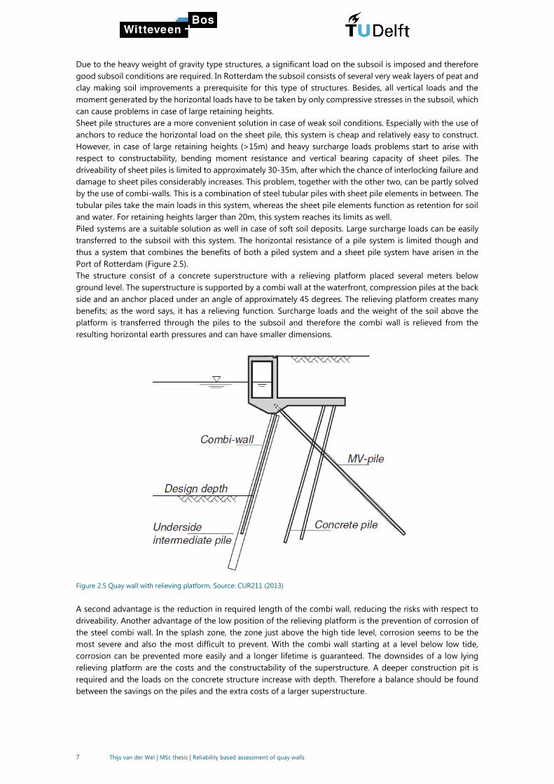
The structure consist of a concrete superstructure with a relieving platform placed several meters below
ground level. The superstructure is supported by a combi wall at the waterfront, compression piles at the back
side and an anchor placed under an angle of approximately 45 degrees. The relieving platform creates many
benefits; as the word says, it has a relieving function. Surcharge loads and the weight of the soil above the
platform is transferred through the piles to the subsoil and therefore the combi wall is relieved from the
resulting horizontal earth pressures and can have smaller dimensions.
Figure 2.5 Quay wall with relieving platform. Source: CUR211 (2013)
A second advantage is the reduction in required length of the combi wall, reducing the risks with respect to
driveability. Another advantage of the low position of the relieving platform is the prevention of corrosion of
the steel combi wall. In the splash zone, the zone just above the high tide level, corrosion seems to be the
most severe and also the most difficult to prevent. With the combi wall starting at a level below low tide,
corrosion can be prevented more easily and a longer lifetime is guaranteed. The downsides of a low lying
relieving platform are the costs and the constructability of the superstructure. A deeper construction pit is
required and the loads on the concrete structure increase with depth. Therefore a balance should be found
between the savings on the piles and the extra costs of a larger superstructure.

8 Thijs van der Wel | MSc thesis | Reliability based assessment of quay walls
Both the combi wall and the compression piles are placed under an angle. In this way, the piles can take up
lateral loads on the superstructure in their axial direction as well, reducing the horizontal load on the anchors
and the combi wall. The combi wall is often placed directly under the crane rail track of the of the quay, so that
crane loads can directly be transferred to the combi wall without inducing large bending moments in the
superstructure.
These main design principles can be recognized in most quay walls with a large retaining heights in Rotterdam.
Client specific requirements and local boundary conditions make that quay walls still deviate at certain aspects
from one to another.
9 Thijs van der Wel | MSc thesis | Reliability based assessment of quay walls
2.2 Soil mechanics related to quay walls
The main load on a quay wall as well as the resistance of the quay wall is provided by the surrounding soil.
Therefore the soil mechanics that play a role in the design of a quay wall are discussed in this subchapter.
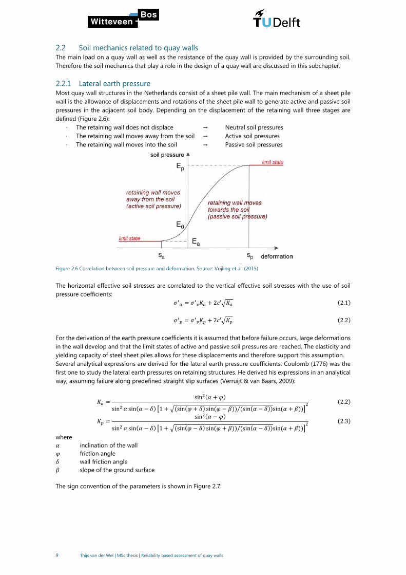
2.2.1 Lateral earth pressure
Most quay wall structures in the Netherlands consist of a sheet pile wall. The main mechanism of a sheet pile
wall is the allowance of displacements and rotations of the sheet pile wall to generate active and passive soil
pressures in the adjacent soil body. Depending on the displacement of the retaining wall three stages are
defined (Figure 2.6):
· The retaining wall does not displace → Neutral soil pressures
· The retaining wall moves away from the soil → Active soil pressures
· The retaining wall moves into the soil → Passive soil pressures
Figure 2.6 Correlation between soil pressure and deformation. Source: Vrijling et al. (2015)
The horizontal effective soil stresses are correlated to the vertical effective soil stresses with the use of soil
pressure coefficients:
𝜎′𝑎 = 𝜎′𝑣𝐾𝑎 + 2𝑐′√𝐾𝑎 (2.1)
𝜎′𝑝 = 𝜎′𝑣𝐾𝑝 + 2𝑐′√𝐾𝑝 (2.2)
For the derivation of the earth pressure coefficients it is assumed that before failure occurs, large deformations
in the wall develop and that the limit states of active and passive soil pressures are reached. The elasticity and
yielding capacity of steel sheet piles allows for these displacements and therefore support this assumption.
Several analytical expressions are derived for the lateral earth pressure coefficients. Coulomb (1776) was the
first one to study the lateral earth pressures on retaining structures. He derived his expressions in an analytical
way, assuming failure along predefined straight slip surfaces (Verruijt & van Baars, 2009):
𝐾𝑎 =sin2(𝛼 + 𝜑)
sin2 𝛼 sin(𝛼 − 𝛿) [1 + √(sin(𝜑 + 𝛿) sin(𝜑 − 𝛽))/(sin(𝛼 − 𝛿))sin(𝛼 + 𝛽))]2
(2.2)
𝐾𝑝 =sin2(𝛼 − 𝜑)
sin2 𝛼 sin(𝛼 − 𝛿) [1 + √(sin(𝜑 − 𝛿) sin(𝜑 + 𝛽))/(sin(𝛼 − 𝛿))sin(𝛼 + 𝛽))]2
(2.3)
where
𝛼 inclination of the wall
𝜑 friction angle
𝛿 wall friction angle
𝛽 slope of the ground surface
The sign convention of the parameters is shown in Figure 2.7.
10 Thijs van der Wel | MSc thesis | Reliability based assessment of quay walls
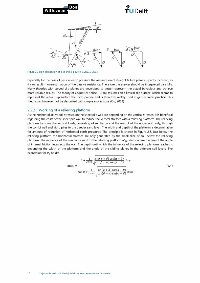
Figure 2.7 Sign convention of β, α and δ. Source: CUR211 (2013)
Especially for the case of passive earth pressure the assumption of straight failure planes is partly incorrect, as
it can result in overestimation of the passive resistance. Therefore the answer should be interpreted carefully.
Many theories with curved slip planes are developed to better represent the actual behaviour and achieve
more reliable results. The theory of Caquot & Kerisel (1948) assumes an elliptical slip surface, which seems to
represent the actual slip surface the most precise and is therefore widely used in geotechnical practice. This
theory can however not be described with simple expressions (Ou, 2013)
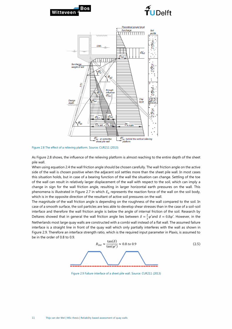
2.2.2 Working of a relieving platform
As the horizontal active soil stresses on the sheet pile wall are depending on the vertical stresses, it is beneficial
regarding the costs of the sheet pile wall to reduce the vertical stresses with a relieving platform. The relieving
platform transfers the vertical loads, consisting of surcharge and the weight of the upper soil body, through
the combi wall and vibro piles to the deeper sand layer. The width and depth of the platform is determinative
for amount of reduction of horizontal earth pressures. The principle is shown in Figure 2.8. Just below the
relieving platform the horizontal stresses are only generated by the small slice of soil below the relieving
platform. The influence of the surcharge next to the relieving platform 𝜎′𝑘0 starts where the line of the angle
of internal friction intersects the wall. The depth until which the influence of the relieving platform reaches is
depending the width of the platform and the angle of the sliding planes in the different soil layers. The
expression for 𝜃𝑎 holds:
tan 𝜃𝑎 =
1 +1
𝑐𝑜𝑠𝛼√sin(𝜑 + 𝛿) cos(𝛼 + 𝛽)cos(𝛿 − 𝛼) sin(𝜑 − 𝛽)
𝑠𝑖𝑛𝜑
tan 𝛼 +1
𝑐𝑜𝑠𝛼√sin(𝜑 + 𝛿) cos(𝛼 + 𝛽)cos(𝛿 − 𝛼) sin(𝜑 − 𝛽)
𝑐𝑜𝑠𝜑
(2.4)
11 Thijs van der Wel | MSc thesis | Reliability based assessment of quay walls
Figure 2.8 The effect of a relieving platform. Source; CUR211 (2013)
As Figure 2.8 shows, the influence of the relieving platform is almost reaching to the entire depth of the sheet
pile wall.
When using equation 2.4 the wall friction angle should be chosen carefully. The wall friction angle on the active
side of the wall is chosen positive when the adjacent soil settles more than the sheet pile wall. In most cases
this situation holds, but in case of a bearing function of the wall the situation can change. Settling of the toe
of the wall can result in relatively larger displacement of the wall with respect to the soil, which can imply a
change in sign for the wall friction angle, resulting in larger horizontal earth pressures on the wall. This
phenomena is illustrated in Figure 2.7 in which 𝐸𝑎 represents the reaction force of the wall on the soil body,
which is in the opposite direction of the resultant of active soil pressures on the wall.
The magnitude of the wall friction angle is depending on the roughness of the wall compared to the soil. In
case of a smooth surface, the soil particles are less able to develop shear stresses than in the case of a soil-soil
interface and therefore the wall friction angle is below the angle of internal friction of the soil. Research by
Deltares showed that in general the wall friction angle lies between 𝛿 =2
3𝜑′and 𝛿 = 0.8𝜑′. However, in the
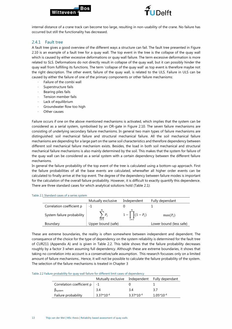
Netherlands most large quay walls are constructed with a combi wall instead of a flat wall. The assumed failure
interface is a straight line in front of the quay wall which only partially interferes with the wall as shown in
Figure 2.9. Therefore an interface strength ratio, which is the required input parameter in Plaxis, is assumed to
be in the order of 0.8 to 0.9.
𝑅𝑖𝑛𝑡 ≈tan(𝛿)
tan(𝜑′)≈ 0.8𝑡𝑜0.9 (2.5)
Figure 2.9 Failure interface of a sheet pile wall. Source: CUR211 (2013)

12 Thijs van der Wel | MSc thesis | Reliability based assessment of quay walls
2.3 Modelling of soil and structure
The shape of a quay wall and the behaviour of soil are often too complex to describe with simple analytical
equations, whereas advanced equations e.g. partial differential equations become too complex to solve
analytically. Besides, the soil-structure interaction can hardly be described with analytical equations. This can
result in inaccurate outcomes in (geo)technical calculations of e.g. forces and displacements.
With the development of the Finite Element Method the soil and the structure are described in a more
fundamental way. Finite Element refers to the fact a structure is divided in a finite number of small elements.
These elements are all interconnected by nodes. The partial differential equations that describe the constitutive
relations, are discretized and approximated in the nodes. Together with the boundary conditions in the nodes,
the set of equations is solved using matrix computations. This finally results in displacements and stresses for
the entire considered structure.
The number of nodes, or the mesh size, determines for a large part the accuracy of the calculations. A finer
mesh leads to more accurate results but the downside is the increase in computational time.
The most commonly used FEM-software to model soil-related problems in the Netherlands is Plaxis. This
software package is thus used throughout this thesis.
2.3.1 Soil models
Within Plaxis multiple material models are available for the description of the behaviour of the soil. The
applicability of a method depends on the soil type and the required accuracy of the calculation. For soils in
the Netherlands the constitutive models based on the criterion of Mohr-Coulomb are most relevant.
The three models that obey this criterium are:
· Mohr-Coulomb model
· Hardening Soil model
· Hardening Soil model with small strain stiffness
A detailed description of the three models is given in Appendix H. When comparing the three models, it can
be stated that the Hardening Soil model is the most accurate method for modelling the soil as it accounts
for stress-dependant stiffness and the cap yield surface in a more comprehensive way than the Mohr-
Coulomb model. The Hardening Soil model with small strain stiffness accounts for stiffer behaviour of soils
for small strains. For performing probabilistic calculations in Plaxis, the regular Hardening Soil model is
assumed to be accurate enough, as the addition of small strain stiffness also increases the computational
effort.
2.3.2 Limitations
As previously stated, a model cannot perfectly describe reality. Therefore the user of a model should always
be aware of the limitations of the model. It is important to know for what type of problem or situation a model
was intended for. When a model will be used for other purposes, it might result in unreliable outcomes. Related
to this is the input of model parameter. An often used sentence for the use FEM-models is “Rubbish in =
Rubbish out” as the accuracy of a calculation mainly depends on the user. An experienced engineer knows the
physical background of parameters and the shortcomings of a model and is therefore able to critically judge
the outcomes.
2.4 Failure mechanisms and Fault Tree
The main objective of designing is to prevent failure of the structure for its entire design lifetime. Failure is
defined as the condition in which the structure is not able to fulfil one or more of its functions anymore. It is
therefore relevant to know all the possible ways the structure can fail so that no failure mechanism is overseen
in the reliability analysis. For the check on failure, two types of limit states are distinguished:
· Ultimate Limit State (ULS)
· Serviceability Limit State (SLS)
The ULS refers to a state in which in case of exceedance, the structure or part of the structure fails or collapses.
This state resembles an extreme situation that will only occur seldomly.
The SLS is referred to the performance of a structure during normal daily conditions. It is more related to the
non-usability of the structure than to failure. For example in case of too large deformations of a quay wall, the
13 Thijs van der Wel | MSc thesis | Reliability based assessment of quay walls
internal distance of a crane track can become too large, resulting in non-usability of the crane. No failure has
occurred but still the functionality has decreased.
2.4.1 Fault tree
A fault tree gives a good overview of the different ways a structure can fail. The fault tree presented in Figure
2.10 is an example of a fault tree for a quay wall. The top event in the tree is the collapse of the quay wall
which is caused by either excessive deformations or quay wall failure. The term excessive deformation is more
related to SLS. Deformations do not directly result in collapse of the quay wall, but it can possibly hinder the
quay wall from fulfilling its functions. The term ‘collapse of the quay wall’ as top event is therefore maybe not
the right description. The other event, failure of the quay wall, is related to the ULS. Failure in ULS can be
caused by either the failure of one of the primary components or other failure mechanisms:
· Failure of the combi wall
· Superstructure fails
· Bearing piles fails
· Tension member fails
· Lack of equilibrium
· Groundwater flow too high
· Other causes
Failure occurs if one on the above mentioned mechanisms is activated, which implies that the system can be
considered as a serial system, symbolised by an OR-gate in Figure 2.10. The seven failure mechanisms are
consisting of underlying secondary failure mechanisms. In general two main types of failure mechanisms are
distinguished: soil mechanical failure and structural mechanical failure. All the soil mechanical failure
mechanisms are depending for a large part on the same soil characteristics and therefore dependency between
different soil mechanical failure mechanism exists. Besides, the load in both soil mechanical and structural
mechanical failure mechanisms is also mainly determined by the soil. This makes that the system for failure of
the quay wall can be considered as a serial system with a certain dependency between the different failure
mechanisms.
In general the failure probability of the top event of the tree is calculated using a bottom-up approach. First
the failure probabilities of all the base events are calculated, whereafter all higher order events can be
calculated to finally arrive at the top event. The degree of the dependency between failure modes is important
for the calculation of the overall failure probability. However, it is difficult to exactly quantify this dependence.
There are three standard cases for which analytical solutions hold (Table 2.1):
Table 2.1 Standard cases of a series system
Mutually exclusive Independent Fully dependant
Correlation coefficient ρ -1 0 1
System failure probability ∑𝑃𝑖
𝑛
𝑖=1
1 −∏(1 − 𝑃𝑖)
𝑛
𝑖=1
max(𝑃𝑖)
Boundary Upper bound (safe) Lower bound (less safe)
These are extreme boundaries, the reality is often somewhere between independent and dependent. The
consequence of the choice for the type of dependency on the system reliability is determined for the fault tree
of CUR211 (Appendix A) and is given in Table 2.2. This table shows that the failure probability decreases
roughly by a factor 3 when assuming full dependency. Although these are extreme boundaries, it shows that
taking no correlation into account is a conservative/safe assumption. This research focusses only on a limited
amount of failure mechanisms.. Hence, it will not be possible to calculate the failure probability of the system.
The selection of the failure mechanisms is treated in Chapter 3
Table 2.2 Failure probability for quay wall failure for different limit cases of dependency
Mutually exclusive Independent Fully dependant
Correlation coefficient ρ -1 0 1
βsystem 3.4 3.4 3.7
Failure probability 3.37*10-4 3.37*10-4 1.05*10-4

14 Thijs van der Wel | MSc thesis | Reliability based assessment of quay walls
Figure 2.10 Fault tree of a quay wall. Source: CUR211 (2013)

15 Thijs van der Wel | MSc thesis | Reliability based assessment of quay walls
2.5 Uncertainty and reliability
2.5.1 Sources of uncertainty in Civil Engineering
When designing a structure, uncertainty plays a key role. Uncertainty is present in all kind of different ways.
Usually the availability of statistical data is limited and therefore the exact value of a parameter is uncertain.
But not only the parameters are uncertain, some phenomena in the engineering world are not fully understand
or too complex to describe in a model. To be able to design for those uncertainties, it is helpful to know what
type of uncertainties are present and how they can be reduced:
The uncertainties can be divided into two categories (van Gelder, 2000):
· inherent uncertainties
· epistemic uncertainties
These two main categories are divided in five subcategories (Figure 2.11):
Figure 2.11 Types of uncertainties. Source: van Gelder (2000)
Inherent uncertainties are related to the randomness that exist in nature. Mankind is not able to exactly predict
what will happen in the future, for example what the highest water level will be during the working design life
time of a structure, even when a large historical dataset is available. The inherent uncertainty, also called
aleatory variability, is divided into uncertainty in time and in space. The uncertainty in time is already
mentioned above with the example of the prediction of the water level. This type of uncertainty cannot be
reduced. Uncertainty in space is related to the fact that for example the soil properties vary in space. In theory
it is possible to know all the soil properties in a considered area by doing an infinite amount of tests, but in
practice this is not possible and hence you have to take the variability in the soil into account
Epistemic uncertainties consists of model and statistical uncertainties. Model uncertainties arise from the fact
that processes in reality are too complex and not fully understand to describe exactly in a model. Assumptions
and simplification are therefore made to be able to model a process or structure, resulting in model outcomes
that have a certain degree of uncertainty. Model uncertainties can be reduced by using a more elaborated
model or doing more research, but it will never fully eliminate all uncertainties.
Statistical uncertainties occurs due a limited availability of data and can be divided into parameter uncertainty
and distribution type uncertainty. Parameter uncertainty relates to the size of the dataset. For a larger dataset
the distribution parameters of a variable can be estimated more accurate than for a small dataset. Also the
decision on the distribution type is an uncertainty. Extreme water levels for example can be described by
different distribution types. With limited data available it can be uncertain which distribution type fits the real
extreme water level distribution the best.
For the design of a quay wall, especially the soil parameters are an important source of uncertainty. The
uncertainty in these parameters mainly arise from: (Baecher & Christian, 2003)
· Spatial variability of soil properties
· Sample disturbance for laboratory tests
· Imprecision of in-situ testing methods
· Imprecision and differences in laboratory tests and equipment
The soil parameters are used in models to describe the soil behaviour, which are subsequently used in
numerical models (e.g. FEM) of the complete structure. In this way the uncertainty in the soil parameters is
Uncertainty
Statistical
Parameter
Distribution type
Model
Inherent
Time
Space
16 Thijs van der Wel | MSc thesis | Reliability based assessment of quay walls
further entrained in the calculations due to multiple model uncertainties. This shows that uncertainty is
accumulated in the design process.
2.5.2 Safety philosophy
By taking the uncertainty into account in the design a certain level of safety is reached. In a simple way a
structure is considered to be safe when the resistance (R) is larger than the load or solicitation (S):
R > S (2.6)
This criterion is the underlying background for every design approach. In the past a single value for load and
resistance was determined by taking conservative values. The structure was considered safe when the
requirement of equation 3.1 was met. This is a deterministic way of designing. The issue with this approach is
that the values for the resistance and the load are stochastic variables and therefore the exact level of safety
was uncertain, or in other words the probability of failure was unknown.
The probability of failure 𝑃𝑓 is often formulated with the use of a limit state function (LSF). The LSF describes
the boundary between failure and non-failure and is denoted here as Z:
Z = R − S (2.7)
Failure occurs when S > R so when Z < 0, so for the failure probability holds:
𝑃𝑓 = 𝑃𝑓[𝑍 < 0] (2.8)
As the resistance and the load are often depending on multiple stochastic random variables like material
properties, actions and geometrical properties, the LSF is implicitly also a function of these variables and can
be expressed as function of it in which 𝑋 is the vector consisting of 𝑛 random variables:
𝑔(𝑋) = 𝑍 (2.9)
The probability of failure can be calculated if the Probability Density Function (PDF) of each variable is
determined. When 𝑓𝑋(𝑥) is the joint PDF of all 𝑛 random variables together, the failure probability becomes:
𝑃𝑓 = ∫ 𝑓𝑋(𝑥)𝑔(𝑋)<0
𝑑𝑥 (2.10)
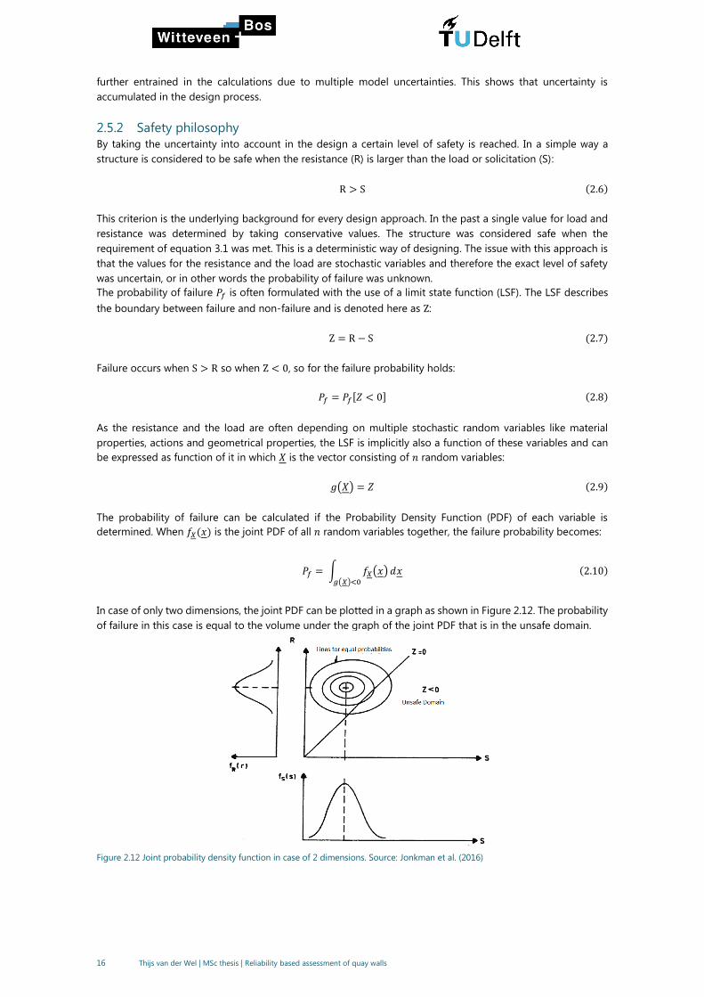
In case of only two dimensions, the joint PDF can be plotted in a graph as shown in Figure 2.12. The probability
of failure in this case is equal to the volume under the graph of the joint PDF that is in the unsafe domain.
Figure 2.12 Joint probability density function in case of 2 dimensions. Source: Jonkman et al. (2016)
17 Thijs van der Wel | MSc thesis | Reliability based assessment of quay walls
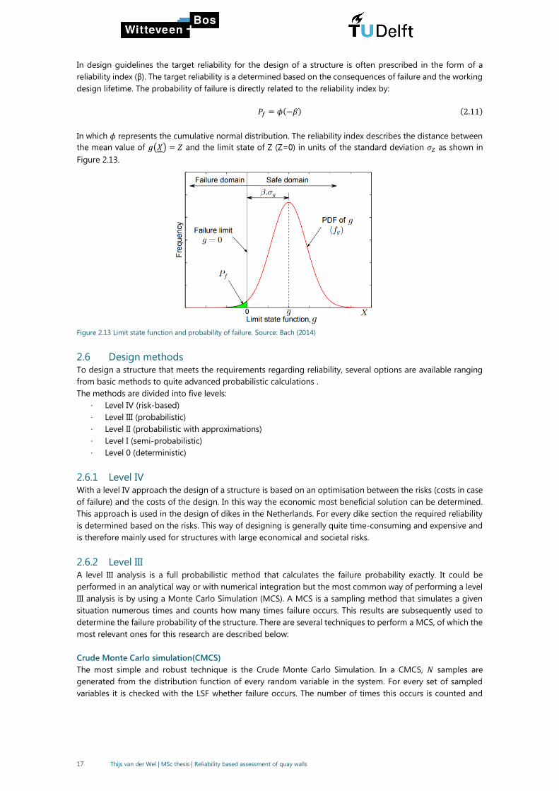
In design guidelines the target reliability for the design of a structure is often prescribed in the form of a
reliability index (β). The target reliability is a determined based on the consequences of failure and the working
design lifetime. The probability of failure is directly related to the reliability index by:
𝑃𝑓 = 𝜙(−𝛽) (2.11)
In which 𝜙 represents the cumulative normal distribution. The reliability index describes the distance between
the mean value of 𝑔(𝑋) = 𝑍 and the limit state of Z (Z=0) in units of the standard deviation 𝜎𝑍 as shown in
Figure 2.13.
Figure 2.13 Limit state function and probability of failure. Source: Bach (2014)
2.6 Design methods
To design a structure that meets the requirements regarding reliability, several options are available ranging
from basic methods to quite advanced probabilistic calculations .
The methods are divided into five levels:
· Level IV (risk-based)
· Level III (probabilistic)
· Level II (probabilistic with approximations)
· Level I (semi-probabilistic)
· Level 0 (deterministic)
2.6.1 Level IV
With a level IV approach the design of a structure is based on an optimisation between the risks (costs in case
of failure) and the costs of the design. In this way the economic most beneficial solution can be determined.
This approach is used in the design of dikes in the Netherlands. For every dike section the required reliability
is determined based on the risks. This way of designing is generally quite time-consuming and expensive and
is therefore mainly used for structures with large economical and societal risks.
2.6.2 Level III
A level III analysis is a full probabilistic method that calculates the failure probability exactly. It could be
performed in an analytical way or with numerical integration but the most common way of performing a level
III analysis is by using a Monte Carlo Simulation (MCS). A MCS is a sampling method that simulates a given
situation numerous times and counts how many times failure occurs. This results are subsequently used to
determine the failure probability of the structure. There are several techniques to perform a MCS, of which the
most relevant ones for this research are described below:
Crude Monte Carlo simulation(CMCS)
The most simple and robust technique is the Crude Monte Carlo Simulation. In a CMCS, 𝑁 samples are
generated from the distribution function of every random variable in the system. For every set of sampled
variables it is checked with the LSF whether failure occurs. The number of times this occurs is counted and

18 Thijs van der Wel | MSc thesis | Reliability based assessment of quay walls
when all realisation are performed, the probability of failure is calculated by dividing the number of failures
𝑁𝑓by the total number of samples 𝑁:
𝑃𝑓 =𝑁𝑓
𝑁(2.12)
The number of required simulations depends on the probability of failure and the desired accuracy of the
answer. In case 𝑃𝑓 ≪ 0, the chance of sampling failure is very low and therefore the amount of required
simulations increase rapidly. The minimal number of samples can be determined based on the probability of
failure and the target accuracy, defined by the coefficient of variation 𝑉(𝑃𝑓) (Waarts, 2000):
𝑁 >1
𝑉(𝑃𝑓)2 (
1
𝑃𝑓− 1) (2.13)
For structural systems the reliability index is often desired to be around 𝛽=4 (→ 𝑃𝑓 = 3.2 ∗ 10−5). When a target
𝑉(𝛽) of 0.05 is assumed acceptable, the minimum number of samples can be approximated by translating
𝑉(𝛽) = 0.05 to 𝑉(𝑃𝑓) = 0.57 and filling this into the equation above:
𝑁 >1
0.572(1
𝑃𝑓− 1) ≈
3
𝑃𝑓→ 𝑁 >
3
3.2 ∗ 10−5> 100,000
The minimal required number of calculations in this case is around 100,000. When performing this amount of
computations in a reliability analysis on a FEM-Model, the computational time is in the order of weeks,
depending on the size of the Finite Element Model and the computational power. Therefore several other
types of sampling methods have been developed that require less computations. Schweckendiek (2006)
evaluated the most common types of sampling methods on the applicability in structural reliability
computations. Aside from the calculation effort also other aspects were considered:
· the accuracy of the method
· the applicability in a system analysis
· the need for prior knowledge (which is often not available)
The most suitable sampling methods, available for use, are Directional Sampling and Directional Adaptive
Response Sampling.
Directional Sampling (DS)
Directional Sampling is quite different from a standard CMCS, but it is still based on sampling of random
variables. The method is an iterative process in which multiple vectors are sampled and scaled up to a length
for which holds 𝑍 = 0. The method is carried out in the u-space. This means that the random variables are
transformed to independent standard normal variables. The method can be explained by the steps described
by Schweckendiek (2006):
1 The origin of the u-vector is determined with a mean (or median) value calculation in 𝑢 = 0.
2 A point in the parameter space is generated from the random joint probability function. The vector 𝑢
is defined as the vector with its starting in the origin and the randomly generated point as end point.
3 The vector is scaled to a predefined length |𝑢| = 𝑢0 (often 𝑢0 is chosen as 1=unit vector). In this way
only the direction of the vector is kept as information of the random realization. Thereafter a Limit
State Function Evaluation (LSFE) is carried out in this point.

19 Thijs van der Wel | MSc thesis | Reliability based assessment of quay walls
Figure 2.14 Directional Sampling carried out in a 2-dimensional u-space (steps 1 to 3). Source: Schweckendiek (2006)
4 The vector is scaled with a factor λ ( λ ≥ 0) in an iterative procedure until the LSF is equal to zero (𝑍 =
0). This requires a LSFE for every time the vector is scaled, which is of importance for the computational
time.
Figure 2.15 Scaling of the vector with λ until the limit state function is found. Source: Schweckendiek (2006)
5 ∑ λ𝑖2𝑛
𝑖=1 is 𝜒2-distributed with n degrees of freedom. If λ was constant for all directions, the probability
of failure could be written as:
𝑃𝑓 = 1 − 𝜒2(λ2, 𝑛) (2.14)
If we have N random realisations of 𝑢 with different results for λ, the failure probability is estimated as:
𝑃𝑓 =1
𝑁∑ (1 − 𝜒2(λ𝑖
2, 𝑛)𝑁
𝑗=1)(2.15)
The corresponding variance for N realisations is:
𝜎𝑃𝑓2 =
1
𝑁(𝑁−1)∑ (𝑃𝑗 − 𝑃𝑓)
2𝑁𝑗=1 with 𝑃𝑗 = 1 − 𝜒2(λ𝑗
2, 𝑛)
6 The steps 1 till 5 are repeated until the accuracy in terms of variance is below a desired value. Other
stop criteria are also possible, for instance a maximum number of calculations.
2.6.3 Level II
With a level II analyses the failure probability is still explicitly calculated, but the problem is simplified by using
approximations of the random variables and the limit state function. It effects in considerable less
computational effort while the degree of accuracy is almost the same as for level III methods in many cases.
For complicated (highly non-linear) limit state functions and non-normally distributed random variables the
method becomes less accurate. Another important aspect is that a level II analysis cannot be used for a
complete system with multiple failure modes. For every failure mode the failure probability has to be calculated
20 Thijs van der Wel | MSc thesis | Reliability based assessment of quay walls
separately and therefore system effects are not taken into account when determining the system reliability.
Despite these limitations it is a very useful method.
First Order Reliability Method (FORM)
The most commonly applied level II analysis is the First Order Reliability Method introduced by Hasofer and
Lind (1974). The term First Order refers to the linearization of the limit state function, which is a first order
Taylor approximation. The theory can be explained using two uncorrelated normally distributed variables.
These variables are transformed into normalized variables (variables with 𝜇 = 0 and𝜎 = 1) by:
𝑈𝑖 =𝑋𝑖 − 𝜇𝑖𝜎𝑖
(2.16)
With resistance and load described by respectively 𝜇𝑅 and 𝜎𝑅 and 𝜇𝑆 and 𝜎𝑆, the limit state function 𝑔(𝑋) =
𝑅 − 𝑆 = 0 can be rewritten as function of the normalized variables:
𝑔(𝑈) = 𝜎𝑅𝑈𝑅 − 𝜎𝑆𝑈𝑆 + (𝜇𝑅 − 𝜇𝑆) = 0 (2.17)
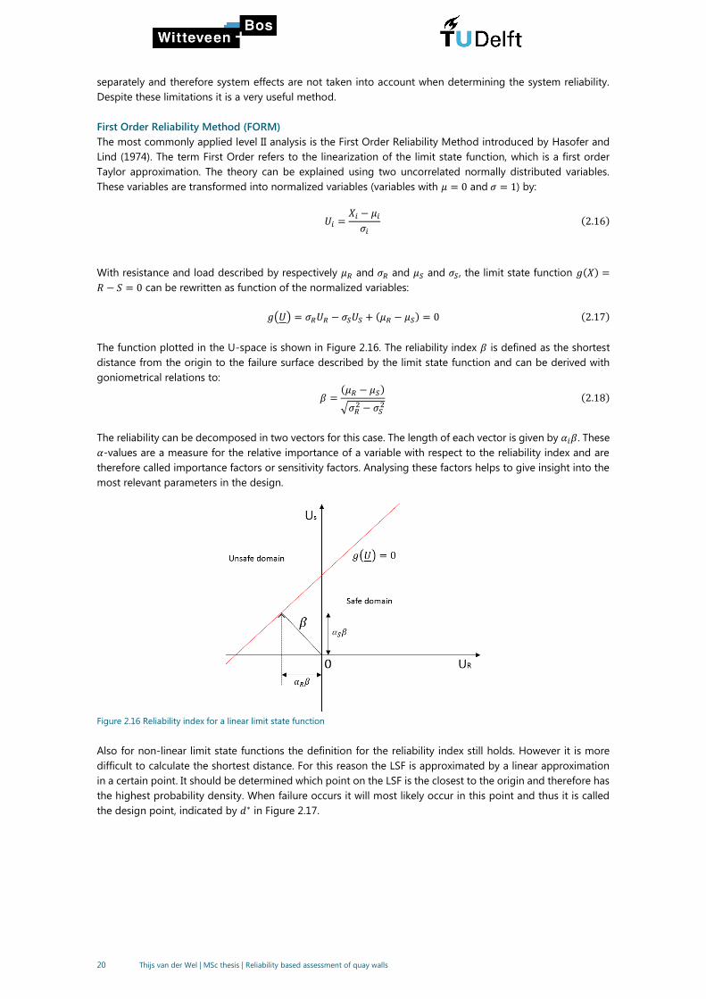
The function plotted in the U-space is shown in Figure 2.16. The reliability index 𝛽 is defined as the shortest
distance from the origin to the failure surface described by the limit state function and can be derived with
goniometrical relations to:
𝛽 =(𝜇𝑅 − 𝜇𝑆)
√𝜎𝑅2 − 𝜎𝑆
2(2.18)
The reliability can be decomposed in two vectors for this case. The length of each vector is given by 𝛼𝑖𝛽. These
𝛼-values are a measure for the relative importance of a variable with respect to the reliability index and are
therefore called importance factors or sensitivity factors. Analysing these factors helps to give insight into the
most relevant parameters in the design.
Figure 2.16 Reliability index for a linear limit state function
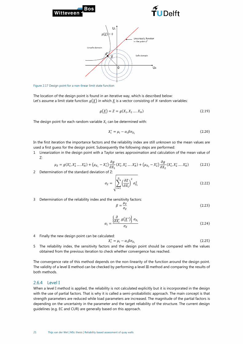
Also for non-linear limit state functions the definition for the reliability index still holds. However it is more
difficult to calculate the shortest distance. For this reason the LSF is approximated by a linear approximation
in a certain point. It should be determined which point on the LSF is the closest to the origin and therefore has
the highest probability density. When failure occurs it will most likely occur in this point and thus it is called
the design point, indicated by 𝑑∗ in Figure 2.17.
21 Thijs van der Wel | MSc thesis | Reliability based assessment of quay walls
Figure 2.17 Design point for a non-linear limit state function
The location of the design point is found in an iterative way, which is described below:
Let’s assume a limit state function 𝑔(𝑋) in which 𝑋 is a vector consisting of 𝑁 random variables:
𝑔(𝑋) = 𝑍 = 𝑔(𝑋1, 𝑋2… .𝑋𝑁) (2.19)
The design point for each random variable 𝑋𝑖 can be determined with:
𝑋𝑖∗ = 𝜇𝑖 − 𝛼𝑖𝛽𝜎𝑋𝑖 (2.20)
In the first iteration the importance factors and the reliability index are still unknown so the mean values are
used a first guess for the design point. Subsequently the following steps are performed:
1 Linearization in the design point with a Taylor series approximation and calculation of the mean value of
Z:
𝜇𝑍 = 𝑔(𝑋1∗, 𝑋2
∗… .𝑋𝑁∗ ) + (𝜇𝑋1 − 𝑋1
∗)𝜕𝑔
𝜕𝑋1(𝑋1
∗, 𝑋2∗… .𝑋𝑁
∗ ) + (𝜇𝑋2 − 𝑋2∗)
𝜕𝑔
𝜕𝑋2(𝑋1
∗, 𝑋2∗… .𝑋𝑁
∗ ) (2.21)
2 Determination of the standard deviation of Z:
𝜎𝑍 = √∑(𝜕𝑍
𝜕𝑋𝑖)2
𝜎𝑋𝑖2
𝑛
𝑖=1
(2.22)
3 Determination of the reliability index and the sensitivity factors:
𝛽 =𝜇𝑍𝜎𝑍
(2.23)
𝛼𝑖 ={𝜕𝜕𝑋𝑖
𝑔(𝑋∗)} 𝜎𝑋𝑖
𝜎𝑍(2.24)
4 Finally the new design point can be calculated:
𝑋𝑖∗ = 𝜇𝑖 − 𝛼𝑖𝛽𝜎𝑋𝑖 (2.25)
5 The reliability index, the sensitivity factors and the design point should be compared with the values
obtained from the previous iteration to check whether convergence has reached.
The convergence rate of this method depends on the non-linearity of the function around the design point.
The validity of a level II method can be checked by performing a level III method and comparing the results of
both methods.
2.6.4 Level I
When a level I method is applied, the reliability is not calculated explicitly but it is incorporated in the design
with the use of partial factors. That is why it is called a semi-probabilistic approach. The main concept is that
strength parameters are reduced while load parameters are increased. The magnitude of the partial factors is
depending on the uncertainty in the parameter and the target reliability of the structure. The current design
guidelines (e.g. EC and CUR) are generally based on this approach.

22 Thijs van der Wel | MSc thesis | Reliability based assessment of quay walls
The magnitude of parameters can be divided into three types:
· Mean values
· Characteristic values
· Design values
The definition of mean values speaks for itself. Characteristic values are values with a prescribed probability of
not being exceeded. Generally, values with a low exceedance probability (5%) are used in case of load
parameters and values with a high exceedance probability (95%) in case of strength parameters. Depending
on the parameter type also the mean value is sometimes used as characteristic value. The design values are
calculated by dividing or multiplying the characteristic values by partial factors. For the calculation of a design
resistance parameter holds:
𝑋𝑅,𝑑 =𝑋𝑅,𝑘𝛾𝑅,𝑑
(2.26)
Where
𝑋𝑅,𝑑 design value of a resistance parameter
𝑋𝑅,𝑘 characteristic value of a resistance parameter
𝛾𝑅,𝑑 partial safety factor for the corresponding resistance parameter
For a load parameter holds:
𝑋𝑆,𝑑 = 𝑋𝑆,𝑘 ∗ 𝛾𝑆,𝑑 (2.27)
The design load and the design strength of a structure can be expressed as function of the design parameters:
𝑅𝑑 = 𝑅(𝑋𝑅,𝑑1, 𝑋𝑅,𝑑2, … . . 𝑋𝑅,𝑑𝑛)
𝑆𝑑 = 𝑆(𝑋𝑆,𝑑1, 𝑋𝑆,𝑑2, … . . 𝑋𝑆,𝑑𝑛)
The design is assumed to be safe when for the limit state holds:
𝑅𝑑 ≥ 𝑆𝑑
For the simple case of a single load and resistance parameter, this principle is shown in Figure 2.18.
Figure 2.18 Principle of design load and design resistance. Source: Jonkman et al. (2016)
The partial safety factors are either determined in an empirical way or a probabilistic way (Figure 2.19). The
empirical method is based on the calibration of a long experience in building history and has no or few
probabilistic background.

23 Thijs van der Wel | MSc thesis | Reliability based assessment of quay walls
Figure 2.19 Methods to arrive at partial factors. Source: NEN-EN 1990 (2002)
A more mathematical approach is the calibration of the partial factors with a probabilistic calculation using a
level II method. In this way the reliability index obtained from the level II analysis is incorporated in the partial
factors of the level I method. With a FORM calculation the design point of every random parameter is
determined, together with the sensitivity factors and the reliability index. This output can be used to determine
the partial factor. For a partial factor on a resistance parameter holds:
𝛾𝑅,𝑑 =𝑋𝑅,𝑘𝑋𝑅,𝑑
=𝜇𝑅 − 𝑘𝑅𝜎𝑅
𝜇𝑅 + 𝛼𝑅𝛽𝜎𝑅=
𝜇𝑅(1 − 𝑘𝑉𝑅)
𝜇𝑅(1 + 𝛼𝑅𝛽𝑉𝑅)=
1 − 𝑘𝑅𝑉𝑅1 + 𝛼𝑅𝛽𝑉𝑅
(2.28)
Where
𝑘 characteristic factor (for a normally distributed parameter and an exceedance probability of 5 or 95%,
a value of 1.645 is used)
𝑉𝑅 coefficient of variation: 𝑉𝑅 =𝜎𝑅
𝜇𝑅
𝛼𝑅 importance parameter obtained from the FORM analysis (in case of a favourable influence on the
reliability index, the 𝛼-value is returned as a negative value in FORM)
𝛽 target reliability index
𝜇𝑅 mean value of the concerned parameter
𝜎𝑅 standard deviation of the concerned parameter
In the same way the partial factor on a load parameter can be determined:
𝛾𝑆,𝑑 =𝑋𝑆,𝑑𝑋𝑆,𝑘
=𝜇𝑆 + 𝛼𝑆𝛽𝜎𝑆𝜇𝑆 + 𝑘𝜎𝑆
=1 + 𝛼𝑆𝛽𝑉𝑆1 + 𝑘𝑉𝑆
(2.29)
The partial factors in design guidelines are often calibrated on a few specific structures. This makes the
applicability of these factors doubtful in case of structures that deviate considerably from the calibrated
structures. This is partly taken into account by prescribing slightly conservative partial factors. The use of partial
factors can therefore result in a deviation of the actual reliability compared to the target reliability. With a full
probabilistic analysis this problem is avoided. Especially for one-of-a-kind structures the use of a full
probabilistic method can result in considerable cost savings due allowance for a more economical design.
2.6.5 Level 0
A very basic approach is the level 0 approach. With this method nominal values are taken for all the variables
after which one single global safety factor is applied. The structure is considered safe when the following
equation holds:
𝑅𝑛𝑜𝑚 ≥ 𝛾𝑆𝑛𝑜𝑚 (2.30)
24 Thijs van der Wel | MSc thesis | Reliability based assessment of quay walls
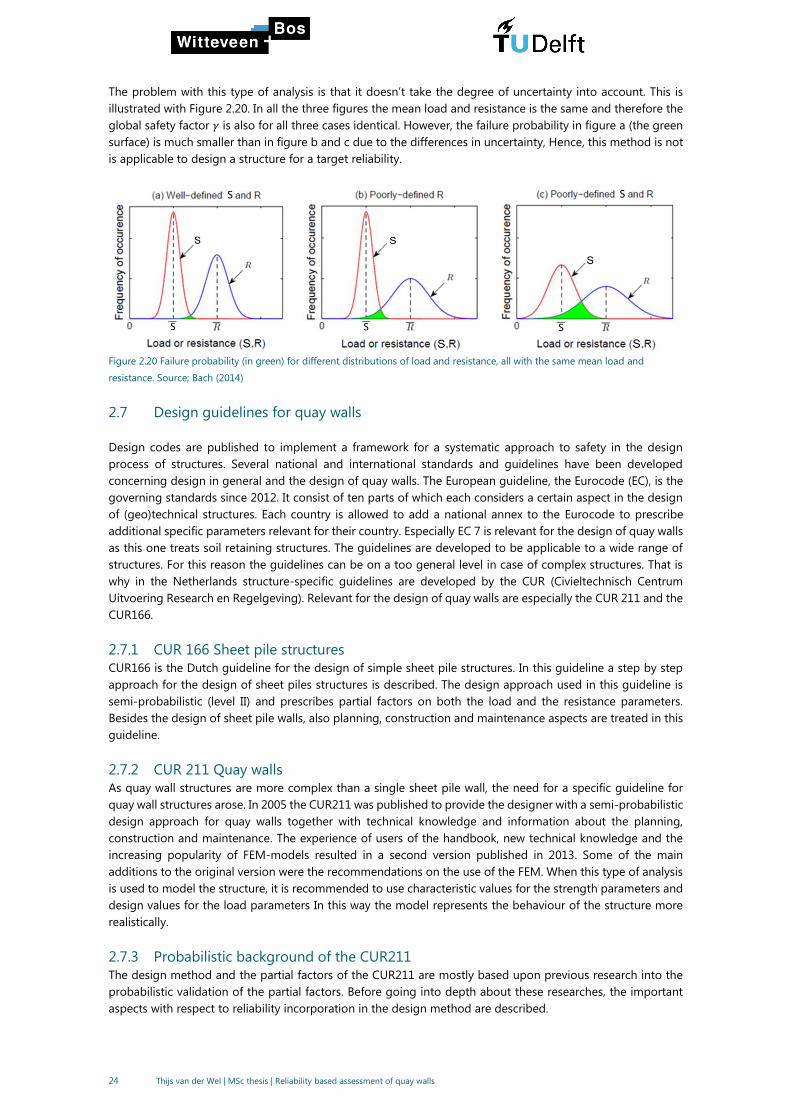
The problem with this type of analysis is that it doesn’t take the degree of uncertainty into account. This is
illustrated with Figure 2.20. In all the three figures the mean load and resistance is the same and therefore the
global safety factor 𝛾 is also for all three cases identical. However, the failure probability in figure a (the green
surface) is much smaller than in figure b and c due to the differences in uncertainty, Hence, this method is not
is applicable to design a structure for a target reliability.
Figure 2.20 Failure probability (in green) for different distributions of load and resistance, all with the same mean load and
resistance. Source; Bach (2014)
2.7 Design guidelines for quay walls
Design codes are published to implement a framework for a systematic approach to safety in the design
process of structures. Several national and international standards and guidelines have been developed
concerning design in general and the design of quay walls. The European guideline, the Eurocode (EC), is the
governing standards since 2012. It consist of ten parts of which each considers a certain aspect in the design
of (geo)technical structures. Each country is allowed to add a national annex to the Eurocode to prescribe
additional specific parameters relevant for their country. Especially EC 7 is relevant for the design of quay walls
as this one treats soil retaining structures. The guidelines are developed to be applicable to a wide range of
structures. For this reason the guidelines can be on a too general level in case of complex structures. That is
why in the Netherlands structure-specific guidelines are developed by the CUR (Civieltechnisch Centrum
Uitvoering Research en Regelgeving). Relevant for the design of quay walls are especially the CUR 211 and the
CUR166.
2.7.1 CUR 166 Sheet pile structures
CUR166 is the Dutch guideline for the design of simple sheet pile structures. In this guideline a step by step
approach for the design of sheet piles structures is described. The design approach used in this guideline is
semi-probabilistic (level II) and prescribes partial factors on both the load and the resistance parameters.
Besides the design of sheet pile walls, also planning, construction and maintenance aspects are treated in this
guideline.
2.7.2 CUR 211 Quay walls
As quay wall structures are more complex than a single sheet pile wall, the need for a specific guideline for
quay wall structures arose. In 2005 the CUR211 was published to provide the designer with a semi-probabilistic
design approach for quay walls together with technical knowledge and information about the planning,
construction and maintenance. The experience of users of the handbook, new technical knowledge and the
increasing popularity of FEM-models resulted in a second version published in 2013. Some of the main
additions to the original version were the recommendations on the use of the FEM. When this type of analysis
is used to model the structure, it is recommended to use characteristic values for the strength parameters and
design values for the load parameters In this way the model represents the behaviour of the structure more
realistically.
2.7.3 Probabilistic background of the CUR211
The design method and the partial factors of the CUR211 are mostly based upon previous research into the
probabilistic validation of the partial factors. Before going into depth about these researches, the important
aspects with respect to reliability incorporation in the design method are described.

25 Thijs van der Wel | MSc thesis | Reliability based assessment of quay walls
Important aspect of the approach of the CUR211
Before starting with the actual design of a quay wall, the starting points (e.g. bottom level, quay level and the
consequence class) should be agreed upon with the client. The consequence class (CC), or in the Netherlands
described as reliability class (RC), is selected from Table 2.3. For most quay walls in the Port of Rotterdam CC2
is applicable which corresponds to a reliability index of 3.8 and a failure probability of 7.2*10-5.
Table 2.3 Reliability/Consequence Classes for quay walls. Source: NEN-EN 1990 (2002)
The choice of the consequence class is determining the magnitude of the prescribed partial factors. The EC
describes three design approaches for the use of partial factors, whereas in the National Annex design
approach 3 is prescribed in the Netherlands. This implies partial factors on the material characteristics and
partial factors on the loads. The partial factors of the EC7 are based on calculations on simple quay walls.
Therefore probabilistic calculations are carried out for quay walls with a relieving platform to attain more
accurate partial factors. This has resulted in a set of partial factors for the load and resistant parameters. The
factors for the soil parameters are given as example in Table 2.4. For the partial factors of all the other variables
reference is made to the CUR 211.
Table 2.4 Partial safety factors on the soil parameters for quay walls with relieving platform. Source: NEN 9997 (2017)
Chapter 6 describes a step-wise approach to determine the safety with respect to all kinds of failure modes.
Only the ULS-check on the embedded depth, the bending moments, normal forces and shear forces in the
retaining structure and the anchor are highlighted here because of the slightly different approach that is used
compared to the NEN 9997. In the FEM-model representative values for the soil strength parameters should
be used instead of design values to better represent the actual failure behaviour. Thereafter the strength
parameters (𝜑 and c) are reduced by a prescribed factor with the ‘φ-c reduction’ method. Subsequently the
design values for the sectional forces are obtained.

26 Thijs van der Wel | MSc thesis | Reliability based assessment of quay walls
Previous research on the partial factors for quay walls
The design approach and the partial factors of the CUR 211 are based on several probabilistic calculations,
which go back to the development of the first CUR 166 in 1993. For this guideline (Calle & Spierenburg, 1991)
performed one of the first probabilistic analyses for an anchored sheet pile wall. It concerns a level II analysis
performed on the a spring model in the software program DAMWAND. In the research a fault tree was created
and the total failure space was divided into pieces. Mechanisms which are easy and cheap to improve were
given an low acceptable failure probability of ‘0.2p’ whereas the main failure mechanisms (passive resistance
failure, failure of the sheet pile profile, total instability, groundwater flow and anchor failure) were given a
failure space of ‘p’. The system was considered as a serial system with strong dependency between the different
failure mechanisms. The failure probability of a top event was calculated by fully counting the largest failure
probability and multiplying the other failure probabilities that are at the same level of the tree by ½ before
adding to the largest failure probability The obtained importance factors and reliability index of the level II
analysis were used to calculate the partial safety factors for the first CUR166. These values were later validated
by Havinga (2004) who concluded that the partial factors are resulting in more or less the correct reliability.
However, a quay wall differs quite much from a sheet pile wall and therefore Gemeentewerken Rotterdam
(Huijzer, 1996) conducted a research into the adaption of the partial factors of CUR166 to be applicable for
quay walls. This led to an adaption of the fault tree due to the addition of extra components (e.g. the concrete
superstructure and bearing piles). Also the division of the failure space has been changed as it appeared that
yielding of the sheet pile profile was the main failure mode. Subsequently a new set of partial factors was
determined.
de Grave (2002) was the first one to validate this new set of partial factors on four different existing quay walls
of which two of them were quay walls of EMO. He performed a level II analysis with the software package PC-
Dam (elasto-plastic spring model) and compared the results with the original design that was calculated in a
deterministic way. His main conclusions were:
· The partial factors on the soil parameters can remain the same
· The partial factor on the bending moment also result in the right reliability
· The outside water levels and ground water levels should not be considered as independent as it is a
too conservative assumption
It should be mentioned that the calculations were performed on a highly simplified model based on
conservative assumptions.
Wolters (2012) validated the partial factors based on a coupling of a PLAXIS-FORM and was therefore able to
model the structure and the soil-structure interaction much more accurate. One of the two case studies he
performed was on the EMO quay wall that is considered in this thesis. However, he adjusted the final design
of the structure in accordance with CUR166 to enable a comparison between the design code and the
calculation results. The combi-wall is placed vertical instead of under an angle. Due to this adjustment it was
necessary to add a second anchor row because otherwise the horizontal deformations at the top were larger
than the maximum of 50mm (requirement for the crane track).
Wolters stated that the soil mechanical failure is the most critical failure mechanism. With respect to economic
optimisation it should therefore not get a higher target reliability than bending wall failure or anchor failure.
As this results in a higher partial factor on the angle of internal friction. The failure space should be taken from
‘anchor failure in tension’ as this mechanism turned out to have a higher reliability than expected. Furthermore
he found out that there is a strong correlation between soil mechanical failure and bending wall failure,
whereas anchor failure shows little correlation with respect to those two mechanisms. Also the spatial
variability of the soil turned out to have a large influence on the magnitude of the partial factors
Other recommendations were:
· Use different safety factors per failure mechanism to prevent overdimensioning of elements
· Use higher partial safety factors on the internal angle of friction and soil stiffness parameters
· Use lower partial safety factors on the geometrical parameters
· Use mean values for cohesion, sheet-pile parameters and anchor diameter.
With respect to full probabilistic design of quay walls he recommended to perform probabilistic calculations
for every new quay wall to accomplish a more optimal design. However the use of FORM is doubtful. The
plastic behaviour of soil is non-linear and therefore the linear approximation with FORM is not always accurate.

27 Thijs van der Wel | MSc thesis | Reliability based assessment of quay walls
2.8 Conclusion
The topics described in this chapter has given a general overview of the most relevant existing knowledge
regarding the design of quay structures, the main types of uncertainties and available probabilistic methods.
This theory helped with composing the research methodology that is extensively described in the next
chapter.

28 Thijs van der Wel | MSc thesis | Reliability based assessment of quay walls
3
METHOD DESCRIPTION
As described in the first chapter, the objective of this thesis is to validate the current design approach and to
explore possibilities for case-specific load increase by performing probabilistic calculations.
The literature overview in the previous chapter showed that failure of the quay wall can be triggered by
numerous mechanisms and that there are multiple options regarding the modelling of the problem and the
type of probabilistic methods. Relevant questions that are answered in this chapter are:
· Which failure mechanisms are most relevant regarding the design of quay wall structures ?
· What is an appropriate limit state function for these failure mechanisms?
· Which probabilistic method is most suitable for assessing these LSFs and which software should be
used for this?
The answers to these questions have resulted in the research methodology that is applied on two case studies.
Both case studies are quay walls located in the Port of Rotterdam. The first case study considers a simple
double anchored combi-wall, whereas the second case study considers a quay wall with relieving platform. An
general overview of the applied approach is given shown in Figure 3.1.
Figure 3.1 Flowchart of research methodology

29 Thijs van der Wel | MSc thesis | Reliability based assessment of quay walls
3.1 Selection of Failure Mechanisms
In this subchapter a selection is made of the failure modes which will be assessed for the two case studies.
In chapter 2.4 an introduction on the fault tree of a quay wall is already given.
This fault tree of the CUR211 consists of 23 base events. It is for several reasons not possible and not desired
to calculate all their failure probabilities. This thesis is limited to the determination of the failure probability of:
· Events with a significant influence on the overall failure probability of a quay wall
· Events that can be assessed by using a coupling between Plaxis and an appropriate probabilistic
method
To determine the contribution of each failure mode to the overall failure probability, the fault tree of CUR211
(2005) (Appendix A) was checked. In this fault tree most of the failure modes are assigned with a target
reliability index. The importance of a failure mode can therefore be interpreted from its assigned target
reliability. The division of the failure space within this tree is for a large part based on economical choices.
Failure modes that are expensive to prevent are assigned with a low target reliability and failure modes that
can be prevented with small investments were given a high target reliability. In this way, the most economically
beneficial solution is created. When looking at the distribution of the construction costs for combi-walls with
a concrete relieving platform as shown in Figure 3.2, it is obvious that the steel of the combi-wall has the
largest contribution to the total cost. Thereafter follows the concrete superstructure, which falls mainly under
the category concrete, reinforcing steel and labour.
Figure 3.2 Distribution of costs as a percentage of the construction cost for combi-wall structures with a
concrete superstructure. Source: CUR211 (2013)
It is therefore not surprising that failure of the sheet pile wall is provided with the most failure space. Thereafter
follows the failure of the superstructure and subsequently the bearing piles and the tension members. Soil
mechanical failure is included within multiple subcomponents of the previously mentioned failure modes. It
covers amongst others the following events:
· Passive resistance in front of the retaining wall inadequate
· Lack of equilibrium (Bishop slip circle)
· Heave
· Piping
· Krantz stability inadequate
· Shear resistance of anchorage inadequate
Not all of the soil mechanical failure modes can be assessed using Plaxis coupled with reliability methods.
Piping is an example of this. Besides, it is hardly possible to assess the reliability of soil mechanical failure
modes individually as the most dominant failure mode is triggered first.
Previous experience with coupling FORM to Plaxis (see chapter 3.3) has shown that the reliability of steel
structural elements can be assessed relatively well, if soil mechanical failure is non-dominant. The
determination of the reliability regarding soil mechanical failure caused significantly more problems with
convergence in previous research. However new developments in the robustness of FORM calculations enables
for this failure mechanism to be assessed more easily.

30 Thijs van der Wel | MSc thesis | Reliability based assessment of quay walls
Conclusion
Yielding of the combi-wall profile and soil mechanical failure are dominant failure modes of which the
reliability can be assessed with FORM and are therefore included. Yielding of the anchor profile is often non-
dominant but can be assessed with relatively little effort and is therefore included as well. The selected
failure mechanisms are marked in the fault tree in Figure 3.3. Each failure mechanism will be treated
separately, in which simultaneous failure of other mechanisms is neglected (except when it concerns soil
mechanical failure).
Figure 3.3 Selected failure mechanisms. Adapted from: CUR211 (2013)
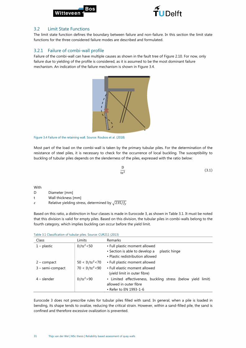
31 Thijs van der Wel | MSc thesis | Reliability based assessment of quay walls
3.2 Limit State Functions
The limit state function defines the boundary between failure and non-failure. In this section the limit state
functions for the three considered failure modes are described and formulated.
3.2.1 Failure of combi-wall profile
Failure of the combi-wall can have multiple causes as shown in the fault tree of Figure 2.10. For now, only
failure due to yielding of the profile is considered, as it is assumed to be the most dominant failure
mechanism. An indication of the failure mechanism is shown in Figure 3.4.
Figure 3.4 Failure of the retaining wall. Source: Roubos et al. (2018)
Most part of the load on the combi-wall is taken by the primary tubular piles. For the determination of the
resistance of steel piles, it is necessary to check for the occurrence of local buckling. The susceptibility to
buckling of tubular piles depends on the slenderness of the piles, expressed with the ratio below:
D
tε2(3.1)
With
D Diameter [mm]
t Wall thickness [mm]
휀 Relative yielding stress, determined by √235/𝑓𝑦
Based on this ratio, a distinction in four classes is made in Eurocode 3, as shown in Table 3.1. It must be noted
that this division is valid for empty piles. Based on this division, the tubular piles in combi-walls belong to the
fourth category, which implies buckling can occur before the yield limit.
Table 3.1 Classification of tubular piles. Source: CUR211 (2013)
Class Limits Remarks
1 – plastic
D/tε2<50 • Full plastic moment allowed
• Section is able to develop a plastic hinge
• Plastic redistribution allowed
2 – compact 50 < D/tε2<70 • Full plastic moment allowed
3 – semi-compact 70 < D/tε2<90 • Full elastic moment allowed
(yield limit in outer fibre)
4 – slender D/tε2>90 • Limited effectiveness, buckling stress (below yield limit)
allowed in outer fibre
• Refer to EN 1993-1-6
Eurocode 3 does not prescribe rules for tubular piles filled with sand. In general, when a pile is loaded in
bending, its shape tends to ovalize, reducing the critical strain. However, within a sand-filled pile, the sand is
confined and therefore excessive ovalization is prevented.
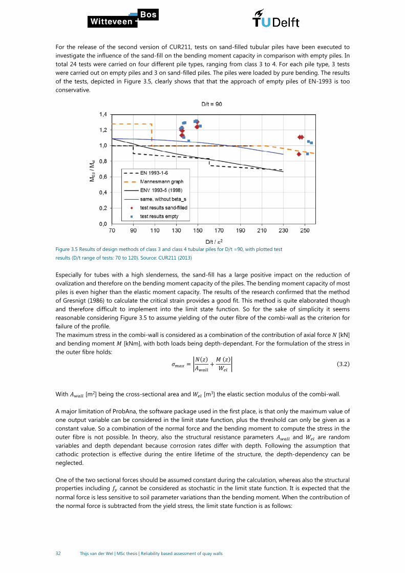
32 Thijs van der Wel | MSc thesis | Reliability based assessment of quay walls
For the release of the second version of CUR211, tests on sand-filled tubular piles have been executed to
investigate the influence of the sand-fill on the bending moment capacity in comparison with empty piles. In
total 24 tests were carried on four different pile types, ranging from class 3 to 4. For each pile type, 3 tests
were carried out on empty piles and 3 on sand-filled piles. The piles were loaded by pure bending. The results
of the tests, depicted in Figure 3.5, clearly shows that that the approach of empty piles of EN-1993 is too
conservative.
Figure 3.5 Results of design methods of class 3 and class 4 tubular piles for D/t =90, with plotted test
results (D/t range of tests: 70 to 120). Source: CUR211 (2013)
Especially for tubes with a high slenderness, the sand-fill has a large positive impact on the reduction of
ovalization and therefore on the bending moment capacity of the piles. The bending moment capacity of most
piles is even higher than the elastic moment capacity. The results of the research confirmed that the method
of Gresnigt (1986) to calculate the critical strain provides a good fit. This method is quite elaborated though
and therefore difficult to implement into the limit state function. So for the sake of simplicity it seems
reasonable considering Figure 3.5 to assume yielding of the outer fibre of the combi-wall as the criterion for
failure of the profile.
The maximum stress in the combi-wall is considered as a combination of the contribution of axial force 𝑁 [kN]
and bending moment 𝑀 [kNm], with both loads being depth-dependant. For the formulation of the stress in
the outer fibre holds:
𝜎𝑚𝑎𝑥 = |𝑁(𝑧)
𝐴𝑤𝑎𝑙𝑙+𝑀(𝑧)
𝑊𝑒𝑙| (3.2)
With 𝐴𝑤𝑎𝑙𝑙 [m2] being the cross-sectional area and 𝑊𝑒𝑙 [m
3] the elastic section modulus of the combi-wall.
A major limitation of ProbAna, the software package used in the first place, is that only the maximum value of
one output variable can be considered in the limit state function, plus the threshold can only be given as a
constant value. So a combination of the normal force and the bending moment to compute the stress in the
outer fibre is not possible. In theory, also the structural resistance parameters 𝐴𝑤𝑎𝑙𝑙 and 𝑊𝑒𝑙 are random
variables and depth dependant because corrosion rates differ with depth. Following the assumption that
cathodic protection is effective during the entire lifetime of the structure, the depth-dependency can be
neglected.
One of the two sectional forces should be assumed constant during the calculation, whereas also the structural
properties including 𝑓𝑦 cannot be considered as stochastic in the limit state function. It is expected that the
normal force is less sensitive to soil parameter variations than the bending moment. When the contribution of
the normal force is subtracted from the yield stress, the limit state function is as follows:
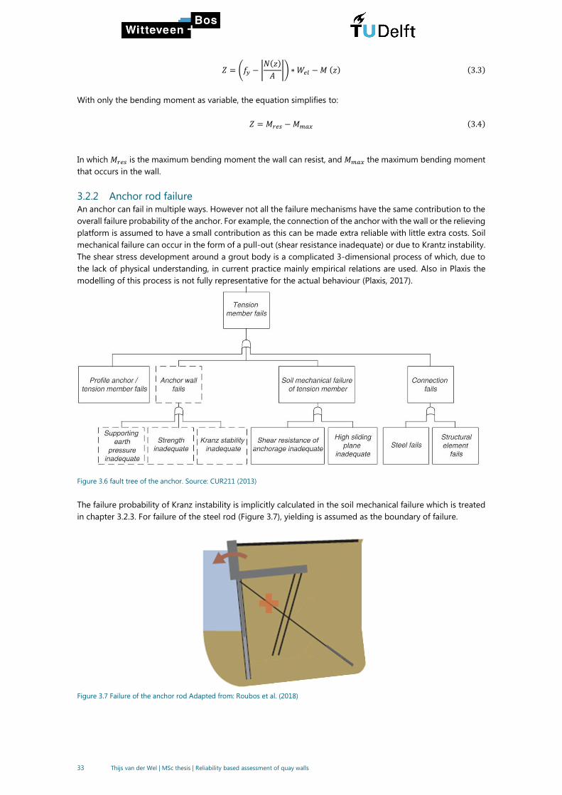
33 Thijs van der Wel | MSc thesis | Reliability based assessment of quay walls
𝑍 = (𝑓𝑦 − |𝑁(𝑧)
𝐴|) ∗ 𝑊𝑒𝑙 −𝑀(𝑧) (3.3)
With only the bending moment as variable, the equation simplifies to:
𝑍 = 𝑀𝑟𝑒𝑠 −𝑀𝑚𝑎𝑥 (3.4)
In which 𝑀𝑟𝑒𝑠 is the maximum bending moment the wall can resist, and 𝑀𝑚𝑎𝑥 the maximum bending moment
that occurs in the wall.
3.2.2 Anchor rod failure
An anchor can fail in multiple ways. However not all the failure mechanisms have the same contribution to the
overall failure probability of the anchor. For example, the connection of the anchor with the wall or the relieving
platform is assumed to have a small contribution as this can be made extra reliable with little extra costs. Soil
mechanical failure can occur in the form of a pull-out (shear resistance inadequate) or due to Krantz instability.
The shear stress development around a grout body is a complicated 3-dimensional process of which, due to
the lack of physical understanding, in current practice mainly empirical relations are used. Also in Plaxis the
modelling of this process is not fully representative for the actual behaviour (Plaxis, 2017).
Figure 3.6 fault tree of the anchor. Source: CUR211 (2013)
The failure probability of Kranz instability is implicitly calculated in the soil mechanical failure which is treated
in chapter 3.2.3. For failure of the steel rod (Figure 3.7), yielding is assumed as the boundary of failure.
Figure 3.7 Failure of the anchor rod Adapted from: Roubos et al. (2018)

34 Thijs van der Wel | MSc thesis | Reliability based assessment of quay walls
The most important load on the anchor is the axial tension force. Due to uneven settlements along the rod, it
is also possible that it is subjected to bending moments. Here it is assumed that the anchor rod will only be
subjected to axial forces and that skin friction along the rod can be neglected. This simplifies the limit state
function to:
𝑍 = 𝑓𝑦𝐴𝑎𝑛𝑐ℎ𝑜𝑟 − 𝑁𝑆 (3.5)
With the resistance consisting of the yield stress 𝑓𝑦 [kN/m2] and the cross-sectional area of the rod 𝐴𝑎𝑛𝑐ℎ𝑜𝑟
[m2]. Considering them as constants yields the following simplified equation:
𝑍 = 𝑁𝑅 − 𝑁𝑆 (3.6)
With 𝑁𝑅 [kN] representing the strength of the anchor and 𝑁𝑆 [kN] the occurring force in the anchor.
Again, the yield limit and the cross-sectional area cannot be considered as random variables in the LSF using
ProbAna. It should be verified whether assuming them as deterministic is a valid assumption.
3.2.3 Soil mechanical failure
As already mentioned in chapter 3.1, soil mechanical failure can be triggered in multiple ways. An impression
of the failure modes is shown in Figure 3.8.
Figure 3.8 Impression of geotechnical failure modes. Left: Failure of the passive wedge, Middle: Failure of anchor system, Right:
Macro instability. Source: Roubos et al. (2018)
The most common way to express the stability of a soil body in Plaxis is with the use of the built in ‘φ-c
reduction’ method. With this method, the strength parameters of the soil are reduced with small steps until
the soil has just enough strength to maintain equilibrium. The required reduction on the strength parameters
is presented as the Multiplier safety factor ( ∑𝑀𝑠𝑓), which can be considered as the Factor of Safety for the
soil:
𝑀𝑠𝑓 =𝑎𝑣𝑎𝑖𝑙𝑎𝑏𝑙𝑒𝑠𝑡𝑟𝑒𝑛𝑔𝑡ℎ
𝑚𝑖𝑛𝑖𝑚𝑎𝑙𝑟𝑒𝑞𝑢𝑖𝑟𝑒𝑑𝑠𝑡𝑟𝑒𝑛𝑔ℎ𝑡=
𝑐
𝑐𝑟=
tan(𝜑)
tan(𝜑𝑟)(3.7)
In which 𝑐𝑟 and 𝜑𝑟 are the reduced strength parameters. It must be noted that not 𝜑𝑟 is reduced but tan(𝜑𝑟)
to keep the reduction of the shear strength linear. The boundary between failure and non-failure is reached
when the safety factor reaches a value of 1.0. Thus in theory the limit state function for a probabilistic analysis
should be:
𝑍 = 𝑀𝑠𝑓 − 1.0 (3.8)
Experience in combining this limit state formulation with a FORM analysis is gathered by Wolters (2012) and
Manoj (2017). Wolters faced problems with soil body collapse in earlier phases than the considered phase
because the iterations are performed on the edge of failure. As soil body collapse is not allowed during FORM
analysis in his case, he raised the threshold to 1.1 and assumed the impact of this measure on the importance
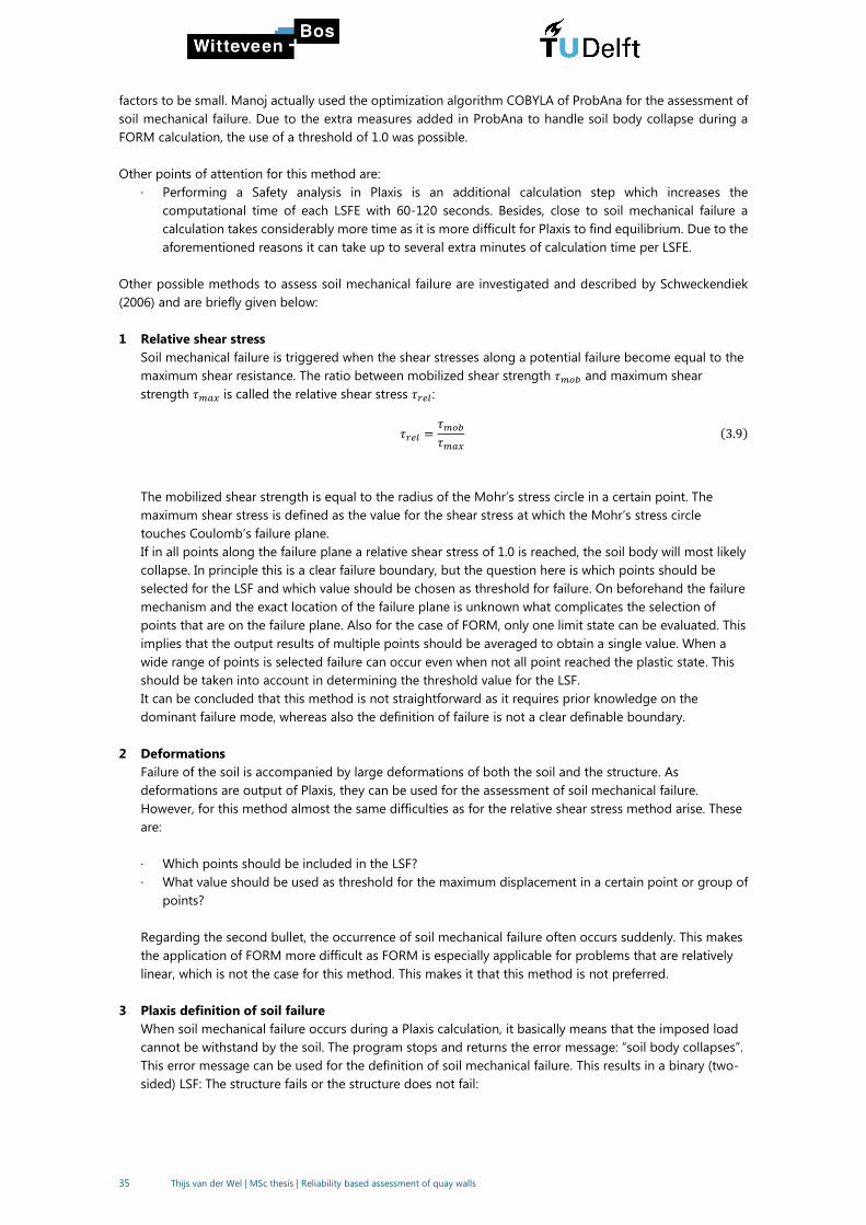
35 Thijs van der Wel | MSc thesis | Reliability based assessment of quay walls
factors to be small. Manoj actually used the optimization algorithm COBYLA of ProbAna for the assessment of
soil mechanical failure. Due to the extra measures added in ProbAna to handle soil body collapse during a
FORM calculation, the use of a threshold of 1.0 was possible.
Other points of attention for this method are:
· Performing a Safety analysis in Plaxis is an additional calculation step which increases the
computational time of each LSFE with 60-120 seconds. Besides, close to soil mechanical failure a
calculation takes considerably more time as it is more difficult for Plaxis to find equilibrium. Due to the
aforementioned reasons it can take up to several extra minutes of calculation time per LSFE.
Other possible methods to assess soil mechanical failure are investigated and described by Schweckendiek
(2006) and are briefly given below:
1 Relative shear stress
Soil mechanical failure is triggered when the shear stresses along a potential failure become equal to the
maximum shear resistance. The ratio between mobilized shear strength 𝜏𝑚𝑜𝑏 and maximum shear
strength 𝜏𝑚𝑎𝑥 is called the relative shear stress 𝜏𝑟𝑒𝑙 :
𝜏𝑟𝑒𝑙 =𝜏𝑚𝑜𝑏
𝜏𝑚𝑎𝑥
(3.9)
The mobilized shear strength is equal to the radius of the Mohr’s stress circle in a certain point. The
maximum shear stress is defined as the value for the shear stress at which the Mohr’s stress circle
touches Coulomb’s failure plane.
If in all points along the failure plane a relative shear stress of 1.0 is reached, the soil body will most likely
collapse. In principle this is a clear failure boundary, but the question here is which points should be
selected for the LSF and which value should be chosen as threshold for failure. On beforehand the failure
mechanism and the exact location of the failure plane is unknown what complicates the selection of
points that are on the failure plane. Also for the case of FORM, only one limit state can be evaluated. This
implies that the output results of multiple points should be averaged to obtain a single value. When a
wide range of points is selected failure can occur even when not all point reached the plastic state. This
should be taken into account in determining the threshold value for the LSF.
It can be concluded that this method is not straightforward as it requires prior knowledge on the
dominant failure mode, whereas also the definition of failure is not a clear definable boundary.
2 Deformations
Failure of the soil is accompanied by large deformations of both the soil and the structure. As
deformations are output of Plaxis, they can be used for the assessment of soil mechanical failure.
However, for this method almost the same difficulties as for the relative shear stress method arise. These
are:
· Which points should be included in the LSF?
· What value should be used as threshold for the maximum displacement in a certain point or group of
points?
Regarding the second bullet, the occurrence of soil mechanical failure often occurs suddenly. This makes
the application of FORM more difficult as FORM is especially applicable for problems that are relatively
linear, which is not the case for this method. This makes it that this method is not preferred.
3 Plaxis definition of soil failure
When soil mechanical failure occurs during a Plaxis calculation, it basically means that the imposed load
cannot be withstand by the soil. The program stops and returns the error message: “soil body collapses”.
This error message can be used for the definition of soil mechanical failure. This results in a binary (two-
sided) LSF: The structure fails or the structure does not fail:
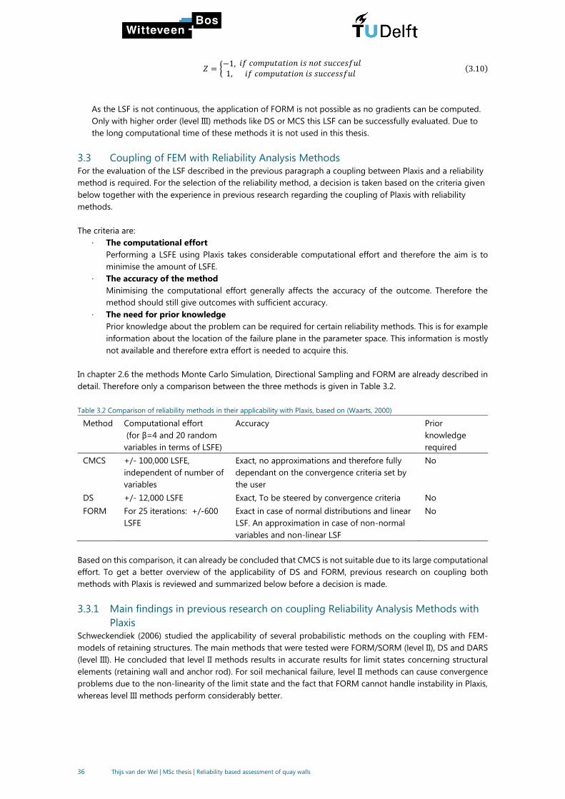
36 Thijs van der Wel | MSc thesis | Reliability based assessment of quay walls
𝑍 = {−1,1,𝑖𝑓𝑐𝑜𝑚𝑝𝑢𝑡𝑎𝑡𝑖𝑜𝑛𝑖𝑠𝑛𝑜𝑡𝑠𝑢𝑐𝑐𝑒𝑠𝑓𝑢𝑙𝑖𝑓𝑐𝑜𝑚𝑝𝑢𝑡𝑎𝑡𝑖𝑜𝑛𝑖𝑠𝑠𝑢𝑐𝑐𝑒𝑠𝑠𝑓𝑢𝑙
(3.10)
As the LSF is not continuous, the application of FORM is not possible as no gradients can be computed.
Only with higher order (level III) methods like DS or MCS this LSF can be successfully evaluated. Due to
the long computational time of these methods it is not used in this thesis.
3.3 Coupling of FEM with Reliability Analysis Methods
For the evaluation of the LSF described in the previous paragraph a coupling between Plaxis and a reliability
method is required. For the selection of the reliability method, a decision is taken based on the criteria given
below together with the experience in previous research regarding the coupling of Plaxis with reliability
methods.
The criteria are:
· The computational effort
Performing a LSFE using Plaxis takes considerable computational effort and therefore the aim is to
minimise the amount of LSFE.
· The accuracy of the method
Minimising the computational effort generally affects the accuracy of the outcome. Therefore the
method should still give outcomes with sufficient accuracy.
· The need for prior knowledge
Prior knowledge about the problem can be required for certain reliability methods. This is for example
information about the location of the failure plane in the parameter space. This information is mostly
not available and therefore extra effort is needed to acquire this.
In chapter 2.6 the methods Monte Carlo Simulation, Directional Sampling and FORM are already described in
detail. Therefore only a comparison between the three methods is given in Table 3.2.
Table 3.2 Comparison of reliability methods in their applicability with Plaxis, based on (Waarts, 2000)
Method Computational effort
(for β=4 and 20 random
variables in terms of LSFE)
Accuracy Prior
knowledge
required
CMCS +/- 100,000 LSFE,
independent of number of
variables
Exact, no approximations and therefore fully
dependant on the convergence criteria set by
the user
No
DS +/- 12,000 LSFE Exact, To be steered by convergence criteria No
FORM For 25 iterations: +/-600
LSFE
Exact in case of normal distributions and linear
LSF. An approximation in case of non-normal
variables and non-linear LSF
No
Based on this comparison, it can already be concluded that CMCS is not suitable due to its large computational
effort. To get a better overview of the applicability of DS and FORM, previous research on coupling both
methods with Plaxis is reviewed and summarized below before a decision is made.
3.3.1 Main findings in previous research on coupling Reliability Analysis Methods with
Plaxis
Schweckendiek (2006) studied the applicability of several probabilistic methods on the coupling with FEM-
models of retaining structures. The main methods that were tested were FORM/SORM (level II), DS and DARS
(level III). He concluded that level II methods results in accurate results for limit states concerning structural
elements (retaining wall and anchor rod). For soil mechanical failure, level II methods can cause convergence
problems due to the non-linearity of the limit state and the fact that FORM cannot handle instability in Plaxis,
whereas level III methods perform considerably better.

37 Thijs van der Wel | MSc thesis | Reliability based assessment of quay walls
Wolters (2012) applied a FORM analysis on two benchmark quay walls in his MSc-thesis to calibrate the partial
factors of the CUR211. He confirmed the conclusions of Schweckendiek about the applicability of FORM.
Besides convergence problems with FORM also other issues were experienced such as the generation of two
design points whereas only one of the two is correct. In case of non-linearities in the limit state the validity of
the obtained influence parameters was also doubtful as FORM assumes linearity. He advised to use level III
methods to obtain more accurate results.
Rippi (2015) used the library of OpenTURNS for the structural reliability analysis of a dike with a sheet pile wall.
She developed a python script for the interface between OpenTURNS and Plaxis and used and tested the
reliability methods FORM and DS. The system was checked on the most relevant failure mechanisms: anchor
failure, sheet pile wall failure and soil mechanical failure. The applied soil model in Plaxis was Mohr-Coulomb
and only the soil parameters were assumed to be stochastic. The coupling with OpenTURNS was achieved
successfully and the application of probabilistic methods showed that it is useful for optimizing the design.
Again this study showed the difficulty in determining the failure probability of soil mechanical failure. Rippi
used a binary limit state for the determination of soil mechanical failure. This means that it is only checked
whether failure occurs or not based on the success of computation in Plaxis:
𝑍 = {−1,1,𝑖𝑓𝑐𝑜𝑚𝑝𝑢𝑡𝑎𝑡𝑖𝑜𝑛𝑖𝑠𝑛𝑜𝑡𝑠𝑢𝑐𝑐𝑒𝑠𝑓𝑢𝑙𝑖𝑓𝑐𝑜𝑚𝑝𝑢𝑡𝑎𝑡𝑖𝑜𝑛𝑖𝑠𝑠𝑢𝑐𝑐𝑒𝑠𝑠𝑓𝑢𝑙
This method is only executable with level III methods and therefore DS was used for the LSFE. Also DS was
used for the validation of the results acquired with FORM for the LSF of anchor failure. It turned out that the
differences in design point and importance factors were small. Furthermore the choice for the optimization
algorithm is very important for the convergence and the efficiency of FORM.
Teixeira et al. (2015) (including Rippi) continued with the research into the coupling of Plaxis with the
uncertainty library of OpenTURNS for the research project ‘Natte Kunstwerken van de Toekomst’. The objective
of this research was to enable probabilistic analyses with the FEM using probabilistic libraries of OpenTURNS
and Prob2B and to explore the possibilities for a more easy-to-use approach for general soil-structure
interaction problems. The aim was also in particular to go further than the studies mentioned above. This was
done by studying different probabilistic technics and the incorporation of corrosion. The case study used here
was an anchored retaining wall of a lock chamber. The system was considered as a series system with three
failure modes: anchor failure, sheet pile wall failure and soil mechanical failure. First the failure modes were
checked separately. However the occurrence of soil failure in the determination of the reliability of the anchor
and the wall leads to error messages in Plaxis which complicates the process. Therefore they decided to
compute the system reliability with DS. With this method all three failure modes can be checked
simultaneously. In this system analysis also the time aspect was taken account by considering the load and the
water level as random variables. For this simple case it turned out that calculated failure probability was lower
or at least equal to the failure probabilities of the CUR166.
A comparison was made between calculating the annual failure probability and transform it to 50 year lifetime
reliability and calculating the lifetime failure probability directly. For the transformation from the annual to the
design lifetime reliability, complete independency between subsequent years was assumed by using the
equation:
𝑃𝑓,50𝑦𝑒𝑎𝑟 ≈ 50 ∗ 𝑃𝑓,𝑎𝑛𝑛𝑢𝑎𝑙 (3. 11)
For the direct calculations the Gumbel distribution of the time-dependent variables (water level, load and
bottom level) were changed by shifting the mean value. The writers concluded that it is beneficial to calculate
the reliability index directly for a reference period of 50 years as it result in a higher reliability index (3.8 vs 3.3).
Recent research by Roubos et al. (2018) showed that the reliability of quay walls is mainly depending on time-
independent variables and is therefore largely a time-invariant problem. Hence, the application of equation
3.11 is not entirely correct for the case of quay walls/sheet pile walls, which explains the discrepancy in the β’s
found by Texeira et al.
Besides the conclusions already mentioned in previous research about FORM and DS, Texeira et all
recommended to carry out studies closer to the design practice and increase the robustness of the coupling.

38 Thijs van der Wel | MSc thesis | Reliability based assessment of quay walls
With respect to corrosion, which turned out to be a dominant parameter, a systematic data gathering process
should be started to acquire more reliable estimates for corrosion rates.
Manoj (2017) validated ProbAna on multiple simple benchmarks and on a case study of a retaining wall on
piles. Besides, she focused on the compliance of FORM with EC7 by comparing the design points of FORM
(COBYLA) with the design points of EC7. For the simple benchmarks FORM and MCS resulted in accurate
answers when it was validated by an analytical calculation. With respect to compliance with EC7, it was
concluded that the design points of FORM and EC7 differ considerably as the design point with FORM depends
on the problem. The influence of a parameter on the reliability differs for each problem and therefore also its
design point is not constant.
3.3.2 Overall conclusion
When considering all the previous studies, the following can be concluded:
· FORM can be useful and accurate in the analysis of structural components. However, for soil failure
limit states, the use of FORM can lead to several convergence problems in combination with Plaxis,
whereas also the validity of the results are questionable. The type of algorithm and the converge
settings are very important for the success of the analysis.
· DS is a more robust and accurate method. It can deal with soil failure in Plaxis and it is also able to
evaluate multiple limit states at the same time.
· Computational time is still in the order of days for DS and less or around a day for FORM , depending
on the required accuracy, the number of random variables and FE-model size.
· The reliability calculated with a probabilistic analysis is generally higher than the target reliability of a
structure.
Given these findings, it was decided to use FORM as the main reliability method. The module used in this
thesis for the coupling between FORM and Plaxis is called ProbAna and is developed by Plaxis b.v (2017). The
functionally of ProbAna is shortly explained below.
3.3.3 Functionality of ProbAna
The name ProbAna is derived from the words Probabilistic Analysis, which perfectly describes the aim of the
application: performing a probabilistic analysis on a geotechnical structure. The application has only recently
been released (2017) and uses the open source uncertainty treatment library OpenTURNS (2007) to perform
probabilistic analyses on FEM-models in Plaxis. ProbAna provides the connection between user, Plaxis and the
reliability analysis methods of OpenTURNS as shown in Figure 3.9. Two types of reliability methods are
available in this version:
1 Crude Monte Carlo Simulation
2 FORM
The user chooses a reliability method and defines the stochastic parameters, the correlations and the LSF.
Subsequently ProbAna processes this input and provides it to both Plaxis and OpenTURNS. OpenTURNS runs
the reliability analysis and samples (in case of a level III method) or calculates the input parameters, whereas
the FEM-model in Plaxis is used for the evaluation of the LSF. The output results of Plaxis are afterwards
processed to input for OpenTURNS.

39 Thijs van der Wel | MSc thesis | Reliability based assessment of quay walls
Figure 3.9 Overview of the coupling of FEM with Reliability Analysis
The reliability analysis stops when the maximum number of iterations are performed or when the error
tolerance(s) is(are) below a pre-set maximum value. Finally ProbAna presents the output to the user with the
reliability index and graphs of the development of the errors and of the calculated iteration points.
Options and features
ProbAna is able to read the input parameters of a Plaxis project and displays them in its own interface. Within
this interface it is possible to select the parameters which should be considered as random variables. The
following parameters can be selected:
· soil properties
· material properties (parameters of anchors, plates, embedded beam rows, etc.)
· water levels
· loads
After selecting the stochastic parameters, the distribution type can be selected. There are four types of
distributions that can be chosen:
· Normal
· Truncated normal (A normal distribution with upper and lower bounds)
· Lognormal
· Uniform
The correlation between the parameters can be given in the correlation matrix of the parameters.
In the next step the criterion for the LSF should be defined together with the phase in which the criterion
should be evaluated. After choosing the criterion type, the threshold value can be given. For example, the
maximum value for the axial force in the anchor or a maximum displacement in the soil at a certain point in
the model. This threshold can only be a deterministic value. This implies that it is not possible to use random
variables in the LSF, which is a major limitation of this program. The limit state formulation is limited to the
following form:
𝑍 = 𝑡𝑟𝑒𝑠ℎ𝑜𝑙𝑑 − 𝑥
In which 𝑥 is output of Plaxis in the form of displacements or forces.
An overview of the required input for a FORM calculation is shown in Figure 3.10.
40 Thijs van der Wel | MSc thesis | Reliability based assessment of quay walls
Figure 3.10 Overview of the input required in ProbAna. Source: Brinkgreve and Laera (2017)
3.3.4 Selection of FORM algorithm
ProbAna is equipped with two FORM algorithms from the library of OpenTURNS being COBYLA and Abdo-
Rackwitz (AR). The main difference between COBYLA and AR lies in the way the gradient is determined. This is
of importance because in structural reliability problems, the LSF is often implicit. In other words, the stochastic
variables (e.g. φ’ and c’) of the problem do not appear in the limit state function. This makes it more
complicated to determine the derivative of the LSF with respect to a certain input parameter.
The exact working of both algorithms is extensively described in Appendix B. Here only a brief summary is
given. For a comparison between both algorithms, their performance of is judged on the following criteria
(Lemaire, 2009):
· Efficiency: the required number of LSFE’s (Plaxis runs) to reach convergence to the predefined level of
accuracy.
· Robustness: The ability to find the design point under all kinds of different conditions without leading
to non-convergence or others errors.
· Capacity: Some algorithms are more capable of handling a high number of random variables or in
dealing with complex limit state functions than others.
The performance of both algorithms regarding these criteria is researched by Rippi (2015) and also to some
extend for this report, see Appendix B.
In short, it can be concluded that the Cobyla algorithm can show difficulties in finding the design point even
for relatively simple problems (few random variables and relatively linear LSF). In cases with more than 8
random variables, the algorithm cannot function properly anymore. An advantage of this algorithm is its
relatively short computational time.
The AR algorithm performed significantly better, it is able to find the design point in almost all cases and is
able to handle a large amount of random variables. A slight downside of this algorithm is the increase in
computational effort, depending on the error tolerances and the amount of random variables.
Based on these findings the AR algorithms is selected as the main reliability method for this thesis.
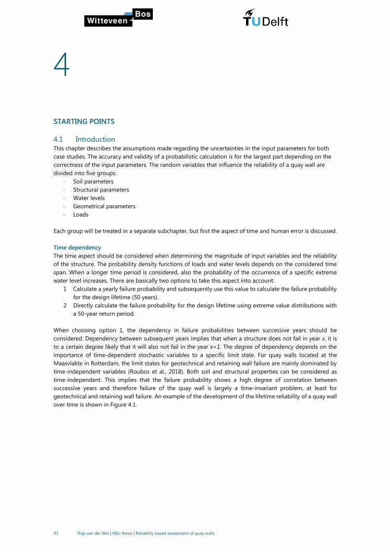
41 Thijs van der Wel | MSc thesis | Reliability based assessment of quay walls
4
STARTING POINTS
4.1 Introduction
This chapter describes the assumptions made regarding the uncertainties in the input parameters for both
case studies. The accuracy and validity of a probabilistic calculation is for the largest part depending on the
correctness of the input parameters. The random variables that influence the reliability of a quay wall are
divided into five groups:
· Soil parameters
· Structural parameters
· Water levels
· Geometrical parameters
· Loads
Each group will be treated in a separate subchapter, but first the aspect of time and human error is discussed.
Time dependency
The time aspect should be considered when determining the magnitude of input variables and the reliability
of the structure. The probability density functions of loads and water levels depends on the considered time
span. When a longer time period is considered, also the probability of the occurrence of a specific extreme
water level increases. There are basically two options to take this aspect into account:
1 Calculate a yearly failure probability and subsequently use this value to calculate the failure probability
for the design lifetime (50 years).
2 Directly calculate the failure probability for the design lifetime using extreme value distributions with
a 50-year return period.
When choosing option 1, the dependency in failure probabilities between successive years should be
considered. Dependency between subsequent years implies that when a structure does not fail in year x, it is
to a certain degree likely that it will also not fail in the year x+1. The degree of dependency depends on the
importance of time-dependent stochastic variables to a specific limit state. For quay walls located at the
Maasvlakte in Rotterdam, the limit states for geotechnical and retaining wall failure are mainly dominated by
time-independent variables (Roubos et al., 2018). Both soil and structural properties can be considered as
time-independent. This implies that the failure probability shows a high degree of correlation between
successive years and therefore failure of the quay wall is largely a time-invariant problem, at least for
geotechnical and retaining wall failure. An example of the development of the lifetime reliability of a quay wall
over time is shown in Figure 4.1.

42 Thijs van der Wel | MSc thesis | Reliability based assessment of quay walls
Figure 4.1 Development of the lifetime reliability of a quay wall. Source: Roubos et al. (2018)
In this thesis is chosen to directly calculate the 50-year failure probability by applying lifetime extreme value
distributions. In case it turns out that a load variable has negligible importance, an appropriate deterministic
value will be used. Multiple loads on the quay wall are time-dependent and therefore the frequency of
occurrence of each load should be considered. For example, the occurrence of an extreme low water
simultaneously with the maximum lifetime surcharge load seems very unlikely as both events are uncorrelated.
By applying an extreme value distribution for both parameters a very conservative load combination would be
created.
Human errors
Failure can also be caused by human errors either in the design and construction or by improper use due to
for example overloading. Because the magnitude as well as the probability of occurrence of the load or error
is unknown it is not possible to incorporate this into probabilistic design calculations. These kind of events are
classified as unidentified accidental loads in NEN-EN 1991-1-7. The code prescribes that by making a robust
design, failure caused by this type of loads is prevented sufficiently.
4.2 Soil parameter uncertainties
The uncertainty in a parameter is described by its Coefficient Of Variation (COV). The main sources of
uncertainty in a soil parameter are (Baecher & Christian, 2003):
· Measurement uncertainty
· The quality of measurements depends on the precision of the measurement devices, the type of test
and the skills and experience of the people performing the test.
· Spatial variation
· This type of uncertainty is related to the randomness that exist in nature and cannot be reduced.
· Transformation uncertainty
· Soil properties are often not directly measured but derived using empirical correlations or
transformation models. These models contain also uncertainty.
· Statistical uncertainty
· Soil parameters are often derived from limited soil investigation resulting in a certain degree of
statistical uncertainty
Ideally, the uncertainty in a local soil parameter is determined from a statistical analysis on a large set of in-
situ measurements and lab tests. However, this is very time consuming and requires a sufficient amount of in-
situ tests. For this reasons the COV-values will be taken from literature. Table 4.1 gives an overview of values
described by several sources: NEN-9997, JCSS (2006), Wolters (2012), Griffiths and Fenton (2007) and Schneider
and Schneider (2013). As Table 4.1 indicates, there does not exist one single value that is applicable in every
case. The COV-values differs per soil type, per soil parameter -and per location. In principle, all soil properties
are normally distributed. However, applying this in a reliability analysis can result in negative values for certain
parameters, which is physically impossible. Therefore the log-normal distribution is used for cohesion and
stiffness. If needed, for all other parameters a truncated normal distribution is applied to increase the
robustness of the FORM analysis. The boundaries are then chosen wide enough not influence on the shape of
the distribution.

43 Thijs van der Wel | MSc thesis | Reliability based assessment of quay walls
Table 4.1 Overview on COV-values in literature
Parameter Symbol Distribution NEN
9997 JCSS
Griffiths &
Fenton Wolters
Schneider
&
Schneider
Density 𝛾 Normal 0.05 0.05 - 0.1 0 - 0.1 0.05 0.01 - 0.1
Friction
angle 𝜑 Normal 0.10 0.1 - 0.2
0.02 - 0.05
(sand) 0.2
0.05 -
0.15
Cohesion 𝑐 Lognormal 0.20 0.1 - 0.5 0.1 - 0.35 0.8 0.3 - 0.5
Stiffness 𝐸 Lognormal 0.10 0.2 - 1.0 0.30 0.2 - 0.7
Stiffness
parameter 𝑚 Normal 0.2
Interface
strength
𝑅𝑖𝑛𝑡𝑒𝑟 Normal 0.2
Dilatancy
angle Ψ Normal 0.2
As one can notice, in the study of Wolters also m, 𝑅𝑖𝑛𝑡𝑒𝑟 and Ψ at first were chosen as random variables.
However, after the sensitivity analysis they appeared to have negligible influence in the limit state function of
soil mechanical failure. For this reason they are considered deterministic throughout this thesis.
Spatial averaging and spatial variability
It is important to know whether a given COV value of a certain soil property represents the variation in a certain
point in space or the variation in the local average of a layer. For the reliability of quay walls, two aspect are of
importance for choosing the COV:
- Spatial averaging (depending on the considered failure mode)
- Inherent spatial variability
Spatial averaging
For several failure modes not the variation in a certain point is of interest, but instead the variation of the mean
value of a whole layer. Whether mean values or local point values are of importance for a limit state depends
on the ratio between the scale of fluctuation𝜃 and the domain of influence D (Hicks, 2013). The scale of
fluctuation is a measure of the distance over which property values are significantly correlated. Due to the
geological process of layer deposition, the scale of fluctuation in the horizontal direction is often much larger
than in the vertical direction. The scale of fluctuation in vertical direction 𝜃𝑦 is in the order of 2 meter. The scale
of fluctuation in the horizontal direction is in the order of 50m. Although this is definitely not a constant value.
It depends on the way in which a deposition is formed and it also varies for every parameter (Schneider &
Schneider, 2013).
The domain of influence differs for each limit state. When the ratio 𝜃/D is very small, as for a large slip circle,
the failure plane cuts through entire soil layers and the mean averaged property values of soil are of
importance and therefore also the variation of the mean averaged properties. Mean averaged values have a
much narrower distribution (lower COV) than local point values as illustrated in Figure 4.2.

44 Thijs van der Wel | MSc thesis | Reliability based assessment of quay walls
Figure 4.2 Probability density function of local point value vs layer averaged value
On the other hand, a sliding plane has the tendency to follow the path of the least resistance, which partly
cancels out the argument just mentioned.
When the domain of influence is small with respect to the scale of fluctuation, the use of point variations is
more appropriate. For instance for the bearing capacity of a soil under a pile. For the failure of the wall in
bending, the domain of influence is large as the load on the wall is caused by multiple soil layers, whereas the
vertical scale of fluctuation is small. Also the concrete superstructure and the combi-wall have a large
distribution capacity which causes load spreading in the horizontal direction. For this reason, the variation in
mean average values is applicable.
Interpretation of COV-values of NEN9997 and conclusion
The background and interpretation of the values for the COV given in the NEN9997 are not described in the
code itself and therefore some debate on this values has been going on. It is known that these values are
based on results from soil investigations in The Netherlands combined with expert judgement. The CUR
committee C135 has elaborated this values and stated that the values given in NEN9997 can be interpreted as
locally layer averaged values (CUR-C135, 2008) which can be used when there is insufficient data from site
investigation.
Therefore these values will be used in this thesis. Only the COV for the stiffness is slightly raised to 0.30 as a
value of 0.10 is rather low compared to other values given in literature (see Table 4.1). The importance and
uncertainty of the stress dependency factor m, the interface strength and the dilatancy angle is unknown. In
this thesis they are considered deterministic for the sake of simplicity.
An overview on the used values is given in Table 4.2.
Table 4.2 Statistical properties
Parameter Symbol Distribution COV
Density 𝛾 Normal 0.05
Friction angle 𝜑 Normal 0.10
Cohesion 𝑐 Lognormal 0.20
Stiffness 𝐸 Lognormal 0.30
Stress-level dependency of stiffness 𝑚 Deterministic -
Interface strength 𝑅𝑖𝑛𝑡𝑒𝑟 Deterministic -
Dilatancy angle Ψ Deterministic -
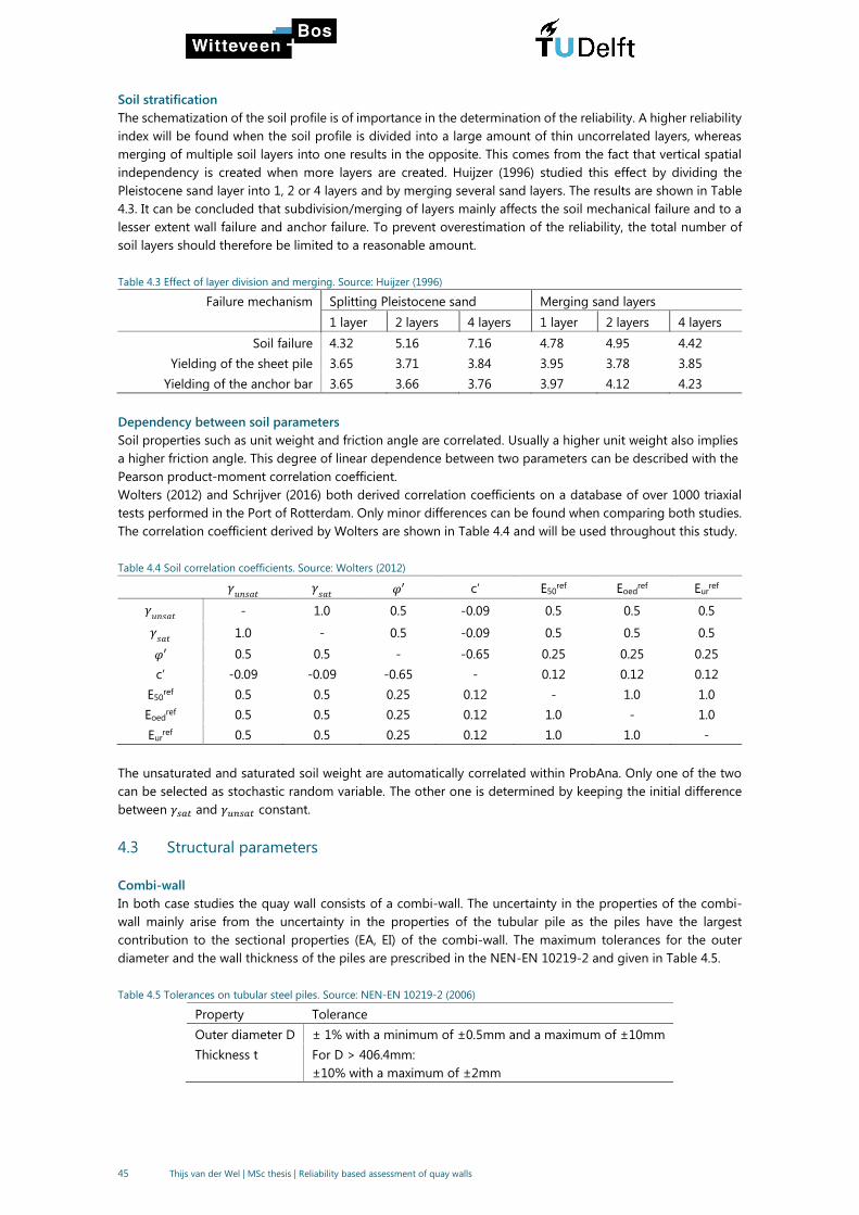
45 Thijs van der Wel | MSc thesis | Reliability based assessment of quay walls
Soil stratification
The schematization of the soil profile is of importance in the determination of the reliability. A higher reliability
index will be found when the soil profile is divided into a large amount of thin uncorrelated layers, whereas
merging of multiple soil layers into one results in the opposite. This comes from the fact that vertical spatial
independency is created when more layers are created. Huijzer (1996) studied this effect by dividing the
Pleistocene sand layer into 1, 2 or 4 layers and by merging several sand layers. The results are shown in Table
4.3. It can be concluded that subdivision/merging of layers mainly affects the soil mechanical failure and to a
lesser extent wall failure and anchor failure. To prevent overestimation of the reliability, the total number of
soil layers should therefore be limited to a reasonable amount.
Table 4.3 Effect of layer division and merging. Source: Huijzer (1996)
Failure mechanism Splitting Pleistocene sand Merging sand layers
1 layer 2 layers 4 layers 1 layer 2 layers 4 layers
Soil failure 4.32 5.16 7.16 4.78 4.95 4.42
Yielding of the sheet pile 3.65 3.71 3.84 3.95 3.78 3.85
Yielding of the anchor bar 3.65 3.66 3.76 3.97 4.12 4.23
Dependency between soil parameters
Soil properties such as unit weight and friction angle are correlated. Usually a higher unit weight also implies
a higher friction angle. This degree of linear dependence between two parameters can be described with the
Pearson product-moment correlation coefficient.
Wolters (2012) and Schrijver (2016) both derived correlation coefficients on a database of over 1000 triaxial
tests performed in the Port of Rotterdam. Only minor differences can be found when comparing both studies.
The correlation coefficient derived by Wolters are shown in Table 4.4 and will be used throughout this study.
Table 4.4 Soil correlation coefficients. Source: Wolters (2012)
𝛾𝑢𝑛𝑠𝑎𝑡
𝛾𝑠𝑎𝑡
𝜑′ c’ E50ref Eoed
ref Eurref
𝛾𝑢𝑛𝑠𝑎𝑡
- 1.0 0.5 -0.09 0.5 0.5 0.5
𝛾𝑠𝑎𝑡
1.0 - 0.5 -0.09 0.5 0.5 0.5
𝜑′ 0.5 0.5 - -0.65 0.25 0.25 0.25
c’ -0.09 -0.09 -0.65 - 0.12 0.12 0.12
E50ref 0.5 0.5 0.25 0.12 - 1.0 1.0
Eoedref 0.5 0.5 0.25 0.12 1.0 - 1.0
Eurref 0.5 0.5 0.25 0.12 1.0 1.0 -
The unsaturated and saturated soil weight are automatically correlated within ProbAna. Only one of the two
can be selected as stochastic random variable. The other one is determined by keeping the initial difference
between 𝛾𝑠𝑎𝑡 and 𝛾𝑢𝑛𝑠𝑎𝑡 constant.
4.3 Structural parameters
Combi-wall
In both case studies the quay wall consists of a combi-wall. The uncertainty in the properties of the combi-
wall mainly arise from the uncertainty in the properties of the tubular pile as the piles have the largest
contribution to the sectional properties (EA, EI) of the combi-wall. The maximum tolerances for the outer
diameter and the wall thickness of the piles are prescribed in the NEN-EN 10219-2 and given in Table 4.5.
Table 4.5 Tolerances on tubular steel piles. Source: NEN-EN 10219-2 (2006)
Property Tolerance
Outer diameter D ± 1% with a minimum of ±0.5mm and a maximum of ±10mm
Thickness t For D > 406.4mm:
±10% with a maximum of ±2mm

46 Thijs van der Wel | MSc thesis | Reliability based assessment of quay walls
The tubular piles in both case studies have a diameter of 1420mm. This means that the diameter has a
maximum deviation of 10mm. It is assumed that the diameter is uniformly distributed. The wall thickness
deviates with a maximum of 10%, and is assumed to be normally distributed with a COV of 0.03, With this
value the PDF is for 99.9% within the boundaries of the thickness tolerances of NEN-EN 10219-2 (Figure 4.3).
Figure 4.3 PDF of wall thickness with COV of 0.03 (the red lines are the limits for the thickness tolerances given in NEN-EN10219-6)
Uncertainties in the Young’s modulus and the yield strength are taken from the Joint Committee on Structural
Safety (2006).The test results of Peters et al. (2017) on the yield strength confirm the COV of 0.07. It also shows
that values lower than 0.8 times the nominal value do not appear.
The thickness of the intermediate sheet piles can also deviate by a maximum of 6% but the contribution of the
intermediate sheet piles to the sectional properties of the combi-wall can in practice be neglected. Due to the
large stiffness difference between the tubular piles and the sheet pile, horizontal soil arches develop and all
the load is transferred to the tubular piles. Therefore, the sheet pile properties are not taken into account here.
Table 4.6 COV of the material properties of steel tubular piles
Parameter Symbol Distribution COV
Yield stress 𝑓𝑦 Normal 0.07
Young’s modulus E Normal 0.03
Wall thickness t Normal 0.03
Pile diameter D Uniform +/-10mm
With this information the coefficient of variation of the sectional properties of the combi-wall can be
determined with a Monte Carlo simulation in Python (Appendix C). The input required in Plaxis is:
- The axial stiffness: EA [kN/m}
- The bending stiffness: EI [kNm2/m]
- Weight per meter length: w [kN/m/m]
Whereas in the LSF for failure of the wall the following properties are required:
- Elastic section modulus Wel
- Cross-sectional area A
- Yield strength fy
The coefficients of variation obtained with the Monte Carlo simulation are given in Table 4.7.
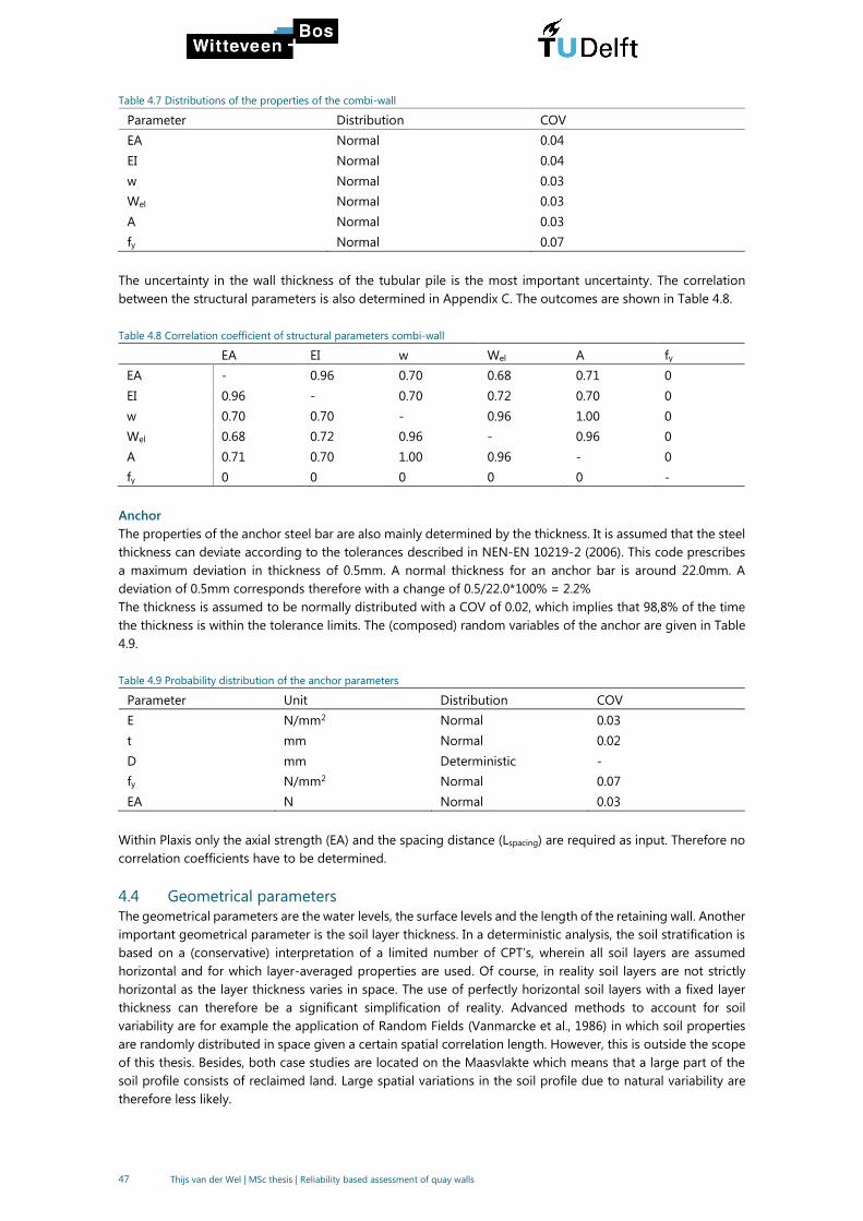
47 Thijs van der Wel | MSc thesis | Reliability based assessment of quay walls
Table 4.7 Distributions of the properties of the combi-wall
Parameter Distribution COV
EA Normal 0.04
EI Normal 0.04
w Normal 0.03
Wel Normal 0.03
A Normal 0.03
fy Normal 0.07
The uncertainty in the wall thickness of the tubular pile is the most important uncertainty. The correlation
between the structural parameters is also determined in Appendix C. The outcomes are shown in Table 4.8.
Table 4.8 Correlation coefficient of structural parameters combi-wall
EA EI w Wel A fy
EA - 0.96 0.70 0.68 0.71 0
EI 0.96 - 0.70 0.72 0.70 0
w 0.70 0.70 - 0.96 1.00 0
Wel 0.68 0.72 0.96 - 0.96 0
A 0.71 0.70 1.00 0.96 - 0
fy 0 0 0 0 0 -
Anchor
The properties of the anchor steel bar are also mainly determined by the thickness. It is assumed that the steel
thickness can deviate according to the tolerances described in NEN-EN 10219-2 (2006). This code prescribes
a maximum deviation in thickness of 0.5mm. A normal thickness for an anchor bar is around 22.0mm. A
deviation of 0.5mm corresponds therefore with a change of 0.5/22.0*100% = 2.2%
The thickness is assumed to be normally distributed with a COV of 0.02, which implies that 98,8% of the time
the thickness is within the tolerance limits. The (composed) random variables of the anchor are given in Table
4.9.
Table 4.9 Probability distribution of the anchor parameters
Parameter Unit Distribution COV
E N/mm2 Normal 0.03
t mm Normal 0.02
D mm Deterministic -
fy N/mm2 Normal 0.07
EA N Normal 0.03
Within Plaxis only the axial strength (EA) and the spacing distance (Lspacing) are required as input. Therefore no
correlation coefficients have to be determined.
4.4 Geometrical parameters
The geometrical parameters are the water levels, the surface levels and the length of the retaining wall. Another
important geometrical parameter is the soil layer thickness. In a deterministic analysis, the soil stratification is
based on a (conservative) interpretation of a limited number of CPT’s, wherein all soil layers are assumed
horizontal and for which layer-averaged properties are used. Of course, in reality soil layers are not strictly
horizontal as the layer thickness varies in space. The use of perfectly horizontal soil layers with a fixed layer
thickness can therefore be a significant simplification of reality. Advanced methods to account for soil
variability are for example the application of Random Fields (Vanmarcke et al., 1986) in which soil properties
are randomly distributed in space given a certain spatial correlation length. However, this is outside the scope
of this thesis. Besides, both case studies are located on the Maasvlakte which means that a large part of the
soil profile consists of reclaimed land. Large spatial variations in the soil profile due to natural variability are
therefore less likely.
48 Thijs van der Wel | MSc thesis | Reliability based assessment of quay walls
Water levels
The Port of Rotterdam is in direct connection with the open sea. Therefore the tide is influencing the water
levels within the port. The normative load case for a quay wall is generally a low outer water level and a high
ground water level. Especially the difference between these two water levels is of importance. The degree of
correlation between both water levels depends on the presence and functioning of a drainage system, the
permeability of the wall and the permeability of the soil.
Surface levels
The surface level on the landside is normally known with high accuracy and does not deviate much because
very often the surface is paved up till the edge of the wall.
The bottom level on the water side of the wall is much more uncertain due the inaccuracies of the dredging
equipment and the placement of the bed protection. In case no bed protection is applied scour holes are a
large threat.
Length retaining wall
The length of the sheet pile or the tubular piles can deviate from its design specifications due to for example
installation problems after which the piles are not installed to the predefined depth. This kind of uncertainty
will not be taken into account here.
4.5 Load parameters
Next to the load imposed by the soil and the water level difference also other loads are active on the structure.
Loads that are of importance for a quay wall in the Rotterdam region are:
· Mooring loads
· Berthing loads
· Surcharge loads (Coal piles, container stacks etc.)
· Crane loads
· Temperature loads
· Wind loads
· Vessel collision
The magnitude and distribution of variables describing the load on a quay wall are largely site-specific, whereas
each type of load also has different characteristics. Therefore, they are described separately in each case study.

49 Thijs van der Wel | MSc thesis | Reliability based assessment of quay walls
5
CASE STUDY 1: DOUBLE ANCHORED COMBI-WALL
5.1 Introduction
The first case study considers a quay wall constructed in the Port of Rotterdam near a storage location for
LNG. This quay wall is constructed in 2016 and is designed in accordance to RC3. The structure consist of a
combi-wall with concrete cap. The combi-wall is anchored by two grout anchors in the tubular steel piles of
the combi-wall and has a retaining height of approximately 20m. An overview of original design model is
shown in Figure 5.1.
The goal of the first part of this case study is to get familiar with the use of ProbAna and Plaxis. The problem
is therefore partly simplified by reducing the amount of soil layers and the amount of construction stages. Also
only the load case that was normative for both the anchor and the wall is considered.
The following aspects are considered in this case study:
- The difference in results between calculations using correlated or uncorrelated variables
- The influence of the uncertainty in structural properties on the reliability for the considered limit state.
(structural properties cannot be inserted as stochastic in ProbAna)
- The applicability of FORM for the three considered failure mechanisms
- Where possible a comparison with the maximum allowed reliability index prescribed by guidelines
- The influence of time-dependant variables
The second part of the case study is focussed on the derivation of partial factors and the evaluation of an
critical limit state.
Figure 5.1 Original design model of the quay wall
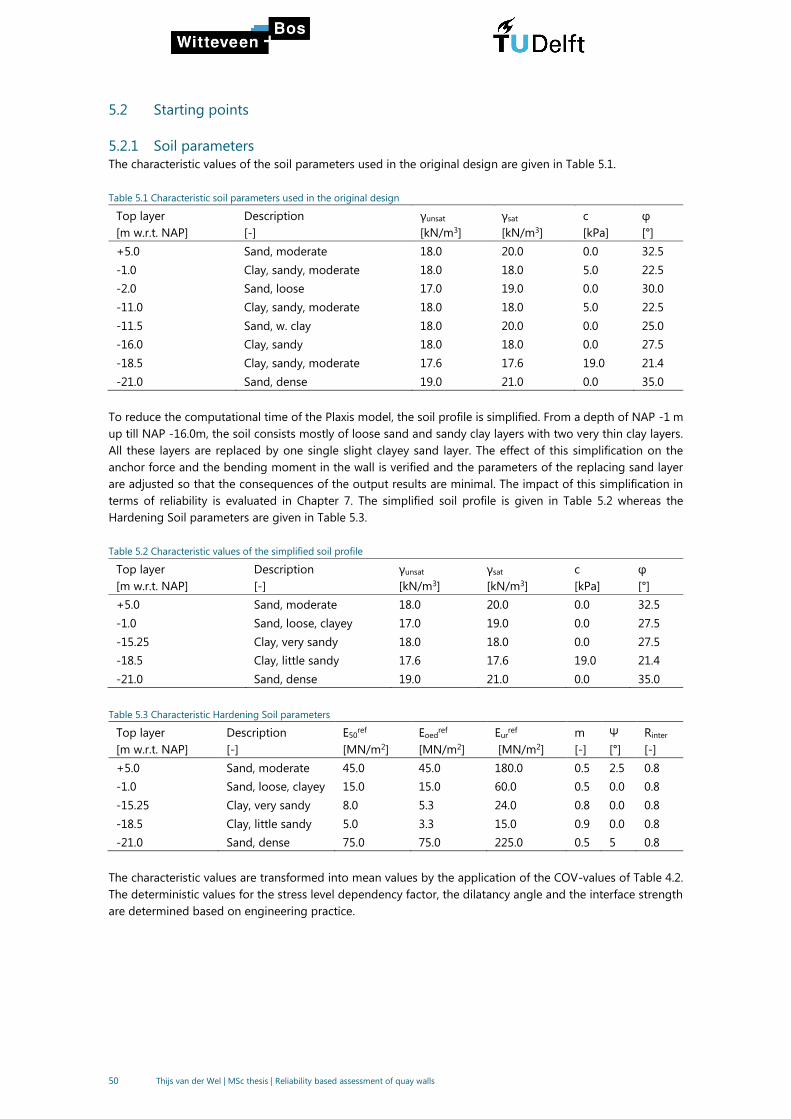
50 Thijs van der Wel | MSc thesis | Reliability based assessment of quay walls
5.2 Starting points
5.2.1 Soil parameters
The characteristic values of the soil parameters used in the original design are given in Table 5.1.
Table 5.1 Characteristic soil parameters used in the original design
Top layer
[m w.r.t. NAP]
Description
[-]
γunsat
[kN/m3]
γsat
[kN/m3]
c
[kPa]
φ
[°]
+5.0 Sand, moderate 18.0 20.0 0.0 32.5
-1.0 Clay, sandy, moderate 18.0 18.0 5.0 22.5
-2.0 Sand, loose 17.0 19.0 0.0 30.0
-11.0 Clay, sandy, moderate 18.0 18.0 5.0 22.5
-11.5 Sand, w. clay 18.0 20.0 0.0 25.0
-16.0 Clay, sandy 18.0 18.0 0.0 27.5
-18.5 Clay, sandy, moderate 17.6 17.6 19.0 21.4
-21.0 Sand, dense 19.0 21.0 0.0 35.0
To reduce the computational time of the Plaxis model, the soil profile is simplified. From a depth of NAP -1 m
up till NAP -16.0m, the soil consists mostly of loose sand and sandy clay layers with two very thin clay layers.
All these layers are replaced by one single slight clayey sand layer. The effect of this simplification on the
anchor force and the bending moment in the wall is verified and the parameters of the replacing sand layer
are adjusted so that the consequences of the output results are minimal. The impact of this simplification in
terms of reliability is evaluated in Chapter 7. The simplified soil profile is given in Table 5.2 whereas the
Hardening Soil parameters are given in Table 5.3.
Table 5.2 Characteristic values of the simplified soil profile
Top layer
[m w.r.t. NAP]
Description
[-]
γunsat
[kN/m3]
γsat
[kN/m3]
c
[kPa]
φ
[°]
+5.0 Sand, moderate 18.0 20.0 0.0 32.5
-1.0 Sand, loose, clayey 17.0 19.0 0.0 27.5
-15.25 Clay, very sandy 18.0 18.0 0.0 27.5
-18.5 Clay, little sandy 17.6 17.6 19.0 21.4
-21.0 Sand, dense 19.0 21.0 0.0 35.0
Table 5.3 Characteristic Hardening Soil parameters
Top layer
[m w.r.t. NAP]
Description
[-]
E50ref
[MN/m2]
Eoedref
[MN/m2]
Eurref
[MN/m2]
m
[-]
Ψ
[°]
Rinter
[-]
+5.0 Sand, moderate 45.0 45.0 180.0 0.5 2.5 0.8
-1.0 Sand, loose, clayey 15.0 15.0 60.0 0.5 0.0 0.8
-15.25 Clay, very sandy 8.0 5.3 24.0 0.8 0.0 0.8
-18.5 Clay, little sandy 5.0 3.3 15.0 0.9 0.0 0.8
-21.0 Sand, dense 75.0 75.0 225.0 0.5 5 0.8
The characteristic values are transformed into mean values by the application of the COV-values of Table 4.2.
The deterministic values for the stress level dependency factor, the dilatancy angle and the interface strength
are determined based on engineering practice.

51 Thijs van der Wel | MSc thesis | Reliability based assessment of quay walls
Depending on whether it is a load parameter or a strength parameter the mean value is determined in the
following way:
𝜇𝑖 =𝑋𝑖,𝑘
1 ± 1.64𝐶𝑂𝑉𝑖(5.1)
In the case of log-normally distributed variables the mean value can be determined by:
𝜇𝑋𝑖 =𝑋𝑘,𝑖√1 + 𝐶𝑂𝑉𝑖
2
exp(−1.645√ln(1 + 𝐶𝑂𝑉𝑖2))
(5.2)
The values for volumetric weight are already mean values and are therefore not changed. For some other
parameters the outcomes are slightly adjusted to avoid physically unrealistic values.
The expected soil parameters are given in Table 5.4 and Table 5.5
Table 5.4 Mean values of the soil parameters
Top layer
[m w.r.t. NAP]
Description
[-]
γunsat
[kN/m3]
γsat
[kN/m3]
c’
[kPa]
φ’
[°]
+5.0 Sand, moderate 18.0 20.0 0.0 38.9
-1.0 Sand, loose, clayey 17.0 19.0 0.0 32.9
-15.25 Clay, very sandy 18.0 18.0 0.0 32.9
-18.5 Clay, little sandy 17.6 17.6 28.3 25.6
-21.0 Sand, dense 19.0 21.0 0.0 40.0
Table 5.5 Mean values of the HS parameters
Top layer
[m w.r.t. NAP]
Description
[-]
E50ref
[MN/m2]
Eoedref
[MN/m2]
Eurref
[MN/m2]
m
[-]
Ψ
[°]
Rinter
[-]
+5.0 Sand, moderate 45 45 135 0.5 2.5 0.8
-1.0 Sand, loose, clayey 30 30 90 0.5 0.0 0.8
-15.25 Clay, very sandy 16 10 48 0.8 0.0 0.8
-18.5 Clay, little sandy 10 6 30 0.9 0.0 0.8
-21.0 Sand, dense 70 70 210 0.5 5 0.8
Figure 5.2 Schematization of the quay wall
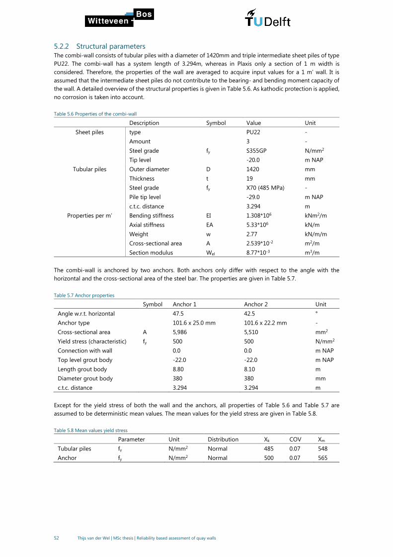
52 Thijs van der Wel | MSc thesis | Reliability based assessment of quay walls
5.2.2 Structural parameters
The combi-wall consists of tubular piles with a diameter of 1420mm and triple intermediate sheet piles of type
PU22. The combi-wall has a system length of 3.294m, whereas in Plaxis only a section of 1 m width is
considered. Therefore, the properties of the wall are averaged to acquire input values for a 1 m’ wall. It is
assumed that the intermediate sheet piles do not contribute to the bearing- and bending moment capacity of
the wall. A detailed overview of the structural properties is given in Table 5.6. As kathodic protection is applied,
no corrosion is taken into account.
Table 5.6 Properties of the combi-wall
Description Symbol Value Unit
Sheet piles type PU22 -
Amount 3 -
Steel grade fy S355GP N/mm2
Tip level -20.0 m NAP
Tubular piles Outer diameter D 1420 mm
Thickness t 19 mm
Steel grade fy X70 (485 MPa) -
Pile tip level -29.0 m NAP
c.t.c. distance 3.294 m
Properties per m’ Bending stiffness EI 1.308*106 kNm2/m
Axial stiffness EA 5.33*106 kN/m
Weight w 2.77 kN/m/m
Cross-sectional area A 2.539*10-2 m2/m
Section modulus Wel 8.77*10-3 m3/m
The combi-wall is anchored by two anchors. Both anchors only differ with respect to the angle with the
horizontal and the cross-sectional area of the steel bar. The properties are given in Table 5.7.
Table 5.7 Anchor properties
Symbol Anchor 1 Anchor 2 Unit
Angle w.r.t. horizontal 47.5 42.5 °
Anchor type 101.6 x 25.0 mm 101.6 x 22.2 mm -
Cross-sectional area A 5,986 5,510 mm2
Yield stress (characteristic) fy 500 500 N/mm2
Connection with wall 0.0 0.0 m NAP
Top level grout body -22.0 -22.0 m NAP
Length grout body 8.80 8.10 m
Diameter grout body 380 380 mm
c.t.c. distance 3.294 3.294 m
Except for the yield stress of both the wall and the anchors, all properties of Table 5.6 and Table 5.7 are
assumed to be deterministic mean values. The mean values for the yield stress are given in Table 5.8.
Table 5.8 Mean values yield stress
Parameter Unit Distribution Xk COV Xm
Tubular piles fy N/mm2 Normal 485 0.07 548
Anchor fy N/mm2 Normal 500 0.07 565

53 Thijs van der Wel | MSc thesis | Reliability based assessment of quay walls
5.2.3 Construction stages and meshing
The computation time for each LSFE depends largely on the amount of construction stages and the coarseness
of the mesh. A balance should be found between accuracy and computational time.
The construction stages for this project are:
1 Gravity loading
2 Installation of the combi-wall
3 Excavating to NAP +0.0m
4 Installation and prestressing of the grout anchors
5 Excavation until construction depth of NAP-15.25m
6 Load case
7 (safety phase)
The applied mesh size in this model is medium, resulting in the mesh plot shown in Figure 5.3.
Figure 5.3 Connectivity plot
5.2.4 Loads, water levels and geometry
Due to the time limitations, the reliability of the quay wall is only determined for one load case, which is the
normative load case in the original design. This concerns the load combination with a surcharge load of 40
kPa and a bollard load of 28kN/m’.
For the time-dependant variables, the applied values are representative for the design lifetime.
Permanent loads
The considered permanent loads are the weight of the concrete cap beam (400 kN/m) and the weight of the
bottom protection (10kPa).
Variable loads
The considered variable loads are the surcharge load of 40 kPa next to the quay wall and the bollard load of
28 kN at a level of NAP +1.7m.
Geometry
The ground surface level is at NAP +5.0m, which can be determined with high accuracy and is therefore
considered deterministic. The bottom level is assumed at the design depth of NAP-15.25m. The occurrence of
scour holes is prevented by a bed protection. Within the calculation of the design depth, the dredging and
placement tolerances are already taken into account. Also, the bottom level is taken as deterministic in this
case study.

54 Thijs van der Wel | MSc thesis | Reliability based assessment of quay walls
Water levels
For the first calculations, only the soil parameters are considered as random variables. Therefore,
deterministic values for the outer water level and ground water level are determined here.
The difference between the outer water level (OWL) and the ground water level (GWL) is the most important
water load on the quay wall. In the final calculation phase in Plaxis the OWL is chosen in accordance to CUR211.
Table 5.9 Fundamental water pressure difference ∆h with drainage. Source: CUR211 (2013)
Water level fluctuations Soil conditions OWL GWL ∆hmin
Minor - MLW hdrainage + 0.3m > 0.5m
Major (rivers) - OLW/OLR hdrainage + 0.3m > 0.5m
Tidal conditions - LLWS hdrainage + 0.3m > 0.5m
In case of a load combination where the water level difference is not the dominant load, which is the case here,
the OWL is taken as Low Low water Spring (LLWS), which is the mean of the lowest spring tide level of every
month over 5 years. For this case holds: LLWS = NAP -0.84m.
The quay wall is equipped with a drainage system at LLWS. In case of a working drainage system, the GWL
should be the maximum value of (hdrainage +0.3m; OWL + 0.5m). The second value is normative, resulting in a
ground water level of NAP-0.34m.
It should be noted that the occurrence of extreme low water levels should be considered in a separate
accidental load case, which turned out not to be the normative load case for the bending moment of the wall.
Considering both extreme loads and extreme water levels in one load case would be very unrealistic, the two
loads are uncorrelated and therefore the probability that they occur simultaneously is very small.
During the construction stages, the ground water potential in all layers is taken at NAP +0.07m. In the final
calculation phase, the ground water potential in the loose sand layer on the land side is set to NAP-0.34m,
whereas the potential in the (deep) dense sand layer is set equal to the outer water level (=LLWS). The two
thin clay layers are set on interpolation. The modelling of the groundwater pressures is depicted in Figure 5.4.
Figure 5.4 Modelling of the ground water pressures
As almost the complete soil profile consists of sand layers and sandy clay layers, all calculations in this case
study are performed assuming drained conditions. The present clay layers are thin, which also means they can
drain relatively quickly. Therefore, it is expected that this simplification has negligible influence on the
outcomes.
5.3 LS1: Yielding of the combi-wall
Firstly, the yielding of the sheet pile wall is considered. The general equation for the limit state of the yielding
of the combi-wall was already discussed in chapter 5.2.1.
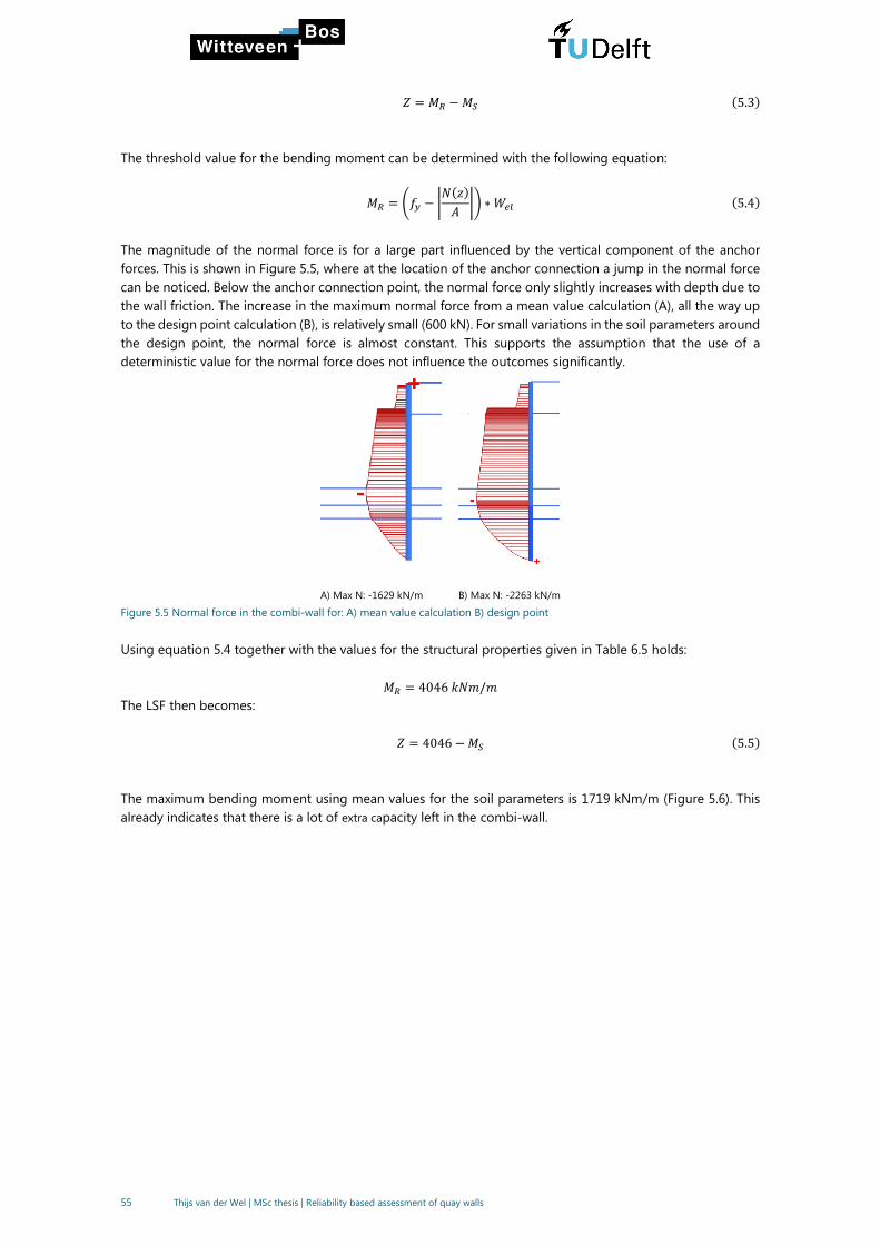
55 Thijs van der Wel | MSc thesis | Reliability based assessment of quay walls
𝑍 = 𝑀𝑅 −𝑀𝑆 (5.3)
The threshold value for the bending moment can be determined with the following equation:
𝑀𝑅 = (𝑓𝑦 − |𝑁(𝑧)
𝐴|) ∗ 𝑊𝑒𝑙 (5.4)
The magnitude of the normal force is for a large part influenced by the vertical component of the anchor
forces. This is shown in Figure 5.5, where at the location of the anchor connection a jump in the normal force
can be noticed. Below the anchor connection point, the normal force only slightly increases with depth due to
the wall friction. The increase in the maximum normal force from a mean value calculation (A), all the way up
to the design point calculation (B), is relatively small (600 kN). For small variations in the soil parameters around
the design point, the normal force is almost constant. This supports the assumption that the use of a
deterministic value for the normal force does not influence the outcomes significantly.
A) Max N: -1629 kN/m B) Max N: -2263 kN/m
Figure 5.5 Normal force in the combi-wall for: A) mean value calculation B) design point
Using equation 5.4 together with the values for the structural properties given in Table 6.5 holds:
𝑀𝑅 = 4046𝑘𝑁𝑚/𝑚
The LSF then becomes:
𝑍 = 4046 −𝑀𝑆 (5.5)
The maximum bending moment using mean values for the soil parameters is 1719 kNm/m (Figure 5.6). This
already indicates that there is a lot of extra capacity left in the combi-wall.

56 Thijs van der Wel | MSc thesis | Reliability based assessment of quay walls
Figure 5.6 Bending moment distribution with a mean value calculation
5.3.1 FORM sensitivity analysis
To determine the most relevant parameters, a sensitivity analysis is carried out with uncorrelated parameters.
In this way, a better insight is gathered into the most important parameters, without the effect that a parameter
is increased only due to its correlation with another parameter and not due to its own influence.
Only the soil parameters are taken as variables in this first case study. For every layer the volumetric weight,
the friction angle and the stiffness are considered as stochastic, except for the clay layers, in which the
volumetric weight is not considered due to the small size of these layers and the relatively small uncertainty
of this property.
When considering the results of Figure 5.7, it can be clearly concluded that the friction angle is the most
dominant soil parameter in this case. This can be explained by the fact that the active lateral soil pressures
increase when the friction angle decreases, resulting in a larger load on the wall. Besides, the passive resistance
of the soil decreases when the friction angle decreases. The friction angle of the loose sand layer is the most
dominant parameter. This was also expected given the vertical extent of this layer and its position covering
the entire free span length of the wall between the anchor and fixation in the soil. The soil stiffness seems to
have only little influence in this case.
Figure 5.7 Importance factors wall failure, uncorrelated
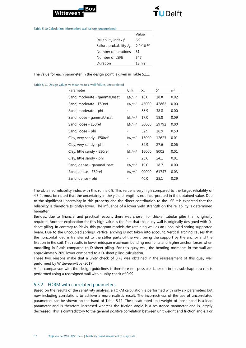
57 Thijs van der Wel | MSc thesis | Reliability based assessment of quay walls
Table 5.10 Calculation information, wall failure, uncorrelated
Value
Reliability index β 6.9
Failure probability 𝑃𝑓 2.2*10-12
Number of iterations 31
Number of LSFE 547
Duration 18 hrs
The value for each parameter in the design point is given in Table 5.11.
Table 5.11 Design values vs mean values, wall failure, uncorrelated
Parameter Unit Xm X* α2
Sand, moderate - gammaUnsat kN/m3 18.0 18.8 0.02
Sand, moderate - E50ref kN/m2 45000 42862 0.00
Sand, moderate - phi ᵒ 38.9 38.8 0.00
Sand, loose - gammaUnsat kN/m3 17.0 18.8 0.09
Sand, loose - E50ref kN/m2 30000 29792 0.00
Sand, loose - phi ᵒ 32.9 16.9 0.50
Clay, very sandy - E50ref kN/m2 16000 12623 0.01
Clay, very sandy - phi ᵒ 32.9 27.6 0.06
Clay, little sandy - E50ref kN/m2 16000 8002 0.01
Clay, little sandy - phi ᵒ 25.6 24.1 0.01
Sand, dense - gammaUnsat kN/m3 19.0 18.7 0.00
Sand, dense - E50ref kN/m2 90000 61747 0.03
Sand, dense - phi ᵒ 40.0 25.1 0.29
The obtained reliability index with this run is 6.9. This value is very high compared to the target reliability of
4.3. It must be noted that the uncertainty in the yield strength is not incorporated in the obtained value. Due
to the significant uncertainty in this property and the direct contribution to the LSF it is expected that the
reliability is therefore (slightly) lower. The influence of a lower yield strength on the reliability is determined
hereafter.
Besides, due to financial and practical reasons there was chosen for thicker tubular piles than originally
required. Another explanation for this high value is the fact that this quay wall is originally designed with D-
sheet piling. In contrary to Plaxis, this program models the retaining wall as an uncoupled spring supported
beam. Due to the uncoupled springs, vertical arching is not taken into account. Vertical arching causes that
the horizontal load is transferred to the stiffer parts of the wall, being the support by the anchor and the
fixation in the soil. This results in lower midspan maximum bending moments and higher anchor forces when
modelling in Plaxis compared to D-sheet piling. For this quay wall, the bending moments in the wall are
approximately 20% lower compared to a D-sheet piling calculation.
These two reasons make that a unity check of 0.78 was obtained in the reassessment of this quay wall
performed by Witteveen+Bos (2017).
A fair comparison with the design guidelines is therefore not possible. Later on in this subchapter, a run is
performed using a redesigned wall with a unity check of 0.99.
5.3.2 FORM with correlated parameters
Based on the results of the sensitivity analysis, a FORM calculation is performed with only six parameters but
now including correlations to achieve a more realistic result. The incorrectness of the use of uncorrelated
parameters can be shown on the hand of Table 5.11. The unsaturated unit weight of loose sand is a load
parameter and is therefore increased whereas the friction angle is a resistance parameter and is largely
decreased. This is contradictory to the general positive correlation between unit weight and friction angle. For

58 Thijs van der Wel | MSc thesis | Reliability based assessment of quay walls
this kind of reasons it can be expected that the use of correlated parameters would result in a lower failure
probability.
The performed calculation with correlated parameters did not converge within the 30 iterations that were set
as a limit. By analysing the results of this run, the errors were reasonably close to their tolerances and therefore
the results are accepted (Table 5.12).
The reliability index β found is 7.4, which is considerably higher than the value of 6.9 found with the
uncorrelated parameters.
Table 5.12 Calculation results, wall failure, correlated
Value
Reliability index β 7.4
Failure probability 𝑃𝑓 6.0*10-14
Number of iterations 31
Number of LSFE 315
Duration 30 hrs
Absolute error after 30 iterations: 0.09 Tolerance: 0.05
Relative error after 30 iterations: 0.01 Tolerance: 0.05
Residual error after 30 iterations: 0.28 Tolerance: 0.05
Constraint error after 30 iterations: 3.5 kNm Tolerance: 20
The obtained importance factors are compared to the importance factors of the run with uncorrelated
parameters (Figure 5.8). It can be seen that the differences in general are relatively small. Especially a significant
change in the importance of the stiffness of the dense sand layer can be noticed. This change can be partly
clarified by the correlation with the friction angle, but this is only a weak correlation (0.25) and therefore it
does not fully explain this change. Apparently due to the reduction in the number of stochastic variables and
the redistribution of importance, more importance is taken by the stiffness of the dense sand layer.
Another large relative change occurs in the volumetric weight of the loose sand (0.09 to 0.01). The correlation
with the friction angle causes a reduction in weight instead of an increase which was the case for uncorrelated
parameters. A comparison of the design point with correlated and uncorrelated parameters is given in Table
5.13.
Figure 5.8 Importance factors of the uncorrelated and correlated run, wall failure
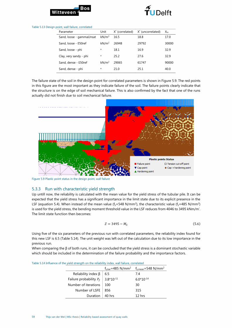
59 Thijs van der Wel | MSc thesis | Reliability based assessment of quay walls
Table 5.13 Design point, wall failure, correlated
Parameter Unit X* (correlated) X* (uncorrelated) Xm
Sand, loose - gammaUnsat kN/m3 16.5 18.8 17.0
Sand, loose - E50ref kN/m2 26948 29792 30000
Sand, loose - phi ᵒ 18.1 16.9 32.9
Clay, very sandy - phi ᵒ 25.2 27.6 32.9
Sand, dense - E50ref kN/m2 29065 61747 90000
Sand, dense - phi ᵒ 21.0 25.1 40.0
The failure state of the soil in the design point for correlated parameters is shown in Figure 5.9. The red points
in this figure are the most important as they indicate failure of the soil. The failure points clearly indicate that
the structure is on the edge of soil mechanical failure. This is also confirmed by the fact that one of the runs
actually did not finish due to soil mechanical failure.
Figure 5.9 Plastic point status in the design point, wall failure
5.3.3 Run with characteristic yield strength
Up untill now, the reliability is calculated with the mean value for the yield stress of the tubular pile. It can be
expected that the yield stress has a significant importance in the limit state due to its explicit presence in the
LSF (equation 5.4). When instead of the mean value (fy=548 N/mm2), the characteristic value (fy=485 N/mm2)
is used for the yield stress, the bending moment threshold value in the LSF reduces from 4046 to 3495 kNm/m’.
The limit state function then becomes:
𝑍 = 3495 −𝑀𝑆 (5.6)
Using five of the six parameters of the previous run with correlated parameters, the reliability index found for
this new LSF is 6.5 (Table 5.14). The unit weight was left out of the calculation due to its low importance in the
previous run.
When comparing the β of both runs, it can be concluded that the yield stress is a dominant stochastic variable
which should be included in the determination of the failure probability and the importance factors.
Table 5.14 Influence of the yield strength on the reliability index, wall failure, correlated
fy,kar=485 N/mm2 fy,mean=548 N/mm2
Reliability index β 6.5 7.4
Failure probability 𝑃𝑓 3.8*10-11 6.0*10-14
Number of iterations 100 30
Number of LSFE 856 315
Duration 40 hrs 12 hrs
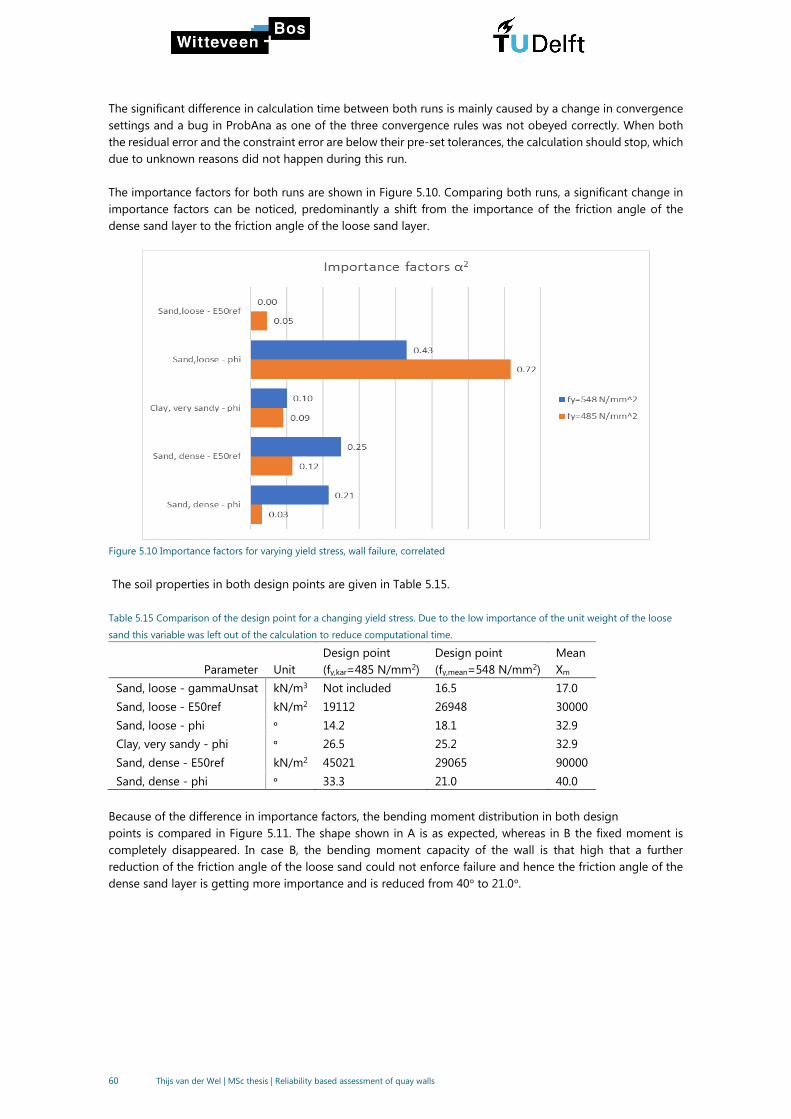
60 Thijs van der Wel | MSc thesis | Reliability based assessment of quay walls
The significant difference in calculation time between both runs is mainly caused by a change in convergence
settings and a bug in ProbAna as one of the three convergence rules was not obeyed correctly. When both
the residual error and the constraint error are below their pre-set tolerances, the calculation should stop, which
due to unknown reasons did not happen during this run.
The importance factors for both runs are shown in Figure 5.10. Comparing both runs, a significant change in
importance factors can be noticed, predominantly a shift from the importance of the friction angle of the
dense sand layer to the friction angle of the loose sand layer.
Figure 5.10 Importance factors for varying yield stress, wall failure, correlated
The soil properties in both design points are given in Table 5.15.
Table 5.15 Comparison of the design point for a changing yield stress. Due to the low importance of the unit weight of the loose
sand this variable was left out of the calculation to reduce computational time.
Parameter
Unit
Design point
(fy,kar=485 N/mm2)
Design point
(fy,mean=548 N/mm2)
Mean
Xm
Sand, loose - gammaUnsat kN/m3 Not included 16.5 17.0
Sand, loose - E50ref kN/m2 19112 26948 30000
Sand, loose - phi ᵒ 14.2 18.1 32.9
Clay, very sandy - phi ᵒ 26.5 25.2 32.9
Sand, dense - E50ref kN/m2 45021 29065 90000
Sand, dense - phi ᵒ 33.3 21.0 40.0
Because of the difference in importance factors, the bending moment distribution in both design
points is compared in Figure 5.11. The shape shown in A is as expected, whereas in B the fixed moment is
completely disappeared. In case B, the bending moment capacity of the wall is that high that a further
reduction of the friction angle of the loose sand could not enforce failure and hence the friction angle of the
dense sand layer is getting more importance and is reduced from 40° to 21.0°.
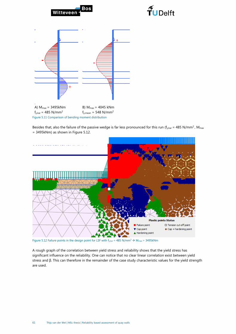
61 Thijs van der Wel | MSc thesis | Reliability based assessment of quay walls
A) Mmax = 3495kNm
fy,kar = 485 N/mm2
B) Mmax = 4045 kNm
fy,mean = 548 N/mm2
Figure 5.11 Comparison of bending moment distribution
Besides that, also the failure of the passive wedge is far less pronounced for this run (fy,kar = 485 N/mm2 , Mmax
= 3495kNm) as shown in Figure 5.12.
Figure 5.12 Failure points in the design point for LSF with fy,kar = 485 N/mm2
→ Mmax = 3495kNm
A rough graph of the correlation between yield stress and reliability shows that the yield stress has
significant influence on the reliability. One can notice that no clear linear correlation exist between yield
stress and β. This can therefore in the remainder of the case study characteristic values for the yield strength
are used.

62 Thijs van der Wel | MSc thesis | Reliability based assessment of quay walls
Figure 5.13 Yield stress vs. reliability
5.3.4 Influence of time-dependent loads
Until now only the soil is taken as random variable together with a deterministic normative load combination.
To determine the influence of the water level difference and the surcharge load, a run is performed assuming
both variables as stochastic.
The following distribution are assumed for the water level and the load:
Table 5.16 Distributions for the outer water level and the surcharge load
Distribution Mean Standard deviation
OWL Normal -0.84 m 0.20 m
Surcharge load Normal 40 kPa 8 kPa
To keep the number of variables limited, only the outer water level is taken as a variable, leaving the ground
water level constant. Ground water level and outer water level have a relatively high correlation in case of a
functioning drainage. Therefore assuming only one of the two as stochastic will most likely not lead to very
different results than when assuming both as stochastic as long as this is taken into account in the standard
deviation of OWL.
The standard deviations in Table 5.16 are based on an educated guess. For the distribution of the OWL the
extreme water level distributions shown in Figure 5.14 were taken into consideration.

63 Thijs van der Wel | MSc thesis | Reliability based assessment of quay walls
Figure 5.14 PDF of the extreme value distributions of the OWL of the Maasvlakte
Table 5.17 Calculation results, wall failure, including time dependent load variables
Value
Reliability index β 5.5
Failure probability 𝑃𝑓 1.8*10-8
Parameter
Unit
Design point
(fy,kar=485 N/mm2)
Mean
Xm
Importance factor
α2
OWL m -1.11 -0.84 0.07
Surcharge load kPa -40.0 -40 0.00
Sand, moderate - gammaUnsat kN/m3 18.8 18.0 0.02
Sand, moderate - phi ᵒ 41.3 38.9 0.01
Sand, loose - gammaUnsat kN/m3 16.6 17.0 0.01
Sand, loose - E50ref kN/m2 29538 30000 0.00
Sand, loose - phi ᵒ 19.0 32.9 0.63
Clay, very sandy - phi ᵒ 27.5 32.9 0.10
Sand, dense - E50ref kN/m2 41124 90000 0.11
Sand, dense - phi ᵒ 35.3 40.0 0.05
Compared to the reliability index of the run with deterministic loads a slight decrease of 0.3 is obtained. A
remarkable result here is that the surcharge load has no influence at all, whereas the uncertainty in the water
level difference is not negligible. This comparison confirms the assumption that time dependent load variables
are only of minor importance with regard to the reliability.
5.3.5 Validation of Abdo-Rackwitz algorithm
The validity of the obtained results using the Abdo-Rackwitz algorithm, are checked by performing the exact
same run (wall failure with fy,kar = 485 N/mm2) with the COBYLA-algorithm. Ideally, the results should be
checked with a level III analysis like MC or DS, but this is outside of the possibilities due to their long calculation
time compared to FORM. The results of both FORM runs are given in Table 5.18, Table 5.19 and Figure 5.15.
No significant difference in reliability index can be noticed, while also the difference in design point is marginal
except for the stiffness of the loose sand.
The calculation time with COBYLA is much shorter. This can be partly linked to the fact that COBYLA does not
calculate gradients explicitly. Though the fact that the Abdo-Rackwitz calculation did not stop when both the
residual and the constraint error were below their maximum tolerance is the most importance cause for this
difference.
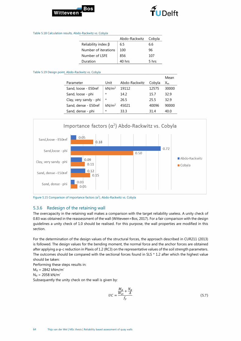
64 Thijs van der Wel | MSc thesis | Reliability based assessment of quay walls
Table 5.18 Calculation results, Abdo-Rackwitz vs. Cobyla
Abdo-Rackwitz Cobyla
Reliability index β 6.5 6.6
Number of iterations 100 96
Number of LSFE 856 107
Duration 40 hrs 5 hrs
Table 5.19 Design point, Abdo-Rackwitz vs. Cobyla
Parameter
Unit
Abdo-Rackwitz
Cobyla
Mean
Xm
Sand, loose - E50ref kN/m2 19112 12575 30000
Sand, loose - phi ᵒ 14.2 15.7 32.9
Clay, very sandy - phi ᵒ 26.5 25.5 32.9
Sand, dense - E50ref kN/m2 45021 40096 90000
Sand, dense - phi ᵒ 33.3 31.4 40.0
Figure 5.15 Comparison of importance factors (α2), Abdo-Rackwitz vs. Cobyla
5.3.6 Redesign of the retaining wall
The overcapacity in the retaining wall makes a comparison with the target reliability useless. A unity check of
0.83 was obtained in the reassessment of the wall (Witteveen+Bos, 2017). For a fair comparison with the design
guidelines a unity check of 1.0 should be realised. For this purpose, the wall properties are modified in this
section.
For the determination of the design values of the structural forces, the approach described in CUR211 (2013)
is followed. The design values for the bending moment, the normal force and the anchor forces are obtained
after applying a φ-c reduction in Plaxis of 1.2 (RC3) on the representative values of the soil strength parameters.
The outcomes should be compared with the sectional forces found in SLS * 1.2 after which the highest value
should be taken:
Performing these steps results in:
Md = 2842 kNm/m’
Nd = 2058 kN/m’
Subsequently the unity check on the wall is given by:
𝑈𝐶 =
𝑀𝑑𝑊𝑒𝑙
+𝑁𝑑𝐴
𝑓𝑦(5.7)
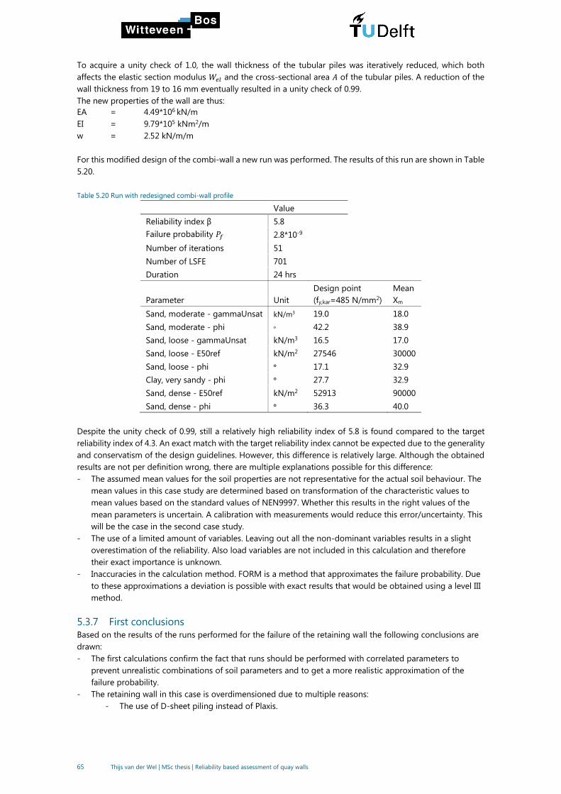
65 Thijs van der Wel | MSc thesis | Reliability based assessment of quay walls
To acquire a unity check of 1.0, the wall thickness of the tubular piles was iteratively reduced, which both
affects the elastic section modulus 𝑊𝑒𝑙 and the cross-sectional area 𝐴 of the tubular piles. A reduction of the
wall thickness from 19 to 16 mm eventually resulted in a unity check of 0.99.
The new properties of the wall are thus:
EA = 4.49*106 kN/m
EI = 9.79*105 kNm2/m
w = 2.52 kN/m/m
For this modified design of the combi-wall a new run was performed. The results of this run are shown in Table
5.20.
Table 5.20 Run with redesigned combi-wall profile
Value
Reliability index β 5.8
Failure probability 𝑃𝑓 2.8*10-9
Number of iterations 51
Number of LSFE 701
Duration 24 hrs
Parameter
Unit
Design point
(fy,kar=485 N/mm2)
Mean
Xm
Sand, moderate - gammaUnsat kN/m3 19.0 18.0
Sand, moderate - phi ᵒ 42.2 38.9
Sand, loose - gammaUnsat kN/m3 16.5 17.0
Sand, loose - E50ref kN/m2 27546 30000
Sand, loose - phi ᵒ 17.1 32.9
Clay, very sandy - phi ᵒ 27.7 32.9
Sand, dense - E50ref kN/m2 52913 90000
Sand, dense - phi ᵒ 36.3 40.0
Despite the unity check of 0.99, still a relatively high reliability index of 5.8 is found compared to the target
reliability index of 4.3. An exact match with the target reliability index cannot be expected due to the generality
and conservatism of the design guidelines. However, this difference is relatively large. Although the obtained
results are not per definition wrong, there are multiple explanations possible for this difference:
- The assumed mean values for the soil properties are not representative for the actual soil behaviour. The
mean values in this case study are determined based on transformation of the characteristic values to
mean values based on the standard values of NEN9997. Whether this results in the right values of the
mean parameters is uncertain. A calibration with measurements would reduce this error/uncertainty. This
will be the case in the second case study.
- The use of a limited amount of variables. Leaving out all the non-dominant variables results in a slight
overestimation of the reliability. Also load variables are not included in this calculation and therefore
their exact importance is unknown.
- Inaccuracies in the calculation method. FORM is a method that approximates the failure probability. Due
to these approximations a deviation is possible with exact results that would be obtained using a level III
method.
5.3.7 First conclusions
Based on the results of the runs performed for the failure of the retaining wall the following conclusions are
drawn:
- The first calculations confirm the fact that runs should be performed with correlated parameters to
prevent unrealistic combinations of soil parameters and to get a more realistic approximation of the
failure probability.
- The retaining wall in this case is overdimensioned due to multiple reasons:
- The use of D-sheet piling instead of Plaxis.

66 Thijs van der Wel | MSc thesis | Reliability based assessment of quay walls
- The choice for a thicker profile due to practical and financial reasons (during construction, thicker
tubular piles were better available and for a good price)
- The yield stress has significant influence on the limit state and therefore either a conservative value
should be chosen or preferably it should be selected as stochastic variable and directly implemented in
FORM.
- As already expected the computational times are long, usually in the order of a day.
- The results of COBYLA and Abdo-Rackwitz are comparable in this case. Therefore COBYLA might be
useful when only a few random variables are of interest.
- The uncertainty in time dependent load variables have only minor contribution to the reliability index of
the retaining wall
5.4 LS2: Yielding of the anchor rod
In this section the exceedance of yield stress in the anchor rod is considered. First, the reliability of the anchor
is determined for the original design because in the reassessment it appeared that this element of the quay
wall was critical due to the unity check of 1.12 (Witteveen+Bos, 2017).
The LSF for this failure criterion was given by:
𝑍 = 𝑓𝑦𝐴𝑎𝑛𝑐ℎ𝑜𝑟 − 𝑁𝑆 (5.8)
Since the tubular piles are double anchored and both anchors have deviating structural properties, also two
limit state functions can be formulated. However, during previous calculations it already became clear that the
upper anchor is always the most critical one and therefore only this anchor is assessed.
Since a deterministic value for the yields stress 𝑓𝑦 should be chosen, and given the significant importance of
the yield stress in previous research (Teixeira et al. (2015), Wolters (2012)) the characteristic value is used here
instead of the mean value. Also a deterministic value for 𝐴𝑎𝑛𝑐ℎ𝑜𝑟 is assumed. Firstly, the reliability is calculated
for an uncorroded cross-section:
𝑓𝑦𝐴𝑎𝑛𝑐ℎ𝑜𝑟 = 500𝑁 𝑚𝑚2⁄ ∗ 5510𝑚𝑚2 = 2755𝑘𝑁
Filling this into the LSF:
𝑍 = 2755 − 𝑁𝑆 (5.9)
For the sensitivity analysis, again uncorrelated variables are used to determine the most important parameters.
Besides 𝛾𝑢𝑛𝑠𝑎𝑡 , 𝜑′ and 𝐸50𝑟𝑒𝑓
, also the interface strength 𝑅𝑖𝑛𝑡𝑒𝑟 is taken as stochastic. Given the fact that the soil
adjacent to the retaining wall settles more than the wall itself, a smaller interface strength causes a smaller
vertical load on the wall, which reduces the vertical downward force on the anchor rod resulting in a larger
tension force.
The interface strength depends for a large part on the friction angle, therefore the same COV as for the friction
angle is applied. A truncated normal distribution is used to prevent that values smaller than 0.0 or larger than
1.0 are used. The results of the sensitivity analysis are shown in Figure 5.16.

67 Thijs van der Wel | MSc thesis | Reliability based assessment of quay walls
Figure 5.16 Importance factors sensitivity analysis anchor, uncorrelated
It can be noticed that this problem is mainly dominated by the friction angle and the unit soil weight, whereas
the stiffness and the interface strength in total only have an influence of 1%. The friction angle of the loose
sand layer is dominating this problem, as this was also the case for the retaining wall.
Based on this results the failure probability is determined with only 8 (correlated) parameters.
Figure 5.17 Importance factors anchor, correlated
The reliability index determined with this run is 7.6. When checking the results, it is remarkable that the
saturated unit weight and the stiffness of the loose sand barely decrease, whereas the friction angle of this
layer is heavily reduced. Due to the use of correlations one might expect that these two parameters are also
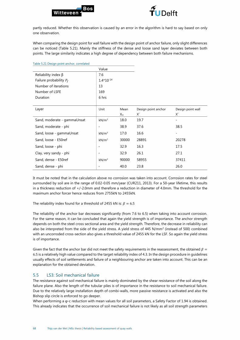
68 Thijs van der Wel | MSc thesis | Reliability based assessment of quay walls
partly reduced. Whether this observation is caused by an error in the algorithm is hard to say based on only
one observation.
When comparing the design point for wall failure with the design point of anchor failure, only slight differences
can be noticed (Table 5.21). Mainly the stiffness of the dense and loose sand layer deviates between both
points. The large similarity indicates a high degree of dependency between both failure mechanisms.
Table 5.21 Design point anchor, correlated
Value
Reliability index β 7.6
Failure probability 𝑃𝑓 1.4*10-14
Number of iterations 13
Number of LSFE 169
Duration 6 hrs
Layer Unit Mean
Xm
Design point anchor
X*
Design point wall
X*
Sand, moderate - gammaUnsat kN/m3 18.0 19.7 -
Sand, moderate - phi ᵒ 38.9 37.6 38.5
Sand, loose - gammaUnsat kN/m3 17.0 16.6 -
Sand, loose - E50ref kN/m2 30000 28891 20278
Sand, loose - phi ᵒ 32.9 16.3 17.5
Clay, very sandy - phi ᵒ 32.9 26.1 27.1
Sand, dense - E50ref kN/m2 90000 58955 37411
Sand, dense - phi ᵒ 40.0 23.8 26.0
It must be noted that in the calculation above no corrosion was taken into account. Corrosion rates for steel
surrounded by soil are in the range of 0.02-0.05 mm/year (CUR211, 2013). For a 50-year lifetime, this results
in a thickness reduction of +/-2.0mm and therefore a reduction in diameter of 4.0mm. The threshold for the
maximum anchor forcer hence reduces from 2755kN to 2455kN.
The reliability index found for a threshold of 2455 kN is: 𝛽 = 6.5
The reliability of the anchor bar decreases significantly (from 7.6 to 6.5) when taking into account corrosion.
For the same reason, it can be concluded that again the yield strength is of importance. The anchor strength
depends on both the steel cross sectional area and the yield strength. Therefore, the decrease in reliability can
also be interpreted from the side of the yield stress. A yield stress of 445 N/mm2 (instead of 500) combined
with an uncorroded cross-section also gives a threshold value of 2455 kN for the LSF. So again the yield stress
is of importance.
Given the fact that the anchor bar did not meet the safety requirements in the reassessment, the obtained 𝛽 =
6.5 is a relatively high value compared to the target reliability index of 4.3. In the design procedure in guidelines
usually effects of soil settlements and failure of a neighbouring anchor are taken into account. This can be an
explanation for the obtained deviation.
5.5 LS3: Soil mechanical failure
The resistance against soil mechanical failure is mainly dominated by the shear resistance of the soil along the
failure plane. Also the length of the tubular piles is of importance in the resistance to soil mechanical failure.
Due to the relatively large installation depth of combi-walls, more passive resistance is activated and also the
Bishop slip circle is enforced to go deeper.
When performing a φ-c reduction with mean values for all soil parameters, a Safety Factor of 1.94 is obtained.
This already indicates that the occurrence of soil mechanical failure is not likely as all soil strength parameters
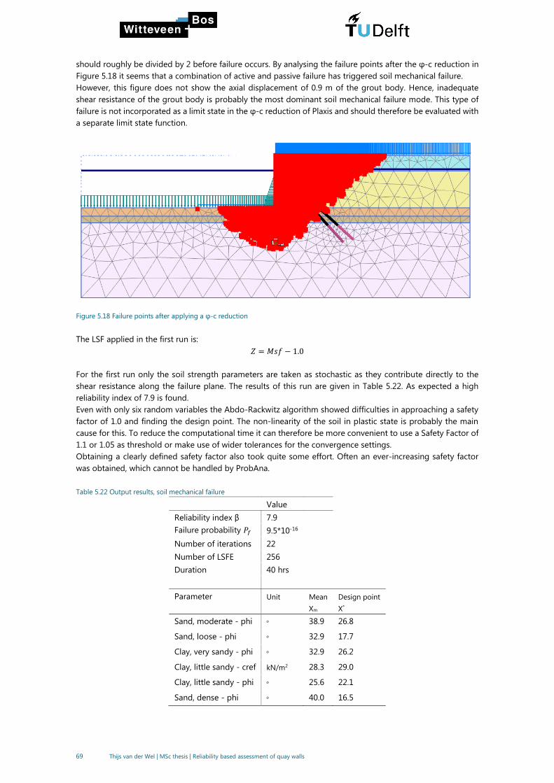
69 Thijs van der Wel | MSc thesis | Reliability based assessment of quay walls
should roughly be divided by 2 before failure occurs. By analysing the failure points after the φ-c reduction in
Figure 5.18 it seems that a combination of active and passive failure has triggered soil mechanical failure.
However, this figure does not show the axial displacement of 0.9 m of the grout body. Hence, inadequate
shear resistance of the grout body is probably the most dominant soil mechanical failure mode. This type of
failure is not incorporated as a limit state in the φ-c reduction of Plaxis and should therefore be evaluated with
a separate limit state function.
Figure 5.18 Failure points after applying a φ-c reduction
The LSF applied in the first run is:
𝑍 = 𝑀𝑠𝑓 − 1.0
For the first run only the soil strength parameters are taken as stochastic as they contribute directly to the
shear resistance along the failure plane. The results of this run are given in Table 5.22. As expected a high
reliability index of 7.9 is found.
Even with only six random variables the Abdo-Rackwitz algorithm showed difficulties in approaching a safety
factor of 1.0 and finding the design point. The non-linearity of the soil in plastic state is probably the main
cause for this. To reduce the computational time it can therefore be more convenient to use a Safety Factor of
1.1 or 1.05 as threshold or make use of wider tolerances for the convergence settings.
Obtaining a clearly defined safety factor also took quite some effort. Often an ever-increasing safety factor
was obtained, which cannot be handled by ProbAna.
Table 5.22 Output results, soil mechanical failure
Value
Reliability index β 7.9
Failure probability 𝑃𝑓 9.5*10-16
Number of iterations 22
Number of LSFE 256
Duration 40 hrs
Parameter Unit Mean
Xm
Design point
X*
Sand, moderate - phi ᵒ 38.9 26.8
Sand, loose - phi ᵒ 32.9 17.7
Clay, very sandy - phi ᵒ 32.9 26.2
Clay, little sandy - cref kN/m2 28.3 29.0
Clay, little sandy - phi ᵒ 25.6 22.1
Sand, dense - phi ᵒ 40.0 16.5
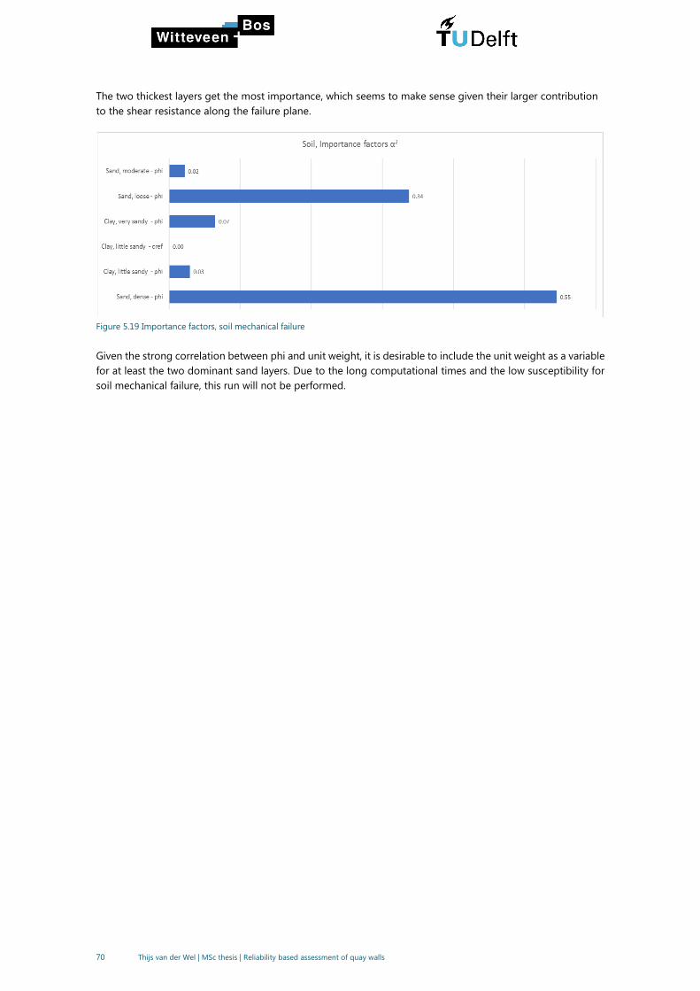
70 Thijs van der Wel | MSc thesis | Reliability based assessment of quay walls
The two thickest layers get the most importance, which seems to make sense given their larger contribution
to the shear resistance along the failure plane.
Figure 5.19 Importance factors, soil mechanical failure
Given the strong correlation between phi and unit weight, it is desirable to include the unit weight as a variable
for at least the two dominant sand layers. Due to the long computational times and the low susceptibility for
soil mechanical failure, this run will not be performed.

71 Thijs van der Wel | MSc thesis | Reliability based assessment of quay walls
5.6 Intermediate conclusion
After the three considered failure mechanisms have been assessed, some first conclusions can be drawn.
The conclusion has been subdivided into a part about the reliability of the considered structure and a part
about the functioning of the Plaxis-FORM coupling.
5.6.1 Reliability of the structure
Regarding the limit states yielding of the wall, yielding of the anchor profile and soil mechanical failure, the
structure can be considered very safe. Whether the overall reliability of the structure is sufficient cannot be
concluded as not all failure mechanisms are checked. Especially the failure mechanism ‘Shear resistance of the
grout body inadequate’ should be checked as this was a critical failure mode in the reassessment of this quay
wall (Witteveen+Bos, 2017).
Table 5.23 Obtained reliability indices for the as-built LBBR quay wall
Limit state Reliability index β
Yielding of the retaining wall 6.5
Yielding of the anchor steel profile 6.5
Soil mechanical failure 7.9
For the failure mechanism yielding of the combi-wall, a clear comparison with the design guidelines was
performed by reducing the wall thickness compared to the ass-built wall thickness to acquire a unity check of
0.99. Subsequently, the obtained reliability index when including both soil and variable loads as stochastic was:
𝛽𝑦𝑖𝑒𝑙𝑑𝑖𝑛𝑔,𝑤𝑎𝑙𝑙 = 5.5
This confirms the expectation that a semi-probabilistic design generally results in a higher reliability index than
required by design codes. However, more structures should be assessed to be able to give a more sound
conclusion about this assumption.
For the LBBR quay wall, the uncertainty in the soil parameters is the most dominant uncertainty of which
furthermore the friction angle is the most dominant soil property. The uncertainty in the friction angle is
reducible by performing measurements and apply this in a Bayesian update. In this way an increase in reliability
can be obtained, making way for a possible load increase.
The strong correlation between yield stress and reliability for both the anchor and wall yielding implies that
also the yield stress is a dominant uncertainty.
The influence of uncertainty in variable loads seems only minor for the limit state yielding of the wall. Whether
this also holds for other failure mechanisms should be investigated.
5.6.2 Plaxis-FORM coupling (ProbAna)
The goal of this case study was also to gather experience with probabilistic calculations and to test the
applicability of FORM for the three considered limit states. In general it can be concluded that for failure of
the structural elements, FORM performed reasonably well. Whether convergence is reached highly depends
on the maximum convergence errors. For convergence of structural elements the following errors are
dominant:
· Absolute error
· Residual error
At first a maximum error of 1% was used. However, this resulted several times in non-convergence. Therefore
the maximum error was increased to 5%. With this value convergence was reached most of the time, whereas
it is still considered a reasonable tolerance to obtain accurate results.
Other problems that were encountered are:
· Plasticity in the initial phase
· Problems with the input restrictions of Plaxis for 𝐸𝑜𝑒𝑑 and 𝐾0𝑛𝑐
72 Thijs van der Wel | MSc thesis | Reliability based assessment of quay walls
The first problem was only encountered when using the K0-procedure in Plaxis to determine the initial stresses
in the soil and was caused by a bug in ProbAna. To tackle this, gravity loading was used instead.
Regarding the second bullet, this is not a flaw of ProbAna, but more a consequence of the use of probabilistic
methods in combination with Plaxis. When Plaxis does not accept the input values determined by the FORM
algorithm, the calculation is stopped and no results are available. The calculation should be started all over
again from the start.
To limit the occurrence of this error, the ratio between E50 and Eoed, was slightly adapted from 1 : 1 to
approximately 1 : 0.8 whereas also very high mean values of E50 were reduced to 80 MPa. As the importance
of the stiffness was in general not very large, these adjustments are assumed to not influence the reliability
index by much.
With these adjustments, results were obtained in most cases.
Regarding soil mechanical failure, at first difficulties were encountered in reaching a clearly defined safety
factor using the phi-c reduction method. Thereafter the convergence to a safety factor of 1.0 took considerably
more iterations compared to a limit state for a structural element. This is also caused due to the fact that the
starting point (Msf = 1.94) was far away from the threshold (1.0) and a different approach in the line-search
algorithm of AR compared to other limit states. Unfortunately, the starting point cannot be adjusted with the
current package.
Also the Cobyla algorithm was tested for this failure mechanism. This algorithm converged two times to a
wrong design point (a Msf of 1.4) and was therefore not used further throughout this thesis.
In general, with the Abdo-Rackwitz algorithm convergence can be reached, although taking quite some effort
and computation time.
Change in software package
At this point, it was decided to upgrade the version of ProbAna to a more advanced custom version of ProbAna,
from now on referred to as ProbAna2018, as the version used up till now is from 2017. The main
reason/advantages of this upgrade are:
· Intermediate results are saved and available in case of an unfinished calculation.
· The algorithm can start at a starting point given by the user instead of the standard starting point
(median values). This allows to continue a calculation after an error has occurred or when Plaxis has
frozen or when previous knowledge about the design point is available.
· Properties of structural elements can be considered as stochastic.
· More freedom in the definition of the limit state function and more choice in distribution types.
The first two advantages save a lot of calculation time, whereas the last two can increase the validity of the
results. All calculations in the remainder of this thesis are performed with the upgraded toolkit.
Additional calculations
After the change in toolkit and the experience gathered with performing probabilistic calculations, additional
calculations are performed for this quay wall to achieve the following two objectives:
1 Determine the reliability index for the limit state: shear resistance of anchorage inadequate
2 Deriving a set of partial factors
These objectives are treated in the next two paragraphs.
73 Thijs van der Wel | MSc thesis | Reliability based assessment of quay walls
5.7 LS4: Shear resistance of anchorage inadequate
The assessment of the reliability regarding soil mechanical failure showed that slipping of the grout body is
the most dominant soil failure mode. However, in that calculation the shear resistance of the grout body itself
is not considered stochastic, whereas there is quite some uncertainty in the resistance of a grout body and the
modelling in Plaxis. With ProbAna2018, the strength of the grout body can be assessed individually, which is
treated in this chapter.
In general, the strength of a grout body is calculated with:
𝐹𝑟𝑒𝑠,𝑔𝑟𝑜𝑢𝑡 = 𝛼𝑡 ∗ 𝑞𝑐 ∗ 𝐿 ∗ 𝑂 (5.11)
In which
𝐹𝑟𝑒𝑠,𝑔𝑟𝑜𝑢𝑡 Resistance of the grout body [kN]
𝛼𝑡 Pile class factor [-]
𝑞𝑐 Cone resistance [MPa]
𝐿 Length of the grout body [m]
𝑂 Circumference of the grout body [m] (𝑂 = 𝜋 ∗ 𝐷)
This results in the following LSF:
𝑍 = 𝛼𝑡 ∗ 𝑞𝑐 ∗ 𝐿 ∗ 𝑂 − 𝑁𝑆 (5.12)
In which 𝑁𝑆 is the normal force in the steel anchor bar.
The empirical value 𝛼𝑡 describes the ratio between the cone resistance at the location of the grout body and
the shear resistance 𝜏 along the grout body and is derived by:
𝛼𝑡 =𝜏
𝑞𝑐(5.13)
For self-boring grout injection piles in sand, the design value of 𝛼𝑡 ranges from 0.008 as lower bound in case
no in-situ tests are performed, up to a value of 0.012 when in-situ tests are performed (CUR236, 2011). Two
important notes regarding these values are:
1 The cone resistance should be cut of at 20 MPa ( in Dutch: afsnuiten), which implies that when a higher
cone resistance than 20 MPa is measured at the location of the grout body, still 20 MPa should be used
in equation 5.11.
2 The value of 0.012 is a design value, the expected value is generally higher.
These two remarks will become more clear when looking at the results of several in-situ test loadings shown
in Figure 5.20. The dashed line in this figure illustrates the safe design value of 𝛼𝑡 = 0.012. All test loading
results are above this line. The solid line represents 𝛼𝑡 = 0.015, which seems to represent the expected value
quite well, especially for a cone resistance up to 20 MPa.
The results of the test loading at the location of LBBR are shown as green dots in Figure 5.20. Although the
results indicate a good fit with an 𝛼𝑡 = 0.015, it must be noted that the grout body is not tested up till failure
because the yield strength of the steel bar was limiting a further load increase. Taking this into consideration
together with the test results for a cone resistance of 34 MPa, one might argue the validity of a complete cut-
off at 20 MPa. In these cases with high cone resistance, a value of 𝛼𝑡 = 0.015 seems conservative. However,
too few test results are available here to give a sound argumentation for this presumption.
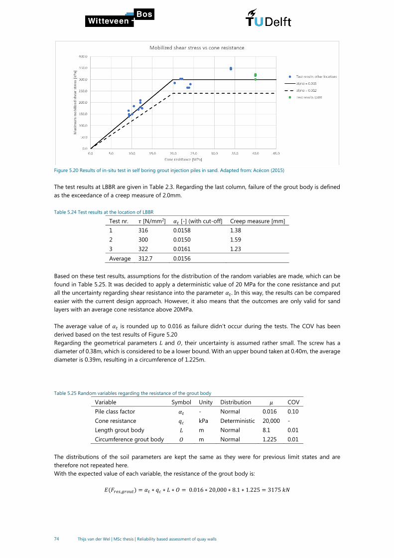
74 Thijs van der Wel | MSc thesis | Reliability based assessment of quay walls
Figure 5.20 Results of in-situ test in self boring grout injection piles in sand. Adapted from: Acécon (2015)
The test results at LBBR are given in Table 2.3. Regarding the last column, failure of the grout body is defined
as the exceedance of a creep measure of 2.0mm.
Table 5.24 Test results at the location of LBBR
Test nr. 𝜏 [N/mm2] 𝛼𝑡 [-] (with cut-off] Creep measure [mm]
1 316 0.0158 1.38
2 300 0.0150 1.59
3 322 0.0161 1.23
Average 312.7 0.0156
Based on these test results, assumptions for the distribution of the random variables are made, which can be
found in Table 5.25. It was decided to apply a deterministic value of 20 MPa for the cone resistance and put
all the uncertainty regarding shear resistance into the parameter 𝛼𝑡. In this way, the results can be compared
easier with the current design approach. However, it also means that the outcomes are only valid for sand
layers with an average cone resistance above 20MPa.
The average value of 𝛼𝑡 is rounded up to 0.016 as failure didn’t occur during the tests. The COV has been
derived based on the test results of Figure 5.20
Regarding the geometrical parameters 𝐿 and 𝑂, their uncertainty is assumed rather small. The screw has a
diameter of 0.38m, which is considered to be a lower bound. With an upper bound taken at 0.40m, the average
diameter is 0.39m, resulting in a circumference of 1.225m.
Table 5.25 Random variables regarding the resistance of the grout body
Variable Symbol Unity Distribution 𝜇 COV
Pile class factor 𝛼𝑡 - Normal 0.016 0.10
Cone resistance 𝑞𝑐 kPa Deterministic 20,000 -
Length grout body 𝐿 m Normal 8.1 0.01
Circumference grout body 𝑂 m Normal 1.225 0.01
The distributions of the soil parameters are kept the same as they were for previous limit states and are
therefore not repeated here.
With the expected value of each variable, the resistance of the grout body is:
𝐸(𝐹𝑟𝑒𝑠,𝑔𝑟𝑜𝑢𝑡) = 𝛼𝑡 ∗ 𝑞𝑐 ∗ 𝐿 ∗ 𝑂 = 0.016 ∗ 20,000 ∗ 8.1 ∗ 1.225 = 3175𝑘𝑁

75 Thijs van der Wel | MSc thesis | Reliability based assessment of quay walls
Which is higher than the expected yield limit of the steel anchor rod: 2774 kN.
Results
The results of the calculation for this limit state are given in Table 5.26 and Figure 5.21. The calculated reliability
index for this limit state is 4.9, which is considerably lower than the value found for soil mechanical failure (4.9
vs 7.9). The main reason for this deviation is the large difference in limit state functions.
As Figure 5.21 shows, the problem is mainly dominated by the uncertainty in the parameter 𝛼𝑡, which has a
value of 0.009 in the design point.
It is therefore worthwhile to consider the validity of the assumed distribution of 𝛼𝑡.

76 Thijs van der Wel | MSc thesis | Reliability based assessment of quay walls
Table 5.26 Calculation information for limit state 4
Value
Reliability index β 4.9
Failure probability 𝑃𝑓 5.0*10-7
Number of iterations 1
Number of LSFE 20
Duration 0.4 hrs
Parameter
Unit
Design point
X*
Mean
Xm
Sand, moderate - φ’ ᵒ 38.25 38.9
Sand, loose - φ’ ᵒ 26.89 32.9
Clay, very sandy - φ’ ᵒ 30.77 32.9
Sand, dense - φ’ ᵒ 38.93 40.0
Sand, moderate - E50ref kN/m2 48715 45000
Sand, loose - E50ref kN/m2 26925 30000
Clay, very sandy - E50ref kN/m2 14521 16000
Sand, dense - E50ref kN/m2 70369 70000
Sand, moderate - γunsat kN/m3 18.46 18.0
Sand, loose - γunsat kN/m3 16.59 17.0
Clay, very sandy - γunsat kN/m3 17.53 18.0
Sand, dense - γunsat kN/m3 18.89 19.0
𝛼𝑡 - 0.009 0.016
L m 8.056 8.1
qc kPa 20000 20000
O m 1.222 1.225
Figure 5.21 Importance factors limit state grout body
The parameters of the distribution of 𝛼𝑡 are determined based on only a few test results that were all in the
range of 0.013-0.018. It is therefore questionable whether the chosen normal distribution is also valid for values
that lie far away from this range, such as the value of 0.009. Besides, in practice it is obliged to perform in-situ
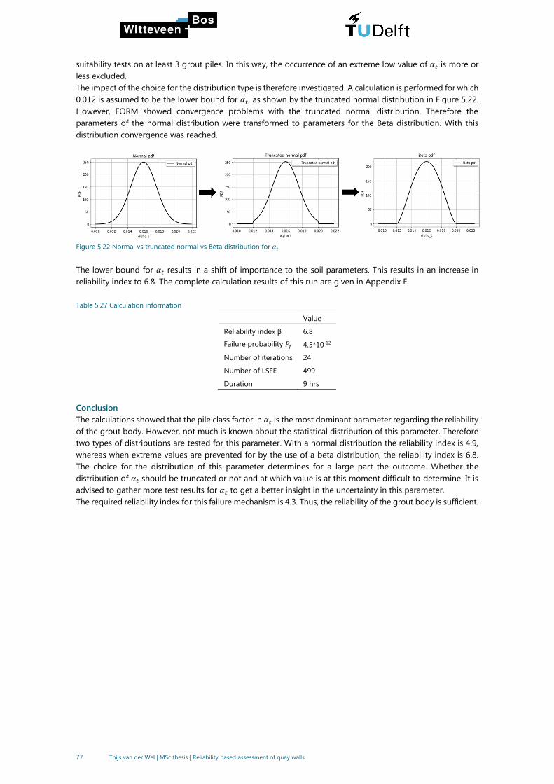
77 Thijs van der Wel | MSc thesis | Reliability based assessment of quay walls
suitability tests on at least 3 grout piles. In this way, the occurrence of an extreme low value of 𝛼𝑡 is more or
less excluded.
The impact of the choice for the distribution type is therefore investigated. A calculation is performed for which
0.012 is assumed to be the lower bound for 𝛼𝑡, as shown by the truncated normal distribution in Figure 5.22.
However, FORM showed convergence problems with the truncated normal distribution. Therefore the
parameters of the normal distribution were transformed to parameters for the Beta distribution. With this
distribution convergence was reached.
Figure 5.22 Normal vs truncated normal vs Beta distribution for 𝛼𝑡
The lower bound for 𝛼𝑡 results in a shift of importance to the soil parameters. This results in an increase in
reliability index to 6.8. The complete calculation results of this run are given in Appendix F.
Table 5.27 Calculation information
Value
Reliability index β 6.8
Failure probability 𝑃𝑓 4.5*10-12
Number of iterations 24
Number of LSFE 499
Duration 9 hrs
Conclusion
The calculations showed that the pile class factor in 𝛼𝑡 is the most dominant parameter regarding the reliability
of the grout body. However, not much is known about the statistical distribution of this parameter. Therefore
two types of distributions are tested for this parameter. With a normal distribution the reliability index is 4.9,
whereas when extreme values are prevented for by the use of a beta distribution, the reliability index is 6.8.
The choice for the distribution of this parameter determines for a large part the outcome. Whether the
distribution of 𝛼𝑡 should be truncated or not and at which value is at this moment difficult to determine. It is
advised to gather more test results for 𝛼𝑡 to get a better insight in the uncertainty in this parameter.
The required reliability index for this failure mechanism is 4.3. Thus, the reliability of the grout body is sufficient.

78 Thijs van der Wel | MSc thesis | Reliability based assessment of quay walls
5.8 Derivation of partial factors
The calculations in the previous paragraphs showed the overcapacity in the design even when the unity check
for a certain failure mechanism is larger than 1.0. This is for a large part caused by the conservatism in the
design codes regarding partial factors. The code takes into account modelling uncertainty and is developed in
such a way that roughly 95% of the designs has the same or a higher reliability index than required.
In this paragraph the partial factors are derived on this quay structure to be able to have a discussion about
the magnitude of the current partial factors.
5.8.1 Approach
For this purpose, the reliability index and sensitivity factors for the failure mechanisms yielding of the combi-
wall and yielding of the anchor bar are calculated again, The main reason for a recalculation is the fact that
structural properties formerly could not be included. Next to that, ProbAna2018 is better capable of handling
large amount of variables. Therefore more soil parameters could be included compared to the initial
calculations, which is preferable with respect to the correlations between soil parameters.
The calculations are performed using the adjusted design (see Chapter 5.3.6), because the original design has
too much overcapacity with respect to the failure mechanism ‘yielding of the wall’. This can result in an
inaccurate representation of the sensitivity factors. The only adjustment that was made, was a reduction in wall
thickness from 19mm to 16mm. For the failure mechanism soil mechanical failure no additional calculations
were performed as this would be too time-consuming.
The structure is designed for RC3, so the partial factors will also be derived for this class. The target reliability
at component level for this class is 4.3 .
For the derivation of the partial factors with the results of a FORM calculation ideally each partial factor is
derived by:
𝛾𝑖 =𝑋𝑘,𝑖𝑋𝑖∗ =
𝜇𝑖 − 𝑘𝜎𝑖
𝑋𝑖∗ (5.14)
In which
𝜇𝑖 Mean value of variable 𝑋𝑖
𝜎𝑖 Standard deviation of variable 𝑋𝑖
𝑋𝑘,𝑖 Characteristic value of parameter 𝑋𝑖
𝑋𝑖∗ Design value of parameter 𝑋𝑖 obtained from FORM
𝑘 factor representing the distance from the mean to the characteristic value in units of standard
deviation. (k = 1.645 for a 5% under exceedance value )
With this method the partial factors are derived for the reliability index 𝛽𝐹𝑂𝑅𝑀 that is obtained with the FORM
calculation. However, this reliability index is not always equal to the desired reliability index of the design code
(referred to 𝛽𝑅𝐶3 from now on). In this thesis, the obtained reliability indices are often higher than the required
reliability indices. Therefore, when applying equation 5.14 the partial factors would result in too high partial
factors. It would be time consuming to create a design that almost exactly approaches the required reliability
index such that: 𝛽𝐹𝑂𝑅𝑀 ≈ 𝛽𝑅𝐶3. This is also not per definition needed. To derive the design point for the
required 𝛽𝑅𝐶3, the following equations are used:
For normal distributions:
𝑋𝑖,𝑅𝐶3∗ = 𝜇𝑋𝑖 − 𝛼𝑖 𝛽𝑅𝐶3𝜎𝑋𝑖 (5.15)
For lognormal distributions:
𝑋𝑖,𝑅𝐶3∗ =
𝜇𝑋𝑖
√1+𝐶𝑂𝑉𝑖2exp (−𝛼𝑖 𝛽𝑅𝐶3√ln(1 + 𝐶𝑂𝑉𝑖
2)) (5.16)
The partial factor for a resistance parameter is then derived by:

79 Thijs van der Wel | MSc thesis | Reliability based assessment of quay walls
𝛾𝑅,𝑖 =𝑋𝑘,𝑖𝑋𝑖,𝑅𝐶3∗ =
𝜇𝑖 − 𝑘𝜎𝑖
𝜇𝑖 − 𝛼𝑖 𝛽𝑅𝐶3𝜎𝑖=
𝜇𝑖(1 − 𝑘𝑉𝑖)
𝜇𝑖(1 − 𝛼𝑖 𝛽𝑅𝐶3𝑉𝑖)=
1 − 𝑘𝑉𝑖1 − 𝛼𝑖 𝛽𝑅𝐶3𝑉𝑖
(5.17)
In which
𝛼𝑖 Sensitivity factor of random variable 𝑋𝑖 obtained from a FORM calculation
𝛽𝑅𝐶3 Required reliability index for RC3
𝑋𝑖,𝑅𝐶3∗ Design value corresponding to 𝛽𝑅𝐶3
𝑉𝑖 Coefficient of variation of random variable 𝑋𝑖
𝑘 factor representing the distance from the mean to the characteristic value in units of standard
deviation. (k = 1.645 for a 5% under exceedance value)
The most important assumption with this method is that the sensitivity factors (𝛼𝑖) do not significantly change
for a slightly different reliability index. It is assumed that this is the case for this quay wall. The obtained
reliability indices are in general one point higher than the required reliability indices. It should be checked with
an additional calculation whether the assumption is valid.
OpenTURNS provides two types of sensitivity factors: Sensitivity factors in the U-space and sensitivity factors
in the Y-space. The sensitivity factors in the U-space are decorrelated, therefore the ordering of the variables
influences the magnitude of the sensitivity factors. For the importance factors in the Y-space, this problem
does not occur as these factors are derived from the design point in the physical space (X-space) and therefore
correlations are taken into account correctly. These factors should therefore be used to derive the partial
factors.
5.8.2 LS1: Yielding of the wall
The applied LSF for wall failure (yielding) is:
𝑍 = 𝑓𝑦 −max [|𝑀(𝑧)|
𝑊𝑒𝑙+|𝑁(𝑧)|
𝐴𝑤𝑎𝑙𝑙] (5.18)
The values of 𝐴𝑤𝑎𝑙𝑙 and 𝑊𝑒𝑙 are automatically calculated based on the input for the pile diameter 𝐷 and the
wall thickness 𝑡. The applied distributions 𝐷, 𝑡 and 𝑓𝑦 for are given in chapter 4.3. The characteristic values of
the unit weight, the wall thickness and the tube diameter are assumed to be equal to the mean values.
The results of the FORM run and the derivation of the partial factors are shown in Table 5.28. The partial factors
on 𝜑 given in this table should be applied on tan(𝜑𝑘). In this section, less attention will be given to the
geotechnical explanation of the obtained results as this was already described in detail for each failure mode
earlier on in this chapter. When a partial factor should be applied on a mean, the characteristic value is taken
equal to the mean value.
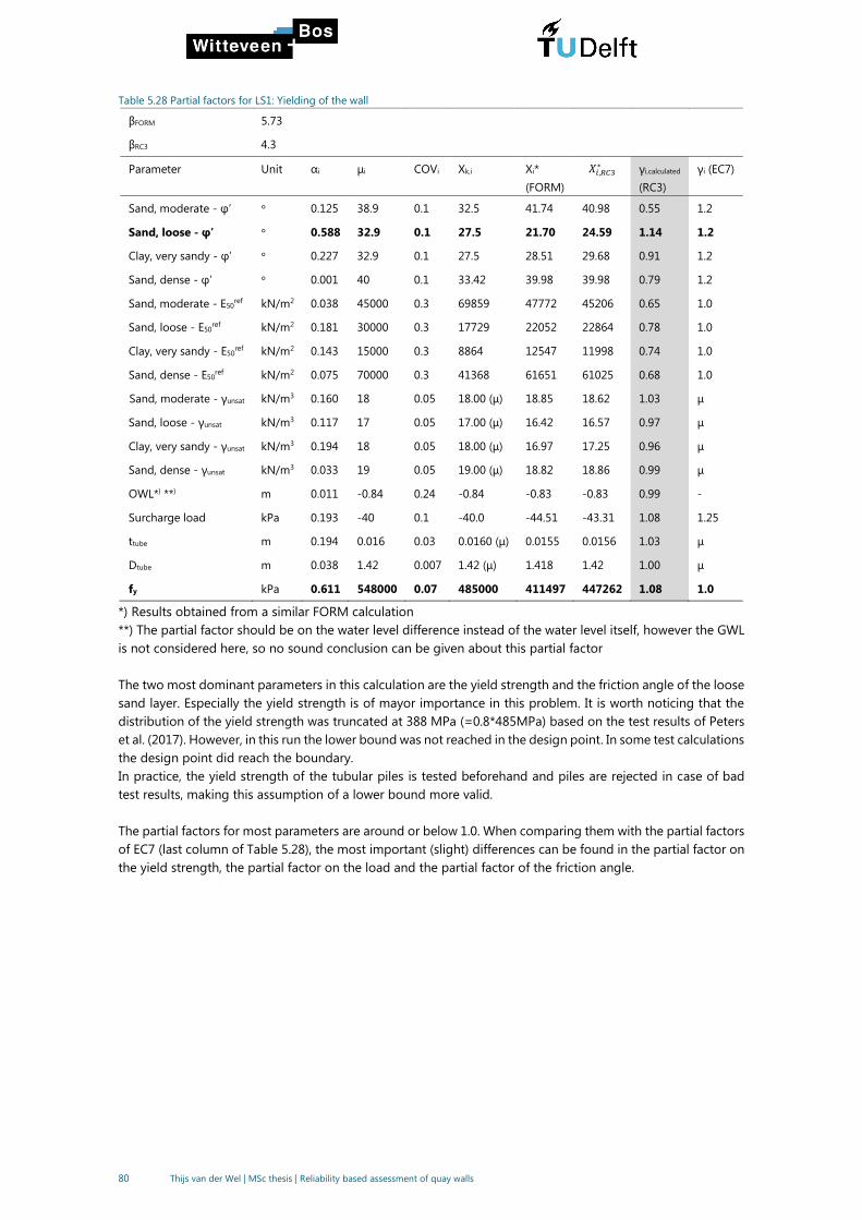
80 Thijs van der Wel | MSc thesis | Reliability based assessment of quay walls
Table 5.28 Partial factors for LS1: Yielding of the wall
βFORM 5.73
βRC3 4.3
Parameter Unit αi μi COVi Xk,i Xi*
(FORM)
𝑋𝑖,𝑅𝐶3∗ γi,calculated
(RC3)
γi (EC7)
Sand, moderate - φ’ ° 0.125 38.9 0.1 32.5 41.74 40.98 0.55 1.2
Sand, loose - φ’ ° 0.588 32.9 0.1 27.5 21.70 24.59 1.14 1.2
Clay, very sandy - φ’ ° 0.227 32.9 0.1 27.5 28.51 29.68 0.91 1.2
Sand, dense - φ’ ° 0.001 40 0.1 33.42 39.98 39.98 0.79 1.2
Sand, moderate - E50ref kN/m2 0.038 45000 0.3 69859 47772 45206 0.65 1.0
Sand, loose - E50ref kN/m2 0.181 30000 0.3 17729 22052 22864 0.78 1.0
Clay, very sandy - E50ref kN/m2 0.143 15000 0.3 8864 12547 11998 0.74 1.0
Sand, dense - E50ref kN/m2 0.075 70000 0.3 41368 61651 61025 0.68 1.0
Sand, moderate - γunsat kN/m3 0.160 18 0.05 18.00 (μ) 18.85 18.62 1.03 μ
Sand, loose - γunsat kN/m3 0.117 17 0.05 17.00 (μ) 16.42 16.57 0.97 μ
Clay, very sandy - γunsat kN/m3 0.194 18 0.05 18.00 (μ) 16.97 17.25 0.96 μ
Sand, dense - γunsat kN/m3 0.033 19 0.05 19.00 (μ) 18.82 18.86 0.99 μ
OWL*) **) m 0.011 -0.84 0.24 -0.84 -0.83 -0.83 0.99 -
Surcharge load kPa 0.193 -40 0.1 -40.0 -44.51 -43.31 1.08 1.25
ttube m 0.194 0.016 0.03 0.0160 (μ) 0.0155 0.0156 1.03 μ
Dtube m 0.038 1.42 0.007 1.42 (μ) 1.418 1.42 1.00 μ
fy kPa 0.611 548000 0.07 485000 411497 447262 1.08 1.0
*) Results obtained from a similar FORM calculation
**) The partial factor should be on the water level difference instead of the water level itself, however the GWL
is not considered here, so no sound conclusion can be given about this partial factor
The two most dominant parameters in this calculation are the yield strength and the friction angle of the loose
sand layer. Especially the yield strength is of mayor importance in this problem. It is worth noticing that the
distribution of the yield strength was truncated at 388 MPa (=0.8*485MPa) based on the test results of Peters
et al. (2017). However, in this run the lower bound was not reached in the design point. In some test calculations
the design point did reach the boundary.
In practice, the yield strength of the tubular piles is tested beforehand and piles are rejected in case of bad
test results, making this assumption of a lower bound more valid.
The partial factors for most parameters are around or below 1.0. When comparing them with the partial factors
of EC7 (last column of Table 5.28), the most important (slight) differences can be found in the partial factor on
the yield strength, the partial factor on the load and the partial factor of the friction angle.

81 Thijs van der Wel | MSc thesis | Reliability based assessment of quay walls
5.8.3 LS2: Yielding of the anchor bar
The LSF for yielding of the anchor bar is:
𝑍 = 𝑓𝑦𝐴𝑎𝑛𝑐ℎ𝑜𝑟 − 𝑁𝑆 (5.19)
The partial factors for this limit state are given in Table 5.29.
Table 5.29 Partial factors for LS2: Yielding of the anchor bar
βFORM 5.25
βRC3 4.3
Parameter Unit αi μi COVi Xk,i Xi*
(FORM)
𝑋𝑖,𝑅𝐶3∗ γi,calculated
(RC3)
γi
(EC7)
Sand, moderate - φ’ ° 0.045 38.9 0.1 32.5 37.96 38.14 0.81 1.2
Sand, loose - φ’ ° 0.554 32.9 0.1 27.5 23.25 25.07 1.11 1.2
Clay, very sandy - φ’ ° 0.165 32.9 0.1 27.5 30.02 30.57 0.88 1.2
Sand, dense - φ’ ° 0.046 40 0.1 33.42 39.03 39.21 0.81 1.2
Sand, moderate - E50ref kN/m2 0.123 45000 0.3 69859 54153 50350 0.72 1.0
Sand, loose - E50ref kN/m2 0.111 30000 0.3 17729 25296 24986 0.71 1.0
Clay, very sandy - E50ref kN/m2 0.083 15000 0.3 8864 14084 12944 0.68 1.0
Sand, dense - E50ref kN/m2 0.029 70000 0.3 108670 73226 70159 0.65 1.0
Sand, moderate - γunsat kN/m3 0.169 18 0.05 18.00 (μ) 18.81 18.65 1.04 μ
Sand, loose - γunsat kN/m3 0.146 17 0.05 17.00 (μ) 16.34 16.47 0.97 μ
Clay, very sandy - γunsat kN/m3 0.133 18 0.05 18.00 (μ) 17.36 17.49 0.97 μ
Sand, dense - γunsat kN/m3 0.009 19 0.05 19.00 (μ) 18.95 18.96 1.00 μ
OWL m 0.007 -0.84 0.25 -0.84 -0.83 -0.83 0.99 -
Surcharge load kPa 0.156 -40 0.1 -40.00 -43.32 -42.69 1.07 1.25
fy kPa 0.712 565000 0.07 500000 417205 443880 1.13 1.0
Aanchor m2 0.167 0.0049 0.02 0.0049 (μ) 0.0048 0.00484 1.01 μ
The results show similar partial factors as for the failure mechanism yielding of the wall. Again the yield strength
and the friction angle of the loose sand are the most dominant parameters and obtain safety factors above
1.0, whereas for most other parameters a partial factor of 1.0 or lower is obtained. Worth mentioning is that
the current design approach prescribes next to the partial factors of the last column, also an additional partial
factor of 1.25 on the design load in the anchor bar. This value is not taken into consideration here.
5.8.4 LS3: Soil mechanical failure
The structure is very safe regarding soil mechanical failure (β = 7.9) due to its large embedded depth. The
assumption that the influence factors obtained for a quay wall with a β of 7.9 are the same as for a (shorter)
quay wall with𝛽𝑅𝐶3=4.3 would be very rough. For an accurate result, a new calculation should be performed
with a shorter combi-wall. Due to time limitations this calculation is not performed here.
To still get some insight in the required partial factors, they are approximated from the results of β = 7.9 and
shown in Table 5.30.

82 Thijs van der Wel | MSc thesis | Reliability based assessment of quay walls
Table 5.30 Approximation of partial factors for LS3: Soil mechanical failure
βFORM 7.9
βRC3 4.3
Parameter αi μi COVi Xk,i Xi*
(FORM)
𝑋𝑖,𝑅𝐶3∗ γi,calculated
(RC3)
γi
(EC7)
Sand, moderate - φ’ ° 0.149 38.9 0.1 32.5 26.78 36.41 0.86 1.3
Sand, loose - φ’ ° 0.581 32.9 0.1 27.5 17.71 24.68 1.13 1.3
Clay, very sandy - φ’ ° 0.255 32.9 0.1 27.5 26.21 29.29 0.93 1.3
Clay, little sandy - φ’ ° 0.171 25.6 0.1 21.4 22.11 23.71 0.89 1.3
Sand, dense - φ’ ° 0.738 40 0.1 33.4 16.52 27.30 1.28 1.3
Clay, little sandy - c’ kPa 0.028 28.3 0.2 19.0 29.00 27.62 0.66 1.6
As it concerns soil mechanical failure and only soil parameters are taken into account in this calculation, it is
logical that higher partial factors for the friction angle are obtained for this failure mode. This is also the reason
why EC7 prescribes higher partial factors for this failure mode, 1.3 instead of 1.2.
The two thickest sand layers, the dense sand (Pleistocene) and the loose sand layer get the most importance
and would require a safety factor of respectively 1.28 and 1.13. Note that soil stiffness and density are not
included as random variable in this calculation.
5.8.5 Differentiation between Reliability Classes
The partial factors derived above are related to RC3, whereas it is also possible to derive partial factors for the
classes RC2 and RC1. Table 5.31 shows the steps in partial factors between reliability classes for several soil
parameters according to EC7. For now, we only focus on the friction angle, as for the density no differentiation
is made and the effective cohesion and the undrained shear strength were less relevant for this case study.
Table 5.31 Partial factors for soil parameters for simple quay walls according to Table A.4b of NEN 9997-1:2012
Soil parameter Reliability Class
RC1 RC2 RC3
Friction angle 1.15 1.175 1.20
Effective cohesion 1.15 1.25 1.40
Undrained shear strength 1.50 1.60 1.65
Density 1.00 1.00 1.00
For this case study, the derived partial factors on the friction angle for all three reliability classes are given in
Table 5.32. One can notice that the steps between reliability classes are in the range of 0.04-0.07, depending
on the magnitude of the sensitivity factor. These steps are much larger than the steps of 0.025 prescribed by
EC7. From this you can conclude that the steps of EC7 are most likely too small and will result in only a minor
differentiation between the reliability classes.
Table 5.32 Partial factors on the friction angle for the three limit states and for a standardized α-value
Limit state Reliability Class
αφ RC1 RC2 RC3
Wall 0.59 1.04 1.09 1.14
Anchor 0.55 1.03 1.07 1.11
Soil 0.74 1.13 1.20 1.28
Standardized (EC7) 0.70 1.10 1.16 1.22
Figure 5.23 provides a better overview of the correlation between the partial factor and the reliability index β.
The coloured lines show the required partial factor for multiple values of the sensitivity factor αi. Considering
this graph, the current partial factors (the black markers in Figure 5.23) seems to be based on a sensitivity
factor of α =0.70. This factor is most likely derived from probabilistic calculations on multiple quay walls and
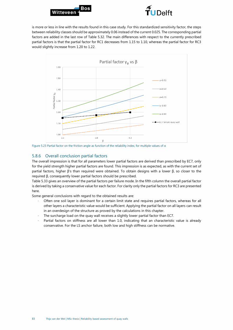
83 Thijs van der Wel | MSc thesis | Reliability based assessment of quay walls
is more or less in line with the results found in this case study. For this standardized sensitivity factor, the steps
between reliability classes should be approximately 0.06 instead of the current 0.025. The corresponding partial
factors are added in the last row of Table 5.32. The main differences with respect to the currently prescribed
partial factors is that the partial factor for RC1 decreases from 1.15 to 1.10, whereas the partial factor for RC3
would slightly increase from 1.20 to 1.22.
Figure 5.23 Partial factor on the friction angle as function of the reliability index, for multiple values of α
5.8.6 Overall conclusion partial factors
The overall impression is that for all parameters lower partial factors are derived than prescribed by EC7, only
for the yield strength higher partial factors are found. This impression is as expected, as with the current set of
partial factors, higher β’s than required were obtained. To obtain designs with a lower β, so closer to the
required β, consequently lower partial factors should be prescribed.
Table 5.33 gives an overview of the partial factors per failure mode. In the fifth column the overall partial factor
is derived by taking a conservative value for each factor. For clarity only the partial factors for RC3 are presented
here.
Some general conclusions with regard to the obtained results are:
· Often one soil layer is dominant for a certain limit state and requires partial factors, whereas for all
other layers a characteristic value would be sufficient. Applying the partial factor on all layers can result
in an overdesign of the structure as proved by the calculations in this chapter.
· The surcharge load on the quay wall receives a slightly lower partial factor than EC7.
· Partial factors on stiffness are all lower than 1.0, indicating that an characteristic value is already
conservative. For the LS anchor failure, both low and high stiffness can be normative.
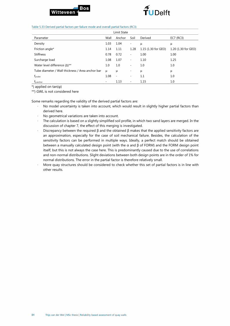
84 Thijs van der Wel | MSc thesis | Reliability based assessment of quay walls
Table 5.33 Derived partial factors per failure mode and overall partial factors (RC3)
Limit State
Parameter Wall Anchor Soil Derived EC7 (RC3)
Density 1.03 1.04 - μ μ
Friction angle* 1.14 1.11 1.28 1.15 (1.30 for GEO) 1.20 (1.30 for GEO)
Stiffness 0.78 0.72 - 1.00 1.00
Surcharge load 1.08 1.07 - 1.10 1.25
Water level difference (∆)** 1.0 1.0 - 1.0 1.0
Tube diameter / Wall thickness / Area anchor bar μ μ - μ μ
fy,tube 1.08 - - 1.1 1.0
fy,anchor - 1.13 - 1.15 1.0
*) applied on tan(φ)
**) GWL is not considered here
Some remarks regarding the validity of the derived partial factors are:
· No model uncertainty is taken into account, which would result in slightly higher partial factors than
derived here.
· No geometrical variations are taken into account.
· The calculation is based on a slightly simplified soil profile, in which two sand layers are merged. In the
discussion of chapter 7, the effect of this merging is investigated.
· Discrepancy between the required β and the obtained β makes that the applied sensitivity factors are
an approximation, especially for the case of soil mechanical failure. Besides, the calculation of the
sensitivity factors can be performed in multiple ways. Ideally, a perfect match should be obtained
between a manually calculated design point (with the α and β of FORM) and the FORM design point
itself, but this is not always the case here. This is predominantly caused due to the use of correlations
and non-normal distributions. Slight deviations between both design points are in the order of 1% for
normal distributions. The error in the partial factor is therefore relatively small.
· More quay structures should be considered to check whether this set of partial factors is in line with
other results.
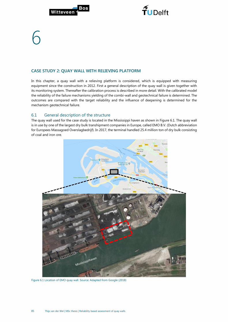
85 Thijs van der Wel | MSc thesis | Reliability based assessment of quay walls
6
CASE STUDY 2: QUAY WALL WITH RELIEVING PLATFORM
In this chapter, a quay wall with a relieving platform is considered, which is equipped with measuring
equipment since the construction in 2012. First a general description of the quay wall is given together with
its monitoring system. Thereafter the calibration process is described in more detail. With the calibrated model
the reliability of the failure mechanisms yielding of the combi-wall and geotechnical failure is determined. The
outcomes are compared with the target reliability and the influence of deepening is determined for the
mechanism geotechnical failure.
6.1 General description of the structure
The quay wall used for the case study is located in the Mississippi haven as shown in Figure 6.1. The quay wall
is in use by one of the largest dry bulk transhipment companies in Europe, called EMO B.V. (Dutch abbreviation
for Europees Massagoed Overslagbedrijf). In 2017, the terminal handled 25.4 million ton of dry bulk consisting
of coal and iron ore.
Figure 6.1 Location of EMO quay wall. Source: Adapted from Google (2018)

86 Thijs van der Wel | MSc thesis | Reliability based assessment of quay walls
The quay wall used for this case study is constructed in 2012 and has a total length of 485m. The drawing is
presented in Figure 6.2.
Figure 6.2 EMO quay wall
The quay wall is designed for a retaining height of 23.65m and consists of a concrete superstructure with
relieving platform founded on a combi-wall and Vibro piles. At the back of the concrete superstructure grout
anchors are installed. The combi-wall is installed with an inclination of 5:1 and consists of steel tubular piles
with a diameter of 1420mm with three AU20 sheet pile elements in between. The combi-wall is connected with
the superstructure by a cast iron saddle. In this way the bending moments in the superstructure are not
transferred to the combi-wall, allowing for a lighter profile.
The concrete Vibro piles are placed with an inclination as well, alternating between 4:1 and 3:1 and are thus
providing horizontal support to the superstructure. The diameter of the piles ranges between 560 and 660mm,
and the installation depth varies between NAP-24.00m and NAP-29.00m.
The most important geometric parameters are:
· Top level structure: NAP +5.0m
· Construction depth: NAP - 18.65m
· Contract depth: NAP - 16.65m
· Current depth: NAP - 17.15m
The properties of the combi-wall are given in Table 6.1.

87 Thijs van der Wel | MSc thesis | Reliability based assessment of quay walls
Table 6.1 Properties of the combi-wall
Description Symbol Value Unit
Sheet piles type AU20 -
Amount 3 -
Steel grade fy S355GP N/mm2
Tip level -22.65 m NAP
Tubular piles Outer diameter D 1420 mm
Thickness t 16 mm
Steel grade fy X65 (445 MPa) -
Pile tip level -31.0 m NAP
c.t.c. distance 3.73 m
Properties per m’ Bending stiffness EI 0.979*106 kNm2/m’
Axial stiffness EA 3.97*106 kN/m’
Weight w 2.26 kN/m/m’
Cross-sectional area A 1.892*10-2 m2/m’
Section modulus Wel 6.57*10-3 m3/m’
The specifications of the anchors are given in Table 6.2.
Table 6.2 Anchor properties
Symbol Value Unit
Angle w.r.t. horizontal 18 °
Anchor type 82.5 x 22.0mm -
Cross-sectional area A 4181 mm2
Steel grade AC 600D
Minimum yield stress fy 600 N/mm2
Minimum tensile stress 750 N/mm2
Connection with superstructure +0.9 m NAP
Top level grout body -4.35 m NAP
Length grout body 12 m
Diameter grout body 250 mm
c.t.c. distance 2.755 m
Axial stiffness per m’ EA 319*103 kN/m’
6.2 Description of the measurement program
The quay wall is equipped with fibre optic measuring sensors already in the construction phase in 2012. Most
of the sensors measure every 3 hours and send their data via a computer on location to a webserver. This
server is accessible for the Port of Rotterdam authority, who can use the measurements for asset management
and research. The sensors measure the following:
· Air pressure
· Temperature:
- Air
- Harbour water
- Ground water
· Water level:
- Harbour water.
- Ground water, 4 sensors
· Anchor strains, 4 sensors
· SAAF (Shape Accel Array/Field) (=inclinometers), 4 sensors
· DSS (Distributed Strain Sensor) to monitor the erosion below the concrete relieving platform, 2 sensors.
· Deformation bolts, 25 units (measured by Fugro BV.).

88 Thijs van der Wel | MSc thesis | Reliability based assessment of quay walls
Not all sensors measure continuously, in Table 6.3 a division is made between continuous measurements and
manual measurements. The position of the sensors in the cross section is shown in Figure 6.3, while Figure 6.4
shows the location of the sensors. The sensors for measuring the groundwater level, the anchor force and the
deformations (SAAF) are installed at four locations along the quay and are accessible for maintenance in the
corresponding pit (referred to as P1, P2, P3 and P4).
Table 6.3 Types of measurements
Continuous measurements (every 3 hours) Manual measurements
Temperature; groundwater, harbour water and near
anchorage
SAAF Inclinometers in combi-wall (19
measurements until date)
Water level; groundwater, harbour water Deformation bolts (6 measurements until date)
Anchor strains
DSS
Figure 6.3 Position of the sensors (bounded in yellow)
All these measurements over multiple years result in a huge amount of raw data, which needs to be processed
to get usable results. The raw data can be corrupted due to multiple causes:
· Power failure
· Maintenance (once every three months)
· Corroded or defect sensors
· Other causes (For example: rainwater entering the measurement pit and subsequently raising the water
level in the standpipe of the ground water level)
During the data analysis, it turned out that quite a lot of sensors are defect or corrupted, either for a small
period or forever.
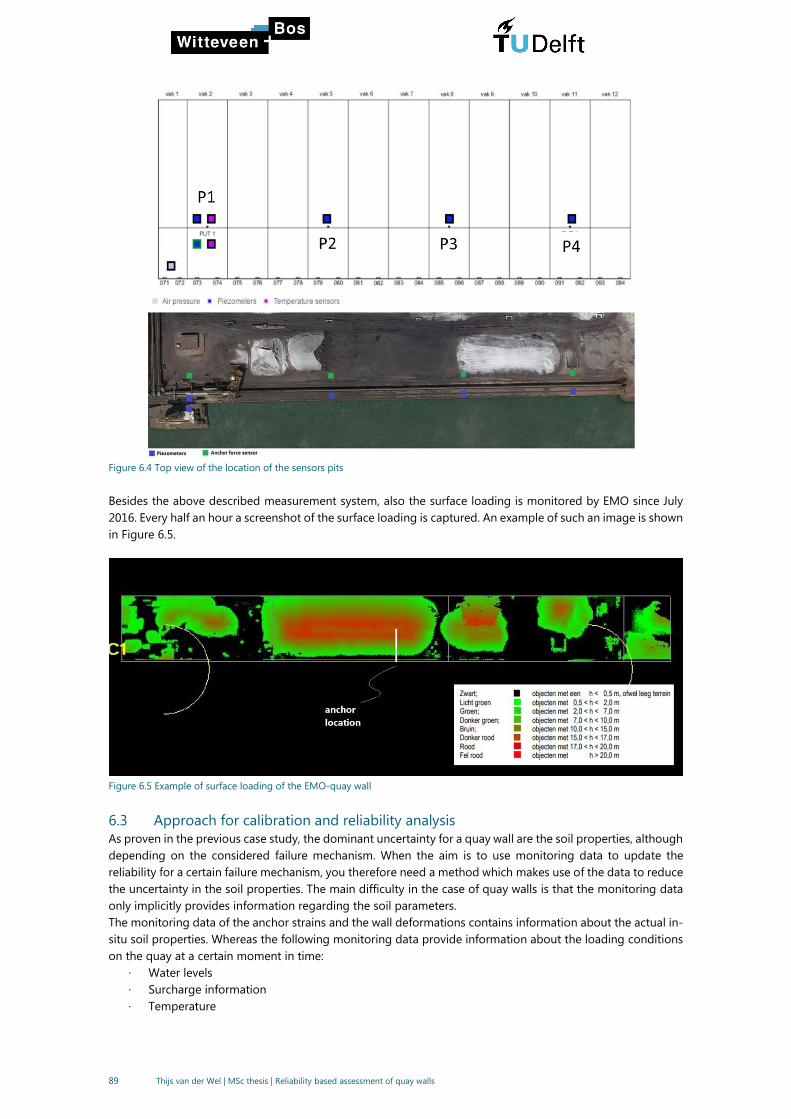
89 Thijs van der Wel | MSc thesis | Reliability based assessment of quay walls
Figure 6.4 Top view of the location of the sensors pits
Besides the above described measurement system, also the surface loading is monitored by EMO since July
2016. Every half an hour a screenshot of the surface loading is captured. An example of such an image is shown
in Figure 6.5.
Figure 6.5 Example of surface loading of the EMO-quay wall
6.3 Approach for calibration and reliability analysis
As proven in the previous case study, the dominant uncertainty for a quay wall are the soil properties, although
depending on the considered failure mechanism. When the aim is to use monitoring data to update the
reliability for a certain failure mechanism, you therefore need a method which makes use of the data to reduce
the uncertainty in the soil properties. The main difficulty in the case of quay walls is that the monitoring data
only implicitly provides information regarding the soil parameters.
The monitoring data of the anchor strains and the wall deformations contains information about the actual in-
situ soil properties. Whereas the following monitoring data provide information about the loading conditions
on the quay at a certain moment in time:
· Water levels
· Surcharge information
· Temperature
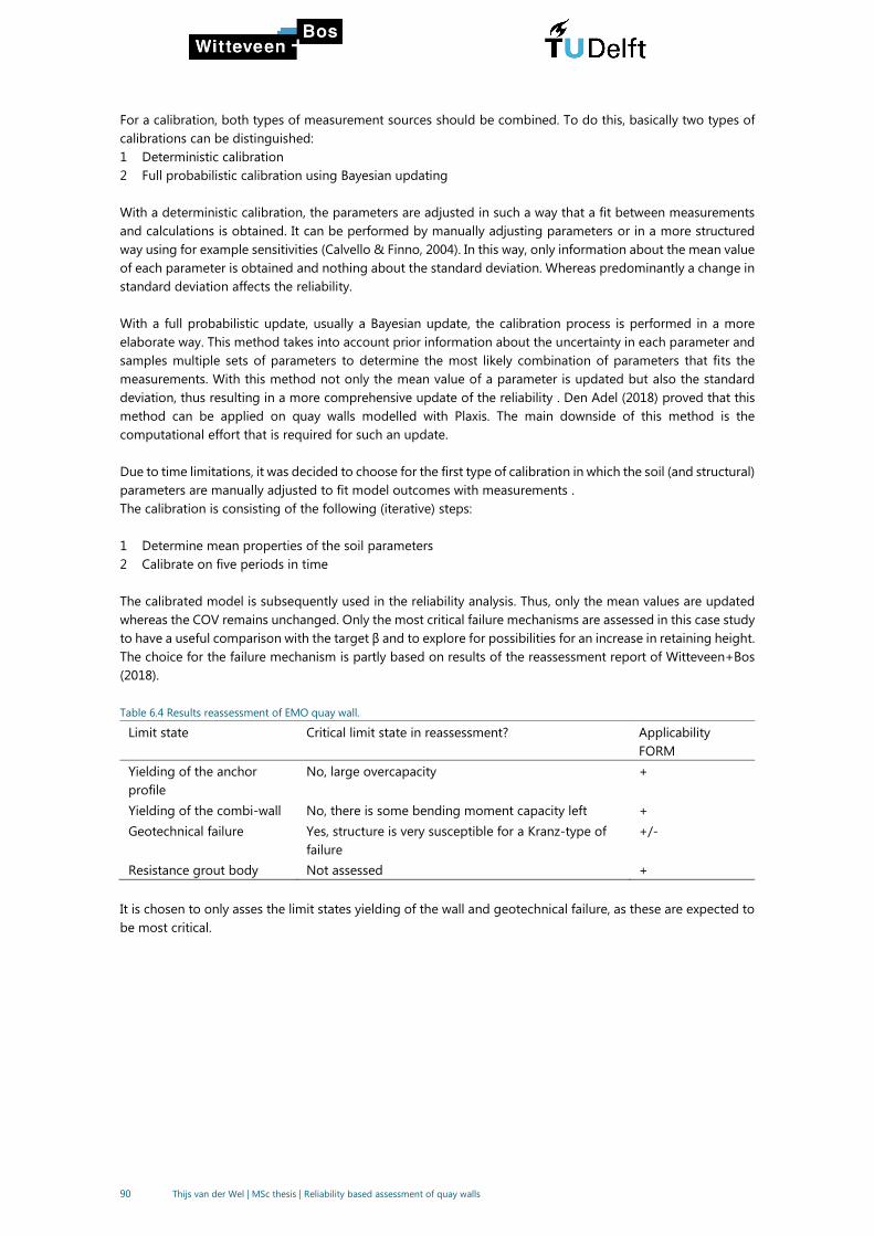
90 Thijs van der Wel | MSc thesis | Reliability based assessment of quay walls
For a calibration, both types of measurement sources should be combined. To do this, basically two types of
calibrations can be distinguished:
1 Deterministic calibration
2 Full probabilistic calibration using Bayesian updating
With a deterministic calibration, the parameters are adjusted in such a way that a fit between measurements
and calculations is obtained. It can be performed by manually adjusting parameters or in a more structured
way using for example sensitivities (Calvello & Finno, 2004). In this way, only information about the mean value
of each parameter is obtained and nothing about the standard deviation. Whereas predominantly a change in
standard deviation affects the reliability.
With a full probabilistic update, usually a Bayesian update, the calibration process is performed in a more
elaborate way. This method takes into account prior information about the uncertainty in each parameter and
samples multiple sets of parameters to determine the most likely combination of parameters that fits the
measurements. With this method not only the mean value of a parameter is updated but also the standard
deviation, thus resulting in a more comprehensive update of the reliability . Den Adel (2018) proved that this
method can be applied on quay walls modelled with Plaxis. The main downside of this method is the
computational effort that is required for such an update.
Due to time limitations, it was decided to choose for the first type of calibration in which the soil (and structural)
parameters are manually adjusted to fit model outcomes with measurements .
The calibration is consisting of the following (iterative) steps:
1 Determine mean properties of the soil parameters
2 Calibrate on five periods in time
The calibrated model is subsequently used in the reliability analysis. Thus, only the mean values are updated
whereas the COV remains unchanged. Only the most critical failure mechanisms are assessed in this case study
to have a useful comparison with the target β and to explore for possibilities for an increase in retaining height.
The choice for the failure mechanism is partly based on results of the reassessment report of Witteveen+Bos
(2018).
Table 6.4 Results reassessment of EMO quay wall.
Limit state Critical limit state in reassessment? Applicability
FORM
Yielding of the anchor
profile
No, large overcapacity +
Yielding of the combi-wall No, there is some bending moment capacity left +
Geotechnical failure Yes, structure is very susceptible for a Kranz-type of
failure
+/-
Resistance grout body Not assessed +
It is chosen to only asses the limit states yielding of the wall and geotechnical failure, as these are expected to
be most critical.

91 Thijs van der Wel | MSc thesis | Reliability based assessment of quay walls
6.4 Calibration of the model
The model is calibrated on the location of Pit 3 (P3 at Figure 6.4). This location was the most suitable because
at other locations either sensors were corrupted or loading by a large coal pile was limited due the existence
of buildings.
The soil stratification is based on the stratification used in the report of (Witteveen+Bos, 2018) instead of the
soil profile used in the original design by Volker InfraDesign (2011). The reason for this is that for the original
design the soil parameters are determined based on the several correlations between cone resistance, relative
density and friction angle. The soil parameters can therefore not be considered as characteristic values. This
makes the transformation to mean values complicated.
The soil stratification used by Witteveen+Bos is based on the soil classes defined in the NEN9997. The used
CPTs and an overview of the complete soil profile along the quay wall can be found in Appendix I.
The characteristic values of the soil parameters are given in Table 6.5. The Hardening soil parameters are given
further on in Table 6.7.
Table 6.5 Characteristic values at Pit 3
Level
[m w.r.t.
NAP]
Description Layer number
[-]
qc
[MPa]
γunsaturated
[kN/m3]
γsaturated
[kN/m3]
ϕ’
[°]
c’
[kN/m2]
5.0 Sand, moderate, top 1 10 18.0 20.0 32.5 0
-3.0 Sand, dense 2 20 19.0 21.0 35.0 0
-7.8 Clay, w. sandy,
moderate
3 2 17.0 18.0 25.0 7.5
-9.1 Sand, moderate, 2 4 22 18.0 20.0 32.5 0
-12.0 Sand, clay layers 5 21 18.1 18.7 27.5 0
-19.0 Sand, Pleistocene 6 40 19.0 21.0 35.0 0
The Plaxis model of the quay wall is shown in Figure 6.6.
Figure 6.6 Plaxis model of the quay structure
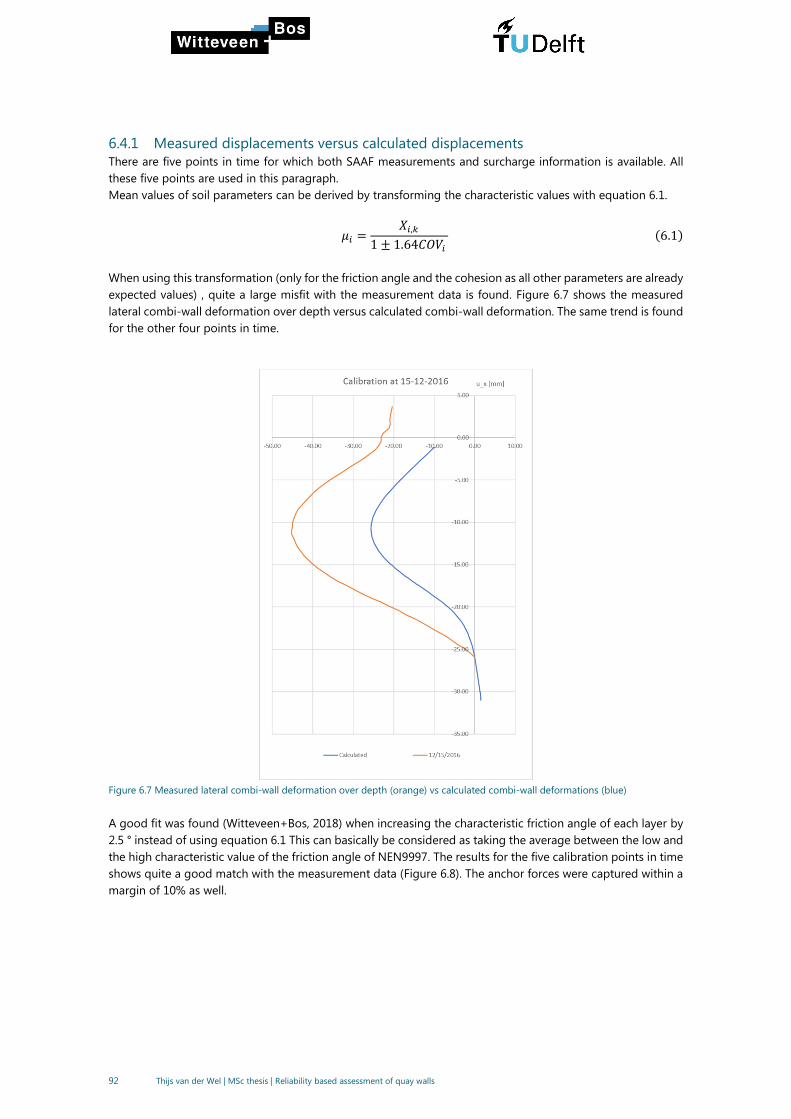
92 Thijs van der Wel | MSc thesis | Reliability based assessment of quay walls
6.4.1 Measured displacements versus calculated displacements
There are five points in time for which both SAAF measurements and surcharge information is available. All
these five points are used in this paragraph.
Mean values of soil parameters can be derived by transforming the characteristic values with equation 6.1.
𝜇𝑖 =𝑋𝑖,𝑘
1 ± 1.64𝐶𝑂𝑉𝑖(6.1)
When using this transformation (only for the friction angle and the cohesion as all other parameters are already
expected values) , quite a large misfit with the measurement data is found. Figure 6.7 shows the measured
lateral combi-wall deformation over depth versus calculated combi-wall deformation. The same trend is found
for the other four points in time.
Figure 6.7 Measured lateral combi-wall deformation over depth (orange) vs calculated combi-wall deformations (blue)
A good fit was found (Witteveen+Bos, 2018) when increasing the characteristic friction angle of each layer by
2.5 ° instead of using equation 6.1 This can basically be considered as taking the average between the low and
the high characteristic value of the friction angle of NEN9997. The results for the five calibration points in time
shows quite a good match with the measurement data (Figure 6.8). The anchor forces were captured within a
margin of 10% as well.
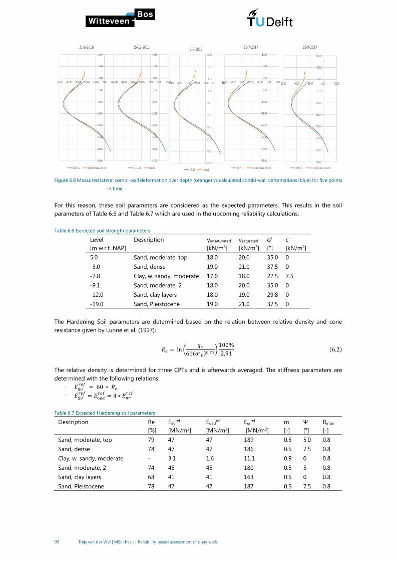
93 Thijs van der Wel | MSc thesis | Reliability based assessment of quay walls
Figure 6.8 Measured lateral combi-wall deformation over depth (orange) vs calculated combi-wall deformations (blue) for five points
in time
For this reason, these soil parameters are considered as the expected parameters. This results in the soil
parameters of Table 6.6 and Table 6.7 which are used in the upcoming reliability calculations:
Table 6.6 Expected soil strength parameters
Level
[m w.r.t. NAP]
Description γunsaturated
[kN/m3]
γsaturated
[kN/m3]
ϕ’
[°]
c’
[kN/m2]
5.0 Sand, moderate, top 18.0 20.0 35.0 0
-3.0 Sand, dense 19.0 21.0 37.5 0
-7.8 Clay, w. sandy, moderate 17.0 18.0 22.5 7.5
-9.1 Sand, moderate, 2 18.0 20.0 35.0 0
-12.0 Sand, clay layers 18.0 19.0 29.8 0
-19.0 Sand, Pleistocene 19.0 21.0 37.5 0
The Hardening Soil parameters are determined based on the relation between relative density and cone
resistance given by Lunne et al. (1997):
𝑅𝑒 = ln (𝑞𝑐
61(𝜎′𝑣)0,71)
100%
2,91(6.2)
The relative density is determined for three CPTs and is afterwards averaged. The stiffness parameters are
determined with the following relations:
· 𝐸50𝑟𝑒𝑓
= 60 ∗ 𝑅𝑒
· 𝐸50𝑟𝑒𝑓
= 𝐸𝑜𝑒𝑑𝑟𝑒𝑓
= 4 ∗ 𝐸𝑢𝑟𝑟𝑒𝑓
Table 6.7 Expected Hardening soil parameters
Description Re
[%]
E50ref
[MN/m2]
Eoedref
[MN/m2]
Eurref
[MN/m2]
m
[-]
Ψ
[°]
Rinter
[-]
Sand, moderate, top 79 47 47 189 0.5 5.0 0.8
Sand, dense 78 47 47 186 0.5 7.5 0.8
Clay, w. sandy, moderate - 3.1 1,6 11,1 0.9 0 0.8
Sand, moderate, 2 74 45 45 180 0.5 5 0.8
Sand, clay layers 68 41 41 163 0.5 0 0.8
Sand, Pleistocene 78 47 47 187 0.5 7.5 0.8
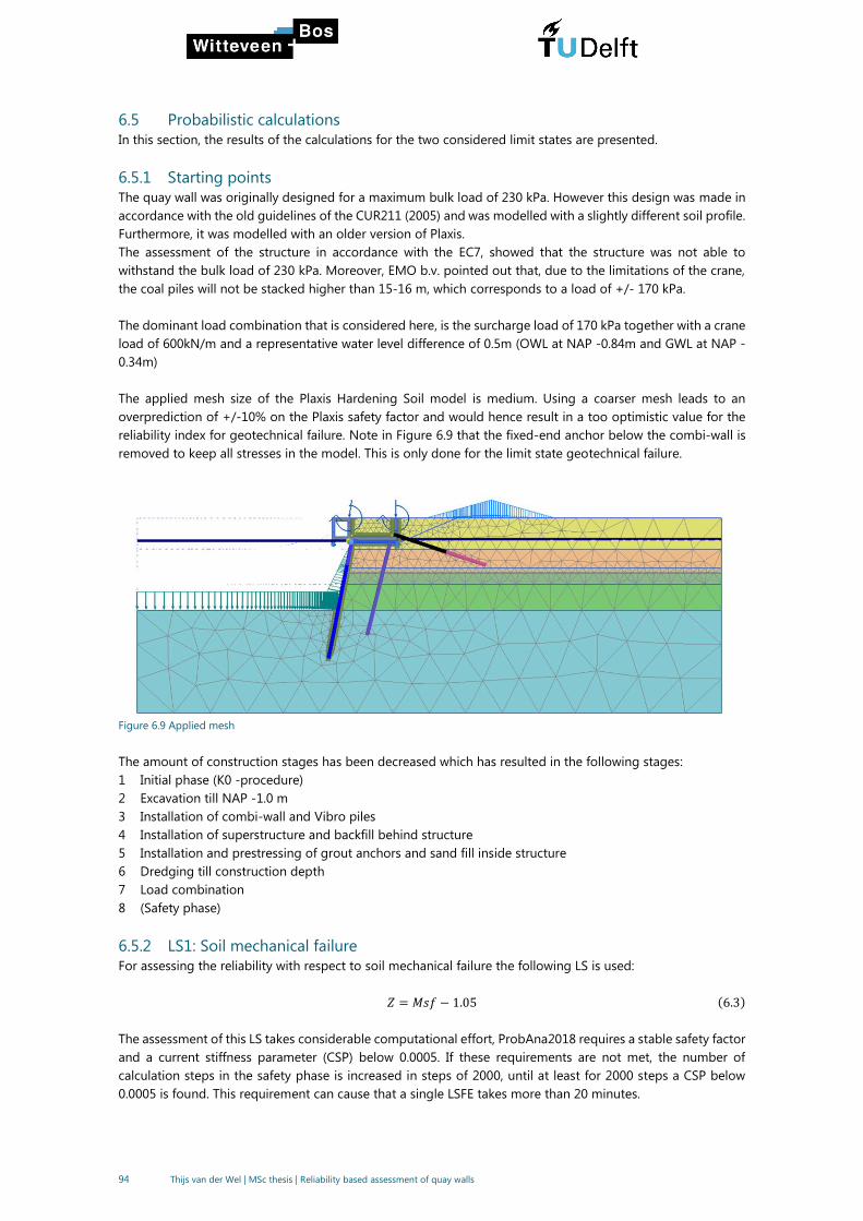
94 Thijs van der Wel | MSc thesis | Reliability based assessment of quay walls
6.5 Probabilistic calculations
In this section, the results of the calculations for the two considered limit states are presented.
6.5.1 Starting points
The quay wall was originally designed for a maximum bulk load of 230 kPa. However this design was made in
accordance with the old guidelines of the CUR211 (2005) and was modelled with a slightly different soil profile.
Furthermore, it was modelled with an older version of Plaxis.
The assessment of the structure in accordance with the EC7, showed that the structure was not able to
withstand the bulk load of 230 kPa. Moreover, EMO b.v. pointed out that, due to the limitations of the crane,
the coal piles will not be stacked higher than 15-16 m, which corresponds to a load of +/- 170 kPa.
The dominant load combination that is considered here, is the surcharge load of 170 kPa together with a crane
load of 600kN/m and a representative water level difference of 0.5m (OWL at NAP -0.84m and GWL at NAP -
0.34m)
The applied mesh size of the Plaxis Hardening Soil model is medium. Using a coarser mesh leads to an
overprediction of +/-10% on the Plaxis safety factor and would hence result in a too optimistic value for the
reliability index for geotechnical failure. Note in Figure 6.9 that the fixed-end anchor below the combi-wall is
removed to keep all stresses in the model. This is only done for the limit state geotechnical failure.
Figure 6.9 Applied mesh
The amount of construction stages has been decreased which has resulted in the following stages:
1 Initial phase (K0 -procedure)
2 Excavation till NAP -1.0 m
3 Installation of combi-wall and Vibro piles
4 Installation of superstructure and backfill behind structure
5 Installation and prestressing of grout anchors and sand fill inside structure
6 Dredging till construction depth
7 Load combination
8 (Safety phase)
6.5.2 LS1: Soil mechanical failure
For assessing the reliability with respect to soil mechanical failure the following LS is used:
𝑍 = 𝑀𝑠𝑓 − 1.05 (6.3)
The assessment of this LS takes considerable computational effort, ProbAna2018 requires a stable safety factor
and a current stiffness parameter (CSP) below 0.0005. If these requirements are not met, the number of
calculation steps in the safety phase is increased in steps of 2000, until at least for 2000 steps a CSP below
0.0005 is found. This requirement can cause that a single LSFE takes more than 20 minutes.
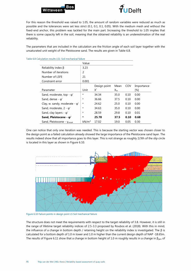
95 Thijs van der Wel | MSc thesis | Reliability based assessment of quay walls
For this reason the threshold was raised to 1.05, the amount of random variables were reduced as much as
possible and the tolerances were set less strict (0.1, 0.1, 0.1, 0.05). With the medium mesh and without the
fixed-end anchor, this problem was tackled for the main part. Increasing the threshold to 1.05 implies that
there is some capacity left in the soil, meaning that the obtained reliability is an underestimation of the real
reliability.
The parameters that are included in the calculation are the friction angle of each soil layer together with the
unsaturated unit weight of the Pleistocene sand. The results are given in Table 6.8.
Table 6.8 Calculation results LS1: Soil mechanical failure
Value
Reliability index β 3.23
Number of iterations 2
Number of LSFE 21
Constraint error 0.001
Parameter
Unit
Design point
X*
Mean
Xm
COV Importance
[%]
Sand, moderate, top - φ’ ᵒ 34.34 35.0 0.10 0.00
Sand, dense - φ’ ᵒ 36.66 37.5 0.10 0.00
Clay, w. sandy, moderate - φ’ ᵒ 24.62 25.0 0.10 0.00
Sand, moderate, 2 - φ’ ᵒ 34.63 35.0 0.10 0.00
Sand, clay layers - φ’ ᵒ 28.59 29.8 0.10 0.01
Sand, Pleistocene - φ’ ᵒ 25.78 37.5 0.10 0.68
Sand, Pleistocene - γunsat kN/m3 17.02 19.0 0.05 0.30
One can notice that only one iteration was needed. This is because the starting vector was chosen closer to
the design point as a failed calculation already showed the large importance of the Pleistocene sand layer. The
results indeed show that all importance goes to this layer. This is not strange as roughly 2/3th of the slip circle
is located in this layer as shown in Figure 6.10.
Figure 6.10 Failure points in design point LS Soil mechanical failure
The structure does not meet the requirements with respect to the target reliability of 3.8. However, it is still in
the range of lifetime target reliability indices of 2.5-3.3 proposed by Roubos et al. (2018). With this in mind,
the influence of a change in bottom depth / retaining height on the reliability index is investigated. The β is
calculated for a bottom depth of 1.0 m lower and 1.0 m higher than the current design depth of NAP -18.65m.
The results of Figure 6.11 show that a change in bottom height of 1.0 m roughly results in a change in βgeo of
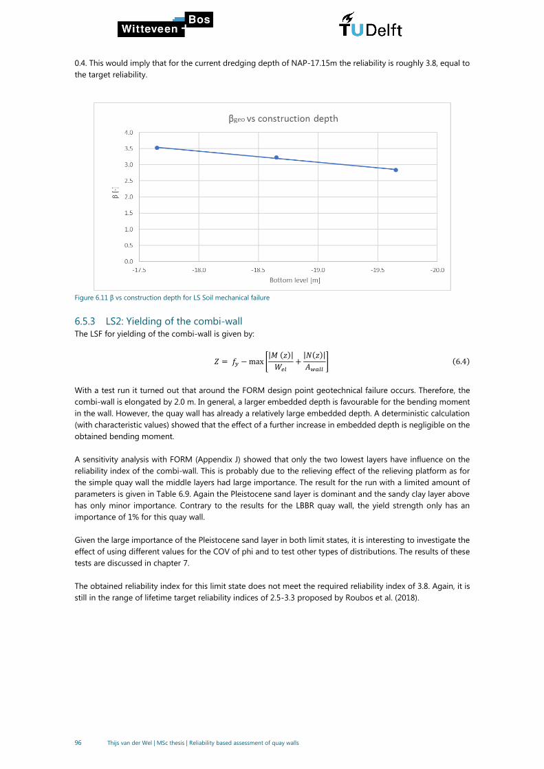
96 Thijs van der Wel | MSc thesis | Reliability based assessment of quay walls
0.4. This would imply that for the current dredging depth of NAP-17.15m the reliability is roughly 3.8, equal to
the target reliability.
Figure 6.11 β vs construction depth for LS Soil mechanical failure
6.5.3 LS2: Yielding of the combi-wall
The LSF for yielding of the combi-wall is given by:
𝑍 = 𝑓𝑦 −max [|𝑀(𝑧)|
𝑊𝑒𝑙+|𝑁(𝑧)|
𝐴𝑤𝑎𝑙𝑙] (6.4)
With a test run it turned out that around the FORM design point geotechnical failure occurs. Therefore, the
combi-wall is elongated by 2.0 m. In general, a larger embedded depth is favourable for the bending moment
in the wall. However, the quay wall has already a relatively large embedded depth. A deterministic calculation
(with characteristic values) showed that the effect of a further increase in embedded depth is negligible on the
obtained bending moment.
A sensitivity analysis with FORM (Appendix J) showed that only the two lowest layers have influence on the
reliability index of the combi-wall. This is probably due to the relieving effect of the relieving platform as for
the simple quay wall the middle layers had large importance. The result for the run with a limited amount of
parameters is given in Table 6.9. Again the Pleistocene sand layer is dominant and the sandy clay layer above
has only minor importance. Contrary to the results for the LBBR quay wall, the yield strength only has an
importance of 1% for this quay wall.
Given the large importance of the Pleistocene sand layer in both limit states, it is interesting to investigate the
effect of using different values for the COV of phi and to test other types of distributions. The results of these
tests are discussed in chapter 7.
The obtained reliability index for this limit state does not meet the required reliability index of 3.8. Again, it is
still in the range of lifetime target reliability indices of 2.5-3.3 proposed by Roubos et al. (2018).
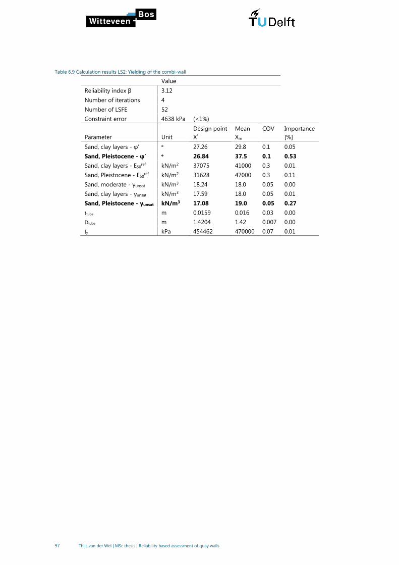
97 Thijs van der Wel | MSc thesis | Reliability based assessment of quay walls
Table 6.9 Calculation results LS2: Yielding of the combi-wall
Value
Reliability index β 3.12
Number of iterations 4
Number of LSFE 52
Constraint error 4638 kPa (<1%)
Parameter
Unit
Design point
X*
Mean
Xm
COV Importance
[%]
Sand, clay layers - φ’ ᵒ 27.26 29.8 0.1 0.05
Sand, Pleistocene - φ’ ᵒ 26.84 37.5 0.1 0.53
Sand, clay layers - E50ref kN/m2 37075 41000 0.3 0.01
Sand, Pleistocene - E50ref kN/m2 31628 47000 0.3 0.11
Sand, moderate - γunsat kN/m3 18.24 18.0 0.05 0.00
Sand, clay layers - γunsat kN/m3 17.59 18.0 0.05 0.01
Sand, Pleistocene - γunsat kN/m3 17.08 19.0 0.05 0.27
ttube m 0.0159 0.016 0.03 0.00
Dtube m 1.4204 1.42 0.007 0.00
fy kPa 454462 470000 0.07 0.01

98 Thijs van der Wel | MSc thesis | Reliability based assessment of quay walls
7
DISCUSSION
Several assumptions, simplifications and choices have been made throughout this research. It is therefore
useful to discuss their validity and to check the impact of certain assumptions on the results. The main topics
that are discussed here are:
· Influence of soil stratification
· Influence of the stochastic description of soil parameters
· Extreme values for soil parameters in FORM design points
· Influence of the use of monitoring data on the reliability
· Wider applicability of the results of both case studies
7.1 Influence of soil stratification
The results of the first case study showed that the friction angle of the loose sand layer (yellow layer in Figure
7.1) was the most important soil parameter for both yielding of the wall and yielding of the anchor bar. Herein
the soil profile was simplified by merging two sand layers to one. However, this is a conservative assumption
as in this way full dependency between both sand layers is assumed, which in reality is most likely not the case.
Figure 7.1 Applied vs original soil profile
For the applied soil profile, a reliability index β of 6.5 was found for the limit state yielding of the anchor bar.
When performing the same calculation on the original soil profile (with the two very thin clay layers left out),
the reliability index increases to 7.1. When splitting the layer even further up into a total of three equal layers,
the reliability index increases even to 8.6. This demonstrates the importance of the soil stratification in a
reliability analysis and raises questions about how many independent layers need to be modelled. Literature
(e.g. Phoon and Kulhawy (1999)) prescribe a vertical scale of fluctuation in the range of 2 to 6 m, which implies
that soil properties over a larger vertical distance are not correlated anymore. This would suggest that layers
should not be thicker than +/-6 m. This is in large contrast with the thickness of the layers in both case studies,
as layers with a thickness of 15 to 20m have been used.
7.2 Influence of the stochastic description of soil parameters
Relevant to this topic is the magnitude of the COV of the friction angle. In this research, for every layer the
same value of 0.10 was applied independently of the layer thickness. CUR-C135 (2008) stated that the COV
value given in NEN9997 should be interpreted as a spatially-averaged value. However, as already discussed in

99 Thijs van der Wel | MSc thesis | Reliability based assessment of quay walls
chapter 4, the larger the vertical extent of a layer together with the vertical extent of a failure mechanism, the
more spatial averaging is applicable (Schneider & Schneider, 2013). Thus in theory, the COV depends on the
layer thickness and the vertical extent of the failure mechanism. This is an attractive concept in terms of
reliability, but is considered doubtful by research of Ching et al. (2016) when using for a problem with
homogeneous spatial-averaged soil layers in combination with reliability-based design. Nevertheless, it is still
a topic that requires more attention.
Besides the discussion on the applicability of spatial-averaging, also the discussion on the choice for the
friction angle is interesting to consider. With triaxial testing, three different value for the friction angle are
distinguished (Figure 7.2) :
4 Friction angle at a an axial strain of 2%
5 Friction angle at a an axial strain of 5%
6 Peak friction angle
Figure 7.2 Friction angle vs axial strain. Source: CUR166 (2012)
In ULS calculations it is considered safe to use the friction angle belonging to a strain of 5%. Using the peak
friction angle is also possible, but can be considered unconservative in case of layered soil. Differences in soil
types can cause that certain layers reach failure earlier than others, causing that not all layers are at the same
time on their peak strength (CUR166, 2012). When considering the research by Huijzer (1996) in which the
triaxial test results for the Port of Rotterdam are described, a trend is visible in which the uncertainty in the
friction angle decreases with increasing strain. The results for two layers of importance for the considered case
studies in this thesis, are given in Table 7.1. It clearly shows a decrease in COV of 0.14 for 2% strain to ultimately
0.04 in case of maximum/peak friction angle. Furthermore, these values represent the point-to-point variation,
implying that the spatially averaged variation is even lower.
Table 7.1 Triaxial test results. Source: Huijzer (1996)
Holocene sand (NAP - 5m until NAP -20m) Pleistocene sand (> NAP -20 m )
Mean COV Mean COV
φ’ 2% 28.0 0.14 30.4 0.14
φ’ 5% 34.0 0.08 34.8 0.07
φ’max 35.9 0.04 36.2 0.04
The COV at 5% strain for Pleistocene sand is lower than the currently applied value of 0.10. Given the large
importance of this layer in the limit state geotechnical failure for the EMO quay wall, it is interesting to
investigate the influence of different values for COV on the reliability index of this limit state. Besides the
already performed calculations for COV = 0.10 also calculations for COV values of 0.075 and 0.05 are performed
and shown in Figure 7.3. The figure shows a significant increase in reliability index from 3.2 (COV =0.10) to 5.4
(COV = 0.05). This shows the importance of the choice for an appropriate value of COV.

100 Thijs van der Wel | MSc thesis | Reliability based assessment of quay walls
Figure 7.3 Influence of COV of βgeo of the EMO quay wall
7.3 Extreme values for soil parameters in FORM design points
Besides the discussion about the magnitude of the COV of the friction angle, also the validity of the normal
distribution for extreme values of soil properties can be questioned. Sometimes a single soil parameter is
completely dominant for the reliability of the considered limit state. A combination of a high sensitivity factor
and high reliability index can cause that the FORM design point for the friction angle of the loose sand layer
(yellow layer in Figure 7.1) reaches a value of 17 ° or even lower. It can be questioned whether it is physically
possible for such a large sand layer (although mixed with clay) to reach such a low spatially averaged value.
Triaxial test results of the database of Gemeentewerken Rotterdam (2003), which are shown in Figure 7.4, give
an indication of the lower bound in test results.
Figure 7.4 Triaxial test results
The unit weight of soil can be determined reasonably accurate, and therefore based on the unit weight, a lower
bound for the friction angle could be estimated. The problem then shifts to what the ultimate lower bound for
the unit weight of a certain layer should be. For a saturated unit weight larger than 17 kN/m3 no values below
+/-20° can be found, whereas layer averaging is not even considered here.
To see the influence of a lower bound on the reliability index, for illustrational purposes a lower bound of 25°
for the friction angle of the Pleistocene sand layer (which has a γsat of about 21 kN/m3) is assumed and is

101 Thijs van der Wel | MSc thesis | Reliability based assessment of quay walls
described by a shifted lognormal distribution (see Figure 7.5) . A truncated normal distribution could also be
used but leads sometimes to convergence errors with FORM.
Figure 7.5 Lognormal distribution for φ’ Pleistocene sand
The lognormal distribution is applied in the LS geotechnical failure of the EMO-quay wall. Compared to the
results obtained with a regular normal distribution the reliability index increases from 3.2 to 5.0. The results of
this run are shown in Table 7.2. Although it is only a hypothetical example, it illustrates the importance of the
choice of the distribution. Especially for the Maasvlakte, where the soil profile is in general well known, the use
of different types of distributions is worthwhile to further investigate.
Table 7.2 Results for geotechnical failure EMO with lognormal distribution for φ’ Pleistocene sand
Value
Reliability index β 5.0
Number of iterations 2
Number of LSFE 27
Parameter
Unit
Design point
X*
Mean
Xm
COV Importance
[%]
Sand, moderate, top - φ’ ᵒ 32.93 35.0 0.10 0.01
Sand, dense - φ’ ᵒ 35.47 37.5 0.10 0.01
Clay, w. sandy, moderate - φ’ ᵒ 24.01 25.0 0.10 0.00
Sand, moderate, 2 - φ’ ᵒ 32.67 35.0 0.10 0.01
Sand, clay layers - φ’ ᵒ 25.72 29.8 0.10 0.05
Sand, Pleistocene - φ’ ᵒ 28.48 37.5 0.10 0.46
Sand, Pleistocene - γunsat kN/m3 15.40 19.0 0.05 0.37
Sand, Pleistocene - E50ref kN/m2 27614 48000 0.30 0.08
Surcharge load 1 (Left part of coal pile) kN/m -173 -170 0.05 0.00
Surcharge load 2 (Right part of coal pile) kN/m -173 -170 0.05 0.00
7.4 Influence of the use of monitoring data on the reliability Until now the reliability of the EMO quay wall has only been determined for the calibrated model. Monitoring
data is not available for every quay wall, therefore it is useful to investigate how large the impact of a calibration
on the reliability can be. The main finding for the investigated case study was that the Pleistocene sand layer
has the largest influence on the reliability. In case no calibration would be performed, the mean value of the
friction angle of this layer would be taken at 41.9° (using equation 6.1) instead of the currently used value of
37.5°. This is roughly a difference of one standard deviation. This is a major difference what will largely affect
the reliability index. Therefore, it can be expected that for the non-calibrated model, the reliability index for

102 Thijs van der Wel | MSc thesis | Reliability based assessment of quay walls
both failure mechanisms is around one point higher. The results of the calculations for the non-calibrated
design, given in Table 7.3, indeed shows that the reliability increases with 0.9 for both failure mechanisms. The
parameters used for the non-calibrated together with the obtained FORM output are given in Appendix K.
Table 7.3 Comparison between the reliability index for the calibrated and the non-calibrated design
Non-calibrated Calibrated
Soil mechanical failure 4.1 3.2
Yielding of the combi-wall 4.0 3.1
So for this specific case study holds that the use of monitoring data is not ‘rewarding’ in terms of increase in
reliability. As it concerns only one case study, it is not possible to draw sound conclusions about whether this
will also be the case for other quay walls. It might be expected however, that also in other cases a mean friction
angle of 41.9° (corresponding to a characteristic value of 35° for dense sand in NEN9997) will not be measured
in reality.
It is also important to note that in the initial design of the contractor, optimistic soil conditions were used,
resulting an optimistic design. This is a possible explanation for the low reliability indices that were found and
the large difference between the calibrated and the non-calibrated design.
Besides, it’s good to mention that with the calibration only the mean values were updated. In case of a full-
probabilistic update/calibration, also the standard deviation of each parameter is adjusted. Even in case higher
displacements are measured than expected based on prior knowledge, the standard deviation of parameters
still decreases due to fact that extra knowledge about the problem is attained. A decrease in standard deviation
implies an increase in reliability index. So, If this would be applied here, the reliability would have turned out
higher than calculated here.
7.5 Wider applicability of the results of both case studies The results of both case studies showed deviating results for the reliability index and importance of parameters
for the considered limit states. For the simple quay wall, the obtained reliability indices were in all cases higher
than the target reliability, whereas for the quay wall with relieving platform the opposite was valid. This
difference can be explained by the fact that it concerns different type of quay structures and different soil
conditions. Furthermore, whether optimistic or pessimistic choices were made in the design, also influences
the reliability. It is therefore not directly possible to generalize the findings of both case studies. However,
considering the results from this thesis together with results obtained in previous probabilistic studies to quay
walls, similarities can be noticed with respect to the importance of certain soil layers and soil parameters. In
almost all cases the soil parameters have the most impact, followed by the structural properties.
Up to a certain degree, it can therefore be expected that for structures with almost the same composition and
similar sandy soil conditions, the reliability will be in the same order of magnitude.
103 Thijs van der Wel | MSc thesis | Reliability based assessment of quay walls
8
CONCLUSIONS AND RECOMMENDATIONS
In this chapter, the results of this research are discussed, followed by recommendations on the applicability
and recommendations for further research. The objectives of this research were:
1 Establishing the actual reliability index of a quay wall in operation.
2 Exploring possibilities for an increase in retaining height, making use of probabilistic calculations.
3 Verifying the partial factors of the current design guidelines.
8.1 Conclusions
Four research questions have been set up at the start of this research. Following, each of them will be answered
respectively. Besides this, more general conclusions are drawn about the applied methods and the obtained
results.
1 What are the most suitable probabilistic methods to determine the reliability of a quay wall modelled
with FEM?
In this thesis, the reliability of four failure mechanisms of quay walls has been investigated. These failure
mechanisms were respectively: yielding of the combi-wall, yielding of the anchor bar, shear failure of the grout
body and soil mechanical failure. By means of a literature review, the First Order Reliability Method (FORM) is
considered to be the most suitable reliability method for assessing the Limit State Functions of these
mechanisms. The main reason for this, is that the computational time using this method is much shorter
compared to level III methods like Directional Sampling and Crude Monte Carlo simulation. With FORM, the
calculation time is ranging from a few hours up to two days. The main disadvantage of FORM is its decrease
in accuracy when using non-normal distributions and non-linear limit states. As this is the case in this thesis,
the obtained failure probabilities are an approximation of the exact failure probability.
The probabilistic module ProbAna has been used for the coupling between the FORM-algorithms from the
library of OpenTURNS and the Hardening Soil model of Plaxis. Two versions of ProbAna were used during the
research, the second version is referred to as ProbAna2018. In the remainder of this chapter, conclusions about
the applicability of FORM are referring to this version.
Based on the experience gathered during this research, it is concluded that for failure of the structural
elements, FORM performed reasonably well. In most cases, the design point was reached within an error
margin of 1% on all error types and was obtained after less than 10 iterations. Failed calculations were mainly
caused by either soil body collapse, or were due to input restrictions in Plaxis on the values of 𝐸𝑜𝑒𝑑 and 𝐾0𝑛𝑐.
To limit the occurrence of this second error, the ratio between E50 and Eoed, was slightly adapted from 1 : 1 to
approximately 1 : 0.8 for the stiffness parameters that caused this problem. Soil body collapse was a problem
that occurred for the quay wall with relieving platform, during the evaluation of failure of the combi-wall. This
was solved by increasing the embedded depth of the combi-wall.
Regarding the limit state soil mechanical failure, difficulties were encountered in reaching a clearly defined
safety factor using the phi-c reduction method. Furthermore, the mesh of the model needs to be finer than
for the assessment of structural elements. Therefore, the computational effort for this limit state is significantly
larger than for the other limit states. A preliminary calculation to find the direction of the design point and

104 Thijs van der Wel | MSc thesis | Reliability based assessment of quay walls
thus the starting vector, highly reduces the calculation time. Due to the extra measures in ProbAna to increase
the robustness for this limit state, it can be concluded that FORM is also applicable for this limit state.
2 What are the most sensitive parameters for each failure mode and for the overall system reliability?
In general, it can be concluded that, given a specified design, the uncertainty in the soil parameters have the
largest influence on the reliability of the considered failure mechanisms. Of the three types of soil parameters
included within this research (E50ref , φ’, γ), the friction angle has the most influence in the investigated limit
states. Time-dependent loads such as water level differences and surcharge loads are only occasionally
included in the evaluations as they turned out to be of minor influence on the reliability.
Findings simple quay wall (double anchored combi-wall)
From the probabilistic calculations with respect to yielding of both the combi-wall and the anchor, it can be
concluded that the friction angle of the loosely packed sand layer together with the yield strength have a large
influence on the reliability. The obtained reliability indices (Table 8.1) for the as-built structure are all higher
than the target reliability of 4.3. This was partly caused by the low unity check for the combi-wall. The results
of Table 8.1 were obtained with calculations in which only the soil parameters were considered random.
Table 8.1 Obtained reliability indices for the as-built quay wall (RC3: βtarget=4.3)
Limit state Yielding combi-wall Yielding anchor bar Soil mechanical failure
β 6.5 6.5 7.9
For a slightly adjusted quay wall design with unity checks around 1.0, extensive calculations have been
performed, including variable loads and structural parameters as random variables. Reliability indices (Table
8.2) obtained for this design show that also for this structure there is some overcapacity.
Table 8.2 Obtained reliability indices for the adjusted quay wall (RC3: βtarget=4.3)
Limit state Yielding combi-wall Yielding anchor bar Resistance grout body
β 5.7 5.3 4.9
Findings quay wall with relieving platform
The two failure mechanisms evaluated for the quay wall with relieving platform are yielding of the wall and
soil mechanical failure. For both limit states, the friction angle of the dense Pleistocene sand layer is of major
influence on the reliability. Most probably the relieving platform causes that only the deeper soil layers have
influence on the reliability with respect to failure of the combi-wall. In contrast to the results of the simple
quay wall, the yield strength was only of minor influence in the limit state.
Table 8.3 Obtained reliability indices for the as-built quay wall (RC2: βtarget=3.8)
Limit state Yielding combi-wall Soil mechanical failure
β 3.1 3.2
The obtained reliability indices (Table 8.3) for the two failure mechanisms are lower than the target reliability
of 3.8. It is important to note that in the initial design by the contractor, optimistic soil conditions were used,
especially for the Pleistocene sand layer, which might have resulted in a too optimistic design. A second
explanation is that in this case one soil parameter is extremely dominant with respect to the reliability. A semi-
probabilistic design method is not developed for such an extreme case. This can cause that the reliability index
is lower than the target reliability index.
3 How can monitoring data be used for model calibration and parameter distribution updating ?
There is still quite some uncertainty in the modelling of the behaviour of a quay wall. The monitoring data,
consisting of anchor strains, wall deformations, water levels and temperature, helped with reducing the
uncertainty in the modelling of the quay wall with relieving platform. A good fit was found between the
measured and the calculated combi-wall deformations and anchor forces by performing a manual calibration.
The obtained set of soil parameters were used as mean values in the probabilistic calculations. The calibration
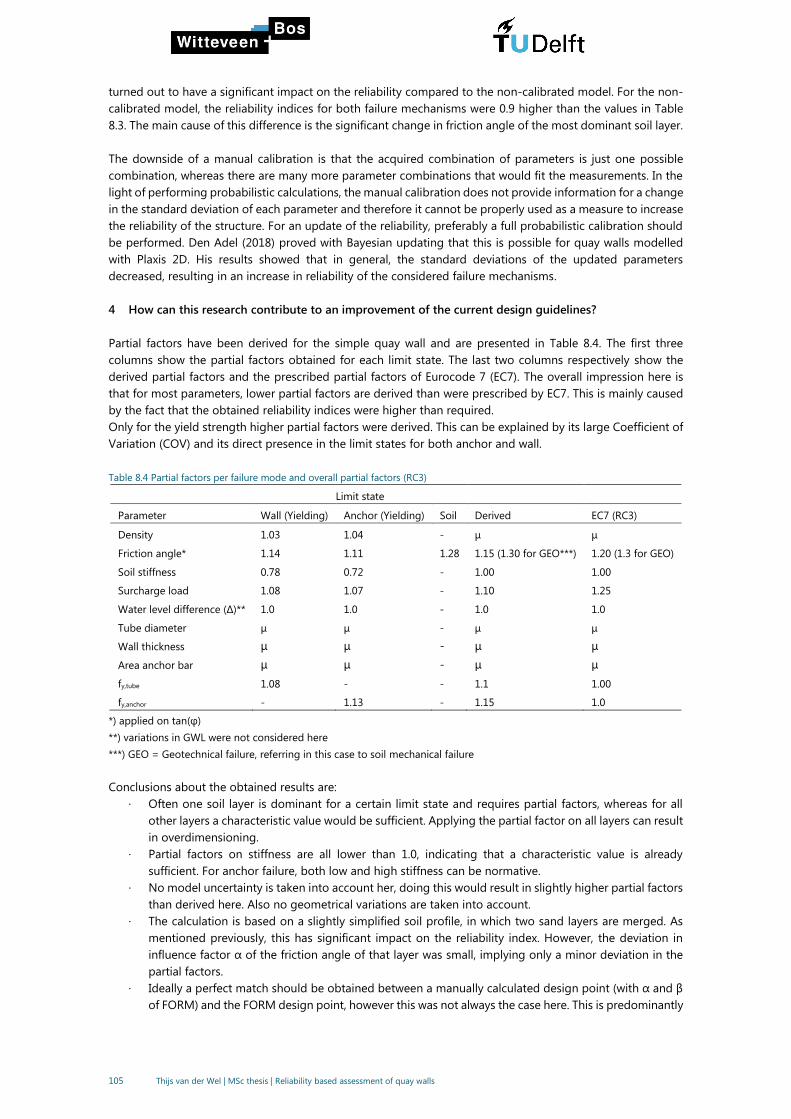
105 Thijs van der Wel | MSc thesis | Reliability based assessment of quay walls
turned out to have a significant impact on the reliability compared to the non-calibrated model. For the non-
calibrated model, the reliability indices for both failure mechanisms were 0.9 higher than the values in Table
8.3. The main cause of this difference is the significant change in friction angle of the most dominant soil layer.
The downside of a manual calibration is that the acquired combination of parameters is just one possible
combination, whereas there are many more parameter combinations that would fit the measurements. In the
light of performing probabilistic calculations, the manual calibration does not provide information for a change
in the standard deviation of each parameter and therefore it cannot be properly used as a measure to increase
the reliability of the structure. For an update of the reliability, preferably a full probabilistic calibration should
be performed. Den Adel (2018) proved with Bayesian updating that this is possible for quay walls modelled
with Plaxis 2D. His results showed that in general, the standard deviations of the updated parameters
decreased, resulting in an increase in reliability of the considered failure mechanisms.
4 How can this research contribute to an improvement of the current design guidelines?
Partial factors have been derived for the simple quay wall and are presented in Table 8.4. The first three
columns show the partial factors obtained for each limit state. The last two columns respectively show the
derived partial factors and the prescribed partial factors of Eurocode 7 (EC7). The overall impression here is
that for most parameters, lower partial factors are derived than were prescribed by EC7. This is mainly caused
by the fact that the obtained reliability indices were higher than required.
Only for the yield strength higher partial factors were derived. This can be explained by its large Coefficient of
Variation (COV) and its direct presence in the limit states for both anchor and wall.
Table 8.4 Partial factors per failure mode and overall partial factors (RC3)
Limit state
Parameter Wall (Yielding) Anchor (Yielding) Soil Derived EC7 (RC3)
Density 1.03 1.04 - μ μ
Friction angle* 1.14 1.11 1.28 1.15 (1.30 for GEO***) 1.20 (1.3 for GEO)
Soil stiffness 0.78 0.72 - 1.00 1.00
Surcharge load 1.08 1.07 - 1.10 1.25
Water level difference (∆)** 1.0 1.0 - 1.0 1.0
Tube diameter μ μ - μ μ
Wall thickness μ μ - μ μ
Area anchor bar μ μ - μ μ
fy,tube 1.08 - - 1.1 1.00
fy,anchor - 1.13 - 1.15 1.0
*) applied on tan(φ)
**) variations in GWL were not considered here
***) GEO = Geotechnical failure, referring in this case to soil mechanical failure
Conclusions about the obtained results are:
· Often one soil layer is dominant for a certain limit state and requires partial factors, whereas for all
other layers a characteristic value would be sufficient. Applying the partial factor on all layers can result
in overdimensioning.
· Partial factors on stiffness are all lower than 1.0, indicating that a characteristic value is already
sufficient. For anchor failure, both low and high stiffness can be normative.
· No model uncertainty is taken into account her, doing this would result in slightly higher partial factors
than derived here. Also no geometrical variations are taken into account.
· The calculation is based on a slightly simplified soil profile, in which two sand layers are merged. As
mentioned previously, this has significant impact on the reliability index. However, the deviation in
influence factor α of the friction angle of that layer was small, implying only a minor deviation in the
partial factors.
· Ideally a perfect match should be obtained between a manually calculated design point (with α and β
of FORM) and the FORM design point, however this was not always the case here. This is predominantly

106 Thijs van der Wel | MSc thesis | Reliability based assessment of quay walls
due to the use of correlations and non-normal distributions. Slight deviations between both design
points are in the order of 1%. The error in the partial factor is therefore relatively small.
8.2 Recommendations
The main recommendations for further research are presented below.
Recommendations on model input
- The probabilistic calculations showed that often one soil layer is dominant for the reliability. In case of a
high reliability index, the parameters of this layer are thus reduced to extreme low values for the design
point, especially for the friction angle. It can be questioned whether this design point is physically realistic
and whether the normal distribution is still valid for such extremes. Triaxial test results seem to show a
lower bound given a certain unit weight. Probably a (shifted) lognormal distribution or a truncated normal
distribution are more suitable, as with these distributions a lower bound can be set. Therefore research
should be performed focussing on finding the possible lower bound for separate soil types. This might be
beneficial for the reliability index.
- Soil stratification has a large influence on the reliability. Still not much guidance is available on how many
(independent) soil layers should be used in a probabilistic calculation and on how spatial averaging is
related to this. For all failure mechanisms, soil types and layer thicknesses, the same values for COV are
used in general. In theory, the spatially averaged COV largely depends on the vertical extent of the failure
domain and the vertical scale of fluctuation of the soil. This would imply case- and failure mode specific
COV values. This concept needs to be further looked into, as a lower COV would result in lower partial
factors and higher reliability indices.
- The stochastic distribution of the grout pile class factor 𝛼𝑡 has been estimated in this thesis, as in the
literature no information was found on this. As this parameter has a major influence on the reliability of
the grout body, it is recommended to collect data of quality control checks and failure tests on grout
bodies on a systematic basis to get a better insight into the stochastic nature of the factor 𝛼𝑡.
Recommendations on the use of probabilistic methods
- The applicability of FORM coupled with Plaxis for the case of quay walls, has only been verified by Teixeira
et al. (2015) using Directional Sampling. To get a better insight into the accuracy of the results of FORM,
more calculations with level III methods should be performed.
- For simple quay walls, probabilistic calculations can be performed relatively quickly. In the first stages of a
design, it could therefore be very useful to perform probabilistic calculations as it gives insight into the
parameters that are most influential. This can be used to increase the amount of tests on a specific soil
layer.
- Information about the applied FORM algorithms of OpenTURNS is very scarce. It took quite some effort
to exactly understand the working of the line search algorithm, and to find the most optimal settings for
convergence. It would take much less time for new people to get familiar with FORM or other probabilistic
methods if there would be a platform to share experience and knowledge.
Recommendations on partial factors
- The tubular piles of the combi-wall in both case studies are piles of class 4, which means they are
susceptible for buckling before the yield limit in the outer fibre is reached. This failure mechanism is not
addressed here. Therefore, it is advised to perform probabilistic calculations for this failure mechanism to
check whether this results in different partial factors.
- In this research, partial factors are derived on only one quay wall. More quay structures, with different soil
stratifications, should be considered to check whether the derived set of partial factors also holds for quay
walls in different soil conditions.
- More quay structures, with similar soil stratifications, should be considered to check whether layer- and
limit state specific partial factors could be defined for quay walls in the Port of Rotterdam. This would result
in a more optimal design.

107 Thijs van der Wel | MSc thesis | Reliability based assessment of quay walls

108 Thijs van der Wel | MSc thesis | Reliability based assessment of quay walls
REFERENCES
Acécon. (2015). Rapportage bezwijkproeven op zelfborende groutinjectiepalen.
Andrianov, G., Burriel, S., Cambier, S., Dutfoy, A., Dutka-Malen, I., De Rocquigny, E., . . .
Mangeant, F. (2007). Open TURNS, an open source initiative to Treat Uncertainties,
Risks’ N Statistics in a structured industrial approach. Paper presented at the
Proceedings of the ESREL’2007 Safety and Reliability Conference, Stavenger:
Norway.
Bach, D. (2014). Reliability-based design and quality control of bored piles. PhD Thesis,
Delft University of Technology
Baecher, G. B., & Christian, J. T. (2003). Reliability and Statistics in Geotechnical
Engineering. Chichester: Wiley.
Brinkgreve, R. B. J., & Laera, A. (2017). Probabilistic analysis.
Calle, K. O. F., & Spierenburg, S. (1991). Veiligheid van damwandconstructies,
onderzoeksrapportage deel I, Rapportnr. CO-316980/12. Grondmechanica Delft
Calvello, M., & Finno, R. J. (2004). Selecting parameters to optimize in model calibration
by inverse analysis. Computers and Geotechnics, 31(5), 410-424.
Ching, J., Hu, Y.-G., & Phoon, K.-K. (2016). On characterizing spatially variable soil shear
strength using spatial average. Probabilistic engineering mechanics., 45, 31-43.
CUR166. (2012). Damwandconstructies, deel 1: CUR Bouw & Infra.
CUR211. (2005). Handbook Quay walls. Gouda, The Netherlands: CUR.
CUR211. (2013). Quay walls, 2nd edition. Leiden, The Netherlands: SBRCURnet.
CUR236. (2011). Ankerpalen.
CUR-C135. (2008). Van onzekerheid naar betrouwbaarheid; Handreiking voor geotechnisch
ontwerpers. Gouda, The Netherlands
de Gijt, J. G. (2010). A history of quay walls. PhD Thesis, Delft University of Technology
de Grave, P. (2002). Validatie van partiële factoren uit “Probabilistische analyse
damwandconstructies”. MSc Thesis, Delft University of Technology
Den Adel, N. (2018). Load testing of a quay wall. MSc Thesis, Delft University of
Technology Delft.
Gemeentewerken Rotterdam. (2003). Alle triaxiaal proeven Rotterdam.
Google (Cartographer). (2018). Google Earth. Retrieved from
https://earth.google.com/web/
Griffiths, D. V., & Fenton, G. A. (2007). Probabilistic methods in geotechnical engineering:
SpringerWienNewYork.
Hasofer, A. M., & Lind, N. C. (1974). An exact and invariant first order reliabilty format.
Journal of the Engineering Mechanics division, 111-121.
Havinga, H. (2004). Dossier Probabilistische berekeningen, onderdeel 7.1Bc. Delft
Hicks, M. A. (2013). An explanation of characteristic values of soil properties in Eurocode
7. In In Advances in Soil Mechanics and Geotechnical Engineering (pp. 36-45).
Amsterdam: IOS Press.
Huijzer, G. P. (1996). Eindrapport probabilistische analyse damwandconstructies,
Rapportnummer 94-168/B.
JCSS. (2006). JCSS Probabilistic Model Code, Section 3.7: Soil properties.
Jonkman, S. N., Steenbergen, R. D. J. M., Morales-Nápoles, O., Vrouwenvelder, A. C. W.
M., & Vrijling, J. K. (2016). Probabilistic Design: Risk and Reliability Analysis in Civil
Engineering. Delft.
Lemaire, M. (2009). Structural reliability. London: ISTE Ltd.
109 Thijs van der Wel | MSc thesis | Reliability based assessment of quay walls
Manoj, N. R. (2017). Reliability based Ultimate Limit State Design in Finite Elements and
compliance with Eurocode7. MSc Thesis, Deflt University of Technology.
NEN-EN 1990. (2002). Eurocode - Basis of structural design. In.
NEN-EN 10219-2. (2006). Cold formed welded structural hollow sections of non-alloy
and fine grain steels - Part 2: Tolerances, dimensions and sectional properties. In.
NEN 9997. (2017). Geotechnical design of structures. In.
OpenTURNS. (2016). OpenTURNS 1.7 Reference Guide. Retrieved from
http://autobuilder.openturns.org/openturns/tag/v1.8rc1/doc/commit/3b92f16bd
65f582da0e34284f08bd27314ad5a53/squeeze-x86_64-doc/html/ReferenceGuide/
Ou, C.-Y. (2013). Deep Excavation, Theory and Practice. Tapei, Taiwan: Taylor & Francis
Group.
Peters, D. J., Sadowski, A., Rotter, M., & Taras, A. (2017). Calibration of Eurocode design
models of thin-walled cylinder under bending with full scale tests. Paper presented
at the EUROSTEEL 2017.
Phoon, K. K., & Kulhawy, F. H. (1999). Evaluation of geotechnical property variability.
Canadian Geotechnical Journal, 36, 625 – 639.
Plaxis. (2017). Material Models Manual.
Port of Rotterdam. (n.d.). Rotterdam's Port development. Retrieved from
https://www.portofrotterdam.com/nl/files/history-port-of-rotterdampng
Powell, M. J. D. (1994). A direct search optimization method that models the objective
and constraint functinos by linear interpolation. In S. Gomez & J.-P. Hennart
(Eds.), Advances in Optimization and Numerical Analysis (pp. 51-67): Springer.
Rippi, A. (2015). Structural reliability analysis of a dike with a sheet pile wall: Coupling
Reliability methods with Finite Elements. MSc Thesis, Delft University of
Technology
Roubos, A. A., Steenbergen, R. D. J. M., Schweckendiek, T., & Jonkman, S. N. (2018). Risk-
based target reliability indices for quay walls. Structural Safety, 75, 89-109.
Schneider, H. R., & Schneider, M. A. (2013). Dealing with Uncertainties in EC7. In P. Arnold
(Ed.), Modern Geotechnical Design Codes of Practice (pp. 87-100). Amsterdam:
IOS-Press.
Schrijver, I. J. M. (2016). Reliability of flexible dolphins. MSc Thesis, Delft University of
Technology
Schweckendiek, T. (2006). Structural Reliability Applied To Deep Excavations Coupling
reliability methods with finite elements. MSc Thesis, Delft University of
Technology
Teixeira, A., Rippi, K., Schweckendiek, T., Brinkman, H., Nuttall, J., Hellebrandt, L., &
Courage, W. (2015). Soil-structure interaction: Reliability analysis of a retaining
wall. Natte Kunstwerken van de Toekomst
van Gelder, P. H. A. J. M. (2000). Statistical methods for the risk-based design of civil
structures. PhD Thesis, Delft University of Technology
Vanmarcke, E., Shinozuka, M., Nakagiri, S., Schueller, G. I., & Grigoriu, M. (1986). Random
fields and stochastic finite elements. Structural Safety, 3(3), 143-166.
Verruijt, A., & van Baars, S. (2009). Grondmechanica: VSSD.
Volker InfraDesign. (2011). Geotechnische hoofdberekening EMO kade M5/M6 - 3796-R-
0011 revisie 2.
Vrijling, J. K., Bezuyen, K. G., Kuijper, H. K. T., van Baars, S., Molenaar, W. F., & Voorendt,
M. Z. (2015). Manual Hydraulic Structures. Delft.

110 Thijs van der Wel | MSc thesis | Reliability based assessment of quay walls
Waarts, P. (2000). Structural reliability using finite element analysis: an appraisal of DARS:
Directional Adaptive Response surface Sampling. PhD Thesis, Delft University of
Technology
Witteveen+Bos. (2017). Rapport ‘LBBR Reversed Engineering’.
Witteveen+Bos. (2018). Quay Wall of the Future, Comparison report.
Wolters, H. J. (2012). Reliability of Quay Walls. MSc Thesis, Delft University of Technology

111 Thijs van der Wel | MSc thesis | Reliability based assessment of quay walls
Appendices

113 Thijs van der Wel | MSc thesis | Reliability based assessment of quay walls
A
APPENDIX: FAULT TREE FOR QUAY WALL WITH RELIEVING PLATFORM, CUR 211,
FIRST EDITION
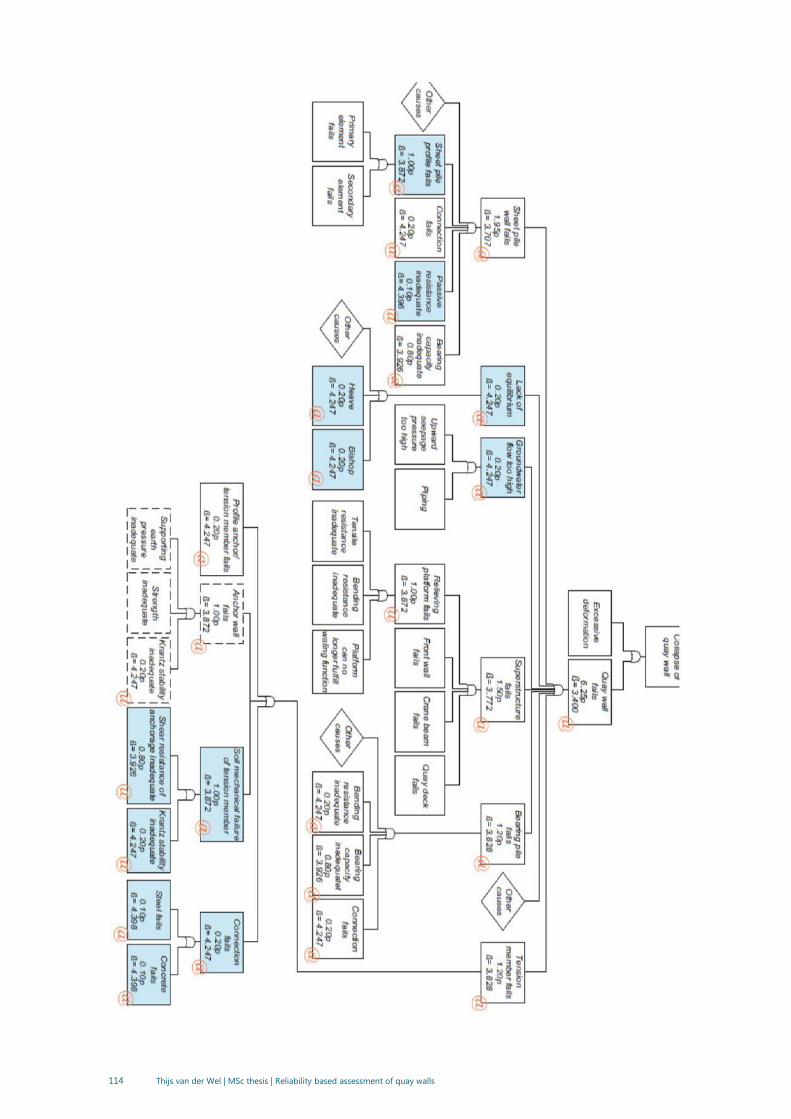
114 Thijs van der Wel | MSc thesis | Reliability based assessment of quay walls
115 Thijs van der Wel | MSc thesis | Reliability based assessment of quay walls
B
APPENDIX: PERFORMANCE OF ALGORITHMS OF OPENTURNS
In this appendix the working of the two available algorithms available in OpenTURNS is described together
with their performance when coupled with Plaxis.
COBYLA
COBYLA stands for Constrained Optimization By Linear Approximation and does not make use the calculation
of gradients. The exact working of this algorithm is quite difficult to understand and explain. According to
Powell (1994), COBYLA constructs linear polynomial approximations to the objective and constraint functions
by interpolation at the vertices of simplices (a simplex in n dimensions is the convex hull of n+1 points, n being
the number of variables). This number of random variables should be limited to approximately 9 because
otherwise the linear approximation can become highly inefficient. For further information reference is made
to (Powell, 1994).
The algorithm follows approximately the following steps.
1 The calculations are carried out in the standard space and starts with a calculation with median values for
all parameters.
2 After the mean value calculation, each individual parameter is varied by adding and subtracting 𝜌𝑏𝑒𝑔 ∗ 𝜎
to its mean value. The parameter 𝜌𝑏𝑒𝑔 should be provided by the user as input for the calculation.
3 After all parameters have been varied, the algorithm starts with searching to the design point.
4 After each iteration it is checked whether the convergence criteria are met. If this is the case the algorithm
is stopped and the output is showed in the interface of ProbAna.
Abdo-Rackwitz
The Abdo-Rackwitz algorithm is based on the definition of gradients. Also this method is carried out in the
standard space.
For every selected parameter the finite difference step (=step size) 𝜖 should be defined. This step size is used
to calculate the gradient of the limit state function with respect to a certain parameter. The gradient can be
calculated in two ways:
- Centered:
𝜕𝑍
𝜕𝑥𝑖=𝑍(𝑥 + 𝜖𝑖) − 𝑍(𝑥 − 𝜖𝑖)
2𝜖𝑖
- Non-centered: 𝜕𝑍
𝜕𝑥𝑖=𝑍(𝑥 + 𝜖𝑖) − 𝑍(𝑥)
𝜖𝑖
For a centered gradient the LSF has to be evaluated two times, whereas for the non-centered only one
evaluation is required. During every iteration the gradient is determined for every random variable, therefore
it is desirable with respect to computational time to use a non-centered gradient. On the other hand it is
known that the use of a centered gradient normally results in a more stable convergence.
For the step type a choice should be made between constant step size (the same step size for all iterations) or
a blended step size (only a constant step size during the first iteration). From tests with blended step type it
appeared that extremely unrealistic values are assigned to parameters (e.g. 90 degrees for the friction angle).
This can result in the calculation of situations which are not within the physical boundaries for which Plaxis is
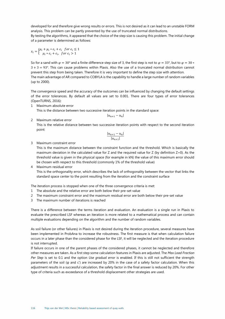
116 Thijs van der Wel | MSc thesis | Reliability based assessment of quay walls
developed for and therefore give wrong results or errors. This is not desired as it can lead to an unstable FORM
analysis. This problem can be partly prevented by the use of truncated normal distributions.
By testing the algorithms, it appeared that the choice of the step size is causing this problem. The initial change
of a parameter is determined as follows:
𝑥𝑖 = {𝜇𝑖 + 𝜇𝑖 ∗ 𝜖𝑖 + 𝜖𝑖 𝑓𝑜𝑟𝜖𝑖 ≤ 1𝜇𝑖 ∗ 𝜖𝑖 + 𝜖𝑖 ,𝑓𝑜𝑟𝜖𝑖 > 1
So for a sand with 𝜑 = 30° and a finite difference step size of 3, the first step is not to 𝜑 = 33°, but to 𝜑 = 30 ∗
3 + 3 = 93°. This can cause problems within Plaxis. Also the use of a truncated normal distribution cannot
prevent this step from being taken. Therefore it is very important to define the step size with attention.
The main advantage of AR compared to COBYLA is the capability to handle a large number of random variables
(up to 2000).
The convergence speed and the accuracy of the outcomes can be influenced by changing the default settings
of the error tolerances. By default all values are set to 0.001. There are four types of error tolerances
(OpenTURNS, 2016):
1 Maximum absolute error
This is the distance between two successive iteration points in the standard space:
|𝑢𝑛+1 − 𝑢𝑛|
2 Maximum relative error
This is the relative distance between two successive iteration points with respect to the second iteration
point: |𝑢𝑛+1 − 𝑢𝑛|
|𝑢𝑛+1|
3 Maximum constraint error
This is the maximum distance between the constraint function and the threshold. Which is basically the
maximum deviation in the calculated value for Z and the required value for Z (by definition Z=0). As the
threshold value is given in the physical space (for example in kN) the value of this maximum error should
be chosen with respect to this threshold (commonly 1% of the threshold value)
4 Maximum residual error
This is the orthogonality error, which describes the lack of orthogonality between the vector that links the
standard space center to the point resulting from the iteration and the constraint surface
The iteration process is stopped when one of the three convergence criteria is met:
1 The absolute and the relative error are both below their pre-set value
2 The maximum constraint error and the maximum residual error are both below their pre-set value
3 The maximum number of iterations is reached
There is a difference between the terms iteration and evaluation. An evaluation is a single run in Plaxis to
evaluate the prescribed LSF whereas an iteration is more related to a mathematical process and can contain
multiple evaluations depending on the algorithm and the number of random variables.
As soil failure (or other failures) in Plaxis is not desired during the iteration procedure, several measures have
been implemented in ProbAna to increase the robustness. The first measure is that when calculation failure
occurs in a later phase than the considered phase for the LSF, it will be neglected and the iteration procedure
is not interrupted.
If failure occurs in one of the parent phases of the considered phases, it cannot be neglected and therefore
other measures are taken. As a first step some calculation features in Plaxis are adjusted. The Max Load Fraction
Per Step is set to 0.1 and the option Use gradual error is enabled. If this is still not sufficient the strength
parameters of the soil (φ and c’) are increased by 20% in the case of a safety factor calculation. When this
adjustment results in a successful calculation, the safety factor in the final answer is reduced by 20%. For other
type of criteria such as exceedance of a threshold displacement other strategies are used.

117 Thijs van der Wel | MSc thesis | Reliability based assessment of quay walls
Comparison of both algorithms
First the results of a performance test by Rippi (2015) are elaborated, whereafter the results of additional tests
are described.
Rippi tested the performance of both algorithms on a Plaxis-model of an anchored sheet pile wall. The yield
stress (450 kPa) of the anchor was chosen as the limit in the limit state function of the anchor.
For the Cobyla algorithm three test were carried out with respectively 3, 10 and 19 parameters. When the
default values (0.001) of the error tolerances were used, no convergence was reached. Therefore it was required
to increase the error tolerances significantly to the values of Table B.1. It must be noted that in the research of
Rippi other convergence criteria are used than the ones in Probana. For convergence in the FORM analyses of
Rippi, all four error tolerances should be met, whereas in Probana, only a combination of certain errors
tolerances should be met.
Table B.1 Error tolerances COBYLA
Default value Adjusted value
Maximum absolute error 0.001 0.1
Maximum relative error 0.001 0.5
Maximum constraint error 0.001 0.2
Maximum residual error 0.001 0.1
Although convergence was reached with the adjusted values, the results of the calculation seemed incorrect
as a very high failure probability of around 0.35 was obtained. Also in all of the three cases the algorithm
stopped after 25 LSFE’s while the maximum number of LSFE was set to 100. This is strange because as shown
in Figure B.1, the maximum stress that was reached was around 375kPa which is significantly lower than the
yielding stress limit of 450 kPa.
Figure B.1 Iteration values for the anchor stress using 3 random variables. Source: Rippi (2015)
For the case of 19 random variables the algorithm performed even worse; the maximum stress in the anchor
did never surpass 267kPa. Also the algorithm was not able to variate its parameters properly. This is illustrated
in Figure B.2, which shows that the friction angle is kept constant during almost the entire optimization.
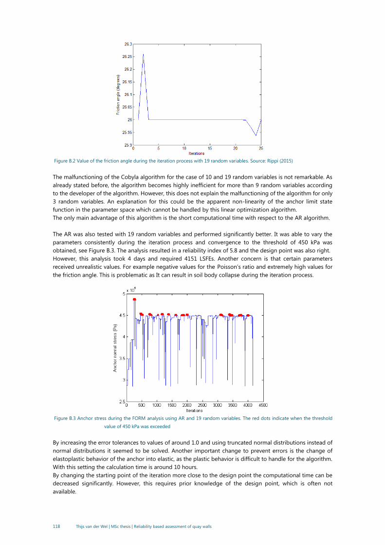
118 Thijs van der Wel | MSc thesis | Reliability based assessment of quay walls
Figure B.2 Value of the friction angle during the iteration process with 19 random variables. Source: Rippi (2015)
The malfunctioning of the Cobyla algorithm for the case of 10 and 19 random variables is not remarkable. As
already stated before, the algorithm becomes highly inefficient for more than 9 random variables according
to the developer of the algorithm. However, this does not explain the malfunctioning of the algorithm for only
3 random variables. An explanation for this could be the apparent non-linearity of the anchor limit state
function in the parameter space which cannot be handled by this linear optimization algorithm.
The only main advantage of this algorithm is the short computational time with respect to the AR algorithm.
The AR was also tested with 19 random variables and performed significantly better. It was able to vary the
parameters consistently during the iteration process and convergence to the threshold of 450 kPa was
obtained, see Figure B.3. The analysis resulted in a reliability index of 5.8 and the design point was also right.
However, this analysis took 4 days and required 4151 LSFEs. Another concern is that certain parameters
received unrealistic values. For example negative values for the Poisson’s ratio and extremely high values for
the friction angle. This is problematic as It can result in soil body collapse during the iteration process.
Figure B.3 Anchor stress during the FORM analysis using AR and 19 random variables. The red dots indicate when the threshold
value of 450 kPa was exceeded
By increasing the error tolerances to values of around 1.0 and using truncated normal distributions instead of
normal distributions it seemed to be solved. Another important change to prevent errors is the change of
elastoplastic behavior of the anchor into elastic, as the plastic behavior is difficult to handle for the algorithm.
With this setting the calculation time is around 10 hours.
By changing the starting point of the iteration more close to the design point the computational time can be
decreased significantly. However, this requires prior knowledge of the design point, which is often not
available.

119 Thijs van der Wel | MSc thesis | Reliability based assessment of quay walls
Due to the difference in convergence criteria between Rippi’s research and this one, extra tests were carried
out to get a better understanding of the algorithms and the influence of the tolerance errors on the
convergence of the FORM analysis. For this analysis the limit state function of the anchor of a combi-wall was
used. The threshold for the tensile strength in the anchor was set at the yield strength of 2993 kN.
First the performance of AR was tested. For the first run 6 parameters were selected as random variables.
The convergence criteria settings were the following:
Table B.2 Convergence criteria
Value
Maximum absolute error 0.05
Maximum relative error 0.05
Maximum constraint error 25 kN
Maximum residual error 0.05
Gradient type Non-centered
Step type Blended
Max. Iterations 50
With this settings convergence was reached after 27 iterations (273 LSFE’s) which took 10 hours. All parameter
distributions were chosen as Truncated normal to prevent physically unrealistic values. The obtained reliability
index was 4.03 and also the design point seemed correct. When considering the development of the
convergence error (Figure B.4), it can be concluded that the constraint error is already below its limit (25 kN)
after two iterations.
Figure B.4 Convergence errors
The three other errors required more iterations (Figure B.5). The algorithm was stopped because both the
constraint and the residual error requirements were met.
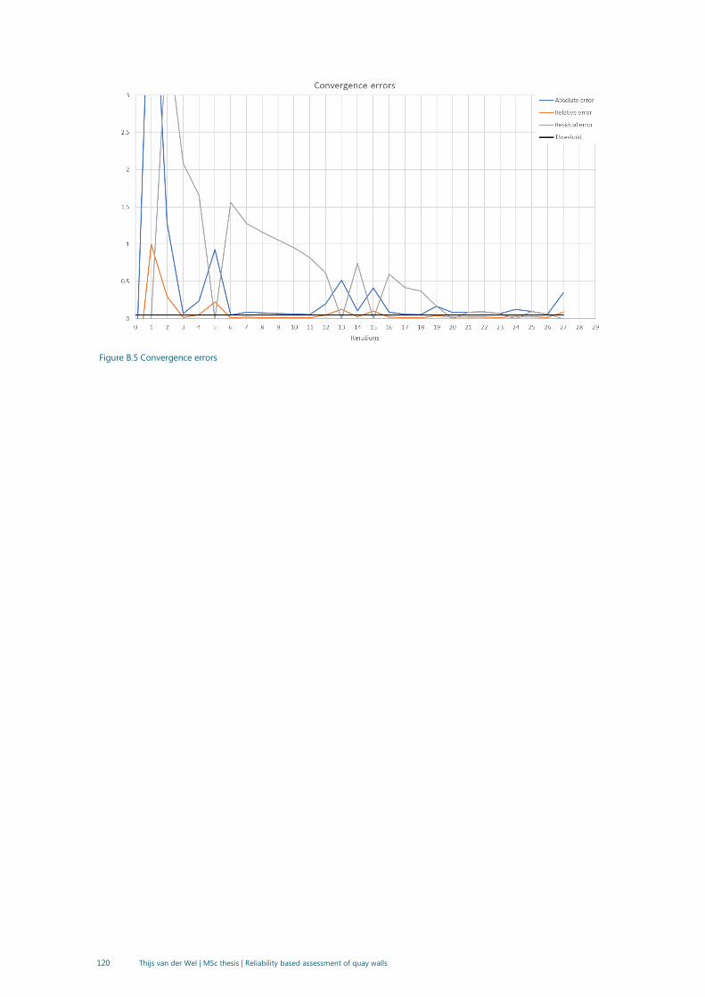
120 Thijs van der Wel | MSc thesis | Reliability based assessment of quay walls
Figure B.5 Convergence errors
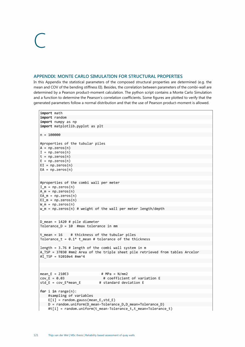
121 Thijs van der Wel | MSc thesis | Reliability based assessment of quay walls
C
APPENDIX: MONTE CARLO SIMULATION FOR STRUCTURAL PROPERTIES
In this Appendix the statistical parameters of the composed structural properties are determined (e.g. the
mean and COV of the bending stiffness EI). Besides, the correlation between parameters of the combi-wall are
determined by a Pearson product-moment calculation. The python script contains a Monte Carlo Simulation
and a function to determine the Pearson’s correlation coefficients. Some figures are plotted to verify that the
generated parameters follow a normal distribution and that the use of Pearson product-moment is allowed.
import math import random import numpy as np import matplotlib.pyplot as plt n = 100000 #properties of the tubular piles A = np.zeros(n) I = np.zeros(n) t = np.zeros(n) E = np.zeros(n) EI = np.zeros(n) EA = np.zeros(n) #properties of the combi wall per meter I_m = np.zeros(n) A_m = np.zeros(n) EA_m = np.zeros(n) EI_m = np.zeros(n) W_m = np.zeros(n) w_m = np.zeros(n) # weight of the wall per meter length/depth D_mean = 1420 # pile diameter Tolerance_D = 10 #max tolerance in mm t_mean = 16 # thickness of the tubular piles Tolerance_t = 0.1* t_mean # tolerance of the thickness length = 3.76 # length of the combi wall system in m A_TSP = 37030 #mm2 Area of the triple sheet pile retrieved from tables Arcelor #I_TSP = 92010e4 #mm^4 mean_E = 210E3 # MPa = N/mm2 cov_E = 0.03 # coefficient of variation E std_E = cov_E*mean_E # standard deviation E for i in range(n): #sampling of variables E[i] = random.gauss(mean_E,std_E) D = random.uniform(D_mean-Tolerance_D,D_mean+Tolerance_D) #t[i] = random.uniform(t_mean-Tolerance_t,t_mean+Tolerance_t)
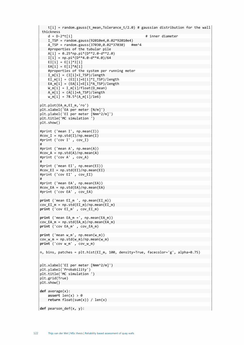
122 Thijs van der Wel | MSc thesis | Reliability based assessment of quay walls
t[i] = random.gauss(t_mean,Tolerance_t/2.0) # gaussian distribution for the wall thickness d = D-2*t[i] # inner diameter I_TSP = random.gauss(92010e4,0.02*92010e4) A_TSP = random.gauss(37030,0.02*37030) #mm^4 #properties of the tubular pile A[i] = 0.25*np.pi*(D**2.0-d**2.0) I[i] = np.pi*(D**4.0-d**4.0)/64 EI[i] = E[i]*I[i] EA[i] = E[i]*A[i] #properties of the system per running meter I_m[i] = (I[i]+I_TSP)/length EI_m[i] = (EI[i]+E[i]*I_TSP)/length EA_m[i] = (EA[i]+E[i]*A_TSP)/length W_m[i] = I_m[i]/float(D_mean) A_m[i] = (A[i]+A_TSP)/length w_m[i] = 78.5*(A_m[i]/1e6) plt.plot(EA_m,EI_m,'ro') plt.xlabel('EA per meter [N/m]') plt.ylabel('EI per meter [Nmm^2/m]') plt.title('MC simulation ') plt.show() #print ('mean I', np.mean(I)) #cov_I = np.std(I)/np.mean(I) #print ('cov I' , cov_I) # #print ('mean A', np.mean(A)) #cov_A = np.std(A)/np.mean(A) #print ('cov A' , cov_A) # #print ('mean EI', np.mean(EI)) #cov_EI = np.std(EI)/np.mean(EI) #print ('cov EI' , cov_EI) # #print ('mean EA', np.mean(EA)) #cov_EA = np.std(EA)/np.mean(EA) #print ('cov EA' , cov_EA) print ('mean EI_m ', np.mean(EI_m)) cov_EI_m = np.std(EI_m)/np.mean(EI_m) print ('cov EI_m' , cov_EI_m) print ('mean EA_m =', np.mean(EA_m)) cov_EA_m = np.std(EA_m)/np.mean(EA_m) print ('cov EA_m' , cov_EA_m) print ('mean w_m', np.mean(w_m)) cov_w_m = np.std(w_m)/np.mean(w_m) print ('cov w_m' , cov_w_m) n, bins, patches = plt.hist(EI_m, 100, density=True, facecolor='g', alpha=0.75) plt.xlabel('EI per meter [Nmm^2/m]') plt.ylabel('Probability') plt.title('MC simulation ') plt.grid(True) plt.show() def average(x): assert len(x) > 0 return float(sum(x)) / len(x) def pearson_def(x, y):

123 Thijs van der Wel | MSc thesis | Reliability based assessment of quay walls
assert len(x) == len(y) n = len(x) assert n > 0 avg_x = average(x) avg_y = average(y) diffprod = 0 xdiff2 = 0 ydiff2 = 0 for idx in range(n): xdiff = x[idx] - avg_x ydiff = y[idx] - avg_y diffprod += xdiff * ydiff xdiff2 += xdiff * xdiff ydiff2 += ydiff * ydiff return diffprod / math.sqrt(xdiff2 * ydiff2) print ('p_EAm_wm = ',pearson_def(EA_m,w_m) ) print ('p_EAm_Am = ',pearson_def(EA_m,A_m) ) print ('p_Wm_wm = ',pearson_def(W_m,w_m) ) print ('p_Wm_Am = ',pearson_def(W_m,A_m) )

124 Thijs van der Wel | MSc thesis | Reliability based assessment of quay walls
D
APPENDIX: FAULT TREE SIMPLE QUAY WALL
Below is the fault tree of CUR211 (2005)given, in which the failure space distributed is applied.
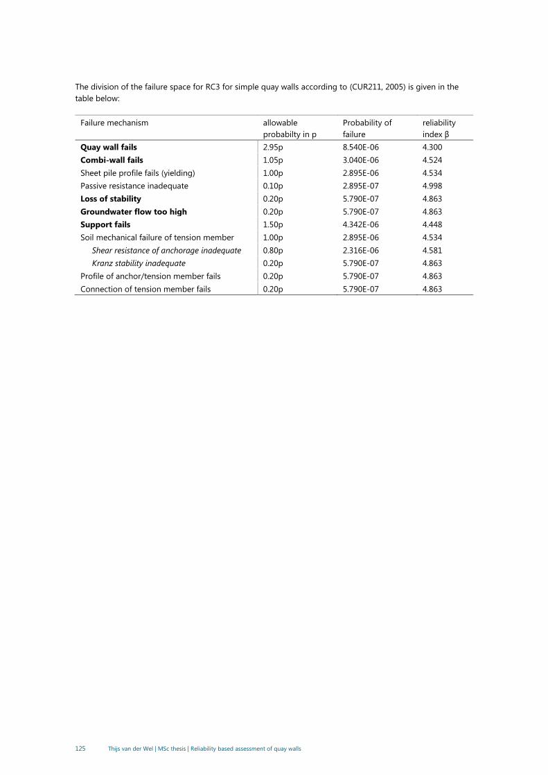
125 Thijs van der Wel | MSc thesis | Reliability based assessment of quay walls
The division of the failure space for RC3 for simple quay walls according to (CUR211, 2005) is given in the
table below:
Failure mechanism allowable
probabilty in p
Probability of
failure
reliability
index β
Quay wall fails 2.95p 8.540E-06 4.300
Combi-wall fails 1.05p 3.040E-06 4.524
Sheet pile profile fails (yielding) 1.00p 2.895E-06 4.534
Passive resistance inadequate 0.10p 2.895E-07 4.998
Loss of stability 0.20p 5.790E-07 4.863
Groundwater flow too high 0.20p 5.790E-07 4.863
Support fails 1.50p 4.342E-06 4.448
Soil mechanical failure of tension member 1.00p 2.895E-06 4.534
Shear resistance of anchorage inadequate 0.80p 2.316E-06 4.581
Kranz stability inadequate 0.20p 5.790E-07 4.863
Profile of anchor/tension member fails 0.20p 5.790E-07 4.863
Connection of tension member fails 0.20p 5.790E-07 4.863

126 Thijs van der Wel | MSc thesis | Reliability based assessment of quay walls
E
APPENDIX: PLAXIS OUTPUT RESULTS LBBR
In this appendix, the Plaxis output results in the design point of FORM is shown.
LS1: Yielding of the wall
Output results for LSF: 𝑍 = 4045 −𝑀𝑆
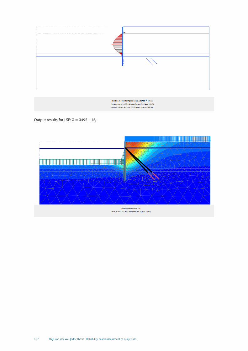
127 Thijs van der Wel | MSc thesis | Reliability based assessment of quay walls
Output results for LSF: 𝑍 = 3495 −𝑀𝑆
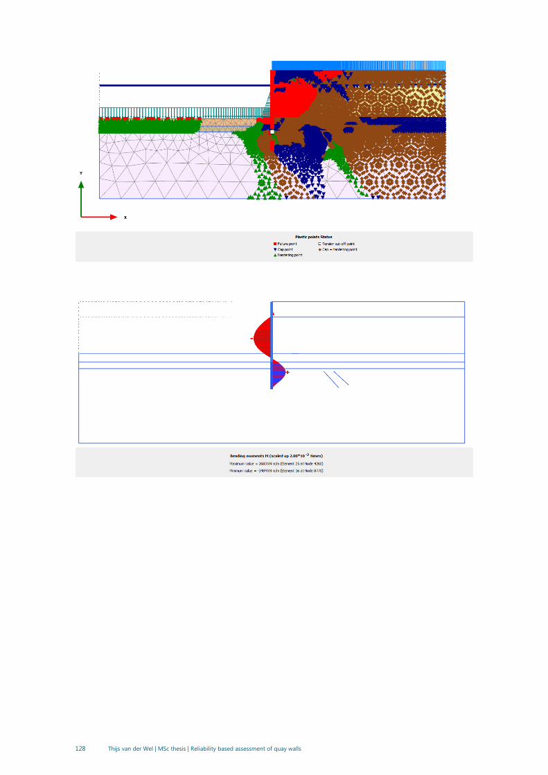
128 Thijs van der Wel | MSc thesis | Reliability based assessment of quay walls
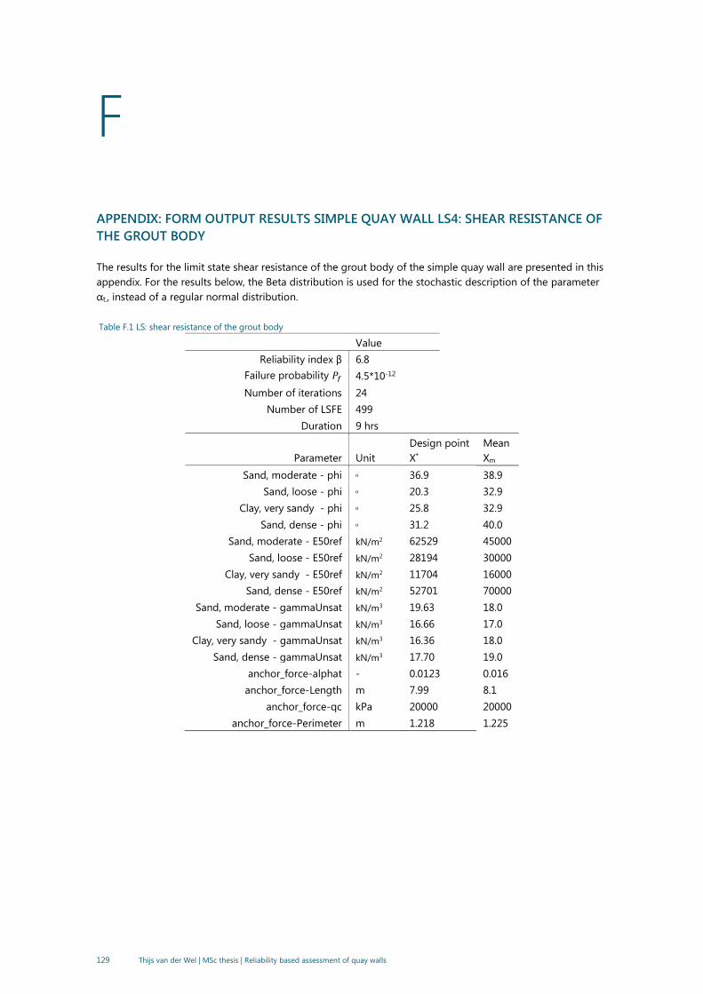
129 Thijs van der Wel | MSc thesis | Reliability based assessment of quay walls
F
APPENDIX: FORM OUTPUT RESULTS SIMPLE QUAY WALL LS4: SHEAR RESISTANCE OF
THE GROUT BODY
The results for the limit state shear resistance of the grout body of the simple quay wall are presented in this
appendix. For the results below, the Beta distribution is used for the stochastic description of the parameter
αt., instead of a regular normal distribution.
Table F.1 LS: shear resistance of the grout body
Value
Reliability index β 6.8
Failure probability 𝑃𝑓 4.5*10-12
Number of iterations 24
Number of LSFE 499
Duration 9 hrs
Parameter
Unit
Design point
X*
Mean
Xm
Sand, moderate - phi ᵒ 36.9 38.9
Sand, loose - phi ᵒ 20.3 32.9
Clay, very sandy - phi ᵒ 25.8 32.9
Sand, dense - phi ᵒ 31.2 40.0
Sand, moderate - E50ref kN/m2 62529 45000
Sand, loose - E50ref kN/m2 28194 30000
Clay, very sandy - E50ref kN/m2 11704 16000
Sand, dense - E50ref kN/m2 52701 70000
Sand, moderate - gammaUnsat kN/m3 19.63 18.0
Sand, loose - gammaUnsat kN/m3 16.66 17.0
Clay, very sandy - gammaUnsat kN/m3 16.36 18.0
Sand, dense - gammaUnsat kN/m3 17.70 19.0
anchor_force-alphat - 0.0123 0.016
anchor_force-Length m 7.99 8.1
anchor_force-qc kPa 20000 20000
anchor_force-Perimeter m 1.218 1.225

130 Thijs van der Wel | MSc thesis | Reliability based assessment of quay walls

131 Thijs van der Wel | MSc thesis | Reliability based assessment of quay walls
G
APPENDIX: CALCULATIONS RESULTS FORM FOR DERIVING PARTIAL FACTORS SIMPLE
QUAY WALL
The results of the limit state evaluations for the derivation of partial factors are given below.
Table G.1 LS1: Yielding of the wall
FORM event probability 4.9674E-09
General reliability index 5.732
Hasofer reliability index 5.732
Number of evaluations 103
Number of iterations 5
The standard point origin is in the
failure space
FALSE
Parameter Standard space
design point
Physical space
design point
Importance
factors U-space
Importance
factors Y-space
ZandSchoonMatig-E50ref 0.221 47771.61 0.001 0.001
ZandSchoonLos-E50ref -1.061 22052.32 0.034 0.033
KleiSterkZandig-E50ref -0.837 12547.40 0.021 0.020
ZandSchoonVast-E50ref -0.437 61650.54 0.006 0.006
ZandSchoonMatig-phi 0.697 41.74 0.015 0.016
ZandSchoonLos-phi -3.283 21.70 0.328 0.345
KleiSterkZandig-phi -1.161 28.51 0.041 0.052
ZandSchoonVast-phi 0.107 39.98 0.000 0.000
ZandSchoonMatig-gammaUnsat 0.722 18.85 0.016 0.026
ZandSchoonLos-gammaUnsat 1.444 16.42 0.063 0.014
KleiSterkZandig-gammaUnsat -0.350 16.97 0.004 0.038
ZandSchoonVast-gammaUnsat -0.022 18.82 0.000 0.001
Surcharge-qy_start -1.129 -44.51 0.039 0.037
Combiwall_redesign-t_tube -1.136 0.02 0.039 0.038
Combiwall_redesign-d_tube -0.224 1.42 0.002 0.001
max_stress_plate_plus_sign-
fy_tube
-3.580 411497.07 0.390 0.373
Final absolute error 1.35
Final relative error 0.23
Final residual error 3.1032E-17
Final constraint error 3456.7

132 Thijs van der Wel | MSc thesis | Reliability based assessment of quay walls
Table G.2 LS2: Yielding of the anchor bar
FORM event probability 7.55E-08
General reliability index 5.25
Hasofer reliability index 5.25
Number of evaluations 147
Number of iterations 7
The standard point origin is in
the failure space
FALSE
Parameter Standard space
design point
Physical space
design point
Importance
factors U-space
Importance
factors Y-space
ZandSchoonMatig-E50ref 0.654 54152.8 0.015 0.015
ZandSchoonLos-E50ref -0.588 25296.5 0.013 0.012
KleiSterkZandig-E50ref -0.439 14083.9 0.007 0.007
ZandSchoonVast-E50ref 0.156 73226.2 0.001 0.001
ZandSchoonMatig-phi -0.418 38.0 0.006 0.002
ZandSchoonLos-phi -2.884 23.3 0.302 0.306
KleiSterkZandig-phi -0.791 30.0 0.023 0.027
ZandSchoonVast-phi -0.291 39.0 0.003 0.002
ZandSchoonMatig-
gammaUnsat
0.943 18.8 0.032 0.028
ZandSchoonLos-gammaUnsat 0.820 16.3 0.024 0.021
KleiSterkZandig-gammaUnsat -0.233 17.4 0.002 0.018
ZandSchoonVast-
gammaUnsat
-0.017 19.0 0.000 0.000
Borehole_1-Head 0.038 -0.8 0.000 0.000
Surcharge-qy_start -0.830 -43.3 0.025 0.024
anchor_force-fy -3.781 417205 0.518 0.507
anchor_force-A -0.886 0.005 0.028 0.028
Final absolute error 0.758
Final relative error 0.144
Final residual error 0.000
Final constraint error 7.737
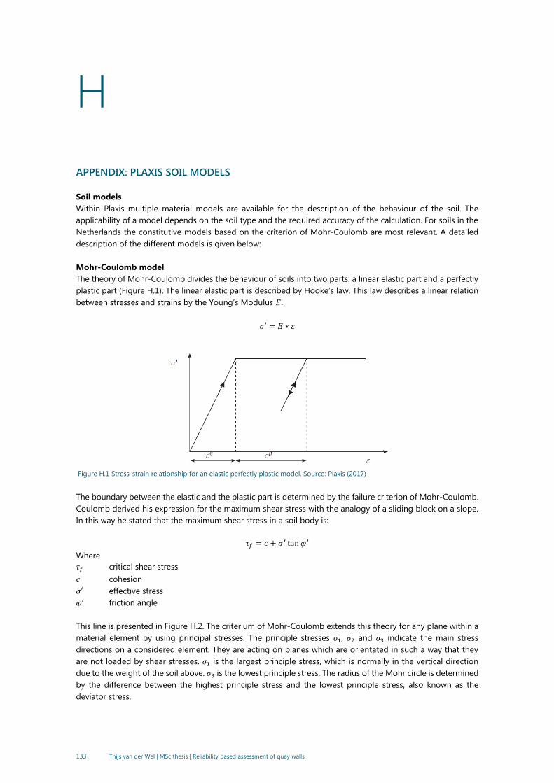
133 Thijs van der Wel | MSc thesis | Reliability based assessment of quay walls
H
APPENDIX: PLAXIS SOIL MODELS
Soil models
Within Plaxis multiple material models are available for the description of the behaviour of the soil. The
applicability of a model depends on the soil type and the required accuracy of the calculation. For soils in the
Netherlands the constitutive models based on the criterion of Mohr-Coulomb are most relevant. A detailed
description of the different models is given below:
Mohr-Coulomb model
The theory of Mohr-Coulomb divides the behaviour of soils into two parts: a linear elastic part and a perfectly
plastic part (Figure H.1). The linear elastic part is described by Hooke’s law. This law describes a linear relation
between stresses and strains by the Young’s Modulus 𝐸.
𝜎′ = 𝐸 ∗ 휀
Figure H.1 Stress-strain relationship for an elastic perfectly plastic model. Source: Plaxis (2017)
The boundary between the elastic and the plastic part is determined by the failure criterion of Mohr-Coulomb.
Coulomb derived his expression for the maximum shear stress with the analogy of a sliding block on a slope.
In this way he stated that the maximum shear stress in a soil body is:
𝜏𝑓 = 𝑐 + 𝜎′ tan 𝜑′
Where
𝜏𝑓 critical shear stress
𝑐 cohesion
𝜎′ effective stress
𝜑′ friction angle
This line is presented in Figure H.2. The criterium of Mohr-Coulomb extends this theory for any plane within a
material element by using principal stresses. The principle stresses 𝜎1, 𝜎2 and 𝜎3 indicate the main stress
directions on a considered element. They are acting on planes which are orientated in such a way that they
are not loaded by shear stresses. 𝜎1 is the largest principle stress, which is normally in the vertical direction
due to the weight of the soil above. 𝜎3 is the lowest principle stress. The radius of the Mohr circle is determined
by the difference between the highest principle stress and the lowest principle stress, also known as the
deviator stress.
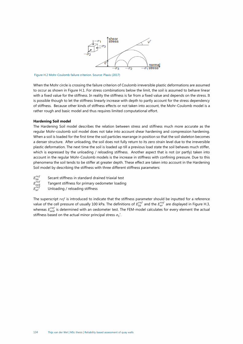
134 Thijs van der Wel | MSc thesis | Reliability based assessment of quay walls
Figure H.2 Mohr-Coulomb failure criterion. Source: Plaxis (2017)
When the Mohr circle is crossing the failure criterion of Coulomb irreversible plastic deformations are assumed
to occur as shown in Figure H.1. For stress combinations below the limit, the soil is assumed to behave linear
with a fixed value for the stiffness. In reality the stiffness is far from a fixed value and depends on the stress. It
is possible though to let the stiffness linearly increase with depth to partly account for the stress dependency
of stiffness. Because other kinds of stiffness effects or not taken into account, the Mohr-Coulomb model is a
rather rough and basic model and thus requires limited computational effort.
Hardening Soil model
The Hardening Soil model describes the relation between stress and stiffness much more accurate as the
regular Mohr-coulomb soil model does not take into account shear hardening and compression hardening.
When a soil is loaded for the first time the soil particles rearrange in position so that the soil skeleton becomes
a denser structure. After unloading, the soil does not fully return to its zero strain level due to the irreversible
plastic deformation. The next time the soil is loaded up till a previous load state the soil behaves much stiffer,
which is expressed by the unloading / reloading stiffness. Another aspect that is not (or partly) taken into
account in the regular Mohr-Coulomb models is the increase in stiffness with confining pressure. Due to this
phenomena the soil tends to be stiffer at greater depth. These effect are taken into account in the Hardening
Soil model by describing the stiffness with three different stiffness parameters:
𝐸50𝑟𝑒𝑓
Secant stiffness in standard drained triaxial test
𝐸𝑜𝑒𝑑𝑟𝑒𝑓
Tangent stiffness for primary oedometer loading
𝐸𝑢𝑟𝑟𝑒𝑓
Unloading / reloading stiffness
The superscript 𝑟𝑒𝑓 is introduced to indicate that the stiffness parameter should be inputted for a reference
value of the cell pressure of usually 100 kPa. The definitions of 𝐸50𝑟𝑒𝑓
and the 𝐸𝑢𝑟𝑟𝑒𝑓
are displayed in Figure H.3,
whereas 𝐸𝑜𝑒𝑑𝑟𝑒𝑓
is determined with an oedometer test. The FEM-model calculates for every element the actual
stiffness based on the actual minor principal stress 𝜎3′.
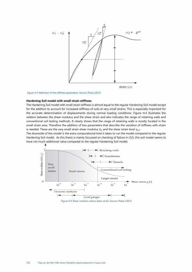
135 Thijs van der Wel | MSc thesis | Reliability based assessment of quay walls
Figure H.3 Definition of the stiffness parameters. Source: Plaxis (2017)
Hardening Soil model with small strain stiffness
The Hardening Soil model with small strain stiffness is almost equal to the regular Hardening Soil model except
for the addition to account for increased stiffness of soils at very small strains. This is especially important for
the accurate determination of displacements during normal loading conditions. Figure H.4 illustrates the
relation between the shear modulus and the shear strain and also indicates the range of retaining walls and
conventional soil testing methods. It clearly shows that the range of retaining walls is mostly located in the
small strain area. Therefore the addition of two parameters that describe the variation of stiffness with strain
is needed. These are the very small strain shear modulus 𝐺0 and the shear strain level 𝛾0.7.
The downside of this model is the extra computational time it takes to run the model compared to the regular
Hardening Soil model. As this thesis is mainly focussed on checking of failure in ULS, this soil model seems to
have not much additional value compared to the regular Hardening Soil model.
Figure H.4 Shear modulus versus shear strain. Source: Plaxis (2017)
136 Thijs van der Wel | MSc thesis | Reliability based assessment of quay walls
I
APPENDIX: LONGITUDINAL SOIL PROFILE AND USED CPT
On the next page, the longitudinal soil profile for the EMO quay wall is shown. The black square indicates the
location of the closest nearby CPT with respect to the measurement pit that is used in this research.
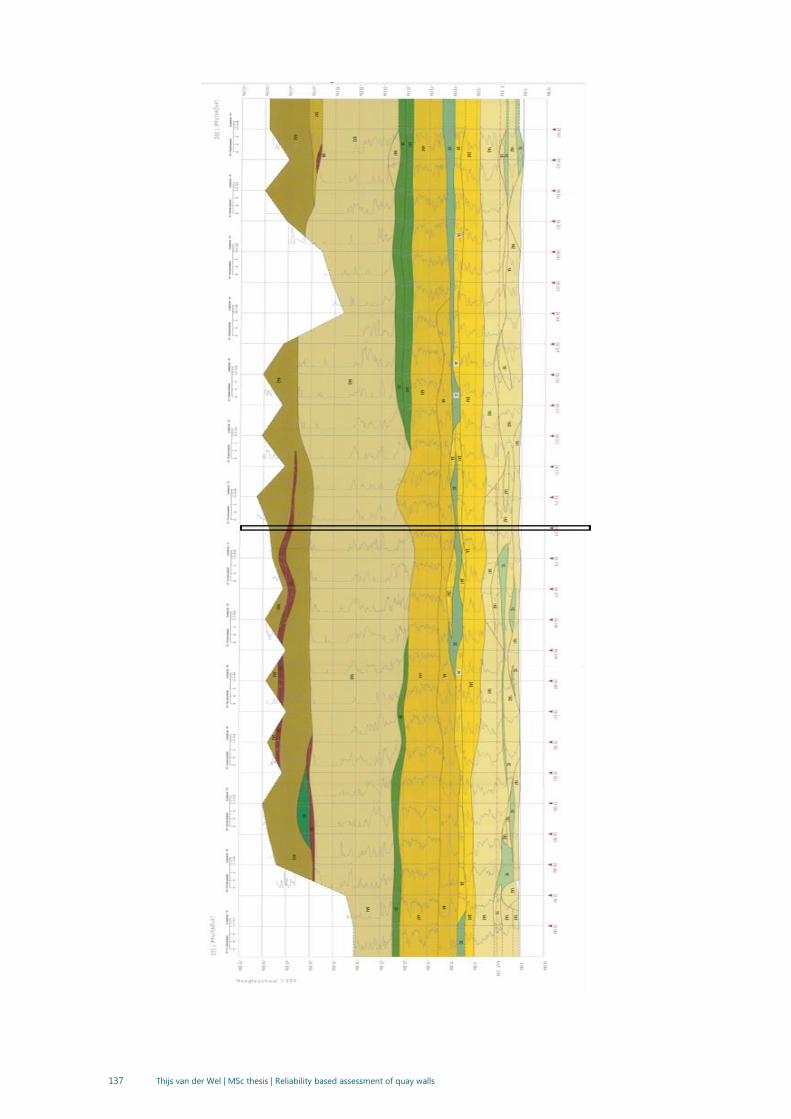
137 Thijs van der Wel | MSc thesis | Reliability based assessment of quay walls

138 Thijs van der Wel | MSc thesis | Reliability based assessment of quay walls

139 Thijs van der Wel | MSc thesis | Reliability based assessment of quay walls

140 Thijs van der Wel | MSc thesis | Reliability based assessment of quay walls
J
APPENDIX: CALCULATION RESULTS EMO
The results of the sensitivity analysis with uncorrelated parameters for the limit state yielding of the combi-
wall are given below.
FORM event probability 0.00014
General reliability index 3.62
Hasofer reliability index 3.62
Number of evaluations 141
Number of iterations 5
The standard point origin is in
the failure space
FALSE
Parameter Standard space
design point
Physical space
design point
Importance
factors
U-space
Importance
factors
Y-space
SandModerate1A2-phi -0.14 34.52 0.00 0.00
SandDense2A3-phi -0.18 36.84 0.00 0.00
ClayWSandyModerate2C-phi -0.08 24.81 0.00 0.00
Sand4A-phi -0.23 34.21 0.00 0.00
SandClayLayers4A1-phi -1.02 26.76 0.08 0.08
SandDense5A3-phi -3.27 25.24 0.81 0.81
SandModerate1A2-E50ref 0.08 48193 0.00 0.00
SandDense2A3-E50ref -0.26 43455 0.01 0.01
ClayWSandyModerate2C-
E50ref
-0.03 3068 0.00 0.00
Sand4A-E50ref -0.11 43517 0.00 0.00
SandClayLayers4A1-E50ref -0.05 40412 0.00 0.00
SandDense5A3-E50ref -0.08 45889 0.00 0.00
SandModerate1A2-
gammaUnsat
0.27 18.24 0.01 0.01
SandDense2A3-gammaUnsat 0.15 19.14 0.00 0.00
ClayWSandyModerate2C-
gammaUnsat
0.02 17.02 0.00 0.00
Sand4A-gammaUnsat 0.06 19.06 0.00 0.00
SandClayLayers4A1-
gammaUnsat
0.00 18.00 0.00 0.00
SandDense5A3-gammaUnsat -0.83 18.21 0.05 0.05
CombiWall-t_tube -0.11 0.02 0.00 0.00

141 Thijs van der Wel | MSc thesis | Reliability based assessment of quay walls
CombiWall-d_tube 0.01 1.42 0.00 0.00
fy_tube -0.63 480653 0.03 0.03
Final absolute error 1.220
Final relative error 0.337
Final residual error 4.66E-17
Final constraint error 2240.22
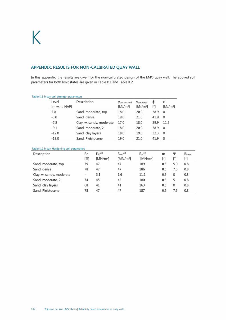
142 Thijs van der Wel | MSc thesis | Reliability based assessment of quay walls
K
APPENDIX: RESULTS FOR NON-CALIBRATED QUAY WALL
In this appendix, the results are given for the non-calibrated design of the EMO quay wall. The applied soil
parameters for both limit states are given in Table K.1 and Table K.2.
Table K.1 Mean soil strength parameters
Level
[m w.r.t. NAP]
Description γunsaturated
[kN/m3]
γsaturated
[kN/m3]
ϕ’
[°]
c’
[kN/m2]
5.0 Sand, moderate, top 18.0 20.0 38.9 0
-3.0 Sand, dense 19.0 21.0 41.9 0
-7.8 Clay, w. sandy, moderate 17.0 18.0 29.9 11.2
-9.1 Sand, moderate, 2 18.0 20.0 38.9 0
-12.0 Sand, clay layers 18.0 19.0 32.3 0
-19.0 Sand, Pleistocene 19.0 21.0 41.9 0
Table K.2 Mean Hardening soil parameters
Description Re
[%]
E50ref
[MN/m2]
Eoedref
[MN/m2]
Eurref
[MN/m2]
m
[-]
Ψ
[°]
Rinter
[-]
Sand, moderate, top 79 47 47 189 0.5 5.0 0.8
Sand, dense 78 47 47 186 0.5 7.5 0.8
Clay, w. sandy, moderate - 3.1 1,6 11,1 0.9 0 0.8
Sand, moderate, 2 74 45 45 180 0.5 5 0.8
Sand, clay layers 68 41 41 163 0.5 0 0.8
Sand, Pleistocene 78 47 47 187 0.5 7.5 0.8

143 Thijs van der Wel | MSc thesis | Reliability based assessment of quay walls
Table K.3 Results for the limit state soil mechanical failure
FORM event probability 2.36E-05
General reliability index 4.069238704
Hasofer reliability index 4.069238704
Number of evaluations 22
Number of iterations 2
The standard point origin is in
the failure space
FALSE
Parameter Standard space
design point
Physical space
design point
Importance
factors U-space
Importance
factors Y-space
SandModeratetop-phi -0.24 37.95 0.00 0.00
SandDense-phi -0.20 40.95 0.00 0.00
ClayWSandyModerate-phi 0.00 29.90 0.00 0.00
Sand, moderate, 2 -phi -0.19 38.16 0.00 0.00
SandClayLayers-phi -0.53 30.59 0.02 0.01
Sand, Pleistocene - phi -3.95 25.32 0.94 0.63
Sand, Pleistocene -
gammaUnsat
-0.74 16.52 0.03 0.28
Sand, Pleistocene - E50ref -0.03 31521 0.00 0.07
Final absolute error 0.238
Final relative error 0.058
Final residual error 1.52E-18
Final constraint error 0.000893351
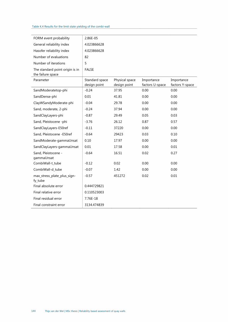
144 Thijs van der Wel | MSc thesis | Reliability based assessment of quay walls
Table K.4 Results for the limit state yielding of the combi-wall
FORM event probability 2.86E-05
General reliability index 4.023866628
Hasofer reliability index 4.023866628
Number of evaluations 82
Number of iterations 5
The standard point origin is in
the failure space
FALSE
Parameter Standard space
design point
Physical space
design point
Importance
factors U-space
Importance
factors Y-space
SandModeratetop-phi -0.24 37.95 0.00 0.00
SandDense-phi 0.01 41.81 0.00 0.00
ClayWSandyModerate-phi -0.04 29.78 0.00 0.00
Sand, moderate, 2-phi -0.24 37.94 0.00 0.00
SandClayLayers-phi -0.87 29.49 0.05 0.03
Sand, Pleistocene -phi -3.76 26.12 0.87 0.57
SandClayLayers-E50ref -0.11 37220 0.00 0.00
Sand, Pleistocene -E50ref -0.64 29423 0.03 0.10
SandModerate-gammaUnsat 0.10 17.97 0.00 0.00
SandClayLayers-gammaUnsat 0.01 17.58 0.00 0.01
Sand, Pleistocene -
gammaUnsat
-0.64 16.51 0.02 0.27
CombiWall-t_tube -0.12 0.02 0.00 0.00
CombiWall-d_tube -0.07 1.42 0.00 0.00
max_stress_plate_plus_sign-
fy_tube
-0.57 451272 0.02 0.01
Final absolute error 0.444729821
Final relative error 0.110523003
Final residual error 7.76E-18
Final constraint error 3134.474839
