Uncertainty quantification of an Aviation Environmental Toolsuite

Douglas Allaire a, George Noel b, Karen Willcox a,n, Rebecca Cointin c

a Department of Aeronautics and Astronautics, Massachusetts Institute of Technology, Cambridge, MA 02139, United Statesb Volpe National Transportation Systems Center, Cambridge, MA 02142, United Statesc Office of the Environment and Energy, FAA, Washington, DC, United States

a r t i c l e i n f o

Article history:Received 14 March 2013Received in revised form21 October 2013Accepted 1 January 2014Available online 15 January 2014

Keywords:Uncertainty quantificationSensitivity analysisEnvironmental system modelsAircraft emissions model

a b s t r a c t

This paper describes uncertainty quantification (UQ) of a complex system computational tool thatsupports policy-making for aviation environmental impact. The paper presents the methods needed tocreate a tool that is “UQ-enabled” with a particular focus on how to manage the complexity of long runtimes and massive input/output datasets. These methods include a process to quantify parameteruncertainties via data, documentation and expert opinion, creating certified surrogate models toaccelerate run-times while maintaining confidence in results, and executing a range of mathematicalUQ techniques such as uncertainty propagation and global sensitivity analysis. The results and discussionaddress aircraft performance, aircraft noise, and aircraft emissions modeling.

& 2014 Elsevier Ltd. All rights reserved.

1. Introduction

Uncertainty quantification (UQ) broadly entails quantitativecharacterization, management, and reduction of uncertainty inapplications, and encompasses many different elements (e.g.,uncertainty analysis, sensitivity analysis, optimization underuncertainty, design validation, and model calibration). UQ isbecoming an essential aspect of the development and use ofcomputational simulation and modeling tools. For example, theNational Academy of Sciences has recognized the “ubiquity ofuncertainty in computational estimates of reality and the necessityfor its quantification” [28] while NASA established a formalstandard setting requirements and recommendations for uncer-tainty assessment in the use of modeling and simulation tosupport critical decisions [27]. This paper describes how state-of-the-art UQ methods together with surrogate models are combinedto achieve UQ of a real-world complex system modeling tool thatsupports policy-making for aviation environmental impact.

The FAA Office of Environment and Energy, in collaborationwith Transport Canada and NASA, is developing a suite ofcomputational tools to support decision and policy-making foraviation environmental impact. This Environmental Toolsuiteincludes integrated models of airline economics, environmentaleconomics, aircraft operations, aircraft performance, aircraft emis-sions, noise, local air quality, and global climate. The main goal ofthe effort is to develop a new critically needed capability to

characterize and quantify the interdependencies among aviation-related noise and emissions, impacts on health and welfare, andindustry and consumer costs, under different policy, technology,operational, and market scenarios. A comprehensive UQ effort isan important component of this tool development, with the follow-ing specific goals: (1) provide sensitivity analyses of the outputs touncertainties in the inputs and assumptions, establishing proceduresfor future assessment efforts; (2) identify gaps in functionality withinthe tools, leading to the identification of high-priority areas forfurther development; (3) assess confidence in the evaluation ofvarious analysis scenarios such as oxides of nitrogen (NOx) stringencyand future aircraft technologies; and (4) continue to contribute to thedevelopment of external understanding of the FAA Toolsuite cap-abilities. A critical aspect of a comprehensive UQ effort is the ability tomake the behavior of a tool both transparent and comprehensible todecision makers while incorporating a variety of uncertainties in thetool. To ensure this, the overall UQ process for the EnvironmentalToolsuite includes tasks related to expert review, verification, valida-tion, capability demonstration, and parametric uncertainty/sensitivityanalysis [17]. We focus here on the UQ challenges related to enablingparametric uncertainty and sensitivity analyses.

The scale and complexity of the problem make UQ for thistoolset a daunting task that challenges state-of-the-art in UQmethods. Many of the component computational models havelong run times. There is a large amount of data even for a singledeterministic analysis (e.g., an analysis of one year involves overtwo million flight operations with 350 aircraft types). Several ofthe component computational models are built on legacy toolsthat were designed with a firmly deterministic mindset; thus,there are few opportunities for intrusive UQ methods. And while

Contents lists available at ScienceDirect

journal homepage: www.elsevier.com/locate/ress

Reliability Engineering and System Safety

0951-8320/$ - see front matter & 2014 Elsevier Ltd. All rights reserved.http://dx.doi.org/10.1016/j.ress.2014.01.002

n Corresponding author.E-mail address: kwillcox@mit.edu (K. Willcox).

Reliability Engineering and System Safety 126 (2014) 14–24

there is a recognition of a need to quantify and account foruncertainties, formal characterizations of parameter uncertainties(e.g., via probabilistic distributions) are not typically available forany of the component models.

In this paper, we present methodology and results for UQ of theAviation Environmental Design Tool (AEDT), one component of theoverall Environmental Toolsuite, but in itself a complex systemmodel embodying all of these challenges. Section 2 providesbackground on AEDT and its constituent models. Section 3describes the methods developed to achieve UQ of AEDT, includingdevelopment of a tool that is “UQ-enabled”; establishing a processto quantify parameter uncertainties via data, documentation andexpert opinion; creating certified surrogate models to acceleraterun-times while maintaining confidence in results; and executinga range of mathematical techniques such as uncertainty propaga-tion and sensitivity analyses. Section 4 presents UQ results andSection 5 discusses overall findings. Finally, Section 6 discussesconclusions.

2. Aviation Environmental Toolsuite

In this section we first describe the Aviation EnvironmentalToolsuite and the relationships among its components. We thenprovide background on AEDT.

2.1. Overview of Aviation Environmental Toolsuite

The Environmental Toolsuite, which is depicted in Fig. 1, hasthree main functional components: the Environmental DesignSpace (EDS), which estimates source noise, exhaust emissions,performance and economic parameters for future aircraft designsunder different technological, operational, policy and marketscenarios; the Aviation Environmental Design Tool (AEDT), which

takes as input detailed fleet descriptions and flight schedules,produces estimates of noise, fuel burn and emissions at global,regional, and local levels; and the Aviation environmental PortfolioManagement Tool (APMT), which provides an economic model ofthe aviation industry and performs comprehensive environmentalimpacts analyses following inputs from AEDT and EDS. Evaluatinga scenario with the Toolsuite consists of an integrated analysis ofEDS, AEDT, and APMT. The analysis requires the definition ofaircraft properties, such as weight, thrust specific fuel consump-tion, and drag coefficients that define an AEDT aircraft. Economicand market scenarios in APMT Economics are required in theanalysis to provide fleet composition and flight route informationto AEDT to determine which aircraft to fly and where to fly them.Once AEDT simulates the operation of the fleet, noise and emissionestimates from AEDT are passed to APMT impacts, where theinformation is used to estimate quantities such as global tempera-ture change and the number of people exposed to certain decibellevels around airports.

In this paper, we focus on UQ of the AEDT system component.Similar approaches to creating UQ-enabled tools are required for theother components of the system. The actual UQ tasks, such asuncertainty analysis, can be integrated at the Toolsuite level follow-ing the approach of Amaral et al. [3] once the individual componentlevel analyses have been completed. We also note here that morecomplex evaluation scenarios within AEDT, which could involvemore airports and larger datasets, can be assembled from airportor regional level analyses via the approach of Amaral et al. [3].

2.2. AEDT

AEDT consists of an integrated set of common models anddatabases used for conducting noise, emissions, and fuel burnanalyses on a local (analyzed at the flight level), national, regional,and global scale. A typical forward run of AEDT involves simulationof a “representative day” of operations, which involves analyzingapproximately 105 individual aircraft operations. This translatesinto hours of CPU time for a global analysis, and involves proces-sing gigabytes of data.

AEDT is a completely redesigned, integrated tool, building uponthe requirements of the Integrated Noise Model (INM) [6], theEmissions and Dispersion Modeling System (EDMS) [12], the NoiseIntegrated Routing System (NIRS) [35], the Model for AssessingGlobal Exposure from Noise of Transport Airplanes (MAGENTA)and the System for assessing Aviation0s Global Emissions (SAGE) [24].AEDT is an integrated model that is approved by the FAA to be usedto conduct environmental analysis for FAA federal actions and NEPAanalyses. In addition, it is used by the FAA to conduct analysis to helpinform policy decisions. The tool is used to dynamically modelaircraft performance in space and time, using system data and userinputs, to produce fuel burn, emissions and noise estimates. Inter-dependencies among fuel burn, emissions, and noise can be studiedFig. 1. Aviation Environmental Toolsuite.

Fig. 2. System structure of AEDT2a. Figure from “Aviation Environmental Design Tool (AEDT) 2a User Guide” [16].

D. Allaire et al. / Reliability Engineering and System Safety 126 (2014) 14–24 15

by AEDT from a single flight at an airport to scenarios at the regional,national, and global levels [16].

The structure of AEDT is shown in Fig. 2. The analysis reliesupon two large databases: the Airports Database, which containsspecific information about each airport analyzed (e.g., informationabout airport flight patterns and runway parameters, averagemonthly values for airport relative humidity, pressure and tem-perature, diurnal and seasonal variation of the local mixing heightfor pollutant atmospheric mixing, etc.) and the Fleet Database,which contains information associated with aircraft airframe andengine characteristics. These databases embody an enormousnumber of AEDT input parameters, all of which are potentiallyuncertain. In this paper, we present UQ results for the AEDT Alphaversion, a pre-release version of the tool. However, the toolstructure and underlying models are very similar to the releasedAEDT 2a version [16].

3. Uncertainty quantification methodology

This section presents the methods developed to achieve UQ ofAEDT. We first provide background on UQ for complex systems.We then discuss the modeling and tool development considera-tions needed to build a tool that is UQ-enabled. Following that, wedescribe the mathematical UQ methodologies that contribute toachieving our UQ objectives in providing sensitivity analyses,identifying high-priority areas for further development, and asses-sing confidence in scenario analyses.

3.1. Uncertainty quantification background

Uncertainty quantification is a field that has received a lot ofrecent attention. State-of-the-art structure-exploiting methods foruncertainty analysis such as polynomial chaos expansions (PCE)[37,30], stochastic collocation [4], and reduced-order modelingtechniques [7] have been developed. However, these methods areeither intrusive (projection-based reduced models) or build onunderlying smoothness of the models (PCE, stochastic collocation),and can thus not be applied to tools such as AEDT that containblack-box models and legacy codes. State-of-the-art sensitivityanalysis methods, such as global sensitivity analysis [32] havebeen applied to complex application cases such as nuclear wasterepositories [19], ice sheet modeling [5], and for the design ofnuclear turbosets [38]. In these applications, many challenges toperform sensitivity analysis exist, such as computational expenseand the large number of desired scenarios to be analyzed.Techniques such as surrogate modeling, surrogate sensitivityanalysis procedures, and sample reuse have been employed tohelp overcome these challenges. In general, developing a UQenabled tool such as AEDT requires overcoming these samechallenges, as well as additional challenges related to data storagerequirements, the black-box nature of the models, and therequired integration of analyses from many components. Ourcontribution is in bringing existing methods together in a waythat enables UQ at the large scale for such real world tools.

3.2. Uncertainty quantification process: building a tool thatis UQ-enabled

Creating a toolset of the complexity of AEDT encompassessignificant challenges in modeling, data management, softwaredevelopment, and user interfaces. Carrying out UQ concurrentlywith the tool development is essential for guiding allocation ofdevelopment resources and for providing support to the toolvalidation and verification process. The overall process is pre-sented in Fig. 3.

3.2.1. ModelingModeling considerations for UQ must address the question of

computational cost, as well as appropriate probabilistic characteriza-tions of uncertain model parameters andmodel inputs. Computationalcost becomes of significant concern in the UQ-enabled tool, since mostUQ analysis methods require many simulation runs (e.g., a MonteCarlo simulation to propagate input uncertainties may require manythousands of analysis runs). A detailed component model that issuitable for a single analysis may be inappropriate for use in the UQsetting, since run times can quickly become prohibitive even whenparallel computations are employed.

To address this challenge, we use surrogate models—simplifiedapproximate models that are fast to execute but retain the essentialfeatures of the system input–output behavior. In general, surrogatemodels can take many forms: data-fit models (e.g., responsesurfaces and Kriging models), hierarchical models (e.g., simplifiedphysics models or coarse discretizations), or reduced-order models(e.g., projection-based proper orthogonal decomposition models).Data-fit surrogate approaches are most appropriate in the case thatthe model is a black box with unknown and/or unexploitablestructure, although these techniques cannot deal with high-dimensional parameter spaces, as is the case for AEDT [18]. If theproblem structure admits a projection-based approach, as is oftenthe case for systems described by partial differential equations, thena reduced-order model can provide dramatic speedups for UQsampling while retaining high levels of accuracy in estimatedstatistics [7]. In the case of AEDT, we can exploit model structureto build a hierarchical surrogate model that estimates outputs basedon sampling a small subset of flight operations from the “repre-sentative day” used in a typical AEDT analysis run [1]. As describedin detail in Allaire and Willcox [1], this approach yields significantspeedups in computational simulation time and also providesquantified confidence intervals on the statistics estimated usingthe surrogate model.

3.2.2. Data managementAs already shown in Fig. 2, a single AEDT analysis run involves

managing a large amount of data, both in terms of interacting withlarge input databases and in terms of the analysis data generated.Both the software implementation and the UQ task formulationmust be architected carefully to make the data management tasktractable in the UQ setting. We achieve an efficient scalableimplementation via a distributed processing configuration thatpermits flexibility in database management. The databases canreside on the AEDT client itself, or on a separate database server.With regard to the UQ task formulation, our UQ approachemphasizes the importance of conducting UQ analyses with aparticular goal in mind. By this, we mean that it is not practical toassess the effects of uncertainty in every AEDT input parameterwith respect to every AEDT output parameter; nor is it useful,since an assessment of the uncertainties in AEDT should relate to aparticular analysis context. Rather, we focus on a specific set ofscenarios and use cases. Through these scenarios we definequantities of interest, often integrated quantities (e.g., total fuel

Fig. 3. Uncertainty quantification process.

D. Allaire et al. / Reliability Engineering and System Safety 126 (2014) 14–2416

burn or total emissions for a given airport). In this way, theamount of output data for a given UQ analysis becomes tractable,and our conclusions from that UQ analysis relate directly to thefidelity of the tool in a particular specified context.

3.2.3. Verification and validationVerification and validation efforts are essential to the confirma-

tion of a tool0s functionality and credibility for conducting theanalyses for which it was designed. UQ tasks of parametricuncertainty and sensitivity analysis provide critical support foridentifying gaps in functionality as part of the verification process,as well as results that can be compared with gold standard data aspart of the validation effort.

3.2.4. Characterizing uncertaintyQuantification of input uncertainties is a critical step in the

overall uncertainty quantification process. However, often onlylimited information, which may be in the form of historical data orexpert opinion, exists for a given input. We use the Principle ofMaximum Entropy to estimate probability distributions describinginput uncertainties [22]. These maximum-entropy distributionsare consistent with known constraints arising from the availableinformation, but are maximally noncommittal, in an informationtheory sense, to information we do not have pertaining to agiven input.

The entropy we wish to maximize is defined as

HðXÞ ¼ � ∑n

i ¼ 1PXðxiÞlog PXðxiÞ; ð1Þ

for the case of discrete random variables, where X is some discreterandom variable, PX ðxiÞ is the probability that X ¼ xi, and there aren possible values x can take. For the continuous case, the entropy isdefined as

hðXÞ ¼ �ZX

pXðxÞlog pXðxÞ dx; ð2Þ

where now X is some continuous random variable, pX(x) is theprobability density function of X, and X is the support of pX(x). Theinformation we may have regarding a given factor typicallyconsists of bounds for the input and/or moments (e.g., mean andvariance). This information is used to constrain the set of possibleprobability distributions in a formal entropy maximization opti-mization problem [11]. Distributions that result from typicalavailable information are a discrete uniform distribution, if ourinformation consists only of a set of discrete values; a continuousuniform distribution, if our information consists of upper andlower bounds for the input; a Gaussian distribution, if we haveinformation regarding only the first two moments of the input;and a beta distribution, if we have information regarding the firsttwo moments as well as bounds for the input.

3.3. Uncertainty and sensitivity analysis

Uncertainty analysis encompasses the task of propagatinguncertainty associated with inputs to a tool to the outputs of thetool [8]. Typically when performing uncertainty analysis fordecision-making, statistical quantities of interest, such as themean and variance of a given output are reported. Considera general model y¼ f ðxÞ, where x¼ ½x1; x2;…; xk�T is a vector ofk inputs to the model. If the inputs are random variables withassociated probability distributions, then the mean and variance ofthe model output are given as

E½Y � ¼ZX

pXðxÞf ðxÞ dx; ð3Þ

varðYÞ ¼ZX

pXðxÞf ðxÞ2dx�ZX

pXðxÞf ðxÞ dx� �2

; ð4Þ

where pXðxÞ is the joint probability density function of the randominputs X and X is the support of the joint density pXðxÞ. By the lawof large numbers we can estimate the mean and variance of themodel output using Monte Carlo simulation as

E½Y � � yN ¼ 1N

∑N

m ¼ 1f ðxmÞ; ð5Þ

varðYÞ � 1N�1

∑N

m ¼ 1ðf ðxmÞ�yNÞ2; ð6Þ

where N is the number of model evaluations in the simulation,yN is the sample mean of the output y using the N modelevaluations, and xm ¼ ½xm1 ; xm2 ;…; xmk �T denotes the mth samplerealization of the random vector X.

Sensitivity analyses are conducted to determine the key inputsthat contribute to output variability. Quantification of systemsensitivities lends understanding of which factors contribute touncertainty in the outcome of a particular scenario analysis. Forexample, sensitivity analysis reveals which modeling assumptions,uncertain model inputs and/or uncertain scenario parameters aremost important. In addition to supporting better decision-makingthrough an understanding of uncertainties, sensitivity analysis iscritical for directing future research efforts aimed at reducingoutput variability. This is particularly important in situationswhere the variability is so large that model results are uselessfor supporting decision-making (e.g., when the difference betweenthe outcomes of two policy alternatives is not statistically sig-nificant due to large uncertainty). The recommended method forthe apportionment of output variance across model factors isglobal sensitivity analysis [32], which is a quantitatively rigorousmethod for determining key contributors to output variability [9].For models with a large number of inputs, such as AEDT, theMonte Carlo based Sobol0 method [20] is the most appropriateapproach for conducting a global sensitivity analysis.

Variance-based global sensitivity analysis is based on the factthat the variance of the generic random model output Y can bedecomposed according to varðYÞ ¼ E½varðY jXiÞ�þvarðE½YjXi�Þ, forany Xi, where iAf1;…; kg. Global sensitivity indices of Y may bewritten as

Si ¼varðE½Y jXi�Þ

varðYÞ ; ð7Þ

τi ¼ 1�varðE½Y jXic �ÞvarðYÞ ; ð8Þ

where Si is the main effect sensitivity index of the random input Xi,τi is the total effect sensitivity index of Xi, and Xi

c denotes allrandom inputs except Xi. The main effect sensitivity indicesrepresent the expected reduction in output variance that wouldoccur if a given factor was to be known precisely. These indices canbe used to direct resource allocation aimed at reducing outputvariance. The total effect sensitivity indices represent the expectedamount of output variance that is attributable to a given factor andall interactions in which that factor is involved. These indices canbe used to determine which factors may be fixed to some value oftheir domain without significantly impacting the output.

Following Sobol0 [34] and Homma and Saltelli [20], the maineffect sensitivity indices can be written as

Si ¼RX

RXipXðxÞf ðxÞpVðvÞpXi

0 ðxi0Þf ðv; x0iÞ dx dx0i�E½Y �2varðYÞ ; ð9Þ

where v¼ ðx1; x2;…; xi�1; xiþ1;…; xkÞ and X0i represents a second

independent identically distributed version of the input Xi.

D. Allaire et al. / Reliability Engineering and System Safety 126 (2014) 14–24 17

Similarly, the total effect sensitivity indices can be written as

τi ¼ 1�RX

RVpXðxÞf ðxÞpV0 ðv0ÞpXi

ðxiÞf ðv0; xiÞ dx dv�E½Y �2varðYÞ : ð10Þ

The sensitivity indices defined by Eqs. (9) and (10) can becomputed using Monte Carlo simulation to estimate the integrals.

The AEDT system analyzed here has millions of inputs. Obtain-ing main and total effect sensitivity indices for each input is acomputationally intractable task and would also overwhelm theanalysis with data containing little useful information. From apractical standpoint, we are more interested in determining thesensitivity of model outputs to groups of inputs of interest. Forexample, while each aircraft operation could in theory have anuncertain parameter that varies independently, it is practicallymore useful for us to assess the impact of uncertainty in theparameter over aircraft operations as a group. For example, ratherthan considering uncertainty due the reference emissions indexspecific to each engine on each operation (which would result in� 7:5 million uncertain parameters to be analyzed), we mightconsider uncertainty due to the entire group of parameterscorresponding to reference emissions indices over all operationsof a given aircraft type. Estimating sensitivity indices of groups ofinputs has been discussed in Sobol0 [34], Saltelli et al. [32], Allaireand Willcox [1]. Following Sobol0 [34], consider an arbitrary groupof m inputs for which we would like to estimate the main and totaleffect sensitivities. Let G ¼ fg1;…; gmg, where 1rg1o⋯ogmrkand giAN for i¼ 1;2;…;m, X ¼ f1;2;…; kg, and Gc ¼ X \G . Also, letXX ¼ ðX1;…;XkÞ ¼X, XG ¼ ðXg1 ;…;Xgm Þ, and XGc

¼ ðXl1 ;…;Xlj Þ,where mþ j¼ k, l1;…; ljAGc , 1r l1o⋯o ljrk, and liAN fori¼ 1;2;…; j. Then we may write the main effect index, SG , of thegroup of inputs XG as

SG ¼RX

RGpXðxÞf ðxÞpXGc

ðxGcÞpX0

Gðx0

G Þf ðxGc; x0

G Þ dx dx0G�E½Y�2

varðYÞ ; ð11Þ

where G is the support set of the joint density pXGðxG Þ. Similarly,

we may write the total effect sensitivity index, τG , of the group ofinputs xG as

τG ¼ 1�RX

RGcpXðxÞf ðxÞpx0Gc ðx

0GcÞpXG

ðxG Þf ðx0Gc; xG Þ dx dxGc

�E½Y�2

varðYÞð12Þ

The group sensitivity indices defined by Eqs. (11) and (12) can becomputed using Monte Carlo simulation to estimate the integrals.

4. Uncertainty quantification results

This section first presents the UQ problem setup, then describesthe uncertainty sources considered and their assumed maximumentropy probability distributions. In some cases we employtriangular distributions, since often the triangular distribution isused as a proxy for the beta distribution for policy-level analyses,given the transparency of the roles of the parameters of thetriangular distribution as compared to those of the beta distribu-tion [36,23]. We then present AEDT UQ results for several outputquantities of interest. The numerical results presented in thissection are a selection intended to highlight some of the analysisresults; in the next section, we present a comprehensive discus-sion of the insights gained from the full UQ study. We note herethat if a decision-maker wishes to study the impact of differentinput distributions on a particular scenario, a sample reusestrategy developed in Allaire and Willcox [2] can be incorporatedinto the UQ process, which does not require further tool evaluations.Here, however, we focus on the maximum entropy distributionsdetermined by the available information regarding the inputs.

4.1. Problem setup

Due to the computational requirements of the UQ analysis,surrogate models were required. A single day of operations fromOctober 18th, 2006 at John F. Kennedy Airport (JFK), Hartsfield–Jackson Atlanta International Airport (ATL), and Teterboro, Airport(TEB) was used as a surrogate model to approximately representa year0s worth of flights at each airport. The selection of thesethree airports was made to compare the possible differences in UQresults for emissions and fuel burn that could be caused bydifferent aircraft fleet mixes. From previous UQ studies on indivi-dual components of AEDT it was determined that the sensitivity ofcertain input factors can vary by aircraft type. JFK was chosenbecause it is a large international hub airport, comprising 1145total operations (567 departures and 578 arrivals) on the dayanalyzed, and utilizing a wide mix of narrow-body, wide-body, andregional-jet aircraft types. The ATL study comprises 2650 opera-tions (1333 departures and 1317 arrivals). ATL is a hub airport forDelta Airlines and Airtran Airways in which the 2006 fleets forthese airlines consisted of a large mix of Boeing aircraft types. Themix of Boeing aircraft types and other non-Boeing aircraft typescan affect how thrust specific fuel consumption factors are ranked.The TEB study comprises 497 operations (246 departures and 251arrivals) and was chosen because it is a commercial airportdominated by private jets and general aviation which utilizedifferent input factors than jet aircraft when calculating aircraftperformance.

A single airport was utilized in conducting the noise analysiswhich consisted of a single day of operations at JFK. A singleairport was modeled due to the more intensive computational runtime required for conducting a noise analysis versus conducting anemissions and fuel consumption analysis. The computational runtime differences for the noise analysis are attributed to the use ofindividual aircraft trajectories for each aircraft operation and noisereceptor grid points. The emissions and fuel burn analysis modelsflights as if they fly straight in and straight out trajectories with nogeospatial importance of where the emissions and fuel burnoccurs with exception to altitude. The noise analysis calculatesthe noise intensity at each receptor grid point based upon thegeospatial location of the aircraft in reference to each grid point.The noise intensity for each grid point is adjusted as the aircraftflies on different segments along its assigned track.

Also, while the emissions and fuel burn analysis used opera-tions from October 18th, 2006, the noise analyses utilized anAverage Annual Day (AAD) for JFK. The AAD represents an averagedays worth of aircraft operations with representative flight trajec-tories. Throughout an entire year an airport might have tens ofthousands of individual flight tracks. The AAD utilizes a backboning process that groups flight operations on representativeflight tracks to represent an average day. The AAD of operations atJFK consisted of 599 departures and 677 arrivals.

4.2. Characterization of uncertainty

AEDT has three core modules that conduct the fuel consump-tion, emissions and noise calculations. These are the AircraftPerformance Module (APM), Aircraft Emissions Module (AEM)and Aircraft Acoustic Module (AAM). The uncertain input para-meters described in this subsection are binned by high levelgroups: Airport Atmospherics; Aircraft Performance; AircraftEmissions; and Aircraft Noise. For many of these parameters,engineering judgement is cited as the source of the probabilitydistributions listed. These judgements were performed by engi-neers on the tool development team with substantial experiencein working with the models and their inputs. However, a formalelicitation process, such as that discussed in Cooke and Goosens

D. Allaire et al. / Reliability Engineering and System Safety 126 (2014) 14–2418

[10] was not conducted. Such a process is desirable for establishingthe uncertainties associated with the inputs to the tool whenbeing used in a decision making context. Here, however, we arefocused on the data management and computational challenges ofdeveloping a UQ-enabled tool.

4.2.1. Airport atmosphericsAirport atmospherics parameters are utilized in all three AEDT

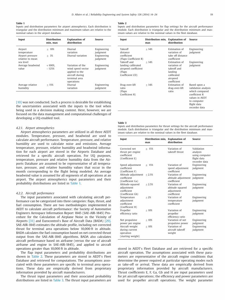
modules. Temperature, pressure, and headwind are used tocalculate aircraft performance. Temperature, pressure, and relativehumidity are used to calculate noise and emissions. Averagetemperature, pressure, relative humidity and headwind informa-tion for each airport are stored in the Airports Database andretrieved for a specific aircraft operation. For UQ purposes,temperature, pressure and relative humidity data from the Air-ports Database are assumed to be representative of all tempera-ture, pressure, and relative humidity values that occur in themonth corresponding to the flight being modeled. An averageheadwind value is assumed for all segments of all operations at anairport. The airport atmospherics input parameters and theirprobability distributions are listed in Table 1.

4.2.2. Aircraft performanceThe input parameters associated with calculating aircraft per-

formance can be categorized into three categories: flaps, thrust, andfuel consumption. There are two methodologies implemented inAEDT to calculate aircraft performance: the Society of AutomotiveEngineers Aerospace Information Report 1845 (SAE-AIR-1845) Pro-cedure for the Calculation of Airplane Noise in the Vicinity ofAirports [31] and Eurocontrol0s Base of Aircraft Data (BADA) [29].SAE-AIR-1845 estimates the altitude profile, including net correctedthrust for terminal area operations below 10,000 ft in altitude.BADA calculates the fuel consumption based on net corrected thrustoutput from the SAE-AIR-1845 algorithms. BADA also calculatesaircraft performance based on airframe (versus the use of aircraftairframe and engine in SAE-AIR-1845), and applied to aircraftoperations greater than 10,000 ft in altitude.

The flap input parameters and probability distributions areshown in Table 2. These parameters are stored in AEDT0s FleetDatabase and retrieved for computations. The assumptions asso-ciated with these parameters are specific to terminal area opera-tions. These data are empirically derived from proprietaryinformation provided by aircraft manufacturers.

The thrust input parameters and their associated probabilitydistributions are listed in Table 3. The thrust input parameters are

stored in AEDT0s Fleet Database and are retrieved for a specificaircraft operation. The assumptions associated with these para-meters are representative of the aircraft engine conditions thatdetermine the power required at particular operating modes suchas take-off or arrival. These data are empirically derived fromproprietary information provided by aircraft manufacturers.Thrust coefficients E, F, Ga, Gb and H are input parameters usedfor jet aircraft operations; the efficiency and power parameters areused for propeller aircraft operations. The weight parameter

Table 1Inputs and distribution parameters for airport atmospherics. Each distribution istriangular and the distribution minimum and maximum values are relative to thenominal values in the airport database.

Input Distributionmin, max

Explanation ofdistribution

Source

Airport 7 10% Diurnal Engineeringtemperature variation judgmentAirport pressure 7 3% Diurnal variation Engineeringrelative to mean judgmentsea levelAverage headwind þ100%, Variation of the Engineeringvalue �125% wind speed vector judgment

applied to theaircraft duringterminal areaoperations

Average relative 715% Diurnal Engineeringhumidity variation judgment

Table 2Inputs and distribution parameters for flap settings for the aircraft performancemodule. Each distribution is triangular and the distribution minimum and max-imum values are relative to the nominal values in the fleet database.

Input Distribution min,max

Explanation ofdistribution

Source

Takeoff 714% Estimation of Engineeringdistance variation of judgmentcoefficient take off distance(Flaps Coefficient B) coefficientTakeoff and 714% Estimation of Engineeringlanding calibrated variation of judgmentairspeed coefficient takeoff and(Flaps landingCoefficient CD) calibrated

airspeedcoefficient

Drag-over-lift 714% Estimation of Based upon aratio drag-over-lift validation analysis(Flaps ratio which comparedCoefficient R) coefficient R

values in AEDTto computerflight datarecorder data

Table 3Inputs and distribution parameters for thrust settings for the aircraft performancemodule. Each distribution is triangular and the distribution minimum and max-imum values are relative to the nominal values in the fleet database.

Input Distribution min,max

Explanation ofdistribution

Source

Corrected net 7 15% Variation of Validationthrust per engine takeoff thrust analysiscoefficient using computer(Coefficient E) flight data

recorder dataSpeed adjustment 7 15% Variation of Engineeringcoefficient speed adjustment judgment(Coefficient F) coefficientAltitude adjustment 72.5% Variation of Engineeringcoefficient altitude adjustment judgment(Coefficient Ga) coefficientAltitude-squared 72.5% Variation of Engineeringadjustment altitude squared judgmentcoefficient adjustment(Coefficient Gb) coefficientTemperature 72% Variation of Engineeringadjustment temperature judgmentcoefficient coefficient(Coefficient H)Propeller 710% Variation of Engineeringefficiency ratio propeller judgment

efficiency ratioNet propulsive 710% Variation of net Engineeringpower per engine propulsive power judgmentAircraft weight 710% Variation of Engineeringduring current aircraft takeoff judgmentoperation weight(starting weight)

D. Allaire et al. / Reliability Engineering and System Safety 126 (2014) 14–24 19

represents the weight of the aircraft. This value is determined bythe distance between the origin and destination airports referredto as the “stage length” of the aircraft operation.

Fuel consumption is calculated in AEDT by determining therequired thrust for a flight operation and assigning the appropriatethrust specific fuel consumption (TSFC) coefficients. To estimatefuel consumption, the SAE-AIR-1845 methodology calculates thethrust that corresponds to specific TSFC coefficients for an operat-ing mode such as departure or approach. The TSFC input para-meters and their probability distributions are listed in Table 4. TheTSFC input parameters are stored in AEDT0s Fleet Database and areretrieved for a specific aircraft operation.

4.2.3. Aircraft emissionsAircraft emissions are calculated by AEDT0s Aviation Emissions

Module (AEM) using the fuel consumption computed by the APMand the engine-specific emissions index stored in the Fleet Database.The input parameters and their probability distributions are listed inTable 5. Aircraft emission parameters are specific to aircraft operationmode, namely take-off, climb-out, approach and idle. The data arederived empirically from aircraft certification tests required by theInternational Civil Aviation Authority (ICAO). ICAO maintains adatabase of the certification data which includes data for fuel flow,carbon monoxide (CO), hydrocarbons (HCs), oxides of nitrogen (NOx),and smoke number (SN) (used for determining non-volatile particu-late matter) measured at the four landing and take-off cycle (LTO)power settings noted above.

The use of LTO cycle values of the ICAO emission indicescalculated at sea level static conditions introduces uncertainty inemissions inventory calculations because emissions must be

calculated with the Boeing Fuel Flow Method 2 (BFFM2) [13] atnon-reference conditions and power settings other than the fourICAO settings. The ICAO Committee on Aviation EnvironmentalProtection (CAEP) Working Group 3 has shown that BFFM2computations of NOx, CO, and HCs at non-reference conditionsand non-LTO-cycle power settings have an uncertainty of 10% [21].Also, the published literature indicates that engine-to-engineemission index variability can be estimated to be 16% for NOx,23% for CO, and 54% for HC at the 90% confidence interval for arepresentative sample of new, uninstalled engines [25]. Theemission indices in the ICAO emissions database do not includechanges in emission characteristics due to engine deteriorationover time. The effects of engine deterioration on NOx emissionsare estimated to be �1% to þ4% [26]. Engine deterioration effectsare applied to the final input distribution for NOx. These effectswere not applied to the final input distributions for CO and HC.

4.2.4. Aircraft noiseThe probability distributions for each input parameter for calcu-

lating the aircraft noise are listed in Table 6. Aircraft noise parametersare located within AEDT0s Fleet Database and are retrieved for aspecific aircraft operation on the geospatial location of the aircraft inreference to a grid point. Noise-power-distance (NPD) curves are afunction of engine power and distance from a particular grid pointand are developed according to SAE-AIR-1845. They are used todetermine noise level values by interpolating and/or extrapolating bythe net corrected thrust and slant distance between an aircraft andgrid point. The interpolation/extrapolation process is a piecewiselinear one between the engine power setting and the base-10

Table 4Inputs and distribution parameters for thrust specific fuel consumption settings forthe aircraft performance module. Each distribution is triangular and the distribu-tion minimum and maximum values are relative to the nominal values in the fleetdatabase.

Input Distribution min,max

Explanation ofdistribution

Source

Thrust specific 710% Estimation of Engineeringfuel consumption variation of TSFC judgmentCoeff1 (Boeing)-ConstantThrust specific 710% Estimation of Engineeringfuel consumption variation of TSFC judgmentCoeff2 (Boeing)-MachThrust specific 710% Estimation of Engineeringfuel consumption variation of TSFC judgmentCoeff3 (Boeing)-AltitudeThrust specific 710% Estimation of Engineeringfuel consumption variation of TSFC judgmentCoeff4 (Boeing)-Thrust1st thrust specific 710% Estimation of Engineeringfuel consumption variation of TSFC judgmentcoefficient(TSFC BADA 1)2nd thrust specific 710% Estimation of Engineeringfuel consumption variation of TSFC judgmentcoefficient(TSFC BADA 2)1st descent fuel 710% Estimation of Engineeringflow coefficient variation of TSFC judgment(TSFC BADA 3)2nd descent fuel 710% Estimation of Engineeringflow coefficient variation of TSFC judgment(TSFC BADA 4)

Table 5Inputs and distribution parameters for emission indices for the aircraft emissionsmodule. Each distribution is triangular and the distribution minimum and max-imum values are relative to the nominal values in the fleet database.

Input Distributionmin, max

Explanation ofdistribution

Source

ICAO reference 75% Variation of ICAO Engineeringfuel flow fuel flow judgmentICAO reference 726% Variation of ICAO Validation analysisemissions index carbon monoxide while establishingfor CO (CO EI) emissions indices ICAO certification

procedureICAO reference 755% Variation of ICAO Validation analysisemissions index hydrocarbon while establishingfor HC (HC EI) emissions indices ICAO certification

procedureICAO reference 724% Variation of ICAO Validation analysisemissions index nitrogen oxides while establishingfor NOx (NOx EI) emissions indices ICAO certification

procedureICAO reference 73 Estimation of Validation analysissmoke number (SN) variation of ICAO while establishing

smoke number ICAO certificationprocedure

Table 6Inputs and distribution parameters for the aircraft noise module. Each distributionis triangular and the distribution minimum and maximum values are relative to thenominal values in the fleet database.

Input Distribution min, max Explanation ofdistribution

Source

Noise-power 71.5 dB Variation of noise Noise certificationdistance (NPD) certification data guidelinescurves

D. Allaire et al. / Reliability Engineering and System Safety 126 (2014) 14–2420

logarithm of distance. Noise certification values are reported withinan error of þ/� 1.5 decibels (dB) [14].

4.3. UQ results: fuel burn and emissions

Fig. 4 shows the output histograms of fuel burn for JFK, ATL andTEB, respectively. Table 7 lists the mean, standard deviation, andcoefficient of variation for the fuel burn distributions in each case.Even accounting for the many uncertain input parametersdescribed in the previous section, AEDT estimates of fuel burnhave relatively low uncertainty, with standard deviations of lessthan 2% of the mean values for all airports analyzed. Fig. 5 showsthe total sensitivity indices (TSIs) for those input parameters thatcontributed the most to the fuel burn output variance for eachairport analyzed. The biggest contributor to the variance for fuelburn across all airports is aircraft weight. The ranking of the TSIvalues for the other parameters vary for each of the airportsanalyzed. The TSFC BADA 1 coefficient was the second highestcontributor to the variance for JFK and TEB; however, for ATL itwas the fifth highest contributor. This difference is due to fleet mixdifferences between the three airports. The fleet mix for JFKconsists of many aircraft that utilized the BADA TSFC coefficients.

ATL has a large portion of Boeing aircraft within its fleet, whichutilize the Terminal TSFC coefficients.

Table 7 also shows the mean, standard deviation, and coeffi-cient of variation for the distributions of NOx, CO, HC, andparticulate matter (PM) emissions. It can be seen that uncertaintyin emission estimates is generally higher than for fuel burnestimates. This is because emission estimates are subject to theadditional uncertainty stemming from the emissions indices. HCemissions show the largest coefficient of variation results. Fig. 6shows the TSI values for the most significant contributors tooutput variance in HC emissions. We see that uncertainty in HCemissions is dominated by the HC Emissions Index (EI). For JFK,temperature and pressure also contribute a small amount to theHC emissions variance. Fig. 7 shows sensitivity indices for PMemissions. In this case, there is not a single dominating inputparameter. Aircraft weight is important, as there are variouscoefficients in the models of aircraft and engine performance.

4.4. UQ results: noise

We present noise uncertainty analysis and sensitivity analysisresults for JFK airport only. The output of interest in this case is theSound Exposure Level (SEL), which is a measure of the total noiseenergy produced by a noise event. The noise analysis wasconducted using an 81-point evenly spaced receptor grid that

Fig. 4. Fuel burn output distributions for JFK (upper left), ATL (upper right), and TEB (lower).

Table 7Fuel burn and emissions statistics for JFK, ATL and TEB.

Output Airport JFK ATL TEB

Fuel burn Mean (Mg) 1005 1081 83Standard deviation (Mg) 9 12 1.5Coefficient of variation (%) 0.9 1.2 1.8

NOx Mean (kg) 14,116 14,777 883Standard deviation (kg) 362 470 41Coefficient of variation (%) 2.6 3.2 4.6

CO Mean (kg) 12,368 12,513 1720Standard deviation (kg) 316 366 52Coefficient of variation (%) 2.6 2.9 3.0

HC Mean (kg) 1655 1838 653Standard deviation (kg) 77 122 74Coefficient of variation (%) 4.6 6.6 11.3

PM Mean (kg) 304 397 37Standard deviation (kg) 5.6 9.0 1.2Coefficient of variation (%) 1.8 2.3 3.3

Fig. 5. Fuel burn TSI values for JFK, ATL and TEB.

D. Allaire et al. / Reliability Engineering and System Safety 126 (2014) 14–24 21

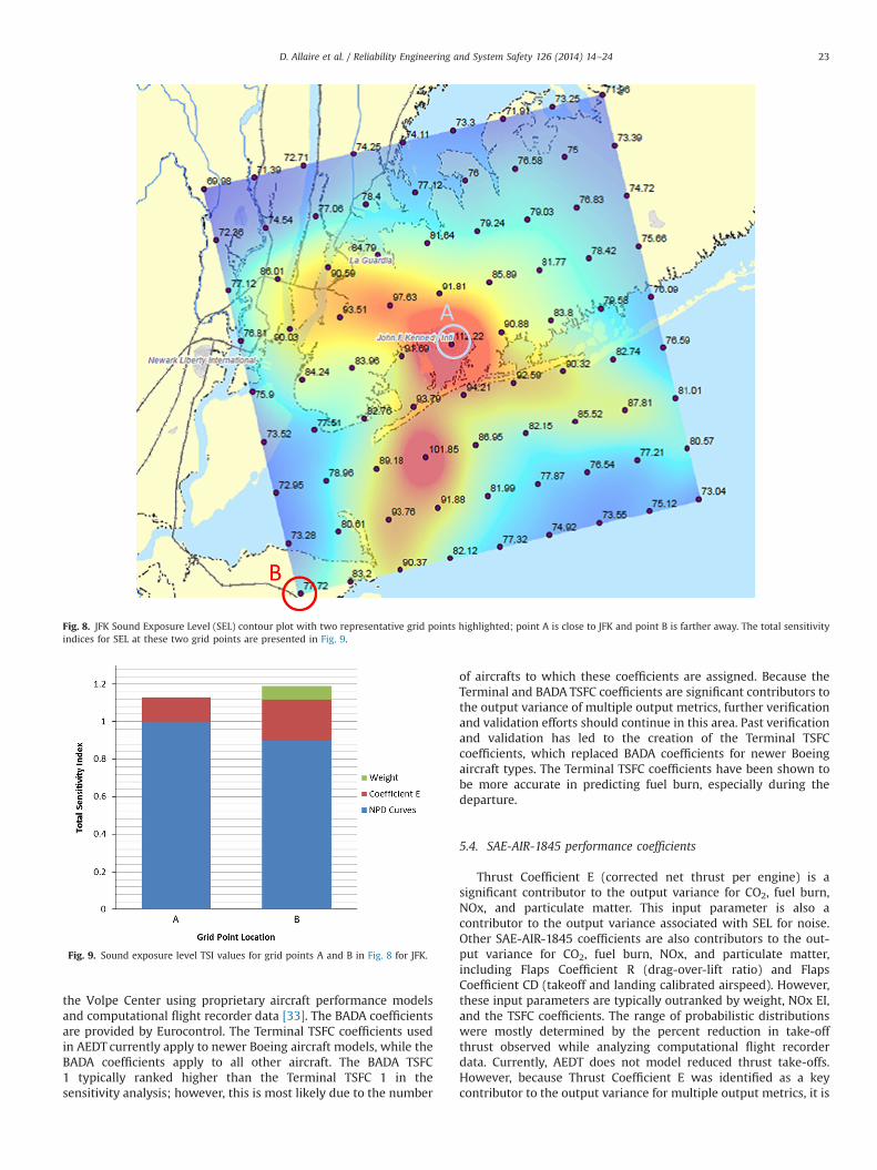
covers a 20�20 nautical mile area around JFK airport. Fig. 8depicts a noise contour plot of the mean SEL values resulting fromthe uncertainty analysis, conducted via Monte Carlo simulation.Sensitivity analysis computes TSI values for each grid point. Thenumerical values of the sensitivity indices are not shown here dueto the large number of grid points. Fig. 9 presents the totalsensitivity indices for a grid point near JFK (point A in Fig. 8)and a grid point farther away from JFK (point B in Fig. 8). Thesensitivity analysis for these grid points is typical for all grid pointsand reveals that the uncertainty surrounding the noise-power-distance (NPD) curves is the most significant contributor to SELvariance. TSI values for NPD curves were typically above 0.95 foreach grid point analyzed. Thrust Coefficient E was the secondhighest contributor to the output variance, with TSI values around0.05 at each grid point. The analysis also showed small contribu-tions ðo1%Þ to SEL variance from aircraft weight and atmospherictemperature parameters.

5. Discussion

The sensitivity and uncertainty analyses conducted for AEDThave identified input parameters that contribute the most tooutput variance and uncertainty for emissions, fuel burn, andnoise. Even though the scope of these analyses was limited to theuse of the AEDT Alpha version, the results are generally applicableto more advanced versions of AEDT, because the core algorithmsand associated assumptions are carried forward in those releasesof AEDT. In total, 29 individual input parameters contributedsignificantly to the output variances across all emissions and noiseoutput metrics. Only 12 of those input parameters are significantcontributors to the output variances of all the emission metrics atthe airport level within the terminal area. Only two parameterscontributed to the output variance for noise. While the discussion

below focuses on the technical details of AEDT models, it demon-strates more generally how the UQ analyses support the specificgoals described in Section 1. In particular, the uncertainty analysisand sensitivity analysis results highlight the most importantassumptions within the models, identify gaps in the models, andindicate important areas for future tool development.

5.1. Emissions Indices (EIs)

The ICAO engine EI uncertainties were found to be the maincontributors to output variance for NOx, HC and CO emissions. Asshown in Table 5, the distributions assumed for the EIs weretriangular with upper/lower bounds of 24% of the mean value forNOx, 26% for CO, and 55% for HC. These EI uncertainties includeengine-to-engine variations as well as the uncertainty in BoeingFuel Flow Method 2 (BFFM2) calculations. These values werederived from published data based on the fuel venting and exhaustemissions requirements associated with the engine certificationprocess [15]. In the context of engine emissions certification, theDp/Foo value represents the mass of any gaseous pollutant emittedduring the LTO cycle divided by an engines rated thrust output.The minimum requirement for engine certification is that a singleengine is tested three times; the mean Dp/Foo values are calcu-lated from those three tests. To determine if the engine type meetsthe certification emission requirements, the mean Dp/Foo valuesare adjusted upward by 16% for NOx, 23% for CO, and 54% for HC tocalculate the characteristic Dp/Foo. This value is then compared tocertification emission standards. The characteristic Dp/Foo valueaccounts for the uncertainty associated with engine-to-engine EIvariability; if the characteristic Dp/Foo for the engine does notmeet the certification emission standards then additional enginesof that same model number are tested to reduce the overalluncertainty in calculating the characteristic Dp/Foo values. Theseadjustment factors are based on certification-like studies thatwere conducted in the 1970s [25]. They may be consideredconservative due to how modern aircraft engines have evolved.Also, all EI and SN values have four certification points for take-off(100% power), climb-out (85% power), approach (30% power), andidle (7% power). For this analysis, the same probability distributionwas used for each power setting, although in reality the EIuncertainty associated with each power setting may vary. A betterunderstanding for which power setting the EI uncertainty is mostimportant may provide valuable guidance to mitigating the effectsof this uncertainty.

5.2. Aircraft weight

Aircraft weight was found to be a significant contributor to theoutput variance for CO2, fuel burn, NOx, and particulate matter.AEDT determines aircraft weight based upon origin-to-destinationstage length distance. Each aircraft can have multiple stage lengthdistances based upon range and purpose. Our analysis used atriangular distribution to represent weight uncertainty, with upperand lower bounds of 10% of the mean value. Because the aircraftweight was observed to be such a large contributor to the outputvariance of multiple output metrics, this is a valuable area inwhich to invest resources to better understand the associateduncertainties. For example, computational fight recorder datacould be analyzed to better characterize stage length weight andits variations.

5.3. Terminal and BADA TSFC coefficients

The Terminal and BADA TSFC 1 coefficients are significantcontributors to the output variance of CO2, fuel burn, NOx, andparticulate matter. The Terminal coefficients were developed by

Fig. 6. Hydrocarbon emission TSI Values for JFK, ATL and TEB.

Fig. 7. Particulate matter emission TSI Values for JFK, ATL and TEB.

D. Allaire et al. / Reliability Engineering and System Safety 126 (2014) 14–2422

the Volpe Center using proprietary aircraft performance modelsand computational flight recorder data [33]. The BADA coefficientsare provided by Eurocontrol. The Terminal TSFC coefficients usedin AEDT currently apply to newer Boeing aircraft models, while theBADA coefficients apply to all other aircraft. The BADA TSFC1 typically ranked higher than the Terminal TSFC 1 in thesensitivity analysis; however, this is most likely due to the number

of aircrafts to which these coefficients are assigned. Because theTerminal and BADA TSFC coefficients are significant contributors tothe output variance of multiple output metrics, further verificationand validation efforts should continue in this area. Past verificationand validation has led to the creation of the Terminal TSFCcoefficients, which replaced BADA coefficients for newer Boeingaircraft types. The Terminal TSFC coefficients have been shown tobe more accurate in predicting fuel burn, especially during thedeparture.

5.4. SAE-AIR-1845 performance coefficients

Thrust Coefficient E (corrected net thrust per engine) is asignificant contributor to the output variance for CO2, fuel burn,NOx, and particulate matter. This input parameter is also acontributor to the output variance associated with SEL for noise.Other SAE-AIR-1845 coefficients are also contributors to the out-put variance for CO2, fuel burn, NOx, and particulate matter,including Flaps Coefficient R (drag-over-lift ratio) and FlapsCoefficient CD (takeoff and landing calibrated airspeed). However,these input parameters are typically outranked by weight, NOx EI,and the TSFC coefficients. The range of probabilistic distributionswere mostly determined by the percent reduction in take-offthrust observed while analyzing computational flight recorderdata. Currently, AEDT does not model reduced thrust take-offs.However, because Thrust Coefficient E was identified as a keycontributor to the output variance for multiple output metrics, it is

Fig. 8. JFK Sound Exposure Level (SEL) contour plot with two representative grid points highlighted; point A is close to JFK and point B is farther away. The total sensitivityindices for SEL at these two grid points are presented in Fig. 9.

Fig. 9. Sound exposure level TSI values for grid points A and B in Fig. 8 for JFK.

D. Allaire et al. / Reliability Engineering and System Safety 126 (2014) 14–24 23

suggested that further research efforts be conducted to investigatethe potential impact of AEDT not having this capability.

5.5. NPD curves

The NPD curves are the most significant contributor to thevariability of SEL noise output. Atmospheric parameters, such astemperature, pressure, and relative humidity, do not significantlycontribute to the output variance. Like the ICAO EI values, whichare based upon the emissions certification process, the currentNPD generation process is unlikely to change. For this analysis,each point along an NPD curve was varied independently. Analternate approach would be to shift all of the points along theNPD curve in unison. Future analysis should determine theappropriateness of each approach. Items that were not addressedwith this analysis include the variation of type of profile or track.Since both items affect the location of the aircraft, their variation(reflecting day-to-day variation at a given airport) would likelycontribute further to SEL variance. In addition, our analysis used81-points in the receptor grid. Future analyses will assess whetheroutput variance contributions change when more grid pointscloser to the airport are considered.

6. Conclusions and future work

This paper has presented methodology and results for uncer-tainty quantification of a real-world complex system modelingtool. The approaches described in the paper overcome the com-plexities of long run times and massive input/output datasets,using a combination of surrogate modeling and grouped sensitiv-ity analysis. Several general conclusions can be drawn from the UQeffort presented here. First, sensitivity analysis on a black-box codeis a systematic and effective means of identifying high priorityareas for future research as well as insignificant factors that can befixed to nominal values. For models with high-dimensional inputfactors, the latter is an essential part of managing database andanalysis complexity. Second, surrogate models are essential forachieving UQ at scale in complex tools. Third, the overall AEDTdevelopment process benefited from conducting UQ concurrentlywith the tool development. Developers were able to include in thetoolset the necessary software and database attributes to create aUQ-enabled tool. In return, the concurrent UQ analysis was able toidentify and feed back analysis limitations, in time to have impacton the tool development. Although challenging to manage, con-current development and UQ assessment processes bring signifi-cant benefit.

Acknowledgments

This work was funded by the US Federal Aviation AdministrationOffice of Environment and Energy under FAA Contract Number:DTFAWA-05-D-00012, Task Order Nos. 0002, 0008, and 0009. Theproject was managed by Maryalice Locke, FAA. Any opinions,findings, and conclusions or recommendations expressed in thismaterial are those of the authors and do not necessarily reflect theviews of the FAA.

References

[1] Allaire D, Willcox K. Surrogate modeling for uncertainty assessment withapplication to aviation environmental system models. AIAA J 2010;48(8):1791–803.

[2] Allaire D, Willcox K. A variance-based sensitivity index function for factorprioritization. Reliab Eng Syst Saf 2012;107(November):107–14.

[3] Amaral S, Allaire D, Willcox K. A decomposition approach to uncertaintyanalysis of multidisciplinary systems. In: Proceedings of the 14th AIAA/ISSMOmultidisciplinary analysis and optimization conference, No. AIAA-2012-5563,Indianapolis, IN; 2012 September 17–19.

[4] Babuška I, Nobile F, Tempone R. A stochastic collocation method for ellipticpartial differential equations with random input data. SIAM J Numer Anal2007;45(3):1005–34.

[5] Baratelli F, Giudici M, Vassena C. A sensitivity analysis for an evolution modelof the Antarctic ice sheet. Reliab Eng Syst Saf 2012;107.

[6] Boeker E, Dinges E, He B, Fleming G, Roof C, Gerbi P, et al. Integrated noisemodel (INM) version 7.0 technical manual; 2008. FAA-AEE-08-01.

[7] Bui-Thanh T, Willcox K, Ghattas O. Parametric reduced-order models forprobabilistic analysis of unsteady aerodynamic applications. AIAA J 2008;46(10):2520–9.

[8] Cacuci D. Sensitivity and uncertainty analysistheory. Boca Raton, FL: Chapman& Hall/CRC; 2003.

[9] Chan K, Saltelli A, Tarantola S. Sensitivity analysis of model output: variance-based methods make the difference. In: Proceedings of the 1997 wintersimulation conference; 1997.

[10] Cooke R, Goosens L. TU Delft expert judgment data base. Reliab Eng Syst Saf2008;93(5):657–74.

[11] Cover T, Thomas J. Elements of Information Theory. Hoboken, NJ: John Wiley &Sons, Inc.; 1991.

[12] CSSI. Emissions and dispersion modeling system (EDMS) version 5 technicalmanual; 2009. FAA-AAA-07-07.

[13] DuBois D, Paynter G. Fuel flow method 2 for estimating aircraft emissions. SAEtechnical paper 2006-01-1987; 2006.

[14] Federal Aviation Administration. AC36-4B noise certification handbook; 1988.[15] Federal Aviation Administration. Fuel venting and exhaust emission require-

ments for turbine engine powered engines. Advisory circular 34-1B; 2003.[16] Federal Aviation Administration. Aviation environmental design tool (AEDT)

2a user guide; March 2012.[17] Federal Aviation Administration. Aviation environmental design tool (AEDT)

2a uncertainty quantification report; August 2013.[18] Forrester A, Sóbester A, Keane A. Engineering design via surrogate modelling:

a practical guide. Chichester, UK: John Wiley & Sons; 2008.[19] Helton J, Hansen C, Sallaberry C. Uncertainty and sensitivity analysis in

performance assessment for the proposed high-level radioactive waste repo-sitory at Yucca Mountain, Nevada. Reliab Eng Syst Saf 107; 2012.

[20] Homma T, Saltelli A. Importance measures in global sensitivity analysis ofnonlinear models. Reliab Eng Syst Saf 1996;52:1–17.

[21] ICAO-CAEP. Guidance on the use of LTO emissions certification data for theassessment of operational impacts. Working group 3; 2004.

[22] Jaynes E. Probability theory: the logic of science. Cambridge, United Kingdom,New York: Cambridge University Press; 2003.

[23] Johnson D. The triangular distribution as a proxy for the beta distribution inrisk analysis. The Statistician 1997;46(3):387–98.

[24] Kim B, Fleming G, Lee J, Waitz I, Clarke J, Balasubramanian S, et al. System forassessing aviation0s global emissions (SAGE). Part 1. Model description andinventory results. Transp Res Part D: Transp Environ 2007;12(5):325–46.

[25] Lee J. Modeling aviation0s global emissions, uncertainty analysis, and applica-tions to policy (Ph.D. thesis). Massachusetts Institute of Technology, Cam-bridge, MA; 2005.

[26] Lukachko S, Waitz I. Effects of engine aging on aircraft NOx emissions. In:Proceedings of the ASME turbo expo, ASME 97-GT-386; 1997.

[27] NASA. Standards for models and simulations. National Aeronautics and SpaceAdministration, Technical Standard NASA-STD-7009; 2008.

[28] National Research Council. Assessing the reliability of complex models:Mathematical and statistical foundations of verification, validation, anduncertainty quantification. The National Academies Press, Washington, DC;2012.

[29] Nuic A. User manual for the base of aircraft data (BADA) revision 3.6; 2004.[30] Oladyshkin S, Nowak W. Data-driven uncertainty quantification using the

arbitrary polynomial chaos expansion. Reliab Eng Syst Saf 2012;106.[31] SAE. SAE-AIR-1845. Society of Automotive Engineers A-21 Committee; 1986.[32] Saltelli A, Ratto M, Andres T, Campolongo F, Cariboni J, Gatelli D, et al. Global

sensitivity analysis: the primer. West Sussex, England: John Wiley & Sons, Ltd.,2008.

[33] Senzig D, Fleming G, Iovinelli R. Modeling of terminal-area airplane fuelconsumption. J Aircr 2009;46(4):1089–93.

[34] Sobol0 I. Theorems and examples on high dimensional model representation.Reliab Eng Syst Saf 2003;79:187–93.

[35] Thompson T, Augustine S, DiFelichi J, Graham M, Warren D. Noise integratedrouting system user0s guide version 7.0a.1;2009.

[36] Williams T. Practical use of distributions in network analysis. J Oper Res Soc1992;43(3):265–70.

[37] Xiu D, Karniadakis G. The Wiener–Askey polynomial chaos for stochasticdifferential equations. SIAM J Sci Comput 2002;24(2):619–44.

[38] Zentner I, Tarantola S, de Rocquigny E. Sensitivity analysis for reliable designverification for nuclear turbosets. Reliab Eng Syst Saf 2011;96.

D. Allaire et al. / Reliability Engineering and System Safety 126 (2014) 14–2424