reliable calculations of heat and fluid flow during ... · absorption coefficient cannot be...

WELDING RESEARCH

-s101WELDING JOURNAL

ABSTRACT. During conduction modelaser beam welding, the quality of numer-ical simulation of heat transfer and fluidflow in the weld pool is significantly af-fected by the uncertainty in the values ofabsorptivity, effective thermal conductiv-ity, and effective viscosity that cannot beeasily prescribed from fundamental prin-ciples. Traditionally, values of these para-meters are either prescribed based on ex-perience or adjusted by trial and error.This paper proposes a deterministic ap-proach to improve reliability of heat trans-fer and fluid flow calculations. The ap-proach involves evaluation of theoptimized values of absorptivity, effectivethermal conductivity, and effective viscos-ity during conduction mode laser beamwelding from a limited volume of experi-mental data utilizing an iterative multi-variable optimization scheme and a nu-merical heat transfer and fluid flow model.The optimization technique minimizes theerror between the predicted and the mea-sured weld dimensions by considering thesensitivity of weld dimensions with respectto absorptivity, effective thermal conduc-tivity, and effective viscosity. Five sets ofmeasured weld pool dimensions corre-sponding to five different welding condi-tions were utilized for the optimization.However, the procedure could identify theoptimized values of the three uncertainparameters even with only three sets ofmeasured weld pool dimensions.

Introduction

Since the temperature and velocityfields in the weld pool are difficult to mea-sure experimentally (Refs. 1–7), these im-portant variables are often estimated bynumerically solving the equations of con-servation of mass, momentum, and en-ergy. In recent years, the numerically com-puted temperature fields have beenutilized to estimate weld pool dimensions(Refs. 4–7) and understand weld metalphase composition (Refs. 8–11), grainstructure (Refs. 10, 11), inclusion struc-ture (Refs. 12–14), and weld metal com-position changes owing to both vaporiza-tion of alloying elements (Refs. 15, 16) anddissolution of gases (Refs. 17, 18).

The transport phenomena-based nu-merical models have been continually up-dated to include more detailed and realis-tic descriptions of component physicalprocesses for simple(Refs. 19–22) as wellas for complex weld joint geometries (Ref.23). In recent years, these models have be-come relatively easy to use because of ad-vances in computational hardware andsoftware. However, these powerful nu-merical heat transfer and fluid flow mod-els have not found widespread use in man-

ufacturing or design applications. An im-portant difficulty is the uncertainty in-volved in specifying some of the necessaryinput variables such as absorptivity, effec-tive thermal conductivity, and effectiveviscosity. Although the time-tested physi-cal laws such as the equations of conser-vation of mass, momentum, and energyprovide a reliable phenomenologicalframework for calculations, the reliabilityof the numerical process models greatlydepends on the accuracy of several inputparameters.

Many input parameters necessary forthe numerical simulation of heat transferand fluid flow in conduction-mode linearlaser beam welding can be readily speci-fied. These include welding speed, beampower, beam diameter, and thermophysi-cal properties of the material beingwelded (Refs. 19, 24). However, the valuesof absorptivity, effective thermal conduc-tivity and effective viscosity cannot bespecified from fundamental principles(Refs. 2, 24–30). For example, absorptivitydepends on the chemical composition ofthe substrate, the surface finish, lasermode, and the prevailing temperature dis-tribution on the weld pool. As a result, theabsorption coefficient cannot be esti-mated theoretically with high reliability.However, an accurate value of absorptiv-ity is critical for the dependable estimationof the rate of heat absorption. Similarly,appropriate values of effective thermalconductivity and effective viscosity areneeded for the reliable modeling of thehigh rates of transport of heat, mass, andmomentum in weld pools with strong fluc-tuating velocities (Ref. 25). Enhanced val-ues of liquid thermal conductivity and vis-cosity have been frequently used to takeinto account the effects of the fluctuating

SUPPLEMENT TO THE WELDING JOURNAL, JULY 2005Sponsored by the American Welding Society and the Welding Research Council

Reliable Calculations of Heat and Fluid Flowduring Conduction Mode Laser Welding

through Optimization of UncertainParameters

A deterministic approach is proposed to improve reliability of heat transfer and fluid flow calculations

BY A. DE AND T. DebROY

KEY WORDS

LaserLaser Beam WeldingHeat TransferFluid FlowConduction Mode

A. DE ([email protected]) is with the Me-chanical Engineering Department, IITBombay, Mumbai, India. T. DebROY ([email protected]) is with the Department ofMaterial Science and Engineering, ThePennsylvania State University, UniversityPark, Pa.

De---7_05 6/6/05 4:07 PM 01

WELDING RESEARCH

JULY 2005-s102

components of velocities in the weld pool.In some cases, the two-equation k-e tur-bulence model has also been used in esti-mating the effective viscosity and effectivethermal conductivity in the weld pool(Refs. 26–28). However, the two-equationk-e turbulence model contains several em-pirical constants that were originally esti-mated from parabolic fluid flow data inlarge systems. As a result, its applicabilityfor the recirculating flow in small scale sys-tems has not been adequately tested.Since the effective thermal conductivityand viscosity depend on the turbulent ki-netic energy and other properties of con-vection, these parameters are system

properties (Refs. 1, 2, 24–30) and their val-ues depend on welding conditions, partic-ularly the heat input.

The values of effective viscosity andthermal conductivity have been determinedin this work as a function of heat input froma limited volume of measured weld pool di-mensions for conduction mode linear laserbeam welding (Ref. 24) utilizing an opti-mization algorithm and a numerical heattransfer and fluid flow model. In contrastwith the effective viscosity or the effectivethermal conductivity, the laser beam ab-sorption coefficient is a materials property.Although it varies with temperature, the ex-tent of the variation is normally muchsmaller than those of the effective thermalconductivity or the effective viscosity. It hasbeen taken as a constant in this work forsimplicity. The optimization algorithm min-imizes the error between the predicted andthe experimentally observed penetrationsand the weld widths by considering the sen-sitivity of the computed weld pool dimen-sions with respect to the absorptivity, effec-tive thermal conductivity, and effectiveviscosity. The sensitivity terms are calcu-lated by running the heat transfer and fluid

flow model several times for each measure-ment considering small changes in the ab-sorptivity, effective thermal conductivity,and effective viscosity (Refs. 29, 30).

The approach determines the values ofabsorptivity, effective viscosity and ther-mal conductivity in an iterative mannerstarting from a set of their initial guessedvalues. In order to include the effects oflaser power, spot diameter, and weldingspeed into one convenient variable duringoptimization, a nondimensional heatinput variable, NHI, is defined as

(1)

where P is the laser power (W), rb the spotradius (m), v the welding velocity (m◊s–1),CPS the specific heat of the solid metal(J.kg–1.K–1), r the density (kg.m–3), L thelatent heat of fusion (J.kg–1) and TL and Taare the liquidus and ambient tempera-tures (K), respectively. In Equation 1, thenumerator represents the available laserpower per unit volume and the denomina-tor depicts the enthalpy required to heat aunit volume of metal from ambient tem-perature to liquidus temperature. The nu-merator in Equation 1 when multiplied bythe absorptivity, h, provides the absorbedheat per unit volume. The optimizationapproach identifies a single value of ab-sorptivity and a linear trend of effectivethermal conductivity and effective viscos-ity with NHI from a limited volume of mea-surements.

The work presented in this manuscriptrepresents a significant improvement overthe previous (Refs. 31–35) reverse model-

N

P

v

C T T LHI

rb

PS L a=

◊

-( ) +p

r r

2

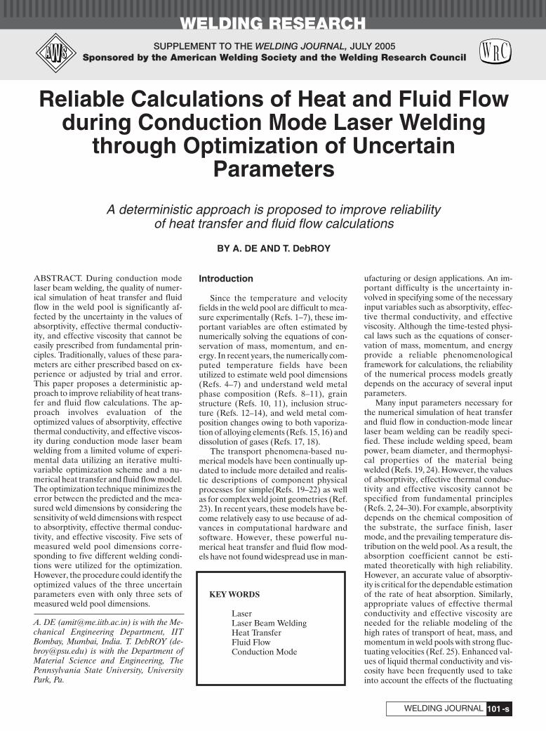
Fig. 1 — Influence of k* and m* on (i) p* and (ii) w* with assumed absorptivity (h) of 0.30. Welding parameters: P = 3200 W, v = 3.33 mm/s (NHI = 21.90).

Table 1 — Measured Weld Dimensions, Welding Parameters (Ref. 24), and Heat Input Index

Data Laser Weld Spot NHI Weld WeldSet Power Velocity Radius Penetration WidthIndex (W) (mm.s–1) (mm) (mm) (mm)

1 3500 8.33 1.3 9.67 1.00 4.002 5000 8.33 1.3 14.97 1.25 5.253 3200 3.33 1.4 21.90 1.75 4.004 4800 3.33 1.4 32.90 2.50 6.005 5000 3.33 1.3 34.53 2.25 6.75

Table 2 — Chemical Composition (wt-%) ofHigh-Speed Steel Used for WeldingExperiments(a)

C Cr W Mo V Co Mn

0.92 3.88 6.08 4.9 1.73 0 0.26Si S Ni P Cu Al Fe0.23 0.001 0.24 0.024 0.20 0.019 Bal.

(a) for data set index 1, 2, and 5 (Ref. 24).

m m

De---7_05 6/6/05 4:07 PM Page 102

WELDING RESEARCH


ing work in welding reported in the litera-ture. First, unlike the previous efforts, awell-tested, three-dimensional numericalheat transfer and fluid flow model is usedto compute the weld pool geometry. Thisis significant, because previous researchhas shown the importance of convectiveheat transfer in the weld pool. Second, themodel input and the computed weld poolgeometry are related by a rigorous phe-nomenological framework of the conser-vation of mass, momentum, and energyused in the optimization algorithm. Theoptimized values of absorptivity, effectivethermal conductivity, and effective viscos-ity were tested by comparing the com-puted weld dimensions with the corre-sponding experimentally determinedvalues (Ref. 4).

The effect of volume of data on theoutcome of the optimization was exam-ined. First, the optimization was doneusing five sets of measured weld pool di-mensions. Second, the optimization wasalso carried out with only three measureddata sets of weld pool dimensions. The op-timized values of the uncertain variableswere almost identical in both cases.

Heat Transfer and Fluid FlowSimulation

Table 1 depicts five sets of measure-ments of weld dimensions and the corre-sponding welding parameters that havebeen used in the present investigation.The chemical compositions of the steelsused are presented in Tables 2 and 3. Thesteel compositions conform to two differ-ent grades of high-speed steel (Ref. 24).The thermophysical properties of these

steels are given in Tables 4 and 5. The flowof liquid metal in the weld pool in a three-dimensional cartesian coordinate systemis represented by the following momen-tum conservation equation (Refs. 4, 21,22, 36):

(2)

where r is the density, t is the time, xi is thedistance along the i = 1, 2 and 3 directions,uj is the velocity component along the j di-rection, m is the effective viscosity, and Sjis the source term for the jth momentumequation and is given as (Refs. 21, 22)

(3)

where p is the pressure, fL is the liquidfraction, B is a constant introduced to

avoid division by zero, C (=1.6 ¥ 104) is aconstant that takes into account mushyzone morphology and Sbj represents boththe electromagnetic and buoyancy sourceterms. The third term on the right-handside (RHS) represents the frictional dissi-pation in the mushy zone according to theCarman-Kozeny equation for flowthrough a porous media (·Refs. 37, 38).The pressure field was obtained by solvingthe following continuity equation simulta-neously with the momentum equation

(4)

∂( )∂

=ruxi

i0

Sp

x x

u

x

Cf

f B

u Uu

xSb

jj j

j

j

L

L

ji

ij

= - ∂∂

+ ∂∂

∂

∂

Ê

ËÁÁ

ˆ

¯˜ -

-( )+

Ê

Ë

ÁÁÁÁ

ˆ

¯

˜˜˜

- ∂∂

+

m

r1

2

3

r r m∂

∂+

∂( )∂

= ∂∂

∂∂

Ê

ËÁˆ

¯+

u

t

u u

x x

u

xSj i j

i i

j

ij

Fig. 2 — Influence of k* and m* on O(f) with assumed absorptivity (h) of0.30. Welding parameters: P = 3200 W, v = 3.33 mm/s (NHI = 21.90).

Fig. 3 —Influence of k* and m* on O(f) with assumed absorptivity (h) of0.30. Welding parameters: P = 5000 W, v = 8.33 mm/s (NHI = 14.97).

Table 3 — Chemical Composition (wt-%) ofHigh-Speed Steel Used for WeldingExperiments(a)

C Cr W Mo V Co Mn

0.21 0.21 <0.05 0.05 <0.02 <0.05 1.52Si S Ni P Cu Al Fe0.36 0.006 0.14 <0.005 0.14 0.01 Bal.

(a) for data set index 3 and 4 (Ref. 24).

Table 4 — Data Used for Calculations ofTemperature and Velocity Fields(a)

Physical Property Value

Liquidus temperature, TL (K) 1700.0Solidus temperature, TS (K) 1480.0Ambient temperature, Ta (K) 293.0Density of liquid metal, r (kg/m3) 8.1 ¥ 103

Thermal conductivity of solid, 25.08ks (W m–1 K–1)Thermal conductivity of liquid, 25.08kL (W m–1 K–1)Specific heat of solid, 711.0CPS (J kg–1 K–1)Specific heat of liquid, 711.0CPL (J kg–1 K–1)Temperature coefficient of –0.5 ¥ 10–3

surface tension, dg/dT (N m–1 K–1)Coefficient of thermal 1.5 ¥ 10–6

expansion, b (K–1)Viscosity of molten iron 6.7 ¥ 10–3

at 1823 K, m fl (kg.m–1s–1)

(a) for data set index 1, 2, and 5 (Ref. 24).

De---7_05 6/6/05 4:07 PM Page 103

WELDING RESEARCH

JULY 2005-s104

The total enthalpy H is represented by asum of sensible heat h and latent heat con-tent DH, i.e., H = h + DH where h = ∫CpdT, Cp is the specific heat, T is the tem-perature, DH = fLL, L is the latent heat offusion and the liquid fraction fL is assumedto vary linearly with temperature in themushy zone ·(Ref. 4).

(5)

where TL and TS are the liquidus andsolidus temperature, respectively. The ther-mal energy transport in the weld workpiececan be expressed by the following modified

energy equation (Refs. 4, 21):

(6)

where k is the thermal conductivity. Theeffective thermal conductivity in the liquidweld pool is also a property of the specificwelding system and not a fundamentalproperty of the liquid metal. Therefore,

the value of the effective thermal conduc-tivity is not known. Since the weld is sym-metrical about the weld centerline onlyhalf of the workpiece is considered. Theweld top surface is assumed to be flat. Thevelocity boundary condition is given as(Ref. 4)

(7)

where u, v, and w are the velocity compo-nents along the x, y, and z directions, re-

m g

m g

∂∂

= ∂∂

∂∂

= ∂∂

=

uz

fddT

Tx

vz

fddT

Ty

w

L

L

0

r r

r r r

r

∂∂

+∂( )∂

= ∂∂

∂∂

Ê

ËÁ

ˆ

¯˜

- ∂∂

-∂( )

∂- ∂

∂

- ∂∂

ht

u h

x xkC

hx

Ht

u H

xU

hx

UHx

i

i i p i

i

i i

i

D D

Df

T TT T

T T TLS

L Ss LT T

T T

S

L=

--

ÏÌÔ

ÓÔ£ £<

>

0

1

Fig. 4 — Progress of calculation with four sets of intitial guessed valuesusing (i) LM method, (ii) CGPR method, and (iii) CGFR method. The ini-tial guessed values are presented in Table 6.

Fig. 5 — Estimated optimum values of k* and m* for all values of NHI. (Op-timum value of h = 0.25 for all values of NHI)

De---7_05 6/6/05 4:07 PM Page 104

WELDING RESEARCH


spectively, g is the surface tension, and Tis the temperature. The w velocity is zero,since the liquid metal is not transportedacross the weld pool top surface. The heatflux at the top surface is given as

(8)

where rb is the laser beam radius, d is thebeam distribution factor, P is the laserbeam power, h is the absorptivity, s is theStefan-Boltzmann constant, hc is the heattransfer coefficient, and Ta is the ambienttemperature. The first term on the RHS isthe heat input from the heat source, de-fined by a Gaussian heat distribution. Thesecond and third terms represent the heatloss by radiation and convection, respec-tively. The boundary conditions are de-fined as zero flux across the symmetricsurface (i.e. at y = 0) as (Refs. 4, 21)

(9, 10)

At all other surfaces, temperatures aretaken as ambient temperature and the ve-locities are set to zero.

Optimization Procedure

Both the Levenberg-Marquardt (LM)and the conjugate gradient (CG) methodshave been described in the literature(Refs. 39–42) and only the special features

of their application are described here.The optimization of the absorptivity, ef-fective thermal conductivity and effectiveviscosity begins with the construction of anobjective function that depicts the differ-ence between the computed and the mea-sured values of weld dimensions.

Levenberg-Marquart (LM) Method

In the LM method, the search for theoptimized values follows the direction ofthe objective function gradient with stepsize modification by an adjustable damp-ing parameter after each iteration. In theCG method, the direction of optimizationis a conjunction of objective function gra-dient direction and the previous iterationdirection (Refs. 39–42). The objectivefunction, O(f) is defined as

(11)

where pc and wc are the penetration andthe width of the weld pool computed bythe numerical heat transfer and fluid flowmodel, respectively, pobs and wobs are thecorresponding measurements at similarwelding conditions and p* and w* arenondimensional and indicate the extent ofover or underprediction of penetrationand weld width, respectively. In Equation11, the subscript m refers to a specific weldin a series of M number of total welds and

f corresponds to the given set of three un-known parameters in nondimensionalforms as

(12)where ks, µfl, keff, µ, and h are thermal con-ductivity of solid material at room tem-perature, viscosity of molten iron at 1823K, effective thermal conductivity, effectiveviscosity of liquid metal, and absorptivity,respectively. Assuming that O(f) is contin-uous and has a minimum value, the LMmethod tries to obtain the optimum valuesof f1, f2, and f3 by minimizing O(f) with re-spect to them. In other words, Equation 11is differentiated with respect to f1, f2 andf3, and each derivative is made equal tozero as

(13)where fi represents k*, m* or, h. The vari-ables pc

m and wcm in Equation 13 are ob-

tained from the numerical heat transferand fluid flow calculations for a certain setof f1, f2, and f3, i.e. k*, m*, and h. The par-tial derivatives in Equation 13 are referredas sensitivity of the computed weld widthand penetration with respect to the un-known parameters. The values of the sen-sitivity terms are numerically calculated.For example, the sensitivity of p* with re-spect to f1 is calculated as

∂ ( )∂

Ê

ËÁ

ˆ

¯˜ =

-( ) ∂∂

+ -( ) ∂∂

È

ÎÍÍ

˘

˚˙˙

=

=

**

**

== =ÂÂ

O f

f

pp

fw

w

f

i

i

i

mm

im

m

m

M

m

M

i

1 3

11 1 3

2 1 1

0

,

,

f f f f

kk

keff

s fl

{ } ∫ { } ∫

{ } ∫ÏÌÔ

ÓÔ

¸˝ÔÔ

* *

1 2 3

m h mm

h

O fp p

p

w w

w

p w

mc

mobs

mobs

m

m

mc

mobs

mobs

m

M

mm

M

mm

M

( ) =-È

ÎÍÍ

˘

˚˙˙

+-È

ÎÍÍ

˘

˚˙˙

= -[ ] + -[ ]

=

=

= =

Â

Â

Â Â

1

1

1

2

1

2

1 1* *∂∂

= = ∂∂

= ∂∂

uy

vwy

hy

0 0 0, , , and = 0

kTz

dP

r

d x y

r

T T h T T

b b

a c a

∂∂

= -+( )Ê

ËÁÁ

ˆ

¯˜˜

- -( ) - -( )

p 2

2 2

2

4 4

exp

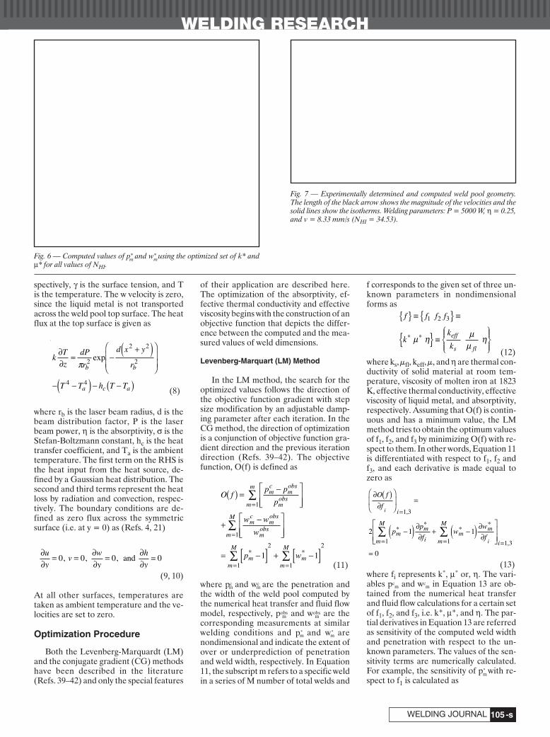
Fig. 6 — Computed values of p* and w* using the optimized set of k* andm* for all values of NHI.

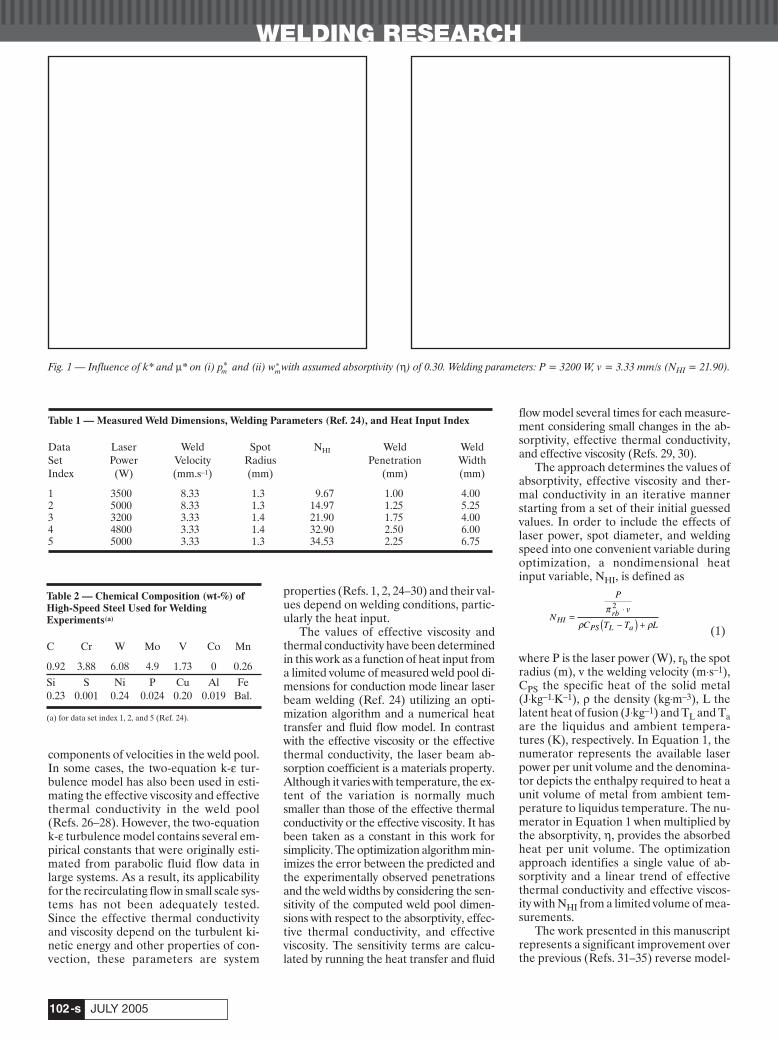
Fig. 7 — Experimentally determined and computed weld pool geometry.The length of the black arrow shows the magnitude of the velocities and thesolid lines show the isotherms. Welding parameters: P = 5000 W, h = 0.25,and v = 8.33 mm/s (NHI = 34.53).

m m

m m

m m

m m

m

De---7_05 6/6/05 4:07 PM Page 105

WELDING RESEARCH

JULY 2005-s106

(14)where df1 is very small compared with f1.The solution of Equation 13 is achievedwhen both p* and w* becomes close to one.In other words, the calculated values of pc

and wc should be close to the correspond-ing measured values of pobs and wobs for allM welds. Since f1, f2, and f3 do not explic-itly appear in Equation 13, this equationneeds to be rearranged so that it can serveas a basis for an iterative scheme to evalu-ate the optimum values of f1, f2, and f3.The procedure is explained in Appendix 1.The final form of equations to be solved is

(15)where,

(16)and {fk+1} refers to the three unknown in-crements after (k+1)th iteration. Equa-tion 15 provides the solution of the threeunknown increments, {Dfk} correspond-ing to the three unknown parameters.

Conjugate Gradient (CG) Method

In the conjugate gradient technique,the unknown parameters are iterativelysearched in the following sequence (Refs.40–42):

(17)where fk+1 represents the values of thethree unknowns after (k+1)th iteration,

indicates the direc-tions of search at theend of kth iterationcorresponding to theunknowns f1, f2, and f3,and ßk is the size of thesearch step. Both dk

and ßk are calculatedfor every iteration orstep. The variable ßk

tends to adjust the ex-tent of increment inunknown parametersbetween successive it-erations and logicallyshould assume a valuethat will facilitate thecondition of objectivefunction minimum.Thus, ßk is calculatedby minimizing theresidual objectivefunction O(fi)k+1

(18)The directions of search, dk , dk, and dk , atthe end of kth iteration are calculated as alinear conjugation of the correspondingdirections of search at the end of (k–1)th

iteration and the respective residual gra-dient of the objective function, O(f), afterkth iteration as

(19)where gk is a conjugation coefficient at theend of kth iteration. The coefficient gk is

obtained either by Equation 20a usingPolok-Ribier’s (CGPR) modification orby Equation 20b using Fletcher-Reeve’smodification (CGFR)

(20a)

(20b)

g

g

kik

ik

ik

i

ik

i

O f O f O f

O f

k

=— ( ){ } — ( ) - — ( ){ }

— ( ){ }= =

-

=

-

=

Â

Â

1

1

3

12

1

3

01 2 0for and , ,...

g

g

kik

i

ik

i

O f

O f

k

=— ( ){ }— ( ){ }

= =

=

-

=

Â

Â

2

1

3

12

1

3

01 2 0

for and , ,...d O f d

d O f d

d O f d

k k k k

k k k k

k k k k

1 1 11

2 2 21

3 3 31

= — ( ) += — ( ) += — ( ) +

-

-

-

g

g

g

∂ ( )∂

= ≥+

O fik

kk

1

0 0b

b ;

f f d iik

ik k

ik+ = -1 b for = 1,3

f f f iik

ik

ik+{ } = { }+ { }1 D for = 1,3

S f Sk[ ]{ } = -{ }*D

∂∂

-

=+Ê

ËÁˆ¯

ÊËÁ

ˆ¯

*

*

*

pf

pf f f f

pf f f

f

m

m

m

1

1 1 2 3

1 2 3

1

d

d

, , ,

, , ,

other known parameters

other known parameters

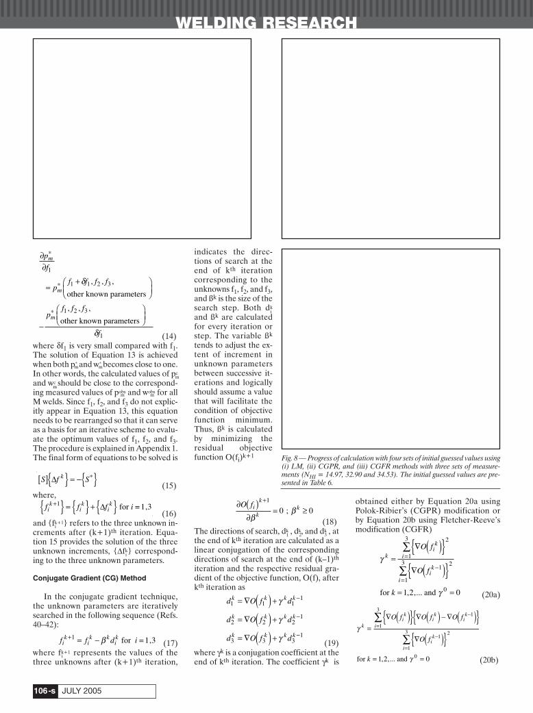
Fig. 8 — Progress of calculation with four sets of initial guessed values using(i) LM, (ii) CGPR, and (iii) CGFR methods with three sets of measure-ments (NHI = 14.97, 32.90 and 34.53). The initial guessed values are pre-sented in Table 6.

m

m

m

m m

m

i

i

i

i

1 2 3

De---7_05 6/6/05 4:08 PM Page 106

WELDING RESEARCH


Further details of these two ap-proaches are given in Appendix 2. In theCG methods, the direction of search is im-portant, since the solution may diverge ifthe direction of search loses sight of theoptimal solution. In the LM method, amanual damping factor is used that con-tinually tracks the search step (or incre-ment) so that the optimal solution cannotmove away from the last computed mini-mum value of the objective function.

There are two main limitations in find-ing property data by the coupled heat andfluid flow and optimization procedure de-scribed in this manuscript. They are 1) theaccuracy of measured depth and widthand 2) how strongly the depth and thewidth vary with the uncertain parameter(sensitivity).

Results and Discussion

The sensitivity of the computed weldpool dimensions with respect to the effec-tive thermal conductivity, effective viscos-ity, and absorptivity were determined byseveral heat transfer and fluid flow calcu-lations. Figures 1A and B depict a numberof isocontours of the dimensionless pene-tration, p* , and the dimensionless width,w* , as a function of k* and m* for data setNo. 3 in Table 1. It is observed from Fig.1A that the dimensionless penetration, p*

increases with k* or m*. However, the di-mensionless width, w* , decreases with k*

or m* as shown in Fig. 1B. For k* valuesabove 7.0, both p* and w* become fairly in-sensitive to m*. Furthermore, both p*

m andw* approached a value of unity at high val-ues of k* and m*. When both p* and w* are1, pc equals pobs and wc equals wobs and thecalculated results agree with the corre-

sponding measured values. The effects of k* and m* on the com-

puted weld pool dimensions can be ex-plained as follows:

The dimensionless weld penetration,p* , increases with k* since high values ofthermal conductivity facilitate rapid heattransport in the downward direction.However, the higher thermal conductivityalso reduces the surface temperature gra-dient and the radial convective heat trans-port and, consequently, decreases. Highervalues of m* lowers radial convection andthe convective heat flow resulting in bothlower weld width and slightly higher peaktemperature. The higher peak tempera-ture enhances downward heat conductionand increases penetration. Furthermore,as k* is progressively increased, conduc-tion becomes the dominant mechanism ofheat transfer and changes in m* do not sig-nificantly alter either the peak tempera-ture or the convective heat transfer rate.Thus, the weld pool dimensions do notchange significantly with m* at high valuesof k* as observed in Fig. 1A and B.

It is quite apparent that in addition tothe variation in k* or m*, any change in thevalue of absorptivity will further influencethe results presented in Fig. 1A and B. Al-though it has been reported that h de-pends on laser power (Ref. 43), the ab-sorptivity is a material property, and itsexact value depends on factors such as thesurface temperature. An increase in thevalue of absorptivity implies an enhance-ment in the heat absorption rate that leadsto higher peak temperature, greater tem-perature gradient and larger computedweld pool dimensions for a specific set ofk* and m*. In contrast, a decrease in thevalue of absorptivity leads to smaller val-ues of computed weld pool dimensions fora specific set of k* and m*. Such a behaviorwas also demonstrated in the case of aGTA weld pool (Ref. 29). To keep theproblem tractable, a single optimizedvalue of absorptivity (h) for all the weld-ing conditions considered in the presentwork is assumed.

Figure 2 shows that high values of k*

and m* are necessary to achieve goodagreement between the computed and theexperimental weld pool geometry, i.e., lowvalues of objective function for data setNo. 3 in Table 1. In contrast, Fig. 3 indi-cates that low values of both k* and m* arenecessary to reduce the objective function

for data set No. 2 in Table 1. These appar-ently contrasting results are achieved forwelds with different heat input indexes(NHI) of 21.90 and 14.97 for data set Nos.3 and 2, respectively. The results in Figs. 2and 3 are consistent with the fact that k*

and m* are not materials properties andtheir optimum values depend on NHI. Toaccount for the same in the procedure ofoptimization of k* and m* in a simplifiedmanner, the following linear relationshipsare assumed for simplicity:

(21)

where C1 and C3 are the minimum valuesof the effective conductivity and effectiveviscosity, respectively, and C2, and C4 areconstants. Since k* and m* equal 1 at lowvalues of NHI, the values of both C1 and C3are taken to be one. Thus, the optimiza-tion routine is used to estimate the valuesof C2 and C4 for each NHI.

Results in Figs. 2 and 3 also indicatethat several combinations of k* and m* mayresult in low values of O(f) for a given NHI.In order to seek optimum values for k* andm* for a particular NHI, an additional con-straint is useful to achieve a physically re-alistic solution. Since k* and m* are relatedby the turbulent Prandtl number, PrT, itsvalue (= 0.9) provides a useful constraint.In other words, out of many possible solu-tions, the specific combination of k* andm* nearest to the line corresponding to PrT= 0.9 will be chosen as the final solution.PrT is defined as

(22)

where meff = mL + mT, keff = kL+ kT and mT,kT are the turbulent viscosity and thermalconductivity, respectively, and mL and kLare the viscosity and thermal conductivityof the liquid, respectively. Finally, Equa-tion 12 is modified as

(23)

A set of initial values of C2, C4 and h isnecessary to start the optimization calcu-lations by all three methods indicated inAppendixes 1 and 2. It is apparent from

f f f f C C{ } ∫ { } ∫ { }1 2 3 2 4 h

PrTT PL

T

C

k= m

k C C N

C C N

HI

HI

* = +

= +1 2

3 4

m *

Table 6 — Sets of Initial Guesses for the Unknown parameters, C2 and C4

Set 1 Set 2 Set 3 Set 4 Optimized values

C2 = 0.5 C2 = 1.0 C2 = 1.5 C2 = 2.0 C2 = 0.252C4 = 0.5 C4 = 1.0 C2 = 1.5 C4 = 2.0 C4 = 1.115h = 0.1 h = 0.2 h = 0.3 h = 0.4 h = 0.250

Table 5 — Data Used for Calculations ofTemperature and Velocity Fields(a)

Physical Property Value

Liquidus temperature, TL (K) 1800.0Solidus temperature, TS (K) 1760.0Ambient temperature, Ta (K) 293.0Density of liquid metal, r (kg/m3) 7.2 ¥ 103

Thermal conductivity of solid, 25.08ks (W m–1 K–1)Thermal conductivity of liquid, 25.08kL (W m–1 K–1)Specific heat of solid, 754.0CPS (J kg–1 K–1)Specific heat of liquid, 754.0CPL (J kg–1 K–1)Temperature coefficient of –0.5 ¥ 10–3

surface tension, dg/dT (N m–1 K–1)Coefficient of thermal 1.5 ¥ 10–6

expansion, b (K–1)Viscosity of molten iron 6.7 ¥ 10–3

at 1823 K, m fl (kg.m–1s–1)

(a) for data set index 3 and 4 (Ref. 24).

m

m

m,

m

m

m

m

m

m m m m

m

m

De---7_05 6/6/05 4:08 PM Page 107

WELDING RESEARCH

JULY 2005-s108

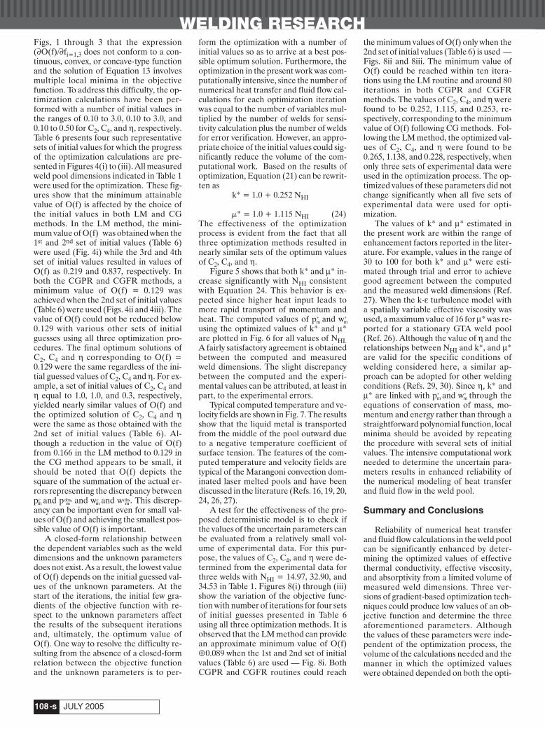
Figs, 1 through 3 that the expression(∂O(f)/∂fi=1,3 does not conform to a con-tinuous, convex, or concave-type functionand the solution of Equation 13 involvesmultiple local minima in the objectivefunction. To address this difficulty, the op-timization calculations have been per-formed with a number of initial values inthe ranges of 0.10 to 3.0, 0.10 to 3.0, and0.10 to 0.50 for C2, C4, and h, respectively.Table 6 presents four such representativesets of initial values for which the progressof the optimization calculations are pre-sented in Figures 4(i) to (iii). All measuredweld pool dimensions indicated in Table 1were used for the optimization. These fig-ures show that the minimum attainablevalue of O(f) is affected by the choice ofthe initial values in both LM and CGmethods. In the LM method, the mini-mum value of O(f) was obtained when the1st and 2nd set of initial values (Table 6)were used (Fig. 4i) while the 3rd and 4thset of initial values resulted in values ofO(f) as 0.219 and 0.837, respectively. Inboth the CGPR and CGFR methods, aminimum value of O(f) = 0.129 wasachieved when the 2nd set of initial values(Table 6) were used (Figs. 4ii and 4iii). Thevalue of O(f) could not be reduced below0.129 with various other sets of initialguesses using all three optimization pro-cedures. The final optimum solutions ofC2, C4 and h corresponding to O(f) =0.129 were the same regardless of the ini-tial guessed values of C2, C4 and h. For ex-ample, a set of initial values of C2, C4 andh equal to 1.0, 1.0, and 0.3, respectively,yielded nearly similar values of O(f) andthe optimized solution of C2, C4 and hwere the same as those obtained with the2nd set of initial values (Table 6). Al-though a reduction in the value of O(f)from 0.166 in the LM method to 0.129 inthe CG method appears to be small, itshould be noted that O(f) depicts thesquare of the summation of the actual er-rors representing the discrepancy betweenpc and pobs, and wc and wobs. This discrep-ancy can be important even for small val-ues of O(f) and achieving the smallest pos-sible value of O(f) is important.

A closed-form relationship betweenthe dependent variables such as the welddimensions and the unknown parametersdoes not exist. As a result, the lowest valueof O(f) depends on the initial guessed val-ues of the unknown parameters. At thestart of the iterations, the initial few gra-dients of the objective function with re-spect to the unknown parameters affectthe results of the subsequent iterationsand, ultimately, the optimum value ofO(f). One way to resolve the difficulty re-sulting from the absence of a closed-formrelation between the objective functionand the unknown parameters is to per-

form the optimization with a number ofinitial values so as to arrive at a best pos-sible optimum solution. Furthermore, theoptimization in the present work was com-putationally intensive, since the number ofnumerical heat transfer and fluid flow cal-culations for each optimization iterationwas equal to the number of variables mul-tiplied by the number of welds for sensi-tivity calculation plus the number of weldsfor error verification. However, an appro-priate choice of the initial values could sig-nificantly reduce the volume of the com-putational work. Based on the results ofoptimization, Equation (21) can be rewrit-ten as

k* = 1.0 + 0.252 NHI

µ* = 1.0 + 1.115 NHI (24)The effectiveness of the optimizationprocess is evident from the fact that allthree optimization methods resulted innearly similar sets of the optimum valuesof C2, C4, and h.

Figure 5 shows that both k* and m* in-crease significantly with NHI consistentwith Equation 24. This behavior is ex-pected since higher heat input leads tomore rapid transport of momentum andheat. The computed values of p* and w*

using the optimized values of k* and m*are plotted in Fig. 6 for all values of NHI.A fairly satisfactory agreement is obtainedbetween the computed and measuredweld dimensions. The slight discrepancybetween the computed and the experi-mental values can be attributed, at least inpart, to the experimental errors.

Typical computed temperature and ve-locity fields are shown in Fig. 7. The resultsshow that the liquid metal is transportedfrom the middle of the pool outward dueto a negative temperature coefficient ofsurface tension. The features of the com-puted temperature and velocity fields aretypical of the Marangoni convection dom-inated laser melted pools and have beendiscussed in the literature (Refs. 16, 19, 20,24, 26, 27).

A test for the effectiveness of the pro-posed deterministic model is to check ifthe values of the uncertain parameters canbe evaluated from a relatively small vol-ume of experimental data. For this pur-pose, the values of C2, C4, and h were de-termined from the experimental data forthree welds with NHI = 14.97, 32.90, and34.53 in Table 1. Figures 8(i) through (iii)show the variation of the objective func-tion with number of iterations for four setsof initial guesses presented in Table 6using all three optimization methods. It isobserved that the LM method can providean approximate minimum value of O(f)≈0.089 when the 1st and 2nd set of initialvalues (Table 6) are used — Fig. 8i. BothCGPR and CGFR routines could reach

the minimum values of O(f) only when the2nd set of initial values (Table 6) is used —Figs. 8ii and 8iii. The minimum value ofO(f) could be reached within ten itera-tions using the LM routine and around 80iterations in both CGPR and CGFRmethods. The values of C2, C4, and h werefound to be 0.252, 1.115, and 0.253, re-spectively, corresponding to the minimumvalue of O(f) following CG methods. Fol-lowing the LM method, the optimized val-ues of C2, C4, and h were found to be0.265, 1.138, and 0.228, respectively, whenonly three sets of experimental data wereused in the optimization process. The op-timized values of these parameters did notchange significantly when all five sets ofexperimental data were used for opti-mization.

The values of k* and m* estimated inthe present work are within the range ofenhancement factors reported in the liter-ature. For example, values in the range of30 to 100 for both k* and m* were esti-mated through trial and error to achievegood agreement between the computedand the measured weld dimensions (Ref.27). When the k-e turbulence model witha spatially variable effective viscosity wasused, a maximum value of 16 for m* was re-ported for a stationary GTA weld pool(Ref. 26). Although the value of h and therelationships between NHI and k*, and m*are valid for the specific conditions ofwelding considered here, a similar ap-proach can be adopted for other weldingconditions (Refs. 29, 30). Since h, k* andm* are linked with p* and w* through theequations of conservation of mass, mo-mentum and energy rather than through astraightforward polynomial function, localminima should be avoided by repeatingthe procedure with several sets of initialvalues. The intensive computational workneeded to determine the uncertain para-meters results in enhanced reliability ofthe numerical modeling of heat transferand fluid flow in the weld pool.

Summary and Conclusions

Reliability of numerical heat transferand fluid flow calculations in the weld poolcan be significantly enhanced by deter-mining the optimized values of effectivethermal conductivity, effective viscosity,and absorptivity from a limited volume ofmeasured weld dimensions. Three ver-sions of gradient-based optimization tech-niques could produce low values of an ob-jective function and determine the threeaforementioned parameters. Althoughthe values of these parameters were inde-pendent of the optimization process, thevolume of the calculations needed and themanner in which the optimized valueswere obtained depended on both the opti-

m m m m

m m

m m

De---7_05 6/6/05 4:08 PM Page 108

WELDING RESEARCH


mization method selected and the initialguessed values of the parameters. The val-ues of effective thermal conductivity andeffective viscosity were found to be muchhigher than their corresponding molecu-lar values and also depended on heatinput. Correlations are proposed to deter-mine these parameters from welding con-ditions. The use of the optimized values ofabsorptivity, effective thermal conductiv-ity and effective viscosity, determinedfrom a limited volume of experimentaldata and the proposed model, resulted ingood agreement between the computedand the experimentally determined fusionzone geometry without the need to adjustthese parameters by trial and error.

AcknowledgmentsThe work was supported by a grant

from the U.S. Department of Energy, Of-fice of Basic Energy Sciences, Division ofMaterials Sciences, under grant numberDE-FGO2-01ER45900. The authors ap-preciate critical comments on the workfrom Mr. S. Mishra, Ms. Xiuli He and Mr.A. Kumar.

References

1. David, S. A., and DebRoy, T. 1992. Cur-rent issues and problems in welding science.Science 257: 497–502.

2. DebRoy, T., and David, S. A. 1995. Phys-ical processes in fusion welding. Rev. Mod. Phys.67(1): 85–112.

3. Zhao, H., White, D. R., and DebRoy, T.1999. Current issues and problems in laserwelding of aluminum alloys. Int. Mater. Rev. 44:238–266.

4. Mundra, K., DebRoy, T., and Kelkar, K.M. 1996. Numerical prediction of fluid flow andheat transfer in welding with a moving heatsource. Numer. Heat Transfer A 29: 115–129.

5. Elmer, J. W., Palmer T. A., Zhang W.,Wood, B., and DebRoy, T. 2003. Kinetic mod-eling of phase transformations occurring in theHAZ of C-Mn steel welds based on direct ob-servations. Acta Materialia. 51(12): 3333–3349.

6. Kou, S., and Wang, Y. H. 1986. Three di-mensional convection in laser melted pools.Metallurgical Transactions A. 17A(12):2265–2270.

7. Pitscheneder, W., DebRoy, T., Mundra,K., and Ebner, R. 1996. Role of sulfur and pro-cessing variables on the temporal evolution ofweld pool geometry during multi-kilowatt laserwelding of steels. Welding Journal 75(3): 71-s to80-s.

8. Cool, T., and Bhadeshia, H. K. D. H. 1997.Austenite formation in 9Cr1Mo type powerplant steels. Sci. Technol. Weld. Joining. 2(1):36–42.

9. Mishra, S., and DebRoy, T. 2004. Graintopology in Ti-6Al-4V welds — Monte Carlosimulation and experiments. Journal of PhysicsD: Applied Physics. 37: 2191–2196.

10. Mishra, S., and DebRoy, T. 2004. Mea-surements and Monte Carlo simulation of grainstructure in the heat-affected zone of Ti-6Al-4V welds. Acta Materialia. 52(5): 1183–1192.

11. Yang, Z. and DebRoy, T. 1999. Model-ing of macro- and microstructures of gas metal

arc welded HSLA-100 steel. Metall. Mater.Trans. B. 30B: 483–493.

12. Hong, T., Pitscheneder, W., and De-bRoy, T. 1998. Quantitative modeling of inclu-sion growth in the weld pool by consideringtheir motion and temperature gyrations. Sci.Technol. Weld. Joining. 3(1): 33–41.

13. Hong, T., and DebRoy, T. 2003. Non-isothermal growth and dissolution of inclusionsin liquid steels. Metal. Mater. Trans. B. 34B:267–269.

14. Hong, T., and DebRoy, T. 2001. Effectsof time, temperature and steel composition onthe growth and dissolution of inclusions in liq-uid steels. Ironmaking and Steelmaking. 28(6):450–454.

15. He, X., Fuerschbach, P., and DebRoy, T.2004. Composition change of stainless steelduring micro-joining with short laser pulse. J.Appl. Phys. (In press).

16. Zhao, H., and DebRoy, T. 2001. Weldmetal composition change during conductionmodel laser welding of 5182 aluminum alloy.Metall. Mater. Trans. B. 32B: 163–172.

17. Palmer, T. A., and DebRoy, T. 2000. Nu-merical modelling of enhanced nitrogen disso-lution during GTA welding. Metall. Mater.Trans. B. 31B(6): 1371–1385.

18. Mundra, K., Blackburn, J. M., and De-bRoy, T. 1997. Absorption and transport of hy-drogen during GMA welding of mild steels. Sci.Technol. Weld. Joining. 2(4): 174–184.

19. He, X., Fuerschbach, P. W., and DebRoy,T. 2003. Heat transfer and fluid flow duringlaser spot welding of 304 stainless steel. J. Phys.D: Appl. Phys. 36(12): 1388–1398.

20. Zhao, H. and DebRoy, T. 2003. Macro-porosity free aluminum alloy weldmentsthrough numerical simulation of keyhole modelaser welding. J. Appl. Phys. 93(12):10089–10096.

21. Zhang, W., Roy, G. G., Elmer, J. W,. andDebRoy, T. 2003. Modeling of heat transfer andfluid flow during gas tungsten arc spot weldingof low carbon steel. J. Appl. Phys. 93(5):3022–3033.

22. Kumar, A., and DebRoy, T. 2003. Calcu-lation of three-dimensional electromagneticforce field during arc welding. J. Appl. Phys.94(2): 1267–1277.

23. Kim, C. H., Zhang, W. and DebRoy, T.2003. Modeling of temperature field and solid-ified surface profile during gas metal arc filletwelding. J. Appl. Phys. 94(4): 2667–2679.

24. Pitscheneder, W. 2001. Contribution tothe understanding and optimization of lasersurface alloying. PhD Dissertation. Universityof Leoben, Austria.

25. DebRoy, T., Mazumdar, A. K., andSpalding, D. B. 1978. Numerical prediction ofrecirculating flows with free convection en-countered in gas-stirred reactors. Applied Math-ematical Modelling. 2: 146–150.

26. Hong, K., Weckmann, D. C., Strong, A.B., and Zheng, W. 2002. Modelling turbulentthermofluid flow in stationary gas tungsten arcwelded pools. Sci. Technol. Weld. Joining. 7(3):125–136.

27. Choo, R. T. C., and Szekely, J. 1994. Thepossible role of turbulence in GTA weld poolbehavior. Welding Journal 73(2): 25-s to 31-s.

28. Jonsson, P. G., Szekely, J., Choo, R. T. C.,and Quinn, T. P. 1994. Mathematical models oftransport phenomena associated with arc weld-ing processes: a survey. Modelling Simul. Mater.Sci. Eng. 2(5): 995–1016.

29. De, A., and DebRoy, T. 2004. Probing

unknown welding parameters from convectiveheat transfer calculation and multivariate opti-mization. J. Phys. D: Appl. Phys. 37(1): 140–150.

30. De, A., and DebRoy, T. 2004. A smartmodel to estimate effective thermal conductiv-ity and viscosity in weld pool. Journal of AppliedPhysics. 95(9): 5230–5240.

31. Hsu, Y. F., Rubinsky, B. and Mahin, K.1986. An inverse finite element method for theanalysis of stationary arc welding process. J.Heat Transfer, Trans. ASME. 108(4): 734–741.

32. Beck, J. V. 1991. Inverse problems inheat transfer with application to solidificationand welding. Proc. 5th Int. Conf. on Modeling ofCasting, Welding and Advanced SolidificationProcesses, eds. M. Rappaz et al., pp. 503–514.The Minerals, Metals and Materials Society,Warrendale, Pa.

33. Rappaz, M., Desbiolles, J. L., Drezet, J.M., Gandin, C. A., Jacot, A., and Thevoz, P.1995. Proc. 7th Int. Conf. on Modeling of Cast-ing, Welding and Advanced SolidificationProcesses, eds. M. Cross et al., pp. 449–457, TheMinerals, Metals and Materials Society, War-rendale, Pa.

34. Fonda, R. W. and Lambrakos, S. G.2002. Analysis of friction stir welds using an in-verse problem approach. Sci. Technol. Weld.Joining 7(3): 177–181.

35. Karkhin, V. A., Plochikhine, V. V., andBergmann, H. W. 2002. Solution of inverse heatconduction problem for determining heatinput, weld shape, and grain structure duringlaser welding. Sci. Technol. Weld. Joining 7(4):224–231.

36. Patankar, S. V. 1992. Numerical HeatTransfer and Fluid Flow. New York, McGraw-Hill.

37. Voller, V. R., and Prakash, C. 1987. Afixed grid numerical modeling methodology forconvection-diffusion mushy region phasechange problems. Int. J. Heat Mass Transf. 30:1709–1719.

38. Brent, A. D., Voller, V. R., and Reid, K.J. 1988. The enthalpy porosity technique formodeling convection-diffusion phase change:application to the melting of a pure metal. Nu-merical Heat Transfer 13: 297–318.

39. Beck, J. V., and Arnold, K. J. 1977. Pa-rameter Estimation in Engineering and Science.New York, N.Y., Wiley International.

40. Beck, J. V., Blackwell, B., and Clair, C.R., Jr. 1985. Inverse Heat Conduction—Ill PosedProblems. New York, N.Y., Wiley International.

41. Alifanov, O. M. 1994. Inverse heat Trans-fer Problems. Berlin, Springer-Verlag.

42. Ozisik, M. N., and Orlande, H. R. B.2000. Inverse Heat Transfer. 35, New York, N.Y.,Taylor & Francis Inc.

43. Fuerschbach, P. W. 1996. Measurementand prediction of energy transfer efficiency inlaser beam welding. Welding Journal 75(1): 24-sto 34-s.

Appendix 1

In order to explain the basic concept ofthe LM method, a simplified system in-volving three unknown parameters, f1, f2,and f3, and one dependent variable, p*

m

measured under five welding conditions isconsidered first. Equation 13 can be writ-ten for f1, f2, and f3 as:

De---7_05 6/6/05 4:08 PM Page 109

WELDING RESEARCH

JULY 2005-s110

(A1, A2, A3)

The values of the three unknowns, f1, f2,and f3 cannot be directly obtained fromthe above equations since they do not ap-pear explicitly in these equations. Thesymbols f1, f2, and f3 resemble k*, m*, andh (absorptivity), respectively. So, the de-pendent variable p* is expanded using theTaylor’s series expansion to explicitly con-tain values of increments and, f1, f2, and f3.Considering two successive iterations ofp*

m and taking only the first order terms

(A4)

where Dfk, Dfk and Dfk are three unknownincrements corresponding to f1, f2, and f3as

(A5)

and fk+1, fk+1, and fk+1 correspond to thevalues of three unknowns after (k+1)th it-eration. Except Dfk, Dfk, and Dfk, all otherterms on the right hand side of EquationA4 are considered to be known. To solvefor Dfk, Dfk, and Dfk, Equations A1, A2 andA3 are first rewritten replacing p* by(p*)k+1 as

(A6, A7, A8)However, p* equals to pc /pobs, and al-though pobs is a known measured value, pc

is to be computed using the numericalheat transfer and fluid flow calculation for

a set of f1, f2, f3 and other known parame-ters. So, (p* )k+1 that is the value of p* after(k+1)th iteration is unknown since Dfk,Dfk,and Dfk are unknown. Next, substitut-ing right hand side of Equation A4 in theplace of (p* )k+1, Equations A6, A7, and A8are rewritten as:

(A9)

(A10)

(A11)

Neglecting higher order differentials e.g

etc., Equations A9, A10

and A11 are further simplified as:

(A12)

(A13)

(A14)Equations A12, A13, and A14 are next re-arranged as

(A15)

∂( )∂

∂( )∂

È

Î

ÍÍÍ

˘

˚

˙˙˙

+

∂( )∂

∂( )∂

È

Î

ÍÍÍ

˘

˚

˙˙˙

+

∂( )∂

∂( )∂

È

Î

ÍÍÍ

˘

˚

˙˙˙

* *

=

* *

=

* *

=

Â

Â

Â

p

f

p

ff

p

f

p

ff

p

f

p

ff

mk

mk

m

k

mk

mk

m

k

mk

mk

m

1 11

5

1

1 21

5

2

1 31

5

D

D

D 33

11

51

k

mk

mk

m

p

fp

=

-∂( )

∂ ( ) -ÊË

ˆ¯

È

Î

ÍÍÍ

˘

˚

˙˙˙

**

=Â

pp

ff

p

ff

p

ff

p

f

mk m

k

k

mk

k

mk

k

mk

**

*

*

*

( ) +∂( )

∂+

∂( )∂

+

∂( )∂

-

Ê

Ë

ÁÁÁÁÁÁÁÁÁÁÁÁ

ˆ

¯

˜˜˜˜˜˜˜˜˜˜˜˜

∂( )∂

È

Î

ÍÍÍÍÍÍÍÍÍÍÍÍÍ

˘

˚

˙˙˙˙˙˙˙˙˙

11

22

33

3

1

D

D

D˙˙˙˙

==

Âm 1

50

pp

ff

p

ff

p

ff

p

f

mk m

k

k

mk

k

mk

k

mk

**

*

*

*

( ) +∂( )

∂+

∂( )∂

+

∂( )∂

-

Ê

Ë


ˆ

¯

˜˜˜˜˜˜˜˜˜˜˜˜

∂( )∂

È

Î


˘

˚

˙˙˙˙˙˙˙˙˙

11

22

33

2

1

D

D

D˙˙˙˙

==

Âm 1

50

pp

ff

p

ff

p

ff

p

f

mk m

k

k

mk

k

mk

k

mk

**

*

*

*

( ) +∂( )

∂+

∂( )∂

+

∂( )∂

-

Ê

Ë


ˆ

¯

˜˜˜˜˜˜˜˜˜˜˜˜

∂( )∂

È

Î


˘

˚

˙˙˙˙˙˙˙˙˙

11

22

33

1

1

D

D

D˙˙˙˙

==

Âm 1

50

∂∂

∂( )∂

Ê

ËÁÁ

ˆ

¯˜˜

*

f

p

ff

m k

1 11D

pp

ff

p

ff

p

ff

pp

ff

p

ff

p

f

mk m

k

k

mk

k mk

k

mk m

k

k

mk

k mk

**

* *

**

* *

( ) +∂( )

∂+

∂( )∂

+∂( )

∂-

Ê

Ë

ÁÁÁÁÁÁ

ˆ

¯

˜˜˜˜˜˜

∂( ) +

∂( )∂

+

∂( )∂

+∂( )

∂

11

22

33

11

22

3

1

D

D D

D

D DDf

f

k

m

3

3

1

50Ê

Ë

ÁÁÁÁÁÁ

ˆ

¯

˜˜˜˜˜˜

∂

È

Î

ÍÍÍÍÍÍÍÍÍÍÍÍÍÍÍÍÍ

˘

˚

˙˙˙˙˙˙˙˙˙˙˙˙˙˙˙˙˙

==

Â

pp

ff

p

ff

p

ff

pp

ff

p

ff

p

f

mk m

k

k

mk

k mk

k

m

k mk

k

mk

k mk

**

* *

*

*

* *

( ) +∂( )

∂+

∂( )∂

+∂( )

∂-

Ê

Ë

ÁÁÁÁÁÁ

ˆ

¯

˜˜˜˜˜˜

∂( ) +

∂( )∂

+

∂( )∂

+∂( )

∂

11

22

33

11

22

3

1

D

D D

D

D DDf

f

k

m

3

2

1

50Ê

Ë

ÁÁÁÁÁÁ

ˆ

¯

˜˜˜˜˜˜

∂

È

Î


˘

˚

˙˙˙˙˙˙˙˙˙˙˙˙˙˙˙˙˙

==

Â

pp

ff

p

ff

p

ff

pp

ff

p

ff

p

f

mk m

k

k

mk

k mk

k

m

k mk

k

mk

k mk

**

* *

*

*

* *

( ) +∂( )

∂+

∂( )∂

+∂( )

∂-

Ê

Ë

ÁÁÁÁÁÁ

ˆ

¯

˜˜˜˜˜˜

∂( ) +

∂( )∂

+

∂( )∂

+∂( )

∂

11

22

33

11

22

3

1

D

D D

D

D DDf

f

k

m

3

1

1

50Ê

Ë

ÁÁÁÁÁÁ

ˆ

¯

˜˜˜˜˜˜

∂

È

Î


˘

˚

˙˙˙˙˙˙˙˙˙˙˙˙˙˙˙˙˙

==

Â

pp

f

pp

f

pp

f

m

k m

k

m

m

k m

k

m

m

k m

k

* +* +

=

* +* +

=

* +* +

( ) -ÊË

ˆ¯

∂( )∂

È

Î

ÍÍÍ

˘

˚

˙˙˙

=

( ) -ÊË

ˆ¯

∂( )∂

È

Î

ÍÍÍ

˘

˚

˙˙˙

=

( ) -ÊË

ˆ¯

∂( )∂

È

Î

ÍÍ

Â

Â

11

11

5

11

21

5

11

3

1 0

1 0

1

;

ÍÍ

˘

˚

˙˙˙

==

Âm 1

5

0

f f f

f f f

f f f

k k k

k k k

k k k

11

1 1

21

2 2

31

3 3

+

+

+

= +

= +

= +

D

D

D

p pp

ff

p

ff

p

ff

m

k

m

k m

k

k

m

k

k m

k

k

* + **

* *

( ) = ( ) +∂( )

∂+

∂( )∂

+∂( )

∂

1

11

2 32 3

D

D D

pp

f

pp

f

pp

f

mm

m

mm

m

mm

m

**

=

**

=

**

=

-( ) ∂∂

È

ÎÍÍ

˘

˚˙˙

=

-( ) ∂∂

È

ÎÍÍ

˘

˚˙˙

=

-( ) ∂∂

È

ÎÍÍ

˘

˚˙˙

=

Â

Â

Â

1 0

1 0

1 0

11

5

21

5

31

5

;

;

m m

m mm

m

1 2 3

1

1 2

2

1 2 3

m

m

3

3

1

m

m m

2 3

De---7_05 6/9/05 3:25 PM Page 110

WELDING RESEARCH


(A16)

(A17)

Equations A15, A16, and A17 can be ex-pressed in matrix form as

[S]{Dfk}=–{S*} (A18)where

(A19)

(A20, A21)

Thus, Equations A1, A2, and A3 are mod-ified to equation A18 where the three un-known incremental terms Dfk, Dfk, and Dfk

are explicitly defined in terms of theknown quantities. The solution of Dfk, Dfk,and Dfk are used next to obtain fk+1 , fk+1,and fk+1 (expression A5) that are em-ployed to compute (pc )k+1 using the nu-merical heat transfer and fluid flow model.Next, O(f)k+1 is calculated as

(A22)

Values of f1, f2, and f3 are assumed to reachoptimum when the calculated value ofO(f)k+1 is smaller than a predefined smallnumber. For the two dependent variablesp* and w* , Equation A19 is modified as

(A23)where

(A24)Equation A20 will be modified as

(A25)

Equations A5 and A21 do not changesince the number of unknown parametersremains three. Furthermore, the sensitiv-ity terms such as

(for i = 1 to 3) inEquation A18 often tend to be very smallas the values of the unknown parametersf1, f2 and f3 move close to the optimum. Asa result, the matrix [S] tends to becomesingular. To avoid numerical instability,Equation A18 is further modified follow-ing the LM method as

(A26)

where l is a scalar damping coefficient,usually about 0.001, and I is a diagonal ma-trix given by (Ref. 42)

(A27)

The product lI in Equation A26 ensuresthat the left-hand term in Equation A26will remain nonzero even if the determi-nant of the matrix [S] is zero. The value ofl is usually increased or decreased by afactor of ten as the value of the objectivefunction in subsequent iterations in-creases or decreases. This, in effect, en-sures the reduction or enhancement instep size as the solution respectively tendsto diverge or converge. The algorithm ofthe complete procedure using the LMmethod can be presented as follows:

Step 1. Guess initial values (e.g., kth) ofunknown variables set, {fk} for i=1, 3 fromEquation 12.

Step 2. Choose initial value of dampingfactor (l).

Step 3. Compute the value of the ob-jective function, O(fk) from Equation 11.

Step 4. Solve for the set of unknown in-

I

S

=È

Î

ÍÍÍ

˘

˚

˙˙˙

11 0 0

0 S 0

0 0 S22

33

S I f Sk[ ] +( ){ } = -{ }*l D

∂( )∂

∂( )∂

* *p

f

w

f

mk

i

mk

i or

S

S

S

S

p

fp

w

fw

p

fp

pw

pw

pw

mk

mk m

mk

m

mk

mk

*

**

**

=

**

{ } =

Ï

ÌÔÔ

ÓÔÔ

¸

˝ÔÔ

˛ÔÔ

=

∂( )∂ ( ) -

ÊËÁ

ˆ¯

+∂( )

∂ ( ) -ÊËÁ

ˆ¯

Ê

Ë

ÁÁÁ

ˆ

¯

˜˜˜

∂( )∂ ( ) -

ÊËÁ

ˆ¯

+

Â

1

2

3

1 11

5

2

1 1

1∂∂( )

∂ ( ) -ÊËÁ

ˆ¯

Ê

Ë

ÁÁÁ

ˆ

¯

˜˜˜

∂( )∂ ( ) -

ÊËÁ

ˆ¯

+∂( )

∂ ( ) -ÊËÁ

ˆ¯

Ê

Ë

ÁÁÁ

ˆ

¯

˜˜˜

Ï

Ì

ÔÔÔÔÔÔÔ

Ó

ÔÔÔÔÔ

**

=

**

**

=

Â

Â

w

fw

p

fp

w

fw

mm

k

m

mk

mk m

mk

m

21

5

3 31

5

1

1 1ÔÔÔ

¸

˝

ÔÔÔÔÔÔÔ

˛

ÔÔÔÔÔÔÔ

S

p

f

p

f

w

f

w

f

i jij

mk

i

mk

j

mk

i

mk

j

m

=

∂( )∂

∂( )∂

+

∂( )∂

∂( )∂

Ê

Ë

ÁÁÁÁÁÁÁ

ˆ

¯

˜˜˜˜˜˜

=

* *

* *=Â

1

51 3 for to ,

S

S S S

S S S

S S

[ ] =È

Î

ÍÍÍ

˘

˚

˙˙˙

11 12 13

21 22 23

31 33

S 32

O f pk

m

k

m( ) = ( ) -Ê

Ëˆ¯

+ * +

=Â1 1

1

5 2

1

and S

S

S

S

p

fp

p

fp

p

fp

p

p

p

mk

mk

m

mk

mk

m

mk

mk

m

*

**

=

**

=

**

=

{ } =

Ï

ÌÔÔ

ÓÔÔ

¸

˝ÔÔ

˛ÔÔ

=

∂( )∂ ( ) -Ê

Ëˆ¯

∂( )∂ ( ) -Ê

Ëˆ¯

∂( )∂ ( ) -Ê

Ëˆ¯

Ï

Ì

ÔÔÔÔ

Â

Â

Â

1

2

3

11

5

21

5

31

5

1

1

1

ÔÔ

Ó

ÔÔÔÔÔ

¸

˝

ÔÔÔÔÔ

˛

ÔÔÔÔÔ

{ } =

Ï

ÌÔÔ

ÓÔÔ

¸

˝ÔÔ

˛ÔÔ

D

D

D

D

f

f

f

f

k

k

k

k

1

2

3

S

S S S

S S S

S S

p

f

p

f

p

f

p

f

p

f

p

f

p

m

k

m

k

m

k

m

k

mm

m

k

m

k

m

m

[ ] =È

Î

ÍÍÍ

˘

˚

˙˙˙

=

∂( )∂

∂( )∂

∂( )∂

∂( )∂

∂( )∂

∂( )∂

∂

* * * *

==

* *

=

*

ÂÂ

Â

11 12 13

21 22 23

31 33

1 1 1 21

5

1

5

1 31

5

S 32

(( )∂

∂( )∂

∂( )∂

∂( )∂

∂( )∂

∂( )∂

∂( )∂

∂( )∂

∂( )∂

∂( )∂

*

=

* * * *

==

* *

=

* *

Â

ÂÂ

Â

k

m

k

m

m

k

m

k

m

k

m

k

mm

m

k

m

k

m

m

k

m

k

f

p

f

p

f

p

f

p

f

p

f

p

f

p

f

p

f

p

f

2 11

5

2 2 2 31

5

1

5

3 11

5

3 2mm

m

k

m

k

m

p

f

p

f

=

* *

=

Â

Â∂( )

∂

∂( )∂

È

Î

ÍÍÍÍÍÍÍÍÍÍÍÍÍÍÍÍÍÍÍÍ

˘

˚

˙˙˙˙˙˙˙˙˙˙˙˙˙˙˙˙˙˙˙˙

1

5

3 31

5

∂( )∂

∂( )∂

È

Î

ÍÍÍ

˘

˚

˙˙˙

+

∂( )∂

∂( )∂

È

Î

ÍÍÍ

˘

˚

˙˙˙

+

∂( )∂

∂( )∂

È

Î

ÍÍÍ

˘

˚

˙˙˙

* *

=

* *

=

* *

=

Â

Â

Â

p

f

p

ff

p

f

p

ff

p

f

p

ff

mk

mk

m

k

mk

mk

m

k

mk

mk

m

3 11

5

1

3 21

5

2

3 31

5

D

D

D 33

31

51

k

mk

mk

m

p

fp

=

-∂( )

∂ ( ) -ÊË

ˆ¯

È

Î

ÍÍÍ

˘

˚

˙˙˙

**

=Â

∂( )∂

∂( )∂

È

Î

ÍÍÍ

˘

˚

˙˙˙

+

∂( )∂

∂( )∂

È

Î

ÍÍÍ

˘

˚

˙˙˙

+

∂( )∂

∂( )∂

È

Î

ÍÍÍ

˘

˚

˙˙˙

* *

=

* *

=

* *

=

Â

Â

Â

p

f

p

ff

p

f

p

ff

p

f

p

ff

mk

mk

m

k

mk

mk

m

k

mk

mk

m

2 11

5

1

2 21

5

2

2 31

5

D

D

D 33

21

51

k

mk

mk

m

p

fp

=

-∂( )

∂ ( ) -ÊË

ˆ¯

È

Î

ÍÍÍ

˘

˚

˙˙˙

**

=Â

1

3

3

1

1 2

2

2

3

m

i

m m

De---7_05 6/6/05 4:08 PM 1

WELDING RESEARCH

JULY 2005-s112

crements {Dfk} for i = 1, 3 from EquationA26.

Step 5. Compute {fk+1} for i = 1, 3 fromEquation A5.

Step 6. Compute O(fk+1) from Equa-tion 11.

Step 7. If O(fk+1) ≥ O(fk), set l = 10 l;reject {fk+1}; go back to step 4.

Step 8. If O(fk+1) < O(fk), set l = 0.1 l.Step 9. Exit if O(fk+1) – O(fk) ≤ e1 and

{fk+1}–{fk} ≤ e2; or go back to step 4. e1

and e2 are two small, predefined numbers.

Appendix 2

Considering the objective function de-fined in Equation 11 with two dependentvariables, p* and w* ,and three unknownparameters, f1, f2, and f3, Equation 17 canbe written as

(A28)where fk+1 , fk+1, dk, dk, and bk confirm totheir definitions presented previously. InEquation 18, as O(fi)k+1 contains (p* )k+1

and (w* )k+1 obtained from numerical heattransfer and fluid flow code using values offk+1 , fk+1, and fk+1, and O(fi)k+1 depends onfk+1 , fk+1, and fk+1. Thus, replacing (fi)k+1 inEquation 18 by fk+1 , fk+1, and fk+1, and sub-stituting the right-hand side of EquationA28 in place of them, Equation 18 can berewritten as

(A29)

Considering two dependent variables,and p*

m , w*m ,

can be ex-pressed further as

(A30)Substituting Equation A30 in EquationA29 and using Taylor’s expansion, Equa-tion A29 can be substantially rearrangedto give bk as (Refs. 41, 42)

(A31)Furthermore, following Equation 13,

Equations 20a and 20b can respectively berewritten as

(A32)

(A33)for k = 1, 2 and, g0 = 0. Apart from the cal-culation of conjugate coefficient, gk, bothCGPR and CGFR methods are the same.

g k

mm

ik m

m

ik

mm

ik

m

ik

mm

ik

m

ik

pp

fw

w

f

pp

f

p

f

ww

f

w

f=

-( ) ∂

∂+ -( ) ∂

∂

ÏÌÔ

ÓÔ

¸˝Ô

Ô

-( ) ∂

∂-

∂

∂

Ê

ËÁÁ

ˆ

¯˜ +

-( ) ∂

∂-

∂

∂

Ê

ËÁÁ

ˆ

¯˜

Ï

Ì

ÔÔ

**

**

** *

-

** *

-

1 1

1

1

1

1

ÔÔ

Ó

ÔÔÔ

¸

˝

ÔÔÔ

˛

ÔÔÔ

È

Î

ÍÍÍÍÍÍÍÍÍÍÍÍ

˘

˚

˙˙˙˙˙˙˙˙˙˙˙˙

-( ) ∂

∂+ -( ) ∂

∂

ÏÌÔ

ÓÔ

¸˝Ô

Ô

==

**

-*

*

-==

ÂÂ

ÂÂ

mi

mm

ik m

m

ik

mi

pp

fw

w

f

1

5

1

3

1 1

2

1

5

1

31 1

g k

mm

ik m

m

ik

mi

mm

ik m

m

ik

mi

pp

fw

w

f

pp

fw

w

f

=

-( ) ∂

∂+ -( ) ∂

∂

ÏÌÔ

ÓÔ

¸˝Ô

Ô

-( ) ∂

∂+ -( ) ∂

∂

ÏÌÔ

ÓÔ

¸˝Ô

Ô

**

**

==

**

-*

*

-==

ÂÂ

ÂÂ

1 1

1 1

2

1

5

1

3

1 1

2

1

5

1

3

b k

pm

pm

f kd k pm

f kd k

pm

f kd k

wm

wm

f kd k wm

f kd k

w

=

* -ÊË

ˆ¯

∂ *

∂+

∂ *

∂

+∂ *

∂

Ê

Ë

ÁÁÁÁÁÁ

ˆ

¯

˜˜˜˜˜˜

È

Î

ÍÍÍÍÍÍÍ

˘

˚

˙˙˙˙˙˙˙

+

* -ÊË

ˆ¯

∂ *

∂+

∂ *

∂

+∂

11

12

2

33

11

12

2

mm

f kd k

m

pm

f kwm

f kd k

*

∂

Ê

Ë

ÁÁÁÁÁÁ

ˆ

¯

˜˜˜˜˜˜

È

Î

ÍÍÍÍÍÍÍ

˘

˚

˙˙˙˙˙˙˙

Ï

Ì

ÔÔÔÔÔÔÔÔ

Ó

ÔÔÔÔÔÔÔÔ

¸

˝

ÔÔÔÔÔÔÔÔ

˛

ÔÔÔÔÔÔÔÔ

=

∂ *

∂+

∂ *

∂

Ê

ËÁÁ

ˆ

¯˜˜

+

∂

Â

33

1

5

1 11

ppm

f kwm

f kd k

pm

f kwm

f kd k

m

*

∂+

∂ *

∂

Ê

ËÁÁ

ˆ

¯˜˜

+

∂ *

∂+

∂ *

∂

Ê

ËÁÁ

ˆ

¯˜˜

È

Î


˘

˚

˙˙˙˙˙˙˙˙˙˙˙˙˙

=Â

2 22

3 33

2

1

5

O f d f d f d

p f d f d f d

w f d f d f d

k k k k k k k k k

mk k k k k k k k k

m

mk k k k k k k k k

1 1 2 2 3 3

1 1 2 2 3 31

5

1 1 2 2 3 3

1

1

- - -( )∫ - - -( ) -È

ÎÍ˘˚

+ - - -( ) -

*

=

*

Â

b b b

b b b

b b b

, ,

, ,

, ,ÈÈÎÍ

˘˚=

Âm 1

5

O f d f d f dk k k k k k k k k1 1 2 2 3 3- - -( )b b b, ,

∂- -

-

Ê

ËÁ

ˆ

¯˜

∂= ≥

Of d f

d f d

k k k k

k k k k k

kk

1 1 2

2 3 3 0 0

b

b bb

b

,

,;

f f d

f f d

f f d

k k k k

k k k k

k k k k

11

1 1

21

2 2

31

3 3

+

+

+

= -

= -

= -

b

b

b

Call For PapersThe 6th European Conference on Welding, Joining, and Cutting

Santiago de Compostela, Spain, June 28–30, 2006

The 6th European Conference on Welding, Joining, and Cutting, sponsored by the European Federation for Joining, Welding, andCutting (EWF), in association with the Spanish Association of Welding and Joining Technologies (CESOL), and the MetallurgicalResearch Association of the Northwest (AIMEN), has issued a call for papers and posters.

Papers are sought on a wide variety of topics including welding, joining, surfacing, cutting and related processes and equipment, suchas laser beam and plasma arc welding, brazing and soldering, adhesive bonding, friction stir welding, resistance welding, welding con-sumables. Visit www.cesol.es/EUROJOIN6/16JTS.php for a complete list of recommended topics, detailed author’s submittal infor-mation, and description of the prizes to be presented in four categories.

The deadline for submission of titles and 300–500-word abstracts is September 30, 2005. The deadline for submission of completedconference papers or posters is February 28, 2006. Manuscripts and oral presentations may be presented in English or Spanish.Documents must be submitted in electronic MS Word format with figures provided in TIFF, JPEG, or GIF formats.

Send your intention to participate, including title and abstract of the work to be presented, to CESOL, Gabino Jimeno 5B, 28026Madrid, Spain; FAX: +34 91 500 53 77; [email protected], by September 30, 2005.

i

i

i

m m

i

1 12 2

m

m

1

1

1

2

2

2

3

3

3

i

De---7_05 6/6/05 4:08 PM Page 112