1

Reliable SPICE Simulations of Memristors,Memcapacitors and Meminductors

Dalibor Biolek, Member, IEEE, Massimiliano Di Ventra and Yuriy V. Pershin, Senior Member, IEEE

Abstract—Memory circuit elements, namely memristive, mem-capacitive and meminductive systems, are gaining considerableattention due to their ubiquity and use in diverse areas of scienceand technology. Their modeling within the most widely usedenvironment, SPICE, is thus critical to make substantial progressin the design and analysis of complex circuits. Here, we presenta collection of models of different memory circuit elements andprovide a methodology for their accurate and reliable modeling inthe SPICE environment. We also provide codes of these modelswritten in the most popular SPICE versions (PSpice, LTspice,HSPICE) for the benefit of the reader. We expect this to be ofgreat value to the growing community of scientists interested inthe wide range of applications of memory circuit elements.

I. INTRODUCTION

There is presently a large interest in what are commonlycalled memristors, memcapacitors and meminductors (or col-lectively simply memelements), namely resistors, capacitorsand inductors with memory, respectively [1]. This class ofcircuit elements offers considerable advantages compared totraditional devices. Specifically, these are two-terminal elec-tronic devices that can store analog information even inthe absence of a power source. From the point of view ofpotential applications, memelements open up the possibilityof manipulating and storing information within a totally dif-ferent computing paradigm [2], [3], [4], [5], [6], [7], extendfunctionality of traditional devices [8], as well as serve asmodel systems for certain biological processes and systems[9], [10], [11], [12].

Mathematically, an nth-order u-controlled memelement isdefined by the equations [1]

y(t) = g (x, u, t)u(t) (1)x = f (x, u, t) . (2)

Here, u(t) and y(t) are any two circuit variables (current,charge, voltage, or flux) denoting input and output of thesystem, x is an n-dimensional vector of internal state vari-ables, g is a generalized response, and f is a continuousn-dimensional vector function. Special interest is devoted todevices determined by three pairs of circuit variables: current-voltage (memristive systems), charge-voltage (memcapacitive

D. Biolek is with the Department of Electrical Engineering/Microelec-tronics, University of Defence/Brno University of Technology, Brno, CzechRepublice-mail: dalibor.biolek@unob.cz

M. Di Ventra is with the Department of Physics, University of California,San Diego, La Jolla, California 92093-0319 USAe-mail: diventra@physics.ucsd.edu.

Y. V. Pershin is with the Department of Physics and Astronomy and USCNanocenter, University of South Carolina, Columbia, SC, 29208 USAe-mail: pershin@physics.sc.edu.

systems), and flux-current (meminductive systems). Two otherpairs (charge-current and voltage-flux) are linked throughequations of electrodynamics and therefore are of no practicalinterest. Devices defined by the relation of charge and flux(the latter being the integral of the voltage) are not consideredas a separate group since such devices can be redefined in thecurrent-voltage basis [13].

However, future progress in the analysis of complex circuitsinvolving any of these elements requires reliable simulationtools that are easy to implement and flexible enough to providesolid predictions on a wide range of physically realizable mod-els. The Simulation Program with Integrated Circuit Emphasis(SPICE) environment is one such general-purpose simulatorthat has been successfully used in the analysis of integratedcircuits for forty years. SPICE allows the testing of complexcircuits before they are actually implemented experimentally,thus saving a lot of time and resources in their fabrication.

Being new on the circuit scene, memelements do not havemany years of testing within the SPICE environment. Nonethe-less, more and more SPICE models are being consideredwith different levels of complexity [14], [15], [16], [17], [18],[19], [20], [21], [22]. Oftentimes, readers are interested inthe SPICE code itself and its reliability within the range ofphysical parameters used. Unfortunately, both the codes andreliability criteria are not always available in the literature thuslimiting the use of some of the most popular SPICE modelsof memelements.

This paper attempts to fill this gap by providing severalmodels of ideal and non-ideal memristive, memcapacitive andmeminductive elements and their implementation (codes) inthe most popular SPICE versions (PSpice, LTspice, HSPICE),focusing on the well-known PSpice. Our goal is also to providea general methodology for accurate modeling within this en-vironment so that readers interested in implementing differentmodels can easily build from the examples we provide inthis paper and venture out on their own. We think this couldalso serve as an excellent teaching tool complementing others(e.g., experiment-based ones [23]) for the next generation ofscientists and engineers interested in this field. This method-ology is given in Section II which follows this Introduction.In later Sections we will then focus on specific examplesof memristive, memcapacitive and meminductive systems andtheir modeling in SPICE.

Importantly, instead of focusing on different levels ofsophistication in describing the same electronic device, weconcentrate on SPICE models of physically different memorydevices (e.g., bipolar, unipolar, etc.) that are generally classi-fied as memristive, memcapacitive or meminductive systems.

arX

iv:1

307.

2717

v1 [

phys

ics.

com

p-ph

] 1

0 Ju

l 201

3

2

For completeness, such a presentation is integrated with mod-els of ideal memory elements – memristors, memcapacitorsand meminductors. For each device, we select a reasonablecomplexity in modeling essential features of device operationrelying, in some cases, on original models proved to be usefulin device simulations.

II. METHODOLOGY FOR ACCURATE AND RELIABLEMODELING OF MEMELEMENTS WITH SPICE

Throughout the development of memelement models andtheir implementation in SPICE-family simulation programs,several limitations and specific features of these programsshould be taken into consideration. This way situations canbe avoided in which the program finds a solution which isburdened with errors, either evident or not apparent at firstsight, or when the solution is not found at all. The abovetwo kind of problems, i.e., imperfections and non-convergenceissues, can be magnified in circuits containing memelements,i.e., which have specific hysteresis behavior. For example, itis shown in [24] that the classical algorithms of finding theperiodical steady states, which are implemented in severalsimulation programs such as HSPICE RF, Micro-Cap, andpartially in LTspice, can be ineffective for circuits containingmemelements. In addition, the work [25] calls attention tothe fact that the periodic solution of the circuit containingthe classical model of the HP memristor [14], [15], [16],[17], [26], [27], found within the transient analysis, can beentirely corrupted via common numerical errors accumulatedthroughout the analysis. Nevertheless, without an extendedanalysis, these results can be easily accepted as correct.

Paradoxically, problems with precision and reliability canalso arise when working with the ideal memelement modelswhose behavior is free from the ubiquitous parasitic effects.Such simplification can produce poor conditions for the oper-ation of SPICE computational core. On the other hand, theanalysis of the behavior of such ideal models is of greatimportance, if understanding the fundamental properties ofmemelements is the key aim of the simulation. Clearly, anydeviation from the ideal behavior due to parasitic effects isundesirable and troublesome.

The SPICE modeling and simulation is about the com-promise between accuracy of the results and the speed andreliability of the procedure to obtain them. Since the accuracyof the analysis of memelements is frequently a key factor,it is advisable to build the model just in relation to thiscriterion. If convergence problems appear, such model shouldbe modified, taking into account the well-known rules of thereliable behavioral modeling [28], combining them with propersettings of the program options and the parameters of concreteanalysis [29].

The transient analysis is the most widely used SPICEanalysis of circuits containing memelements. That is why wefocus on the rules on how to build such memelement modelsin SPICE which would comply with specific limitations of thenumerical algorithms used throughout the transient analysis inthe SPICE environment. Some of these rules should be appliedwith the aim of achieving results as accurate as possible. The

purpose of other rules is to prevent convergence problemswhile analyzing the circuits with memelements, or to solvethem as early as they appear.

The mathematical model of each memelement can be di-vided into the submodel of the element port (of memris-tive, memcapacitive, or meminductive nature), and into thepart modeling the differential equations for the internal statevariables which control the port parameters (the memristance,memcapacitance, and meminductance). Both groups are mod-eled in SPICE environment via a mix of the tools of conven-tional and behavioral modeling. The behavioral modeling usesespecially the controlled sources and mathematical formulae.The accuracy and reliability of the simulation results dependon the following factors which are then discussed below:• Numerical limits, given by a finite precision and

finite dynamic range of the number representationin SPICE environment.

• Rules of building-up behavioral models, resulting incontinuous equations and their derivatives, bearing inmind the numerical limits.

• The way of modeling the state and port equations.• Setting the parameters of transient analysis and the

global parameters.The recommendations discussed below are applicable to

a wide class of SPICE-family simulation programs. Somespecifics of concrete programs are analyzed separately. Detailswhich are beyond this text can be found in the programdocumentation, e.g., [30], [31], [32].

A. Numerical limits affecting accuracy and convergence inSPICE-family programs

Double-precision binary floating-point (a “double” in short)is a commonly used format on PCs, enabling the numberrepresentation within the dynamic range from 2−1022 to 21023,thus from about 10−308 to 10308. The significant precisionis 53 bits with 52 explicitly stored, which gives about 16digits of accuracy. The maximum relative rounding error(the machine epsilon) is 2−53, i.e., approximately 10−16.In SPICE environment, this format shares all voltages andcurrents and also the system variable TIME used throughoutthe transient analysis. However, the above limits are modifiedby concrete SPICE-family programs. For example, PSpicelimits the voltages and currents larger than 1010 Volts andAmps and the maximum derivatives are 1014. These limitsare rather higher in HSPICE, LTspice and Micro-Cap. Thesmallest nonzero numbers which the programs can processare not commonly documented. For example, it is 10−30 forPSpice. The above limits together with other items, whichare defined in global settings (acceptable relative and absoluteerrors, number of iterations, etc.) affect the accuracy but alsothe program (in)ability to find the solution within these limits.

B. Rules of building-up behavioral modelsSome of the rules are well documented in the literature

[28], [29], [30], [31], [32]. Below is given a brief accountwith reference to the memelement modeling for the subsequenttransient analysis. Specific details are omitted. They appear inSection VI.

3

1) Components with (un)realistic parameters: Behavioralmodeling of non-electric quantities in SPICE, based on var-ious analogies, for example modeling of the position of theboundary between the doped and undoped layers of a TiO2

memristor, can lead to the selection of atypical values ofthe parameters of the elements in the substitutive electriccircuit. As a result, the computed voltages and currents canbe extremely high or low, causing numerical difficulties. It isuseful to avoid small floating resistors because any error inthe computed nodal voltages of such resistors results in largeerror currents [28]. If the resistor was included in the circuit asa current probe, then it should be replaced by a 0-Volt voltagesource. Note that a large number of such probes increasesthe size of the circuit matrix which can negatively influencethe program operation. Similar difficulties as small floatingresistors can arise with large floating capacitors. Also note thatconvergence problems can appear in the feedback systems withlarge loop gains. Some modeling techniques use passive R, C,and L elements with negative parameters. These methods arenot recommended because they can cause unstable behaviorof the model.

2) (Dis)continuous models: Discontinuous models resultfrom the operation of several memory elements, for examplememristive systems with threshold [21] or multi-state memris-tor switching memories with discontinuous memristance ver-sus state characteristics [33]. The rigorous modeling of thesediscontinuities is thus desirable for providing high precisionof the model. On the other hand, it is a potential sourceof numerical problems which can cut down the precision. Apossible strategy, which can work well especially for not solarge-scale systems, is to model rigorously the discontinuouscharacteristics of memory elements in the first step. In thecase of convergence problems or unrealistic results, some ofthe techniques of smoothing the characteristics can be appliedsubsequently. For example, the step function (STP in PSpice,U in LTspice), which is frequently used for modeling thesaturations inside memdevices, can be replaced by a sigmoidfunction with adjustable parameters, which sets the maximumpossible slope of the transition between two states. The IFfunction for modeling piece-wise constitutive relations ofmemelements, can be modeled such that the derivatives arenot changed abruptly in order to remove the discontinuities ofthe first derivatives at the corner points. The signal waveformscan serve as other sources of discontinuities. The well-knownconventions should be followed here, for example that thepulses should be modeled with realistic rise/fall times.

3) Models (in)sensitive to numerical errors: Models ofsome analog circuits are highly sensitive to numerical er-rors which originate from a finite precision of the numberrepresentation, and which can be due to specific operationsof computational algorithms. The model, built up from suchblocks, can then behave differently in the environments ofvarious simulation programs, even if the simulations run underapparently identical conditions. The simulation outputs can befar away from the real behavior of the systems being modeled.However, it is entirely up to the user to notice it. The errorsare obvious in several cases but not always.

It is also necessary to distinguish the source of the model

sensitivity: it can be either the nature of the modeled circuitor the improper way of constructing the mathematical model.The models with extremely long time constants exhibit highsensitivities to numerical errors, which work as accumulatorsof these errors during the transient simulation run wherethe differential equations are solved numerically. A typicalexample of a sensitive circuit is an ideal integrator whichis, however, the basic building block of ideal memristors,memcapacitors, and meminductors. Any numerical problemat arbitrary instants of time during the integration algorithmof the transient analysis run can then influence the resultscomputed at all the subsequent instants. A more importantsource of numerical problems can be the block of time-domaindifferentiation. It does not work as an accumulator but as anamplifier of the truncation errors, with unlimited bandwidthsince its gain increases by 6 dB with doubling the frequency.

The d/dt operation should be avoided in behavioral model-ing, for example via a substitution of the d/dt-type model byits dual integrating version (see Section B.6). As an interestingconsequence, the capacitor currents and inductor voltages arenot computed in SPICE as accurately as the capacitor voltagesand inductor currents. For example, the capacitor current isproportional to the differentiation of voltage with respect totime. Then any numerical error in the voltage is amplified tothe current waveform. This suggests a useful rule: as far aspossible, we should prefer computations within the behavioralmodels with capacitor voltages and inductor currents ratherthan with capacitor currents or inductor voltages.

Since the above circuits either accumulate or amplify errors,the only thing we can do against such effects is to minimizethe consequences, for example via selecting a proper inte-gration method and tuning its parameters (see Section VI).On the other hand, the model sensitivity to numerical errorscan be undesirably increased via an improper constructionof the model. For example, if the model gain is spreadunreasonably among individual cascade blocks, it can bringthe local attenuation of the signal near the low limit ofthe dynamic range of the number representation or, on thecontrary, its overflow. Another typical case is an impropersubtraction of two commensurate numbers which results ina high truncation error. An example of this is the well-knownJoglekar window function for modeling nonlinear dopant driftin TiO2 memristors, which for the parameter p = 1 [27] canbe written in two following ways:

f (x) = 1− (2x− 1)2 (3)

orf (x) = 4x (1− x) . (4)

For the memristor in its boundary state with a maximummemristance, when x is close to 0, the first model generatessignificantly larger errors. Due to the finite dynamic rangeof the double format, the term (2x − 1)2 cannot differ from1 by less than the value of 2−53. Then one can concludethat for all values x < 2.776 × 10−17 the values of windowfunction are cut to zero. For the second model, however, suchlimitation appears if x is less than its minimum value for thedouble type, i.e., for x < 2−1022 = 2.225 × 10−308. Such a

4

model sensitivity to truncation errors can play a detrimentalrole within all commonly used models of memelements whichutilize window functions (see Section II-B4).

4) Selection of state variables of memelements - the key toaccurate computation: Truncation errors and their accumula-tion throughout the integration process of the transient analysiscan be the cause of mistaken results even for the simulationof simple circuits containing memelements. The reason can bein an improper form of the differential state equation(s) of thememelement which results in high sensitivity of its solutionto the truncation errors. It is shown in [25] that such highsensitivity occurs for the well-known differential equation ofthe TiO2 memristor where the time-domain derivative of thenormalized position x of the boundary between the dopedand undoped layers is directly proportional to the memristorcurrent and the window function f(x), which tends to zeroat boundary points x = 0 and x = 1. If the memelementapproaches very closely the boundary state, then SPICE canerroneously evaluate, due to the truncation errors, that thisstate is already attained. Then the memelement state is frozensince the derivative of the state variable with respect to time iszero. The element can change from this state only due to someother numerical errors. In doing so, however, the duration ofthis “pseudo-fixed” state, which is of a random character, cansignificantly affect subsequent computations.

The fact that something is wrong with the simulation resultsis obvious only when it is found that some memelementsfingerprints are violated. This is of particular concern becauseit takes effect latently and without any warnings or errormessages of the simulation program. However, it can corruptthe simulation results for complex circuits with other memele-ments utilizing the window functions, such as memcapacitors[18] and meminductors [19]. For cases when the element stateis swept far from the boundary states, the simulation is correct.However, it fails when trying to simulate, for example, the hardswitching effects.

The above troubles can be avoided via a selection of amore suitable state variable which would lead to anotherdifferential equation. Its solution must be much less sensitiveto numerical errors. Evaluating this state variable, the memele-ment parameter, for instance the memristance, is computedin the second step, either directly from the state variable-to-parameter relationship, or by the medium of the state variablewhich has caused troubles in the classical approach. It is shownin [25] that the so-called native state variable (for examplethe charge or flux for the memristor), is the good choice formodeling ideal memelements. Then the state equation is asimple model of ideal integrator. It is a potential accumulatorof the truncation errors though, but the resulting effect is muchbetter than for the above sensitive case.

5) Behavioral modeling of integrators: The model of theintegrator is necessary for modeling the state equations. SPICEimplementation of the integrator is usually in the form of agrounded 1-Farad capacitor with a controlled current sourcein parallel. If the source current is equal to the quantity whichis integrated, then the capacitor voltage in Volts is equalto the computed integral during the transient analysis. Theinitial state at time 0 can be set via the IC attribute of the

capacitor. Shunt resistor with a large resistance, not disturbingthe integration process, is necessary for providing DC path tothe ground.

Note that extremely high capacitances can generate non-convergence issues. The integration capacitance can be de-creased simultaneously with decreasing charging current. Thenit is useful to analyze if this current, which models the quantitybeing integrated, has realistic values. Otherwise, the numericalproblems at the bottom area of the dynamic range can takeeffect.

Several SPICE-family programs offer built-in functions forsignal integration, for example the SDT function in PSpice andMicro-Cap and the IDT function in LTspice. The propertiesof these functions are not documented. It is proved forPSpice Cadence v. 16.3 that the SDT function accumulates thetruncation errors slightly more than the conventional integratormodel. In other words, both models provide the same accuracyif a smaller step ceiling is used for the integration via SDTfunction. The precision of the integration process also dependson the parameters of transient analysis, on the integrationmethod, and on other simulator options (see Section VI).

6) Modeling memristive, memcapacitive, and meminductiveports: These ports are modeled as R, C, and L two-terminaldevices with varying parameters. For example, the memristoris modeled as a resistor whose resistance is controlled bythe state quantity. The model of more general memristivesystems can use a resistor with nonlinear current-voltagecharacteristic which is controlled by a set of state variables.Similar structures can be used for modeling memcapacitiveand meminductive systems, utilizing capacitors and inductorswith varying characteristics. The SPICE standard does notsupport a direct modeling of R, C, and L elements withvarying parameters. Apart from specific features of severalprograms, these elements can be modeled indirectly via toolsof behavioral modeling, namely with the help of the controlledsources and mathematical formulae.

Memristive systemsResistors with varying resistance R or conductance G are

modeled either as voltage source controlled by the equationV = R(x, I, t)I , where I is the source current, or as a currentsource controlled by the formula I = G(x, V, t)V , where V isthe source voltage and x are internal state variables. Severalrules should be followed:

1) During the simulation, the source formulae should notgenerate any divisions by small numbers, let alone zero, andthey should not generate other numerical errors (for example,any subtraction of commensurate numbers which is sensitiveto rounding errors). If the memristance of the modeled deviceis close to zero, it is more preferable to work with thememristance than with the memductance, and to use the modelbased on the voltage, not the current source.

2) If it is possible to divide the formula for the modeledmemristance or memductance into fixed and variable parts,then the fixed part can be modeled by a classical fixed elementand the remaining part by a behavioral controlled source.The variable part should comply with the above rule 1). Thefixed part must represent positive value of the memristance or

5

memductance. This provides reliable models of the memris-tive/memconductive port via Thevenin/Norton models withoutany potential conflicts due to such connections of ideal sourcesviolating the Kirchoff’s voltage law/ Kirchoff’s current law.

Note that several SPICE-family programs enable a directmodeling of resistors via equations. In HSPICE, the resistancecan be a function of arbitrary voltage or current, or of any othersystem variable such as TIME. Similar features are providedalso by Micro-Cap.

Memcapacitive systemsThe capacitive port of charge-controlled memcapacitive

systems can be modeled by the formula V = D(x, q, t)q,where q is charge and D is inverse of the memcapacitance,which depends on the state variables x and on the charge. Thisimplies that such port can be modeled via a voltage source withthe voltage computed from the state variables and the charge.The charge is calculated as the integral of the port current.

Accordingly, the capacitive port of voltage-controlled mem-capacitive systems can be modeled as q = C(x, V, t)V , whereC is a memcapacitance, which depends on state variables xand on the voltage. It appears from this that such port canbe modeled via a controlled charge source. Nevertheless, sucha source is not commonly available in all the SPICE-familyprograms. Then the current should be computed via differ-entiating the charge with respect to time, and the capacitiveport should be implemented by the current source. However,the differentiation is not suggested as a reliable numericalprocedure.

It is advisable to follow the rules No. 1) and 2) for thememristance modeling, with the appropriate modifications forthe memcapacitive model. In the case of partitioning the(inverse) memcapacitance into the fixed and varying parts,the capacitive port can be modeled by a fixed capacitor andcontrolled source in (series) parallel.

Note that some SPICE-family programs enable more gen-eral modeling of the capacitors. Micro-Cap provides the capac-itance definition via a formula, or the capacitor charge can bedescribed as a function of the capacitor voltage. LTspice canmodel the capacitor charge as a general function of a specialvariable x which is the capacitor voltage. HSPICE enables thecapacitance definition as a function of its terminal voltages,external voltages and currents, or their combinations (HSPICERF), or the capacitor charge can be defined as a functionof the terminal and other voltages and currents. Also, somepresent versions of OrCAD/Cadence PSpice can work withthe charge sources, namely through the extended syntax of theG-type controlled source, which uses a formula for the charge.Such programs enable convenient modeling of memcapacitivesystems, controlled via the current or voltage.

The following rule should be applied when working withthe memcapacitive models: every node must have its DC pathto ground. If it is not the case, a large shunting resistor mustbe added to the circuit such that its resistance cannot affectthe simulation.

Meminductive systemsThe inductive port of voltage- (or flux)-controlled me-

minductive systems can be modeled by the formula I =Λ(x, φ, t)φ, where φ is flux linkage and Λ is the inverse ofmeminductance, which depends on the state variables x andon the flux. This implies that such port can be modeled via acontrolled current source. The current can be calculated fromthe state variables and the flux, the latter one via integratingof the port voltage.

Accordingly, the inductive port of current-controlled me-minductive systems can be modeled as φ = L(x, I, t)I , whereL is the meminductance which depends on the state variables xand on the current. Such port can be modeled via a controlledflux source. Nevertheless, such a source is not commonlyavailable in all the SPICE-family programs. Then the voltageshould be computed via differentiating the flux with respectto time, and the inductive port should be implemented bythe voltage source. Remember that the differentiation is nota preferred procedure. In the case of partitioning the (inverse)inductance into the fixed and varying parts, the inductive portcan be modeled by a fixed inductor and controlled source in(parallel) series.

Several SPICE-family programs enable more general mod-eling of the inductors, thus they can be recommended for amore comfortable modeling of current-controlled meminduc-tive systems. Micro-Cap provides the inductance definition viaa formula. Alternatively, the inductor can be defined by a fluxformula which must depend on the inductor current. LTspicecan model the inductor flux as a general function of a specialvariable x, which is the inductor current. HSPICE enablesthe inductance definition as a function of nodal voltages andbranch currents. The inductor can be also defined by the fluxformula. Present OrCAD/Cadence PSpice versions use specialF-syntax of the E-type controlled source (the flux source),which generates the voltage as a time-derivative of the flux.The flux can be defined by a formula.

If the convergence or other numerical problems appear dueto the inductors in the circuit, the rule should be appliedthat all inductors should have a parallel resistor, which limitsthe impedance at high frequencies. The resistance must behigh enough in order to prevent its influence to the circuitparameters. Its value should be set equal to the inductor’simpedance at the frequency at which its quality factor begins toroll off. The purpose of such resistor is to prevent undesirablevoltage spikes associated with abrupt changes of the inductorcurrent, causing the convergence problems. Also note that theSPICE programs do not allow the loops containing only idealvoltage sources and inductors. Such loops must be completedby resistors. Corresponding resistances must be low enoughbut not extremely low (see Section II-B1).

III. SPICE MODELING OF MEMRISTIVE DEVICES

A. Model R.1: Ideal memristor

Model: In a current-controlled memristor [34], the memris-tance R depends only on charge, namely,

VM = R(q(t))I (5)

with the charge related to the current via time derivativeI = dq/dt. The direct use of Eq. (5), however, is uncommon.

6

More common are models inspired by physics of resistanceswitching. In particular, a popular model [26] is based on theassumption that the memristive device consists of two regions(of a low and high resistance) with a moving boundary. Thetotal memristance can be written as a sum of resistances oftwo regions

R(x) = Ronx+Roff(1− x). (6)

Here, x ∈ [0, 1] parameterizes the position of boundary, andRon and Roff are limiting values of memristance. The equationof motion for x can be written, for example, using a windowfunction W (x) as

dxdt

= kW (x)I, (7)

where k is a constant, and W (x) is often selected as [27]

W (x) = 1− (2x− 1)2p, (8)

where p is a positive integer number.Features: The above model takes into account boundary

values of memristance. It does not involve a switching thresh-old, is not stable against fluctuations, and exhibits over-delayedswitching [35]. We emphasize that Eqs. (6)-(8) describe anideal current-controlled memristor. In principle, Eq. (7) canbe integrated for an arbitrary function W (x) and thus x canbe expressed as a function of q. For example, if W (x) is givenby Eq. (8) with p = 1, then one finds

1

4ln

x

1− x = k(q(t) + q0) (9)

where q0 is the integration constant (initial condition). Conse-quently,

R(q(t)) = Roff +Ron −Roff

e−4k(q(t)+q0) + 1. (10)

It can be more convenient to re-write q0 in terms of the initialmemristance Rini = R(q = 0) resulting in

R(q(t)) = Roff +Ron −Roff

ae−4kq(t) + 1, a =

Rini −Ron

Roff −Rini. (11)

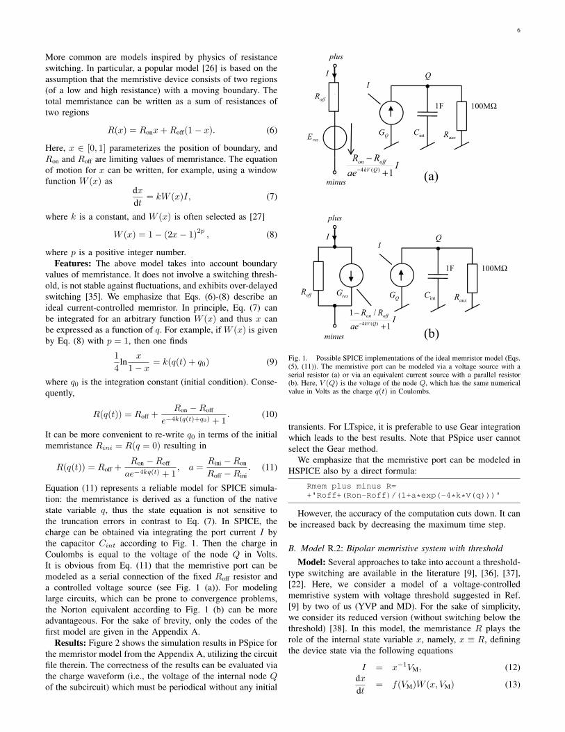
Equation (11) represents a reliable model for SPICE simula-tion: the memristance is derived as a function of the nativestate variable q, thus the state equation is not sensitive tothe truncation errors in contrast to Eq. (7). In SPICE, thecharge can be obtained via integrating the port current I bythe capacitor Cint according to Fig. 1. Then the charge inCoulombs is equal to the voltage of the node Q in Volts.It is obvious from Eq. (11) that the memristive port can bemodeled as a serial connection of the fixed Roff resistor anda controlled voltage source (see Fig. 1 (a)). For modelinglarge circuits, which can be prone to convergence problems,the Norton equivalent according to Fig. 1 (b) can be moreadvantageous. For the sake of brevity, only the codes of thefirst model are given in the Appendix A.

Results: Figure 2 shows the simulation results in PSpice forthe memristor model from the Appendix A, utilizing the circuitfile therein. The correctness of the results can be evaluated viathe charge waveform (i.e., the voltage of the internal node Qof the subcircuit) which must be periodical without any initial

Fig. 1 (a)

R

plus

I QI

offR

RR

intCauxR

resE QG

1F 100MΩ

Iae

RRQkVoffon

1)(4 +−

−

minus

plus

(a)

plus

II

1F 100MΩ

Q

offR

minus

intCauxRresG

QG

I

aeRR

QkVoffon

1/1

)(4 +−

−

(b)

Fig. 1. Possible SPICE implementations of the ideal memristor model (Eqs.(5), (11)). The memristive port can be modeled via a voltage source with aserial resistor (a) or via an equivalent current source with a parallel resistor(b). Here, V (Q) is the voltage of the node Q, which has the same numericalvalue in Volts as the charge q(t) in Coulombs.

transients. For LTspice, it is preferable to use Gear integrationwhich leads to the best results. Note that PSpice user cannotselect the Gear method.

We emphasize that the memristive port can be modeled inHSPICE also by a direct formula:

Rmem plus minus R=+'Roff+(Ron-Roff)/(1+a*exp(-4*k*V(q)))'

However, the accuracy of the computation cuts down. It canbe increased back by decreasing the maximum time step.

B. Model R.2: Bipolar memristive system with threshold

Model: Several approaches to take into account a threshold-type switching are available in the literature [9], [36], [37],[22]. Here, we consider a model of a voltage-controlledmemristive system with voltage threshold suggested in Ref.[9] by two of us (YVP and MD). For the sake of simplicity,we consider its reduced version (without switching below thethreshold) [38]. In this model, the memristance R plays therole of the internal state variable x, namely, x ≡ R, definingthe device state via the following equations

I = x−1VM, (12)dxdt

= f(VM)W (x, VM) (13)

7

10mA

Fig. 2(a)

-10mA

0A

SEL>>

1.0V1

10mA2

V(in)

-1.0V -0.5V 0V 0.5V 1.0VI(Xmem.Eres)

10mA

0V 0A(b)

2.0mV1 V(in) 2 I(Xmem.Eres)

-1.0V -10mA >>

0V

1.0mV

(c)

Time

0s 2s 4s 6s 8s 10sV(Xmem.q)

-1.0mV

Fig. 2. PSpice outputs for the case of an ideal memristor driven by thesine-wave 1V/1Hz voltage source: (a) current-voltage pinched hysteresis loop,(b) voltage and current waveforms, and (c) charge (i.e., integral of current)waveform.

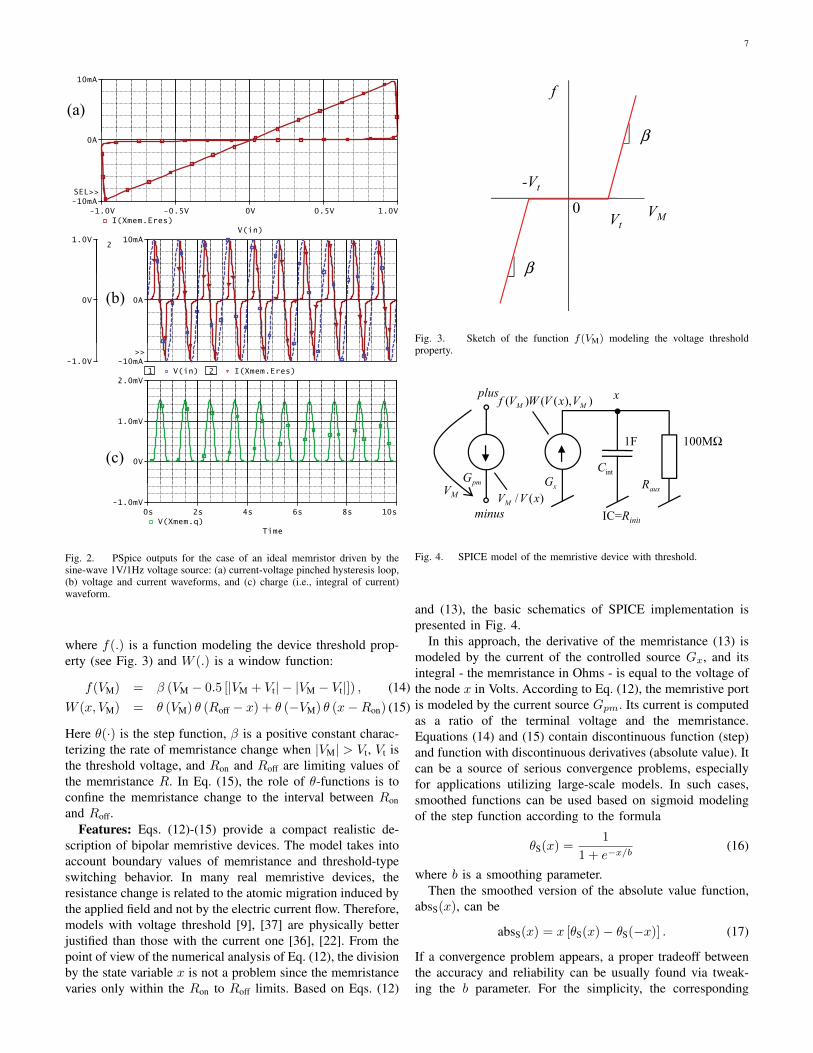
where f(.) is a function modeling the device threshold prop-erty (see Fig. 3) and W (.) is a window function:

f(VM) = β (VM − 0.5 [|VM + Vt| − |VM − Vt|]) , (14)W (x, VM) = θ (VM) θ (Roff − x) + θ (−VM) θ (x−Ron) .(15)

Here θ(·) is the step function, β is a positive constant charac-terizing the rate of memristance change when |VM| > Vt, Vt isthe threshold voltage, and Ron and Roff are limiting values ofthe memristance R. In Eq. (15), the role of θ-functions is toconfine the memristance change to the interval between Ronand Roff.

Features: Eqs. (12)-(15) provide a compact realistic de-scription of bipolar memristive devices. The model takes intoaccount boundary values of memristance and threshold-typeswitching behavior. In many real memristive devices, theresistance change is related to the atomic migration induced bythe applied field and not by the electric current flow. Therefore,models with voltage threshold [9], [37] are physically betterjustified than those with the current one [36], [22]. From thepoint of view of the numerical analysis of Eq. (12), the divisionby the state variable x is not a problem since the memristancevaries only within the Ron to Roff limits. Based on Eqs. (12)

VM

f

0Vt

β

β

-Vt

Fig. 3. Sketch of the function f(VM) modeling the voltage thresholdproperty.

Fig. 4

plus x)),(()( MM VxVWVf

minus

VM

intCauxRpmG xG

1F

IC=R

100MΩ

)(/ xVVMminus IC=Rinit

Fig. 4. SPICE model of the memristive device with threshold.

and (13), the basic schematics of SPICE implementation ispresented in Fig. 4.

In this approach, the derivative of the memristance (13) ismodeled by the current of the controlled source Gx, and itsintegral - the memristance in Ohms - is equal to the voltage ofthe node x in Volts. According to Eq. (12), the memristive portis modeled by the current source Gpm. Its current is computedas a ratio of the terminal voltage and the memristance.Equations (14) and (15) contain discontinuous function (step)and function with discontinuous derivatives (absolute value). Itcan be a source of serious convergence problems, especiallyfor applications utilizing large-scale models. In such cases,smoothed functions can be used based on sigmoid modelingof the step function according to the formula

θS(x) =1

1 + e−x/b(16)

where b is a smoothing parameter.Then the smoothed version of the absolute value function,

absS(x), can be

absS(x) = x [θS(x)− θS(−x)] . (17)

If a convergence problem appears, a proper tradeoff betweenthe accuracy and reliability can be usually found via tweak-ing the b parameter. For the simplicity, the corresponding

8

smoothed functions stpS(x), absS(x) and the functions fS(x)and WS(x) derived from them are defined in the source codesB directly within the individual subcircuits.

Results: Examples of the PSpice outputs, generated fromthe source codes from the Appendix B, are shown in Fig. 5.As follows from Fig. 3, the function f(VM) generates narrowpulses when the memristive device is excited by sine-wavevoltage VM with the amplitude Vmax > Vt. Considering thepositive pulse in Fig. 5, it will be integrated into the voltageof the node x until the memristance R = V (x) approachesits boundary value Roff. At this instant, the window functionW and also the current of the source Gx are set to zero, andthe memristance is fixed to the value Roff. This state persistsuntil the voltage VM drops below the negative threshold level−Vt. Then the function f(VM) becomes negative. It causes thenegative current pulse of the source Gx, and its integral willdecrease the memristance towards Ron. It is obvious from Fig.5 that, although the memristance did not drop to its bottomlimit, the current is cut off at the instant when the voltage VMhas exceeded the threshold Vt (the effect of the window W ).The memristance is held on the low level all the time whenthe voltage VM travels within the stable zone between boththreshold levels. Then the system continues in the motion inthe frame of its periodical steady state.

It follows from the above analysis that the combinationof unreasonably time step and error criteria can result inan incorrect determination of the boundary conditions inthe integration of current pulses. If this happens, then thesimulated waveforms can be distorted due to significant errors.One can make certain of this via step-by-step selection ofvarious parameters/options of the transient analysis or errorcriteria. To identify incorrect results or to achieve the necessaryaccuracy, we can use the following guides (they are true forthe specific netlist in the Appendix B):

1) The upper level of the memristance (the curveV(Xmem.x)) must be Roff. Each declination from thisvalue is a numerical error.

2) The bottom value of the memristance (if it does notreach the boundary Ron, see Fig. 5), must be

Roff −β

2πfVt

2

√(VmaxVt

)2

− 1− π + 2 sin−1 Vt

Vmax

(18)where f is the signal frequency.

For the simulation example from Fig. 5, the necessaryaccuracy can be accomplished e.g. via a low relative errorRELTOL=1u in combination with the maximum time stepequal to one thousandth of the simulation time. Then forPSpice results in Fig. 5, the low-level memristance is 3.1819kΩ whereas the accurate value according to (18) is 3.1847kΩ. Note that the simulation in HSPICE according to code Bprovides even more accurate computation. If the simulationprogram enables to select the integration method, then theGear integration is preferable in this case due to its stabilitythroughout the analysis over many repeating periods.

Note that the current of the source Gx in the SPICE code Bis multiplied by a number 1p and that the integrating capacitorhas the capacitance of 1 pF. It is due to the optimization

Fig. 5

2.0mA

(a)

0A

4.0A V(1)

-6.0V -4.0V -2.0V 0V 2.0V 4.0V 6.0VI(Xmem.Gpm)

-2.0mA

0A

(b)

5.0V1

2.0mA2

12KV3

I(Xmem.Gx)-4.0ASEL>>

I(Xmem.Gx)

0V 0A

4KV

8KV(c)

Time

0s 50ns 100ns1 V(1) 2 I(Xmem.Gpm) 3 V(Xmem.x)

-5.0V -2.0mA 0V >>

Fig. 5. PSpice outputs for the memristive device with threshold driven bya sine-wave excitation. The parameters are defined in the SPICE code in theAppendix B.

of the dynamic range of the source current. Without thismultiplication, the current would reach extreme values of 4TA, which is not optimal with regard to the standard analysisoptions. In addition, since the voltage of the node x in voltsis equal to the memristance in Ohms, this voltage appears inkiloVolts, being also out of the typical values. That is why, ifnecessary, the following optimization step would lead to setand compute the memristance in kiloOhms, not in Ohms, withan increase of the capacitance Cint by three orders to 1nF.Then the voltage V (x) would appear on the common levelof Volts. HSPICE provides the most accurate results amongall three simulation programs. The option RUNLVL=6 forcesHSPICE into the regime of enhanced precision (see SectionVI).

C. Model R.3: Phase change memristive system

Model: In phase change memory (PCM) cells [39], the in-formation storage is based on the reversible phase transforma-tion of relevant materials. In terms of memristive formalism,PCM cells can be described as unipolar second-order current-or voltage- controlled memristive systems. Following generalideas of Ref. [40], we consider here a simple model of PCMcells based on equations describing thermal and phase change

9

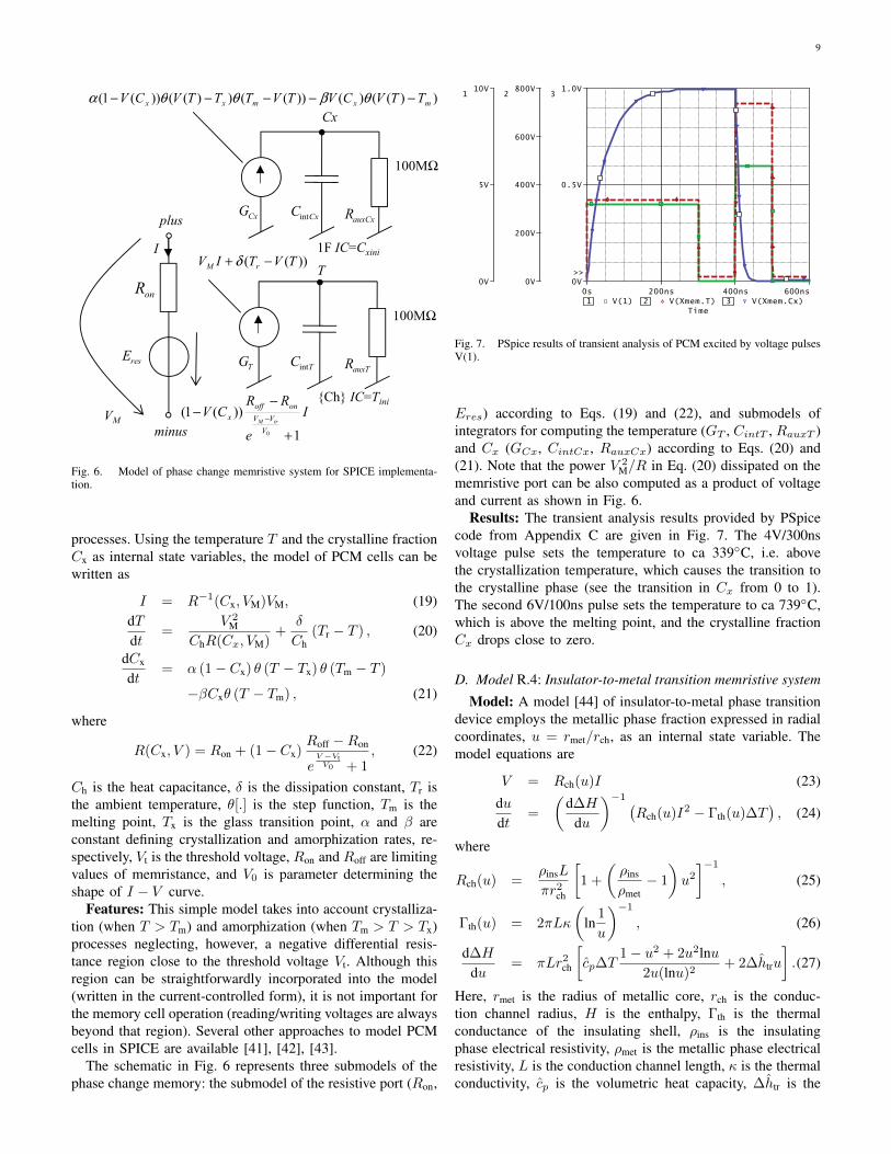
Fig. 6. Model of phase change memristive system for SPICE implementation.

onR

minus

plus

I

CxCint auxCxR

resE

CxG

100MΩ

Cx

1F IC=Cxini

VM I

e

RRCV

V

VV

onoffx

trM

1

))(1(0 +

−− −

TCint auxTRTG

100MΩ

T

))(()())(())(())(1( mxmxx TTVCVTVTTTVCV −−−−− θβθθα

))(( TVTIV rM −+ δ

Ch IC=Tini

Fig. 6. Model of phase change memristive system for SPICE implementa-tion.

processes. Using the temperature T and the crystalline fractionCx as internal state variables, the model of PCM cells can bewritten as

I = R−1(Cx, VM)VM, (19)dTdt

=V 2

M

ChR(Cx, VM)+

δ

Ch(Tr − T ) , (20)

dCx

dt= α (1− Cx) θ (T − Tx) θ (Tm − T )

−βCxθ (T − Tm) , (21)

where

R(Cx, V ) = Ron + (1− Cx)Roff −Ron

eV−VtV0 + 1

, (22)

Ch is the heat capacitance, δ is the dissipation constant, Tr isthe ambient temperature, θ[.] is the step function, Tm is themelting point, Tx is the glass transition point, α and β areconstant defining crystallization and amorphization rates, re-spectively, Vt is the threshold voltage, Ron and Roff are limitingvalues of memristance, and V0 is parameter determining theshape of I − V curve.

Features: This simple model takes into account crystalliza-tion (when T > Tm) and amorphization (when Tm > T > Tx)processes neglecting, however, a negative differential resis-tance region close to the threshold voltage Vt. Although thisregion can be straightforwardly incorporated into the model(written in the current-controlled form), it is not important forthe memory cell operation (reading/writing voltages are alwaysbeyond that region). Several other approaches to model PCMcells in SPICE are available [41], [42], [43].

The schematic in Fig. 6 represents three submodels of thephase change memory: the submodel of the resistive port (Ron,

Fig. 7. PSpice results of transient analysis of PCM excited by voltage pulses V(1).

Time

0s 200ns 400ns 600ns1 V(1) 2 V(Xmem.T) 3 V(Xmem.Cx)

0V

5V

10V1

0V

200V

400V

600V

800V2

0V

0.5V

1.0V3

>>

Fig. 7. PSpice results of transient analysis of PCM excited by voltage pulsesV(1).

Eres) according to Eqs. (19) and (22), and submodels ofintegrators for computing the temperature (GT , CintT , RauxT )and Cx (GCx, CintCx, RauxCx) according to Eqs. (20) and(21). Note that the power V 2

M/R in Eq. (20) dissipated on thememristive port can be also computed as a product of voltageand current as shown in Fig. 6.

Results: The transient analysis results provided by PSpicecode from Appendix C are given in Fig. 7. The 4V/300nsvoltage pulse sets the temperature to ca 339C, i.e. abovethe crystallization temperature, which causes the transition tothe crystalline phase (see the transition in Cx from 0 to 1).The second 6V/100ns pulse sets the temperature to ca 739C,which is above the melting point, and the crystalline fractionCx drops close to zero.

D. Model R.4: Insulator-to-metal transition memristive system

Model: A model [44] of insulator-to-metal phase transitiondevice employs the metallic phase fraction expressed in radialcoordinates, u = rmet/rch, as an internal state variable. Themodel equations are

V = Rch(u)I (23)

dudt

=

(d∆H

du

)−1 (Rch(u)I2 − Γth(u)∆T

), (24)

where

Rch(u) =ρinsL

πr2ch

[1 +

(ρins

ρmet− 1

)u2]−1

, (25)

Γth(u) = 2πLκ

(ln

1

u

)−1

, (26)

d∆H

du= πLr2ch

[cp∆T

1− u2 + 2u2lnu2u(lnu)2

+ 2∆htru

].(27)

Here, rmet is the radius of metallic core, rch is the conduc-tion channel radius, H is the enthalpy, Γth is the thermalconductance of the insulating shell, ρins is the insulatingphase electrical resistivity, ρmet is the metallic phase electricalresistivity, L is the conduction channel length, κ is the thermalconductivity, cp is the volumetric heat capacity, ∆htr is the

10

Fig. 8

plus see Eq. (24)

R

I

CG G

10GΩ

u

1pF

dtdu1210−

fixR

minus

uC auxRvarGuG

VVuVG ))((var IC=uini

see Eq. (30)

Fig. 8. Model of phase change memristive system for SPICE implementa-tion.

Fig. 9

VDC 1 8VRL

4.2k

Re

2.7k

XIMTM

1 2 3

VDC 1.8V

Rscope

50Cp 23pXIMTM

40

Fig. 9. Insulator-to-metal transition memristive system (XIMTM) as a partof the relaxation oscillator [44].

volumetric enthalpy of transformation. Typical values of modelparameters can be found in Ref. [44].

Features: This model describes unipolar current-controlledmemristive device based on a thermally-driven insulator-to-metal phase transition. As demonstrated in [44], it providesrealistic modeling of complex dynamic behavior of the deviceincluding sub-nanosecond switching times. On the other hand,the structure of Eqs. (26) and (27), containing logarithms ofthe phase composition state variable u, divisions by u, anddivisions by logarithm of u, where u can vary between 0 and1, indicates potential numerical problems. To prevent them, itis useful to provide artificial limitations of the variable u inSPICE code.

Equations (23) and (25) can be rewritten in the form

I = R−1fix V +Gvar(u)V, (28)

Rfix =ρinsL

πr2ch, (29)

Gvar(u) =πr2ch

L

(1

ρmet− 1

ρins

)u2. (30)

The corresponding modeling of the memristive port via aparallel combination of a resistor Rfix and a controlled currentsource Gvar is shown in Fig. 8. The variable u is found throughthe integration of the right-side of Eq. (24) using a capacitorCu which is charged by a current source Gu. Since the timederivatives of u come up to high values, a proper scaling bythe factor of 10−12 is provided according to Fig. 8 to preventconvergence problems.

Results: For demonstrating the features of the correspond-

Fig. 10

200uA

300uA1

400mV

600mV2

0A

100uA

0V

200mV

>>

400uA1 600mV2

Time

9.761us 9.762us 9.763us 9.764us 9.765us1 I(XIMTM.Vsense) 2 V(XIMTM.u)

0A 0V

V(XIMTM.u) (a)

200uA

200mV

400mV

Time

8.0us 8.5us 9.0us 9.5us 10.0us1 I(XIMTM.Vsense) 2 V(XIMTM.u)

0ASEL>>

0VSEL>>

(b)

Fig. 10. Transient analysis of circuit from Fig. 9 in PSpice: current pulsesthrough the memristive system (solid lines), phase composition state variableu (dashed lines).

ing SPICE model R.4 in Appendix D, the simulation of theexperimental Pearson-Anson relaxation oscillator, described in[44], has been performed. As shown in Fig. 9, the oxideswitch is used here as current-controlled NDR (NegativeDifferential Resistor) element. The simulation outputs in Fig.10 correspond to the results originally published in [44].

IV. SPICE MODELING OF MEMCAPACITIVE DEVICES

A. Model C.1: Ideal memcapacitor

Model: A voltage-controlled memcapacitor is defined by[1]

q = C (φ(t))VC, (31)

where

φ(t) =

t∫

0

VC(τ)dτ (32)

is the ”flux”. From application point of view, a memcapacitorswitching between two limiting values of memcapacitancewould be of value. This property is achieved, for example,in the following model resembling the memristor model givenby Eq. (10)

C(φ(t)) = Clow +Chigh − Clow

e−4k(φ(t)+φ0) + 1, (33)

where Clow and Chigh are limiting values of memcapacitance(Clow < Chigh), k is a constant and φ0 is a constant definingthe initial value of the capacitance Cini = C(φ = 0). In termsof the initial capacitance, Eq. (33) can be rewritten as follows:

C(φ(t)) = Clow +Chigh − Clow

ae−4kφ(t) + 1, a =

Chigh − Cini

Cini − Clow(34)

Features: The positive aspects of Eq. (34) model include itssimplicity and switching between two limiting values. Among

11

Fig. 11

l

see Eq. (34)Q

VphiVC *))((plus

phiV

QE

minus

intCauxR

capG

vG

100MΩ

V))(( QVddt

1F

Fig. 11. Model of ideal memcapacitor from Section IV-A.

the negative ones we note a lack of switching threshold,sensitivity to fluctuations, over-delayed switching [35], and apossibility of active behavior [1].

The memcapacitor can be modeled as shown in Fig. 11.The flux is computed as an integral of terminal voltage V :the controlled source Gv whose current is equal to the voltageV charges the capacitor Cint, thus the voltage of the nodephi is equal to the flux. This flux is then used to computethe memcapacitance according to Eq. (34). The charge isprovided as a voltage of node Q of the controlled voltagesource EQ. In such a way, the charge is available as asimulation result for inspection, without a necessity of itssubsequent computation from the terminal current. The chargeis then used for evaluating the terminal current via time-domain differentiation (see the source Gcap).

Note that in the simulation programs, which provide thefeature of direct modeling of the charge sources (e.g. OrCADPSpice v. 16, HSPICE, Micro-Cap), the source Gcap can beimplemented via this kind of source without the use of ddtoperation (see the codes in Appendix E). In case of need,the memcapacitive port can be also modeled as a parallelconnection of a fixed capacitor Clow and a variable capacitoraccording to Eq. (34).

Results: The subcircuit of ideal memcapacitor from Ap-pendix E, based on the model from Fig. 11, is used forsimulating hard- switching phenomena which appear whenexciting the memcapacitor with the parameters given in SPICEcode of this subcircuit by 1V/1Hz sinusoidal voltage source.Figure 12 shows the PSpice outputs.

For checking the accuracy of the computation, severalcriteria can be used, for example the rule of the immediatesteady state. HSPICE provides the best results for Gear methodand with the options RUNLVL=0 and LVLTIM=1.

B. Model C.2: Multilayer memcapacitive system

Model: In a multilayer memcapacitive system, several metallayers are embedded into the dielectric medium separating ca-pacitor plates [45]. Here, we consider the simplest realizationof such system involving two internal metal layers, which canbe described as a first-order charge-controlled memcapacitive

Fig. 12

100pV

(a)

-100pV

0V

SEL>>

100p1

20nA2

V(1)

-1.0V -0.5V 0V 0.5V 1.0VV(XMC.Q)

p

(b)

50p

0A

10nA( )

1.0V1

100pV2

1 V(XMC.Q)/v(1) 2 -I(Vin)0

>>-10nA

(c)

0V 0V

( )

Time

0s 50ms 100ms 150ms 200ms1 V(1) 2 V(XMC.Q)

-1.0V >>

-100pV

Fig. 12. Transient analysis of the ideal memcapacitor using Fig. 11model: (a) pinched hysteresis loop, (b) memcapacitance (dashed blue line)and terminal current (solid red line), (c) terminal voltage (solid blue line) andcharge (dashed red line).

system [45]:

VC = C−1(Q, q)q (35)dQdt

= I12 (36)

where

C(Q, q) =C0

1 + δdQq

, (37)

I12 =S e

2πhδ2

[(U − eV1

2

)e−

4πδ√

2mh

√U− eV1

2 −

−(U +

eV12

)e−

4πδk√

2m

h

√U+

eV12

](38)

if eV1 < U , and

I12 =S e3 V 2

1

4πhUδ2

[e−

4πδ√mU3/2

ehV1 −

−(

1 +2eV1U

)e−

4πδ√mU3/2

ehV1

√1+

2eV1U

](39)

if eV1 > U . Here,

V1 = (q +Q)δ/(Sε0εr) (40)

12

plus

minus

1C

2C

VC

dtdQI =12

I

dtdqI =

I

I2

I2 V1GQ

Fig. 13. Model of two-layer memcapacitive system described by Eqs. (35)-(40).

is the voltage drop across internal layers, Q is the internal layercharge, S is the plate area, d is the distance between plates,δ is the distance between internal layers placed symmetricallybetween the plates, ε0 is the vacuum permittivity, εr is therelative dielectric constant of the insulating material, U is thepotential barrier height between two internal metal layers, mand e are electron mass and charge, respectively, h is thePlanck constant, and C0 = ε0εrS/d is the capacitance of thesystem without internal metal layers. Note that Eqs. (38) and(39) are given for V1 > 0. For V1 < 0, the sign of I12 shouldbe changed and |V1| should be used in Eqs. (38), (39).

Features: Multilayer memcapacitive system is an exampleof memory device with the possibility of zero and negativeresponse [35]. As such, hysteresis curves of this device maynot pass through the origin [45], [35]. It is shown in [45]that the multilayer memcapacitive system can be modeledby an equivalent circuit, consisting of linear capacitors andnonlinear resistors. For the case of two layers, such circuitis modified to the form in Fig. 13, with nonlinear resistormodeled via a controlled current source GQ. It can be shownthat if capacitances C1 and C2 are set to values

C1 =ε0εrS

d− δ =C0

1− δ/d , C2 =ε0εrS

δ=

C0

δ/d(41)

and if the current flowing through the source GQ is I12, givenby Eqs. (38) and (39), then the circuit in Fig. 13 behaves asmemcapacitive system with the memcapacitance given by Eq.(37), and that the voltage across C2 is the voltage (40) acrossthe internal layers. Then I2 = I − I12 = d(q − Q)/dt andthus C2 is charged to the charge q −Q. The voltage V1 willbe (q − Q)/C2 which gives Eq. (40). The sum of voltagesacross C1 and C2 is VC = q/C(Q, q) = q/C1 + (q−Q)/C2.After substituting Eqs. (41) we get the formulae (37) for thememcapacitance.

The current I12 from Eqs. (38) and (39), representing formu-lae for current-voltage characteristic of electric tunnel junction,takes the values from a large dynamic range which exceedsthe numerical limits of SPICE-family simulation programs.For typical numerical values given in Appendix F, I12 is ofabout 10−127 for eV1/U = 0.1, 10−116 for eV1/U = 1, 10−56

for eV1/U = 2, and 10−6 for eV1/U = 10. It turns out thatthe low-voltage range eV1 < U (Eq. 38) generates the currentsmuch below the numerical threshold of SPICE, and that thefirst term of Eq. (39) approximates well the I12 versus V1dependence in the form

I12 ≈ aV1|V1|e−b|V1| , a =

Se3

4πhUδ2, b =

4πδ√mU

32

eh(42)

both for positive and negative values of V1. The SPICE codespresented below can be easily modified to include the secondterm of Eq. (39) if required.

To prevent numerical underflow, it is useful to computelogarithm of I12 from (42), to limit artificially its range,and then to compute I12 via inverse logarithm from thislimited values. Examples of the corresponding SPICE codes,providing reliable computation, are given in Appendix F. Notethat due to undocumented errors in OrCAD PSpice v. 16 andHSPICE, they handle incorrectly numerical parameters whichunderflow the limit of ca 10−30. In this model, such parametersare electron mass m and Planck constant h. That is why thecodes for PSpice and HSPICE are modified accordingly forcomputing auxiliary variables a and b from (42) which dependon these quantities.

Results: The SPICE codes from Appendix F can provideall the simulation results from [45]. Figure 14 confirmsthe nonpinched charge-voltage hysteresis loop. This modelenables studying all the interesting phenomena described in[45], including frequency dependent hysteresis, diverging andnegative capacitance.

C. Model C.3: Bistable membrane memcapacitive system

Model: The model of bistable membrane memcapacitivesystem [46] is specified by

q(t) = C(y)V (t), (43)dydτ

= y, (44)

dydτ

= −4π2 y

((y

y0

)2

− 1

)− Γ y −

(β(τ)

1 + y

)2

, (45)

where

C(y) =C0

1 + y, (46)

y0 = z0/d, Γ = 2π γ/ω0, β(t) =[2π/ (ω0 d)]

√C0/ (2m)V (t) and time derivatives are

taken with respect to the dimensionless time τ = t ω0/ (2π).Here, ±z0 are the equilibrium positions of the membrane,d is the separation between the bottom plate and middleposition of the flexible membrane, γ is the damping constant,ω0 is the natural angular frequency of the system, m is themass of the membrane and C0 = ε0 S/d. The dimensionlessmembrane displacement y and membrane’s velocity y playthe role of the internal state variables.

Features: This model describes a memcapacitive devicewith two well-defined equilibrium states ideally suited for

13

Fig. 140V

1.0uV

(a)

1.0u V(2)

-8.0V -4.0V 0V 4.0V 8.0VV(Q)

-1.0uVSEL>>

0

(b)

0A

500uA

0A

500uA2

V(Q) S(I(XMC.GQ))-1.0u

(c)

10V1 -I(Vin) 2 I(XMC.GQ)

-500uA

0A

-500uA

0A

>>

0V(d)

Time

20ms 25ms 30ms 35ms 40ms 45ms 50msV(2)

-10V

Fig. 14. Transient analysis of memcapacitive system from Fig. 13 which isdriven by sinusoidal 7.5V/100Hz voltage source with 1Ohm serial resistance,(a) charge-voltage hysteresis loop, (b) memcapacitor charge (solid blue) andcharge of the internal layers (dashed red), (c) terminal current (solid red) andcurrent I12 (dashed blue), (d) exciting voltage.

binary applications. In order to model reliably the memca-pacitive port, Eqs. (43) and (46) are arranged to the form

V (t) =1

C0q(t) +

y

C0q(t), (47)

which represents the serial connection of two capacitors, withfixed capacitance C0 and with the capacitance dependent onthe variable y (the fact that y can take negative values doesnot cause any problems). The second one is modeled in Fig.15 via a controlled voltage source Ec. The charge, which isnecessary for computing the source voltage, can be obtainedby integrating the terminal current, or more conveniently, it isdirectly the product of voltage across the capacitor C0 andits capacitance. The charge value is available as a voltageof the voltage source EQ. Two classical integrator circuitsprovide the computation of y and y quantities according toEqs. (44) and (45), representing them as voltages of nodesy and yd. Surprisingly, HSPICE provides low precision ofthe simulated waveforms with this model. The precision isconsiderably increased after modeling the variable part ofthe memcapacitive port directly by a capacitor with formula-controlled capacitance (see the Appendix G).

Fig. 15

Q

plus

0C

C0 V(plus,c)QE

100MΩ1F

)(ydV

0C

c

y

)()( QVyVEyC yRyG

see Eq. (45)

minus

V100MΩ1F

yd

0

)()(CQVyV

cE IC=y0

minus

ydC ydRydG IC=yd0

Fig. 15. Model of bistable membrane memcapacitive system described byEqs. (43)-(46).

Results: Figure 16 shows some outputs of PSpice transientanalysis of bistable memcapacitive device under the sinusoidalexcitation. The simulation model confirms all the phenomenawhich are analyzed in Ref. [46], including the fact that thehysteresis is seen at intermediate frequencies compared to thenatural frequency of the system. This model also offers theability to analyze the dynamics of membrane under the voltagepulse excitation. In addition, the chaotic behavior of the devicecan be observed under the conditions specified in [46].

D. Model C.4: Bipolar memcapacitive system with threshold

Model: Here we consider a generic model of memcapacitivedevices with threshold. This model is formulated similarly tothe model of memristive device with threshold III-B proved tobe useful in many cases. We assume that the memcapacitanceC plays the role of the internal state variable x, namely, x ≡C, defining the device state via the following equations

q = xVC, (48)dxdt

= f(VC)W (x, VC) (49)

where f(.) is a function modeling the device threshold prop-erty (see Fig. 3) and W (.) is a window function:

f(VC) = β (VC − 0.5 [|VC + Vt| − |VC − Vt|]) , (50)W (x, VC) = θ (VC) θ (Chigh − x) + θ (−VC) θ (x− Clow) .(51)

Here θ(·) is the step function, β is a positive constant charac-terizing the rate of memcapacitance change when |VC| > Vt,Vt is the threshold voltage, and Clow and Chigh are limitingvalues of the memcapacitance C. In Eq. (51), the role ofθ-functions is to confine the memcapacitance change to theinterval between Clow and Chigh.

Features: The threshold property is not only a widespreadattribute of many physical devices but also an attractive feature

14

Fig. 1640pV

80pV

(a)

0V

-80pV

-40pV

SEL>>

4.0V1

80pV2

V(2)

-3.0V -2.0V -1.0V -0.0V 1.0V 2.0V 3.0VV(XMC.Q)

80pV

(b)

0V

2.0V

0V

40pV

-2.0V -40pV

Time

16s 17s 18s 19s 20s1 V(1) V(XMC.y) 2 V(XMC.Q)

-4.0V -80pV >>

Fig. 16. Transient analysis of bistable elastic memcapacitive system fromFig. 15 in the periodical steady state under conditions defined in SPICEcodes in Appendix G: (a) charge-voltage pinched hysteresis loop, (b) excitingsinusoidal voltage (dashed blue line), membrane position y (green line),memcapacitor charge (red line).

from the application point of view. While the present model isformulated without keeping any specific memcapacitive devicein mind, its structure is closely related to the model of bipolarmemristive devices with threshold and thus can describe amemcapacitive component of such devices, which might be themajor one in properly designed structures. The positive aspectsof the present model include the existence of the switchingthreshold and limiting values of memcapacitance. We note,however, that such a model may, in some cases, result in anactive device behavior.

Fig. 17 shows two possible models based on Eqs. (48)-(51). Both of them compute uniformly the state variable xvia integrating Eq. (49) (see Gx, Cx, Rx). In the model (a),charge is computed as a product of memcapacitor voltage VCand memcapacitance which is resented by the voltage V (x)(see the controlled source EQ). The memcapacitor current, i.e.time derivative of the charge, is provided by the controlledcurrent source GC . The model (b) avoids the differentiation:the charge is computed via integrating the current IC flowingthrough the memcapacitive port, and the terminal voltage iscomputed as a ratio of the charge and capacitance. The division

Fig. 17 (a) Fig. 17 (b)

plus

Q

V(x)*VC

(a)

CG1F

100MΩ

)),(()( CC VxVWVf x

QE

VC

C

IC=Cinit

100MΩ

minus

xC xRxG))(( QVddt

Q(b)

QC QRQG

100MΩ1Fplus

Q

CI

CI(b)

Q QQ

100MΩ1F

x

)()(

VQV

cE

)),(()( CC VxVWVf

minus xC xRxG)(xV

IC=CinitVC

Fig. 17. Two equivalent models of the memcapacitive device with threshold.

by V (x) is not dangerous since the denominator is changingwithin the limits from Clow to Chigh.

Both models provide good results in PSpice and LTspice.However, simulations in HSPICE are accompanied by seriousaccuracy (model (a)) and convergence (model (b)) problems.Their nature probably consists in undocumented problemsin HSPICE Version A-2008.03. They can be overcome viarunning the HSPICE-RF simulator from the software packageinstead of HSPICE. The Appendix H provides PSpice andLTspice codes based on the model in Fig. 17 (b), and HSPICEcode for the same model which can be run on HSPICE-RF.Fig. 18 shows the simulation results from PSpice, demonstrat-ing the periodical switching of the memcapacitance betweenClow and Chigh states.

V. SPICE MODELING OF MEMINDUCTIVE DEVICES

A. Model L.1: Ideal meminductor

Model: A current-controlled meminductor is defined as [1]

φ = L(q(t))I, (52)

where the charge q(t) is the integral of the current. From appli-cation point of view, a meminductor switching between twolimiting values of meminductance is desirable. Similarly toEqs. (10) and (33), we formulate a model of such meminductoras

L(q(t)) = Llow +Lhigh − Llow

e−4k(q(t)+q0) + 1, (53)

15

500pV

Fig. 18(a)

0V

SEL>>

( )

100uA V(2)

-5.0V 0V 5.0VV(Xmem.Q)

-500pVSEL>>

0A(b)

4.0V1

500pV2

120pV3

I(Xmem.Gx)-100uA

0V 0V

40pV

80pV(c)

Time

20us 40us 60us 80us 100us1 V(2) 2 V(Xmem.Q) 3 V(Xmem.x)

-4.0V -500pV 0V >>

Fig. 18. Transient analysis of the model from Fig. 17(b). Memcapacitivedevice with threshold voltage Vt = 3V is driven by sinusoidal 4V/50kHzsignal: (a) charge-voltage pinched hysteresis loop, (b) time derivative of thememcapacitance (i.e. current charging Cx in Fig. 17), (c) exciting voltage(blue dashed line), memcapacitor charge (red line), memcapacitance (greenline).

Fig. 17

IQVL *))((plus

see Eq. (52)phi

IQVL ))((

E 100MΩ

Q

1F

I

phiEI

minus

intCauxR

LE

QGV))(( phiVddt

1F

Fig. 19. Ideal meminductor implementation in SPICE.

where Llow and Lhigh are limiting values of meminductance(Llow < Lhigh). The meminductance can be derived also as afunction of the initial inductance Lini = L(q = 0):

L(q(t)) = Llow +Lhigh − Llow

ae−4kq(t) + 1, a =

Lhigh − Lini

Lini − Llow(54)

Features: Positive aspects of Eq. (54) model include itssimplicity and switching between two limiting values. Amongthe negative ones we note a lack of switching threshold,sensitivity to fluctuations, over-delayed switching [35], and

Fig. 18

0V

50uV

(a)

-50uV

0V

SEL>>

4.0mV1

20m2

I(Iin)

-5.0mA 0A 5.0mAV(XMC.phi)

(b)

0V 10m

(b)

5.0mA1

50uV2

1 V(1) 2 V(XMC.phi)/ I(Iin)-4.0mV 0

>>

0A 0V

(c)

Time

0s 50ms 100ms 150ms 200ms1 I(Iin) 2 V(XMC.phi)

-5.0mA -50uV >>

Fig. 20. Transient analysis of meminductor from Fig. 19: (a) pinchedhysteresis loop, (b) meminductance (dashed blue line) and terminal voltage(solid red line), (c) terminal current (solid blue line) and flux (dashed redline).

the possibility of active behavior [1]. The meminductor can bemodeled in a similar way as the memcapacitor from SectionIV-A, see Fig. 19. The port current I is integrated into thevoltage of node Q, representing the charge. According to Eqs.(52) and (54), the flux is evaluated as the voltage of thecontrolled voltage source Ephi. This voltage is then used forcomputing the terminal voltage via time-domain differentiation(see the source EL). Note that in the simulation programs,which provide the feature of direct modeling of the fluxsources (e.g. OrCAD PSpice v. 16, HSPICE, Micro-Cap),the source EL can be implemented via this kind of sourcewithout the use of ddt operation (see the codes in AppendixI). If necessary, the meminductive port can be also modeledas a serial connection of a fixed inductor Llow and a variableinductor according to Eq. (54).

Results: Results of the transient analysis in PSpice inFig. 20 were obtained from the code in Appendix I. Thememinductor is driven by the ideal current source, generat-ing sinusoidal 5mA/10Hz waveform. The simulation resultsexhibit all basic fingerprints of the meminductor, i.e. odd-symmetric flux-current pinched hysteresis loop and its high-frequency shrinking property, unambiguous meminductance-

1612

LR

CL2 CM

=L1

Fig. 13. Flux-controlled meminductive system based on the inductivecoupling of a coil L1 with a LCR contour [42]. Here, the mutual inductanceM is equal to k

√L1L2, where 0 ≤ k ≤ 1 is the coupling coefficient.

Fig. 14. Steady-state transient analysis of system from Fig. 13: (a)Meminductance vs. current according to Eq. (47), (b) nonpinched flux-currenthysteresis loop, (c) flux (red line) and terminal current (blue line), (d) currentsthrough L1 (solid red line) and L2 (dashed red line) and voltage across L1

(blue line).

B. Model L.2: Effective meminductive system

Model: Let us consider an example of an effective memin-ductive system that can be realized using traditional circuitelements [42]. It consists of an LCR contour inductivelycoupled to an inductor as shown in Fig. 13. In this scheme, twoinductors L1 and L2 interact with each other magnetically. Thecharge on the capacitor C and the current through the inductorL2 play the role of internal state variables, namely, x1 = qCand x2 = IL2

. The system is described by

φ = L (x2, I) I, (44)dx1dt

= −x2, (45)

dx2dt

=1

L2

(x1C−Rx2 −M

dIdt

), (46)

whereL (x2, I) = L1 +M

x2I

. (47)

Features: The circuit sketched in Fig. 13 does not offer non-volatile information storage and has certain similarities withelastic memcapacitive systems [43]. Additional functionalitiesopen if the resistor or capacitor (or both) is replaced by amemristive or memcapacitive system, respectively. We notethat although dI/dt enters into the right-hand-side of Eq. (46)and thus this equation differs from the canonical equations ofmeminductive systems [1], such a definition of meminductivesystem can be considered as a reduced (effective) one [44] thatcan be written in the canonical form using additional internalstate variables [44].

Results: Since the circuit in Fig. 13 is a simple lineardynamical system containing conventional passive elements,its SPICE modeling does not require any special approach.Figure 14 shows some results of PSpice transient analysis.The inductor L1 is driven by a current source with sinusoidal1mA/100kHz waveform. Since x2 = I(L2), the effectivememinductance according to Eq. (47) depends on the ratioof currents flowing through inductors L2 and L1. It is obviousfrom the waveforms I(L1) and I(L2) in Fig. 14 (d) that thememinductance can take infinite values when I(L1) crosseszero level and that both positive and negative values can bepossible. This fact is confirmed in Fig. 14 (a). Figure 14(c) shows that, due to the frequency dependent phase shiftbetween flux and exciting current, the zero-crossing points ofthese waveforms are not identical, and thus the flux-currenthysteresis loop in Fig. 14 (b) cannot be pinched.

VI. CONCLUSIONS

APPENDIX ASPICE CODES FOR MODEL R.1

PSpice and LTspice code.subckt memristorR1 plus minus params: Ron=100 Roff=10k Rini=5k.param uv=10f D=10n k=uv*Ron/D**2 a=(Rini-Ron)/(Roff-Rini)*model of memristive portRoff plus aux RoffEres aux minus value=(Ron-Roff)/(1+a*exp(-4*k*V(q)))*I(Eres)*end of the model of memristive port*integrator modelGQ 0 Q value=i(Eres)Cint Q 0 1Raux Q 0 100meg*end of integrator model*alternative integrator model; SDT function for PSpice must be replaced by IDT for LTspice;Eq Q 0 value=SDT(I(Eres)).ends memristorR1

.options method=gear ;use only for LTspiceVin in 0 sin 0 1 1Xmem in 0 memristorR1.tran 0 20 0 1m; for LTspice, 1m can be replaced by larger step ceiling (up to 200m).probe.end

Fig. 21. Flux-controlled meminductive system based on the inductivecoupling of a coil L1 with a LCR contour [47]. Here, the mutual inductanceM is equal to k

√L1L2, where 0 ≤ k ≤ 1 is the coupling coefficient.

charge state map, etc.

B. Model L.2: Effective meminductive system

Model: Let us consider an example of an effective memin-ductive system that can be realized using traditional circuitelements [47]. It consists of an LCR contour inductivelycoupled to an inductor as shown in Fig. 21. In this scheme, twoinductors L1 and L2 interact with each other magnetically. Thecharge on the capacitor C and the current through the inductorL2 play the role of internal state variables, namely, x1 = qCand x2 = IL2

. The system is described by

φ = L (x2, I) I, (55)dx1dt

= −x2, (56)

dx2dt

=1

L2

(x1C−Rx2 −M

dIdt

), (57)

whereL (x2, I) = L1 +M

x2I

. (58)

Features: The circuit sketched in Fig. 21 does not offer non-volatile information storage and has certain similarities withelastic memcapacitive systems [48]. Additional functionalitiesopen if the resistor or capacitor (or both) is replaced by amemristive or memcapacitive system, respectively. We notethat although dI/dt enters into the right-hand-side of Eq. (57)and thus this equation differs from the canonical equations ofmeminductive systems [1], such a definition of meminductivesystem can be considered as a reduced (effective) one [12] thatcan be written in the canonical form using additional internalstate variables [12].

Results: Since the circuit in Fig. 21 is a simple lineardynamical system containing conventional passive elements,its SPICE modeling does not require any special approach.Figure 22 shows some results of PSpice transient analysis.The inductor L1 is driven by a current source with sinusoidal1mA/100kHz waveform. Since x2 = I(L2), the effectivememinductance according to Eq. (58) depends on the ratioof currents flowing through inductors L2 and L1. It is obviousfrom the waveforms I(L1) and I(L2) in Fig. 22 (d) that thememinductance can take infinite values when I(L1) crosseszero level and that both positive and negative values can bepossible. This fact is confirmed in Fig. 22 (a). Figure 22(c) shows that, due to the frequency dependent phase shift

Fig. 200

2.0m

(a)

I(I)

-10uA -5uA 0A 5uA 10uAV(flux)/I(L1)

-2.0mSEL>>

0V

2.0nV

(b)

2.0nV1 1.0mA2

I(I)

-1.0mA -0.5mA 0A 0.5mA 1.0mAV(flux)

-2.0nV

( )

1 V(fl ) 2 I(I)-2.0nV

0V

-1.0mA

0A

>>

(c)

0A

1.0mA1

0V

1.0mV2

1 V(flux) 2 I(I)

(d)

Time

40us 45us 50us 55us 60us1 I(L1) I(L2) 2 V(in)

-1.0mA -1.0mV >>

Fig. 22. Steady-state transient analysis of system from Fig. 21: (a)Meminductance vs. current according to Eq. (58), (b) nonpinched flux-currenthysteresis loop, (c) flux (red line) and terminal current (blue line), (d) currentsthrough L1 (solid red line) and L2 (dashed red line) and voltage across L1

(blue line).

between flux and exciting current, the zero-crossing points ofthese waveforms are not identical, and thus the flux-currenthysteresis loop in Fig. 22 (b) cannot be pinched.

C. Model L.3: Bipolar meminductive system with threshold

Model: Here we consider a generic model of meminductivedevices with current threshold. This model is formulatedsimilarly to the model of memristive device with thresholdproved to be useful in many cases. We assume that thememinductance L plays the role of the internal state variablex, namely, x ≡ L, defining the device state via the followingequations

φ = LI, (59)dxdt

= f(I)W (x, I) (60)

where f(.) is a function modeling the device threshold prop-erty (see Fig. 3) and W (.) is a window function:

f(I) = β (I − 0.5 [|I + It| − |I − It|]) , (61)W (x, I) = θ (I) θ (Lhigh − x) + θ (−I) θ (x− Llow) .(62)

Here θ(·) is the step function, β is a positive constant charac-terizing the rate of meminductance change when |I| > It, It isthe threshold current, and Llow and Lhigh are limiting values of

17

Fig. 22 (a) Fig. 22 (b)

plus

phi

V(x)*I

(a)

)),(()( IxVWIf

I

LE1F

100MΩ

x

phiE

VL

IC=Linit

100MΩ

minus

intCauxRxG

))(( phiVddt

hi(b)

phiC phiRphiG

100MΩ1Fplus

phiLV

I

(b)

phi pphi

100MΩ1F

x

)()(

xVphiV

LG

V

)),(()( IxVWIf

minus xC xRxG)(xV

IC=LinitVL

Fig. 23. Two equivalent models of the meminductive device with threshold.

the meminductance L. In Eq. (62), the role of θ-functions isto confine the meminductance change to the interval betweenLlow and Lhigh.

Features: The threshold property is not only a widespreadattribute of many physical devices but also an attractive featurefrom the application point of view. The present model, how-ever, is formulated without keeping any specific meminductivedevice in mind. The positive aspects of this model include theexistence of the switching threshold and limiting values ofmeminductance. We note, however, that such a model may, insome cases, result in an active device behavior.

Two kinds of SPICE-oriented models of the meminductivesystem with threshold are shown in Fig. 23(a) and (b). Inboth cases, the state variable x, denoting the meminductance,is represented by the voltage of the node x which is computedvia time-domain integration according to Eq. (60). For model(a), the flux is computed via the Ephi controlled voltagesource as a product of this meminductance and the currentI flowing through the meminductive port. The port voltage isthen evaluated as time derivative of this flux (see the controlledvoltage source EL). For model (b), the flux is computed viaintegration of the port voltage, and the port current is derivedas a ratio of the flux and the meminductance, thus obeying thedifferentiation.

In PSpice and LTSpice, both models work well. How-ever, HSPICE operates only with the model (a) whereasconvergence problems are reported for model (b). They can

2.0nV

Fig. 23(a)

0V

SEL>>

20A I(Isin)

-10uA -5uA -0uA 5uA 10uA-14uA 14uAV(Xmem.phi)

-2.0nV

0A

(b)

20uA1

400uV2

100uV3

I(Xmem.Gx)-20A

0A 0V

60uV

80uV(c)

Time

40us 60us 80us 100us1 I(Isin) 2 V(1) 3

V(Xmem.x)

-20uA -400uV 40uV >>

Fig. 24. Transient analysis of the model from Fig. 23(a). Meminductivedevice with threshold current It = 10µA is driven by sinusoidal 12µA/50kHzsignal: (a) flux-current pinched hysteresis loop, (b) time derivative of thememinductance (i.e. current charging Cx in Fig. 23), (c) exciting current(blue dashed line), meminductor voltage (red line), meminductance (greenline).

be overcome after running HSPICE RF instead of HSPICE.Appendix K summarizes SPICE codes for more reliable modelin Fig. 23(a). A demonstration of PSpice outputs is shownin Fig. 24. It can be observed that the low level of thememinductance is not Llow but it is preserved to the initialvalue Linit (see Fig. 24 and SPICE code in Appendix K).The boundary value is switched to Llow after increasing themagnitude of the exciting current above a proper value.

VI. SETTING THE ANALYSIS PARAMETERS AND SPICEOPTIONS

In this Section we discuss several rules for solving ac-curacy and convergence problems in SPICE via tweakinganalysis parameters and global settings. The common rulesare described in a number of references including a couple ofexcellent books [28], [29]. Some of the rules discussed beloware focused on the specifics of memelement simulation withinthe transient analysis, which is most frequently used for thistype of components.

Incorrect modeling is a common source of the problemsburdening the transient analysis. The rules of building-upcorrect models of memsystems have been described in SectionII-B, thus they will not be dealt with below. The problemsappearing within the analysis can be of the following two

18

types. Convergence problems: SPICE does not find the so-lution (fatal problems indicating by error message). Accuracyproblems: The solution is found but it is modified by errors(problems which can be hidden particularly if we have noidea of the correct result). Since the attempts at increasingthe accuracy attracts the convergence problems, the transientanalysis of systems requiring extremely high accuracy canbe considered as art of compromise. Ideal memelements ormemristive systems with threshold are typical representativesof the above systems (see models R.1, R.2, C.1, C.4, L.1 andL.3 in Sections III-V). The above convergence and accuracyproblems, if they appear, must be handled in the sequenceas they are mentioned. If the circuit does not converge, onecannot deal with the accuracy of the solution.

Note that the SPICE command for the transient analysis canbe in one of two basic forms:

.TRAN Tprint Tstop [skipbp] (*)or

.TRAN Tprint Tstop Tstart Hmax [skipbp] (**)

with an optional flag skipbp or uic. In addition to thecommands (*), (**), the algorithms of the analysis can beaffected by the attributes defined by the .OPTIONS command,especially the error and other iteration criteria. The transientanalysis has two stages, the DC bias point calculation and thetimepoint sweep analysis. The analysis result depends on thebehavior of the numerical algorithms acting in both stages.The first stage can be skipped via the skipbp flag although itis not generally recommended [28].

Convergence aids for DC bias point computationIf SPICE fails to converge to a DC bias point, it aborts the

Newton-Raphson (NR) iteration and prints the error message”No convergence in DC operating point”. Note that mostsimulation examples from Sections III to V with SPICEcodes from the Appendices, work without any convergenceproblems, since their models were built up according torules from Section II-B. The main difficulties are relatedto implementations of C.4. and L.3 in HSPICE. Moreover,the convergence strongly depends on application deterioratingin circuits leading to large sets of equations. The suggestedsequence of the actions is summarized below.

1) Raise ITL1, i.e. the upper iteration limit of the Newton-Raphson (NR) method from its default value 150 to 500or more via the command.OPTION ITL1=500

2) Via the .NODESET command, set the qualified estima-tion of DC values of as many nodal voltages as possible.

3) Call the Source Stepping algorithm via the command.OPTION ITL6=500

4) Increase the GMIN parameter above its default value10−12Ω−1, for example.OPTION GMIN=1E-10GMIN is estimated as reciprocal value of the smallestparasitic resistance which could be placed across anytwo nodes without influencing the model behavior [29].

5) Consider if the relative error of voltages and currentscan be higher than the default value 0.1%. If yes, then

raise RELTOL:.OPTION RELTOL=0.01

6) Determine the magnitude of the smallest voltage ofinterest, e.g. 1uV, and compute the absolute voltage errorVNTOL=RELTOL*1u =1E-8. Then redefine VNTOLfrom its default value 1uV:.OPTION VNTOL=1E-8If you cannot estimate the smallest voltage, then use therule that VNTOL should be by 6 to 9 orders smallerthan the largest voltage in the circuit [28].

7) Determine the magnitude of the smallest current ofinterest, e.g. 1uA, and compute the absolute current errorABSTOL=RELTOL*1u =1E-8. Then redefine ABSTOLfrom its default value 1pA:.OPTION ABSTOL=1E-8If you cannot estimate the smallest current, then use therule that ABSTOL should be by 6 to 9 orders smallerthan the largest current in the circuit [28].

8) If the above hints do not help, remove the skipbp fromthe .TRAN command. If concrete nodal voltages can beestimated, define them via .IC command

Note that steps 4-7 solve the convergence problems atthe expense of the accuracy. In addition to SPICE stan-dard, HSPICE offers additional convergence aids, particu-larly ”Modified Source-Stepping Algorithm” (MSSA), ”GminRamping” (GMR), and ”Pseudo-Transient Analysis” (PTA).MSSA, which can be enabled via the .OPTION CONVER-GENCE=3, can be used instead of step No. 3). GMR canreplace the step No. 4). It can be initiated as .OPTIONGRAMP=X where X is for example 6. PTA is an efficientgeneralization of the step No. 3). It can be activated via thecommand .OPTION CONVERGENCE=1. Details are avail-able in [30].

If PSpice fails to converge within ITL1 limit, the SourceStepping Algorithm (SSA) is switched on automatically, with-out a possibility of controlling this process by the user. IfSSA also fails to converge, the Gmin Stepping (ramping) canbe initiated via the command .OPTION STEPGMIN. Thismethod is then applied first, and if it will not converge, PSpicecomes to SSA algorithm. If LTspice does not converge, it triesthe algorithms of adaptive GMR, adaptive SSA, and PTA insuccessive steps. The user can deactivate individual algorithmsfrom the queue via the corresponding flags [32].

Convergence aids for timepoint sweep analysisThe DC bias solution is a starting point of the transient anal-

ysis which computes the solution at timepoints via numericalintegration of circuit equations. The methods of the numericalintegration used in SPICE are Backward Euler (BE), Trape-zoidal (TRAP), and Gear (GEAR)). LTspice offers TRAP,GEAR2 (i.e. second-order GEAR), a special modification ofTRAP, and BE (it is initiated by undocumented command.OPTIONS MAXORD=1). PSpice uses only TRAP combinedwith BE. HSPICE provides TRAP and GEAR of orders 1 to6, with GEAR1 being the BE method.

The circuit solution at each timepoint is found via the NRiteration. The timepoints are not evenly spaced on the timeaxis but their density is controlled via the TimeStep Control

19

(TSC) algorithm depending on how fast the circuit voltagesand currents are moving. The SPICE standard defines twomethods of timestep control, Iteration Count (IC) and LocalTruncation Error (LTE). In addition, HSPICE offers the thirdmethod called DVDT Dynamic Timestep [30]. PSpice andLTspice use only LTE method.

The convergence problems appear as a consequence ofthe simultaneous action of NR and TSC algorithms. Theyare accompanied by ”Internal Timestep Too Small” or ”NoConvergence During Transient Analysis” error messages, indi-cating that the solution was not found even though the timestepreached its minimum allowable limit. In the first step, it shouldbe checked if the improper model of the circuit is not the keysource of convergence problems (see Section II-B). The otherrecommended steps are summarized below.

1) Raise ITL4, i.e. the upper iteration limit at each time-point, to 50 or more via the command.OPTION ITL4=50

2) Select GEAR2 integration method (not for PSpice).3) Loosen error criteria of NR algorithm according to

steps 5-7 from the Convergence aids for DC bias pointcomputation.

4) Increase TRTOL tentatively above its default value (7for HSPICE, 1 for LTspice).

Accuracy aids for transient analysis of memsystemsAfter resolving prospective convergence problems, the op-

tions of NR and TSC algorithms can be tweaked to maximizethe accuracy. Note that there are two fundamental limits of theaccuracy increase:

• numerical limits in the representation of voltages, cur-rents, and system variable TIME as well as numericalnoise which can be amplified or accumulated by thecircuit model (see Section II-B, Item 3),

• increase of the accuracy promotes the convergence prob-lems.

SPICE provides the following options for increasing the ac-curacy of the transient analysis: Selection of the integrationmethod (not in PSpice), selection of the type of TSC algorithm(not in PSpice and LTspice) and its parameters, selection ofthe parameters of the NR algorithm and .TRAN commandoptions. In addition to the above tools, it is important tofind a suitable guideline for checking the correctness and theaccuracy of the analysis of concrete systems. Demonstrationsof such guidelines, which start from the fundaments of theanalyzed memelements, in particular of ideal memristor (R.1)and memcapacitor (C.1) or bipolar memristive system (R.2)are given in Sections III and IV.

In virtue of the experience in SPICE simulation of assortedtypes of memristive, memcapacitive and meminductive sys-tems, the key factors influencing the accuracy of the transientanalysis are identified and summarized in the following steps.

1) Tighten RELTOL below its default value 0.001. Set theother error criteria according to steps 6 and 7 from theConvergence aids for DC bias point computation.

2) Analyze if the default value of Gmin=10−12 does notaffect the accuracy. If possible, set Gmin=0 [28].

3) LTspice, HSPICE: Select GEAR2 as integration method.4) The parasitic ringing generated by TRAP method [29]

can be solved either by switching to GEAR2 or via stepNo. 7.

5) The parasitic overshoot generated by GEAR2 method[29] can be solved via step No. 7.

6) Accumulated errors (divergence from the correct solu-tion during long transient run) [29] can be solved viastep No. 7.

7) Tighten maximum timestep Tmax (via parameter Hmaxor Tprint, see details below).

8) Tweaking the options of LTE algorithm of dynamictimestep control [28] (via TRTOL or RELTOL, seedetails below).

9) HSPICE: Select the algorithm of dynamic timestepcontrol and its parameters [30] (see details below).

The recommendation 3) is based on the practice thatGEAR2 method is suitable for the analysis of memelements ofvarious natures. Since the models of memory systems containideal integrators, GEAR2 is a good choice owing to its stablebehavior when evaluating integrals of circuit quantities withinmany repeating periods. In addition, GEAR2 provides goodresults for stiff systems where the signals move too fast withrespect to the actual timestep size. Typical cases are voltage-controlled memcapacitive systems or current-controlled me-minductive systems where the port quantities, namely thecapacitor current and inductor voltage, are computed vianumerical differentiation of controlling voltage and current.Examples are given in Sections IV and V under the codesC.1 and L.1. Though the BE method is the best for stiff sys-tems, we should avoid it because it accumulates errors whenanalyzing integration blocks. PSpice does not provide Gearintegration. Fortunately, PSpice combines TRAP with BE, thisway eliminating trapezoidal oscillations and its negative ef-fects. For memelements with hard-switching effects and othersystems which exhibit fast signal transitions, GEAR2 behaveswell with regard to the accumulated errors. Bipolar memristivesystem R.2 from Section III is a typical representative of suchsystems exhibiting the switching phenomena.

It turns out from the above that GEAR2 can be optimalchoice for memelements. The possible imperfections can besuppressed by decreasing the maximum step size (see below).On the other hand, Gear method may not provide the bestresults, and the standard trapezoidal algorithm can solve thetask in some cases (see memristive systems R.3 and R.4, mem-capacitive systems C.2 and C.3, and meminductive system L.2in Sections III to V). If we can select among the methods, thenit is useful to try out the model behavior with all the methodsand to face the results with the expected waveforms.

After selecting the integration algorithm, increasing theaccuracy and eliminating the inherent parasitic behavior of themethod can be accomplished via tightening the timestep. Anindirect method of tightening the timestep is decreasing themaximum timestep Tmax (see Item 7 in the above steps). InPSpice and LTspice, which utilize the LTE method of dynamictimestep control, Tmax is set as Tmax=MIN(Tstop/50, Hmax).The extended syntax (**) of the .TRAN command should beused with Hmax small enough (e.g. Tstop/1000). In HSPICE,

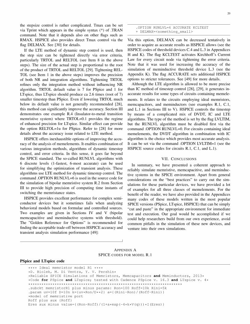
20

the stepsize control is rather complicated. Tmax can be setvia Tprint which appears in the simple syntax (*) of .TRANcommand. Note that it depends also on other flags such asRMAX. HSPICE also provides direct Tmax control via theflag DELMAX. See [30] for details.

If the LTE method of dynamic step control is used, thenthe step size can be tightened directly via error criteria,particularly TRTOL and RELTOL (see Item 8 in the abovesteps). The size of the actual step is proportional to the rootof the product of TRTOL and RELTOL [29]. Tightening REL-TOL (see Item 1 in the above steps) improves the precisionof both NR and integration algorithms. Tightening TRTOLrefines only the integration method without influencing NRalgorithm. TRTOL default value is 7 for PSpice and 1 forLTspice, thus LTspice should produce ca 2.6 times (root of 7)smaller timestep than PSpice. Even if lowering TRTOL muchbelow its default value is not generally recommended [28],this method can significantly improve the accuracy. Section IIIdemonstrates one example R.4 (Insulator-to-metal transitionmemristive system) where TRTOL=0.1 provides the regimeof enhanced precision for LTspice. Similar effect can providethe option RELTOL=1u for PSpice. Refer to [28] for moredetails about the accuracy issue related to LTE method.

HSPICE offers inexhaustible options of improving the accu-racy of the analysis of memelements. It enables combination ofvarious integration methods, algorithms of dynamic timestepcontrol, and error criteria. In this sense, it goes far beyondthe SPICE standard. The so-called RUNLVL algorithms with6 discrete levels (1-fastest, 6-most accurate) can be usedfor simplifying the optimization of transient analysis. Thesealgorithms use LTE method for dynamic timestep control. Thecommand .OPTION RUNLVL=6 is used in the source code forthe simulation of bipolar memristive system R.2 from SectionIII to provide high precision of computing time instants ofswitching the memristance states.

HSPICE provides excellent performance for complex semi-conductor devices but it sometimes fails when analyzingbehavioral models based on formulae and controlled sources.Two examples are given in Sections IV and V (bipolarmemcapacitive and meminductive systems with threshold).The ”Golden Reference for Options” is recommended forfinding the acceptable trade-off between HSPICE accuracy andtransient analysis simulation performance [49]:

.OPTION RUNLVL=6 ACCURATE KCLTEST+ DELMAX=<something_small>

Via this option, DELMAX can be decreased tentatively inorder to acquire as accurate results as HSPICE allows (see theHSPICE codes of threshold devices C.4 and L.3 in AppendicesH and K). The flag KCLTEST activates Kirchhoff’s CurrentLaw for every circuit node via tightening the error criteria.Note that it was used for increasing the accuracy of thesimulation of meminductive threshold device L.3 (see theAppendix K). The flag ACCURATE sets additional HSPICEoptions to stricter tolerances. See [49] for more details.

Although the LTE algorithm is allowed to be more precisethan IC method of timestep control [28], [29], it generates in-accurate results for some types of circuits containing memele-ments. It relates to the circuits employing ideal memristors,memcapacitors, and meminductors (see examples R.1, C.1,and L.1 in Sections III to V). HSPICE controls the timestepby means of a complicated mix of DVDT, IC and LTEalgorithms. The type of the method is set by the flag LVLTIM,but the RUNLVL algorithm must be disabled first via thecommand .OPTION RUNLVL=0. For circuits containing idealmemelements, the DVDT algorithm in combination with ICalgorithm is the choice which provides most accurate analysis.It can be set via the command .OPTION LVLTIM=1 (see theHSPICE source codes for circuits R.1, C.1, and L.1).

VII. CONCLUSIONS

In summary, we have presented a coherent approach toreliably simulate memristive, memcapacitive, and meminduc-tive systems in the SPICE environment. Apart from generalconsiderations on the “best practices” to carry out the sim-ulations for these particular devices, we have provided a lotof examples for all three classes of memelements. For thebenefit of the reader, we have also provided in the Appendicesmany codes of these models written in the most popularSPICE versions (PSpice, LTspice, HSPICE) that can be simply“cut and paste” in the appropriate environment for immediatetest and execution. Our goal would be accomplished if wecould help researchers build from our own experience, avoidcommon pitfalls in the simulation of these new devices, andventure into their own simulations.

APPENDIX ASPICE CODES FOR MODEL R.1

PSpice and LTspice code

**** Ideal memristor model R1 *****D. Biolek, M. Di Ventra, Y. V. Pershin**Reliable SPICE Simulations of Memristors, Memcapacitors and Meminductors, 2013**Code for PSpice and LTspice; tested with Cadence PSpice v. 16.3 and LTspice v. 4***********************************************************************.subckt memristorR1 plus minus params: Ron=100 Roff=10k Rini=5k.param uv=10f D=10n k=uv*Ron/D**2 a=(Rini-Ron)/(Roff-Rini)*model of memristive portRoff plus aux RoffEres aux minus value=(Ron-Roff)/(1+a*exp(-4*k*V(q)))*I(Eres)

21

*end of the model of memristive port*integrator modelGx 0 Q value=i(Eres)Cint Q 0 1Raux Q 0 100meg*end of integrator model*alternative integrator model; SDT function for PSPICE can be replaced by IDT for LTspice*Eq Q 0 value=SDT(I(Eres)).ends memristorR1

*.options method=gear ;use only for LTSpiceVin in 0 sin 0 1 1Xmem in 0 memristorR1.tran 0 10 0 1m.probe.end

HSPICE code

**** Ideal memristor model R1 *****D. Biolek, M. Di Ventra, Y. V. Pershin**Reliable SPICE Simulations of Memristors, Memcapacitors and Meminductors, 2013**Code for HSPICE; tested with HSPICE Version A-2008.03***********************************************************************.subckt memristorR1 plus minus Ron=100 Roff=10k Rini=5k.param uv=10f D=10n k='uv*Ron/D**2' a='(Rini-Ron)/(Roff-Rini)'*model of memristive portRoff plus aux 'Roff'Eres aux minus vol='(Ron-Roff)/(1+a*exp(-4*k*V(q)))*I(Eres)'*end of the model of memristive port*integrator modelGx 0 Q cur='i(Eres)'Cint Q 0 1Raux Q 0 100meg*end of integrator model.ends memristorR1

.options post runlvl=0 lvltim=1 method=gearVin in 0 sin(0,1,1)Xmem in 0 memristorR1.tran 0.1m 10.probe v(x*.*) i(x*.*).end

APPENDIX BSPICE CODES FOR MODEL R.2

PSpice and LTspice code

**** Bipolar memristive system with threshold R2 *****D. Biolek, M. Di Ventra, Y. V. Pershin**Reliable SPICE Simulations of Memristors, Memcapacitors and Meminductors, 2013**Code for PSpice and LTspice; tested with Cadence PSpice v. 16.3 and LTspice v. 4***********************************************************************.subckt memR_TH plus minus PARAMS:+ Ron=1K Roff=10K Rinit=5K beta=1E13 Vt=4.6*model of memristive portGpm plus minus value=V(plus,minus)/V(x)*end of the model of memristive port*integrator modelGx 0 x value=fs(V(plus,minus),b1)*ws(v(x),V(plus,minus),b1,b2)*1pRaux x 0 1TCx x 0 1p IC=Rinit*end of integrator model*smoothed functions.param b1=10u b2=10u.func stps(x,b)=1/(1+exp(-x/b)).func abss(x,b)=x*(stps(x,b)-stps(-x,b)).func fs(v,b)=beta*(v-0.5*(abss(v+Vt,b)-abss(v-Vt,b)))

22

.func ws(x,v,b1,b2)=stps(v,b1)*stps(1-x/Roff,b2)+stps(-v,b1)*stps(x/Ron-1,b2)*end of smoothed functions.ends memR_TH

.options reltol=1u*.options method=gear ;use only for LTspiceVsin 1 0 sin 0 5 50megXmem 1 0 memR_TH.tran 0 0.1u 0 0.1n.probe.end

HSPICE code

**** Bipolar memristive system with threshold R2 *****D. Biolek, M. Di Ventra, Y. V. Pershin**Reliable SPICE Simulations of Memristors, Memcapacitors and Meminductors, 2013**Code for HSPICE; tested with HSPICE Version A-2008.03***********************************************************************.subckt memR_TH plus minus+ Ron=1K Roff=10K Rinit=5K beta=1E13 Vt=4.6*model of memristive portGpm pl mn cur='V(plus,minus)/V(x)'*end of the model of memristive port*integrator modelGx 0 x cur='fs(V(plus,minus),b1)*ws(v(x),V(plus,minus),b1,b2)*1p'Raux x 0 1TCx x 0 1p.IC v(x)='Rinit'*end of integrator model*smoothed functions.param b1=10u b2=10u.param stps(x,b)='1/(1+exp(-x/b))'.param abss(x,b)='x*(stps(x,b)-stps(-x,b))'.param fs(v,b)='beta*(v-0.5*(abss(v+Vt,b)-abss(v-Vt,b)))'.param ws(x,v,b1,b2)='stps(v,b1)*stps(Roff-x,b2)+stps(-v,b1)*stps(x-Ron,b2)'*end of smoothed functions.ends memR_TH

.option post runlvl=6 method=gearVsin 1 0 sin(0,5,50meg)Xmem 1 0 memR_TH.tran 0.1n 0.1u.probe v(x*.*) i(x*.*).end

APPENDIX CSPICE CODE FOR MODEL R.3

PSpice and LTspice code

**** Phase change memristive system R3 *****D. Biolek, M. Di Ventra, Y. V. Pershin**Reliable SPICE Simulations of Memristors, Memcapacitors and Meminductors, 2013**Code for PSpice and LTspice; tested with Cadence PSpice v. 16.3 and LTspice v. 4***********************************************************************.subckt PCM plus minus PARAMS:+ Ron=10K Roff=1meg Rini=100k alpha=20meg beta=100meg+ Tr=20 Tx=200 Tm=600 Tini=20 Ch=2e-15 d=5u+ Vtr=1.8 V0=50m Cxini=0*resistive port modelingRon plus aux RonEres aux minus value=(Roff-Ron)*(1-V(Cx))/(1+exp((V(plus,minus)-Vtr)/V0))*I(Eres)*end of resistive port modeling*temperature computationGT 0 T value=V(plus,minus)*I(Eres)+d*(Tr-V(T))RauxT T 0 100megCintT T 0 Ch IC=Tini*end of temperature computation

23

*Cx computationGCx 0 Cx value=+ alpha*(1-V(Cx))*stps(V(T)/Tx-1)*stps(1-V(T)/Tm)-beta*V(Cx)*stps(V(T)/Tm-1)RauxCx Cx 0 100megCintCx Cx 0 1 IC=Cxini*end of Cx computation*smoothed step function.param b=1m.func stps(x)=1/(1+exp(-x/b))*end of smoothed step function.ends PCM

V 1 0 PWL+ 0 4 300n 4 301n 0 400n 0 401n 6 500n 6 501n 0Xmem 1 0 PCM.tran 0 600n.probe.end

HSPICE code

**** Phase change memristive system R3 *****D. Biolek, M. Di Ventra, Y. V. Pershin**Reliable SPICE Simulations of Memristors, Memcapacitors and Meminductors, 2013**Code for HSPICE; tested with HSPICE Version A-2008.03***********************************************************************.subckt PCM plus minus+ Ron=10K Roff=1meg Rini=100k alpha=20meg beta=100meg+ Tr=20 Tx=200 Tm=600 Tini=20 Ch=2e-15 d=5u+ Vtr=1.8 V0=50m Cxini=0*resistive port modelingRon plus aux 'Ron'Er aux minus vol='(Roff-Ron)*(1-V(Cx))/(1+exp((V(plus,minus)-Vtr)/V0))*I(Er)'*end of resistive port modeling*temperature computationGT 0 T cur='V(plus,minus)*I(Er)+d*(Tr-V(T))'RauxT T 0 100megCintT T 0 'Ch'.IC v(T)='Tini'*end of temperature computation*Cx computationGCx 0 Cx cur=+ 'alpha*(1-V(Cx))*stps(V(T)/Tx-1)*stps(1-V(T)/Tm)-beta*V(Cx)*stps(V(T)/Tm-1)'RauxCx Cx 0 100megCintCx Cx 0 1.IC v(Cx)='Cxini'*end of Cx computation*smoothed step function.param b=1m.param stps(x)='1/(1+exp(-x/b))'*end of smoothed step function.ends PCM

.option postV 1 0 PWL+ 0 4 300n 4 301n 0 400n 0 401n 6 500n 6 501n 0Xmem 1 0 PCM.tran 6n 600n.probe v(x*.*) i(x*.*).end

APPENDIX DSPICE CODE FOR MODEL R.4

PSpice and LTspice code

**** Insulator-to-metal transition memristive system R4 *****D. Biolek, M. Di Ventra, Y. V. Pershin**Reliable SPICE Simulations of Memristors, Memcapacitors and Meminductors, 2013*

24

*Code for PSpice and LTspice; tested with Cadence PSpice v. 16.3 and LTspice v. 4***********************************************************************.subckt IMTM plus minus PARAMS: uini=1u.param deltaT=784 rch=30n L=20n Rhoins=7m Rhomet=100u+ deltaHtr=1.6e8 k=1.5 cp=2.6meg.func Gammath(u)=-2*pi*L*k/log(u).func dHdu(u)=pi*L*rch**2*(cp*deltaT*uExpr(u)+2*deltaHtr*u).func uExpr(u)=(1-u**2+2*u**2*log(u))/(2*u*log(u))**2*resistive port modelingVsense plus sense 0Rfix sense minus Rhoins*L/(pi*rch**2)Gvar sense minus value=V(plus,minus)*v(uL)**2*pi*rch**2/L*(1/Rhomet-1/Rhoins)*end of resistive port modeling*u computationGu 0 u value=1p/dHdu(v(uL))*(v(plus,minus)*I(Vsense)-Gammath(v(uL))*deltaT)Raux u 0 10GCu u 0 1p IC=uini*end of u computation*u limitsEuL uL 0 value=LIMIT(v(u),1u,0.99999)*end of u limits.ends IMTM

*modeling Pearson-Anson relaxation oscillator*.options trtol=0.1 method=gear ; use only in LTSpice.options reltol=1uVdc 1 0 1.8RL 1 2 4.2kRe 2 3 2.7kRscope 4 0 50Cp 2 0 23pXIMTM 3 4 IMTM.tran 0 10u 8u 1n.probe.end

HSPICE code

**** Insulator-to-metal transition memristive system R4 *****D. Biolek, M. Di Ventra, Y. V. Pershin**Reliable SPICE Simulations of Memristors, Memcapacitors and Meminductors, 2013**Code for HSPICE; tested with HSPICE Version A-2008.03***********************************************************************.subckt IMTM plus minus uini=1u.param deltaT=784 rch=30n L=20n Rhoins=7m Rhomet=100u+ deltaHtr=1.6e8 k=1.5 cp=2.6meg.param pi=3.1415926536.param Gammath(u)='-2*pi*L*k/log(u)'.param dHdu(u)='pi*L*rch**2*(cp*deltaT*uExpr(u)+2*deltaHtr*u)'.param uExpr(u)='(1-u**2+2*u**2*log(u))/(2*u*log(u))**2'*resistive port modelingVsense plus sense 0Rfix sense minus 'Rhoins*L/(pi*rch**2)'Gvar sense minus cur='V(plus,minus)*v(uL)**2*pi*rch**2/L*(1/Rhomet-1/Rhoins)'*end of resistive port modeling*u computationGu 0 u cur='1p/dHdu(v(uL))*(v(plus,minus)*I(Vsense)-Gammath(v(uL))*deltaT)'Raux u 0 10GCu u 0 1p.IC v(u)='uini'*end of u computation*u limitsEuL uL 0 vol='min(max(v(u),1u),0.99999)'*end of u limits.ends IMTM

*modeling Pearson-Anson relaxation oscillator.option post runlvl=6Vdc 1 0 1.8RL 1 2 4.2k

25

Re 2 3 2.7kRscope 4 0 50Cp 2 0 23pXIMTM 3 4 IMTM.tran 1n 10u 8u 1n.probe v(x*.*) i(x*.*).end

APPENDIX ESPICE CODE FOR MODEL C.1

PSpice and LTspice code

**** Ideal memcapacitor C1 *****D. Biolek, M. Di Ventra, Y. V. Pershin**Reliable SPICE Simulations of Memristors, Memcapacitors and Meminductors, 2013**Code for PSpice and LTspice; tested with Cadence PSpice v. 16.3 and LTspice v. 4***********************************************************************.subckt memcapacitor plus minus params: Clow=1p Chigh=100p Cini=2p k=100.param a=(Chigh-Cini)/(Cini-Clow)*model of memcapacitive port.func C(phi)=Clow+(Chigh-Clow)/(a*exp(-4*k*phi)+1)EQ Q 0 value=C(V(phi))*V(plus,minus)Gcap plus minus value=ddt(V(Q))*for OrCAD PSpice 16, the above line can be replaced by Gcap plus minus Q=V(Q)*end of the model of memcapacitive port*integrator modelGv 0 phi value=v(plus,minus)Cint phi 0 1Raux phi 0 100meg*end of integrator model.ends memcapacitor

Vin 1 0 sin 0 1 10XMC 1 0 memcapacitor.tran 0 0.2 0 1m.probe.end

HSPICE code

**** Ideal memcapacitor C1 *****D. Biolek, M. Di Ventra, Y. V. Pershin**Reliable SPICE Simulations of Memristors, Memcapacitors and Meminductors, 2013**Code for HSPICE; tested with HSPICE Version A-2008.03***********************************************************************.subckt memcapacitor plus minus Clow=1p Chigh=100p Cini=2p k=100.param a='(Chigh-Cini)/(Cini-Clow)'*model of memcapacitive port.param C(phi)='Clow+(Chigh-Clow)/(a*exp(-4*k*phi)+1)'EQ Q 0 vol='C(V(phi))*V(plus,minus)'CQ plus minus C='C(V(phi))' CTYPE=1*end of the model of memcapacitive port*integrator modelGv 0 phi cur='v(plus,minus)'Cint phi 0 1Raux phi 0 100meg*end of integrator model.ends memcapacitor

.option runlvl=0 lvltim=1 method=gearVin 1 0 sin(0,1,10)XMC 1 0 memcapacitor.tran 1m 0.2.probe v(x*.*) i(x*.*).end

26

APPENDIX FSPICE CODE FOR MODEL C.2

PSpice and LTspice code

**** Multilayer memcapacitive system C2 *****D. Biolek, M. Di Ventra, Y. V. Pershin**Reliable SPICE Simulations of Memristors, Memcapacitors and Meminductors, 2013**Code for PSpice and LTspice; tested with Cadence PSpice v. 16.3 and LTspice v. 4***********************************************************************.subckt MLMCS plus minus params: d=100n del=66.6n Su=100u er=5 Uev=0.33.param e0=8.854p m=9.109e-31 e=1.602e-19 h=6.626e-34.param C0=e0*er*Su/d C1=C0/(1-del/d) C2=C0*d/del*Use this below line for LTSpice*.param a=Su*e**2/(4*pi*h*Uev*del**2) b=4*pi*del*sqrt(m*e)*pwr(Uev,1.5)/h loga=log(a)*Use this below line for OrCAD PSpice.param a=2.10572e5 b=91.4682096 loga=log(a).func I12(V1)=V1*abs(V1)*exp(LIMIT(loga-b/MAX(abs(V1),1n),-20,20))*model of memcapacitive portC1 plus c C1C2 c minus C2GQ c minus value=I12(V(c,minus))Rshunt c 0 100meg*end of the model of memcapacitive port.ends MLMCS

Vin 1 0 sin 0 7.5 100Rin 1 2 1XMC 2 0 MLMCSEQ Q 0 value=-sdt(I(Vin)).tran 0 50m 20m 50u skipbp.probe.end

HSPICE code

**** Multilayer memcapacitive system C2 *****D. Biolek, M. Di Ventra, Y. V. Pershin**Reliable SPICE Simulations of Memristors, Memcapacitors and Meminductors, 2013**Code for HSPICE; tested with HSPICE Version A-2008.03***********************************************************************.subckt MLMCS plus minus d=100n del=66.6n Su=100u er=5 Uev=0.33.param pi=3.1415926536 e0=8.854p m=9.109e-31 e=1.602e-19 h=6.626e-34.param C0='e0*er*Su/d' C1='C0/(1-del/d)' C2='C0*d/del'.param a=2.10572e5 b=91.4682096 loga='log(a)'.param I12(V1)='V1*abs(V1)*exp(min(max(loga-b/MAX(abs(V1),1n),-20),20))'*model of memcapacitive portC1 plus c 'C1'C2 c minus 'C2'GQ c minus cur='I12(V(c,minus))'Rshunt c 0 100meg*end of the model of memcapacitive port.ends MLMCS

.option postVin 1 0 sin(0,7.5,100)Rin 1 2 1XMC 2 0 MLMCS*charge computationGqq qq 0 vol='I(Vin)'Cqq qq 0 1Rqq qq 0 100meg*end of charge computation.tran 50u 50m 20m 50u.probe v(x*.*) i(x*.*).end

27

APPENDIX GSPICE CODE FOR MODEL C.3

PSpice and LTspice code

**** Bistable membrane memcapacitive system C3 *****D. Biolek, M. Di Ventra, Y. V. Pershin**Reliable SPICE Simulations of Memristors, Memcapacitors and Meminductors, 2013**Code for PSpice and LTspice; tested with Cadence PSpice v. 16.3 and LTspice v. 4***********************************************************************.subckt BEMS plus minus params: y0=0.2 yd0=0.param gamma=0.7 b=1 C0=10p*model of memcapacitive portC0 plus c C0Ec c minus value=V(Q)*V(y)/C0*end of the model of memcapacitive port*Q computationEQ Q 0 value=C0*V(plus,c)*end of Q computation*y computationGy 0 y value=v(yd)Cy y 0 1 IC=y0Ry y 0 100meg*end of y computation*yd computationGyd 0 yd value=-(4*pi**2*v(y)*((V(y)/y0)**2-1)+gamma*v(yd)+(b*V(plus,minus)/(1+v(y)))**2)Cyd yd 0 1 IC=yd0Ryd yd 0 100meg*end of yd computation.ends BEMS

Vin 1 0 sin 0 2.8 0.658Rin 1 2 1XMC 2 0 BEMS.tran 0 20 16 4m.probe.end

HSPICE code

**** Bistable membrane memcapacitive system C3 *****D. Biolek, M. Di Ventra, Y. V. Pershin**Reliable SPICE Simulations of Memristors, Memcapacitors and Meminductors, 2013**Code for HSPICE; tested with HSPICE Version A-2008.03***********************************************************************.subckt BEMS plus minus y0=0.2 yd0=0.param pi=3.1415926536 gamma=0.7 b=1 C0=10p*model of memcapacitive portC0 plus c 'C0'CQ c minus C='C0/V(y)' CTYPE=1*Ec c minus vol='V(Q)*V(y)/C0'*end of the model of memcapacitive port*Q computation*GQ 0 Q cur='I(EC)'*CQ Q 0 1*RQ Q 0 100megEQ Q 0 vol='C0*V(plus,c)'*end of Q computation*y computationGy 0 y cur='v(yd)'Cy y 0 1.IC v(y)='y0'Ry y 0 100meg*end of y computation*yd computationGyd 0 yd cur='-(4*pi**2*v(y)*((V(y)/y0)**2-1)+gamma*v(yd)+(b*V(plus,minus)/(1+v(y)))**2)'Cyd yd 0 1.IC v(yd)='yd0'Ryd yd 0 100meg*end of yd computation

28

.ends BEMS

.option post runlvl=6Vin 1 0 sin(0,2.8,0.658)Rin 1 2 1XMC 2 0 BEMS.tran 4m 20 16 4m.probe v(x*.*) i(x*.*).end

APPENDIX HSPICE CODE FOR MODEL C.4

PSpice and LTspice code

**** Bipolar memcapacitive system with threshold C4 *****D. Biolek, M. Di Ventra, Y. V. Pershin**Reliable SPICE Simulations of Memristors, Memcapacitors and Meminductors, 2013**Code for PSpice and LTspice; tested with Cadence PSpice v. 16.3 and LTspice v. 4***********************************************************************.subckt memC_TH plus minus PARAMS:+ Clow=1p Chigh=100p Cinit=50p beta=70u Vt=3*model of memcapacitive portEc plus minus value=V(Q)/V(x)*end of the model of memcapacitive port*integrator modelGx 0 x value=fs(V(plus,minus),b1)*ws(v(x),v(plus,minus),b1,b2)Raux x 0 100megCx x 0 1 IC=Cinit*end of integrator model*charge computationGQ 0 Q value=I(Ec)CQ Q 0 1RQ Q 0 100meg*end of charge computation*smoothed functions.param b1=10m b2=1u.func stps(x,b)=1/(1+exp(-x/b)).func abss(x,b)=x*(stps(x,b)-stps(-x,b)).func fs(v,b)=beta*(v-0.5*(abss(v+vt,b)-abss(v-Vt,b))).func ws(x,v,b1,b2)=stps(v,b1)*stps(1-x/Chigh,b2)+stps(-v,b1)*stps(x/Clow-1,b2)*end of smoothed functions.ends memC_TH

.options reltol=1u ; use 0.1u for LTspice*.options method=gear ;use only for LTspiceVsin 1 0 sin 0 4 50kRi 1 2 1mXmem 2 0 memC_TH.tran 0 100u 20u 0.1u.probe.end

HSPICE code

**** Bipolar memcapacitive system with threshold C4 *****D. Biolek, M. Di Ventra, Y. V. Pershin**Reliable SPICE Simulations of Memristors, Memcapacitors and Meminductors, 2013**Code for HSPICE; tested with HSPICE RF Version A-2008.03***********************************************************************.subckt memC_TH plus minus+ Clow=1p Chigh=100p Cinit=50p beta=70u Vt=3*model of memcapacitive portEc plus minus vol='V(Q)/(V(x))'*end of the model of memcapacitive port*integrator modelGx 0 x cur='fs(V(plus,minus),b1)*ws(v(x),v(plus,minus),b1,b2)'Rx x 0 100megCx x 0 1

29

.IC v(x)='Cinit'*end of integrator model*charge computationGQ 0 Q cur='I(Ec)'CQ Q 0 1RQ Q 0 100meg*end of charge computation*smoothed functions.param b1=10m b2=10u.param stps(x,b)='1/(1+exp(-x/b))'.param abss(x,b)='x*(stps(x,b)-stps(-x,b))'.param fs(v,b)='beta*(v-0.5*(abss(v+Vt,b)-abss(v-Vt,b)))'.param ws(x,v,b1,b2)='stps(v,b1)*stps(1-x/Chigh,b2)+stps(-v,b1)*stps(x/Clow-1,b2)'*end of smoothed functions.ends memC_TH

.option post runlvl=6 delmax=1nVsin 1 0 sin(0,4,50k)Ri 1 2 1Xmem 2 0 memC_TH.tran 0.1u 100u.probe v(x*.*) i(x*.*).end

APPENDIX ISPICE CODE FOR MODEL L.1

PSpice and LTspice code

**** Ideal meminductor L1 *****D. Biolek, M. Di Ventra, Y. V. Pershin**Reliable SPICE Simulations of Memristors, Memcapacitors and Meminductors, 2013**Code for PSpice and LTspice; tested with Cadence PSpice v. 16.3 and LTspice v. 4***********************************************************************.subckt meminductor plus minus params: Llow=1m Lhigh=10m Lini=2m k=10k.param a=(Lhigh-Lini)/(Lini-Llow)*model of meminductive port.func L(q)=Llow+(Lhigh-Llow)/(a*exp(-4*k*q)+1)Ephi phi 0 value=L(V(Q))*I(EL)EL plus minus value=ddt(V(phi))*end of the model of meminductive port*integrator modelGQ 0 Q value=I(EL)Cint Q 0 1Raux Q 0 100meg*end of integrator model.ends meminductor

Iin 0 1 sin 0 5m 10XMC 1 0 meminductor.tran 0 200m 0 200u skipbp ;for LTspice, decrease step ceiling from 200u to 10u.probe.end

HSPICE code

**** Ideal meminductor L1 *****D. Biolek, M. Di Ventra, Y. V. Pershin**Reliable SPICE Simulations of Memristors, Memcapacitors and Meminductors, 2013**Code for HSPICE; tested with HSPICE Version A-2008.03***********************************************************************.subckt meminductor plus minus Llow=1m Lhigh=10m Lini=2m k=10k.param a='(Lhigh-Lini)/(Lini-Llow)'*model of meminductive port.param L(q)='Llow+(Lhigh-Llow)/(a*exp(-4*k*q)+1)'Ephi phi 0 vol='L(V(Q))*I(LL)'LL plus minus L='L(V(Q))' LTYPE=1*end of the model of meminductive port*integrator model

30

GQ 0 Q cur='I(LL)'Cint Q 0 1Raux Q 0 100meg*end of integrator model.ends meminductor

.option post runlvl=0 lvltim=1 method=gearIin 0 1 sin(0,5m,10)XMC 1 0 meminductor.tran 200u 200m.probe v(x*.*) i(x*.*).end

APPENDIX JSPICE CODE FOR MODEL L.2

PSpice and LTspice code

**** Effective meminductive system L2 *****D. Biolek, M. Di Ventra, Y. V. Pershin**Reliable SPICE Simulations of Memristors, Memcapacitors and Meminductors, 2013**Code for PSpice and LTspice; tested with Cadence PSpice v. 16.3 and LTspice v. 4***********************************************************************.subckt MLsystem plus minus params: L1=1u L2=1u k=0.8 R=1 C=1uL1 plus minus L1L2 1 3 L2k L1 L2 kR 1 2 RC 2 3 CRaux 3 0 100meg.ends MLsystem

I 0 in sin 0 1m 100kXML in 0 MLsystemEflux flux 0 value=sdt(v(in)).tran 0 60u 40u 0.5n.probe.end

HSPICE code

**** Effective meminductive system L2 *****D. Biolek, M. Di Ventra, Y. V. Pershin**Reliable SPICE Simulations of Memristors, Memcapacitors and Meminductors, 2013**Code for HSPICE; tested with HSPICE Version A-2008.03***********************************************************************.subckt MLsystem plus minus L1=1u L2=1u k=0.8 R=1 C=1uL1 plus minus L 1L2 1 3 L 2k L1 L2 kR 1 2 RC 2 3 CRaux 3 0 100meg.ends MLsystem

.option postI 0 in sin(0,1m,100k)XML in 0 MLsystemGflux 0 flux cur='v(in)'Cint flux 0 1Rx flux 0 100meg.tran 0.4n 60u 40u 0.5n.probe v(x*.*) i(x*.*).end

APPENDIX KSPICE CODE FOR MODEL L.3

PSpice and LTspice code

31

**** Bipolar meminductive system with threshold L3 *****D. Biolek, M. Di Ventra, Y. V. Pershin**Reliable SPICE Simulations of Memristors, Memcapacitors and Meminductors, 2013**Code for PSpice and LTspice; tested with Cadence PSpice v. 16.3 and LTspice v. 4***********************************************************************.subckt memL_TH plus minus PARAMS:+ Llow=1u Lhigh=100u Linit=50u beta=10meg It=10u*model of meminductive portEL plus minus value=ddt(V(phi))*forOrCADPSpice 16, the above line can be replaced by EL plus minus F=V(phi)*end of the model of meminductive port*integrator modelGx 0 x value=fs(I(EL),b1)*ws(v(x),I(EL),b1,b2)Raux x 0 100megCx x 0 1 IC=Linit*end of integrator model*flux computationEphi phi 0 value=I(EL)*V(x)*end of flux computation*smoothed functions.param b1=10n b2=1u.func stps(x,b)=1/(1+exp(-x/b)).func abss(x,b)=x*(stps(x,b)-stps(-x,b)).func fs(I,b)=beta*(I-0.5*(abss(I+It,b)-abss(I-It,b))).func ws(x,I,b1,b2)=stps(I,b1)*stps(1-x/Lhigh,b2)+stps(-I,b1)*stps(x/Llow-1,b2)*end of smoothed functions.ends memL_TH

.options reltol=1u*.options method=gear ;use only for LTspiceIsin 0 1 sin 0 12u 50kXmem 1 0 memL_TH.tran 0 100u 40u 0.1u.probe.end

HSPICE code

**** Bipolar meminductive system with threshold L3 *****D. Biolek, M. Di Ventra, Y. V. Pershin**Reliable SPICE Simulations of Memristors, Memcapacitors and Meminductors, 2013**Code for HSPICE; tested with HSPICE Version A-2008.03***********************************************************************.subckt memL_TH plus minus+ Llow=1u Lhigh=100u Linit=50u beta=10meg It=10u*model of meminductive portLL plus minus L='V(x)' LTYPE=1*end of the model of meminductive port*integrator modelGx 0 x cur='fs(I(LL),b1)*ws(v(x),I(LL),b1,b2)'Raux x 0 100megCx x 0 1.IC v(x)='Linit'*end of integrator model*flux computationEphi phi 0 vol='I(LL)*V(x)'*end of flux computation*smoothed functions.param b1=10n b2=1u.param stps(x,b)='1/(1+exp(-x/b))'.param abss(x,b)='x*(stps(x,b)-stps(-x,b))'.param fs(I,b)='beta*(I-0.5*(abss(I+It,b)-abss(I-It,b)))'.param ws(x,I,b1,b2)='stps(I,b1)*stps(1-x/Lhigh,b2)+stps(-I,b1)*stps(x/Llow-1,b2)'*end of smoothed functions.ends memL_TH

.option post runlvl=6 KCLTEST delmax=1nIsin 0 1 sin(0,12u,50k)Xmem 1 0 memL_TH

32

.tran 0.1u 100u

.probe v(x*.*) i(x*.*)

.end

ACKNOWLEDGMENT

This work has been partially supported by NSF grantsDMR-0802830 and ECCS-1202383, the Center for MagneticRecording Research at UCSD, the SIX Research Center ofSensor, Information and Communication Systems at BUT, andby the development project K217 at UD.

REFERENCES

[1] M. Di Ventra, Y. V. Pershin, and L. O. Chua, “Circuit elements withmemory: Memristors, memcapacitors, and meminductors,” Proc. IEEE,vol. 97, no. 10, pp. 1717–1724, 2009.

[2] M. Di Ventra and Y. V. Pershin, “The parallel approach,” Nature Physics,vol. 9, pp. 200–202, 2013.

[3] F. Alibart, S. Pleutin, D. Guerin, C. Novembre, S. Lenfant, K. Lmimouni,C. Gamrat, and D. Vuillaume, “An organic nanoparticle transistorbehaving as a biological spiking synapse,” Adv. Funct. Mat., vol. 20,pp. 330–337, 2010.

[4] Y. V. Pershin and M. Di Ventra, “Solving mazes with memristors: amassively-parallel approach,” Phys. Rev. E, vol. 84, p. 046703, 2011.

[5] Y. V. Pershin and M. Di Ventra, “Neuromorphic, digital and quantumcomputation with memory circuit elements,” Proc. IEEE, vol. 100, pp.2071–2080, 2012.

[6] E. Linn, R. Rosezin, S. Tappertzhofen, U. Bottger, and R. Waser, “Be-yond von Neumann-logic operations in passive crossbar arrays alongsidememory operations,” Nanotechnology, vol. 23, no. 30, p. 305205, 2012.

[7] A. Thomas, “Memristor-based neural networks,” Journal of Physics D:Applied Physics, vol. 46, no. 9, p. 093001, 2013.

[8] D. Sacchetto, G. De Micheli, and Y. Leblebici, “Multiterminal Memris-tive Nanowire Devices for Logic and Memory Applications: A Review,”Proc. IEEE, vol. 100, pp. 2008–2020, 2012.

[9] Y. V. Pershin, S. La Fontaine, and M. Di Ventra, “Memristive model ofamoeba learning,” Phys. Rev. E, vol. 80, p. 021926, 2009.

[10] V. Erokhin, T. Berzina, A. Smerieri, P. Camorani, S. Erokhina, andM. Fontana, “Bio-inspired adaptive networks based on organic mem-ristors,” Nano Communication Networks, vol. 1, no. 2, pp. 108–117,2010.

[11] G. K. Johnsen, C. A. Lutken, O. G. Martinsen, and S. Grimnes,“Memristive model of electro-osmosis in skin,” Phys. Rev. E, vol. 83,p. 031916, 2011.

[12] F. L. Traversa, Y. V. Pershin, and M. Di Ventra, “Memory models ofadaptive behaviour,” IEEE Trans. Neural Netw. Learn. Syst. (in press),arXiv:1301.0209, 2013.

[13] L. O. Chua, “Memristor - the missing circuit element,” IEEE Trans.Circuit Theory, vol. 18, pp. 507–519, 1971.

[14] Z. Biolek, D. Biolek, and V. Biolkova, “SPICE model of memristorwith nonlinear dopant drift,” Radioengineering, vol. 18, no. 2, Part 2,pp. 210–214, 2009.

[15] ——, “SPICE modeling of memristive, memcapacitative and memin-ductive systems,” Proc. of ECCTD ’09, European Conference on CircuitTheory and Design, pp. 249–252, August 23-27, 2009.

[16] S. Benderli and T. A. Wey, “On SPICE macromodelling of TiO2memristors,” Electron. Lett., vol. 45, no. 7, pp. 377–378, 2009.

[17] A. Rak and G. Cserey, “Macromodeling of the memristor in SPICE,”IEEE Trans. Comput.-Aided Design Integr. Circuits Syst., vol. 29, pp.632–636, 2010.

[18] D. Biolek, Z. Biolek, and V. Biolkova, “SPICE modelling of memca-pacitor,” El. Lett., vol. 46, pp. 520–522, 2010.

[19] ——, “PSPICE modeling of meminductor,” Analog. Integr. Circ. Sig.Process., vol. 66, pp. 129–137, 2011.

[20] Z. Kolka, D. Biolek, and V. Biolkova, “Hybrid modelling and emulationof mem-systems,” Int. J. Numer. Mod., vol. 25, pp. 216–225, 2011.

[21] Y. V. Pershin and M. Di Ventra, “Spice model of memristive deviceswith threshold,” Radioengineering, vol. 22, no. 2, pp. 485–489, 2013.

[22] S. Kvatinsky, E. G. Friedman, A. Kolodny, and U. C. Weiser, “TEAM:ThrEshold adaptive memristor model,” IEEE Trans. Circ. Syst. I, vol. 60,pp. 211–221, 2013.

[23] Y. V. Pershin and M. Di Ventra, “Teaching Memory Circuit Elementsvia Experiment-Based Learning,” IEEE Circ. Syst. Mag., vol. 12, pp.64–74, 2012.

[24] Z. Kolka, D. Biolek, and V. Biolkova, “Frequency-domain steady-stateanalysis of circuits with mem-elements,” Analog Integrated Circuits andSignal Processing, vol. 74, no. 1, pp. 79–89, 2013.

[25] R. Tetzlaff and et al., “The memristor theory,” in Springer Book (to bepublished). Springer, 2013.

[26] D. B. Strukov, G. S. Snider, D. R. Stewart, and R. S. Williams, “Themissing memristor found,” Nature, vol. 453, pp. 80–83, 2008.

[27] Y. N. Joglekar and S. J. Wolf, “The elusive memristor: properties ofbasic electrical circuits,” Eur. J. Phys., vol. 30, p. 661, 2009.

[28] K. S. Kundert and P. Foreword By-Gray, The Designer’s Guide to SPICEand SPECTRE. Kluwer Academic Publishers, 1995.

[29] R. M. Kielkowski, Inside Spice. McGraw-Hill New York, 1998.[30] HSPICE User Guide: Simulation and Analysis. Synopsys, Version A-

2008.03, 2008.[31] PSpice A/D Reference Guide. Product Version 16.5, 2011.[32] LTspice IV user guide. Linear Technology Corporation, 1998-2012.[33] L. Chua, “Resistance switching memories are memristors,” Applied

Physics A, vol. 102, no. 4, pp. 765–783, 2011.[34] L. O. Chua and S. M. Kang, “Memristive devices and systems,” Proc.

IEEE, vol. 64, pp. 209–223, 1976.[35] M. Di Ventra and Y. V. Pershin, “On the physical properties of mem-

ristive, memcapacitive, and meminductive systems,” Nanotechnology,vol. 24, p. 255201, 2013.

[36] M. D. Pickett, D. B. Strukov, J. L. Borghetti, J. J. Yang, G. S. Snider,D. R. Stewart, and R. S. Williams, “Switching dynamics in titaniumdioxide memristive devices,” Journal of Applied Physics, vol. 106, no. 7,p. 074508, 2009.

[37] C. Yakopcic, T. M. Taha, G. Subramanyam, R. E. Pino, and S. Rogers,“A memristor device model,” Electron Device Letters, IEEE, vol. 32,no. 10, pp. 1436–1438, 2011.

[38] Y. V. Pershin, V. A. Slipko, and M. Di Ventra, “Complex dynamics andscale invariance of one-dimensional memristive networks,” Phys. Rev.E, vol. 87, p. 022116, 2013.

[39] G. W. Burr, M. J. Breitwisch, M. Franceschini, D. Garetto, K. Gopalakr-ishnan, B. Jackson, B. Kurdi, C. Lam, L. A. Lastras, A. Padilla et al.,“Phase change memory technology,” Journal of Vacuum Science &Technology B: Microelectronics and Nanometer Structures, vol. 28,no. 2, pp. 223–262, 2010.

[40] C. Dao-Lin, S. Zhi-Tang, L. Xi, C. Hou-Peng, and C. Xiao-Gang, “Acompact spice model with verilog-a for phase change memory,” ChinesePhysics Letters, vol. 28, no. 1, p. 018501, 2011.

[41] R. A. Cobley and C. D. Wright, “Parameterized spice model for a phase-change ram device,” Electron Devices, IEEE Transactions on, vol. 53,no. 1, pp. 112–118, 2006.

[42] D. Ventrice, P. Fantini, A. Redaelli, A. Pirovano, A. Benvenuti, andF. Pellizzer, “A phase change memory compact model for multilevelapplications,” Electron Device Letters, IEEE, vol. 28, no. 11, pp. 973–975, 2007.

[43] K. Sonoda, A. Sakai, M. Moniwa, K. Ishikawa, O. Tsuchiya, andY. Inoue, “A compact model of phase-change memory based on rateequations of crystallization and amorphization,” Electron Devices, IEEETransactions on, vol. 55, no. 7, pp. 1672–1681, 2008.

[44] M. D. Pickett and R. S. Williams, “Sub-100 fj and sub-nanosecondthermally driven threshold switching in niobium oxide crosspoint nan-odevices,” Nanotechnology, vol. 23, no. 21, p. 215202, 2012.

[45] J. Martinez-Rincon, M. Di Ventra, and Y. V. Pershin, “Solid-statememcapacitive system with negative and diverging capacitance,” Phys.Rev. B, vol. 81, p. 195430, 2010.

[46] J. Martinez-Rincon and Y. V. Pershin, “Bistable non-volatile elasticmembrane memcapacitor exhibiting chaotic behavior,” IEEE Trans. El.Dev., vol. 58, pp. 1809–1812, 2011.

[47] G. Z. Cohen, Y. V. Pershin, and M. Di Ventra, “Lagrange formalism ofmemory circuit elements: Classical and quantum formulations,” Phys.Rev. B, vol. 85, p. 165428, 2012.

33

[48] Y. V. Pershin and M. Di Ventra, “Memory effects in complex materialsand nanoscale systems,” Advances in Physics, vol. 60, pp. 145–227,2011.

[49] HSPICE Reference Manual: Commands and Options. Synopsys,Version A-2008.03, 2008.