remote sensing of environment - vliz.be · rithm development, morel and prieur (1977) ... ty of iop...

Remote Sensing of Environment 118 (2012) 320–338

Contents lists available at SciVerse ScienceDirect

Remote Sensing of Environment

j ourna l homepage: www.e lsev ie r .com/ locate / rse

Variability in specific-absorption properties and their use in a semi-analytical oceancolour algorithm for MERIS in North Sea andWestern English Channel Coastal Waters

Gavin H. Tilstone a,⁎, Steef W.M. Peters b, Hendrik Jan van derWoerd b, Marieke A. Eleveld b, Kevin Ruddick c,Wolfgang Schönfeld d, Hajo Krasemann d, Victor Martinez-Vicente a, David Blondeau-Patissier a,e,1,Rüdiger Röttgers d, Kai Sørensen f, Peter V. Jørgensen g,2, Jamie D. Shutler a

a Plymouth Marine Laboratory (PML), Prospect Place, West Hoe, Plymouth, PL1 3DH, UKb Institute for Environmental Studies (IVM), Faculty of Earth and Life Sciences, Vrije Universiteit, De Boelelaan 1087, 1081 HV Amsterdam, The Netherlandsc Management Unit of the North Sea Mathematical Models (MUMM), Royal Belgian Institute for Natural Sciences (RBINS), 100 Gulledelle, B-1200 Brussels, Belgiumd Institute for Coastal Research, Helmholtz-Zentrum Geesthacht (HZG), Max-Planck-Str. 1, D-21502 Geesthacht, Germanye Aquatic Remote Sensing Group, CSIRO Land & Water, GPO Box 1666, Canberra ACT 2601, Australiaf Norwegian Institute for Water Research (NIVA), Gaustadalléen 21, NO 0349, Norwayg Danish Meteorological Institute (DMI), Copenhagen, Denmark

⁎ Corresponding author. Tel.: +44 1752 633100; fax:E-mail address: [email protected] (G.H. Tilstone).

1 Present address.2 Current address: Ministry of Food, Agriculture and

Direktoratet for FødevareErhverv, Nyropsgade 30, 1780

0034-4257/$ – see front matter. Crown Copyright © 20doi:10.1016/j.rse.2011.11.019

a b s t r a c t
a r t i c l e i n f o
Article history:Received 19 May 2011Received in revised form 21 November 2011Accepted 24 November 2011Available online 12 January 2012

Keywords:Case 2 watersInherent optical propertiesNorth SeaOcean colour remote sensingPhytoplanktonWestern English Channel

Coastal areas of the North Sea are commercially important for fishing and tourism, and are subject to the in-creasingly adverse effects of harmful algal blooms, eutrophication and climate change. Monitoring phyto-plankton in these areas using Ocean Colour Remote Sensing is hampered by the high spatial and temporalvariations in absorption and scattering properties. In this paper we demonstrate a clustering method basedon specific-absorption properties that gives accurate water quality products from the Medium Resolution Im-aging Spectrometer (MERIS). A total of 468 measurements of Chlorophyll a (Chla), Total Suspended Material(TSM), specific- (sIOP) and inherent optical properties (IOP) were measured in the North Sea between April1999 and September 2004. Chla varied from 0.2 to 35 mg m−3, TSM from 0.2 to 75 g m−3 and absorptionproperties of coloured dissolved organic material at 442 nm (aCDOM(442)) was 0.02 to 0.26 m−1. The varia-tion in absorption properties of phytoplankton (aph) and non-algal particles (aNAP) were an order of magni-tude greater than that for aph normalized to Chla (aph*) and aNAP normalized to TSM (aNAP*). Hierarchicalcluster analysis on aph*, aNAP* and aCDOM reduced this large data set to three groups of high aNAP*–aCDOM,low aph* situated close to the coast, medium values further offshore and low aNAP*–aCDOM, high aph* inopen ocean and Dutch coastal waters. The median sIOP of each cluster were used to parameterize a semi-analytical algorithm to retrieve concentrations of Chla, TSM and aCDOM(442) from MERIS data. A further 60measurements of normalized water leaving radiance (nLw), Chla, TSM, aCDOM(442) and aNAP(442) collectedbetween 2003 and 2006 were used to assess the accuracy of the satellite products. The regionalized MERISalgorithm showed improved performance in Chla and aCDOM(442) estimates with relative percentage differ-ences of 29 and 8% compared to 34 and 134% for standard MERIS Chla and adg(442) products, and similar re-trieval for TSM at concentrations >1 g−3.

Crown Copyright © 2011 Published by Elsevier Inc. All rights reserved.

1. Introduction

Information on marine environmental parameters, such as Chloro-phyll a (Chla), is becoming increasingly important as it describes keyparameters for monitoring climate change, water quality and theeffects of pollution in the marine environment (Beaugrand et al.,2009; Yunev et al., 2005). Large scale spatial and temporal

+44 1752 633101.

Fisheries, Landbrug og Fiskeri,København V, Denmark.

11 Published by Elsevier Inc. All righ

information on these parameters can be obtained by means of satel-lite remote sensing which can aid our understanding of biogeochem-ical cycles (Bousquet et al., 2006; Mohr & Forsberg, 2002). Long termtime series of satellite ocean colour have shown an increase in Chla by20% in sub-tropical regions over the past two decades but a decreasein Chla in oligotrophic gyres (Antoine et al., 2005), which are relatedto multi-decadal changes in ocean physics (Martinez et al., 2009). Pri-mary production has decreased in the northern hemisphere (Tilstoneet al., 2009) and at low latitudes, which is tightly coupled to increasesin temperature and a reduction in nutrients as the result of enhancedstratification events (Behrenfeld et al., 2006). It is however, more dif-ficult to accurately determine Chla from satellite in coastal regionsdue to their optical complexity (IOCCG, 2000). Despite their relatively

ts reserved.

http://dx.doi.org/10.1016/j.rse.2011.11.019

mailto:[email protected]

http://dx.doi.org/10.1016/j.rse.2011.11.019

http://www.sciencedirect.com/science/journal/00344257

321G.H. Tilstone et al. / Remote Sensing of Environment 118 (2012) 320–338

small area, accounting for just 7% of the world ocean's surface, coastalzones play an important part in the global carbon cycle and in bufferinghuman impacts on marine systems. They support 10–15% of the worldocean net annual productivity and may be responsible for >40% of theannual carbon sequestration (Muller-Karger et al., 2005). Coastal areasof the North Sea are commercially important for fishing and tourism,yet are subject to the increasingly adverse effects of harmful algalblooms (Aanesen et al., 1998; Davidson et al., 2009), eutrophication(Lancelot et al., 1987) and climate change (Reid et al., 2001; Stige etal., 2006). There is therefore anobvious need to develop accurate Chla al-gorithms in coastal regions to monitor these environmental changes.

Understanding the optical variability in the marine environment isimportant since it aids the development of satellite algorithms, espe-cially in optically complex coastal areas. In most oceanic waters,which occupy approximately 60% of the global ocean (Lee & Hu,2006), light absorption by phytoplankton dominates and is modifiedby the ‘pigment package effect’ (Bricaud et al., 2004), which is a func-tion of cell size, species type and pigment concentration within thecell. Low pigment concentrations are predominantly associated withsmall phytoplankton cells, and high pigment concentrations withlarge cells (Yentsch & Phinney, 1989). In these waters, the absorptioncoefficient of coloured dissolved organic material (aCDOM) is coupledwith variations in phytoplankton biomass and can be modified by mi-crobial and photochemical degradation (Del Vecchio & Blough, 2002;Hedges et al., 1997). In coastal regions, where the presence ofColoured Dissolved Organic Material (CDOM) and Total SuspendedMaterial (TSM) also modify the light field (IOCCG, 2000), accurate es-timation of Chla from satellite is more difficult. CDOM and TSM orig-inating from riverine run-off and re-suspension of bottom sediment,are highly variable and on a global basis, the combined absorptionof coloured dissolved organic and detrital material (adg) contributeup to 40% of the non-water absorption at 440 nm in the subtropicalgyres and 60% at high latitudes (Siegel et al., 2005a). To facilitate algo-rithm development, Morel and Prieur (1977) classified optical watertypes into either Case 1 waters, where the optical properties are gov-erned by phytoplankton, or Case 2 waters which are additionally af-fected by absorption properties of coloured dissolved organicmaterial (aCDOM) and TSM that do not co-vary with phytoplankton.A plethora of algorithms were developed to detect Chla in Case 1 wa-ters and the most successful was an empirical, band switching ratio,which is accurate to 25% for Chla concentrations up to 35 mg m−3.This algorithm was adopted by NASA as the standard Sea-viewingWide Field of view Sensor (SeaWiFS) open ocean algorithm (O'Reillyet al., 1998). It often fails in Case 2 waters because the optical signatureof CDOM or TSM can mask phytoplankton absorption at 442 nm(Sathyendranath et al., 2001). Prieur and Sathyendranath (1981) sug-gested seven water types based on the relative importance of the ab-sorption coefficients of phytoplankton (aph), non-algal particles ordetrital material (aNAP) and aCDOM to the total absorption in the watercolumn. From these a number of algorithmswere developed to retrieveinherent optical properties (IOP) and biogeochemical parameters fromoptically complex Case 2waters (Carder et al., 1999; Doerffer & Schiller,2007; Lee et al., 2002;Maritorena et al., 2002), which also provide addi-tional parameters other than Chla (IOCCG, 2006). A number of semi-analytical approaches have been used in which water constituent con-centrations are derived from the IOP, through a knowledge of thespecific-inherent optical properties (sIOP) i.e. the IOP normalised toits biogeochemical concentration (Lee et al., 2002; Smyth et al., 2006;van der Woerd & Pasterkamp, 2008). These methods have advantagesover conventional band ratio algorithms in that multiple ocean proper-ties can be retrieved simultaneously from a single water-leaving radi-ance spectrum. The availability of data from satellite sensors such asModerate Resolution Imaging Spectroradiometer (MODIS-Aqua) andMedium Resolution Imaging Spectrometer (MERIS), which have morespectral bands, a higher spatial resolution than SeaWiFS and novel at-mospheric correction models, have also facilitated the development of

a new range of satellite products for coastal waters. The current diversi-ty of IOP models, however, exhibits large differences in performancewhen retrieving total absorption, backscatter or decomposing theseinto individual optically active components (IOCCG, 2006), primarilybecause they are trained on a limited IOP data set (Claustre &Maritorena, 2003; Cota et al., 2003; Sathyendranath et al., 2001). Thisis also compounded by the fact that with inverse modeling techniques,several combinations of IOP can lead to the same reflectance spectrum(Defoin-Platel & Chami, 2007).

There have been few studies of variations in IOP and sIOP in theoptically complex coastal waters of the North Atlantic and the imple-mentation of this data in ocean colour algorithms for Case 2 waters.North Sea and English Channel coastal areas have high absorptionand scattering properties (Hommersom et al., 2009), and can switchseasonally between Cases 1 and 2 water types (Groom et al., 2009).The variability in aCDOM in these areas is strongly linked to seasonalcycles of riverine run off and water column mixing (Garver & Siegel,1997). The most comprehensive analysis of the optical properties ofEuropean waters, which included the North Sea, was conducted byBabin et al. (2003a, 2003b). From over 350 stations, they found thatthere were significant departures from the general trend betweenaph(λ) and Chla reported for oceanic waters due to a different pig-ment composition and cell size under the influence of varying aCDOMand aNAP, and that that low light scattering at 555 nm was principallydue to minerals with a low clay and silt content that occur along theEuropean shelf. Due to its optical complexity, the North Sea has beena site for satellite algorithm development: A Chla atlas of the regionwas published using NASA-Coastal Zone Color Scanner (CZCS) globalalgorithm as a qualitative proof of concept (Holligan et al., 1989).More recently, a neural network algorithm was developed, firstly cal-ibrated on North Sea data and then globally, to give standard globalcoastal products of Chla, TSM and adg from MERIS data (Doerffer &Schiller, 2007). Directional water leaving radiance is input into the al-gorithm and it outputs Chla, TSM and adg based on the conversion ofscattering and absorption coefficients using non linear multiple inver-sion solutions and regional conversion factors to give concentrations.Regionally tuned algorithms for the North Sea have also been devel-oped to retrieve Chla (Høkedal et al., 2005; Peters et al., 2005) andTSM (van der Woerd & Pasterkamp, 2004) based on either radiativetransfer solutions using the numerical model HYDROLIGHT to esti-mate concentrations of optically active substances from modeled re-flectance spectra or regionally tuned spectral shapes and slopeinputs to empirical solutions.

In this paper we addressed the following questions: What are thetemporal and spatial variations in absorption and specific-absorptionproperties in the North Sea and Western English Channel? What arethe principal absorption and specific-absorption properties in thisarea? Can trends in specific-absorption properties alone be used todevelop accurate ocean colour regional algorithms? The variation inspecific-absorption properties in the North Sea and Western EnglishChannel is analysed using hierarchical clustering to characterise theprincipal optical types. Representative sIOP groups are then used, inconjunction with a semi-analytical model HYDROPT, to retrievewater quality parameters Chla, TSM and CDOM. To demonstrate thebenefits of this method, the products from this regionally tunedmodel are compared to standard MERIS Case 2 water products.

2. Methods

2.1. Study area characteristics and sampling regime

Seven research institutes measured the bio-optical properties andassociated biogeochemical concentrations of 468 stations on 22cruises from 1998 to 2004 in the North Sea, Western English Channel(WEC) and Celtic Sea (Table 1a, Fig. 1A). A further 61 stations weresampled on 15 further cruises to measure Chla, TSM, aCDOM(λ) and

322 G.H. Tilstone et al. / Remote Sensing of Environment 118 (2012) 320–338

normalized water leaving radiance (nLw(λ)) by four institutes in theNorth and Celtic Seas from March 2003 to September 2006(Table 1b, Fig. 1B). This second set of measurements was used to per-form an accuracy assessment of satellite products. On all cruises, sur-face water samples were collected using 10 L Niskin bottles.

2.2. Measurement of biogeochemical parameters

2.2.1. Chlorophyll-aDanishMeteorological Institute (DMI), Institute for Coastal Research

(HZG), Management Unit of the North Sea Mathematical Models

Table 1aLocation and dates of 21 REVAMP cruises. DMI — Danish Meteorological Institute, EA —

Environment Agency UK, HZG — Institute for Coastal Research ForschungszentrumGeesthacht, IVM — Institute for Environmental Studies, MUMM — Management Unitof the North Sea Mathematical Models, NIVA — Norwegian Institute for Water Re-search, PML — Plymouth Marine Laboratory, UO — University of Oslo.

Laboratory Vessel Dates Location No.stationssampled

DMI DMI localboat

20 June 1998 DanishCoast

6

HZG RV Heincke March 1999–May 2001 GermanBight

76

DMI DMI localboat

14 June, 11 Sept 1999 DanishCoast

20

PML RVDiscovery

1–14 April 2002 Celtic Sea 12

IVM RV Mitra 8 April 2002 Dutch Coast 4HZG RV Heincke 24 April–1 May 2002 German

Bight40

MUMMand PML

RV Belgica 3–9 May 2002 Celtic Sea 11

NIVA RV TrygveBraarud

7–14 May 2002 Skagerrak 7

NIVA RV TrygveBraarud

1–5, 24–28 June, 1–3, 16–17, 30July, 1–7, 17, 27–28 Aug, 3, 18Sept 2002

Skagerrak/Kattegat

35

MUMMand PML

RV Belgica 18–21 June 2002 Belgium toUK transect

15

EA andPML

RV WaterGuardian

25–26 June 2002 The Wash,Eastern UKcoast

22

HZG MSWappenvonHamburg

29–30 July, 14–15 Aug, 3 Sept2002

GermanBight

27

IVM RV Mitra 3 June, 2 Sept 2002 Dutch coast 8NIVA RV Trygve

Braarud7–10, 20 April, 13–16, 22 May,16–19 June, 14 July, 24–26 Aug2003

Skagerrak/Kattegat

23

HZG RV Heincke 23 April–1 May 2003 GermanBight

35

MUMMand PML

RV Belgica 6–8 May 2003 Celtic Sea 5

MUMMand PML

RV Belgica 16–20 June 2003 Belgium toUK transect

15

PML RV JamesClark Ross

1–4 August 2003 Celtic Sea 4


15 July, 5–6 August, 17 Sept2003

GermanBight

23

IVM RV Mitra 23–24 April, 8–18 July, 10–17July 2003.

CentralNorth Sea

30

PML RV Squila Weekly sampling, March–Sept2003

L4,PlymouthSound,WEC.

32


28 July, 3–6 August 2004 GermanBight

18

Total 468

(MUMM), Norwegian Institute for Water Research (NIVA) and Plym-outh Marine Laboratory (PML) measured Chla by High Pressure LiquidChromatography (HPLC). Between 0.25 and 2 L of seawater were fil-tered onto 25 mm, 0.7 μm GF/F filters and phytoplankton pigmentswere extracted in methanol containing an internal standard apo-carotenoate (Sigma-Aldrich Company Ltd.). Chla extraction was eitherby freezing at −30 °C or using an ultrasonic probe following themethods outlined in Sørensen et al. (2007). Pigments were identifiedusing retention time and spectral match using Photo Diode Array(Jeffrey et al., 1997) and Chla concentration was calculated using re-sponse factors generated from calibration using a Chla standard (DHIWater and Environment, Denmark). The Institute for EnvironmentalStudies (IVM) extracted Chla using 80% ethanol at 75 °C and concentra-tions were determined spectrophotometrically, by measuring the ex-tinction coefficients at 665 and 750 nm before and after acidificationwith 0.20 mL HCl (0.4 mol L−1) per 20 mL of filtrate.

2.2.2. Total suspended material (TSM)For measurements made by HZG, MUMM, NIVA and PML, between

0.5 and 3 L of seawater was filtered onto 47 mm, 0.7 μmGF/F filters intriplicate, which were ashed at 450 °C and then washed for 5 min in0.5 L of MilliQ to remove friable fractions that can be dislodged duringfiltration. The filters were then dried in a hot air oven at 75 °C for 1 h,pre-weighed and stored in desiccators (van der Linde, 1998). Seawa-ter samples were filtered in triplicate and the filters and filter rimwere washed three times with 0.05 L MilliQ to remove residual salt.Blank filters were also washed with MilliQ to quantify any potentialerror due to incomplete drying. The filters were then dried at 75 °Cfor 24 h and weighed on microbalances (detection limit 10 μg). TSMconcentrations were determined from the difference between blankand sample filters and the volume of seawater filtered. Samples ana-lysed by DMI were measured in the same way but were dried at 65 °Cfor 1 h. The IVM samples were pre-ashed at 550 °C and then dried at105 °C.

2.3. Measurement of inherent optical properties

2.3.1. Phytoplankton (aph(λ)) and non-algal particle (aNAP(λ))absorption coefficients

HZG, NIVA and PML filtered between 0.25 and 2 L of seawater onto25 mm, 0.7 μm GF/F filters. The absorbance of the material capturedon the filter was then measured from 350 to 750 nm at a 1 nm band-width using dual beam spectrophotometers retro-fitted with spectra-lon coated integrating spheres, following the transmission-reflectance method of Tassan and Ferrari (1995). Measurementswere made of total particulate absorption (apart(λ)) and aNAP(λ)retained on GF/F filters before and after pigment extraction withNaClO 1% active chloride. The path length amplification correctionof Tassan and Ferrari (1998) was used and aph(λ) was derived fromthe difference between apart(λ) and aNAP(λ). IVM and DMI measuredapart(λ) in transmission mode only with an Ocean Optics FC UV200-2and a Shimadzu UV-2401 spectrophotometer, respectively. TheaNAP(λ) was also measured in transmission mode after pigment ex-traction in 80% ethanol at 75 °C following the methods of Kishino etal. (1985). Chlorophyll specific absorption coefficients (aph*(λ)) andsuspended particulate matter specific absorption coefficients(aNAP*(λ)) were calculated by dividing aph(λ) and aNAP(λ) by their re-spective Chla and TSM concentrations.

2.3.2. CDOM absorption coefficients (aCDOM(λ))All laboratories filtered replicate seawater samples through 0.2 μm

Whatman Nuclepore membrane filters into acid cleaned glassware.The first two 0.25 L of the filtered seawater were discarded and a-CDOM(λ) of the third sample was determined in a 10 cm quartz cu-vette from 350 to 750 nm relative to a bi-distilled MilliQ referenceblank. The samples were analysed immediately on board using the

Fig. 1. (A) Location of 468 stations sampled from 1998-2003 for the determination of biogeochemical concentrations and absorption properties. The stations are partitioned into 10geographic regions; inverted triangle, Skagerrak; diamond, West Jutland; sideways triangle, NW North Sea; plus, SE North Sea; cross, German Bight; star, East Anglia UK coast; cir-cles, Dutch coast; dot, Belgium coast; triangle, Celtic Sea; square, Western English Channel. (B) Location of 61 stations sampled from 2003-2006 for satellite accuracy assessment.


spectrophotometers except for samples collected off East Anglia, UK,which were spiked with 0.5 mL solution of 10 gL−1 of NaN3 per100 mL of seawater (Ferrari et al., 1996) and stored in a refrigeratorfor less than 10 days until analysis to prevent sample degradation(Mitchell et al., 2000). The aCDOM(λ) was calculated from the opticaldensity of the sample and the cuvette path length.

2.3.3. Particulate scattering coefficients (bp)Particulate scattering coefficient (bp) was calculated at nine wave-

lengths (412, 440, 488, 510, 555, 630, 650, 676 and 715 nm) fromdual WetLabs ac9 absorption and attenuation profiles measured atstations in the North Sea and WEC by HZG, NIVA and PML. Measure-ments were made at a resolution of 5 nm and with an accuracy of0.005 m−1 following WetLabs protocols (WetLabs, 2007). Water

calibrations were performed to account for the attenuation and ab-sorption of pure water to monitor any drift in the sensors. Tempera-ture and salinity correction was performed following Pegau et al.(1997) and methods 1 and 3 were used for scattering correction(Zaneveld et al., 1994). The data were binned to 1 m values, discard-ing peaks in the top 5 m due to bubbles.

2.4. Characterization of specific-inherent optical properties in the NorthSea

To characterize the stations by sIOP type, Primer-E v6.1.5 ClusterAnalysis (Clarke & Gorley, 2006) was applied to 316 sIOP data. TheWard method of hierarchical agglomerative clustering on squaredEuclidean distance was employed (Ward, 1963), in which the

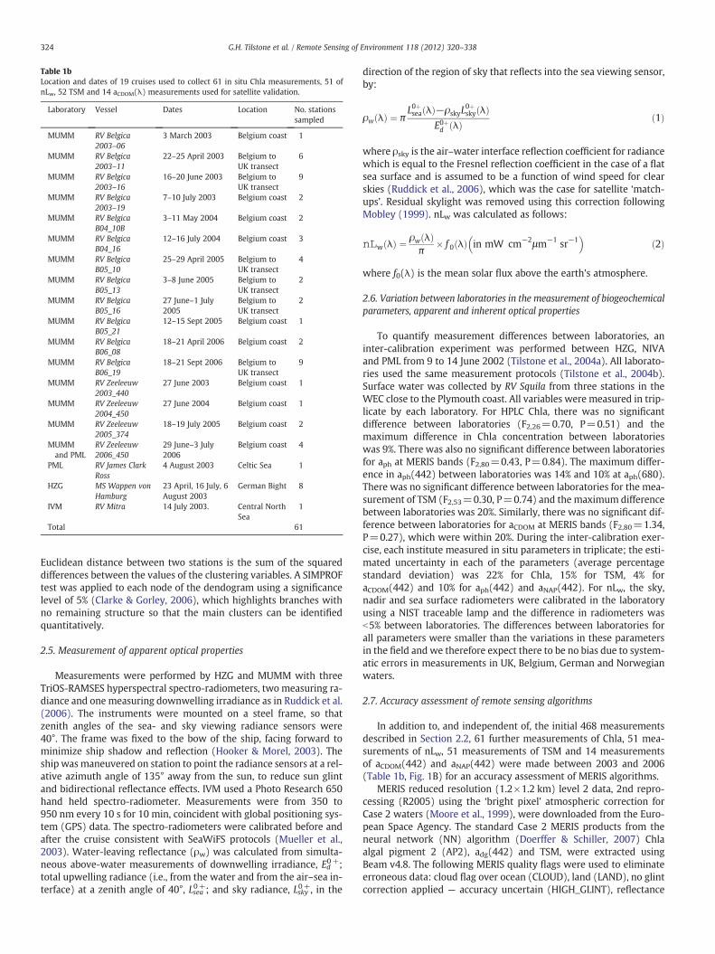
Table 1bLocation and dates of 19 cruises used to collect 61 in situ Chla measurements, 51 ofnLw, 52 TSM and 14 aCDOM(λ) measurements used for satellite validation.

Laboratory Vessel Dates Location No. stationssampled

MUMM RV Belgica2003–06

3 March 2003 Belgium coast 1


22–25 April 2003 Belgium toUK transect

6


16–20 June 2003 Belgium toUK transect

9


7–10 July 2003 Belgium coast 2

MUMM RV BelgicaB04_10B

3–11 May 2004 Belgium coast 2

MUMM RV BelgicaB04_16



25–29 April 2005 Belgium toUK transect

4


3–8 June 2005 Belgium toUK transect

2


27 June–1 July2005

Belgium toUK transect

2


12–15 Sept 2005 Belgium coast 1


18–21 April 2006 Belgium coast 2


18–21 Sept 2006 Belgium toUK transect

9

MUMM RV Zeeleeuw2003_440

27 June 2003 Belgium coast 1


27 June 2004 Belgium coast 1



MUMMand PML

RV Zeeleeuw2006_450

29 June–3 July2006

Belgium coast 4

PML RV James ClarkRoss

4 August 2003 Celtic Sea 1

HZG MS Wappen vonHamburg

23 April, 16 July, 6August 2003

German Bight 8

IVM RV Mitra 14 July 2003. Central NorthSea

1

Total 61


Euclidean distance between two stations is the sum of the squareddifferences between the values of the clustering variables. A SIMPROFtest was applied to each node of the dendogram using a significancelevel of 5% (Clarke & Gorley, 2006), which highlights branches withno remaining structure so that the main clusters can be identifiedquantitatively.

2.5. Measurement of apparent optical properties

Measurements were performed by HZG and MUMM with threeTriOS-RAMSES hyperspectral spectro-radiometers, two measuring ra-diance and one measuring downwelling irradiance as in Ruddick et al.(2006). The instruments were mounted on a steel frame, so thatzenith angles of the sea- and sky viewing radiance sensors were40°. The frame was fixed to the bow of the ship, facing forward tominimize ship shadow and reflection (Hooker & Morel, 2003). Theship was maneuvered on station to point the radiance sensors at a rel-ative azimuth angle of 135° away from the sun, to reduce sun glintand bidirectional reflectance effects. IVM used a Photo Research 650hand held spectro-radiometer. Measurements were from 350 to950 nm every 10 s for 10 min, coincident with global positioning sys-tem (GPS) data. The spectro-radiometers were calibrated before andafter the cruise consistent with SeaWiFS protocols (Mueller et al.,2003). Water-leaving reflectance (ρw) was calculated from simulta-neous above-water measurements of downwelling irradiance, Ed0+;total upwelling radiance (i.e., from the water and from the air–sea in-terface) at a zenith angle of 40°, Lsea0+; and sky radiance, Lsky0+, in the

direction of the region of sky that reflects into the sea viewing sensor,by:

ρw λð Þ ¼ πL0þsea λð Þ−ρskyL

0þsky λð Þ

E0þd λð Þ ð1Þ

where ρsky is the air–water interface reflection coefficient for radiancewhich is equal to the Fresnel reflection coefficient in the case of a flatsea surface and is assumed to be a function of wind speed for clearskies (Ruddick et al., 2006), which was the case for satellite ‘match-ups’. Residual skylight was removed using this correction followingMobley (1999). nLw was calculated as follows:

nLw λð Þ ¼ ρw λð Þπ

� f 0 λð Þ in mW cm−2μm−1 sr−1� �

ð2Þ

where f0(λ) is the mean solar flux above the earth's atmosphere.

2.6. Variation between laboratories in the measurement of biogeochemicalparameters, apparent and inherent optical properties

To quantify measurement differences between laboratories, aninter-calibration experiment was performed between HZG, NIVAand PML from 9 to 14 June 2002 (Tilstone et al., 2004a). All laborato-ries used the same measurement protocols (Tilstone et al., 2004b).Surface water was collected by RV Squila from three stations in theWEC close to the Plymouth coast. All variables were measured in trip-licate by each laboratory. For HPLC Chla, there was no significantdifference between laboratories (F2,26=0.70, P=0.51) and themaximum difference in Chla concentration between laboratorieswas 9%. There was also no significant difference between laboratoriesfor aph at MERIS bands (F2,80=0.43, P=0.84). The maximum differ-ence in aph(442) between laboratories was 14% and 10% at aph(680).There was no significant difference between laboratories for the mea-surement of TSM (F2,53=0.30, P=0.74) and the maximum differencebetween laboratories was 20%. Similarly, there was no significant dif-ference between laboratories for aCDOM at MERIS bands (F2,80=1.34,P=0.27), which were within 20%. During the inter-calibration exer-cise, each institute measured in situ parameters in triplicate; the esti-mated uncertainty in each of the parameters (average percentagestandard deviation) was 22% for Chla, 15% for TSM, 4% foraCDOM(442) and 10% for aph(442) and aNAP(442). For nLw, the sky,nadir and sea surface radiometers were calibrated in the laboratoryusing a NIST traceable lamp and the difference in radiometers wasb5% between laboratories. The differences between laboratories forall parameters were smaller than the variations in these parametersin the field and we therefore expect there to be no bias due to system-atic errors in measurements in UK, Belgium, German and Norwegianwaters.

2.7. Accuracy assessment of remote sensing algorithms

In addition to, and independent of, the initial 468 measurementsdescribed in Section 2.2, 61 further measurements of Chla, 51 mea-surements of nLw, 51 measurements of TSM and 14 measurementsof aCDOM(442) and aNAP(442) were made between 2003 and 2006(Table 1b, Fig. 1B) for an accuracy assessment of MERIS algorithms.

MERIS reduced resolution (1.2×1.2 km) level 2 data, 2nd repro-cessing (R2005) using the ‘bright pixel’ atmospheric correction forCase 2 waters (Moore et al., 1999), were downloaded from the Euro-pean Space Agency. The standard Case 2 MERIS products from theneural network (NN) algorithm (Doerffer & Schiller, 2007) Chlaalgal pigment 2 (AP2), adg(442) and TSM, were extracted usingBeam v4.8. The following MERIS quality flags were used to eliminateerroneous data: cloud flag over ocean (CLOUD), land (LAND), no glintcorrection applied — accuracy uncertain (HIGH_GLINT), reflectance


corrected for medium glint — accuracy maybe degraded (MEDIUM_-GLINT), highly absorbing aerosols (AODB), low sun angle (LOW_-SUN), low confidence flag for water leaving or surface reflectance(PCD1_13) and reflectance out of range (PCD_15). The MERIS L2products were extracted from a 3×3 pixel box, within ±0.5 h ofMERIS overpasses.

The semi-analytical algorithm HYDROPT (van der Woerd &Pasterkamp, 2008) was also used with the same R2005 MERIS data.HYDROPT comprises a forward model based on the HYDROLIGHT ra-diative transfer model (Mobley, 1994) and an inverse model based onleast-square fitting of the MERIS measured to modeled reflectance(Garver & Siegel, 1997; Maritorena et al., 2002). The forward modelgenerates a lookup table (LUT) of ρw as a function of the absorption(a) and scattering (b) properties and their constituent Chla, TSMand aCDOM, as follows:

ρw ¼ f a; b; θs; θv;φs;φv; Fresnel coef f icientwater�sky

� �ð3Þ

where f is a function, θs is the solar zenith angle, θv is the viewing ze-nith angle, φs is the solar azimuth angle, φv is the viewing azimuthangle and the Fresnel coefficient is the factor required for thewater–sky interface. The algorithm predicts remote sensing reflec-tance spectrum from a and b through knowledge of the sIOP for a par-ticular region as follows:

a λð Þ ¼ aw λð Þ þ aph � λð Þ � Chlaþ aNAP � λð Þ � TSM þ aCDOM � λð Þ� aCDOM 440ð Þ ð4Þ

b λð Þ ¼ bw λð Þ þ bp � λð Þ � TSM ð5Þ

where aw and bw are the absorption and scattering coefficients of purewater. HYDROPT was parameterized with median sIOP values(aCDOM*, aph*, aNAP*, and bp*) from the main cluster groups identifiedusing the methods described in Section 2.4. The HYDROPT algorithmwas run using MERIS data in bands 1 to 9, to estimate concentrationsof Chla, TSM and aCDOM(442). The scattering phase functions in theforward radiative transfer model were a uniform scattering functionfor pure water and the ‘San Diego harbor’ scattering phase functionfor TSM (Petzold, 1972). The algorithm retrieves the concentrationsfrom each sIOP type, by minimizing the chi square (χ2) difference be-tween observed MERIS and modeled reflectance spectra stored in theLUT (Mobley et al., 2005) at consecutive MERIS bands; 413, 442, 490,510, 560, 617, 665, 681 and 708, as follows:

χ2 ¼Xi¼m

i¼1

RRSiþ1MERIS−RiMERIS

� �− RRSiþ1Modelled−RiModelled

� �

σ

24

352

ð6Þ

where i is the band number, m is the band number minus 1 and σ isthe estimated standard error between bands based on Rast et al.(1999). The NN and HYDROPT use the same LUT. The only differencebetween them is in the bio-optical modeling and the use of differentsIOP datasets to retrieve the LUT values to match the MERIS and mod-eled reflectance. For HYDROPT, each sIOP type input is evaluated on apixel by pixel basis, and the sIOP type with the smallest χ2 differenceis selected. The sIOP data used in HYDROPT are not fixed and can becalibrated quickly using an ‘external’ data set, whereas the MERISNN algorithm requires extensive ‘internal’ calibration.

To evaluate algorithm performance we used the mean (M), stan-dard deviation (S), and root-mean square (RMS) of the differenceerror (D) between measured and satellite products at each stationas described in Campbell et al. (2002). The geometric mean andone-sigma range of the inverse transformed ratio between satelliteand measured values are given by M (Fmed), M–S (Fmin), M+S(Fmax) and were used as algorithm performance indices. The relative(RPD) and absolute percentage differences (APD) were calculated

following Antoine et al. (2008). We also used one way analysis of var-iance (ANOVA) to test for significant differences between in situ andsatellite products. Kolomogrov–Smirnov with Lilliefors tests wereused to check whether the distribution of in situ and satellite prod-ucts were normal. The ANOVA results are given as F1,108=x, P=ywhere F is the mean square to mean square error ratio, the sub-script numbers denote the degrees of freedom and P is the ANOVAcritical significance value.

3. Results

3.1. Variation in biogeochemical concentrations, inherent and specific-inherent optical properties in the North Sea

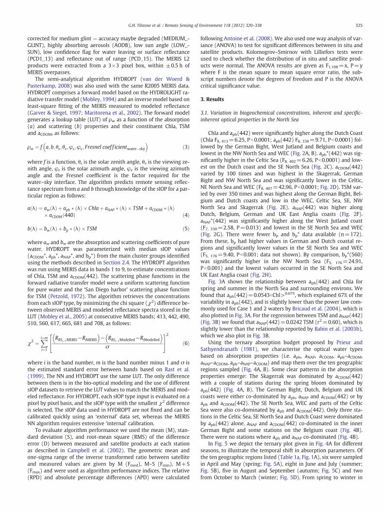
Chla and aph(442) were significantly higher along the Dutch Coast(Chla F8, 413=6.25, Pb0.0001; aph(442) F8, 338=9.71, Pb0.0001) fol-lowed by the German Bight, West Jutland and Belgium coasts andlowest in the NW North Sea and WEC (Fig. 2A, B). aph*(442) was sig-nificantly higher in the Celtic Sea (F8, 402=6.26, Pb0.0001) and low-est on the Dutch coast and the SE North Sea (Fig. 2C). aCDOM(442)varied by 100 times and was highest in the Skagerrak, GermanBight and NW North Sea and was significantly lower in the Celtic,NE North Sea and WEC (F8, 407=42.96, Pb0.0001; Fig. 2D). TSM var-ied by over 350 times and was highest along the German Bight, Bel-gium and Dutch coasts and low in the WEC, Celtic Sea, SE, NWNorth Sea and Skagerrak (Fig. 2E). aNAP(442) was higher alongDutch, Belgium, German and UK East Anglia coasts (Fig. 2F).aNAP*(442) was significantly higher along the West Jutland coast(F7, 330=2.58, P=0.013) and lowest in the SE North Sea and WEC(Fig. 2G). There were fewer bp and bp* data available (n=172).From these, bp had higher values in German and Dutch coastal re-gions and significantly lower values in the SE North Sea and WEC(F5, 176=9.40, Pb0.001; data not shown). By comparison, bp*(560)was significantly higher in the NW North Sea (F5, 176=24.91,Pb0.001) and the lowest values occurred in the SE North Sea andUK East Anglia coast (Fig. 2H).

Fig. 3A shows the relationship between aph(442) and Chla forspring and summer in the North Sea and surrounding environs. Wefound that aph(442)=0.0543bChl>0.675, which explained 67% of thevariability in aph(442), and is slightly lower than the power law com-monly used for Case 1 and 2 waters by Bricaud et al. (2004), which isalso plotted in Fig. 3A. For the regression between TSM and aNAP(442)(Fig. 3B) we found that aNAP(442)=0.0242 TSM (r2=0.60), which isslightly lower than the relationship reported by Babin et al. (2003b),which we also plot in Fig. 3B.

Using the ternary absorption budget proposed by Prieur andSathyendranath (1981), we characterise the optical water typesbased on absorption properties (i.e. aph, aNAP, aCDOM, aph–aCDOM,aNAP–aCDOM, aph–aNAP–aCDOM) and map them over the ten geographicregions sampled (Fig. 4A, B). Some clear patterns in the absorptionproperties emerge: The Skagerrak was dominated by aCDOM(442)with a couple of stations during the spring bloom dominated byaph(442) (Fig. 4A, B). The German Bight, Dutch, Belgium and UKcoasts were either co-dominated by aph, aNAP and aCDOM(442) or byaph and aCDOM(442). The SE North Sea, WEC and parts of the CelticSea were also co-dominated by aph and aCDOM(442). Only three sta-tions in the Celtic Sea, SE North Sea and Dutch Coast were dominatedby aph(442) alone. aNAP and aCDOM(442) co-dominated in the innerGerman Bight and some stations on the Belgium coast (Fig. 4B).There were no stations where aph and aNAP co-dominated (Fig. 4B).

In Fig. 5 we depict the ternary plot given in Fig. 4A for differentseasons, to illustrate the temporal shift in absorption parameters. Ofthe ten geographic regions listed (Table 1a, Fig. 1A), six were sampledin April and May (spring; Fig. 5A), eight in June and July (summer;Fig. 5B), five in August and September (autumn; Fig. 5C) and twofrom October to March (winter; Fig. 5D). From spring to winter in

A

Chla (mgm-3)0.1 1 10

E

TSM (gm-3)0.1 1 10

C

aph* (mgm-2)0.01 0.1

G

aNAP* (g m-2)0.001 0.01 0.1

B

aph (m-1)

0.001 0.01 0.1 1

F

aNAP (m-1)

0.001 0.01 0.1 1

D

aCDOM (m-1)

0.01 0.1 1

H

bp* (m2 g TSM-1)

0.01 0.1 1

SkagerrakNW North Sea

East AngliaSE North Sea

German BightDutch CoastWest Jutland

Belgium CoastWEC

Celtic Sea




Belgium CoastWEC

Celtic Sea




Belgium CoastWEC

Celtic Sea




Belgium CoastWEC

Celtic Sea

Fig. 2. Box plots of (A) Chla, (B) aph(442), (C) aph*(442), (D) aCDOM(442), (E) TSM, (F) aNAP(442), (G) aNAP*(442), (H) bp*(560) for the 10 geographic regions given in Figure 1. Theboundary of the box closest to zero indicates the 25th percentile, the solid line within the box is the median, the dashed line is the mean and the boundary of the box farthest fromzero indicates the 75th percentile. The error bars above and below the box indicate the 90th and 10th percentiles and the points beyond the error bars are outliers.


the German Bight aCDOM(442) generally dominated but the relativecontributions of aph and aNAP shifted with season so that in springmore stations were dominated by aph(442), whereas in autumn andwinter the stations sampled had a higher proportion of aNAP(442).From April to September the WEC stations were either highaph(442) and low aCDOM(442) or low aph and high aCDOM (Fig. 5a, B,C) reflecting the influence of the Atlantic inflow from the Celtic Seaor the freshwater outflow from River Tamar. By winter, the WEC

samples were dominated by aCDOM(442) alone (Fig. 5D). The Dutchcoast samples tended to have higher aph(442) in April and May(Fig. 5A) but higher aCDOM(442) in August and September (Fig. 5C).The Skagerak samples remained high aCDOM, low aph and aNAP fromApril to September (Fig. 5A, B, C).

To compare the distribution of IOP with sIOP we employed clusteranalysis on coincident measurements of aCDOM(442), aph*(442) andaNAP*(442). The analysis segregated three principal clusters

image of Fig.�2

A

Chla (mg m-3)

0.1 1 10 100

a ph

(442

) (m

-1)

0.001

0.01

0.1

1

10

B

0.1 1 10 100

a NA

P (4

42)

(m-1

)

0.001

0.01

0.1

1

10

TSM (g m-3)

Fig. 3. Scatterplots of (A) aph(442) as a function of Chla; solid line regression from ourdata, dotted line Bricaud et al. (2004) regression, (B) aNAP(442) as a function of TSM;solid line regression from our data, dotted line Babin et al. (2003) regression. Symbolsas in Figure 1, except NW North Sea, which is hexagon.

A

0.0 0.1 0.2 0.3 0.4 0.5 0.6 0.7 0.8 0.9 1.00.0

0.1

0.2

0.3

0.4

0.5

0.6

0.7

0.8

0.9

1.00.0

0.1

0.2

0.3

0.4

0.5

0.6

0.7

0.8

0.9

1.0

B

C

aNAP (λ)

aph (λ)aCDOM (λ)

Fig. 4. Ternary plot showing the relative contribution of (A) aph(442), aNAP(442) andaCDOM(442) to total absorption in the North Sea. The different Symbols represent thedifferent geographic regions illustrated in Figure 1, except NW North Sea, which ishexagon. (B) The distribution of the main groups optical types in the North Sea givenin (A) shown in the inset as aph (cross), aNAP (circle), aCDOM (plus), aph–aCDOM (dia-mond), aCDOM–aNAP (inverted triangle), aph–aCDOM–aNAP (cross). (C) Geographic distri-bution of main groupings from cluster analysis on aph*(442), aNAP*(442) andaCDOM(442). Cluster 1 is diamond, Cluster 2 is cross, Cluster 3 is circle.


(Fig. 5C). The largest (Cluster 2, n=161) grouped stations with lowaph*, high aNAP* and aCDOM, which also had high bp* (median valuesaph*(442) 0.029±0.012 mg m−2, aNAP*(442) 0.041±0.023 g m−2,aCDOM(442) 0.367±0.287 m−1, bp* 0.36±0.31 m2 g TSM−1; Fig. 6)from the Belgium, Danish and German coasts. The second largest(Cluster 3, n=137) grouped stations with medium aph*, aNAP* andaCDOM which had lower bp* (median aph*(442) 0.041±0.022 mgm−2,aNAP*(442) 0.018±0.013 g m−2, aCDOM(442) 0.227±0.164 m−1, bp*0.28±0.20 m2 g TSM−1; Fig. 6) from the Southern Bight betweenthe Belgium and UK coasts, NE North Sea, WEC and Skagerrak. Thesmallest cluster (Cluster 1, n=18) grouped stations with high aph*,low aNAP* and aCDOM from the WEC, Celtic and SE North Seas (medianaph*(442) 0.047±0.147 mgm−2, aNAP*(442) 0.012±0.013 g m−2,aCDOM(442) 0.062±0.073 m−1, too few bp* data, default value used;Fig. 6).

To assess the influence of river discharge in the coastal zone on theabsorption and specific-absorption properties we plot the relation-ships between aCDOM(442) and aNAP(442) and salinity (Fig. 7A, B) asa function of the optical types from the ternary absorption budgetgiven in Fig. 4B. We also plot aCDOM(442) and aNAP*(442) against sa-linity as a function of the main sIOP groups from the cluster analysis

(Fig. 7C, D). For aCDOM(442) and salinity we observed two main re-gressions; one for aCDOM and aph–aCDOM type waters, whereaCDOM(442)=−0.020×Salinity — 0.91 (r2=0.24, P=0.0002;dashed line in Fig. 7A) which corresponds to the relationship ob-served for sIOP Cluster 3 (aCDOM(442)=−0.015×Salinity — 0.72,r2=0.35, Pb0.0001; dashed line in Fig. 7C). The other aCDOM(442)-sa-linity regression was for aNAP–aCDOM and aNAP–aph–aCDOM type waterswhere aCDOM(442)=−0.066×Salinity+2.35 (r2=0.93, Pb0.0001;solid line in Fig. 7A) which corresponds to the relationship observedfor sIOP Cluster 2 where aCDOM(442)=−0.058×Salinity+2.12,(r2=0.70; solid line in Fig. 7C). For aNAP(442) and salinity therewas one significant regression for aNAP–aCDOM and aNAP–aph–aCDOM

A

0.0 0.1 0.2 0.3 0.4 0.5 0.6 0.7 0.8 0.9 1.00.0

0.1

0.2

0.3

0.4

0.5

0.6

0.7

0.8

0.9

1.00.0

0.1

0.2

0.3

0.4

0.5

0.6

0.7

0.8

0.9

1.0

B

0.0 0.1 0.2 0.3 0.4 0.5 0.6 0.7 0.8 0.9 1.00.0

0.1

0.2

0.3

0.4

0.5

0.6

0.7

0.8

0.9

1.00.0

0.1

0.2

0.3

0.4

0.5

0.6

0.7

0.8

0.9

1.0

C

aNAP (442) (m-1)

0.0 0.1 0.2 0.3 0.4 0.5 0.6 0.7 0.8 0.9 1.00.0

0.1

0.2

0.3

0.4

0.5

0.6

0.7

0.8

0.9

1.00.0

0.1

0.2

0.3

0.4

0.5

0.6

0.7

0.8

0.9

1.0

D

0.0 0.1 0.2 0.3 0.4 0.5 0.6 0.7 0.8 0.9 1.00.0

0.1

0.2

0.3

0.4

0.5

0.6

0.7

0.8

0.9

1.00.0

0.1

0.2

0.3

0.4

0.5

0.6

0.7

0.8

0.9

1.0

aNAP (442) (m-1)

aph (442) (m-1)

aCDOM (442) (m-1)aCDOM (442) (m-1)aph (442) (m-1)

aNAP (442) (m-1) aNAP (442) (m-1)

aCDOM (442) (m-1)

aph (442) (m-1)aCDOM (442) (m-1)

aph (442) (m-1)

Fig. 5. Ternary plots showing the temporal change in aph(442), aNAP(442) and aCDOM(442) during (A) April–May, (B) June–July, (C) August–September, (D) October–March. Symbols asin Figure 1, except NW North Sea, which is hexagon.


type waters, where aNAP(442)=−0.042×Salinity+1.58 (r2=0.49,Pb0.0001; solid line in Fig. 7B), illustrating that low aNAP(442) is as-sociated with higher salinity stations influenced by Atlantic waterand high aNAP(442) is associated with stations in coastal waters influ-enced by river runoff. The other regression plotted in Fig. 7B is for theaCDOM and aph–aCDOM type waters but was not significant sinceaNAP(442) was consistently low with varying salinity. By comparison,the regression between aNAP*(442) and salinity explained a lowerpercentage of variance and Clusters 2 and 3 had similar slopes(Cluster 3 aNAP*(442)=−0.0011×Salinity+0.053, r2=0.12; Cluster2 aNAP*(442)=−0.0013×Salinity+0.08, r2=0.05, Fig. 7D), illustrat-ing a weaker link between aNAP*(442) and river discharge. There wasno significant regression between aph(442) and aph*(442) and salinityfor any of the Cluster groups (data not shown).

3.2. Accuracy assessment of MERIS derived products

The median values in sIOP at MERIS bands 1–9 from the threegroups characterized by the cluster analysis (Fig. 6) were used to pa-rameterize the semi-analytical algorithm HYDROPT. There were fewbp*(555) data available for Cluster 1 to be statistically representativeof this group, so the default reference value was used. We then usedthe 61 in situ match-up points for Chla, 51 for nLw, 51 for TSM, and14 for aCDOM(442) and aNAP(442) to assess the accuracy of both stan-dard MERIS ocean colour and the newly parameterized HYDROPT al-gorithm (Figs. 8, 9). The majority of the stations were from theBelgium coast, the others were from the German Bight, NW NorthSea and Celtic Sea (Table 1b, Fig. 1B).

Firstly we assessed the 2nd reprocessing of MERIS nLw against insitu nLw to evaluate the accuracy of the satellite radiometers and at-mospheric correction (Fig. 8). The range in in situ nLw(442) at the val-idation stations was 0.2 to 0.54 mW cm−2 μm−1 sr−1. Generally theRMS, bias, RPD and APD decreased and Fmed, Fmin, Fmax increasedfrom nLw(412) to nLw(560) (Table 2), indicating that MERIS is moreaccurate in the North Sea at 560 nm than at 412, 443 and 490 nm.The APD for nLw(665) was similar to that in the blue, though theRPD and RMS were lower (Table 2). The regression slope was closerto 1 for MERIS nLw(442) compared to nLw(560) and nLw(665), butthe offset was higher (Fig. 8).

For MERIS Chla algorithms the log10-RMS was 0.26, indicatingagreement with in situ values within a factor of 2 (Table 2). Therange in Chla at the validation stations was 0.26 to 27.57 mg m−3

and the geometric means (Fmed, Fmin, Fmax) were close to 1 for bothAP2 and HYDROPT, indicating a high level of accuracy over therange tested. The random error (S) and bias (M and RPD) of both al-gorithms was low (Sb0.3, Mb0.1), though MERIS AP2 had a slightlyhigher APD since it tended to under-estimate Chla at valuesb5 mg m−3 (Table 2, Fig. 9A). HYDROPT Chla exhibited a smallerbias indicated by the lower RMS (Table 2, Fig. 9B). As a consequence,in satellite images from 22 April 2003, MERIS AP2 gave higher Chlavalues during the spring bloom in the Celtic Sea, SE, NW North Sea,Skagerrak and WEC compared to HYDROPT, but lower values in con-tinental European coastal areas (Fig. 10A, B).

In situ TSM at the match-up stations varied between 1.01 and95.22 g m−3 and at least 65% of the stations had TSM >3.0 g m−3.We found that for the North Sea, MERIS and HYDROPT TSM had a

Cluster 2

a CD

OM

* (u

nit l

ess)

0.0

0.5

1.0

1.5

2.0

2.5

Cluster 3

Wavelength (nm)400 450 500 550 600 650

a CD

OM

* (u

nit l

ess)

0.0

0.5

1.0

1.5

2.0

2.5

Cluster 1

a CD

OM

* (u

nit l

ess)

0.0

0.5

1.0

1.5

2.0

2.5

Cluster 2

a ph*

(m

2 mg

Chl

a-1)

0.00

0.02

0.04

0.06

0.08

0.10

0.12

0.14

0.16

0.18

Cluster 3

Wavelength (nm)400 450 500 550 600 650

a ph*

(m

2 mg

Chl

a-1)

0.00

0.02

0.04

0.06

0.08

0.10

0.12

0.14

0.16

0.18

Cluster 1

a ph*

(m

2 mg

Chl

a-1)

0.00

0.02

0.04

0.06

0.08

0.10

0.12

0.14

0.16

0.18

Cluster 2

0.00

0.05

0.10

0.15

0.20

Cluster 3

Wavelength (nm)400 450 500 550 600 650

0.00

0.05

0.10

0.15

0.20

Cluster 1

a NA

P* (

m2 g

TSM

-1)

0.00

0.05

0.10

0.15

0.20

Cluster 2

0.0

0.2

0.4

0.6

0.8

1.0

1.2

Cluster 3

Wavelength (nm)400 450 500 550 600 650

0.0

0.2

0.4

0.6

0.8

1.0

1.2

Cluster 1

b p*

(m2 g

TSM

-1)

0.0

0.2

0.4

0.6

0.8

1.0

1.2

a NA

P* (

m2 g

TSM

-1)

a NA

P* (

m2 g

TSM

-1)

b p*

(m2 g

TSM

-1)

b p*

(m2 g

TSM

-1)

Fig. 6. Relationship between salinity and (a.) aCDOM(442) and (b.) aNAP(442) with the absorption types shown in Figure 4b. In (a.) and (b.) solid line is regression for aNAP-aCDOM and aNAP-aph-aCDOM type waters and dashed line is for aCDOMand aph-aCDOM type waters. Relationship between salinity and (c.) aCDOM(442) and (d.) aNAP*(442) with the sIOP cluster groups shown in Figure 4c. In (c.) and (d.) solid line is regression for cluster 2 sIOP type and dashed line is for cluster 3sIOP type.

329G.H.Tilstone

etal./

Remote

SensingofEnvironm

ent118

(2012)320

–338

A

a CD

OM

(m

-1)

a NA

P (m

-1)

a NA

P* (g

m-2

)

a CD

OM

(m

-1)

0.0

0.2

0.4

0.6

0.8

1.0

1.2

1.4

1.6 B

0.0

0.5

1.0

1.5

2.0

C

Salinity

0.0

0.2

0.4

0.6

0.8

1.0

1.2

1.4

1.6 D

Salinity

10 15 20 25 30 35 4010 15 20 25 30 35 40

10 15 20 25 30 35 4010 15 20 25 30 35 400.00

0.02

0.04

0.06

0.08

0.10

0.12

0.14

0.16

0.18

Fig. 7. Range and median (thick line in each plot) of aph*(λ), aNAP*(λ), aCDOM(λ normalized to 442) and bp*(λ) for Cluster 1, 2 and 3, used to parameterize HYDROPT. For bp*(λ)Cluster 1, the median is from the original reference value given in van der Woerd and Pasterkamp (2008).


similar log10-RMS, but MERIS had a lower S. The Fmed was closer to 1for HYDROPT, but the Fmax was closer to 1 for MERIS (Table 2, Fig. 9C,D), which resulted in a regression slope closer to 1 for HYDROPT com-pared to MERIS TSM. For HYDROPT RPD and APDwere higher due to ahigher scatter at lower TSM values (Fig. 9D). This resulted in a lowerestimate in HYDROPT TSM values in the Celtic Sea, WEC and in Nor-wegian waters in April 2003, compared to MERIS TSM, but a higherestimate in the Southern Bight, Belgium, Dutch and UK coastal waters(Fig. 10C, D). TSM concentrations were similar for both algorithmsalong the German Bight.

The range in aCDOM(442) and adg(442) at the validation stationswas 0.01 to 0.673 m−1 and 0.027 to 1.71 m−1, respectively. Com-pared to MERIS adg(442) algorithm, the RMS values were lower forHYDROPT aCDOM(442) and indicate an agreement with in situ valuesof ~1.5, whereas the difference for MERIS adg(442) was a factor of ~3(Table 2). The random error (S), bias (M and RPD), APD and inter-cept for the HYDROPT algorithm were also lower, Fmed and Fmin

values and slope were closer to 1, which also shows a closer agree-ment between in situ and HYDROPT aCDOM(442) compared withMERIS adg(442) (Table 2, Fig. 9E, F). There was a slight tendencyfor HYDROPT to over-estimate aCDOM(442) at high values whenCluster 2 was implemented (Fig. 9F). For MERIS adg(442) therewas a consistent under-estimation when values were b0.06 m−1.The spatial pattern in MERIS adg(442) and HYDROPT aCDOM(442)satellite maps of 22 April 2003 was similar, but the values in someareas were very different (Fig. 10E, F). For example, in the CelticSea, SE North Sea and West Jutland Belgium and Dutch coasts,MERIS adg(442) was an order of magnitude higher than HYDROPTaCDOM(442).

4. Discussion

4.1. Variation in inherent and specific-inherent optical properties of theNorth Sea

A comparison of the mean absorption properties of the North Seafrom our data with historic studies is given in Table 3. There is highsimilarity in our aph(442) and aph*(442) with those from previousstudies indicating that the 468 data we collected is representative ofthe variability in IOP sIOP of the North Sea. Our mean aph(442) forthe North Sea was 0.16 m−1 and similar to that of Babin et al.(2003b) and Vantrepotte et al. (2007). Our mean aph*(442) was0.044 m2 mg Chla−1 and similar to the values given in Staehr et al.(2004) and Tilstone et al. (2005). The aCDOM(442) values we reportare also similar to those given for the North Sea (Astoreca et al.,2009), English Channel (Vantrepotte et al., 2007) and other UK coast-al areas (Foden et al., 2008), but lower than some data sets for theBaltic Sea and Skagerrak. When only data from coastal regions wereincluded in our analysis, aCDOM(442) was significantly lower on theEast Anglia, UK and Belgium coasts (mean~0.2 m−1; F5, 346=2.32,P=0.043), whereas it was higher and similar along the GermanBight (mean~0.42 m−1), Skagerrak (~0.38 m−1), Dutch coast(~0.34 m−1) and West Jutland (~0.31 m−1). We found ouraNAP(442) values, to be slightly higher than those values previouslyreported for the North Sea, English Channel and Irish Sea, 50% lessthan those values reported for other European estuarine and coastalwaters (Table 3), but within a similar range to those given in Babinet al. (2003a) and Ferrari et al. (2003). The higher aNAP(442) is dueto high values along the Dutch coast, resulting from a high organic

A) 442nm

0.0 0.2 0.4 0.6 0.8 1.00.0

0.2

0.4

0.6

0.8

1.0

B) 560 nm

0.0 0.2 0.4 0.6 0.80.0

0.2

0.4

0.6

0.8

Y = 1.15X + 0.25, r2 = 0.37.

Y = 0.73X - 0.05, r2 = 0.82.

C) 665 nm

0.0 0.1 0.2 0.3 0.40.0

0.1

0.2

0.3

0.4

Y = 0.62X - 0.02, r2 = 0.76.

in situ nLw (mW cm-2 μm-1 sr-1)

ME

RIS

nL

w (

mW

cm

-2 μ

m-1

sr-1

)

Fig. 8. Comparison of in situ nLw with MERIS nLw for (A) 442, (B) 560 and (C) 665 nm.Solid line is 1:1. The regression equation is given in the inset.


content of the TSM in the Wadden Sea (Hommersom et al., 2009),probably resulting from high Chla in these waters and agriculturalrunoff to the coast. For aNAP*(442), few values have been reportedfor the North Sea (Table 3). We found that aNAP*(442) was significant-ly higher on the West Jutland coast due to comparatively low TSM

(Fig. 2G), indicating high organic detritus in these waters, possiblydue to the soil type and agricultural runoff on the West coast of Den-mark as suggested by Stedmon et al. (2000). A detailed analysis of bpfor this area has already been conducted by Babin et al. (2003a), whoshowed that light scattering at 555 nm was principally due to min-erals with a low clay and silt content that occur along the Europeanshelf. Babin et al. (2003a) reported mean bp*(559) of 0.54 m2g−1

for coastal waters of the North Sea. Our mean value of 0.44 m2g−1

for the North Sea andWEC is slightly lower than this due to the inclu-sion of more stations in coastal waters and possibly due to the differ-ence in pore size of filters used. In our study, the same protocols wereused by each laboratory and inter-calibration exercises showed thatthere was no significant bias in measurements between laboratories.The 95% confidence interval of aph*(442), aNAP*(442), bp*(560) andaCDOM(442) were low and did not produce significant deviationsfrom the mean, indicating that the error associated with this dataset was low. In addition, we confirmed that our IOP and sIOP valueswere typical of the North Sea by comparing with previous literaturevalues (Table 3).

The power law commonly used for aph as a function of Chla isaph(440)=0.0654(TChla)0.728 (Bricaud et al., 2004). Using the 392Chla data points from this study, we used the Bricaud et al. (2004) re-lationship and our model to calculate aph(440) and found a significantdifference between models (F1, 569=17.76, Pb0.0001). The Bricaudet al. (2004) data was predominantly collected in Case 1 waterswith some stations in coastal waters, whereas our data was mostlyfrom Case 2 waters, where the difference in the underwater light re-gime due to higher TSM and aCDOM may modify the aph–Chla relation-ship. For aNAP(442) and TSMwe found that aNAP(442)=0.0242×TSM(r2=0.60). Similarly Bowers and Mitchelson-Jacob (1996) reportedthat aNAP(443)=0.0235×TSM. The relationship reported by Babinet al. (2003b) was slightly higher aNAP(443)=0.031×TSM, probablybecause their data included more open ocean stations and they useda smaller filter pore size 0.2 μm. For the 343 TSM data collected dur-ing this study we used each model to re-calculate aNAP(443) andfound no difference between our model and those of Bowers andMitchelson-Jacob (1996) and Babin et al. (2003b) (F2, 1028=2.41,P=0.090), suggesting that any of these relationships could be usedwith the same relative accuracy to derive TSM from satellite.

The ternary plot of absorption (Fig. 4A), indicates that the NorthSea is principally dominated by aCDOM(442) or co-dominated byaCDOM(442) and aph(442). Less than 1% of the stations were dominat-ed by aNAP(442) which represent waters with a high organic TSMcontent that absorb light. However, aNAP(442) is a poor proxy for clas-sifying inorganic sediments which have little capacity for absorbinglight. Alternatively, Siegel et al. (2005b) used the single scatter ap-proximation and the absorption of phytoplankton and CDOM as a ter-nary plot to assess the contribution of these to the diffuse attenuationcoefficient, kd(λ). On a global basis, they found that the contributionof bbp(λ) to kd(λ) was b10%, Chla contributed 40% and adg accountedfor 50% of the variability. Scattering and backscattering properties areas important to ocean colour as absorption properties, but in the ab-sence of a comprehensive bp(λ) and bbp(λ) data sets, we employedcluster analysis on specific-absorption properties to assess the relat-edness in these properties between stations. This approach is alsocomplementary with the optical water types original identified byPrieur and Sathyendranath (1981). From the principal clusters identi-fied, there were broadly three main groups which radiated in bandsfrom the coast. Cluster 1 had low aNAP*(442), aCDOM(442) and highaph*(442), occupying open ocean stations. Cluster 2 with lowaph*(442), high aNAP*(442) and aCDOM(442) occurred close to thecoast. Cluster 3 occupied stations between the coast and open oceanand in the Skagerak with medium aph*(442), aNAP*(442) andaCDOM(442) (Fig. 4C). The Norwegian coast is influenced by a deep in-flow of Atlantic water and a surface outflow of Baltic water, which re-sults in high aCDOM along the southern Norwegian (Høkedal et al.,

A

In Situ Chla (mgm-3)

ME

RIS

AP2

(m

g m

-3)

0.1

1

10

100MERIS AP2 Chlalog(Y) = log(x)0.69 + 0.078; r2 = 0.51; N = 61.

B

In Situ Chla (mgm-3)

0.1 1 10 100 0.1 1 10 100

0.1 1 10 100 0.1 1 10 100

HY

DR

OPT

Chl

a (m

g m

-3)

0.1

1

10

100HYDROPT sIOP Chlalog(Y) = log(x)0.84 + 0.02; r2 = 0.88; N = 61.

C

In Situ TSM (g m-3)

ME

RIS

TSM

(g

m-3

)

0.1

1

10

100

D

In Situ TSM (g m-3)

HY

DR

OPT

TSM

(g

m-3

)

0.1

1

10

100 HYDROPT sIOP TSMlog(Y) = log(x)0.94 - 0.10; r2 = 0.67; N = 52.

MERIS TSMlog(Y) = log(x)0.87 - 0.11; r2 = 0.74; N = 52.

HYDROPT sIOP aCDOM

log(Y) = log(x)0.90 - 0.09; r2 = 0.70; N = 15.

In Situ aCDOM (442) (m-1)

HY

DR

OPT

aC

DO

M (

442)

(m

-1)

0.001

0.01

0.1

1

10MERIS adg

log(Y) = log(x)0.87 - 0.32; r2 = 0.43; N = 15.

In Situ adg (442) (m-1)

0.001 0.01 0.1 1 100.001 0.01 0.1 1 10

ME

RIS

adg

(44

2) (

m-1

)

0.001

0.01

0.1

1

10E F

Fig. 9. Comparison of in situ and satellite derived (A)MERIS Algal Pigment 2 Chla, (B) HYDROPT sIOP Chla, (C)MERIS TSM (D) HYDROPT sIOP TSM, (E) MERIS adg(442) and (F) HYDROPTsIOP aCDOM(442). Faint dotted lines are the 1:1 line, upper and lower 20% quartiles. In (B), (D) and (F) Cluster 1 is diamond, Cluster 2 is cross, Cluster 3 is circle. The regression equation isgiven in the inset.


2005) and Danish coasts (Stedmon et al., 2000). The east–west sepa-ration in sIOP characterised by Clusters 2 and 3 therefore seems to beby stations influenced by riverine run-off from continental Europeand UK coasts (Cluster 2) and those influenced by Baltic Sea andshelf areas (Cluster 3). Though the European Continental coastal

margin is influenced by high aCDOM from the fresh water outflow ofthe Elbe, Rhine and Scheldt rivers (Warnock et al., 1999), our analysissuggests that these stations are also associated by high aNAP*(442),which differentiates stations further offshore with lower aNAP*(442)values. There were similarities between the cluster analysis and the

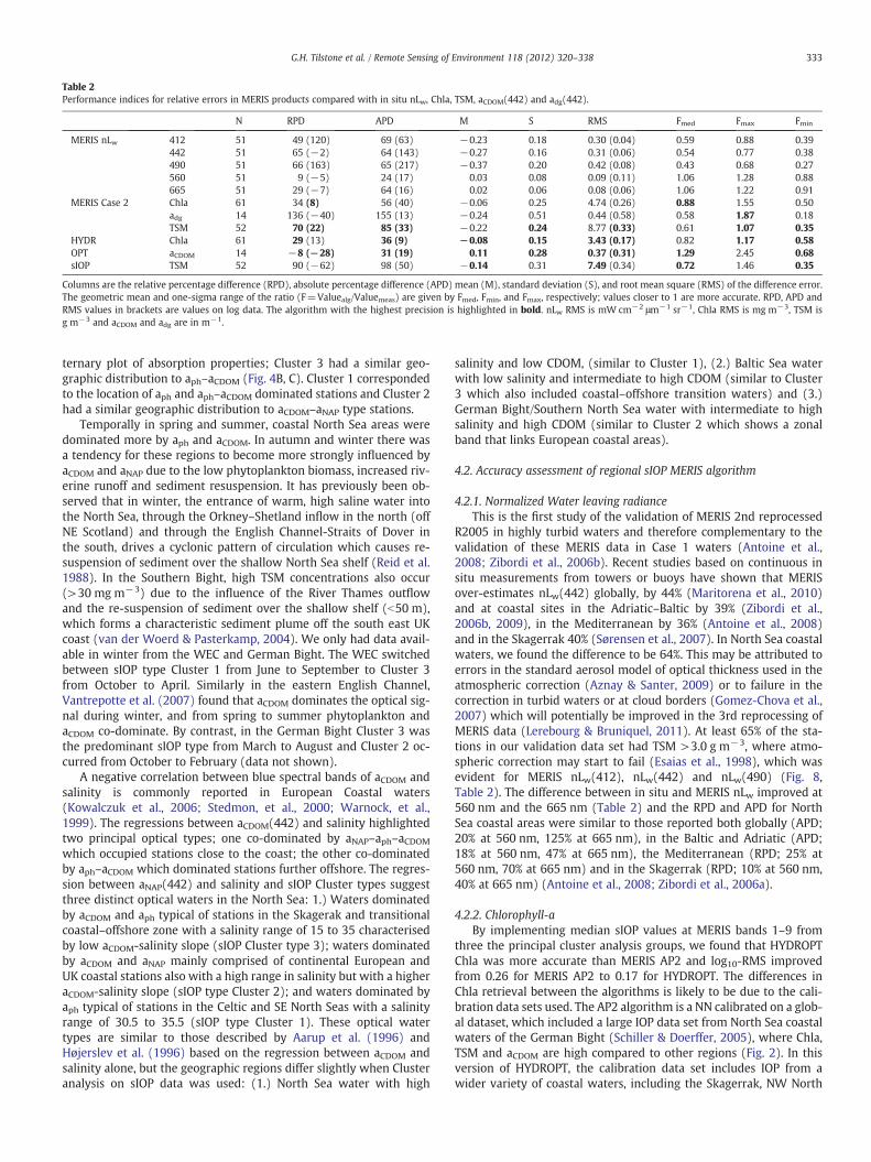
Table 2Performance indices for relative errors in MERIS products compared with in situ nLw, Chla, TSM, aCDOM(442) and adg(442).

N RPD APD M S RMS Fmed Fmax Fmin

MERIS nLw 412 51 49 (120) 69 (63) −0.23 0.18 0.30 (0.04) 0.59 0.88 0.39442 51 65 (−2) 64 (143) −0.27 0.16 0.31 (0.06) 0.54 0.77 0.38490 51 66 (163) 65 (217) −0.37 0.20 0.42 (0.08) 0.43 0.68 0.27560 51 9 (−5) 24 (17) 0.03 0.08 0.09 (0.11) 1.06 1.28 0.88665 51 29 (−7) 64 (16) 0.02 0.06 0.08 (0.06) 1.06 1.22 0.91

MERIS Case 2 Chla 61 34 (8) 56 (40) −0.06 0.25 4.74 (0.26) 0.88 1.55 0.50adg 14 136 (−40) 155 (13) −0.24 0.51 0.44 (0.58) 0.58 1.87 0.18TSM 52 70 (22) 85 (33) −0.22 0.24 8.77 (0.33) 0.61 1.07 0.35

HYDR Chla 61 29 (13) 36 (9) −0.08 0.15 3.43 (0.17) 0.82 1.17 0.58OPT aCDOM 14 −8 (−28) 31 (19) 0.11 0.28 0.37 (0.31) 1.29 2.45 0.68sIOP TSM 52 90 (−62) 98 (50) −0.14 0.31 7.49 (0.34) 0.72 1.46 0.35

Columns are the relative percentage difference (RPD), absolute percentage difference (APD) mean (M), standard deviation (S), and root mean square (RMS) of the difference error.The geometric mean and one-sigma range of the ratio (F=Valuealg/Valuemeas) are given by Fmed, Fmin, and Fmax, respectively; values closer to 1 are more accurate. RPD, APD andRMS values in brackets are values on log data. The algorithm with the highest precision is highlighted in bold. nLw RMS is mW cm−2 μm−1 sr−1, Chla RMS is mg m−3, TSM isg m−3 and aCDOM and adg are in m−1.


ternary plot of absorption properties; Cluster 3 had a similar geo-graphic distribution to aph–aCDOM (Fig. 4B, C). Cluster 1 correspondedto the location of aph and aph–aCDOM dominated stations and Cluster 2had a similar geographic distribution to aCDOM–aNAP type stations.

Temporally in spring and summer, coastal North Sea areas weredominated more by aph and aCDOM. In autumn and winter there wasa tendency for these regions to become more strongly influenced byaCDOM and aNAP due to the low phytoplankton biomass, increased riv-erine runoff and sediment resuspension. It has previously been ob-served that in winter, the entrance of warm, high saline water intothe North Sea, through the Orkney–Shetland inflow in the north (offNE Scotland) and through the English Channel-Straits of Dover inthe south, drives a cyclonic pattern of circulation which causes re-suspension of sediment over the shallow North Sea shelf (Reid et al.1988). In the Southern Bight, high TSM concentrations also occur(>30 mg m−3) due to the influence of the River Thames outflowand the re-suspension of sediment over the shallow shelf (b50 m),which forms a characteristic sediment plume off the south east UKcoast (van der Woerd & Pasterkamp, 2004). We only had data avail-able in winter from the WEC and German Bight. The WEC switchedbetween sIOP type Cluster 1 from June to September to Cluster 3from October to April. Similarly in the eastern English Channel,Vantrepotte et al. (2007) found that aCDOM dominates the optical sig-nal during winter, and from spring to summer phytoplankton andaCDOM co-dominate. By contrast, in the German Bight Cluster 3 wasthe predominant sIOP type from March to August and Cluster 2 oc-curred from October to February (data not shown).

A negative correlation between blue spectral bands of aCDOM andsalinity is commonly reported in European Coastal waters(Kowalczuk et al., 2006; Stedmon, et al., 2000; Warnock, et al.,1999). The regressions between aCDOM(442) and salinity highlightedtwo principal optical types; one co-dominated by aNAP–aph–aCDOMwhich occupied stations close to the coast; the other co-dominatedby aph–aCDOM which dominated stations further offshore. The regres-sion between aNAP(442) and salinity and sIOP Cluster types suggestthree distinct optical waters in the North Sea: 1.) Waters dominatedby aCDOM and aph typical of stations in the Skagerak and transitionalcoastal–offshore zone with a salinity range of 15 to 35 characterisedby low aCDOM-salinity slope (sIOP Cluster type 3); waters dominatedby aCDOM and aNAP mainly comprised of continental European andUK coastal stations also with a high range in salinity but with a higheraCDOM-salinity slope (sIOP type Cluster 2); and waters dominated byaph typical of stations in the Celtic and SE North Seas with a salinityrange of 30.5 to 35.5 (sIOP type Cluster 1). These optical watertypes are similar to those described by Aarup et al. (1996) andHøjerslev et al. (1996) based on the regression between aCDOM andsalinity alone, but the geographic regions differ slightly when Clusteranalysis on sIOP data was used: (1.) North Sea water with high

salinity and low CDOM, (similar to Cluster 1), (2.) Baltic Sea waterwith low salinity and intermediate to high CDOM (similar to Cluster3 which also included coastal–offshore transition waters) and (3.)German Bight/Southern North Sea water with intermediate to highsalinity and high CDOM (similar to Cluster 2 which shows a zonalband that links European coastal areas).

4.2. Accuracy assessment of regional sIOP MERIS algorithm

4.2.1. Normalized Water leaving radianceThis is the first study of the validation of MERIS 2nd reprocessed

R2005 in highly turbid waters and therefore complementary to thevalidation of these MERIS data in Case 1 waters (Antoine et al.,2008; Zibordi et al., 2006b). Recent studies based on continuous insitu measurements from towers or buoys have shown that MERISover-estimates nLw(442) globally, by 44% (Maritorena et al., 2010)and at coastal sites in the Adriatic–Baltic by 39% (Zibordi et al.,2006b, 2009), in the Mediterranean by 36% (Antoine et al., 2008)and in the Skagerrak 40% (Sørensen et al., 2007). In North Sea coastalwaters, we found the difference to be 64%. This may be attributed toerrors in the standard aerosol model of optical thickness used in theatmospheric correction (Aznay & Santer, 2009) or to failure in thecorrection in turbid waters or at cloud borders (Gomez-Chova et al.,2007) which will potentially be improved in the 3rd reprocessing ofMERIS data (Lerebourg & Bruniquel, 2011). At least 65% of the sta-tions in our validation data set had TSM >3.0 g m−3, where atmo-spheric correction may start to fail (Esaias et al., 1998), which wasevident for MERIS nLw(412), nLw(442) and nLw(490) (Fig. 8,Table 2). The difference between in situ and MERIS nLw improved at560 nm and the 665 nm (Table 2) and the RPD and APD for NorthSea coastal areas were similar to those reported both globally (APD;20% at 560 nm, 125% at 665 nm), in the Baltic and Adriatic (APD;18% at 560 nm, 47% at 665 nm), the Mediterranean (RPD; 25% at560 nm, 70% at 665 nm) and in the Skagerrak (RPD; 10% at 560 nm,40% at 665 nm) (Antoine et al., 2008; Zibordi et al., 2006a).

4.2.2. Chlorophyll-aBy implementing median sIOP values at MERIS bands 1–9 from

three the principal cluster analysis groups, we found that HYDROPTChla was more accurate than MERIS AP2 and log10-RMS improvedfrom 0.26 for MERIS AP2 to 0.17 for HYDROPT. The differences inChla retrieval between the algorithms is likely to be due to the cali-bration data sets used. The AP2 algorithm is a NN calibrated on a glob-al dataset, which included a large IOP data set from North Sea coastalwaters of the German Bight (Schiller & Doerffer, 2005), where Chla,TSM and aCDOM are high compared to other regions (Fig. 2). In thisversion of HYDROPT, the calibration data set includes IOP from awider variety of coastal waters, including the Skagerrak, NW North

Fig. 10. Ocean colour maps of (A) MERIS Chla Algal Pigment 2, (B) HYDROPT sIOP Chla, (C) MERIS TSM, (D) HYDROPT sIOP TSM, (E) MERIS adg(442) and (F) HYDROPT sIOPaCDOM(442) for 22 April 2003.


Sea and Celtic Sea, where Chla, TSM and aCDOM are lower (Fig. 2). Thecalibration dataset used for HYDROPT is therefore probably more rep-resentative of variations in IOP in North Sea coastal waters. Thoughthe difference in RPD was only 5%, this represents a significant im-provement for optically complex coastal waters where the retrievalaccuracy of Chla can be 73–100% (Hooker & McClain, 2000; Mooreet al., 2009). In addition, HYDROPT selects on a pixel by pixel basisthe sIOP group that matches the modeled and MERISreflectance spectra, so that any number of sIOP data sets can beinput, as illustrated here. By comparison, the NN derives aph and bpand through empirical bio-optical relationships, IOP are convertedto Chla and TSM concentrations, but any modification to the NNrequires extensive ‘internal’ calibration. Where MERIS AP2 tendedto under-estimate Chla, the HYDROPT algorithm proved to have agreater accuracy over the range tested (Fig. 9A, B) and especially at

low Chla values where Clusters 1 and 3 were the predominant sIOPtype (Fig. 9B). For MERIS AP2, Chla=26.21*aph(442)0.771, and for alldata in this study Chla=25.65*aph(442)0.979. For HYDROPT the rela-tionships varied from Chla=2.45*aph(442)0.289 for Cluster 1,Chla=28.62*aph(442)0.925 for Cluster 2 and Chla=20.81*aph(442)0.876

for Cluster 3, which accounts for the differences at the lower end of theChla range tested when Clusters 1 and 3 sIOP types were implemented(Fig. 9B). The original HYDROPT algorithm was reported to be accuratefor Chla concentrations between 1 and 20 mgm−3, with accuracy de-creasing when Chla b0.5 mgm−3, when aCDOM(442) >1 m−1 orwhen TSM is >20 g m−3 (van der Woerd & Pasterkamp, 2008). TheHYDROPT algorithmused in this study is a new variant of themodel pa-rameterized on a more comprehensive sIOP dataset for the North Sea,and has extended the range of Chla to ~30 mgm−3 and is accurateat high TSM and aCDOM(442) values. In addition, this new

Table 3Comparison of range and mean±standard deviation in aph, aNAP, aCDOM, aph*, aNAP* and bp* from our data with other studies in the North Sea and surrounding environments.

Reference Location N Range Mean±SD λ (nm)

aph (m−1)Babin et al. (2003a) North Sea 96 0.015–0.40 0.15 443Vantrepotte et al. (2007) English Channel 272 0.036–0.272 0.17 440Bricaud et al. (2004) North Atlantic 281 0.02–0.15 Nd 440Tilstone et al. (2005) Irish Sea 30 0.014–0.558 0.079±0.141 442This study North Sea 413 0.007–0.969 0.161±0.006 442aph* (m2 mg Chla−1)Babin et al. (2003a) North Sea 96 0.008–0.10 0.008 443Vantrepotte et al. (2007) English Channel 272 0.015–0.05 0.025 440Bricaud et al. (2004) North Atlantic 281 0.044–0.092 Nd 440Tilstone et al. (2005) Irish Sea 30 0.02–0.09 0.045±0.006 442Staehr et al. (2004) Danish Coast 244 0.03–0.06 0.042 442This study North Sea 413 0.006–0.163 0.044±0.039 442aCDOM (m−1)Babin et al. (2003a) North Sea 96 0.04–0.30 Nd 443Vantrepotte et al. (2007) English Channel 169 0.007–0.65 0.30±0.07 442Warnock et al. (1999) North Sea 293 0.066–0.21 Nd 442Bowers et al. (2000) NW UK coast 25 0.089–1.57 0.378 440Foden, et al.(2008) UK coast 585 0.004–0.48 0.031 442Tilstone et al. (2005) Irish Sea 30 0.009–0.957 0.376±0.039 442Darecki et al. (2003) Baltic Sea 51 0.015–1.7 Nd 440Stedmon et al. (2000) Skagerrak 586 0.03–1.08 0.56±0.16 442Sørensen et al. (2007) Skagerrak 91 0.2–2 0.62 442Højerslev and Aas (2001) Skagerrak 1305 Nd 0.74±0.16 442Kowalczuk et al. (2006) Baltic Sea 888 0.1–1.44 0.37±0.19 442Astoreca et al. (2009) Belgium Coast 210 0.20–1.31 Nd 442This study North Sea 384 0.020–2.164 0.348±0.013 442aNAP (m−1)Babin et al. (2003a) North Sea 96 0.02–1.00 Nd 443Ferrari et al. (2003) European coast 60 0.06–0.36 0.12 442Vantrepotte et al. (2007) English Channel 272 0.02–0.08 0.047±0.034 440Tilstone et al. (2005) Irish Sea 30 0.02–0.08 0.034±0.024 442Darecki et al. (2003) Baltic Sea 51 0.01–0.7 Nd 440This study North Sea 413 0.002–2.00 0.125±0.010 442aNAP* (m2 g TSM−1)Ferrari et al. (2003) European coast 60 0.06–0.12 Nd 442This study North Sea 367 0.001–0.159 0.025±0.021 442bp (m−1)Bowers and Binding (2006) Irish Sea 200 0.04–6.32 1.22 555Martinez-Vicente et al. (2010) English Channel 99 0.125–1.76 0.555±0.272 532This study North Sea 177 0.115–3.84 0.959±0.739 560bp* (m2 g TSM−1)Babin et al. (2003a) North Sea 56 Nd 0.54±1.6 555Bowers and Binding (2006) Irish Sea 200 Nd 0.22±0.02 555Martinez-Vicente et al. (2010) English Channel 99 0.177–0.735 0.366±0.30 532This study North Sea 177 0.030–2.018 0.469±0.313 560


parameterization of the algorithm, has extended its accuracy to Case 1waters to Chla b0.5 mgm−3.

4.2.3. Total suspended matterFor TSM, log10-RSM was similar for both algorithms and they

showed similar retrieval accuracy for values from 1 to 95 g m−3

TSM, though the regression slope for HYDROPT was closer to 1 thanthat for MERIS TSM. MERIS however showed better retrieval accuracyat TSM concentrations b1.0 g m−3, which reduced the APD, RPD andS (Table 2). MERIS NN calibration for TSM is principally based onbp*(560), whereas HYDROPT TSM is derived from bp*(λ) andaNAP*(λ) at all MERIS bands. An over-estimate in MERIS nLw(442)and under-estimate in MERIS nLw(560) and nLw(665) would resultin lower aNAP(λ), which was the case when Clusters 1 and 3 sIOPtypes were implemented (Fig. 9D). This resulted in the higher scatterfor the HYDROPT TSM algorithm at low in situ TSM, which will prob-ably be improved in the 3rd MERIS reprocessing data due to improve-ments in the atmospheric correction. bp*(560) tends to increase asthe water becomes more oceanic, or less coastal as scattering efficien-cy increases offshore, as a response to changes in particle size, typeand shape (Babin et al., 2003b; Bowers & Binding, 2006). Thebp*(560) values we used from Clusters 2 and 3 to parameterizeHYDROPT (Fig. 6) are comparable with values measured in the

English Channel (Loisel et al., 2007; Martinez-Vicente et al., 2010),but higher than those reported for the neighboring Irish Sea(Bowers & Binding, 2006). The number of spectra available for Cluster1 was low (Fig. 6), so we used the default reference bp* from the orig-inal parameterization (van der Woerd & Pasterkamp, 2008), whichaccording to Bowers and Binding (2006) could be too low. The medi-an bp*(560) values used for Cluster 1 were similar to that used forCluster 3; as a result, HYDROPT under-estimated eight of the in situTSM values that were between 1 and 9 g m−3. If these values wereremoved from the data set, HYDROPT had a lower log10-RMS and S(0.27, −0.07) compared to MERIS (0.32, −0.19) for TSM retrieval.To improve TSM retrieval at concentrations b1 g m−3, more bp*data are required to parameterise HYDROPT for the Case 1 waters ofthe North and Celtic Seas.

4.2.4. Coloured dissolved organic matterHYDROPT outputs aCDOM whereas MERIS NN only outputs adg and

cannot distinguish aCDOM from aNAP. HYDROPT aCDOM(442) was con-sistently more accurate than MERIS adg, though the number of pointsavailable for validation was lower than for Chla and TSM validations.The over-estimate in MERIS nLw(442) and the error in the MERIS adgprobably occurs in the partitioning between adg, aph and bp by the NN.The original version of HYDROPT was optimized for retrieving Chla in


waters with aCDOM(442) from 0.01 to 1.0 m−1. This new version ofthe algorithm parameterized with three different sIOP groups can ac-curately retrieve Chla and aCDOM(442) from 0.01 to 2.6 m−1. The abil-ity to distinguish aCDOM from aNAP, and to predict aCDOM accurately isultimately what is required for water quality monitoring in the coast-al zone, to derive dissolved organic carbon (DOC) due to the tightcoupling between DOC and aCDOM in coastal waters (Keith et al.,2002). In this paper we have proven that this is possible forHYDROPT. Improvements in the atmospheric correction procedurefor MERIS due in 3rd reprocessing data are likely to improve the accu-racy of both the standard MERIS adg and HYDROPT aCDOM(442).

We found that trends in specific-absorption properties alone can beused to develop accurate ocean colour regional algorithms for Chla andaCDOM(442) in both coastal and offshore waters. This approach was alsoaccurate for retrieval of TSM >1 g m−3, but for values b1 g m−3 a bet-ter characterization of bp* properties in waters dominated by aph, is re-quired. The 3rd reprocessing of MERIS data is likely to improve boththe MERIS Case 2 and HYDROPT algorithms due to the new vicariousadjustment of the marine reflectance and the new ‘bright pixel’ atmo-spheric correctionmodel for AP2, TSM and adg products. It will be inter-esting to quantify how future changes in the next generation MERISreprocessing will affect the accuracy of standard MERIS and HYDROPTproducts in coastal waters. This study demonstrates the benefits andfuture potential of HYDROPT products for monitoring coastal areas.

4.3. The benefits and limitations of the sIOP HYDROPT method

For the HYDROPT algorithm, no pre-defined boundaries of thesIOP types characterized by the cluster analysis are necessary, sincethe algorithm chooses the sIOP based on the best match by minimiz-ing the difference between observed and modeled reflectance spectrafrom HYDROLIGHT. The retrieval of biophysical variables from opticaldata can be problematic (Defoin-Platel & Chami, 2007). With severalcombinations of biophysical variables resulting in similar remotesensing reflectance, it is important to limit the possible ranges of bio-physical values. To accommodate this, Defoin-Platel and Chami(2007) suggested dividing the global problem-set into more localizedversions that better represent bio-optical conditions found in com-mon environments. In this study we achieved this by using a forwardmodel and by classifying the principal sIOP types over coastal andshelf seas using cluster analysis. This has previously been advocated(Blondeau-Patissier et al., 2009) and achieved (Komick et al., 2009)over short spatial scales from estuaries to coastal areas with MODISdata. This has never been done over such large spatial scales as theNorth Sea due to a lack of IOP data and with MERIS data. We charac-terised both the spatial and temporal patterns in sIOP using a largedata base, and simplified these to three principal clusters. Some em-piricism is involved in this approach in the relationship betweenIOP and biogeochemical concentrations. Even where there is largevariability in the spatial and temporal trends in the sIOP (Figs. 2, 4,5), as long as the basis vector of sIOP in the region is well characterised,the retrievals should be accurate, which we proved to be the case withthe exception of TSM at concentrations b1 g m−3. The only deviationfrom these will come from errors in nLw(λ) arising from the atmo-spheric correction model or low signal to noise ratio. These should besignificantly improved in future generation MERIS products.

Rather than using fixed bands, the HYDROPT algorithm uses fullspectral dependence from radiative transfer model output and retainsfull angular dependence of the radiative transfer output (van derWoerd & Pasterkamp, 2008). This is highly advantageous for sensingin coastal waters when swaths from current spectrometers, such asMERIS and MODIS, are large. It also employs a χ2 test to indicatewhich sIOP suite is most accurate on a pixel by pixel basis. This canalso be used to give an uncertainty value of the retrieved producton a pixel by pixel basis (van der Woerd & Pasterkamp, 2008), andcould be used to indicate the sIOP type or provide IOP maps (van

der Woerd et al., 2004). The HYDROPT algorithm can be implementedquickly and easily using specific-absorption and scattering coeffi-cients from a LUT which tabulates the relationship between remotesensing reflectance and a range of IOP calculated from a forward radi-ative transfer model. HYDROPT can also be quickly re-calibrated,using an ‘external’ suite of sIOP, making it simple and easy to transferto other regions using representative specific-absorption groups. Theonly limitations are that the vertical distribution of IOP is notaccounted for as the method presented is based solely on surfacesIOP, which is justified when water column is homogeneous butmay incur errors in non-homogeneous water bodies.

Similar aph*(442) and aCDOM(442) values to those we report forthe North Sea are found along the Mid and Southern Atlantic Bights(Nelson et al., 1998), in the Mississippi river plume and US Louisianacoast (D'Sa & Miller, 2003) and the Rhode Island coast (Keith et al.,2002). This suggests that HYDROPT could be accurate for theseareas and could be easily implemented using an sIOP suite character-istic of each region. The newly parameterized HYDROPT algorithmprovides accurate Chla, TSM and aCDOM products for the North Seaand other coastal areas and may prove to be even more accuratewith the 3rd reprocessing of MERIS data.

5. Conclusions

The high spatial and temporal variations in IOP in coastal watersmake the construction of robust global coastal ocean colour modelsdifficult. In this paper we addressed the question of whether trendsin specific-absorption properties alone can be used to develop moreaccurate ocean colour regional algorithms. In situ data were collectedfrom 468 stations sampled over 21 cruises between 1999 and 2003 inthe North Sea covering an area of approximately 13 million km2.There was a marked geographic difference between some parame-ters: Chla was significantly higher along the Dutch Coast, TSM washighest along the Dutch, Belgium and German coasts andaCDOM(442) was higher in the German Bight and Skagerrak. Clusteranalysis on specific-absorption properties classified our study regioninto three main groups; low aph*, high aNAP* and aCDOM close to thecoast, medium aph*, aNAP* and aCDOM over the shelf and high aph*,low aNAP* and aCDOM further offshore.

Based on ~60 independent, co-incident satellite match-up stations,we found that the semi-analytical ocean colour algorithm HYDROPT,parameterized with sIOP data sets derived from the cluster analysis,gave more accurate Chla and aCDOM(442) products and similarly accu-rate TSM retrievals at values >1 g m−3 compared to standard MERISCase 2 products. These results suggest that careful parameterization ofsemi-analytical ocean colour algorithms with sufficient sIOP data to berepresentative of the salient trends in the absorption properties, can sig-nificantly improve the accuracy of ocean colour products in coastal wa-ters. These improved HYDROPT products using MERIS data couldbenefit the ongoing monitoring of phytoplankton in coastal watersunder changing anthropogenic and climatic conditions.

Acknowledgements

We thank the captains and crews of RV Belgica, RRS Discovery, RVHeincke, RRS James Clark Ross, RV Mitra, RV Squila, RV Trygve Braarud,MS Wappen von Hamburg and RV Water Guardian and NEODAAS UKfor cruise support. We also thank Alice Chapman of the EA UK forship time, Reinold Pasterkamp, Jo Høkedal and Rosa Astoreca for sam-ple collection and analyses. We are indebted to Denise Cummings,Merete Grung and Kirsten Heymann for HPLC analysis. We alsothank Dr. Roland Doerffer as part of the REVAMP team. The researchwas conducted within the EU FP 5 ‘Regional Validation of MERIS Chlo-rophyll Products in North Sea Coastal Waters’ (contract EVG1-CT-2001-00049) which supported all authors except Dr. Shutler. Dr.Kevin Ruddick was also supported by the Belgian Federal Science


Policy Office project BELCOLOUR (SR/00/003), Dr. Sørensen by theNorwegian VAMP (ESA PRODEX no. 14849/00/NL/Sfe(IC)), Drs. vander Woerd, Eleveld and Peters by BSIK Climate Changes Spatial Plan-ning A6 and Drs. Tilstone and Shutler were also supported by NERCOceans 2025 and COASTCOLOUR.

References

Aanesen, R. T., Eilertsen, H. C., & Stabell, O. B. (1998). Light-induced toxic properties ofthe marine alga Phaeocystis pouchetii towards cod larvae. Aquatic Toxicology, 40,109–121.

Aarup, T., Holt, N., & Hojerslev, N. K. (1996). Optical measurements in the North Sea–Baltic Sea transition zone. 2. Water mass classification along the Jutland westcoast from salinity and spectral irradiance measurements. Continental ShelfResearch, 16, 1343–1353.

Antoine, D., d'Ortenzio, F., Hooker, S. B., Becu, G., Gentili, B., Tailliez, D., et al. (2008). As-sessment of uncertainty in the ocean reflectance determined by three satelliteocean color sensors (MERIS, SeaWiFS and MODIS-A) at an offshore site in theMediterranean Sea (BOUSSOLE project). Journal of Geophysical Research-Oceans,113, C07013.

Antoine, D., Morel, A., Gordon, H. R., Banzon, V. F., & Evans, R. H. (2005). Bridging oceancolor observations of the 1980s and 2000s in search of long-term trends. Journal ofGeophysical Research-Oceans, 110.

Astoreca, R., Rousseau, V., & Lancelot, C. (2009). Coloured dissolved organic matter(CDOM) in Southern North Sea waters: Optical characterization and possible ori-gin. Estuarine, Coastal and Shelf Science, 85, 633–640.

Aznay, O., & Santer, R. (2009). MERIS atmospheric correction over coastal waters:validation of the MERIS aerosol models using AERONET. International Journal ofRemote Sensing, 30, 4663–4684.

Babin, M., Morel, A., Fournier-Sicre, V., Fell, F., & Stramski, D. (2003). Light scatteringproperties of marine particles in coastal and open ocean waters as related to theparticle mass concentration. Limnology and Oceanography, 48, 843–859.

Babin, M., Stramski, D., Ferrari, G. M., Claustre, H., Bricaud, A., Obolensky, G., et al.(2003). Variations in the light absorption coefficients of phytoplankton, nonalgalparticles, and dissolved organic matter in coastal waters around Europe. Journalof Geophysical Research-Oceans, 108, C73211.

Beaugrand, G., Luczak, C., & Edwards, M. (2009). Rapid biogeographical plankton shiftsin the North Atlantic Ocean. Global Change Biology, 15, 1790–1803.

Behrenfeld, M. J., Worthington, K., Sherrell, R. M., Chavez, F. P., Strutton, P., McPhaden, M.,et al. (2006). Climate driven trends in contemporary ocean productivity. Nature, 444,752–755.

Blondeau-Patissier, D., Brando, V. E., Oubelkheir, K., Dekker, A. G., Clementson, L. A., &Daniel, P. (2009). Bio-optical variability of the absorption and scattering propertiesof the Queensland inshore and reef waters, Australia. Journal of GeophysicalResearch-Oceans, 114.

Bousquet, P., Ciais, P., Miller, J. B., Dlugokencky, E. J., Hauglustaine, D. A., Prigent, C.,et al. (2006). Contribution of anthropogenic and natural sources to atmosphericmethane variability. Nature, 443, 439–443.

Bowers, D. G., & Binding, C. E. (2006). The optical properties of mineral suspendedparticles: A review and synthesis. Estuarine, Coastal and Shelf Science, 67, 219–230.

Bowers, D. G., Harker, G. E. L., Smith, P. S. D., & Tett, P. (2000). Optical properties of aregion of freshwater influence (The Clyde Sea). Estuarine Coastal and Shelf Science,50, 717–726.

Bowers, D., & Mitchelson-Jacob, E. (1996). Inherent optical properties of the Irish Seadetermined from underwater irradiance measurements. Estuarine, Coastal andShelf Science, 43, 433–447.

Bricaud, A., Claustre, H., Ras, J., & Oubelkheir, K. (2004). Natural variability of phyto-planktonic absorption in oceanic waters: Influence of the size structure of algalpopulations. Journal of Geophysical Research-Oceans, 109, C11010.

Campbell, J., Antoine, D., Armstrong, R., Arrigo, K., Balch, W., Barber, R., et al. (2002).Comparison of algorithms for estimating ocean primary production from surfacechlorophyll, temperature, and irradiance. Global Biogeochemical Cycles, 16, 1035.

Carder, K. L., Chen, F. R., Lee, Z. P., Hawes, S. K., & Kamykowski, D. (1999). Semianalyticmoderate-resolution imaging spectrometer algorithms for chlorophyll a andabsorption with bio-optical domains based on nitrate-depletion temperatures.Journal of Geophysical Research-Oceans, 104, 5403–5421.

Clarke, K. R., & Gorley, R. N. (2006). PRIMER v6: user manual. PlymouthMarine Laboratory.Plymouth: Primer-E.

Claustre, H., & Maritorena, S. (2003). The many shades of ocean blue. Science, 302,1514–1515.

Cota, G. F., Harrison, W. G., Platt, T., Sathyendranath, S., & Stuart, V. (2003). Bio-opticalproperties of the Labrador Sea. Journal of Geophysical Research-Oceans, 108,C73228.

Darecki, M., Weeks, A., Sagan, S., Kowalczuk, P., & Kaczmarek, S. (2003). Optical charac-teristics of two contrasting Case 2 waters and their influence on remote sensing al-gorithms. Continental Shelf Research, 23, 237–250.

Davidson, K., Miller, P. I., Wilding, T., Shutler, J. D., Bresnan, E., Kennington, K., et al.(2009). A large and prolonged bloom of Karenia mikimotoi in Scottish waters in2006. Harmful Algae, 8, 349–361.

Defoin-Platel, M., & Chami, M. (2007). How ambiguous is the inverse problem of oceancolor in coastal waters? Journal of Geophysical Research-Oceans, 112, 1–16.

Del Vecchio, R., & Blough, N. V. (2002). Photobleaching of chromophoric dissolved organicmatter in natural waters: Kinetics and modeling.Marine Chemistry, 78, 231–253.

Doerffer, R., & Schiller, H. (2007). The MERIS Case 2 water algorithm. International Journalof Remote Sensing, 28, 517–535.

D'Sa, E. J., & Miller, R. L. (2003). Bio-optical properties in waters influenced by theMississippi River during low flow conditions. Remote Sensing of Environment, 84,538–549.

Esaias, W. E., Abbott, M. R., Barton, I., Brown, O. B., Campbell, J. W., Carder, K. L., et al.(1998). An overview of MODIS capabilities for ocean science observations. IEEETransactions on Geoscience and Remote Sensing, 36, 1250–1265.

Ferrari, G. M., Bo, F. G., & Babin, M. (2003). Geo-chemical and optical characterizationsof suspended matter in European coastal waters. Estuarine Coastal and Shelf Sci-ence, 57, 17–24.

Ferrari, G. M., Dowell, M. D., Grossi, S., & Targa, C. (1996). Relationship between the op-tical properties of chromophoric dissolved organic matter and total concentrationof dissolved organic carbon in the southern Baltic Sea region. Marine Chemistry, 55,299–316.

Foden, J., Sivyer, D. B., Mills, D. K., & Devlin, M. J. (2008). Spatial and temporal distribu-tion of chromophoric dissolved organic matter (CDOM) fluorescence and its con-tribution to light attenuation in UK waterbodies. Estuarine, Coastal and ShelfScience, 79, 707–717.

Garver, S. A., & Siegel, D. A. (1997). Inherent optical property inversion of ocean colorspectra and its biogeochemical interpretation. 1. Time series from the SargassoSea. Journal of Geophysical Research-Oceans, 102, 18607–18625.

Gomez-Chova, L., Camps-Valls, G., Calpe-Maravilla, J., Guanter, L., & Moreno, J. (2007).Cloud-screening algorithm for ENVISAT/MERIS multispectral images. IEEE Transac-tions on Geoscience and Remote Sensing, 45, 4105–4118.

Groom, S. B., Martinez-Vicente, V., Fishwick, J., Tilstone, G. H., Moore, G. F., Smyth, T. J.,et al. (2009). The western English Channel Observatory: Optical characteristics ofstation L4. Journal of Marine Systems, 77, 278–295.

Hedges, J. I., Keil, R. G., & Benner, R. (1997). What happens to terrestrial organic matterin the ocean? Organic Geochemistry, 27, 195–212.

Højerslev, N. K., & Aas, E. (2001). Spectral light absorption by yellow substance in theKattegat-Skagerrak area. Oceanologia, 43, 39–60.

Højerslev, N. K., Holt, N., & Aarup, T. (1996). Optical measurements in the North Sea–Baltic Sea transition zone.1. On the origin of the deep water in the Kattegat. Conti-nental Shelf Research, 16, 1329–1342.

Høkedal, J., Aas, E., & Sorensen, K. (2005). Spectral optical and bio-optical relationshipsin the Oslo Fjord compared with similar results from the Baltic Sea. InternationalJournal of Remote Sensing, 26, 371–386.

Holligan, P. M., Aarup, T., & Groom, S. B. (1989). The North-Sea — Satellite color atlas.Continental Shelf Research, 9, 665–765.

Hommersom, A., Peters, S., Wernand, M., & de Boer, J. (2009). Spatial and temporal var-iability in bio-optical properties of the Wadden Sea. Estuarine, Coastal and Shelf Sci-ence, 83, 360–370.

Hooker, S. B., & McClain, C. R. (2000). The calibration and validation of SeaWiFS data.Progress in Oceanography, 45, 427–465.

Hooker, S. B., & Morel, A. (2003). Platform and environmental effects on above-waterdeterminations of water-leaving radiances. Journal of Atmospheric and OceanicTechnology, 20, 187–205.

IOCCG (2000). Remote sensing of ocean colour in coastal and other optically-complexwaters. In S. Sathyendranath, & V. Stuart (Eds.), IOCCG report (pp. 1–137). Canada:Bedford Institute of Oceanography.

IOCCG (2006). Remote sensing of inherent optical properties: Fundamentals, tests ofalgorithms and applications. Dartmouth, Canada: IOCCG.

Jeffrey, S. W., Mantoura, R. F. C., & Wright, S. W. (1997). Phytoplankton pigments inoceanography. Paris: UNESCO.

Keith, D. J., Yoder, J. A., & Freeman, S. A. (2002). Spatial and temporal distributionof coloured dissolved organic matter (CDOM) in Narragansett Bay, Rhode Island:Implications for phytoplankton in coastal waters. Estuarine, Coastal and ShelfScience, 55, 705–717.

Kishino, M., Takahashi, M., Okami, N., & Ichimura, S. (1985). Estimation of the spectralabsorption-coefficients of phytoplankton in the sea. Bulletin of Marine Science, 37,634–642.

Komick, N. M., Costa, M. P. F., & Gower, J. (2009). Bio-optical algorithm evaluation forMODIS for western Canada coastal waters: An exploratory approach using in situreflectance. Remote Sensing of Environment, 113, 794–804.

Kowalczuk, P., Stedmon, C. A., & Markager, S. (2006). Modeling absorption by CDOM inthe Baltic Sea from season, salinity and chlorophyll. Marine Chemistry, 101, 1–11.

Lancelot, C., Billen, G., Sournia, A., Weisse, T., Colijn, F., Veldhuis, M. J. W., et al. (1987).Phaeocystis blooms and nutrient enrichment in the continental coastal zones ofthe North-Sea. Ambio, 16, 38–46.

Lee, Z. P., Carder, K. L., & Arnone, R. A. (2002). Deriving inherent optical properties fromwater color: A multi- and quasi-analytical algorithm for optically deep waters.Applied Optics, 41, 5755–5772.

Lee, Z. P., & Hu, C. M. (2006). Global distribution of Case-1 waters: An analysis fromSeaWiFS measurements. Remote Sensing of Environment, 101, 270–276.

Lerebourg, C., & Bruniquel, V. (2011). MERIS 3rd data reprocessing Software and ADFupdates. European Space Agency Report. Ref, A879.NT.008.ACRI-ST.

Loisel, H., Meriaux, X., Berthon, J. F., & Poteau, A. (2007). Investigation of the opticalbackscattering to scattering ratio of marine particles in relation to their biogeo-chemical composition in the eastern English Channel and southern North Sea.Limnology and Oceanography, 52, 739–752.

Maritorena, S., d'Andon, O. H. F., Mangin, A., & Siegel, D. A. (2010). Merged satelliteocean color data products using a bio-optical model: Characteristics, benefits andissues. Remote Sensing of Environment, 114, 1791–1804.

Maritorena, S., Siegel, D. A., & Peterson, A. R. (2002). Optimization of a semianalyticalocean color model for global-scale applications. Applied Optics, 41, 2705–2714.


Martinez, E., Antoine, D., D'Ortenzio, F., & Gentili, B. (2009). Climate-driven basin-scaledecadal oscillations of oceanic phytoplankton. Science, 326, 1253–1256.

Martinez-Vicente, V., Land, P. E., Tilstone, G. H., Widdicombe, C., & Fishwick, J. R.(2010). Particulate scattering and backscattering related to water constituentsand seasonal changes in the Western English Channel. Journal of Plankton Research,32, 603–619.

Mitchell, G., Bricaud, A., Carder, K., Cleveland, J., Ferrari, G., Gould, R., et al. (2000). De-termination of spectral absorption coefficients of particles, dissolved material, andphytoplankton for discrete water samples in ocean optics protocols for satelliteocean color sensor validation. In G. S. Fargion, & J. L. Mueller (Eds.), NASA TechnicalSeries. NASA, Goddard Space Flight Center Greenbelt Maryland (pp. 125–153)..

Mobley, C. D. (1994). Light and water; radiative transfer in natural waters. San Diego,Calif., USA: Academic.

Mobley, C. D. (1999). Estimation of the remote sensing reflectance from above-surfacemeasurements. Applied Optics, 38, 7442–7455.

Mobley, C. D., Sundman, L. K., Davis, C. O., Bowles, J. H., Downes, T. V., Leathers, R. A.,et al. (2005). Interpretation of hyperspectral remote-sensing imagery by spectrummatching and look-up tables. Applied Optics, 44, 3576–3592.

Mohr, J. J., & Forsberg, R. (2002). Remote sensing: Searching for new islands in sea ice—Coastlines concealed in polar seas are now more accessible to cartography. Nature,416, 35.

Moore, G. F., Aiken, J., & Lavender, S. J. (1999). The atmospheric correction of water colourand the quantitative retrieval of suspended particulate matter in Case II waters:Application to MERIS. International Journal of Remote Sensing, 20, 1713–1733.

Moore, T. S., Campbell, J. W., & Dowell, M. D. (2009). A class-based approach to charac-terizing and mapping uncertainty of the MODIS ocean chlorophyll product. RemoteSensing of Environment, 113, 2424–2430.

Morel, A., & Prieur, L. (1977). Analysis of variations in ocean color. Limnology andOceanography, 22, 709–722.

Mueller, J. L., Fargion, G. S., & McClain, C. R. (2003). Biogeochemical and bio-optical mea-surements and data analysis. Ocean Optics Protocols for Satellite Ocean Colour Sen-sor Validation. Washington, USA: National Aeronautical and Space Administration[Revision 5, Volume V].

Muller-Karger, F. E., Varela, R., Thunell, R., Luerssen, R., Hu, C., & Walsh, J. J. (2005). Theimportance of continental margins in the global carbon cycle. Geophysical ResearchLetters, 32.

Nelson, N. B., Siegel, D. A., & Michaels, A. F. (1998). Seasonal dynamics of colored dis-solved material in the Sargasso Sea. Deep Sea Research Part I: OceanographicResearch Papers, 45, 931–957.

O'Reilly, J. E., Maritorena, S., Mitchell, B. G., Siegel, D. A., Carder, K. L., Garver, S. A., et al.(1998). Ocean color chlorophyll algorithms for SeaWiFS. Journal of GeophysicalResearch-Oceans, 103, 24937–24953.

Pegau, W. S., Gray, D., & Zaneveld, J. R. V. (1997). Absorption and attenuation of visibleand near-infrared light in water: Dependence on temperature and salinity. AppliedOptics, 36, 6035–6046.

Peters, S. W. M., Eleveld, M., Pasterkamp, R., van der Woerd, H., Devolder, M., Jans, S., et al.(2005).An atlas of chlorophyll-a concentrations for the North Sea based onMERIS imageryof 2003. Amsterdam, The Netherlands.: Vrije Universiteit, Amsterdam.

Petzold, T. J. (1972). Volume scattering function for selected ocean waters. San Diego,California: Scripps Institution of Oceanography.

Prieur, L., & Sathyendranath, S. (1981). An optical classification of coastal and oceanicwaters based on the specific spectral absorption curves of phytoplankton pig-ments, dissolved organic-matter, and other particulate materials. Limnology andOceanography, 26, 671–689.

Rast, M., Bezy, J. L., & Bruzzi, S. (1999). The ESA Medium Resolution Imaging Spectrom-eter MERIS — A review of the instrument and its mission. International Journal ofRemote Sensing, 20, 1681–1702.

Reid, P. C., Borges, M. D., & Svendsen, E. (2001). A regime shift in the North Sea circa1988 linked to changes in the North Sea horse mackerel fishery. Fisheries Research,50, 163–171.

Reid, P. C., Taylor, A. H., & Stephens, J. A. (1988). The Hydrography and Hydrographicbalanaces of the North Sea. In W. Salomons, B. L. Bayne, E. K. Duursma, & U. Forstner(Eds.), Pollution of the North Sea: An assessment. Springer-Verlag, Berlin, Heidelberg,New York, London, Paris, Tokyo. pp. 3–20.

Ruddick, K., De Cauwer, V., & Park, Y. -J. (2006). Seaborne measurements of near infra-red water leaving reflectance: The similarity spectrum for turbid waters. Limnologyand Oceanography, 51, 1167–1179.

Sathyendranath, S., Cota, G., Stuart, V., Maass, H., & Platt, T. (2001). Remote sensing ofphytoplankton pigments: A comparison of empirical and theoretical approaches.International Journal of Remote Sensing, 22, 249–273.

Schiller, H., & Doerffer, R. (2005). Improved determination of coastal water constituentconcentrations from MERIS data. IEEE Transactions on Geoscience and RemoteSensing, 43, 1585–1591.

Siegel, D. A., Maritorena, S., & Nelson, N. B. (2005). Independence and interdepen-dencies among global ocean color properties: Reassessing the bio-optical assump-tion. Journal of Geophysical Research-Oceans, 110, C07011.

Siegel, D. A., Maritorena, S., Nelson, N. B., Behrenfeld, M. J., &McClain, C. R. (2005). Coloreddissolved organic matter and its influence on the satellite-based characterization ofthe ocean biosphere. Geophysical Research Letters, 32, L20605.

Smyth, T. J., Moore, G. F., Hirata, T., & Aiken, J. (2006). Semi-analytical model for thederivation of ocean color inherent optical properties: Description, implementation,and performance assessment. Applied Optics, 45, 8116–8131.

Sørensen, K., Aas, E., & Hokedal, J. (2007). Validation of MERIS water products and bio-optical relationships in the Skagerrak. International Journal of Remote Sensing, 28,555–568.

Staehr, P. A., Markager, S., & Sand-Jensen, K. (2004). Pigment specific in vivo light ab-sorption of phytoplankton from estuarine, coastal and oceanic waters.Marine Ecol-ogy Progress Series, 275, 115–128.

Stedmon, C. A., Markager, S., & Kaas, H. (2000). Optical properties and signatures ofchromophoric dissolved organic matter (CDOM) in Danish coastal waters. Estua-rine Coastal and Shelf Science, 51, 267–278.

Stige, L. C., Ottersen, G., Brander, K., Chan, K. S., & Stenseth, N. C. (2006). Cod and cli-mate: Effect of the North Atlantic Oscillation on recruitment in the North Atlantic.Marine Ecology Progress Series, 325, 227–241.

Tassan, S., & Ferrari, G. M. (1995). Proposal for the measurement of backward and totalscattering by mineral particles suspended in water. Applied Optics, 34, 8345–8353.

Tassan, S., & Ferrari, G. M. (1998). Measurement of light absorption by aquatic particlesretained on filters: Determination of the optical pathlength amplification by the‘transmittance-reflectance’ method. Journal of Plankton Research, 20, 1699–1709.

Tilstone, G. H., Moore, G. F., Sorensen, K., Doerffer, R., Rottgers, R., Jorgensen, P. V., et al.(2004). Regional validation of MERIS chlorophyll products in North Sea coastal wa-ters: MAVT inter-calibration report. Proceedings of the ENVISAT validation workshopEuropean Space Agency. Frascatti, Italy: European Space Agencyhttp://envisat.esa.int/workshops/mavt_2003/MAVT-2003_803_REVAMP_Intercal_report_final.pdf

Tilstone, G. H., Moore, G. F., Sorensen, K., Doerffer, R., Rottgers, R., Ruddick, K. G., et al.(2004). Regional validation ofMERIS chlorophyll products inNorth Sea coastalwaters:REVAMP protocols. ENVISAT validation workshop European Space Agency. Frascatti,Italy: European Space Agencyhttp://envisat.esa.int/workshops/mavt_2003/MAVT-2003_802_REVAMPprotocols3.pdf

Tilstone, G. H., Smyth, T. J., Gowen, R. J., Martinez-Vicente, V., & Groom, S. B. (2005). In-herent optical properties of the Irish Sea and their effect on satellite primary pro-duction algorithms. Journal of Plankton Research, 27, 1127–1148.

Tilstone, G. H., Smyth, T. J., Poulton, A., & Hutson, R. (2009). Measured and remotelysensed estimates of primary production in the Atlantic Ocean from 1998 to 2005.Deep Sea-Research II, 56, 918–930.

van der Linde, D. (1998). Protocol for total suspended matter estimate. : JRC.van der Woerd, H., & Pasterkamp, R. (2004). Mapping of the North Sea turbid coastal

waters using SeaWiFS data. Canadian Journal of Remote Sensing, 30, 44–53.van der Woerd, H. J., & Pasterkamp, R. (2008). HYDROPT: A fast and flexible method to

retrieve chlorophyll-a from multispectral satellite observations of optically com-plex coastal waters. Remote Sensing of Environment, 112, 1795–1807.

van der Woerd, H. J., Pasterkamp, R., Peters, S. W. M., & Eleveld, M. A. (2004). How todeal with spatial variability in bio-optical properties in coastal waters: A casestudy of CHL-retrieval for the North Sea. Proceedings Ocean Optics XVII, 24–29 Oct.2004, Fremantle, Australia.

Vantrepotte, V., Brunet, C., Meriaux, X., Lecuyer, E., Vellucci, V., & Santer, R. (2007). Bio-optical properties of coastal waters in the Eastern English Channel. Estuarine,Coastal and Shelf Science, 72, 201–212.

Ward, J. H. (1963). Hierarchical grouping to optimize objective function. Journal of theAmerican Statistical Association, 77, 841–847.

Warnock, R. E., Gieskes, W. W. C., & van Laar, S. (1999). Regional and seasonal differ-ences in light absorption by yellow substance in the Southern Bight of the NorthSea. Journal of Sea Research, 42, 169–178.

WetLabs (2007). ac-9 Protocol in, revision L. USA: WetLabs.Yentsch, C. S., & Phinney, D. A. (1989). A bridge between ocean optics and microbial

ecology. Limnology and Oceanography, 34, 1694–1705.Yunev, O. A., Moncheva, S., & Carstensen, J. (2005). Long-term variability of vertical

chlorophyll a and nitrate profiles in the open Black Sea: Eutrophication and climatechange. Marine Ecology Progress Series, 294, 95–107.

Zaneveld, R. V., Kitchen, J. C., & Moore, C. (1994). The scattering error correction ofreflecting-tube absorption meters. Ocean Optics Xii, 2258, 44–55.

Zibordi, G., Berthon, J. F., Melin, F., D'Alimonte, D., & Kaitala, S. (2009). Validation of satel-lite ocean color primary products at optically complex coastal sites: Northern AdriaticSea, Northern Baltic Proper and Gulf of Finland. Remote Sensing of Environment, 113,2574–2591.

Zibordi, G., Melin, F., & Berthon, J. F. (2006). Comparison of SeaWiFS, MODIS and MERISradiometric products at a coastal site. Geophysical Research Letters, 33.

Zibordi, G., Strombeck, N., Melin, F., & Berthon, J. F. (2006). Tower-based radiometric ob-servations at a coastal site in the Baltic Proper. Estuarine, Coastal and Shelf Science,69, 649–654.

http://envisat.esa.int/workshops/mavt_2003/MAVT-2003_803_REVAMP_Intercal_report_final.pdf

http://envisat.esa.int/workshops/mavt_2003/MAVT-2003_803_REVAMP_Intercal_report_final.pdf

http://envisat.esa.int/workshops/mavt_2003/MAVT-2003_802_REVAMPprotocols3.pdf

http://envisat.esa.int/workshops/mavt_2003/MAVT-2003_802_REVAMPprotocols3.pdf

remote sensing of environment - vliz.be · rithm development, morel and prieur (1977) ... ty of iop...

Documents