report of laboratory and in -situ validation of micro...

–

Report of laboratory and in

of micro-sensor for monitoring ambient

air pollution

2013

Laurent Spinnelle Michel Gerboles Manuel Aleixandre

O12: CairClipO3/NO2 of CAIRPOL (F)

Report of laboratory and in-situ validation

sensor for monitoring ambient

Report EUR 26373 EN


itu validation

sensor for monitoring ambient

European Commission

Joint Research Centre

Institute for Environment and Sustainability

Contact information

Michel Gerboles

Address: Joint Research Centre, Via Enrico Fermi 2749, TP 442, 21027 Ispra (VA), Italy

E-mail: [email protected]

Tel.: +39 0332 78 5652

Fax: +39 0332 78 9931

http://xxxx.jrc.ec.europa.eu/

http://www.jrc.ec.europa.eu/

This publication is a Reference Report by the Joint Research Centre of the European Commission.

Legal Notice

Neither the European Commission nor any person acting on behalf of the Commission

is responsible for the use which might be made of this publication.

Europe Direct is a service to help you find answers to your questions about the European Union

Freephone number (*): 00 800 6 7 8 9 10 11

(*) Certain mobile telephone operators do not allow access to 00 800 numbers or these calls may be billed.

A great deal of additional information on the European Union is available on the Internet.

It can be accessed through the Europa server http://europa.eu/.

JRC86479

EUR 26373 EN

ISBN 978-92-79-34832-7 (pdf)

ISSN 1831-9424 (online)

doi: 10.2788/4277

Luxembourg: Publications Office of the European Union, 20xx

© European Union, 2013

Reproduction is authorised provided the source is acknowledged.

Printed in Italy

3

ENV01- MACPoll

Metrology for Chemical Pollutants in

Air

Report of the laboratory and in-situ validation of

micro-sensors and evaluation of suitability of

model equations


Deliverable number: MACPoll_WP4_D435_O12_CairClipO3_NO2_V3

Version: 3.0 (Implementation of corrections of the collaborator)

Date: Nov. 2013

Task 4.3: Testing protocol, procedures and testing of performances of sensors

(JRC, MIKES, INRIM, REG-Researcher (CSIC))

4

JRC

JRC building 44 TP442

via E. Fermi 21027 - Ispra (VA)

Italy

Manuel Aleixandre (REG) - CSIC

Instituto de Física Aplicada,

Serrano 144 - 28006 Madrid

Spain

Reviewed by:

Olivier Zaouak (Cairpol)

MACCPoll Collaborator

5

1. TASK 4.3: TESTING PROTOCOL, PROCEDURES AND TESTING OF PERFORMANCES

OF SENSORS (JRC, MIKES, INRIM, REG-RESEARCHER (CSIC )) .............................................. 7

1.1 “LABORATORY AND IN-SITU VALIDATION OF MICRO-SENSORS” AND “REPORT OF THE LABORATORY AND IN-

SITU VALIDATION OF MICRO-SENSORS (AND UNCERTAINTY ESTIMATION) AND EVALUATION OF SUITABILITY OF MODEL

EQUATIONS” ..................................................................................................................................................... 8

1.2 TIME SCHEDULE AND ACTIVITIES ............................................................................................................. 8

1.3 PROTOCOL OF EVALUATION .................................................................................................................... 9

1.4 GAS SENSOR TESTED WITHIN MACPOLL ............................................................................................... 10

2 SENSOR IDENTIFICATION ................................................................................................... 11

2.1 MANUFACTURER AND SUPPLIER:........................................................................................................... 11

2.2 SENSOR MODEL AND PART NUMBER: ..................................................................................................... 11

2.3 DATA PROCESSING OF THE SENSOR ...................................................................................................... 11

2.4 AUXILIARY SYSTEMS SUCH AS POWER SUPPLY, TEST BOARD AND DATA ACQUISITION SYSTEM. ................. 11

2.5 PROTECTIVE BOX/SENSOR HOLDER USED WITH THE MATERIAL USED FOR ITS PREPARATION ..................... 12

3 SCOPE OF VALIDATION ............................... ....................................................................... 12

4 LITERATURE REVIEW: ................................ ......................................................................... 13

5 LABORATORY EXPERIMENTS ............................ ................................................................ 14

5.1 EXPOSURE CHAMBER FOR TEST IN LABORATORY ................................................................................... 14

5.2 GAS MIXTURE GENERATION SYSTEM ..................................................................................................... 16

5.3 REFERENCE METHODS OF MEASUREMENTS ........................................................................................... 16

5.3.1 Methods ..................................................................................................................................... 16

5.3.2 Quality control ............................................................................................................................ 17

5.3.3 Homogeneity .............................................................................................................................. 17

6 METROLOGICAL PARAMETERS ........................... .............................................................. 17

6.1 RESPONSE TIME .................................................................................................................................. 17

6.2 PRE CALIBRATION ................................................................................................................................ 19

6.3 REPEATABILITY, SHORT-TERM AND LONG-TERM DRIFTS .......................................................................... 21

6.3.1 Repeatability .............................................................................................................................. 21

6.3.2 Short term drift ........................................................................................................................... 22

6.3.3 Long term drift ............................................................................................................................ 23

7 INTERFERENCE TESTING ................................................................................................... 25

7.1 GASEOUS INTERFERING COMPOUNDS ................................................................................................... 25

7.1.1 Nitrogen dioxide ......................................................................................................................... 27

7.1.2 Nitrogen monoxide ..................................................................................................................... 28

6

7.1.3 Carbon monoxide interference................................................................................................... 28

7.1.4 Carbon dioxide interference ....................................................................................................... 29

7.1.5 Sulfur dioxide interference ......................................................................................................... 29

7.1.6 Ammonia interference ................................................................................................................ 29

7.2 AIR MATRIX ......................................................................................................................................... 30

7.3 HYSTERESIS ........................................................................................................................................ 32

7.4 METEOROLOGICAL PARAMETERS .......................................................................................................... 33

7.4.1 Temperature and humidity ......................................................................................................... 33

7.4.2 Wind velocity effect .................................................................................................................... 36

7.5 EFFECT OF CHANGE OF AMBIENT PRESSURE ......................................................................................... 37

7.6 EFFECT OF CHANGE IN POWER SUPPLY ................................................................................................. 38

7.7 CHOICE OF TESTED INTERFERING PARAMETERS IN FULL FACTORIAL DESIGN ............................................ 38

8 EXPERIMENTAL DESIGN ............................... ...................................................................... 39

8.1 UNCERTAINTY ESTIMATION ................................................................................................................... 43

9 FIELD EXPERIMENTS........................................................................................................... 44

9.1 MONITORING STATIONS ........................................................................................................................ 44

9.2 SENSOR EQUIPMENT ............................................................................................................................ 46

9.3 CHECK OF THE SENSOR IN LABORATORY ............................................................................................... 46

9.4 FIELD RESULTS ................................................................................................................................... 47

9.5 ESTIMATION OF FIELD UNCERTAINTY ..................................................................................................... 51

9.6 CALIBRATION ....................................................................................................................................... 52

10 CONCLUSIONS .................................................................................................................. 55

11 APPENDIX A: TECHNICAL DATA SHEET CAIRCLIP O 3-NO2 .......................................... 56

12 APPENDIX B: RESPONSE TIME STEPS.................... ....................................................... 57

7

1. Task 4.3: Testing protocol, procedures and testi ng of performances of sensors (JRC, MIKES, INRIM, REG-Researcher (CSIC))

The aim of this task was to validate NO2 and O3 cheap sensors under laboratory and field conditions and when sensors are transported by human beings or vehicles in different micro-environments for the assessment of human exposure. Based on the recommendations of the review (Task 4.1), the graphene sensors and a limited number of sensor types and air pollutants were chosen. At the beginning of the validation a testing protocol was drafted, which was improved and refined during the process of validation experience. This task provided the information needed for estimating the measurement uncertainty of the tested sensors. Further, procedures for the calibration of sensors able to ensure full traceability of measurements of sensors to SI units were also drafted.

The laboratory work package endeavours to find a solution to the current problem of validation of sensors. In general, the validation of sensors is either carried out in a laboratory using synthetic mixtures, or at an ambient air monitoring station with real ambient matrix. Generally, these results are not reproducible at other sites than the one used during validation. In fact, sensors are highly sensitive to matrix effects, meteorological conditions and gaseous interferences that change from site to site.

Commonly, the validation generally performed by sensor users consists in establishing the minimum parameter set of sensors to describe their selectivity, sensitivity and stability. Since, this features is generally not reproducible from site to site, it was proposed in this project to extend the validation procedure by establishing simplified model descriptions of the phenomena involved in the sensor detection process. Both laboratory experiment in exposure chambers and fine tuning of these models during field experiments were carried out in this project.

The sensors were exposed to controlled atmospheres of gaseous mixtures in exposure chambers. These laboratory controlled atmospheres consisted of a set of mixtures with several levels of NO2/O3 concentrations, under different conditions of temperature and relative humidity and including the main gaseous interfering compound.

Description of work:

- The tested sensors were selected by CSIC and JRC. The development of the protocol for the evaluation of sensors was carried out by CSIC and JRC. INRIM and MIKES carried out the initial laboratory evaluations of the new NO2 graphene sensors. JRC carried out the experimental test of the selected O3 and NO2 commercial sensors and JRC and the REG-Researcher (CSIC) performed the evaluation of their test results. After laboratory tests, the commercial O3 and NO2 sensors were tested at field sites under real conditions by JRC.

- Along the different step of the project, the protocol for evaluation of sensors was improved by CSIC and JRC based on the test results and the technical feasibility of the experiments.

- The controlled atmospheres of the INRIM and MIKES tests were designed to evaluate the linearity of graphene sensors at different NO2 levels (5) and their stability with respect to temperature (3 levels) and/or relative humidity (3 levels) at constant NO2 level.

- JRC performed laboratory tests to determine the parameters of the NO2 and O3 model equations (task 4.1) using full or partial experimental design of influencing variables (identified in task 4.1). In any case, the controlled atmosphere included at least 5 levels of air pollutants, 3 levels of air pollutants and 3 levels of relative humidity and 2 levels of the chemical interference evidenced in task 4.1.

- CSIC and JRC applied the protocol of evaluation to the commercial sensors with determination of their metrological characteristics: detection limits, response time, poisoning points, hysteresis, etc., measurement uncertainty in laboratory and field experiment.

Activity summary: (The text with yellow background shows the activity reported in this report)

1. Selection of suitable sensors for validation (at least 2 commercially available NO2 sensors, 3 commercially available O3 sensors and the INRIM and MIKES graphene sensors (JRC, REG-Researcher (CSIC))

2. Development of a validation protocol and procedures for calibration of micro-sensors (CSIC)

8

3. Laboratory evaluation of the INRIM and MIKES graphene sensors: lab tests of NO2 level, temperature, humidity, response time and hysteresis (INRIM)

4. Laboratory evaluation of the INRIM and MIKES graphene sensors (lab tests of NO2 concentration, response time, warming time and temperature or humidity effect) (MIKES)

5. Laboratory tests in exposure chamber and at one field site according to the validation protocol (JRC). The site will be representative of the population exposure and should be consistent with the sampling sites in which micro-sensors are likely to be used in future. Unless the bibliographic review will suggest other locations for any reason, the O3 sensors will be tested at a suburban/rural site (at the JRC). The sampling site for NO2 will be representative for urban areas or traffic sites where high levels of NO2 in conjunction with sufficient population density are expected. Nevertheless, the actual location of the field site will be confirmed after the bibliographic review.

6. Improvement of graphene sensors based on the results of JRC laboratory tests (INRIM, MIKES)

7. Estimation of the effect of influencing variables based on laboratory and field tests and evaluation of the suitability of the model equations proposed in 4.1 (REG-Researcher (CSIC), JRC)

This task leads to deliverables 4.3.1 -4.3.5.

1.1 “Laboratory and in-situ validation of micro-sensors ” and “Report of the laboratory and in-situ validation of micro-sensors (and uncertainty estima tion) and evaluation of suitability of model equations”

1.2 Time schedule and activities

4.3.4 Laboratory and in-situ validation of micro-sensors JRC INRIM, MIKES Data sets Jul. 2013

4.3.5 Report of the laboratory and in-situ validation of micro-sensors (and uncertainty estimation) and evaluation of

suitability of model equations JRC

INRIM, MIKES, REG-Researcher

(CSIC) Report Dec. 2013

9

1.3 Protocol of evaluation

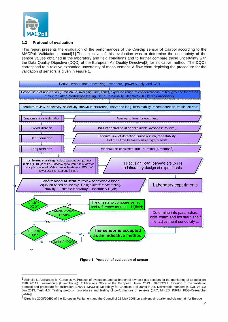
This report presents the evaluation of the performances of the Cairclip sensor of Cairpol according to the MACPoll Validation protocol[1].The objective of this evaluation was to determine the uncertainty of the sensor values obtained in the laboratory and field conditions and to further compare these uncertainty with the Data Quality Objective (DQO) of the European Air Quality Directive[2] for indicative method. The DQOs correspond to a relative expanded uncertainty of measurement. A flow chart depicting the procedure for the validation of sensors is given in Figure 1.

Figure 1: Protocol of evaluation of sensor

1 Spinelle L, Aleixandre M, Gerboles M. Protocol of evaluation and calibration of low-cost gas sensors for the monitoring of air pollution. EUR 26112. Luxembourg (Luxembourg): Publications Office of the European Union; 2013. JRC83791. Revision of the validation protocol and procedure for calibration, ENV01- MACPoll Metrology for Chemical Pollutants in Air, Deliverable number: (4.3.3), Vs 1.0, Jun 2013, Task 4.3: Testing protocol, procedures and testing of performances of sensors (JRC, MIKES, INRIM, REG-Researcher (CSIC)) 2 Directive 2008/50/EC of the European Parliament and the Council of 21 May 2008 on ambient air quality and cleaner air for Europe

10

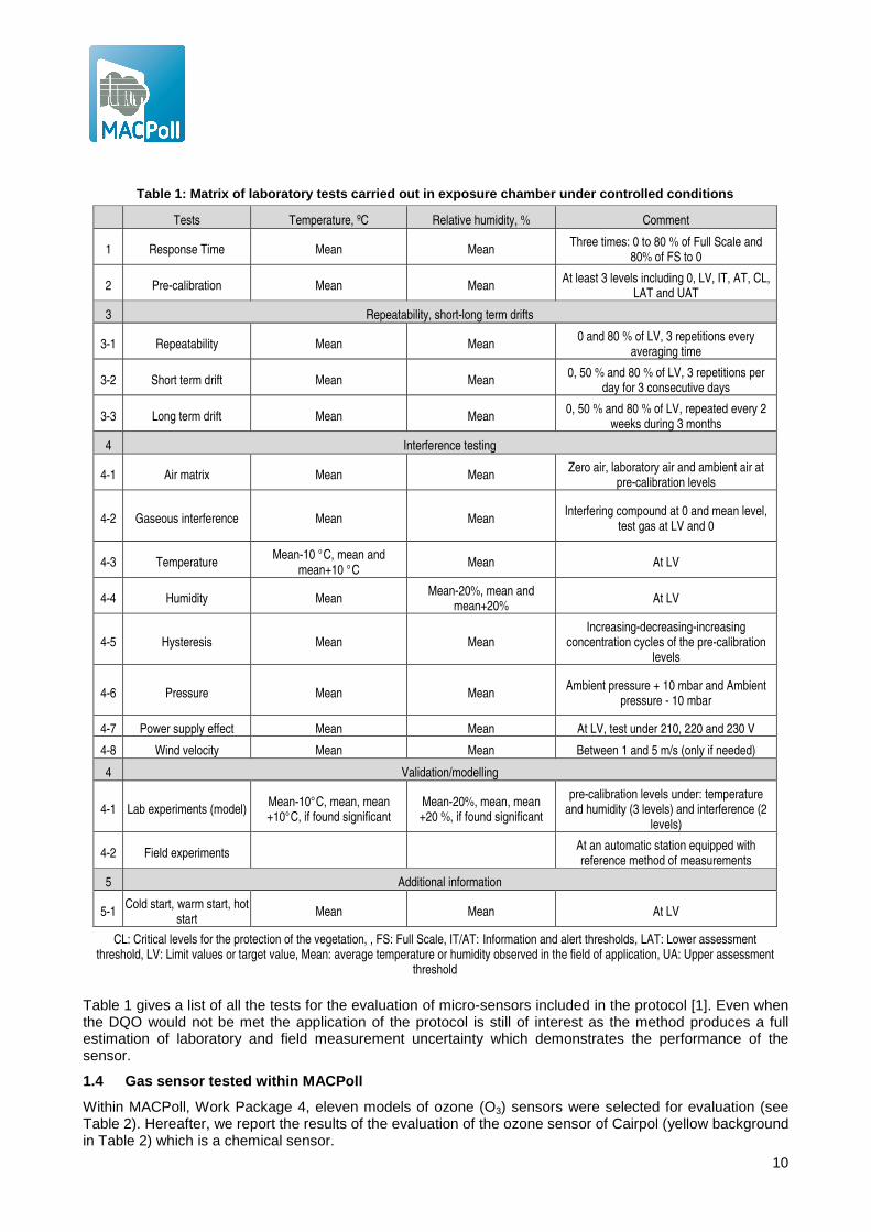
Table 1 gives a list of all the tests for the evaluation of micro-sensors included in the protocol [1]. Even when the DQO would not be met the application of the protocol is still of interest as the method produces a full estimation of laboratory and field measurement uncertainty which demonstrates the performance of the sensor.

1.4 Gas sensor tested within MACPoll

Within MACPoll, Work Package 4, eleven models of ozone (O3) sensors were selected for evaluation (see Table 2). Hereafter, we report the results of the evaluation of the ozone sensor of Cairpol (yellow background in Table 2) which is a chemical sensor.

Table 1: Matrix of laboratory tests carried out in exposure chamber under controlled conditions

Tests Temperature, ºC Relative humidity, % Comment

1 Response Time Mean Mean Three times: 0 to 80 % of Full Scale and

80% of FS to 0

2 Pre-calibration Mean Mean At least 3 levels including 0, LV, IT, AT, CL,

LAT and UAT

3 Repeatability, short-long term drifts

3-1 Repeatability Mean Mean 0 and 80 % of LV, 3 repetitions every

averaging time

3-2 Short term drift Mean Mean 0, 50 % and 80 % of LV, 3 repetitions per

day for 3 consecutive days

3-3 Long term drift Mean Mean 0, 50 % and 80 % of LV, repeated every 2

weeks during 3 months

4 Interference testing

4-1 Air matrix Mean Mean Zero air, laboratory air and ambient air at

pre-calibration levels

4-2 Gaseous interference Mean Mean Interfering compound at 0 and mean level,

test gas at LV and 0

4-3 Temperature Mean-10 °C, mean and

mean+10 °C Mean At LV

4-4 Humidity Mean Mean-20%, mean and

mean+20% At LV

4-5 Hysteresis Mean Mean Increasing-decreasing-increasing

concentration cycles of the pre-calibration levels

4-6 Pressure Mean Mean Ambient pressure + 10 mbar and Ambient

pressure - 10 mbar

4-7 Power supply effect Mean Mean At LV, test under 210, 220 and 230 V

4-8 Wind velocity Mean Mean Between 1 and 5 m/s (only if needed)

4 Validation/modelling

4-1 Lab experiments (model) Mean-10°C, mean, mean +10°C, if found significant

Mean-20%, mean, mean +20 %, if found significant

pre-calibration levels under: temperature and humidity (3 levels) and interference (2

levels)

4-2 Field experiments At an automatic station equipped with reference method of measurements

5 Additional information

5-1 Cold start, warm start, hot

start Mean Mean At LV

CL: Critical levels for the protection of the vegetation, , FS: Full Scale, IT/AT: Information and alert thresholds, LAT: Lower assessment threshold, LV: Limit values or target value, Mean: average temperature or humidity observed in the field of application, UA: Upper assessment

threshold

11

Table 2: List of O3 sensors selected for the MACPOL validation programme (this report gives the evaluat ion of the sensor with yellow background)

N° Manufacturer Model Type Data acquistion

O1 Unitec s.r.l O3 Sens 3000 Res. Analogic voltage of transmitter board

O2 Ingenieros Assessores Nano EnviSystem mote and MicroSAD datalogger, with Oz-47

sensor Res. File transfer of data loger

O3 αSense O3 sensors B4 4 Elect. Analogic Voltage of transmitter board

O4 Citytech Sensoric 4-20 mA Transmitter Board with O3E1 sensor 3 Elect. Analogic Voltage of transmitter board

O5 Citytech Sensoric 4-20 mA Transmitter Board with O3E1F sensor 3 Elect. Analogic Voltage of transmitter board

O6 Citytech A3OZ EnviroceL - 4 Elect. No testing board existing?

O7 SGX Sensortech MiCS-2610 sensor and OMC2 datalogger, Res. File transfer of data loger

O8 SGX Sensortech MiCS Oz-47 sensor and OMC3 datalogger Res. File transfer of data loger

O9 SGX Sensortech MiCS Oz-47 sensor with JRC test board Res. Development of a digital driver

O10 IMN2P Prototype WO3 sensor with MICS-EK1 Sensor Evaluation Kit Res. File transfer of the data loger

O11 FIS SP-61 sensor and evaluation test board Res. Analogic Voltage of transmitter board

O12 CairPol – F CairclipO3/NO2 3 Elect. Analogic Voltage of transmitter board

embedded in the sensor 3 Elect. and 4 Elect.: amperometric, 3 or 4 electrode sensor, Res.: resistive sensor

2 Sensor Identification

2.1 Manufacturer and supplier:

CAIRPOL, ZAC du Capra, 55, avenue Emile Antoine, 30340 Méjames les Alès – France, Tel: +33 (0)4 66 83 37 56,Fax: +33 (0)4 66 61 82 53, [email protected], www.cairpol.com

2.2 Sensor model and part number:

Sensors: Cairclip O3/NO2 ANA (analogic model), serial number (s/n) CCB0306120001 (used for the field experiments) and CCB0306120002 (used in the laboratory experiments). The sensors were not calibrated by the manufacturer.

Another Cairclip sensor, the CairClipNO2 sensor was tested for the effect of O3 on its response. This results are reported in the MACPoll report for the CairClipNO2 sensor [3].

2.3 Data processing of the sensor

No info was available about any embedded data processing system that may change the sensor responses.

2.4 Auxiliary systems such as power supply, test bo ard and data acquisition system.

A few options were included with the sensor. They consisted of: dongles USB (red for switching off the sensor, see Figure 2, and green used as a sensor base), filters, USB cable, and USB power supply.

• Power supply: a TracoPower-ESP18-05SN 5V-3.6-A power supply was used both for the laboratory tests and field tests. The power supply supplied by Cairpol was not used.

• Test board: no need for a test board, Cairclip sensors include a 5V output on their USB connector. • Data acquisition: the data acquisition board was a National Instrument, 14 bits Analog-to-digital

converter, NI-USB 6009 (National Instruments USA), NI USB 6009, USB powered. The periodicity of data acquisition was set to 100 Hz in order to eliminate electronic noise out of minute averages without further filtering needed. Within the DAQ, the sensor responses consisting in a voltage output in V were transformed into a mole ratio of O3 using the equation given in the data sheet of the sensor: O3,nmol/mol = (1000 V – 100)/10 where V is the sensor response in V.

3 Report of laboratory and in-situ validation of micro-sensor for monitoring ambient air pollution, NO9: CairClipNO2 of CAIRPOL (F), to be published

12

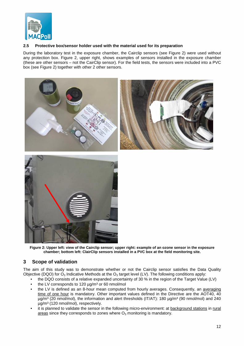
2.5 Protective box/sensor holder used with the mate rial used for its preparation

During the laboratory test in the exposure chamber, the Cairclip sensors (see Figure 2) were used without any protection box. Figure 2, upper right, shows examples of sensors installed in the exposure chamber (these are other sensors – not the CairClip sensor). For the field tests, the sensors were included into a PVC box (see Figure 2) together with other 2 other sensors.

Figure 2: Upper left: view of the Cairclip sensor; upper right: example of an ozone sensor in the expo sure chamber; bottom left: ClairClip sensors installed i n a PVC box at the field monitoring site.

3 Scope of validation

The aim of this study was to demonstrate whether or not the Cairclip sensor satisfies the Data Quality Objective (DQO) for O3 Indicative Methods at the O3 target level (LV). The following conditions apply:

• the DQO consists of a relative expanded uncertainty of 30 % in the region of the Target Value (LV) • the LV corresponds to 120 µg/m³ or 60 nmol/mol • the LV is defined as an 8-hour mean computed from hourly averages. Consequently, an averaging

time of one hour is mandatory. Other important values defined in the Directive are the AOT40, 40 µg/m³ (20 nmol/mol), the information and alert thresholds (IT/AT): 180 µg/m³ (90 nmol/mol) and 240 µg/m³ (120 nmol/mol), respectively.

• it is planned to validate the sensor in the following micro-environment: at background stations in rural areas since they corresponds to zones where O3 monitoring is mandatory.

13

Using several on-line databases and literature sources, Table 3 was established to set down the expected air composition in different micro-environments. More details are given in [4]. Using this table, the full scale of the ozone gas sensor was set to 120 nmol/mol with main mode at 60 nmol/mol. Major gas molecules in rural zones appears to be H2O, CO, NO2.

Table 3: Ambient air composition at background stat ions and rural areas between 2008 and 2010 relevant to O3 and NO2 (data from the Airbase, EUsar and TTorchs databases ). Daily data are reported unless specified.

H2O, g/m³

Further to this information it was decided to: • set the full scale to the alert threshold: about 120 nmol/mol. In table 3, the maximum O3 hourly mean

is over 150 nmol/mol while the 95th percentile is about 75 nmol/mol • to check the interference of abundant compounds: H2O, CO, NO2/NO, NH3, and SO2 to a lesser

extent. PAN was not considered because it is too difficult to generate and control. • the mean temperature and mean relative humidity were set to 22 °C and 60 %, respectively.

It is worth reminding that before using the sensor based on the validation data included in this report, it should be ascertained that the sensor is applied in the same configuration in which it was tested here. This requires using the same data acquisition and processing, the same protection box and calibration type. The sensor shall be submitted to the same regime of QA/QC as during evaluation. In addition, it is strongly recommended that sensors results are periodically compared side-by-side using the reference method.

4 Literature review:

Category under which the gas sensor falls: • the sensor behaves as a black-box without the user knowing the model equation used for the

transformation of sensor response into O3 values, • the company does not supply information about the relevant data treatment and processing that is

applied and the model equation used for the transformation of the sensor responses into O3 values • the objective of this evaluation protocol was the validation of the sensor O3 values with the possibility

to establish a correction function with the test results of the evaluation protocol if needed.

No info was found on the internet about the performance of this sensor, except a short presentation [5]

4 MACPoll, WP4, Selection of suitable micro-sensors for validation, D4.3.1 , vs 1, Mar 2012 5 https://sites.google.com/site/airsensors2013/final-materials, session Air Sensors Evaluation Project, EPA's Next Generation Air Monitoring Workshop Series, Air Sensors 2013: Data Quality & Applications, March 19 & 20, 2013, EPA's Research Triangle Park Campus, 109 T.W. Alexander Drive, Research Triangle Park, North Carolina 27711, Ron Williams, Russell Long, Melinda Beaver, (U.S. EPA), Keith Kronmiller, Sam Garvey , (Alion), Olivier Zaouak (Cairpol)

14

• model equation: since no info was available, it was assumed that the model should be linear (O3 = a + b Rs). The manufacturer gives an equation to transform the voltage output V of the sensor into a mole ratio unit: O3,nmol/mol = (1000 V – 100)/10 where V is the sensor responses in V.

• known interference, the manufacturer only mentioned Cl2. However looking at the abundance of HCl (that is thought to be more common than Cl2 in ambient air), it is unlikely that Cl2 can be present at rural sites in sufficient quantity to interfere. Thus, the effect of Cl2 on the sensor was not studied.

• Field implementation and comparison with reference method: no info available

The manufacturer gave some information about the short and long term stability and other metrological parameters (repeatability, linearity):

• Full scale: 0-250 ppb • Limit of detection: 20 ppb • Repeatability at zero: +/- 7 ppb • Repeatability à 35% of FS : +/- 20 ppb • Linearity < 10% • Short term drift for zero < 5 ppb/24hr • Short term drift of sensitivity <1% FS/24hr • Long term drift for zero < 10ppb/month • Long term drift of sensitivity < 2% FS/month • Rise time (t10-90) <90s (180 s with important HR change) • Fall time (t90-10) < 90s (180 s with important HR change) • Effect of interference : Cl about 80 % • Conditions of use : 20°C to 40°C / 15 to 90% HR wi thout condensation, 1013 mbar +/- 200 mbar • Diameter : 32 mm - Length : 62mm • Weight 55g • Maximum concentration (short time): 50ppm • Annual limit concentration (average on 1 hr) 780ppm • Recommended storage: Temperature between 5°C and 2 0°C, relative humidity 15-90 % without

condensation, pressure 1013 ±200 mbar

Personal communication of the manufacturer: a Membrapor sensor is used in the Cairclip gas sensor.

5 Laboratory experiments

5.1 Exposure chamber for test in laboratory

The gas sensors were evaluated in an exposure chamber. This chamber allows the control of O3 and other gaseous interfering compounds, temperature, relative humidity and wind velocity (see Figure 3). The exposure chamber is an “O”-shaped ring-tube system, covered with dark insulation material. The exposure chamber can accommodate the O3 micro-sensors directly inside the “O”-shaped ring-tube system.

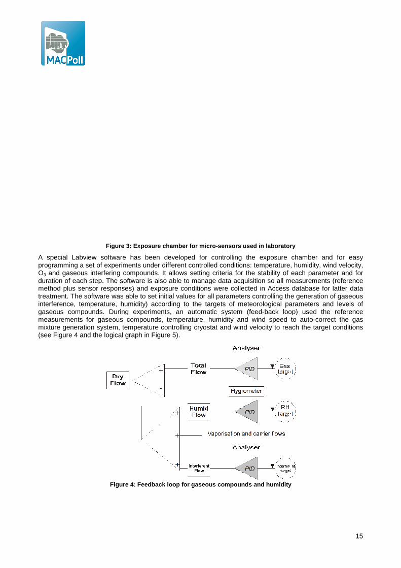
Figure 3 : Exposure chamber for micro

A special Labview software has been developed for controlling the exposure chamber and for easy programming a set of experiments under different controO3 and gaseous interfering compounds. It allows setting criteria for the stability of each parameter and for duration of each step. The software method plus sensor responses) and exposure conditions were collected in Access database for latter data treatment. The software was able to set initial values for all parameters controlling the generation of gaseous interference, temperature, humidity) according to the gaseous compounds. During experimentmeasurements for gaseous compounds, temperature, humidity and wind speed to automixture generation system, temperature controlling cryostat (see Figure 4 and the logical graph in

Figure 4 : Feedback loop

: Exposure chamber for micro -sensors used in laboratory

A special Labview software has been developed for controlling the exposure chamber and for easy programming a set of experiments under different controlled conditions: temperature, humidity, wind velocity,

and gaseous interfering compounds. It allows setting criteria for the stability of each parameter and for duration of each step. The software is also able to manage data acquisition so all measureme

) and exposure conditions were collected in Access database for latter data treatment. The software was able to set initial values for all parameters controlling the generation of gaseous

, humidity) according to the targets of meteorological parameters and levels of compounds. During experiments, an automatic system (feed-back loop)

gaseous compounds, temperature, humidity and wind speed to autotemperature controlling cryostat and wind velocity to reach

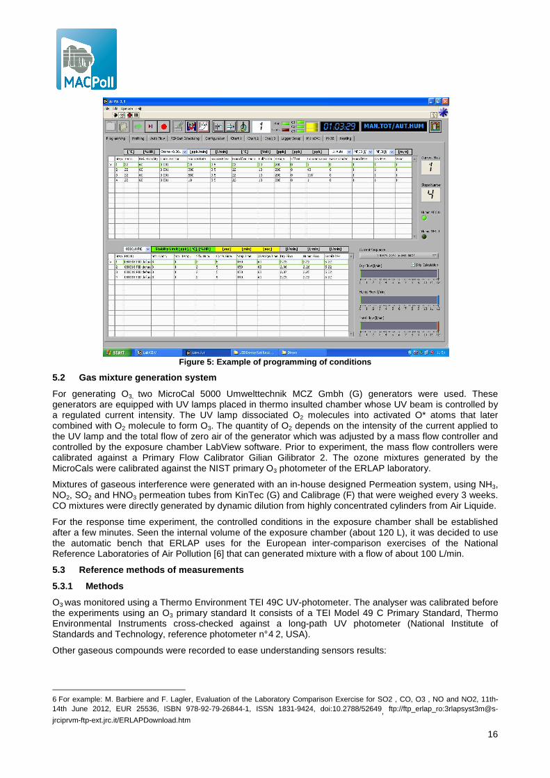
in Figure 5).

: Feedback loop for gaseous co mpounds and humidity

15

sensors used in laboratory

A special Labview software has been developed for controlling the exposure chamber and for easy lled conditions: temperature, humidity, wind velocity,

and gaseous interfering compounds. It allows setting criteria for the stability of each parameter and for also able to manage data acquisition so all measurements (reference

) and exposure conditions were collected in Access database for latter data treatment. The software was able to set initial values for all parameters controlling the generation of gaseous

meteorological parameters and levels of back loop) used the reference

gaseous compounds, temperature, humidity and wind speed to auto-correct the gas and wind velocity to reach the target conditions

mpounds and humidity

16

Figure 5: Example of programming of conditions

5.2 Gas mixture generation system

For generating O3, two MicroCal 5000 Umwelttechnik MCZ Gmbh (G) generators were used. These generators are equipped with UV lamps placed in thermo insulted chamber whose UV beam is controlled by a regulated current intensity. The UV lamp dissociated O2 molecules into activated O* atoms that later combined with O2 molecule to form O3. The quantity of O2 depends on the intensity of the current applied to the UV lamp and the total flow of zero air of the generator which was adjusted by a mass flow controller and controlled by the exposure chamber LabView software. Prior to experiment, the mass flow controllers were calibrated against a Primary Flow Calibrator Gilian Gilibrator 2. The ozone mixtures generated by the MicroCals were calibrated against the NIST primary O3 photometer of the ERLAP laboratory.

Mixtures of gaseous interference were generated with an in-house designed Permeation system, using NH3, NO2, SO2 and HNO3 permeation tubes from KinTec (G) and Calibrage (F) that were weighed every 3 weeks. CO mixtures were directly generated by dynamic dilution from highly concentrated cylinders from Air Liquide.

For the response time experiment, the controlled conditions in the exposure chamber shall be established after a few minutes. Seen the internal volume of the exposure chamber (about 120 L), it was decided to use the automatic bench that ERLAP uses for the European inter-comparison exercises of the National Reference Laboratories of Air Pollution [6] that can generated mixture with a flow of about 100 L/min.

5.3 Reference methods of measurements

5.3.1 Methods

O3 was monitored using a Thermo Environment TEI 49C UV-photometer. The analyser was calibrated before the experiments using an O3 primary standard It consists of a TEI Model 49 C Primary Standard, Thermo Environmental Instruments cross-checked against a long-path UV photometer (National Institute of Standards and Technology, reference photometer n° 4 2, USA).

Other gaseous compounds were recorded to ease understanding sensors results:

6 For example: M. Barbiere and F. Lagler, Evaluation of the Laboratory Comparison Exercise for SO2 , CO, O3 , NO and NO2, 11th-14th June 2012, EUR 25536, ISBN 978-92-79-26844-1, ISSN 1831-9424, doi:10.2788/52649, ftp://ftp_erlap_ro:3rlapsyst3m@s-

jrciprvm-ftp-ext.jrc.it/ERLAPDownload.htm

17

• NO/NOx/NO2: Thermo Environment 42 C chemiluminescence analyser, calibrated against a permeation system for NO2 and a NO working standard consisting of a gas cylinder at low concentration (down to 50 nmol/mol) certified against a Primary Reference Material of NMI VSL - NL

• SO2: Environment SA AF 21 M, calibrated with a working standard consisting of gas cylinder at low concentration (down to 50 nmol/mol) certified against a Primary Reference Material of NMI VSL - NL. The calibration of the analyser was confirmed by cross-checking with a permeation method.

• CO: Thermo Environment 48i-TLE NDIR analyser, calibrated with a CO working standard consisting of a gas cylinder at low concentration (down to 50 nmol/mol) certified against a Primary Reference Material of NMI VSL - NL.

• CO2: an infra Red sensor, Gascard NG 0-1000 µmol/mol (Edinburg Sensors – UK) was used. This sensor includes pressure correction and temperature compensation. The sensor was calibrated with a CO2 cylinder (369 ppm for Air Liquide) and zero air obtained from an ultra pure Nitrogen cylinder.

• Analyser of NH3 Ammonia Analyzer, Model 17i (courtesy of monitoring network of Bolzano/Bozen – Italy)

In addition, some other parameters were recorded and/or controlled using: • 3 Refrigerated/Heating Circulators (Model) were used to regulate the temperature of the exposure

chamber. One cryostat was used to control the temperature inside the exposure chamber, another one for the surface of the O-shaped glass tube and the last one was devoted to the control of temperature of the humid and dry air flows. These cryostats used a laboratory calibrated pt-100 probe placed inside the exposure chamber.

• 2 KZC 2/5 sensor from TERSID-It (one with ISO 17025 certificate) were used to control temperature and relative humidity. One sensor was used to monitor in real-time using our Labview software, the second one was used to register these parameter.

• 1 Testo 445 sensor (Testoterm – G) with a temperature and relative humidity probe was used as a control interface to check values inside the chamber.

• 1 Testo 452 sensor (Testoterm – G) with a temperature and relative humidity probe was used as a reference sensor and to monitor temperature and relative humidity.

• 1 wind velocity probes based on hot-wire technology was use to monitor wind velocity during tests.

• 1 pressure gauge DPI 261 from Druck (G) was used to monitor pressure inside the exposure chamber

The sampling line of each gas analyser was equipped with a Naflyon dryer to avoid interference from water vapour on O3, NOx, SO2 and CO analyser

5.3.2 Quality control

During the experiments, the O3 analyser was monthly checked using a portable O3 generator SYCOS KTO 3 (Ansyco, GmbH - G) certified against the laboratory primary standard (NIST n°42). The NO 2, SO2 and CO analyser were calibrated once a month using cylinders certified by the ERLAP laboratory. ERLAP is ISO-17025 accredited (ACCREDIA-IT, n°1362) for the meas urement of O3, NO2, SO2 and CO according to EN 14625:2012, EN 14211:2012, EN 14212:2012 and EN 14626:2012, respectively.

5.3.3 Homogeneity

Several tests were performed to confirm the homogeneity of exposure conditions in the chamber at several positions in the exposure chamber. The influence of humidity on the reference analysers was eliminated by using a naflyon dryer. The data acquisition system had a frequency of acquisition of 100 Hz and average over one minute where stored.

6 Metrological parameters

6.1 Response time

The response time of sensors, t90, was evaluated by estimating t0-90 and t90-0 (the time needed by the sensor to reach 90 % of the final stable value or 0), after a sharp change of test gas level from 0 to 80 % of the full scale (FS) (rise time) and from 80 % of FS to 0 (fall time). Four determinations of rise and fall t90 were

18

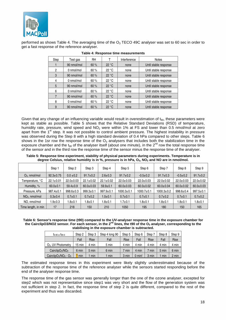
performed as shows Table 4. The averaging time of the O3 TECO 49C analyser was set to 60 sec in order to get a fast response of the reference analyser.

Table 4: Response time measurements

Step Test gas RH T Interference Notes

1 90 nmol/mol 60 % 22 °C none Until stable response









Given that any change of an influencing variable would result in overestimation of t90, these parameters were kept as stable as possible. Table 5 shows that the Relative Standard Deviations (RSD) of temperature, humidity rate, pressure, wind speed and NO2 were within 1% at FS and lower than 0.5 nmol/mol at zero apart from the 1st step. It was not possible to control ambient pressure. The highest instability in pressure was observed during the Step 8 with a high standard deviation of 0.4 hPa compared to other steps. Table 6 shows in the 1sr row the response time of the O3 analysers that includes both the stabilization time in the exposure chamber and the t90 of the analyser itself (about one minute), in the 2nd row the total response time of the sensor and in the third row the response time of the sensor minus the response time of the analyser.

Table 5: Response time experiment, stability of phy sical parameters during experiments. Temperature is in degree Celsius, relative humidity is in %, pressure is in hPa, O 3, NO2 and NO are in nmol/mol.

Step 1 Step 2 Step 3 Step 4 Step 5 Step 6 Step 7 Step 8 Step 9

O3, nmol/mol 92.3±0.75 0.0 ±0.2 91.7±0.2 2.6±0.3 91.7±0.2 -0.5±0.2 91.7±0.3 -0.5±0.2 91.7±0.2

Temperature, °C 22.1±0.01 22.0±0.03 22.1±0.02 22.1±0.02 22.0±0.03 22.0±0.03 22.0±0.02 22.0±0.03 22.0±0.02

Humidity, % 60.0±0.1 59.4±0.9 60.0±0.03 59.9±0.1 60.0±0.03 60.0±0.02 60.0±0.04 60.0±0.02 60.0±0.03

Pressure, kPa 987.4±0.1 998.6±0.3 999.3±0.1 997.9±0.1 1000.3±0.1 1000.7±0.1 1000.3±0.2 998.6±0.4 997.5±0.1

NO2, nmol/mol 0.3±0.4 0.7±0.1 0.7±0.2 1.0±0.1 0.7±0.1 0.7±0.1 0.7±0.2 0.7±0.1 0.7±0.2

NO, nmol/mol 1.9±0.3 1.8±0.1 1.8±0.1 1.8±0.1 1.7±0.1 1.8±0.1 1.8±0.1 1.8±0.1 1.8±0.1

Time length, in min 17 218 150 210 1050 195 180 150 165

Table 6: Sensor's response time (t90) compared to th e UV-analyser response time in the exposure chamber for the CairclipO3/NO2 sensor. For each sensor, in the 2nd lines, the t90 of the O 3 analyser, corresponding to the

stabilising in the exposure chamber is subtracted.

t0-90 or t90-0 Step 2 Step 3 Step 4 long 90 Step 5 Step 6 Step 7 Step 8 Step 9

Fall Rise Fall Rise Fall Rise Fall Rise

O3, UV Photometry 15 min 4 min 5 min 4 min 4 min 4 min 4 min 4 min

CairclipO3/NO2 6 min 5 min 6 min 7 min 4 min 7 min 5 min 6 min

CairclipO3/NO2 - O3 ? min 1 min 1 min 3 min 0 min! 3 min 1 min 2 min

The estimated response times in this experiment were likely slightly underestimated because of the subtraction of the response time of the reference analyser while the sensors started responding before the end of the analyser response time.

The response time of the gas sensor was generally longer than the one of the ozone analyser, excepted for step2 which was not representative since step1 was very short and the flow of the generation system was not sufficient in step 2. In fact, the response time of step 2 is quite different, compared to the rest of the experiment and thus was discarded.

19

In average, the response time of the Cairclip O3/NO2 sensor was about 1 and ½ minutes. As requested in the evaluation protocol [1], the t90 of the sensors is less than ¼ of the required averaging time of one hour and the sensors were able to reach stability within the averaging time. Compared to the majority of the tested sensors, the O3 Cairclip sensor showed a short response time.

In average, the sensor was faster in fall condition (0.7 minute) than in rise condition (2.6 minutes). Even though, this difference exceeds 10 %, it is assumed that it will not affect significantly an hourly average at rural site where ozone concentrations slowly changes.

It is stated that measuring instruments should produce individual measurements that are not influenced by previous individual measurements provided that two individual measurements are separated by at least four response times [8, 3.16]. Therefore, for the following experiments, all steps should last for at least 2.7 x 4 = 11 minutes plus the stabilisation time of the exposure chamber. However, because of other slower sensors, it was decided to have each lasting for 150 minutes, well longer that the response time of the Cairclip sensor.

Although it was not the objective of the present project, the Cairclip sensor is fast enough for mobile monitoring, being able to deliver 11 minute averages. However, micro-environment where air pollutants changes with a periodicity of a few minutes (e. g. in front of traffic light or with rapid indoor/outdoor moves) will not allow the sensor to produce independent measurements with this periodicity.

6.2 Pre calibration

The objective of this experiment was to check if the transformation of sensor responses into air pollutant concentration does not include any bias at the mean temperature and relative humidity.

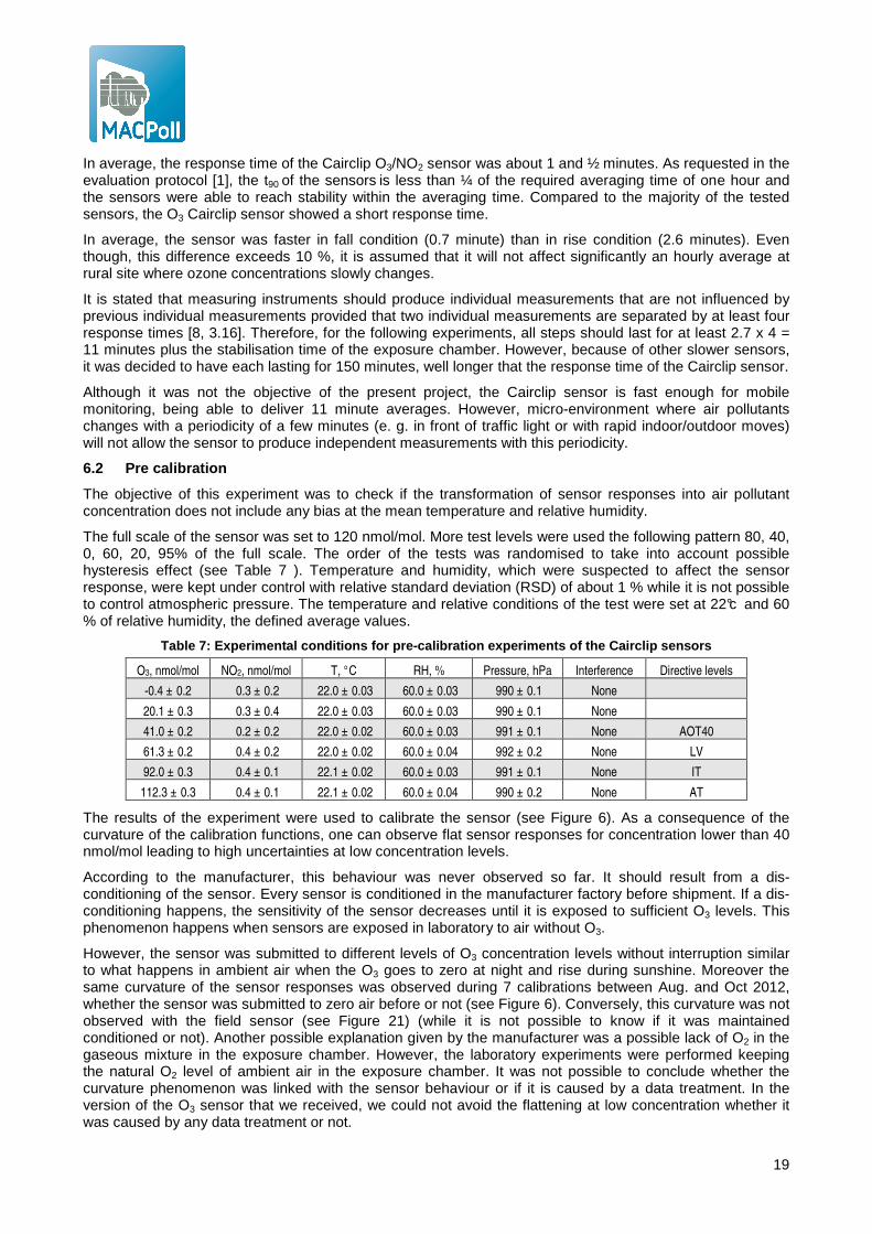
The full scale of the sensor was set to 120 nmol/mol. More test levels were used the following pattern 80, 40, 0, 60, 20, 95% of the full scale. The order of the tests was randomised to take into account possible hysteresis effect (see Table 7 ). Temperature and humidity, which were suspected to affect the sensor response, were kept under control with relative standard deviation (RSD) of about 1 % while it is not possible to control atmospheric pressure. The temperature and relative conditions of the test were set at 22°c and 60 % of relative humidity, the defined average values.

Table 7: Experimental conditions for pre-calibration experiments of the Cairclip sensors

O3, nmol/mol NO2, nmol/mol T, °C RH, % Pressure, hPa Interference Directive levels

-0.4 ± 0.2 0.3 ± 0.2 22.0 ± 0.03 60.0 ± 0.03 990 ± 0.1 None

20.1 ± 0.3 0.3 ± 0.4 22.0 ± 0.03 60.0 ± 0.03 990 ± 0.1 None

41.0 ± 0.2 0.2 ± 0.2 22.0 ± 0.02 60.0 ± 0.03 991 ± 0.1 None AOT40

61.3 ± 0.2 0.4 ± 0.2 22.0 ± 0.02 60.0 ± 0.04 992 ± 0.2 None LV

92.0 ± 0.3 0.4 ± 0.1 22.1 ± 0.02 60.0 ± 0.03 991 ± 0.1 None IT

112.3 ± 0.3 0.4 ± 0.1 22.1 ± 0.02 60.0 ± 0.04 990 ± 0.2 None AT

The results of the experiment were used to calibrate the sensor (see Figure 6). As a consequence of the curvature of the calibration functions, one can observe flat sensor responses for concentration lower than 40 nmol/mol leading to high uncertainties at low concentration levels.

According to the manufacturer, this behaviour was never observed so far. It should result from a dis-conditioning of the sensor. Every sensor is conditioned in the manufacturer factory before shipment. If a dis-conditioning happens, the sensitivity of the sensor decreases until it is exposed to sufficient O3 levels. This phenomenon happens when sensors are exposed in laboratory to air without O3.

However, the sensor was submitted to different levels of O3 concentration levels without interruption similar to what happens in ambient air when the O3 goes to zero at night and rise during sunshine. Moreover the same curvature of the sensor responses was observed during 7 calibrations between Aug. and Oct 2012, whether the sensor was submitted to zero air before or not (see Figure 6). Conversely, this curvature was not observed with the field sensor (see Figure 21) (while it is not possible to know if it was maintained conditioned or not). Another possible explanation given by the manufacturer was a possible lack of O2 in the gaseous mixture in the exposure chamber. However, the laboratory experiments were performed keeping the natural O2 level of ambient air in the exposure chamber. It was not possible to conclude whether the curvature phenomenon was linked with the sensor behaviour or if it is caused by a data treatment. In the version of the O3 sensor that we received, we could not avoid the flattening at low concentration whether it was caused by any data treatment or not.

20

The pre-calibration function was established by plotting sensor responses transformed in O3 nmol/mol with the equation given in the data sheet (see 4) versus the reference values measured by the TECO 49C analyser (see Figure 6). Each step lasted for 150 minutes once the condition of O3 concentrations, temperature and humidity were reached. The averages of the last 60 minutes are plotted. The plot at left gives only the initial calibrations and the plot at right shows all the calibration curves between August and October 2012.

The two types of calibrations function could be fitted to experimental data: either a parabolic or a sigmoid model (see Figure 6). The latter equation allowed slight improvement of the residuals of the calibration compared to the parabolic model (Eq. 1 for the initial calibration and Eq. 2 if the whole laboratory experiment).

Observing Figure 6, it appeared that in the range 40 to 80 nmol/mol, the sensor had some type of linear response with slope of 1 but an intercept of 39.9 nmol/mol. However, the residuals of the linear model are correlated with the O3 reference values. The parabolic and the sigmoid model (see Figure 6) allow removing the dependence of the residuals with the O3 reference values.

Cairclip O3/NO2, �� = log ��.��.��.�

− 1� −0.0565⁄ + 85.2for Rs > 79.1 nmol/mol Eq. 1

Cairclip O3/NO2, �� = log ��.��.��.�

− 1� −0.0499⁄ + 88.5for Rs > 76.9nmol/mol Eq. 2

Figure 6: Right: initial calibration of the Caircli p sensors at 227 calibrations between 14- Aug and 0 7-Oct

For the initial calibration with the sigmoid model, the standard uncertainty of the lack of fit of calibration, u(lof) was estimated using Eq. 3. ρmax is the maximum residual of the model and u(ref) is the uncertainty of the reference measurements set to 1.5 nmol/mol (corresponding to 5 % of relative expanded uncertainty at the LV ). If only considering O3 reference values higher than 40 nmol/mol, ρmax was equal 1.8 nmol/mol resulting in u(lof) found to be equal to 1.8 nmol/mol for the initial calibration of the sensor. Considering all calibrations between August and October 2012, the standard deviation of all residual was 2.1 nmol/mol for. u(lof), calculated using Eq. 4, was found to be equal to 2.6 nmol/mol.

�� = ��,�� ⁄ + �� Eq. 3

�� = �� + �� Eq. 4

21

In all the cases, u(lof) was small enough to be consistent with the DQO. u(lof) would not be included into the estimation of the laboratory uncertainty since the standard uncertainty of lack of fit of the experimental design/modelling (see 8) would include the standard uncertainty of the lack of fit of the calibration function.

In the tests which follows, this pre-calibration equation was applied before any other data treatment. Eq. 2, the reverse calibration function, was generally applied. However this model could only calculate O3 for responses lower than 179.0 see Eq. 2. This limit was exceeded when O3 and NO2 were at their highest values (115 and 95 nmol/mol). In this case, the parabolic model (see Figure 6 at right) was applied. Because of the curvature of the calibration function and its scattering at zero, it was difficult to apply the calibration function at low values (and sometimes at 20/40 nmol/mol). Consequently, around zero, the calibration function was not used and O3 was estimated by subtracting the average of all responses of the sensor at 0 nmol/mol to the sensor responses. The curvature of the calibration function between [0;40] nmol/mol decreased the sensor sensitivity, making it difficult to monitor around 20 nmol/mol, the AOT40, an important threshold of the Air Quality Directive at rural areas.

6.3 Repeatability, short-term and long-term drifts

The repeatability, short-term drift and long-term drift of the sensor were determined by calculating the standard deviation of sensor values for 3 consecutive averaging time periods, several consecutive days and from time to time over a longer period (originally planned every 2 weeks during three months).

The repeatability figure imposes limits on the accuracy of the calibration and allowed estimation of the limit of detection and limit of quantification of the sensor. The short term stability was used to set the maximum time between similar tests or the contribution of the short term stability to the measurement uncertainty. The long term stability was used to set the periodicity of recalibration and maximum time between similar tests. If a trend in the long term drift was identified, it would be included into the model equation or later treated as sources of uncertainty.

6.3.1 Repeatability

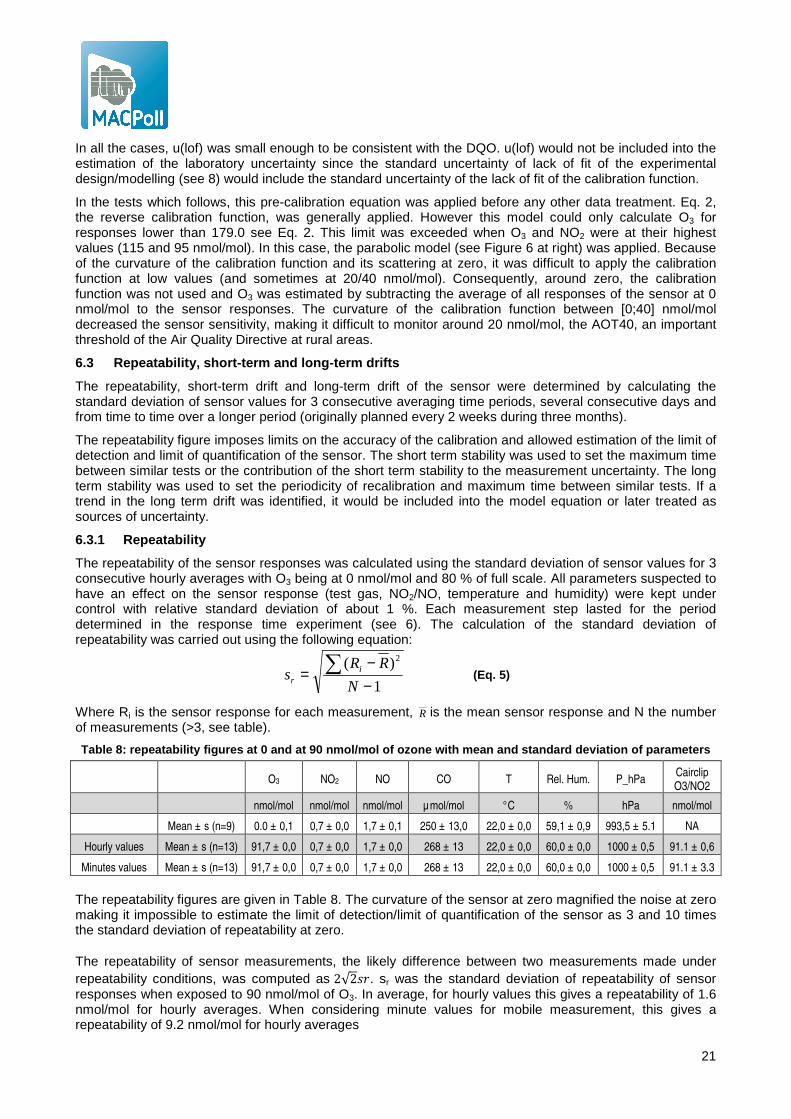
The repeatability of the sensor responses was calculated using the standard deviation of sensor values for 3 consecutive hourly averages with O3 being at 0 nmol/mol and 80 % of full scale. All parameters suspected to have an effect on the sensor response (test gas, NO2/NO, temperature and humidity) were kept under control with relative standard deviation of about 1 %. Each measurement step lasted for the period determined in the response time experiment (see 6). The calculation of the standard deviation of repeatability was carried out using the following equation:

1

)( 2

−−

= ∑N

RRs i

r (Eq. 5)

Where Ri is the sensor response for each measurement, R is the mean sensor response and N the number of measurements (>3, see table).

Table 8: repeatability figures at 0 and at 90 nmol/ mol of ozone with mean and standard deviation of pa rameters

O3 NO2 NO CO T Rel. Hum. P_hPa Cairclip O3/NO2

nmol/mol nmol/mol nmol/mol µ mol/mol °C % hPa nmol/mol

Mean ± s (n=9) 0.0 ± 0,1 0,7 ± 0,0 1,7 ± 0,1 250 ± 13,0 22,0 ± 0,0 59,1 ± 0,9 993,5 ± 5.1 NA

Hourly values Mean ± s (n=13) 91,7 ± 0,0 0,7 ± 0,0 1,7 ± 0,0 268 ± 13 22,0 ± 0,0 60,0 ± 0,0 1000 ± 0,5 91.1 ± 0,6

Minutes values Mean ± s (n=13) 91,7 ± 0,0 0,7 ± 0,0 1,7 ± 0,0 268 ± 13 22,0 ± 0,0 60,0 ± 0,0 1000 ± 0,5 91.1 ± 3.3

The repeatability figures are given in Table 8. The curvature of the sensor at zero magnified the noise at zero making it impossible to estimate the limit of detection/limit of quantification of the sensor as 3 and 10 times the standard deviation of repeatability at zero.

The repeatability of sensor measurements, the likely difference between two measurements made under repeatability conditions, was computed as 2√2��. sr was the standard deviation of repeatability of sensor responses when exposed to 90 nmol/mol of O3. In average, for hourly values this gives a repeatability of 1.6 nmol/mol for hourly averages. When considering minute values for mobile measurement, this gives a repeatability of 9.2 nmol/mol for hourly averages

22

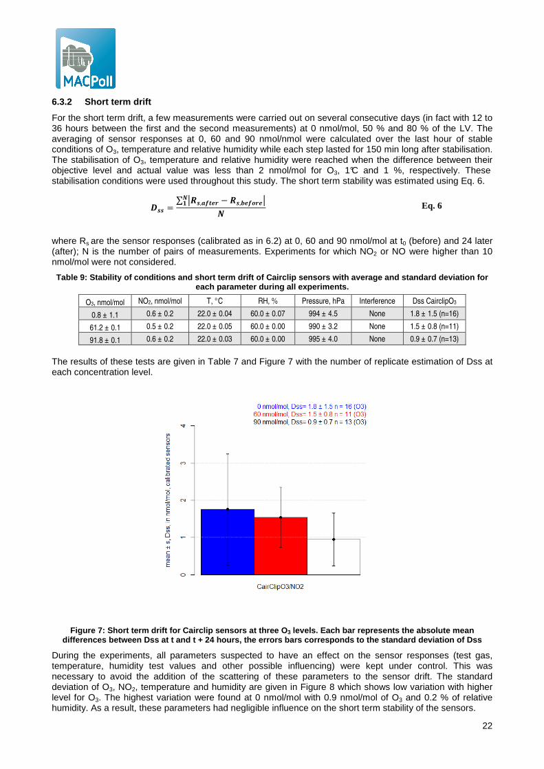
6.3.2 Short term drift

For the short term drift, a few measurements were carried out on several consecutive days (in fact with 12 to 36 hours between the first and the second measurements) at 0 nmol/mol, 50 % and 80 % of the LV. The averaging of sensor responses at 0, 60 and 90 nmol/nmol were calculated over the last hour of stable conditions of O3, temperature and relative humidity while each step lasted for 150 min long after stabilisation. The stabilisation of O3, temperature and relative humidity were reached when the difference between their objective level and actual value was less than 2 nmol/mol for O3, 1°C and 1 %, respectively. These stabilisation conditions were used throughout this study. The short term stability was estimated using Eq. 6.

�� =∑ ��,�� − ��, ��

� Eq. 6

where Rs are the sensor responses (calibrated as in 6.2) at 0, 60 and 90 nmol/mol at t0 (before) and 24 later (after); N is the number of pairs of measurements. Experiments for which NO2 or NO were higher than 10 nmol/mol were not considered.

Table 9: Stability of conditions and short term drif t of Cairclip sensors with average and standard dev iation for each parameter during all experiments.

O3, nmol/mol NO2, nmol/mol T, °C RH, % Pressure, hPa Interference Dss CairclipO3

0.8 ± 1.1 0.6 ± 0.2 22.0 ± 0.04 60.0 ± 0.07 994 ± 4.5 None 1.8 ± 1.5 (n=16)

61.2 ± 0.1 0.5 ± 0.2 22.0 ± 0.05 60.0 ± 0.00 990 ± 3.2 None 1.5 ± 0.8 (n=11)

91.8 ± 0.1 0.6 ± 0.2 22.0 ± 0.03 60.0 ± 0.00 995 ± 4.0 None 0.9 ± 0.7 (n=13)

The results of these tests are given in Table 7 and Figure 7 with the number of replicate estimation of Dss at each concentration level.

Figure 7: Short term drift for Cairclip sensors at three O 3 levels. Each bar represents the absolute mean differences between Dss at t and t + 24 hours, the errors bars corresponds to the standard deviation o f Dss

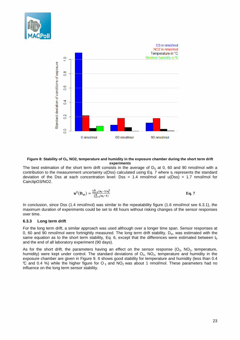
During the experiments, all parameters suspected to have an effect on the sensor responses (test gas, temperature, humidity test values and other possible influencing) were kept under control. This was necessary to avoid the addition of the scattering of these parameters to the sensor drift. The standard deviation of O3, NO2, temperature and humidity are given in Figure 8 which shows low variation with higher level for O3. The highest variation were found at 0 nmol/mol with 0.9 nmol/mol of O3 and 0.2 % of relative humidity. As a result, these parameters had negligible influence on the short term stability of the sensors.

23

Figure 8: Stability of O 3, NO2, temperature and humidity in the exposure cha mber during the short term drift experiments

The best estimation of the short term drift consists in the average of DS at 0, 60 and 90 nmol/mol with a contribution to the measurement uncertainty u(Dss) calculated using Eq. 7 where si represents the standard deviation of the Dss at each concentration level: Dss = 1.4 nmol/mol and u(Dss) = 1.7 nmol/mol for CairclipO3/NO2.

�� = ∑ ��

��

∑ ��

Eq. 7

In conclusion, since Dss (1.4 nmol/mol) was similar to the repeatability figure (1.6 nmol/mol see 6.3.1), the maximum duration of experiments could be set to 48 hours without risking changes of the sensor responses over time.

6.3.3 Long term drift

For the long term drift, a similar approach was used although over a longer time span. Sensor responses at 0, 60 and 90 nmol/mol were fortnightly measured. The long term drift stability, Dsl, was estimated with the same equation as to the short term stability, Eq. 6, except that the differences were estimated between t0 and the end of all laboratory experiment (90 days).

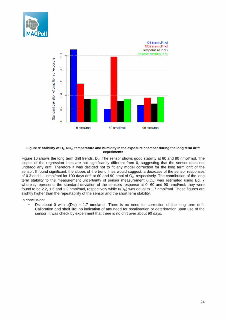
As for the short drift, the parameters having an effect on the sensor response (O3, NO2, temperature, humidity) were kept under control. The standard deviations of O3, NO2, temperature and humidity in the exposure chamber are given in Figure 9. It shows good stability for temperature and humidity (less than 0.4 °C and 0.4 %) while the higher figure for O 3 and NO2 was about 1 nmol/mol. These parameters had no influence on the long term sensor stability.

24

Figure 9: Stability of O 3, NO2, temperature and humidity in the exposure chamber during the long term drift experiments

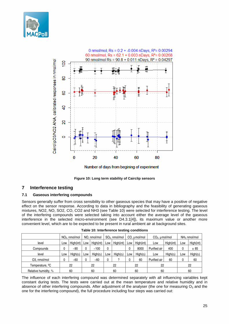
Figure 10 shows the long term drift trends, Dsl. The sensor shows good stability at 60 and 90 nmol/mol. The slopes of the regression lines are not significantly different from 0, suggesting that the sensor does not undergo any drift. Therefore it was decided not to fit any model correction for the long term drift of the sensor. If found significant, the slopes of the trend lines would suggest, a decrease of the sensor responses of 0.3 and 1.1 nmol/mol for 100 days drift at 60 and 90 nmol of O3, respectively. The contribution of the long term stability to the measurement uncertainty of sensor measurement u(Dls) was estimated using Eq. 7 where si represents the standard deviation of the sensors response at 0, 60 and 90 nmol/mol; they were found to be 2.2, 1.6 and 1.2 nmol/mol, respectively while u(Dls) was equal to 1.7 nmol/mol. These figures are slightly higher than the repeatability of the sensor and the short term stability.

In conclusion: • Dsl about 0 with u(Dsl) = 1.7 nmol/mol. There is no need for correction of the long term drift.

Calibration and shelf life: no indication of any need for recalibration or deterioration upon use of the sensor, it was check by experiment that there is no drift over about 90 days.

25

Figure 10: Long term stability of Cairclip sensors

7 Interference testing

7.1 Gaseous interfering compounds

Sensors generally suffer from cross sensibility to other gaseous species that may have a positive of negative effect on the sensor response. According to data in bibliography and the feasibility of generating gaseous mixtures, NO2, NO, SO2, CO, CO2 and NH3 (see Table 10) were selected for interference testing. The level of the interfering compounds were selected taking into account either the average level of the gaseous interference in the selected micro-environment (see D4.3.1[4]), its maximum value or another more convenient level, which are to be expected to be present in rural ambient air at background sites.

Table 10: Interference testing conditions

NO2, nmol/mol NO, nmol/mol SO2, nmol/mol CO, µ mol/mol CO2, µ mol/mol NH3, nmol/mol

level Low High(int) Low High(int) Low High(int) Low High(int) Low High(int) Low High(int)

Compounds 0 ~90 0 ~100 0 0 8000 Purified air 400 0 ± 85

level Low High(ct) Low High(ct) Low High(ct) Low High(ct) Low High(ct) Low High(ct)

O3, nmol/mol 0 ~60 0 ~60 0 ? 0 60 Purified air 60 0 60

Temperature, ºC 22 22 22 22 22 22

Relative humidity, % 60 60 60 60 60 60

The influence of each interfering compound was determined separately with all influencing variables kept constant during tests. The tests were carried out at the mean temperature and relative humidity and in absence of other interfering compounds. After adjustment of the analyser (the one for measuring O3 and the one for the interfering compound), the full procedure including four steps was carried out:

26

• The sensor response Y0: the sensor was exposed to the low level of O3 and without interfering compound;

• The sensor response Yz: the sensor was exposed to a mixture of zero gas and high level of interfering compound (at int);

• The sensor response ct: the previous scheme was repeated at a high level of O3 noted ct (generally ct equals the LV) without interfering compounds. The sensor being calibrated, its response generally was equal to ct the O3 reference level (otherwise ct represents the sensor response slightly different from the O3 reference level);

• The sensor response Yct: finally the sensor was exposed to a mixture of zero air and high level of O3 and interfering compounds at the same level as for Yz (int.).

The mixtures were supplied for a time period equal to one independent measurement, and then, three individual measurement periods (about 150 min). The level of the mixtures of the test gas and gaseous interfering compounds (apart from NH3 for which we relied on gravimetric values) were measured using reference methods of measurement with a low uncertainty of measurements (uncertainty of less than 5 %) traceable to (inter)nationally accepted standards (see 5.3).

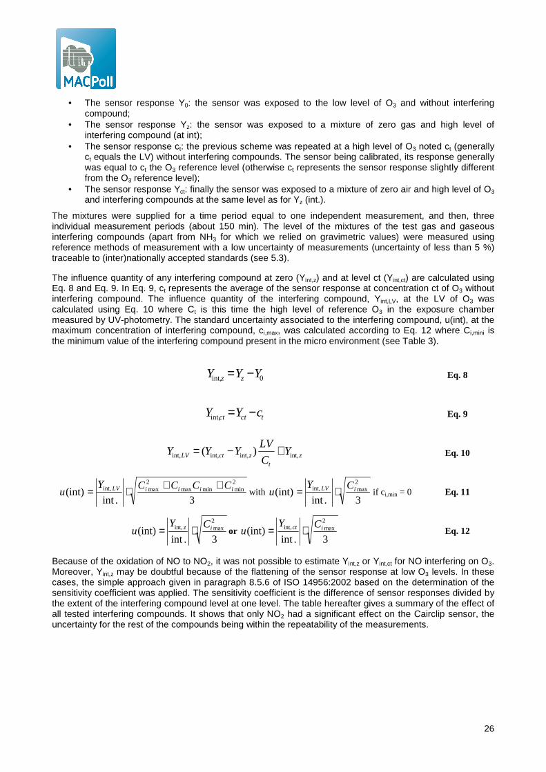
The influence quantity of any interfering compound at zero (Yint,z) and at level ct (Yint,ct) are calculated using Eq. 8 and Eq. 9. In Eq. 9, ct represents the average of the sensor response at concentration ct of O3 without interfering compound. The influence quantity of the interfering compound, Yint,LV, at the LV of O3 was calculated using Eq. 10 where Ct is this time the high level of reference O3 in the exposure chamber measured by UV-photometry. The standard uncertainty associated to the interfering compound, u(int), at the maximum concentration of interfering compound, ci,max, was calculated according to Eq. 12 where Ci,mini is the minimum value of the interfering compound present in the micro environment (see Table 3).

0int, YYY zz −= Eq. 8

tctct cYY −=int, Eq. 9

zt

zctLV YC

LVYYY int,int,int,int, )( +−= Eq. 10

3.int(int)

2minminmax

2maxint, iiiiLV CCCCY

u++⋅= with

3.int(int)

2maxint, iLV CY

u ⋅= if ci,min = 0 Eq. 11

3.int(int)

2maxint, iz CY

u ⋅= or 3.int

(int)2maxint, ict CY

u ⋅= Eq. 12

Because of the oxidation of NO to NO2, it was not possible to estimate Yint,z or Yint,ct for NO interfering on O3. Moreover, Yint,z may be doubtful because of the flattening of the sensor response at low O3 levels. In these cases, the simple approach given in paragraph 8.5.6 of ISO 14956:2002 based on the determination of the sensitivity coefficient was applied. The sensitivity coefficient is the difference of sensor responses divided by the extent of the interfering compound level at one level. The table hereafter gives a summary of the effect of all tested interfering compounds. It shows that only NO2 had a significant effect on the Cairclip sensor, the uncertainty for the rest of the compounds being within the repeatability of the measurements.

27

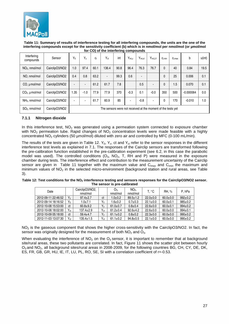
Table 11: Summary of results of interference testing for all interfering compounds, the units are the o ne of the interfering compounds except for the sensitivity co efficient (b) which is in nmol/mol per nmol/mol (or µmol/mol

for CO) of the interfering compounds

Interfering compounds

Sensor Y0 Yz ct Yct int Yint,z Yint,ct Yint,LV ci,min ci,max b u(int)

NO2, nmol/mol CairclipO3/NO2 1.0 97.4 60.1 136.4 90.8 96.4 76.3 76.7 0 40 0.84 19.5

NO, nmol/mol CairclipO3/NO2 0.4 0.8 63.2 - 99.3 0.6 - 0 25 0.006 0.1

CO, µ mol/mol CairclipO3/NO2 - - 61.2 61.7 7.8 0.5 - 0 1.5 0.070 0.1

CO2, µ mol/mol CairclipO3/NO2 1.35 -1.0 77.9 77.9 370 -0.3 0.1 -0.0 350 500 -0.000064 0.0

NH3, nmol/mol CairclipO3/NO2 - - 61.7 60.9 85 - -0.8 - 0 170 -0.010 1.0

SO2, nmol/mol CairclipO3/NO2 The sensors were not received at the moment of the tests yet

7.1.1 Nitrogen dioxide

In this interference test, NO2 was generated using a permeation system connected to exposure chamber with NO2 permeation tube. Rapid changes of NO2 concentration levels were made feasible with a highly concentrated NO2 cylinders (50 µmol/mol) diluted with zero air and controlled by MFC (0-100 mL/min).

The results of the tests are given in Table 12. Y0, Yz, ct and Yct refer to the sensor responses in the different interference test levels as explained in 7.1. The responses of the Cairclip sensors are transformed following the pre-calibration function established in the pre-calibration experiment (see 6.2, in this case the parabolic model was used). The controlled conditions (O3, NO2, T, RH and P) were measured in the exposure chamber during tests. The interference effect and contribution to the measurement uncertainty of the Cairclip sensor are given in Table 11 together with the maximum value and Cimax and Cimin the maximum and minimum values of NO2 in the selected micro-environment (background station and rural areas, see Table 3).

Table 12: Test conditions for the NO 2 interference testing and sensors responses for the CairclipO3/NO2 sensor. The sensor is pre-calibrated

Date CairclipO3/NO2,

nmol/mol

O3, nmol/mol

NO2, nmol/mol

T, °C RH, % P, hPa

2012-09-11 22:46:52 Yz 97.4±2.7 ct 1.0±0.2 89.5±1.2 22.0±0.0 60.0±0.0 992±0.2

2012-09-14 18:16:52 Y0 1.0±7.1 Y0 1.6±0.2 0.7±0.3 22.1±0.0 60.0±0.1 985±0.2

2012-10-08 15:53:00 ct 60.8±9.2 Yz 61.0±0.7 0.8±0.4 22.6±0.0 60.0±0.1 994±0.2

2012-10-08 18:02:00 Yct 137.4±2.9 Yct 61.2±0.4 92.6±4.2 22.6±0.0 60.0±0.0 994±0.1

2012-10-09 05:18:00 ct 59.4±4.7 Yz 61.1±0.2 0.8±0.2 22.3±0.0 60.0±0.0 990±0.2

2012-11-03 13:07:30 Yct 135.4±1.5 Yct 61.1±0.2 94.8±0.5 22.1±0.0 60.0±0.0 990±0.2

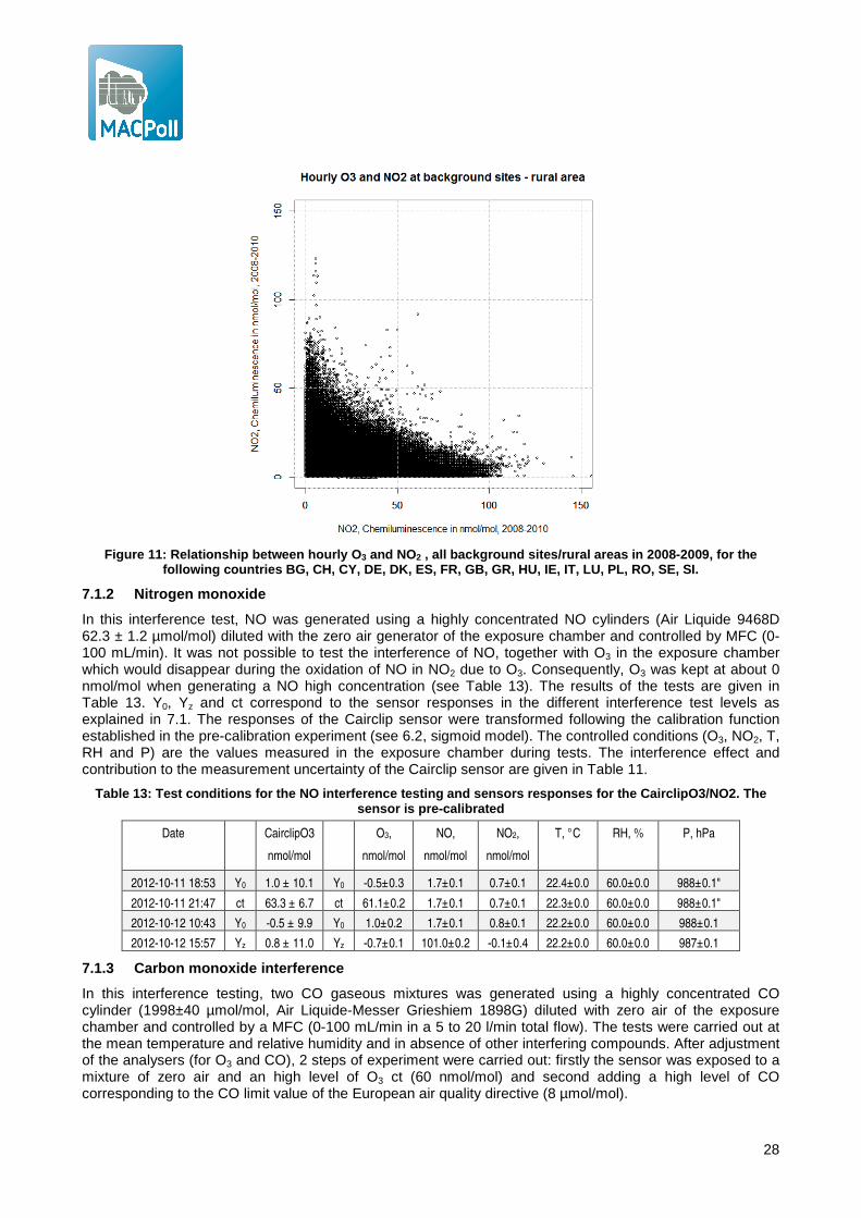
NO2 is the gaseous component that shows the higher cross-sensitivity with the CairclipO3/NO2. In fact, the sensor was originally designed for the measurement of both NO2 and O3.

When evaluating the interference of NO2 on the O3 sensor, it is important to remember that at background site/rural areas, these two pollutants are correlated. In fact, Figure 11 shows the scatter plot between hourly O3 and NO2, all background sites/rural areas in 2008-2009, for the following countries BG, CH, CY, DE, DK, ES, FR, GB, GR, HU, IE, IT, LU, PL, RO, SE, SI with a correlation coefficient of r=-0.53.

28

Figure 11: Relationship between hourly O 3 and NO2 , all background sites/rural areas in 2008-2009, f or the

following countries BG, CH, CY, DE, DK, ES, FR, GB, GR, HU, IE, IT, LU, PL, RO, SE, SI.

7.1.2 Nitrogen monoxide

In this interference test, NO was generated using a highly concentrated NO cylinders (Air Liquide 9468D 62.3 ± 1.2 µmol/mol) diluted with the zero air generator of the exposure chamber and controlled by MFC (0-100 mL/min). It was not possible to test the interference of NO, together with O3 in the exposure chamber which would disappear during the oxidation of NO in NO2 due to O3. Consequently, O3 was kept at about 0 nmol/mol when generating a NO high concentration (see Table 13). The results of the tests are given in Table 13. Y0, Yz and ct correspond to the sensor responses in the different interference test levels as explained in 7.1. The responses of the Cairclip sensor were transformed following the calibration function established in the pre-calibration experiment (see 6.2, sigmoid model). The controlled conditions (O3, NO2, T, RH and P) are the values measured in the exposure chamber during tests. The interference effect and contribution to the measurement uncertainty of the Cairclip sensor are given in Table 11.

Table 13: Test conditions for the NO interference t esting and sensors responses for the CairclipO3/NO2 . The sensor is pre-calibrated

Date CairclipO3

nmol/mol

O3,

nmol/mol

NO,

nmol/mol

NO2,

nmol/mol

T, °C RH, % P, hPa

2012-10-11 18:53 Y0 1.0 ± 10.1 Y0 -0.5±0.3 1.7±0.1 0.7±0.1 22.4±0.0 60.0±0.0 988±0.1"

2012-10-11 21:47 ct 63.3 ± 6.7 ct 61.1±0.2 1.7±0.1 0.7±0.1 22.3±0.0 60.0±0.0 988±0.1"

2012-10-12 10:43 Y0 -0.5 ± 9.9 Y0 1.0±0.2 1.7±0.1 0.8±0.1 22.2±0.0 60.0±0.0 988±0.1

2012-10-12 15:57 Yz 0.8 ± 11.0 Yz -0.7±0.1 101.0±0.2 -0.1±0.4 22.2±0.0 60.0±0.0 987±0.1

7.1.3 Carbon monoxide interference

In this interference testing, two CO gaseous mixtures was generated using a highly concentrated CO cylinder (1998±40 µmol/mol, Air Liquide-Messer Grieshiem 1898G) diluted with zero air of the exposure chamber and controlled by a MFC (0-100 mL/min in a 5 to 20 l/min total flow). The tests were carried out at the mean temperature and relative humidity and in absence of other interfering compounds. After adjustment of the analysers (for O3 and CO), 2 steps of experiment were carried out: firstly the sensor was exposed to a mixture of zero air and an high level of O3 ct (60 nmol/mol) and second adding a high level of CO corresponding to the CO limit value of the European air quality directive (8 µmol/mol).

29

The results of the test are given in Table 14 where the columns CairclipO3/NO2 give the calibrated sensor responses, O3, CO, NO2, NO, T, RH and P are the values of the conditions in the exposure during tests. The results of this experiment showed that CO had no significant influence on both the O3 sensor, as one can observe in Table 11 where the uncertainty associated with each interfering compound is given.

Table 14: Test conditions for the CO interference t esting and sensors responses for the CairclipO3/NO2 . The sensor is pre-calibrated with ozone

Date CairclipO3

nmol/mol

O3,

nmol/mol

CO,

nmol/mol

NO,

nmol/mol

NO2,

nmol/mol T, °C RH, % P, hPa

10-10-12 14:06 Yct 61.2 ± 8.8 61.1 ± 0.3 8238 ± 19.1 0.8 ± 0.2 1.7 ± 0.1 22.2 ± 0.0 60 ± 0.0 988±0.1"

11-10-12 15:45 ct 61.7 ± 7.5 61.1 ± 0.2 462.5 ± 7.5 0.7 ± 0.1 1.7 ± 0.1 22.6 ± 0.0 60 ± 0.0 988±0.1"

7.1.4 Carbon dioxide interference

The interference tests were carried out at the mean temperature and relative humidity and in the absence of any other variation from other known interfering compounds. In this interference testing, two experiments were carried out: one with air dilution of the zero air of the exposure chamber including CO2 and one using zero air filtered for CO2 from a FTIR Purge Gas Generator (85 lpm, Parker-Balston, USA remaining CO2 lower than 1 µmol/mol). The sensor responses during the two tests were then compared. Target CO2 levels in the exposure chamber were confirmed using our CO2 analyser (GasCard NH, Edinburgh Instrument) at the beginning and at the end of the experiment.

The results of the test are given in Table 15. CairclipO3 gives the calibrated sensor responses. O3, CO2, CO, NO2, NO, T, RH and P correspond to the conditions in the exposure during tests. The results of this experiment showed that CO2 had no significant influence on the O3 sensor, as one can observe in Table 11 where the uncertainty associated with each interference compound is given. The Ct level corresponds to the experiments at 60 nmol/mol of O3 of Table 11.

Table 15: Test conditions for the CO 2 interference testing and sensors responses for the CairclipO3/NO2 sensor. The sensor is pre-calibrated

Date CairclipO3 nmol/mol

O3, nmol/mol CO2,

µ mol/mol CO,

µ mol/mol NO2,

nmol/mol NO,

nmol/mol T, °C RH, % P, hPa

09-10-12 20:31 Y0 1.5 ± 10.4 1.4 ± 10.4 <1 434.3 ± 35.1 0.8 ± 0.2 1.7 ± 0.1 22.3 ± 0.0 60 ± 0.0 989 ± 0.1

09-10-12 23:20 ct 62.6 ± 4.8 62.6 ± 5.2 <1 474.0 ± 8.2 0.8 ± 0.2 1.7 ± 0.1 22.2 ± 0.0 60 ± 0.0 989 ± 0.1

10-10-12 2:22 ct 95.0 ± 5.8 93.2 ± 4.7 <1 466.5 ± 12.9 0.8 ± 0.2 1.7 ± 0.1 22.2 ± 0.0 60 ± 0.0 989 ± 0.1

11-10-12 18:53 Yz 1.1 ± 10.1 1.0 ± 10.1 ~ 370 459.6 ± 7.2 0.7 ± 0.1 1.7 ± 0.1 22.4 ± 0.0 60 ± 0.0 988 ± 0.1

11-10-12 21:47 Yct 60.2 ± 6.7 63.3 ± 63.9 ~ 370 458.7 ± 8.0 0.7 ± 0.1 1.7 ± 0.1 22.3 ± 0.0 60 ± 0.0 988 ± 0.1

12-10-12 0:27 Yct 94.4 ± 2.3 92.6 ± 9.2 ~ 370 457.0 ± 6.4 0.8 ± 0.1 1.7 ± 0.1 22.3 ± 0.0 60 ± 0.1 988 ± 0.1

7.1.5 Sulfur dioxide interference

The sensor arrived too late to be included into the SO2 interference testing experiment

7.1.6 Ammonia interference

In this interference test, NH3 was generated using a highly concentrated NH3 cylinders (Air Liquide 7162F 92.8 ± 2.8 µmol/mol) diluted with the zero air generator of the exposure chamber and controlled by MFC (0-100 mL/min). The tests were carried out at the mean temperature and relative humidity and in absence of other interfering compounds. Two steps were carried out: firstly, the sensor was exposed to a mixture of zero air and O3 (ct = 60 nmol/mol) and second adding a high level of NH3.

The results of the test are given in Table 16 where the column CairclipO3 gives the calibrated sensor responses. O3, CO, NO2, NO, T, RH and P corresponds to the conditions in the exposure chamber during tests. The results of this experiment showed that NH3 has no significant influence on the sensors as one can observe in Table 11 where the uncertainty associated with all interfering compound is given.

30

Table 16: Test conditions for the NH3 interference testing and sensors responses for the CairclipO3/NO 2 sensor. The sensors are pre-calibrated

Date CairclipO3 nmol/mol

O3, nmol/mol

NH3, nmol/mol

CO, µ mol/mol

NO, nmol/mol

NO2, nmol/mol

T, °C RH, % P, hPa

11-10-12 14:40 ct 61.7 ± 7.5 61.7 ± 0.2 0 463.7 ± 7.5 0.8 ± 0.1 1.7 ± 0.1 22.7 ± 0.0 60 ± 0.0 988 ± 0.2

11-10-12 15:45 Yct 60.9 ± 6.9 61.1 ± 0.2 85 462.5 ± 7.5 0.7 ± 0.1 1.7 ± 0.1 22.6 ± 0.0 60 ± 0.0 988 ± 0.1

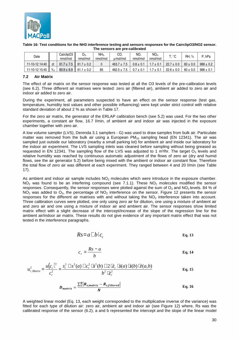
7.2 Air Matrix

The effect of air matrix on the sensor response was tested at all the O3 levels of the pre-calibration levels (see 6.2). Three different air matrixes were tested: zero air (filtered air), ambient air added to zero air and indoor air added to zero air.

During the experiment, all parameters suspected to have an effect on the sensor response (test gas, temperature, humidity test values and other possible influencing) were kept under strict control with relative standard deviation of about 2 % as shown in Table 17.

For the zero air matrix, the generator of the ERLAP calibration bench (see 5.2) was used. For the two other experiments, a constant air flow, 16.7 l/min, of ambient air and indoor air was injected in the exposure chamber together with zero air.

A low volume sampler (LVS), Derenda 3.1 samplers - G) was used to draw samples from bulk air. Particulate matter was removed from the bulk air using a European PM10 sampling head (EN 12341). The air was sampled just outside our laboratory (nearby a small parking lot) for ambient air and inside our laboratory for the indoor air experiment. The LVS sampling inlets was cleaned before sampling without being greased as requested in EN 12341. The sampling flow of the LVS was adjusted to 1 m³/hr. The target O3 levels and relative humidity was reached by continuous automatic adjustment of the flows of zero air (dry and humid flows, see the air generator 5.2) before being mixed with the ambient or indoor air constant flow. Therefore the total flow of zero air was different at each experiment. They ranged between 4 and 20 l/min (see Table 17).

As ambient and indoor air sample includes NO2 molecules which were introduce in the exposure chamber. NO2 was found to be an interfering compound (see 7.1.1). These NO2 molecules modified the sensor responses. Consequently, the sensor responses were plotted against the sum of O3 and NO2 levels. 84 % of NO2 was added to O3, the percentage of NO2 interference on the sensor. Figure 12 presents the sensor responses for the different air matrixes with and without taking the NO2 interference taken into account. Three calibration curves were plotted, one only using zero air for dilution, one using a mixture of ambient air and zero air and one using a mixture of indoor air and ambient air. The sensor responses show limited matrix effect with a slight decrease of the intercept/increase of the slope of the regression line for the ambient air/indoor air matrix. These results do not give evidence of any important matrix effect that was not tested in the interference paragraphs.

ccbaRs ⋅+=

Eq. 13

b

aRscr

−=

Eq. 14

( )22

2222

2

22,

),()()(2)()(

r

rrr

r

rMatrixr cb

barbsascbscass

c

cuu

⋅⋅⋅⋅⋅+⋅++== Eq. 15

�� =∑ ��,�� − ��,��

� Eq. 16

A weighted linear model (Eq. 13, each weight corresponded to the multiplicative inverse of the variance) was fitted for each type of dilution air: zero air, ambient air and indoor air (see Figure 12) where, Rs was the calibrated response of the sensor (6.2), a and b represented the intercept and the slope of the linear model

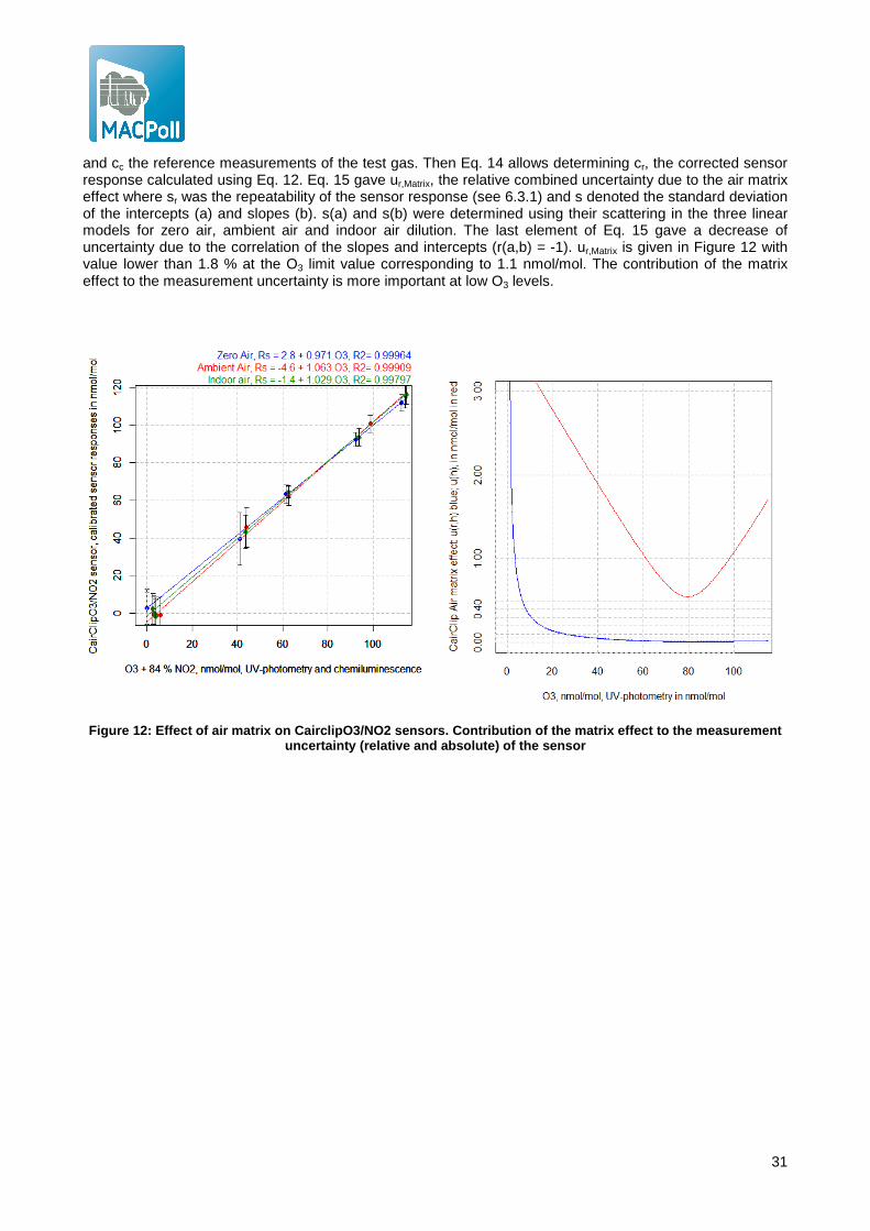
31

and cc the reference measurements of the test gas. Then Eq. 14 allows determining cr, the corrected sensor response calculated using Eq. 12. Eq. 15 gave ur,Matrix, the relative combined uncertainty due to the air matrix effect where sr was the repeatability of the sensor response (see 6.3.1) and s denoted the standard deviation of the intercepts (a) and slopes (b). s(a) and s(b) were determined using their scattering in the three linear models for zero air, ambient air and indoor air dilution. The last element of Eq. 15 gave a decrease of uncertainty due to the correlation of the slopes and intercepts (r(a,b) = -1). ur,Matrix is given in Figure 12 with value lower than 1.8 % at the O3 limit value corresponding to 1.1 nmol/mol. The contribution of the matrix effect to the measurement uncertainty is more important at low O3 levels.

Figure 12: Effect of air matrix on CairclipO3/NO2 se nsors. Contribution of the matrix effect to the mea surement uncertainty (relative and absolute) of the sensor

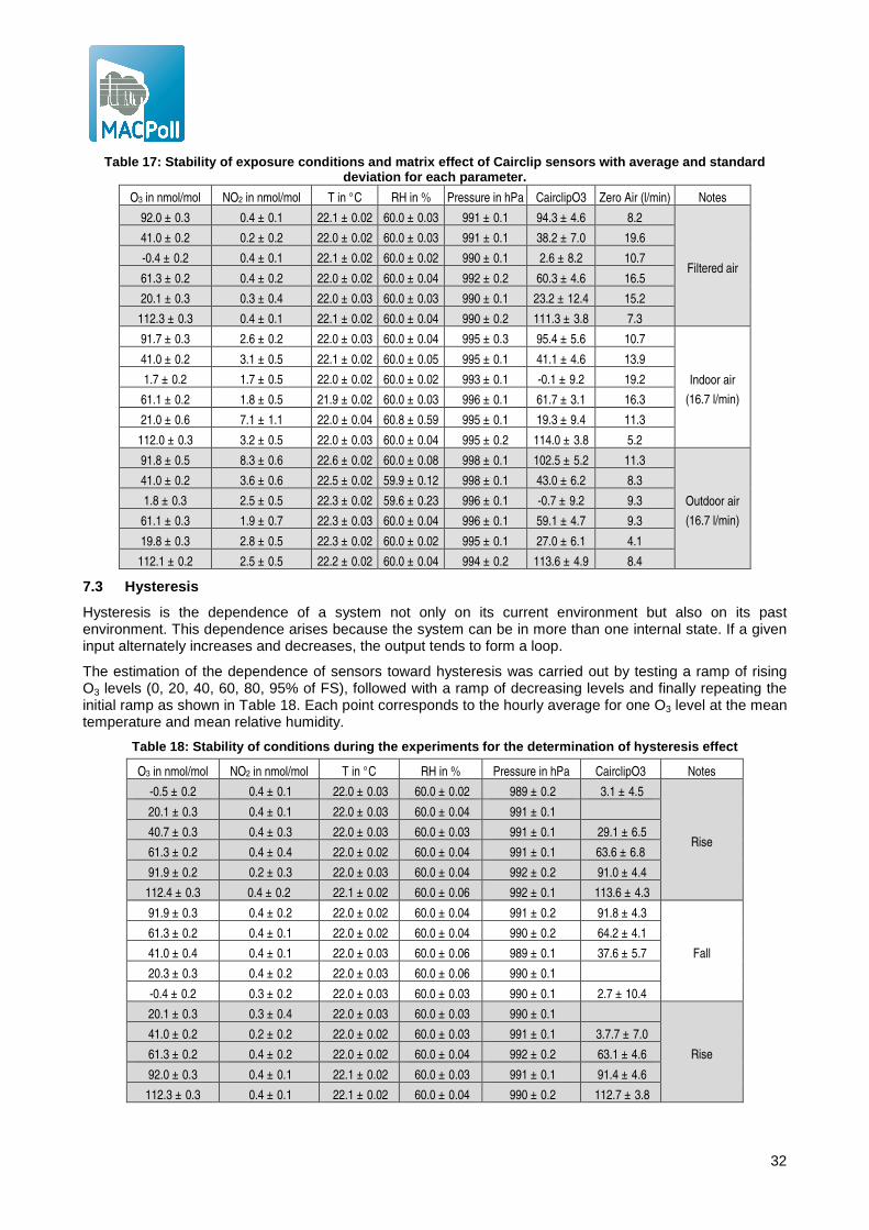
32

Table 17: Stability of exposure conditions and matri x effect of Cairclip sensors with average and stand ard deviation for each parameter.

O3 in nmol/mol NO2 in nmol/mol T in °C RH in % Pressure in hPa CairclipO3 Zero Air (l/min) Notes

92.0 ± 0.3 0.4 ± 0.1 22.1 ± 0.02 60.0 ± 0.03 991 ± 0.1 94.3 ± 4.6 8.2

Filtered air

41.0 ± 0.2 0.2 ± 0.2 22.0 ± 0.02 60.0 ± 0.03 991 ± 0.1 38.2 ± 7.0 19.6

-0.4 ± 0.2 0.4 ± 0.1 22.1 ± 0.02 60.0 ± 0.02 990 ± 0.1 2.6 ± 8.2 10.7

61.3 ± 0.2 0.4 ± 0.2 22.0 ± 0.02 60.0 ± 0.04 992 ± 0.2 60.3 ± 4.6 16.5

20.1 ± 0.3 0.3 ± 0.4 22.0 ± 0.03 60.0 ± 0.03 990 ± 0.1 23.2 ± 12.4 15.2

112.3 ± 0.3 0.4 ± 0.1 22.1 ± 0.02 60.0 ± 0.04 990 ± 0.2 111.3 ± 3.8 7.3

91.7 ± 0.3 2.6 ± 0.2 22.0 ± 0.03 60.0 ± 0.04 995 ± 0.3 95.4 ± 5.6 10.7

Indoor air

(16.7 l/min)

41.0 ± 0.2 3.1 ± 0.5 22.1 ± 0.02 60.0 ± 0.05 995 ± 0.1 41.1 ± 4.6 13.9

1.7 ± 0.2 1.7 ± 0.5 22.0 ± 0.02 60.0 ± 0.02 993 ± 0.1 -0.1 ± 9.2 19.2

61.1 ± 0.2 1.8 ± 0.5 21.9 ± 0.02 60.0 ± 0.03 996 ± 0.1 61.7 ± 3.1 16.3

21.0 ± 0.6 7.1 ± 1.1 22.0 ± 0.04 60.8 ± 0.59 995 ± 0.1 19.3 ± 9.4 11.3

112.0 ± 0.3 3.2 ± 0.5 22.0 ± 0.03 60.0 ± 0.04 995 ± 0.2 114.0 ± 3.8 5.2

91.8 ± 0.5 8.3 ± 0.6 22.6 ± 0.02 60.0 ± 0.08 998 ± 0.1 102.5 ± 5.2 11.3

Outdoor air

(16.7 l/min)

41.0 ± 0.2 3.6 ± 0.6 22.5 ± 0.02 59.9 ± 0.12 998 ± 0.1 43.0 ± 6.2 8.3

1.8 ± 0.3 2.5 ± 0.5 22.3 ± 0.02 59.6 ± 0.23 996 ± 0.1 -0.7 ± 9.2 9.3

61.1 ± 0.3 1.9 ± 0.7 22.3 ± 0.03 60.0 ± 0.04 996 ± 0.1 59.1 ± 4.7 9.3

19.8 ± 0.3 2.8 ± 0.5 22.3 ± 0.02 60.0 ± 0.02 995 ± 0.1 27.0 ± 6.1 4.1

112.1 ± 0.2 2.5 ± 0.5 22.2 ± 0.02 60.0 ± 0.04 994 ± 0.2 113.6 ± 4.9 8.4

7.3 Hysteresis

Hysteresis is the dependence of a system not only on its current environment but also on its past environment. This dependence arises because the system can be in more than one internal state. If a given input alternately increases and decreases, the output tends to form a loop.

The estimation of the dependence of sensors toward hysteresis was carried out by testing a ramp of rising O3 levels (0, 20, 40, 60, 80, 95% of FS), followed with a ramp of decreasing levels and finally repeating the initial ramp as shown in Table 18. Each point corresponds to the hourly average for one O3 level at the mean temperature and mean relative humidity.

Table 18: Stability of conditions during the experim ents for the determination of hysteresis effect

O3 in nmol/mol NO2 in nmol/mol T in °C RH in % Pressure in hPa CairclipO3 Notes

-0.5 ± 0.2 0.4 ± 0.1 22.0 ± 0.03 60.0 ± 0.02 989 ± 0.2 3.1 ± 4.5

Rise

20.1 ± 0.3 0.4 ± 0.1 22.0 ± 0.03 60.0 ± 0.04 991 ± 0.1

40.7 ± 0.3 0.4 ± 0.3 22.0 ± 0.03 60.0 ± 0.03 991 ± 0.1 29.1 ± 6.5

61.3 ± 0.2 0.4 ± 0.4 22.0 ± 0.02 60.0 ± 0.04 991 ± 0.1 63.6 ± 6.8

91.9 ± 0.2 0.2 ± 0.3 22.0 ± 0.03 60.0 ± 0.04 992 ± 0.2 91.0 ± 4.4

112.4 ± 0.3 0.4 ± 0.2 22.1 ± 0.02 60.0 ± 0.06 992 ± 0.1 113.6 ± 4.3

91.9 ± 0.3 0.4 ± 0.2 22.0 ± 0.02 60.0 ± 0.04 991 ± 0.2 91.8 ± 4.3

Fall

61.3 ± 0.2 0.4 ± 0.1 22.0 ± 0.02 60.0 ± 0.04 990 ± 0.2 64.2 ± 4.1

41.0 ± 0.4 0.4 ± 0.1 22.0 ± 0.03 60.0 ± 0.06 989 ± 0.1 37.6 ± 5.7

20.3 ± 0.3 0.4 ± 0.2 22.0 ± 0.03 60.0 ± 0.06 990 ± 0.1

-0.4 ± 0.2 0.3 ± 0.2 22.0 ± 0.03 60.0 ± 0.03 990 ± 0.1 2.7 ± 10.4

20.1 ± 0.3 0.3 ± 0.4 22.0 ± 0.03 60.0 ± 0.03 990 ± 0.1

Rise

41.0 ± 0.2 0.2 ± 0.2 22.0 ± 0.02 60.0 ± 0.03 991 ± 0.1 3.7.7 ± 7.0

61.3 ± 0.2 0.4 ± 0.2 22.0 ± 0.02 60.0 ± 0.04 992 ± 0.2 63.1 ± 4.6

92.0 ± 0.3 0.4 ± 0.1 22.1 ± 0.02 60.0 ± 0.03 991 ± 0.1 91.4 ± 4.6

112.3 ± 0.3 0.4 ± 0.1 22.1 ± 0.02 60.0 ± 0.04 990 ± 0.2 112.7 ± 3.8

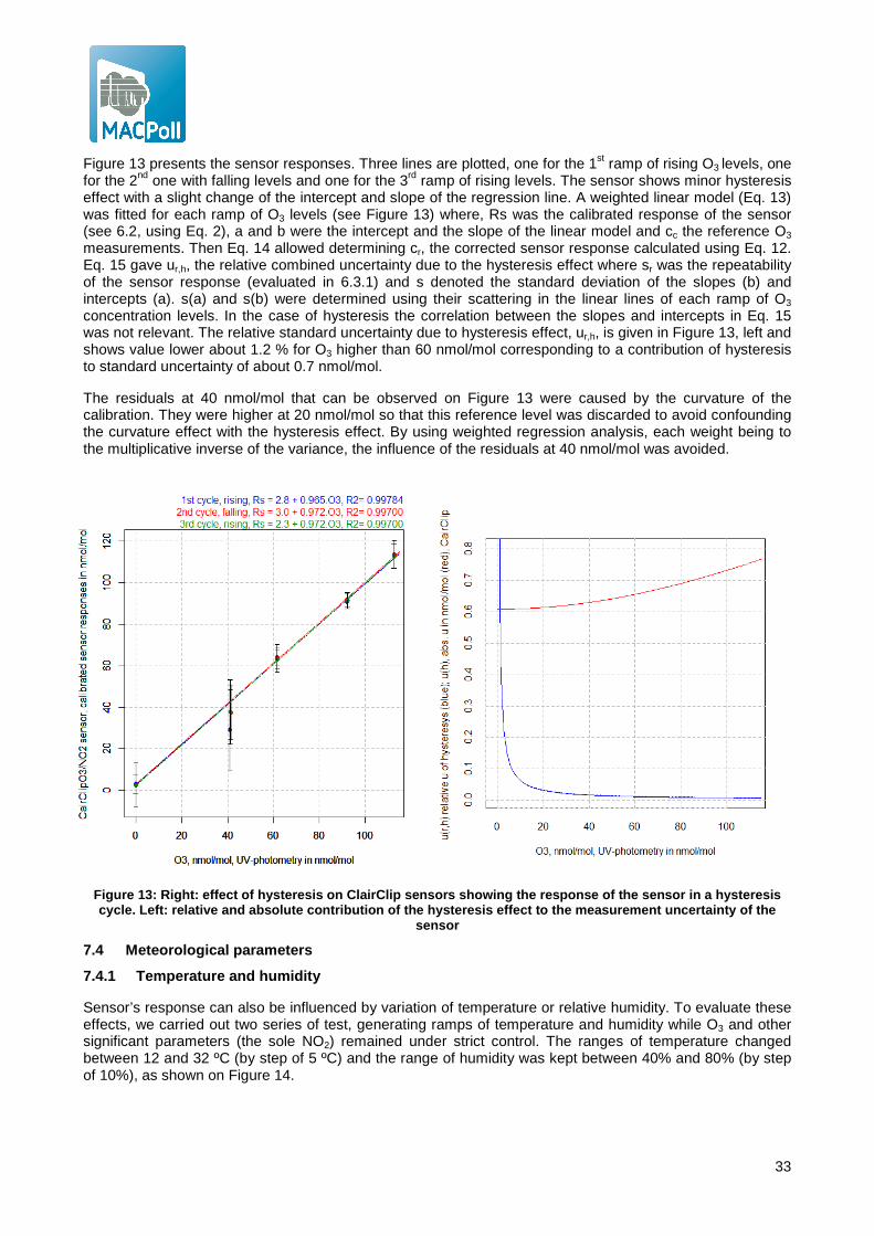
33

Figure 13 presents the sensor responses. Three lines are plotted, one for the 1st ramp of rising O3 levels, one for the 2nd one with falling levels and one for the 3rd ramp of rising levels. The sensor shows minor hysteresis effect with a slight change of the intercept and slope of the regression line. A weighted linear model (Eq. 13) was fitted for each ramp of O3 levels (see Figure 13) where, Rs was the calibrated response of the sensor (see 6.2, using Eq. 2), a and b were the intercept and the slope of the linear model and cc the reference O3 measurements. Then Eq. 14 allowed determining cr, the corrected sensor response calculated using Eq. 12. Eq. 15 gave ur,h, the relative combined uncertainty due to the hysteresis effect where sr was the repeatability of the sensor response (evaluated in 6.3.1) and s denoted the standard deviation of the slopes (b) and intercepts (a). s(a) and s(b) were determined using their scattering in the linear lines of each ramp of O3 concentration levels. In the case of hysteresis the correlation between the slopes and intercepts in Eq. 15 was not relevant. The relative standard uncertainty due to hysteresis effect, ur,h, is given in Figure 13, left and shows value lower about 1.2 % for O3 higher than 60 nmol/mol corresponding to a contribution of hysteresis to standard uncertainty of about 0.7 nmol/mol.

The residuals at 40 nmol/mol that can be observed on Figure 13 were caused by the curvature of the calibration. They were higher at 20 nmol/mol so that this reference level was discarded to avoid confounding the curvature effect with the hysteresis effect. By using weighted regression analysis, each weight being to the multiplicative inverse of the variance, the influence of the residuals at 40 nmol/mol was avoided.

Figure 13: Right: effect of hysteresis on ClairClip sensors showing the response of the sensor in a hy steresis cycle. Left: relative and absolute contribution of the hysteresis effect to the measurement uncertaint y of the

sensor

7.4 Meteorological parameters

7.4.1 Temperature and humidity

Sensor’s response can also be influenced by variation of temperature or relative humidity. To evaluate these effects, we carried out two series of test, generating ramps of temperature and humidity while O3 and other significant parameters (the sole NO2) remained under strict control. The ranges of temperature changed between 12 and 32 ºC (by step of 5 ºC) and the range of humidity was kept between 40% and 80% (by step of 10%), as shown on Figure 14.

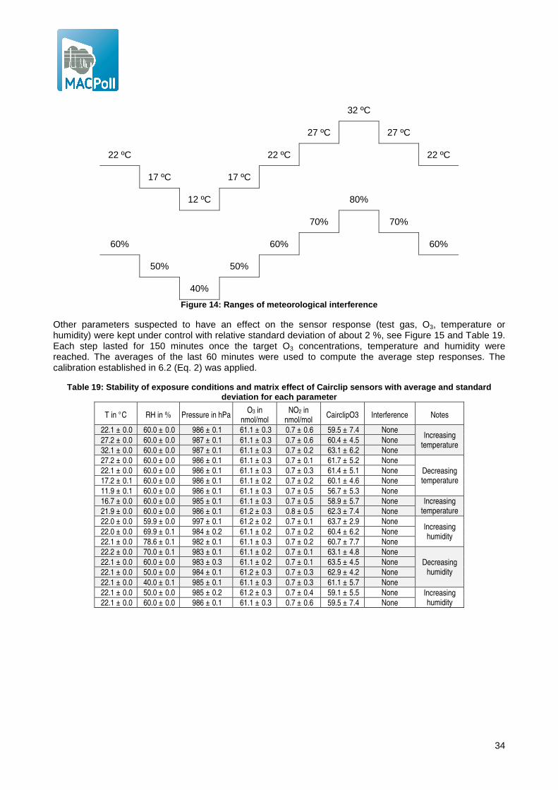
34

32 ºC

27 ºC 27 ºC

22 ºC 22 ºC 22 ºC

17 ºC 17 ºC

12 ºC 80%

70% 70%

60% 60% 60%

50% 50%

40%

Figure 14: Ranges of meteorological interference

Other parameters suspected to have an effect on the sensor response (test gas, O3, temperature or humidity) were kept under control with relative standard deviation of about 2 %, see Figure 15 and Table 19. Each step lasted for 150 minutes once the target O3 concentrations, temperature and humidity were reached. The averages of the last 60 minutes were used to compute the average step responses. The calibration established in 6.2 (Eq. 2) was applied.

Table 19: Stability of exposure conditions and matri x effect of Cairclip sensors with average and stand ard deviation for each parameter

T in °C RH in % Pressure in hPa O3 in

nmol/mol NO2 in

nmol/mol CairclipO3 Interference Notes

22.1 ± 0.0 60.0 ± 0.0 986 ± 0.1 61.1 ± 0.3 0.7 ± 0.6 59.5 ± 7.4 None Increasing

temperature 27.2 ± 0.0 60.0 ± 0.0 987 ± 0.1 61.1 ± 0.3 0.7 ± 0.6 60.4 ± 4.5 None

32.1 ± 0.0 60.0 ± 0.0 987 ± 0.1 61.1 ± 0.3 0.7 ± 0.2 63.1 ± 6.2 None

27.2 ± 0.0 60.0 ± 0.0 986 ± 0.1 61.1 ± 0.3 0.7 ± 0.1 61.7 ± 5.2 None

Decreasing temperature

22.1 ± 0.0 60.0 ± 0.0 986 ± 0.1 61.1 ± 0.3 0.7 ± 0.3 61.4 ± 5.1 None

17.2 ± 0.1 60.0 ± 0.0 986 ± 0.1 61.1 ± 0.2 0.7 ± 0.2 60.1 ± 4.6 None

11.9 ± 0.1 60.0 ± 0.0 986 ± 0.1 61.1 ± 0.3 0.7 ± 0.5 56.7 ± 5.3 None

16.7 ± 0.0 60.0 ± 0.0 985 ± 0.1 61.1 ± 0.3 0.7 ± 0.5 58.9 ± 5.7 None Increasing temperature 21.9 ± 0.0 60.0 ± 0.0 986 ± 0.1 61.2 ± 0.3 0.8 ± 0.5 62.3 ± 7.4 None

22.0 ± 0.0 59.9 ± 0.0 997 ± 0.1 61.2 ± 0.2 0.7 ± 0.1 63.7 ± 2.9 None Increasing humidity

22.0 ± 0.0 69.9 ± 0.1 984 ± 0.2 61.1 ± 0.2 0.7 ± 0.2 60.4 ± 6.2 None

22.1 ± 0.0 78.6 ± 0.1 982 ± 0.1 61.1 ± 0.3 0.7 ± 0.2 60.7 ± 7.7 None

22.2 ± 0.0 70.0 ± 0.1 983 ± 0.1 61.1 ± 0.2 0.7 ± 0.1 63.1 ± 4.8 None

Decreasing humidity

22.1 ± 0.0 60.0 ± 0.0 983 ± 0.3 61.1 ± 0.2 0.7 ± 0.1 63.5 ± 4.5 None

22.1 ± 0.0 50.0 ± 0.0 984 ± 0.1 61.2 ± 0.3 0.7 ± 0.3 62.9 ± 4.2 None

22.1 ± 0.0 40.0 ± 0.1 985 ± 0.1 61.1 ± 0.3 0.7 ± 0.3 61.1 ± 5.7 None

22.1 ± 0.0 50.0 ± 0.0 985 ± 0.2 61.2 ± 0.3 0.7 ± 0.4 59.1 ± 5.5 None Increasing humidity 22.1 ± 0.0 60.0 ± 0.0 986 ± 0.1 61.1 ± 0.3 0.7 ± 0.6 59.5 ± 7.4 None

35

Figure 15: Sensitivity of CairClipO3/NO 2 sensor toward relative humidity (left) and tempera ture (right. The error bars give the standard deviations of the sensor res ponses during the last hour of each test levels

The influences of temperature and humidity on the sensor responses are shown in Figure 15. In average, the sensor did not show any sensitivity to relative humidity (the slope of the regression line being insignificantly different from 0 (actual value: 0.0077 ± 0.055). Regarding temperature, the sensor showed a slight significant dependence with a slope equal to 0.24 ± 0.04. The sensor’s response increased with temperature. Moreover, a slight hysteresis effect was observed (see Figure 15 and detailed values in Table 15) for the humidity effect. In fact, the sensor responses showed a delay from test level to test level. For example, the sensor responses kept on increasing one step after the maximum temperature/humidity and conversely. The variation of the sensor response against temperature and relative humidity was estimated with Eq. 17 using the sensitivity coefficient b, the slope of the regression lines, to estimate the standard uncertainty,�� . A

36

contribution of the hysteresis of temperature and humidity was added. These contributions were set to the maximum deviation or the regression lines.

u(�) = ��

�+��,��

��/�

Eq. 17

Where x is the tested parameter, b is the slope of the regression line of the sensor responses versus temperature and humidity, � !� and � "# the maximum and minimum values encountered in real ambient for parameter � and ρmax is the maximum residuals between the regression line and the sensor responses or the one at the LV.

Assuming a temperature range between 15 and 45 °C, the maximum residual of the linear fit being 3.3 nmol/mol, the contribution of the temperature effect was u(T) = 1.9 nmol/mol with correction of the sensor for the temperature effect or u(T) = 4.6 nmol/mol without correction of the sensor for the relative humidity effect.

Assuming a relative humidity range between 30 and 95 %, the maximum residual of the linear fit being 2.3 nmol/mol, the contribution of the relative humidity effect was u(RH) = 1.4 nmol/mol. The slope of the regression line was not significant and it was not taken into account.

7.4.2 Wind velocity effect

A test for wind speed ranging between 0.8 and 5 m/s of wind velocity was performed. However, the Cairclip sensor or its data acquisition system did not work correctly during the experiment (sensor responses were negative likely because the internal battery was not powered during this test). An indirect evaluation of the effect of wind velocity was performed by plotting the responses of the long drift experiment at 60 and 90 nmol/mol versus the wind velocity during these tests that show some variation (see Figure 16). The slope of trend line could be used as the sensitivity coefficient of the sensor responses to wind velocity. The observed figures appeared overestimated (-3.8 and -1.6 nmol/mol per m/s of wind velocity at 90 and 60 nmol/mol, respectively). In fact, this experiment includes a few shortcomings: extrapolation due to the limited range of wind velocities with differences between sensor responses being only slightly higher than the repeatability of results. Moreover, a few covariates were not independent (these tests were drawn from the results of other experiments: drift estimation, power supply ...). A range of variation of wind velocity of 0 to 5 ms would lead to a standard uncertainty of 7.5 nmol/mol. This high value was rather unlikely. In fact, we assumed that the changes observed in this experiment were coming from dependent covariates instead of wind velocity.

When reporting these results, the manufacturer informed that the wind effect strongly depends on the direction of the wind and the precise positioning of the sensor whose microfan can be disturbed. Cairpol recommends using their sensor protective box called Cairbox.

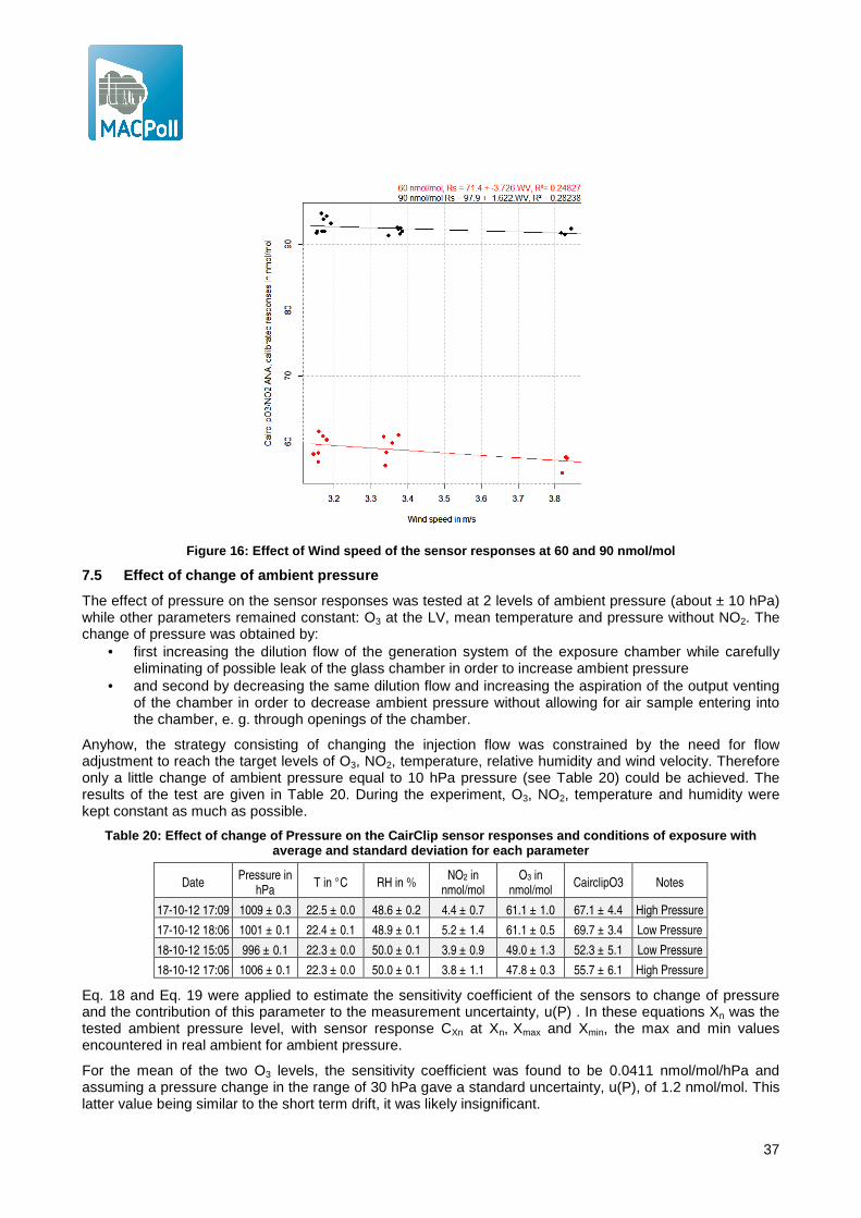
37

Figure 16: Effect of Wind speed of the sensor respon ses at 60 and 90 nmol/mol

7.5 Effect of change of ambient pressure

The effect of pressure on the sensor responses was tested at 2 levels of ambient pressure (about ± 10 hPa) while other parameters remained constant: O3 at the LV, mean temperature and pressure without NO2. The change of pressure was obtained by:

• first increasing the dilution flow of the generation system of the exposure chamber while carefully eliminating of possible leak of the glass chamber in order to increase ambient pressure

• and second by decreasing the same dilution flow and increasing the aspiration of the output venting of the chamber in order to decrease ambient pressure without allowing for air sample entering into the chamber, e. g. through openings of the chamber.

Anyhow, the strategy consisting of changing the injection flow was constrained by the need for flow adjustment to reach the target levels of O3, NO2, temperature, relative humidity and wind velocity. Therefore only a little change of ambient pressure equal to 10 hPa pressure (see Table 20) could be achieved. The results of the test are given in Table 20. During the experiment, O3, NO2, temperature and humidity were kept constant as much as possible.

Table 20: Effect of change of Pressure on the CairCli p sensor responses and conditions of exposure with average and standard deviation for each parameter

Date Pressure in

hPa T in °C RH in %

NO2 in nmol/mol

O3 in nmol/mol

CairclipO3 Notes

17-10-12 17:09 1009 ± 0.3 22.5 ± 0.0 48.6 ± 0.2 4.4 ± 0.7 61.1 ± 1.0 67.1 ± 4.4 High Pressure

17-10-12 18:06 1001 ± 0.1 22.4 ± 0.1 48.9 ± 0.1 5.2 ± 1.4 61.1 ± 0.5 69.7 ± 3.4 Low Pressure

18-10-12 15:05 996 ± 0.1 22.3 ± 0.0 50.0 ± 0.1 3.9 ± 0.9 49.0 ± 1.3 52.3 ± 5.1 Low Pressure

18-10-12 17:06 1006 ± 0.1 22.3 ± 0.0 50.0 ± 0.1 3.8 ± 1.1 47.8 ± 0.3 55.7 ± 6.1 High Pressure

Eq. 18 and Eq. 19 were applied to estimate the sensitivity coefficient of the sensors to change of pressure and the contribution of this parameter to the measurement uncertainty, u(P) . In these equations Xn was the tested ambient pressure level, with sensor response CXn at Xn, Xmax and Xmin, the max and min values encountered in real ambient for ambient pressure.

For the mean of the two O3 levels, the sensitivity coefficient was found to be 0.0411 nmol/mol/hPa and assuming a pressure change in the range of 30 hPa gave a standard uncertainty, u(P), of 1.2 nmol/mol. This latter value being similar to the short term drift, it was likely insignificant.

38

7.6 Effect of change in power supply

The effect of power supply on the sensor responses was tested at 3 levels of voltage (210, 220 and 230 V) while other parameters remaining constant: O3 at the LV, and mean temperature and pressure without NO2. O3, NO2, temperature and humidity were kept as constant as possible during the experiment. In this experiment, the power supply of the sensor was changed using a variable rheostat, model Rheothor ADB RT 10 27/B. The results of the test are given in Table 20.

Table 21: Effect of change of power supply on the Ca irclip sensor responses and conditions of exposure with average and standard deviation for each parameter

Date Voltage T in °C RH in % Pressure in

hPa O3 in

nmol/mol NO2 in

nmol/mol CairclipO3

06-11-12 16:00 220 V 22.3 ± 0.1 60.0 ± 0.1 991 ± 0.3 61.1 ± 0.2 4.9 ± 0.3 63.7 ± 7.4

06-11-12 17:00 230 V 22.2 ± 0.0 60.0 ± 0.1 992 ± 0.2 61.1 ± 0.2 5.0 ± 0.3 64.6 ± 6.9

06-11-12 17:31 210 V 22.2 ± 0.1 60.0 ± 0.1 992 ± 0.2 61.1 ± 0.2 4.9 ± 0.2 55.9 ± 8.2

07-11-12 11:20 210 V 22.1 ± 0.1 60.0 ± 0.1 1003 ± 0.1 61.1 ± 0.2 5.0 ± 0.3 58.3 ± 9.4

07-11-12 13:18 230 V 22.1 ± 0.1 60.0 ± 0.1 1002 ± 0.1 61.2 ± 0.3 5.0 ± 0.4 63.7 ± 7.9

07-11-12 17:20 220 V 22.1 ± 0.1 60.0 ± 0.1 1003 ± 0.3 61.1 ± 0.2 4.7 ± 5.5 64.2 ± 8.4

Eq. 18 and Eq. 19 were applied to estimate the sensitivity coefficient of the sensors to changes of power supply and the contribution of this parameter to the measurement uncertainty of the sensor, u(Xp). In these equations Xn is the tested ambient voltage level, with sensor response CXn at Xn, Xmax and Xmin the max and min values expected voltage in field operation.

12

12

XX

CC

X

C XX

−−

=∆∆

Eq. 18

3)( minmax

12

12XX

XX

CCXu XX

p

−⋅−−

= Eq. 19

In average the sensitivity coefficient was found to be 0.39 nmol/mol/V and assuming a voltage change of 20 Volts resulted in a standard uncertainty of u(V) equal to 4.4 nmol/mol. One may observe that the effect occurred mainly at 210 V while between 220 and 230 V the sensor responses remained rather constant within 1 nmol/mol change that is consistent with the repeatability figure. In fact, applying a t test (unequal sample sizes 120 and 240 and unequal variances 8.8 and 7.7) between the average sensor response at 210 V and 220-230 V gave a t value of 3.06 showing that the difference is significant between these two groups of voltages.

7.7 Choice of tested interfering parameters in full factorial design

Even though the sensor was designed to measure both NO2 and O3, when the measurement of the sole O3 is intended NO2 acts as an interfering compound. The major cross sensitivities showed by the CairClipO3/NO2 were in order of magnitude: NO2, wind velocity, temperature, power supply, hysteresis of O3 and humidity (see Table 22). Only the parameters whose standard uncertainty was higher than the short term drift were considered. NO2, temperature and humidity which were found significant for the CairClipO3/NO2 and the majority of the other sensors tested within MACPoll, were included in the experimental design even though the Cairclip compensation system for humidity was found effective.

Among the remaining factors: • the estimation of the effect of wind velocity was not clearly established since the sensor did not work

properly during this experiment. Moreover, it is unlikely that during field measurement, wind velocity would be measured and latter corrected. Consequently, wind velocity can only be estimated and taken into account when estimating the measurement uncertainty of the sensor results.

• the effect of power supply was found to be significant at low voltage. We consider that this effect can be avoided by assuring that that power supply remains within 220-230 V during field use.

39

Table 22: Summary of effect of all tested parameters

Parameters Can be

controlled? Can be corrected?

∆C/(∆X) (µ or n) mol/mol/Xunit

Standard uncertainty at LV

Laboratory calibration, nmol/mol No - 2.1

Repeatability, hourly values in a row Not needed - 0.6

Short term drift, after 1 day No Not needed - 1.4

Long term drift, per days No Not needed 0.017 1.7

NO2, nmol/mol NO2 could be filtered for?

NO2 sensor needed 0.840 19.5 (for highest NO2 of 40

nmol/mol)*

NO, nmol/mol Not needed Not needed 0.005 0.1

CO, µ mol/mol Not needed Not needed 0.037 0.1

CO2, µ mol/mol Not needed Not needed 0.000 0.0

NH3, nmol/mol Not needed Not needed 0.010 1.0

SO2, (not tested)

Matrix effect Unknown factors Unknown, likely by field calibration? 1.1

Hysteresis of O3 No It can be modelled? 0.7

Relative Humidity in %

Main effect is already

controlled, slight hysteresis

The hysteresis effect might be

corrected, sensor needed

0.008 1.4 (uncorrected)

Temperature, °C ? Yes: but a T sensor

is needed 0.24 4.6 or 1.9 if corrected

Wind, m/s

The sensor is already regulated for wind velocity. Protective box

available

No: wind velocity sensor too expensive

-2.6 7.5**

Pressure, hpa Not needed Not needed 0.0411 1.2

Power supply, Volt

Voltage could be regulated

between 220 to 230 Volt

No 0.390 4.4

* Correlation between NO2 and O3

** The estimation of the wind effect is suspicious since covariates were not independent during test and because of huge extrapolation

8 Experimental design

A factorial design of experiments was set up including the six O3 levels of the pre-calibration experiment, 3 temperatures (12, 22 and 32 °C) under 3 relative hu milities (40, 60 and 80%) and at 2 levels of NO2 (0 and 95 nmol/mol). Table 24 shows the full factorial design of experiments with sensor responses. For the trial where several repetitions of tests were carried out, the sensor responses where averaged. In order to save time, the order of experiments was randomized for O3 while they were not for temperature and humidity. Unfortunately, the Cairclip sensors were received after the test with NO2 at 0 nmol/mol and temperature at 12° C and 32 °C were performed resulting in a loss of homogeneity of the experimental design. Moreover the test with O3 at level at 20 nmol/mol had to be dropped because of the curvature of the pre-calibration curve at this test level. In this experiment, Eq. 2 could not be used because this model cannot compute O3 at responses higher than at 179.0 (see Eq. 2) which was reached when O3 and NO2 were at their highest values. Consequently, the parabolic model (see Figure 6 at right) was used.

The dataset of measurement of the experimental design included the sensor responses and reference values for O3, temperature, relative humidity, NO2, NO, CO, ambient pressure, wind velocity and absolute humidity. As shows Figure 17, significant collinearities were observed between NO2 and NO (same source of NO2 but fortunately NO was shown not to be an interfering compound), between temperature/relative and absolute humidity (because H2O was calculated using the Clausius-Clapeyron equation, see [4]) and between wind velocity and H2O/temperature/relative humidity (this explains the effect of wind velocity on the sensor which is likely an effect of temperature in 7.4.2). It was chosen to design an experiment with

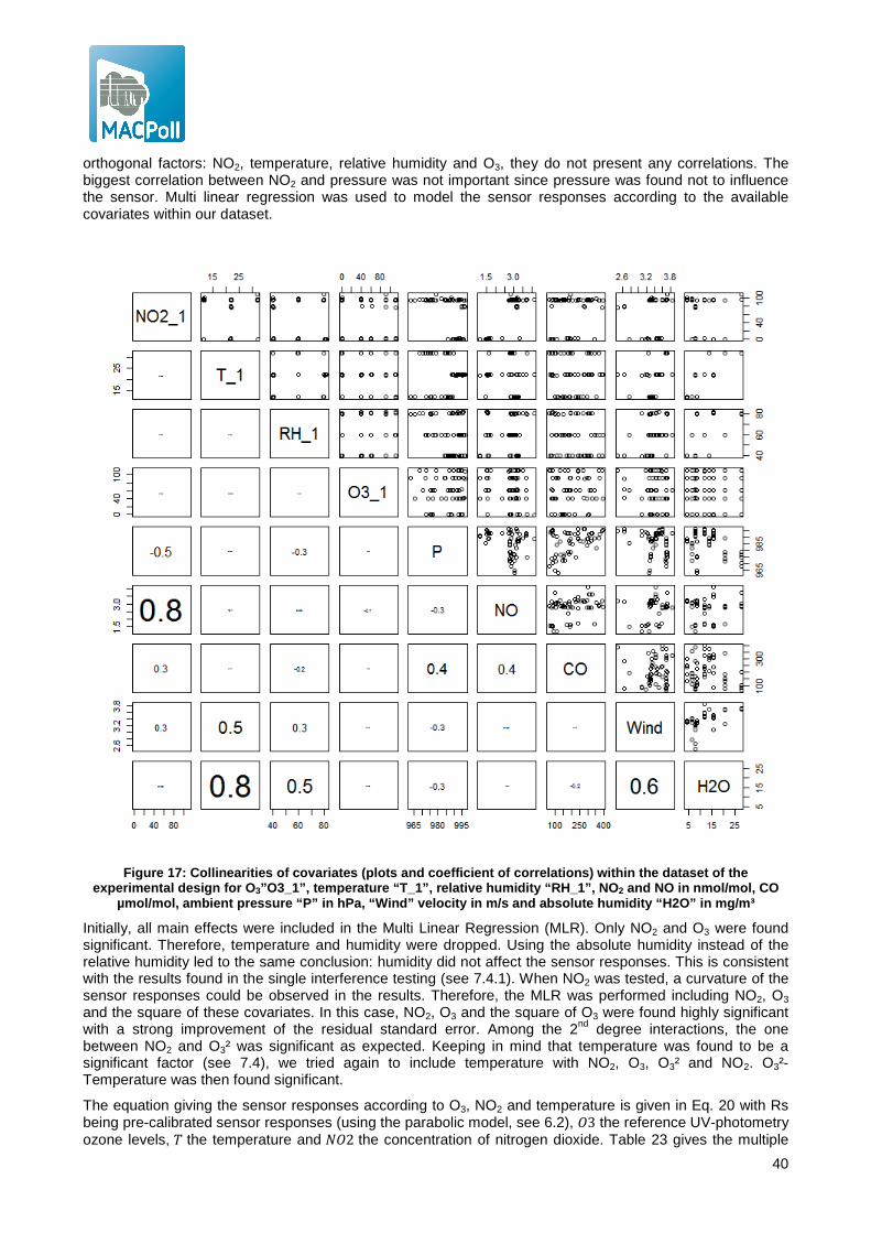
40

orthogonal factors: NO2, temperature, relative humidity and O3, they do not present any correlations. The biggest correlation between NO2 and pressure was not important since pressure was found not to influence the sensor. Multi linear regression was used to model the sensor responses according to the available covariates within our dataset.

Figure 17: Collinearities of covariates (plots and coefficient of correlations) within the dataset of the

experimental design for O 3”O3_1”, temperature “T_1”, relative humidity “RH_1” , NO2 and NO in nmol/mol, CO µmol/mol, ambient pressure “P” in hPa, “Wind” velocit y in m/s and absolute humidity “H2O” in mg/m³

Initially, all main effects were included in the Multi Linear Regression (MLR). Only NO2 and O3 were found significant. Therefore, temperature and humidity were dropped. Using the absolute humidity instead of the relative humidity led to the same conclusion: humidity did not affect the sensor responses. This is consistent with the results found in the single interference testing (see 7.4.1). When NO2 was tested, a curvature of the sensor responses could be observed in the results. Therefore, the MLR was performed including NO2, O3 and the square of these covariates. In this case, NO2, O3 and the square of O3 were found highly significant with a strong improvement of the residual standard error. Among the 2nd degree interactions, the one between NO2 and O3² was significant as expected. Keeping in mind that temperature was found to be a significant factor (see 7.4), we tried again to include temperature with NO2, O3, O3² and NO2. O3²-Temperature was then found significant.

The equation giving the sensor responses according to O3, NO2 and temperature is given in Eq. 20 with Rs being pre-calibrated sensor responses (using the parabolic model, see 6.2), �3 the reference UV-photometry ozone levels, � the temperature and ��2 the concentration of nitrogen dioxide. Table 23 gives the multiple

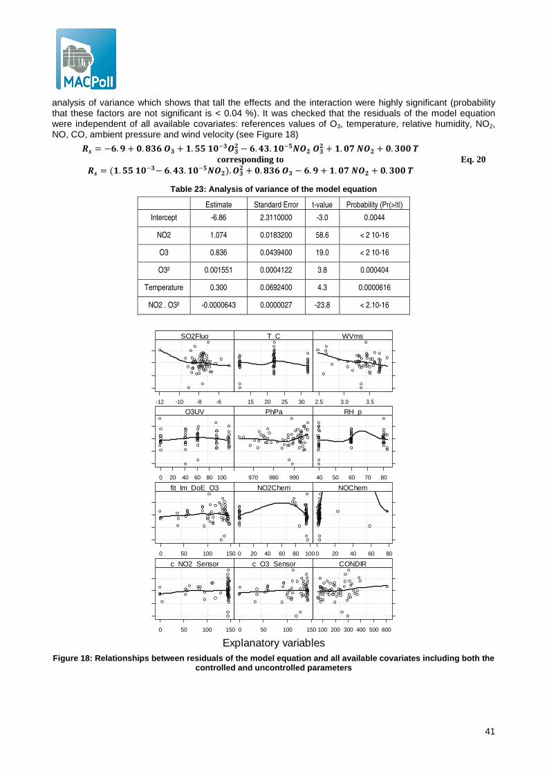
41

analysis of variance which shows that tall the effects and the interaction were highly significant (probability that these factors are not significant is < 0.04 %). It was checked that the residuals of the model equation were independent of all available covariates: references values of O3, temperature, relative humidity, NO2, NO, CO, ambient pressure and wind velocity (see Figure 18)

�� = − .!+ ".#� %� + &.''&"��%�� − .(�.&"�$�%�%�� + &.")�%� + ".�""* corresponding to

�� = (&.''&"��− .(�.&"�$�%�).%�� + ".#� %� − .!+ &.")�%� + ".�""* Eq. 20

Table 23: Analysis of variance of the model equatio n

Estimate Standard Error t-value Probability (Pr(>|t|)

Intercept -6.86 2.3110000 -3.0 0.0044

NO2 1.074 0.0183200 58.6 < 2 10-16

O3 0.836 0.0439400 19.0 < 2 10-16

O3² 0.001551 0.0004122 3.8 0.000404

Temperature 0.300 0.0692400 4.3 0.0000616

NO2 . O3² -0.0000643 0.0000027 -23.8 < 2.10-16

Figure 18: Relationships between residuals of the m odel equation and all available covariates includin g both the

controlled and uncontrolled parameters

Explanatory variables0 50 100 150

c_NO2_Sensor

0 50 100 150

c_O3_Sensor

100 200 300 400 500 600

CONDIR

0 50 100 150

fit_lm_DoE_O3

0 20 40 60 80 100

NO2Chem

0 20 40 60 80

NOChem

0 20 40 60 80 100

O3UV

970 980 990

PhPa

40 50 60 70 80

RH_p-12 -10 -8 -6

SO2Fluo

15 20 25 30

T_C

2.5 3.0 3.5

WVms

42

Table 24: Results of the design of experiments, the sensor results are calibrated with the parabolic m odel

NO2 T RH O3 P NO CO Wind Sensor

nmol/mol °C % nmol/mol hPa nmol/mol nmol/mol m/s nmol/mol

0.7 11.9 60.0 61.1 986.0 1.6 345.3 3.2 55.1

0.4 22.0 40.0 0.3 994.2 1.6 77.8 3.2 0.5

0.4 22.0 40.1 40.9 996.6 1.6 90.9 3.2 36.9

0.5 22.1 40.1 61.2 993.4 1.6 173.0 3.2 60.0

0.4 22.0 40.4 91.8 995.8 1.6 113.5 3.2 93.3

0.4 22.1 40.1 112.4 994.1 1.5 70.1 3.2 109.3

0.8 22.1 59.9 0.4 992.8 2.2 NA 3.7 -0.5

1.1 22.1 60.0 41.0 991.9 1.7 208.4 3.7 36.4

0.9 22.2 60.0 61.2 991.3 1.8 NA 3.7 61.3

0.7 22.1 60.0 91.8 994.1 1.8 NA 3.5 93.7

1.3 22.1 60.0 112.2 992.6 1.7 270.5 3.8 110.9

0.4 21.8 80.0 0.5 995.1 1.6 82.2 3.2 -1.4

0.4 21.9 80.0 41.1 995.1 1.5 84.5 3.2 31.9

0.6 22.0 79.3 61.2 989.0 1.6 195.5 3.2 61.0

0.4 21.9 80.0 92.0 996.0 1.5 85.1 3.2 91.8

0.4 21.8 80.0 112.4 992.5 1.5 87.8 3.1 108.3

0.7 32.1 60.0 61.1 987.2 1.6 342.0 3.5 62.2

97.9 11.9 39.9 1.0 988.2 3.1 189.2 3.3 92.5

96.9 12.0 40.2 40.8 989.1 3.3 298.1 3.3 117.9

96.1 12.0 40.1 61.1 987.6 3.2 251.0 3.3 126.0

96.1 12.0 40.1 91.7 989.3 3.2 240.9 3.3 136.3

95.5 11.7 40.0 112.1 987.1 3.2 131.8 3.3 136.7

95.6 12.0 60.0 0.3 972.8 2.8 144.9 3.3 100.3

98.0 11.8 60.0 40.7 982.0 3.1 354.2 3.4 127.1

94.9 11.9 60.0 61.1 978.0 3.0 187.2 3.3 135.0

96.5 11.9 60.0 91.7 984.6 3.1 112.1 3.4 137.9

94.9 12.0 60.0 112.1 972.9 3.0 163.3 3.3 138.9

95.1 12.0 79.5 1.0 976.1 2.9 149.9 3.3 99.7

94.8 12.0 79.6 40.8 965.4 3.1 101.9 3.3 125.9

95.5 12.0 80.1 60.2 975.6 3.1 227.7 3.3 133.7

94.8 12.0 79.2 91.7 963.1 3.0 120.9 3.3 138.1

95.0 11.9 80.0 112.1 987.1 3.3 271.7 3.3 137.8

83.9 22.1 40.0 0.8 994.9 3.6 198.3 2.6 89.7

80.8 22.0 39.9 41.7 996.5 3.1 278.4 2.6 119.5

79.5 22.0 39.8 62.3 994.8 3.2 79.8 2.6 128.6

78.1 22.1 39.9 90.7 996.7 3.1 281.5 2.6 137.3

76.3 22.1 40.0 112.0 995.0 3.2 386.9 2.5 138.5

96.3 22.1 60.0 1.4 993.3 2.9 212.9 3.6 104.9

94.1 22.2 60.0 40.8 995.6 2.8 394.8 3.6 131.4

94.6 22.3 60.0 60.6 993.5 2.7 323.9 3.8 137.3

93.8 22.1 60.0 91.7 992.5 2.9 371.2 3.6 139.7

94.6 22.1 60.0 110.4 996.8 2.7 242.5 3.6 139.7

43

NO2 T RH O3 P NO CO Wind Sensor

nmol/mol °C % nmol/mol hPa nmol/mol nmol/mol m/s nmol/mol

96.4 22.2 79.9 -0.6 988.8 4.1 304.4 3.4 111.9

95.8 22.1 80.0 40.7 993.4 3.7 329.8 3.4 131.8

94.4 22.0 80.0 61.1 991.7 3.6 311.0 3.4 138.9

96.1 22.1 80.0 91.7 992.9 3.7 309.8 3.4 139.6

94.9 22.1 80.0 112.1 989.9 3.5 240.8 3.4 139.0

95.1 32.0 39.9 -0.4 986.7 2.8 305.4 3.7 103.3

95.0 32.0 40.0 40.8 985.1 2.8 209.3 3.7 129.3

95.0 32.0 39.9 61.1 987.7 2.8 322.0 3.7 136.4

95.0 32.0 39.9 91.7 984.2 2.8 295.4 3.7 139.7

94.9 32.0 40.0 112.0 989.5 2.8 370.3 3.7 140.5

95.0 32.0 60.0 0.5 977.1 2.9 136.6 3.7 110.1

95.0 32.0 60.0 40.7 973.9 2.7 80.0 3.7 132.8

95.0 32.1 60.0 61.2 977.2 2.8 155.4 3.7 138.9

95.0 32.0 60.0 91.7 972.5 2.8 105.2 3.7 139.9

95.0 32.0 60.0 112.1 979.0 2.8 183.6 3.7 140.6

96.1 32.0 79.7 1.0 975.2 3.7 101.0 3.7 109.0

96.5 32.1 80.0 40.7 977.0 3.1 104.3 3.7 131.2

96.2 32.0 80.0 61.1 970.8 2.9 86.6 3.7 139.2

109.3 32.0 80.0 91.9 978.9 2.8 199.3 3.7 141.5

95.9 32.0 80.0 112.1 968.6 2.9 64.2 3.7 139.7

8.1 Uncertainty estimation

Finally, Eq. 20 can be solved to be able to estimate O3, as given in Eq. 22. Obviously, the drawback of this equation is that it uses temperature and more problematic NO2 as well.

%� = −".#� + +".#� � − (,&.''&"�� − .(�&"�$�%�-�&.")�%� + ".�""*− .!− ��.� �%/�&.'''&"�� − .(�&"�$�%�� Eq. 21

0&��%�� = ∑ 1'(�')�

2� 0��3�� and U = k. uc with k = 2 Eq. 22

Which such a complicated model including 9 variables plus a second order polynomial, it would be too complicated to estimate the measurement uncertainty using the GUM method (see Eq. 22). Alternatively, we assume that the variance of the measurement is the sum of the variance of individual random variables including the contributions of the lack of fit of the model equation, NO2 interference, temperature and humidity effect, hysteresis and matrix effect given in Table 25. The following observations apply:

1. The variance of the lack of fit of the model equation was estimated using the residuals of the laboratory model equation (Eq. 20). This parameter already includes contribution from the lack of fit of the calibration, the repeatability of sensor responses, and the short term drift: Hence these parameters are not repeated in the table.

2. In the column where the model equation is applied, the NO2 contribution becomes null since it is corrected for. However, this implied that NO2 has to be measured. Consequently an uncertainty for NO2 measurements shall e considered. The NO2 standard uncertainty was set by difference between the DQO and the rest of the parameter contributions resulting in standard uncertainty of 7.9 nmol/mol (expanded uncertainty U = 15.8 nmol/mol). Conversely, if the sensor values are not

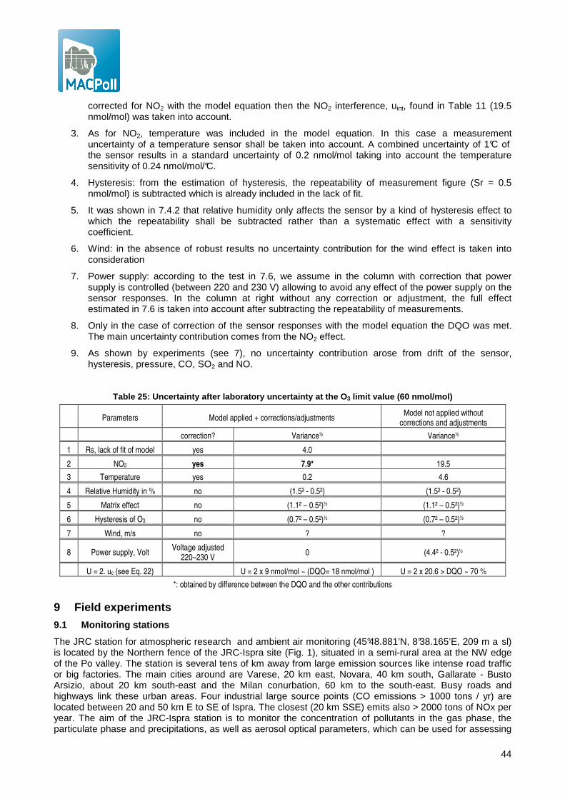
44

corrected for NO2 with the model equation then the NO2 interference, uint, found in Table 11 (19.5 nmol/mol) was taken into account.

3. As for NO2, temperature was included in the model equation. In this case a measurement uncertainty of a temperature sensor shall be taken into account. A combined uncertainty of 1°C of the sensor results in a standard uncertainty of 0.2 nmol/mol taking into account the temperature sensitivity of 0.24 nmol/mol/°C.

4. Hysteresis: from the estimation of hysteresis, the repeatability of measurement figure (Sr = 0.5 nmol/mol) is subtracted which is already included in the lack of fit.

5. It was shown in 7.4.2 that relative humidity only affects the sensor by a kind of hysteresis effect to which the repeatability shall be subtracted rather than a systematic effect with a sensitivity coefficient.

6. Wind: in the absence of robust results no uncertainty contribution for the wind effect is taken into consideration

7. Power supply: according to the test in 7.6, we assume in the column with correction that power supply is controlled (between 220 and 230 V) allowing to avoid any effect of the power supply on the sensor responses. In the column at right without any correction or adjustment, the full effect estimated in 7.6 is taken into account after subtracting the repeatability of measurements.

8. Only in the case of correction of the sensor responses with the model equation the DQO was met. The main uncertainty contribution comes from the NO2 effect.

9. As shown by experiments (see 7), no uncertainty contribution arose from drift of the sensor, hysteresis, pressure, CO, SO2 and NO.

Table 25: Uncertainty after laboratory uncertainty at the O 3 limit value (60 nmol/mol)

Parameters Model applied + corrections/adjustments Model not applied without

corrections and adjustments

correction? Variance½ Variance½

1 Rs, lack of fit of model yes 4.0

2 NO2 yes 7.9* 19.5

3 Temperature yes 0.2 4.6

4 Relative Humidity in % no (1.5² - 0.5²) (1.5² - 0.5²)

5 Matrix effect no (1.1² – 0.5²)½ (1.1² – 0.5²)½

6 Hysteresis of O3 no (0.7² – 0.5²)½ (0.7² – 0.5²)½

7 Wind, m/s no ? ?

8 Power supply, Volt Voltage adjusted

220–230 V 0 (4.4² - 0.5²)½

U = 2. uc (see Eq. 22) U = 2 x 9 nmol/mol ~ (DQO= 18 nmol/mol ) U = 2 x 20.6 > DQO ~ 70 %

*: obtained by difference between the DQO and the other contributions

9 Field experiments

9.1 Monitoring stations

The JRC station for atmospheric research and ambient air monitoring (45°48.881’N, 8°38.165’E, 209 m a sl) is located by the Northern fence of the JRC-Ispra site (Fig. 1), situated in a semi-rural area at the NW edge of the Po valley. The station is several tens of km away from large emission sources like intense road traffic or big factories. The main cities around are Varese, 20 km east, Novara, 40 km south, Gallarate - Busto Arsizio, about 20 km south-east and the Milan conurbation, 60 km to the south-east. Busy roads and highways link these urban areas. Four industrial large source points (CO emissions > 1000 tons / yr) are located between 20 and 50 km E to SE of Ispra. The closest (20 km SSE) emits also > 2000 tons of NOx per year. The aim of the JRC-Ispra station is to monitor the concentration of pollutants in the gas phase, the particulate phase and precipitations, as well as aerosol optical parameters, which can be used for assessing

45

the impact of European policies on air pollution and climate change. Measurements are performed in the framework of international monitoring programs like the Co-operative program for monitoring and evaluation of the long range transmission of air pollutants in Europe (EMEP) of the UN-ECE Convention on Long-Range Transboundary Air Pollution (CLRTAP) and the Global Atmosphere Watch (GAW) Program of the World Meteorological Organization (WMO).

From May 2012 until October 2012, a mobile laboratory was installed near the EMEP station sited at Ispra, equipped with routine analysers normally installed in the containers. Gases were sampled using a sampling line (see Figure 19) placed at the top of the roof of the van at about 3.5 m above the ground and on the roof of the mobile laboratory. The sampling line consists in a stainless steel gas inlet with grid protection for rain, insects and dust. The stainless steel inlet tube of 4 cm internal diameter with internal PTFE tube that ends with a Teflon manifold of 8 PTFE ports to connect the gas analysers. The sampling line is flushed with ambient air with about 2 second resident time of samples. Each instrument samples from the glass tube with its own pump through a ¼” PTFE/PFE tube and a 1 µm pore size 47 mm diameter Teflon filter to eliminate particles from the sampled air.

The mobile laboratory was equipped with meteorological sensors and gas analysers which were calibrated in laboratory before the in-situ measurements and then checked every month. Field checks were carried out using zero air in gas cylinders and a span value (internally certified gas cylinders at low concentration for NO/NOx and SO2, highly concentrated cylinders for CO and ozone generator do O3). The highest observed drift of calibration was 3 %, consistent with the uncertainty of the working standards used on field. Therefore, no correction of measurements was undergone apart from the discarding values during maintenance and calibration checks.

• Meteorological parameters (ambient temperature, ambient relative humidity, ambient pressure, 10m mast for wind speed and wind direction) a mobile. The mobile laboratory was equipped with:

• Gaseous pollutants: for O3 an UV Photometric Analyzer Thermo Environment 49C; for NO2/NO/NOx a Chemiluminescence Nitrogen Oxides Analyzer Thermo 42C; for CO a non-Dispersive Infrared Gas-Filter Correlation Spectroscopy Thermo 48C-TL, for SO2 and UV Fluorescent Analyser Thermo 43C TL

Figure 19: mobile laboratory used that the EMEP statio n of JRC Ispra.

Sensors Meteorological mast

Inlet sampling

line

46

9.2 Sensor equipment

To avoid interference, we made sure that the flow air coming out of the air condition system was blowing far enough from the sensor to avoid any effect on the sensor responses.

Figure 20 Sensors location at the monitoring station

9.3 Check of the sensor in laboratory

Hopefully, the sensor should have been tested in laboratory before installation in field. However, the exposure chamber was busy with the laboratory tests when receiving the field sensor and the laboratory check had to be postponed to the end of the field experiment. Consequently, the field sensor was submitted to a lab tests at the end of the field experiment as described in 7.3. During experiment, NO2, temperature and humidity were kept under control. The temperature and relative conditions of the test were set at 22°c and 60 % of relative humidity, the defined mean values.

The results of the experiment are given in Figure 1 which shows that little or no curvature of the field sensor responses, conversely to what was observed for the lab sensor (6.2). A simple linear equation was sufficient for this sensor. Consequently, it was expected that the field sensor would give a linear response during the field experiment.

The pre-calibration functions were established by plotting sensor responses versus reference values measured by the TECO 49C analyser (see Figure 6) of relative humidity. Each steps lasted for 150 minutes once the condition of O3 concentrations, temperature and humidity were reached. The averages of the last 60 minutes were plotted. For the field experiment, the calibration functions established in this tests was not systematically applied.

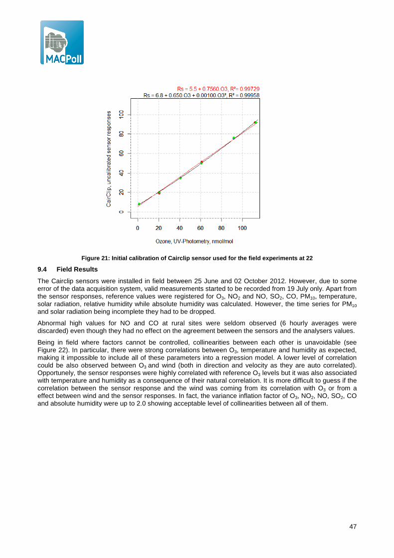
47

Figure 21: Initial calibration of Cairclip sensor u sed for the field experiments at 22

9.4 Field Results

The Cairclip sensors were installed in field between 25 June and 02 October 2012. However, due to some error of the data acquisition system, valid measurements started to be recorded from 19 July only. Apart from the sensor responses, reference values were registered for O3, NO2 and NO, SO2, CO, PM10, temperature, solar radiation, relative humidity while absolute humidity was calculated. However, the time series for PM10 and solar radiation being incomplete they had to be dropped.

Abnormal high values for NO and CO at rural sites were seldom observed (6 hourly averages were discarded) even though they had no effect on the agreement between the sensors and the analysers values.

Being in field where factors cannot be controlled, collinearities between each other is unavoidable (see Figure 22). In particular, there were strong correlations between O3, temperature and humidity as expected, making it impossible to include all of these parameters into a regression model. A lower level of correlation could be also observed between O3 and wind (both in direction and velocity as they are auto correlated). Opportunely, the sensor responses were highly correlated with reference O3 levels but it was also associated with temperature and humidity as a consequence of their natural correlation. It is more difficult to guess if the correlation between the sensor response and the wind was coming from its correlation with O3 or from a effect between wind and the sensor responses. In fact, the variance inflation factor of O3, NO2, NO, SO2, CO and absolute humidity were up to 2.0 showing acceptable level of collinearities between all of them.

48

Figure 22: Collinearities in the field data set wit h scatterplots between pairs of parameters (upper m atrix plots)

and their correlation (lower matrix values) for hou rly values of O 3, NO2, NO, and SO2 in nmol/mol, CO in µmol/mol, temperature in °C (T), relative humidity in % (RH), absolute humidity in mg/m³ (H2O), wind d irection in

° (WD), wind velocity in m/s (WV) and pressure in hPa (P). O3.

Subsequently different treatment was applied to the sensor responses which were plotted against the reference O3 measured by UV photometry. Figure 23 shows in order of appearance:

1. Raw sensor responses against reference O3: the response are highly linear with high coefficient of determination (R² = 0.917) but with a slope and interception of the regression line different from 1 and O, respectively. A few abnormal values appears towards 40 nmol/mol.

2. Sensor responses after calibration using the pre-calibration function established in laboratory (see 9.3), both the agreement between the sensor and UV-photometry improved with the slope increasing from 0.45 to 0.65, the intercept decreasing from 7.4 to 1.5 and a slight increase of the coefficient of determination. Nevertheless the slope being different from 1, this shows that laboratory calibration does not ensure full agreement between sensor responses and UV photometry in field.

3. Application of the laboratory model (Eq. 21) to the sensor response calibrated with the laboratory calibration function did not improve further the data: the slope only slightly improves (0.68 instead of 0.65) but the coefficient of determination slightly worsened (0.89 instead of 0.92). In fact the model was designed for both high levels of O3 and NO2 while only low levels of NO2 were registered during the field campaign. The manufacturer gave this information: because of the electrolyte, electrochemical sensors need a minimum humidity in the atmosphere. Low humidity can lead to a diminution of the electrolyte

49

volume and consequently to an increase of the signal which is proportional to its concentration in the electrolyte.

On the plots 1 to 3 of Figure 23, a few abnormal peak values appeared at about 40 nmol/mol of O3. Generally, they demonstrated homogeneity of variance between the residuals and the fitted variables (fit_lm_Field_O3) apart from the peak values at 40 nmol/mol. In order to investigate these values, a linear line was fitted between the sensor responses and the reference O3. The residuals of this linear model were plotted against all covariates (see Figure 24). It appeared that the high residuals values were associated with low values of humidity (relative and absolute), NO and NO2, SO2 and CO and high wind velocities. The sole causality relation that we could find was that at low relative humidity, the cellulose buffer used for adjusting the relative humidity of the sensor may not be effective and hence disturbing the sensor correct operation. It was thus decided to discard the sensor values when relative humidity was < 35 %.

4. Calibration of the sensor responses versus reference O3 during the 1st week of measurements. 5. Sensor responses from the 2nd week of the measuring campaign versus reference O3 with relative

humidity < 35 % discarded. The sensor is calibrated on field during the 1st week of the field campaign by comparison to the UV-photometry analyser.

6. The same treatment as in plot 5 adding the application of the model equation (Eq. 21) established in the laboratory. A little improvement occurs that maybe not worth since temperature and NO2 were needed. It is possible that in situation where high NO2 and O3 are registered, the model equation would have been more effective.

1 2

50

Figure 23: Sensor responses versus O 3 reference values. Upper left: raw sensor responses ; upper right: laboratory calibrated sensor responses; middle left : laboratory calibrated sensor responses and applic ation of

the laboratory model equation; middle right: calibr ation during the 1 st week of measurement; Bottom left: sensor responses from the 2 nd week of the campaign, field calibrated with data o f the 1 st week, without values with

relative humidity < 35 %; Bottom right the same as bottom left with application of the laboratory mode l equation.

3 4

5 6

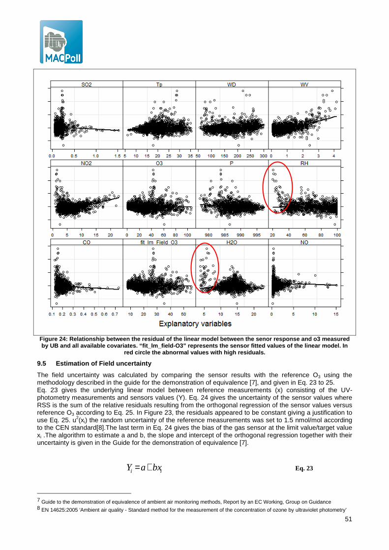
51

Figure 24: Relationship between the residual of the linear model between the senor response and o3 mea sured by UB and all available covariates. “fit_lm_field-O 3” represents the sensor fitted values of the linea r model. In

red circle the abnormal values with high residuals.

9.5 Estimation of Field uncertainty

The field uncertainty was calculated by comparing the sensor results with the reference O3 using the methodology described in the guide for the demonstration of equivalence [7], and given in Eq. 23 to 25. Eq. 23 gives the underlying linear model between reference measurements (x) consisting of the UV-photometry measurements and sensors values (Y). Eq. 24 gives the uncertainty of the sensor values where RSS is the sum of the relative residuals resulting from the orthogonal regression of the sensor values versus reference O3 according to Eq. 25. In Figure 23, the residuals appeared to be constant giving a justification to use Eq. 25. u2(xi) the random uncertainty of the reference measurements was set to 1.5 nmol/mol according to the CEN standard[8].The last term in Eq. 24 gives the bias of the gas sensor at the limit value/target value xi .The algorithm to estimate a and b, the slope and intercept of the orthogonal regression together with their uncertainty is given in the Guide for the demonstration of equivalence [7].

ii bxaY +=

Eq. 23

7 Guide to the demonstration of equivalence of ambient air monitoring methods, Report by an EC Working, Group on Guidance 8 EN 14625:2005 ‘Ambient air quality - Standard method for the measurement of the concentration of ozone by ultraviolet photometry’

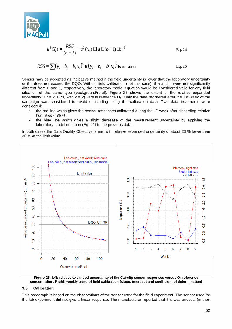
52

222 ])1([)()2(

)( iii xbaxun

RSSYu ⋅−++−

−= Eq. 24

( )∑ −−= 210 ii xbbyRSS if ( )2

10 ii xbby −− is constant Eq. 25

Sensor may be accepted as indicative method if the field uncertainty is lower that the laboratory uncertainty or if it does not exceed the DQO. Without field calibration (not this case), if a and b were not significantly different from 0 and 1, respectively, the laboratory model equation would be considered valid for any field situation of the same type (background/rural). Figure 25 shows the extent of the relative expanded uncertainty (Ur = k. u(Yi) with k = 2) versus reference O3. Only the data registered after the 1st week of the campaign was considered to avoid concluding using the calibration data. Two data treatments were considered:

• the red line which gives the sensor responses calibrated during the 1st week after discarding relative humilities < 35 %.

• the blue line which gives a slight decrease of the measurement uncertainty by applying the laboratory model equation (Eq. 21) to the previous data.

In both cases the Data Quality Objective is met with relative expanded uncertainty of about 20 % lower than 30 % at the limit value.

Figure 25: left: relative expanded uncertainty of t he Cairclip sensor responses versus O 3 reference concentration. Right: weekly trend of field calibra tion (slope, intercept and coefficient of determina tion)

9.6 Calibration

This paragraph is based on the observations of the sensor used for the field experiment. The sensor used for the lab experiment did not give a linear response. The manufacturer reported that this was unusual (in their

53

experience, the sensor is linear). Anyhow all conclusions drawn from the field sensor could be applied to any sensor provided that its response is made linear using for example a laboratory calibration.

The sensor used at the field site was not previously calibrated by the manufacturer at reception.

1. During the field experiment, the sensor was found linear. The calibration function was: Rs = 7.4 + 0.457 O3 where O3 was reference values measured by UV-photometry.

2. In laboratory, the sensor showed a linear relationship. However, the calibration function was different than the one observed in field: Rs = 5.5 + 0.756 O3 (see 9.3). The manufacturer argued that this difference was the result of an exceptional conditioning problem. However, three replicated calibrations in the laboratory gave the same calibration function. The application of the laboratory model equation (Eq. 21) did not produce better agreement with UV-photometry in this case.

3. Conversely, it was observed that the sensor responses of 10 weeks of field measuring campaign could agree with UV-photometry provided that the sensor was calibrated during the 1st week of comparison sensor versus UV-photometry.

4. Once the sensor was calibrated during the 1st week, provided that this period included the whole range of O3 conditions, the sensor was shown to keep on agreeing with UV-photometry for 10 weeks. The application of the laboratory model equation (Eq. 21) led to slight improvements while temperature and NO2 were needed in the model equation. NO2 was very low during the field experiment; it is possible that if it was higher the model equation would have been more effective.

5. Re-calibration was not found necessary during the whole field campaign since the calibration function did not show any trend both in the laboratory and field experiments. Some random noise in these data cannot be avoided because of the timely change of concentration levels. The re-calibration periodicity can be set to the whole duration of the field campaign: 1+9 weeks.

Our observation was that calibration of the sensor shall be carried out during field experiment by comparison to reference measurements. It is likely that the validity of this observation is limited to the monitoring site of the field experiment. .

The figure next page presents the trend of the sensor responses in nmol/mol calibrated during the 1st week without relative humidity lower than 35 %. The figure also shows reference O3 in nmol/mol, temperature in °C and relative humidity in %.

54

0

20

40

60

80

100

29-Jul 8-Aug 18-Aug 28-Aug 7-Sep 17-Sep 27-Sep

O3 NO2 Tp fit_lm_Field_O3

55

10 Conclusions

The main advantages of CairclipO3/NO2 sensor compared to other sensor were that it did not suffer long term drift and that it was free from humidity effect. This was confirmed during the field experiment provided that relative humidity did not reach too low values (RH < 35 %).

The CairclipO3/NO2 is designed to measure both O3 and NO2. When monitoring the sole O3, the major drawback of the sensor is its sensitivity to NO2 that may prevent from correctly estimating O3 if high levels of NO2 and O3 are simultaneously present in the sampled air. In this study it was decided to evaluate the sensor at sites where NO2 and O3 are not simultaneously at high levels namely background sites at rural areas.

In laboratory, a number of experiments showed that the sensor is in fact highly sensitive to NO2 but is independent from change of CO, NO, CO2 and NH3. The sensor did not undergo short and long term drift, it was not sensitive to pressure changes and did not present hysteresis effect when ozone changes. It was slightly dependent to temperature and power supply changes that needs to be controlled. It showed little hysteresis when relative humidity changes. Some doubts remain about the sensitivity of the sensor to wind velocity.

A sophisticated model equation was established in laboratory that needs NO2 and temperature to estimate O3. In laboratory and at high NO2 levels, when using this model the measurement uncertainty was found lower that the Data Quality Objective of the European Directive for measurement while the DQO would not be met without.

However, the effectiveness of the laboratory model equation was not easily demonstrated with the results of the field campaign for several reasons. Firstly, the calibration function of the field sensor was nearly linear while the one of the laboratory was clearly parabolic. The manufacturer suggested that this difference might be the result of different conditioning effect of the sensor during this study. Secondly, the laboratory model equation was designed to improve the sensor responses in case of high NO2 levels. However, the measuring campaign took place at rural areas and in summer when O3 levels are high with low NO2 levels. In this case, the Cairclip sensor showed a linear response without applying the laboratory model equation which could not further improve the sensor agreement with the UV-photometry method. It would be interesting to estimate the efficiency of the model equation when NO2 is higher.

Conversely to the manufacturer experience, our observation was that the Cairclip sensor could not only rely on the calibration carried out in laboratory model nor a simple adjustment. A field calibration of one week was found effective for a 10-week period of used. Both in laboratory and in field, it was found that re-calibration of the sensor was not necessary over a 10-week measuring campaign.

The Data Quality Objective of indicative method of the European Directive is met by the CairClipO3/NO2. In fact, at the limit value of 60 nmol/mol, the relative expanded uncertainty of the sensor measurements was found to be about 20 % while the DQO is 30 %. Applying the laboratory model equation only improved the relative expanded uncertainty to 19 %.

Since, the laboratory model equation resulted in a high bias when used in field measurement and that the sensor needed to be calibrated for field use, it is advised to confirm the sensor measurement by comparison to the UV-photometry method.

Further to this study, the field of application of the Cairclip sensor is validated for fixed measurement at background site/rural areas provided that the sensor is calibrated by comparison to the UV-photometry method before normal use.

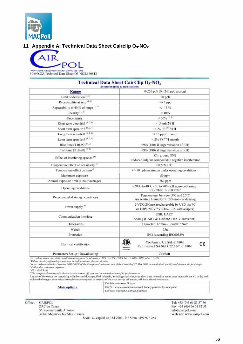
56

11 Appendix A: Technical Data Sheet Cairclip O 3-NO2

57

12 Appendix B: Response time steps

58

European Commission

EUR 26373 – Joint Research Centre – Institute for Environment and Sustainability

Title: Report of laboratory and in-situ validation of micro-sensor for monitoring ambient air pollution

Author(s): Laurent Spinnelle, Michel Gerboles and Manuel Aleixandre

Luxembourg: Publications Office of the European Union

2013 – 59 pp. – 21.0 x 29.7 cm

EUR – Scientific and Technical Research series – ISSN 1831-9424 (online)

ISBN 978-92-79-34832-7 (pdf)

doi: 10.2788/4277

Abstract

The aim of this report is to evaluate and validate CairClipO3/NO2 sensors of CAIRPOL with laboratory and field tests under

ambient/indoor air conditions corresponding to a specific micro-environment: background station, rural areas. This report presents

the evaluation of the performances of the sensor and the determination of its laboratory and field measurement uncertainty

compared to the Data Quality Objective (DQO) of the European Air Quality Directive for indicative method. Further, procedures

for the calibration of sensors able to ensure full traceability of measurements of sensors to SI units are developed.

59

z

As the Commission’s in-house science service, the Joint Research Centre’s mission is to provide EU policies with independent, evidence-based scientific and technical support throughout the whole policy cycle. Working in close cooperation with policy Directorates-General, the JRC addresses key societal challenges while stimulating innovation through developing new standards, methods and tools, and sharing and transferring its know-how to the Member States and international community. Key policy areas include: environment and climate change; energy and transport; agriculture and food security; health and consumer protection; information society and digital agenda; safety and security including nuclear; all supported through a cross-cutting and multi-disciplinary approach.

LB-N

A-2

6373-E

N-N

report of laboratory and in -situ validation of micro...

Documents