research and development of a land use scenario modeling …
TRANSCRIPT
Portland State University Portland State University
PDXScholar PDXScholar
Urban Studies and Planning Faculty Publications and Presentations
Nohad A. Toulan School of Urban Studies and Planning
5-2013
Research and Development of a Land Use Scenario Research and Development of a Land Use Scenario
Modeling Tool Modeling Tool
John Gliebe Portland State University
Hongwei Dong Portland State University
Josh Frank Roll Portland State University, [email protected]
Follow this and additional works at: https://pdxscholar.library.pdx.edu/usp_fac
Part of the Transportation Commons, Urban Studies Commons, and the Urban Studies and Planning
Commons
Let us know how access to this document benefits you.
Citation Details Citation Details Gliebe, John; Dong, Hongwei; and Roll, Josh Frank, "Research and Development of a Land Use Scenario Modeling Tool" (2013). Urban Studies and Planning Faculty Publications and Presentations. 142. https://pdxscholar.library.pdx.edu/usp_fac/142
This Report is brought to you for free and open access. It has been accepted for inclusion in Urban Studies and Planning Faculty Publications and Presentations by an authorized administrator of PDXScholar. Please contact us if we can make this document more accessible: [email protected].
RESEARCH AND DEVELOPMENT OF A LAND USE SCENARIO
MODELING TOOL
Interagency Agreement 24620
Work Order Contract #6
Prepared by:
John Gliebe
Hongwei Dong
Joshua Roll
Center for Urban Studies
Portland State University
P.O. Box 751 USP
Portland, OR 97207-0751
For
Oregon Department of Transportation
Transportation Planning Analysis Unit
555 13th
St SE, Suite 2
Salem, Oregon 97310
May 2013

Table of Contents
Table of Contents ............................................................................................................................ 2
Background ..................................................................................................................................... 4
Study Objectives and Outcomes ................................................................................................. 4
Summary of Accomplishments ................................................................................................... 5
Remainder of Document ............................................................................................................. 6
Strengths and Weaknesses of LUSDR ............................................................................................ 7
1. Land Price Model Enhancements ............................................................................................ 9
Hedonic Land Price and Densification Models .......................................................................... 9
Implementation Issues .............................................................................................................. 13
2. Splitting Development Types ................................................................................................ 15
Summary of Findings on Forecasting Methods ........................................................................ 15
3. Land Fragmentation Procedure ............................................................................................. 17
Data and Method ....................................................................................................................... 17
Implementation and Integration into LUSDR........................................................................... 20
Comparison of Base Scenario with Scenario Including landFrag Function ............................ 21
4. Fixed Development Types ..................................................................................................... 30
Proposed Approach ................................................................................................................... 30
Implementation Issues .............................................................................................................. 32
5. Endogenously Determined Employment Mix ....................................................................... 33
Commercial Development Location Choice Model ................................................................. 34
Implementation Issues .............................................................................................................. 38
6. Evaluation of Transferability ................................................................................................. 39
Development and Testing Activities ......................................................................................... 39
General Findings ....................................................................................................................... 40
Sensitivity Testing .................................................................................................................... 40
Recommendations ..................................................................................................................... 41
7. Data for Transferability ......................................................................................................... 43
8. Streamlined Travel Demand Model ...................................................................................... 44
9. Visualization Tools and Evaluation of Model Outputs ......................................................... 45
10. Zoning Allocation .............................................................................................................. 46
Descriptive Analysis ................................................................................................................. 46

Center for Urban Studies Portland State University
3
Two-Step Rezoning Allocation Model ..................................................................................... 47
Implementation Issues .............................................................................................................. 53
Further Research and Development Needed............................................................................. 53
11. Housing Type Choice ........................................................................................................ 54
Housing Demand Model ........................................................................................................... 55
Housing Project Synthesis Model ............................................................................................. 61
Housing Project Location Choice Model .................................................................................. 67
Implementation Issues .............................................................................................................. 71
12. Development Degradation and Redevelopment ................................................................ 72
Proposed Algorithm .................................................................................................................. 72
Implementation Issues .............................................................................................................. 73
Appendix A ................................................................................................................................... 75
Appendix B ................................................................................................................................... 78

Center for Urban Studies Portland State University
4
Background
Oregon Department of Transportation’s (ODOT) Transportation Planning and Analysis Unit
(TPAU) developed a land use modeling tool called the “Land Use Scenario Developer in R”
(LUSDR). LUSDR is a modeling tool, written in the “R” language, that may be used to predict
and analyze regional land use changes probabilistically, creating a distribution of possible
outcomes. It is designed to be integrated with travel demand modeling programs, making it
potentially valuable for analyzing the interaction between transportation and land use when
assessing various growth-policy and socioeconomic assumptions.
Among known land use modeling tools, LUSDR represents a unique approach. By design,
LUSDR utilizes Monte Carlo simulation methods to predict a range of possible outcomes for a
given set of inputs, rather than a single outcome (point estimate). It can thus be used to analyze
the potential impacts of transportation system changes and policy scenarios on land use, with the
distribution of outcomes forming a “risk profile.”
The prototype application of LUSDR was created for the Medford area and was reviewed by a
panel of peer experts in integrated modeling methods. The peer review panel gave overall
approval to the use of LUSDR, its structure, and algorithms, but also identified several areas that
needed improvement. Before LUSDR is ready for widespread use in transportation planning in
other regions, the peer review panel recommended that ODOT address certain deficiencies in the
mode design itself and study and support its transferability to regions other than Medford.
ODOT’s original intended use for LUSDR was to provide a tool for systematically and
consistently forecasting land use change by transportation analysts within TPAU, ODOT
regional planners, and analytic planners at MPOs and small urban areas throughout Oregon.
Study Objectives and Outcomes
This project is Phase 2 for Research and Development of a Land Use Scenario Modeling Tool. It
is intended to address several extant deficiencies in the LUSDR modeling tool, each identified
below, as a separate research task. The original proposed outcomes of this research were a set of
programs, data, and documentation that would comprise a deployable LUSDR package.
This ultimate objective—a deployable LUSDR package—was not achieved through this research
project, as stumbling blocks encountered along the way proved too difficult for the study team to
overcome during the period of funding. The primary difficulty was programming. In addition,
the project P.I. and the two graduate students who worked on this project were new to the ‘R’
language, prior to beginning the work, and the LUSDR program source code was not well
documented, either through an external guide or embedded comments. Consequently, a large
amount of time was spent understanding the source code, which led to lengthy “learning curves”
and difficulty when attempting to insert new or modified procedures. In addition, some of the
tasks originally specified under this project, namely development of streamlined travel demand
model to accompany LUSDR and the development of a graphic user interface (GUI) required a
level of ‘R’ programming expertise beyond that possessed by the study team.
Another reason that hampered the development of a deployable LUSDR package was the
architecture of the original program itself. A number of the proposed solutions to the deficiencies
would only work if more sweeping changes to the overall program design were made and were
Center for Urban Studies Portland State University
5
viewed by the study team as “risky” and best left to Brian Gregor of ODOT-TPAU, the
program’s creator, to decide whether and what methods to implement.
Summary of Accomplishments
This research project made progress in providing insights to some of the deficiencies that it was
originally intended to address. Some noteworthy research derived from this study was published
through conference presentations and a journal paper. Below is a list of the twelve tasks specified
under this work order, with a brief description of what was accomplished, explanations for things
that were not accomplished, and in some cases recommendations.
1. Land Price Model Enhancements – The objective of this task was to develop a land
pricing model in which land values rise as a function of density. We estimated various
hedonic pricing models, and derived an initial specification for further testing.
2. Splitting Development Types – The objective of this task was to develop a mechanical
procedure to split a large development cluster into smaller clusters in cases where there
was insufficient vacant land in any single zone to site it. The study team opted instead to
conduct a more scientific comparison of different methods of forecasting development
units. We developed models of the choice of developers to locate new housing stock
using both a development cluster approach and an “atomized” approach (unit-by-unit). A
paper derived from this work was published in Transportation Research Record and
included herein in Appendix B.
3. Land Fragmentation Procedure – The objective of this task was to account for the fact
that the total amount of land available for development within a zone is unlikely to be
contiguous, with smaller fragments more likely with increased urbanization. We
developed a procedure that would predict the probability of finding an available fragment
of land that satisfies a minimum size input criteria, given the degree of development
within zone. The procedure was implemented in R code, tested, and found to work well.
Documentation is provided.
4. Fixed Development Types – The objective of this task was to develop a module to
account for land uses that are better modeled as fixed development types, independent of
market control, such as public facilities, sports stadiums, tourist attractions and similar
uses. We have outlined an approach and recommended a data structure for
implementation.
5. Endogenously Determined Employment Mix – The objective of this task was to create
an employment location choice model. Using Portland regional data, we created four
versions of a commercial development cluster location choice model.
6. Evaluation of Transferability – The objective of this task was to study the transferability
of LUSDR in a region other than Medford, and Mid-Willamette COG was identified as
the case study. ODOT provided LUSDR to MWVCOG, which did attempt an
implementation and provided some initial observations and notes based on their
experience. These are included herein. PSU was to provide assistance as needed and to
study the results; however, this effort never got off the ground due to time and resource
constraints.

Center for Urban Studies Portland State University
6
7. Data for Transferability – The objective of this task was to write a general technical
guide on the methods used and recommended for culling and manipulating the data for
model construction, in part based on the MWVCOG. As the work with MWVCOG was
not completed, neither was this task. To be truly useful, this task would have required a
very in-depth consideration of all aspects of the LUSDR algorithms, R code and data
structures, and how they could be generalized. Thus, it would have to include not only a
data processing manual, but also recommendations for recoding some of the “hardcoded”
elements of the LUSDR program that made it less transferable to other regions.
8. Streamlined Travel Demand Model – The objective of this approach was to create “lite”
version of JEMnR. We did not undertake this task. Since there are many ways that one
could streamline a 4-step model (e.g. fix mode choice, run assignment without feedback,
combine market segments, etc.), this could be a fairly lengthy exercise in its own right.
9. Visualization Tools and Evaluation of Model Outputs – The objective of this task was
to develop a front-end GUI and output data summary and visualization tools. We did not
undertake this task. This would have been a very time-consuming exercise for the entry-
level programming expertise of the study team, but something that more experienced
programmers could do far more efficiently.
10. Zoning Allocation – The objective of this task was to develop a model that would predict
changes to zoning designations. It was not entirely clear to the study team whether this
should actually enter the model as an exogenous policy event, or if we should attempt to
mode it. In the end, we did develop a two-step model that predicts the occurrence of re-
zoning from rural land use to a developable state and, if so, how many acres are
converted. Models were created for both residential and non-residential conversions.
11. Housing Type Choice – The objective of this task was to replace the tree-classification
process with a discrete choice model of housing type choice. We developed a 3-step
process for estimating (1) total housing demand for the region; (2) formation of housing
development clusters (SF, MF), and (3) housing type choice for various household types.
12. Development Degradation and Redevelopment – The objective of this task was to reflect
the possibility of redevelopment, which necessitates simulating the degradation of
buildings over time. The structure of LUSDR poses several challenges to this, such as the
inability to track individual developments, households or employment over time, as well
as the lack of a land price model (see Task 1). We proposed an algorithm to model
development degradation and redevelopment potential, as well as additional
implementation steps that would be needed to support it.
Remainder of Document
In the remainder of this document, we discuss the strengths and weaknesses of the LUSDR
program. This is followed by separate major sections covering each of the tasks summarized
above.
Center for Urban Studies Portland State University
7
Strengths and Weaknesses of LUSDR
The LUSDR model is well suited to providing a quick land use development scenario tool for a
given set of inputs. Its primary strengths are faithful representation of a plausible distribution of
future land use outcomes, based on the continuation of past market trends and public policies.
LUSDR is much more than a trend-analysis tool, however. It is applied in a stochastic
framework, which permits a range of alternative futures through the repeated simulation of
outcomes, and these simulations can be run very quickly. The resulting distribution of outcomes
provides decision makers with a range of plausible outcomes for a given scenario, some of which
will differ significantly from each other. These outcomes may then be used to study the potential
“best” and “worst” cases for the various transportation investment alternatives. This should
prove useful to decision makers in smaller cities whose chief concerns are slow to moderate
growth and modest, incremental infrastructure development. A full description of LUSDR may
be found in the documentation produced by Gregor (2006) of ODOT-TPAU.
LUSDR’s primary limitation is that it is based on statistical associations, with very little in the
way of economic or behavioral models. In large part, this is driven by the objective of producing
many simulated scenarios quickly. LUSDR’s current specification implicitly assumes the
continuation of past economic and regulatory policies and market stability. The model implicitly
maintains constant relationships between the relative values of residential and commercial land,
construction costs, and the rate at which local and state governments will control the pace of
development through investment in non-transportation-related infrastructure (e.g., water and
sewer, schools, energy). It also assumes a constant relationship between household income levels
and rates of consumption on housing, transportation, and consumer goods. The ratio of workers
to jobs and employment by industrial sector are also assumed to remain constant, which implies
that the regional employment levels and mix of industries will continue and that industrial
productivity will remain flat. These assumptions of constancy and lack of a behavioral
foundation limit LUSDR’s usefulness for the analysis of policies that might alter these
relationships, such as policies that would constrain or increase the supply of developable land
and other development management policies, sharp increases in fuel prices, tolling and transit
costs, and travel demand management policies.
Spatially, LUSDR implicitly assumes that land and building values of a specific development
types may be represented by an observed median value, regardless of location within the
urbanized region. Unlike other land use models, that allocate households, employment and floor
space in continuous or elemental units, LUSDR creates and sites development clusters, which is
arguably more realistic. The pitfall of this approach is that it is more difficult to forecast
accurately, leading to greater errors due to “lumpiness.” LUSDR compensates for forecasting
inaccuracy by compelling the analyst to run multiple scenarios and consider the distribution of
outcomes. This may average out to produce expected values very similar to the result if a single
forecast were made using the more common continuous or “atomized” approach; however, by
maintaining these separate scenarios, LUSDR retains more information about the best and worst
cases. On the balance, this is seen as an advantage.
LSUDR also assumes that the development types offering the highest bid for the available space
will locate there, reflecting the traditional economic bid-rent curve. As implemented, this
becomes more of a “tie-breaker” where the queuing of developments for potential siting allows a

Center for Urban Studies Portland State University
8
zone to “fill up” and, only when there is competition for space, does the bid price offered by a
particular development come into play. These areas will be more densely developed if the
underlying zoning allows it. LUSDR does not, however, allow for product differentiation within
the real estate market, so the same per unit prices and land consumption quantities prevail,
regardless of densification. Mixed use developments are also not represented in the current
specification. Further, LUSDR does not allow the possibility of redevelopment, thus it would not
be useful for regions experiencing high growth pressure with a limited supply of vacant land.
Modeling redevelopment in LUSDR is an additional challenge, because it currently does not
track individual development clusters once they are located in a TAZ. Once placed, any
households or employment are assumed to remain there, so there is no migration, no changes in
occupancy or aging of building stock.
An additional consideration is the way in which LUSDR treats space. Currently, the
transportation analysis zone (TAZ) is the elemental unit of analysis. While this is convenient for
many reasons, it might not be sufficient for analysis in older urbanized areas where infill and
redevelopment are likely to occur. Thus, large-scale developments may be proposed for a TAZ
with sufficient available land area, but the available land may be fragmented, distributed across
multiple non-contiguous parcels. The danger is that certain types of future development, such as
large-scale commercial space, may be misallocated to these zones, which in reality would not be
feasible and the development would more likely be located elsewhere.
The characterization of the sizes of development based on past developments may also prove to
be a limitation for analysis of distant futures. In particular, the historical development of large-
scale residential sub-divisions and commercial development sites may not be feasible in the
future if either the supply of available space is not available in any single location, or if market
conditions make large developments a poor investment.
LUSDR forecasts from a starting year to a single horizon year in a single shot, without
accounting for incremental growth during the interim years and how path dependence might
affect outcomes. This means that forecasts from say, 2010 to 2030, use 2010 starting conditions
and simulate development for the entire 20-year interval at once. LUSDR partially accounts for
path dependence by randomly assigning developments to time periods (user defined as one or
multiple years), accounting for land consumption, and updating accessibility calculations.
However, this has no effect on land prices, and the travel model is not run for intermediate years,
making the accessibility calculations somewhat questionable for future years. Running the travel
model for interim years is certainly possible, but it takes far more computational time than
running LUSDR itself, which could lead to very lengthy run times when simulating multiple
scenarios. A more streamlined integrated travel model is desirable.
The challenge in making improvements to the specification of LUSDR is to maintain or improve
its current levels of computational convenience, ease of implementation, efficient use of limited
input data, and usability for general transportation planning analysis. The remainder of this
document describes a set of work tasks that were developed to address some of the weaknesses
noted here. As noted in the Background section and below, the study team did not accomplish all
of the work tasks specified in the original proposal.

Center for Urban Studies Portland State University
9
1. Land Price Model Enhancements
The objective of this task was to create a set of models that would allow calculation of land
prices that were not reliant on the statistical relationship between a particular development type
and its median value, which in turn, was based on the assumption of a median level of
development density. The idea was to estimate hedonic land price models that would reflect
attributes of development pressures and that would allow for more dense development where
those pressures were greater.
Hedonic Land Price and Densification Models
To provide a richer sample data set, the study team decided to use data from the Portland
metropolitan area, rather than using data from the original Medford database. This would allow
estimation of models that could take into account a wider range of densities than found in
Medford, which in theory should make it more robust for forecasting future conditions. In
addition, these data offered more observations and were readily available through the Metro
Regional Land Information System (RLIS), which provides good GIS support and may be easily
accessed by users in other regions of the state.
Based on the assessed land value data for tax purpose in the Portland Metropolitan area in 2007,
three separate hedonic land price models are developed for residential, commercial and industrial
land. In the residential land price model, land price is a function of density as well as other
explanatory variables. Land prices rise when density is higher. All the data used were extracted
and processed from 2007 RLIS data provided by Metro. Consistent with other models, the spatial
units are TAZs in the Portland Metropolitan area. All variables in models are measured at the
TAZ level. Land prices are deflated and measured in 2000 dollars.
Residential Land Price Model
The hedonic residential land price model is based on the following equation:
( )
in which represents unit residential land price, which is in natural log in the equation to
account for the non-linear relationship between residential land price and explanatory variables.
represents parameters for land use density variables, are parameters for transportation
accessibility variables, are parameters for variables measuring locations relative to the
Urban Growth Boundary (UGB), and represents parameters for socioeconomic variables for
the location. Descriptive statistics of explanatory variables for the residential land price model
may be found in Table 1.1. As shown by Table 1.1, residential land price data were available
from1347 TAZs out of the 1348 TAZs in the Portland Metropolitan area (using the Oregon
portion of Metro’s TAZ system, vintage 2007).
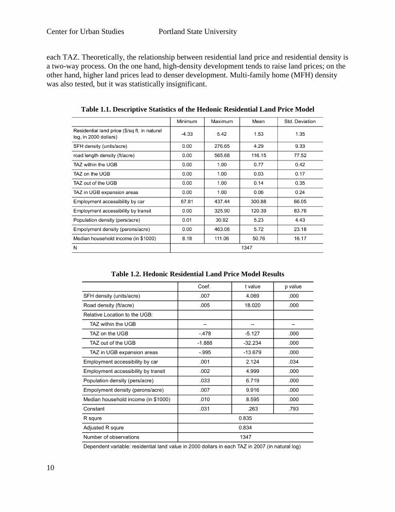
Model estimation results are shown in Table 1.2. As Table 1.2 indicates, the adjusted R-squared
is very high (0.84), suggesting that explanatory variables in the model can explain land price
very well. Specifically, land price rises with the increase of single-family home (SFH) density,
which is measured by the number of SFH units divided by the acres of land occupied by them in
Center for Urban Studies Portland State University
10
each TAZ. Theoretically, the relationship between residential land price and residential density is
a two-way process. On the one hand, high-density development tends to raise land prices; on the
other hand, higher land prices lead to denser development. Multi-family home (MFH) density
was also tested, but it was statistically insignificant.
Table 1.1. Descriptive Statistics of the Hedonic Residential Land Price Model
Table 1.2. Hedonic Residential Land Price Model Results
Center for Urban Studies Portland State University
11
Road density is used to represent the concentration of infrastructure in each TAZ, which has a
significant, positive effect on land price. The parameters of UGB variables are also consistent
with our expectation: land in UGB peripheral areas and land outside of the UGB tend to have
lower prices than land within the UGB. Model results show that locations with better auto and
transit accessibility to employment tend to have higher land prices, which also makes sense.
The results of socio-economic variables indicate that locations with higher population density,
employment density, and average household income tend to have higher land prices.
Commercial Land Price Model
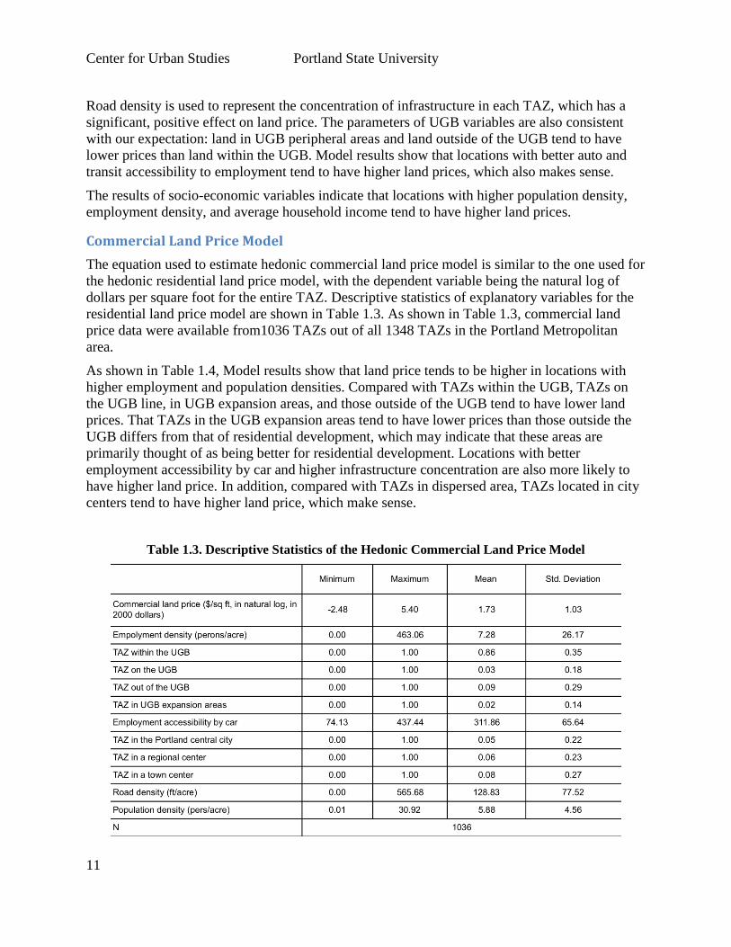
The equation used to estimate hedonic commercial land price model is similar to the one used for
the hedonic residential land price model, with the dependent variable being the natural log of
dollars per square foot for the entire TAZ. Descriptive statistics of explanatory variables for the
residential land price model are shown in Table 1.3. As shown in Table 1.3, commercial land
price data were available from1036 TAZs out of all 1348 TAZs in the Portland Metropolitan
area.
As shown in Table 1.4, Model results show that land price tends to be higher in locations with
higher employment and population densities. Compared with TAZs within the UGB, TAZs on
the UGB line, in UGB expansion areas, and those outside of the UGB tend to have lower land
prices. That TAZs in the UGB expansion areas tend to have lower prices than those outside the
UGB differs from that of residential development, which may indicate that these areas are
primarily thought of as being better for residential development. Locations with better
employment accessibility by car and higher infrastructure concentration are also more likely to
have higher land price. In addition, compared with TAZs in dispersed area, TAZs located in city
centers tend to have higher land price, which make sense.
Table 1.3. Descriptive Statistics of the Hedonic Commercial Land Price Model

Center for Urban Studies Portland State University
12
Table 1.4. Hedonic Commercial Land Price Model Results
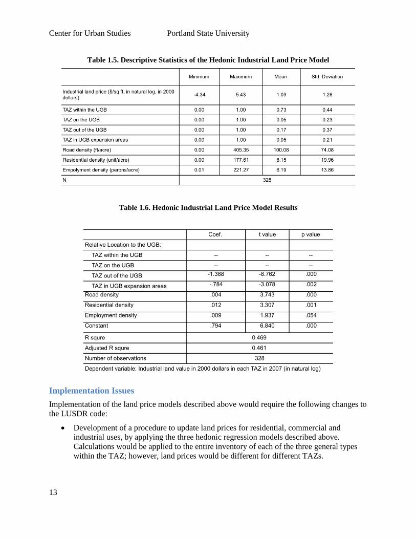
Industrial Land Price Model
The industrial land price model equation is also similar to the equations for residential and
commercial land price models; however, there are significantly fewer TAZs that have industrial
land. As Table 1.5, below, indicates, industrial land price data were only available from 328
TAZs out of all 1348 TAZs. Thus, the number of observations for the industrial land price model
is much smaller.
Many model specifications were tested. Table 1.6 shows the model with only significant
explanatory variables. The adjusted R-squared is smaller than those of the residential and
commercial models. As the table suggests, industrial land price tend to be higher in locations
with higher employment and residential density. Accessibility variables were not statistically
significant, possibly due to the fact that large industrial development tends to locate away from
population and commercial centers; however, locations with higher infrastructure concentration
are more likely to have higher industrial land prices. Model results also show that TAZs on the
UGB boundary are not significantly different from TAZs within the UGB in terms of industrial
land price. However, TAZs outside of the UGB and in UGB expansion areas tend to have lower
industrial land prices than TAZs within the UGB.
Center for Urban Studies Portland State University
13
Table 1.5. Descriptive Statistics of the Hedonic Industrial Land Price Model
Table 1.6. Hedonic Industrial Land Price Model Results
Implementation Issues
Implementation of the land price models described above would require the following changes to
the LUSDR code:
Development of a procedure to update land prices for residential, commercial and
industrial uses, by applying the three hedonic regression models described above.
Calculations would be applied to the entire inventory of each of the three general types
within the TAZ; however, land prices would be different for different TAZs.

Center for Urban Studies Portland State University
14
Given LUSDR’s extant order of operations, the households/population and employment
and accessibility calculations derived from the preceding modeling period would provide
inputs to each model calculation.
Additional variables to be created would be road density, which would ideally come from
an “all streets” network GIS file. This does not have to be routable and could come from
a TIGER line file, NAVTEK network, or similar sources.
Other variables to be created, using GIS, would be the status of each TAZ relative to the
urban growth boundary (within, on, in the expansion area, or outside).
Implementation of this method implies a fundamental change in the way in which LUSDR uses
land prices. Previously, a development cluster would have a bid price based on the type of
development and number of employees. If the proposed method were to be used, then the price
would be established as a supply attribute, and developers would choose whether to locate their
developments in a particular TAZ, based in part on the price of the land in that TAZ.
This has additional implications for how the development-cluster location choice modeling
works. It suggests a model that chooses a TAZ based on its attributes, from the perspective of the
developer, should be developed. Such multinomial choice models were developed under Task 5
(commercial development) and Task 11 (residential development). As may be seen under these
task descriptions, however, the resultant estimated models in both cases did not include land
price as an explanatory variable. This is because these models include many of the same
explanatory variables that were used to calculate land price, leading to severe multi-colinearity.
Moreover, to include land price in the model would in many cases lead to counter-intuitive
results where, all else being equal, higher priced land is more attractive.
Instead, it is recommended that land price be considered as a way of inducing redevelopment of
existing (under-utilized) land, which will lead to denser development as land prices rise. This
concept is discussed in greater detail under Task 12.

Center for Urban Studies Portland State University
15
2. Splitting Development Types
The impetus for a method to split development types in LUSDR was the mechanical problem
encountered in locating development clusters when space became a scarce commodity. As
mentioned above, maintaining development clusters may be viewed as more realistic because
development tends to be lumpy; however, it comes at a cost of computational problems. In
addition, Task 3, described below as a Land Fragmentation Procedure, is intended to make siting
developments even more difficult in zones that are more built out, because it tries to account for
the fact that available space is likely to be non-contiguous.
One solution to this problem is to allow for “densification,” which is a desirable property anyway
and relaxes LUSDR’s implicit assumption that all development clusters of a particular industry
type consume the same per-unit amount of space (housing units or employment units—jobs).
The question of densification is addressed in other tasks, as well, including the Task 1 Land Price
Model and Task 12 Development Degradation and Redevelopment.
Even with these density and redevelopment possibilities, however, there will likely remain
problems siting large development clusters. Mechanical solutions, such as simply dividing
unallocated clusters in half until they are eventually all sited would be an easy enough solution,
though it does not provide a particularly interesting research problem.
A more interesting research question asked by the study team is: “What are the statistical and
performance implications of forecasting the location of development in a clustered format,
compared with a less realistic “atomized” format, i.e., forecasting unit by unit?” To address this
question, the study team, led by Hongwei Dong, compared three methods for modeling and
forecasting residential development location choices. A detailed account of this experiment
was published in Transportation Research Record and is included as Appendix B to this
report.
Summary of Findings on Forecasting Methods
In this paper, we discuss three forecasting methods for developer project location choices, using
the developer as a decision making agent, which differs from the current version of LUSDR.
This was a top-down approach in which we generated a new housing supply each simulation
year, and then allocate them in space to TAZ, which compete with each other for development
where supply exists. Details of the basic approach may be found in Task 10, Housing Type
Choice.
In LUSDR’s current concept, the allocation of development units is a bottom-up approach,
representing the probability of each individual zone including a development of that particular
type. In addition, developments are allocated as an entire unit as they are in real life (e.g., a
subdivision with 100 housing units). This research found that it was very difficult to be accurate
in forecasting the locations of "lumpy" units like this. In this example, if you miss the mark,
which is the majority of the scenarios, you miss by 100 housing units in one shot. Even though it
is less realistic, you have less forecasting error if you just forecast the locations of individual
houses, one at a time.
Center for Urban Studies Portland State University
16
Using data from the Portland housing market, including Clark County, Washington, we
estimated and applied three new single-family housing location choice models. In the regional
housing market, a relatively small number of commercial developers account for the majority of
new housing with large projects; however, there are also several medium-sized developers, and
numerous small developers, who are typically private individuals who build their own homes.
Thus differentiating between developers and their project sizes could be an advantage.
Model 1 treated each housing unit as a separate location choice decision, effectively “atomizing”
developer projects, regardless of size. Model 2 assumed deterministic developer characteristics
and was based on the locating of the entire project as a single unit. Model 3 was also based on
the entire-project concepts, but used a latent class approach to probabilistically assign a
developer behavior type.
We found that all three models could successfully capture the basic spatial pattern of single-
family-home developments in the region. Although Models 2 and 3 were more sophisticated and
more theoretically appealing, they did not produce better forecast results than Model 1 because
of some practical issues, including the lack of developer information for forecast years, the small
sample size of large projects, the physics of forecasting a small number of large projects across a
large number of location alternatives, the need to sample large numbers of alternatives when
non-multinomial logit models were estimated, and the difficulty of using dummy variables in
latent class models. In this particular context, the simpler model specification proved to be both
easier to implement and more accurate. Models 2 and 3, however, were expected to perform
better when those practical issues are solved, at least partially, in further research.

Center for Urban Studies Portland State University
17
3. Land Fragmentation Procedure
In an effort to make development location choice more realistic in LUSDR, the study team, led
by Joshua Roll, developed a procedure to account for the amount of already developed land in a
TAZ when the program attempts to locate a development. The objective of this procedure is to
recognize that as a zone becomes more densely developed, fragmentation of land into multiple
parcels is likely to result in remaining vacant parcels that are smaller, not contiguous and
therefore not necessarily available for assembly to support large developments. Adopting either a
parcel-based system or a fine-resolution grid-based system would, in theory, provide the ability
to address this problem. Both of these options are very data-intensive, however, and would
require a large investment of time and resources for any implementing agency. Since ease of
implementation and simplicity are a guiding principle of LUSDR, the investigation focused on
other “pseudo-parcel-based” methods that would require fewer resources and achieve the same
general objective.
Currently, LUSDR uses a location choice model to determine the location of developments. This
process uses a number of relevant TAZ attributes such as slope, distance to the nearest freeway
interchange, traffic exposure, local employment accessibility, regional employment accessibility,
local household accessibility, and regional household accessibility, but neglects to consider the
density of a zone. The proposed method aims to reflect the amount of development already
occurring in the TAZ and thus act as a probabilistic estimate of vacant parcel size.
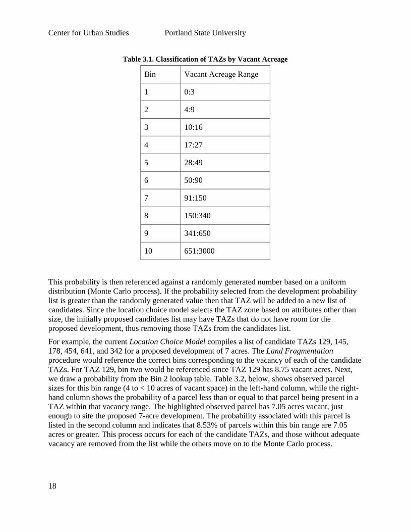
Data and Method
The recently developed Land Fragmentation procedure uses the parcel level data currently used
in the latest version of LUSDR for the Rogue Valley MPO (RVMPO). TAZs are classified into
one of ten bins based on the amount of total vacant acreage. The ranges of these bins were
selected by separating the approximately 10,000 parcels into equal-size bins with around 1,000
parcels per bin (see Table 3.1 below for bin ranges). These ranges were determined based on a
non-linear relationship between the amount of vacant acreage in a TAZ and the presence of
large, vacant parcels.
The procedure follows directly after the outcome of the current location choice procedure in
which LUSDR has chosen a number of TAZs suitable for the proposed development. Based on
the amount of vacant acres in the chosen TAZ, one of the ten bin ranges is assigned. Each bin
represents a different cumulative distribution function, which was derived from the size of
observed parcels for TAZs within a certain range of observed vacancy, as shown in Table 3.1.
Given a proposed development of a certain size, the Land Fragmentation procedure then
generates the probability that a vacant parcel equal to or larger than the proposed development
will be present in the TAZ. The logic of this approach is to represent the fragmentation of land
that occurs through development, giving a greater probability to smaller developments, while
larger developments have lower probabilities of being located. The non-linear relationship
between the vacant parcel sizes and total vacant acreage is such that densely developed TAZs
have relatively few large parcels.
Center for Urban Studies Portland State University
18
Table 3.1. Classification of TAZs by Vacant Acreage
Bin Vacant Acreage Range
1 0:3
2 4:9
3 10:16
4 17:27
5 28:49
6 50:90
7 91:150
8 150:340
9 341:650
10 651:3000
This probability is then referenced against a randomly generated number based on a uniform
distribution (Monte Carlo process). If the probability selected from the development probability
list is greater than the randomly generated value then that TAZ will be added to a new list of
candidates. Since the location choice model selects the TAZ zone based on attributes other than
size, the initially proposed candidates list may have TAZs that do not have room for the
proposed development, thus removing those TAZs from the candidates list.
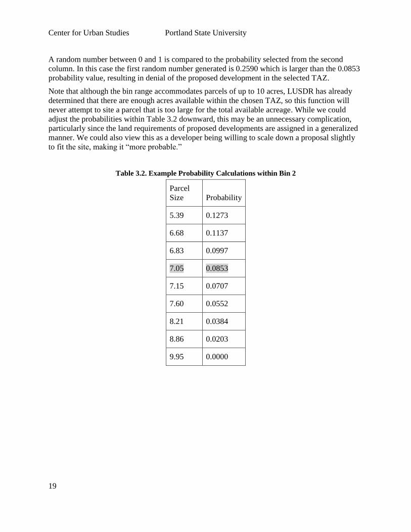
For example, the current Location Choice Model compiles a list of candidate TAZs 129, 145,
178, 454, 641, and 342 for a proposed development of 7 acres. The Land Fragmentation
procedure would reference the correct bins corresponding to the vacancy of each of the candidate
TAZs. For TAZ 129, bin two would be referenced since TAZ 129 has 8.75 vacant acres. Next,
we draw a probability from the Bin 2 lookup table. Table 3.2, below, shows observed parcel
sizes for this bin range (4 to < 10 acres of vacant space) in the left-hand column, while the right-
hand column shows the probability of a parcel less than or equal to that parcel being present in a
TAZ within that vacancy range. The highlighted observed parcel has 7.05 acres vacant, just
enough to site the proposed 7-acre development. The probability associated with this parcel is
listed in the second column and indicates that 8.53% of parcels within this bin range are 7.05
acres or greater. This process occurs for each of the candidate TAZs, and those without adequate
vacancy are removed from the list while the others move on to the Monte Carlo process.
Center for Urban Studies Portland State University
19
A random number between 0 and 1 is compared to the probability selected from the second
column. In this case the first random number generated is 0.2590 which is larger than the 0.0853
probability value, resulting in denial of the proposed development in the selected TAZ.
Note that although the bin range accommodates parcels of up to 10 acres, LUSDR has already
determined that there are enough acres available within the chosen TAZ, so this function will
never attempt to site a parcel that is too large for the total available acreage. While we could
adjust the probabilities within Table 3.2 downward, this may be an unnecessary complication,
particularly since the land requirements of proposed developments are assigned in a generalized
manner. We could also view this as a developer being willing to scale down a proposal slightly
to fit the site, making it “more probable.”
Table 3.2. Example Probability Calculations within Bin 2
Parcel
Size Probability
5.39 0.1273
6.68 0.1137
6.83 0.0997
7.05 0.0853
7.15 0.0707
7.60 0.0552
8.21 0.0384
8.86 0.0203
9.95 0.0000
Center for Urban Studies Portland State University
20
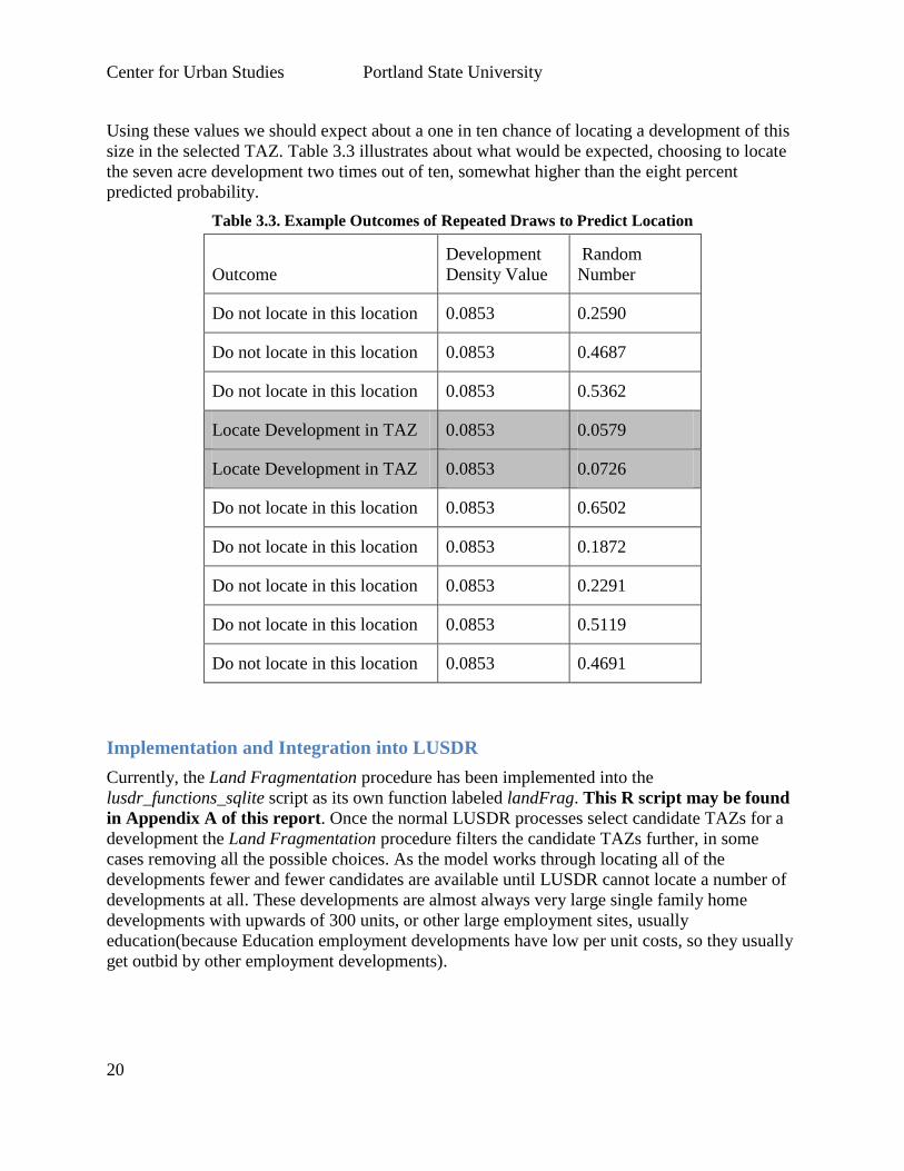
Using these values we should expect about a one in ten chance of locating a development of this
size in the selected TAZ. Table 3.3 illustrates about what would be expected, choosing to locate
the seven acre development two times out of ten, somewhat higher than the eight percent
predicted probability.
Table 3.3. Example Outcomes of Repeated Draws to Predict Location
Outcome
Development
Density Value
Random
Number
Do not locate in this location 0.0853 0.2590
Do not locate in this location 0.0853 0.4687
Do not locate in this location 0.0853 0.5362
Locate Development in TAZ 0.0853 0.0579
Locate Development in TAZ 0.0853 0.0726
Do not locate in this location 0.0853 0.6502
Do not locate in this location 0.0853 0.1872
Do not locate in this location 0.0853 0.2291
Do not locate in this location 0.0853 0.5119
Do not locate in this location 0.0853 0.4691
Implementation and Integration into LUSDR
Currently, the Land Fragmentation procedure has been implemented into the
lusdr_functions_sqlite script as its own function labeled landFrag. This R script may be found
in Appendix A of this report. Once the normal LUSDR processes select candidate TAZs for a
development the Land Fragmentation procedure filters the candidate TAZs further, in some
cases removing all the possible choices. As the model works through locating all of the
developments fewer and fewer candidates are available until LUSDR cannot locate a number of
developments at all. These developments are almost always very large single family home
developments with upwards of 300 units, or other large employment sites, usually
education(because Education employment developments have low per unit costs, so they usually
get outbid by other employment developments).
Center for Urban Studies Portland State University
21
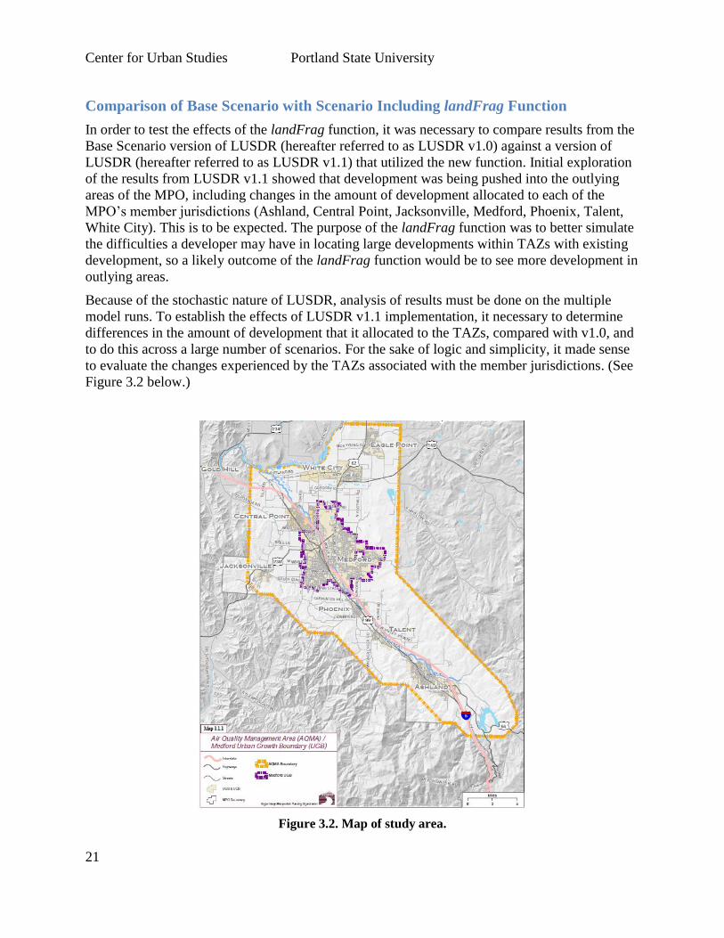
Comparison of Base Scenario with Scenario Including landFrag Function
In order to test the effects of the landFrag function, it was necessary to compare results from the
Base Scenario version of LUSDR (hereafter referred to as LUSDR v1.0) against a version of
LUSDR (hereafter referred to as LUSDR v1.1) that utilized the new function. Initial exploration
of the results from LUSDR v1.1 showed that development was being pushed into the outlying
areas of the MPO, including changes in the amount of development allocated to each of the
MPO’s member jurisdictions (Ashland, Central Point, Jacksonville, Medford, Phoenix, Talent,
White City). This is to be expected. The purpose of the landFrag function was to better simulate
the difficulties a developer may have in locating large developments within TAZs with existing
development, so a likely outcome of the landFrag function would be to see more development in
outlying areas.
Because of the stochastic nature of LUSDR, analysis of results must be done on the multiple
model runs. To establish the effects of LUSDR v1.1 implementation, it necessary to determine
differences in the amount of development that it allocated to the TAZs, compared with v1.0, and
to do this across a large number of scenarios. For the sake of logic and simplicity, it made sense
to evaluate the changes experienced by the TAZs associated with the member jurisdictions. (See
Figure 3.2 below.)
Figure 3.2. Map of study area.
Center for Urban Studies Portland State University
22
Because the landFrag function imposes additional constraints on the ability of LUSDR to site
new developments, a number of developments were unable to locate anywhere within the area.
These developments are usually huge single-family developments of 300-plus units or
educational employment sites, the latter possessing a very low per unit price, allowing it to be
outbid when it comes into competition with other employment developments.
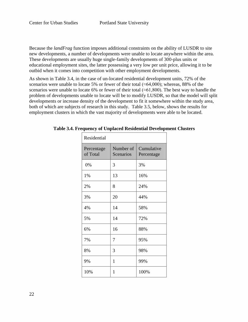
As shown in Table 3.4, in the case of un-located residential development units, 72% of the
scenarios were unable to locate 5% or fewer of their total (≈64,000); whereas, 88% of the
scenarios were unable to locate 6% or fewer of their total (≈61,800). The best way to handle the
problem of developments unable to locate will be to modify LUSDR, so that the model will split
developments or increase density of the development to fit it somewhere within the study area,
both of which are subjects of research in this study. Table 3.5, below, shows the results for
employment clusters in which the vast majority of developments were able to be located.
Table 3.4. Frequency of Unplaced Residential Development Clusters
Residential
Percentage
of Total
Number of
Scenarios
Cumulative
Percentage
0% 3 3%
1% 13 16%
2% 8 24%
3% 20 44%
4% 14 58%
5% 14 72%
6% 16 88%
7% 7 95%
8% 3 98%
9% 1 99%
10% 1 100%

Center for Urban Studies Portland State University
23
Table 3.5. Frequency of Unplaced Employment Development Clusters
Employment
Percentage of
Total
Number of
Scenarios
Cumulative
Percentage
0% 44 44%
1% 44 88%
2% 9 97%
3% 2 99%
4% 1 100%
The first set of tests was done comparing LUSDR v1.0 outputs against itself. Because of the
variability of LUSDR’s outputs due to stochasticity, it was important to demonstrate that the
development distributions of each member jurisdictions were consistent across runs of the same
model before demonstrating differences from the new model, LUSDR v1.1. For all tests, two sets
of 100 runs were analyzed.
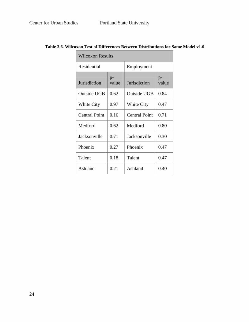
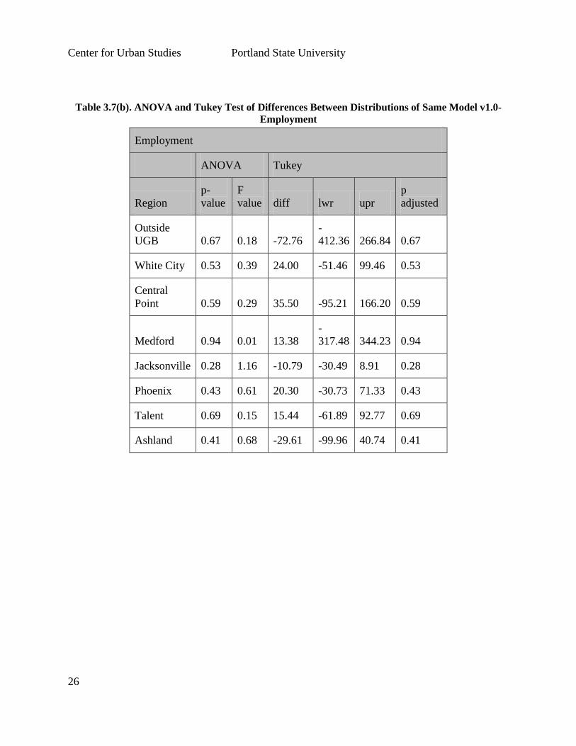
A set of Wilcoxon tests were used to see if any difference existed between scenario runs from the
results of LUSDR v1.0. Each jurisdiction’s TAZs development distributions were compared
against each other with results, showing no significant difference (See Table 3.6). Tests
analyzing differences using one-way ANOVA and Tukey tests also indicate no difference in the
two distributions. (See Table 3.7(a) & (b)).
Center for Urban Studies Portland State University
24
Table 3.6. Wilcoxon Test of Differences Between Distributions for Same Model v1.0
Wilcoxon Results
Residential Employment
Jurisdiction
p-
value Jurisdiction
p-
value
Outside UGB 0.62 Outside UGB 0.84
White City 0.97 White City 0.47
Central Point 0.16 Central Point 0.71
Medford 0.62 Medford 0.80
Jacksonville 0.71 Jacksonville 0.30
Phoenix 0.27 Phoenix 0.47
Talent 0.18 Talent 0.47
Ashland 0.21 Ashland 0.40

Center for Urban Studies Portland State University
25
Table 3.7 (a) ANOVA and Tukey Test of Differences Between Distributions of Same Model v1.0-
Residential
Residential
ANOVA Tukey
Region
p-
value
F
value diff lwr upr
p
adjusted
Outside
UGB 0.45 0.57 102.84
-
165.61 371.29 0.45
White City 0.90 0.02 7.16
-
105.83 120.15 0.90
Central
Point 0.16 2.01 -69.66
-
166.15 26.84 0.16
Medford 0.84 0.04 26.71
-
240.08 293.50 0.84
Jacksonville 0.50 0.45 -9.17 -36.12 17.78 0.50
Phoenix 0.52 0.41 9.81 -20.41 40.02 0.52
Talent 0.18 1.82 -26.75 -65.69 12.19 0.18
Ashland 0.13 2.30 -49.95
-
114.63 14.73 0.13
Center for Urban Studies Portland State University
26
Table 3.7(b). ANOVA and Tukey Test of Differences Between Distributions of Same Model v1.0-
Employment
Employment
ANOVA Tukey
Region
p-
value
F
value diff lwr upr
p
adjusted
Outside
UGB 0.67 0.18 -72.76
-
412.36 266.84 0.67
White City 0.53 0.39 24.00 -51.46 99.46 0.53
Central
Point 0.59 0.29 35.50 -95.21 166.20 0.59
Medford 0.94 0.01 13.38
-
317.48 344.23 0.94
Jacksonville 0.28 1.16 -10.79 -30.49 8.91 0.28
Phoenix 0.43 0.61 20.30 -30.73 71.33 0.43
Talent 0.69 0.15 15.44 -61.89 92.77 0.69
Ashland 0.41 0.68 -29.61 -99.96 40.74 0.41
Center for Urban Studies Portland State University
27
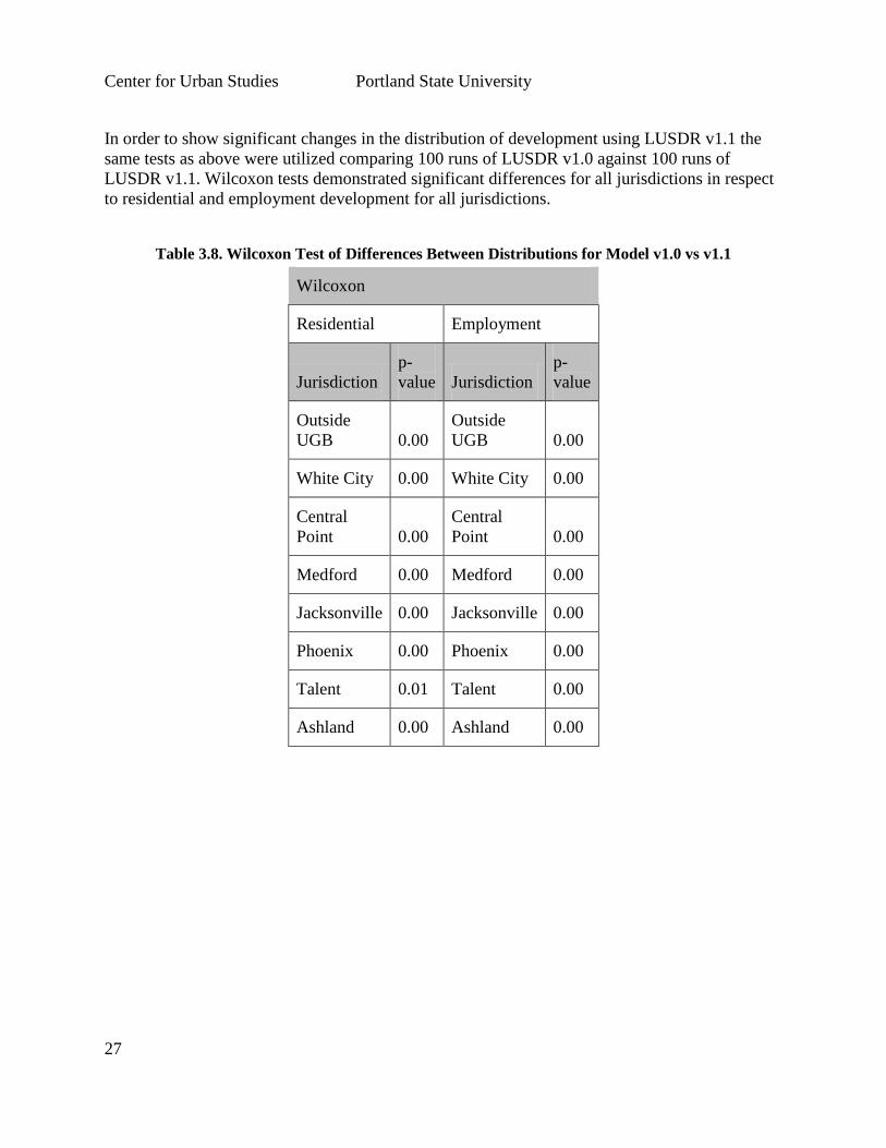
In order to show significant changes in the distribution of development using LUSDR v1.1 the
same tests as above were utilized comparing 100 runs of LUSDR v1.0 against 100 runs of
LUSDR v1.1. Wilcoxon tests demonstrated significant differences for all jurisdictions in respect
to residential and employment development for all jurisdictions.
Table 3.8. Wilcoxon Test of Differences Between Distributions for Model v1.0 vs v1.1
Wilcoxon
Residential Employment
Jurisdiction
p-
value Jurisdiction
p-
value
Outside
UGB 0.00
Outside
UGB 0.00
White City 0.00 White City 0.00
Central
Point 0.00
Central
Point 0.00
Medford 0.00 Medford 0.00
Jacksonville 0.00 Jacksonville 0.00
Phoenix 0.00 Phoenix 0.00
Talent 0.01 Talent 0.00
Ashland 0.00 Ashland 0.00
Center for Urban Studies Portland State University
28
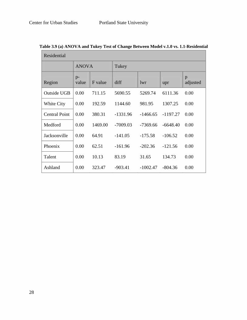
Table 3.9 (a) ANOVA and Tukey Test of Change Between Model v.1.0 vs. 1.1-Residential
Residential
ANOVA Tukey
Region
p-
value F value diff lwr upr
p
adjusted
Outside UGB 0.00 711.15 5690.55 5269.74 6111.36 0.00
White City 0.00 192.59 1144.60 981.95 1307.25 0.00
Central Point 0.00 380.31 -1331.96 -1466.65 -1197.27 0.00
Medford 0.00 1469.00 -7009.03 -7369.66 -6648.40 0.00
Jacksonville 0.00 64.91 -141.05 -175.58 -106.52 0.00
Phoenix 0.00 62.51 -161.96 -202.36 -121.56 0.00
Talent 0.00 10.13 83.19 31.65 134.73 0.00
Ashland 0.00 323.47 -903.41 -1002.47 -804.36 0.00
Center for Urban Studies Portland State University
29
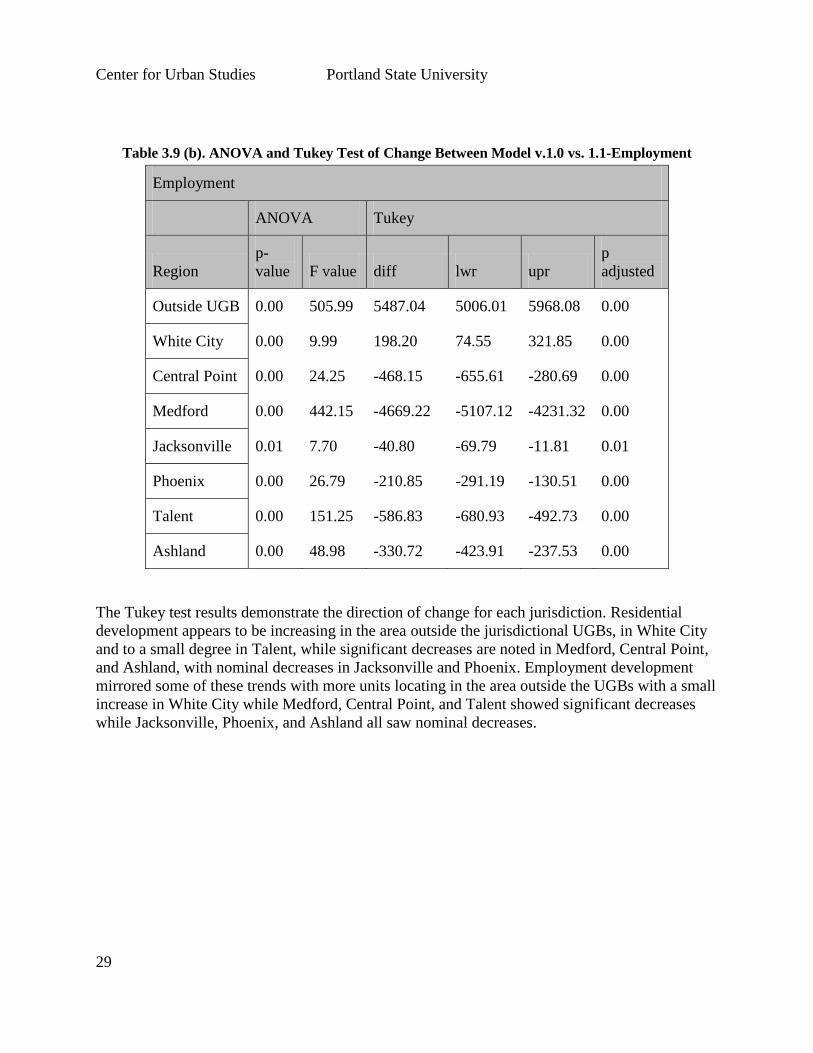
Table 3.9 (b). ANOVA and Tukey Test of Change Between Model v.1.0 vs. 1.1-Employment
Employment
ANOVA Tukey
Region
p-
value F value diff lwr upr
p
adjusted
Outside UGB 0.00 505.99 5487.04 5006.01 5968.08 0.00
White City 0.00 9.99 198.20 74.55 321.85 0.00
Central Point 0.00 24.25 -468.15 -655.61 -280.69 0.00
Medford 0.00 442.15 -4669.22 -5107.12 -4231.32 0.00
Jacksonville 0.01 7.70 -40.80 -69.79 -11.81 0.01
Phoenix 0.00 26.79 -210.85 -291.19 -130.51 0.00
Talent 0.00 151.25 -586.83 -680.93 -492.73 0.00
Ashland 0.00 48.98 -330.72 -423.91 -237.53 0.00
The Tukey test results demonstrate the direction of change for each jurisdiction. Residential
development appears to be increasing in the area outside the jurisdictional UGBs, in White City
and to a small degree in Talent, while significant decreases are noted in Medford, Central Point,
and Ashland, with nominal decreases in Jacksonville and Phoenix. Employment development
mirrored some of these trends with more units locating in the area outside the UGBs with a small
increase in White City while Medford, Central Point, and Talent showed significant decreases
while Jacksonville, Phoenix, and Ashland all saw nominal decreases.

Center for Urban Studies Portland State University
30
4. Fixed Development Types
The objective of this task was to develop a module to account for land uses that are better
modeled as fixed development types, independent of market control, such as public facilities,
schools, hospitals, sports stadiums, tourist attractions and similar uses. This feature could also be
used to model very large market-based developments that have been proposed and are the subject
of an impact analysis. In these cases, it may be assumed that the proposed development will
happen, and the analysis makes that explicit in modeling impacts not only on the transportation
system, but also on land development elsewhere, possibly in response to the proposed
development.
Proposed Approach
The recommended approach is a fairly straightforward creation of a table to hold the fixed
development records and their attributes. This is similar to what is done in the land use modeling
package, UrbanSim. At the beginning of each simulation, LUSDR would automatically create
the developments listed in the table, using specified locations and forecast year of opening. In
many cases, a development may be phased in over several years. If this phasing plan is known or
assumed, then each phase should be entered into the table as a separate record. The data used to
populate the fields in the table should come from development master plans or other source of
reliable local knowledge, with additional assumptions as to the likely occupancy rate of the
development, both at project opening and at its long-term occupancy rate (e.g., after 10 years).
Depending on the nature of the development—commercial, residential, mixed use, or public—
there will be space created to accommodate regional employment and, potentially, residences.
Algorithmically, the employment and households should be placed at these fixed development
locations prior to allocating households and employment clusters among the general land use
types. This may be as simple as identifying upfront the number and industry types of
employment that are likely to occupy the proposed development and removing those from the
pool of new employment to allocated through LUSDR’s main market-based employment cluster
procedure. Similarly, the type of housing to be made available through the proposed
development should be made explicit in the table data—single-family vs. multi-family.
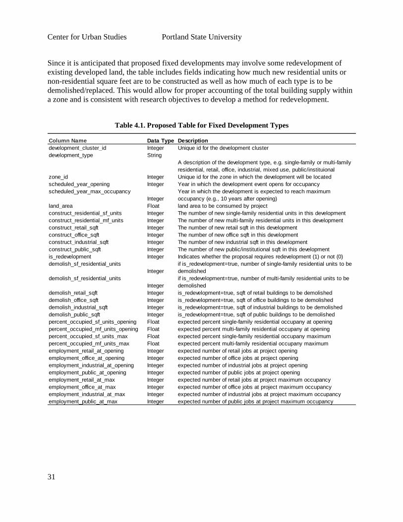
An example of a data format for this table is shown below in Table 4.1. This table includes fields
identifying the development cluster itself, and the zone (TAZ) in which it would be placed. The
amount of land to be consumed by the project is one key entry, as it takes this land out of the
available supply. In terms of timing, the table identifies the year at which the fixed development
would be expected to open and the year at which it would be expected to achieve its long-term
occupancy rate.
This example includes two types of residential development—single- and multi-family—as
corresponding to the types used in LUSDR currently. It also includes four types of non-
residential development—retail, office, industrial and public/institutional. These non-residential
descriptors refer to the type of building in which employment is likely to occupy. This further
assumes that a new development type will be created for LUSDR to accommodate public and
institutional employment.
Center for Urban Studies Portland State University
31
Since it is anticipated that proposed fixed developments may involve some redevelopment of
existing developed land, the table includes fields indicating how much new residential units or
non-residential square feet are to be constructed as well as how much of each type is to be
demolished/replaced. This would allow for proper accounting of the total building supply within
a zone and is consistent with research objectives to develop a method for redevelopment.
Table 4.1. Proposed Table for Fixed Development Types
Column Name Data Type Description
development_cluster_id Integer Unique id for the development cluster
development_type String
A description of the development type, e.g. single-family or multi-family
residential, retail, office, industrial, mixed use, public/instituional
zone_id Integer Unique id for the zone in which the development will be located
scheduled_year_opening Integer Year in which the development event opens for occupancy
scheduled_year_max_occupancy
Integer
Year in which the development is expected to reach maximum
occupancy (e.g., 10 years after opening)
land_area Float land area to be consumed by project
construct_residential_sf_units Integer The number of new single-family residential units in this development
construct_residential_mf_units Integer The number of new multi-family residential units in this development
construct_retail_sqft Integer The number of new retail sqft in this development
construct_office_sqft Integer The number of new office sqft in this development
construct_industrial_sqft Integer The number of new industrial sqft in this development
construct_public_sqft Integer The number of new public/institutional sqft in this development
is_redevelopment Integer Indicates whether the proposal requires redevelopment (1) or not (0)
demolish_sf_residential_units
Integer
if is_redevelopment=true, number of single-family residential units to be
demolished
demolish_sf_residential_units
Integer
if is_redevelopment=true, number of multi-family residential units to be
demolished
demolish_retail_sqft Integer is_redevelopment=true, sqft of retail buildings to be demolished
demolish_office_sqft Integer is_redevelopment=true, sqft of office buildings to be demolished
demolish_industrial_sqft Integer is_redevelopment=true, sqft of industrial buildings to be demolished
demolish_public_sqft Integer is_redevelopment=true, sqft of public buildings to be demolished
percent_occupied_sf_units_opening Float expected percent single-family residential occupany at opening
percent_occupied_mf_units_opening Float expected percent multi-family residential occupany at opening
percent_occupied_sf_units_max Float expected percent single-family residential occupany maximum
percent_occupied_mf_units_max Float expected percent multi-family residential occupany maximum
employment_retail_at_opening Integer expected number of retail jobs at project opening
employment_office_at_opening Integer expected number of office jobs at project opening
employment_industrial_at_opening Integer expected number of industrial jobs at project opening
employment_public_at_opening Integer expected number of public jobs at project opening
employment_retail_at_max Integer expected number of retail jobs at project maximum occupancy
employment_office_at_max Integer expected number of office jobs at project maximum occupancy
employment_industrial_at_max Integer expected number of industrial jobs at project maximum occupancy
employment_public_at_max Integer expected number of public jobs at project maximum occupancy
Center for Urban Studies Portland State University
32
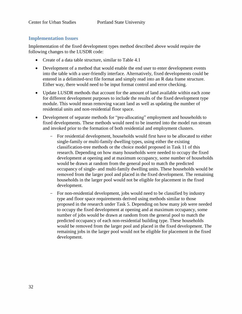
Implementation Issues
Implementation of the fixed development types method described above would require the
following changes to the LUSDR code:
Create of a data table structure, similar to Table 4.1
Development of a method that would enable the end user to enter development events
into the table with a user-friendly interface. Alternatively, fixed developments could be
entered in a delimited-text file format and simply read into an R data frame structure.
Either way, there would need to be input format control and error checking.
Update LUSDR methods that account for the amount of land available within each zone
for different development purposes to include the results of the fixed development type
module. This would mean removing vacant land as well as updating the number of
residential units and non-residential floor space.
Development of separate methods for “pre-allocating” employment and households to
fixed developments. These methods would need to be inserted into the model run stream
and invoked prior to the formation of both residential and employment clusters.
For residential development, households would first have to be allocated to either
single-family or multi-family dwelling types, using either the existing
classification-tree methods or the choice model proposed in Task 11 of this
research. Depending on how many households were needed to occupy the fixed
development at opening and at maximum occupancy, some number of households
would be drawn at random from the general pool to match the predicted
occupancy of single- and multi-family dwelling units. These households would be
removed from the larger pool and placed in the fixed development. The remaining
households in the larger pool would not be eligible for placement in the fixed
development.
For non-residential development, jobs would need to be classified by industry
type and floor space requirements derived using methods similar to those
proposed in the research under Task 5. Depending on how many job were needed
to occupy the fixed development at opening and at maximum occupancy, some
number of jobs would be drawn at random from the general pool to match the
predicted occupancy of each non-residential building type. These households
would be removed from the larger pool and placed in the fixed development. The
remaining jobs in the larger pool would not be eligible for placement in the fixed
development.

Center for Urban Studies Portland State University
33
5. Endogenously Determined Employment Mix
The objective of this task was to develop a method by which the spatial distribution of
employment of different types would be determined endogenously. In the original form, LUSDR
determines the total number of jobs in the region by the number of workers predicted in
households and adjusts this number based on the historical ratio of workers to jobs in the region.
Jobs are then allocated to industry types based on an assumed historical or predicted distribution
by 2-digit NAICS code; jobs by industry are assigned to firms based on historical distributions of
firm size; and firms are assigned to development clusters based on historical distributions of
cluster sizes. The placement of development clusters in zones is based on a calculation of the
probability of a particular zone attracting an employment development, based on attraction
factors, including plan compatibility and space availability. These probabilities are used as
weights, and employment clusters are located by random draws of zones, proportional to these
weights.
LUSDR’s current approach to predicting the probability that a specific type of development will
be located in a TAZ is the reverse of how location choices are usually predicted in land use
models. It is more common in land use modeling to model the probability of choosing a site for
the location of a specific development. The main idea is that the developer is choosing the
location of the development, rather than the zone “choosing” to be developed. This would be a
more theoretically acceptable treatment and allows for consideration of developer characteristics
and preferences when formulating models. In the remainder of this section we describe a model
developed for this purpose.
Figure 5.1 indicates the commercial real estate model designed for LUSDR, which is a 3-step
model. In the first two steps, the total amount of new employment is predicted and decomposed
into employment clusters.
Through observed floor space per employee ratio by industry sectors, employment clusters are
transformed into new commercial development clusters. In the third step, commercial
development clusters are located into zones by the commercial cluster location choice model.
Since the first two models already exist in LUSDR model, in this report, we present the location
choice model only.

Center for Urban Studies Portland State University
34
Figure 5.1. Commercial real estate model
Commercial Development Location Choice Model
Data
The data used for this estimation work was derived from the 2007 Portland MetroRLIS data set.
It was chosen because it offers a large number of samples and a diverse set of urban
environments and densities.
Methodology
Similar to the residential development location choice model, the commercial development
cluster location choice location models are derived as follows. Each developer faces a choice
among alternative locations. The developer obtains a certain level of utility from each
alternative location , and the utility is composed of two parts, the systematic portion and the
error :
For each alternative location , there is a set of alternative specific location attributes .
Assuming that the error in utility function is identically and independently distributed (IID)
Center for Urban Studies Portland State University
35
across alternatives and to follow a Gumbel distribution, the choice probability for location
alternative is:
( ) ( )
∑ ( )
where denotes the parameters for each location attribute. Discrete choice models developed
under these assumptions are called Multinomial logit (MNL) models.
Again, since it was neither computationally feasible nor theoretically realistic to assume that
developers would consider all the TAZs as alternatives in the choice set for each project, we used
a pure random sample of 19 alternative TAZs, plus the chosen TAZ as the choice set for each
developer. Alternatives were sampled without replacement and without any type of importance
sampling or stratification.
Input Data and Model Estimation
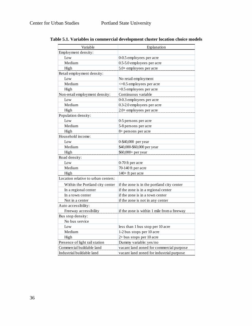
Table 5.1 explains variables used to predict the location choice of commercial development
clusters. The final set of estimated parameters may be seen in Table 5.2, which includes
estimates for one general model, and three market segments that were grouped based on
compatibility:
1. General model that could be used for all commercial development clusters;
2. Sales/customer-oriented building clusters (retail, wholesale, dining, and personal
care);
3. Office-oriented (professional services, banks, research and development); and
4. Other/industrial employment types (warehousing, manufacturing, public utilities,
agriculture and construction).
The estimation results show that developers will choose to locate commercial developments in
zones that already have a high density of commercial development, with a preference for the
same type of development. Since the spatial unit of analysis is the TAZ, this is consistent with
the notion that area zoning and comprehensive plans support these types of development. In
addition, the Office and Other categories tend to locate away from concentrations of residential
development. This can be further differentiated by a zone’s median household income range, in
which sales-oriented businesses are significantly more likely to locate near lower- income
households and significantly less likely to locate near higher income households. The
Other/industrial category developments are also significantly more likely to locate near lower
income households.
Both Sales and Office building types were significantly more likely to choose locations within
one mile of a freeway, or near regional and town centers. Office developments were more likely
to locate in a CBD. Interestingly, bus stop density had a significant negative impact on the
location choices for Sales and Other/industrial developments, whereas the presence of a light rail
station had a significant positive impact on the location choices of Sales and Office
developments.
Center for Urban Studies Portland State University
36
Table 5.1. Variables in commercial development cluster location choice models
Variable Explanation
Employment density:
Low 0-0.5 employees per acre
Medium 0.5-5.0 employees per acre
High 5.0+ employees per acre
Retail employment density:
Low No retail employment
Medium <=0.5 employees per acre
High >0.5 employees per acre
Non-retail employment density: Continuous variable
Low 0-0.3 employees per acre
Medium 0.3-2.0 employees per acre
High 2.0+ employees per acre
Population density:
Low 0-5 persons per acre
Medium 5-8 persons per acre
High 8+ persons per acre
Household income:
Low 0-$40,000 per year
Medium $40,000-$60,000 per year
High $60,000+ per year
Road density:
Low 0-70 ft per acre
Medium 70-140 ft per acre
High 140+ ft per acre
Location relative to urban centers:
Within the Portland city center if the zone is in the portland city center
In a regional center if the zone is in a regional center
In a town center if the zone is in a town center
Not in a center if the zone is not in any center
Auto accessibility:
Freeway accessibility if the zone is within 1 mile from a freeway
Bus stop density:
No bus service
Low less than 1 bus stop per 10 acre
Medium 1-2 bus stops per 10 acre
High 2+ bus stops per 10 acre
Presence of light rail station Dummy variable: yes/no
Commercial buildable land vacant land zoned for commercial purpose
Industrial buildable land vacant land zoned for industrial purpose
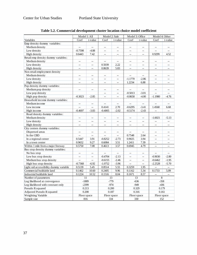
Center for Urban Studies Portland State University
37
Table 5.2. Commercial development cluster location choice model coefficient
Variables Coef t-value Coef t-value Coef t-value Coef t-value
Emp density dummy variables:
Medium density -- -- -- -- -- -- -- --
Low density -0.7598 -4.88 -- -- -- -- -- --
High density 0.6443 7.42 -- -- -- -- 0.9299 4.52
Retail emp density dummy variables:
Medium density -- -- -- -- -- -- -- --
Low density -- -- 0.5039 2.22 -- -- -- --
High density -- -- 0.8639 5.83 -- -- -- --
Non-retail employment density
Medium density -- -- -- -- -- -- -- --
Low density -- -- -- -- -1.1770 -2.86 -- --
High density -- -- -- -- 1.2234 6.88 -- --
Pop density dummy variables:
Medium pop density -- -- -- -- -- -- -- --
Low pop density -- -- -0.5013 -3.01 -- --
High pop density -0.3023 -2.85 -- -- -0.8658 -4.00 -1.1980 -4.76
Household income dummy variables:
Medium income -- -- -- -- -- -- -- --
Low income -- -- 0.4141 2.70 -0.6295 -3.41 1.4568 6.68
High income -0.4697 -3.83 -0.4005 -2.02 -0.5174 -2.43 -- --
Road density dummy variables:
Medium density -- -- -- -- -- -- -1.6021 -5.13
Low density -- -- -- -- -- -- -- --
High density -- -- -- -- -- -- -- --
City centers dummy variables:
Dispersed areas -- -- -- -- -- -- -- --
In the CBD -- -- -- -- 0.7548 2.64 -- --
In a regional center 0.5447 3.91 -0.8252 -2.73 0.9025 3.94 -- --
In a town center 0.9652 9.27 0.6084 3.51 1.2411 7.39 -- --
Within 1 mile from a major freeway 0.5750 7.08 0.4613 3.57 0.6945 4.79 -- --
Bus stop density dummy variables:
No bus stop -- -- -- -- -- -- -- --
Low bus stop density -- -- -0.4704 -2.13 -- -- -0.9030 -2.80
Medium bus stop density -- -- -0.6155 -2.46 -- -- -0.6462 -1.95
High bus stop density -0.7368 -6.92 -1.0752 -3.96 -- -- -2.2528 -5.70
Light rail accessibility dummy variable 0.5139 5.45 0.8514 5.55 0.3259 1.95 -- --
Commercial buildable land 0.1462 10.60 0.2405 9.96 0.1162 5.34 0.1733 5.09
Industrial buildable land 0.1224 10.52 0.1516 8.04 0.1671 8.57 -- --
Number of parameters
Log likelihood at convergence
Log likelihood with constant only
Pseudo R squared
Adjusted Pseudo R squared
Weighting Variable
Sample size
Floor space
816 334 330
Model 4: Other
152
8
-436
-358
0.179
0.1610.208 0.187 0.316
Floor space Floor space Floor space
-2399 -974 -949
0.213 0.200 0.329
11 13 13
-1889 -779 -636
Model 1: All Model 2: Sale Model 3: Office

Center for Urban Studies Portland State University
38
Implementation Issues
Implementation of the proposed method would require the following changes to the LUSDR
program:
Development of model inputs, such as road density, distance to freeways, bus stop
density, and presence of a light rail station. These need to be stored in the R data frame as
attributes of each TAZ.
A method would need to be added to the R code to implement the multinomial choice
model, applying Monte Carlo draws to pick an outcome, for either the one “general”
model types, or the three separate market segments (recommended).
While sampling of zone alternatives was used for model estimation, it is more
theoretically correct to use the full set of available zones as choice alternatives
when applying these models in the simulation. This can be done efficiently in R
by calculating utilities and probabilities in arrays, using linear algebra.

Center for Urban Studies Portland State University
39
6. Evaluation of Transferability
The strategy for evaluating the transferability of LUSDR to another modeling region was to port
the RVMPO (Medford) model to the Mid-Willamette Council of Governments’ Salem-Kaiser
Transportation Study (SKATS). The actual work of developing the model for the SKATS region
was performed by Mike Jaffe of SKATS, with some help from Brian Gregor of ODOT-TPAU.
The goals of the evaluation were relatively broad:
To identify any barriers to implementation, such data or program code that was specific
to the original RVMPO development and therefore needed to be generalized;
To test the performance of LUSDR on a regional modeling case study and assess the
model outputs for reasonableness; and
To identify elements of LUSDR that should be improved to support transferability.
Development and Testing Activities
As reported by Mike Jaffe (2009), he and the other SKATS staff involved in this effort:
Carefully read and re-read the documentation provided to them by ODOT-TPAU in an
effort to better understand how LUSDR is intended to work;
Developed data inputs to LUSDR that were specific to the Salem-Kaiser region;
Worked through unanticipated bugs in the code or data input formats;
Ran LUSDR and examined outputs across single and multiple scenarios and model
periods; and
Reviewed the model data and code to resolve additional bugs in the code and the data;
and
Asked questions to attempt to understand why the model produced the results that it did.
The following adjustments were made to LUSDR model components to fit the Salem-Kaiser
region:
Using local Census and PUMS data as inputs to the Household Model R-data file;
Grouping Salem’s detailed employment data (ES-202) to LUSDR’s employment
categories and updating the Employment Model R-data file;
Assembling the land use inventory data for the base year;
Generating the travel time skim data and “traffic exposure” measures (a proxy for traffic
flow, defined as the number of OD shortest paths in the vicinity of each TAZ);
Adding government employment to plan development-employment compatibility lookup
table; and
Specifying planning and analysis districts as aggregates of TAZs.

Center for Urban Studies Portland State University
40
General Findings
The general findings of the SKATS analysis team, as reported in 2009, were the following:
Parts of the code were specific to Rogue Valley MPO model. These included definitions
of households and employment groupings, as well as hardcoding file names and paths.
It was somewhat difficult to trace source of errors using R’s debug and tracing functions.
When LUSDR was unable to place a development cluster, it would often cause the
program to get caught in an endless loop. To compensate, they developed ad hoc methods
to ensure that all developments were placed such as splitting very large commercial
developments in half.
LUSDR worked well when running the model from a starting period to a single horizon
year, but would sometimes crash when they attempted to run it for multiple periods.
The process used by SKATS was to make sure that LUSDR ran successfully for a single
scenario and period before attempting to run it for multiple scenarios, after which they
would run LUSDR for 45 scenarios and examine the averages and distributions of
outcomes.
The run time for a single scenario was relative quick at 2 minutes per scenario.
Sensitivity Testing
The SKATS staff also conducted sensitivity tests based on build and no-build scenarios for a
West Salem bridge improvement study. Running 45 scenarios for a 2030 horizon year, the results
indicated that, on the average, SKATS could expect 250 more housing units to be constructed in
West Salem (4% higher) than in the no-build scenario. While that number did not seem
unreasonable in the aggregate, the staff questioned whether the pattern of land consumption
predicted by LUSDR made sense:
Should there be an adjustment to LUSDR’s assumption of a single value for land
consumption per housing unit and, if so, to what value?
How could they better account for the potential (and observed) development or re-
development of under-utilized land?
Was there a pattern to where households were being relocated from in the build scenario?
An interesting graphic presented by Mike Jaffe (2009) to a meeting of the Oregon Model
User’s Group is shown in Figure 6.1, below. This shows the distribution of the number of
housing units predicted by LUSDR for the horizon year under both build and no-build
scenarios. While the median number of households is slightly greater under the build
scenario, what is more striking is that the dispersion of outcomes (variance) is
significantly lower under the build scenario, as evidenced by the more sharply peaked red
line and much smaller left and right tails. It is unclear what mechanism may have given
rise to this outcome; however, it would be worth further exploration to determine whether

Center for Urban Studies Portland State University
41
this is an artifact of the model setup, or a legitimate behavioral phenomenon that LUSDR
is able to capture—the focusing effect of a major change in accessibility for West Salem.
Figure 6.1. One result of sensitivity tests showing different distribution dispersions between build
and no-build scenarios (Source: Mike Jaffe, SKATS)
Recommendations
The Portland State University study team was not able to follow up with SKATS to
collaborate on additional sensitivity tests, due to timing constraints. It was our
understanding that they did not intend to conduct further tests without additional support.
At about the same time, SKATS was also involved in evaluating and testing a ported
version of MetroScope, the model system developed by Portland Metro’s land use
modeling group, leaving them with little extra time to perform testing.
If additional evaluation of the transferability of LUSDR to another region were to be
performed, it is recommended that the set of tests include the following:
Forecast from a more distant past base year to a known future year (e.g., 2000 to
2010).
Forecast to a more distant horizon year (e.g., 2040).
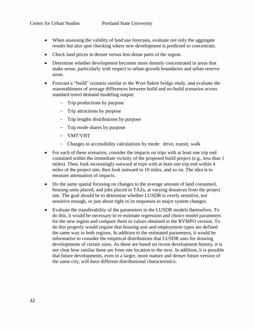
Center for Urban Studies Portland State University
42
When assessing the validity of land use forecasts, evaluate not only the aggregate
results but also spot checking where new development is predicted to concentrate.
Check land prices in denser versus less dense parts of the region.
Determine whether development becomes more densely concentrated in areas that
make sense, particularly with respect to urban-growth boundaries and urban reserve
areas.
Forecast a “build” scenario similar to the West Salem bridge study, and evaluate the
reasonableness of average differences between build and no-build scenarios across
standard travel demand modeling output:
Trip productions by purpose
Trip attractions by purpose
Trip lengths distributions by purpose
Trip mode shares by purpose
VMT/VHT
Changes in accessibility calculations by mode: drive, transit, walk
For each of these scenarios, consider the impacts on trips with at least one trip end
contained within the immediate vicinity of the proposed build project (e.g., less than 1
miles). Then, look increasingly outward at trips with at least one trip end within 4
miles of the project site; then look outward to 10 miles, and so on. The idea is to
measure attenuation of impacts.
Do the same spatial focusing on changes to the average amount of land consumed,
housing units placed, and jobs placed in TAZs, at varying distances from the project
site. The goal should be to determine whether LUSDR is overly sensitive, not
sensitive enough, or just about right in its responses to major system changes.
Evaluate the transferability of the parameters in the LUSDR models themselves. To
do this, it would be necessary to re-estimate regression and choice model parameters
for the new region and compare them to values obtained in the RVMPO version. To
do this properly would require that housing unit and employment types are defined
the same way in both regions. In addition to the estimated parameters, it would be
informative to consider the empirical distributions that LUSDR uses for drawing
developments of certain sizes. As these are based on recent development history, it is
not clear how similar these are from one location to the next. In addition, it is possible
that future developments, even in a larger, more mature and denser future version of
the same city, will have different distributional characteristics.

Center for Urban Studies Portland State University
43
7. Data for Transferability
This task is left for future research and development.

Center for Urban Studies Portland State University
44
8. Streamlined Travel Demand Model
This task is left for future research and development.

Center for Urban Studies Portland State University
45
9. Visualization Tools and Evaluation of Model Outputs
This task is left for future research and development.
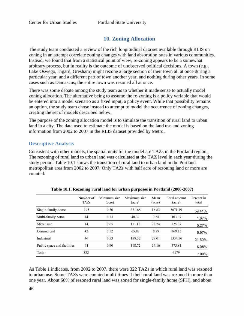
Center for Urban Studies Portland State University
46
10. Zoning Allocation
The study team conducted a review of the rich longitudinal data set available through RLIS on
zoning in an attempt correlate zoning changes with land absorption rates in various communities.
Instead, we found that from a statistical point of view, re-zoning appears to be a somewhat
arbitrary process, but in reality is the outcome of unobserved political decisions. A town (e.g.,
Lake Oswego, Tigard, Gresham) might rezone a large section of their town all at once during a
particular year, and a different part of town another year, and nothing during other years. In some
cases such as Damascus, the entire town was rezoned all at once.
There was some debate among the study team as to whether it made sense to actually model
zoning allocation. The alternative being to assume the re-zoning is a policy variable that would
be entered into a model scenario as a fixed input, a policy event. While that possibility remains
an option, the study team chose instead to attempt to model the occurrence of zoning changes,
creating the set of models described below.
The purpose of the zoning allocation model is to simulate the transition of rural land to urban
land in a city. The data used to estimate the model is based on the land use and zoning
information from 2002 to 2007 in the RLIS dataset provided by Metro.
Descriptive Analysis
Consistent with other models, the spatial units for the model are TAZs in the Portland region.
The rezoning of rural land to urban land was calculated at the TAZ level in each year during the
study period. Table 10.1 shows the transition of rural land to urban land in the Portland
metropolitan area from 2002 to 2007. Only TAZs with half acre of rezoning land or more are
counted.
Table 10.1. Rezoning rural land for urban purposes in Portland (2000-2007)
As Table 1 indicates, from 2002 to 2007, there were 322 TAZs in which rural land was rezoned
to urban use. Some TAZs were counted multi-times if their rural land was rezoned in more than
one year. About 60% of rezoned rural land was zoned for single-family home (SFH), and about

Center for Urban Studies Portland State University
47
22% was rezoned into industrial land. Since the numbers of observations (TAZs) are too small
for some urban land use types, such as multi-family home (MFH) and mixed use, to estimate
model, these urban land use types are combined into two general groups: residential and non-
residential groups. The residential group includes SFH, MFH, and mixed use. The non-
residential group has commercial, industrial, and public land use types. Mixed-use land is tricky
because it includes both residential and commercial land uses. Since most rural land is in urban
peripheral areas, and mixed-use land in those areas is mostly for residential purpose, it is
categorized into the residential group. In the following two-step models (Figure 1), residential
and non-residential groups are modeled separately.
Two-Step Rezoning Allocation Model
As shown below in Figure 10.1, the rezoning allocation process is modeled in two steps. The
first step models are binary logit models, predicting which TAZs will see the transition of rural
land to urban land, specifically, residential land and non-residential land. The second step models
are regression models, forecasting the acres of rural land in those TAZs that are going to be
rezoned into urban residential land and non-residential developable land.
Figure 10.1. Two-Step zoning allocation model
Residential Binary Logit Model
The purpose of the residential binary logit model is to estimate if some rural land in a TAZ will
be rezoned to urban residential land. Descriptive statistics and model estimation result may be
found in Tables 10.2 and 10.3, respectively.
Model results show that rural land in TAZs within the UGB is more likely to be rezoned to urban
residential land than rural land in TAZs in the UGB peripheral areas, especially those outside of
the UGB. Existing higher SFH density also increases the chance of rural land to be rezoned to
urban residential land. The variable representing employment accessibility by auto of a TAZ has
a negative sign, which is difficult to explain. However, employment accessibility by transit

Center for Urban Studies Portland State University
48
shows a positive effect on the rezoning of rural land to urban residential land. The coefficient for
the land price variable shows a marginally significant negative sign, indicating cheaper rural land
is more likely to be rezoned to urban residential land. In addition, rural land in locations with
higher employment density is less likely to be rezoned to urban residential land.
Table 10.2. Descriptive statistics of explanatory variables in the residential binary logit model
Table 10.3. Residential binary logit model results
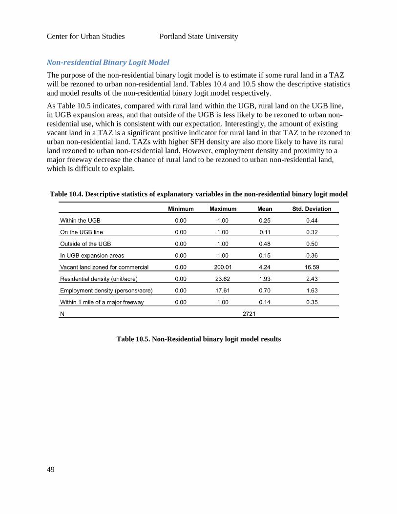
Center for Urban Studies Portland State University
49
Non-residential Binary Logit Model
The purpose of the non-residential binary logit model is to estimate if some rural land in a TAZ
will be rezoned to urban non-residential land. Tables 10.4 and 10.5 show the descriptive statistics
and model results of the non-residential binary logit model respectively.
As Table 10.5 indicates, compared with rural land within the UGB, rural land on the UGB line,
in UGB expansion areas, and that outside of the UGB is less likely to be rezoned to urban non-
residential use, which is consistent with our expectation. Interestingly, the amount of existing
vacant land in a TAZ is a significant positive indicator for rural land in that TAZ to be rezoned to
urban non-residential land. TAZs with higher SFH density are also more likely to have its rural
land rezoned to urban non-residential land. However, employment density and proximity to a
major freeway decrease the chance of rural land to be rezoned to urban non-residential land,
which is difficult to explain.
Table 10.4. Descriptive statistics of explanatory variables in the non-residential binary logit model
Table 10.5. Non-Residential binary logit model results

Center for Urban Studies Portland State University
50
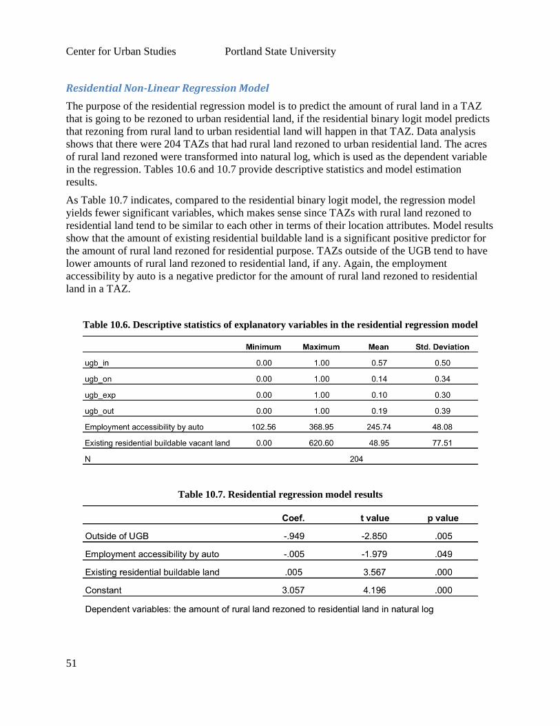
Center for Urban Studies Portland State University
51
Residential Non-Linear Regression Model
The purpose of the residential regression model is to predict the amount of rural land in a TAZ
that is going to be rezoned to urban residential land, if the residential binary logit model predicts
that rezoning from rural land to urban residential land will happen in that TAZ. Data analysis
shows that there were 204 TAZs that had rural land rezoned to urban residential land. The acres
of rural land rezoned were transformed into natural log, which is used as the dependent variable
in the regression. Tables 10.6 and 10.7 provide descriptive statistics and model estimation
results.
As Table 10.7 indicates, compared to the residential binary logit model, the regression model
yields fewer significant variables, which makes sense since TAZs with rural land rezoned to
residential land tend to be similar to each other in terms of their location attributes. Model results
show that the amount of existing residential buildable land is a significant positive predictor for
the amount of rural land rezoned for residential purpose. TAZs outside of the UGB tend to have
lower amounts of rural land rezoned to residential land, if any. Again, the employment
accessibility by auto is a negative predictor for the amount of rural land rezoned to residential
land in a TAZ.
Table 10.6. Descriptive statistics of explanatory variables in the residential regression model
Table 10.7. Residential regression model results

Center for Urban Studies Portland State University
52
Non-Residential Regression Model
The purpose of the non-residential regression model is to predict the acres of rural land in a TAZ
that is going to be rezoned to urban non-residential land, if the non-residential binary logit model
predicts that rezoning from rural land to urban non-residential land will happen in that TAZ.
Data analysis shows that there were only 89 TAZs that had rural land rezoned to urban non-
residential land from 2002 to 2007 in the Portland metropolitan area. The acres of rural land
rezoned were transformed into natural log, which is used as the dependent variable in the
regression model. Due to the small sample size, few significant predictors were obtained in many
model specifications that have been tested. Tables 10.8 and 10.9 provide descriptive statistics
and model estimation results.
As Table 10.9 indicates, only two variables were found to be significant at 10 percent level:
existing vacant land zoned for industrial purpose and population density. TAZs with more
buildable land zoned for industrial purpose and lower population density tend to have more rural
land rezoned to urban non-residential land.
Table 10.8. Descriptive statistics of explanatory variables in the non-residential regression model
Table 10.9 Residential regression model results

Center for Urban Studies Portland State University
53
Implementation Issues
In order to implement the zoning allocation model described above, the following changes would
need to be made the LUSDR program code:
A general method would need to be created to implement the 2-step procedure.
Methods would need to be created to implement each of the binary logit models to
predict whether a TAZ will have any rezoning.
Methods would need to be developed to implement each of the regression models used to
predict the number of acres of to be converted.
A method would need to be created to update the acreage of available developable
residential and non-residential land.
Further Research and Development Needed
This method does not distinguish between single- and multi-family residential uses, making it
necessary to assume that land is first rezoned to from rural to the least intense usage, that being
single-family. This method also does not distinguish between different types of non-residential
zoning when converting land from rural to developable. This requires further study; however, the
vast majority of observed cases were a conversion from rural to low-density industrial, so this
may be a reasonable starting point.
A more informed option would be to use a comprehensive plan overlay to guide the sub-category
allocation.
Yet, another option would be to utilize the historical rates of conversion found in Table 10.1 to
apportion converted residential land between single- and multi-family residential, and to
apportion converted non-residential land between commercial, industrial and public uses. In any
one TAZ, however, it may not make sense to allocate converted land to all of the non-residential
uses. For example, further consideration should be given to whether the presence of existing
industrial land in the same or nearby TAZ would make it more likely for a conversion to be
industrial.
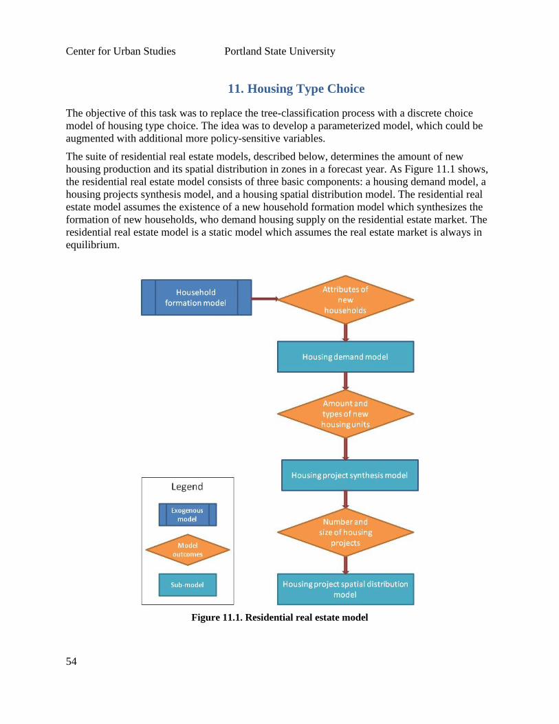
Center for Urban Studies Portland State University
54
11. Housing Type Choice
The objective of this task was to replace the tree-classification process with a discrete choice
model of housing type choice. The idea was to develop a parameterized model, which could be
augmented with additional more policy-sensitive variables.
The suite of residential real estate models, described below, determines the amount of new
housing production and its spatial distribution in zones in a forecast year. As Figure 11.1 shows,
the residential real estate model consists of three basic components: a housing demand model, a
housing projects synthesis model, and a housing spatial distribution model. The residential real
estate model assumes the existence of a new household formation model which synthesizes the
formation of new households, who demand housing supply on the residential estate market. The
residential real estate model is a static model which assumes the real estate market is always in
equilibrium.
Figure 11.1. Residential real estate model
Center for Urban Studies Portland State University
55
Housing Demand Model
Methodology
In this model, we use household attributes to decide the housing types they are going to choose.
Following Train (2003), the discrete choice location models in this study were derived as
follows. Each household is described by a vector of attributes , and they bid for housing on the
market among a range of housing types j, which is determined by three dimensional
characteristics: housing tenure , number of units in the structure , and property value level
(monthly rent is used for rental houses). For a household with a bundle of attributes , the
indirect utility function of each housing type in linear form can be written as:
where represents the utility of each housing type for a household , and represents the
parameters that measure the effects of household attributes on household tenure choice.
Assuming the error part in the utility function is independently and identically distributed, the
probability of housing type chosen by household is:
( ) ( )
∑ ( )
Input Data
As shown in Table 11.1, input data for the model includes:
Household size
Household income
Presence of kids
Number of elders (age 65+)
The data used to estimate models is from the PUMS data 2005 and 2006 for the state of Oregon.
The household attributes in the model are used as dummy variables. Considering that the
household income in different years and different regions may not be comparable, the
households in each PUMA district in each year are grouped evenly into four income categories.
This groups households into income quartiles such that households at the same income level
from different PUMA districts and years are considered to be the same, although their absolute
income number may be quite different. Descriptive statistics of household attributes are showed
in Table 11.1.
PUMS data not only provides the information about the households, but also the characteristics
of their dwellings. As mentioned above, in this model, three housing characteristics are used:
housing tenure (own or rent), structure type, and housing value (monthly rent for rental housing).
There are six housing structure types based on the number of families in the building: single
family house detached, single family house attached, mobile home, multifamily house with 2-4
units, and multifamily house with 5 or more units. In the data, housing tenure and structure types
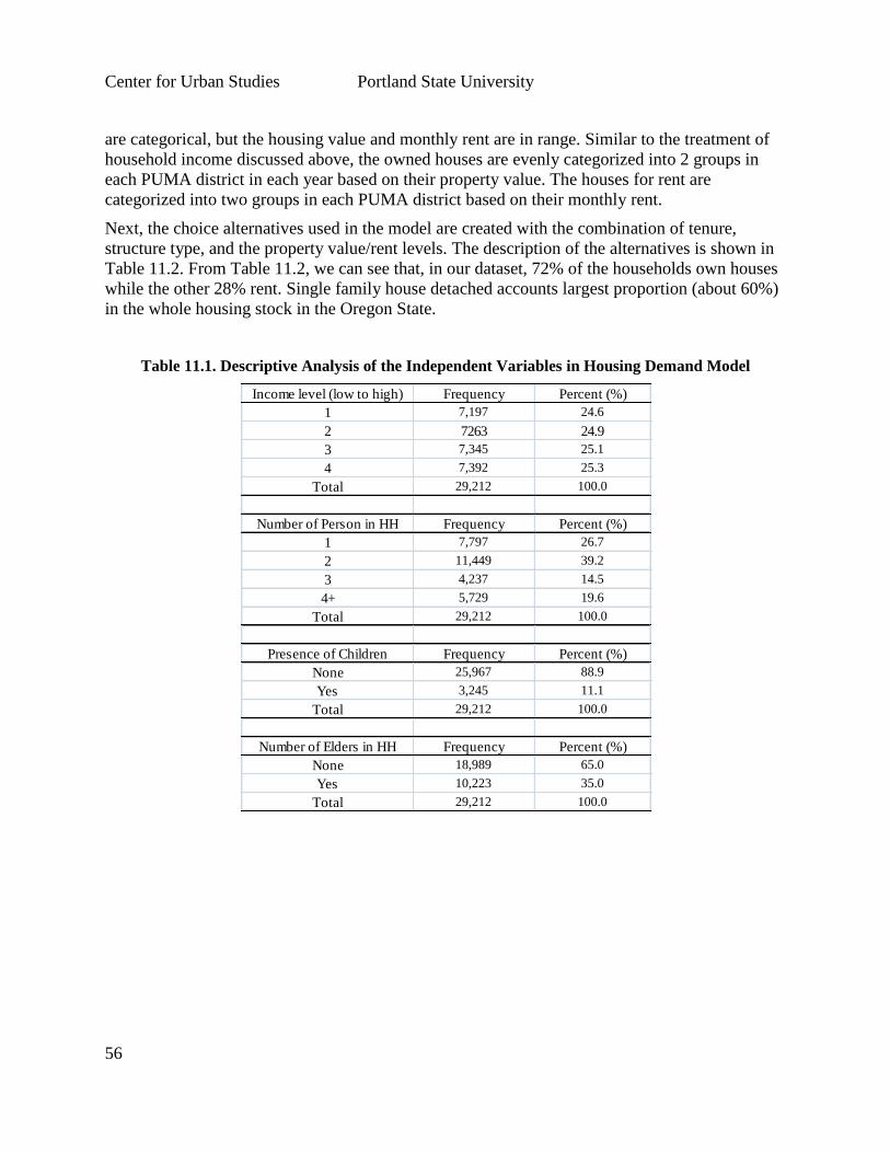
Center for Urban Studies Portland State University
56
are categorical, but the housing value and monthly rent are in range. Similar to the treatment of
household income discussed above, the owned houses are evenly categorized into 2 groups in
each PUMA district in each year based on their property value. The houses for rent are
categorized into two groups in each PUMA district based on their monthly rent.
Next, the choice alternatives used in the model are created with the combination of tenure,
structure type, and the property value/rent levels. The description of the alternatives is shown in
Table 11.2. From Table 11.2, we can see that, in our dataset, 72% of the households own houses
while the other 28% rent. Single family house detached accounts largest proportion (about 60%)
in the whole housing stock in the Oregon State.
Table 11.1. Descriptive Analysis of the Independent Variables in Housing Demand Model
Income level (low to high) Frequency Percent (%)
1 7,197 24.6
2 7263 24.9
3 7,345 25.1
4 7,392 25.3
Total 29,212 100.0
Number of Person in HH Frequency Percent (%)
1 7,797 26.7
2 11,449 39.2
3 4,237 14.5
4+ 5,729 19.6
Total 29,212 100.0
Presence of Children Frequency Percent (%)
None 25,967 88.9
Yes 3,245 11.1
Total 29,212 100.0
Number of Elders in HH Frequency Percent (%)
None 18,989 65.0
Yes 10,223 35.0
Total 29,212 100.0
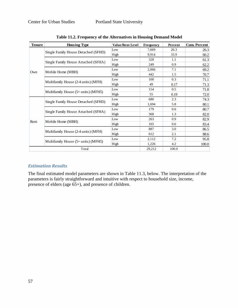
Center for Urban Studies Portland State University
57
Table 11.2. Frequency of the Alternatives in Housing Demand Model
Estimation Results
The final estimated model parameters are shown in Table 11.3, below. The interpretation of the
parameters is fairly straightforward and intuitive with respect to household size, income,
presence of elders (age 65+), and presence of children.
Tenure Housing Type Value/Rent Level Frequency Percent Cum. Percent
Low 7,669 26.3 26.3
High 9,914 33.9 60.2
Low 328 1.1 61.3
High 249 0.9 62.2
Low 2,066 7.1 69.2
High 442 1.5 70.7
Low 100 0.3 71.1
High 49 0.17 71.3
Low 154 0.5 71.8
High 55 0.19 72.0
Low 680 2.3 74.3
High 1,694 5.8 80.1
Low 179 0.6 80.7
High 368 1.3 82.0
Low 263 0.9 82.9
High 165 0.6 83.4
Low 887 3.0 86.5
High 612 2.1 88.6
Low 2,112 7.2 95.8
High 1,226 4.2 100.0
29,212 100.0
Single Family House Attached (SFHA)
Mobile Home (MBH)
Multifamily House (2-4 units) (MFH)
Multifamily House (5+ units) (MFH5)
Single Family House Detached (SFHD)
Total
Mobile Home (MBH)
Multifamily House (2-4 units) (MFH)
Multifamily House (5+ units) (MFH5)
Rent
Own
Single Family House Detached (SFHD)
Single Family House Attached (SFHA)
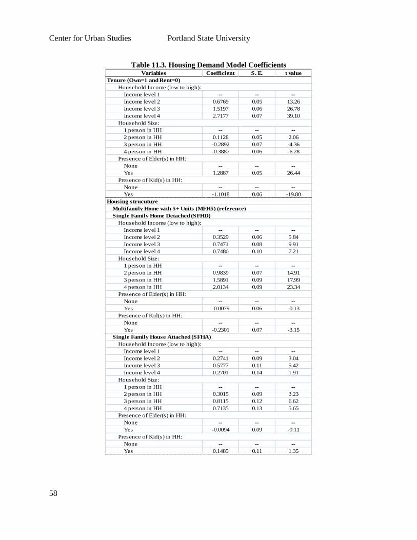
Center for Urban Studies Portland State University
58
Table 11.3. Housing Demand Model Coefficients
Variables Coefficient S. E. t value
Income level 1 -- -- --
Income level 2 0.6769 0.05 13.26
Income level 3 1.5197 0.06 26.78
Income level 4 2.7177 0.07 39.10
1 person in HH -- -- --
2 person in HH 0.1128 0.05 2.06
3 person in HH -0.2892 0.07 -4.36
4 person in HH -0.3887 0.06 -6.28
None -- -- --
Yes 1.2887 0.05 26.44
None -- -- --
Yes -1.1018 0.06 -19.80
Income level 1 -- -- --
Income level 2 0.3529 0.06 5.84
Income level 3 0.7471 0.08 9.91
Income level 4 0.7480 0.10 7.21
1 person in HH -- -- --
2 person in HH 0.9839 0.07 14.91
3 person in HH 1.5891 0.09 17.99
4 person in HH 2.0134 0.09 23.34
None -- -- --
Yes -0.0079 0.06 -0.13
None -- -- --
Yes -0.2301 0.07 -3.15
Income level 1 -- -- --
Income level 2 0.2741 0.09 3.04
Income level 3 0.5777 0.11 5.42
Income level 4 0.2701 0.14 1.91
1 person in HH -- -- --
2 person in HH 0.3015 0.09 3.23
3 person in HH 0.8115 0.12 6.62
4 person in HH 0.7135 0.13 5.65
None -- -- --
Yes -0.0094 0.09 -0.11
None -- -- --
Yes 0.1485 0.11 1.35
Tenure (Own=1 and Rent=0)
Housing strucuture
Multifamily Home with 5+ Units (MFH5) (reference)
Single Family Home Detached (SFHD)
Single Family House Attached (SFHA)
Household Income (low to high):
Household Size:
Presence of Elder(s) in HH:
Presence of Kid(s) in HH:
Household Income (low to high):
Household Size:
Presence of Elder(s) in HH:
Presence of Kid(s) in HH:
Household Income (low to high):
Household Size:
Presence of Elder(s) in HH:
Presence of Kid(s) in HH:
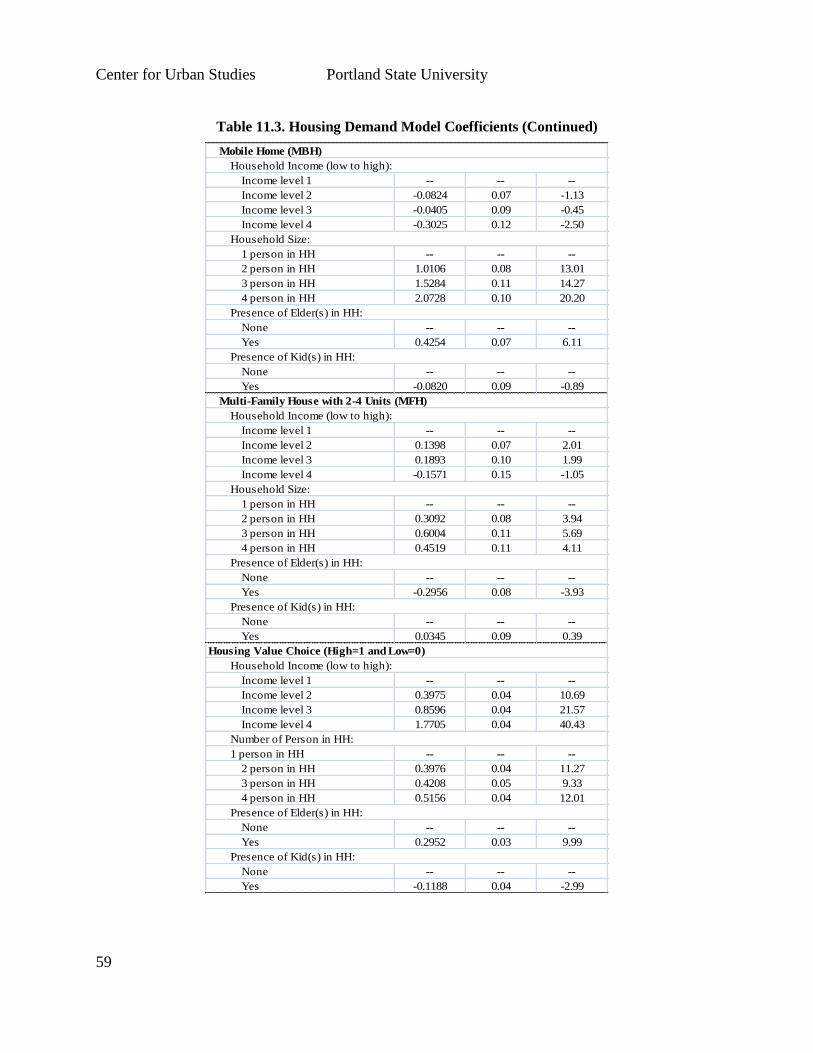
Center for Urban Studies Portland State University
59
Table 11.3. Housing Demand Model Coefficients (Continued)
Income level 1 -- -- --
Income level 2 -0.0824 0.07 -1.13
Income level 3 -0.0405 0.09 -0.45
Income level 4 -0.3025 0.12 -2.50
1 person in HH -- -- --
2 person in HH 1.0106 0.08 13.01
3 person in HH 1.5284 0.11 14.27
4 person in HH 2.0728 0.10 20.20
None -- -- --
Yes 0.4254 0.07 6.11
None -- -- --
Yes -0.0820 0.09 -0.89
Income level 1 -- -- --
Income level 2 0.1398 0.07 2.01
Income level 3 0.1893 0.10 1.99
Income level 4 -0.1571 0.15 -1.05
1 person in HH -- -- --
2 person in HH 0.3092 0.08 3.94
3 person in HH 0.6004 0.11 5.69
4 person in HH 0.4519 0.11 4.11
None -- -- --
Yes -0.2956 0.08 -3.93
None -- -- --
Yes 0.0345 0.09 0.39
Income level 1 -- -- --
Income level 2 0.3975 0.04 10.69
Income level 3 0.8596 0.04 21.57
Income level 4 1.7705 0.04 40.43
1 person in HH -- -- --
2 person in HH 0.3976 0.04 11.27
3 person in HH 0.4208 0.05 9.33
4 person in HH 0.5156 0.04 12.01
None -- -- --
Yes 0.2952 0.03 9.99
None -- -- --
Yes -0.1188 0.04 -2.99
Household Income (low to high):
Number of Person in HH:
Presence of Elder(s) in HH:
Presence of Kid(s) in HH:
Multi-Family House with 2-4 Units (MFH)
Household Income (low to high):
Household Size:
Presence of Elder(s) in HH:
Presence of Kid(s) in HH:
Housing Value Choice (High=1 and Low=0)
Mobile Home (MBH)
Household Income (low to high):
Household Size:
Presence of Elder(s) in HH:
Presence of Kid(s) in HH:

Center for Urban Studies Portland State University
60
Table 11.3. Housing Demand Model Coefficients (Continued)
Owned SFHD with low value -0.7033 0.04 -15.85
Owned SFHD with high value -1.8469 0.06 -32.51
Owned SFHA with low value -3.2173 0.10 -33.71
Owned SFHA with high value -4.6260 0.12 -39.70
Owned MBH with low value -1.7476 0.06 -28.83
Owned MBH with high value -4.4611 0.09 -49.40
Owned MFH with low value -4.0333 0.12 -33.13
Owned MFH with high value -5.8260 0.17 -33.53
Owned MFH5 with low value -3.5179 0.09 -37.78
Owned MFH5 with high value -5.5629 0.15 -36.00
Rent SFHD with low value -2.1131 0.06 -33.32
Rent SFHD with high value -2.0892 0.06 -32.98
Rent SFHA with low value -2.8836 0.10 -29.62
Rent SFHA with high value -2.7860 0.09 -30.65
Rent MBH with low value -2.9035 0.08 -34.33
Rent MBH with high value -4.0959 0.11 -38.95
Rent MFH with low value -1.0447 0.06 -17.91
Rent MFH with high value -2.0325 0.07 -28.08
Rent MFH5 with low value -- -- --
Rent MFH5 with high value -1.0930 0.04 -25.35
Number of paprameters
Log likelihood at constant
Log likelihood at convergence
Rho-square
Adjusted Rho-square
Number of observations
Alternative Specific Constants
67
-59878
-53713
0.10
0.10
29212

Center for Urban Studies Portland State University
61
Housing Project Synthesis Model
Due to data limitation, different types of housing units forecasted by the housing demand model
are aggregated into two types: single family home (SFH) and multi-family home (MFH). SFH
refers to single family detached home, while MFH represents any attached housing structure,
including single family attached homes and multi-units apartments and condos. A SFH project
consists of all SFH units in a zone developed by the same developer in a single year. A SFH
project consists of all MFH units in a zone developed by the same developer in a single year.
SFH and MFH project synthesis models are developed based on the housing permit data from
2000 to 2006. The 2007 data is hold to measure the performance of these models. The housing
permit data was provided by Metro, the regional government for the Portland Metropolitan Area.
Synthesized SFH and MFH projects are used as forecasting units for new housing location
choice forecast models.
Size Distributions of SFH and MFH Projects
Our tests show that Gamma distribution fits the size distributions of SFH and MFH projects best
among many probability distributions that have been tried. The gamma distribution is a two-
parameter family of continuous probability distributions. It has a shape parameter and a scale
parameter . The equation defining the probability density function of a gamma-distributed
random variable is:
( )
⁄
( ) for and
Here, the random variable represents project size. Figures 11.2 and 11.3 show the Gamma Q-Q
plots for the sizes of SFH and MFH projects, respectively, from 2000 to 2007 in the Portland
metropolitan region.
Data Input for SFH and MFH Project Synthesis
To synthesize SFH and MFH projects in a forecast year based on their size distributions in
previous years, the following information is needed:
Total amount of new SFH/MFH units in the forecast year. This can be forecasted by the
housing demand model.
Size distributions of SFH and MFH projects (specifically, the shape and scale parameters
of the Gamma distribution).
In this model, we assume the size distribution of housing projects is stable across years.
The shape and scale parameters of the Gamma distribution can be estimated based on
housing project sizes in previous years.
Minimum and maximum sizes of SFH/MFH projects in the forecast year.
In this model, the minimum sizes for SFH and MFH projects are 1 unit and 2 units
separately. The largest sizes for SFH and MFH projects in previous years can be used as
the maximum sizes for SFH and MFH projects in the forecast year.

Center for Urban Studies Portland State University
62
Total number of SFH/MFH projects in the forecast year.
In order to control the number of synthesized projects in the forecast year and make it
more realistic, the numbers of SFH and MFH projects in the forecast year are estimated
by dividing the total number of new SFH/MFH units by their mean sizes in previous
years. In order to make the synthesis models converge very quickly, a tolerance number
is set for the total number of SFH/MFH projects in the forecast year. In this report, the
tolerance is set as 5.
Since synthesized housing projects are generated randomly, the model results will not be exactly
the same each time the model is run. However, since each set of projects synthesized by the same
model is imposes the same constraints, such as the total number of housing units, minimum and
maximum project sizes, probability distribution, and number of the projects, they tend to be very
similar to each other.
Figure 11.2. Size Distribution of SFH Projects in Portland Metropolitan Area (2000-2007)
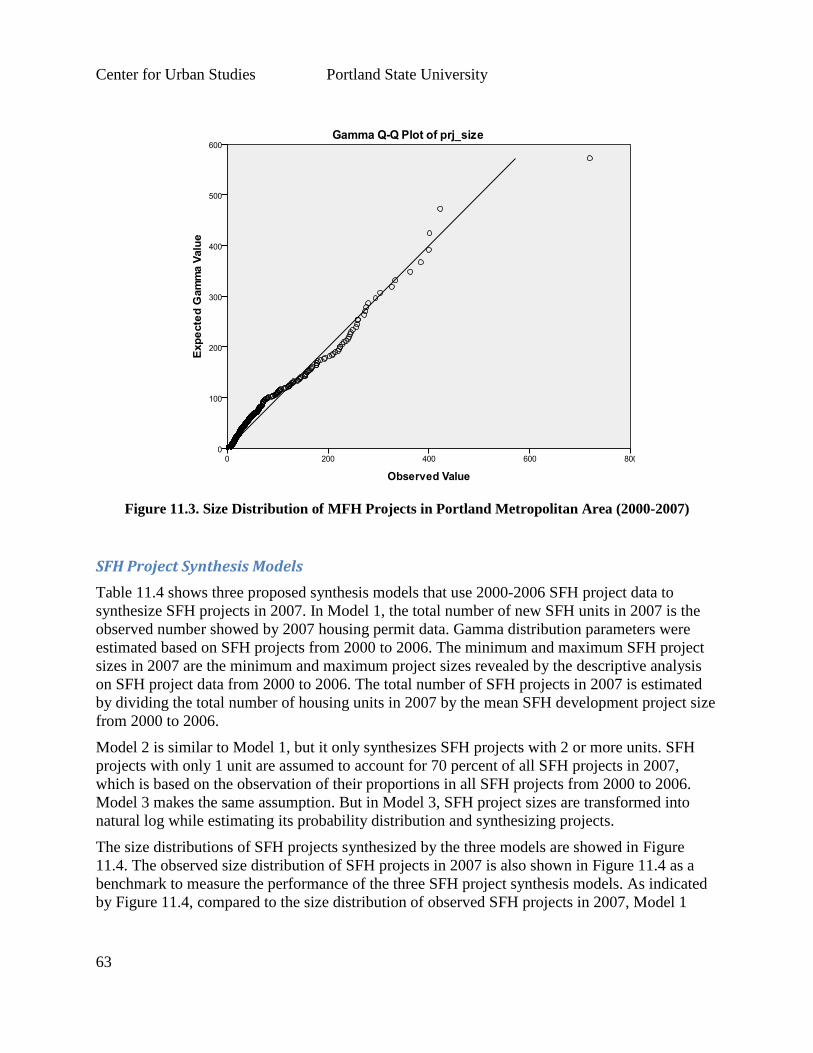
Center for Urban Studies Portland State University
63
Figure 11.3. Size Distribution of MFH Projects in Portland Metropolitan Area (2000-2007)
SFH Project Synthesis Models
Table 11.4 shows three proposed synthesis models that use 2000-2006 SFH project data to
synthesize SFH projects in 2007. In Model 1, the total number of new SFH units in 2007 is the
observed number showed by 2007 housing permit data. Gamma distribution parameters were
estimated based on SFH projects from 2000 to 2006. The minimum and maximum SFH project
sizes in 2007 are the minimum and maximum project sizes revealed by the descriptive analysis
on SFH project data from 2000 to 2006. The total number of SFH projects in 2007 is estimated
by dividing the total number of housing units in 2007 by the mean SFH development project size
from 2000 to 2006.
Model 2 is similar to Model 1, but it only synthesizes SFH projects with 2 or more units. SFH
projects with only 1 unit are assumed to account for 70 percent of all SFH projects in 2007,
which is based on the observation of their proportions in all SFH projects from 2000 to 2006.
Model 3 makes the same assumption. But in Model 3, SFH project sizes are transformed into
natural log while estimating its probability distribution and synthesizing projects.
The size distributions of SFH projects synthesized by the three models are showed in Figure
11.4. The observed size distribution of SFH projects in 2007 is also shown in Figure 11.4 as a
benchmark to measure the performance of the three SFH project synthesis models. As indicated
by Figure 11.4, compared to the size distribution of observed SFH projects in 2007, Model 1

Center for Urban Studies Portland State University
64
tends to overestimate SFH projects with 1 unit and underestimate the SF projects with 2 units. As
mentioned above, in Model 2, only the SFH projects with 2 or more units are synthesized.
Figure 11.4 shows that Model 2 overestimates the number of SFH projects with 2-5 units.
Compared to Models 1 and 2, size distribution of SFH projects synthesized by Model 3 is closer
to the observed SFH projects in 2007, indicating that this model has the best performance in the
three models. Thus this model is selected as the final model and SFH projects synthesized by this
model are used as forecasting units for the SFH location choice models.
MFH Project Synthesis Models
Table 11.5 shows the three synthesis models that use 2000-2006 MFH project data to synthesize
MFH projects in 2007. Model 1 is the base model. The total number of new MFH units is the
observed number in 2007. The number of MFH projects is calculated by dividing the total new
MFH unit in 2007 by the mean size of MFH projects from 2000 to 2006. Similar to SFH
projects, the mean size of MFH projects dropped in 2007, making the estimated number of MFH
projects in 2007 smaller than the observed number.
Descriptive analysis shows that there were only 9 MFH projects whose sizes were larger than
300 units from 2000 to 2006, so they are treated as outliers and the maximum project size in the
forecast year is set as 300 units.
Model 2 is different from Model 1 in that MFH project sizes were transformed into natural log
while estimating the shape and scale parameters for Gamma distribution. Model 3 does that too.
But different from Model 2, MFH projects with 2 units are not synthesized in Model 3. Their
proportion in the total number of MFH projects in 2007 was assumed to be 30 percent, as
observed from previous years.
Figure 11.5 compares the size distributions of MFH projects synthesized by the three models and
observed in 2007. As the figure shows, the size distribution of MFH projects synthesized by
Model 3 is closest to the size distribution of observed MFH projects in 2007. Thus model 3 is
selected as the MFH project synthesis model and MFH projects synthesized by Model 3 are used
as forecasting units for the MFH location choice models.
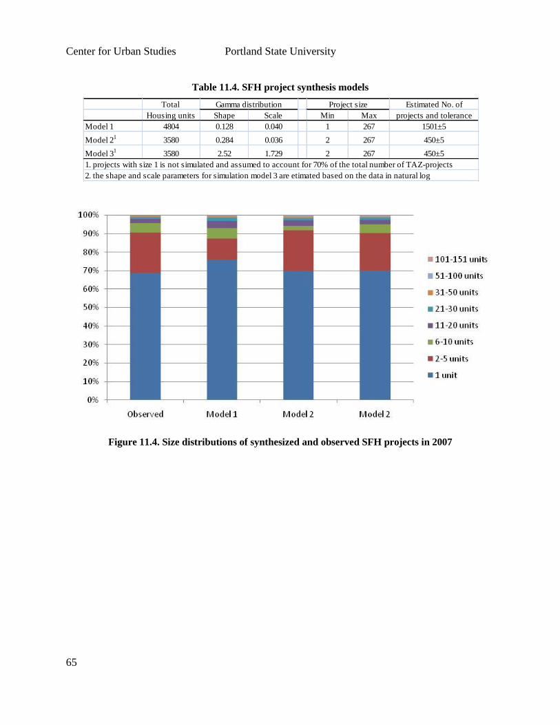
Center for Urban Studies Portland State University
65
Table 11.4. SFH project synthesis models
Figure 11.4. Size distributions of synthesized and observed SFH projects in 2007
Total Estimated No. of
Housing units Shape Scale Min Max projects and tolerance
Model 1 4804 0.128 0.040 1 267 1501±5
Model 21
3580 0.284 0.036 2 267 450±5
Model 31
3580 2.52 1.729 2 267 450±5
Gamma distribution Project size
2. the shape and scale parameters for simulation model 3 are etimated based on the data in natural log
1. projects with size 1 is not simulated and assumed to account for 70% of the total number of TAZ-projects
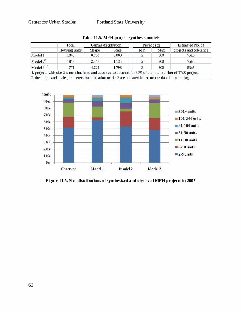
Center for Urban Studies Portland State University
66
Table 11.5. MFH project synthesis models
Figure 11.5. Size distributions of synthesized and observed MFH projects in 2007
Total Estimated No. of
Housing units Shape Scale Min Max projects and tolerance
Model 1 1843 0.198 0.008 2 300 75±5
Model 22
1843 2.347 1.134 2 300 75±5
Model 31,2
1771 4.725 1.798 3 300 53±5
Gamma distribution Project size
2. the shape and scale parameters for simulation model 3 are etimated based on the data in natural log
1. projects with size 2 is not simulated and assumed to account for 30% of the total number of TAZ-projects
Center for Urban Studies Portland State University
67
Housing Project Location Choice Model
Methodology
Discrete choice modeling techniques were used to reveal the compensatory tradeoffs that
developers make when choosing sites for their housing projects among a set of alternative
locations. Each individual makes a choice from a set of alternatives assumed to be available to
them. However, it was neither computationally feasible nor theoretically realistic to assume that
developers would consider all 1,348 TAZs in the region as alternatives in the choice set for each
project. For each SFH project, given that most SFH developments were built on vacant buildable
land, we used a random sample of 49 alternative TAZs from TAZs that had enough buildable
land for it, plus the chosen TAZ as the choice set for it. For each MFH project, we used a random
sample of 49 alternative TAZs from all 1,348 TAZs, plus the chosen TAZ as the choice set for it.
Alternatives were sampled without replacement and without any type of importance sampling or
stratification.
Following Train (2003), the discrete choice location models in this study are derived as follows.
Each developer faces a choice among alternative locations. The developer obtains a certain
level of utility from each alternative location, and the utility is composed of two parts, the
systematic portion and the error :
For each alternative location , we have a set of alternative specific location attributes .
Assuming that the error in utility function is identically and independently distributed (IID)
across alternatives and to follow a Gumbel distribution, the choice probability for alternative
TAZ is:
( ) ( )
∑ ( )
where denotes the parameters for each TAZ attribute. The discrete choice models developed
under these assumptions are called MNL models.
Data Inputs
The following TAZ attributes (shown in Table 11.6) are used to locate SFH and MFH projects
into zones:
Relative location to the Urban Growth Boundary (UGB).
Transportation accessibility: The calculation of transportation accessibility was based on
the modeled morning two-hour peak travel times for pairs of TAZs, utilizing a static
estimate of 2005 congested network travel times. The Metro travel demand model also
provides 2005 estimates of employment by TAZ and by industry sector. We adapted the
negative exponential travel impedance formula from Meyer and Miller (2001, p. 336):
Center for Urban Studies Portland State University
68
(∑ ( )
)
in which measures the employment accessibility for TAZ , β is a parameter
indicating the sensitivity of trip making to travel time, is the travel time from TAZ to
TAZ , and is the number of jobs in TAZ . With this formula, we calculated
transportation accessibilities by auto and transit modes for employment purpose in each TAZ. To
account for their non-linear effects, both auto and transit accessibilities were used in natural log
form in models.
Infrastructure density (lineal meters/square km): Density of roads is used to represent the
level of infrastructure concentration in each TAZ, which was calculated by dividing the
total length of roads in a TAZ over the area of the TAZ. To account for its non-linear
effect, natural log was taken when it was included in models.
Residential density: SFH/MFH net densities were calculated as the total number of
SFH/MFH units divided by the total land area they actually occupied. Rather than using
these density measures directly, we found more statistically significant correlations with
location choices by grouping them into categories as shown in Table 11.6.
Housing diversity: To measure housing diversity in each TAZ, the ratio of MFH units to
SFH units in each TAZ was calculated and TAZs were grouped into three categories
based on the ratio: TAZs dominated by SFHs, TAZs with mixed housing, and TAZs
dominated by MFHs, as shown in Table 11.6.
Mixed use: We used the ratio of the number of retail employees to the number of housing
units to measure each TAZ’s mixed-use level. As shown in Table 11.6, based on this
ratio, TAZs were categorized into three roughly even groups based on their levels of
mixed-use.
Buildable land: For SFH developments, the availability of buildable land in each TAZ is
the area of vacant land zoned for low-density residential use and suitable for building
houses. For MFH developments, the availability of buildable land in each TAZ is the area
of vacant land zoned for medium- and high-density residential purposes or mixed-use
purpose.
Median household income
Average household size
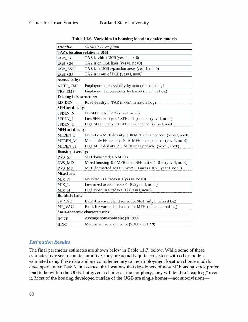
Center for Urban Studies Portland State University
69
Table 11.6. Variables in housing location choice models
Estimation Results
The final parameter estimates are shown below in Table 11.7, below. While some of these
estimates may seem counter-intuitive, they are actually quite consistent with other models
estimated using these data and are complementary to the employment location choice models
developed under Task 5. In essence, the locations that developers of new SF housing stock prefer
tend to be within the UGB, but given a choice on the periphery, they will tend to “leapfrog” over
it. Most of the housing developed outside of the UGB are single homes—not subdivisions—
Variable Variable description
UGB_IN TAZ is within UGB (yes=1, no=0)
UGB_ON TAZ is on UGB lines (yes=1, no=0)
UGB_EXP TAZ is in UGB expansion areas (yes=1, no=0)
UGB_OUT TAZ is is out of UGB (yes=1, no=0)
Accessibility:
AUTO_EMP Employment accessibility by auto (in natural log)
TRS_EMP Employment accessibility by transit (in natural log)
RD_DEN Road density in TAZ (m/km2, in natural log)
SFDEN_N No SFH in the TAZ (yes=1, no=0)
SFDEN_L Low SFH density: < 1 SFH unit per acre (yes=1, no=0)
SFDEN_H High SFH density: 6+ SFH units per acre (yes=1, no=0)
MFDEN_L No or Low MFH density: < 10 MFH units per acre (yes=1, no=0)
MFDEN_M Medium MFH density: 10-20 MFH units per acre (yes=1, no=0)
MFDEN_H High MFH density: 21+ MFH units per acre (yes=1, no=0)
DVS_SF SFH dominated; No MFHs
DVS_MIX Mixed housing: 0 < MFH units/SFH units <= 0.5 (yes=1, no=0)
DVS_MF MFH dominated: MFH units/SFH units > 0.5 (yes=1, no=0)
Mixed use:
MIX_N No mixed use: index = 0 (yes=1, no=0)
MIX_L Low mixed use: 0< index <= 0.2 (yes=1, no=0)
MIX_H High mixed use: index > 0.2 (yes=1, no=0)
SF_VAC Buildable vacant land zoned for SFH (m2
, in natural log)
MF_VAC Buildable vacant land zoned for MFH (m2, in natural log)
HSIZE Average household size (in 1999)
HINC Median household income ($1000) (in 1999)
Socio-economic characteristics :
Buildable land:
TAZ's location relative to UGB:
SFH net density:
MFH net density:
Housing diversity:
Existing infrastructure:

Center for Urban Studies Portland State University
70
developed on lots of two acres and greater. The UGB does not play a role in the MF location
choice model since all eligible MF developable land is by regulation within the UGB.
Table 11.7. SFH and MFH projects location choice model coefficients
Variable
Coeff. Coeff/S.E. Coeff. Coeff/S.E.
Relative location to UGB:
UGB_IN -- -- -- --
UGB_ON -0.3888 -9.41 -- --
UGB_EXP -0.5900 -9.45 -- --
UGB_OUT -0.1361 -3.02 -- --
Accessibility:
AUTO_EMP -2.4907 -48.13 0.7001 2.94
TRS_EMP -0.0338 -6.88 -0.1059 -4.02
Existing infrastructure:
RD_DEN 0.2781 13.67 0.6793 10.01
SFH net density:
SFDEN_N -- -- -- --
SFDEN_L 0.5912 15.63 -- --
SFDEN_H 0.9340 21.39 -- --
MFH net density:
MFDEN_M -- -- -- --
MFDEN_L -0.1770 -8.01 0.5340 5.31
MFDEN_H 0.0690 2.16 1.1233 10.60
Housing diversity:
DVS_MIX -- -- -- --
DVS_SF -0.0736 -3.50 -- --
DVS_MF -0.1483 -6.06 0.6058 8.51
Mixed use:
MIX_N -- -- -- --
MIX_L -- -- -0.5885 -4.90
MIX_H -- -- -0.1840 -2.86
Buildable land:
SF_VAC 0.0429 5.23 -- --
MF_VAC -- -- 0.7963 31.39
Socio-economic
characteristics:HSIZE 0.1679 4.45 -0.6330 -6.85
HINC 0.0084 12.46 -- --
SFH model MFH model
Center for Urban Studies Portland State University
71
The accessibility variables in the model are negative for new residential development, which
may seem counter-intuitive; however, this seems to be related to choosing new housing locations
that are away from commercial development. One exception is that auto access to employment is
a desirable trait for multi-family housing, through transit access to employment is seen as a
negative. An alternative interpretation is that the zones most likely to be zoned for new
residential development are of lower bid value, relative to zones that are already densely settled
and/or contain a large amount of commercial development. An additional consideration is that
the UGB offsets the negative effects of the accessibility variables to a large degree, both in terms
of utility but also in restricting the supply of available land far from employment. In essence,
within the UGB, one is never very far from employment and commercial activity.
Implementation Issues
Several changes would need to be made to LUSDR’s program code to implement the suite of
housing choice models described above:
The housing demand model would replace the current classification and regression tree
methods with a multinomial logit structure, applying Monte Carlo draws to pick an
outcome.
While sampling of zone alternatives was used for model estimation, it is more
theoretically correct to use the full set of available zones as choice alternatives
when applying these models in the simulation. This can be done efficiently in R
by calculating utilities and probabilities in arrays, using linear algebra.
The housing project synthesis model would necessitate the creation of methods to:
Implement the project size distribution function (gamma formulation)
Draw housing projects by size from the distribution function and create synthetic
housing projects
The housing project location choice model would require the implementation of
multinomial logit models for each housing type (SF and MF)
Center for Urban Studies Portland State University
72
12. Development Degradation and Redevelopment
The objective of this task was to reflect the possibility of redevelopment, which necessitates
simulating the degradation of buildings over time. Implementing a development degradation
approach in LUSDR is somewhat problematic because, in its current form, land supply is
accounted for and tracked at the TAZ level, and individual development clusters are not
maintained as distinguishable units once they are allocated to a TAZ. Moreover, there does not
seem to be a statistically valid way to estimate the amount of re-developable land within a TAZ
based on aggregate supply attributes.
The method considered here is loosely based on an approach similar to that used in UrbanSim at
a more disaggregate (parcel) level. For a developer to consider locating a proposed new
development cluster on the site, the costs of building acquisition and demolition are added to the
cost of new construction. These total construction cost must be less than the anticipated
improved value of the new structures to be built. The premise is that, as the ratio of the
improvement-value-to-land-value of a particular development drops below a certain threshold, it
becomes a candidate for redevelopment. Establishing that threshold ratio is subject to model
calibration and testing.
For the ratio of the improvement-value-to-land-value to drop, either the value of the land must be
increasing faster than the improved value, or the improved value must be dropping relative to the
land value. The first dynamic—land value increasing over time—can be simulated by applying a
land price model like those proposed in Task 1. The second dynamic—the improved value of
land dropping—could reflect the depreciated value of structures and/or a drop in the utilization
rate of those structures, i.e., higher vacancies, neither of which are modeled in the current version
of LUSDR. LUSDR does not currently maintain a year (vintage) for structures, nor does it model
current building tenants moving in or out. Of the two, building occupancy is most directly
relevant to value because it reflects income generating rents, which may be quite high even in
older buildings, and most of these have been remodeled.
Given this starting point, a good first step might be to focus on the changes in land values that
would presumably result from increased densities as LUSDR simulates period-by-period
development. Adding a module that allows movement of households and employment that have
already been placed in a previous modeling period is desirable, but is not trivial and could be
added in the future if needed.
Proposed Algorithm
Implementation of this approach is predicated on the ability of the model to carry records of sited
developments and maintain their attributes throughout the simulation. The proposed algorithm
has the following elements:
For each development cluster, calculate the improved value, using LUSDR’s current
methods of creating development cluster type distributions from tax assessor’s data to
derive a median value per square foot. Store this calculated improvement value, along
with other site attributes.

Center for Urban Studies Portland State University
73
In the absence of a model that allows households and persons to move, assume that the
occupancy of the site remains stable. Instead, apply a depreciation rate that reduces the
improved value of building structures, based on when the development entered the
simulation (e.g. year 1, year 5,…, year 25, etc.). The depreciation rate should be subject
to calibration and testing, but a useful upper bound (highest rate) would be to use the
IRS’s standard rate of 27.5 years as being the useful life of a buildings. A slower rate
that would allow for the possibility of remodeling is probably more realistic.
At the beginning of each simulation period, calculate the value of all developable land,
applying a land pricing model, such as the hedonic models described under Task 1. This
will provide a median value for residential, commercial and industrial land that will
reflect current-period residential and employment densities as well as accessibility.
Assume that this per unit value ($/acre) applies to all development clusters assigned to
the TAZ of the same usage type.
For each stored development cluster assigned to the TAZ, calculate the improvement-
value-to-land-value ratio (IVLV). Consider land development clusters that have an IVLV
below a certain threshold as being candidates for redevelopment and allow them to be
entered into the developable land supply. Selecting the right threshold values should be
developed through calibration and testing, but should be set low enough to account for
the extra development costs. As some communities offer grants to foster redevelopment,
these extra costs may not be a big issue and are probably not worth modeling in detail.
Rather than assuming that all eligible development clusters in a TAZ are eligible for
redevelopment, select a portion of them at random, weighted by the inverse of IVLV. The
proportion to select should be set to help control the pace of redevelopment. If an existing
development cluster is selected for redevelopment, the residents or employment clusters
that have been previously assigned to it are then returned to the queue to be placed once
again during the next model period.
Implementation Issues
To implement this method in LUSDR, the following major code changes would need to be made:
It would be necessary to maintain records of development clusters after they have been
allocated to zones, probably using an R data frame. These records need to include the
cluster or building type, number of residential units, non-residential square feet, acres of
land consumed by the development, and improvement value (beginning and current
period).
Create comparable development cluster records for the base-year’s existing development,
and store them in the same R data frame. This could be a tall order, but it necessary to
make this work. Each development record would need to be identified geographically by
its TAZ ID, but it would not be necessary to provide spatial coordinates below this level.
A method would need to be created to calculate improvement value depreciation and
IVLV.

Center for Urban Studies Portland State University
74
A method would need to be created to identify properties the fall below the IVLV
threshold value, randomly select development clusters to be redeveloped, and add their
acreage to the developable land supply. The method should also add the selected
development clusters’ households and employment to the location placement queue for
the next simulation period.

Center for Urban Studies Portland State University
75
Appendix A
landFrag function Source Code (Author: Joshua Roll)
#Function that takes candidate Tazs and determines fragmentation in order to decide whether
#the particular development will fit in that Taz
landFrag<-function(LandFragData_,LocModelCandidates,Dev..At){
#Setup function data
#Look up vacancy in square feet of candidate Tazs
CandidateVac.Ft_<-list()
BinData_<-LandFragData_$BinData_
IsCandTaz_<-list()
TazFeet.Zn<-
data.frame(Taz=LandFragData_$TazFeet.Zn[,1],VacantFt=LandFragData_$TazFeet.Zn[,2])
TazAcres.Zn<-
data.frame(Taz=LandFragData_$TazFeet.Zn[,1],VacantAcres=LandFragData_$TazFeet.Zn[,2])
#Compile list of candidates TAZs area
for(i in 1:length(LocModelCandidates$Taz)){
#Renames Location Choice Model generated TAZ's object
CandidateVac.Zn.X<-LocModelCandidates$Taz[i]
#Converts Development size from main script to Development density function
format
DevSize.X<-Dev..At$TotArea
#Determines vacant square feet by Location Choice Model TAZ
Vacancy.Ft<-TazFeet.Zn$VacantFt[TazAcres.Zn$Taz==CandidateVac.Zn.X]
#Creates vector of vacant square feet in TAZs with adaquate space for
development
if(Vacancy.Ft>=DevSize.X){
CandidateVac.Ft_[[i]]<-Vacancy.Ft
names(CandidateVac.Ft_[[i]])<-CandidateVac.Zn.X
}
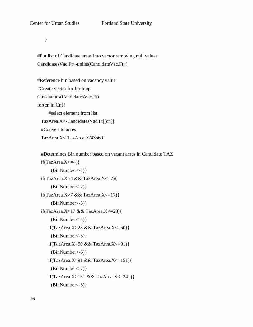
Center for Urban Studies Portland State University
76
}
#Put list of Candidate areas into vector removing null values
CandidatesVac.Ft<-unlist(CandidateVac.Ft_)
#Reference bin based on vacancy value
#Create vector for for loop
Cn<-names(CandidatesVac.Ft)
for(cn in Cn){
#select element from list
TazArea.X<-CandidatesVac.Ft[[cn]]
#Convert to acres
TazArea.X<-TazArea.X/43560
#Determines Bin number based on vacant acres in Candidate TAZ
if(TazArea.X<=4){
(BinNumber<-1)}
if(TazArea.X>4 && TazArea.X<=7){
(BinNumber<-2)}
if(TazArea.X>7 && TazArea.X<=17){
(BinNumber<-3)}
if(TazArea.X>17 && TazArea.X<=28){
(BinNumber<-4)}
if(TazArea.X>28 && TazArea.X<=50){
(BinNumber<-5)}
if(TazArea.X>50 && TazArea.X<=91){
(BinNumber<-6)}
if(TazArea.X>91 && TazArea.X<=151){
(BinNumber<-7)}
if(TazArea.X>151 && TazArea.X<=341){
(BinNumber<-8)}

Center for Urban Studies Portland State University
77
if(TazArea.X>341 && TazArea.X<=651){
(BinNumber<-9)}
if(TazArea.X>651){
(BinNumber<-10)}
#Lookup probability within bin data frames. Process determines probability of locating
development
#within its each of the candidate Tazs
for(j in 1:10){
if(BinNumber==j)
if(DevSize.X > BinData_[[j]][ length(BinData_[[j]][,1]) ,1])
TazProb.X = list(Taz=cn,Prob=0.0) else
TazProb.X=list(Taz=cn,Prob=BinData_[[j]][findInterval(DevSize.X,BinData_[[j]][,1])+1,2])
}
#Create a random number
RndNum=runif(1,min=0,max=1)
#Create list with Candidate tazs that have probabilities larger than randomly generated
number
IsCandTaz_[[cn]]<-TazProb.X$Taz[TazProb.X$Prob>RndNum]
}
#Put Candidates Tazs that made it through Land fragmentation procedure pact with rural
designation
Candidates <- list(Taz=names(IsCandTaz_),IsRural=LocModelCandidates$IsRural)
Candidates
}
Center for Urban Studies Portland State University
78
Appendix B
Manuscript begins on the next page.
Citation:
Dong, Hongwei and John Gliebe. Forecasting Location of New Housing in Integrated Models of
Land Use: Perspectives of Developers in the Portland, Oregon, Region. Transportation Research
Record: Journal of the Transportation Research Board, No. 2255. TRB, National Research
Council, Washington, D.C., 2011: 79-90.