research collection49121/... · diss. eth no. 23283 gpu accelerated implementations of a...
TRANSCRIPT

Research Collection
Doctoral Thesis
GPU accelerated implementations of a generalized eigenvaluesolver for Hermitian matrices with systematic energy and time tosolution analysis
Author(s): Solcà, Raffaele G.
Publication Date: 2016
Permanent Link: https://doi.org/10.3929/ethz-a-010656066
Rights / License: In Copyright - Non-Commercial Use Permitted
This page was generated automatically upon download from the ETH Zurich Research Collection. For moreinformation please consult the Terms of use.
ETH Library

DISS. ETH NO. 23283
GPU Accelerated Implementations of a
Generalized Eigenvalue Solver for
Hermitian Matrices with Systematic Energy
and Time to Solution Analysis
A thesis submitted to attain the degree of
DOCTOR OF SCIENCES of ETH ZURICH
(Dr. sc. ETH Zurich)
presented by
Raffaele Giuseppe Solca
Master of Science, ETH Zurich
born on 20.02.1986
citizen of Coldrerio TI
accepted on the recommendation of
Prof. Dr. Thomas C. Schulthess, examiner
Dr. Azzam Haidar, co-examiner
Prof. Dr. Joost VandeVondele, co-examiner
2016


Abstract
Density functional calculations are used to compute the properties of materials,
which can be stored in a database for later use, or used on the fly in the screening
phase of the material designing process. Since during the screening process,
the properties of a large number of materials have to be computed, the time
and the resources needed for all the simulations have to be minimized. The
time to solution of density functional calculation is dominated by dense matrix
operations, and in particular the generalized eigenvalue solver, for which new
implementations have to be developed in order to exploit the performance of the
emerging hybrid CPU+GPU supercomputers.
In the first part we present the algorithms used by the generalized eigenvalue
solver, as well as the one-stage and two-stage approach for the tridiagonaliza-
tion step, and their implementations for single-node hybrid CPU+GPU. The
performance measurements of the solver show a significant speed-up of the hy-
brid solver compared to the state-of-art CPU-only implementations. This further
show that the two-stage approach is preferable, especially when only a fraction of
the eigenspace has to be computed. The implementation is then extended to sup-
port the single node multi-GPU architecture, and its benchmark show a good
performance and scalability. We then present the implementation for the dis-
tributed memory hybrid CPU+GPU architecture of the generalized eigensolver,
as well as its performance measurements.
In the second part of the thesis we develop a model for the time to solution
and the energy to solution for distributed memory applications, which explains
the affine relationship between the resource time and the energy to solution
empirically observed previously for two stencil based algorithms. This model
shows that the affine relationship holds for different classes of algorithms, among
which linear algebra solvers are included. Furthermore we study quantitatively
the measured performance of the eigensolver, using an error analysis based on
Bayesian inference. The results of the analysis allow us to extract two parameters
which depends on the algorithm and the underlying architecture used to perform
the calculation.
The first parameter is the dynamic energy, and its scaling corresponds to the
complexity of the underlying algorithm. The second parameter represents the
static power consumed by the system, which has a strong dependence on the
architecture and the parallelization scheme.
iii

iv

Riassunto
Le simulazioni basate sulla teoria del funzionale della densita sono utilizzate per
calcolare le proprieta dei materiali, che possono essere inserite in un database
per un utilizzo successivo oppure possono essere utilizzate al momento durante
la fase di selezione e progettazione di un materiale.
Poiche durante il processo di selezione le caratteristiche di un numero elevato
di materiali devono essere calcolate, il tempo e le risorse utilizzate per la simu-
lazione devono essere minimizzate. La maggior parte del tempo richiesto dalle
simulazioni basate sulla teoria del funzionale della densita e utilizzato per eseguire
operazioni con matrici dense, e in particolare risolvere il problema generalizzato
della ricerca degli autovalori e autovettori, per il quale nuove implementazioni
devono essere sviluppate per sfruttare le prestazioni dei moderni supercomputer
ibridi (CPU e GPU).
Nella prima parte della tesi, presentiamo gli algoritmi usati per la risoluzione
del problema generalizzato agli autovalori e autovettori, e le loro implementazioni
per architetture con un nodo e una singola GPU. La misure mostrano un aumen-
to rilevante delle prestazioni dell’implementazione per sistemi ibridi confrontata
alle migliori implementazioni che utilizzano esclusivamente le CPU. Il supporto
dell’implementazione ibrida e successivamente esteso a piu GPU per singolo no-
do, che mostra buone prestazioni e una buona scalabilita. In seguito presentiamo
l’implementazione per sistemi con memoria distribuita con una GPU per nodo e
le misure delle sue prestazioni.
Nella seconda parte della tesi, sviluppiamo un modello per il tempo e l’ener-
gia richiesta da applicazioni eseguite su sistemi con memoria distribuita, da cui
deriva la relazione affine tra il tempo delle risorse e l’energia consumata che e
stata osservata precedentemente per due algoritmi basati su stencil. Utilizzando
questo modello si puo dimostrare che la relazione affine vale per gruppi differenti
di algoritmi, in cui sono inclusi anche quelli usati nell’algebra lineare. Successi-
vamente studiamo quantitativamente le misure di tempo ed energia consumati
dal risolutore di autovalori e autovettori mediante un’analisi dell’errore basata
sull’inferenza Bayesiana. I risultati dell’analisi ci permettono di estrarre due pa-
rametri che dipendono dall’algoritmo e dall’architettura del sistema utilizzati per
il calcolo.
Il primo parametro e l’energia dinamica, la cui scalabilita riflette la comples-
sita dell’algoritmo utilizzato, mentre il secondo parametro rappresenta l’energia
consumata dal sistema per unita di tempo.
v

vi

Acknowledgments
First of all, it is a great pleasure to thank my supervisor Prof. Thomas Schulthess
for giving me the possibility to work on this project, and for his suggestions and
new ideas which helped me during the research and the writing of this thesis.
Next I also want to thank Azzam Haidar for his help and fruitful discussions and
for being co-examiner. Furthermore I want to thank Prof. Joost VandeVondele
for being co-examiner.
I have profited from fruitful discussions with many people. In particular I want
to thank Stan Tomov for his explanations about GPUs and the MAGMA project.
I am grateful to my colleagues of Schulthess group, especially Anton K., Urs
H., Andrei P. and Peter S. with whom I shared the office. I want to thank them
for all their interest and valuable hints.
I want to thank the members of CSCS who helped me with the problem I
encountered running my codes on the supercomputing systems.
Thanks go to my friends for their friendship and for the beautiful time spent
inside and outside the ETH, especially the members of the Sip’s group with
whom I spent great Thursday evenings. Finally, I would like to thank my family
for their love and support during my studies.
vii

viii

Contents
Abstract iii
Riassunto v
Acknowledgments vii
Contents ix
1 Introduction 1
1.1 Density Functional Theory . . . . . . . . . . . . . . . . . . . . . . 2
1.2 Eigenvalue solver . . . . . . . . . . . . . . . . . . . . . . . . . . . 3
1.3 Energy measurements . . . . . . . . . . . . . . . . . . . . . . . . . 4
1.4 Outline . . . . . . . . . . . . . . . . . . . . . . . . . . . . . . . . . 7
2 The Hermitian positive definite generalized eigenvalue solver 9
2.1 Generalized to standard eigenproblem . . . . . . . . . . . . . . . . 11
2.1.1 Transformation to standard eigenproblem . . . . . . . . . 11
2.1.2 Eigenvectors back-transformation . . . . . . . . . . . . . . 13
2.2 Solution of the standard eigenproblem . . . . . . . . . . . . . . . 13
2.2.1 Reduction to tridiagonal form . . . . . . . . . . . . . . . . 13
2.2.2 Solution of the tridiagonal eigenvalue problem . . . . . . . 14
2.2.3 Eigenvectors back-transformation . . . . . . . . . . . . . . 15
2.3 Two-stage reduction . . . . . . . . . . . . . . . . . . . . . . . . . 16
2.3.1 First stage . . . . . . . . . . . . . . . . . . . . . . . . . . . 16
2.3.2 Second stage . . . . . . . . . . . . . . . . . . . . . . . . . 17
3 Hybrid CPU+GPU Hermitian implementation 19
3.1 Original MAGMA implementation . . . . . . . . . . . . . . . . . . 19
3.1.1 Cholesky decomposition . . . . . . . . . . . . . . . . . . . 19
ix

CONTENTS
3.1.2 One-stage eigenvalue solver . . . . . . . . . . . . . . . . . 20
3.2 Transformation to standard eigenproblem . . . . . . . . . . . . . . 20
3.3 Improved divide and conquer implementation . . . . . . . . . . . 21
3.4 Two-stage solver for the standard eigenproblem . . . . . . . . . . 22
3.4.1 Reduction to band . . . . . . . . . . . . . . . . . . . . . . 22
3.4.2 Tridiagonalization . . . . . . . . . . . . . . . . . . . . . . . 23
3.4.3 Eigenvectors back-transformation . . . . . . . . . . . . . . 25
3.5 Performance measurements . . . . . . . . . . . . . . . . . . . . . . 27
4 Multi-GPU implementation 33
4.1 Original MAGMA implementations . . . . . . . . . . . . . . . . . 33
4.1.1 Cholesky decomposition . . . . . . . . . . . . . . . . . . . 33
4.1.2 One-stage tridiagonalization . . . . . . . . . . . . . . . . . 34
4.1.3 Two-stage tridiagonalization . . . . . . . . . . . . . . . . . 34
4.2 Generalized to standard eigenproblem . . . . . . . . . . . . . . . . 34
4.2.1 Transformation to standard eigenproblem . . . . . . . . . 34
4.2.2 Eigenvectors back-transformation . . . . . . . . . . . . . . 35
4.3 Solver for the standard eigenproblem . . . . . . . . . . . . . . . . 36
4.3.1 Multi-GPU divide and conquer implementation . . . . . . 36
4.3.2 Eigenvectors back-transformation . . . . . . . . . . . . . . 37
4.4 Performance measurements . . . . . . . . . . . . . . . . . . . . . . 37
5 Distributed hybrid CPU + GPU eigenvalue solver 45
5.1 The libsci library . . . . . . . . . . . . . . . . . . . . . . . . . . . 45
5.2 Generalized to standard eigenproblem . . . . . . . . . . . . . . . . 46
5.2.1 Cholesky decomposition . . . . . . . . . . . . . . . . . . . 46
5.2.2 Transformation to standard eigenproblem . . . . . . . . . 46
5.2.3 Eigenvectors back-transformation . . . . . . . . . . . . . . 47
5.3 Two-stage solver for the standard eigenproblem . . . . . . . . . . 48
5.3.1 Reduction to band . . . . . . . . . . . . . . . . . . . . . . 48
5.3.2 Tridiagonalization . . . . . . . . . . . . . . . . . . . . . . . 48
5.3.3 Tridiagonal eigensolver . . . . . . . . . . . . . . . . . . . . 50
5.3.4 Eigenvectors back-transformation . . . . . . . . . . . . . . 50
5.4 Performance measurements . . . . . . . . . . . . . . . . . . . . . . 53
5.4.1 Eigensolver benchmark . . . . . . . . . . . . . . . . . . . . 53
5.4.2 Full potential LAPW application . . . . . . . . . . . . . . 56
x

CONTENTS
6 Modeling power consumption 59
6.1 Relation between time and energy to solution . . . . . . . . . . . 59
6.1.1 Machine abstraction . . . . . . . . . . . . . . . . . . . . . 59
6.1.2 Time and energy to solution . . . . . . . . . . . . . . . . . 60
6.1.3 Model extension . . . . . . . . . . . . . . . . . . . . . . . . 61
6.1.4 Relating the model to observations . . . . . . . . . . . . . 61
6.2 Energy measurements . . . . . . . . . . . . . . . . . . . . . . . . . 65
6.3 Measurements error . . . . . . . . . . . . . . . . . . . . . . . . . . 66
6.3.1 Energy error model . . . . . . . . . . . . . . . . . . . . . . 66
6.3.2 Energy error determination . . . . . . . . . . . . . . . . . 67
6.4 Energy results . . . . . . . . . . . . . . . . . . . . . . . . . . . . . 75
6.5 A further power experiment . . . . . . . . . . . . . . . . . . . . . 90
7 Conclusions 95
A List of BLAS and LAPACK routines 97
B Triangular factorization 99
C Householder transformations 101
List of publications 105
Bibliography 107
xi

CONTENTS
xii

Chapter 1
Introduction
Quantum simulations can be used for an inexpensive screening in a material
design process. For such work, ab initio electronic structure methods simulate
the properties of a large number of different compounds, and the results are
stored in a database. These results are used later during the screening process.
Bahn et al. [7] and Ong et al. [8] describe this method and present the codes
they developed to simplify the process.
As the performance of supercomputers is growing exponentially, a more flexible
method could be considered. The properties of the materials, which are specific
to a material design project, could be computed on the fly using a powerful
electronic structure code. Since the properties of a large number of materials
have to be computed, the total time of all simulations has to be minimized as
much as possible. Therefore, the implementation has to be efficient and the
resource time (measured in node-hours) has to be as small as possible. Since the
parallel efficiency decrease, increasing the amount of nodes used, the simulations
have to execute on the smallest possible amount of resources, which guarantee
the requirements of the time to solution to be reasonable.
The method used by the electronic structure code should be able to compute
the property of each material, especially of very large systems. However the
nearsightedness property of electronic matter, described by Kohn [9] and Prodan
et al. [10], limits the size of systems considered in such screening process to about
1000 atoms.
Kent [11] demonstrated that the performance and scalability of implementa-
tions of the plain wave method are limited by the performance of the generalized
eigenvalue solver. The role of the eigensolver is even more prominent in all-
electron methods. Therefore, to exploit the performance of supercomputers with
1

1.1 Density Functional Theory
the emerging hybrid CPU+GPU architecture, a new implementation of the elec-
tronic structure code and the generalized eigenvalue solver has to be developed.
1.1 Density Functional Theory
The method based on density functional theory (DFT) [12] rely on the Kohn-
Sham approach developed by Kohn et al. [13]. This approach transforms the
many-body Schrodinger equation, which has exponential complexity, to a prob-
lem with polynomial complexity that requires the solution of the Kohn-Sham
equation [~
2m∇2 + Veff (r)
]ψi(r) = εiψi(r), (1.1)
where the complex wave functions ψi(r) represent the single electron orbitals,
and the effective potential Veff is composed of three different terms. The first
term includes all the potentials not generates by the electrons (e.g. the ionic
potential of the nuclei) and is called external potential. The second term, which
includes the contributions of the classical Coulomb force, is the Hartree potential
VH(r) =∫ ρs(r′)|r−r′|d
3r′, where the electron density ρs =∑
i∈occ. |ψi|2 is computed
from the occupied orbitals. Finally the third term includes the non-classical
potentials, i.e. the exchange and correlation contributions of all other electrons
in the systems and depends on the electron density.
An approach to solve the Kohn-Sham equation is to introduce a basis-set Φi(r)
for the electron orbitals ψi(r), and to compute the Hamiltonian matrix
Hij =
∫Φi
[~
2m∇2 + Veff (r)
]Φjdr. (1.2)
If the basis-set Φi(r) is not orthonormal (e.g. the Linearized Augmented Plane
Wave method (LAPW) [14, 15]) the overlap matrix
Sij =
∫ΦiΦjdr (1.3)
has to be computed. The solution of the Kohn-Sham equation is then the solution
of the generalized eigenvalue problem
Hx = λSx. (1.4)
However, the Hamiltonian matrix depends on the electron density which de-
pends on the electron orbitals, and the overlap matrix depends on the electron
2

Introduction
orbitals too, therefore, the charge density and the potential should be iterated
to convergence using the DFT loop (Algorithm 1). Therefore, the solution of the
Kohn-Sham equation has to be computed many times to find the ground state.
Algorithm 1 DFT loop
choose initial electron density ρswhile ρs not converged do
build the Hamiltonian
solve the Kohn-Sham equation
compute the new electron density
end while
1.2 Eigenvalue solver
Different packages that provide implementations of linear algebra algorithms are
available. The LAPACK (Linear Algebra PACKage) library1 [16] includes the
single-node implementation of the linear algebra routines, which are based on
vendor optimized BLAS (Basic Linear Algebra Subroutines) library2. LAPACK
includes the generalized eigenvalue solver based on the one-stage tridiagonaliza-
tion algorithm.
To exploit the performance of the multi-core architecture the PLASMA project
[17] has been developed to supply a multi-core optimized version of LAPACK.
The PLASMA package3 includes a two-stage implementation of the eigensolver
which is presented by Haidar el al. [18] and by Luszczek et. al. [19].
Dongarra et al. [20] showed that the two-stage approach allows to replace
the memory-bound operations of the one-stage tridiagonalization approach with
compute bound operations. Bishop et al. [21–23] described the successive band
reduction framework they developed to reduce the band size of symmetric ma-
trices and its two-stage variant. Gansterer et al. [24] used an approach similar
to the two stage tridiagonalization, which uses the reduction to band and an
eigensolver for band matrices.
For distributed memory architectures, ScaLAPACK (Scalable LAPACK)4 [25]
1http://www.netlib.org/lapack/2http://www.netlib.org/blas/3http://icl.cs.utk.edu/plasma/4http://www.netlib.org/scalapack/
3

1.3 Energy measurements
provides the implementation of the LAPACK routines. It is based on PBLAS
(parallel BLAS) which provides the distributed memory implementation of the
BLAS routines.
Auckenthaler et al. [26] developed a communication optimized version of the
eigensolver based on the one-stage tridiagonalization. To overcome the perfor-
mance issue of the one-stage algorithm they implemented an eigensolver based on
the two-stage tridiagonalization, using the bulge-chasing algorithm in the second
stage. These two implementations are included in the ELPA library5.
All the packages described include implementations for CPU-only systems.
The MAGMA project6 [17] has been created to provide GPU-enabled single-
node implementation of the LAPACK routines, and also supports multiple GPU
installed on the same node.
1.3 Energy measurements
Traditionally, the performance of the computation are measured in terms of time
to solution, or FLOP/s (floating point operations per second). The FLOP/s
metric is used in comparison with the peak-performance of the system used, to
determine how efficiently the system is exploited by the program. On the other
hand, the time to solution metric represents the natural quantity we want to
minimize to obtain the best performance. In contrast to FLOP/s, the time to
solution is not influenced by the complexity of the algorithm used, therefore it
is a better metric to compare different algorithms.
On serial machines (von Neumann machines), the time to solution reflects the
complexity of the implementation of the algorithm. If it is properly implemented
this is equivalent to the theoretical complexity of the algorithm.
On parallel systems, there is an extra parameter that has to be taken into
account, which represent the scalability of the algorithm. One example is the
parallel efficiency PN = t1/(NtN), where N is the number of nodes used for a
distributed system, or the number of threads for a shared memory system. t1and tN represent the time to solution of the application on one, and, N nodes
(or threads) respectively. Of course the parallel implementation has to maximize
the parallel efficiency. This operation can be performed rigorously on single al-
gorithms. On the other hand, real applications, which are composed of several
5http://elpa.mpcdf.mpg.de/6http://icl.cs.utk.edu/magma/
4

Introduction
elementary algorithms with comparable execution time, require an empirical op-
timization. The resulting parallel efficiency will deviate always from the perfect
scaling.
Another metric for distributed applications is the resource time (the time to
solution multiplied with the number of nodes used), which represent the amount
of resources needed to perform the computation. Some supercomputing systems
have been equipped with power sensors to allow the measument of the instanta-
neous power and energy needed for the computation. E.g., the Cray-XC platform
includes a power management database and provides pm counters to report power
and energy consumption at node level. The description of these tools is provided
by Fourestey et. al. [27], which also validated the values reported by the Cray
software comparing them with the power measurements of the facility power
meters available at CSCS.
The resource time and the energy to solution metric are important, since they
are proportional to the cost of the computation. Unless the application scales
perfectly, the resource time and energy to solution is larger for the parallel appli-
cation, compared to the serial application. Therefore, the cost of the executions
with a lower time to solution is larger, since it requires more resources. On the
other hand, the optimization of an application which reduce the time to solution
using the same amount of hardware resources reduces the energy to solution,
as demonstrated by Frasca et al. [28] and Satish et al. [29], which, in the first
case, developed an optimization for a shard-memory graph application, based on
considerations on the Non-Uniform Memory Access (NUMA), and, in the second
case, optimized a distributed memory graph application.
If a system does not provide power sensors, the measurement of the energy to
solution may be difficult. Studying the energy to solution of parallel applications
which cover a wide range of scientific areas with different algorithms, Hackenberg
et al. [30] developed a model, which considers work unbalance and run-time power
variations, to extrapolate the energy to solution of a simulation executed on a
many-node cluster based on the power consumption of a subset of the nodes.
The energy to solution of an application can be predicted with models. Song et
al. [31] developed the iso-energy-efficiency model and studied the behaviour of the
energy to solution for distributed memory applications. They showed that energy
to solution depends on many system and application dependent parameters. To
model the energy consumption at node level Choi et al. [32] developed an energy
roofline model. Song et al. [33] and Wu et al. [34] combined performance
and energy measurements with machine learning to model the performance and
5

1.3 Energy measurements
energy consumption of GPU kernels.
The relationship between the performance of an application and the energy to
solution has been studied by Wittmann et al. [35]. They optimized the imple-
mentation for Intel Sandy Bridge CPUs of a lattice-Boltzmann CFD application
and they analyzed the energy to solution of their implementation varying the
CPU frequency at node level and at scale. They studied how to minimize the
energy to solution of the parallel runs, without having a large impact on the time
to solution.
The power consumption of supercomputing systems may be optimized by mod-
ifying the node architecture, e.g., using processors which need less power to op-
erate. However, to reduce the energy to solution, the time to solution of the
application should not increase drastically. Goddeke et al. [36] studied the time
to solution and energy to solution of PDE solvers on a ARM-based cluster. They
compared the results with the measurements of a x86-based cluster and showed
that it is possible to reduce the energy to solution of the application affecting
the time to solution by using the ARM-based cluster.
Ge et al. [37] studied the effects of the dynamic voltage and frequency scaling
of the CPU and GPU for the matrix matrix multiplication, the travel salesman
problem and the finite state machine problem, which are compute intensive tasks.
They showed that the effects of the scaling system are similar for the two types
of processing units, i.e. a high performance state delivers better application per-
formance. However, they demonstrated that on the GPU the energy to solution
of the application is comparable for the different settings, therefore, they have a
similar system energy efficiency. On the other hand on the CPU a large difference
between the different settings has been observed.
The choice of the configuration which has to be used to run an application rep-
resent a trade-off between the speed and the cost of the simulation. On one hand,
the energy to solution of an application has to minimized to reduce the costs of
the simulations, on the other hand the time to solution of the application should
be reasonable. For instance for the simulation of materials the time to solution
has an upper limit (to guarantee the results in a reasonable amount of time),
on the other hand one wants to also reduce the cost of the simulation, therefore
the energy to solution has to be minimized. A similar example is represented
by weather forecasting, which has been studied by Cumming et al. [38]. The
energy to solution of different run of the implementation of the COSMO model,
which is employed for operational numerical weather prediction, has been com-
pared, and the time to solution has been checked to determine if the run fulfilled
6

Introduction
the requirements. Moreover [38] noticed that for the COSMO model the affine
relationship
EN = π0NtN + E0 (1.5)
exists between the energy to solution, using N nodes, and the resource time NtNof the computation. They also rewrote the relationship as
E0 = E1 − t1π0 (1.6)
EN = E1 +NtN(1− PN)π0, (1.7)
where PN is the parallel efficiency, and they proposed an interpretation for the
fit parameters: E0 represents the effective dynamic energy consumed by the
simulation, while π0 is the static power leakage of the computing system. They
found that also the Conjugate Gradient benchmark [39] presents the same affine
behaviour between resource time and energy to solution. Since the COSMO
model and the Conjugate Gradient benchmark relies on stencil based algorithms,
it has to be investigated if the the affine relationship holds for different algorithms
which are not based on stencils.
1.4 Outline
This thesis is structured as follows. In the first part of the thesis we present
the generalized eigenvalue solver and its implementations. In Chapter 2, the
algorithms used by the generalized eigenvalue solver are presented in details.
In Chapter 3, 4 and 5, we present the hybrid CPU+GPU implementations and
the performance results for single-node hybrid CPU+GPU systems (Chapter 3),
for single-node multi-GPU systems (Chapter 4) and for the distributed memory
hybrid CPU+GPU architecture (Chapter 5).
In the second part of the thesis (Chapter 6), we develop a model for the time to
solution and the energy to solution for distributed memory applications, which
explains the affine relationship between the resource time and the energy to
solution. This model shows that the affine relationship holds for different classes
of algorithm, among which empirically the stencil based algorithms and linear
algebra solvers are included. Furthermore we develop an error model, based
on Bayesian inference, to determine the error of the energy measurements that
is used to study quantitatively the measured performance of the generalized
eigenvalue solver. The results of the analysis shows that we can extract two
7

1.4 Outline
parameters from the affine relationship which depend on the algorithm and the
underlying architecture used to perform the calculation.
To explain the large variation of the static power of the multi-core architecture
using different parallelization schemes, in Section 6.5 we performed an experiment
to measure the power consumption of the system, when each thread is waiting
for the reception of an MPI message.
8

Chapter 2
The Hermitian positive definite
generalized eigenvalue solver
This section introduces the Hermitian positive definite generalized eigenvalue
problem and the algorithm used to solve it. The generalized eigenvalue problem
has the form
Ax = λBx, (2.1)
where A is a Hermitian matrix and B is Hermitian positive definite.
The classical approach to the solution of Eq. 2.1 requires three phases:
1. Generalized to standard eigenvalue transformation phase
Using the Cholesky decomposition, the matrix B is factorized into
B = LLH , (2.2)
where H denotes the conjugate-transpose operator, and the resulting factor
L is used to transform the generalized eigenvalue problem (Eq. 2.1) into a
standard Hermitian eigenvalue problem of the form
Asy = λy, (2.3)
where As = L−1AL−H is Hermitian, and y = LHx, and L−H represent the
inverse of the conjugate-transpose of the matrix L.
2. Solution of the standard eigenvalue problem
The technique to solve the standard Hermitian eigenproblem (Eq. 2.3),
follows the three phases [40–42]:
9

(a) Reduction phase
A unitary transformation Q is applied on both the left and the right
side of As, to reduce it to a matrix with tridiagonal form T = QHAsQ.
The reduced matrix T has the same eigenvalues of the matrix As, since
a two-side unitary transformation was used.
(b) Solution of the tridiagonal eigenvalue problem
Different algorithms, which find the eigenvalues Λ and eigenvectors E
of the tridiagonal matrix T such that T = EΛEH , has been developed.
Examples are the QR iteration method, the bisection algorithm, the
divide and conquer method and the multiple relatively robust repre-
sentation (MRRR).
(c) Back-transformation phase
the eigenvectors Y of As are computed using Y = QE, where Q is the
unitary matrix used in the reduction phase.
3. Back-transformation to generalized eigenproblem phase
the eigenvectors X of the generalized eigenvalue problem in Eq. 2.1 are
computed using X = L−HY , where L is the Cholesky factor computed in
the first phase.
Since each eigenvector can be back-transformed independently, only the request-
ed eigenvectors have to be computed, reducing the number of operation executed
during the back-transformation phases.
In the next sections we describe the LAPACK approach for each of the phases
of the generalized eigensolver. Fig. 2.1 present the notation used to describe the
different parts of the algorithms.
10

The Hermitian positive definite generalized eigenvalue solver
AT (i)
A0,ii
A0,i
Aii
Ai
Figure 2.1: Matrix notation used in the description of the algorithms. A is a
n × n Hermitian matrix, therefore only the elements of the lower triangle are
needed to fully describe the matrix. Aii is the diagonal block, Ai the panel, and
AT (i) the trailing matrix of the i-th step. The width of the panel is nb.
2.1 Generalized to standard eigenproblem
2.1.1 Transformation to standard eigenproblem
The first step of the generalized eigenvalue solver is the Cholesky decomposition,
which factorizes the Hermitian positive definite matrix B as the product of the
lower triangular matrix L and its conjugated-transposed, i.e. B = LLH . (See
Appendix B.)
The LAPACK implementation uses the left-looking algorithm with block-size
nb:
Algorithm 2 LAPACK Algorithm (left-looking) for the Cholesky decomposition
1: for i from 1 to n/nb do
2: Bii = Bii −B0,iiB0,iiH . xHERK
3: Bii = Cholesky decomposition of Bii . xPOTF2
4: Bi = Bi −B0,iiB0,iH . xGEMM
5: Bi = Bi(Bii)−H . xTRSM
6: end for
On the other hand, the ScaLAPACK implementation uses the right-looking
algorithm, which is presented in Algorithm 3.
11

2.1 Generalized to standard eigenproblem
Algorithm 3 Right-looking algorithm for the Cholesky decomposition
1: for i from 1 to n/nb do
2: Bii = Cholesky decomposition of Bii . xPOTF2
3: Bi = Bi(Bii)−H . xTRSM
4: BT (i) = BT (i) −BiBiH . xHERK
5: end for
Then the generalized eigenproblem can be transformed to a standard eigenvalue
problem. Multiplying Eq. 2.1 on the left with the factor L−1 and substituting
y := LHx the problem becomes a standard Hermitian eigenvalue problem of the
form
L−1AL−Hy = λy. (2.4)
This transformation can be performed in two different ways. The first approach
is to invert the Cholesky factor L and uses twice the general matrix-matrix
multiplication. This method is easy to parallelize, but it does not take advantage
of the fact that the matrix A and the resulting matrix As are Hermitian. This
approach is used, for instance, by the ELPA solver.
On the other hand the second approach, which is used by LAPACK is de-
scribed in Algorithm 4. It reduces the number of FLOP, taking advantage of the
symmetry properties of the matrices A and As.
Algorithm 4 LAPACK Algorithm for the transformation from generalized to
standard eigenproblem
1: for i from 1 to n/nb do
2: Aii = (Lii)−1Aii(Lii)
−H . xHEGS2
3: Ai = Ai(Lii)−H . xTRSM
4: Ai = Ai − 12LiAii . xHEMM
5: AT (i) = AT (i) − AiLHi − LiAHi . xHER2K
6: Ai = Ai − 12LiAii . xHEMM
7: Ai = (LT (i))−1Ai . xTRSM
8: end for
This approach proceed panel by panel, and each cycle be divided into three
main parts. The first part partially update the panel (lines 2-4). The second
part updates the trailing matrix, using the partially updated panel (line 5), and
the third part finish the panel computation (lines 6-7).
12

The Hermitian positive definite generalized eigenvalue solver
2.1.2 Eigenvectors back-transformation
The eigenvector matrix X of the generalized eigenvalue problem, can be obtained
by inverting the substitution y = LHx, i.e. the linear triangular system Y = LHX
has to be solved, where Y is the matrix which conrtains the eigenvectors of the
standard eigenvalue problem (2.4).
This operation is executed by the xTRSM BLAS routine.
2.2 Solution of the standard eigenproblem
2.2.1 Reduction to tridiagonal form
The classical LAPACK approach to reduce the Hermitian eigenvalue problem to
a real symmetric tridiagonal problem is called one-stage tridiagonalization. To
guarantee that the eigenvalue of the two problems are equivalent, the reduction
is performed using two-side Householder transformations, which are unitary sim-
ilarity transformations. The tridiagonal matrix is then given by T = QHAsQ,
where Q is an unitary transformation found by the product of the Householder
transformations (see Appendix C) used. However, the matrix Q is not explicitly
computed.
Algorithm 5 shows the basic algorithm for the tridiagonalization [40].
Algorithm 5 Basic algorithm for the reduction to tridiagonal form.
1: for k from 1 to n− 1 do
2: v, τ = Householder(As(k + 1 : n, k))
3: p = τAs(k + 1 : n, k + 1 : n)v
4: w = p− 12(τpHv)v
5: As(k + 1, k) = ||As(k + 1 : n, k)||26: As(k + 1 : n, k + 1 : n) = As(k + 1 : n, k + 1 : n)− vwH − wvH7: end for
This algorithm can be improved using the blocking technique, such that the
matrix update (line 6) is performed using Level-3 BLAS operations. On the
other hand the large matrix-vector multiplication of line 3 is not modified and
remains the memory bound bottleneck as we will see shortly.
The analysis of the algorithm shows that the matrix-vector multiplications
contribute to half of the total FLOP count, while the update of the trailing
13

2.2 Solution of the standard eigenproblem
matrix contributes to the remaining half of the operations. Therefore, even if
the algorithm uses the blocking technique for the update of the trailing matrix,
half of the FLOP are memory-bound. For this reason the compute efficiency of
the algorithm is limited.
Another disadvantage of this algorithm is the fact that the panel factorization
require the access to the whole trailing matrix, hence the full trailing matrix
update has to be performed, before the factorization of the next panel can start.
In Section 2.3, we describe the two-stage tridiagonalization approach, which
address these problems.
2.2.2 Solution of the tridiagonal eigenvalue problem
Among the different algorithms, which solve the tridiagonal eigenproblem, we
choose the divide and conquer (D&C) algorithm. The matrix-matrix multiplica-
tions present in its implementation ensure that this algorithm is suitable for the
hybrid CPU-GPU architecture.
The D&C Algorithm has been designed to computes all the eigenvalues and
the whole eigenspace of a real tridiagonal matrix T . It has been introduced by
Cuppen [43], and has been implemented in many different serial and parallel
versions [26, 44–49].
The D&C algorithm splits the original problem in two child subproblems, which
are a rank-one modification of the parent problem. The two child problems can
be solved independently, and the solution of the parent problem can be computed
merging the solutions of the child subproblems and the solution of the rank-one
modification problem. The split process is applied recursively, and a binary tree,
which represent all the subproblems, is created. The solution of the original
tridiagonal eigenproblem is computed solving the subproblems of the bottom
row, and merging the solution from the bottom to the top problem.
An iteration of the D&C algorithm is described by
T =
(T1 0
0 T2
)+ ρvvT (2.5)
=
(E1 0
0 E2
){(Λ1 0
0 Λ2
)+ ρuuT
}(E1 0
0 E2
)T(2.6)
=
(E1 0
0 E2
)(E0Λ0E
T0
)(E1 0
0 E2
)T= EΛET . (2.7)
14

The Hermitian positive definite generalized eigenvalue solver
The parent eigenproblem, represented by the tridiagonal matrix T , is split into
two subproblems, whose tridiagonal matrices are T1 of size n1, and T2 of size
n2 = n − n1 (Eq. 2.5). Let assume that the solutions of the child problems
are T1 = E1Λ1ET1 and T2 = E2Λ2E
T2 , where (Λj, Ej) are the eigenvalue and
eigenvectors of the matrix Tj.
To merge the solution the rank-one modification eigenproblem has to be solved,
and we denote with Λ0 its eigenvalues and with E0 its eigenvectors. The eigen-
values of T are the same as the eigenvalue Λ0 of the rank one modification, while
the eigenvectors E are finally computed by multiplying the eigenvectors E0 of
the rank-one modification and the eigenvectors of the two subproblems (Eq. 2.7).
2.2.3 Eigenvectors back-transformation
The eigenvectors Y of the matrix As are computed by applying the unitary trans-
formation Q to the eigenvectors E of the tridiagonal problem. The back-trans-
formation can be applied independently to each eigenvector, hence the transfor-
mation can be applied only to the eigenvectors required in the simulation.
Since the matrix Q has not been explicitly built in the tridiagonalization phase,
the operation is performed applying the Householder transformations, which de-
fine Q, to the eigenvectors, i.e.
Y =(I − v1τ1vH1
) (I − v2τ2vH2
)· · ·(I − vn−1τn−1vHn−1
)E, (2.8)
where (vi, τi) represent the i-th Householder vector. To improve the computa-
tional intensity of this operation, the compact WY representation [50] is used.
The back-transformation is then performed in the following order
Y =(I − V1T1V H
1
) {(I − V2T2V H
2
)· · ·{(I − VkTkV H
k
)E}}
, (2.9)
where the Householder vectors vi (i = 1..n) are divided in the groups Vj (j =
1..k). The triangular factors Tj are computed using the xLARFT routine. Algo-
rithm 6 summarizes the LAPACK implementation.
Algorithm 6 LAPACK Algorithm for the eigenvector back-transformation
1: for j from k to 1 do
2: Generate Tj from Vj . xLARFT
3: W = VjHE
4: E = E − VjTjW5: end for
15

2.3 Two-stage reduction
2.3 Two-stage reduction
The two-stage approach splits the reduction to tridiagonal phase into two stages.
It has been developed to replace the memory-bound operations which occur dur-
ing the panel factorization of the tridiagonalization phase, with compute intensive
operations. The first stage reduces the Hermitian eigenproblem to a problem,
whose matrix has a band form. This part is compute intensive and contains
O(M3) operations, where M is the matrix size. On the other hand, the second
phase finally reduces the eigenproblem to a tridiagonal problem. The second
stage is memory-bound, but contains only O(M2) operations.
Grimes et al. [51] describe one of the first uses of the two-stage reduction in the
context of a generalized eigenvalue solver. Then, Lang [52] used a multi-stage
method to reduce a matrix to tridiagonal forms. Auckenthaler et al. [26] used
the two-stage approach to implement an efficient distributed eigenvalue solver.
The development of tile algorithms have also recently increased the interest to
the two-stage tridiagonal reduction [18, 19].
2.3.1 First stage
The first stage is similar to the one-stage approach. It applies a sequence of
Householder transformations to reduce the Hermitian matrix to a band matrix.
Compared to the one-stage approach, the first stage eliminates the large matrix-
vector multiplications, removing the memory-bound operations [20, 21, 23, 24].
The reduction to band proceed panel by panel. Each panel performs a QR
decomposition which reduces to zero the elements below the nb-th subdiagonal.
The resulting Householder transformation defined by V and T is applied from
the left and the right to the Hermitian trailing matrix as shown in Algorithm 7.
Algorithm 7 LAPACK Algorithm for reduction to band
1: for i from 1 to n/nb do
2: Vi, Ri = QR(Ai) . xGEQRF
3: Xi = AT (i)ViTi4: Wi = Xi − 1
2ViTi
HViHXi
5: AT (i) = AT (i) −WiViH − ViWi
H
6: end for
Haidar et al. [18] developed a tile algorithm of the first stage, well suited for
the multicore architecture, which is included in the PLASMA library.
16

The Hermitian positive definite generalized eigenvalue solver
Since the unitary transformation generated by this algorithm is not explicitly
computed, but is represented by Householder reflectors in the same way as in
the one-stage approach, the eigenvector back-transformation relative to the first
stage can be executed using the implementation presented in Section 2.2.3.
2.3.2 Second stage
The transformation from a band form Hermitian eigenproblem to a real symmet-
ric tridiagonal eigenproblem can be performed in different ways. Schwarz [53]
introduced an algorithm, which uses given rotations to decrease the bandwidth
by one. Lang [54] developed an algorithm which uses Householder transforma-
tions to reduce a band matrix to tridiagonal form. Bishof el al. [22] developed an
algorithmic framework for reducing band matrix to narrower banded or tridiago-
nal form. Haidar et al. [18] introduced a bulge-chasing algorithm which enhances
the data locality, and profits from the cache memory.
17

2.3 Two-stage reduction
18

Chapter 3
Hybrid CPU+GPU Hermitian im-
plementation
The first step towards a distribute hybrid eigenvalue solver is the implementation
of the single node hybrid CPU-GPU solver, which permits to study the challenges
of the development of algorithm for the hybrid CPU-GPU architecture.
To develop an implementation for hybrid CPU+GPU systems of the general-
ized eigenvalue problem, some components of MAGMA, PLASMA, LAPACK,
and vendor-optimized BLAS libraries were used (when sufficiently efficient) or
improved including the GPU support.
In the MAGMA package some of the needed routine were already available.
These routine are described in Section 3.1.
The description of the algorithm and the results of implementation of the
hybrid CPU+GPU Hermitian positive definite generalized eigenvalue solver, has
been published by Haidar et al. [1]. The implementation has been included in
the MAGMA package.
3.1 Original MAGMA implementation
3.1.1 Cholesky decomposition
Tomov et al. [55] introduced a GPU implementation to compute the Cholesky
decomposition of the B matrix. The algorithm used is the extension of the
LAPACK algorithm (Algorithm 2), which include the GPU support. The Level
3 BLAS operations are performed by the GPU, while the computation of the Bii
block is performed by the CPU. To improve the performance the copies of the
19

3.2 Transformation to standard eigenproblem
Bii block between host and device as well as the CPU operations are overlapped
with the GPU computation.
3.1.2 One-stage eigenvalue solver
The eigensolver that was originally present in MAGMA is a one stage solver
composed by the following routines.
The tridiagonalization algorithm is described by Tomov et al. [56]. During the
panel factorization, the GPU performs the large matrix-vector multiplication,
profiting of the larger memory bandwidth of the device. The GPU also performs
the update of the trailing matrix. This algorithm is the same algorithm used by
the LAPACK implementation described in Section 2.2.1. Therefore, half of the
total number of FLOP are memory bound operations and the panel factorization
cannot be overlapped with the update of the trailing matrix.
The solution of the tridiagonal eigenproblem was performed using the LAPACK
Divide and Conquer routine, and the accelerator was not used. This tridiagonal
eigensolver has been replaced by the solver presented in Section 3.3.
The back transformation implementation follows directly from the algorithm
discussed in Section 2.2.3. The triangular factors of the compact WY represen-
tation of the Householder transformation are computed using LAPACK xLARFT
on the CPU, while the GPU applies the Householder transformations to the
eigenvectors, using matrix-matrix multiplications.
3.2 Transformation to standard eigenprob-
lem
The first phase of the transformation of the generalized eigenvalue problem to a
standard eigenproblem is the Cholesky decomposition, which is computed using
the implementation described in Section 3.1.1.
The second phase requires the computation of As = L−1AL−H , which can be
performed by the xHEGST routine included in LAPACK (Algorithm 4). We ex-
tended this routine to include the GPU support. The update of the diagonal
block (Algorithm 4, line 2) is performed by the CPU while the remaining opera-
tions, which are Level 3 BLAS operations, are performed by the GPU, by using
the implementations included in cuBLAS or MAGMA. Since the optimal panel
width nb of the hybrid implementation is larger than the optimal panel width
20

Hybrid CPU+GPU Hermitian implementation
2.
GPU
CPU
6. 7. 3. 4. 5.5.5.
Figure 3.1: Overlap between CPU and GPU of the transformation from gen-
eralized to standard eigenproblem. The figure shows the memory access to the
matrix A at each step of the algorithms is described. The blue blocks represent
sub-matrices which are used but not modified by the operations, while the red
block represent the sub-matrices which are modified during the operations. The
green blocks represent the memory blocks which are copied between host and
device.
for the CPU-only implementation, the xHEGS2 routine has been replaced by the
LAPACK xHEGST, which performs the same operation more efficiently profiting
from level 3 BLAS operations.
Since the diagonal blocks are modified by the CPU and the GPU, some commu-
nication between the host memory and the device memory is required. However,
the communication does not affect the performance, since the data movements
and the CPU computation can be overlapped with the operations performed
by the GPU, and the GPU remains continuously busy. Fig. 3.1 shows how the
overlap of CPU and GPU operation is used in this algorithm.
Finally, when the eigenvalue and eigenvectors of the standard eigenproblem are
computed, the eigenvectors of the generalized eigenvalue problem are obtained
back-solving LHX = Y on the GPU, using the cublas xTRSM routine included
in the cuBLAS library.
3.3 Improved divide and conquer implementa-
tion
The Divide and Conquer algorithm presented in Section 2.2.2 has been chosen
as tridiagonal solver. The most expensive part of this algorithm is that where
the solutions of child subproblems are merged to find the solution of the parent
21

3.4 Two-stage solver for the standard eigenproblem
problem. This phase performs the computation of the eigenvalue and eigenvectors
of the rank-one modification and the multiplication of the eigenvectors of the
rank-one modification with the eigenvectors of the child problems to find the
eigenvectors of the parent problem.
The computation of eigenvalues and eigenvectors of the rank-one modification
problem, O(M2) memory bound operations are required, where M is the matrix
size. These operations are executed in parallel by the different CPU cores.
On the other hand the computation of the eigenvectors of the parent prob-
lem requires O(M3) operations, which consist of matrix-matrix multiplications.
These operations are performed efficiently on the GPU using cuBLAS routines.
Furthermore, the matrix-matrix multiplications during the top merge phase com-
prize 2/3 of the total matrix-matrix multiplication operations. Therefore, if only
a percentage of eigenvectors is required, the size of the last matrix-matrix multi-
plication can be reduced to compute only the desired eigenvectors, and the total
number of FLOP is significantly reduced.
3.4 Two-stage solver for the standard eigen-
problem
A. Haidar designed and implemented the two-stage reduction to tridiagonal and
the eigenvectors back-tranformation described in this sections.
3.4.1 Reduction to band
The hybrid CPU-GPU algorithm of the reduction to band follows Algorithm 7
presented in Section 2.3.1.
The panel is factorized using the QR algorithm, and the trailing matrix is
updated applying from left and right the Householder reflectors, which represent
the unitary matrix resulting from the QR factorization.
The QR decomposition (xGEQRT kernel) of the panel (the blue panel in Fig. 3.2)
is first performed on the CPUs. Once the panel factorization is completed, the
GPU can start the computation of the W matrix. Its computation involves
only matrix-matrix multiplications. The dominant part of the computation of
the W matrix is the Hermitian matrix-matrix multiplication Xi = AT (i) (ViTi)
(Algorithm 7, line 3). Then the matrix W is used to update the trailing matrix
using the cublas xHER2K routine provided by cuBLAS.
22

Hybrid CPU+GPU Hermitian implementation
Ai+1Ai
Figure 3.2: Notation for the sub-matrices used in the reduction to band. A is
an Hermitian matrix.
To improve the performance of the routine the look-ahead technique has been
used. The update of the trailing matrix on the GPU can be split in two parts.
The first part updates only the next panel (the yellow panel in Fig. 3.2), while
the second part computes the update of the rest of the trailing matrix (the green
block). Immediately after the update of the yellow panel, this panel is copied in
the host memory and it is factorized on the CPU using the QR decomposition.
The resulting Householder reflectors are then copied back to the device memory.
In the meantime that the CPU performs these three operations the GPU can
perform the second part of the update of the trailing matrix
The use of the look-ahead technique hides the CPU computation and the host-
device communication, therefore the GPU has not to wait for the completion of
the CPU tasks and is continuously busy, computing either W or the update of
the trailing matrix.
3.4.2 Tridiagonalization
The bulge chasing technique is used to further reduce the band form to tridiagonal
form. This procedure annihilates the extra band elements and avoids the increase
of the band size, due to the creation of the fill-in elements. This stage involves
memory-bound operations and requires multiple accesses to different locations
of the band matrix.
Haidar et al. [18] developed an bulge-chasing procedure, which overcome these
limitations using an element-wise elimination. To improve the data locality of
23

3.4 Two-stage solver for the standard eigenproblem
Figure 3.3: Execution of the bulge-chasing algorithm. The data affected during
the execution of one sweep is depicted. (Left: the first sweep. Right: the second
sweep.)
the Householder reflectors, which define the unitary matrix generated by the
bulge-chasing, the algorithm has been modified to use column-wise elimination.
The bulge-chasing algorithm is based on three kernels which are designed to
enhance the data locality of the computation.
The xHBCEU kernel is used at the beginning of each sweep. It generates the
householder reflector which annihilates the extra non-zero entries (represented
by the rectangle with the red border in Fig. 3.3) within a single column. Then,
the kernel applies the Householder transformation from the left and the right to
the corresponding Hermitian data block (red triangle).
To conclude the application of the Householder transformation generated by
the execution of either xHBCEU, the second kernel, xHBREL, applies from the right
the Householder transformation to the blue rectangle. This operation creates
non-zero elements in the orange triangular border shown in Fig. 3.3. Then, the
xHBREL kernel also generates the Householder vector which annihilates the first
column, i.e. the elements contained in the rectangle with the blue border. The
Householder transformation is then applied from the left to the blue rectangle.
The application of this transformation to the rest of the band matrix is per-
formed by the next call to the xHBLRU and the xHBREL kernel. The annihilation
of these elements avoids that the band size of the matrix increases during the
tridiagonalization process.
The classical implementation of the bulge-chasing technique annihilates the
whole orange triangle at each step, however the comparison between the elements
24

Hybrid CPU+GPU Hermitian implementation
affected by the different kernels, shows that only the first column has to be
annihilated. The black rectangle in Fig. 3.3 represent the elements affected during
the first execution of xHBREL of the first sweep, compared to the elements affected
by the kernels of the second sweep. It is clear that the elements of the first
column of the black rectangle are outside of the blue rectangle, but the rest of
the elements is inside. Hence the rest of the elements will be annihilated in
the next sweeps. As a result, both the computational cost of the bulge chasing
as well as the number of Householder reflectors, which defines the matrix Q2,
are reduced compared to the classical implementation. The reduced number of
Householder reflectors will also reduce the computational cost of the eigenvector
back-transformation.
The third kernel, xHBLRU, applies the transformation generated in the previous
kernel (xHBREL) from the left and from the right to the next Hermitian block
(the green triangles in Fig. 3.3).
Each sweep of the bulge-chasing algorithm annihilates the extra elements of
one column of the band matrix, thus M − 2 sweeps are needed to conclude the
tridiagonalization, where M is the matrix size. Each sweep can be expressed as
one call to the first kernel followed by a cycle of calls to the second and third
kernel.
Since this algorithm relies on memory bound operation executed on small ma-
trices which performs poorly on accelerators, the second stage is fully scheduled
on the CPU cores using a static runtime environment.
3.4.3 Eigenvectors back-transformation
To obtain the eigenvectors of the matrix As, the eigenvectors of the tridiagonal
eigenproblem E has first to be updated applying the Householder transformations
generated during the bulge-chasing, and then updated applying the Householder
transformations generated by the reduction to band.
First the back-transformation with the unitary matrix computed by the bulge-
chasing has to be performed.
Let us denote with (v2ki , τ2
ki ) the k-th Householder reflectors generated during
the i-th sweep by the bulge-chasing during the second stage. The reflector are
stored in the matrix V2 (see Fig. 3.4), such that the i-th column of the matrix
contains the reflectors generated during the i-th sweep, in order of creation (first
created on top).
The application of these reflectors is not simple and requires special attention,
25

3.4 Two-stage solver for the standard eigenproblem
Figure 3.4: Order of application of the Householder reflectors block generated
by the bulge-chasing.
expecially on the order of application. The dependency order depends on the the
order in which the reflectors has been created by the bulge-chasing procedure,
and on the rows of the eigenvectors affected. The reflectors represent the unitary
matrix which reduces the band matrix to a tridiagonal matrix, thus each reflector
has length nb, where nb is the band matrix bandwidth.
If the reflectors are applied one-by-one, the implementation would rely on level
2 BLAS. To avoid the memory bound operations, the reflectors are grouped and
applied block-by-block, using Level 3 BLAS operations. Fig. 3.4 shows a possible
grouping of the Householder reflectors and the order of application, which has
to be followed.
Since the computation of each eigenvector is independent, we split the eigen-
vector matrix between the GPU and the CPUs to improve the performances of
the transformation.
After the back-transformation which involves Q2, the eigenvectors has to be
back-transformed according tho the unitary matrix generated in the reduction
to band.
The application of the unitary matrix Q1 generated is similar to the back-
transformation used in the one-stage solver. Therefore the implementation de-
scribed in Section 3.1.2 can be used for the two-stage solver.
26

Hybrid CPU+GPU Hermitian implementation
2 4 6 8 10 12 14
matrix size [103 ]
0
10
20
30
40
50
60
70
80
tim
e (
s)
(a) double precision
2 3 4 5 6 7 8 9 10
matrix size [103 ]
0
10
20
30
40
50
60
70
tim
e (
s)
(b) double complex precision0.06 0.04 0.02 0.00 0.02 0.04 0.060.060.040.020.000.020.040.06
All e.v. 50% e.v. 25% e.v. 10% e.v.
Figure 3.5: Time to solution of the MAGMA one-stage eigensolver for a sym-
metric double precision eigenproblem (left) and a Hermitian double complex
precision eigenproblem (right).
3.5 Performance measurements
The performance results of the generalized eigensolver presented in this section
are collected running the hybrid CPU-GPU implementation with a system with
8-core Intel Xeon E5-2670 2.6 GHz CPUs and an Nvidia K20c Kepler GPU. To
have a realistic assessment of the GPU accelerator, we keep the number of active
sockets constant. Therefore, the non-GPU solvers are executed on a system
with 16-core (two sockets) Intel Xeon E5-2670 2.6 GHz CPUs (16 threads for
shared-memory routines, or 16 MPI processes for distributed-memory solvers).
Fig. 3.5 shows the time to solution of the one-stage hybrid standard eigensolver
for different matrix sizes and different percentages of eigenvectors computed. The
speedup of the computation of only a fraction of the eigenvectors compared to the
computation of all the eigenvectors is small, since the tridiagonalization phase in
this solver is the most-time consuming part and does not depend on the number
of eigenvectors computed. Fig. 3.6 shows the time spent by each part of the
solver, and shows the predominance of the tridiagonalization phase in the time
to solution.
On the other hand, Fig. 3.7 shows the time spent by each routine of the two-
stage approach. In this case the time spent in the tridiagonalization phase is
divided in two parts, the reduction to band and the bulge-chasing. Compared to
27

3.5 Performance measurements
100 % 50 % 25% 10%
percentage of eigenvectors
0
10
20
30
40
50
60
70
80
tim
e (
s)
(a) double precision
100 % 50 % 25% 10%
percentage of eigenvectors
0
10
20
30
40
50
60
70
tim
e (
s)(b) double complex precision
0.0 0.1 0.2 0.3 0.4 0.50.06
0.04
0.02
0.00
0.02
0.04
0.06
Eigensolver totalTridiagonalization
D&CE.vectors back-tranf.
Figure 3.6: Time needed by the different subroutines of the MAGMA one-
stage solver to compute the eigenvalue and eigenvectors of a symmetric double
precision eigenproblem with matrix size 14, 000 (left) and a Hermitian double
complex precision eigenproblem with matrix size 10, 000 (right).
100 % 50 % 25% 10%
percentage of eigenvectors
0
5
10
15
20
25
30
35
40
45
tim
e (
s)
(a) double precision
100 % 50 % 25% 10%
percentage of eigenvectors
0
5
10
15
20
25
30
35
40
45
tim
e (
s)
(b) double complex precision
0.0 0.1 0.2 0.3 0.4 0.50.06
0.04
0.02
0.00
0.02
0.04
0.06
Eigensolver totalReduction to Band
Bulge chasingD&C
1st e.vectors back-tranf.2nd e.vectors back-tranf.
Figure 3.7: Time needed by the different subroutines of the MAGMA two-
stage solver to compute the eigenvalue and eigenvectors of a symmetric double
precision eigenproblem with matrix size 14, 000 (left) and a Hermitian double
complex precision eigenproblem with matrix size 10, 000 (right).
28

Hybrid CPU+GPU Hermitian implementation
2 4 6 8 10 12 14
matrix size [103 ]
0.0
0.5
1.0
1.5
2.0
2.5
3.0
speedup 2
-sta
ge v
.s.
1-s
tage
(a) double precision
2 3 4 5 6 7 8 9 10
matrix size [103 ]
0.5
1.0
1.5
2.0
2.5
speedup 2
-sta
ge v
.s.
1-s
tage
(b) double complex precision0.06 0.04 0.02 0.00 0.02 0.04 0.060.060.040.020.000.020.040.06
All e.v. 50% e.v. 25% e.v. 10% e.v.
Figure 3.8: Ratio between the time to solution of the MAGMA one-stage solver
and the MAGMA two-stage eigensolver.
the one-stage approach, the two-stage tridiagonalization is not the most expen-
sive phase anymore. The eigenvector back-transformation (also divided in two
parts) becomes the most expensive part in the two-stage solver.
Since the back-transformation algorithm complexity depends linearly on the
number of computed eigenvectors, this phase, which is the most time consum-
ing phase, is significantly reduced when only a small fraction of eigenvectors is
required. Therefore the speedup of the computation of only a small fraction of
the eigenvectors compared to the computation of all eigenvectors is larger for the
two-stage solver than the one-stage solver.
Fig. 3.8 shows the ratio of the time to solution of the symmetric and Hermitian
solver using the one-stage versus the two-stage approach. For each fraction of
eigenvectors required the two-stage eigensolver is always faster than the one-stage
solver, in both double and double complex precision. The speed-up increase,
when the fraction of eigenvector computed decreases.
We now compare the performance of the hybrid CPU-GPU solvers and the
state-of-art CPU-only library. Fig. 3.9 presents a comparison between the hy-
brid eigensolvers, the divide and conquer eigensolver (xHEGVD) available in MKL1
version 10.3, and the one- and two-stage ELPA solver, when either all or 10% (ex-
cluding MKL) of the eigenvectors are computed. The comparison shows that the
hybrid solver is faster than both MKL (shared memory) and ELPA (distributed
1https://software.intel.com/en-us/intel-mkl/
29

3.5 Performance measurements
MKL 1-stage
16 threads
MAGMA 1-stage
8 threads
ELPA 1-stage 16 proc.
MAGMA 2-stage
8 threads
ELPA 2-stage 16 proc.
0
20
40
60
80
100
120
140
tim
e (
s)
(a) double precision, all eigenvectors
MAGMA 1-stage
8 threads
ELPA 1-stage 16 proc.
MAGMA 2-stage
8 threads
ELPA 2-stage 16 proc.
0
10
20
30
40
50
60
70
80
tim
e (
s)
(b) double precision, 10% eigenvectors
MKL 1-stage
16 threads
MAGMA 1-stage
8 threads
ELPA 1-stage 16 proc.
MAGMA 2-stage
8 threads
ELPA 2-stage 16 proc.
0
20
40
60
80
100
120
140
tim
e (
s)
(c) double complex precision, all eigen-
vectors
MAGMA 1-stage
8 threads
ELPA 1-stage 16 proc.
MAGMA 2-stage
8 threads
ELPA 2-stage 16 proc.
0
10
20
30
40
50
60
70
tim
e (
s)
(d) double complex precision, 10% eigen-
vectors
0.0 0.1 0.2 0.3 0.4 0.50.06
0.04
0.02
0.00
0.02
0.04
0.06
Eigensolver totalTridiagonalization
D&CE.vectors back-tranf.
Figure 3.9: Comparison between the time to solution of different implementa-
tions of one-stage and two-stage eigensolver solving a double precision symmet-
ric eigenproblem with matrix size 14, 000 (top) and a Hermitian double complex
precision eigenproblem with matrix size 10, 000 (bottom).
30

Hybrid CPU+GPU Hermitian implementation
2 3 4 5 6 7 8 9 10
matrix size [103 ]
0
10
20
30
40
50
60
70
80
tim
e (
s)
0.06 0.04 0.02 0.00 0.02 0.04 0.060.060.040.020.000.020.040.06
All e.v. 50% e.v. 25% e.v. 10% e.v.
Figure 3.10: Time needed to solve a Hermitian double complex precision gen-
eralized eigenproblem.
2 3 4 5 6 7 8 9 10
matrix size [103 ]
0.8
1.0
1.2
1.4
1.6
1.8
2.0
speedup 2
-sta
ge v
.s.
1-s
tage
0.06 0.04 0.02 0.00 0.02 0.04 0.060.060.040.020.000.020.040.06
All e.v. 50% e.v. 25% e.v. 10% e.v.
Figure 3.11: Ratio between the time to solution of the MAGMA one-stage and
the MAGMA two-stage generalized eigensolver.
memory).
Fig. 3.10 presents the time to solution of the hybrid CPU-GPU double com-
plex precision generalized one-stage eigenvalue solver, for different matrix sizes
and different percentages of eigenvectors. Since the overhead introduced by the
transformation of the generalized eigenproblem to the standard problem and
the final back-transformation is small compared to the solution of the standard
eigenproblem, the results are similar to the results of the standard eigenvalue
solver.
Fig. 3.11 shows the comparison between the one- and two-stage approach. The
speed up is slightly smaller compared to Fig. 3.8, since the extra computation
31

3.5 Performance measurements
MKL 1-stage
16 threads
MAGMA 1-stage
8 threads
ELPA 1-stage 16 proc.
MAGMA 2-stage
8 threads
ELPA 2-stage 16 proc.
0
50
100
150
200
tim
e (
s)
(a) double complex precision, all eigen-
vectors
MAGMA 1-stage
8 threads
ELPA 1-stage 16 proc.
MAGMA 2-stage
8 threads
ELPA 2-stage 16 proc.
0
20
40
60
80
100
tim
e (
s)(b) double complex precision, 10% eigen-
vectors
0.0 0.1 0.2 0.3 0.4 0.50.06
0.04
0.02
0.00
0.02
0.04
0.06
General eigensolver totalGEVP -> EVP
Standard eigensolverEigenvectors Back-transf.
Figure 3.12: Comparison between the time to solution of different implemen-
tations of one-stage and two-stage generalized eigensolver solving a Hermitian
double complex precision eigenproblem with matrix size 10, 000. GEVP→ EVP
(General eigenvalue problem to eigenvalue problem) denotes both the Cholesky
decomposition and the reduction to standard form.
due to the generalized solver is performed by the same routines that takes the
same time in both approaches. Overall the two-stage solver is always faster than
the one-stage solver.
Fig. 3.12 shows the comparison of the hybrid solvers with the generalized eigen-
solvers included in the state-of-art library, when either all or 10% of the eigen-
vectors are computed. To solve the generalized eigenvalue problem, the hybrid
two-stage solver is faster than the other solvers.
32

Chapter 4
Multi-GPU implementation
To exploit the performance of systems which includes multiple GPUs per node,
a hybrid multi-GPU implementation of the generalized eigensolver has been de-
veloped.
As for the implementation of the single-GPU solver, some components of
MAGMA, PLASMA, LAPACK, and vendor-optimized BLAS libraries were used
(when sufficiently efficient) or improved including the support to multiple GPU
per node.
The MAGMA package already provided some of the routines needed for the
implementation of the generalized eigenvalue solver. These routines are described
in Section 4.1.
The description of the algorithm and the results of the implementation of the
hybrid multi-GPU Hermitian positive definite generalized eigenvalue solver, has
been published by Haidar et al. [2]. The implementation has been included in
the MAGMA package.
4.1 Original MAGMA implementations
4.1.1 Cholesky decomposition
Yamazaki et al. [57] present an implementation of Cholesky decomposition for
multiple GPUs per node. The algorithm is an extension of the single GPU imple-
mentation. The matrix B is distributed using a 1D block cyclic row distribution.
As for the single GPU implementation the computation of the Bii block is per-
formed by the CPU, while the level 3 BLAS operations are performed in parallel
by the GPUs.
33

4.2 Generalized to standard eigenproblem
4.1.2 One-stage tridiagonalization
Yamazaki and al. [3] present the algorithm and implementation of the one-stage
multi-GPU Hermitian tridiagonalization. I. Yamazaki developed and imple-
mented the Hermitian (symmetric) multi-GPU matrix-vector multiplication and
used it for the implementation of the one-stage tridiagonalization. The algorithm
uses a 1D block cyclic column distribution and executes the xHEMV and xHER2K
operation with multiple GPUs.
4.1.3 Two-stage tridiagonalization
Haidar el al. [58] developed the multi-GPU implementation of the reduction to
band form, similar to the single-GPU implementation described in section 2.3.1.
The algorithm uses a 1D block cyclic column distribution. The QR decom-
position is performed by the CPU, while the computation of the W matrix and
the update of the trailing matrix are performed using communication optimized
multi-GPU implementations of the xHEMM and xHER2K routines. To improve the
performance, this implementation uses the look-ahead technique.
The second stage is represented by the bulge-chasing. Since it is composed by
fine-grained memory-bound computational tasks, which perform poorly on the
accelerators, it is executed by the CPUs. The algorithm and implementation
of this routine can be found in Section 3.4.2. Therefore the time spent by this
routine will be independent on the number of GPU used.
4.2 Generalized to standard eigenproblem
4.2.1 Transformation to standard eigenproblem
The hybrid CPU-GPU implementation of the xHEGST routine (section 3.2), which
transforms the generalized to a standard eigenvalue problem, has been extended
to allow the use of multiple GPU per node.
The matrix A is distributed between the memory of the GPUs in a column-
wise 1D block-cyclic layout. On the other hand the L matrix remains in the host
memory, and is partially copied to the GPU memory, when is required by the
computation.
The computation can be divided in three phases. (A) The CPU performs the
update of Aii using the LAPACK xHEGST routine, and the GPU, which owns the
34

Multi-GPU implementation
Li LiiYi
Y1:i−1
GPU 1 GPU 3GPU 2 GPU 4
Figure 4.1: Matrix notation used in the transformation of the eigenvectors of
the standard to the generalized problem. L is a lower triangular matrix, while
Y is the matrix containing the eigenvectors.
panel, partially updates the panel. (B) The panel is then distributed to each
GPU and the trailing matrix is updated in parallel. (C) The finalization of the
computation of the panel is also performed only by the GPU where it is stored.
One can note that the i-th cycle of Algorithm 4, except line 7 requires only
the diagonal block Lii and the panel Li of the L matrix. Since the panel Ai is
not accessed anymore during this routine the triangular solve in line 7 may be
delayed. Moreover, the triangular solve may be performed panel by panel, using
a block algorithm. Therefore, during the i-th cycle, each GPU can compute the
part of the triangular solves which involves Lii and Li which has been delayed in
the previous cycles.
To improve the performance of the routine, the copy of the diagonal block and
the panel of the matrix L which are used in the i+ 1-th cycle is overlapped with
the computation of i-th step. We use a look-ahead technique to reduce the idle
time of the GPUs that do not own the panel. During the update of the trailing
matrix of the i-th cycle (phase (B)), the GPU which holds the next panel (Ai+1),
prioritize its update. Then, this GPU updates partially this panel (phase (A) of
i+ 1-th cycle) and broadcasts it to the other GPUs. Afterwards it concludes the
trailing matrix update of the i-th step (phase (B)).
4.2.2 Eigenvectors back-transformation
Since the transformation of each eigenvector is independent the tranformation
X = L−HY can be computed independently by each GPU on a subset of eigen-
vectors.
The eigenvectors are distributed among the GPUs, using a 1D column block
35

4.3 Solver for the standard eigenproblem
distribution (see Fig. 4.1), and the triangular solve is performed panel by panel
using a block algorithm. The the i-th block of rows of the Cholesky factor L is
copied to the memory of the GPUs, which perform the operations Yi = L−Hii Yi,
and Y1:i−1 = Y1:i−1 − LHi Yi independently. To improve the performance of the
routine, the i + 1-th block of rows is copied to the memory of each GPU, when
they are performing the computation which involves the i-th block of rows of L.
4.3 Solver for the standard eigenproblem
4.3.1 Multi-GPU divide and conquer implementation
As discussed in Section 3.3, the most expensive part of the Divide and Conquer
algorithm described in Section 2.2.2 is the part in which the solutions of child
subproblems are merged to find the solution of the parent problem.
While the eigenvectors of the child problems are distributed among the GPUs,
the eigenvalues and the eigenvectors of the rank-one modification problem are
computed by the CPU cores. The resulting eigenvectors are then distributed
between the GPUs. The different eigenvectors matrix are distributed according
to Fig. 4.2. The multiplications between the eigenvectors of the child problems
and the eigenvectors of the rank-one modification are performed by the GPUs.
The specific shape and distribution of the matrix-matrix multiplication con-
strains the number of GPU used to be even. Half of the GPU performs the
upper part of the multiplication, while the other half performs the lower part.
The implementation can be generalized to use any number of GPUs, but, since
the tridiagonal solver is not one of the parts that requires most of the time, we
do not expect a large improvement of the full solver.
= ·E2
E1 E0GPU0
GPU2
GPU1
GPU3
EGPU0
GPU2
GPU1
GPU3
GPUeven
GPUodd
Figure 4.2: Distribution of the eigenvector matrices during the Divide and
Conquer phase.
36

Multi-GPU implementation
To increase the performance, the number of FLOP executed can be reduced
computing only the required eigenvectors during the last merge-phase.
4.3.2 Eigenvectors back-transformation
The multi-GPU extension of the back-transformations of the eigenvectors does
not require special attention, since the transformation of each eigenvector is
independent.
The eigenvectors are distributed among the GPUs, using a 1D column block
distribution, and each GPU performs the back-transformation independently. A
block of Householder reflectors is copied to the memory of each device, which
applies the transformation to its block of eigenvectors. To improve the perfor-
mance, the host-device communication is overlapped with the GPU computation.
The block of Householder reflectors needed by the i+ 1-th cycle is copied, while
the GPU is applying the i-th block of reflectors.
4.4 Performance measurements
The hybrid multi-GPU generalized eigensolver has been tested on an experimen-
tal machine, which provides a dual-socket six-core Intel Xeon 5675 running at
3.07 GHz and 8 NVIDIA Fermi M2090 GPUs. On the other hand we tested the
CPU-only distributed memory libraries on a tightly coupled computing cluster
system. Each node of the cluster offers a the dual-socket six-core Intel Xeon 5650
processor architecture, running at 2.6 GHz.
To study the performance of the multi-gpu implementation we examine the
scaling of the multi-GPU implementation of the generalized eigenvalue solver.
Fig. 4.3 shows the speedup obtained by the multi-GPU double precision imple-
mentation of real symmetric positive definite generalized eigenvalue solver com-
pared to the single GPU implementation. Since the memory of a single GPU is
not large enough to run problems, whose matrix size is larger than 20000, the
missing results are extrapolated from the 20000 results, based on the O(M3)
FLOP required by the routines, where M is the matrix size. The extrapolation
is applied to each routine, except the bulge-chasing, since it is executed by only
the CPUs and its results are constant for different number of GPUs.
The strong scalability of the routines can be observed comparing the results
with a given matrix size. When the speedup is equivalent to the number of GPU
used, perfect scaling is observed. The results show a very good scalability for our
37

4.4 Performance measurements
0 5 10 15 20 25 30 35 40
matrix size M [103 ]
1
2
3
4
5sp
eedup
8 GPUs7 GPUs6 GPUs5 GPUs4 GPUs3 GPUs2 GPUs1 GPU
Figure 4.3: Scaling of the hybrid implementation with respect to the number
of GPUs.
implementation. Although some kernels of this algorithm are strictly multicore
CPU implementations (the bulge chasing and the computation of the eigenvalues
and eigenvectors of the rank-one modification during the Divide and Conquer
eigensolver), the multi-GPU implementation provides an attractive scalability.
E.g. using four GPUs, the eigensolver is three time faster than using a single-
GPU, which is considered a very good result.
Using a larger number of GPUs, larger matrices are required to achieve the
asymptotic scaling behaviour. The reason is simple, for small matrix sizes each
GPU receive a small portion of the full matrix, which is not enough to perform
intensive operations.
Fig. 4.4 and Fig. 4.5 reports the speedup obtained by the multi-GPU imple-
mentation of each of the routine (except the bulge-chasing which executes on
the CPUs only) which are used in by the generalized eigensolver. The Cholesky
decomposition doesn’t obtain a very good scalability, however, since it is the
part which requires less time to execute it does not have an important impact
on the scalability of the full solver. On the other hand the transformation from
generalized to standard eigenproblem an the band reduction achieve a very good
scalability.
The divide and conquer results show the limitation of the number of GPU
38

Multi-GPU implementation
0 5 10 15 20 25 30 35 40
matrix size M [103 ]
1
2
3
4
speedup
(a) Cholesky decomposition
0 5 10 15 20 25 30 35 40
matrix size M [103 ]
1
2
3
4
5
6
7
speedup
(b) transformation to standard ei-
genproblem
0 5 10 15 20 25 30 35 40
matrix size M [103 ]
1
2
3
4
5
speedup
(c) standard eigensolver
0 5 10 15 20 25 30 35 40
matrix size M [103 ]
1
2
3
4
5
6
7
8
speedup
(d) e.vectors back-transform L−H
0 5 10 15 20 25 30 35 40
matrix size M [103 ]
1
2
speedup
1 GPU2 GPUs
3 GPUs4 GPUs
5 GPUs6 GPUs
7 GPUs8 GPUs
Figure 4.4: Scaling of the double precision hybrid implementation of the routines
of the generalized eigensolver with respect to the number of GPUs.
39

4.4 Performance measurements
0 5 10 15 20 25 30 35 40
matrix size M [103 ]
1
2
3
4
5
6
speedup
(a) Band reduction
0 5 10 15 20 25 30 35 40
matrix size M [103 ]
1
2
3
4
5
speedup
(b) Divide and conquer
0 5 10 15 20 25 30 35 40
matrix size M [103 ]
1
2
3
4
5
6
speedup
(c) e.vectors back-transform Q2
0 5 10 15 20 25 30 35 40
matrix size M [103 ]
1
2
3
4
5
6
7
8
speedup
(d) e.vectors back-transform Q1
0 5 10 15 20 25 30 35 40
matrix size M [103 ]
1
2
speedup
1 GPU2 GPUs
3 GPUs4 GPUs
5 GPUs6 GPUs
7 GPUs8 GPUs
Figure 4.5: Scaling of the double precision hybrid implementation of the routines
of the standard eigensolver, with respect to the number of GPUs.
40

Multi-GPU implementation
1 GPU4 GPU
1 GPU4 GPU
1 GPU4 GPU
1 GPU4 GPU
0
50
100
150
200
250
300
350
400
tim
e (
s)
d-precision, size 20000
100% of e.vectors
20% of e.vectors
z-precision, size 15000
100% of e.vectors
20% of e.vectors
Gen. EVP
EV Backsolve (trsm)
St. EVP
EV Backsolve Q1
EV Backsolve Q2
Divide & Conquer
Bulge chasing
Red. to band
Gen. -> St.
Cholesky
Figure 4.6: Time to solution of the different routines for the generalized eigen-
solver with 1 and 4 GPUs.
that can be used, and show a limited scalability. When the computing intensive
kernels are executed by multiple GPUs, the time needed reduces, and thus the
time required to solve the memory bound operations becomes dominant limiting
the scalability. Finally the back-transformations obtain very good scalability
results.
Fig. 4.6 shows how the time to solution is divided between the different routines
for both the real and complex version of the solver.
In Fig. 4.7 the performance of the multi-GPU eigensolver are compared with the
performance of the optimized state-of-art eigensolvers included in ScaLAPACK
and ELPA library. The results show that the two-stage ELPA implementation
has better scalability compared to ScaLAPACK.
The time to solution of the two-stage ELPA solver with 8 respectively 32 CPU
sockets nodes and of the multi-GPU solver with 1 and respectively 4 GPUs are
similar when all the eigenvectors are computed. Therefore the results shows that
the hybrid multi-GPU solver can achieve the same performances as a CPU-only
solver using less resources. This behavior has also been observed for matrix of
size 30000 (Fig. 4.8). The ELPA solver running on 16 nodes cores requires 327
seconds to find all the eigenpairs, while the hybrid multi-GPU solver running on
two CPU sockets and 4 Fermi GPUs needs 314 seconds.
The same behaviour has been observed when only 20% of the eigenvectors
41

4.4 Performance measurements
8 skts
32 skts
8 skts
32 skts
2 skts
+ 1 GPU
2 skts
+ 4 GPU
8 skts
32 skts
2 skts
+ 1 GPU
2 skts
+ 4 GPU
0
100
200
300
400
500
tim
e (
sec)
100% of eigenvectors
20% of eigenvectors
ScaLAPACK
ELPA
Multi-GPU
Figure 4.7: Comparison of the time to solution of different double precision
implementations of the generalized eigenvalue solver. A problem with matrix
size M = 20000 is solved computing either all or only 20% of the eigenvectors.
8 skts
32 skts
8 skts
32 skts
2 skts
+ 4 GPU
8 skts
32 skts
2 skts
+ 4 GPU
0
200
400
600
800
1000
1200
1400
tim
e (
sec)
100% eigenvectors
20% eigenvectors
ScaLAPACK
ELPA
Multi-GPU
Figure 4.8: Comparison of the time to solution of different double precision
implementations of the generalized eigenvalue solver. A problem with matrix
size M = 30000 is solved computing either all or only 20% of the eigenvectors.
42

Multi-GPU implementation
is computed. For example, for matrices of size 20000 and 30000, the ELPA
solver running on 192 processors requires 63 seconds and 218 seconds respectively,
while our solver running on four GPUs requires 57 seconds and 174 seconds
respectively. Similar to the results for the single GPU implementation (Section
3.5), we observe that the two-stage approach, used by our implementation and by
the ELPA library, is significantly faster than the one stage approach implemented
in ScaLAPACK, when only a fraction of the eigenvectors is computed.
43

4.4 Performance measurements
44

Chapter 5
Distributed hybrid CPU+GPU
eigenvalue solver
The implementation of the distributed hybrid eigenvalue solver, is based on the
Cray’s custom implementation of the linear algebra routines. The description of
the routines used and the reason we use implementation only available on Cray’s
systems are presented in Section 5.1.
The description of the algorithm and the results of implementation of the
hybrid multi-GPU Hermitian positive definite generalized eigenvalue solver, has
been published by Solca et al. [4].
5.1 The libsci library
Similarly to cuBLAS for the single node implementation, our implementation of
the distributed eigensolver requires a GPU-aware implementation of the PBLAS
routines. Precisely, our implementation requires that the PBLAS routines can
be executed when the matrices involved are located in the GPU memory dis-
tributed among the nodes, to avoid unnecessary copies between the host and
device memory.
Beside the CPU implementation of the linear algebra routines, Cray provides
on their hybrid supercomputing systems hybrid CPU-GPU implementations of
a selection of routines. Precisely the libsci library provide the vendor optimized
CPU implementations of the BLAS, LAPACK, PBLAS and ScaLAPACK rou-
tines, while libsci acc provides hybrid CPU-GPU implementation of some of the
routines included in libsci.
45

5.2 Generalized to standard eigenproblem
The Cray’s libraries fulfill the requirements of the hybrid distributed implemen-
tation of the generalized eigensolver. In particular libsci acc provides a hybrid
CPU-GPU implementation of the level 3 PBLAS routines which can be exe-
cuted when the matrix are distributed in the GPU memory, as well as when the
matrices are distributed in the host memory.
5.2 Generalized to standard eigenproblem
5.2.1 Cholesky decomposition
The Cholesky decomposition is the first step of the transformation from gener-
alized to standard eigenvalue problem. The matrix B is distributed among the
compute nodes in a 2D block cyclic fashion with block size nd (same distribution
as ScaLAPACK), and is stored in the GPU memory, to avoid unnecessary copies
between host and device memory. The diagonal block Bii is always located on a
single node, while the panel Bi is owned by a single column of nodes (Fig. 5.1).
We use the right-looking algorithm (Algorithm 3), which proceeds panel by
panel. The width nb of the panel is chosen such that the Cholesky decomposition
of the diagonal block Bii = LiiLiiH , can be executed on a single node, using
the hybrid Cholesky decomposition (xPOTRF) included in the libsci acc library.
Therefore nb has to be a divisor of the block distribution size nd. The update
of the panel Li = BiLii−H and of the trailing matrix BT (i) = BT (i) − LiLiH are
executed using the hybrid CPU-GPU Level 3 PBLAS operations pxTRSM and
pxHERK provided by the libsci acc library.
5.2.2 Transformation to standard eigenproblem
The transformation of the generalized eigenvalue problem to a standard eigen-
problem, computing As = L−1ALH , is based on the ScaLAPACK pxHEGST al-
gorithm. The matrices A and L are distributed in a 2D block cyclic way with
block size nd, the same way used by ScaLAPACK, in the device memory.
The algorithm proceed panel by panel, as described by Algorithm 4, and the
computation can be divided in four phases. (A) the computation of the diagonal
block Aii, which is located in a single node, is performed using the single GPU
implementation presented in section 3.2, and (B) the panel Ai is partially updated
using pxTRSM and pxHEMM included in libsci acc. Afterwards, (C) the trailing
46

Distributed hybrid CPU+GPU eigenvalue solver
AT (i)
Aii
Ai
nd
nb
Figure 5.1: Matrix notation used in the description of the algorithms. A is
a n × n Hermitian matrix, therefore only the elements of the lower triangle
are needed to fully describe the matrix. The matrix is distributed between the
nodes with a 2D block cyclic distribution with block size nd. Each black square
represent one of these block and it is stored on a single node. Aii is the diagonal
block, Ai the panel, and AT (i) the trailing matrix of the i-th step. The width of
the panel is nb
matrix is updated using pxHER2K, and (D) the final update of the panel Ai is
computed.
To increase the parallelism of the routine, phase (D) is delayed at the end of
the implementation. This modification of the execution order is possible, since
the panel Ai is not accessed anymore after the i-th cycle. At the end of the
routine phase (D) of all the cycles are executed in parallel using level 3 PBLAS
routines provided by libsci acc.
Similarly to the Cholesky decomposition the width nb of the panel has to be
chosen such that each diagonal block Aii is located on a single node. Thus, nbhas to be a divisor of the block distribution size nd.
5.2.3 Eigenvectors back-transformation
The transformation of the eigenvectors of the standard eigenvalue problem to the
eigenvectors of the generalized problem, doesn’t require any additional implemen-
tation, since it is performed directly using the libsci acc hybrid implementation
of the pxTRSM routine.
47

5.3 Two-stage solver for the standard eigenproblem
5.3 Two-stage solver for the standard eigen-
problem
In the two-stage tridiagonalization, the first stage reduces the dense Hermitian
matrix As to band form (band reduction), and the bulge-chasing reduce the band
matrix to tridiagonal form.
5.3.1 Reduction to band
The first stage of the tridiagonalization process is represented by the reduction
to band. The matrix As is distributed among the compute nodes in a 2D block
cyclic fashion with block size nd, and it is stored in the device memory.
We use Algorithm 7, which factorizes each panel and updates the trailing
matrix. The computation of the panel Ai, which consist in a QR factorization
shifted by nb under the diagonal, is performed by the CPUs of the column of
MPI ranks which store the panel, using the ScaLAPACK pxGEQRF routine. The
resulting Householder vectors Vi are then copied to the GPUs, which prepares
the temporary matrix Wi = Xi − 12ViT
Hi V
Hi Xi, where Xi = AT (i)ViTi, using
the implementation of the general and Hermitian matrix-matrix multiplication
provided by libsci acc. Then, the trailing matrix is updated on the GPUs using
pxHER2K.
Similar to the single node implementation, the look ahead technique can be
used. The update of the trailing matrix is divided in two parts, the first updates
the panel Ai+1 (yellow panel in Fig. 5.2), and the second updates the rest of
the trailing matrix (green portion in Fig. 5.2), such that the factorization of
the i + 1-th panel can be performed simultaneously to the second part of the
update. Unfortunately, in this case, the look ahead technique provides limited
speedup to the computation, since both the trailing matrix update and the panel
computation require communication between the nodes.
5.3.2 Tridiagonalization
The distributed implementation of the bulge-chasing algorithm requires extra
attention to the data dependencies and data movements between the different
nodes.
The band matrix Ab is distributed using a 1D block cyclic fashion, and the
communication happens only between neighbour nodes. To minimize the com-
48

Distributed hybrid CPU+GPU eigenvalue solver
Ai
nd
nbAi+1
Figure 5.2: Notation for the sub-matrices used in the reduction to band. A is
an Hermitian matrix which is distributed between the nodes with a 2D block
cyclic distribution with block size nd. Each black square represent one of these
block and it is stored on a single node.
munication between nodes, a ghost region (Fig. 5.3) has been created. This
region contains the part of the matrix which is moved back and fourth between
the two neighbour nodes.
The computation is performed with the same kernels used for the single node
implementation (Section 3.4.2). Fig. 5.3 shows the ghost region and the elements
modified by the kernels (red for the first sweep, green for the second sweep). Only
the tasks which affect the data in the ghost region require special attention. It
is easy to notice that the fifth green task (G5), requires just an extra column
on the right compared to the fifth red task (R5). Therefore at each sweep one
column of the matrix has to be copied to the node of the previous rank, while
the Householder vector created by the sixth task, is copied to the node of the
next rank to perform the seventh and eighth task. Proceeding in this way, after
nb sweeps the full ghost region is stored on the left, hence it has to be copied
completely on the node of the next rank.
As in the single node hybrid CPU-GPU implementation, the bulge-chasing
is implemented to perform entirely on the CPUs. The main reasons of this
choice are the large communication requirements and the poor performance of
the GPUs during the execution of fine-grained memory-bound operations. The
tasks of the bulge-chasing are distributed among the CPUs in the following way.
The first CPU thread manage the communication with the neighbour nodes,
while computational tasks are scheduled between the remaining CPU threads.
49

5.3 Two-stage solver for the standard eigenproblem
Node 0
Node 1
ghostregion
R5
R6G6
G5
Figure 5.3: The ghost region which contains the shared data region between
two neighbour nodes of the bulge chasing. The red and green regions represent
the memory affected by the kernels during the first sweep and respectively the
second sweep.
5.3.3 Tridiagonal eigensolver
The solution of the tridiagonal eigenproblem is performed using the Divide and
Conquer Algorithm.
The implementation is derived from the ScaLAPACK implementation of the
pxSTEDC routine, in which we included the same improvements used for the
single node implementations (See Section 3.3). The eigenvector matrices of the
child problems E1 and E2 are distributed in the memory of the GPUs, while
the eigenvectors of the rank 1 modification are generated in parallel by the CPU
threads, and copied to the GPUs. The matrix-matrix multiplication which find
the eigenvectors E of the parent problem are performed using the libsci acc
routines.
To reduce the number of FLOP only the requested eigenvectors are computed
during the last merge of the child problems.
5.3.4 Eigenvectors back-transformation
In the two-stage approach, the first stage reduces the original dense matrix As to
a band matrix Ab = Q1HAsQ1, while the bulge-chasing reduces the band matrix
Ab to the tridiagonal matrix T = Q2HAbQ2. Therefore the eigenvectors Z of
the Hermitian eigenproblem represented by the matrix As are found by back-
transforming the eigenvectors E of the tridiagonal matrix using Z = Q1Q2E.
50

Distributed hybrid CPU+GPU eigenvalue solver
Figure 5.4: The distribution of the householder reflectors and their order of
application V2 (Left), and the distribtion of the eigenvector matrix (right) on a
(2x2) MPI grid.
Figure 5.5: The part of the eigenvector matrix affected by the application of
the transformation defined by two of the diamond shaped Householder reflectors
blocks. The green block with purple border belong to the first category while
the yellow block with orange border belong to the second category.
51

5.3 Two-stage solver for the standard eigenproblem
The matrix Q2 is stored in a diamond shaped way, in a row-wise block-cyclic
fashion. Figure 5.4 shows an example of the distribution of the Householder
vectors among 4 nodes of a 2 by 2 grid. Each node is represented by a different
color. The blocks of Householder vectors can be divided into two categories.
The first category consist of the block of Householder vectors which modify only
the eigenvector part stored by one row of the node grid, efv .g. the green block
with purple border in Fig. 5.5, which affect only the region of the eigenvectors
highlighted with the purple border. On the other hand the second category
consists in the Householder blocks which modify the data owned by two rows of
the node grid, e.g. the yellow block with orange border in Fig. 5.5 which affect
the region of the eigenvectors highlighted by the orange border. These block are
identified with the red border in Fig. 5.4
The application of the transformation defined by one of the Householder re-
flector block included in the first category proceeds in the following way. The
block of reflectors is broadcasted to each node of the corresponding row of the
node grid, then each node applies independently the transformation to the local
part of the eigenvector matrix.
On the other hand the application of the transformation defined by a House-
holder reflector block which belong to the second category, requires an extra
communication step. The block of reflectors is broadcasted between the two
rows of the node grid. The application of the transformation is not independent
since it requires a sum reduction between the two rows.
In our implementation the CPUs are responsible to manage the communication,
while the GPUs apply the Householder transformations using local Level 3 BLAS
operation (cuBLAS), which allow to have an overlap between communication
and computation, since during the application of an Householder block the next
block can be distributed. However, the overlap is full only for the transformations
which belong to the first category. For the transformation which belong to the
second category the sum reduction cannot be overlapped, hence the performance
of this routine is not optimal.
The back transformation with Q1 is similar to the classical back transformation
for the one-stage algorithm. It correspond to the ScaLAPACK pxUNMQR routine
which use efficient Level 3 PBLAS operations. In our implementation both the
Householder reflectors and the eigenvectors are stored in the device memory,
and the operation are performed using the implementation of the level 3 PBLAS
operations provided by libsci acc.
52

Distributed hybrid CPU+GPU eigenvalue solver
5.4 Performance measurements
5.4.1 Eigensolver benchmark
To study the performance of the distributed hybrid CPU-GPU solver we compare
it to the multicore implementation of the ELPA2 solver. The performance of the
solver is compared using n nodes for the hybrid solver and 2n nodes for the CPU-
only ELPA2 solver. This choice satisfy the condition that the number of active
sockets is equal for the different configurations. Moreover, since the multi-core
solver allows the use of different MPI + OpenMP configurations, we denote them
with the notation (NrR:NtT), where Nr is the number of MPI ranks per socked,
while Nt is the number of OpenMP threads per rank. The configurations tested
has been choosen such that Nr ·Nt = 8, i.e. all the CPU cores of each node are
used. On the other hand, the hybrid CPU-GPU configuration used is one MPI
rank per node, 8 OpenMP threads.
Fig. 5.6a and Fig. 5.6b show the weak scaling of the time and respectively
energy to solution of the generalized eigenvalue solver, when all resp. 20% of
the eigenvectors are computed. The run were performed using n = (M/10240)2,
where M is the matrix size. The quantity of nodes used represent the minimum
amount of resources needed by the hybrid solver to execute. In fact the size of the
eigenproblem that can be solved by our implementation is limited by the amount
of memory available in the NVIDIA K20X GPU. The ELPA2 solver has better
performance, when it is executed using the configuration with more MPI ranks,
i.e. one rank per core, however the application may require that the computation
is run on a configuration that is not optimal (see next Section). The hybrid
solver is ∼ 3 times more energy efficient and 1.5 times faster, compared to the
ELPA2 executed using the best configuration.
Fig. 5.7a and Fig. 5.7b shows the results doubling the number of nodes, i.e. n =
2(M/10240)2. In this case the hybrid implementation and ELPA2 executed using
the optimal configuration have a comparable time to solution to solve a problem
of the same size. However, the CPU-only runs requires between 2 and 3 times
more energy, than the hybrid architecture.
The comparison of Fig. 5.6a and Fig. 5.7a shows that the strong scaling of the
ELPA2 solver is better than the hybrid eigenvalue solver.
53

5.4 Performance measurements
0
10
20
30
40
50
time
/M[m
s]
100% Eigenvectors
20 40 60 80 100
matrix size M [103]
0
10
20
time
/M[m
s]
20% Eigenvectors1
2
3
4
5
6
7
8
9
time
ratio
100% Eigenvectors
20 40 60 80 100
matrix size M [103]
1
2
3
4
5
time
ratio
20% Eigenvectors
(a) Time to solution
10
20
30
40
50
60
70
80
90
ener
gy/M
3[n
J]
100% Eigenvectors
20 40 60 80 100
matrix size M [103]
0
10
20
30
40
ener
gy/M
3[n
J]
20% Eigenvectors2
3
4
5
6
7
ener
gyra
tio
100% Eigenvectors
20 40 60 80 100
matrix size M [103]
3
4
5
ener
gyra
tio
20% Eigenvectors
(b) Energy to solution
0
5
10
15
20
25
time
/M[m
s]
100% Eigenvectors
20 40 60 80 100
matrix size M [103]
0
5
10
time
/M[m
s]
20% Eigenvectors
HybridELPA2 (8R:1T)
ELPA2 (4R:2T)ELPA2 (2R:4T)
ELPA2 (1R:8T)
1
2
3
4
5
6
7
time
ratio
100% Eigenvectors
20 40 60 80 100
matrix size M [103]
1
2
3
time
ratio
20% Eigenvectors
Figure 5.6: Weak scaling of the time and the energy to solution of ELPA2, be-
ing run with different configuration, compared to the hybrid generalized eigen-
solver. The hybrid solver is executed on (M/10240)2 nodes, while ELPA2 on
2(M/10240)2 nodes, where M is the matrix size. The ratio is computed using
the value of the hybrid solver as reference.
54

Distributed hybrid CPU+GPU eigenvalue solver
0
5
10
15
20
25
time
/M[m
s]
100% Eigenvectors
20 40 60 80 100
matrix size M [103]
0
5
10
time
/M[m
s]
20% Eigenvectors1
2
3
4
5
6
7
time
ratio
100% Eigenvectors
20 40 60 80 100
matrix size M [103]
1
2
3
time
ratio
20% Eigenvectors
(a) Time to solution
10
20
30
40
50
60
70
80
90
ener
gy/M
3[n
J]
100% Eigenvectors
20 40 60 80 100
matrix size M [103]
0
10
20
30
40
ener
gy/M
3[n
J]
20% Eigenvectors2
3
4
5
6
ener
gyra
tio
100% Eigenvectors
20 40 60 80 100
matrix size M [103]
2
3
4
ener
gyra
tio
20% Eigenvectors
(b) Energy to solution
0
5
10
15
20
25
time
/M[m
s]
100% Eigenvectors
20 40 60 80 100
matrix size M [103]
0
5
10
time
/M[m
s]
20% Eigenvectors
HybridELPA2 (8R:1T)
ELPA2 (4R:2T)ELPA2 (2R:4T)
ELPA2 (1R:8T)
1
2
3
4
5
6
7
time
ratio
100% Eigenvectors
20 40 60 80 100
matrix size M [103]
1
2
3
time
ratio
20% Eigenvectors
Figure 5.7: Weak scaling of the time and the energy to solution of ELPA2, be-
ing run with different configuration, compared to the hybrid generalized eigen-
solver. The hybrid solver is executed on 2(M/10240)2 nodes, while ELPA2 on
4(M/10240)2 nodes, where M is the matrix size. The ratio is computed using
the value of the hybrid solver as reference.
55

5.4 Performance measurements
set H,O [s] HC = εOC [s] the rest [s] total [s] energy [kWh]
28×28 (2R:4T) ScaLAPACK 382.5 3166.8 69.2 3618.5 39.46
28×28 (2R:4T) ELPA2 383.2 705.3 63.6 1152.1 17.40
20×20 (1R:8T) ELPA2 374.0 720.5 61.1 1155.6 16.90
14×14 (1R:8T) hybrid 159.9 741.8 84.8 986.5 8.27
20×20 (1R:8T) hybrid 96.9 652.1 58.9 807.9 12.49
Table 5.1: Execution time (in seconds) and energy consumption (kWh) per
iteration of major parts of the CPU-only and hybrid CPU-GPU versions of the
LAPW code
5.4.2 Full potential LAPW application
A. Kozhevnikov, developed and implemented the new LAPW library SIRIUS1,
using the algorithm presented in Section 3 of [4]. The main goal of the library is
to fix the main performance bottleneck in the ground-state calculations in both
Exciting2 and Elk3 codes, or any other LAPW-based all-electron code.
SIRIUS is designed to invoke the appropriated architecture dependent backend
and the distributed eigensolvers, for the system used.
To test the library and the eigensolver, the full-potential DFT ground states
simulation of a Li-ion battery cathode has been chosen. The unit cell of the
material contains 432 units of CoO2 and 205 atoms of lithium, which corresponds
to a total of 1501 atoms. In this example the matrix size of generalized eigenvalue
problem is ∼ 115000, and ∼ 7900 eigenvectors are required.
The results of the test are collected in Table 5.1. The first column represent the
node configuration and the eigensolver used in the simulation. The second and
the third columns present the time spent to set-up and respectively to solve the
generalized eigenvalue problem. The fourth column includes the time spend by
the remaining parts of the DFT iteration, which include the construction of the
wave-functions, the construction of the new charge density, and the calculation
of the new effective potential. This part is executed only with the CPUs. The
fifth and sixth columns present the total time spent respectively the total energy
consumed by an iteration.
The results show that the full-potential simulation of large unit cells can be
performed in less than 20 minutes per iteration, which represent an acceptable
time using a relatively small amount of resources.
1https://hpcforge.org/projects/exciting-elk2http://exciting-code.org3http://elk.sourceforge.net
56

Distributed hybrid CPU+GPU eigenvalue solver
The test of the SIRIUS library, conducted by A. Kozhevnikov, has been exe-
cuted using different eigensolver implementations. The CPU-only runs were exe-
cuted on a 28×28 MPI grid with 2 MPI ranks per node, and 4 OpenMP threads
per MPI task (using ScaLAPACK, and ELPA2 solvers), and on a 20 × 20 MPI
grid with a MPI rank per node and 8 OpenMP threads per task (ELPA 2). The
total number of nodes used is 392 in the first case, and 400 in the second case,
which are comparable.
As shown in Section 5.4.1 the ELPA2 solver performs more efficiently with more
MPI ranks per socket and less OpenMP threads, however, a memory limitation
in the entire application, forced the use of the configurations with fewer MPI
ranks per node. The results shows that the ELPA2 solver is much more efficient
than the ScaLAPACK solver. The results of the ELPA2 solver are similar in
terms of time and energy to solution. These results do no surprise, since both
configurations use a similar number of nodes.
The hybrid CPU-GPU solver has been tested on a 14 × 14 MPI grid using 8
OpenMP threads per node, i.e. 196 nodes. The total number of active socket
(counting CPUs and GPUs) is 392, which is the same as the number of used
CPU sockets for the CPU-only runs. This run is about 15% faster and two times
more energy efficient compared to the ELPA2 solver runs.
As comparison a 20×20 hybrid CPU-GPU run has been performed. The result
shows the large configuration is about 20% faster than the smaller hybrid run,
however it consumes about 50% more energy, hence it is less energy efficient.
57

5.4 Performance measurements
58

Chapter 6
Modeling power consumption
6.1 Relation between time and energy to so-
lution
6.1.1 Machine abstraction
To develop the time and energy to solution model we consider a system composed
of homogeneous nodes connected through a network. We assume that the par-
allel decomposition is divided into two levels, the inter-node and the intra-node
parallelism. The inter-node communication is handled by a message passing li-
brary, e.g., MPI. At the node-level, the parallel decomposition depends on the
architecture used.
We assume two different node-architectures, one with one or multiple sockets
with multi- or many-core processors, and the second has a multi-core CPU socket
and a GPU accelerator. For the first architecture, the parallelism is handled by a
mixture of a communication library (the same used for the inter-node parallelism)
and a threading library (e.g. OpenMP). Therefore the number of process np per
node, and as well the number of threads nt associated with a process may vary.
In the study of the eigenvalue solver, we keep the total number of threads running
on a node np×nt equal to the total number of physical cores on a node, however
the model will not include this limitation.
For the second architecture, we assume that the parallelism in handled by
OpenMP on the host and CUDA for the accelerator. In this case the decom-
position has one process per node, i.e. np = 1, and we fix nt to the number of
physical cores of the CPU socket.
59
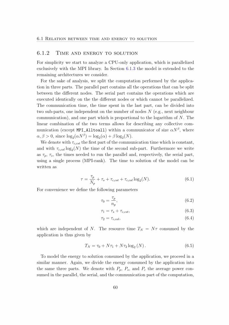
6.1 Relation between time and energy to solution
6.1.2 Time and energy to solution
For simplicity we start to analyze a CPU-only application, which is parallelized
exclusively with the MPI library. In Section 6.1.3 the model is extended to the
remaining architectures we consider.
For the sake of analysis, we split the computation performed by the applica-
tion in three parts. The parallel part contains all the operations that can be split
between the different nodes. The serial part contains the operations which are
executed identically on the the different nodes or which cannot be parallelized.
The communication time, the time spent in the last part, can be divided into
two sub-parts, one independent on the number of nodes N (e.g., next neighbour
communication), and one part which is proportional to the logarithm of N . The
linear combination of the two terms allows for describing any collective com-
munication (except MPI_Alltoall) within a communicator of size αNβ, where
α, β > 0, since log2(αNβ) = log2(α) + β log2(N).
We denote with τc,cst the first part of the communication time which is constant,
and with τc,col log2(N) the time of the second sub-part. Furthermore we write
as τp, τs, the times needed to run the parallel and, respectively, the serial part,
using a single process (MPI-rank). The time to solution of the model can be
written as
τ =τpNp
+ τs + τc,cst + τc,col log2(N). (6.1)
For convenience we define the following parameters
τ0 =τpnp, (6.2)
τ1 = τs + τc,cst, (6.3)
τ2 = τc,col, (6.4)
which are independent of N . The resource time TN = Nτ consumed by the
application is thus given by
TN = τ0 +Nτ1 +Nτ2 log2 (N) . (6.5)
To model the energy to solution consumed by the application, we proceed in a
similar manner. Again, we divide the energy consumed by the application into
the same three parts. We denote with Pp, Ps, and Pc the average power con-
sumed in the parallel, the serial, and the communication part of the computation,
60

Modeling power consumption
respectively. For convenience we also define the constants
P0 = Pp, (6.6)
P1 =1
τ1(Psτs + Pcτc,cst) , (6.7)
P2 = Pc, (6.8)
which are independent of N . The total energy to solution is then
E = P0τ0 +NP1τ1 +NP2τ2 log2 (N) . (6.9)
6.1.3 Model extension
The model presented in the previous section, should be extended to cover multi-
and many-core based node architecture as well as hybrid node architectures, and
their respective node-level parallel decomposition. The multi-core architecture
allows two different node-level decompositions, using a communication library
and a threading library. We again divide the computation into parallel, serial,
and communication parts. In this case, the parallel part can also be divided into
a single and multi-thread part. On the other hand, the serial part is composed of
three sub-parts: a single thread part, a multi-thread part in which each thread
executes the same computations, and a second multi-thread part in which the
threads cooperate to perform the operations in parallel.
We can now redefine the constants of the model, since the decompositions do
not depend on the number of nodes. The parallel time τ0 becomes the sum
of the time spent in the parallel sub-parts on one node, and Pp becomes the
weighted average of the power needed by these sub-parts. Similarly, we redefine
τs as the time needed by the sub-components of the serial part, and Ps as the
weighted average of the power needed by the serial sub-parts. Furthermore, the
two components of communication time depend on the number of MPI-ranks per
node.
The resource time TN and the energy to solution E consumed by the application
remain in the form of Eq. (6.5) and, respectively, Eq. (6.9).
The same procedure can be used to extend the model to the hybrid architecture.
6.1.4 Relating the model to observations
Cumming et al. [38] observed that an affine relationship exists between the
energy to solution and the consumed compute resources (measured in node-
61

6.1 Relation between time and energy to solution
0.2 0.3 0.4 0.5 0.6 0.7 0.8Node hours (h)
0.15
0.20
0.25
0.30
0.35
0.40
0.45Energ
y (
MJ)
Hybrid E. hw, 24, 1 E. hw, 2, 12
Figure 6.1: Energy to solution vs. node-hours for the hybrid and ELPA gener-
alized eigenvalue solvers, solving a problem with matrix size M = 20480. The
same run was executed using different sets of physical nodes for each number of
nodes N , which were also varied.
hours). Specifically they found that
E = π0TN + E0 (6.10)
holds for the regional climate model COSMO and the HPCG benchmark. In
these two codes the global communication is negligible, thus τ2 ≈ 0, hence we
can rewrite our model for energy to solution as
E = P0τ0 +NP1τ1 +NP2τ2 log2 (N)
= (P0 − P1) τ0 + P1TN + (P2 − P1)Nτ2 log2 (N)
≈ (P0 − P1) τ0 + P1TN .
(6.11)
We can thus conclude from the model that the affine relationship between the
energy to solution and the consumed compute resources time holds for any ap-
plication in which the global communication is negligible.
Furthermore, the measurements collected for the generalized eigensolver for
dense, complex, Hermitian matrices shows the same relationship holds, as demon-
strated by the data presented in Fig. 6.1.
62

Modeling power consumption
With this motivation in mind, we want to analyze the relationship between the
resource time and the energy to solution, and compare with its linear regression.
In order to determine how well it fits with this model, we compute the coefficient
of determination r2 of the linear regression.
Since the parallel part only adds a constant term to the resource time and to
the energy to solution, we will neglect it to simplify the next calculations. Let
us then define
Tj = Njτ1 +Njτ2 log2 (Nj) (6.12)
Ej = P1Njτ1 + P2Njτ2 log2 (Nj) , (6.13)
where Nj is the number of nodes used in the j-th measurement, and Tj, Ejare the value of the measurements according to the model. We also define the
following quantities
α =
∑kj=1Nj
2
k−(∑k
j=1Nj
k
)2
(6.14)
β =
∑kj=1Nj
2 log2 (Nj)
k−(∑k
j=1Nj
k
)(∑kj=1Nj log2 (Nj)
k
)(6.15)
γ =
∑kj=1 (Nj log2 (Nj))
2
k−(∑k
j=1Nj log2 (Nj)
k
)2
, (6.16)
where k is the total number of measurements. The value of the fitting parameters
is then given by
π0 =P1τ1
2α + (P1 + P2) τ1τ2β + P2τ22γ
τ12α + 2τ1τ2β + τ22γ(6.17)
E0 = (P1 − π0) τ1∑k
j=1Nj
k+ (P2 − π0) τ2
∑kj=1Nj log2 (Nj)
k, (6.18)
where E0 = E0− (P0 − π0) τ0 due to the shift in the resource time and energy to
solution introduced.
Therefore, the coefficient of indetermination is given by
1− r2 =τ1
2τ22 (P2 − P1)
2 (αγ − β2)
(τ12α + 2τ1τ2β + τ22γ)(P1
2τ12α + 2P1P2τ1τ2β + P22τ22γ
) (6.19)
=:(αγ − β2)
D. (6.20)
63

6.1 Relation between time and energy to solution
k 2 3 4 5 6 7 8 9 10
1− r2 [·10−3] 2.24 2.82 2.75 2.44 2.09 1.77 1.49 1.25 1.06
Table 6.1: Upper bound for the indetermination coefficient 1 − r2 assuming
measurements according to the model using 1, 2, 4, ..., 2k nodes.
The denominator D can be written as
(P2 − P1)2D =
(τ1τ2
)2
P12α2 +
(τ2τ1
)2
P22γ2 + 4P1P2β
2 +(P 21 + P 2
2
)αγ
+ 2(P1
2 + P1P2
) τ1τ2αβ + 2
(P1P2 + P2
2) τ2τ1βγ.
(6.21)
Since we are interested in the upper bound of 1 − r2, the lower bound of the
denominator D has to be found. The minimization over the value of τ1/τ2 gives
D ≥ 2P1P2 (αγ + 2β2) + (P 21 + P 2
2 )αγ + 4 (P1 + P2)√P1P2αγ β
(P2 − P1)2 (6.22)
= αγ +4f
(f − 1)2(αγ + β2
)+ 4
(f + 1)√f
(f − 1)2√αγ β, (6.23)
where f = max(P1, P2)/min(P1, P2) ≥ 1. Assuming that the time to solution and
the energy to solution are measured using 1, 2, 4, ..., 2k nodes, and that f ≤ 10,
the upper bound of the coefficient of indetermination is smaller than 3 · 10−3.
Table 6.1 presents the values for different k. Similarly using 4, 8, 16, ..., 2k nodes
the upper bound of 1− r2 is smaller than 1.3 · 10−3.
We can thus conclude from the model that the affine relationship of the form
of
E = π0TN + E0,
between ETS and consumed compute resources, does not only hold for the appli-
cations in which the global time is negligible, but it also applies approximately
to all the applications which time and energy to solution can be decomposed ac-
cording to the model we presented. This is the case of the eigensolver we study
below, in which τ2 is not small. Furthermore, from Eq. 6.17 it is clear that the
measured parameter π0 is in the range between P1 and P2 and that its precise
interpretation will depend on the application and the system architecture.
64

Modeling power consumption
6.2 Energy measurements
The energy and power measurements presented in this work have been performed
on the Cray XC platform installed at the Swiss National Supercomputing Centre
(CSCS). It is composed by two sub-systems, “Piz Daint” a 28 cabinet Cray XC30
system with 5272 hybrid compute nodes, and “Piz Dora” a 7 cabinet Cray XC40
system with 1256 compute nodes. Each hybrid compute node of the XC30 system
contains an 8-core Intel Xeon E5-2670 CPU and an Nvidia K20x GPGPU. The
compute node of the XC40 system contains two 12-core Intel Xeon E5-2690-v3
CPUs.
The Cray XC platform is ideal for studying energy and power consumption
models, since it is equipped with fine grained power measuring capabilities, as
well as advanced software functionalities that allow the users to extract power
and energy readings for their applications.
Each computing node has a dedicated power sensor, which measures the power
consumed by the entire node, and each hybrid node has an additional sensor
that measures the power consumption of the GPGPU module. The rest of the
components that are located outside the node, i.e., the blowers and the Aries
network, can be measured individually.
The power measurements of the Cray XC platform has been studied and val-
idated by Fourestey et al. [27]. This study finds that the Aries network has a
constant power consumption of 25W per node (100W per blade), and that the
blower power consumption is typically 4400W per blower under normal produc-
tion conditions, but it may have peaks at 5600W per blower when the system
executes exceptionally high loads. “Piz Daint” is equipped with 17 blowers, this
means that the contribution to the power consumption by the blower is about
15 W per node. Hence the difference between the average load and the peak is
of the order of 2W and can be neglected.
Let us denote t as the time to solution and N as the number of nodes used.
Furthermore, Enodes denotes the energy consumed by the compute nodes used
for a simulation. Enodes is the integral over the time of the power measured at
node-level and summed over the N nodes. The total energy to solution can be
calculated fromEnodes + (25 W×N + 4400 W× α) t
0.95, (6.24)
where α is the fraction of blowers contributing to the simulation. The denomi-
nator corresponds to the 95% efficiency for AC/DC conversion [27].
65

6.3 Measurements error
In this work we just consider the energy consumed by the nodes, since we are
only interested in the comparison of different node architectures. In any case,
since the power consumption of the Aries Network per node and the AC-DC
conversion factor are constant, and the power consumption of the blowers is
almost constant, they are not of real interest. Therefore we use
E = Enodes. (6.25)
To determine the energy consumption of the application, the information that
the system stores in cumulative counters can be accessed during the execution.
Each node provides these counters in the form of pm counters files:
- /sys/cray/pm_counters/energy, and
- /sys/cray/pm_counters/accel_energy.
The first counter provides the cumulative energy consumed by the whole compute
node, while the second provides the same information for the GPU module.
6.3 Measurements error
6.3.1 Energy error model
To validate the energy to solution model, we develop an error model to deter-
mine the error of any energy measurement with respect to the measured time to
solution. The energy consumed by the i-th node can be found by integrating the
power consumption, i.e.,
Ei =
∫ t
0
Pi(t′)dt′ ≈ 1
ν
νt∑j=0
Pi(j
ν), (6.26)
where t represents the time to solution and Pi(t′) is the power consumption at
the instant t′. ν represents the update frequency of the energy measurements.
The measured power consumption, Pi, is assumed to differ from the real value
in the following form
Pi(τ) = Pi(τ)(1 + δ1) + δ2 + δ3, (6.27)
where δ1 and δ2 are systematic errors that originate primarily from the calibration
of the sensor, which, by assumption, are constant in time. δ3 represents the
66

Modeling power consumption
statistical error, which we assume is Gauss distributed with standard deviation
σ3. The measured value of the energy consumed by the i-th node then becomes
Ei =1
ν
νt∑j=0
Pi(j
ν) (6.28)
= Ei(1 + δ1) + tδ2 +√tδ3, (6.29)
where δ3 is Gauss distributed with standard deviation σ3 = σ3/√ν. We assume
then that, for the calibration of the sensors, δ1 and δ2 are Gauss distributed with
standard deviation σ1, and σ2, respectively. It follows that the measured total
Energy E for N nodes is
E = E +E√N
∆1 +√N t∆2 +
√Nt∆3. (6.30)
The probability distribution of ∆1, ∆2, and ∆3 are Gauss distributions with
standard deviation σ1, σ2, and σ3, respectively.
6.3.2 Energy error determination
In order to determine the statistical error of the energy measurements, we have to
briefly understand which effects may lead to fluctuations in the time to solution
and in the energy to solution measurements. The first possible variation that
can affect the time to solution, is due to differences in hardware performance,
and contributes to the systematic error. This effect has two origins, on one hand
the simple variation of the node performance, and the position of the nodes
inside the network topology that varies the communication performance. On
the other hand, environmental factors may affect the system performance, e.g.,
communication intensive jobs, running on the system may congest the network
and increase communication time. Those variations contribute to the statistical
error.
To determine the statistical error we have to determine the qualitative origins
of the fluctuations. Since the systematic error depends exclusively on which
nodes are used to execute the job, the statistical error (σ3) can be determined
by executing the same experiment using an identical set of nodes many times.
Fig. 6.2 shows the distribution of the time to solution and energy to solution
measurements. From those measurements we can infer a probability distribution
for σ3.
67

6.3 Measurements error
0.55 0.56 0.57 0.58 0.59Node hours (h)
360
365
370
375
380
385
390
Energ
y (
kJ)
E. hw, 24, 1
Figure 6.2: Energy to solution vs. node-time for the ELPA generalized eigenvalue
solver solving a problem with matrix size M = 20480, using the same set of 64
nodes for each measurement.
To find the probability distribution of σ3, we use Bayes theorem [59] that in
our case states
P (σ3|data, I) ∝ P (data|σ3, I)× P (σ3|I), (6.31)
where data represents the collected measurement and I refers to the background
information.
The prior probability term, P (σ3|I), represents the state of the knowledge
about the validity of the hypothesis on σ3 before the analysis of the data. This
probability is then modified by the likelihood function P (data|σ3, I) generated
from the measurements, and yields the posterior probability P (σ3|data, I) that
represents the state of knowledge after the analysis of the data.
From the energy model 6.10 we know that the measurements lie on the line
given by E = π0T + E0. Hence we can rewrite 6.31 as
P (σ3|data, I) =
∫dπ0
∫dE0P (σ3, π0, E0|data, I) (6.32)
∝∫dπ0
∫dE0P (data|σ3, π0, E0, I)× P (σ3, π0, E0|I). (6.33)
We assume we don’t have any knowledge about the value of the parameters of
the affine fit π0 and E0, hence the prior probability P (π0, E0, σ3|I) = 1 for σ3 > 0
68

Modeling power consumption
and vanishes otherwise. So the posterior probability is given by
P (σ3|data, I) ∝∫ ∞−∞
dπ0
∫ ∞−∞
dE0P (data|σ3, π0, E0, I), (6.34)
for σ3 > 0. The likelihood function is determined using the least-squares method,
hence it becomes
P (data|σ3, π0, E0, I) =∏k
1√2π δ3,k
exp
(−(Ek − εk)2
2δ3,k2
), (6.35)
where Ek and Tk are the k-th measurement of the energy to solution, respectively
of the time to solution, εk = π0Tk + E0 and δ3,k = σ3√Tk.
Defining δk := δ3,k, the posterior probability evaluates to
P (σ3|data, I) ∝ P (data|σ3, I)× P (σ3|I), (6.36)
where
P (data|σ3, I) :=
(∏k
1
δk
)∆√C2
exp
(−1
2
(C0 −
C12
C2
)), (6.37)
and the prior probability P (σ3|I) = 1 for σ3 > 0 and vanishes otherwise. The
coefficients are defined as
1
∆2=∑k
1
δk2 ,
C0 =∑k
(Ekδk
)2
−(∑
k
Ek
δk2
)2
∆2,
C1 =∑k
(EkTk
δk2
)−(∑
k
Tk
δk2
)(∑k
Ek
δk2
)∆2,
C2 =∑k
(Tkδk
)2
−(∑
k
Tk
δk2
)2
∆2.
(6.38)
Using δk = σ3√Nt the result simplifies to
P (σ3|data, I) ∝ σ32−m exp
(− 1
2σ32C3
), (6.39)
for σ3 > 0, where m is the number of measurements and C3 = σ32(C0−C1
2/C2)
is constant with respect to σ3.
69

6.3 Measurements error
The posterior probability can now be approximated with the Gauss distribu-
tion, yielding
σ3 =
√C3
m− 2
(1±
√1
2(m− 2)
). (6.40)
Fig. 6.3 and Fig. 6.4 show the comparison between the posterior probability
for σ3 and its Gauss approximation.
The second type of error that has to be determined is the systematic error.
This type of error depends on the position of the nodes in the network topol-
ogy. To estimate its value, the same problem is executed several times using
different nodes (different number of nodes and different physical nodes). These
measurements are denoted with data, and, when integrating the systematic error
in Eq. 6.33 we get
P (σ1, σ2, σ3|data, I) =
∫dπ0
∫dE0P (σ1, σ2, σ3, π0, E0|data, I) (6.41)
∝∫dπ0
∫dE0
(P (data|σ1, σ2, σ3, π0, E0, I)
× P (σ1, σ2, σ3, π0, E0|I)).
(6.42)
We define, for convenience
ck =1
√2π
3δ1,kδ2,kδ3,k
. (6.43)
The likelihood function becomes
P (data|σ1, σ2, σ3, π0, E0, I) (6.44)
=∏k
∫de1
∫de2 ck exp
(− e1
2
2δ1,k2 −
e22
2δ2,k2 −
(Ek − εk − e1 − e2)22δ3,k
2
)(6.45)
=∏k
1√2π δk
exp
(−(Ek − εk)2
2δk2
), (6.46)
where Ek and Tk are the k-th measurement of the energy to solution, respectively,
of the time to solution, εk = π0Tk + E0, δ1,k = σ1Ek/√N , δ2,k = σ2Tk/
√N ,
δ3,k = σ3√Tk. δk :=
√δ1,k
2 + δ2,k2 + δ3,k
2 represent the size of the error of the
measurement Ek. The likelihood function has the same form as in the statistical
error calculation. Assuming we don’t have any knowledge about the value of π0and E0, the posterior probability evaluates to
P (σ1, σ2, σ3|data, I) ∝ P (data|σ1, σ2, σ3, I)× P (σ1, σ2, σ3|I), (6.47)
70

Modeling power consumption
0.55 0.56 0.57 0.58 0.59Node hours (h)
360
365
370
375
380
385
390
Energ
y (
kJ)
E. hw, 24, 1
18 20 22 24 26 28σ3 [W
√s ]
0.00
0.05
0.10
0.15
0.20
0.25
0.30
0.35
0.40Prob. distr. Gauss approx.
Figure 6.3: Left: Energy to solution vs. node-time for the ELPA generalized
eigenvalue solver solving a problem with matrix size M = 20480. The same set of
64 nodes was used for all the measurements. Right: The probability distribution
found for the value of σ3 and its Gaussian approximation.
0.310 0.315 0.320 0.325Node hours (h)
175
176
177
178
179
180
181
182
Energ
y (
kJ)
Hybrid
11 12 13 14 15 16 17 18σ3 [W
√s ]
0.0
0.1
0.2
0.3
0.4
0.5
0.6Prob. distr. Gauss approx.
Figure 6.4: Left: Energy to solution vs. node-time for the hybrid generalized
eigenvalue solver solving a problem with matrix size M = 20480. The same set of
16 nodes was used for all the measurements. Right: The probability distribution
found for the value of σ3 and its Gaussian approximation.
71
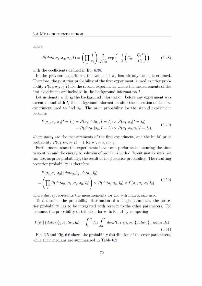
6.3 Measurements error
where
P (data|σ1, σ2, σ3, I) =
(∏k
1
δk
)∆√C2
exp
(−1
2
(C0 −
C12
C2
)), (6.48)
with the coefficients defined in Eq. 6.38.
In the previous experiment the value for σ3 has already been determined.
Therefore, the posterior probability of the first experiment is used as prior prob-
ability P (σ1, σ2, σ3|I) for the second experiment, where the measurements of the
first experiment are included in the background information I.
Let us denote with I0 the background information, before any experiment was
executed, and with I1 the background information after the execution of the first
experiment used to find σ3. The prior probability for the second experiment
becomes
P (σ1, σ2, σ3|I = I1) = P (σ3|data1, I = I0)× P (σ1, σ2|I = I0)
= P (data1|σ3, I = I0)× P (σ1, σ2, σ3|I = I0),(6.49)
where data1 are the measurements of the first experiment, and the initial prior
probability P (σ1, σ2, σ3|I) = 1 for σ1, σ2, σ3 > 0.
Furthermore, since the experiments have been performed measuring the time
to solution and the energy to solution of problems with different matrix sizes, we
can use, as prior probability, the result of the posterior probability. The resulting
posterior probability is therefore
P (σ1, σ2, σ3| {data2,i}i , data1, I0)
=
(∏i
P (data2,i|σ1, σ2, σ3, I0))× P (data1|σ3, I0)× P (σ1, σ2, σ3|I0),
(6.50)
where data2,i represents the measurements for the i-th matrix size used.
To determine the probability distribution of a single parameter, the poste-
rior probability has to be integrated with respect to the other parameters. For
instance, the probability distribution for σ1 is found by computing
P (σ1| {data2,i}i , data1, I0) =
∫ ∞0
dσ2
∫ ∞0
dσ3P (σ1, σ2, σ3| {data2,i}i , data1, I0)(6.51)
Fig. 6.5 and Fig. 6.6 shows the probability distribution of the error parameters,
while their medians are summarized in Table 6.2
72

Modeling power consumption
0.0 0.5 1.0 1.5 2.0 2.5 3.0 3.5 4.0
σ1 [10−2 ]
0.0
0.1
0.2
0.3
0.4
0.5
3 4 5 6 7 8 9σ2 [W]
0.0
0.2
0.4
0.6
0.8
1.0
1.2
18 20 22 24 26 28 30σ3 [W
√s ]
0.00
0.05
0.10
0.15
0.20
0.25
0.30
0.35
0.40
Figure 6.5: Probability distribution of the error parameters found for ELPA
executed on Piz Dora. The vertical line represents the median of the probability
distribution.
σ1 σ2 [W] σ3 [W√
s]
Piz Dora 0.011 7.30 24.2
Piz Daint (2 CPUs) 0.009 13.5 37.4
Piz Daint Hybrid 0.011 3.66 14.5
Piz Daint Hybrid (CPU) 0.069 1.05 12.5
Piz Daint Hybrid (GPU) 0.040 3.05 6.80
Table 6.2: The values of the standard deviation of the distribution of the different
the errors for different systems.
73

6.3 Measurements error
0.0 0.5 1.0 1.5 2.0 2.5 3.0
σ1 [10−2 ]
0.0
0.1
0.2
0.3
0.4
0.5
0.6
0.7
2.0 2.5 3.0 3.5 4.0 4.5 5.0σ2 [W]
0.0
0.2
0.4
0.6
0.8
1.0
1.2
1.4
10 11 12 13 14 15 16 17 18 19σ3 [W
√s ]
0.0
0.1
0.2
0.3
0.4
0.5
0.6
Figure 6.6: Probability distribution of the error parameters found for the hybrid
solver executed on Piz Daint. The vertical line represents the median of the
probability distribution.
74

Modeling power consumption
We can see that the values for Piz Daint and Piz Dora agree. In fact, for
Piz Daint we have twice the number of sensors, since we simulate a dual-socket
multi-core CPU node using two single-socket nodes neglecting the GPU. Hence
σ1 is around a factor√
2 smaller, while σ3 is around a factor√
2 larger. σ2 is
more than a factor√
2 larger, since the idle GPU and its sensor add an extra
source of error that is constant during the execution.
6.4 Energy results
To validate the energy to solution model we benchmark the distributed hybrid
CPU-GPU solver presented in Chapter 5 and the ELPA2 generalized eigenvalue
solver presented in Section 1.2.
The results presented in this section were produced fixing the P state of the
CPU governor to the nominal frequency of the CPU (2.6 GHz for both the Intel
Xeon E5-2670 of the Cray XC30 and the Intel Xeon E5-2690-v3 of the Cray
XC40) for the runs with ELPA. This means that we disabled the Turbo Boost
of the CPUs.
Moreover, when running CPU-only algorithms (in this case ELPA2) on the
hybrid Cray XC30 system a, “node” is considered to be a set of two physical
nodes, since we want a comparison of systems using two sockets per nodes. The
power consumption of the idle GPU is, in this case, subtracted from the total
power consumption of the node in the reported results.
The ELPA solver is implemented using both MPI libraries for the inter-process
communication and the OpenMP programming model intra-process parallelism.
Therefore, it is capable of running different combinations of MPI processes per
node and OpenMP threads per process on the same number of nodes, as discussed
in section 6.1.1.
Fig. 6.7 and Fig. 6.8 present the weak scaling of the time and the energy to
solution of the solvers. These results are similar to the results presented in 5.4.1;
the only difference is that the Turbo Boost of the Intel CPUs was disabled for
the ELPA runs. The algorithmic complexity of the generalized eigensolver is
O(M3), where M is the matrix size, therefore the weak scaling of the energy to
solution is proportional to M3. On the other hand, since the number of nodes
N used is proportional to M2, the perfect weak scaling of the time to solution is
proportional to M . As expected, the results show a deviation from the perfect
scaling.
The strong scaling of the time and energy to solution for a problem of matrix
75

6.4 Energy results
20 40 60 80 100Matrix size M [×1000]
1.0
1.5
2.0
2.5
3.0
3.5
4.0
4.5
t/M
norm
aliz
ed
Hybrid
E. sb, 16, 1
E. sb, 8, 2
E. sb, 4, 4
E. sb, 2, 8
E. hw, 24, 1
E. hw, 12, 2
E. hw, 6, 4
E. hw, 4, 6
E. hw, 2, 12
Figure 6.7: Weak scaling of time to solution on Piz Daint and Piz Dora of the
hybrid and ELPA generalized eigenvalue solvers, using (M/10240)2 nodes. The
results are normalized to the value of the hybrid solver solving a problem with
matrix size M = 10240.
20 40 60 80 100Matrix size M [×1000]
1.0
1.5
2.0
2.5
3.0
3.5
4.0
4.5
E/M
3 n
orm
aliz
ed
Hybrid
E. sb, 16, 1
E. sb, 8, 2
E. sb, 4, 4
E. sb, 2, 8
E. hw, 24, 1
E. hw, 12, 2
E. hw, 6, 4
E. hw, 4, 6
E. hw, 2, 12
Figure 6.8: Weak scaling of energy to solution on Piz Daint and Piz Dora of the
hybrid and ELPA generalized eigenvalue solvers, using (M/10240)2 nodes. The
results are normalized to the value of the hybrid solver solving a problem with
matrix size M = 10240.
76

Modeling power consumption
6 12 25 50 100 200 400Number of nodes N
102
103
Tim
e [
s]
6 12 25 50 100 200 400Number of nodes N
100
101
Energ
y [
MJ]
Hybrid
E. sb, 16, 1
E. sb, 8, 2
E. sb, 4, 4
E. sb, 2, 8
Figure 6.9: Strong scaling of the time and the energy to solution for the hybrid
and ELPA generalized eigenvalue solvers, solving a problem with matrix size
M = 51200.
6 12 25 50 100 200 400Number of nodes N
102
103
Tim
e [
s]
6 12 25 50 100 200 400Number of nodes N
100
101
Energ
y [
MJ]
E. hw, 24, 1
E. hw, 12, 2
E. hw, 6, 4
E. hw, 4, 6
E. hw, 2, 12
Figure 6.10: Strong scaling of the time and the energy to solution for the hybrid
and ELPA generalized eigenvalue solvers, solving a problem with matrix size
M = 51200.
77

6.4 Energy results
4 6 8 10 12 14 16 18Node hours (h)
2
4
6
8
10
12
14
Energ
y (
MJ)
Hybrid
E. sb, 16, 1
E. sb, 8, 2
E. sb, 4, 4
E. sb, 2, 8
Figure 6.11: ETS vs. node-hours on Piz Daint for the hybrid and ELPA gener-
alized eigenvalue solvers, solving a problem with matrix size M = 51200. The
results show an affine relationship between the two quantities. The solid line
represents the affine fit.
78

Modeling power consumption
4 6 8 10 12Node hours (h)
3
4
5
6
7
8
Energ
y (
MJ)
E. hw, 24, 1
E. hw, 12, 2
E. hw, 6, 4
E. hw, 4, 6
E. hw, 2, 12
Figure 6.12: ETS vs. node-hours on Piz Dora for the ELPA generalized eigen-
value solver, solving a problem with matrix size 51200 and computing all the
eigenvectors. The solid line represents the affine fit.
79

6.4 Energy results
Type np nt π0 [W] E0 [MJ] 1− r2Hybrid 1 8 114.9± 0.4 0.91± 0.01 6.5 · 10−6
E. sb 16 1 213.5± 2.2 1.17± 0.08 1.24 · 10−3
E. sb 8 2 199.5± 1.7 1.56± 0.07 9.6 · 10−4
E. sb 4 4 187.6± 2.0 1.80± 0.09 5.7 · 10−4
E. sb 2 8 184.8± 1.8 1.78± 0.08 1.27 · 10−3
E. hw 24 1 162.3± 1.3 0.68± 0.03 5.4 · 10−4
E. hw 12 2 139.9± 1.5 1.10± 0.04 4.4 · 10−4
E. hw 6 4 130.4± 1.6 1.20± 0.04 1.63 · 10−3
E. hw 4 6 129.5± 1.8 1.19± 0.04 1.52 · 10−3
E. hw 2 12 131.0± 1.7 1.09± 0.05 6.5 · 10−4
Table 6.3: Values of the fit parameters π0 and E0 of the results of hybrid and the
ELPA generalized eigenvalue solver, for a problem with matrix size M = 51200.
The results are shown in Fig. 6.11 and 6.12
size M = 51200 are presented in Fig. 6.9 and Fig. 6.10. Using the data collected
for the strong scaling plots, we built a diagram which shows the relationship
between the resource time and the energy to solution. Fig. 6.11 and Fig. 6.12
show the existence of an affine relationship between the node-hour and the energy
to solution. For each set of data included in Fig. 6.11 and Fig. 6.12, we checked
the quality of the affine fit, computing the coefficient of indetermination 1− r2,which is listed in Table 6.3. The values of the coefficient show that the quality of
the affine fits are good. Table 6.3 also presents the value of the parameters π0 and
E0 which fit the measurements. The evaluation of error bars of the measurements
is performed using the results shown in section 6.3.
The affine behaviour has been analyzed for different matrix sizes M , and the fit
parameters π0 and E0 have been computed for each size. Fig. 6.13 and Fig. 6.14
show the values of π0 and ε0 := E0/M3 for different matrix sizes and different
node configurations. For a given node architecture and intra-node parallelism,
π0 and ε0 show a constant behaviour within the errorbars. This is remarkable,
since E0 reflects the complexity of the underlying algorithm even if the data
were extracted from parallel runs at scale which do not have perfect parallel
efficiency. Therefore E0 can indeed be interpreted as the dynamic energy of the
bare computation [38]. On the other hand, the parameter π0 can be interpreted
as the static contribution for all the parts of the computation which do not scale
or in which the system is idle. It is clear that the the value of π0 increases when
80

Modeling power consumption
Type np nt π0 [W] ε0 [nJ]
Hybrid 1 8 115.5± 0.1 6.63± 0.02
E. sb 16 1 214.5± 0.9 8.59± 0.25
E. sb 8 2 201.7± 0.7 10.90± 0.22
E. sb 4 4 188.7± 0.7 12.91± 0.23
E. sb 2 8 182.0± 0.8 13.94± 0.24
E. hw 24 1 161.3± 0.5 5.32± 0.11
E. hw 12 2 140.0± 0.5 8.16± 0.11
E. hw 6 4 129.1± 0.6 9.09± 0.12
E. hw 4 6 128.8± 0.7 8.94± 0.14
E. hw 2 12 128.4± 0.6 8.71± 0.15
Table 6.4: Values of the averages of π0 and ε0 := E0/M3 for the hybrid and the
ELPA generalized eigenvalue solver, found in Fig. 6.14 and Fig. 6.13
the number of MPI ranks per node increase. This fact is related to the MPI
implementation, specifically to the operation executed when a process is waiting
for a message. This behaviour is further investigated in Section 6.5.
The average values of π0 and ε0 found for the different configurations are listed
in Table 6.4. From these values it is possible to predict the energy to solution of
the generalized eigensolver from the measured time to solution, the number of
nodes used, and the matrix size.
Using the value given in Table 6.4, we compute the energy to solution from
Eq. (6.10) from the time to solution measurements, and we can compare these
with the energy measurements. On one hand we can compare the the computed
values for the time to solution depicted in Fig. 6.7 with the measured value
depicted in Fig. 6.8. As expected, the comparison in Fig. 6.15 shows that the
predicted energies agree with the measurements within the error bar.
On the other hand we can also compare the measured value of the energy to
solution shown in Fig. 6.11 with the model predicted values. Even if the value of
the fit parameters π0 and E0 are not close to the average value (see values with
M = 51200 in Fig. 6.13a and Fig. 6.14a), the comparison in Fig. 6.16 shows a
good agreement of the measurements and the model predicted values within the
error bar.
We also applied the same procedure to measurements of the generalized eigen-
solvers, computing only 50% of the eigenvectors. Fig. 6.17 and Fig. 6.18 show
the values of π0 and ε0, and their average values found for the different configu-
81

6.4 Energy results
0 20 40 60 80 100Matrix size M [×1000]
10
12
14
16
18
20
22
π0 [×1
0 W
]
Hybrid
E. sb, 16, 1
E. sb, 8, 2
E. sb, 4, 4
E. sb, 2, 8
(a) Piz Daint
0 20 40 60 80 100Matrix size M [×1000]
10
12
14
16
18
20
22
π0 [×1
0 W
]
E. hw, 24, 1
E. hw, 12, 2
E. hw, 6, 4
E. hw, 4, 6
E. hw, 2, 12
(b) Piz Dora
Figure 6.13: Values of π0 of the hybrid and the ELPA generalized eigenvalue
solver.
0 20 40 60 80 100Matrix size M [×1000]
0.5
1.0
1.5
2.0
2.5
3.0
3.5
E0/M
3 n
orm
aliz
ed
Hybrid
E. sb, 16, 1
E. sb, 8, 2
E. sb, 4, 4
E. sb, 2, 8
(a) Piz Daint
0 20 40 60 80 100Matrix size M [×1000]
0.5
1.0
1.5
2.0
2.5
3.0
3.5
E0/M
3 n
orm
aliz
ed
E. hw, 24, 1
E. hw, 12, 2
E. hw, 6, 4
E. hw, 4, 6
E. hw, 2, 12
(b) Piz Dora
Figure 6.14: Values of ε0 of the hybrid and the ELPA generalized eigenvalue
solver, normalized to the value for the hybrid solver solving a 10240 size matrix.
82

Modeling power consumption
20 40 60 80 100Matrix size M [×1000]
1.0
1.5
2.0
2.5
3.0
3.5
4.0
4.5
E/M
3 n
orm
aliz
ed
Hybrid
E. sb, 16, 1
E. sb, 8, 2
E. sb, 4, 4
E. sb, 2, 8
E. hw, 24, 1
E. hw, 12, 2
E. hw, 6, 4
E. hw, 4, 6
E. hw, 2, 12
Model
Figure 6.15: Weak scaling of energy to solution on Piz Daint and Piz Dora of
the hybrid and of ELPA generalized eigenvalue solver, using (M/10240)2 nodes.
The values are normalized to the value of the hybrid solver solving a problem
with M = 10240. The model predictions using the parameters from Table 6.4
(black) are compared with measurements (colored).
83

6.4 Energy results
4 6 8 10 12 14 16 18Node hours (h)
2
4
6
8
10
12
14
Energ
y (
MJ)
Hybrid
E. sb, 16, 1
E. sb, 8, 2
E. sb, 4, 4
E. sb, 2, 8
Figure 6.16: ETS vs. node-hours on Piz Daint for the hybrid and for ELPA
generalized eigenvalue solver, solving a problem with matrix size M = 51200.
The results show an affine relationship between the two quantities. The solid
line represents the model predicted energy to solution.
84

Modeling power consumption
Type np nt π0 [W] ε0 [nJ]
Hybrid 1 8 116.2± 0.1 4.27± 0.02
E. sb 16 1 215.9± 0.9 5.47± 0.20
E. sb 8 2 199.8± 0.7 7.61± 0.15
E. sb 4 4 189.1± 0.8 8.56± 0.20
E. sb 2 8 183.6± 0.7 8.84± 0.17
E. hw 24 1 160.5± 0.4 3.69± 0.07
E. hw 12 2 142.3± 0.5 5.14± 0.07
E. hw 6 4 133.5± 0.5 5.42± 0.08
E. hw 4 6 131.7± 0.5 5.49± 0.09
E. hw 2 12 129.9± 0.5 5.57± 0.09
Table 6.5: Values of the averages of π0 and ε0 := E0/M3 for the hybrid and the
ELPA generalized eigenvalue solver computing 50% of the eigenvectors, found
in Fig. 6.18 and Fig. 6.17
rations are listed in Table 6.5. As expected ,the value of π0 does not have large
variations compared to the previous results, since there is only a small variation
in the power constants P0, P1, and P2 defined in Section 6.1.2. On the other
hand the value of ε0 is smaller since the complexity of the algorithm is reduced.
The same approach used to analyze the total energy to solution can be used
to independently analyze the energy used by the CPU and by the GPU during
a hybrid run.
Fig. 6.19 shows that even for the GPU-only part and the CPU-only part of an
affine relationship exists between the node-hour and the energy to solution. The
coefficient of indetermination 1 − r2 shows that the quality of the affine fit is
good. The values are presented in Table 6.6 as well as the parameters π0 and E0,
which fit the measurements. As expected, the results show that the GPU has a
large dynamic power consumption, since the main computation is done by the
accelerator. On the other hand, the CPU has a larger static power consumption.
The fit parameters π0 and E0 have been computed for each size, and Fig. 6.20
and Fig. 6.21 show the values of π0 and ε0 := E0/M3 for different matrix sizes,
computing either all or 20% of the eigenvectors. π0 and shows a constant be-
haviour within the errorbars. For the energy measurements of the GPU, E0
reflects the complexity of the underlying algorithm. The CPU energy measure-
ments show a constant behaviour of ε0 when computing all the eigenvectors, while
it shows a decaying behaviour when computing only 20% of the eigenvectors.
85

6.4 Energy results
0 20 40 60 80 100Matrix size M [×1000]
10
12
14
16
18
20
22
π0 [×1
0 W
]
Hybrid
E. sb, 16, 1
E. sb, 8, 2
E. sb, 4, 4
E. sb, 2, 8
(a) Piz Daint
0 20 40 60 80 100Matrix size M [×1000]
10
12
14
16
18
20
22
π0 [×1
0 W
]
E. hw, 24, 1
E. hw, 12, 2
E. hw, 6, 4
E. hw, 4, 6
E. hw, 2, 12
(b) Piz Dora
Figure 6.17: Values of π0 of the hybrid and the ELPA generalized eigenvalue
solver computing 50% of the eigenvectors.
0 20 40 60 80 100Matrix size M [×1000]
0.5
1.0
1.5
2.0
2.5
3.0
3.5
E0/M
3 n
orm
aliz
ed
Hybrid
E. sb, 16, 1
E. sb, 8, 2
E. sb, 4, 4
E. sb, 2, 8
(a) Piz Daint
0 20 40 60 80 100Matrix size M [×1000]
0.5
1.0
1.5
2.0
2.5
3.0
3.5
E0/M
3 n
orm
aliz
ed
E. hw, 24, 1
E. hw, 12, 2
E. hw, 6, 4
E. hw, 4, 6
E. hw, 2, 12
(b) Piz Dora
Figure 6.18: Values of ε0 of the hybrid and the ELPA generalized eigenvalue
solver computing 50% of the eigenvectors, normalized to the value for the hybrid
solver solving a 10240 size matrix.
86

Modeling power consumption
4 6 8 10 12 14 16Node hours (h)
1
2
3
4
5
6
7
8Energ
y (
MJ)
Hybrid Hybrid CPU Hybrid GPU
Figure 6.19: ETS vs. node-hours on Piz Daint for the hybrid generalized eigen-
value solver, solving a problem with matrix size M = 51200. The results show
an affine relationship between the two quantities. The solid line represents the
affine fit.
Type π0 [W] E0 [kJ] 1− r2Hybrid 114.9± 0.5 913± 13 6.5 · 10−6
Hybrid GPU 46.7± 0.5 819± 14 9.8 · 10−5
Hybrid CPU 68.2± 0.5 92± 14 9.8 · 10−5
Table 6.6: Values of the fit parameters π0 and E0 of the results of the hybrid
solver, for a problem with matrix size M = 51200. The results are shown in
Fig. 6.19.
87

6.4 Energy results
100% Eigenvectors 20% Eigenvectors
M E0 total [kJ] E0 back Q1 [kJ] E0 total [kJ] E0 back Q1 [kJ]
10240 0.91± 0.45 0.39± 0.16 0.68± 0.30 0.103± 0.044
20480 8.3± 2.2 4.7± 1.2 4.5± 1.2 0.79± 0.22
30720 21.0± 4.6 12.7± 2.0 10.0± 2.8 2.42± 0.60
40960 50.4± 8.3 32.6± 3.6 25.9± 4.8 6.34± 0.81
51200 92± 14 64.9± 5.8 48± 8.2 10.3± 1.8
61440 165± 20 107± 10 80± 12 19.0± 2.3
71680 273± 27 182± 11 116± 16 27.0± 3.3
81920 415± 35 276± 16 118± 21 31.3± 4.2
92160 546± 50 386± 25 244± 30 51.3± 7.7
102400 737± 60 498± 30 324± 37 66.7± 8.6
Table 6.7: Values of the fit parameter E0 of the measurements for the CPU of
the full hybrid solver (total) and of the back-transformation with the matrix Q1
(back Q1), for a problem with matrix size M , computing either all or 20% of
the eigenvectors.
Since the complexity of the part of the algorithm executed on the CPU is
O(M2), we expect the value of ε0 for the CPU to have a linear decaying behaviour.
A further analysis of the energy measurements (100% Eigenvectors) shows that
the back-transformation with the matrix Q1 contributes most (∼ 65%) to E0 for
the CPU and shows a O(M3) behaviour. On the other hand, when only 20%
of the eigenvectors are computed, this back-transformation contributes to only
∼ 20% to the values of E0 for the CPU. The value of E0 of the full eigensolver
and for the back-transformation are presented in Table 6.7 for different matrix
sizes.
The back-transformation with the matrix Q1 consists by two phases. The first
phase includes the computation of the T matrix of the compact WY represen-
tation of a householder reflector block with a O(M2) operation executed by the
CPU. The second phase consist of the application of the Householder transforma-
tions, which are O(M3) operations, executed with libsci acc routines and depends
on the number of eigenvectors computed. Therefore the O(M3) contribution of
the CPU is given by the libsci acc routines, which requires further analysis to
determine the exact type of contribution of the CPU.
88

Modeling power consumption
0 20 40 60 80 100Matrix size M [×1000]
0
2
4
6
8
10
12
π0 [×1
0 W
]
Hybrid
Hybrid CPU
Hybrid GPU
(a) 100% Eigenvectors
0 20 40 60 80 100Matrix size M [×1000]
0
2
4
6
8
10
12
π0 [×1
0 W
]
Hybrid
Hybrid CPU
Hybrid GPU
(b) 20% Eigenvectors
Figure 6.20: Values of π0 of the hybrid generalized eigenvalue solver.
0 20 40 60 80 100Matrix size M [×1000]
0.0
0.2
0.4
0.6
0.8
1.0
1.2
E0/M
3 n
orm
aliz
ed
Hybrid
Hybrid CPU
Hybrid GPU
(a) 100% Eigenvectors
0 20 40 60 80 100Matrix size M [×1000]
0.0
0.2
0.4
0.6
0.8
1.0
1.2
E0/M
3 n
orm
aliz
ed
Hybrid
Hybrid CPU
Hybrid GPU
(b) 20% Eigenvectors
Figure 6.21: Values of ε0 of the hybrid eigenvalue solver, normalized to the value
for the hybrid solver solving a 10240 size matrix.
89

6.5 A further power experiment
6.5 A further power experiment
In the previous section, different value of π0 has been found for different parallel
decompositions on the multi-core architecture. We designed an experiment to
investigate the power consumption of the MPI library implementation available
on the Cray XC platform (Cray MPICH) to investigate the reason for this be-
haviour. Therefore, we measure the power consumption for some different ways
to receive an MPI message, and we compare the measurement with the idle power
consumption and the power consumption executing a compute-intensive opera-
tion, varying the number of MPI processes per CPU socket np and the number
of threads per process ntThe experiment has been performed on 4000 nodes of Piz Daint and 800 nodes
on Piz Dora. In both cases the experiment was executed the first time using the
default P state of the CPU governor, which allows a small increase of the oper-
ating frequency due to the Turbo Boost, and the second time setting the P state
to 2.6 GHz. The analysis of the measurements performed on Piz Daint showed
that 4 nodes had a defective GPU power sensor. Therefore this experiment can
be used to diagnose the functionality of the power sensors during operation.
The experiment has been designed to measure the average power consumption
per node for the following six different cases:
1. the MPI processes sleep for 20s;
2. the threads sleep for 20s and execute a blocking receive;
3. the threads execute a blocking receive;
4. the threads execute a non-blocking receive, sleep for 20s, and wait for the
completion of the receive;
5. the threads execute a non-blocking receive and wait for the completion of
the receive;
6. the MPI processes execute a multi-threaded matrix-matrix multiplication
(DGEMM).
The threads which send the MPI message are executed on a different node and
their power consumption is not measured. They sleep for 20s and then send a
40kB message, for the cases in which communication occurs. Case 1 and Case 6
serve as a reference for a fully idle and fully active socket, respectively.
90

Modeling power consumption
20 30 40 50Power (W)
0
200
400
600
Case 1:
20 30 40 50Power (W)
0
200
400
600
800
1000
1200Case 2:
100 110 120Power (W)
0
100
200
300
400
Case 3:
20 30 40 50Power (W)
0
200
400
600
800Case 4:
100 110 120Power (W)
0
100
200
300
400
Case 5:
110 120 130 140Power (W)
0
100
200
300Case 6:
Figure 6.22: Distribution of the CPU power consumption for the 6 cases on Piz
Daint, using np = 8 processes per socket and nt = 1 threads per process. The P
state of the CPU governor is set to 2.6 GHz
91
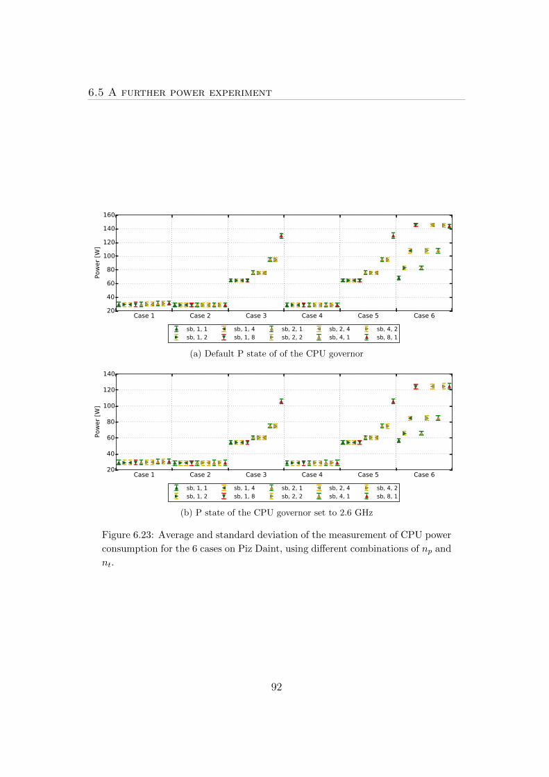
6.5 A further power experiment
Case 1 Case 2 Case 3 Case 4 Case 5 Case 620
40
60
80
100
120
140
160
Pow
er
[W]
sb, 1, 1
sb, 1, 2
sb, 1, 4
sb, 1, 8
sb, 2, 1
sb, 2, 2
sb, 2, 4
sb, 4, 1
sb, 4, 2
sb, 8, 1
(a) Default P state of of the CPU governor
Case 1 Case 2 Case 3 Case 4 Case 5 Case 620
40
60
80
100
120
140
Pow
er
[W]
sb, 1, 1
sb, 1, 2
sb, 1, 4
sb, 1, 8
sb, 2, 1
sb, 2, 2
sb, 2, 4
sb, 4, 1
sb, 4, 2
sb, 8, 1
(b) P state of the CPU governor set to 2.6 GHz
Figure 6.23: Average and standard deviation of the measurement of CPU power
consumption for the 6 cases on Piz Daint, using different combinations of np and
nt.
92

Modeling power consumption
Case 1 Case 2 Case 3 Case 4 Case 5 Case 60
50
100
150
200
250
300
350
400
Pow
er
[W]
sb, 2, 1
sb, 2, 2
sb, 2, 6
sb, 2, 12
sb, 4, 1
sb, 4, 2
sb, 4, 6
sb, 12, 1
sb, 12, 2
sb, 24, 1
(a) Default P state of of the CPU governor
Case 1 Case 2 Case 3 Case 4 Case 5 Case 60
50
100
150
200
250
300
350
Pow
er
[W]
sb, 2, 1
sb, 2, 2
sb, 2, 6
sb, 2, 12
sb, 4, 1
sb, 4, 2
sb, 4, 6
sb, 12, 1
sb, 12, 2
sb, 24, 1
(b) P state of the CPU governor set to 2.6 GHz
Figure 6.24: Average and standard deviation of the measurement of CPU power
consumption for the 6 cases on Piz Dora, using different combinations of np and
nt.
93

6.5 A further power experiment
Fig. 6.22 shows the distribution of the average power measurements for all
six cases, using 8 MPI process per node on Piz Daint. The distributions of the
measurements might be considered to be single Gaussian when the processor is
under compute intensive load, but in reality is a superposition of more Gauss
distributions, in the other cases. This variation of the power consumption may
indicate that the processors and the power sensors are produced in different
batches which have very small differences in the production parameters.
The average and the standard deviation of the power measurements performed
with different parameters np and nt, for the Cray XC30 and the Cray XC40
systems are presented in Fig. 6.23 and 6.24. As expected the difference between
case 1 and cases 2 and 4 is small, since the processors are sleeping for most of the
time. However, it clearly emerges that in cases 3 and 5 the power consumption
increases when a larger number of task per node np is used. Moreover the power
consumption when np is large is not small as showed by the comparison with
case 6, where the processor executes compute intensive operation. Therefore the
processes remain busy during the blocking receive and the blocking wait. On the
other hand, the power consumption does not vary substantially when the number
of threads per task nt increases. These results explain the different values of π0found for the different intra-node parallel decomposition of the eigensolver.
The behaviour found for case 3 and case 5 depends on the MPI implementation,
and can be explained in the following way. For a single-thread application,
MPI uses a loop, which keeps the CPU occupied (busy-waiting) to check the
completion of the reception of a message. In a multi-thread application the MPI
resources cannot be accessed by multiple threads at the same time, hence the
access has to be serialized. In this way, just one thread, the one accessing the
MPI resources, is doing a busy wait, while the other threads use a non-busy wait
mechanism.
This detail can explain the behaviour of the power measurements we found
in the experiment. If the MPI implementation and the network interface sup-
ports non-busy waiting, the latency of the communication can increase, but, the
average power consumption decreases. Therefore, the static power consuption
π0 decreases, and, depending on the application, this could reduce the overall
energy to solution of a parallel run.
94

Chapter 7
Conclusions
In the first part of this thesis we presented the implementation of the generalized
Hermitian positive definite eigenvalue solver. As starting point for the distributed
implementation of the eigensolver we first developed a single-node single-GPU
hybrid implementation, using both the memory bound one-stage algorithm, and
the two-stage compute-bound algorithm. We demonstrated that both the one-
and the two-stage hybrid CPU-GPU implementation of the standard eigensolver,
using a CPU socket and one GPU, show a significant speed-up compared to the
state-of-art CPU-only implementations for shared and distributed memory ar-
chitecture, using two CPU sockets. The same results were observed for the
generalized eigenvalue solver. The results also showed that the two-stage ap-
proach has better performance compared to the one-stage approach, especially
when only a fraction of the eigenvectors has to be computed.
We presented the first parallel approach of the implementation of the eigen-
solver for the single-node multi-GPU architecture. The multi-GPU implementa-
tion of the two-stage solver showed good performance and scalability, as well as a
good speed-up compare to the distributed memory CPU-only implementations.
The multi-GPU implementation demonstrates the possibility to develop efficient
and scalable algorithms for hybrid systems, the components of which have a very
large computing performance compared to the interconnection bandwidth.
We presented the hybrid CPU-GPU distributed memory implementation of the
generalized eigenvalue solver based on the two-stage approach. We compared the
the time to solution and the energy to solution of the hybrid implementation with
the results of the ELPA two-stage solver, and demonstrated that the performance
of the two solvers are comparable, and that the hybrid implementation is more
energy efficient. We then presented the benchmarks of the SIRIUS library, which
95

can be the base of any all electron LAPW code running a realistic problem with
a 1501 atoms super cell. The results demonstrated that both the architectures
are comparable in term of time to solution. On the other hand, due to the
larger energy efficiency, the hybrid architecture is significantly favorable over the
traditional multi-core architecture.
In the second part of the thesis we developed a model for the time to solution
and the energy to solution for distributed memory architectures, based on multi-
core processor or hybrid CPU+GPU node-architecture. The model explains the
affine relationship between the resource time and the energy to solution which
was observed previously for the COSMO model and the HPCG benchmark. The
model shows the affine behaviour can be found for different classes of algorithms,
such as linear algebra algorithms.
To validate quantitatively the model we studied the time to solution and the en-
ergy to solution of the generalized eigenvalue solver. The measurements, carried
out for different matrix sizes and different number of nodes used, were studied
quantitatively performing an accurate error analysis based on Bayesian infer-
ence, and allowed to extract the dynamic energy E0 and the static power π0. We
demonstrated that the dynamic energy reflects the complexity of the underlying
algorithm, therefore this parameter can be used to analyze the implementation
of complex applications on large parallel machines, and to compare the scaling
of E0 with the complexity of the underlying algorithm. On the other hand, the
static power is related to the architecture of the computing system used. We
observed that for different parallel decompositions on the multi-core architecture
the static power change significantly.
We studied the benchmarks of different implementations to receive a message
on a distributed memory system, and compared the measurements with the power
consumption of a completely idle and a fully active socket. We found that the
variation of the static power is related to the power consumption of a MPI
process when it is waiting for a message to be received. We observed that during
the waiting process a thread per MPI process is doing a busy wait. For energy
efficiency, non busy waiting should be considered in the case that the performance
penalty due to the increase of the latency of the communication is not relevant.
96

Appendix A
List of BLAS and LAPACK rou-
tines
The BLAS and LAPACK routines use a specific name convention [16]. The
name is composed by three different parts. The first letter describes the type
of the elements of the matrices. There are 4 possibilities: “s” stands for sin-
gle precision, “d” for double precision, “c” for single complex precision and “z”
for double complex precision. The letter “x” is often used to refer to a routine
without specifying the precision. For routines which involves matrices, the next
two letters represent the type of the matrix, e.g. “GE” stand for general matrix,
“HE” for complex Hermitian matrix, “SY” for real symmetric matrix and “PO”
for symmetric/Hermitian positive definite matrix. The rest of the routine name
identify the algorithm used. For example, ZGEMM is the general matrix-matrix
multiplication in double complex precision, while DPOTRF is the symmetric tri-
angular factorization (Cholesky decomposition) for positive definite double pre-
cision matrices. The parallel version of the routines implemented in PBLAS and
ScaLAPACK have the letter “p” in front of the single node routine name, E.g.
pZGEMM, pDPOTRF
Table A.1 indicates the BLAS level 3 routines. The implementation of these
routines are available in BLAS (single node), PBLAS (distributed), cuBLAS
(single node, matrix stored on the GPU), libsci acc (hybrid implementations of
single node and distributed routines, with the matrices stored either on the host
memory or in the GPU memory).
Table A.2 indicates the LAPACK routines, related to the Hermitian positive
definite generalized eigensolver.
97

Name Description
xGEMM Matrix-matrix multiplication
xSYMM Symmetric matrix-matrix multiplication
xHEMM Hermitian matrix-matrix multiplication
xSYRK Symmetric rank-k update to a matrix
xHERK Hermitian rank-k update to a matrix
xSYR2K Symmetric rank-2k update to a matrix
xHER2K Hermitian rank-2k update to a matrix
xTRMM Triangular matrix-matrix multiply
xTRSM Solving triangular matrix
Table A.1: Description of the level 3 BLAS operations.
Name Description
xHEGV Generalized Hermitian eigensolver (implicit QR method)
xHEGVD Generalized Hermitian eigensolver (divide and conquer)
xHEGVX Generalized Hermitian eigensolver
(bisection and inverse iteration)
xHEGVR Generalized Hermitian eigensolver
(multiple relatively robust representations)
xHEEV Standard Hermitian eigensolver (implicit QR method)
xHEEVD Standard Hermitian eigensolver (divide and conquer)
xHEEVX Standard Hermitian eigensolver
(bisection and inverse iteration)
xHEEVR Standard Hermitian eigensolver
(multiple relatively robust representations)
xPOTRF Cholesky decomposition
xHEGST Transformation from generalized to standard eigenproblem
xHETRD One stage tridiagonalization
xSTEDC Tridiagonal eigensolver (Divide and Conquer)
xUNMTR Eigenvectors back-tranformation (one-stage)
Table A.2: Description of the LAPACK routines relative to the generalized
eigensolver. For real precision the eigenproblems are symmetric, therefore “HE”
is replaced with “SY”.
98

Appendix B
Triangular factorization
This section briefly describe the triangular factorization of a matrix. Further
details can be found in [40]. Each invertible matrix A, i.e. a matrix for which
det(A) 6= 0, has a unique triangular factorization (LU decomposition) such that
A = LU, (B.1)
where L is a unit lower triangular matrix, i.e. a lower triangular matrix, with
ones in the diagonal, and U is an upper triangular matrix. This operation can
be executed using the LAPACK routine xGETRF.
Since det(L) = 1, it follows det(U) = det(A) 6= 0, i.e. all the diagonal elements
of U are different than zero. Therefore U = DU ′, where D is a diagonal matrix
and U ′ is a unit upper triangular matrix.
If A is an Hermitian (or symmetric) matrix it follows that U ′ = LH (or U ′ =
LT ), therefore the matrix can be factorized as A = LDLH (or A = LDLT ). The
LAPACK routine xHETRF (or xSYTRF) executes this factorization.
Moreover if the matrix A is an Hermitian (or symmetric) positive definite
matrix all the entries of the diagonal matrix D are positive. Therefore we can
define the lower triangular matrix L′ = LD12 , and the matrix A can be factorized
as A = L′L′H (or A = L′L′T ). This operation is called Cholesky decomposition
or Cholesky factorization and is performed by the LAPACK routine xPOTRF.
Writing
A =
(A1 AH2A2 A3
)and L′ =
(L1 0
L2 L3
), (B.2)
where A1 and A3 are Hermitian matrices, L1 and L3 are lower triangular matrices,
99

we get(A1 AH2A2 A3
)=
(L1 0
L2 L3
)(L1
H L2H
0 L3H
)=
(L1L1
H L2L1H
L1L2H L2L2
H + L3L3H
). (B.3)
Therefore L1 is the Cholesky decomposition of A1, L2 = A2
(L1
H)−1
, and L3 is
the Cholesky decomposition of A3 − L2L2H .
100

Appendix C
Householder transformations
This section briefly describe the Householder transformations. Further details
can be found in [40]. An Householder transformation is a transformation of the
form
Rn → Rn, x 7→ Qx =
(I − 2
vTvvvT
)x, (C.1)
where I is the n×n identity matrix, v ∈ Rn is the Householder reflector. Clearly
the matrix Q is symmetric, since QT = Q. It also holds
QTQx = QQx = x, (C.2)
therefore the matrix Q and, consequently, the Householder transformation are
orthogonal.
In the complex space the transformation
Cn → Cn, x 7→ Qx =
(I − 2
vHvvvH
)x, (C.3)
is an Householder transformation, which is clearly Hermitian and unitary.
Let us choose v = x− ‖x‖2 e, where e ∈ Cn and ‖e‖2 = 1. It follows that
Qx =
(1− 2
vHx
vHv
)x− 2
vHx
vHve = ‖x‖2 e, (C.4)
since
2vHx
vHv= 2
xHx− ‖x‖2 eHx
xHx− 2 ‖x‖2 xHe + ‖x‖22= 1. (C.5)
Therefore if we choose e = (1, 0, . . . , 0)H the Householder transformation annihi-
lates all but the first component of the vector x, and the first component of the
result is real.
101

The LAPACK routine xLARFG is used to determine the Householder reflector
for a vector x. It return the vector v which has the first component equal to one,
and also return the value of the coefficient τ := 2vTv
.
The application of a set of Householder transformation {τj,vj}j can be per-
formed applying each Householder transformation in the correct order. This
procedure involves memory bound operations. However a block of transforma-
tions can be applied at the same time involving compute bound operation using
the compact WY representation.
The compact WY representation is defined by Schreiber et al. [50] as∏j
(I − τjvjvjH
)= I − Y TY H , (C.6)
where Y whose columns store the householder reflectors, while T is an upper
triangular matrix. With W := Y T this reduce to the WY representation∏j
(I − τjvjvjH
)= I −WY H . (C.7)
The proof that a product of Householder transformation can be rewritten using
the compact WY representation is simple ([50]). Suppose that Q = I − Y TY H
is a unitary transformation and P = I−vτvH is an Householder transformation
than
QP =(I − Y TY H
) (I − vjτv
H)
= I − Y TY H − τvvH + τY TY HvvH .(C.8)
We assume that QP = I − Y+T+Y+H , where
Y+ =(Y v
)and T+ =
(T z
0 ρ
).
It follows that
QP = I − Y+T+Y+H
= I −(Y v
)(T z
0 ρ
)(Y H
vH
)= I − Y TY H − Y zvH − ρvvH ,
(C.9)
therefore ρ = τ and z = −τTY Hv.
102

Householder transformations
The block of Householder reflectors is applied to the matrix C following Algo-
rithm 8.
Algorithm 8 Algorithm to compute (I − Y TY H)C
1: X = TY HC
2: C = C − Y X
103

104

List of publications
[1] Azzam Haidar, Stanimire Tomov, Jack Dongarra, Raffaele Solca, and
Thomas C Schulthess. A novel hybrid CPU-GPU generalized eigensolver
for electronic structure calculations based on fine-grained memory aware
tasks. International Journal of High Performance Computing Applications,
28(2):196–209, May 2014.
[2] Azzam Haidar, Raffaele Solca, Mark Gates, Stanimire Tomov, Thomas C
Schulthess, and Jack Dongarra. Leading Edge Hybrid Multi-GPU Algorithms
for Generalized Eigenproblems in Electronic Structure Calculations. In Su-
percomputing, pages 67–80. Springer Berlin Heidelberg, Berlin, Heidelberg,
2013.
[3] Ichitaro Yamazaki, Tingxing Dong, Raffaele Solca, Stanimire Tomov, Jack
Dongarra, and Thomas C Schulthess. Tridiagonalization of a dense sym-
metric matrix on multiple GPUs and its application to symmetric eigen-
value problems. Concurrency and Computation: Practice and Experience,
26(16):2652–2666, October 2013.
[4] Raffaele Solca, Anton Kozhevnikov, Azzam Haidar, Stanimire Tomov, Jack
Dongarra, and Thomas C Schulthess. Efficient implementation of quantum
materials simulations on distributed CPU-GPU systems. In Proceedings of
the International Conference for High Performance Computing, Networking,
Storage and Analysis, pages 10:1–10:12, New York, NY, USA, 2015. ACM.
[5] Raffaele Solca, Azzam Haidar, Stanimire Tomov, Thomas C Schulthess, and
Jack Dongarra. Poster: A Novel Hybrid CPU-GPU Generalized Eigensolver
for Electronic Structure Calculations Based on Fine Grained Memory Aware
Tasks. In 2012 SC Companion: High Performance Computing, Networking,
Storage and Analysis (SCC), pages 1340–1340. IEEE, 2012.
105

LIST OF PUBLICATIONS
[6] Peter Staar, Thomas A Maier, Michael S Summers, Gilles Fourestey, Raffaele
Solca, and Thomas C Schulthess. Taking a quantum leap in time to solu-
tion for simulations of high-Tc superconductors. In SC ’13: Proceedings of
the International Conference on High Performance Computing, Networking,
Storage and Analysis. ACM Request Permissions, November 2013.
106

Bibliography
[7] S R Bahn and K W Jacobsen. An object-oriented scripting interface to
a legacy electronic structure code. Computing in Science & Engineering,
4(3):56–66, 2002.
[8] S P Ong, W D Richards, A Jain, and G Hautier. Python Materials Genomics
(pymatgen): A robust, open-source python library for materials analysis.
Computational Materials Science, 2013.
[9] W Kohn. Phys. Rev. Lett. 76, 3168 (1996) - Density Functional and Density
Matrix Method Scaling Linearly with the Number of Atoms. Physical Review
Letters, 1996.
[10] E Prodan and W Kohn. Nearsightedness of electronic matter. Proceedings
of the National Academy of Sciences, 102(33):11635–11638, August 2005.
[11] PRC Kent. Computational challenges of large-scale, long-time, first-
principles molecular dynamics - Abstract - Journal of Physics: Conference
Series - IOPscience. Journal of Physics: Conference Series, 2008.
[12] P Hohenberg and W Kohn. Phys. Rev. 136, B864 (1964) - Inhomogeneous
Electron Gas. Phys. Rev., 136:B864–B871, November 1964.
[13] W Kohn and L J Sham. Self-consistent equations including exchange and
correlation effects. Phys. Rev. (2), 140:A1133–A1138, 1965.
[14] O Krogh Andersen. Linear methods in band theory. Phys. Rev. B, 12:3060–
3083, October 1975.
[15] DJ Singh. Planewaves, Pseudopotentials, and the LAPW method, 2006.
[16] E. Anderson, Z. Bai, C. Bischof, S. Blackford, J. Demmel, J. Dongarra,
J. Du Croz, A. Greenbaum, S. Hammarling, A. McKenney, and D. Sorensen.
107

BIBLIOGRAPHY
LAPACK Users’ Guide. Society for Industrial and Applied Mathematics,
Philadelphia, PA, third edition, 1999.
[17] Emmanuel Agullo, Jim Demmel, Jack Dongarra, Bilel Hadri, Jakub Kurzak,
Julien Langou, Hatem Ltaief, Piotr Luszczek, and Stanimire Tomov. Numer-
ical linear algebra on emerging architectures: The PLASMA and MAGMA
projects. Journal of Physics: Conference Series, 180(1):012037, 2009.
[18] Azzam Haidar, Hatem Ltaief, and Jack Dongarra. Parallel reduction to
condensed forms for symmetric eigenvalue problems using aggregated fine-
grained and memory-aware kernels. In 2011 International Conference for
High Performance Computing, Networking, Storage and Analysis, pages 1–
11, New York, New York, USA, 2011. ACM Press.
[19] P Luszczek, H Ltaief, and Jack Dongarra. Two-Stage Tridiagonal Reduction
for Dense Symmetric Matrices Using Tile Algorithms on Multicore Architec-
tures. Parallel & Distributed Processing Symposium (IPDPS), 2011 IEEE
International, pages 944–955, 2011.
[20] Jack J Dongarra, Danny C Sorensen, and Sven J Hammarling. Block reduc-
tion of matrices to condensed forms for eigenvalue computations. Journal
of Computational and Applied Mathematics, 27(1-2):215–227, 1989.
[21] C Bischof and X Sun. Parallel tridiagonalization through two-step band
reduction. Scalable High-Performance . . . , 1994.
[22] Christian H Bischof, Bruno Lang, and Xiaobai Sun. A framework for sym-
metric band reduction. Transactions on Mathematical Software (TOMS,
26(4), December 2000.
[23] Christian H Bischof, Bruno Lang, and Xiaobai Sun. Algorithm 807: The
SBR Toolbox—software for successive band reduction. Transactions on
Mathematical Software (TOMS), 26(4), December 2000.
[24] W N Gansterer, D F Kvasnicka, and C W Ueberhuber. Multi-sweep algo-
rithms for the symmetric eigenproblem. Vector and Parallel Processing -
Vecpar’98, 1573:20–28, 1999.
[25] L. S. Blackford, J. Choi, A. Cleary, E. D’Azevedo, J. Demmel, I. Dhillon,
J. Dongarra, S. Hammarling, G. Henry, A. Petitet, K. Stanley, D. Walker,
108

BIBLIOGRAPHY
and R. C. Whaley. ScaLAPACK Users’ Guide. Society for Industrial and
Applied Mathematics, Philadelphia, PA, 1997.
[26] T. Auckenthaler, V. Blum, H. J. Bungartz, T. Huckle, R. Johanni, L. Krae-
mer, B. Lang, H. Lederer, and P. R. Willems. Parallel solution of partial
symmetric eigenvalue problems from electronic structure calculations. In
Parallel Computing, pages 783–794. Berg Univ Wuppertal, Fachbereich C,
D-42097 Wuppertal, Germany, 2011.
[27] Gilles Fourestey, Ben Cumming, Ladina Gilly, and Thomas C Schulthess.
First Experiences With Validating and Using the Cray Power Management
Database Tool. arXiv.org, August 2014, 1408.2657v1.
[28] M Frasca, K Madduri, and P Raghavan. NUMA-aware graph mining tech-
niques for performance and energy efficiency. In High Performance Comput-
ing, Networking, Storage and Analysis (SC), 2012 International Conference
for, pages 1–11. IEEE Computer Society, 2012.
[29] Nadathur Satish, Changkyu Kim, Jatin Chhugani, and Pradeep Dubey.
Large-scale Energy-efficient Graph Traversal: A Path to Efficient Data-
intensive Supercomputing. In Proceedings of the International Conference
on High Performance Computing, Networking, Storage and Analysis, pages
14:1–14:11, Los Alamitos, CA, USA, 2012. IEEE Computer Society Press.
[30] Daniel Hackenberg, Robert Schone, Daniel Molka, Matthias S Muller, and
Andreas Knupfer. Quantifying power consumption variations of HPC sys-
tems using SPEC MPI benchmarks. Computer Science - Research and De-
velopment, 25(3-4):155–163, July 2010.
[31] Shuaiwen Song, Chun-Yi Su, Rong Ge, Abhinav Vishnu, and Kirk W
Cameron. Iso-Energy-Efficiency: An Approach to Power-Constrained Par-
allel Computation. In Distributed Processing Symposium (IPDPS), pages
128–139. IEEE, 2011.
[32] Jee Whan Choi, Daniel Bedard, Robert Fowler, and Richard Vuduc. A
Roofline Model of Energy. In 2013 IEEE International Symposium on Par-
allel & Distributed Processing (IPDPS), pages 661–672. IEEE, 2013.
[33] Shuaiwen Song, Chunyi Su, Barry Rountree, and Kirk W Cameron. A Sim-
plified and Accurate Model of Power-Performance Efficiency on Emergent
109

BIBLIOGRAPHY
GPU Architectures. In 2013 IEEE International Symposium on Parallel &
Distributed Processing (IPDPS), pages 673–686. IEEE, 2013.
[34] Gene Wu, Joseph L Greathouse, Alexander Lyashevsky, Nuwan Jayasena,
and Derek Chiou. GPGPU performance and power estimation using machine
learning. In 2015 IEEE 21st International Symposium on High Performance
Computer Architecture (HPCA), pages 564–576. IEEE, 2015.
[35] Markus Wittmann, Georg Hager, Thomas Zeiser, and Gerhard Wellein. An
analysis of energy-optimized lattice-Boltzmann CFD simulations from the
chip to the highly parallel level. CoRR, abs/1304.7664, 2013.
[36] Dominik Goeddeke, Dimitri Komatitsch, Markus Geveler, Dirk Ribbrock,
Nikola Rajovic, Nikola Puzovic, and Alex Ramirez. Energy efficiency vs.
performance of the numerical solution of PDEs: An application study on a
low-power ARM-based cluster. Journal of Computational Physics, 237:132–
150, 2013.
[37] Rong Ge, R Vogt, J Majumder, A Alam, M Burtscher, and Ziliang Zong. Ef-
fects of Dynamic Voltage and Frequency Scaling on a K20 GPU. In Parallel
Processing (ICPP), 2013 42nd International Conference on, pages 826–833,
October 2013.
[38] B Cumming, G Fourestey, O Fuhrer, T Gysi, M Fatica, and T C Schulthess.
Application Centric Energy-Efficiency Study of Distributed Multi-Core and
Hybrid CPU-GPU Systems. In High Performance Computing, Networking,
Storage and Analysis, SC14: International Conference for, pages 819–829,
2014.
[39] Jack Dongarra and Mike Heroux. Toward a new metric for ranking high per-
formance computing systems. Technical Report Sandia Report SAND2013-
4744, Sandia National Laboratories, Albuquerque, June 2013.
[40] Gene H. Golub and Charles F. Van Loan. Matrix Computations (3rd Ed.).
Johns Hopkins University Press, Baltimore, MD, USA, 1996.
[41] Jan Ole Aasen. On the reduction of a symmetric matrix to tridiagonal form.
BIT, 11(3):233–242, September 1971.
[42] Beresford N Parlett. The Symmetric Eigenvalue Problem. SIAM, January
1998.
110

BIBLIOGRAPHY
[43] J J M Cuppen. A divide and conquer method for the symmetric tridiagonal
eigenproblem. Numerische Mathematik, 36(2):177–195, 1980.
[44] Jack Dongarra and D. C. Sorensen. A fully parallel algorithm for the sym-
metric eigenvalue problem. Society for Industrial and Applied Mathematics.
Journal on Scientific and Statistical Computing, 8(2):S139–S154, 1987.
[45] Peter Arbenz Kevin Gates. Parallel Divide and Conquer Algorithms for the
Symmetric Tridiagonal Eigenproblem. 1994.
[46] Ilse C F Ipsen and Elizabeth R Jessup. Solving the symmetric tridiagonal
eigenvalue problem on the hypercube. Society for Industrial and Applied
Mathematics. Journal on Scientific and Statistical Computing, 11(2):203–
229, 1990.
[47] Jeffery D Rutter. A Serial Implementation of Cuppen’s Divide and Conquer
Algorithm for the Symmetric Eigenvalue Problem, 1994.
[48] D. C. Sorensen and Ping Tak Peter Tang. On the Orthogonality of Eigen-
vectors Computed by Divide-and-Conquer Techniques. SIAM Journal on
Numerical Analysis, 1991.
[49] F Tisseur and Jack Dongarra. A parallel divide and conquer algorithm
for the symmetric eigenvalue problem on distributed memory architectures.
Siam Journal on Scientific Computing, 20(6):2223–2236, 1998.
[50] Robert Schreiber and Charles Van Loan. A storage-efficient WY represen-
tation for products of Householder transformations. Society for Industrial
and Applied Mathematics. Journal on Scientific and Statistical Computing,
10(1):53–57, 1989.
[51] Roger G Grimes and Horst D Simon. Solution of large, dense symmetric
generalized eigenvalue problems using secondary storage. Transactions on
Mathematical Software (TOMS, 14(3), September 1988.
[52] Bruno Lang. Efficient eigenvalue and singular value computations on shared
memory machines. Parallel Computing, 25(7):845–860, 1999.
[53] H R Schwarz. Tridiagonalization of a symetric band matrix. Numerische
Mathematik, 12(4):231–241, November 1968.
111

BIBLIOGRAPHY
[54] B. Lang. A Parallel Algorithm for Reducing Symmetrical Banded Matrices
to Tridiagonal Form. Siam Journal on Scientific Computing, 14(6):1320–
1338, 1993.
[55] Stanimire Tomov, Jack Dongarra, and Marc Baboulin. Towards dense linear
algebra for hybrid GPU accelerated manycore systems. Parallel Computing,
pages 232–240, 2010.
[56] Stanimire Tomov, Rajib Nath, and Jack Dongarra. Accelerating the reduc-
tion to upper Hessenberg, tridiagonal, and bidiagonal forms through hybrid
GPU-based computing. Parallel Computing, 36(12):645–654, 2010.
[57] Ichitaro Yamazaki, Stanimire Tomov, and Jack Dongarra. One-sided Dense
Matrix Factorizations on a Multicore with Multiple GPU Accelerators*.
Procedia Computer Science, 9:37–46, 2012.
[58] Azzam Haidar, Mark Gates, Stanimire Tomov, and Jack Dongarra. Toward
a scalable multi-GPU eigensolver via compute-intensive kernels and efficient
communication. In ICS ’13: Proceedings of the 27th international ACM
conference on International conference on supercomputing. ACM Request
Permissions, June 2013.
[59] D S Sivia and John Skilling. Data analysis. a Bayesian tutorial. Oxford
University Press, USA, July 2006.
112