research in nonlinear structural and solid mechanics - … · tech library kafb, nm nasa conference...

.. NASA CP 2 147 c . 1

NASA Conference Publication 2147

m m

U M R a J W R E r , ~ ~

- “4 - 0 -

A M TECHNlCl 51 p” K l R T l A N O AFB, JI 3

m u = , , . = m - 2 E

E Z g “

Research in Nonlinear Structural 9 and Solid Mechanics

D

Research-in-progress papers presented at a symposium held at Washington, D.C., October 6-8, 1780

https://ntrs.nasa.gov/search.jsp?R=19800024248 2018-06-30T04:52:41+00:00Z

TECH LIBRARY KAFB, NM

NASA Conference Publication 2147

Research in Nonlinear Structural and Solid Mechanics Compi led by Harvey G. McComb, Jr., NASA Latzgley Resemch Cetzter

Ahmed K. Noor The George Wushirlgton Uuiversi ty

Joitlt Institute for Advurzcemetzt of Flight Scie)zces NASA Langley Research Center

Research-in-progress papers presented at a symposium sponsored by NASA Langley Research Center, Hampton, Virginia, and The George Washington University, Washington, D.C., in cooperation with the National Science Foundation, the American Society of Civil Engineers, and the American Society of Mechanical Engineers, and held at Washington, D.C., October 6-8, 1980

National Aeronautics and Space Administration

Scientific and Technical Information Branch

1980

e

"The Engineer Grapples With Nonlinear Problems" was t h e t i t l e of t h e F i f t e e n t h J o s i a h Willard Gibbs Lecture by Theodore von Karman p u b l i s h e d i n August 1940 i n t h e B u l l e t i n of t h e American Mathematical Society. With his c h a r a c t e r i s t i c c l a r i t y a n d i n s i g h t , Von Karman presented key aspects of non- l i n e a r problems i n selected f i e l d s of engineer ing and c o n c i s e l y d e s c r i b e d t h e mathemat ics ava i lab le to addres s t h e m . I n May 1956, t h e e n t i r e issue of the J o u r n a l of t he Aeronau t i ca l Sc i ences w a s comprised of papers w r i t t e n by former s t u d e n t s of Von Karman and dedicated to him on the occas ion o f h i s 75 th b i r th - day. I n t h i s i s s u e w a s a paper by F r a n c i s C l a u s e r e n t i t l e d "The Behavior of Nonl inear Sys terns. "

We recanmend Von Karman's 1940 paper and Clauser's 1956 paper f o r t h e i r i l l u m i n a t i n g d i s c u s s i o n s of fundamental nonlinear problems i n e n g i n e e r i n g . Both papers inc lude br ie f t rea tments of n o n l i n e a r p r o b l e m s i n s t r u c t u r a l a n d sol id mechanics. Notable advancements, dominated by the remarkable growth of canputer technology, have been made i n t h e s e f i e l d s i n r e c e n t y e a r s . N e v e r t h e l e s s , i n s t r u c t u r a l and solid mechanics the kinds of n o n l i n e a r i t i e s and t he t heo r i e s i nvo lved are d i v e r s e and canplex enough to require l a r g e investments in computer resources or t o p o s e s i g n i f i c a n t a n a l y t i c a l d i f f i c u l - ties. F o r t y y e a r s after Von Karman's classic Gibbs Lec tu re , eng inee r s i n s t r u c t u r a l and solid mechanics continue t o g r a p p l e w i t h n o n l i n e a r problems.

A Symposiun on Canputa t iona l Methods i n N o n l i n e a r S t r u c t u r a l a n d S o l i d Mechanics was held i n Washington, D.C., on October 6-8, 1980. NASA Langley Research Center and The George Washington Universi ty sponsored the symposium i n cooperat ion with the Nat ional Science Foundat ion, the American Society of Civi l Engineers , and the American Society of Mechanical Engineers . The purpose of the symposium was to mmmunica te recent advances and fos te r in te rac t ion among r e s e a r c h e r s and p r a c t i t i o n e r s i n s t r u c t u r a l e n g i n e e r i n g , m a t h e m a t i c s ( e s p e c i a l l y numer i ca l ana lys i s ) , and computer technology. The symposium was o r g a n i z e d i n t o 21 sessions wi th a total of 85 papers. Most of t h e s e papers are c o n t a i n e d i n the proceedings:

Nmr, A h e d K.; and McCanb, Harvey G., Jr. (eds. ): Canpu ta t iona l Methods in Nonl inear S t ruc tura l and Sol id Mechanics . Pergarnon Press , Ltd . , 1980.

Topics d i s c u s s e d i n t h e symposium inc luded

(1) Nonlinear mathematical theories and formulat ion aspects

( 2 ) Canpu ta t iona l s t r a t eg ie s fo r non l inea r p rob lems

( 3 ) Time i n t e g r a t i o n t e c h n i q u e s and numerical solut ion of nonl inear a l g e b r a i c equations

(4) Material cha rac t e r i za t ion and non l inea r fracture mechanics

iii

(5) Nonlinear interact ion problems

(6 ) Seismic response and nonl inear analysis of reinforced concre te structures

( 7 ) Nonlinear problems for nuclear reactors

( 8 ) Crash dynamics and impact problems

(9 ) Nonlinear problems of f i b r o u s canposites and advanced nonlinear a p p l i c a t i o n s

(1 0 ) Canputer ized symbolic manipulat ion and nonl inear ana lys i s sof tware sys tems

Th i s NASA Conference Publ ica t ion pr imar i ly conta ins papers p r e s e n t e d i n four research- in-progress sess ions of the symposiun which were r e s e r v e d f o r r e p o r t i n g u n f i n i s h e d r e s e a r c h f o r timely communication of t h e s ta tus of t h e work. The f i r s t f i v e papers i n t h i s p u b l i c a t i o n , however, are not research- in-progress papers, but were p r e s e n t e d i n o t h e r s e s s i o n s .

The included papers are l a r g e l y as subnitted. Sane authors d id not adhere t o t h e NASA p o l i c y of express ing a l l d i m e n s i o n a l q u a n t i t i e s i n t h e I n t e r n a t i o n a l System of Uni t s (SI). This requirement has been waived, and a table of conver- s ion fac tors be tween U.S. Customary Units and SI is provided on page vi i i . Use of trade names or manufacturers ' names does not c o n s t i t u t e an o f f i c i a l e n d o r s e - ment of such products or manufac turers , e i ther expressed or implied, by NASA.

Harvey G. McCanb, Jr. Ai-nned K. Noor C a n p i l er s

i v

CONTENTS

F O R E W O R D . . . . . . . . , . . . . . . . . . . . . . . . . . . . . . . . . iii

CONVERSION FACTORS FOR UNITS OF MEASUREMENT . . . . . . . . . . . . . . . viii

NONLINEAR ANALYSIS OF BUILDING STRUCTURES

1. ANALYSIS OF REINFORCED CONCRETE STRUCTURES WITH OCCURRENCE OF DISCRETE CRACKS AT ARBITRARY POSITIONS . . . . . . . . . . . . . . 1 J. Blaauwendraad, H. J. Grootenboer, A. L. Bouma, and H. W. Reinhardt

2. COMPUTATIONAL M3DELS FOR THE NONLINEAR ANALYSIS OF REINFORCED CONCRETE PLATES . . . . . . . . . . . . . . . . . . . . . . . . . . 13 E. Hinton, H. H. Abdel Rahman, and M. M. Huq

NUMERICAL SOLUTION OF NONLINEAR ALGEBRAIC EQUATIONS

AND NEKTON'S METHOD

3 . NEWTON'S METHOD: A LINK BETWEEN CONTINUOUS AND DISCRETE SOLUTIONS OF NONLINEAR PROBLEMS . . . . . . . . . . . . . . . . . . . . . . . 27

Gaylen A. Thurston

NONLINEAR INTERACTION PROBLEMS

4 . NONLINEAR SOIL-STRUCTURE INTERACTION CALCULATIONS SIMULATING THE SIMQUARE EXPERIMENT USING STEALTH 2D . . . . . . . . . . . . . . . 47 H. T. Tang, R. Hofmann, G. Yee, and D. K. Vaughan

5. COMBUSTION-STRUCTURAL INTERACTION IN A VISCOELASTIC MATERIAL . . . . . 67 T. Y. Chang, J . P . Chang, M. Kumar , and K. K. Kuo

SOLUTION PROCEDURES FOR NONLINEAR PROBLEMS

(RESEARCH IN PROGRESS)

6. ITERATIVE METHODS BASED UPON RESIDUAL AVERAGING . . . . . . . . . . . 91 J. W. Neuberger

7. COMPUTATIONAL STRATEGY FOR THE SOLUTION OF LARGE STRAIN NONLINEAR PROBLEMS USING THE WILKINS EXPLICIT FINITE-DIFFERENCE APPROACH . . . 97 R. Hofmann

V

8. SELF-ADAPTIVE INCREMEMPAL NEWI'ON-RAPHSON ALGORITHMS . . . . . . . . . 11 5 Joseph Padovan

9. STUDY OF SOLUTION PROCEDURES FOR NONLINEAR STRUCTURAL EQUATIONS . . . 129 C l i n e T. Y o u n g I1 and R e m b e r t F. Jones, Jr .

CRASH DYNAMICS AND ADVANCED NONLINEAR APPLICATIONS

(RESEARCH I N PROGRESS)

10. RESPONSE OF NONLINEAR PANELS TO RANDOM LOADS . . . . . . . . . . . . . 1 4 1 C h u h Mei

11 . POST-BUCKLING BEHAVIOR OF A BEAM-COLUMN ON A NONLINEAR ELASTIC FOUNDATION WITH A GAP . . . . . . . . . . . . . . . . . . . . . . . 165 E d w a r d N. Kuznetsov and Thomas G. Johns

1 2. STRAIGHTENING OF A WAVY S T R I P - AN ELASTIC-PLASTIC CONTACT PROBLEM INCLUDING SNAP-THROUGH . . . . . . . . . . . . . . . . . . . . . . . 175 D i e t e r F. Fischer and Franz G. R a m m e r s t o r f e r

MATERIAL CHARACTERIZATION, CONTACT PROBLEMS, AND INELASTIC RESPONSE


13. A PROPOSED GENERALIZED CONSTITUTIVE EQUATION FOR NONLINEAR PARA-ISOTROPIC MATERIALS . . . . . . . . . . . . . . . . . . . . . . 1 8 7 K. K. Hu, S. E. Swar t z , and C. J. H u a n g

1 4 . F I N I T E ELEMENT ANALYSIS OF HYPERELASTIC STRUCTURES . . . . . . . . . . 1 97 Far had Tabaddor

15. SOLUTIONS OF CONTACT PROBLEMS BY ASSUMED STRESS HYBRID MODEL . . . . . 211 Kenji Kubomura and Theodore H. H. P ian

16. F I N I T E ELEMENTS FOR CONTACT P R O B L E S I N TWO-DIMENSIONAL ELASTODYNAMICS . . . . . . . . . . . . . . . . . . . . . . . . . . . 225 T h m a s K. Zimmermann and Wing K a m L i u

17 . INELASTIC BEHAVIOR OF STRUCTURAL COMPONENTS . . . . . . . . . . . . . 237 N o o r H u s s a i n , K. Khozeimeh, and T. G. Toridis

v i

"

EVRMJLATION ASPECTS AND SPECIAL S O M A R E FOR NONLINEAR ANALYSIS


1 8. NONLINEAR F I N I T E ELEMENT ANALYSIS . AN ALTEWATIVE FOWLATION . . . . 251 S i lv io Merazzi and Peter Stehl in

1 9. COROTATIONAL VELOCITY STRAIN FORMILATIONS FOR NONLINEAR ANALYSIS OF BEAMS AND AXISYMMETRIC SHELLS . . . . . . . . . . . . . . . . . . 263 Ted Belytschko, H. Stolarksi , and C. S. Tsay

20. MICROCOMPUTER SYSTEM FOR MEDIUM-SIZED AND EXPERIMENTAL F I N I T E ELEMENT ANALYSIS . . . . . . . . . . . . . . . . . . . . . . . . . . 277 Y o s h i a k i Y a m a d a , H i d e t o O k u m u r a , and T a t s u m i Sakurai

v i i

CONVERSION FACTORS FOR UNITS

OF MEASUREMENTS

T o convert from To Mult iply U.S. Customary Unit SI Unit bY

atmosphere (atm)

calorie (cal)

dyne

foot ( f t )

inch ( in . )

inch-pound ( in - lb or in - lbf )

inch per second (in/sec)

k ips per square inch ( k s i )

poise

pound f o r c e ( l b or lbf )

pound mass ( l b or lbm)

pound per square inch ( p s i 1

pasca l (Pa)

jou le (J)

newton ( N )

meter (m)

meter (m)

newton-me ter (N-m)

meter per second ( m / s )

pascal (Pa)

pascal-second (Pa-s)

newton ( N )

kilogram (kg)

pascal (Pa )

1 .013 25 x 105

4.1 84

10-5

3.048 x 10-1

2 .54 x

1.129 848 x 10-1

2 .54 x

6.894 757 x l o 6

10-1

4.448 222

4.535 924 x 10”

6.894 757 x l o 3

v i i i

ANALYSIS OF REINFORCED CONCRETE STRUCTURES WITH OCCUWNCE

OF DISCRl3TE CRACKS AT ARBITRARY POSITONS

J. Blaauwendraad, H.J. Grootenboer Rijkswaterstaat, the Netherlands

A.L. Bouma, H.W. Reinhardt Delft University of Technology, the Netherlands

SUMMARY

A nonlinear analysis of in-plane loaded plates is presented, which elimi- nates the disadvantages of the smeared crack approach. The paper discusses the elements used and the computational method. An example is shown in which one or more discrete cracks are dominant.

1 . INTRODUCTION

In reinforced and prestressed concrete structures the post cracking behaviour, the collapse mechanism and the magnitude of the failure load are in most cases highly determined by the system of cracks that develops in the concrete. It is therefore not surprising that in finite element programs for the analysis of the nonlinear behaviour of concrete structures, besides the modelling of the constitutive relations, considerable attention is devoted to the inclusion in these programs of the occurrence of concrete cracks. In the literature two methods of schematizing the cracks are to be distinguished, namely: a method based on the possibility of discrete cracks along the boundaries of the elements and a method in which the cracks are assumed to be distributed over the element or over parts thereof. Each method has certain advantages and disadvantages. The aim of the reported study was to develop a model in which the advantages of both methods were combined (ref. 1). The model has been set up for the analysis of two-dimensional in-plane loaded reinforced or prestressed concrete structures. In the model are considered the various types of nonlinear material time-independent and time-dependent behaviour, the performance of the boundary layer between steel and concrete and the occurrence of discrete cracks within the structure.

The model is based on the finite element approach. For describing the structure two types of elements have been developed: a triangular thin plate element for schematizing the concrete.and a bar element for describing the reinforcing steel or prestressing steel plus the bond zone with the surrounding concrete. Both these elements are based on the hybrid method with (what has been called) natural boundary displacements. It is characteristic of these elements that the stresses at their boundaries are always in equilibrium with one another and with the internal loading.

Besides taking account of the discontinuity in the displacements on each side of a crack, the model also takes account of discontinuity across a crack of the normal stresses in the direction of the crack. The method of initial strains is used for dealing with the nonlinear behaviour of the materials, the displacements at the crack and the slip of the reinforcement.

The development of this model, which has been called the MICRO-model, forms a part of the Dutch research project "Concrete Mechanics" (in Dutch: Betonmechanica). In this project concrete structures are studied along two parallel lines of basic experiments and computational methods. The subprojects for basic experiments concentrate on the fundamental behaviour of bond zones and on the phenomenon of force transfer in cracks. The results of this experimental work is fed into the subproject for computational methods. Apart of the here described model for two-dimensional in-plane loaded structures, also a model has been derived for the special case of plane framed structures in which linear elements are used allowing for normal strains, bending strains and shear strains. Because of the use of greater elements, this last model was called the MACRO-model. This paper will be restricted to the MACRO-model.

Discrete cracks versus smeared-out" cracks I I

The method with discrete cracks: - gives better insight into the relative displacements at a crack and

- offers the possibility of describing the stress peaks and the dowel

- can take account of the relationship between aggregate interlock and

- is often better able to schematize dominant cracks and their effect on

A serious disadvantage of this method was that cracking was restricted to occur only along the element boundaries (ref. 2 , 3 ) . This results in a high degree of schematization of the cracking pattern and considerable dependence on the subdivision into elements. Also in consequence of the detachment of the elements the system of equations must each time be re-established and inverted or decomposed.

the crack spacing;

forces in the steel at a crack;

displacements at a crack;

behaviour.

Because of these disadvantages, in general, the discrete crack model has been abandoned in favour of the approach in which a crack is smeared or spread out over a whole element or over part of an element. The crack is thus incorporated into the stiffness properties of the concrete, which becomes anisotropic in consequence (refs. 4 , 5 ) . Its great advantage is that cracking is conceived as a phenomenon like plastic deformation and can therefore be analyzed by the same methods, with which a good deal of experience has already been gained. The disadvantages of this method are due to "smearing out'' the cracks. Especially the assumption about the stiffness perpendicular to the crack in an element with few or no reinforcement forms a problem. The reason is that in reality this stiffness not only depends on the element and the position of the crack herein but also on the circumstance if the element

2

r

is a link in a series connection of elements or a link in a parallel connection of elements. With this model the crack spacings and displacements at -the cracks are difficult to calculate, even if a fine-meshed network of elements i s used. This has its repercussions on the modelling of the aggregate interlock which highly depends on the displacements at the crack. ,Whether these drawbacks constitute a serious objection will depend on the kind of structure to be analysed.

1 . In the MICRO-model a method of crack schematization is adopted which com-

bines the advantages of both methods by treating cracks as (what they in reality are) discrete material boundaries for which the displacements and the normal stresses in the crack direction may be different on both sides. These

tion and are continuous over the element boundaries. 1 1 discrete'' cracks may pass through the element mesh at any place in any direc-

Hybrid element model and natural boundary displacements

The hybrid element model with natural boundary displacements is used for the derivation of the force-deformation relations per element. In this model an assumption is made with regard to the distribution of the stresses in the element. The distribution of the displacements of the element boundaries is likewise assumed. This model offers the following advantages: - the distribution of the stresses in the various types of element can be suitably interadjusted;

- discontinuous distribution of the displacements in an element can be taken into account quite simply in this model. Such discontinuity occurs if a crack passes through the element;

- the favourable experience previously gained with this type of finite element model can be used;

- the model offers the possibility of adding extra stress functions for describing special situations to the stress functions already existing;

- by adjusting the description of the displacements of element boundaries to the stress distribution at these boundaries it is ensured that the conditions of equilibrium are exactly satisfied at the boundaries. The advantage of this is that the stresses at a section along the element.boundaries are always in equilibrium with the external loads.

The method of adjusting the description of the displacements of the element boundaries to the stress field so that inter-edge equilibrium is achieved is also called the method of natural boundary displacements (ref. 6 ) . In this method we use for the description of the element boundary displacements a separate set of degrees of freedom per element boundary instead of the usually employed degrees of freedom in the element corners. In the next chapter the characteristics of the developed elements will be briefly discussed. For an extensive derivation see reference 1.

3

2. USED ELEMENT

Triangular plate element

The concrete is described by triangular thin plate elements. For the uncracked element we use per element boundary four degrees of freedom for the description of a linear displacement distribution in normal and tangential direction. In the element linear interpolation functions are used for the description of the stresses.To restrict in an element with twelve degrees of freedom the number of stressless displacement possibilities to the three rigid-body displacement modes, it is necessary to have at least nine independent stress !

parameters. A linearly distributed stress field for a thin plate which satisfies the internal equilibrium conditions in every point of the element only has seven independent stress parameters. So to satisfy the condition of nine independent stress parameters the second equation of Cauchy which states that

equals Oyx in every point of the plate, is relaxed into the condition that area integral per element of the shear stresses O and O must be

XY YX

Because the linear stress distribution per presented by the four stress resultants per equilibrium is achieved.

element boundary is uniquely re- element boundary,full inter-edge

Figure 2.1 Degrees of freedom of an uncracked plate element.

If a crack has to occur in an element, this crack is assumed to form, in a straight line from one boundary of the element to another. Within a crack three additional degrees of freedom are introduced, two for the description of a linear varying crack opening (u; , u j ) and one for the description of the parallel shift ( u ) . (See figs. 2.1 to 2 . 4 . )

In the vicinity of a crack the stresses may vary greatly due to dowel forces in the rebars or bond stresses between rebars and concrete. To take account of these stress variations and the possibility of a discontinuity at a crack of the normal stress in the crack direction , the linear stress field of the uncracked element is extended for a cracked element with a stress field which is discontinuous across the crack.

4

I

Figure 2.2 Displacement Figure 2 . 3 Distribution of the possibilities at a 'stresses, from the additional crack. stress field, along the boundaries

of a plate element with one crack.

To Preserve full inter-edge equilibrium in a crack-crossed element boundary it is necessary to add to the linear displacement interpolation a discontinuous displacement interpolation. This is done per crack-crossed element boundary with the additional degrees of freedom nuo and Avo.

n U0

Figure 2.4 Extra degrees of freedom at cracked element boundaries.

Figure 2.5 Distribution of the stresses, from the additional stress field, along the boundaries of a plate element with two cracks.

In an element a second crack is permitted only if this crack runs from the uncracked edge to the intersection of the first crack and the element boundary (see figure 2.5). Now,the additional stress field is discontinuous over both cracks and we find additional degrees of freedom along all three element boundaries.

5

Rebar element

A linear bar element is used for the schematization of the embedded steel and the properties of the contact zone for bond between steel and concrete. The distribution of the forces in the bar element is adjusted for the distribution of the stresses along the boundaries of the triangular plate element with which these bar elements are to be associated. In the uncracked plate element a linear stress distribution has been adopted . So the shear stress T along the rebar and the normal stress 0 are also linear, which corresponds to a quadratic distribution for the normal force (F) and shear force ( S ) in the bar element. The distribution of the shear force in an element has been so chosen that the average shear force is always zero. This ensures that the bending moments in the bar remain small and that they are zero at the ends of the bar. It is still a point of discussion if this is permitted for all situations.

ment modes to three. Because of the small influence of the shear flexibility on the structural behaviour it seems to be an allowable assumption.

This assumption was necessary to restrict the number of stressless displace-

i‘ 0 1 2s 0 O l 0

S S2 0

0 0 z2-3s2

-6s 2 2-6s

Stress interpolation for uncracked rebar element; s is along the element edge and Z the length of the edge

the coordinate

In expectation of the results of the other study on the real properties of the boundary layer the constitutive equations for the combined steel/ boundary layer element are taken as

=

E 2 AE 0 0 0

- 0

0 0

0

0 1 D -

0

- :j 1

B

where: E strain of the steel A - slip in boundary layer y l deformation in steel due to shear force A - indentation of boundary layer

cross-sectional. area of steel E = modules of elasticity of steel X = elastic stiffness of boundary layer with respect to slip D = dowel rigidity of steel B = elastic stiffness of boundary layer with respect to inden-

tation The displacements at the element boundaries are described with the aid of

the displacement quantities u and ‘ij‘ along the outside of the boundary layer and the displacements u and 71 at the outer ends of the steel bar.

-

6

1:: ,.:: . , :,:, . .

. * , ""...?: the plate element while the second set provides for the continuity of the nor-

.I .e. , If the bar element is intersected by a crack, then -as in the

!:%.I extra fields. These fields are compatible with the extra stresses and displace-

f , . . The first set of degrees of freedom corresponds with the degrees of freedom of ).,.

. . \ - mal and shear force over the length of the reinforcement. ~.

b- .. ,,,,,-.,, element- the stress functions and displacement function are extende $late by adding

?J.$;w*

?.? (; I- ments used in *the plate element.

I I J

0

z F Figure 2 . 6 Degrees of freedom of Figure 2.7 Extra stress fields and

an uncracked bar element. degrees of freedom in a bar element intersected by a crack.

3 . COMPUTATIONAL METHOD

The finite element stiffness relations and equations were derived by using a Galerkin approach for the kinematic relations and the equilibrium conditions (see -reference 1 ) . This results for a structure without any cracks in the next set of equations:

s_vo = k + A g - Bg I

Herein v o are the degrees of freedom, k represents the applied load, E' is the sum of all initial strains and q is the volume load. In the method of analysis envisaged in the MICRO-model, the strains are split up into an elastic part and an initial part. The elastic strains are those which would occur if the material displayed ideal linearly elastic behaviour. The initial strains are used to account for all nonlinearities such as plastic deformation, creep, shrinkage, etc. When a load increment is applied the set of equations is solved iteratively by adjusting the initial strains until all criteria of nonlinearity are fulfilled to a certain accuracy.

7

Herein v are the number of degrees of freedom on the crack faces (vs.) and V' the additional degrees of freedom on the element boundaries at the point of intersection with a crack. The split up of the equations in two sets is done to avoid the alteration of the origional system matrix S and the renumbering of the degrees of freedom V' . During the iterative solution procedure both sets of equations are solved in sequence. In this procedure we calculate ,uo from the first set of equations using for the additional stress parameters 6 the value from the preceding iteration. In each iteration the initial strains &I and the internal crack displacements vcr are adjusted to the criteria of nonlinearity c.q. the stress conditions for a crack. To take into account the internal stress redistribution due to a crack, one element crack at a time is allowed to occur. Only when the normal stresses on the crack surfaces have become sufficiently low, can another cracked element occur .. Each time when a new crack is formed the matrix has to be formed and decomposed again. Because the bandwidth of this matrix stays very small this requires much less time than a reformation and decompositon of matrix s would take. To decide when an element is cracked and to determine the direction of the crack we use the average stresses over an element. When these stresses are in the range in which the crack Criterion is valid and supercedes the criterion more than will occur in other elements, a crack is assumed to form (with the restriction that the normal stresses on the existing crack faces are small enough). A crack is placed through the centre of the triangular element, except if a crack already ends on the boundary of the element. In that case the new crack Troceeds from this existing crack. In reality there is a local stress peak near the tip of a crack. This causes further spreading of a crack, even if the average stresses in the vicinity thereof -apart from the stress peaks- are below the cracking criterion. In the MICRO-model these highly localized stress fields are not included. The effect that, in an element adjacent to the end of an existing crack, a crack will develop at lower average stresses than it would if there were no cracks present, is here dealt with by reducing the cracking criterion for these elements. The calculations that have been performed show a reduction to about 0.7 to be satisfactory. A crack, once it has been introduced into the model, remains in existence. The procedure does however take account of the possibility that, on further loading or unloading the structure, it may occur that a crack closes up again by compression, but as soon as tensile stresses act across a closed crack, the latter opens again. Transfer of compressive stresses across a crack is possible only for zero crack width.

cr

8

for determining the displacements in the cracks and the initial strain for the 2lasto-plastic materials a fictitious visco-plastic model is used. By doing this the iteration process can be conceived as a fictitious creep process with a time interval At between each two successive iterations and a loading of the viscous element equal to the unbalanced stresses (Aa) . Per iteration the increase in the internal crack displacements or initial strains is

AvcR (AE') = KAa

To ensure that the iteration process is stable the value of K must not be taken too large (see reference 7). The number of iterations needed per load increment is highly influenced by the number of cracks present in the structure. In order to speed up the iteration pxocess, whenever a number of cracks have formed, the system matrices S and S are changed in order to take into account the condition that the normal stresses on the faces of open cracks must become zero.

4 . EXAMPLE OF REINFORCED BEAM WHICH FAILS IN SHEAR

After several calculations in which the MICRO-model had proven its ability to simulate bending failure (see reference I ) , a reinforced beam which fails in shear was analysed with the model. This beam is one of a series of beams which were tested in the Stevin Laboratory of the Delft University of Technology in' the Netherlands in a program of research to investigate the influence of beam depth and crack roughness on the shear failure load (ref. 8). The beam was loaded as shown in figure 4.1.

2160 mm L 1000. 2 160 -

L _ J- 550. T T T

Figure 4.1 Shape and manner of loading of tested beam.

On account of symmetry of the structure, the boundary conditions and the loading, it was sufficient to confine the analysis to one half of the structure. The network of elements, the restraints and support and the external loading of this half structure have been shown in figure 4.2.

In the experiment as well as in the analysis abrupt failure occured, caused by crushing of the concrete at the tip of an inclined (shear) crack. At failure the stresses in the rebars were still below the yield stress.

9

Figure 4.2 Network of element.

The experimentally determined failure load and the failure load found from the analysis were very close to each other (112,lkN and 112,4kN). The load deflection curves for the experiment and the analysis are given in Fig. 4.3.

I4O1 12 0 R+ 100

80

60

40

20

/ I /-

.alvsis

0 I 1 1 1 I I I I

I 2 3 4 5 6 7 8 9 1 0 1 1 1 2 m m I I I I

Figure 4.3 Load-deflection diagram.

It follows from the load-deflection curves that the analysis leads to a somewhat lower stiffness than was registered in the experiment. An’ explanation? for this lower stiffness may be a too low tensile strength for the concrete in the analysis, which results in the premature occurrence of cracks and a bend in the load-deflection curve at a lower value of .the load than in the test. The maximum bond stress between steel and concrete may have been chosen too low as well.

. .. . .

. ,

. ..

Fig. 4.4 shows the crack patterns, just before failure, according to experiment and analysis. For convenience of comparison the reflection of the right part of the beam has been displayed in this figure.

10

J Experiment right part

I

I

Figure 4 . 4 Crack pattern experiment and analysis. It can be seen from these crack patterns that the beam fails due to an inclined shear crack in the experiment. This inclined crack was also found in the analysis. In fact there is a very good agreement between the crack patterns of the test and the analysis. Although not much information about the width of the cracks in the experiment is available, it seems that in the analysis somewhat larger crackwidths were found than in reality. This corresponds with the smaller stiffness as discussed above and can also be the result of a slightly low value for tensile strength of concrete and maximum bond stress.

5. SUMMARY AND CONCLUSIONS

A finite element program has been presented for the analysis of two-dimensional in-plane loaded concrete structures. The program makes use of seperate elements for the description of the concrete and the rebars including the bond zone with the surrounding concrete. When cracks occur they are handled as being discrete. Displacements and stresses may be discontinuous across a crack. Cracks may pass through the finite element mesh at any place in any direction and are continu-

.ous over the element boundaries.

11

The elements are based on the hybrid method with natural boundary displacements, resulting in stresses at the inter-element boundaries which are always in equilibrium with one another and with the external loading. The model takes care of the different types of nonlinear material behaviour. Comparison of the res.ults of experiments with the results of analyses shows that the model is capable of obtaining a good prediction of the deformation, crack pattern, crack widths, failure load and internal stress distribution of concrete structures under in-plane static loading.

REFERENCES

1 . GROOTENBOER H.J. I I Finite element analysis of two-dimensional reinforced concrete structures, taking account of nonlinear physical behaviour and the development of discrete cracks". Dissertation, Delft, 1979.

"Finite element analysis of reinforced concrete beams". ACI Journal, Proceedings Vol. 64 no.3, March 1967 p.p 152-163.

"Ein Beitrag zur Untersuchung von Stahlbetonscheiben mit Hilfe finiter Elemente unter Berucksichtigung eines wicklichkeits nahen Werkstoffver- haltesl' (in German) Dissertation, Darmstadt, 1973.

2. NGO D/SCORDELIS A.C.

3. STAUDER W.

4 . FRANKLIN H.A. I I Nonlinear analysis of reinforced concrete frames and panels''. Dissertation, Berkeley, 1970.

"Behaviour of reinforced concrete structures predicted by the finite element method". Computers & Structures, Vol. 7, no. 3. June 1977 p.p 365-376.

5. SCHNOBRICH W.C.

6. BLAAUWENDRAAD J. 1 1 Systematic derivation of models in mechanics using direct methods and variational techniques'' (in Dutch). Dissertation, Delft 1973.

"Numerical stability in quasistatic elasto/viscoplasticity". International Journal for numerical methods in engineering, 1975, vol. 9, p.p 109-127.

"The influence at depth on the shear strength of lightweight concrete beams without shear reinforcement". Stevin Laboratory, Delft University of Technology, report nr. 5-78-4.

7. CARMEAU I.

8. WALRAVEN J. C.

12

COMPUTATIONAL MODELS FOR THE NONLINEAR ANALYSIS

OF REINFORCED CONCRETE PLATES

E. H in ton , H.H. Abde l Rahman and M.M. Huq

U n i v e r s i t y C o l l e g e o f Swansea

SUMMARY

I A f i n i t e e l e m e n t c o m p u t a t i o n a l m o d e l f o r t h e n o n l i n e a r a n a l y s i s o f r e i n f o r c e d c o n c r e t e s o l i d , s t i f f e n e d a n d c e l l u l a r p l a t e s i s b r i e f l y o u t l i n e d . Typ ica l l y , M ind l i n e lemen ts a re used t o mode l t he p la tes whereas eccen t r i c T imoshenko e lements are adopted to represent the beams. The l a y e r i n g techn ique, common i n t h e a n a l y s i s o f r e i n f o r c e d c o n c r e t e f l e x u r a l s y s t e m s , i s i n c o r p o r a t e d i n t h e m o d e l .

INTRODUCTION

The p r e s e n t s t u d i e s w e r e m o t i v a t e d b y t h e n e e d t o d e v e l o p f i n i t e e l e m e n t c o m p u t a t i o n a l m o d e l s s u i t a b l e f o r t h e e f f i c i e n t and a c c u r a t e n o n l i n e a r a n a l y s i s o f r e i n f o r c e d c o n c r e t e b r i d g e d e c k s a n d f l e x u r a l s y s t e m s . I n p a r t i c u l a r s o l i d as w e l l a s s t i f f e n e d and c e l l u l a r p l a t e s a r e o f i n t e r e s t and t h e f u l l l o a d - d i s p l a c e m e n t h i s t o r y i s r e q u i r e d .

Prev ious s tud ies have genera l l y been based on K i r c h h o f f p l a t e and Eu le r - B e r n o u i l l i beam r e p r e s e n t a t i o n a n d one n o v e l f e a t u r e o f t h e p r e s e n t s t u d i e s i s t h e use o f M ind l in p la te and T imoshenko beam t h e o r i e s . A p a r t f r o m t h e f a c t t h a t t r a n s v e r s e s h e a r d e f o r m a t i o n e f f e c t s a r e t h e n a u t o m a t i c a l l y t a k e n i n t o account , the use o f M ind l in /T imoshenko mode ls a l lows the adopt ion o f C ( O )

r a t h e r t h a n C ( I 1 f i n i t e e l e m e n t s i n t h e d i s c r e t i s a t i o n p r o c e s s .

I n t h e n o n l i n e a r a n a l y s i s o f r e i n f o r c e d c o n c r e t e p l a t e s it i s i m p o r t a n t t o a l l o w for t h e g r a d u a l s p r e a d o f c r a c k i n g and y i e l d i n g o f t h e c o n c r e t e o v e r t h e p l a t e t h i c k n e s s a s w e l l a s t h e y i e l d i n g o f t h e s t e e l i n t h e r e i n f o r c e m e n t . To c a t e r f o r t h e s e e f f e c t s t h e w e l l - k n o w n l a y e r e d a p p r o a c h i s a d o p t e d . T e n s i o n s t i f f e n i n g , w h i c h will b e d e s c r i b e d l a t e r , i s i n c l u d e d i n t h e c o n c r e t e m o d e l and va r ious un load ing cu rves a re cons ide red . As w e l l as p r o v i d i n g a b e t t e r r e p r e s e n t a t i o n o f t h e r e i n f o r c e d c o n c r e t e b e h a v i o u r d u r i n g c r a c k i n g , t e n s i o n s t i f f e n i n g a p p e a r s t o have a b e n e f i c i a l e f f e c t on t h e n u m e r i c a l s t a b i l i t y o f t h e n o n l i n e a r s o l u t i o n scheme.

The au tho rs have success fu l l y expe r imen ted w i th a v a r i e t y o f n o n l i n e a r s o l u t i o n schemes. I n t h e p r e s e n t c o n t e x t , e x p e r i e n c e p o i n t s t o t h e u s e o f e i t h e r t h e Q u a s i - N e w t o n m e t h o d w i t h l a r g e l o a d i n c r e m e n t s a n d a f i n e conve rgence t o le rance o r t h e i n i t i a l s t i f f n e s s method w i t h s m a l l l o a d i n c r e m e n t s and a coarser convergence to le rance. The resu l t s quo ted he re have been o b t a i n e d u s i n g t h e i n i t i a l s t i f f n e s s m e t h o d w i t h s m a l l l o a d i n c r e m e n t s a f t e r

13

i n i t i a l c r a c k i n g . h a s o c c u r r e d a n d a coarse c o n v e r g e n c e t o l e r a n c e (1%) on t h e d i s p l a c e m e n t s n o r m .

Also q u o t e d i n t h i s p a p e r are resul ts f rom a numerical e x p e r i m e n t w i t h a t e n t a t i v e c e l l u l a r p l a t e m o d e l based on a b e a m - p l a t e r e p r e s e n t a t i o n . A l a y e r e d b e a m m o d e l s t h e webs w h e r e a s a l a y e r e d p l a t e w i t h zero r i g i d i t y i n t h e v o i d reg ion i s u s e d t o model t h e f l a n g e s . T h e t r ansve r se s h e a r r i g i d i t y o f t h e p l a t e i n t h e p l a n e p e r p e n d i c u l a r t o v o i d s i s s u i t a b l y m o d i f i e d . F o r c y l i n d r i c a l v o i d s t h e b e a m s h a v e v a r i a b l e w i d t h o v e r t h e c ros s - sec t ion .

The b a s i c f o r m u l a t i o n i s now d e s c r i b e d i n a l i t t l e more d e t a i l .

B A S I C FORMULATION

M a i n a s s u m p t i o n s i n T a b l e I t h e m a i n f ea tu re s o f t h e M i n d l i n p l a t e fo rmul - a t i o n a r e i n d i c a t e d . (NB: T h e T i m o s h e n k o beam f o r m u l a t i o n , w h i c h i s b a s e d on similar c o n c e p t s , i s o m i t t e d . ] I n t h e u s u a l M i n d l i n p l a t e r e p r e s e n t a t i o n i n t e g r a t i o n t h r o u g h t h e p l a t e t h i c k n e s s i s p e r f o r m e d e x p l i c i t l y p r i o r t o d i s - c r e t i s a t i o n a n d t h e r e f o r e t h e p r e s e n t m o d e l i s r e a l l y a d e g e n e r a t e d 3D m o d e l w i t h r e s t r i c t e d ( f l a t 1 g e o m e t r y . T h e m a i n a s s u m p t i o n i s t h a t normals t o t h e p l a t e m i d s u r f a c e remain s t r a i g h t b u t n o t n e c e s s a r i l y n o r m a l a f t e r d e f o r m a t i o n . T h u s t h e d i s p l a c e m e n t s u , v a n d w a t a n y p o i n t i n t h e p l a t e w i t h c o o r d i n a t e s ( x , y , z l can b e e x p r e s s e d a s

w h e r e u v a n d w a r e t h e d i s p l a c e m e n t s a t t h e p l a t e m i d s u r f a c e ( x y p l a n e 1

i n t h e x , y a n d z d i r e c t i o n s r e s p e c t i v e l y a n d 8 a n d 8 a r e t h e r o t a t i o n s o f

t h e normal i n t h e x z a n d y z p l a n e s r e s p e c t i v e l y .

0' 0 0

X Y

T h e s t r a i n - d i s p l a c e m e n t r e l a t i o n s h i p s may t h e r e f o r e b e e x p r e s s e d a s

+

i n w h i c h t h e m e m b r a n e s t r a i n s E =

t h e f l e x u r a l s t r a i n s + = [ - e x , x , - e , - ( e .+ e ] l T

a n d t h e s h e a r s t r a i n s - e , w

-m l U o , x , v o , y ' u o , y -k v 1 ' 0 , x

Y Z Y x J Y Y , X

T s E = b o , x x 0 , y - e y l

a n d w h e r e u = a u o / a x e t c .

14

0 , x

(21

E l a s t o - p l a s t i c b e h a v i o u r of concrete Concrete i s i d e a l i s e d as a n e l a s t i c - p e r f e c t l y p l a s t i c material i n u n i a x i a l c o m p r e s s i o n . T h e b e h a v i o u r o f concrete i n b i a x i a l stress s t a t e s i s d e s c r i b e d b y an i dea l i s ed v e r s i o n of t h e f a i l u r e e n v e l o p e o b t a i n e d b y K u p f e r e t a l . (Ref.11. A Von Mises f a i l u r e surface i s u s e d i n t h e b i a x i a l c o m p r e s s i o n z o n e . See a l s o reference 2 . Concrete w h i c h h a s y i e l . d e d can s u s t a i n c o m p r e s s i v e s t r a ins smaller t h a n a l i m i t i n g s t r a i n However, when t h e concrete r e a c h e s t h i s s t r a i n i t i s a s s u m e d t o c r u s h . T h e c r u s h i n g surface a d o p t e d h e r e i s g i v e n as

C ( E ) = € 2 - E E + E 2 + " y 3 - E = o X X Y y 4 x y c u

w h e r e E a n d E are t h e s t r a i n s i n x a n d y d i r e c t i o n s and y i s t h e s h e a r s t r a i n . Y XY X

(31

I n t e n s i o n , t h e concrete i s a s s u m e d to b e h a v e e l a s t i c a l l y u n t i l t h e t ens i le s t r e n g t h I f ; ) i s r e a c h e d . T h e c o n c r e t e t h e n c r a c k s i n a d i r e c t i o n o r t h o g o n a l t o t h e stress d i r e c t i o n a n d loses s t r e n g t h . An u n l o a d i n g c u r v e i s a s s u m e d t o a c c o u n t f o r t e n s i o n s t i f f e n i n g i n t h e c r a c k e d c o n c r e t e . T h e stress l e v e l i n t h e c r a c k e d concrete i s i n t e r p o l a t e d u s i n g t h e t e n s i o n s t i f f e n i n g c u r v e d e p e n d i n g o n t h e d e g r e e o f s t r a i n i n g i n t h e concre te . C o n c r e t e c r a c k e d i n o n e d i r e c t i o n i s a s s u m e d t o h a v e u n i a x i a l p r o p e r t i e s i n t h a t d i r e c t i o n o n l y C o n c r e t e c r a c k e d i n two d i r e c t i o n s i s a s s u m e d t o l o s e a l l of i t s s t r e n g t h .

T h e c o n s t i t u t i v e r e l a t i o n s o f t h e concrete a re c o n t i n u o u s l y u p d a t e d a c c o r d i n g t o t h e stress s t a t e i n t h e concrete . However , i t m u s t be n o t e d t h a t t h e s h e a r r i g i d i t i e s a l w a y s r e t a i n t h e i r e l a s t i c v a l u e s . T h e c o n s t i t u t i v e r e l a t i o n s c a n a l s o be w r i t t e n i n p a r t i t i o n e d f o r m b y s e p a r a t i n g o u t t h e m e m b r a n e - f l e x u r e a n d s h e a r s t r a i n e n e r g y terms.

Y i e l d i n g o f s t ee l The s t ee l r e i n f o r c e m e n t i s s m e a r e d i n t o s t ee l l a y e r s w h i c h a r e a s s u m e d t o b e i n a s t a t e o f u n i a x i a l t e n s i o n o r c o m p r e s s i o n . When t h e l o n g i t u d i n a l stress e x c e e d s t h e p r o p o r t i o n a l i t y limit, t h e s t e e l s tar ts t o y i e l d . S t r a i n h a r d e n i n g o f t h e s t e e l c a n b e i n c l u d e d i f t h e s t r a i n h a r d e n i n g p a r a m e t e r , H ' i s k n o w n . T h e c o n s t i t u t i v e r e l a t i o n f o r y i e l d e d s t e e l i s g i v e n a s

r 1

i n w h i c h u a n d E a r e t h e stress a n d s t r a i n i n s t e e l , E i s t h e Y o u n g ' s

M o d u l u s a n d u i s t h e y i e l d stress.

Slab-beam i d e a l i s a t i o n T h e f i r s t s t e p i n t h e a n a l y s i s o f a s l a b - b e a m s y s t e m s u c h a s t h e o n e s h o w n i n f i g u r e 1 i s t o d i s c r e t i z e t h e s t r u c t u r e i n t o a s u i t a b l e number o f p l a t e a n d beam e l e m e n t s . I n o r d e r t o s i m p l i f y t h e a n a l y s i s , t h e s t i f f e n e r s m u s t be a t t a c h e d a l o n g t h e m e s h l i n e s o f t h e p l a t e e l e m e n t s .

S S

Y

T h e s e l e c t i ' v e l y i n t e g r a t e d , i s o p a r a m e t r i c 9 - n o d e Heterosis e l e m e n t CRef.31 i s u s e d t o model t h e p l a t e . A h i e r a r c h i c a 1 , f o r m u l a t i o n i s a d o p t e d t o r e p r e s e n t a l l degrees o f f r e e d o m . T h u s t h e s h a p e f u n c t i o n s N i n T a b l e I

"i

15

are c o n s t r u c t e d as f o l l o w s :

(e l N1 . .. t o N8 le ' are t h e 8 - n o d e S e r e n d i p i t y s h a p e f u n c t i o n s a n d N [ e l

9 i s t h e b u b b l e s h a p e f u n c t i o n (1-E21 (1-n21 assoc ia ted w i t h the g t h i n t e r n a l

a "8

are t h e vec tors o f d i s p l a c e m e n t s a t n o d e s 1 t o 8 o n t h e b o u n d a r y o f t h e

e l e m e n t and a is t h e v e c t o r o f t h e degrees o f freedom a t t h e h i e r a r c h i c a l

c e n t r a l n o d e 9 . T o o b t a i n t h e d i s p l a c e m e n t v e c t o r a t n o d e 9 t h e f o l l o w i n g e x p r e s s i o n i s u s e d

"9

T h e 6 - n o d e S e r e n d i p i t y r e p r e s e n t a t i o n c a n b e o b t a i n e d i f a l l d e g r e e s o f f r e e d o m a t n o d e 9 a r e c o n s t r a i n e d t o zero . If t h e y are a l l l e f t f ree , a 9 - n o d e L a g r a n g i a n r e p r e s e n t a t i o n i s o b t a i n e d . For t h e Heterosis t y p e r e p - r e s e n t a t i o n , o n l y t h e h i e r a r c h i c a l l a t e r a l d e f l e c t i o n a t n o d e 9 i s r e s t r a i n e d t o z e r o a n d (51 i s u s e d t o i n t e r p r e t d i s p l a c e m e n t s a t n o d e 9 .

T h e 3 - n o d e i s o p a r a m e t r i c T i m o s h e n k o beam e l e m e n t i s a d o p t e d f o r t h e beams. T h e r e a d e r s h o u l d c o n s u l t r e f e r e n c e 141 f o r f u r t h e r d e t a i l s r e g a r d i n g t h i s e l e m e n t . Beam e l e m e n t s c a n b e l o c a t e d a l o n g t h e m e s h l i n e s o f t h e p l a t e e l e m e n t s . T h e p r o p e r t i e s o f e a c h e l e m e n t are c a l c u l a t e d f irst i n t h e l o c a l d i r e c t i o n a n d t h e n t r a n s f o r m e d t o t h e g l o b a l c o o r d i n a t e system.

S i n c e t h e s t i f f e n e r e l e m e n t i s a s s u m e d t o be m o n o l i t h i c a l l y c o n n e c t e d t o t h e p l a t e , c o m p a t i b i l i t y of d e f o r m a t i o n a l o n g t h e j u n c t i o n l i n e b e t w e e n t h e b e a m a n d t h e p l a t e i s e n f o r c e d s i n c e a r e l a t e d s y s t e m o f d i s p l a c e m e n t f u n c t i o n s i s u s e d f o r t h e p l a t e a n d beam e l e m e n t s . As t h e d e t a i l s o f t h e s t i f f n e s s m a t r i x e v a l u a t i o n a r e s t a n d a r d t h e y a re n o t i n c l u d e d h e r e .

T h e l a y e r e d b e a m a n d p l a t e e l e m e n t s a r e shown i n f i g u r e 2 .

N o n l i n e a r s o l u t i o n A v e r y small l o a d i n c r e m e n t i s f i r s t a p p l i e d t o t h e s t r u c t u r e , a n d t h e c r a c k i n g l o a d i s t h e n e s t i m a t e d . T h e s i z e o f t h e s u c c e s s i v e l o a d i n c r e m e n t s i s c h o s e n t o b e e q u a l t o 0 . 1 times t h e c r a c k i n g l o a d as s u g g e s t e d b y J o h n a r r y (Ref.51; t h i s i m p r o v e s t h e r a t e of c o n v e r g e n c e s i n c e n o n l i n e a r i t i e s a re i n d u c e d g r a d u a l l y i n t h e s t r u c t u r e . F o r e a c h l i n e a r i s e d i n c r e m e n t , t h e u n k n o w n d i s p l a c e m e n t s a r e o b t a i n e d u s i n g t h e i n i t i a l u n c r a c k e d s t i f f n e s s m a t r i x . S t r a i n s c a l c u l a t e d a t t h e c e n t r e o f e a c h l a y e r a r e t a k e n as r e p r e s e n t a t i v e f o r t h e w h o l e l a y e r . Stresses are t h e n c a l c u l a t e d u s i n g t h e material p r o p e r t i e s f rom t h e p r e v i o u s material s t a t e . After c h e c k i n g t h e s t a t e o f stress f o r p o s s i b l e y i e l d i n g , c r a c k i n g o r c r u s h i n g , t h e i n t e r n a l n o d a l r e s i s t i n g forces c a n t h e n be ca l cu la t ed and c o m p a r e d w i t h t h e e x t e r n a l fo rces . T h e l a c k o f e q u i l i b r i u m b e t w e e n i n t e r n a l a n d e x t e r n a l forces i s cor rec ted by a p p l y i n g t h e o u t - o f - b a l a n c e o r r e s i d u a l f o r c e s . T h e o u t - o f - b a l a n c e forces a re s u c c e s s i v e l y a p p l i e d t h r o u g h a ser ies of i t e r a t i o n s of t h e s o l u t i o n a n d new c o r r e c t i o n s t o t h e u n k n o w n d i s p l a c e m e n t s a r e o b t a i n e d u n t i l t h e e q u i l i b r i u m a n d t h e c o n s t i t u t i v e re la t ions are sa t i s f i ed w i t h i n a c e r t a i n a l lowable limit.

16

The f o l l o w i n g c o n v e r g e n c e c r i t e r i o n i s u s e d :

16, a g ~ ' / ( a ~ a ] 4 < 0.01 - I 6 1 T

where 6a - and a a r e t h e v e c t o r s o f i t e r a t i v e a n d t o t a l d i s p l a c e m e n t s r e s p e c t i v e l y . - The a n a l y s i s i s t e r m i n a t e d when convergence i s n o t a c h i e v e d w i t h i n a

s p e c i f i e d number o f i t e r a t i o n s . T h i s u s u a l l y o c c u r s when a s t r u c t u r e i s a b o u t t o f a i l . An e s t i m a t e o f t h e f a i l u r e l o a d can then be ob ta ined.

SOLID AND STIFFENED PLATES

Corne r suppor ted s lab A c o r n e r s u p p o r t e d d o u b l y r e i n f o r c e d c o n c r e t e s l a b (Ref.61 i s a n a l y s e d u s i n g a 3x3 mesh i n a symmetr ic quadrant. I n i t i a l l y it i s assumed t h a t t h e r e i s n o t e n s i o n s t i f f e n i n g . C r a c k p a t t e r n s o n t h e l o w e r s u r f a c e o f t h e s l a b f o r t w o l o a d l e v e l s ( 1 2 k N and 62 kN1 a re shown i n f i g u r e 3. F i g u r e 4 shows t h e l o a d d i s p l a c e m e n t c u r v e . A f t e r t h e s t e e l y i e l d s the norm o f t h e o u t - o f - b a l a n c e membrane f o r c e s i s r a t h e r l a r g e e v e n t h o u g h t h e d isp lacement convergence to le rance i s s a t i s f i e d . When t h e d i s p l a c e m e n t t o l - erance i s decreased f rom l% t o 0 . 1 % a f t e r t h e s t e e l y i e l d s , a n i m p r o v e d r e s u l t i s o b t a i n e d as shown i n f i g u r e 4.

When t e n s i o n s t i f f e n i n g i s used, improved d isp lacement va lues are o b t a i n e d . H o w e v e r , t h i s r e s u l t s i n h i g h e r f a i l u r e l o a d s . When t h e u n l o a d i n g p a r t o f t h e t e n s i o n s t i f f e n i n g c u r v e i s e x t e n d e d , b e t t e r r e s u l t s a r e o b t a i n e d f o r t h e d i s p l a c e m e n t s b u t t h e f a i l u r e l o a d s a r e still h i g h . When a f i n e r t o l e r a n c e i s u s e d a f t e r s t e e l y i e l d i n g , e x c e l l e n t r e s u l t s a r e o b t a i n e d a s shown i n f i g u r e 5.

S t i f f e n e d s l a b The l o a d - c e n t r a l d e f l e c t i o n c u r v e p r e d i c t e d b y t h e p r e s e n t model f o r a r e i n f o r c e d c o n c r e t e T-beam t e s t e d b y Cope and Rao (Re f .7 ) a re g i v e n i n f i g u r e 6, w h i c h a l s o i n c l u d e s some g e o m e t r i c d e t a i l s o f t h e beam. The l o a d - d e f l e c t i o n g r a p h s o b t a i n e d b y Cope and Rao, b o t h e x p e r i m e n t a l l y a n d u s i n g a f i n i t e e l e m e n t s h e l l f o r m u l a t i o n , a r e a l s o r e p r o d u c e d i n f i g u r e 6. The good agreement be tween the load-def lec t ion g raphs p red ic ted by the p resent ana lys i s and bo th Rao 's exper imen ta l and numer i ca l ana lyses shc - . s t ha t t he p r o p o s e d a p p r o a c h p r o v i d e s a n i n e x p e n s i v e y e t f a i r l y a c c u r a t e a n a l y s i s f o r r e i n f o r c e d c o n c r e t e s l a b s w i t h RC beam s t i f f e n e r s .

REINFORCED CONCRETE VOIDED PLATES

V o i d e d r e i n f o r c e d c o n c r e t e a n d p r e s t r e s s e d . c o n c r e t e p l a t e s a r e w i d e l y u s e d f o r t h e i r economic advan tages . A l though the behav iou r o f such s t ruc tu res has been s tud ied i n t h e e l a s t i c r a n g e [ R e f . 8 , Ref.91, very l i t t l e e x p e r i m e n t a l and a n a l y t i c a l w o r k a p p e a r s t o h a v e b e e n c a r r i e d o u t o n t h e b e h a v i o u r of these s t r u c t u r e s i n t h e o v e r l o a d i n g a n d u l t i m a t e s t a g e s . I n t h e e l a s t i c a n a l y s i s , e q u i v a l e n t v a l u e s o f t h e f l e x u r a l , t o r s i o n a l a n d s h e a r r i g i d i t i e s of a vo ided p l a t e c a n b e c a l c u l a t e d i n d i f f e r e n t ways (Ref.9 , Ref. lO1 and used i n a f i n i t e d i f f e r e n c e or a f i n i t e e l e m e n t a n a l y s i s o f a n e q u i v a l e n t o r t h o t r o p i c s o l i d p l a t e . The n o n l i n e a r a n a l y s i s i s , h o w e v e r , r a t h e r more complex. The s p r e a d o f p l a s t i c i t y and n o n l i n e a r i t i e s due t o c r a c k i n g a n d c r u s h i n g o f c o n c r e t e

17

t h r o u g h t h e d e p t h o f t h e p l a t e m u s t b e t a k e n i n t o a c c o u n t . A n o n l i n e a r f i n i t e element a n a l y s i s u s i n g a 30 o r s h e l l f o r m u l a t i o n t o r e p r e s e n t d i f f e r e n t s t ruc tu ra l elements o f t h e v o i d e d p l a t e seems i d e a l . U n f o r t u n a t e l y s u c h a f o r m u l a t i o n , t h o u g h f e a s i b l e , i s v e r y e x p e n s i v e . I n t h e p r e s e n t a p p r o a c h , a less e x p e n s i v e a p p r o a c h t o t h e n o n l i n e a r a n a l y s i s o f RC v o i d e d p l a t e s i s t e n t a t i v e l y s u g g e s t e d . T h e a n a l y s i s i s b a s e d o n t h e f o r m u l a t i o n o f RC s t i f f e n e d p l a t e s d e s c r i b e d e a r l i e r , w h e r e t h e v o i d e d p l a t e i s a s s u m e d t o c o n - s is t o f v o i d e d p l a t e elements r e p r e s e n t i n g t h e u p p e r a n d l o w e r f l a n g e s a n d beam s t i f f e n e r s r e p r e s e n t i n g t h e w e b s .

The b a s i c a s s u m p t i o n i s b a s i c a l l y t h a t o f M i n d l i n : a t r a n s v e r s e p l a n e n o r m a l t o t h e m i d d l e p l a n e o f t h e p l a t e r e m a i n s p l a n e b u t n o t n e c e s s a r i l y n o r m a l a f t e r d e f o r m a t i o n , t h u s i m p l y i n g t h a t t h e d e f o r m a t i o n s o f b o t h f l a n g e s are r e l a t e d . T h i s a s s u m p t i o n may b e j u s t i f i e d f o r v o i d e d s l a b s w i t h l a r g e n u m b e r s o f v o i d s , w h i c h h a v e a n o v e r a l l b e n d i n g b e h a v i o u r p r e d o m i n a n t l y i n t h e l o n g i t u d i n a l d i r e c t i o n . I n s i t u a t i o n s w h e r e t h e u p p e r f l a n g e i s d i r e c t l y l o a d e d b y a c o n c e n t r a t e d l o a d , b e t t e r results c a n b e a c h i e v e d i f a n o v e r - l a p p e d mesh is u s e d f o r a s m a l l p a r t a r o u n d t h e l o a d e d a r e a t o r e p r e s e n t t h e u p p e r f l a n g e s o l e l y w h i l e t h e o r i g i n a l m e s h i n t h i s p a r t r e p r e s e n t s t h e l o w e r f l a n g e .

D o c u m e n t e d e x p e r i m e n t a l e v i d e n c e f o r s u c h s t ructures i s p r o v i d e d b y E l l i o t t , C l a r k a n d Syrnmons I R e f . 1 1 1 . I n t h i s w o r k t h e resul ts o f a q u a r t e r s c a l e m o d e l r e i n f o r c e d c o n c r e t e v o i d e d b r i d g e h a v e b e e n r e p o r t e d . T h e g e o - m e t r i c a l d e t a i l s o f t h e s l a b a r e s u m m a r i s e d i n f i g u r e 7 . A n u m b e r o f tes ts were made t o s t u d y t h e p e r f o r m a n c e o f t h e s l a b i n t h e service as well a s t h e o v e r - l o a d i n g s t a g e s a n d f i n a l l y a n u l t i m a t e l o a d tes t was c a r r i e d o u t . T h i s e x a m p l e h a s b e e n s o l v e d u s i n g t h e p r o p o s e d a p p r o a c h f o r v o i d e d s l a b s . T h e d i s c r e t i z a t i o n a n d c r o s s s e c t i o n r e p r e s e n t a t i o n o f a s y m m e t r i c q u a r t e r o f t h e p l a t e i s g i v e n i n f i g u r e 8, w h i l e t h e l o a d - c e n t r a l d e f l e c t i o n g r a p h s o b t a i n e d e x p e r i m e n t a l l y a n d a n a l y t i c a l l y are compared i n f i g u r e 9 . It i s r e p o r t e d t h a t t h e c r a c k i n g l o a d w a s n e a r l y e q u a l t o t h e w o r k i n g l o a d w h i c h i s i n a g r e e m e n t w i t h t h a t p r e d i c t e d by t h e p r o p o s e d m o d e l . T h e a g r e e m e n t b e t w e e n t h e e x p e r - i m e n t a l a n d a n a l y t i c a l g r a p h s s h o w n i n f i g u r e 9 i s v e r y e n c o u r a g i n g . T h e e x p e r i m e n t a l resul ts s h o w t h a t t h e s l a b f a i l e d b y t h e f o r m a t i o n o f a mechan i sm w h i c h i n v o l v e d l o n g i t u d i n a l s h e a r / f l e x u r a l y i e l d l i n e s a n d t r a n s v e r s e h o g g i n g f l e x u r a l y i e l d l i n e s . T h e a n a l y t i c a l s t u d y , h o w e v e r , s l i g h t l y o v e r e s t i m a t e s t h e f a i l u r e l o a d s ince s h e a r f a i l u r e s c a n n o t b e p r e d i c t e d b y t h e p r e s e n t m o d e l .

CONCLUSIONS

T h e p r o p o s e d c o m p u t a t i o n a l m o d e l f o r t h e n o n l i n e a r a n a l y s i s o f s o l i d a n d s t i f f e n e d r e i n f o r c e d p l a t e s p r o v i d e s a n i n e x p e n s i v e a n d r e a s o n a b l y a c c u r a t e a p p r o a c h w h i c h c a n b e e x t e n d e d f o r use w i t h v o i d e d p l a t e s .

78

1.

2.

3 .

4.

5 .

6.

7.

8 .

9.

I O .

11.

REFERENCES

Kupfer , H.; H i l s d o r f , H. K, and Rusch, H.: Behav iou r o f Conc re te Under B i a x i a l S t r e s s e s . J. Am. Conc. I n s t . , Vo1.66, No. 8, 1969,ppm656-666.

Abdel Rahman, H. H.; H in ton , E.; and Huq. M. M.: N o n l i n e a r F i n i t e E lemen t Ana lys i s o f Re in fo rced Conc re te S lab and S lab -beam S t ruc tu res . P r o c e e d i n g s o f I n t . Conf. on Numerical Methods f o r N o n l i n e a r P r o b l e m s , U n i v e r s i t y C o l l e g e , Swansea, P ine r idge P ress , 1980, pp. 493-512.

Hughes, T.J.R.; and Cohen, M.: The H e t e r o s i s F i n i t e E l e m e n t f o r P l a t e Bending, Computers and St ructures, vo l . 9 , 1978, pp. 445-450.

H in ton , E.; and Owen, D.R.J.: F i n i t e Element Programming, Academic Press, 1977.

Johnarry , T.: E l a s t o - p l a s t i c A n a l y s i s o f C o n c r e t e S t r u c t u r e s . Ph.0. T h e s i s , U n i v e r s i t y o f S t r a t h c l y d e , 1 9 7 9 .

Mue l l e r . G. : Numerical Problems i n N o n l i n e a r A n a l y s i s o f R e i n f o r c e d Concrete. UC-SESM Repor t No. 77-5, U n i v e r s i t y o f C a l i f o r n i a , S e p t . 1977.

Cope, R . J . ; and Rao, P.V.: N o n l i n e a r F i n i t e E l e m e n t A n a l y s i s o f Conc re te S lab S t ruc tu res , P roc . I ns t . C i v . Engrs . , Pa r t 2 , vo1.63, 1977, pp. 159-179.

H in ton . E.; Razzaque, A.; Z ienk iew icz , 0. C.; and Davies, J . 0. : A S i m p l e F i n i t e E l e m e n t S o l u t i o n f o r P l a t e s o f Homogeneous, Sandwich and C e l l u l a r C o n s t r u c t i o n . D e p a r t m e n t of C i v i l E n g i n e e r i n g , U n i v e r s i t y of Wales, Swansea, C/R/217/74, 1974.

Basu, A. K . ; and Dawson, J . M.: O r t h o t r o p i c S a n d w i c h P l a t e s , P r o c . I n s t . Civ. Engrs.. 1970, Supplementary Paper 7275S, pp. 87-115.

Highway Engineering Computer Branch, Department o f T ranspor t , User Gu ide , Slab and Pseudo-slab Br idge Decks, HECB/B1/7.

E l l i o t t , G.; C l a r k , L. A.; and Symmons, R. M.: T e s t o f a Q u a r t e r - s c a l e Re in fo rced Concre te Vo ided S lab Br idge. Cement and Concrete Assoc ia t i on , Dec. 1979, Technica l Repor t 527 [Publ icat ion 42.5271.

19

TABLE I.- MINDLIN PLATE FORMULATION

where

d i ep lacsmen t s ; = [u. V. w I T J i r t u a l d i s p l a c e r e n t 6; = [Su. 6 v . dw] '

L

02" 1 j i n which F is t h e y i e l d f u n c t i o n

F = F ( 3 , H I , n . L E dH

A i s t h e p r o p o r t m n a l i t y c o n s t r a i n t

A 2H

(I i s a m o d i f i c a t i o n f a c t o r (usually o = 1.21 H i s t h e h a r d e n i n g p a r a m e t e r

20

Figure 1.- Typical slab-beam system and i t s s t r u c t u r a l i d e a l i s a t i o n .

[..*I- PI.". 0Ir.I.l.nC.

(a) Layered f i n i t e plate element. (b) Layered beam element.

F igure 2.- Layered plate and beam elements.

21

t + t + + i-

%

\

%

t + + + + + f + + + % a / % + 4- 4- a / % + + + 4- / % + +

+ + / % % + +

3- / + +”++ \ 4- + ++++

* + + ++++

* I I I I + I

(b) P : 62.0 kN

Figure 3 . - Crack patterns on the lower side of Mueller’s slab.

22

7 0 . 0 1

Load (kN)

6 0 . 0 -

5 0 . 0 -

Present model

Reduced to lerence

0. 510 l O . ' O 15. IO 20.'0 '25.'0 3010

Deflection (mm)

Figure 4.- Load-central deflection curves for Mueller's slab.

0 a

'0.~1 . O

Load (kN)

6 0 . 0 - 0

50.0-

- Experiment 0 No ten. stiff.

Ten. s t i f f . 1 Ten . s t i f f . 2 Ten. st l f f . 2 red. toler .

""

0 . 510 l O ! O lS!O 2010 Z S ! O 3010

Deflection (mm)

wlth

Figure 5.- Effect of tension stiffening on Mueller's slab.

23

Load(kn1

.~----""" /x 0'

P Experimental Failure Load ,' /'

36 -

- , . e m - " "

Deflsction measurements

dlscontinued

24 -

- Experimental

( .-=-=- Unreliablel

"" Cope and Rao

Present study

I I I 1 4 8 16 12

~ L " . . -1

Central deflection(mm1 2 0

Figure 6.- Load-central deflection curves for T-beam.

t

..

Figure 7.- Details of voided bridge deck model.

24

+ Simple support I

0

t-'"". 660. 530. 400. 2 5 0 . lf30. 1

~ ~ ~ ~

2 7 5 0 . 0

(a) D i s c r e t i s a t i o n o f v o i d e d plate.

P l a t e e l e m e n t B e a m e l e m e n t

(b) Cross - sec t ion r ep resen ta t ion .

F igure 8.- F i n i t e e l e m e n t d i s c r e t i s a t i o n of vo ided p l a t e .

5 0 0 . 0 - 0

max. tes t load - -

Load (kN) 400.0- -

3 0 0 . 0 -

E x p e r i m e n t

Present mode l

working load

I I I I I 0 . ' l o t 0 ' 2 0 . 0 3 0 . 0 4 0 . 0

Def lect ion (mm)

Figure 9.- L o a d - c e n t r a l d e f l e c t i o n c u r v e s f o r v o i d e d plate model.

25

NEWTON'S METHOD: A LINK BETWEEN CONTINUOUS AND

DISCRETE SOLUTIONS OF NONLINEAR PROBLEMS

Gaylen A. Thurston Langley Research Center

ABSTRACT

Newton's method fo r non l inea r mechan ics p rob lems r ep laces t he gove rn ing non l inea r equa t ions by an i terat ive sequence o f l i nea r equa t ions . When t h e l i n e a r e q u a t i o n s are l i n e a r d i f f e r e n t i a l e q u a t i o n s , t h e e q u a t i o n s are u s u a l l y so lved by numerical methods. The i terative s e q u e n c e i n Newton's method can exh ib i t poor conve rgence p rope r t i e s when the non l inea r p rob lem has mu l t ip l e s o l u t i o n s f o r a f i x e d set o f pa rame te r s , un le s s t he i terative sequences are aimed a t s o l v i n g f o r e a c h s o l u t i o n s e p a r a t e l y . The t h e o r y o f t h e l i n e a r d i f f e r e n t i a l o p e r a t o r s is o f t e n a b e t t e r g u i d e f o r s o l u t i o n s t r a t e g i e s i n applying Newton's method than the theory of l i n e a r a l g e b r a a s s o c i a t e d w i t h t h e n u m e r i c a l a n a l o g s o f t h e d i f f e r e n t i a l o p e r a t o r s . I n f a c t , t h e t h e o r y f o r t h e d i f f e r e n t i a l o p e r a t o r s c a n s u g g e s t t h e c h o i c e o f n u m e r i c a l l i n e a r o p e r a t o r s . I n t h i s p a p e r t h e method of va r i a t ion o f pa rame te r s f rom the t heo ry o f l inear o r d i n a r y d i f f e r e n t i a l e q u a t i o n s i s examined i n d e t a i l i n t h e c o n t e x t o f Newton's method t o d e m o n s t r a t e how i t might be used as a gu ide fo r numer i ca l s o l u t i o n s .

INTRODUCTION

Nonlinear mechanics problems can be formulated as n o n l i n e a r d i f f e r e n t i a l equa t ions and assoc ia ted boundary condi t ions . One approach t o so lv ing t hese non l inea r equa t ions i s Newton's method. Newton's method replaces the nonlinear equa t ions w i th an i terative s e q u e n c e o f l i n e a r d i f f e r e n t i a l e q u a t i o n s . The p resen t pape r emphas izes t ha t each i t e r a t ipn s t e p c o n s i s t s of two s e p a r a t e ope ra t ions . The f i r s t o p e r a t i o n , r e f e r r e d t o as l i n e a r i z a t i o n , is t h e d e r i v a t i o n o f t h e l i n e a r d i f f e r e n t i a l e q u a t i o n s . The second opera t ion is t h e s o l u t i o n of t h e l i n e a r e q u a t i o n s a n d is r e f e r r e d t o by t h e name o f t h e method o f s o l u t i o n f o r t h e l i n e a r s y s t e m ( e . g . , power series, asymptot ic series, f in i t e -d i f f e rences , f i n i t e - e l emen t s , success ive approx ima t ions , o r boundary i n t e g r a l s ) .

The e m p h a s i s o n d e f i n i n g t h e i t e r a t i o n i n N e w t o n ' s method as two successive o p e r a t i o n s is to prevent confusion between Newton 's method and the f a m i l i a r Newton-Raphson method f o r a set o f non l inea r a lgeb ra i c equa t ions . The confus ion arises when the s econd ope ra t ion is purely numerical and depends on a d i s c r e t i z a t i o n o p e r a t i o n . I n t h i s case, t h e o p e r a t i o n o f d i s c r e t i z a t i o n c a n b e a p p l i e d t o t h e n o n l i n e a r d i f f e r e n t i a l o p e r a t o r s f o l l o w e d b y t h e l i n e a r - i z a t i o n of t h e Newton-Raphson method. Or tega and Rheinbold t , ( re f . l), prove t h a t t h e o p e r a t i o n s o f l i n e a r i z a t i o n and d i s c r e t i z a t i o n commute. Theopera t ions

27

r e s u l t i n t h e same set o f l i n e a r a l g e b r a i c e q u a t i o n s f o r e a c h i t e r a t i o n s t e p f o r b o t h t h e Newton-Raphson method and Newton's method. The proof t h a t t h e two o p e r a t i o n s commute r e q u i r e s t h a t " t h e d i s c r e t i z a t i o n s are c a r r i e d o u t i n t h e same way."

The present paper examines p roblems where the d i scre t iza t ions are no t c a r r i e d o u t i n t h e same way. The c h o i c e o f d i s c r e t e model is a f f e c t e d b y t h e t h e o r y o f t h e l i n e a r d i f f e r e n t i a l e q u a t i o n s . Examples of these p roblems are boundary-va lue p roblems where mul t ip le so lu t ions ex is t for a f i x e d set of parameters . This class of p roblems inc ludes per iodic so lu t ions o f nonl inear dynamics problems and s t a t i c buck l ing p rob lems w i th b i fu rca t ion po in t s and wi th l i m i t p o i n t s .

Newton's method, that is, t h e o p e r a t i o n of l i n e a r i z a t i o n b e f o r e d i s - c r e t i z a t i o n , s u p p l i e s two k inds o f i n fo rma t ion fo r p rob lems w i th mu l t ip l e s o l u t i o n s . The f i r s t k i n d i s q u a l i t a t i v e i n f o r m a t i o n w h i c h i s r e l a t e d t o t h e conve rgence o f t he i t e r a t ive p rocedure and is u s e f u l i n i t s e l f . The second k ind of in format ion i s q u a n t i t a t i v e i n f o r m a t i o n t h a t d i r e c t l y a f f e c t s t h e d i s c r e t e model. The l i t e r a t u r e f o r l i n e a r d i f f e r e n t i a l e q u a t i o n s is vast and much of i t p r o v i d e s i n s i g h t i n t o t h e c o n v e r g e n c e p r o p e r t i e s of Newton's method. Rather than attempting a gene ra l review o f . a p p l i c a b l e t h e o r y , t h i s paper examines one method i n d e t a i l as i t relates t o Newton's method. The method examined i s v a r i a t i o n of parameters as i t is app l i ed t o sys t ems o f o r d i n a r y d i f f e r e n t i a l e q u a t i o n s . The theory i s examined f i r s t , f o l l o w e d by a d i s c u s s i o n o f t h e a p p l i c a t i o n o f t h e t h e o r y t o d i s c r e t e s o l u t i o n s o f n o n l i n e a r p rob lems w i th mu l t ip l e so lu t ions .

The main body of the paper on variation of parameters is preceded by a p r e l i m i n a r y s e c t i o n . T h i s s e c t i o n d i s c u s s e s t h e l i n e a r i z a t i o n o p e r a t i o n i n Newton's method. Once t h e e q u a t i o n s are l i n e a r i z e d , d i f f e r e n t v e r s i o n s of Newton 's method receive different names i n t h e l i t e r a t u r e . T h e s e v e r s i o n s are b r i e f l y r e v i e w e d . The sec t ion a l so d i scussed conve rgence of Newton's method as i t p e r t a i n s t o n o n l i n e a r p r o b l e m s w i t h m u l t i p l e s o l u t i o n s . The t h e o r e t i c a l r e s u l t s f r o m v a r i a t i o n of parameters sugges t changes in dependen t va r i ab le s t ha t are determined by the given problem and, therefore , are app l i cab le t o adap t ive compute r so lu t ions . A f i n a l s e c t i o n i n d i c a t e s t he gene ra l na tu re o f such adap t ive compute r so lu t ions .

NEWTON'S METHOD

Fundamental Concepts

Nonlinear mechanics problems that are formulated as n o n l i n e a r o r d i n a r y o r n o n l i n e a r p a r t i a l d i f f e r e n t i a l e q u a t i o n s c a n b e s o l v e d u s i n g N e w t o n ' s method. The b a s i c i d e a i n Newton's method is t o expand the nonl inear opera tor abou t an a s sumed o r an approx ima te so lu t ion . Th i s expans ion y i e lds a new n o n l i n e a r o p e r a t o r t h a t o p e r a t e s on an unknown c o r r e c t i o n t o t h e a p p r o x i m a t e s o l u t i o n . It is assumed i n Newton's method t h a t n o n l i n e a r t e r m s i n t h e c o r r e c t i o n are small compared t o l i n e a r terms, and t he non l inea r t e rms are t empora r i ly neg lec t ed . The r e s u l t i n g l i n e a r d i f f e r e n t i a l e q u a t i o n s are

28

so lved fo r an approx ima te co r rec t ion wh ich is added t o t h e assumed s o l u t i o n t o . make a new approximation. The procedure is r e p e a t e d u n t i l t h e c o r r e c t i o n s are small. A t e a c h i t e r a t i o n s t e p , t h e r e s i d u a l e r r o r i n t h e s o l u t i o n o f t h e non- l i nea r p rob lem is a f u n c t i o n of t h e n o n l i n e a r terms n e g l e c t e d i n t h e p r e v i o u s i t e r a t i o n s t e p . C o n v e r g e n c e o f t h e i terative sequence is a l m o s t a s s u r e d i f the nonl inear p roblem has a un ique so lu t ion . When the nonl inear p roblem has mul t ip l e so lu t ions , conve rgence i s no t a s su red i n Newton ' s method u n l e s s p r o v i s i o n s are made t o c o n v e r g e t o o n l y o n e s o l u t i o n f o r e a c h i t e r a t i o n sequence. Examples of problems with mult iple solut ions are s ta t ic buckl ing problems wi th b i furca t ion po in ts and wi th l i m i t p o i n t s a n d c e r t a i n n o n l i n e a r v ib ra t ions p rob lems . The t h e o r y o f l i n e a r d i f f e r e n t i a l o p e r a t o r s is u s e f u l i n gu id ing numer i ca l computa t ions s o t h a t Newton's method converges t o t h e des i r ed so lu t ion b ranch .

The l i n e a r o p e r a t o r i n Newton's method i s c a l l e d t h e F r e c h e t d e r i v a t i v e , and i t is d e r i v e d f r o m t h e n o n l i n e a r d i f f e r e n t i a l o p e r a t o r f o r t h e p r o b l e m . L e t t h e n o n l i n e a r d i f f e r e n t i a l o p e r a t o r b e P ope ra t ing on a scalar func t ion o r v e c t o r f u n c t i o n y . The nonl inear problem i s

p lus a s soc ia t ed i n i t i a l cond i t ions o r two-po in t boundary cond i t ions . Deno te by ym t h e a p p r o x i m a t i o n t o t h e s o l u t i o n o f e q u a t i o n ( 1 ) a f t e r t h e mth i t e r a t i o n s t e p , and denote by 6ym+l t h e c o r r e c t i o n t o y,. Then t h e Newton i t e r a t i o n p r o c e s s s o l v e s r e c u r s i v e l y t h e e q u a t i o n s

p' CYm-,l @Ym) = -PcYm-ll

m = 1 , 2 , 3 , . . . .

The o p e r a t o r P'[ym-l] i n e q u a t i o n ( 2 a ) is the F reche t de r iva t ive . Fo rma l d e f i n i t i o n s of t h e F r e c h e t d e r i v a t i v e a p p e a r i n t e x t s o n f u n c t i o n a l a n a l y s i s , r e f e r e n c e ( 2 ) . F o r n o n l i n e a r d i f f e r e n t i a l o p e r a t o r s o p e r a t i n g on continuous f u n c t i o n s , t h e F r e c h e t d e r i v a t i v e c o n s i s t s of t h e l i n e a r o p e r a t o r s t h a t a p p e a r i n a Taylor series e x p a n s i o n i n several v a r i a b l e s . The expansion i s i n terms of the dependen t va r i ab le s r a the r t han t he i ndependen t va r i ab le s , r e f e rence (3).

Examples of Frechet Derivat ives

For example, consider a s i n g l e n o n l i n e a r e q u a t i o n .

with C, x, F and w constants. The linear variational equation, equation (2a), for equation (3) is

The Frechet derivative for the nonlinear operator is the operator

The Taylor series expansion in Newton’s method is readily extended to partial differential operators. A second example is a nonlinear strain expression

Then

x u a6w aum-l a 6u

aZ ax ax az

m m m +- - E’ CYm-,I(6Ym) = - +- XZ

aU avm-l m av a 6vm m-1 +- - m +- - +- - m-1

aw m-1 aswn awm-, a 6wm +- - +- -

In addition to the linear variational equations of Newton’s method, the Frechet derivative appears as part of the chain rule of differentiation. If the nonlinear operator is written P(y(x),x) to emphasize that y is a function of the independent variable, the total derivative of P is

30

- dx dP = P.'Cyl(~) + E = 0

The derivative of equation (3) with respect to t can be written

d2 dY 7 (z) + 2C dy (?) + X (cos y) - = wF COS wt (9) dt dt dt dt dt

It is often useful to think of y as a function of parameters in addition to the independent variables and the operator as P(y(h,x),x,X). Then

ax = P'CYl(%) + 6 = 0

where the dot notation denotes partial differentiation with respect to a parameter while holding both the independent and dependent variables fixed. If y is considered as a function of t and x is equation ( 3 ) ,

Some versions of Newton's method make use of equation (10) in solving for particular solutions of equations (2a).

Different Versions of Newton's Method

In this paper, the iterative procedure defined by equations (2) is called Newton's method. Bellman (refs. 4 and 5) gave the procedure the name quasilinearization. McGill and Kenneth (ref. 6 ) use the terminology generalized Newton-Raphson operator for the Frechet derivative of nonlinear differential operators. The three different names are synonymous for the general iterative method.

When the linear variational equations, equations (2a), are solved by a specific algorithm, different writers have coined different names for specialized versions of Newton's method. Perrone and Kao (refs. 7 and 8 ) transform equations (2) to finite difference equations and solve the resulting linear algebraic equations by relaxation. This algorithm is called nonlinear relaxation by Perrone and Kao.

31

Other versions of Newton's method are connected with solutions of the linear variational equations depending on a parameter. In-mechanics, it is usual to compute a set of solutions for the nonlinear problems for a given set of loads or other parameters. It soon becomes apparent to a user of Newton's method that a solution for one load or parameter is a good zeroth approximation for a solution for a nearby parameter (ref. 9). If P(u,h) = 0 , then u is a good zeroth approximation for the solution for P(y,A + AI) = 0 . The first iteration of Newton's method, m = 1 in equations (2), is then

If the nonlinear operator is linear in the parameter so that quadratic and higher order terms in AA do not appear, a particular solution of equation(12) follows directly from equation (10). For this case,

y1 = u + - AA aU ax

If Newton's method is terminated after one iteration, m = 1, equation (14) becomes the zeroth approximation for the next increment on x. Na and Turski (ref. 10) call this version of Newton's method a solution by parameter differentiation. When the parameter A is a load parameter and the iteration in equations (2) is continued for the iteration counter m > 1, Newton's method is also known as the incremental method. Stricklin and Haisler (ref. 11) review various versions of this approach when the linear variational equations, equations (Za), are solved by the finite element method.

The idea of continuing known solutions of nonlinear problems into nearby neighborhoods gives rise to higher order forms of Newton's method. These forms retain higher order derivatives in the Taylor series about a known solution. These higher order methods stem from Taylor series expansions in the independent variable for initial value problems. Davis (ref. 12) designated this method as a solution by analytic continuation because the solutions are capable of extension around singular points in the complex domain. Weinitschke (ref. 13) applied a similar approach to solve axisymmetric shallow shell equations for particular solutions starting at one boundary. He used the Newton-Raphson method to satisfy boundary conditions at a second boundary.

Stricklin, et al., (refs. 14 and 15) and Noor and Peters (ref. 16) combine the idea of analytic continuation with parameter differentiation by computing higher partial derivatives with respect to a parameter. Stricklin and Haisler (ref. 11) refer to the general scheme as a self-correcting

32

incremental approach to nonlinear problems. Noor.does not substitute the high partial derivatives in a Taylor series in AA, but uses them as basis vectors in a Rayleigh-Ritz solution of the original nonlinear problem.

The modified Newton's method uses the same Frechet derivative for each iteration. Instead of equations (2), the iterative sequence is

m = 1 , 2 , 3 . . .

Convergence

The advantage of having the same linear operator for each iteration step in the modified Newton's method is offset by slower convergence to the solution of the nonlinear problem. Parameter differentiation exhibits slow convergence near limit points where h/aA is infinite.

Kantorovich (ref. 2) proves sufficient conditions for the convergence of Newton's method. The sufficient conditions are restrictive, but, when they apply, the nonlinear problem has a unique solution near the zeroth approximation.

In practical applications of Newton's method, there is not enough information to apply Kantorovich's convergence criterion. However, it is a useful guide because nonlinear problems with unique solutions for a fixed range of parameters will exhibit rapid convergence of Newton's method. When the solutions are not unique, Newton's method can still converge. The lack of uniqueness in the nonlinear solutions is reflected by lack of uniqueness in 6Ym at some iteration step m. A decision on which solution branch to pursue must be made before continuing the iteration.

The theory of the linear differential operators is a guide for making these decisions. Application of the theory of linear ordinary differential equations in finding multiple solutions of nonlinear problems is the topic of the next section.

VARIATION OF PARAMETERS

One method of analysis is examined here in detail to show how linearization can influence discretization. The method is variation of parameters which i s used for finding particular solutions for systems of linear ordinary differential equations. The theory for linear ordinary differential equations is well understood and is a reliable guide for computing their solutions. The variational equations of Newton's method are linear ordinary differential

33

equations when the nonlinear problem is governed by a system of nonlinear ordinary differential equations.

Assume that the nonlinear problem can be written as

P(y) = 2 + F(y,x,X) = 0 a < x L b -

plus two-point boundary conditions,

The dependent variable y is a vector function with n component functions of the independent variable x. There are n boundary conditions which may be nonlinear.

The sequence for the mth iteration step, equations (Z), is

The Frechet derivative F'[ym-l,x,A] for this case is the Jacobian of the function F(y,l,x,X). The shorthand notation

will be used in subsequent equations.

The solution of the linear variational equations, equation (18a), can be written in matrix notation as (see ref. 17, for example)

34

The matrix Qm contains n columns, each column contains a linearly independent solution +(x) of the homogeneous differential equations.

- a+ $ = O dx " Jm-l The vector Em is constant. The vector function 6ym is the particular solution of the differential equation system. The metgod of variation of parameters is a method of deriving the particular solution using the solutions of the homogeneous equations am. The method introduces the change in variables

where z is a vector function. In the new variables z,, equation (21a) is m

The terms multiplying z, vanish identically from equation (23) since each column Qm satisfies the homogeneous equations, equation (21). The equations

are solved by inverting the matrix (3 and integrating each equation. m

Substituting equation (25) back into equation (22) completes the solution for 6ym. Comparing like terms with equation (20) shows that the particular solution is

35

Whenever the integrals in equation (26) exist, the particular solution always exists and depends on both the residual error and the solutions of the homogeneous equations, equation (21).

Boundary Conditions and Compatability

Determining the values of the constants of integration sm completes the mth iteration step. The constants depend on the linearized boundary conditions, equation (18b). Substitution of equation (25) into equation (18b) yields a set of linear algebraic equations

B C = D -m -m -m

B = U' -m -m

Assume that the boundary conditions are posed so that E,, is an n X n square matrix. Then three possible conditions exist for the solution of equations (27). Let the rank of matrix gm be (n - k) where the number k is the index of compatibility (Ince, ref. 18). Let the rank of the matrix obtained by augmenting gm with the column vector lIm be (n - p). The three conditions are the following:

1. k = 0 There is a unique solution of equations (27) for the constants of integration sm. The mth iteration step is complete with a unique correction vector By, given by equation (20).

2. k < p The algebraic equations are incompatible (also referred to as inconsistent) and no solution exists for the constants of integration,

-m' c;

3 . k = p There are k arbitrary constants in the solutions of equations (2 7)

B C J = O -m -m j = 1,2, . . k 5 n

36

The solution of the linear variational equations, equation (18), contains k arbitrary constants A,.

J

k

BYm = s j v m j + BYml j =1

The Vm are linear combinations of the solutions of the homogeneous equatiods ,

v = @ cj mj m -m j = 1,2, .. k < n -

The particular solution Byml is completely determined and satisfies the boundary conditions,

"ml = QmGm + BY mP

The constants of integration Em in equations (32) are solutions of a reduced (n - k) square matrix.

The theory for the compatibility of the boundary conditions is related to Kantorovich's convergence criteria for Newton's method. The first condition k = 0 is part of the sufficient conditions for convergence of Newton's method to a unique solution. Problems with unique solutions converge rapidly using Newton's method and the numerical solution strategy for the zeroth approximation and incrementing parameters is not crucial for convergence.

The second condition k < p indicates a break in the iteration sequence. This condition is not usually met in practice. The matrix Em becomes ill-conditioned near limit points and approaches the condition k < p, but does not satisfy the condition exactly. If the assumed solution ym-l is modified, the boundary conditions may be shifted to make k = 0 or k = p. This modification follows the same lines as the procedure for the third condition, k = p, which is considered next.

When k = p, there are k arbitrary constants of integration Aj in the correction function 6ym in equation (30). If the Aj can be assigned values, the iteration can be continued.

37

\

Multiple Solutions

If k constants of integration A j are arbitrary after m iteration steps, the nonlinear problem can have multiple solutions for a fixed set of input parameters. The procedure for determining the different solutions depends on the details of the problem, but the analysis contains general guidelines for assigning values for the A j . The discussion here considers the (m+l)th iteration for the case 6yd = 0 in equation ( 3 0 ) . In other words, it is assumed that convergence has been obtained for a solution ym-l of the nonlinear problem for a certain value of X = x when the A j are zero.

The next step is to investigate continuing the iteration with at least one of the A j small but finite. The residual error for the (nt+l)th iteration using 6ym from equation ( 3 0 ) is

The residual is nonlinear in the constants A j . The lowest order terms are quadratic in the constants unless F"[ym,x,T] containing second derivatives in the Taylor series vanishes. The linear variational equation for the (mtl) iteration becomes

The Jacobian Jm is shifted from Jm-l and is also a function of the A * . The difference in the two Jacobians appears if the transfomtion from tie mth iteration is applied to the (m"1)th step

- "m+1 - @mzm+l

Then, equation ( 3 4 ) is transformed to

( 3 5 )

38

39

. . .. . . . . . . . . , , , , , .. , , . .

The difference in the Jacobians is a matrix

( 3 7 )

The leading terms in an expansion for each coefficient of the matrix is linear in the A j when the residual error expansion starts with quadratic terms. The leadlng exponent is always one less than the leading exponent in the residual.

In theory, equation ( 3 6 ) can be solved by variation of parameters. A new set of constants of integration s,,+1 appears in the solution to be determined by a new set of boundary conditions.

The formal solutions contain the undefined Aj as parameters. In numerical solutions, the explicit dependence of the solution on the Aj is not known. A procedure that can be implemented for numerical solutions 1s to partition the problem of determining the constants of integration -&+I, equation ( 3 8 ) .

The partitioning identifies k constants of integration as corrections 6 A j on the A . and partitions equation ( 3 8 ) into a k by k problem to fix the A . and $Aj. An iterative procedure is to use trial values for the A j and solve for the 6Aj . The k by k problem is solved when the 6 A j vanish for finite real A j .

The 6 A j appear as the first k variables of E,+l when the Vmj from equation ( 3 0 ) are arranged in the first k columns of am in equation ( 3 5 ) . Once the A j and 6 A j are determined, the remaining (n - k) equations in equation (38) are a linear set of algebraic equations in the remaining (n - k) constants in sm+l.

To avoid converging back to the solution ym-l with the A - = 0, a shift in X is introduced to provide f o r nonzero, real solutions for the constants A j .

J

The shift in X is introduced in the right side of equation ( 3 4 ) which is replaced by

and the r i g h t s i d e o f e q u a t i o n (36) is

-@;lP(ym,x,X) = -@-lP(ym,x,x) - Qm -1. P(ym,x,'j;)(A - X) + . .. - m

In t roduc ing X as a f r e e p a r a m e t e r a l l o w s i t e r a t i n g o n t h e r e d u c e d k by k problem by assigning a v a l u e t o o n e A j and us ing X as p a r t o f t h e minimization on b y d l by making 6Aj z e r o o r small compared t o A j .

Which Aj t o r e p l a c e as a v a r i a b l e by h depends on the modal coupl ing i n t h e g i v e n p r o b l e m . When k = 1, t h e r e is only one Aj = A 1 s o t h e cho ice is n o t a r b i t r a r y .

The case k = 1 i s a common case fo r p rob lems w i th l i m i t p o i n t s o r i s o l a t e d b i f u r c a t i o n p o i n t s . T h e r e f o r e , t h e g e n e r a l i terative procedure f o r k = 1 w i l l be examined fur ther .

I s o l a t e d B i f u r c a t i o n P o i n t

F o r a n i s o l a t e d b i f u r c a t i o n p o i n t , y m - l i s i d e n t i f i e d as a s o l u t i o n of the nonl inear p roblem a t X = x and k = p = 1. I n a p p l i c a t i o n s of Newton's method, the solution ym-l can be generated by simply incrementing the parameter X i n n u m e r i c a l s o l u t i o n s t o a p p r o a c h t h e b i f u r c a t i o n p o i n t and cont inue pas t i t . A s X is v a r i e d i n i n c r e m e n t s i n a n y n u m e r i c a l solut ion using Newton 's method, the boundary condi t ion matr ix approaches B i n e q u a t i o n (29). The rows of B can be r ea r r anged by elementary "m o p e r a t i o n s so t h a t t h e c o e f f i c i e n t s Gf a t least one row, s a y row k = 1, are small as X approaches X. For a b i f u r c a t i o n p o i n t , t h e e l e m e n t k of t h e D v e c t o r i s i d e n t i c a l l y z e r o f o r X n e a r x.

For a limit p o i n t , t h e k t h component o f D may b e small bu t t he small d i v i s o r s of B prevent convergence a t X = x w i t h o u t a n a l y s i s similar t o t h e b i f u r c a t i o n a n a l y s i s d e s c r i b e d h e r e .

When ym-1 is a s o l u t i o n a t t h e b i f u r c a t i o n p o i n t A = A , s e t t i n g -

A 1 = 0 s o t h a t ym = ym-l and varying X c o n t i n u e s t h e s o l u t i o n s o t h a t

as n o t e d i n t h e d i s c u s s i o n on p a r a m e t e r d i f f e r e n t i a t i o n a n d e q u a t i o n (13) .

Having one solut ion near X , the problem is t o i n v e s t i g a t e t h e s e c o n d -

so lu t ion o f t he non l inea r p rob lem whose e x i s t e n c e i s i d e n t i f i e d by Vl, t h e n o n t r i v i a l s o l u t i o n o f t h e l i n e a r v a r i a t i o n a l e q u a t i o n s .

A s imple p rocedure fo r Newton's method is t o a s s i g n a v a l u e t o A 1 so t h a t ym = ym-l + A l V l i s a known f u n c t i o n . S o l v e t h e f i r s t scalar equa t ion

40

of the set of equations (36) where the equations are arranged so that the first element of zwl multiplies the vector function VI. The right side of the single differential equation is the first element of equation (40). The constznt of integration 6A1 for this equation can be set to zero if (X - X) is selected to make the first component of I))l in the boundary conditions, equation ( 3 8 ) , vanish.

For numerical solutions, the analysis required by the expansion in equation (40) can be circumvented by recognizing that while the solution for 6A1 is nonlinear in AI, it is approximately linear in (X - X). The constant of integration for 6A1 can be minimized by interpolating linearly between solutions for residuals P (Ymyx,X + Axel) and P(ym,x,x) where AXM1 is small but arbitrary. This interpolation on X to determine X = XM1 for fixed A1 is shown schematically in figure 1. The figure represents the surface 6A1 = BAl(A1,h). It is desired to compute intersections of the surface and the A1 - X plane. The surface is tangent to the plane along the A axis, but solutions with A1 = 0 are already assumed known by equation (41). Curves on the surface for constant X are nonlinear in A1 while curves for constant A1 are assumed to be nearly linear. Therefore, one can fix 20 and approximate = X, + AX by interpolating 02 A between the calculated points 6~&1)~,~~] and 6A1[ (Al)m,X] to approximate 6Al[ (Al)m,Xdl] = 0.

of equation (38) can be solved to complete the (d1)th iteration. When A1 is small, the terms in [J, ; Jmsl ] can be neglected in these equations or handled by successive approxlmatlons.

Once A1 is determined and X = Awl the remaining (n - 1) equations

Since [Jm - Jm-l] is of lower degree than the residual, successive approximations should converge rapidly for the remaining (n - 1) equations, (ref. 18).

If the linearized boundary conditions are no longer singular because of a finite AI, the usual Newton method iteration can be continued with X prescribed as an independent parameter. If the boundary conditions are nearly singular, another interpolation on X may be required.

Once the analysis shows how to start the Newton's method iteration with a finite value of Al, different implicit or explicit numerical integration methods can be used to find X as a function of A1 -

NUMERICAL SOLUTIONS

In applying the results of the theory, numerical solutions do not need to follow the analysis in every detail. For example, "shooting" methods (ref. 19) are used for computing particular solutions rather than variation of parameters. When the problem is partitioned into a reduced k by k problem, the complete transformation indicated by equation (35) need not be carried out. The transformation

41

"ymtl = w z m+l

is sufficient where w is not singular and contains the k eigenfunctions Vmj as its first k columns.

The interpolation on X for fixed A1 can be carried over to nonlinear partial differential equations which are solved by matrix methods. A finite- element code for general shell problems was used to generate the end-shortening u as a function of center deflection w for an isotropic square plate in compression. The amplitude w = A1 was held constant at 1.7h where h is the thickness while u was varied in the role of X. The interpolation on X is indicated by the dashed lines in figure 2. One iteration cycle of Newton's method (m = 1) with input wo = 1.7h and u = 1.0 Ucr (point A in the figure) shifted the output to w1 = wo + 8wl = 1.32h (point B). Another separate iteration with input at point C shifted the output to w1 = 1.99h and u = 4.47 ucr (point D). Interpolating on u gives 8w1 = 0 at u = 2.97 Ucr (point E). The latter value of u was sufficiently accurate to obtain convergence of Newton's method at point F on the solid curve. The solid curve was generated by varying u in increments starting at point F using the standard Newton iteration of the computer program. Varying the end-shortening with w = 0 over all the plate would merely change the in-plane solution which does not couple with the transverse equilibrium equation for an initially flat plate. Starting the iteration on the computer solution with an assigned amplitude of the lowest buckling mode shape is sufficient to achieve convergence on the postbuckled curve.

When matrix methods are used for the numerical solution of static boundary-value problems, a similarity transformation on the tangent stiffness matrix is analogous to the change of variables in variations of parameters. When the equations are partitioned using only k modes, equations (42), the analog is an equivalence transformation in matrix theory.

The numerical analogies will not be developed in this paper, but the general development should parallel the discussion here. Eigenvectors the numerical analog to the Prechet derivative replace eigenfunctions. k by k reduced problem has been suggested by Almroth, et al., (ref. Solving the remaining (n - k) equation by successive approximations as suggested here preserves linear independence.

of A

20).

CONCLUDING REMARKS

Linearization before discretization in Newton's method allows classical linear theory to be applied to nonlinear mechanics problems. The linear theory provides useful qualitative information that can affect convergence of the iterative solution.

The example in the paper, variation of parameters from the theory of linear ordinary equations, shows clearly the interdependence of the residual

42

error and the properties of the linearized operator in Newton's method. Variation of parameters suggests a change of dependent variables for computing o

particular solutions. The change in variables is also a means of partitioning the problem to speed convergence of Newton's method when the nonlinear problem has multiple solutions for a given set of parameters.

The change of variables can be extended to numerical solutions using matrix methods by an equivalence transformation. The new variables arise naturally in the problem which is an advantage for writing computer codes for matrix solutions. No prior quantitative information on choice of variables is required by the program user.

43

s

1.

2.

3.

4.

5.

6.

7.

8.

REFERENCES

Ortega, J. M.; and Rheinboldt, W. D.: On Discretization and Differentia- tion of Operators with Application to Newton's Method, J. SIAM Numerical Analysis, Vol. 3, No. 1, 1966, pp. 143-156.

Kantorovich, L. V.: and Akilov, G. P . : Functional Analysis in Normed Spaces, Macmillan Company, New York, 1964.

Thurston, G. A.: Newton's Method Applied to Problems in Nonlinear Mechanics, Journal of Applied Mechanics, Vol. 32, Series E, No. 2, 1965, pp. 383-388.

Bellman, R.: Kagiwada, H.; and Kalaba, R.: Orbit Determination as a Multipoint Boundary Value Problem and Quasilinearization, Proceedings of the National Academy of Sciences, Vol. 48, 1962, p. 1327.

Bellman, R.; and Kalaba, R.: Quasilinearization and Nonlinear Boundary Value Problems, Elsevier, New York, 1965.

McGill, R.; and Kenneth, P.: Solution of Variational Problems by Means of a Generalized Newton-Raphson Operator, AIAA Journal, Vol. 2, NO. 10, 1964, pp. 1761-1766.

Perrone, N.; and Kao, R.: A General Nonlinear Relaxation Iteration Technique for Solving Nonlinear Problems in Mechanics, Journal of Applied Mechanics, Vol. 38, Series E, No. 2, 1971, pp. 371-376.

Kao, R.; and Perrone, N.: Asymmetric Buckling of Spherical Caps with Asymmetrical Imperfections, Journal of Applied Mechanics, Vol. 38, Series E, No. 1, 1971, pp. 172-178.

9. Thurston, G. A.: A Numerical Solution of the Nonlinear Equations for Axisymmetric Bending of Shallow Spherical Shells, Journal of Applied Mechanics, Vol. 28, Series E, No. 4 , 1961, pp. 557-562.

10. Nay T. Y.; and Turski, C. E.: Solution of the Nonlinear Differential Equations for Finite Bending of a Thin-Walled Tube by Parameter Differentiation, Aeronautical Quarterly, Feb. 1974, pp. 14-18.

11. Stricklin, J. A . ; and Haisler, W. E.: Evaluation of Solution Procedures for Material and/or Geometrically Nonlinear Structural Analysis, A I M Journal, Vol. 11, No. 3, 1973, pp. 292-299.

12. Davis, H. T.: Introduction to Nonlinear Differential and Integral Equations, Dover Publications, New York, 1962.

13. Weinitschke, H. J.: On the Nonlinear Theory of Shallow Spherical Shells, SIAM Journal, Vol. 6, No. 3, 1958, pp. 209-231.

44

-. -.".""" I..., ....

14. Massett, D. A.; and Stricklin, J. A.: Self-correcting Incremental Approach in Nonlinear Structural Mechanics, AIAA Journal, Vol. 9, NO. 12, 1971, pp. 2464-2466.

15. Stricklin, J. A.; Haisler, W. D.; and Von Riesemann, W. A.: Geometrically Nonlinear Structural Analysis by the Direct Stiffness Method, J. Structural Division, ASCE, Vol. 97, No. ST9, 1971, pp. 2299-2314.

16. Noor, A.; and Peters, J.: Reduced Basis Technique for Nonlinear Analysis of Structures, AIAA Journal, Vol. 18, No. 4, April 1980, pp. 455-462.

17. Coddington, F. A.; and Levinson, N.: Theory of Ordinary Differential Equations , McGraw-Hill , New York, 195.

18. Ince, E. L.: Ordinary Differential Equations (1926), reprinted by Dover Publications, Inc., New York (19561, Chap. IX.

19. Roberts, S. M.; and Shipman, J. S.: -" Two-Point Boundary Value Problems: Shooting Methods, Elsevier, NY, 1972.

20. Almroth, B. 0 . ; Stern, P.; and Brogan, F. A.: Automatic Choice of Global Shape Functions in Structural Analysis, AIAA Journal, Vol. 16, May 1978, pp. 525-528.

45

Figure 1.- Schematic diagram of calculation of parameter increment *X,+2

- U U cr

0 .5 1.0 2.5 h -

Figure 2.- Variation of end shortening with transverse deflection of plate in compression.

46

NONLINEAR SOIL-STRUCTURE INTERACTION CALCULATIONS

SIMULATING THE SIMQUAKE EXPEKIMENT USING STEALTH 2D

H. T. Tang Electr ic Power R e s e a r c h I n s t i t u t e

P a l o A l t o , C a l i f o r n i a 94304

R. Hofmann and G. Yee Science Appl ica t ions , Inc .

San Leandro, Cal i fornia 94577

D. K. Vaughan Weidl inger Associates

Menlo Park, Cal i fornia 94025

SUMMARY

T r a n s i e n t , n o n l i n e a r s o i l - s t r u c t u r e i n t e r a c t i o n ( S S I ) s i m u l a t i o n s of an Electric Power Resea rch In s t i t u t e (EPRI ) , SIMQUAKE experiment were p e r f o r m e d u s i n g t h e l a r g e s t r a i n , t i m e domain STEALTH 2D code and a c y c l i c , k i n e m a t i c a l l y h a r d e n i n g c a p s o i l m o d e l . R e s u l t s f r o m t h e STEALTH simula- t i ons have been compared t o i den t i ca l s imu la t ions pe r fo rmed w i th t he TRANAL code.

INTRODUCTION

T r a n s i e n t , n o n l i n e a r s o i l - s t r u c t u r e i n t e r a c t i o n ( S S I ) s i m u l a t i o n s of an Electr ic Power Resea rch In s t i t u t e (EPRI ) , SMQUAKE exper iment ( re f . 1 ) were p e r f o r m e d u s i n g t h e l a r g e s t r a i n , t i m e domain STEALTH 2D code ( r e f . 2) and a c y c l i c , k i n e m a t i c a l l y h a r d e n i n g c a p s o i l model ( r e f . 3). Resul t s f rom t h e STEALTH s imula t ions have been compared t o i d e n t i c a l s i m u l a t i o n s p e r - formed w i t h t h e TRANAL code ( r e f . 4 ) and w i l l be compared t o f i e l d d a t a at a la ter t i m e .

The d e s i r a b i l i t y o f u s i n g a l a r g e s t r a i n , n o n l i n e a r t i m e domain approach t o d o c e r t a i n t y p e s o f S S I s i m u l a t i o n s h a s b e e n e s t a b l i s h e d b y several i n v e s t i g a t o r s . I n p a r t i c u l a r , two s t u d i e s p r i o r t o t h i s o n e and also sponsored by EPRI have explored ( 1 ) t h e l i m i t a t i o n s o f t h e e q u i v a l e n t l i n e a r method (ELM) t o c a l c u l a t e l a r g e s t r a i n n o n l i n e a r r e s p o n s e ( r e f . 5) and ( 2 ) t h e e f f e c t o f a s o i l model t o a l l ow fo r debond ing and r ebond ing around a r o c k i n g s t r u c t u r e ( r e f . 6 ) .

47

A primary emphasis i n t h e c u r r e n t s t u d y w a s t h e a p p l i c a t i o n t o SSI s i m u l a t i o n s of a mesh- in te rac t ion ( s l ide l ine) a lgor i thm deve loped for impact ( r e f . 7 ) and p e n e t r a t i o n e v e n t s ( r e f . 8). The i n t e r a c t i o n a l g o r i t h m is based on expl ic i t numer ica l equa t ions deve loped by Wi lk ins ( re f . 9) . The i n t e r a c - t i o n a l g o r i t h m f o r m u l a t i o n i n STEALTH 2D i s " s t r o n g l y c o u p l e d " i n t h a t i n - t e r f a c e m o t i o n e q u a t i o n s are c e n t e r e d i n b o t h time and space.

To s i m u l a t e SIMQUAKE u s i n g t h e i n t e r a c t i o n a l g o r i t h m , a modified s o i l i s l a n d a p p r o a c h u s e d b y p r e v i o u s s t u d i e s ( r e f . 6 ) w a s adopted. The i n p u t e x c i t a t i o n h i s t o r i e s a r o u n d t h e f i c t i t i o u s s o i l i s l a n d b o u n d a r y were obtained by l i n e a r l y i n t e r p o l a t i n g t h e m e a s u r e d t ime-dependent ground mot i o n d a t a i n t h e f r e e f i e l d . A f r e e - f i e l d c a l c u l a t i o n u s i n g c o a r s e meshes i n a l a r g e domain t o o b t a i n s o i l i s l a n d i n p u t h i s t o r i e s was t h e r e f o r e n o t re- qu i r ed . Fu r the rmore , t he ava i l ab le measu red da t a a round t he s t ruc tu re p ro - vided a v a l i d a t i o n c h e c k of t h e STEALTH 2D c o d e a n d t h e i n t e r a c t i o n a l g o - r it hm.

Seve ra l t ypes of a n a l y s e s were performed. One t y p e compared calcu- l a t i o n s i n w h i c h t h e s t r u c t u r e w a s o m i t t e d a n d t h e e f f e c t s of t h e c a p v e r s u s a s imple e l a s t i c model were considered. Both veloci ty and stress responses w i t h i n t h e domain of t h e s o i l i s l a n d were monitored. These cases provided i n s i g h t i n t o t h e t r a n s i e n t wave c h a r a c t e r i s t i c s b e t w e e n l i n e a r a n d n o n l i n e a r s o i l models . These ca lcu la t ions a l so p rovided a p r e l i m i n a r y test of t h e mesh- in t e rac t ion l og ic i n wh ich i n t e r f ace nodes were c o n s t r a i n e d t o act as i n t e r i o r n o d e s . A n o t h e r t y p e o f a n a l y s i s i n c l u d e d b o t h t h e s t r u c t u r e a n d t h e s o i l ( c a p and e las t ic ) bu t d id no t a l low debonding and rebonding . Again, veloci ty and stress r e s p o n s e s s u r r o u n d i n g t h e s t r u c t u r e were compared t o e a c h o t h e r and t o t h e p r e v i o u s c a l c u l a t i o n s w i t h o u t t h e s t r u c t u r e . Basic c h a r a c t e r i s t i c s of t h e s o i l - s t r u c t u r e i n t e r a c t i o n are r evea led t h rough such comparisons. The l a s t c l a s s of ca l cu la t ions i nc luded t he compar i son o f two debonding-rebonding logics -- one based on the mesh- in te rac t ion a lgor i thm a n d t h e o t h e r on a cons t i t u t ive t ens ion -cu to f f mode l .

Next are d e s c r i b e d t h e SIMQUAKE f i e l d tests, t h e s o i l i s l a n d methodology, the STEALTH 2D c o d e , a n d t h e s l i d e l i n e l o g i c u s e d f o r v a r i o u s as- p e c t s of t h e p r o b l e m . F i n a l l y , t h e r e s u l t s of v a r i o u s c a l c u l a t i o n s are presented .

DESCRIPTION OF SIMQUAKE

The purpose of t h e SINQUAKE f i e l d - t e s t series w a s t o impose s t rong ea r thquake - l ike g round mot ions on s t ruc tu ra l mode l s i n o rde r t o eva lua te (1) s o i l r e s p o n s e c h a r a c t e r i s t i c s ( t h r o u g h l a b o r a t o r y a n d f i e l d s t u d i e s ) and ( 2 ) s o i l - s t r u c t u r e i n t e r a c t i o n phenomenology. For the former , endochronic (ref. 10) and cap cons t i tu t ive models were d e v e l o p e d , w h i l e i n t h e l a t te r

48

ca tegory , d i f fe ren t numer ica l models were used t o p e r f o r m p r e t e s t a n d p o s t - test ana lyses .

The s imula ted ear thquake test c o n d i t i o n s were achieved by de tona t ing two p l ana r a r r ays o f exp los ives i n such a way as t o y i e l d several c y c l e s of p l a n a r , p- and s-wave mot ion pas s ing by t he s t ruc tu res . The ampl i tudes and f r e q u e n c i e s of t hese mo t ions were chosen t o approximate a g iven undamped spectrum. A p l a n view of t h e two p l a n a r a r r a y s of exp los ives and f i ve o f t h e s t r u c t u r a l m o d e l s u s e d i n t h e s e c o n d SIMQUAKE test series is shown i n f i g u r e la.

Dur ing t he tes t , measurements were t aken on and nea r t he s t ruc tu re and i n t h e f r e e f i e l d . F i g u r e l b s h o w s s c h e m a t i c a l l y t h e l o c a t i o n s o f t h e v a r i o u s f r e e - f i e l d b o r e h o l e s i n w h i c h i n s t r u m e n t s were l o c a t e d . It w a s i n t e n d e d t h a t t h e s e f r e e f i e l d m e a s u r e m e n t s would be used as "so i l - i s land" input boundary condi t ions for the var ious ca lcu la t ions . The measurements t a k e n o n o r n e a r t h e s t r u c t u r e were i n t e n d e d t o b e u s e d t o val idate t h e codes and ana ly t ic methodology.

The s t r u c t u r a l m o d e l s were s u b j e c t e d t o p l a n a r test c o n d i t i o n s . F igure 2 is a schematic of a typ ica l ax isymmetr ic s t ruc ture . The nominal dimensions of t h e v a r i o u s s t r u c t u r a l m o d e l s are l i s t e d below.

S t r u c t u r e D i amet er Height

Type ( f t ) ( f t 1

1 . 15 22-1 12 2. 10 15 3. 5 7-1 12

One each of t h e t y p e 1, 2 and 3 s t r u c t u r a l m o d e l s were imbedded t o 114 of t h e i r h e i g h t i n t h e s o i l u s i n g n a t i v e b a c k f i l l . Two t y p e 2 s t r u c - t u r e s were included -- each a t a d i f f e r e n t r a n g e l o c a t i o n . A second type 3 s t r u c t u r e w a s c o n s t r u c t e d t o test a seismic i s o l a t i o n d e s i g n . A t h i r d t y p e 3 model w a s f r e e s t a n d i n g a n d f i l l e d w i t h water t o test f l u i d - s t r u c t u r e i n t e r a c t i o n . The d i f f e ren t cond i t ions chosen i n t ended t o shed 1 ight on q u e s t i o n s o f r e sponse , s ca l ing , back f i l l and dep th o f bu r i a l .

SOIL ISLAND METHODOLOGY

The s o i l i s l a n d a p p r o a c h i s a method fo r coup l ing f r ee - f i e ld g round motions t o a n a l y s e s of s t ruc ture-medium in te rac t ion . It a l l o w s t h e a n a l y s t t h e f r e e d o m t o d e v e l o p f r e e - f i e l d g r o u n d m o t i o n i n a n y manner which is con- s i s t en t w i th equa t ions o f dynamic equ i l ib r ium. Th i s i nc ludes e i the r f i e ld

49

measurements or computat ions or both. The s o i l i s l a n d a p p r o a c h h a s b e e n s u c c e s s f u l l y a p p l i e d t o a range of problems involving wave e f fec t s on p ro - tect ive s t r u c t u r e s .

I n t h e f i r s t s t e p of t h e s o i l i s l a n d a p p r o a c h , a f i c t i t i o u s b o u n d a r y is d e s i g n a t e d i n t h e f r e e f i e l d w h i c h s u r r o u n d s t h e l o c a t i o n o f a s t r u c - t u re ; t he f r ee - f i e ld g round mot ions a long t h i s boundary are s t o r e d f o r later u s e . I n t h e s e c o n d s t e p , t h i s v o l u m e o f s o i l r e f e r r e d t o as t h e s o i l i s l a n d i s analyzed i n d e t a i l u s i n g t h e s t o r e d f r e e - f i e l d g r o u n d m o t i o n s as boundary cond i t ions . Th i s r educes t he s t ruc tu re -med ium in t e rac t ion model t o manageable s ize .

The s o i l i s l a n d c o n c e p t w a s i n i t i a l l y d e v e l o p e d t o a n a l y z e t h e response of a s u r f a c e - f l u s h m i l i t a r y s t r u c t u r e i n a l a y e r e d s i te subjec ted t o o u t r u n n i n g g r o u n d s h o c k f r o m t r a v e l i n g a i r b l a s t l o a d i n g , t o l o c a l air- blast induced ground motion, and t o t h e a i r b l a s t i t s e l f . The outrunning response conta ined predominant ly low f requencies because the h igh f requency component was f i l t e r e d o u t b y p r o p a g a t i o n o v e r l o n g d i s t a n c e s t h r o u g h h y s - t e re t ic s o i l . To a p p l y t h e s o i l i s l a n d method t o t h i s case, the ou t runn ing motion w a s c a l c u l a t e d w i t h a coa r se g r id ( adequa te up t o about 1 Hz) which extended about 3 miles i n l e n g t h and about 1 m i l e i n d e p t h . A f i c t i t i o u s s o i l i s l a n d was def ined and motions on its boundary were s tored . These were s u b s e q u e n t l y a p p l i e d t o t h e b o u n d a r i e s of a s o i l i s l a n d , w h i c h i n c l u d - ed t h e s t r u c t u r e . The s o i l i s l a n d c o n s i s t e d of s u f f i c i e n t l y small e lements to i n s u r e t h a t the h igh f requency response (up to about 30 Hz), produced by the a i r b l a s t a n d t h e l o c a l a i r b l a s t i n d u c e d g r o u n d m o t i o n , was p r o p e r l y represented .

A m o d i f i c a t i o n o f t h e s o i l i s l a n d a p p r o a c h is adopted when s imulat- i n g a phys ica l exper iment such as t h e SDlQUAKE series of f i e l d tests. I n t h i s case t h e f r e e - f i e l d c a l c u l a t i o n is e l imina ted and f r ee - f i e ld ve loc i ty and acce le ra t ion gages are i n s t a l l e d on t h e b o u n d a r i e s o f t h e f i c t i t i o u s soil i s l and . Af t e r p rocess ing , t he t ime-phased r eco rds are used f i r s t as i n p u t t o a c a l c u l a t i o n o f t h e r e s p o n s e o f a s o i l i s l a n d w i t h o u t s t r u c t u r e . The motions i n t h e i n t e r i o r o f t h i s s o i l i s l a n d c a n b e compared with f ree- f ie ld measurements a t co r re spond ing l oca t i ons . The deg ree o f f avorab le compar i son g ives va luab le i n s igh t i n to t he adequacy o f t he s i t e model. Then t h e s t r u c t u r a l model is i n s e r t e d i n t o t h e s o i l i s l a n d and the p ro - cedure is repeated t o o b t a i n s o i l - s t r u c t u r e r e s p o n s e . Due t o p r a c t i c a l l i m i t a t i o n s on t h e number of channels o f ins t rumenta t ion , there are never input time h i s t o r y r e c o r d s a t a l l mesh p o i n t s o n t h e s o i l i s l a n d b o u n d a r i e s as is r e q u i r e d f o r t h e s o i l i s l a n d a n a l y s i s . S t u d i e s i n v o l v i n g i n p u t f r o m c o a r s e mesh f r e e - f i e l d c a l c u l a t i o n s i n t o f i n e mesh s o i l i s l a n d m o d e l s i n d i - cate t h a t s a t i s f a c t o r y i n p u t m o t i o n a t a f i n e mesh node can be ob ta ined by l i n e a r s p a t i a l i n t e r p o l a t i o n b e t w e e n t h e two ad jacen t coa r se mesh nodes.

50

Comparison between motions i n t h e i n t e r i o r o f t h e s o i l i s l a n d and a t c o r r e s p o n d i n g p o i n t s o f t h e p a r e n t f r e e - f i e l d c a l c u l a t i o n , i l l u s t r a t e s t h e success of the method.

Regard less o f the methods used to def ine f ree- f ie ld g round mot ion , t h e s e c o n d s t e p i n t h e s o i l i s l a n d a p p r o a c h is t o d e s i g n a t e f i c t i t i o u s s o i l i s l a n d s s u r r o u n d i n g p o s s i b l e s t r u c t u r e s of i n t e r e s t . T h e f r e e - f i e l d v e l o c i t y - t i m e h i s t o r i e s at a l l p o i n t s on the boundary o f t he i s l and are s t o r e d f o r f u t u r e u s e . T h e b o u n d a r i e s o f t h i s i s l a n d are chosen su f f i - c i e n t l y f a r f r o m t h e e v e n t u a l p o s i t i o n o f t h e s t r u c t u r e t h a t , when it is included, i t causes on ly a s l igh t pe r tu rba t ion o f t he boundary mo t ion . Of cour se t he boundar i e s must b e c h o s e n c l o s e e n o u g h t o t h e s t r u c t u r e t o e n s u r e that t h e eventual s t ructure-medium interact ion problem i s of manageable s ize .

I The f i n a l s t e p is t o a p p l y t h e f r e e - f i e l d m o t i o n s t o t h e b o u n d a r i e s of a s o i l i s l a n d i n c l u d i n g t h e model of t h e s t r u c t u r e . S i n c e t h e s o i l model is t h e same i n t h e i s l a n d and i n t h e f r e e f i e l d , t h e t i m e phasing of t h e a p p l i e d m o t i o n would e x a c t l y s a t i s f y t h e wave equat ions govern ing mo- t i o n w i t h i n t h e i s l a n d i f it were n o t f o r t h e s t r u c t u r e , w h i c h d i s t u r b s t h e f r ee - f i e ld mo t ions i n two ways. F i r s t , t h e r e is s c a t t e r i n g of waves which i s caused by t h e impedance mismatch between t h e s o i l and t h e s t r u c t u r e . A l though t he au tho r s are unaware of p r i o r work which would shed light on t h e wave l e n g t h s a s s o c i a t e d w i t h t h e s c a t t e r e d waves, i t i s s p e c u l a t e d t h a t they are determined by the input ground motion and poss ib ly by t he cha rac - t e r i s t i c length and embedment depth o f the s t ruc ture . The second type o f d i s t u r b a n c e a r i s e s f r o m w a v e s i n d u c e d i n t h e s o i l by mot ion of the s t ruc- t u r e , s u c h a s r o c k i n g and r e l a t i v e t r a n s l a t i o n , w h i c h is commonly recognized as s t ruc ture-medium in te rac t ion . The wave l e n g t h s a s s o c i a t e d w i t h these d i s tu rbances p re sumab ly are governed by the per iods of t h e p r i n c i p a l modes of s t ruc ture-medium in te rac t ion . In some approaches , nonre f l ec t ing boundaries are used to abso rb bo th t ypes o f waves s o t h a t t h e y are n o t reflected back t o t h e s t r u c t u r e and become confused wi th the p r imary s t ruc ture-medium in te rac t ion . One b e n e f i t of an energy absorbing boundary i s t h a t t h e b o u n d a r i e s may be moved c l o s e t o t h e s t r u c t u r e w i t h r e s u l t i n g sav ings in computer t i m e .

I n t h e s o i l i s l a n d a p p r o a c h , t h e i s l a n d is presumed t o b e s u f f i- c i e n t l y l a r g e t h a t r e f l e c t i o n s b e t w e e n t h e b o u n d a r i e s a n d t h e s t r u c t u r e are small. R e l i a n c e is placed on d i s p e r s i o n , g e o m e t r i c a l a t t e n u a t i o n a n d ab- sorp t ion of energy by material damping t o r e d u c e t h e e r r o r t o a n a c c e p t a b l e level.

A . s i m p l e s i te model i n v o l v i n g u n i f o r m p r o p e r t i e s o r h o r i z o n t a l l ayer ing and un i form hor izonta l bedrock mot ion w a s a d o p t e d f o r t h i s s t u d y . Though t h i s is n o t n e c e s s a r i l y a complete picture of ear thquake ground

51

motion, it is never the less one which is f a m i l i a r t o many w o r k e r s i n t h e area o f f i n i t e e l emen t s imu la t ion o f s t ruc tu re -med ium in t e rac t ion . It is a l s o s i m p l e , w h i c h h e l p s i n i d e n t i f y i n g s t r u c t u r e - m e d i u m i n t e r a c t i o n e f - f ects .

STEALTH 2D AND SLIDELINES

STEALTH 2D is a t w o - d i m e n s i o n a l , l a r g e - s t r a i n , e x p l i c i t f i n i t e - difference Lagrange computer code. The most impor t an t f ea tu re o f STEALTH 2D t h a t w a s tested i n t h e SIMQUAKE s i m u l a t i o n s w a s t h e m u l t i g r i d s l i d e l i n e c a p a b i l i t y . S l i d e l i n e i s a n h i s t o r i c a l term w h i c h i d e n t i f i e s t h e l o g i c n e c e s s a r y t o c o u p l e t w o o b j e c t m e s h e s t o g e t h e r t o s i m u l a t e a p e n e t r a t i o n o r i m p a c t even t i n wh ich r e l a t ive s l i d ing , debond ing and r edebond ing occu r s . Numer ica l ly t h i s means t h a t e a c h of t h e i n t e r a c t i n g o b j e c t s g e t s i t s i n t e r - f ace boundary cond i t ions f rom the o the r ob jec t . When re la t ive motion b e t w e e n t h e o b j e c t s o c c u r s , i n t e r f a c e b o u n d a r y n o d e l o c a t i o n s o n o n e o b j e c t d o n o t n e c e s s a r i l y c o i n c i d e w i t h t h e l o c a t i o n s of in te r face boundary nodes o n t h e o t h e r o b j e c t . I n s c e n a r i o s of re la t ive s l i d i n g , t h e l o c a t i o n s of in te r face boundary nodes are cons t an t ly chang ing . In cases in which debonding and rebonding occur , t he i n t e r f ace boundary nodes are no t on ly c h a n g i n g t h e i r p o s i t i o n a l o n g t h e i r r e l a t i v e i n t e r f a c e b u t are o f t en spaced by r e g i o n s of void.

S l i d e l i n e s are a l s o u s e d t o e f f e c t a d i scon t inuous change i n noda l i - z a t i o n w i t h i n a p a r t i c u l a r material. T h i s c a p a b i l i t y is ca l led " t i e d s l i d - ing" because nodal points are t i e d t o t h e s l i d e l i n e , t h a t is , n o r e l a t i v e s l i d ing o r debond ing is a l l o w e d a f t e r t h e o r i g i n a l p l a c i n g of t h e i n t e r f a c e nodes. The nodes act as i f t h e y were i n t e r i o r n o d e s . F i g u r e 3 shows an example of t i e d s l i d i n g n o d e s .

F o r t h e SIMQUAKE s o i l i s l a n d g e o m e t r y , t h e r e are a number of ways i n which STEALTH 2D c a n b e u s e d t o model t h e e v e n t . E a c h h a s d i s t i n c t p h y s i c a l and economic advantages and disadvantages. The s implest , most rudimentary u s e of STEALTH 2D d o e s n o t r e q u i r e s l i d e l i n e s . I n t h i s case, a r e c t a n g u l a r domain is chosen which is bounded by t h e s o i l i s l a n d b o u n d a r i e s on t h e b o t - tom and two s i d e s and a h o r i z o n t a l f r e e s u r f a c e b o u n d a r y a t t h e e l e v a t i o n of t h e t o p of t h e s t r u c t u r e . T h i s is shown i n f i g u r e 4a. One g r i d is used wh ich i nc ludes exp l i c i t a i r ( v o i d ) r e g i o n s on e i t h e r s i d e o f t h e s t r u c t u r e and above t h e ground sur face . This model has one major economic disadvan- t a g e -- t h a t of having t o compute a i r nodes , which could jus t as e a s i l y b e handled by us ing an appropr ia te boundary condi t ion and by u s i n g t w o g r i d s c o u p l e d t h r o u g h o n e t i e d s l i d e l i n e t o d e f i n e t h e s t r u c t u r e . F i g u r e 4b shows t h i s a r r a n g e m e n t . N e i t h e r t h e mesh i n f i g u r e 4 a n o r t h e o n e i n f i g u r e 4b al lows for debonding and rebonding of t h e s t r u c t u r e . T h e s e e f f e c t s c a n b e h a n d l e d t h r o u g h s p e c i a l l o g i c i n t h e c o n s t i t u t i v e model f o r t h e s o i l z o n e s

52

n e x t t o t h e s t r u c t u r e . T h e s e z o n e s c a n be made v e r y small .(by STEALTH mesh), and the t ens ion-cutof f and recompress ion cons t i tu t ive parameters can be chosen t o g i v e t h e e f f e c t o f g a p r e g i o n s . One set o f c a l c u l a t i o n s w a s pe r - formed us ing the STEALTH mesh. A d i s a d v a n t a g e t o t h i s approach can o c c u r i f t h e "gap" zones are s o small t h a t t h e y c o n t r o l the t i m e st.ep. In SIMQUAKE, t h i s w a s n o t t h e case -- t h e z o n e s i n the v e r y s t i f f s t r u c t u r e c o n t r o l l e d t h e time s t e p . I

!

Another approach for modeling debonding and rebonding involves mul- t i p l e g r i d s c o n n e c t e d by both t i e d and f r e e s l i d e l i n e s . Several v a r i a t i o n s of t h i s a p p r o a c h are shown i n f i g u r e s 5a and 5b. The v a r i a t i o n shown i n f i g u r e 5a was used i n several SIMQUAKE s i m u l a t i o n s . S l i d e l i n e #1 is t i e d and is used t o e f f e c t a change i n zon ing . S l ide l ine #2 is l o c a t e d at a d e p t h c o i n c i d e n t w i t h t h e b o t t o m o f t h e s t r u c t u r e . The noda l i za t ion above and below s l i d e l i n e 112 is ident ica l bu t debondingl rebonding is allowed t o occur at t h e b a s e of t he s t ruc tu re . Eve rywhere else t h e s l i d e l i n e is t i e d . A t h i r d t i e d s l i d e l i n e e x i s t s a t t h e ground sur face connec t ing the bo t tom 1 / 4 of t h e s t r u c t u r e t o t h e t o p 3 / 4 . A p o t e n t i a l f l a w of t he approach shown i n f i g u r e 5 a is t h a t no kinematic debonding is a l l o w e d a t t h e s ides of t h e s t r u c t u r e . I f it i s necessa ry t o ach ieve debond ing a t t h e s e l o c a t i o n s , t h e n zone gap models would again be necessary.

To have kinematic debonding a l l a r o u n d t h e s t r u c t u r e would r e q u i r e t h e mesh shown i n f i g u r e 5b. Here, s l i d e l i n e #1 is t h e same as i n f i g u r e 5 a , b u t s l i d e l i n e #2 is placed a t t h e s u r f a c e of t h e ground and around t h e s t r u c t u r e as shown. This arrangement has two advantages over the previous one -- it w i l l r e q u i r e s l i g h t l y less computer t i m e b e c a u s e t h e r e are fewer t o t a l n o d e s and t h e r e is no need for gap zones . The d isadvantages are t h a t t h e z o n e s a r e n o t r e c t a n g l e s a n d are less a c c u r a t e t h a n t h e i r r e c t a n g u l a r e q u i v a l e n t s .

Two o t h e r STEALTH 2D op t i ons wh ich can s ign i f i can t ly r educe cos t and poss ib ly i nc rease accu racy are ava i lab le . The pr imary assumpt ion requi red i s t h a t t h e s t r u c t u r e c a n b e t r e a t e d as a r i g i d body. I n a l l t h e meshes shown so f a r , the t i m e s t e p is c o n t r o l l e d by z o n e s i n t h e s t r u c t u r e . The sound speed i n t h e s t r u c t u r e is abou t t en times t h a t of t h e s o i l , s o t h a t f o r e q u i v a l e n t l y s i z e d z o n e s , t h e g l o b a l ( p r o b l e m ) t i m e s t e p i s l / l O t h of wha t wou ld be r equ i r ed fo r t he so i l were it t o c o n t r o l t h e g l o b a l t i m e s t e p . Assuming t h a t t h e s t r u c t u r e is a t least e l a s t i c and a l m o s t r i g i d , a l l o w s f o r t w o o p t i o n s t o b e c o n s i d e r e d -- ( 1 ) s u b c y c l i n g t h e n o d a l i z e d s t r u c t u r e a t i ts smaller t i m e s t e p o r ( 2 ) us ing a r i g i d body model f o r t h e s t r u c t u r e .

One approach u s ing t he r i g id body a s sumpt ion fo r t he s t ruc tu re is shown i n f i g u r e 6 . F i g u r e 6 is a v a r i a t i o n o f f i g u r e 5 b , i n w h i c h t h e f l e x - i b l e s t r u c t u r e i s r e p l a c e d by a r i g i d body model.

53

DESCRIYTION OF CALCULATIONS

S e v e r a l SINQUAKE c a l c u l a t i o n s h a v e b e e n p e r f o r m e d u s i n g t h r e e d i f - f e r e n t c o d e s -- TRANAL, FLUSH ( r e f . 11) and STEALTH 2D. The r e s u l t s presented i n t h i s p a p e r are p r i m a r i l y f r o m t h e STEALTH 2D c a l c u l a t i o n s . However, t h e STEALTH r e s u l t s h a v e b e e n c o m p a r e d t o r e s u l t s from TRANAL, s o where necessary , TRANAL r e s u l t s are a l s o p r e s e n t e d . TRANAL and STEALTH are b o t h e x p l i c i t t i m e domain codes. Though TRANAL i s a f inite-element code and STEALTH is a f i n i t e - d i f f e r e n c e c o d e , t h e o n l y m a j o r d i f f e r e n c e is t h a t TRANAL u t i l i z e s a small s t r a i n a s s u m p t i o n w h i l e STEALTH does no t .

Table 1 summarizes t h e c a l c u l a t i o n s p r e s e n t e d i n t h i s p a p e r . T h e s e i n c l u d e several v a r i a t i o n s o f t h e same boundary condi t ions and geometry in o r d e r t o d e t e r m i n e among o t h e r t h i n g s , t h e e f f e c t of ( 1 ) material p r o p e r t i e s and ( 2 ) debonding-rebonding logic. Two material models were used -- elastic and kinematic cap. Two debonding-rebonding logics were used -- one involved a t ens ion -cu to f f pa rame te r i n t he cap material mode l wh i l e t he o the r u sed a d i s t i n c t k i n e m a t i c s u r f a c e .

I n o r d e r t o v e r i f y t h e STEALTH 2D t i e d s l i d i n g l o g i c , t h r e e f r e e f i e l d c a l c u l a t i o n s were made. T h e s e c a l c u l a t i o n s u s e d t h e same s o i l i s l a n d v o l u m e b u t s l i g h t l y d i f f e r e n t b o u n d a r y c o n d i t i o n s f r o m t h o s e u s e d i n s u b s e - quent SSI c a l c u l a t i o n s , i n w h i c h t h e s t r u c t u r e was i n c l u d e d i n t h e mesh. F igu re 7a shows t h e mesh used both by TRANAL and by STEALTH. Figure 7a has n o s l i d e l i n e s . F i g u r e 7b i s t h e STEALTH mesh which makes u s e . o f t i e d s l i d i n g i n o r d e r t o g e t a g r e a t e r number o f z o n e s i n t h e r e g i o n w h e r e t h e s t r u c t u r e w i l l b e p l a c e d . N o t i c e t h a t i n b o t h cases t h e s o i l i s l a n d b o u n d a r y n o d e s are i d e n t i c a l .

R e s u l t s f r o m t h e s e cases f o r t h e e las t ic material model are shown i n f i g u r e s 8a and 8b. These are v e l o c i t y h i s t o r i e s a t t h e A and B l o c a t i o n s , r e s p e c t i v e l y , n o t e d i n f i g u r e s 7.

The next set o f c a l c u l a t i o n s t h a t were per formed inc luded the s t ruc- t u r e . The TRANAL and STEALTH meshes are shown i n f i g u r e s 9 a and 9b. These two meshes u se gapp ing l og ic s i n t he t h in zones bo rde r ing t he s t ruc tu re . Two o t h e r STEALTH meshes 'were shown i n f i g u r e s 5a and 5b. Figure 5a d i s p l a y e d a g r id wh ich u ses a h o r i z o n t a l s l i d e l i n e a t t h e b a s e o f t h e s t r u c - t u r e . I n f i g u r e 5 b , a s l i d e l i n e s e p a r a t i n g t h e e n t i r e s t r u c t u r e f r o m t h e s o i l was u s e d . C h a r a c t e r i s t i c r e s u l t s f r o m t h e s e cases are shown i n f i g u r e 10. Due t o p a g e l i m i t a t i o n s f o r t h i s p a p e r , o t h e r c o m p a r i s o n s are n o t shown. The r e s u l t s shown are t y p i c a l . Detailed r e s u l t s w i l l b e a v a i l a b l e i n t h e n e a r f u t u r e as an EPRI p u b l i c a t i o n .

54

I CONCLUSIONS AND SWARY

The r e s u l t s shown i n d i c a t e r e l a t i v e l y good agreement between a l l t h e STEALTH and TRANAL c a l c u l a t i o n s . The d i f f e r e n c e s t h a t are seen can probably be a t t r i b u t e d t o ( 1 ) l a r g e (STEALTH) vs small (TRANAL) s t r a i n f o r - mulat ion and/or ( 2 ) g r i d d i s c r e t i z a t i o n d i f f e r e n c e s .

55

. ." . .". . . . . .

REFERENCES

1.

2.

3.

4.

5.

6.

7.

8.

9.

10.

11.

C. Chan and H. T. Tang, EPRI Resea rch P ro jec t 810 - S o i l - S t r u c t u r e I n t e r a c t i o n , 1976.

R. Hofmann, "STEALTH - A Lagrange Exp l i c i t F in i t e -Di f f e rence Code fo r So l ids , S t ruc tu ra l , and The rmohydrau l i c Ana lys i s " , EPRI NP-260, Vola 1, August 1976.

I. S. Sandler , F. L. DiMaggio and G. Y. Baladi , "General ized Cap Model f o r G e o l o g i c a l Material", J. of Geotechnica l Engineer ing D i v i s i o n , ASCE, Vol. 102, No. GT7, J u l y 1976.

J. L. Baylor , J. P. Wright, C. F. Chung, "TRANAL User's Guide, P a r t I, (Small Strain, Small Displacement Version)" , Weidl inger ASSOC., F ina l Repor t Under Contract DNA 001-76-C-0125, Report No. DNA 4960F, March 1979.

J u l i o E. Valera , et a1 . , "Study of Nonlinear Effects on One-Dimensional Earthquake Response'', EPRI NP-865, August 1978.

J. I senberg , D. K. Vaughan and I. Sandler , "Nonlinear Soi l - S t r u c t u r e I n t e r a c t i o n " , EPRI NP-945, December 1978.

R. Hofmann, S. L. Hancock, R. L. Puthoff and M. Wohl, "Computed Response of Spherical Shielding to Impact Loading", TCAM 72-7, May 1972.

M. L. Wilkins, "Penetration Mechanics", UCRL-7211, November 1969.

M. L. Wilkins , "Calcu la t ion of E las t ic -P las t ic Flow", UCRL-7322-Rev. 1, January 1969.

H. E. Read, K. C. Valan is , "An Endochron ic Cons t i t u t ive Model for Genera l Hys tere t ic Response o f Soi l s" , EPRI NP-957, January 1979.

D i l i p Jhaveri, et a l . , "App l i ca t ions i n So i l -S t ruc tu re I n t e r a c t i o n " , EPRI NP-1091, June 1979.

56

TLBLE 1. - SU4MARY OF CALCULATIONS PRESENTED

Type - Code Comments

F r e e F i e l d TRANAL elast ic F r e e F i e l d STEALTH 2D elastic F r e e F i e l d STEALTH 2D elast ic , w i t h t i e d s l i d e l i n e s SSI TRANAL k inemat ic cyc l ic cap , gapping

SSI STEALTH 2D k inemat i c cyc l i c cap , gapp ing

SSI STEALTH 2D k i n e m a t i c c y c l i c c a p , r i g i d body

elements (Figure 9a)

zones (Figure 9b)

debonding/rebonding (Figure 6 )

57

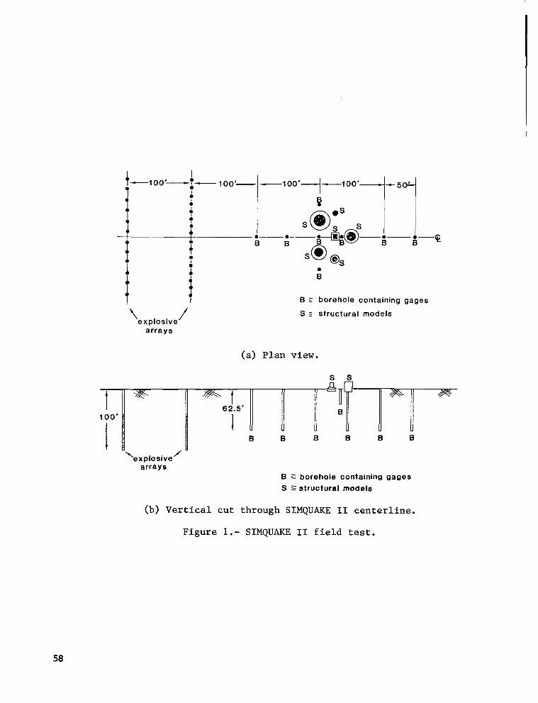
- I 100'

1

t r i

0

B

? t B borehole containing gages

\ 1 S 5 structural models explosive

arrays

(a) Plan view.

7

'explosive arrays

llI" s s

I B B B B B B

B Z borehole containing gages S S structural models

(b) Vertical cut through SIMQUAKE I1 centerline.

Figure 1.- SIMQUAKE I1 field test.

58

Figure 2.- Typical scaled structure.

Figure 3.- Two-dimensional multi-grid example.

59

STRUCTURE air-structure interface

I

I VOID I VOID

1" - ":

I

I I

I """"""""""""""""""

f soil-structure interface

s OIL

(a) Schematic using no slidelines and one grid.

STRUCTURE

) tied slideline. L""

soil-structure interface

SOIL

/ €Irid+'

(b) Schematic using one slideline and two grids.

Figure 4.- Schematics of SIMQUAKE mesh.

60

free slide line tied slideline +3

tied slide lines

(a) At bottom of flexible structure only.

7 free slideline \ [RiaJ . ..

. . . . , , . . ..

(b) All around flexible structure.

Figure 5.- Debonding/rebonding of a flexible structure.

rigid body wall interaction line

Figure 6 . - Debonding/rebonding all around rigid structure.

61

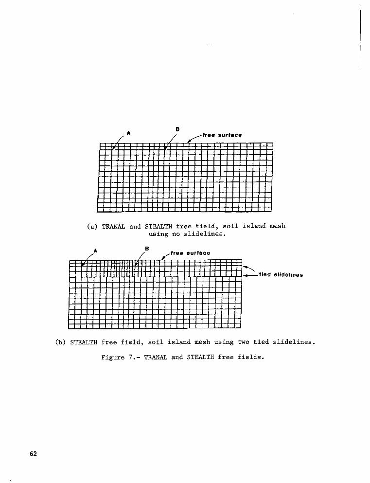
(a) TEUNAL and STEALTH free field, soil island mesh using no slidelines.

B

\ - t ied slidelines

(b) STEALTH free field, soil island mesh using two tied slidelines.

Figure 7.- TRANAL and STEALTH free fields.

62

TRANAL STEALTH

40.0 4

m W s e 4 v

4 0

3 al P

x

4 rn Y C

-* U 0 zz

0.0

-10.0

-20 .o ~

-30.0

n

I I

0.0 1.0 2 . 0 3.0

Ill1 I I I I I I I I IIII I I I I

I I I -45 .O time (sec) 0 . 0 1 .o 2 . 0 3 .O

time (sec)

(a) Horizontal velocity histories for 3.0 seconds from TRANAL and STEALTH output at location A (see Fig. 7).

1 5 . 0 i 10.0 ~

5-01 0 .o

-10.0 -5-03 -15.0 4

STEALTH

coarse mesh

0 .o 0.5 1 .o

STEALTH fine mesh

0 W VI

U

a

W

-5 4 v

15.0

10.0

5.0

0.0

-5.0

-10.0

-15.0

0.0 0.5 1 .o time (sec) time (sec)

(b) Vertical velocity histories for 1.0 second from two STEALTH meshes at location B (see Fig. 7).

Figure 8.- Comparison of velocity histories for elastic free field simulations.

63

MANGE - 150' RANGE - 300'

(a) TRANAL mesh.

CONCRETE

0 BACKFILL

RAWGE I 150' RANGE - 300 '

(b) STEALTH mesh.

Figure 9.- Comparison of TRANAL and STEALTH meshes with gapping elements, or zones, next to flexible structure.

64

1

-40 .00 t

60.00

40. 00 h -0

h C 4 0 O 20.00

+ %

:%

0a l o m d

Ll 0 .88

l-l o m * Q) -30.08 L l G al 4 3 - -40.00

-69.00 e . ee e . 5 8 1.00 1.50 2. e0 2 . 5 0 3.80

Time (sec)

Figure 10.- Comparison of three velocity histories on the flexible structures.

65

I

COMBUSTION - STRUCTURAL INTERACTION I N

A VISCOELASTIC MATERIAL*

T. Y. Chang and J. P. Chang Department of Civil Engineering

The University of Akron, Akron, Ohio

M. Kumar and K. K. Kuo Department of Mechanical Engineering

The Pennsylvania State University University Park, Pennsylvania

SUMMARY

The e f f ec t o f i n t e rac t ion between combustion processes and structural deformation of so l id p rope l lan t w a s considered. The combustion analysis w a s performed on the basis of deformed crack geometry, which was determined from the s t ruc tu ra l ana lys i s . On t h e o t h e r hand , input da ta for the s t ruc tura l ana lys i s , such as p ressure d i s t r ibu t ion a long the c rack boundary and ab la t ion v e l o c i t y of the c rack , were determined from the combustion analysis. The i n t e r - ac t ion ana lys i s w a s conducted by combining two computer codes, a combustion analysis code and a general purpose f ini te e lement s t ructural analysis code.

INTRODUCTION

In recent years , much at tent ion has been focused on the inves t iga t ion of the coupl ing e f fec t between combustion phenomenon and mechanical behavior of solid propel lant . The so lu t ion of problems of th i s type can fur ther be t te r unders tand- ing of t h e t r a n s i e n t combustion processes inside solid propellant cracks, which may s igni f icant ly a f fec t the per formance of a rocket motor. The combustion phenomenon ins ide the c rack of so l id p rope l lan t is strongly influenced by the crack geometry a s t h e material i s being deformed and burned away. Generally, there are two major reasons for a l terat ion of the crack geometry: 1) mass l o s s due t o g a s i f i c a t i o n of propel lant surface a long the crack during the combust ion process , and 2 ) mechanical deformation of the propellant due to p ressure .

On one hand, both the burning rate and mechanical deformation a r e governed by pressure ac t ing on the c rack sur face . On the o the r hand, a change i n c r a c k s i z e w i l l cause the p ressure d i s t r ibu t ion to vary . The p res su re d i s t r ibu t ion will strongly influence the deformation and stress concentration a t the c rack

*Research sponsored by t h e Power Program of the Off ice of Naval Research Arlington, Va . , under Contract No. N00014-79-C-0762. The support of D r . R. S. Miller is grate- f u l l y acknowledged. A p a r t o f t h i s work w a s performed under a previous contract sponsored by D r . R. L. Derr of NWC. H i s support is also appreciated.

67

t i p , which i n t u r n w i l l a f f e c t t h e manner of the crack propagation. It is , therefore , apparent tha t the p ressure d i s t r ibu t ion and the change in c rack geometry are strongly interdependent.

In the past , combust ion and s t ruc tura l ana lyses o f so l id p rope l lan t were conducted independently, with the result t h a t i n t e r a c t i o n e f f e c t s were completely ignored. As noted above, such interact ion effects can be qui te important , especi- a l l y when the deformation is l a r g e as compared to the or iginal crack-gap width. The deformation response of the material is categorized as l i n e a r l y v i s c o e l a s t i c . It is, the re fo re , t he i n t en t of t h i s pape r t o p re sen t a method o f ana lys i s fo r t he combust ion-s t ruc tura l in te rac t ion in a l i n e a r v i s c o e l a s t i c medium. To t h i s e n d , three major tasks are involved: 1) combustion analysis to model t h e t r a n s i e n t combust ion process , 2) viscoelast ic analysis in conjunct ion with moving boundary, and 3) l inkage of t h e two analyses.

For t h e combust ion analysis , invest igat ions of cer ta in aspects of combustion processes have been made. Taylor [ l] conducted experimental tests to s tudy t he convective burning of porous propellants with closed- and open-end boundary conditions. Belyaev e t a l . [2] showed that the burning of propel lant inside a narrow pore may lead to an excess pressure bui ldup. In a la ter s tudy, Belyaev e t a l . [3] made a series of experimental tests to determine the dependence of flame-spreading rate on crack geometry, propellant properties, boundary conditions, and combustion chamber pressures. Cherepanov [ 4 ] s t a t e d t h a t a s a r e s u l t of t h e impeded gas flow i n a suff ic ient ly narrow and long cavi ty , the pressure reaches such high values that the system becomes unstable. From h i s work, Godai [SI ind ica ted tha t there i s a threshold diameter or cr i t ical width of a uniform cavity below which flame w i l l not propagate into the crack. Krasnov et a l . [6] inves t iga ted the ra te o f pene- t r a t i o n of combustion i n t o t h e p o r e s of an explosive charge. Jacobs e t a l . [7,8] s tudied the p ressure d i s t r ibu t ion in burn ing c racks tha t s imula te the debonding of sol id propel lant f rom the motor casing.

Although results of previous experiments were of i n t e r e s t , no sound theore- t i c a l model was developed. In this s tudy, a t h e o r e t i c a l model was establ ished f o r p r e d i c t i n g r a t e of f lame propagat ion, pressure dis t r ibut ion, and pressuriza- t i on rate ins ide the c rack . Two sets of coupled p a r t i a l d i f f e r e n t i a l e q u a t i o n s were obtained: one from mass, momentum, and energy conservation of the gas phase of the propel lant product in the void region adjacent to the crack surface; the o the r from consideration of solid-phase heat conduction. Due to the mathematical complexity of governing equations and boundary conditions involved, the finite d i f fe rence method w a s used to obtain the solut ion for the combust ion analysis . In the numerical solut ion, the boundary condi t ions, which vary with time, are s p e c i f i e d i n terms of the changing crack geometry, which i n t u r n i s found from the s t ruc tura l ana lys i s . In addi t ion , the p ressure d i s t r ibu t ion a long the c rack sur - face, varying as a funct ion of time, was obtained from the analysis and w a s used as i n p u t f o r t h e s t r u c t u r a l a n a l y s i s .

For s t ruc tura l ana lys i s , d i f fe ren t approaches have been taken prev ious ly in so lv ing ( ana ly t i ca l ly o r numer i ca l ly ) s eve ra l moving boundary problems i n l i n e a r v i s c o e l a s t i c i t y . Lee e t a l . C9l obtained a s o l u t i o n f o r t h e p r e s s u r i z a t i o n of an annihi la t ing viscoelast ic cyl inder contained by a n e l a s t i c c a s i n g i n which the mater ia l w a s assumed t o be a Kelvin model i n s h e a r and incompressible in bulk. Arenz e t a l . [ l o ] performed a s i m i l a r a n a l y s i s f o r a sphere. Corneliussen e t

68

al . [11,12] presented so lu t ions for a sp inning , annih i la t ing , v i scoe las t ic cyl inder with f ree outer boundary. Since the cons t ra in ing case w a s not included i n t h e i r a n a l y s e s , t h e stress d i s t r i b u t i o n was independent of the material pro- p e r t i e s . With the assumption of a standard linear s o l i d model, Shinozuka [13] presented the ana ly t ica l so lu t ion for a case-bonded p res su r i zed v i scoe la s t i c cyl inder . More general ized solut ions were obtained by Rogers e t a l . [14] f o r a class o f l i n e a r v i s c o e l a s t i c problems by using the numerical in tegrat ion scheme. Schapery [15] also developed a general method for so lv ing moving boundary problems. In h i s approach , the moving boundary condition w a s replaced by a f i c t i t i o u s non- moving boundary subjected to a time-dependent pressure. Later, Christensen e t al . [16] obtained a series s o l u t i o n f o r t h e stresses of t h e same problem. As noted above, most of t h e a n a l y t i c a l s o l u t i o n s were ava i l ab le fo r v i scoe la s t i c problems of simple geometry. For complex geometry, t he f i n i t e e l emen t method has proven t o b e most useful.

Applicat ion of the f ini te element method fo r so lv ing v i scoe la s t i c problems i s not new; r epor t s of such work can be found, for instance, in references [17-201. However, most of the previous work did not consider the effect of moving boundary, an impor tan t fea ture for the s t ruc tura l ana lys i s o f so l id p rope l lan t . Sankaran and Jana [21] presented a technique for the solving of axisymmetric viscoelastic so l id s w i th moving boundary. In their approach, the f ini te e lement mesh corresponding to t he new boundary w a s re -genera ted , whi le the s t ress -s t ra in h i s tor ies and mater ia l p roper t ies were assumed t o be carried over from those of the previous time increment. This assumption is val id only i f the t ime increment i s very small. An algorithm for automatically tracking ablating boundaries was given by Weeks and Cost [22]. A l l previous work deal ing with moving boundary viscoelast ic problems lacks both the appropriate treatment of material p rope r t i e s , and s t r e s s - s t r a i n h i s t o r i e s f o r t h e newly generated mesh. It is the purpose of this paper to present such a treatment.

Three major features must be i nc luded i n t he s t ruc tu ra l ana lys i s fo r a s o l i d propellant: 1) proper modeling of v i scoe las t ic behavior , 2) tracking of ab la t ing boundary in o rde r t o gene ra t e new f i n i t e element meshes, and 3 ) t r e a t - ment of the material r e sponses ( i . e . , s t r e s s - s t r a in h i s to r i e s and material properties) f o r t h e new mesh. All of these features have been incorporated into a nonl inear f ini te e lement program ca l l ed NFAP [231 . Combustion and s t r u c t u r a l programs were combined i n o r d e r t o make poss ib le an in te rac t ion ana lys i s . Numeri- cal resul ts are presented to demonstrate the effect of i n t e r a c t i o n between combustion and structural responses of the material.

COMBUSTION ANALYSIS

The t h e o r e t i c a l model w a s developed to simulate the combustion phenomenon i n s i d e a propel lant crack, which i s l o c a t e d i n a t ransverse d i rec t ion to the main flow of the rock chamber. During the course of der ivat ion, the fol lowing assumptions are made:

1) All chemical reactions occur near the propellant crack surface, and t h e combustion zone i s so t h i n t h a t i t is considered a plane.

2) Rate processes a t the p rope l l an t su r f ace a r e quas i - s t eady i n t he s ense t ha t c h a r a c t e r i s t i c times associated with the gaseous f lame and preheated pro- p e l l a n t are shor t i n comparison t o t h a t of pressure t rans ien t var ia t ion .

69

3) Gases flowing i n t h e p r o p e l l a n t c r a c k obey the Claus ius o r Noble-Abel equation of state.

4 ) Bulk flow i n t h e p o r e is one-dimensional C241.

To describe gas-phase behavior inside a sol id propel lant crack, mass, momentum, and energy equations i n unsteady, quasi-one-dimensional forms have been developed, based upon the ba l ance o f f l uxes i n a con t ro l volume within the propellant crack.

The mass conservation equation is

The momentum conservation equation is

The energy conservat ion equat ion wri t ten in terms of the to ta l s tored energy ( i n t e r n a l and k i n e t i c ) p e r u n i t mass, E ; i s

The conservation equations are fur ther s impl i f ied by an order of magnitude a n a l y s i s i n which the fol lowing terms a re neg l ig ib l e : 1) forces between molecules due to viscous normal stress i n a x i a l d i r e c t i o n ; 2) v iscous diss ipat ion and rate of work done by the force caused by viscous normal stresses in t he ene rgy equation; and 3) axial heat conduct ion between gas molecules in the energy equation.

The propellant surface temperature a t a f ixed locat ion a long the crack before the a t ta inment o f ign i t ion is calculated from the solid-phase heat conduction equation written in unsteady one-dimensional form:

70

where the l eng th va r i ab le y is measured perpendicular to the loca l p rope l lan t crack surface. Ini t ia l and boundary condi t ions are

T (0, Y) = T

T ( t , m) = T

P r P i

P r P i

(5)

(6)

The heat conduction equation is solved by using an integral method [25] which employs a third-order polynomial, or by direct numerical solution of Eqs. (4-7) with var iable mesh s i ze i n t he subsu r face .

For the gas phase, the Noble-Abel equation is used for the equation of state:

The gas-phase equations, i. e. Eqs . (1) , ( 2 ) and ( 3 ) , are non-linear, inhomo- geneous, p a r t i a l d i f f e r e n t i a l e q u a t i o n s . Along w i t h t h e p a r t i a l d i f f e r e n t i a l equat ion for the so l id phase (Eq. ( 4 ) ) , they are solved simultaneously, using the f i n i t e d i f f e r e n c e method. The der ivat ion descr ibed above w a s implemented i n t o a computer program, crack combustion code (CCC) by Kuo e t a l . [ 2 6 ] .

STRUCTURAL ANALYSIS

To conduct the s t ruc tura l ana lys i s o f the so l id p rope l lan t , th ree main f ea tu res must be included in the numerical formulations: 1) modeling of v i s c o e l a s t i c material behavior, 2) simulation of ablating boundary, and 3) treatment of material responses by an interpolation scheme. Each f e a t u r e is out l ined below.

Viscoe las t ic Material Model

The material behavior of the sol id propel lant is assumed to be viscoelastic i n shear and e las t ic i n bulk. Only the isothermal condi t ion is considered. The s t r e s s - s t r a in r e l a t ions w i th ze ro i n i t i a l cond i t ions . are w r i t t e n i n two pa r t s .

1) Shear behavior:

t sij = I Gl(t-t') - d t ' e i j ( t ' ) d t ' (9)

0

71

where GI is the relaxation modulus in shear. For most viscoelastic materiaxs, it is usually considered

M

m= 1 = go + C gm e -Bmt

2,) Bulk behavior:

D = 3K kk

As discussed in [27], the incremental stress-strain relations in matrix form are written as

where T {Au) = AD^^. AD^^^ A‘rZ3’ AD,,)

= Asl1} M

= Bm ‘mc22’ m 33’ m 23’ m 11 Ct Ct Ct } m=l

and

IDVE] =

Furthermore

symmetric

M

(K+ 7 A ) 0 (K- - 2 1 3 *)

A 0 2 -

B m = l - e -BmAt

(K+ f A)

and the term mCij has a recursive relationship, i.e., t

72

-$,At)

ct = e -BmAt C t - A t + gm(l-e m i j m i j $,At e' i j

t t - A t i j i j i j

e' = e - e

The advantage of Eq. (19) is t h a t a l l of the s t ra in history can be obtained by re fer r ing on ly to in format ion i n the previous t i m e s tep, thus reducing computer s torage and numerical calculations.

From t h e v i r t u a l work p r inc ip l e and t he r e l a t ionsh ip o f Eq. ( 1 2 ) , t h e f i n i t e element equilibrium equations for a t y p i c a l t i m e i n t e r v a l [ t , t + A t ] can be derived as

where m

and {fo} = [BIT {u0} dv

Simulation of Ablating Boundary and Mesh Generation

Burning of the propellant causes a s ignif icant change in geometry, thus present ing compl ica t ions in f in i te e lement s t ruc tura l ana lys i s . The e f f ec t o f ab la t ing boundary is accounted for by redef in ing the f in i te e lement mesh a t s p e c i - f i e d time intervals . This involves two s t ages of ca l cu la t ions : 1) tracking of the ablat ing boundary, and 2) generat ion of new f i n i t e element mesh. With some modifications, the procedures adopted herein are s imi la r to those p resented i n [22].

Consider a s t r u c t u r a l geometry with ablat ing boundary. The spa t i a l pos i - t i o n s of the ablating boundary are determined by the ab la t ion ve loc i t i e s which a r e found from t h e combustion analysis a t d i s c r e t e times. It is assumed t h a t the ab la t ion occurs a lways in the d i rec ton normal t o t h e boundary. For struc- t u r a l a n a l y s i s , t h e entire surface is div ided in to an ab la t ing par t and a non- ab la t ing pa r t ; e ach pa r t is formed by d iscre te l ine segments jo in ing a t the nodes of t h e f i n i t e element mesh. The new pos i t ion of each l i ne segment is located from the given ablating velocity. Consequently, the new boundary nodes are determined by ca lcu la t ing the in te rsec t ions o f two subsequent new l i n e segments. Likewise, the nodes a t the i n t e r sec t ions o f new ablating and non-ablating boundaries are then determined.

During the locat ing process , however, some of the boundary nodes may not l i e on t h e new boundary and thus must be eliminated. If the distance from t h e t i p of t h e normal vector a t a new nodal pos i t ion to any node on t h e o r i g i n a l boundary is less than t he va lue o f t he normal i t s e l f , t h e node is removed.

73

I n g e n e r a l , t h e t o t a l number of nodes on the boundary a t d i s c r e t e times w i l l be different because some of the nodes have been removed. However , i n t he ana lys i s i t is more convenient to generate a f i n i t e element mesh similar t o the o r ig ina l one so that in te rpola t ion of material response can be made. One way to accomplish this is by keeping the number of boundary nodes constant. Consequently, t h e boundary nodes are redis t r ibuted between two d iscont inui ty po in t s which are s p e c i f i e d i n t h e i n p u t d a t a i n such a way t h a t t h e l e n g t h s of t h e new l i n e segments have t h e same r a t i o as those o f t he o r ig ina l l i nes .

Once t h e new boundary nodes are defined, an automatic mesh generation scheme i s used t o create the i n t e r io r nodes fo r fu r the r ana lys i s . Because of i t s f l e x i b i l i t y i n o b t a i n i n g a desirabEe mesh, a Laplacian-isoparametric grid generation scheme [ 281 is u t i l i z e d . However, t h i s method is l i m i t e d t o a geometry bounded by fou r s ides . A f i n i t e element mesh is shown in F ig . 1. The coordinates of t h e i - t h i n t e r i o r node can be expressed in terms of those of neighboring nodes by

where w is the weight ing fac tor for ad jus t ing the d i s t r ibu t ion of in te r ior nodes , and 0 5 ~ 5 1 .

Se t t i ng up the equat ions for each in te r ior node y i e l d s two systems of simul- taneous equations. It is observed that the resul t ing systems of equat ions are banded and symmetric. The Gaussian elimination scheme is employed t o s o l v e f o r the coordinates of the inter ior nodes.

In te rpola t ion of Material Responses

As seen from Eq. (16) , the stress increment AU f o r t h e time i n t e r v a l [ t , t+At] varies with material p r o p e r t i e s a n d w i t h t h e s t r a i n h i s t o r y a t b o t h current and previous time steps. When the region of an element changes over a period of time due to ab l a t ion , t he ma te r i a l r e sponse h i s to ry of t h e new elements is l o s t and must be determined by an in te rpola t ion procedure from t h e o l d elements a t previous time steps. Accordingly, the interpolation procedure is ca r r i ed out on th; element level. For calculat ions, the material responses are separated i n t o two groups: the f i rs t includes such var iables evaluated a t the Gaussian in tegra t ion po in ts , i . e . , ADi. , A E ~ . and Ci. ; the second includes the nodal displacements which are e v a l d t e d a$ noday pa in ts . In the p resent ca lcu la t ions , two l i m i t a t i o n s are imposed: 1) eight-node quadrilateral elements are used throughout the analysis ; and 2) the four sides of each element remain straight before and a f t e r a b l a t i o n .

1) Interpolat ion of Gaussian var iables - It i s noted tha t the quadra t ic d i s - placement approximation of an eight-node element yields a l i n e a r s t r a i n v a r i a - t i on . With t h i s fact i n mind, the quant i t ies o f Gauss ian var iab les a t nodal po in ts a re f i r s t eva lua ted for every o ld e lement . As shown i n Fig. 2a , b , th is can be done by using the l inear isoparametr ic shape funct ions, namely,

74

4 - wk' = z hi(rL, Si) * w; k = 1, 2,

i=l

where h, = 1/4(1 + r , r ) ( l + s,s) i = 1, 2, 3 , 4 I

For each new point are known. computed by using

I I

e lement , the loca l coord iza tes ( r , s) of The global coordinates, (yk, zk) ,kef t h a t the following equations:

3, 4

the k-th Gaussian poin t a re , therefore ,

4

L - 'k

= p hi ( rk , sk) * zi i= 1

After (yk, ) are found, the old e lement to which the point belongs must be i d e n t i f i e d . kA search process based upon the va lues o f r ' and s ' is developed for this purpose. The search starts from the old element which corresponds t o t h e neighboring elements. Equations for such calculations are given by

L

Fig. 2c shows how to i den t i fy t he e l emen t t o which the po in t s , (r', s f ) , belong. Once the loca t ion of the po in t is ver i f ied , an in te rpola t ion procedure i s performed, using the relationship

4

2) I n t e r p o l a t i o n of nodal displacements - A similar procedure to that explained above is also used to determine the posi t ion of t h e node in ques t ion wi th re fe r - ence to the old element. However, the in te rpola t ion procedure in Eq. (26) is no longer necessary since the nodal displacements are known. The nodal displacements of the new mesh are computed from

8

i=l di = 1 h i ( r ' , s ' ) * di'

where h. are the s tandard quadrat ic isoparametr ic shape funct ions. 1

75

All formulat ions discussed in this sect ion have been implemented i n t o a general purpose nonlinear f inite element program c a l l e d NFAP for conducting v iscoe las t ic ana lys i s o f so l id p rope l lan t wi th ab la t ing boundary . Some numer- i c a l examples are presented in a la ter sect ion.

COUPLING EFFECT

For s t ruc tu ra l ana lys i s , t he boundary condi t ion a long the c rack geometry i s defined by pressuredis t r ibu t ionwhich varies with t i m e , and ablat ion veloci ty; both are determined from combustion analysis. In the combustion analysis, the regress ion ra te o f the p rope l lan t i s dependent on the deformed crack geometry. Therefore, the two processes are s t rongly interdependent . Such a coupl ing e f fec t is obtained by combining the ana lys i s o f two computer programs: a crack combus- t ion code (CCC) and a s t ruc tura l ana lys i s code (NFAP). Both codes were developed independent ly to fac i l i t a te program v e r i f i c a t i o n s . Linkage of t h e two codes w a s made subsequently.

The coupl ing effect considered in the present analysis i s l i m i t e d t o t h e major parameters, namely pressure loading, ablat ion veloci ty , and crack deforma- t ion . Pressure and ab la t ion ve loc i ty a re ca lcu la ted by t h e CCC a t each nodal point located on a one-dimensional grid along the length of the crack. The ana lys i s of crack combustion incorporates the crack geometry variation caused by both mechanical deformation and mass l o s s through gasif icat ion of the propel lant surface. Once the gas-phase equat ions are solved and the pressures and ablat ion ve loc i t i e s a long t he c r ack are ca lcu la ted for a given t i m e t , the da ta are trans- f e r r e d t o t h e NFAP as the input information. NFAP then simulates the updated crack geometry from t h e a b l a t i o n v e l o c i t i e s and generates a new f i n i t e element mesh. With the new mesh and pressure data , NFAP updates the s t i f fness mat r ix and i n t e r - po la tes material responses for conducting a q u a s i - s t a t i c a n a l y s i s a t time t . After obtaining the deformation, the change i n t h e c r a c k w i d t h a t e a c h f i n i t e d i f f e r e n t node is calculated and added to the exis t ing crack width. Since the crack width is the input o f the combustion ana lys i s , one cycle of calculat ions is thus completed. The same procedure i s followed for every specified time increment.

For program v e r i f i c a t i o n and demonstration of i ts ana lys i s capab i l i t y , t h ree sample problems were run e i ther by NFAP alone ur i n t h e combined NFA.P/CCC program. The r e s u l t s of t he ana lys i s a r e d i scussed i n t he fo l lowing . The numerical resul ts obtained from CCC alone are contained in reference [ 26 ] .

1. A Reinforced Thick-walled Cylinder

Figure 3 shows a cyl inder of viscoelast ic mater ia l bonded by a s teel casing and subjec ted to a s tep-funct ion internal pressure. The example w a s s e l ec t ed because i t i s composed of two d i f f e r e n t m a t e r i a l s and t h e a n a l y t i c a l r e s u l t s a r e r ead i ly ava i l ab le fo r comparison. Only five eight-node axisymmetric elements were used to model the cyl inder . The mater ia l p roper t ies of t h e e las t ic casing a r e

E = 2.068 x 10 MPa 6 v = 0.3015

76

I I 1111I I I I1 II I

I The material p rope r t i e s o f t he v i scoe la s t i c co re are defined by

I

K = 689.5 MPa G1 = 51.71 * exp (-0. l t ) MPa

In F ig . 4 , t he va r i a t ions of c i rcumferent ia l stresses with t ime are p l o t t e d f o r compar ison wi th the ana ly t ica l so lu t ion ob ta ined in [ g ] . It is observed that both solutions agree very closely. This problem w a s analyzed previously by Zienkiewicz e t a l . [ 1 8 ] , u s i n g s t r a i n rate formulat ion of the f ini te e lement method. However, the formula t ion presented in the p resent paper i s more e a s i l y incorpora ted in to the NFAP program.

2. A Star-shaped Solid Rocket Motor

AS an appl ica t ion of the p resent approach in dea l ing wi th the moving boundary, a star-shaped solid rocket motor w a s analyzed by assuming both a constant and ablating inner boundary. The configurat ion and f ini te e lement mesh are shown i n Fig. 5, and t h e material propert ies of outer casing and inner propel lant are i d e n t i c a l t o t h o s e of t h e f i r s t example. Taking advantage of t h e symmetry condition, only a 3O0-sector w a s modeled by f i n i t e element mesh. The contours of maximum compressive stress analyzed by constant inner boundary a t v a r i o u s times are shown i n Fig. 5. Comparing the p re sen t r e su l t s w i th t hose o f [ 181, i t is ev iden t t ha t t he gene ra l pa t t e rn i s q u i t e similar b u t t h a t some small d i f fe rences do ex is t . S ince the geometry of the rocke t motor in [18] w a s no t c lear ly def ined , the difference in dimension used in these two analyses could be the cause of such deviat ions.

The ac tua l case of a so l id rocke t motor can be modeled more closely by con- s ide r ing t he i nne r boundary being ablated. Figure 6 shows the contours of maximum compressive stress predicted by NFAP, using the option of moving boundary. The resu l t s ob ta ined are q u i t e d i f f e r e n t from those of [la]. However, observing the differences between Figs. 5 and 6, w e can conclude that the resul ts obtained by NFAP are qui te reasonable . The so lu t ion reveals tha t t he h igh stress region obtained for ablat ing boundary propagates fas ter than that wi th non-ablat ing boundary.

3. A Propellant Crack Specimen

A s a f i n a l example, a propellant crack sample w a s analyzed, using the combined NTAP/CCC program to demonstrate the coupl ing effect . The i n i t i a l geometry and f i n i t e element mesh generated by NFAP is given i n F i g . 7 . The crack is 0.15 m l ong and t he i n i t i a l gap-width i s 0.89 mm. The web thickness i s 8 nun a long the crack and 20 mm a t t h e t i p . Because of symmetry, only half of the Sample w a s modeled by 80 p lane s t ra in e lements . The shear re laxa t ion modulus of the p rope l lan t w a s assumed t o b e

Gl(t) = 1.461 + 7.43 * exp (-.095t) MPa; and K = 4,826 MPa.

Calcu la ted p ressure d i s t r ibu t ions a t var ious times, from t h e CCC alone, are given i n Fig. 7. The burning phenomenon of the propel lant can be br ief ly descr ibed as follows. The p r e s s u r e i n t h e chamber increases wi th t i m e , causing the hot gases to pene t ra te fur ther in to the c rack . As time passes , the p ressure wave travels along the crack and is reflected from the closed end. A t about

77

200 us, t he p re s su re f ron t has a l r eady r eached t he t i p and is ref lec ted , caus ing pressure a t t h e t i p t o increase.

Figure 8 shows the resu l t s ob ta ined f rom the combined NFAP/CCC program. During t h e i n i t i a l p e r i o d , t h e g e n e r a l t r e n d o f t h e p r e s s u r e d i s t r i b u t i o n is simi- la r t o t h a t from convective burning analysis alone. However, as time progresses , no t iceable d i f fe rences between the two cases begin to appear. Up t o 200 us , the pressures obtained f rom the combined ana lys i s are lower, except near the crack entrance region. A t t = 300 us, two pressure peaks appear. A t t = 325 us, th ree pressure peaks appear. These pressure peaks are caused by t h e p a r t i a l c l o s u r e of t h e gap. The deformation pattern of the propellant is qui te i r regular because o f t he uneven d i s t r ibu t ion o f t he p re s su re a long t he c r ack su r f ace . The elements a t the c rack en t rance are compressed by the h igh chamber pressure, which results i n t h e p r o p e l l a n t b e i n g pushed into the crack. Since chamber pressure increases more quickly than pressure inside the crack, the propel lant is pushed toward the lower pressure region inside the crack. The mechanical deformation of the propellant causes narrowing of the crack width, and consequently results in a l o c a l c r ack c losu re . Th i s loca lgap c losu re man i fe s t s i t s e l f i n a pressure peak. The loca l ized pressure peaks o r gap closures move along the crack. A t t = 3 2 5 u s , t h i s loca l ized pressure phenomenon becomes evident a t x / L = 0.167, 0 . 4 3 3 , and 0 . 6 3 3 .

CONCLUSION

The computer program fo r eva lua t ing t he coup l ing e f f ec t between convective burning and structural deformation w a s developed by combining t h e Crack Combustion Code and a Nonlinear Finite-Element Analysis Program. In s t r u c t u r a l a n a l y s i s , t he l i nea r v i scoe la s t i c material model, toge ther wi th the capabi l i t i es o f simu- l a t i n g a b l a t i n g boundary and in t e rpo la t ing material responses , was considered. Also, the coupl ing e f fec t es t imated by the combined ana lys i s shows some s i g n i f i - can t in te rac t ion between the combustion and mechanical deformation. This phenomenon w i l l be ver i f ied fur ther by future experiments.

78

SYMBOLS

1. Combust ion Analysis

A = cross-sectional area of crack

B = body force

b = co-volume

c = specific heat at constant pressure

E = total stored energy

h = local convective heat-transfer coefficient

h = local convective heat-transfer coefficient over propellant surface

hew= local convective heat-transfer coefficient over nonpropellant port wall hf = enthalpy of combustion gas at adiabatic flame temperature

ph = burning perimeter

Pw = wetted perimeter of port

p = static pressure

R = specific gas constant for combustion gases

1: = burning rate of solid propellant, including erosive burning contribution

T = temperature (without subscript, static gas temperature)

Tf = adiabatic flame temperature of solid propellant

T = initial propellant temperature

T = propellant surface temperature

P

X

P

- C - CP -

b

Pi

PS

Tws = nonpropellant wall surface temperature

t = time

u = gas velocity

Vgf= velocity of propellant gas at burning surface

x = axial distance from propellant crack opening

y = perpendicular distance from propellant surface into solid

a = thermal diffusivity

79

y = ratio of specific heats

X = thermal conductivity

IJ = gas viscosity

P = density (without subscript, gas density)

T = shear stress on port wall

T = normal viscous stress

0 = angle measure, in a counterclockwise direction, at lower side of

W

xx

W propellant, degree

Subscripts

i = initial value

pr = solid propellant (condensed phase)

c = rocket chamber

2 . Structural Analysis

'ij = stress deviators

e ij = strain deviators

' ij = stress tensor

G1 = shear relaxation modulus

K = bulk modulus L

( )L = a quantity at time t

{Aa) = incremental stress

IAE) = incremental strain

{ao} = equivalent initial stress vector due to viscoelastic behavior

[KJ = stiffness matrix

c lT = transpose of matrix

M = number of terms of series in relaxation modulus

80

go = ) gm = I material constants in relaxation modulus {Av} = increment of nodal displacement vector

[Dv,l = viscoelastic material matrix

[B] = strain-nodal displacement transformation matrix

w' = values of Gaussian variables at k-th integration point referred -

to old element

W' i = values of Gaussian variables at i-th nodal point referred to old element

(rk',sk') = local coordinates of k-th integration point referred to old element

(yi,z ) = global coordinates of i-th nodal point referred to new element i Di = i-th nodal displacement referred to new element

Dit = i-th nodal displacement referred to old element

(r',s') = local coordinates of point in equation referred to old element

81

I-

1.

2.

3.

4.

5.

6.

7.

8.

9.

10.

11.

12.

13.

REFERENCES

Taylor, J.W.: The Burning of Secondary Explosive Powders by a Convective Mechanism. Trans. Farad. SOC. 58, 1962, p. 561.

Belyaev, A.F.; Korotkov, A . I . ; Sulimov, A.A.; Sukoyan, M.K.; and Obemin, A.V.: Development of Combustion i n an I so la t ion Pore . Combustion, Explosion and Shock Waves, Vol. 5, Jan.-March 1969, pp. 4-9.

Belyaev, A.F.; Bobolev, V.K.; Korotkov, A.A.; Sulimov, A.A.; and Chuiko, S.V.: Development of Burning i n a Single Pore, Transi t ion of Combustion of Condensed Systems to Detonation, Chap. 5, Pt.A.,. Science Publisher, 1973, pp. 115-134.

Cherepanov, G.P.: Combustion i n Narrow Cavities. J. of Appl. Mech., Vol. 11, 1970, pp. 276-281.

Godai, T.: Flame Propagation into the Crack of a Solid-Propellant G r a i n . AIAA Journal, Vol. 8, July 1970, pp. 1322-1327.

Krasnov, Yu. K.: Margulis, V.M.; Margolin, A.D.; and Pokhil, P.F.: Rate of Penetration of Combustion into the Pores of an Explosive Charge. Combus- tion, Explosion, and Shock Waves, Vol. 6, July-Sept. 1970, pp. 262-265.

Jacobs, H.R.; Williams, M.L.; and Tuft, D.B.: An Experimental Study of the Pressure Distr ibut ion in Burning Flaws in Sol id Propel lan t Gra ins . Univ. of Utah, S a l t Lake City, Utah, Final Report to A i r Force Rocket Propulsion Laboratory, AFRPL-TR-72-108, UTEC DO 72-130, Oct. 1972.

Jacobs. H.R.; Hufferd, W.L.; and Williams, M.L.: Further Studies o f t he Critical Nature of Cracks in Solid Propellant Grains, AFRPL-TR-75-14, March 1975.

Lee, E.H. ; Radok, J .R.M. ; and Woodward, W.B.: Stress Analysis for Linear Viscoelastic Material . Trans. SOC. Rheol., Vol. 3, 1959, pp. 41-59.

Arenz, R . J . ; and Williams, M.L.: The Stresses in an E las t ica l ly Reinforced Pressurized Viscoelastic Sphere with an Eroding Boundary. Proceedings 20th Meeting Joint Army-Navy-Air Force Physical Properties Panel, Johns Hopkins Univ., Baltimore, Md., 1961, p. 143.

Corneliussen, A.H.; and Lee, E.H.: Stress Distr ibut ion Analysis for Linear Viscoelast ic .Mater ia ls . Internat ional Union of Theoretical and Applied Mechanics Symposium on Creep, 1960, pp. 1-20.

Corneliussen, A.H.; Kamowitz, E.F.; Lee, E.H.; and Radok, J .R.M. : Visco- elastic Stress Analysis of a Spinning Hollow Circular Cylinder with an Ablating Pressurized Cavity. Trans SOC. Rheol., Vol. 7 , 1963, pp. 357-390.

Shinozuka, M.: Stresses i n a Linear Incompressible Viscoelastic Cylinder with Moving Inner Boundary. J. Appl. Mech., Vol. 13, 1963, pp. 335-341.

14. Rogers, T.G.; and Lee, E.H.: The Cylinder Problem i n V i s c o e l a s t i c Stress Analysis. Quart. Appl. Math., Vol. 22, 1964, pp. 117-131.

82

15.

16.

17.

18.

19.

20.

21.

22.

23.

24.

25.

26.

27.

28.

Schapery, R.A.: An Approximate Method of Stress Analysis for a Large Class of Problems in Viscoe las t ic i ty . Purdue Univ. Rept. A. and ES62-18, 1963.

Christensen, R.M.; and Schreiner, R.N.: Response to P re s su r i za t ion of a Viscoelastic Cylinder with an Eroding Internal Boundary, AIAA Journal, Val. 3, 1965, pp. 1451-1455.

Chang,: T.Y.: Approximate Solu t ions in L inear Viscoe las t ic i ty . Ph.D. Disser ta t ion, Dept. of Civi l Eng., Univ. of California, Berkeley, 1966.

Zienkiewicz, O.C.; Watson, M.; and King, I.P.: A Numerical Method of Viscoelast ic Stress Analysis . Int . J. Mech. Sc i . , Vol. 10, 1968, pp. 807-827.

White, J .L . : F i n i t e Element in Linear Viscoelast ic i ty . Proceedings of 2nd Conference on Matrix Method i n S t r u c t u r a l Mechanics, Ai r force F l igh t Dynamics Lab, Wright Pa t te rson AFB, Ohio, AFFDL-TR-68-150, 1968, pp. 489-516.

Gupta, K.K.; and Heer, E.: Viscoe las t ic S t ruc tures . S t ruc tura l Mechanics Computer Programs, Univ. Press o f V i rg in i a , Cha r lo t t e sv i l l e , 1974, pp. 207-225 - Sankaran, G.V.; and Jana, M.K.: Thermviscoelastic Analysis of Axisyrmnetric

Sol idPropel lant Grains . J. Spacecraft , Vol. 13, 1976, pp. 641-642.

Weeks, G.E. ; and Cost, T.L. : An Algorithm for Automatically Tracking Ablat- i ng Boundary. I n t . J. Num. Method. Engr., Vol. 14, 1979, pp. 441-449.

Chang, T.Y.; and Prachuktam, S.: NFAP - A Nonlinear Finite-Element Analysis Program. Dept. of Civil Engr. , Univ. o f Akron, Rept. No. SE76-3, 1976.

Kuo, K.K.; Chen, A.T.; and Davis, T.R.: Transient Flame Spreading and Combustion Process Inside a Solid Propellant Crack. AIAA Paper 77-14, AIAA 15th Aerospace Science Meeting, Jan. 1977.

Goodman, T.R.: Appl icat ion of Integral Methods to Transient Nonlinear Heat Transfer. Advances i n Heat Transfer, Vol. 1, Academic Press , New York, 1964, pp. 51-122.

Kuo, K.K.; Chen, A.T.; and Davis, T.R.: Convective Burning in Sol id-Propel lant Cracks. AIAA Journal, Vol. 1 6 , June 1978, pp. 600-607.

Chang, J . P . : F i n i t e Element Analysis of Linear Viscoelastic Solids. M.S. Thesis, Dept. of Civil Engr., Univ. of Akron, 1980.

Herrmann, L.R.: Laplacian-Isoparametric Grid Generation Scheme. J. of 'Engr. Mech. Div., Proc. of the ASCE, Vol. 102, Oct. 1976, pp. 749-756.

83

I

5

Figure 1.- Neighborhood of node i.

IrlS 1

I

3

(a 1 0 Gaussian ,points

o Node points

i /- "Old" element

"New" e 1 emen t

Figure 2.- I n t e rpo la t ion scheme.

84

Y

t Y

Top a n i S i d e View Po = 0.69 MPa

t- Figure 3.- Finite element mesh of a reinforced thick-walled cylinder.

85

- Closed form solution 0 NFAP solution

1 .

.8

.6

.4

.2

.o

- .2 0.5 0.6 0.7 0.8 - x/bo

0.9

t = 30

t = 10

t 5 s

Figure 4.- Reinforced cyl inder under internal pressure v a r i a t i o n of hoop stress.

86

Figure 5.- Finite element mesh and contours of maximum principal stress of a star-shaped rocket motor with fixed boundary.

87

Figure 6.- Contours of maximum principal compressive stress of a star-shaped rocket motor with moving boundary.

88

, Line of symmetry of the propellant crack

6oap - 0.89

300 - L - 0.15 m

200 1 t = 325 us

ff-" 300

0 0.2 0.4 0.6 1.(

Axial Distance, x/L

Figure 7.- Finite element mesh of a propellant crack and calculated pressure distributions for various times from the crack combustion code.

89

300

200

100

0 0 0.2 0.4 0.6 0.8 1.0

Axial Distance, x/L

Figure 8.- Calculated pressure distributions f o r various times from the combined crack combustion and non-linear finite-element analysis program.

90

ITERATIVE METHODS BASED UPON RESIDUAL AVERAGING

J. W. Neuberger

This paper concerns i terative methods for so lv ing boundary va lue p rob- l e m s f o r s y s t e m s o f n o n l i n e a r p a r t i a l d i f f e r e n t i a l e q u a t i o n s . The methods i n v o l v e s u b t r a c t i n g an average o f res idua ls f rom one approximat ion in o rder t o arrive a t a subsequent approximation.

The paper is d i v i d e d i n t o f i v e p a r t s . The f i r s t p a r t g i v e s two ab- s t ract methods i n H i l b e r t s p a c e . The second pa r t shows how t o a p p l y t h e s e methods to quas i l inear sys tems to g ive numer ica l schemes for such problems. The t h i r d s e c t i o n c o n t a i n s some s p e c i f i c a p p l i c a t i o n s . The f o u r t h p a r t con- t a i n s a d i scuss ion o f some p o t e n t i a l t h e o r e t i c matters r e l a t e d t o t h e i t e r a t i o n schemes. The f i n a l p a r t i n d i c a t e s work in p rogress concern ing ex tens ions and improvements of the above.

1. Two a b s t r a c t i t e r a t i v e s c h e m e s . S u p p o s e H is a H i l b e r t space, H' a c losed subspace of H and P i s an o r t h o g o n a l p r o j e c t i o n on H whose range is a subse t o f H'. Suppose a l so t ha t L i s a s t rongly cont inuous func t ion f rom H t o L(H,H) so t h a t L(U) i s an o r thogona l p ro j ec t ion fo r each U i n H. It w i l l be seen how a va r i e ty o f boundary va lue p rob lems fo r non l inea r sys t ems may be reduced to t he p rob lem o f f i nd ing U E H ' EO t h a t

(1) L(U)U = o , P(U-W) = u-w where W i s a given e lement of H'. It will b e s e e n t h a t t h e f i r s t p a r t of (1) r e p r e s e n t s a quasi l inear system and the second p a r t of (1) i s a way of as- s e r t i n g t h a t U s a t i s f i e s b o u n d a r y c o n d i t i o n s d e s c r i b e d by the g iven e lement W.

For 6>0 an i t e ra t ive scheme f o r a t t e m p t i n g t o f i n d U s a t i s f y i n g ( 1 ) i s

(2) wo = w , 'n+ 1 - W n - 6PL(Wn)Wnyn = 0 , 1 , 2 , ... . -

I f {W jrn converges to UEH' , then n n=O

( 3 ) P(U-W) = U-W and PL(U)U = 0.

A s o l u t i o n U t o ( 3 ) is c a l l e d a quas i so lu t ion t o t he p rob lem (1). S e e r e f . 1 f o r a d i scuss ion conce rn ing quas i so lu t ions vs. a c t u a l s o l u t i o n s .

A second scheme uses a c o n t i n u o u s i t e r a t i o n p a r a m e t e r b u t i s o therwise similar t o ( 2 ) : Define Z :(O,m)+ H so t h a t

( 4 ) Z(0) =w,z' (t) = - P L ( Z ( t ) ) Z ( t ) , t r o . I f U = l i m Z ( t ) e x i s t s , t h e n U s a t i s f i e s ( 3 ) .

t+-

91

For numerical schemes one is i n t e r e s t e d i n f i n i t e d i m e n s i o n a l c h o i c e s f o r (2) u n d e r f a i r l y u n r e s t r i c t i v e h y p o t h e s i s on P and L. I n r e f . 2 i t i s shown t h a t (2) a lways 'converges in the l inear (L(x) independent o f x€H) f o r 6 = 1. S i m i l a r r e s u l t s may b e o b t a i n e d f o r ( 4 ) by n o t i n g t h a t ( 4 ) is a l i m - i t i n g case of (2) as 6 + O .

2 . Quas i l i nea r sys t ems ; u se of f i n i t e d i f f e r e n c e s . It is f i r s t i n d i - ca t ed how a f a i r l y g e n e r a l s e c o n d o r d e r q u a s i l i n e a r s y s t e m may b e p l a c e d i n a s e t t i n g t o w h i c h t h e i terative schemes (2 ) , ( 4 ) apply . Extens ive genera l i - z a t i o n s w i l l b e e v i d e n t .

Suppose R i s a bounded open subset of R2 and each of R,S,T is a cont inuous rea l -va lued func t ion on R3. Funct ions z ,u ,v on R are sought s o t h a t

+ S ( Z , U , V ) ( ~ 2 +VI) + T ( z , u , v ) v ~ = O

(5 1 z 1 - u = o

where u1 = 6u/6x, u2 = 6u/6y e tc .

I f a p p r o p r i a t e d e r i v a t i v e s e x i s t a n d (5) h o l d s , t h e n

P ick two piecewise smooth one-dimensional curves r and r ' i n 3 and a func t ion WE C ( E ) . Consider boundary condi t ions for (5) :

where (i:;;) d e n o t e s t h e d i r e c t i o n n o r m a l t o r ' a t p.

Define A:R3+L(R9,R3) modeled on (5) s o t h a t

N o t e t h a t i f Z , U , V € C ( I ) (E) and

92

Denote L2(S2)9 by H , denote by H' t h e set of a l l (z ,z~ ,u ,u ' ,v ,v ' )€H where z 0 = ( z l , z 2 ) etc. and a l l i n d i c a t e d d e r i v a t i v e s are L2 g e n e r a l i z e d d e r i - vatives (cf ref. 3 ) . Denote by H i t h e set of a l l (z ,z ' ,u,u ' ,v,v ')€H so that

and denote by P t h e o r t h o g o n a l p r o j e c t i o n o f H o n t o HC.

To complete a d e s c r i p t i o n of how (5) , (7). are c a r r i e d o v e r t o (1) a de- s c r i p t i o n o f L i s requi red . Denote L2(m3 by K and de f ine C:H +L(H,K) so t h a t . i f U,Z€H, t h e n f o r almost a l l ~ € 0 ,

(C(u)z) (PI = (A(q>A(q)*>-'A(q) '21 (PI

where q : ( r y s y t ) and r , s , t are t h e f irst , fou r th and s even th elements respec- t i ve ly o f U(p ) . F i n a l l y f o r u€H, L(U) : C(U)*C(U).

For w as above , def ine W = (w,wl,w2). S t a r t i t e r a t i o n ( 2 ) wi th W. Then f o r n = 0 , 1 , 2 , ... , Wn h a s t h e p r o p e r t y t h a t t h e t r i p l e c o n s i s t i n g o f t h e f i r s t , four th and seventh e lements o f W s a t i s f y ( 7 ) . S i m i l a r s t a t emen t s ho ld €or t h e i t e r a t i o n ( 4 ) . n

It is now i n d i c a t e d how a f i n i t e d i f f e r e n c e scheme f o r ( 5 ) , ( 7 ) may be cons t ruc ted by d e f i n i n g f i n i t e dimensional spaces E and & which approximate H and K above. Suppose GO is a r e c t a n g u l a r g r i d w i t h e v e n s p a c i n g 6 s o t h a t G E G O n-fi h a s t h e p r o p e r t y t h a t i f pE G , then a t least one of p + 6e is i n G , i = 1 , 2 , w h e r e e l , e 2 is t h e s t a n d a r d b a s i s f o r R2. Def ine t o be a v e c t o r space of all r e a l - v a l u e d f u n c t i o n s o n t h e g r i d G. F o r u E K , d e f i n e

i

I -

(u(p + 6ei)-u(p-6ei))/(26) i f p + 6ei,p-6eiE G

(Diu) (PI = (u (p + 6 e i ) - u ( p ) ) / 6 i f p-6e i 6 G

(u(p)-u(p-6ei))/6 i f p + 6ei 4 G , i = 1 , 2 , P E G .

Define " H = K 9 . F o r ( z , u , v > € & ~ , d e f i n e D(z,u,v) = (~,D~z,D~z,u,D~u,D~u,v,D~v,D~v). Denote by E' t he r ange o f D. Define T,L' subse t s o f G approximating r and I" respec t ive ly . Denote by H o ' t h e set of a l l D(z ,u ,v)EH' such tha t

%+I -n = W - PL(yn)yn,n= 0 ,1 ,2 , . . .

93

I " ."

where L is d e f i n e d e s s e n t i a l l y as above. Condition (8) on P i m p l i e s t h a t boundary condi t ions are p r e s e r v e d u n d e r t h e i t e r a t i o n (9) aGd hence are sat- s i f i e d b y a limit of [Wn] i=o .

S i m i l a r s t a t e m e n t s h o l d f o r a f i n i t e d i m e n s i o n a l c o u n t e r p a r t t o t h e i t e r a t i o n ( 4 ) .

Process ( 4 ) i n t h i s f i n i t e d i m e n s i o n a l s e t t i n g becomes a v a r i a n t o f t h e "method o f l i nes" . It spec i f ies one equat ion and one 'unknown' f o r e a c h p o i n t i n t h e g r i d G. The ' t i m e ' parameter i s i t e r a t i o n number, n o t a d i s t i n g u i s h e d v a r i a b l e i n t h e s y s t e m o f d i f f e r e n t i a l e q u a t i o n s . Use of ( 4 ) t hen may extend the u se o f t he 'me thod o f l i nes ' t o a l a r g e r c l a s s o f p r o b l e m s .

3 . Appl i ca t ions .

Take 52 t o b e a bounded r e g i o n i n R2. Define R , S , T i n (5) s o t h a t

R(z,u,v) = 1 +v2

S(Z,U,V) = - uv

T(z ,u,v) = 1 + u2.

System (5) then is

( l + V 2 ) U l - u v ( u 2 + v 1 ) + ( l + u 2 ) v 2 = 0

z1 - u = o

2 2 - v = O

As a s i n g l e s e c o n d o r d e r e q u a t i o n t h i s is

( l + z $ ) z 1 1 - 2 z 1 z 2 z 1 2 + (1+ z f ) 222 = o ,

t he min ima l su r f ace equa t ion fo r r ea l -va lued func t ions on a r e g i o n i n R2. Condi t ions are s p e c i f i e d by

f o r some g i v e n f u n c t i o n f . The FORTRAN code l i s t e d i n r e f . 4 may b e e a s i l y m o d i f i e d t o d e a l w i t h t h i s e q u a t i o n .

I f y y a o o y u o o are g i v e n p o s i t i v e numbers and R,S,T are chosen s o t h a t

R(Z,U?V) =a:+ ((y-1)/2) (u2-u2-v2) -u2

s ( 2 ,u ,v) = -uv

~ ( z ,u ,v) = a: + ((y-1) / 2 (u2-u2-v2) - v2

then (5) r educes t o t he t r anson ic f l ow equa t ion u sed i n r e f e rence 4 (and taken f rom reference 5 ) . For numerical computat ions, boundary condi t ions a t i n f i n i t y are r ep laced by appropriate boundary condi t ions on the boundary of a l a r g e box. One a l s o h a s z e r o n o r m a l d e r i v a t i v e c o n d i t i o n s on a n a i r f o i l i n s i d e

94

the box . See re fe rences 4 , 5 f o r d e t a i l s . The is s p e c i f i c a l l y f o r t h i s p r o b l e m . P r i n t o u t s of bers (ug/am.) are g iven t he re .

FORTRAN l i s t i n g i n r e f e r e n c e 4 r e s u l t s f o r v a r i o u s mach num-

, 4 . F i n i t e d i m e n s i o n a l p o t e n t i a l t h e o r y . connected with (9) is t h e c a l c u l a t i o n of P x f o r

The ma in computa t iona l e f fo r t various xEH. Denote by 20

a l l ( z y u , v ) ~ K 3 s a t i s f y i n g (8) and denote by IT t he o r thogona l p ro j ec t ion o f g3 onto J ~ . From r e f . 2 i t f o l l o w s t h a t P = DE-~ITD* where E ITD*D [ Hence

t h e main work i n c a l c u l a t i n g t h e a c t i o n o f is t h e s o l v i n g f o r x (given y) in l i n e a r s y s t e m s

LO

(10) Ex = y.

Now Jo is a D i r i c h l e t s p a c e i n t h e s e n s e o f r e f . 6 and E is the co r re spond ing L a p l y c i a n f o r 20. So, E-l b e i n g t h e i n v e r s e of a L a p l a c i a n , t h e e f f e c t o f mu l t ip ly ing a v e c t o r y by E-1 is t o t a k e a ce r t a in nonnega t ive we igh ted average of the components of y. References 2 and 4 con ta in desc r ip t ions o fme thods f o r s o l v i n g ( 1 0 ) .

5. Extensions and Improvements.

A promising replacement for ( 4 ) i s given by

(11) z ( 0 ) = w z ' ( t ) = - ( V + ) ( z ( t ) ) , t 2 0

where a(x> E % 11 A(x)x1[2 ,x€H , A be ing de f ined as i n s e c t i o n 3 . One h a s t h e f o l l o w i n g e x p l i c i t e x p r e s s i o n f o r t h e g r a d i e n t o f 4:

Then (11) becomes a steepest descen t p rocess . In a number of examples, the only c r i t i c a l p o i n t s o f C$I seem t o b e s o l u t i o n s t o ( 3 ) . Fur thermore , so lu t ions z t o ( 3 ) remain bounded and so converge to a s o l u t i o n u t o ( 3 ) .

Work i s in p rog res s conce rn ing t he adap ta t ion o f (2) , ( 4 ) and (11) to f i n i t e e l e m e n t s p a c e s r a t h e r t h a n f i n i t e d i f f e r e n c e s c h e m e s . It is expected that methods w i l l be deve loped which use f in i te e lement spaces bu t have l i t t l e else i n common wi th conven t iona l f i n i t e e l emen t me thods . See r e f e r e n c e 7 f o r some p r e l i m i n a r y r e s u l t s .

95

REFERENCES

1. J. W. Neuberger: An Iterative Method fo r Approx ima t ing So lu t ions t o Non- l i n e a r P a r t i a l D i f f e r e n t i a l E q u a t i o n s , A p p l i e d N o n l i n e a r A n a l y s i s , Academic Press , 1979.

2. J. W. Neuberger : F in i te Dimens iona l Poten t ia l Theory Appl ied to Numerical Analys is of Linear Sys tems, L inear Algebra and Appl ica t ions , 35(1981) . (To be publ i shed . )

3. P. G. Ciarlet: The F i n i t e Element Method f o r E l l i p t i c P r o b l e m s , N o r t h Holland (1978).

4. J. W. Neuberger: A Type-independent Method f o r S y s t e m s o f N o n l i n e a r p a r t i a l D i f f e ren t i a l Equa t ions : App l i ca t ion t o t he P rob lem o f T ranson ic Flow, Computers Math. Appl. 6(1980) , 67-78.

5. G. F. Ca rey : Var i a t iona l P r inc ip l e s fo r t he T ranson ic A i r fo i l P rob lem, Compt. Math. Appl. Mech. Engng. 13(1978), 129-140.

6. A. Beur l ing e l J. Deny: Espaces de D i r i ch le t , I. L e Cas Elementaire , Acta Math. 99 (1958).

7. J. W. Neuberger: A Type-independent Iterative Method Using F in i te E lements , P roceed ings o f Th i rd In t e rna t iona l Confe rence on F in i t e E lemen t s i n Flow Problems, D. H. Nome, ed., Univ. of Calgary, Calgary, Alberta, Canada, 19 80.

Department of Mathematics North Texas State Un ive r s i ty Denton, Texas 76203

96

COMPUTATIONAL STRATEGY FOR THE SOLUTION OF

LARGE STRAIN NONLINEAR PROBLEMS USING THE WILKINS

EXPLICIT FINITE-DIFFERENCE APPROACH

R. Hofmann

Science Appl ica t ions , Incorpora ted 2450 Washington Avenue, Sui te 120 San Leandro , C a l i f o r n i a 94577

SUMMARY

The STEALTH code sys tem, which so lves l a rge s t ra in , nonl inear cont inuum mechan ics p rob lems , has been r i go rous ly s t ruc tu red i n bo th ove ra l l des ign and programming s t a n d a r d s . The d e s i g n is based on t he " theo re t i ca l e l emen t s of a n a l y s i s " w h i l e t h e p r o g r a m m i n g s t a n d a r d s a t t e m p t t o e s t a b l i s h a p a r a l - lelism between phys ica l theory , p rograming s t ruc ture and documenta t ion . These fea tures have made it e a s y t o m a i n t a i n , m o d i f y a n d t r a n s p o r t t h e codes. It h a s a l s o g u a r a n t e e d u s e r s a high level of q u a l i t y c o n t r o l and q u a l i t y a s s u r a n c e .

INTRODUCTION

A computer code system cal led "STEALTH" ( r e f . l)*, has been developed f o r t h e Electric Power R e s e a r c h I n s t i t u t e (EPRI) fo r t he p r imary pu rpose of s o l v i n g n o n l i n e a r , s t a t i c , q u a s i - s t a t i c and t rans ien t p roblems involv ing b o t h f l u i d s and s o l i d s . The numerical technology for this computer program i s based on the devel .opments of Wilkins ( ref . 2 ) and Herrmann ( r e f . 3 ) . Although t h i s t e c h n o l o g y w a s o r i g i n a l l y d e v e l o p e d f o r l a r g e d e f o r m a t i o n , f a s t - t r a n s i e n t d e f e n s e - o r i e n t e d a p p l i c a t i o n s ( f i g u r e l ) , it- has been adapted t o b e q u i t e u s e f u l f o r s t u d y i n g t h e r m a l - h y d r a u l i c m e c h a n i c a l t r a n s i e n t s ( f i g u r e 2 ) , n u c l e a r waste i s o l a t i o n g e o l o g i c b u r i a l s t a b i l i t y ( f i g u r e 3 ) and a va r i e ty o f s t ruc tu re -med ium in t e rac t ion (SMI) problems ( f igures 4 and 5). The design and development of general-purpose

""Solids and Thermal hydraul ics codes for EPRI Adapated from Lagrange - TEODY and &DIP", deve loped fo r Electr ic Power R e s e a r c h I n s t i t u t e b y Sc ience App l i ca t ions , Inc . , under con t r ac t RP307.

97

STEALTH i n v o l v e d e x t e n s i v e p l a n n i n g i n o r d e r t o make it adapt ive enough t o h a n d l e t h i s w i d e v a r i e t y o f n o n l i n e a r p r o b l e m s . T h i s p a p e r d e s c r i b e s t h e s t r a t e g y t h a t w a s (and s t i l l i s ) u s e d .

ARCHITECTURAL OVERVIEW

The o v e r a l l s t r u c t u r e o f t h e STEALTH nonl inear code sys tem has been b u i l t a r o u n d a p a r t i c u l a r view of the phys i ca l equa t ions be ing so lved . Th i s view is b a s e d o n t h e " t h e o r e t i c a l e l e m e n t s o f a n a l y s i s o f a physical system' ' which are summarized i n T a b l e 1. The t h e o r e t i c a l e l e m e n t s o f a n a l y s i s are a convenient conceptu l iza t ion for so l id and f lu id mechanics p roblems. It s e p a r a t e s p h y s i c s l a w s , material r e s p o n s e c h a r a c t e r i s t i c s , g e o m e t r i c a s p e c t s (e.g. , b o u n d a r y c o n d i t i o n s ) a n d i n i t i a l c o n d i t i o n s . T h e s e d i s t i n c t ca- t e g o r i e s are no t on ly conven ien t t heo re t i ca l g roup ings , bu t are a l s o u s e f u l programming and documentation e n t i t i e s .

The STEALTH a r c h i t e c t u r e b a s e d on t h i s view h a s s t o o d t h e test of t i m e f o r o v e r f i v e y e a r s a n d c o n t i n u e s t o b e q u i t e f l e x i b l e a n d a d a p t a b l e t o new problems and more complex si tuations. Among t h e many a d a p t i v e f e a t u r e s are ( 1 ) t h e a b i l i t y t o c o u p l e o t h e r c o m p u t e r p r o g r a m s , ( 2 ) a s tandard procedure f o r e x t e r n a l l y d e v e l o p e d c o n s t i t u t i v e m o d e l s , (3) a modular topdown archi- t e c t u r e w i t h a FORTRAN s y n t a x t h a t makes developing and changing subrout ines easy, and ( 4 ) a genera l -purpose , spec ia l -purpose vers ion a r rangement tha t guarantees good q u a l i t y a s s u r a n c e . F i n a l l y , it h a s b e e n p o s s i b l e t o add new c a p a b i l i t i e s t h a t were n o t s p e c i f i c a l l y a n t i c i p a t e d when STEALTH w a s o r i g i n a l l y d e s i g n e d .

STEALTHs l D , 2D, and 3D are based on a m o d u l a r a r c h i t e c t u r e i n w h i c h many subrout ines and COMMON b l o c k s i n e a c h c o d e are i d e n t i c a l i n e v e r y d e - t a i l . The top-down d e s i g n t h a t w a s implemented requi res each code to have t h e same c a l l i n g s e q u e n c e a t i t s h i g h e s t levels. Subrout ines and COMMON blocks which must b e d i f f e r e n t are found at t h e l o w e s t ( i n n e r r m o s t ) l e v e l s of STEALTH. I n b e t w e e n , t h e r e are s u b r o u t i n e s t h a t h a v e i d e n t i c a l names, func t ions , and s t ruc tu re , bu t d i f f e ren t spec i f i c p rog ramming .

The a c t u a l FORTRAN programming u t i l i z e s a subset of FORTRAN t h a t is common t o IBM, Univac, and CDC computers. The use of these FORTRAN statements is f u r t h e r r e s t r i c t e d by format convent ions tha t p roduce very st ruc- tured programming. In addi t ion, FORTRAN v a r i a b l e names are formed by com- b in ing th ree-charac te r roo ts wi th one- and two-charac te r p ref ixes and suf - f i x e s .

The STEALTH codes have been des igned to be most e f f i c i e n t f o r t h e o c c a - s i o n a l u s e r . The s t anda rd ve r s ion combines ex tens ive check ing l og ic wh ich checks and rechecks a use r ' s i npu t and checks and r echecks t he s t a tus o f t he c a l c u l a t i o n as it proceeds. The codes a lso provide many s t anda rd mode l s fo r materials, boundary condi t ions , e tc .

98

Computer memory requirements range f rom 135 000 t o 155 000 words of o c t a l s t o r a g e i n CDC 7600. T h i s s i z e h a s b e e n a c h i e v e d b y o v e r l a y i n g t h e GENERATOR. Fur the r r educ t ion o f code s i ze can be ach ieved by e i the r ove r - l a y i n g t h e GENERATOR some more, over laying the PROCESSOR, o r by r educ ing t he s i z e of c e r t a i n COMMON blocks. Reducing the s ize of COMMON b l o c k s u s u a l l y r e s u l t s i n a r e d u c t i o n i n t h e number o f g r i d p o i n t s t h a t c a n b e computed.

O the r t a i l o r ings o f t he codes can be made t o s u i t s p e c i f i c c o m p u t i n g environments and/or problems. For example, it is s imple t o pu t "ha rdwi red" material models in to the code to improve code speed . it is a l s o p o s s i b l e t o remove t h e trace and debug opt ions, again improving speed. For short pro- duc t ion runs where gene ra t ion is a l a r g e r p r o p o r t i o n o f t h e r u n t i m e , i t i s p o s s i b l e t o write a p r e g e n e r a t o r t o r e d u c e GENERATOR costs. F i n a l l y , spec ia l -purpose vers ions o f STEALTH c a n b e c r e a t e d i n o r d e r t o i m p r o v e e f f i - ciency. For example, a hydrodynamic-only version of STEALTH r u n s 20% f a s t e r t h a n t h e s t a n d a r d v e r s i o n f o r t h e same f lu ids p roblem.

The FORTRAN cod ing conven t ions and t he s t ruc tu ra l modu la r i ty make STEALTHs lD, 2D, and 3D portable and device- independent . Word s i z e and memory s t o r a g e l i m i t a t i o n s are de termined f rom the requi rements o f an ac tua l c a l c u l a t i o n . F o r most c a l c u l a t i o n s , i t is d e s i r a b l e t o u s e a machine which has a word s i z e g r e a t e r t h a n 48 b i t s and memory of a t least 30 000 decimal words. However , it i s p o s s i b l e t o p e r f o r m STEALTH s i m u l a t i o n s at a word s i z e of 32 b i t s and a memory of 20 000 dec ima l words. The STEALTH code sys- t e m is made up of more t h a n 100 000 FORTRAN cards.

PROGRAMMING STRUCTURE

The development of a user -or ien ted , w e l l documented, Wilkins expl ic i t f i n i t e -d i f f e rence compute r code is based on the premise that programming s t ruc tu re , i npu t /ou tpu t , and documen ta t ion shou ld be fo rmula t ed f rom phys i - cal ra ther than mathemat ica l (or numer ica l ) concepts . Theory , code s t ruc- t u r e , and documentation are f u n d a m e n t a l c a t e g o r i e s i n t h e d i s c u s s i o n of u s e r o r i en ta t ion . E lemen t s o f t hese ca t egor i e s (Tab le 2 ) shou ld be as similar i n vocabulary and no ta t ion as p o s s i b l e . U s i n g t h e t h e o r e t i c a l e l e m e n t s of a n a l y s i s as t h e b a s i s f o r t h i s d e s i g n , a u t o m a t i c a l l y l i n k s t h e p h y s i c a l t h e o r y and programming s t r u c t u r e i n a way i n which program development is e a s i l y a c h i e v e d . I n t h e d i s c u s s i o n t h a t f o l l o w s , a s t a n d a r d view of program s t ruc tu re has been adap ted t o t hese concep t s .

The STEALTH computer programs do numerical simulations as opposed t o numer ica l eva lua t ions . A s i m u l a t i o n is ca r r i ed ou t t h rough execu t ion o f th ree separa te "phase g roups" . Appropr ia te names f o r t h e s e p h a s e g r o u p s are GENERATOR, PROCESSOR, and OUTPUT ANALYZER. (Analogous processing concepts exist for computer systems. They are: c o m p i l e r / l o a d e r , c e n t r a l

99

p r o c e s s i n g u n i t (CPU), and ou tput devices , respec t ive ly . ) The conceptua l f u n c t i o n s of each phase g roup are summarized below.

0 The GENERATOR a c c e p t s d e t a i l e d d a t a ( f r o m c a r d s o r k e y b o a r d ) as i n p u t f o r many d i f f e r e n t t y p e s o f c o m p u t e r c a l c u l a t i o n s . A l l input d a t a are checked as thoroughly as p o s s i b l e . I f n o s e r i o u s e r r o r s are d e t e c t e d , an i n p u t f i l e f o r t h e a p p r o p r i a t e PROCESSOR phase group is prepared .

0 The PROCESSOR accep t s p re re so lved ( l i nk -ed i t ed ) da t a f rom the GENERATOR as a c o m p l e t e s p e c i f i c a t i o n f o r a c a l c u l a t i o n i n o r d e r t o perform a s p e c i f i c p h y s i c s c a l c u l a t i o n . D u r i n g t h e c a l c u l a t i o n , o u t p u t d a t a are p r e p a r e d t o b e i n p u t f o r b o t h t h e OUTPUT ANALYZER and t h e GENERATOR. These d a t a t a k e t h e f o r m o f a r c h i v e f i l e s . The f i l e f o r t h e GENERATOR i s c a l l e d t h e restart f i l e , w h i l e t h e d a t a f o r t h e OUTPUT ANALYZER are known simply as a rch ive da t a . The PROCESSOK is analogous t o a CPU. I ts pr imary purpose i s t o compute ( c runch numbers ) and d i r ec t da t a t o ou tpu t dev ices .

0 The OUTPUT ANALYZER accepts d a t a f r o m t h e GENERATOR o r PROCESSOR phase g roups i n a r ch ive fo rma t . It p e r f o r m s a n a l y s i s f u n c t i o n s s u c h as p l o t t i n g , s p e c i a l p r i n t i n g , d a t a r e d u c t i o n , e tc . Output da ta f r o m t h e OUTPUT ANALYZER are p r e s e n t e d e i t h e r i n hard copy form or as i n p u t f i l e s f o r o t h e r OUTPUT ANALYZERS. It is exac t ly ana logous t o hard copy output funct ions of a h a r d w a r e p r i n t e r , p l o t t e r , o r o t h e r o u t p u t d e v i c e .

F igu re 6 i s a s c h e m a t i c d i s p l a y o f t h e i n t e r a c t i o n b e t w e e n p h a s e g r o u p s .

The GENERATOR phase group is a combinat ion compiler / loader . For exam- p l e , i n p u t t o t h e c o m p i l e r f u n c t i o n o f t h e GENERATOR is t h e c o d e i n p u t f o r a pa r t i cu la r p rob lem. The l oade r ( l i nk -ed i t ing ) func t ion o f t he GENERATOR p e r f o r m s t h e t a s k o f r e s o l v i n g s e v e r a l t y p e s o f i n p u t i n t o a s i n g l e f i l e t o be read by a n a p p r o p r i a t e PROCESSOR. The GENERATOR is c a p a b l e o f s e t t i n g up ( load ing) a var ie ty o f p roblems f rom a spectrum of input modes. There are two GENERATOR inpu t modes, s t anda rd and nonstandard.

S t anda rd Record Fo rma t ( s t a r t o r r e s t a r t )

c a r d s keyboard

0 Nons tanda rd Inpu t ( s t a r t on ly )

l i b r a r y f i l e

100

The PROCESSOR phase group i s analogous t o t h e CPU of a computer. I ts purpose is t o compute phys ics f rom appropr ia te a lgor i thms. Input da ta for t h e PROCESSOR are prepared by the GENERATOR. Output da ta are i n t h e f o r m of a n a r c h i v e f i l e . The a r c h i v e f i l e c o n t a i n s a complete summary of a l l t h e r e s u l t s o f t h e p h y s i c s c a l c u l a t i o n s p e r f o r m e d . T h e f o r m a t o f t h e f i l e is a self-contained, easy-to-read format and is d e s i g n e d t o b e u s e d by o ther p ro- grams as input (e .g . , programs i n the OUTPUT ANALYZER phase group can r e a d t h e a r c h i v e f i l e as i n p u t ) . An abbrev ia t ed fo rm o f t he archive f i l e , known a s t h e res tar t f i l e , is c r e a t e d as a n i n p u t f i l e f o r t h e GENERATOR. I f a c a l c u l a t i o n must b e r e s t a t e d , i t is more convenient t o u s e t h e a b b r e v i a t e d f i l e t h a n a c o m p l e t e a r c h i v e f i l e .

The OUTPUT ANALYZER phase group is composed of many d i f f e r e n t s t a n d - alone computer programs. Among t h e s e are p lo t t i ng p rog rams , Four i e r a n a l y z e r s , d a t a r e d u c t i o n c o d e s , e t c . Output ana lys i s may be performed on d a t a f r o m b o t h t h e GENERATOR and PROCESSOR phase groups. A l l d a t a are t r a n s m i t t e d i n a r c h i v e f o r m a t b u t o n l y t h e PROCESSOR creates a permanent a r c h i v e f i l e . (The OUTPUT ANALYZER c a n b e u s e d t o make a reduced a rch ive f i l e , i f r e q u i r e d . )

Output f rom the OUTPUT ANALYZER phase group i s u s u a l l y i n t h e f o r m of hard copy ( that i s , p r i n t e d p a g e s , p l o t s , e t c . ) . F i l e s t h a t a re produced as output are u s u a l l y i n a r c h i v e f o r m a t a l s o s o t h a t t h e y c a n b e u s e d as input f o r o t h e r d a t a a n a l y z i n g f u n c t i o n s . T h e s e f i l e s a re n o t i n t e n d e d t o b e u s e d as i n p u t t o t h e GENERATOR o r t h e PROCESSOR, a l though i t i s c o n c e i v a b l e t h a t t hey cou ld be u sed t h i s way.

Phases are t h e l o g i c a l s u b d i v i s i o n s o f a phase group. They a re groups of subrout ines which perform a par t icu lar log ica l "macrofunct ion" which p r e s e r v e s t h e s i m p l i c i t y o f p h y s i c a l c o n c e p t s . I n c o n t r a s t , s u b r o u t i n e s perform "microfunct ions" and are de f ined by a s p e c i f i c f u n c t i o n a l task such a s r ead ing , check ing , ca l cu la t ing , e t c . , o r a well def ined combinat ion of t h e s e t a s k s .

A phase g roup can be d iv ided i n to as =any phases as necessary. One spec ia l phase known a s t h e U t i l i t y p h a s e is p a r t of every phase group. It con ta ins sub rou t ines wh ich are used by more than one phase and which f a l l i n to one o f t he fo l lowing ca t egor i e s :

(1) System or Machine Dependent ( 2 ) Input Rela ted ( 3 ) Output Related ( 4 ) E n t e r / E x i t ( 5 ) E r r o r ( 6 ) Ar i thme t i c ( 7 ) Misce l laneous

101

A l l phases are chosen f rom log ica l o r concep tua l cons ide ra t ions d i c t a t ed by t h e t a s k s t o b e p e r f o r m e d b y a pa r t i cu la r phase g roup .

P h a s e s i n t h e OUTPUT ANALYZER cannot be def ined a p r i o r i . T h i s p h a s e group may r e q u i r e d i f f e r e n t p h a s e s t r u c t u r e f o r d i f f e r e n t t y p e s of problems and d i f f e r e n t t y p e s o f a n a l y s e s , r e s p e c t i v e l y . However, t h e GENERATOR and PROCESSOR phases are amenable t o a genera l des ign concept based on the phy- s i c a l n o t i o n s a s s o c i a t e d w i t h t h e p a r t i a l d i f f e r e n t i a l e q u a t i o n s b e i n g solved.

The fundamen ta l i deas beh ind t he des ign o f t he phase s t ruc tu re fo r t he GENERATOR and PROCESSOR phase groups of STEALTH come d i r e c t l y f r o m t h e t h e o r e t i c a l e l e m e n t s o f a n a l y s i s of a physical system. That i s , l o g i c a l l y , STEALTH may be viewed i n terms o f t h e f o l l o w i n g d i s t i n c t s u b d i v i s i o n s :

o Conservat ion Equat ions

mass moment um energy

Boundary Conditions

g e o m e t r i c c o n s t r a i n t s boundary values

0 I n i t i a l C o n d i t i o n s

i n t e n s i v e e x t e n s i v e

0 Cons t i tu t ive Equa t ions

mechanical thermal

Des ign ing t he GENERATOR and PROCESSOR f o r STEALTH f rom these fou r ca- t egor ies i s r e l a t i v e l y s t r a i g h t f o r w a r d . The conservation equations (equa- t i o n s of change) a re t h e e q u a t i o n s t o b e s o l v e d ; t h e y are t h e k e r n e l o f t h e PROCESSOR. They d e s c r i b e t h e r e s p o n s e o r m o t i o n o f a physical system. The i n i t i a l and boundary values and the const i t u t i v e e q u a t i o n s s u p p l y t h e c o n d i - t i o n s o r c o n s t r a i n t s f o r s o l u t i o n . The computational network i s formed from t h e g e o m e t r i c c o n s t r a i n t s and t h e t ime-dependence specif icat ion.

The STEALTH GENERATOR phase group i s broken down in to n ine phases which are f u r t h e r d i v i d e d i n t o two g roups . The f i r s t g roup con ta ins two nonopt ional phases which must b e e x e c u t e d p r i o r t o t h e e x e c u t i o n o f o t h e r GENERATOR phases and the Ut i l i ty phase . The second group is composed of s i x

102

," . , .

which are u s e d s e l e c t i v e l y t o s a t i s f y s p e c i f i c p r o c e s s i n g a p a r t i c u l a r PROCESSOR. While the two nonopt ional phases

must be execu ted i n a p a r t i c u l a r o r d e r , t h e p h a s e s i n t h e lat ter group may be execu ted i n any o rde r .

The two phases i n t he nonop t iona l g roup are c a l l e d CMNGEN and PRBGEN. CMNGEN i n i t i a l i z e s a l l common b locks and PRBGEN p r o v i d e s d a t a f o r a GENERATOR scheduler. The GENERATOR scheduler is a subrou t ine wh ich de t e r - mines which of the l a t t e r group ' s op t iona l phases is n e c e s s a r y f o r a p a r t i c - u l a r PROCESSOR.

The f u n c t i o n s o f t h e o p t i o n a l p h a s e s i n t h e GENERATOR phase group are (1) material model d e f i n i t i o n , MATGEN, ( 2 ) mesh o r g r id -po in t gene ra t ion , GPTGEN, ( 3 ) z o n e i n t e r i o r i n i t i a l i z a t i o n , ZONGEN, ( 4 ) boundary va lue spec i f - i c a t i o n , BDYGEN, ( 5 ) t i m e c o n t r o l , TIMGEN, and ( 6 ) e d i t s p e c i f i c a t i o n , EDTGEN. F i g u r e 7 is a f l o w c h a r t o f t h e p h a s e s i n t h e GENERATOR phase group. Table 3 shows the cor respondence be tween the s ix o p t i o n a l GENERATOR phases and t h e l o g i c a l e l e m e n t s of des ign .

Within each GENERATOR p h a s e t h e s u b r o u t i n e c a l l i n g s t r u c t u r e ( l o g i c ) is similar. Each phase contains a phase scheduler subrout ine which ca l l s a l l the "main l ine" subrout ines . The scheduler name is - - - GEN, where _ _ _ is t h e p h a s e name.

The ma in l ine sub rou t ines are an i npu t p rocess ing sub rou t ine , - - - INP; a s u b r o u t i n e t h a t c h e c k s i n p u t d a t a , - - -CHK; a s u b r o u t i n e t h a t p r i n t s o u t r e l e v a n t d a t a f o r t h e p h a s e , "-PRT; and a subrou t ine t ha t a l l ows i npu t and computed da ta t o b e p l o t t e d , - - - PLT

I n a d d i t i o n t o t h e m a i n l i n e s u b r o u t i n e s , t h e r e is a group of subrou- t i n e s known as "ke rne l " sub rou t ines . These sub rou t ines pe r fo rm gene ra t i on t a s k s s p e c i f i c t o t h a t p h a s e . F i g u r e 8 shows a conceptua l f lowchar t for a t y p i c a l GENERATOR phase . Kerne l subrout ines may be ca l led a t any time i n the phase , whereas ma in l ine sub rou t ines must b e c a l l e d i n t h e p r o p e r o r d e r .

A l l GENERATOR phases may c a l l U t i l i t y sub rou t ines f rom any sub rou t ine . ( U t i l i t y s u b r o u t i n e s are d e f i n e d as those sub rou t ines wh ich are common t o more than one phase i n a phase group) . However, c e r t a i n u t i l i t i e s are called f r o m s p e c i f i c l o c a t i o n s o r o n l y a t s p e c i f i c times. For example, ENTER/EXIT u t i l i t i e s are t h e f i r s t and last e x e c u t a b l e s t a t e m e n t s i n e a c h ma in l ine sub rou t ine ; o n l y - - - INP and - - - CHK c a l l ERROR u t ilit ies; INPUT u t i l i t i e s are c o n c e n t r a t e d i n - - - INP, etc. A l ist of t y p i c a l u t i l i t i e s are shown i n T a b l e 4.

Each PROCESSOR phase group is composed of e igh t phases -- one phase less t h a n t h e GENERATOR phase g roup ( t he re is one phase co r re spond ing t o each of the GENERATOR phases excep t t he CMN phase). For STEALTH, a l l phases

1.03

are mandatory and a l l phases must b e e x e c u t e d i n a p r e c i s e o r d e r . F i g u r e Y d i s p l a y s t h e PROCESSOR phase group f lowchart for serial STEALTH.

In each PROCESSOR p h a s e t h e r e is a t least o n e m a i n l i n e s u b r o u t i n e c a l l e d "- PRO. It is analogous t o - - - GEN i n t h e GENERATOR, where _ _ _ is t h e phase name i d e n t i f i e r . I n t h e GPT and ZON p h a s e s t h e r e are two o ther main- l i n e s u b r o u t i n e s , - - - OLD and - - - NEW. Subrout ine - - - OLD t r a n s f e r s d a t a a t times n-1/2 and n f r o m a r r a y v a r i a b l e s t o r a g e l o c a t i o n s t o s t o r a g e l o c a - t i o n s i n n o n a r r a y v a r i a b l e s . T h e s e n o n a r r a y v a r i a b l e s are used i n p h y s i c s c a l c u l a t i o n s t o u p d a t e l l o l d l l v a l u e s o f v a r i a b l e s ( t i m e s n-1/2 and n) t o "new" va lues o f va r i ab le s ( t imes n+1 /2 and n + l ) . Subrout ine - - - NEW t h e n t r a n s f e r s t h e d a t a a t times n+1/2 and n+l f rom nonarray s torage locat ions t o a p p r o p r i a t e a r r a y st o r a g e l o c a t i o n s .

A l l o t h e r s u b r o u t i n e s i n t h e PROCESSOR are k e r n e l o r u t i l i t y s u b r o u - t i n e s . A special g roup o f ke rne l sub rou t ines , wh ich desc r ibes material model r e s p o n s e c h a r a c t e r i s t i c s , is found i n t h e ZON phase o f t he PROCESSOR.

For a v e c t o r mode ve r s ion o f STEALTH, t h e PROCESSOR would t a k e a s l i g h t l y d i f f e r e n t f o r m at t h e s u b r o u t i n e level and would r e q u i r e a d i f - f e r e n t p h a s e c a l l i n g o r d e r . However, t h e o v e r a l l d e s i g n c o n c e p t s w o u l d remain.

CONCLUSION

Implementing a s t r u c t u r e d a r c h i t e c t u r e f o r t h e STEALTH code system has made it ( 1 ) easier t o debug and modify l o g i c , ( 2 ) s i m p l e r f o r new u s e r s t o l e a r n how the codes work , and ( 3 ) i d e a l f o r m a i n t a i n i n g v e r s i o n s o n d i f - ferent computer hardware. The " theore t ica l e lements o f ana lys i s" , which are t h e b a s i s f o r p r o g r a m d e s i g n i n STEALTH, have proven t o b e a usefu l concept f o r s o l v i n g g e n e r a l n o n l i n e a r e q u a t i o n s a p p r o x i m a t e d b y t h e W i l k i n s e x p l i c i t f i n i t e - d i f f e r e n c e s o l u t i o n t e c h n i q u e .

104

REFFRENCES

1. Ronald Hofmann; "STEALTH, A Lagrange Exp l i c i t F in i t e -Di f f e rence Code of Sol ids , S t ruc tura l , and Thermo-hydraul ic Analys is" , EPRI NP-260, Vols. 1-3, Electric Power R e s e a r c h I n s t i t u t e , P a l o A l t o , C a l i f o r n i a , August 1976. Prepared by Science Applications, Inc., San Leandro, C a l i f o r n i a .

2. Mark L. Wi lk ins ; "Ca lcu la t ion o f E la s t i c -P la s t i c Flow", UCRT4-7322, Lawrence Livermore Laboratory, Livermore, Cal i fornia , Apri l 19, 1963. Also i n Methods i n Computational Physics, Berni Alder, Sidney Fernbach, and Manual Rotenberg, eds., Vol. 3, Fundamental Methods i n Hydrodynamics, Academic P r e s s , New York, 1964 (211-263).

3. Walter Herrmann; "A Lagrangian Fini te-Difference Method f o r Two- Dimensional Motion Including Material Strength", WL-TR-64-107 (AD 609 523), A i r Force Weapons Laboratory, New Mexico, November 1964.

105

TABLE 1. THEORETICAL ELBIENTS OF A PHYSICAL SYSTEM

Conservation l a w s p h y s i c a l p r i n c i p l e s governing a l l mot i o n

Boundary condi t ions geometr ic constraints and boundary values

I n i t i a l c o n d i t i o n s i n i t i a l s tat e of t h i n g s

C o n s t i t u t i v e r e l a t i o n s material models

TABLE 2. ELEMENTS OF THEORY, CODE STRUCTURE, AND DOCUMENTATION AFFECTING USER ORIENTATION

THEORY

1. Physical Laws

2. Mat hemat i ca l equat ions

3. Numerical equations

CODE STRUCTURE DOCUMENTATION

1. Programming p r a c t i c e s

2. Modular s t r u c t u r e

3. Input /Output

1. Input manual

2. Flow c h a r t s

3. Vocabulary

106

"

TABLE 3. CORRESPONDENCE BETWEEN OPTIONAL GENERATOR PHASES AND CONTINUUM MECHANICS ELIHENTS OF ANALYSIS

C o n s t i t u t i v e E q u a t i o n s (material m o d e l s ) . . . . . . MATGEN

B o u n d a r y Condi t ions (cont ro l volume d e f i n i t i o n )

g e o m e t r i c cons t ra in ts . . . . . . . . . . . . . GPTGEN b o u n d a r y values . . . . . . . . . . . . . . . . BDYGEN

I n i t i a l C o n d i t i o n s . . . . . . . . . . . . . . . . . ZONGEN

C o n s e r v a t i o n E q u a t i o n s . . . . . . . . . . . . . . . TIMGEN

TABLE 4 . TYPICAL UTILITY PHASE SUBROUTINES

SYSTEMS OUTPUT " ENTER/EXIT ARITHMETIC

RUNDAT RUNT IM

I N PUT

CRDTTL* CRDINP* CRDPRT* LIBTTL L I B I N P LIBPRT KBDTTL* KBDINP* KBDPRT REWFLS RINREC GETDTA WOTREC PUTDTA

PGEHDG SBRENT TIM HDG PHS ENT PHSHDG SBREXT I N PHDG * PHSEXT CHKHDG GENEXT PRTHDG PROEXT PLTHDG ERREXT

ERROR

CHRERR FLDERR LIMERR MDLERR RGEERR SBRERR TYPERR

FNCONE MYFNO FNCTWO MYFNT FDVONE MYFDO

MISCELLANEOUS

I N PDGT FLDCHK* CNMTA PHSCHK

* Uses s t a n d a r d input record f o r m a t

107

7

t = 4 t = 8

t = 1 2 t = 16

F igure 1.- Pene t r a t ion o f s teel p r o j e c t i l e i n t o aluminum t a r g e t u s i n g STEALTH 2D.

108

t = 100

t = 200

t = 400 t = 700

t = 500 t = 800

t = 300 t = 600 t = 900

Figure 2.- Axisymmetric STEALTH 2 D s imula t ions of energy release i n f l u i d c o n t a i n e d i n o v e r s t r o n g c y l i n d r i c a l c o n t a i n e r .

109

A

I

S i w l a t e d heaters

0 10 20 30 40 Horironcal dircancc from heaced pillar ( f t )

F i g u r e 3 . - Nuclear waste r e p o s i t o r y s i m u l a t i o n u s i n g STEALTH 2D.

110

t = 2.0

t = 4.0

t = 6.0

Figure 4 . - T r a n s l a t i o n a l

t = 8.0

-PTm t = 12.0

1 t = 14.0

1 t = 16.0

t = 18.0

symmetry STEALTH 2 D s i m u l a t i o n of l o n g r i g i d D i D e being pushed down i n t o t a n k of water.

”

111

3. 4.

5.

Figure 5.- Rocking of b u i l d i n g on s o i l i s l a n d using STEALTH 2 D .

172

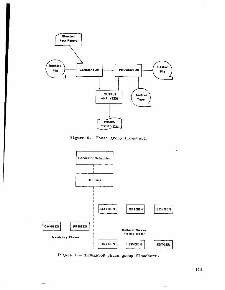
bul Record

\

F i g u r e 6 . - Phase group f lowchart .

I Generator Scheduler

I I I I

I I I I

F] I I

Mandatory Phases I

I

F i g u r e 7 .-. GENERATOR phase

I G P T G E N ~ I ZONGEN 1

Optional Phases (In any order)

group f lowchart .

113

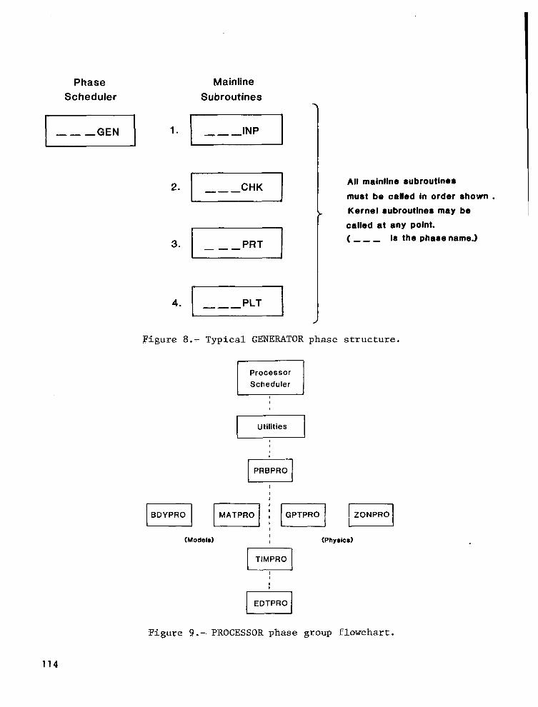
Phase Scheduler

Mainline Subroutines

3. r "- PRT 1 Ail mainline subroutine8

must be called in order shown . Kernel rubroutines may be

called at any Point. ( - - - ir the phase name.)

Figure 8.- Typical GENERATOR phase structure.

Processor

Utilities

I

I

EDTPRO

Figure 9.- PROCESSOR phase group flowchart.

114

SELF-ADAPTIVE INCREMENTAL

NEWTON-RAPHSON ALGORITHMS*

Joseph Padovan University of Akron Akron , Ohio 44325

SUMMARY

Multilevel self-adaptive Newton-Raphson type strategies are developed t o improve the solution efficiency of nonlinear f inite element simulations of s t a t i c a l l y loaded s t ructures . The overall strategy involves three basic levels. The f i r s t level involves preliminary solution "tunneling" via primative operators. Secondly, the solut ion is constant ly monitored via so-called quality/ convergence/nonlinearity tests. Lastly, the third level involves self-adaptive algorithmic update procedures aimed a t improving the convergence characteris- t i c s o f the Newton-Raphson s t ra tegy. Numerical experiments are included t o i l l u s t r a t e t he r e su l t s o f the procedure.

INTRODUCTION

Finite element ( F E ) or difference simulations o f continuum problems generally lead t o nonlinear modelling equations [1,2] . Generally, such simulations must be solved by va r ious techniques which are inherent ly i terat ive in nature . For instance, such methodologies as d i r ec t numerical integration, Newton-Raph- son ( N R ) , and modified Newton-Raphson ( M N R ) , as well as the incremental versions of such procedures (INR, IMNR) have a l l been employed [Z] . Since the types of nonlinearity exhibited by continuum problems are b o t h diverse and complex , the question of the best choice of an appropriate solution algorithm inevitably arises. Note, while many alternatives are available, generally the various solution procedures may have special advantages f o r cer ta in c lasses of problems b u t may exhibi t poor convergence for other s i tuat ions.

In this context, the ideal general purpose ( G P ) nonlinear FE code should have numerous algorithmic options augmented w i t h a degree of a r t i f i c i a l i n t e l - ligence. Namely, the problem solving capability should involve a heuris t i - ca l ly gu ided t r i a l and error search i n the space of possible solution via an automatically structured algorithm. Unfortunately, because of the inherent d i f f icu l t ies assoc ia ted w i t h code archi tecture and kinematic, kinetic, con- s t i t u t i v e and boundary conditior! formulations, generally only one algorithmic option i s usually available in GP codes. In this context, because of i t s wide

* T h i s work has been pa r t i a l ly supported by the ONR under Grant N00014-78-C- 0691 and by NASA under Grant NA63-54.

115

appl icabi l i ty , most GP nonlinear FE codes employ some v a r i a n t of either the s t ra ight o r modified INR a1 gorithmic procedures.

Note, while nonlinear codes present the user with f a r reaching capabilities, without a priori physical i n s i g h t , expensive parametric studies are oftentimes necessary to insure adequate s o l u t i o n convergence. For instance , unless the proper load increment i s employed, e i the r poor convergence or o u t of balance loads are generally encountered. Incorporating heuristic programming could eliminate some of the expensive and time consuming parametric studies t h a t are now required t o determine the proper incrementation necessary for reasonable convergence.

In view of the shortcomings of the current generation of solution algorithms, th i s paper will consider the development of self-adaptive NR s t r a - tegies for the solution of nonlinear FE or difference simulations o f s t a t i - cal ly loaded s t ructures . The main thrust will be to consider strategies which for the most p a r t are compatible with currently available GP codes. The over- a l l development will be considered in three main levels. The f i r s t will involve the use of INR operators t o "tunnel" into the solution space in the usual manner. The second level will involve the constant monitoring o f the different stages of solution via various qual i ty/convergence/nonl ineari ty t e s t s . Finally, the 1 as t l eve l i s an outgrowth of the findings of the second; namely, i f one or more o f the quality/convergence/nonlinearity tests are violated, various sce- narios are then triggered t o modify the INR strategy.

Based on the foregoing, the paper will outline in detail the multilevel static solution strategy, the development of the quality/convergence/nonlinea- r i t y t e s t s a s well as overview the various self-adaptive iterative update procedures. The analytical considerations will be complemented by several numerical experiments which outline the various aspects of the quality/convergence/ nonlinearity tests and which demonstrate the self-adaptive strategy.

MULTILEVEL SOLUTION STRATEGY:

OVERVIEW

As noted earlier, unless the proper load incrementation i s employed, e i ther poor convergence o r o u t of balance loads are generally encountered. Such anomalous behavior is generic t o all nonlinear codes employing non-self- adaptive INR a1 gorithms. In this context, the main thrust, of this work i s t o establish a three level iterative solution strategy involving:

i ) Level 1 ; Preliminary solution development via the primative b u t computational l y e f f i c i en t IMNR algorithm;

i i ) Level 2 ; Solution monitoring v i a qual ity/convergence/nonl ineari ty t e s t s and;

opera tor. i i i ) Level 3; Self-adaptive update procedures t o modify the primative

116

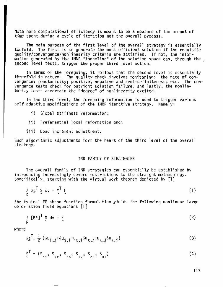
Note here computational efficiency i s meant to be a measure of the amount of time spent d u r i n g a cycle o f i t e ra t ion n o t the overall process.

The main purpose of the f i r s t l e v e l of the overall strategy is essentially twofold. The f i r s t i s to generate the most efficient solution if the requisite qual ity/convergence/nonl inear i ty cr i ter ia are sat isf ied. I f n o t , the information generated by the IMNR "tunneling" o f the solution space can, through the second level tests, tr igger the proper t h i r d level action.

In terms of the foregoing, i t follows that the second level i s essential ly threefold in nature. The quali ty check involves monitoring: the ra te of convergence; monotonicity; positive, negative and semi-definiteness; etc. The convergence t e s t s check for outr ight solut ion fa i lure , and lastly, the nonlinearity tests ascertain the "degree" of nonlinearity excited.

In the t h i r d level , the foregoing information i s used t o trigger various self-adaptive modifications of the IMNR i terat ive s t ra tegy. Namely:

i ) Global stiffness reformation;

i i ) Preferential local reformation a n d ;

i i i ) Load increment adjustment.

Such algorithmic adjustments form the heart of the third level of the overall strategy.

INR FAMILY OF STRATEGIES

The overall family of INR s t ra tegies can essent ia l ly be established by introducing increasingly severe restrictions t o the straight methodology. Specifically, start ing w i t h the virtual work theorem depicted by [ l ]

/ 6 g S d v = Y F R

T T - "

the typical FE shape function formulation yields the following nonlinear large deformation field equations [1]

J [B*IT S dv = F R - -

where 65 T- = - 1 (6Ui , j+6u j , i+u2 , i6U2 , j + u

2 2,jGu!2,,i 1

S T = ( S l l , S - 2 2 Y S 3 3 , s 12 Y S 2 3 Y S 3 1 1

117

such t h a t g , s, and ,F are, respectively, the s t ra in tensor i n vector form, the second Piola Kirchhoff pseudo s t ress t ensor , the nodal displacement vector, and l a s t l y , the nodal, force vector.

To sol ve ( 2 ) , the Taylor expansion theorem can be used t o establ ish the following tangent stiffness formulation, namely

where A& denotes the i th nodal displacement iterate associated with the Rth load increment. T h e nodal displacement, tangent st iffness and load imbalance are defined by

R

AFi = F - J [B*(Y! ) I T a ( v i - ) dv R R R - " R -1 - 1

such that Ik , [ O ( Y ~ - ~ ) ] , ED and F respectively denote the number of i t e ra t ions required of k t foad step, t h i i n i t i a l stress matrix, the tangent material st iffness and the total nodal load a f t e r R increments. For the s t ra i - g h t INR approach, [ K t ] i s continuously reformed and inverted. This is obviously quite expensive. In this context, the following versions of the INR a1 gor i - t h m can be established for a specific load increment solution cycle, namely:

R

i ) S t r a i g h t INR w i t h constant reformation of tangent stiffness matrix during i teration;

i i ) I n t e rmi t t en t global reformation during iteration;

i i i ) Preferent ia l local reformation during i terat ion;

i v ) BFGS type [3] reformation during iteration;

v ) Classical modified INR procedure wherein s t i f fnes s is reformed only a t beginning of load step;

v i ) No reformation, just i t e ra t ion ;

v i i ) Reformation with no i t e r a t ion , e t c .

As will be seen later, various versions of the foregoing INR family of algori thm are incorporated i n the self-adaptive strategy. This will obviously lead to a hierarchy w i t h varying degrees o f computation power/efficiency.

118

QUALITY/CONVERGENCE/NONLINEARITY TESTS

The quality/convergence/nonlinearity tests are the core of the m u l t i - level strategy. Such t e s t s a r e themselves organized i n t o three main categories, namely:

i ) C1 assical norm type convergence t e s t s ;

i i ) Qual i t y of convergence t e s t s and;

i i i ) Degree of nonlinearity tests.

The f i r s t group of tes ts are essent ia l ly of the normed type pass or fail vari- ety as typified by:

a ) The out of balance norm t e s t ;

b ) The global displacement norm t e s t ;

The main intent of such t e s t s i s e s sen t i a l ly t o monitor the success o r fa i lure of the iterative process. Note, while such tes t s a re e f f ic ien t and well adapted t o th i s purpose, they cannot be used effectively t o forecast potential d i f f icu l t ies un t i l o u t r i g h t failure occurs.

In this context, what i s required are so-called quality checks which enable a constant moni tor ing of the solution so as t o determine whether the direction of convergence i s proper. This i s the purpose of the second stage of checking. Namely, the quality checks t e s t whether the i terat ive process pos- sesses the requisite: rate; monotonicity; positive, negative and semi definiteness: e t c . Once determined, such information i s used t o trigger the various modifications of the primative f i r s t l e v e l IMNR strategy.

Since the paper i s mainly concerned w i t h s t a t i c loading problems, various statements concerning the quality of solution convergence can be made a t the outset. For instance, since most s t a t i c loading i s applied in a monotone fash- ion, i t i s expected t h a t unless there i s overshoot, successive iterated solutions should behave as a monotone, positive, negative or semi definite sequence. Behavior to the contrary obviously represents either overshoot or potential divergence.

Since i t is difficult to ascertain the monotonicity and definiteness from e i the r of the normed or vectorial versions of the nodal displacements and forces , a l ternat ive f ie ld measures must be employed. In this direct ion, the 1 oca1 (element) and global s t r a in energy stored can serve i n such a capacity. This follows from the f ac t t h a t fo r monotone loading situations, successive

119

I

I

i terations lead to a monotone posit ive definite sequence o f energy i t e r a t e s for softening structure. In the case of hardening s i tuat ions, successive i te- ra tes may be nonmonotone f o r a t l e a s t t h e f i rs t two iterates. Thereafter, the energy i te ra tes tend t o be monotone and negative definite. This process is c lear ly seen by the normed analogy of the i t e r a t ive process depicted i n Figures 1 and 2.

The incremental i t e r a t e energy stored d u r i n g a given iteration step is essentially the shaded area i l lustrated i n Figure 1 . Realizing t h a t the or- dinate values o f the true solution curve are given by (1 ) , i t fo l l ows that the incremental energy stored d u r i n g the k t h i t e ra t ion s tep o f the Rth load increment can be approximated by the following inner product, t h a t i s

Assuming tha t a to ta l o f KR i teration steps are associated w i t h the Rth loadstep, then the following expression can be developed for the energy stored, namely:

R K -1

k=l ' k = l (!k + !k+l) '!k+l

R K -1 E = C E:= R T R

Note ( 1 2 ) i s e s sen t i a l ly a trapezoidal type integration a proximation for the area under the hyper-curve defining the solution of the RtR loadstep. Now, sumning ( 1 2 ) over the ent i re set of L loadsteps associated w i t h a given problem yields the requisite overall strain energy stored,namely:

= 1 c ""I R R T R R=l k = l (!k + !k+l) '!k+l (13)

To obtain the strain energies for say the eth element, (13) must be inter- preted from a local point of view. Namely, the requisite parti t ions of Fke and Ayke must be employed i n a partitioned version of (1 3 ) , tha t i s

-

where here AYRe and _Fie, are respectively the local and element nodal displace- -

7 20

ments and forces. Note, due t o the form of (14) , any form of tangent stiffness type of consti tutive law can be accomodated.

In terms of the iteration process associated w i t h softening media, i t f o l - lows t h a t fo r convergent s i tuat ions

t h a t i s , successive i terates are monotone and posit ive definite. Hence, for softening media, a check of successive iterates for monotone decreasing pos i - t ive definiteness will establish a measure of the quality of convergence. For the hardening case , the E; sequence associated w i t h the convergent solution process takes the form:

E < E <.. .< E k < ... < O < E R R R R 2 3 1

As can be seen, f o r k>l, the sequence Ek i s monotone increasing b u t negative R

def ini te . In this context, similar t o the softening case, a check of the monotone increasing negative definiteness of successive i terates is used as one of the measures of the quality of convergence.

A l a s t b u t very important way of predicting potential solution difficul- t i e s can be achieved by moni toring the degree of nonl ineari ty excited as the deformation process continues. This can be achieved by selectively checking the changes of curvature of the global and local strain energy space. Such behavior can be ascertained using difference operators t o evaluate either the slope, rate of change of slope, o r more elaborately, the radius of curvature of the energy space as e i ther a function of the loading parameter or the nodal displacements. An a1 ternative approach would be t o locally spl ine f i t the energy-loading parameter space. In t h i s way, the current curvature/slope can be obtained either on a 1 oca1 el ement o r global basis. Such information can be used t o i n i t i a t e changes i n load step size as we1 1 as t o control local and global stiffness reformation.

The importance of such t e s t s follows from the f ac t t h a t a1 t h o u g h FE simulations of structures composed of general media undergoing large deflections are inherently nonlinear, the degree of nonlinearity excited varies from p o i n t t o p o i n t as well as from load increment t o load increment. As i t i s possible t h a t large por t ions of the structure may exhibit basically linear behavior, many general purpose codes a1 low the user t o p a r t i t i o n the overall structure i n t o i t s l i n e a r and nonlinear groups. A1 though this cer ta inly adds to the efficiency of the code, generally such information i s n o t known a priori unless extensive parametric studies have already been performed. In this context, the nonlinearity check will enable the automatic partitioning of the structure by allowing for preferential reformation of the tangent stiffness depending on the amount of local nonl ineari ty excited.

121

ADAPTIVE STRATEGY

In the context of the inherent features o f the INR family of algorithms, the adaptive strategy incorporates the following procedural options namely:

i ) Tangent stiffness reformation and;

i i ) Load increment adjustment.

Each of these options in turn involves several different levels. For instance, stiffness reformation can be considered i n several stages, t h a t i s :

i ) Global reformation;

i i ) Preferential local reformation or;

i i i ) BFGS [3] reformation.

The adaptive incremental load can also be achieved in several ways namely:

i ) Increment expansion;

i i ) Increment contraction o r ;

i i i ) Corrective incrementation.

As noted ear l ie r , the in i t ia t ion of e i the r o p t i o n i s dependent on three basic c r i t e r i a , t h a t i s :

a ) Qual i ty of convergence;

b ) Outright failure to converge o r ;

c ) The degree of nonl i neari ty excited.

While the reformation o p t i o n is t r iggered by the second level tests, the specific adaption triggered is primarily dependent on the degree of nonlinear- i ty excited. Hence, for mildly nonlinear (elastic) si tuations, the BFGS reformation process i s employed. In the case where significant local o r global non- l inear i ty i s excited, then either global o r preferential reformation is ini- t ia ted.

As can be seen from the proceeding categories, various types of load crementation are possible. The overall strategy i s a combination of such

i n -

options. Specifically, when significant solution degradation is monitored by the level two t e s t s , then corrective incrementation i s i n i t i a t ed . Namely, negative load incrementation i s employed t o enable the retracing of a portion of load history wherein a lower order algorithmic strategy yielded poorly converged resul ts.

To s t r ike a balance between solution convergence and economy, the overall

1 22

adaptive strategy i s centered a b o u t a primative version of the INR algorithm namely the IMNR. Depending on the results of the qual ity/convergence/nonl inea- r i ty tes ts , the level of the IMNR is e i ther upgraded o r lowered by modifying the pattern of stiffness reformation and incrementation. Note, since the main incentive is t o achieve a successful solution a t least cost , the hierarchy is ordered t o f i r s t implement increment adjustment and then reformation. As a further move to achieve economy, the global reformation process typically employed a t t he s t a r t of an IMNR increment can be established preferentially depending on the curvature tolerance associated with the global and local non- 1 ineari ty checks.

Since space is limited, a full description of the various detailed hier- achies must be lef t to future publ icat ions. In this context, for the present purposes, Figure 3 gives a good overview of all the possible flows o f control associated with the three-level strategy. As can be seen from this f igure, contingent upon the various "flags" generated in the level two tes ts , the condition code check routine will initiate the actual modification of the INR strategy a l o n g the lines outlined i n the proceeding discussion.

DISCUSSION

Interestingly, while such factors as geometry, material properties, boundary condi t ions, e tc . , a l l have some ef fec t on the choice of load increment s ize , once an excessive value has been chosen, typically similar types of solution degradation are encountered when only the primative non-self-adaptive algorithm i s used. Specifically, three basic types of solution pathology tend t o occur. These can be categorized by:

i ) Immediate and strong nonmonotonicity;

i i ) Moderate b u t progressively increasing nonmonotonicity and nonpositive definiteness and;

i i i ) Mild monotonicity with e i ther very gradual increases o r decreases i n solution oscil lation.

Note, such behavior can be excited either in the f irst o r successive load steps. Figures 4 and 5 give examples of such behavior. While the resul ts i l lust rated pertain t o a rubber sheet, similar results were obtained for e las t ic /plast ic media as well as for different geometries and boundary conditions.

The solution failure depicted i n Figure 5 is typical of those that usually arise. Specifically, as can be seen, for the given load increment excellent convergence is obtained i n t he f i r s t s t ep . In the second, a mild form of nonmonotonicity and nonpositive definiteness is encountered. Finally, i n the t h i r d step, strong and progressively increasing nonpositive definiteness is encountered. Solution failure i s f i n a l l y i n i t i a t e d by out of balance loads. T h i s scenario is typical of excessive load incrementation. Note, a s can be seen from these results; the onset o f such behavior i s signalled by the i n i - t i a t ion of nonmonotonicity or incorrect definiteness. By studying the behavior

1 23

I '

of local element energies, additional insights are obtained. For the problems illustrated in Figures 4 and 5 , the solution degradation is in i t ia l ly loca- l ized b u t gradually spreads to the entire structure as the iteration process continues. Employing the self-adaptive strategy to the foregoing problems caused the second level monotonicity t e s t s t o trigger automatic increment adjustment and preferential stiffness reformation. T h i s led t o the generation of the correct solution. The overall strategy was tested on several nonlinear problems which exhibited pathological behavior for given load increment choices. The types o f problems considered combined varying degrees o f kinematic, kinetic and material nonlinearity. In each case barring possible bifurcations, the level two t e s t s were able to automatically initiate the requisite corrective self adaptions t o enable successful solutions. The .main problem encountered with the concept of self-adaptive strategies arises from the fact t h a t some engineering insight must be practiced in order to cut down overall running times. Otherwise, excessive execution times are encountered a s the adaptive strategy shifts gears t o adjust for improper incrementation.

R E F E R E N C E S

1 . Zienkiewicz, 0. C. , "The Finite Element Method", McGraw Hill Co. New York, 1978.

2. Chang, T . Y. and Padovan, J . , "General Purpose Fini te Element Programs," Structural Mechanics Software Series, Vol. 111, Nicholas Parrone and Walter D . Pilkey, eds., Univ. Press o f Va., 1980.

3. S t r a n g , G . , "Numerical Computations in Nonlinear Mechanics", ASME Paper No. 79-PVP-114.

124

f

Fe-

r: r: rS r: 1 +

" e - 1

Figure 1.- I t e r a t

f

ICE NOW

D I SPLACEFENT NORM

ion process f o r hardening prob

- DISPLACEENT NORM

1 em.

Figure 2.- Iteration process for softening problem.

125

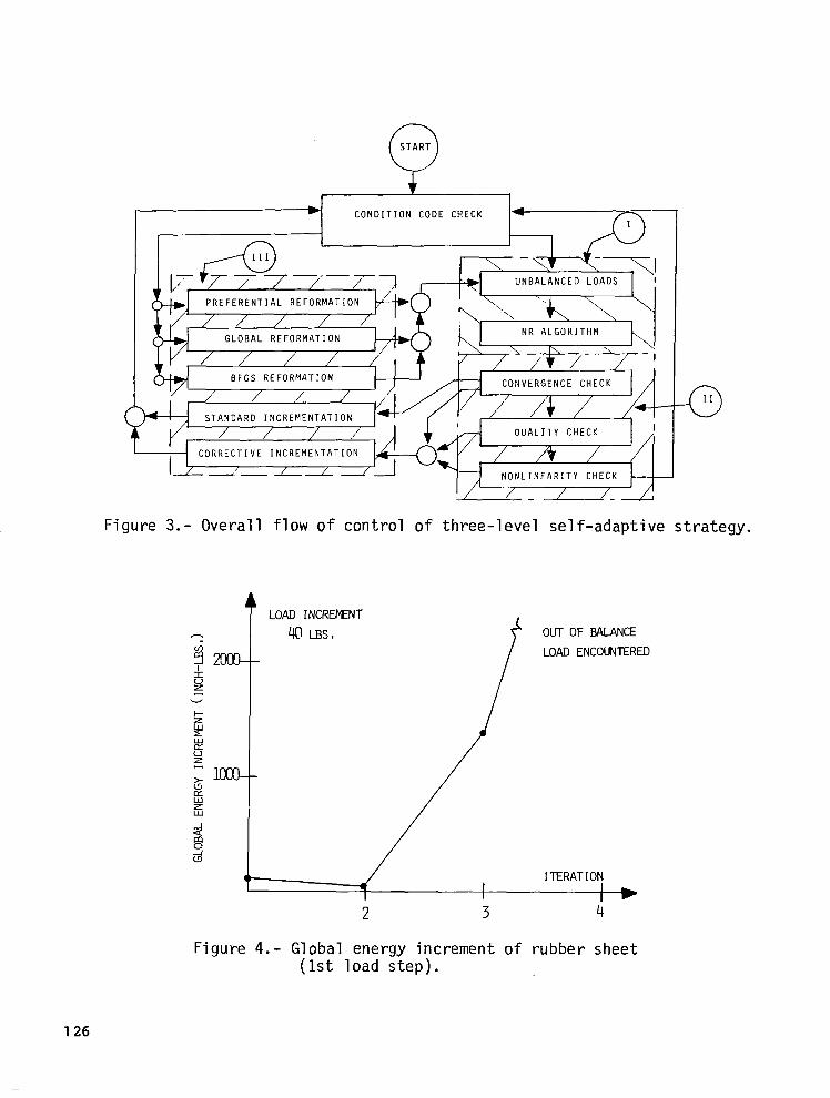
(7 S T A R T

* C O N D I T I O N C O D E C H E C K

U N B A L A N C E D L O A D S

P R E F E R E N T I A L R E F O R M A T I O N

N R A L G O R I T H M

C O N V E R G E N C E C H E C K

S T A N D A R D I N C R E M E N T A T I O N Q U A L I T Y C H E C K

C O R R E C T I V E I N C R E M E N T A T I O N

-0

Figure 3.- Overall flow o f control of three-level self-adaptive strategy.

f LOAD INCREMENT OUT OF BALANCE

LOAD ENCOUNTERED

t ITERATION I

I I ) 2 3 4

Figure 4.- Global energy increment of rubber sheet (1s t load s tep) .

1 26

I . 1ST LOAD STEP

OUT OF BALANCE

Figure 5.- Global energy incremer,t o f rubber sheet ( l s t , Znd, 3rd load s teps) .

127

,, , I .. . . . ... . . . .- ”

STUDY OF SOLUTION PROCEDURES FOR NONLINEAR

STRUCTURAL EQUATIONS

Cline T. Young I1 Mechanical and Aerospace Engineering

Oklahoma State University

Rembert F. Jones, Jr. David Taylor Naval Ship R & D Center

SUMMARY

A method for the reduction of the cost of solution of large nonlinear structural equations was developed. Verification was made using the ITARC-STRUC structure finite element program with test cases involving single and multiple degrees-of-freedom for static geometric nonlinearities. The method developed was designed to exist within the envelope of accuracy and convergence characteristic of the particular finite element methodology used.

INTRODUCTION

At present the finite element codes in conjunction with the large, high- speed computers available are capable of producing reasonable solutions to practically all static problems conceivable in structural analysis. In addition, well-behaved problems such as those involving small elastic deformations are solved relatively inexpensively and accurately. Computational difficulties do not arise until the stiffness of the structure becomes a function of displacement and/or displacement history. An opinion widely held is that when this does occur an implicit solution scheme is necessary for accuracy. All implicit schemes require an iterative solution where there is an attempt to reduce some error term to zero at each iteration. Therefore, a nonlinear problem is more expensive to solve and can become astronomically so depending upon the degree of nonlinearity and the convergence criteria used.

In the solution of nonlinear structural equations the reformulation of the stiffness matrix is a first order contribution to the cost. The first logical step in attempting to reduce the cost would be to seek a less expensive way to update the stiffness matrix. This of course has been done with some success and i9.appare.ntl.y still being researched. Looking at only the most recent developments or evaluations we see that Mondkar and Powell [l] have used the constant alpha technique to try updating the stiffness matrix for the modified Newton-Raphson approach. Matthies and Strang [2,,3] have taken similar approaches born from a paper by Dennis and More [ 4 ] on Quasi-Newton methods. The basic premise was that the stiffness matrix could be updated without going through the full process of reformulation and decomposition or inversion. The most popular approach was to update the stiff-

1 29

ness matrix by a mat r ix o f rank two. Th i s is known as t h e BFGS (Broyden- Fletcher-Goldfarb-Shanno) u p d a t e . C r i s f i e l d [5] used a method similar t o a BFGS update of rank one. A l l of t hese pape r s show conclus ive ev idence of c o s t r e d u c t i o n f o r c e r t a i n p r o b l e m s . The las t by C r i s f i e l d is c l o s e s t i n f o r m t o t h e method developed here.

A s e c o n d l o g i c a l s t e p is t o r e d u c e t h e number of i t e r a t i o n s r e q u i r e d t o s a t i s f y t h e c o n v e r g e n c e cri teria. This can be done by determining an estimated displacement as a c c u r a t e l y as p o s s i b l e . The development which follows shows how t o do t h i s . A l l f o r c e s and loads are of an incrementa l na ture .

DEVELOPMENT

I n g e n e r a l , t h e i t e r a t i v e m e t h o d s of s o l u t i o n u s i n g t h e s t i f f n e s s f o r m u l a - t i o n w i l l by some l o g i c a l means c a l c u l a t e a gene ra l i zed d i sp l acemen t fo r a g iven gene ra l i zed l oad . Re tu rn ing t hen t o t he e l emen ta l l eve l , t he e l emen ta l s t i f f n e s s matrices are a l t e r e d t o r e f l e c t t h i s c h a n g e i n s h a p e and t h e t o t a l r e s i s t a n c e of t h e s t r u c t u r e t o t h e a p p l i e d l o a d i s d e t e r m i n e d . I f t h e s t r u c - t u r e i s to be cons ide red i n equ i l ib r ium, t he app l i ed l oad mus t be exac t ly balanced by t h e r e s u l t i n g r e s i s t a n c e of t h e s t r u c t u r e . Any imbalance i s termed a r e s i d u a l f o r c e and must be considered as a n e r r o r . An a t t e m p t i s made t o r e d u c e t h i s e r r o r by a l t e r i n g t h e e s t i m a t e d d i s p l a c e m e n t . The r a t e of convergence depends on the manner of es t imated displacement select ion.

The v a s t m a j o r i t y of i m p l i c i t s c h e m e s a v a i l a b l e u t i l i z e o n l y t h e m o s t r ecen t r e s idua l and t he reby i gnore any poss ib l e t r end de t e rmina t ion . Fe l ippa [ 6 ] recognized th i s and proposed a v i a b l e method f o r d e t e r m i n i n g t h e d i s p l a c e - ment t h a t would y i e l d t h e least r e s i d u a l w i t h i n s p e c i f i e d l i m i t a t i o n s . T h i s approach requi red the de te rmina t ion of a w e i g h t i n g m a t r i x t h a t w a s dependent upon the e lements chosen and the appl ied loads. The development i n t h i s pape r is independent of t h e p h y s i c a l c h a r a c t e r i s t i c s of the e lements .

A key element i n t h e s u c c e s s of the approach developed i s t h e f i n i t e element method used. A s ment ioned before the MARC-STRUC s t ruc tu re p rog ram was u s e d b u t t h e v a r i a t i o n a l f o r m u l a t i o n of t h e s t r u c t u r a l e q u a t i o n s w a s performed a c c o r d i n g t o t h e method of Jones [7 ] . It i s most important to have the most a c c u r a t e method p o s s i b l e f o r t h e d e t e r m i n a t i o n of t h e r e s i d u a l s .

Cons ide r ing t he so lu t ion fo rm, i n F igu re 1 a graph of f o r c e v e r s u s d i s - placement is shown. The c u r v e r e p r e s e n t s t h e c a l c u l a t e d r e s i s t a n c e of t h e s t r u c t u r e . The o r i g i n a l s t i f f n e s s m a t r i x , Roy a s s u m e s l i n e a r l y e las t ic de fo r - mat ion and y ie lds the d i sp lacement , uo , and t h e r e s i d u a l , Ro, f o r t h e a p p l i e d load , F. The displacement , uo , and r e s i d u a l , Ro ,-are t h e n u s e d i n a Quasi- Newton f a s h i o n t o u p d a t e t h e s t i f f n e s s m a t r i x t o K 1 and a new disp lacement , i1, and consequently a new r e s i d u a l , R i , are ca lcu la ted . Highly accura te answers may r e s u l t , b u t t h e y are c l e a r l y e x p e n s i v e t o o b t a i n .

- - - -

-

The e x t r a p o l a t i o n method presented i n t h i s p a p e r i s c l e a r l y e x e m p l i f i e d by t h e t r i a n g l e , ACE, shown i n F i g u r e 2. The method used w a s i d e n t i c a l t o t h e d i r e c t i t e r a t i o n method (shown i n F i g u r e 1 e a r l i e r ) up t o and through the

130

c a l c u l a t i o n of uo, R, and ul, R1. It w a s t he de t e rmina t ion o f t he new estimated displacement, 9 , t h a t w a s p e r f o r m e d d i f f e r e n t l y . I n a one dimensional s e n s e t h e r e s i d u a l s Roy K 1 and the dis tance between them, a, were u s e d t o c a l c u l a t e a scalar, w, t h a t p r e d i c t e d t h e d i s p l a c e m e n t a t which equi l ibr ium supposed ly ex i s t ed unde r t he l oad , F. Of c o u r s e , t h i s w a s n o t t h e e q u i l i b r i u m p o s i t i o n and a new r e s i d u a l , _R2,-was determined. The r e s i d u a l s , El, E2 , and the dis tance between them, wd - d , were t h e n u s e d t o p r e d i c t a new equ i l ib r ium p o s i t i o n . The p rocess con t inued un t i l conve rgence w a s s a t i s f i e d .

- - " -

- -

A major d i f f i cu l ty encoun te red w a s t he de t e rmina t ion of t h e scalar, W. I n a one dimensional case it w a s easy enough to see t h a t

However, s i n c e i n g e n e r a l t h e v e c t o r s Eo, El and d are h e t e r o g e n e o u s i n t h e i r components ' uni ts , a d i v i s i o n as mentioned above i s impossible even when u s i n g vec to r l eng ths . The s o l u t i o n t o t h i s d i f f i c u l t y came about by c o n s i d e r i n g t h e u n i t s of work. I n f a c t , t h i s e x t r a p o l a t i o n p r o c e s s may be symbol ica l ly thought of as minimizing the work done by t h e r e s i d u a l s . I n t h i s l i g h t i t w a s t hen dec ided t ha t equa t ing t he area of t h e t r a p e z o i d , ABDE, p l u s t h e area of t h e t r i a n g l e , BCD, t o t h e area of t h e t r i a n g l e , ACE, would r e s u l t i n a n e q u a t i o n with only one unknown. Simplifying and rearranging, the fol lowing w a s ob ta ined .

- - Ro d

w = - (Eo-R1) d

A t t h i s p o i n t i t w a s decided to implement the theory and test f o r a one degree- of-freedom case and fol low that wi th a more complex case .

VERIFICATION

I n a n a t t e m p t t o d e t e r m i n e t h e v a l i d i t y of the a forement ioned ex t rapola- t i o n method i t w a s de t e rmined t ha t a one dimensional buckling problem would be a p p r o p r i a t e as a f i r s t t es t case. The bar-spring problem of Jones w a s s e l e c t e d .

Bar-Spring Problem

I n F i g u r e 3 the dimensions used on the problem may c l e a r l y b e s e e n . The l e n g t h of t h e s p r i n g w a s unimportant as long as n o n l i n e a r e f f e c t s d i d n o t e n t e r t h e c a l c u l a t i o n s f o r t h e s p r i n g ' s d e f l e c t i o n . The b a r w a s modeled s o as t o a l low only a change i n l e n g t h and no bending deformation, hence the absence of an E 1 t e r m . A load w a s a p p l i e d a t t h e end of t h e b a r and s p r i n g i n t h e d i r e c - t i o n of de fo rma t ion t o r ende r t he p rob lem one of a pu re ly s ing le d imens iona l

1 31

case. The buck l ing l oad was a t 2.7 kg. ( 6 l b . ) w i t h t h e r e s u l t s t a b u l a r i z e d i n T a b l e I. The exact deformat ion w a s c a l c u l a t e d a n d p l o t t e d i n F i g u r e 4 t o show t h e h i g h d e g r e e of nonl inear i ty o f the p roblem.

I n a n a l y z i n g t h e r e s u l t s (see Table I) i t w a s d e c i d e d t h a t a comparison of the v a l u e s c a l c u l a t e d a g a i n s t t h e exact v a l u e s as w e l l as a comparison of the number of i t e r a t i o n s r e q u i r e d f o r e a c h method would be of use. The r a i s e d numbers b e s i d e t h e c a l c u l a t e d d i s p l a c e m e n t s i n T a b l e I r e p r e s e n t t h e number of i t e r a t i o n s r e q u i r e d a b o v e t h e o r i g i n a l estimate t o r e d u c e t h e q u o t i e n t of t h e ca l cu la t ed d i sp l acemen t and t he e s t ima ted d i sp l acemen t t o t he t o l e rance i nd i - ca t ed a t t h e column heading.

It shou ld be no ted t ha t a t t h e b u c k l i n g l o a d t h e t o l e r a n c e r e q u i r e d t o o b t a i n two s i g n i f i c a n t d i g i t s a c c u r a c y , 1 . 0 0 1 , l e d t o a 5 v s . 26 advan tage i n i t e r a t i o n s f o r t h e new method. However, t h e new method w a s edged by t h e o l d in the pos t -buckled reg ion by a c o n s i s t e n t 4 v s . 7 margin . The reason for th i s w a s a p p a r e n t l y t h a t t h e l i n e a r e x t r a p o l a t i o n d i d n o t f o l l o w t h e c h a n g i n g s t i f f - nes s of t h e s t r u c t u r e v e r y w e l l . I f so , a b e t t e r a p p r o x i m a t i o n would be obta ined wi th a p a r a b o l i c e x t r a p o l a t i o n .

On t h e w h o l e t h i s e x t r a p o l a t i o n showed promise i n t h i s c a s e b u t n o t of a c l e a r l y d e c i s i v e n a t u r e . T h e r e f o r e , t h e m o t i v a t i o n f o r a more complex example was e s t a b l i s h e d .

Ring Buckling Problem

This problem w a s t o d e t e r m i n e t h e d e f l e c t i o n o f a r ing unde r a uniformly l o a d e d e x t e r n a l p r e s s u r e of v a r y i n g v a l u e s . The r i n g w a s modeled through 90 degrees as shown i n F i g u r e 5. The 90 degree a r ch w a s b roken i n to two subs t ruc - t u r e . The degrees of freedom per node were

1. z 2 . R 3 . dZ/ds 4 . dR/ds

w i t h t h e r o t a t i o n s p o s i t i v e as shown by 0 i n F i g u r e 5. The r i n g was modeled w i t h a modulus of e l a s t i c i t y of 2 . 1 x l o 6 kg/cm2 ( 3 0 x 106 psi) and a r a d i u s of 51 cm ( 2 0 i n . ) . F i n a l l y , a k i c k e r f o r c e w a s a p p l i e d a t node 1 of subs t ruc - t u r e 1 i n t h e n e g a t i v e R d i r e c t i o n w i t h a magnitude of 1 .5 x kg. (3 .4 x 10-6 l b ) . Obvious ly , th i s w a s s i m p l y t o f o r c e t h e r i n g i n t o a buckled mode w i t h o u t a l t e r i n g t h e d e f l e c t i o n s d u e t o t h e p r e s s u r e l o a d i n g .

As t h e r e w a s no e x a c t s o l u t i o n o t h e r t h a n t h e known c o l l a p s e l o a d , t h e tolerance chosen, 1 .001, w a s t h a t which gave two s i g n i f i c a n t d i g i t s a c c u r a c y for the bar -spr ing problem. The r e su l t s obta ined are shown i n T a b l e 11. The p o i n t a t which. t h e s t r u c t u r e would "collapse" w a s 4.22 kg/cm2 (60 p s i ) . A s can b e s e e n , t h e r e s u l t s were qui te remarkable as t h e s t r u c t u r e became s o f t e r . A t 4.18 kg/cm2 (59.5 p s i ) t h e number of i t e r a t i o n s r e a c h e d by t h e o l d method were n o t e n o u g h y e t t o s a t i s f y t h e t o l e r a n c e r e q u i r e m e n t o f 1.001. The authors s u s p e c t t h a t a n o t h e r 50 t o 100 i t e r a t i o n s would have been required.

132

CONCLUDING

t h i s p a p e r

REMARKS

w a s t h e c o s t of s o l u t i o n o f l a r g e n o n l i n e a r s t r u c t u r a l e q u a t i o n s . T h i s d i f f i c u l t y h a s b e e n and i s be ing r e sea rched ; however , t he d i r ec t ion of most p resent research i s a p p a r e n t l y con- c e r n e d w i t h t h e s e c o n d p a r t i a l of t h e s t r a i n e n e r g y e x p r e s s i o n ( s t i f f n e s s matr ix) . This paper implies and subsequent research by t h e a u t h o r s s u p p o r t s t h e s u p p o s i t i o n t h a t t h e f i r s t p a r t i a l of t h e s t r a i n e n e r g y e x p r e s s i o n ( r e s i s t - i n g f o r c e ) i s n o t b e i n g f u l l y u t i l i z e d i n t h e d e t e r m i n a t i o n of t h e new estimated displacement needed f o r impl ic i t methods . It may w e l l b e d e t e r m i n e d t h a t updat ing and/or re formula t ion of t h e s t i f f n e s s m a t r i x is o c c u r r i n g f a r t o o o f t e n i n p r e s e n t s o l u t i o n t e c h n i q u e s .

133

REFERENCES

1. Mondkar D. P. and G. H. Powell, "Evaluation of Solution Schemes for Non- linear Structures." Computers & Structures, Vol. 9, 1978, pp. 223-236.

2. Matthies, H. and G. Strang, "The Solution of Nonlinear Finite Element Equa- tions." International Journal for Numerical Methods in Engineering, V O ~ . 14, pp. 1613-1626, Nov., 1979.

3 . Strang, G. and H. Matthies, "Numerical Computations in Nonlinear Mechanics." NSF Report, MCS 78-12363.

4 . Dennis, J. E. and J. J. More: "Quasi-Newton Methods, Motivation and Theory." SIAM Review, Vol. 19, pp. 46-89, 1977.

5. Crisfield, M. A., "A Faster Modified Newton-Raphson Iteration." Computer Methods in Applied Mechanics and Engineering, Vol. 20, pp. 267-278, 1979.

6 . Felippa, C. A., "Procedures for Computer Analysis of Large Nonlinear Struc- tural Systems." Large Engineering Systems, ed. by A. Wexler, Pergamon Press, London, pp. 60-101, 1976.

7. Jones, R. F., "Incremental Analysis of Nonlinear Structural Mechanics Prob- lems with Applications to General Shell Structures." Naval Ship Research and Development Center Report 4142, 1973.

1 34

TABLE 1

BAR-SPRING PROBLEM

Load

( lb ) Method ( 4 1.1 1.01 1.001 1.0001 1.00001 kg Exact

1.4 Old 0.59781 0.5915; 0. 59643 0.59785 4 0. 59786 €I 0.59787 7

(3.0 New 0.5915 0.5964 0.5978 0.5978 0.5978

2.7 Old 2.5400 2.01772 2.45454 l3 2.53205 2. 53926 39 2.54006 (6.0) New 2.2329 2.5018 2.5373 2.5400 2.5400

4.1 Old 4.4821 4 . 49331 4.48061 4.48211 (9.0) New 4.4788 4.4816 4.4821 4 .4821 4.4821

4

26 51

1 4 . 48211 4.48213. 1

5.4 Old 5.0800 5. 07923 5.08005 5.08007 5. 08008 5.08009 5

(12.0) New 5.0828 5.0803 5.0800 5.0800 5.0800 ~~

6.8 Old 5.4907 5. 49431 5.49075 5.49077 5. 49079 5.490710 4 6

(15.0) New 5.4948 5.4910 5.4907 5.4907 5.4907

8.2 Old 5.8143 5. 81761 5.81465 5.81437 5. 81439 5.814311 4 7

(18.0) New 5.8176 5.8148 5.8146 5.8143 5.8143

*Buckling Load

Note: When the number of i t e r a t i o n s is less than (2) , there i s NO di f fe rence between t h e new and old methods.

TABLE I1

RING PROBLEM (1,001)

Load Substructure 1 (cm) Substructure 2 (cm) kg 1 cm2 Node 1 Node 1 (psi) Method Iterations D.O.F. 2 D.O.F. 2

.5 Old ( 7 ) New

2 4

- .78547 E-03 -.41397 E-03 -.78555 E-03 -.41397 E-03

1 .5 Old 5 -.25537 E-02 - . l o 4 6 8 E-02 ( 2 1 ) New 4 - .25545 E-02 - . l o 4 5 9 E-02

2 . 5 Old 9 - .49439 E-02 - . l o 6 0 7 E-02 ( 3 5 ) New 4 - .49472 E-02 - . lo576 E-02

3 . 5 Old 23 - . lo230 E-01 .18 1 7 2 E-02 ( 4 9 ) New 3 - . lo237 E-01 , 1 8 2 4 3 E-G2

3 . 9 Old 5 4 ( 5 6 ) New 3

~~ ~~

- . 22451 E-01 .12827 E-01 -.22597 E-01 .12972 E-01

4 . 2 Old 149* -. 88354 E-01,k . 77978 E-Ol* (59 .5 ) New 4 -.95669 E-01 .85268 E-01

*Maximum number of iterations allowed. Convergence not yet satisfied.

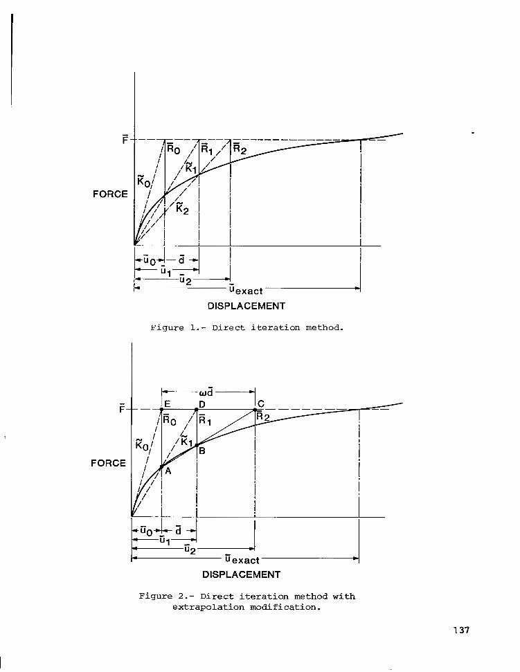
DISPLACEMENT

F- -

FORCE

Figure 1.- D i r e c t i t e r a t i o n method.

DISPLACEMENT

Figure 2.- D i r e c t i t e r a t i o n method with e x t r a p o l a t i o n m o d i f i c a t i o n .

137

7- 2.54 cm (1 in.)

P

$ A€ = 7.03 X IO5 kglcm2 ( IO7 psi) Q Q $

2 \ Ks = 1.07 kg/cm + (6 Iblin.) ? 2 ?

\

\ \

\ -

Figure 3. - Bar-spring problem.

DISPLACEMENT (in.) 0 0.5 1 .o 1.5 2.0 2.5

10.0 I I I I

- 20

7.5 - - 15

5.0- (kg) -10

n w

-5

I I

3.0 4.5 6.0 I -0

I

LOAD (Ib)

DISPLACEMENT (cm)

Figure 4.- E x a c t s o l u t i o n t o bar-spr ing problem.

1 38

2

Figure 5.- Ring problem.

1 39

.. . . ""

RESPONSE OF NONLINEAR PANELS TO RANDOM LOADS*

Chuh Mei Old Dominion University

SUMMARY

Lightweight aircraft structures exposed to a high intensity noise environment can fatigue fail prematurely if adequate consideration is not given to the problem. Design methods and design criteria for sonic fatigue prevention have been developed based on analytical and experimental techniques. Most of the analytical work was based upon small deflection or linear structural theory which did not agree with the experimental results. A large deflection geometrical nonlinearity was incorporated into the analysis methods for determining the structural response to high intensity noise. The Karman-Herrmann large deflection equations with a single-mode Galerkin approximation, and the method of equivalent linearization were used to predict mean-square amplitude, mean- square stresses, and nonlinear frequency at various acoustic loadings for rectangular panels. Both simply supported and clamped support conditions with immovable or movable inplane edges are considered. Comparisons with experimental results are presented.

INTRODUCTION

Vibrations caused by acoustic pressure can frequently disturb the operating conditions of various instruments and systems, and sonic fatigue failures which occurred in aircraft structural components cause large maintenance and inspection burdens. The development of sonic fatigue data and design techniques were initiated to prevent sonic fatigue failures. Design methods and design criteria for many types of aircraft structures have been developed under Air Force sponsorship and by the industry in the past twenty years. Reference 1 has a complete list of the reports describing these efforts. This research led to sonic fatigue design criteria and design charts which are widely used during the design of an aircraft. Although current analytical sonic fatigue design methods are essentially based on small deflection 01: linear structural theory (see ref. 1, page 209), many documented tests (refs. 2 - 6) on various aircraft panels have indicated that high noise levels in excess of 110 decibels (dB) produce nonlinear behavior with large amplitudes of one to two times the

*This work was supported by the Air Force Office of Scientific Research (AFSC), United States Air Force, under contract F49620-79-C00169.

1 41

I I I l l I II

panel thickness in such structural panels. The neglect of such large deflection geometrical nonlinearity in analysis and design formulations has been identified as one of the major causes for poor agreement between experimental data and analytical results. The evidence of those researchers was summarized in reference 7, where a comprehensive review of existing analytical methods on random excitations of nonlinear systems was also given.

In this paper, the Karman-Herrmann large deflection equations for rectangular plates (ref. 8) are employed. Using a single-mode Galerkin’s approximation, the dynamic equations reduce to a nonlinear differential equation with time as the indeFendent variable. The method of equivalent linearization (refs. 9 - 11) is then applied to reduce the nonlinear equation to an equivalent linear one. Mean-square displacements, mean-square stresses, and nonlinear frequencies at various acoustic loadings are obtained for rectangular panels of different aspect ratios and darnping factors. Both simply supported and clamped boundary conditions with immovable or movable inplane edges are considered. Comparisons with experimental results are also presented.

SYMBOLS

Panel length and width Panel dimension parameters, 27r/a and 2~/b Constants Bending rigidity Error of linearization Young ’ s modulus Equivalent linear frequency in Hz Stress function Panel thickness Frequency response function Spectrum level Mass coefficient Membrane stress resultant Constant Pressure loading Generalized or modal displacement Aspect ratio, a/b Spectral density function of excitation pressure p(t) Time Displacement of midplane Transverse deflection Coordinates Nonlinearity coefficient Nondimensional nonlinearity coefficient Ratio of damping to critical damping Nondimensional frequency parameter Poisson’s ratio Panel mass density Normal and shear stresses

I

w Radian frequency R Equivalent linear or nonlinear radian frequency Subscripts: b Bending C Complementary solution or critical m Membrane M X Maximum 0 Linear P Particular solution

FORMULATIOK AND SOLUTION PROCEDURE

Governing Equations

Assuming that the effect of both the inplane and rotatory inertia forces can be neglected, the dynamic von Karman equations of a rectangular isotropic plate undergoing moderately large deflections are (refs. 8 , 12):

v4F = E (.W2, - XY w'xx w,yy 1

where w is the transverse deflection of the plate, h is the panel thickness, p is the mass density of the panel material, D = En3/12 (1-V2) is the flexural rigidity, E is Young's modulus, V is Poissorr's ratio, p(t) is the exciting pressure, and a comma preceding a subscript(s) indicates partial differentiation ( s ) . The stress function F is defined by

( 5 = X F'YY

(5 = F, Y xx

where Ox, Oy, and T are membrane stresses. X y

Simply Supported Panels. For a rectangular plate simply supported along all four edges as shown in Figure 1, Chu and Herrmann (ref. 81, and Lin (ref. 13) have considered that if the fundamental mode is predominant, the motion of the panel can be represented adequately as

w = q (t) h cos (Trx/a) cos (Try/b) (4 1

where q(t) is a function of time only. The maximum value of q(t) coincides with

143

I

t h e maximum d e f l e c t i o n wmax d iv ided by p a n e l t h i c k n e s s h. The expres s ion w satisfies the boundary condi t ions for simple s u p p o r t s

w = w , + V W I = 0, on x = f a/2

w = w, + v w , ~ = 0, on y = f b/2

xx YY

YY

S u b s t i t u t i n g t h e e x p r e s s i o n f o r w i n Eq. ( 2 ) a n d s o l v i n g f o r a p a r t i c u l a r s o l u t i o n Fp y i e l d s

where r = a b . The complementary so lu t ion to eq l ia t ion ( 2 ) is t a k e n i n t h e form

where the cons tan ts Ex and Ny c o n t r i b u t e t o t h e membrane stresses Ox and Oy and are to be determined f rom the inplane boundary, immovable or movable , cond i t ions .

-

For t he immovable edges case, t h e c o n d i t i o n s o f z e r o i n p l a n e n o r m a l d i s - placement a t a l l four edges are s a t i s f i e d i n a n a v e r a g e d manner as

- V F , = ) - Ji w ~ , ~ ] dxdy, on x = f a / 2

where u and v are inplane d i sp lacements . For the movable edges case, the edges are f r e e t o move as a r i g i d body w i t h t h e a v e r a g e i n p l a n e stress equa l t o zero. The inp lane boundary condi t ions are

u = c o n s t a n t

v = cons tan t

on x = * a/2

on y = k b/2

where Nx and Ny are membrane stress r e s u l t a n t s p e r u n i t l e n g t h i n plate. By

1 4 4

making use of these inplane edge boundary conditions, equations (8) and (91, it easily can be shown that for the immovable edges

- Nx -

- q2h2ElT2

- q2h2ET2 (1 + vr2) 8a2 C1-v2)

N = tr2 + v) 8a2 C1-v2)

and for the movable edges - - N x = N = O

Y

the complete stress function is then given by F = F + Fc. P

With the assumed w given by equation (4) and stress function given by equations (6) and (71, equation (1) is satisfied by applying Galerkin's method

L(w,F) w dxdy = 0

from which yields the modal equation of the form

and

w 2 = x o - 2 D 0 phb4 r2

m = 'rr2ph2/16

B = B + B c = (B +Bc)- P P phb4

* * D

with

which satisfies the clamped support conditions

w = w, = 0, X

w = w, = 0 , Y

on x = f a/2

on y = k b/2

By introducing equation (15) in equation (2) and solving it, the particular stress function is

- q2h2Er2 [cos Ax + - cos By + - cos 2Ax 1 1 1 F = - P 32 r4 16

+ (1 + r2)z cos Ax cos By + cos 2 By 2

16r

where A = 2T/a and B = 21~/b. The complementary stress function is assumed as the form appearing in equation ( -7 ) . Upon enforcing the inplane edge conditions, equations (.8) and (:9), it can be shown that for the immovable edges

- 3q2h2Er2 Ny = (r2 + V )

32 a2 (1-V2)

and for the movable edges - - Nx = "Y = O

the complete stress function is given by F = Fp + Fc. Introducing these expressions for w and F in equation (1) and applying Galerkin's procedure yields the equation

;;+w 2 q+Bq3=p(.t) 0 m

146

where

2 2 D 0

w = A o -

m = 9 ph2/16

B = 8, + B, = (8, + Bc) - * * D

phb4

and

p =47p (1-v ) [l + 4 + - l + * 2 2 1 1 P 3 r l6 (1 + r 16r

+ - 4

+ 1 2 2 +

2(4 + r ) 2(1 + 4r ) 2 2

* 4 3-m (1 + 2vr2 + r 4 Bc = - 2r 4

Equation (13) represents the undamped, large-amplitude vibration of a rectangular panel with simply supported or damped edges,

The methods commonly used for determining the damping coefficient are the bandwidth method in which half-power widths are measured at modal resonances, and the decay rate method in which the logarithmic decrement of decaying modal response traces is measured. The values of damping ratio 5 range from 0.005 to 0.05 for the common type of panel construction used in aircraft structures. Once the damping coefficient is determined from experiments or from existing data of similar construction, the modal equation, equation (13), now reads

The method of equivalent linearization is then employed to determine an approximate root-mean-square (RMS) displacement from equation (22).

Method of Equivalent Linearization

The basic idea of the equivalent linearization (refs. 9 - 11) is to replace the original nonlinear equation, equation (221, with an equation of the form

1 47

where i-2 is an equivalent linear or nonlinear frequency, and err is the error of linearization. An equivalent linear equation is obtained by omitting this error term, then equation (23) is linear and it can be readily solved. The error of linearization is

which is the difference between equation (22) and equation (23). The smaller that the error is, the smaller the error in neglecting it, and the better approximate solution to equation (22) will be obtained. To this end, the equivalent linear frequency square R2 in the linearized equation is chosen in such a way that the mean-square error err2 is minimized, that is

If the acoustic pressure excitation p(t) is stationary Gaussian and ergodic, then the response q computed from the linearized equation, equation (231, must also be Gaussian. Substituting equation (24) into equation (25) yields (refs. 9, 13)

where q2 is the maximum mean-square deflection of the panel. Dividing both sides of equation (26) by D/phb4 yields

-

where x2 is a nondimensional equivalent linear or nonlinear frequency parameter.

An approximate solution of equation (23) is obtained by dropping the error term; the mean-square response of amplitude is

where S ( w ) is the spectral density function of the excitation pressure p(t), and the frequency response function H(W) is given by

For lightly damped (5 < 0.05) structures, the response curves will be highly peaked at i-2. The integration of equation (28) can be greatly simplified if the forcing spectral density function S ( 0 ) can be considered to be constant in the frequency band surrounding the nonlinear resonance peak a, so that

1 48

In practice, the spectral density function is generally given in terms of the frequency f in Hertz. To convert the previous result one must substitute

and S (52) =i S (€)/27r

into equation (30.) ; the meansquare peak deflection is siinply

32 Sf 2 ' for simply supported panels

, for clamped panels 81<i0x2

The pressure spectral density function S(f)/27r has the units (Pa) /Hz or (psi) /Hz, and Sf is a nondimensional forcing excitation spectral density parameter defined as

2 2

The linear frequency parameters x, in equations (32) are given in equation (14) and equation (20). for simply supported and clamped panels, respectively, and the equivalent frequency parameters h2 can be determined through equation (27).

Solution Procedure

The mean-square response q2 in equation (30) (or equation 32) is determined at the equivalent linear frequency n (or x) which is in turn related to through equation (126) ('or equation 27). To determine the mean-square deflection, an iterativelrocedure is introduced. One can estimate the initial mean- square deflection -2 using linear frequency Wo through equation (30) as

-0

This initial estimate of 3 is simply the mean-square response based on linear theory. This initial estimate of 3 can now be used to obtain refined estimate

1 49

equation (30) 'as

converges on the n-th cycle, the relation

becomes satisfied, In the numerical results presented in the following section, convergence is considered achieved whenever the difference of the RMS displacements satisfied the relation

Stress Response

Once the RMS displacement is determined, the bending stresses on the surface of the panel can be determined from

6D

h = "

'xb (w, + vw, 1 xx YY

' = - - 6D

yb h (w, + vw, 1

YY xx

From equations ( 3 ) and (38), and using equations (4) , (6) , (7) and (lo), the expressions for the nondimensional stresses on the surface of a simply supported panel with immovable edges are given by

'xb 2

b2 2 -= Tr TrX 'rrY

2 (1-v 1 r a b 2 (axb + 0 1 - - r - 2 (2 + v,)cos - cos -1 q

Eh xm Eh2

Tr

8r

2 ~ r ( l + v r ) 2 2 2 Is

7 50

0 b2 b2 IT 2 V TrX

2 2 a ” y - ( a +cT 1:- - 1 (1 + -) cos - cos 3 q 2 yb Eh 2 (1-v ) Eh r

2 IT ~ I T X 2 IT (r +v) 2 2 2 + (8 cos -1 q + 2 a I S

8 r (1-v ) 2 (39)

For movable inplane edges, the last term in equat ior l (39) vanishes . Simi- l a r l y , f rom equat ions ( 3 ) and (38) , and us ing equat ions (7), (15), (17) , and (18), t h e e x p r e s s i o n s f o r t h e n o n d i m e n s i o n a l t e n s i l e stresses on t h e s u r f a c e of a clamped panel with immovable edges are

Oxb “ Tr 2 1 2

2 -

2 [y COS Ax COS By) + V (l+cOS A x ) COS By] g Eh 2 ( 1 - V ) r

+ - .’,.’ [t COS By + cos Ax cos By + - l4 cos 2By r (l+r2) 4 r

+ cos 2Ax cos By + cos Ax cos 2ByIq 2

(4+r 1 2 2 (1+4r 1 2

2 2 IT (1+vr 1 2

32r (1-v ) + [ 2 2 I s

Tr 2

+ - [cos Ax + - 8 4 cos 2Ax + cos Ax cos By 2 2 (l+r 1

+ cos 2Ax cos By + cos Ax cos 2By] q 2

(4+r2) 2 2

(1+4r 1

3n (r +v) 2 2 2

32r (1-v + [ 2 2 3 s

where A = 2n/a and B = 21~ /b . For movable edges, the last term i n e q u a t i o n (40) vanishes .

151

Examining equations (39) and (40) , a gene ra l exp res s ion is o b t a i n e d f o r t h e stress a t a n y p o i n t i n t h e s t r u c t u r e as

a = c q + c q 2 1 2

where C and C2 are cons tan t s . The constants can be determined from material propertles, d imens ions o f t he panel, a n d t h e l o c a t i o n a n d d i r e c t i o n a t which t h e stress is t o be measured. The mean-square stress is t h e n r e l a t e d t o t h e mean-square modal amplitude in a gene ra l exp res s ion as

1

Once the mean-square def lec t ion q is de termined , equa t ions (36) and (37), t h e mean-square stress can then be obtained from equation ( 4 2 ) .

2

RESULTS AND DISCUSSION

Because o f t he compl i ca t ions i n ana lys i s o f t he many coupled modes, only one-mode approximation is used i n t he fo rmula t ion . The assumption for fundamental mode predominacy is admi t t ed ly ove r ly s imp l i f i ed ; t he cond i t ions unde r which t h i s is a va l id approximat ion remain to be i n v e s t i g a t e d . However, a simple model sometimes helps to g ive bas i c unde r s t and ing o f t he p rob lem.

Us ing t he p re sen t fo rmula t ion , r e sponse o f non l inea r r ec t angu la r pane l s w i th a l l edges s imply supported and a l l edges clamped subjected t o broadband random a c o u s t i c e x c i t a t i o n are studied. Both immovable and movable inplane edges are c o n s i d e r e d . I n t h e r e s u l t s p r e s e n t e d , t h e spectral dens i ty func t ion of t h e e x c i t a t i o n p r e s s u r e S ( f ) is c o n s i d e r e d f l a t w i t h i n a c e r t a i n r e g i o n nea r t he equ iva len t l i nea r f r equency f and a v a l u e o f P o i s s o n ' s r a t i o o f 0.3 is u s e d i n a l l computations, unless otherwise mentioned. Mean-square amplitudes and mean-square nondimens iona l s t resses for pane ls o f var ious aspec t r a t i o s a n d damping r a t i o s a r e d e t e r m i n e d a n d p r e s e n t e d i n g r a p h i c a l f o r m . These graphs can be used as g u i d e s f o r p r e l i m i n a r y d e s i g n of a i r c r a f t panels. The maximum mean-square def lect ion can be reasonably ob ta ined f rom these f igures ; however , mul t ip le modes had t o be cons idered for accura te de te rmina- t ion o f mean-square s t resses . This has been demonst ra ted by Se ide in r e fe rence 15 f o r a simple beam s u b j e c t e d t o u n i f o r m p r e s s u r e e x c i t a t i o n a n d i n r e fe rence 16 f o r l a r g e d e f l e c t i o n s o f p r e s t r e s s e d s i m p l y s u p p o r t e d r e c t a n g u l a r p l a t e s unde r s t a t i c un i fo rm p re s su re . Compar i son w i th expe r imen t i s also given. It i s demonstrated that the present formulat ion gives remarkable improvement in p r e d i c a t i n g RMS responses as compared w i th u s ing t he l i nea r t heo ry .

Ana ly t i ca l Resu l t s

F igure 2 shows t h e maximum mean-square nondimensional def lect ion versus nond imens iona l spec t r a l dens i ty pa rame te r o f acous t i c p re s su re exc i t a t ion fo r r e c t a n g u l a r panels o f a spec t ratios r = 1, 2 , and 4, and a damping ra t io 0.02. It i s clear from t h e f i g u r e t h a t an inc rease o f r w i l l "close" the cu rve .

152

This occurs because as r i n c r e a s e s , t h e p a n e l becomes less s t i f f , a n d t h e mean-square d e f l e c t i o n h a s t o be f i n i t e . It can also be s een f rom the f i gu re t h a t t h e mean-square def lect ion of the movable inplane edges case is approximately twice as t h a t o f t he immovable edges.

The maximum mean-square nondimensional stress (bending p lus membrane stress, a t t h e c e n t e r o f t h e panel a n d i n t h e y - d i r e c t i o n ) is g i v e n i n F i g u r e 3 as a func t ion of e x c i t a t i o n spectral d e n s i t y parameter fo r s imp ly suppor t ed r e c t a n g u l a r panels o f v a r i o u s aspect ratios and a damping f ac to r 0 .02 . Resu l t s showed t h a t t h e d i f f e r e n c e o f maximum mean-square stresses between immovable and movable edges i s small as compared w i t h t h e d i f f e r e n c e o f mean- squa re de f l ec t ions be tween t he t w o edge condi t ions .

F igure 4 shows the mean- squa re de f l ec t ion ve r sus fo rc ing spec t r a l dens i ty p a r a m e t e r f o r s i m p l y s u p p o r t e d s q u a r e p a n e l s o f d i f f e r e n t damping ratios. The corresponding maximum mean-square s t r e s s ( b e n d i n g p l u s membrane stress, a t t h e cen te r o f pane l ) i s shown i n F i g u r e 5. A s it can be s een f rom the f i gu re t ha t t h e p r e c i s e d e t e r m i n a t i o n o f damping ra t io from experiment is impor t an t , e .g . , stress i n c r e a s e s by 25-30 p e r c e n t as < i s decreased from 0.015 t o 0 . 0 1 ( f o r S between 5000 t o 20000). f

P l o t s o f t h e e q u i v a l e n t l i n e a r o r n o n l i n e a r f r e q u e n c y p a r a m e t e r X versus mean-square modal ampl i tude fo r s imp ly suppor t ed r ec t angu la r pane l s of' aspect ratios r = 1, 2 , and 4 are shown i n F i g u r e 6 . The lowest value of X2 corresponds t o t h e l i n e a r c a s e .

2

In Figure 7 , the mean-square def lect ion is given as a f u n c t i o n o f e x c i t a - t i o n spectral d e n s i t y p a r a m e t e r f o r r e c t a n g u l a r p a n e l s o f a s p e c t r a t i o s r = 1, 2, and 4 and a damping ra t io 0.02. The maximum mean-square def lect ion of the c lamped pane ls is somewhat much less than tha t o f the s imply suppor ted . The corresponding maximum mean-square nondimensional stress (bending plus membrane s t r e s s , i n t h e y - d i r e c t i o n a n d a t t h e c e n t e r o f t h e l o n g e d g e ) v e r s u s s p e c t r a l d e n s i t y parameter is shown i n F i g u r e 8.

Figure 9 shows the mean-square modal ampl i tude versus spec t ra l dens i ty p a r a m e t e r o f e x c i t a t i o n f o r a s q u a r e p a n e l o f d i f f e r e n t damping ratios. I n F igu re 10 , t he equ iva len t l i nea r f r equency pa rame te r is given as a func t ion of mean-square def lec t ion for c lamped rec tangular pane ls o f aspect r a t i o s r = 1, 2 , and 4.

Comparison with Experimental Results

The experimental measurements on sk in - s t r inge r pane l s exposed t o random p r e s s u r e l o a d s r e p o r t e d i n r e f e r e n c e s 3 and 4 are used t o demonst ra te the improvement i n p r e d i c t i n g p a n e l r e s p o n s e s by u s i n g t h e p r e s e n t f o r m u l a t i o n . The s t r u c t u r e w a s a s k i n - s t r i n g e r , 3-bay panel as shown in Figure 11. The pane l s were cons t ruc t ed o f 7075-T6 aluminum a l l o y . Details o f t h e test f a c i l i t y , n o i s e sources, tes t f i x t u r e , a n d test resul ts a r e g i v e n i n r e f e r e n c e 3. The i m p o r t a n t p r o p e r t i e s o f t h e panel are

153

Length a = 68.58 c m (27 i n . )

Width be tween the r ive t l i n e s b = 16.84 cm (6 .63 in . )

Thickness h = 0.81 mm (0.032 i n . )

Damping r a t i o 5 = 0.0227

Po i s son ' s ra t io v = 0.33

Young's modulus

Weight d e n s i t y p = 7.164 kg/m3 (0.1 l b / i n . 1

E = 66.19xlO ma (9.6xlO ps i ) 3 6

3

The tests were conduc ted w i th an ove ra l l sound p re s su re l eve l (SPL) of 157 dB, wi th a range of L l . 5 dB which corresponds t o an average spec t rum leve l o f 125.26 dB (see Table I V o f r e f . 3 or Table 8 of r e f . 1 7 ) . The c e n t r a l bay of the +bay t e s t p a n e l s is s imula ted by a f l a t r e c t a n g u l a r plate. The l i n e a r f r equenc ie s fo r bo th s imply suppor t ed ( equa t ion (14)) and clamped (equation (20)) suppor t cond i t ions are c a l c u l a t e d a n d shown i n Table 1. Test measure-

ments a n d f i n i t e e l e m e n t s o l u t i o n are a l so g iven fo r compar i son . Table 1 also shows t h e e q u i v a l e n t l i n e a r o r n o n l i n e a r f r e q u e n c i e s a t o v e r a l l SPL 157 dB.

Table 1. Frequency Comparison

N a t u r a l E q u i v a l e n t l i n e a r f requency f f requency f

0 157

Simply supported - Immovable edges - Movable edges

Clamped - Immovable edges - Movable edges

71 32 1 71 240

159 159

311 264

F in i t e e l emen t ( r e f . 4 ) 155 N/A

Experiment ( ref . 3) 126, 129 N/A

Frequency a t h i g h i n t e n s i t y n o i s e l e v e l w a s n o t r e p o r t e d i n r e f e r e n c e 3 . From t h e r e s u l t s shown i n Table 1, it i s c l e a r t h a t t h e c e n t r a l bay of the tes t panels d id no t respond t o t h e a c o u s t i c e x c i t a t i o n as though it were f u l l y clamped on a l l four edges . This w a s also demons t r a t ed i n F igu res 1 2 and 17 of r e fe rence 3 i n t h e s e n s e t h a t t h e h i g h e s t m e a s u r e d RMS s t r a i n s d i d n o t o c c u r a t the cen ter o f the long edges . The c e n t r a l bay of t h e tes t p a n e l s a c t u a l l y behaved somewhat between fu l ly s imply suppor ted and fu l ly c lamped suppor t cond i t ions .

The a c o u s t i c p r e s s u r e spectral d e n s i t y S(f) is r e l a t e d t o the spec t rum l e v e l L as

154

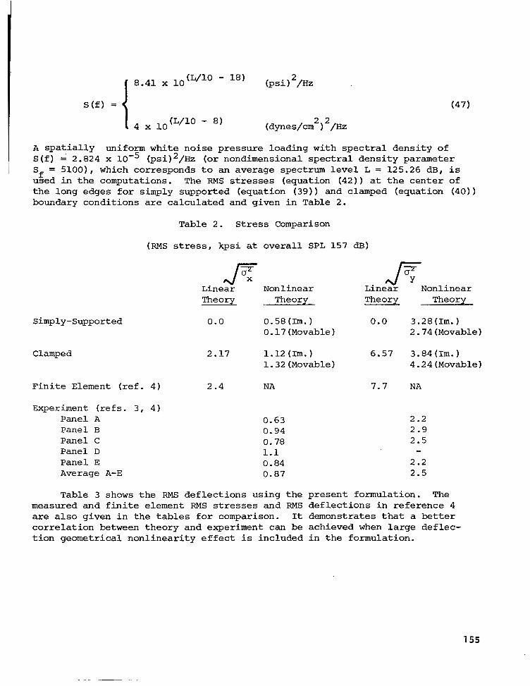
8.41 x 1 0 (L/10 - 18) (psi) 2 /Hz

S ( f ) =

(L/10 - 8 ) 2 2 4 x 1 0 (dynes/cm 1 /Hz

(471

A s p a t i a l l y u n i f o r m w h i t e n o i s e p r e s s u r e l o a d i n g w i t h spectral d e n s i t y o f S ( f ) = 2.824 x (psiI2/Hz (or nond imens iona l spec t r a l dens i ty parameter Sf = 5100), which corresponds t o an average spec t rum leve l L = 125.26 dB, is used in the computa t ions . The RMS s t r e s s e s ( e q u a t i o n ( 4 2 ) ) a t t h e c e n t e r of the long edges for s imply supported (equat ion (39)) and c lamped (equat ion (40) ) boundary condi t ions are c a l c u l a t e d a n d g i v e n i n Table 2.

Table 2 . S t r e s s Comparison

(RMS stress, kps i a t o v e r a l l SPL 157 dB)

Simply-Supported

Clamped

JT Linear Nonlinear Linear Nonlinear Theory Theory Theory Theory

0.0 0.58 (Im. ) 0.0 3.28(Im.) 0.17 (Movable ) 2.74 (Movable)

2.17 1 .12 ( I m . ) 6.57 3.84 ( I m . ) 1.32 (Movable) 4.24 (Movable)

F i n i t e Element ( r e f . 4 ) 2 .4 NA 7.7 NA

Experiment (refs. 3, 4 ) Panel A Panel B Panel C Panel D Panel E Average A-E

0.63 0.94 0.78 1.1 0.84 0.87

2 .2 2 .9 2.5 - 2.2 2.5

Table 3 shows t h e RMS d e f l e c t i o n s u s i n g t h e p r e s e n t f o r m u l a t i o n . The measured and f i n i t e e l e m e n t RMS stresses and RMS d e f l e c t i o n s i n r e f e r e n c e 4 are a l s o g i v e n i n t h e t a b l e s f o r c o m p a r i s o n . It d e m o n s t r a t e s t h a t a better cor re la t ion be tween theory and exper iment can be ach ieved when large d e f l e c - t i o n g e o m e t r i c a l n o n l i n e a r i t y e f f e c t is i n c l u d e d i n t h e f o r m u l a t i o n .

155

Table 3 . Deflection Comparison

Simply Supported

Clamped

F in i t e E lemen t ( r e f . 4 )

Measured (refs. 3, 4 )

J- max

Linear Theory

8.0

2.7

3.1

Nonlinear Theory

1.8 (Immovable) 2.4 (Movable)

1 .4 (Immovable 1 1 .6 (Movable 1

NA

2.0

CONCLUDING REMARKS

An a n a l y t i c a l method f o r p r e d i c a t i n g r e s p o n s e of r e c t a n g u l a r n o n l i n e a r s t r u c t u r a l p a n e l s s u b j e c t e d t o b r o a d b a n d random a c o u s t i c e x c i t a t i o n i s presen ted . The formula t ion is based on the Karman-Hermann large def lect ion plate equa t ions , a s ingle-mode Galerk in approximat ion , the equiva len t linear- i z a t i o n method, and an i te ra t ive p rocedure . Both s imply suppor ted and c lamped suppor t cond i t ions w i th immovable or movable inplane edges are considered. Panel mean-square def lect ion, maximum mean-square stress, a n d e q u i v a l e n t l i n e a r frequency a t g i v e n e x c i t a t i o n p r e s s u r e spectral dens i ty can be de te rmined , and t h e y are presented in g raphica l form. These g raphs can be used as g u i d e s f o r pre l iminary des ign of a i rc raf t pane ls under h igh no ise envi ronment . Resul t s ob ta ined ag ree w e l l wi th the exper iment . It is s u g g e s t e d t h a t f u r t h e r r e s e a r c h b e c a r r i e d o u t w i t h special a t t e n t i o n t o employ m u l t i p l e modes i n t h e f o m u l a - t i o n f o r accurate determination of mean-square stresses, a n d a d d i t i o n a l tes t d a t a on s imple pane l s are needed for an adequate quant i ta t ive compar ison .

REFERENCES

1. Rudder, F. F. , Jr. and Plumblee , H. E. , Jr. , "Sonic Fatigue Design Guide f o r M i l i t a r y A i r c r a f t " , AFFDL-TR-74-112, W-PAFB, OH, May 1975.

2 . F i t c h , G. E. " e t a l , "Establishment of the Approach t o and Development of Interim Design Criteria fo r Son ic Fa t igue" , ASD-TDR-62-26, W-PAFB, OH, June 1962.

3. Van d e r Heyde, R. C. W. and Smith, D. L. , "Sonic Fa t igue Res is tance of Skin-St r inger Pane ls" , AFFDL-TM-75-149-FYAI W-PAFB, OH, A p r i l 1974.

156

4. Jacobs, L. D. and Lagerquis t , D. R., "Finite Element Analysis of Complex Panel t o Random Loads," AFFDL-TR-68-44, W-PAFB, OH, October 1968.

5. Jacobson, M. J., "Advanced Composite Joints : Design and Acoust ic Fat igue C h a r a c t e r i s t i c s , " AFFDL-TR-71-126, W-PAFB, OH, A p r i l 1972.

6. Jacobson, M. J., "Sonic Fatigue Design Data f o r Bonded Aluminum A i r c r a f t S t ruc tu res , " AFFDL-TR-77-45, W-PAFB, OH, June 1977.

7. Mei, C., "Large Amplitude Response of Complex S t r u c t u r e s Due t o High I n t e n s i t y Noise," AFFDL-TR-79-3028, W-PAFB, OH, April 1979.

8. Chu, H. N. and Herrmann, G. , "Influence of Large Amplitudes on Free Flex- ura l Vibra t ions o f Rec tangular Elastic Plates," J. of Applied Mechanics, V o l . 23, December 1956, pp. 532-540.

9. Caughey, T. K. , "Equivalent Linearization Techniques," JASA, V o l . 35, November 1963, pp. 1706-1711.

11. Spanos, P. T. D. and Iwan , W. D. , "On the Existence and Uniqueness of Solutions Generated by Equ iva len t L inea r i za t ion , " In t . J. of Non-Linear Mechanics, V o l . 13, 1978, pp. 71-78.

1 2 . Timoshenko, S. and Woinowsky-Krieger, S., Theory of Plates and She l l s , McGraw-Hill, 1959, pp. 415-428.

13. Lin, Y. K . , "Response of a Nonlinear F la t P a n e l t o P e r i o d i c a n d Randomly- Varying Loadings," J. A e r o . Sci., September 1962, pp. 1029-1033, p. 1066.

14. Yamaki, N . , "Influence of Large Amplitudes on Flexural Vibrat ions of Elastic Plates," 2. Angew. Math. Mech., Vol. 41, 1961, pp. 501-510.

15. Seide, P. , "Nonlinear Stresses and Deflect ions of Beams Subjected t o Random Time Dependent Uniform Pressure," ASME Paper No. 75-DET-23, 1975.

16. Seide, P., "Large Deflections of Prestressed Simply Supported Rectangular Plates under Uniform Pressure," Int . J. Non-Linear Mechanics, Vol. 13, 1978, pp. 145-156.

17. Van d e r Heyde, R. C. W. and Wolfe, N. D. , "Comparison of t he Son ic Fa t igue Charac t e r i s t i c s of Four Structural Designs," AFFDL-TR-76-66, W-PAFB, OH, September 1976.

157

sy

Figure 1. Geometry and coordinates.

/' IMMOVABLE EDGES MOVABLE EDGES "_

Figure 2 . Mean-square deflection versus spectral density parameter of excitation for simply supported panels, 5 = 0.02.

1 58

600 c N

400

- IMMOVABLE EOGES "_ MOVABLE EDGES

I I l I l l 0 5000 10000 15000 20000

Figure 3. Maximum mean-square stress versus spectral density parameter of excitation for simply supported panels, 5 = 0.02.

IMMOVABLE EOGES "_ MOVABLE EOGES

Figure 4. Effect of damping on mean-square deflection for a simply supported square panel.

1 59

........... , , . . . - I

IMMOVABLE EDGES "- MOVABLE EDGES

Figure 5. Effects of damping on maximum mean-square stress f o r a simply supported square panel.

7000 -

- 6000 - "-

5000 - x 4000 -

3000 -

IMMOVABLE EOGES MOVABLE EDGES

0 1 2 3 4 5 6

Figure 6. Frequency parameter versus mean-square def lec t ion for s imply suppor ted pane ls .

7 60

IMMOVABLE EDGES MOVABLE EDGES "-

I l l I l l l l l l l l l l l l l l l I 0 5000 10000 ' 15000 20000

Sf

Figure 7. Mean-square deflection versus spectral density parameter of excitation for clamped panels, 5 = 0.02 .

looor

IMMOVABLE EDGES "- MOVABLE EDGES

0 50UO 10000 15000 20000 Sf

Figure 8. Maximum mean-square stress versus spectral density parameter of excitation for clamped panels, 5 = 0.02.

161

3.5 r / 3.0

2.5

.2.0 ’

LINEAR -

Figure 9. Effects of damping on mean-square deflection for a clamped square panel.

lMMOVABLE EOGES MOVABLE EOGES

/

I 0 0.5 1.0 1 . 5 2.0 2.5 3.0 3.5

Figure lo. Frequency parameter versus mean-square deflection for clamped panels.

162

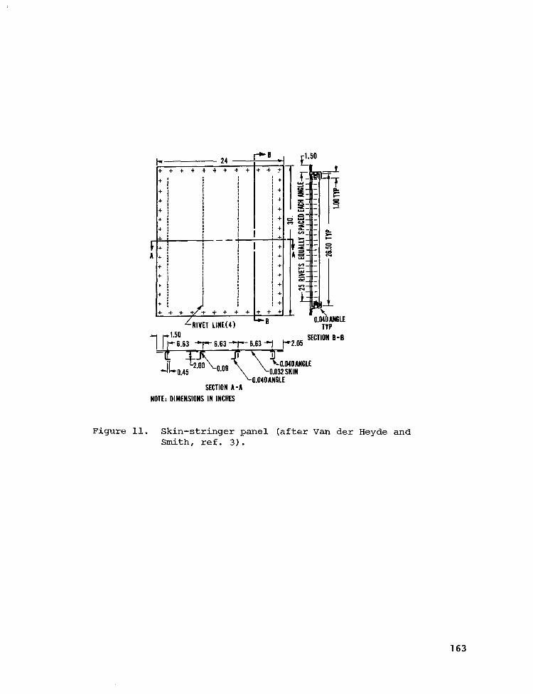
L0.040AN6LE SECTION A - A

NOTE: DIMENSIONS IN INCHES

Figure 11. S k i n - s t r i n g e r p a n e l ( a f t e r Van der Heyde and Smith, ref. 3 ) .

163

POST-BUCKLING BEHAVIOR OF A BEAM-COLUMN

ON A NONLINEAR ELASTIC FOUNDATION WITH A GAP'

Edward N. Kuznetsov Battelle Columbus Laboratories

Thomas G. Johns Battelle Houston Operations

SUMMARY

The subject of this paper is the structural behavior of an elastic beam- column placed with a gap between two nonlinearly elastic layers each resting on a rigid foundation. The beam-column is laterally supported at both ends and subjected to a uniform transverse load and axial compression. Its slenderness is such that the axial compressive force exceeds the amount that would be necessary to buckle it as a simply supported column. The elastic layers are represented by an elastic foundation with a strongly nonlinear specific reaction taken as a rapidly increasing function of the layer compression. The analytical model developed simulates the entire pattern of the deflection and stress state including layer and end support reactions, under gradually increasing axial force.

INTRODUCTION

There are many cases when a primary buckling mode occurring at the onset of buckling cannot develop freely (References 1-2) because of changing constraint or support conditions. Such is, in particular, the case of a column with lateral supports arranged with gaps, etc. In this case, the post-buckling deflection is constrained laterally and the axial force can be increased by far in excess of its first critical value. As a result, the structural behavior is characterized by a sequence of alternating gradual changes in the deformed configuration and rather abrupt jumps fromone equilibrium configuration to another. A similar behavior pattern was observed (Reference 3 ) for a compressed plate.

The subject of this paper is an elastic beam-column placed with a gap between two nonlinearly elastic layers each resting on a rigid foundation (Figure 1). The beam-column is laterally supported at both ends and subjected

This study was sponsored by the American Gas Association Pipeline Research Committee .

1 65

to a uniform transverse load and axial compression. The elastic layers have a strongly nonlinear specific reaction taken as a rapidly increasing function of the layer compression. The problem consists in the analytical evaluation of the stress state and deflection under gradually increasing axial compression.

The deflection of the beam-column in consideration is small enough to justify the use of.the conventional linearized expression for the curvature. However, there are two other sources of nonlinearity (nonlinearly elastic layers and the presence of a gap) which were fully accounted for. Note, that the presence of a transverse load makes the problem nonhomogeneous so that it is not a bifurcation problem.

ANALYTICAL FORMlTLATION AND SOLUTION METHOD

Under the above assumptions, vertical equilibrium of the beam-column requires that

F(Y) EIY(X)I~ + PY(X)II + Q(Y(~)) - G = 0 (1)

Here Y is the elastic deflection of the beam-columny E1 is its flexural rigidity, is the axial compression force, Q(Y) is the foundation reaction per unit length as a function of Y, G is the distributed transverse load (assumed uniform and constant), x' is the column longitudinal axis and prime denotes differentiation with respect to x.

The elastic foundation reaction is taken in the following form:

where k and n are given constants and c is the gap size. Thus, the foundation reaction is proportional to a power of the beam-column penetration into the elastic layer.

The self-correcting finite increment method (Reference 4 ) will now be applied for solving Equation (1). To this end the compression force P is given an infinitesimal increment p which results in some infinitesimal variation y(x) of deflection Y (x) :

F(Y+y) F E1 (Y+y) + (P+p) (Yt-y) 'I + Q (Y+y) - G = 0 . IV (3)

Specializing Q(Y) in accordance with Equation (2) yields

F (Y) + EIy IV + Py" + pY1' +{ 0 kn (Y-c) n-ly

- G = 0 .

1 66

The operation performed is known as Frechet differentiation. It resulted in a linearized equation in unknown variation y(x) and is rigorous for infinitesimal increments only. The equation is extrapolated to small but finite increments which permits itsuse in a step-by-step solution procedure. A solution obtained at each step is an approximate one. Therefore, employing it as a starting point for the next step introduces some error in addition to that resulting from the next step itself. This is partially offset by a correction which consists in retaining the first term in Equation ( 4 ) . For an exact Y(x), this term, according to Equation (1) would be an identical zero. Since in reality the solution obtained after the m-th step,

Y"(X) = Ym-l(x) + ym(x) , is approximate, it does not turn F(Y) into zero. Retaining this term in Equation ( 4 ) compensates for the error of a current step solution thus preventing both systematic and occasional errors from passing to the next step and accumulation.

The solution of linearized Equation ( 4 ) is sought in the form of a linear combination of several approximating functions satisfying the boundary conditions of the problem:

where R is the beam half-length (Figure 2). As is readily seen, only symmetric configurations of the beam are taken into consideration. This was done because the particular case of interest is characterized by a relatively big transverse load, which precludes the antisymmetric configurations from occurrence at the early stages of post-buckling deformation. (The uniform transverse load would perform zero mechanical work over antisymmetric displacements).

The Galerkin method is now applied. It requires substituting the above y(x) into Equation ( 4 ) , multiplying it by one of the approximating functions and integrating the product over the beam length. This results in a system of N linear algebraic equations in unknown parameters y with coefficients i

R

and free terms

a = (DiEI-P)Di t + sS(x) sin 2R dx 2 (2i-1)rx ii 0

R aij = J S(x)sin (2i-1)nx sin (2j-1)rx dx

0 2R 2R

R

a = - D ~ Y ~ ~ + JF(~) sin (2i-1) rx 2R io 0 ( 8 )

1 67

where n

S(x) = kn[Y (x)-cln-'

N'

Obviously, making the

D.Y.sin (2i-l)~x 1 1 2R + Q [Y(x)l-G

(10)

axial force increments smaller improves the accuracy of the solution, but increases the number of solution steps. A reasonable compromise was achieved by arranging intermediate iterations in which Equation ( 4 ) was solved without incrementing the axial force (i.e., setting p = 0). In these iterations, the pattern of the beam interaction with the elastic layers is refined for the fixed magnitude of the axial force. Only after some assigned level of accuracy is reached, the axial force is given its next increment.

The specificity of the problem in consideration is that more than one equilibrium configuration may correspond to a given axial force. To determine whether other equilibrium configurations exist in the vicinity of the original one, the following approach is employed. Upon achieving the convergence of the internal iterations for a fixed value of the axial force, the system is perturbed by giving the deflection some random distortion and internal iterations are performed once again. This may result in overcoming the energy barriers separating the possible equilibrium configurations and increases the likelihood of solution convergence to the most stable configuration.

The perturbation is physically meaningful: it reflects imperfections in material properties, system geometry, load application and many other factors not accounted for explicitly. The magnitude of the distortion presumably correlates with the mentioned imperfections.

A computer program implementing the above features was written and applied to the analysis of a precompressed cryogenic pipeline.

NUMERICAL RESULTS AND DISCUSSION

The concept of preshortening a cryogenic pipeline by compression is intended to reduce or eliminate the need for thermal expansion/contraction devices. The concept involves the compression of one pipe (inner, conveying pipe) within another (casing pipe). The pipes are separated by thermal insulation and an air gap (clearance) exists between the insulation and the inner or the outer pipe. The magnitude of the compressive force is limited by the amount that can be tolerated in the inner pipe wichout its local inelastic buckling as a cylindrical shell (Reference 5) . Under this force,

1 68

tigated to determine the effect of design variables such as the gap size, pipe length, insulation elastic properties, etc., upon the maximum stresses, lateral reactions, and amount of absorbed compressed length.

The following, rather typical data were used in one of the numerical examples :

0 pipe length - 100 m (328 ft) 0 pipe outer diameter - 46.7 cm (18 inches) 0 wall thickness - 0.9525 cm (3/8 inch) 0 clearance - 2.54 cm (1 inch) 0 permissible stress - 320 MF'a (46 ksi).

Figure 3 shows the evolution of the elastic deflection of the pipe as the compression force grows. Diagram 3a is the sagged configuration of the pipe resting on the elastic layer almost uniformly compressed. As the axial force is increased, the pipe bends and develops progressively increasing waviness (3b and c) till the end segment ''snaps through" (3d). At this moment the pipe assumes another equilibrium configuration which continues its evolution in further loading (3e).

The results of numerical experiments confirmed the role of systematic perturbations applied during the analysis in order to obtain equilibrium states with lower total energy. In all cases the self-correcting finite increment method provided a rapid convergence of the computation process.

From the viewpoint of the precompression concept it was important to establish the role of the gap between the pipe and insulation. Conceivably, a wider gap could even be an advantage since it would provide more room with which to absorb the ''excess" pipe length. A parametric study showed, however, an adverse effect of the gap on the relative compression of the pipe: the wider the gap, the greater the portion of the material strength spent on bending stress. Interestingly, the maximum stress (composed of the axial and bending stresses) does not grow monotonically with the compression force.

The performed study also revealed the role of the pipe length. A s shown in Figure 4 , the amount of compression that can be absorbed without exceeding the permissible stress increases for shorter lengths of pipe. The limiting case is the pipe length at whichoverallbuckling does not occur at all.

1 69

REFERENCES

1. Thompson, J.M.T. and Hunt, G. W., "A General Theory of Elastic Stability," Wiley, London, 1973.

2. Budiansky, B., "Theory of Buckling and Post-Buckling Behavior of Elastic Structures," Advances Appl. Mech., Vol. 14, Academic Press, 1974.

3. Nakamura, T. and Uctani, K . , Int. J. Mech. Sci., Vol. 21, No. 5, 1979.

4. Mescall, J., "Numerical Solutions of Nonlinear Equations for Shells of Revolution," AIAA Journal, Vol. 4, No. 11, 1966.

5. Volmir, A. S., "Stability of Elastic Systems," Moscow, 1963. (WPAFB Translation AD 628508, 1966).

1 70

P-)-

Figure 1.- Beam-column between two layers of elastic foundation with gap.

Figure 2.- Buckled column segment with partial contact with foundation.

171

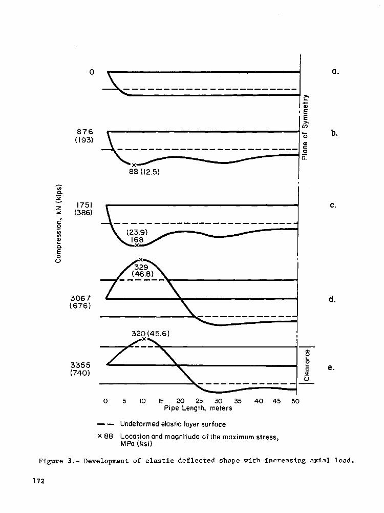
0

876 (193)

I751 (386)

3067 ( 6 7 6 )

3355 (740)

Figure

. .

"""""""""""_ t E

' E I!

\ 16 W E 0 """""""""""" - n

"""

a.

b.

C.

d.

320 (45.6)

W V E

0 e. - W 0

0 5 IO 15 20 25 30 35 40 45 50 Pipe Length, meters

- - Undeformed elastic layer surface

X 88 Location and magnitude of the maximum stress, MPa (ksi)

3.- Development of elastic deflected shape with increasing axial load.

172

I .75 1 I I I

u = 320 MPa (46 ksi) c = 2.54 cm ( I inch)

m 0

2 ti

1.50 - c -

.-

c 0 v) u)

.-

E 1.25 - E

-

0 0

I .oo I 1 I I 0

~-

25 (82) 5 0 (164) 75 (246) 100 (328) Pipe Length, m(f t )

Figure 4 . - Amount of compression that can be absorbed without exceeding t h e a l l o w a b l e stress v e r s u s p i p e l e n g t h .

173

STRAIGHTENING OF A WAVY STRIP - AN ELASTIC-PLASTIC

CONTACT PROBLEM INCLUDING SNAP-THROUGH

D i e t e r F. Fischer and Franz G. Rammerstorfer VOEST-ALPINE AG, FAT, L inz , Aus t r i a

SUMMARY

Thi s paper d e a l s w i t h c a l c u l a t i n g t h e n o n - l i n e a r b e h a v i o u r o f a wave-like deformed metal strip d u r i n g t h e l e v e l l i n g p r o c e s s . E l a s t i c - p l a s t i c material behaviour as we l l as n o n l i n e a r i t i e s d u e t o l a r g e d e f o r m a t i o n s a r e c o n s i d e r e d . The cons idered problem leads to a combined s t a b i l i t y and contact problem. I t is shown t h a t , d e s p i t e of t h e i n i t i a l l y c o n c e n t r a t e d l o a d i n g , n e g l e c t i n g t h e change of loading condi t ions due to a l te red contac t domains may l e a d t o a s i g n i f i c a n t e r r o r i n t h e e v a l u a t i o n o f t h e n o n l i n e a r b e h a v i o u r a n d p a r t i c u l a r l y t o a n u n d e r e s t i m a t i o n o f t h e s t a b i l i t y l i m i t l oad . The s t a b i l i t y i s examined by cons ide r ing t he l oad de f l ec t ion pa th and t he behav iour of a load-dependent c u r r e n t s t i f f n e s s p a r a m e t e r i n c o m b i n a t i o n w i t h t h e d e t e r m i n a n t o f t h e c u r r e n t s t i f f n e s s m a t r i x .

INTRODUCTION

The s t a b i l i t y o f n o n l i n e a r s t r u c t u r e s i s the goa l o f many r e c e n t p a p e r s . Espec ia l ly t he snap - th rough behav iour o f i n i t i a l ly cu rved s l ende r ba r s has been a n a l y t i c a l l y a s w e l l a s n u m e r i c a l l y c o n s i d e r e d ( e . g . r e f . 1 ,2 ) . B u t i n v e s t i g a t i o n s i n which the inf luence of contact between the loading and the l o a d e d s t r u c t u r e s is c o n s i d e r e d a r e r a t h e r r a r e . Such a combined c o n t a c t and s t a b i l i t y p r o b l e m w i l l b e t r e a t e d i n t h i s p a p e r . I n o r d e r t o show how t h e load ing cond i t ions i n f luence t he non l inea r behav iour and t he s t ab i l i t y l i m i t i n p a r t i c u l a r , l e t us draw our a t ten t ion to the fo l lowing s imple example .

F igure 1 shows a sha l low c i r cu la r a r ch wh ich is l o a d e d o n c e d i r e c t l y by a concen t r a t ed l oad and i n a second case by a r i g i d h o r i z o n t a l p l a n e plate moved towards the a rch . The la t ter is t r e a t e d as a contac t p roblem. In bo th cases , symmet ry w i th r e spec t t o t he ve r t i ca l ax i s is assumed f o r s i m p l i c i t y .

Applying the algorithm which is desc r ibed la ter w e g e t r e s u l t s shown i n f i g u r e 2. I n f i g u r e 2 the load d i sp lacement pa th , P ( w ) , the dependence of the no rma l i zed de t e rminan t o f t he cu r ren t s t i f fnes s matrix, d e t & ( P ) , a n d o f t h e c u r r e n t s t i f f n e s s p a r a m e t e r ( r e f . 3 , 4 ) , CS(P) , on the appl ied load , P , is d e s c r i b e d . I n b o t h c a s e s , d i s t i n c t s n a p - t h r o u g h b e h a v i o u r c a n b e o b s e r v e d b y cons ide r ing t he f i na l t angen t o f t he de t&(P) cu rve wh ich c ros ses t he P -ax i s p e r p e n d i c u l a r l y ( r e f . 5 ) . A l s o t h e v a n i s h i n g c u r r e n t s t i f f n e s s p a r a m e t e r , CS, indicates snap-through. However i n t h e case b (load a p p l i c a t i o n by a r i g i d p l a t e ) a s i g n i f i c a n t l y h i g h e r s t a b i l i t y l i m i t t h a n i n case a w a s found. Thus,

175

it is important to recognize the altering loading conditions even if the load is applied-at a single point in the initial state (i.e. at a very low load level). The problem being dealt with in the following chapters is a typical stability and contact problem.

DESCRIPTION OF THE WAVED STRIP PROBLEM

The behaviour of an infinite strip with periodic wave-like initial out- of-plane deformations is investigated during a straightening process. Periodic out-of-plane deformations at the boundaries (fig. 3 ) or in the middle domain of the strip sometimes appear in metal sheets as a consequence of the rolling process. The straightening is based on plastic deformations caused by moving the strip through a leveller in which it is bent by rollers in a repeated manner. In some cases, a snap-through of the waves can be observed which renders an unsuccessful result of the levelling process. In order to find p r o p conditions for avoiding snap-through, a procedure for calculating the nonlinear elastic-plastic stability problem was developed. The deformations during levelling are caused by rather stiff rollers. A contact problem has to be solved simultaneously with the stability problem in order to account for the stiffening effect due to expanded contact.

To approach the real behaviour of the waved strip during the levelling process by mathematical investigation, the complicated transient problem is simplified to a static consideration: The nonlinear behaviour of the shaded area of the strip in figure 3 under a downward moving rigid roller is calculated with the aid of the finite element method.

THE MATHEMATICAL MODEL

The following data were taken from an example in which instabilities in the practical levelling process were observed: B = 3500 mm, L = 1000 mm, S = 20 mm, t = 10 mm. The material is assumed to be elastic-plastic with linear strain hardening. The following material properties correspond to experimentally derived values at a temperature of 600 OC (the strip temperature during the levelling process): E = 180000 N/mm2 (Youngs' modulus), v = 0.3 (Poisson's ratio) , cry = 130 N/mm2 (initial yield stress) , ET = 5000 N / m 2 (strain hardening modulus). The shaded area in figure 3 under consideration represents a doubly curved shallow shell which is modeled using ADINA shell elements (ref. 6). These elements allow for nonlinear material behaviour as well as geometric nonlinearities using the total Lagrangian formulation. Figure 4 shows the finite element model.

The midsurface of the shell is approximated by

z (x,y) = S ~2 sin 4Y2 (L-2x1 IT 2L

As shown in reference 7 the contact conditions can be verified with the aid of contact elements. These contact elements are simple truss elements

1 76

which have a certain nonlinear elastic material behaviour (figure 5).

The contact elements give only contributions to the global current stiffness matrix if the shell nodes to which they are attached belong to the contact area. They allow only transmission of compression forces corresponding to the contact pressure. Before a shell node becomes a contact point, the gap between the rigid roller and the shell surface must be closed. This is accounted for in the location-dependent activating strain, ~ ~ ~ ~ ( y ) :

E s-2 (x=O,y)

gap = - S+h-z(x=O,y) The values of the tangent moduli, El, E2, the stresses, al" and ~72~:~ the

fictitious length, h, and the cross section area, A, of the contact elements must be properly chosen. This means that the contact elements should be stiff enough to prevent the roller from penetrating in the shell and, that the properties must not lead to a numerical instability of the incremental- iterative algorithms described below. The following values appear in the presented analysis: E1 = 1000 N/mm2, 02"= -20 N / m 2 , h = 80 mm, A = l o 0 0 mm . These values render a well- conditioned system of equations. If one would like to regard the local compressibility of the roller, a certain choice of the a-E-behaviour of the contact elements would make it possible. Furthermore, bending deformations of the roller could be considered, if beam elements would represent the axis of the roller instead of the rigid line (figure 4). Both effects, local compressibility and bending of the roller, are negligible in the investigated example.

E$ = 7500 N/mm2, ~ 1 " = -5 N/m2,

In order to represent the periodicity of the structure, the boundary conditions of the finite element model are introduced as shown in figure 4. The waved strip will elongate globally due to the levelling process. For the x-displacement at the boundary x = L/2 the following restriction is valid: ux(x=L/2,y) = ux(x=L/2,y=0).

DESCRIPTION OF THE ALGORITHMS

The analysis is performed in an incremental-iterative manner, using the tangent stiffness matrix concept and the BFGS iteration procedure as described elsewhere, e.g. in references 8,9. Let us concentrate our attention to the stability algorithms. Algorithms which treat nonlinear stability problems as a sequence of eigenvalue problems are described in recent papers (e.g. ref. 10 - 12). Let us now use the normalized determinant of the current tangent stiffness matrix, detnE, and the current stiffness parameter, CS, recently introduced by Bergan (ref. 3,4) as indicators for the stability behaviour of the structure during the lowering of the rigid roller. It is a well-known fact that at the stability limit, X-Xcrit (X ... load amplifier, Xcrit ... critical load amplifier), the determinant of the tangent stiffness matrix vanishes:

lim det &(X) = 0. A-Xcrit

T h i s c r i t e r i o n h o l d s f o r b o t h b u c k l i n g as w e l l as snap-through because it is based on t h e e x i s t e n c e of a n o n t r i v a l s o l u t i o n du o f t h e e q u a t i o n -

* - K ( X c r i t ) - f& = 0,

v a l i d a t t h e b i f u r c a t i o n p o i n t a n d a t the snap-through point .

One can d i s t inguish be tween buckl ing and snap- through by cons ider ing t h e d e t e r m i n a n t a p p r o a c h e s z e r o ( r e f . 5 , l O ) : I n t h e b u c k l i n g c a s e

h o l d s . I f t h e d e t e r m i n a n t b e h a v e s a c c o r d i n g t o

1 i m

A-Acrit

- = --a, a de t K

ax

how

( 5 )

snap-through is i n d i c a t e d .

The Gauss e l iminat ion procedure which is implemented i n ADINA ( r e f . 6 ) i s used i n c o m b i n a t i o n w i t h t h e L D g f r a c t o r i z a t i o n ( r e f . 1 3 ) t o s o l v e t h e f i n i t e e lement equa t ion sys tem dur ing the incrementa l - i te ra t ive ana lys i s . Thus , it is a l m o s t n o e f f o r t t o c a l c u l a t e t h e d e t e r m i n a n t of t h e nxn s t i f f n e s s m a t r i x u s i n g the f o l l o w i n g r e l a t i o n s :

K = L D L , T - ”_

- L is a l o w e r u n i t t r i a n g u l a r m a t r i x a n d is a diagonal matr ix . Hence,

d e t = d e t 2 = IT D . n i=l ii ( 8 )

T h i s d e t K is normalized so t h a t d e t , K(A=O) = 1. A t e ach l oad l eve l a t which a f u r t h e r c o n t a c t e l e m e n t is a c t i v a t e d , t h e c u r r e n t g l o b a l s t i f f n e s s m a t r i x increases suddenly due t o the added con t r ibu t ion o f t he ac t iva t ed con tac t e l e m e n t . I n o r d e r t o a v o i d d i s c o n t i n u i t i e s i n t h e d e t & ( A ) c u r v e t h e c u r r e n t de tn va lues are smoothened by a fu r the r no rma l i z ing p rocedure wh ich l eve l s t he d e t , v a l u e j u s t af ter a jump t o t h a t which appeared immediately before it. I t migh t be p rope r t o de l e t e a l l c o n t r i b u t i o n s r e l a t e d t o t h e c o n t a c t e l e m e n t s f r o m t h e c u r r e n t s t i f f n e s s m a t r i x i f d e t n K ( A ) is c a l c u l a t e d . T h i s would r e p r e s e n t t h e d e t e r m i n a n t b e h a v i o u r o f t h e s h e l l i t s e l f a n d t h e c o n t a c t would on ly con t r ibu te t o t he l oad vec to r on t he r i gh t -hand s ide o f t he i nc remen ta l f i n i t e e l e m e n t e q u a t i o n s .

The c u r r e n t s t i f f n e s s p a r a m e t e r , CS , has the fol lowing meaning (i i

denotes the increment number) : It r e p r e s e n t s t h e c u r r e n t s t i f f n e s s of t h e s t r u c t u r e as be ing a r e l a t ion be tween a load increment and the corresponding displacement increment. Assuming proportional loading one can express

i i - R = X S e f . (9)

i

r e f e r e n c e l o a d v e c t o r . R e l a t i n g t h e c u r r e n t s t i f f n e s s t o t h e i n i t i a l s t i f f n e s s R d e n o t e s t h e e x t e r n a l l o a d v e c t o r a t l o a d l e v e l A , Gef is t h e c o n s t a n t

i

178

( W i t h (< 1) CS can be de f ined as i

i i-1 i i-1 i cs = ( x- W I I 11.- UII 1 1 x/II u II (10)

us ing the Eucl idean norm o f t he i nc remen ta l d i sp l acemen t vec to r t o scale t h e r e l a t i o n s .

The combination of the d e t e r m i n a n t a n a l y s i s a n d t h e c u r r e n t s t i f f n e s s parameter c a l c u l a t i o n o f f e r s a good t o o l t o p r e d i c t t h e s t a b i l i t y l i m i t , X c r i t l as w e l l as t h e i n s t a b i l i t y mechanism ( i . e . buck l ing o r snap - th rough) as shown i n r e f e r e n c e 14.

DISCUSSION OF THE FESULTS

Figure 6 shows t h e l o a d d i s p l a c e m e n t p a t h o f t h e i n i t i a l c o n t a c t p o i n t (node A i n f i g u r e 4 ) , t he no rma l i zed de t e rminan t o f t he s t i f fnes s ma t r ix , d e t n ( ( h ) , a n d t h e c u r r e n t s t i f f n e s s p a r a m e t e r , C S ( h ) . The results o f t he a n a l y s i s o f t h e same s h e l l l o a d e d by a concen t r a t ed l oad i n A are a l s o p r e s e n t e d i n f i g u r e 6 as a comparison. The fo l lowing f ac t s can be obse rved : In both cases a s t a b i l i t y l i m i t is reached and snap-through of the wave takes p lace . The s h e l l l o a d e d b y t h e r o l l e r b e h a v e s s i g n i f i c a n t l y stiffer than t he po in t - loaded she l l . Th i s is caused by t he a l t e r ing l oad ing cond i t ions due t o t h e i n c r e a s i n g c o n t a c t domain as expla ined above . In the concent ra ted load approach, a ho r i zon ta l t angen t o f t he l oad d i sp l acemen t pa th is reached before c o n s i d e r a b l e p l a s t i f i c a t i o n t a k e s p l a c e . I n t h e c o n t a c t s o l u t i o n , p l a s t i c domains appear i n t h e v i c i n i t y o f t h e c o n t a c t a r e a l o n g b e f o r e a s i g n i f i c a n t s t i f f n e s s loss ( i .e . a r ap id dec rease o f C S ) can be observed.

I n f i g u r e 7 the deformed s ta te of the she l l immedia te ly before snap- through is shown. One can see t h a t t h e c o n t a c t domain between r o l l e r a n d s t r i p is considerable . Furthermore, it i s i n t e r e s t i n g t o n o t i c e t h a t t h e i n i t i a l c o n t a c t p o i n t A belongs no longer t o t h e c o n t a c t a r e a .

CONCLUSION

From these cons idera t ions one can conclude tha t neglec t ing the change of loading condi t ions due to deformation dependent contact condi t ions may l e a d t o a n u n n e g l i g i b l e e r r o r e v e n i f i n i t i a l l y c o n c e n t r a t e d l o a d c o n d i t i o n s are j u s t i f i e d .

179

REFERENCES

1. Pisanti, A.: Geometrically Nonlinear Behaviour of Initially Curved Plane Slender Bars and Frames. Inenieur-Archiv, Vol. 46, pp. 235 - 244, 1977.

2. Noor, A.K., Greene, W.H. and Hartley, S.J . : Nonlinear Finite Element Analysis of Curved Beams. Computer Methods Appl. Mech. Eng., V o l . 12, pp. 289 - 307, 1977.

3 . Bergan, P.G., Horrigmoe, G., Krakeland, B. and Sbreide, T.H.: Solution 0

Techniques for Non-Linear Finite Element Problems. Int. J. Numer. Methods Eng., V o l . 12, pp. 1677 - 1696, 1978.

4. Bergan, P.G.: Solution Algorithms for Nonlinear Structural Problems. Proc. Int. Conf. Eng. Appl. FEM, Hbvik, Norway, 1979.

5. Gallagher, R.H. and Mau, S.: A Method of Limit Point Calculation in Finite Element Structural Analysis, NASA CR-2115, 1972.

6. Bathe, K.-J.: ADINA, A Finite Element Program for Automatic Dynamic Incremental Nonlinear Analysis, M.I.T. Report 82448-1, Acoustics and Vibration Laboratory, Mechanical Engineering Department, Mass. Inst. Techn., 1975 (Rev. 1978).

7. Rammerstorfer, F.G., Fischer, D. and Zitz, A.: Rock Bursting - A Nonlinear Dynamic Contact Problem, Num. Methods in Geomechanics, W. Wittke, A.A. Balkema, Rotterdam, 1979.

8. Bathe, K.-J., Bolourchi, S., Ramaswamy, S. and Snyder, M.D.: Some Computational Capabilities for Nonlinear Finite Element Analysis. Nucl. Eng. Design, Vol. 46, pp. 429 - 455, 1978.

9. Matthies, H. and Strang, G.: The Solution of Nonlinear Finite Element Equations, Int. J. Numer. Methods Eng., V o l . 14, pp. 1613 - 1626, 1979.

lO.Ramm, E.: Geometrisch nichtlineare Elastostatik und finite Elemente, Habilitationsschrift, Univ. Stuttgart, 1975.

11.Brende1, B.: Geometrisch nichtlineare Elastostabilitat, Bericht Nr. 79-1, Inst. f. Baustatik d. Univ. Stuttgart, 1979.

12.Brende1, B., Ramm, E., Fischer, D. and Rammerstorfer, F.G.: Linear and Nonlinear Stability Analysis of Thin Cylindrical Shells Under Wind Loads. To be published in J. Struct. Mech., Vol. 9, 1981.

180

13. Bathe, K.-J. and Wilson, E.L.: Numerical Methods in Finite Element Analysis, Prentice-Hall, Inc., Englewood Cliffs, New Jersey, 1976.

14. Rammerstorfer, F.G. and Fischer, D.F.: Nonlinear Elastic-Plastic Stability and Contact Problems Concerning the Straightening of a Wave-Like Deformed Strip Plate. Proc. 1st Int. Conf. Num. Methods for Non-Linear Problems, Swansea, Pineridge Press, 1980.

1 81

d

2 000 -*

a 7

b EJ = 2.5x108Nmm2 EA= 3.0 x IO7 N

Figure 1.- The circular arch loaded by concentrated load directly (a) or via rigid plate (b) .

LOAD P

1.0

. 0

. 6

. 4

. 2

. o

I I CONTACT, CASE

‘x I \. C!J r-- -\ />

-\\

.2 .4 .6 .8 1,o 1.2 MIDPOINT DEFLECTION w 10’mm DETERMINANT det&P), CURR. STIFF PAR. CS

Figure 2.- Load displacement behaviour, normalized determinant of the current stiffness matrix and current sti€fness parameter for the two different loading conditions.

1 82

tl

S

X

1 83

Figure 5.- Schematic sketch of the contact element material behaviour.

.6

.5

LOAD -4 AMPL.

a .3

.2

.I

.o

7".

// -\ \ \ \ \

det& '\, \ \ \ \ \, \\ I.

I I I . 5 10 15 20

DISPLACEMENT u, mm

.o 2 4 6 .8 1.0 de t; &I), CS ( i t )

I I I I I I

Figure 6.- Results of the analysis of the wavy s t r ip p la te ob ta ined by (a) solving the contact problem and (b) concentrated load approach.

184

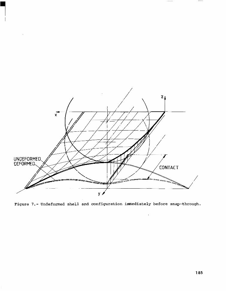
'1

,/

Figure 7.- Undeformed shell and configuration immediately before snap-through.

185

A PROPOSED GENERALIZED CONSTITUTIVE EQUATION FOR NONLINEAR

PARA-ISOTROPIC MATERIALS*

K.K. Hu, S.E. Swartz and C.J. Huang Department of Civil Engineering

Kansas State University Manhattan, Kansas

INTRODUCTION

With the advent of finite element models of varying complexity the focus of solutions to problems in solid mechanics has shifted very strongly into the direction of more accurate material description. This is especially true for materials for which strength characteristics vary widely with state of stress. In particular, concrete which is non-isotropic at any level of deformation and is also non-linear in terms of stress-strain relationships has been singled out for intensive study. This includes work on constitutive relations (refs. 1 to 51, and failure (refs, 3 , 4 , and 6 to 15).

Related developments in failure theories are those included in references 16 to 25.

This list is by no means exhaustive but formed a background basis which led to the model proposed in this paper. In particular, the developments in the areas of maximum deformation theory and the Von Mises-Hencky theory provided motivation for the concept used here (ref. 26).

FAILURE SURFACE

The proposed generalized constitutive equation is an extension of the work of Hu and Swartz (26) on the study of the failure of materials so that for any kind of material in any state. uf stress its mechanical behavior can be characterized by a single functional. According to the theory, a material failure initiates when the state of stress at a point is such that the following functional reaches a threshold value F :

0 O 1 O 2 a 3

aJ2 [ E ( o l ) - % q + E ( o j ) 11 (0 fC* ft)

F(Z) = c t C t + (l-a) 2 b f Of - ‘Of - Of 1 J1l t c

Ef (Of + J1> + pEf (of - J1) c t

(1)

* This research reported herein was supported in part by the National Science Foundation, Grant No. ENG 78-07829.

187

._ . .. . .. . . . "

In this equation

a = a material related scalar factor which is determined by experimental data.

J 1 = o + o + a

J2 = (al - a2)2 + (a2 - a3) + (a3 - Dl) . 1 2 3'

2 2

al, 02, o3 = the components of principal stresses, tensile stress ha? positive value. A vector of principal stresses is expressed by a.

a o = the absolute value of the ultimate stresses of the material under C

' uniaxial tension and compression, respectively.

E E = the absolute values of strain component in the direction of uniaxial C

' force when stress reaches the corresponding ultimate value.

E(o) = the secant modulus of elasticity of the material subjected to uniaxial stress (tension or compression as appropriate).

p = the Poisson's ratio of the material (related to stress level).

CONSTITUTIVE EQUATIONS

Non-linear response will take place when the increment of the functional is in an increasing manner and its value is beyond some threshold level (possibly zero). The material will be fractured at+ points where the state of stress reaches the surface of failure, i.e., F(o) = 1.

Between the initial state to fracture, the response is assumed to be characterized by Drucker's (17) theorem of orthogonality with the use of the functional proposed by the generalized failure theory, eqn. (1). That is, if the increment of principal strain components is decomposed into linear and non-linear increments,

{dE} = {dEe) + idsp}, (2)

the non-linear part is characterized by

where

G(;) = a scalar function of stresses,

{g(z)} = a unit vector of the gradient of the functional at the point of interest.

Note that G values (under uniaxial loading) can be determined by Some stress-

1 88

s t r a i n r e l a t i o n s h i p . In t h e g e n e r a l case, e s p e c i a l l y f o r t h o s e materials l i k e g l a s s o r c o n c r e t e , t h e G f u n c t i o n i n u n i a x i a l t e n s i o n d i f f e r s f r o m t h a t o f u n i - axial compression remarkably. Therefore a weighted average is proposed. Accord- i n g t o t h i s , t h e r e l a t i o n s h i p b e t w e e n t h e v e c t o r s a n d p r i n c i p a l strain increment a n d t h e p r i n c i p a l stress increment is proposed t o b e c h a r a c t e r i z e d by the fo l low- i n g g e n e r a l i z e d c o n s t i t u t i v e e q u a t i o n :

I n t h i s E = t h e m o d u l u s o f e l a s t i c i t y o f t h e material, LVF-I= t h e row vec tor o f

t h e g r a d i e n t of t h e f u n c t i o n a l a t t h e p o i n t o f i n t e r e s t , and t h e f u n c t i o n G ( Z ) is c a l c u l a t e d by

which is a weighted average accord ing to the va lues o f the cor responding pr inc i - p a l stress components. G . (a. ) depends on the value of t h e i - t h u n i a x i a l p r i n c i -

1 1 p a l stress and i s ca l cu la t ed acco rd ing t o

where g is t h e i - t h component of t h e unit vec tor {g} . i

I f U f C = U E = E and a = 1 is s e l e c t e d , t h e p r o p o s e d f a i l u r e t h e o r y C f Y f f

ag rees w i th t he Von Mises' t h e o r y a n d t h e g e n e r a l i z e d c o n s t i t u t i v e e q u a t i o n r e d u c e s t o t h e w e l l known P r a n d t l - R e u s s s t r e s s - s t r a i n r e l a t i o n ( r e f s . 4 , l l ) .

7 89

NUMERICAL EXAMPLE

Applying the proposed theory to plain concrete for the purpose of illustra- tion equ. (1) is. modified to read

F = - a J2 + (1-a) b1+P (a2+u3) 1 (af t+(sfc) t C (8)

afcaft - (af -af )J1 a c(l+v) + (af -paf )J1 c t f f

The implication used is an invariant modulus of elastic2ty and for concrete, so- called initial yield occurs at about .45 f’ .

C

Using test data for concrete (3) the level surfaces of the functional, the stress-strain curves of uniaxial tension and compression tests and the variations

of G [F(ai)] and G-[F(cri)] are shown in Figs. 1-3. The best value of a for

concrete is 0.46 which has been used in these curves.

+

Note in Fig. 1 the shape of the curve in the tension-compression zone follows very closely the shape of the experimental curve obtained by Kupfer, Hilsdorf and Rusch ( 3 ) . The stress-strain curves presented in Figs. 2 and 3 were obtained using testing equipment described in Ref. 27. Using these data, Equations 8 for

F and 7a and 7b for G+ and G- were evaluated numerically to obtain the curves displayed.

CONCLUSIONS

A proposed constitutive model for non-linear materials has been presented. The primary virtues of the model are its logical combination of distortion states, inherent simplicity and generality.

Results presented for the model applied to concrete show good agreement with published experimental data for failure. The model can be readily incorporated into existing computer codes provided sufficient experimental supportive data are available.

The proposed constitive equation is presently being utilized in the development of a finite element code for determination of unstable crack growth and stress intensity in concrete beams.

1 90

REFERENCES

1. Andenes, Einar, "Response of Mortar to Biaxial Compression, "Thesis presented to the Faculty of the Graduate School, University of Colorado, in partial fulfillment of the requirements for the degree of Masters of Science, Boulder, Colorado, 1974.

2. Chen, A. C. T., and Chen, W. F., "Constitutive Relations for Concrete." J. ASCE 101, EM 4, 1975, pp. 465-481.

3. Kupfer, Helmut; Hilsdorf, Hubert K., and Rusch, Hubert, "Behavior of Concrete Under Biaxial Stresses," J. American Concrete Inst., Vol. 66, NO. 8, Aug. 1969, pp. 656-666.

4. Palaniswamy, R., and Shah, S. P., "Fracture and Stress-Strain Relationship of Concrete Under Triaxial Compression," J. Struct. Div., ASCE 100, 1974, pp. 901-916.

5. William, K. J., and Warnke, E. P., Constitutive Model for the Triaxial Behaviour of Concrete, IABSE Proc., Seminar Concrete Structures Subjected to Triaxial Stress, LLL-1, ISMES, Bergamo, 1974.

6. Bresler, B., and Pister, K. S., "Failure of Plain Concrete Under Combined Stresses." Trans. ASCE, Vol. 122, 1957, pp. 1049-1059; Discussion, pp. 1060-1068.

7. Hannant, D. J., and Frederick, C. O., "Failure Criteria for Concrete in Com- pression." Mag. Concrete Res., Vol. 20, 1968, pp. 137-144.

8. Iyengar, K. T., Sundara, Raja, Chandrashekhara, K., and Krishnaswamy, K. T., Strength of Concrete Under Biaxial Compression," J. American Concrete 11

Inst., Vol. 62, No. 2, Feb. 1965, pp. 239-249.

9. McHenry, D., and Karni, J., "Strength of Concrete Under Combined Tensile and Compressive Stress," J. American Concrete Inst., Vol 54, No. 10, Apr. 1958, pp. 829-840.

10. Newman, K., and Newman, J. B., "Failure Theories and Design Criteria for Plain Concrete." Structure, Solid Mechanics and Engineering Design - Proceedings of the 1969 Civil Engineering Materials Conference, edited by M. Te'eni, Vol. 2, pp. 963-995.

11. Reimann, H., "Kritische Spannungszustande des Betons bei mehrachsiger," ruhender Kurzzeitbelastung, Deutscher AusschuB fur Stahlbeton 175, Berlin, 1965, pp. 35-63.

12. Saucier, K. L.., "Equipment and Test Procedure for Determining Multiaxial Tensil and Combined Tensil-Compressive Strength of Concrete," Technical Report C-74-1, U.S. Army Engineer Waterways Experiment Station, Vicksburg, Miss., March 1974.

191

13.

14.

15.

16.

17.

18.

19.

20.

21.

22.

23.

24.

25.

Vile, G. W. D., "Strength of Concrete Under Short-Time Static Biaxial Stress," International Converence on the Structure of Concrete, Paper F2, Sept . 1965. Wastlund, G., "New Evidence Regarding the Basic Strength Properties of Concrete," Betong, Stockholm, Vol. 3, 1937.

Weigler, H., and Becker, G., "Untersuchungen uber das Bruch-und Verformungs- verhalten von Beton bei Zweiachsiger Beanspruchung," Deutscher Ausschuss fur Stahlbeton, V. 157, Berling, 1963.

Argyris, J. H., Faust, G., and William, K. J.Limit Load Analysis of Thick-Walled Concrete Structures - A Finite Element Approach to Fracture, ISD-Report No. 166, University of Stuttgart (1975), also in Comp. Meth. Appl. Mech. Eng., Vol. 8, No. 2, 1976, pp. 215-243.

Drucker, D. C., "A More Fundamental Approach to Plastic Stress-Strain Solution", Proceedings, 1st U.S. National Congress Applied Mechanics, ASME, New York, 1951, pp. 487-491.

Cornet, I., and Grassi, R. C., "Study of Theories of Fracture Under Combined Stresses." J. Basic Eng., Vol. 83, No. 1, 1961, pp. 39-44.

Eisenstadt, M. M., MacMillan and Co.,

Grassi, R. C., and Biaxial Stresses. I'

Introduction to Machanical Properties of Materials, New York, 1971.

Cornet, I., "Fracture of Gray Cast Iron Tubes Under J. Appl. Mech., Vol. 16, No. 2 , 1949, pp. 178-182.

Mair, W. M., "Fracture Criteria for Cast Iron Under Biaxial Stress." N.E.L. report No. 261. National Engineering Laboratory, East Kilbride, Glasgow, 1966.

Murphy, Glenn, Advanced Mechanics of Materials, 1st Edition, p. 83, McGraw- Hill Book Co., New York, 1946.

Nadai, A., Theory of Flow and Fracture of Solids, 2nd ed., McGraw-Hill Book Co., New York, 1950.

Prandtl, L., "Spannungsverteilung in plastischen Koerpern," Proceedings of the 1st International Congress on Applied Mechanics, Delft, Technische Roekhandel on Druckerij, J. Waltman, Jr., 1925, pp. 43-54.

Reuss, E., "Beruecksichtigung der elastischen Formaenderungen in der Plastizitaetstheorie," Z. Angew. Math. Mech., 10, 1930, pp. 266-274.

192

26. Hu, K. K., and Swartz, Stuart E., "A Proposed Generalized Material Failure Theory," Proceedings of the 15th Midwestern Mechanics Conference, University of. Illinois at Chicago Circle, Chicago, Illinois, March 23-25, 1977, pp. 144-147.

27. Swartz, S. E., Hu, K. K., Huang, J., and Jones, G. L., "An Apparatus for Tensile Testing of Concrete", Experimental Mechanics, Vol. 19, No. 3, March 1979.

193

4

I /

Compressive Strain (UE)

1,500 2,000 2,500 3,000

0.2 0.4 0.6 0.8 1.0 ~

Figure 3.- Data of uniaxial compressive test of concrete.

194

(5 1

a f t

(5 2

f

- t

(5

3

Figure 1.- Yield and fracture surfaces of concrete.

195

I

Figure 2.- Data of uniaxial tensi le test of concrete.

196

FINITE ELEMENT ANALYSIS

OF HYPERELASTIC STRUCTURES

Farhad Tabaddor B .F .Goodrich Akron, Ohio

SUMMARY

Most h y p e r e l a s t i c materials are t r e a t e d as i n c o m p r e s s i b l e o r n e a r l y i n c o m p r e s s i b l e i n a n a l y t i c a l a p p r o a c h . The u s e of t h e p e n a l t y f u n c t i o n , t o a c c o u n t f o r n e a r i n c o m p r e s s i b i l i t y , i s d i scussed and compared t o t h a t of Lagrange mul t ip l ie r . A scheme t o u s e L a g r a n g e m u l t i p l i e r , w i t h o u t h a v i n g t.o treat i t as unknown, is a l s o p r e s e n t e d .

INTRODUCTION

I n t h e v a r i a t i o n a l f o r m u l a t i o n of t he f i n i t e e l emen t p rob lems of i ncompress ib l e med ia , t he i ncompress ib i l i t y cond i t ion i s in t roduced th rough t h e u s e o f L a g r a n g e m u l t i p l i e r ( 1 , 2 ) . T h i s m u l t i p l i e r is a n a d d i t i o n a l unknown sca l a r func t ion wh ich canbeacconmoda ted i n t he d i sc re t e mode l by d isp lacement shape func t ions o r by similar methods. The procedure re- s u l t s i n a n i n c r e a s e i n t h e number of unknowns.

The i n c o m p r e s s i b i l i t y c o n d i t i o n , a s i d e f rom be ing inconvenient in f i n i t e e l e m e n t a n a l y s i s , is an approx ima t ion fo r rubbe r l ike materials. Such approximation becomes increasingly less a c c u r a t e as the pe rcen tage o f ca rbon b l ack i nc reases i n t he rubbe r compound ( 3 ) . The exact enforcement o f i ncompress ib i l i t y i s t h e r e f o r e n o t a c t u a l l y r e q u i r e d .

I n t h i s work t h e n e a r i n c o m p r e s s i b i l i t y i s accounted for by use o f the p e n a l t y f u n c t i o n ( 4 ) i n t h e e x p r e s s i o n f o r t h e s t r a i n e n e r g y f u n c t i o n . The c o n s t i t u t i v e e q u a t i o n s are then ob ta ined in incrementa l form. This i s m o s t s u i t a b l e f o r a n o n l i n e a r f i n i t e e l e m e n t . The i n c o m p r e s s i b i l i t y i s shown t o b e c l o s e l y s a t i s f i e d f o r l a r g e p e n a l t y n u m b e r s . The

197

c o n s t i t u t i v e r e l a t i o n s w i t h p e n a l t y number are compared w i t h t h e exact s o l u t i o n f o r t h e i n c o m p r e s s i b l e case. It is shown t h a t f o r a given accuracy of t h e s o l u t i o n , t h e p e n a l t y number m u s t v a r y i n t h e c o u r s e o f f i n i t e e lement solut ion f rom element to e lement and f rom one increment to the next . Some n u m e r i c a l r e s u l t s are p r e s e n t e d t o i l l u s t r a t e t h e s e p o i n t s . A s imple scheme t o u s e v a r i a b l e p e n a l t y number i s a l s o p r o p o s e d . F i n a l l y the i nc remen ta l form of c o n s t i t u t i v e e q u a t i o n s f o r t h e case of incompressible material is de r ived f rom the s t r a in ene rgy func t ion w i th t he Lagrange m u l t i p l i e r . An a l t e r n a t i v e p r o c e d u r e is then proposed which does no t requi re t rea tment o f the Lagrange mul t ip l ie r as unknown.

BASIC EQUATION

The s t r a i n e n e r g y f u n c t i o n W f o r i s o t r o p i c h y p e r e l a s t i c materials has t he fo l lowing form:

\fiere 11, 1 2 , and h a r e the t h ree i nva r i an t s o f Green-Lagrange s t r a in t enso r and are r e l a t e d t o s t r a i n components, fo r t he ax i symmet r i c ca se , as fo l lows:

I 2 = 3 + 4 ( Y 1 1 + Y 2 2 + Y 3 3 + Y 1 1 Y 2 2 + Y 1 1 Y 3 3 + t t t t t t t

t t t Y 2 2 Y 3 3 - Y122)

t t t Y11 , Y22and Y 3 3 are t h e c u r r e n t v a l u e s of s t r a i n s . I n t h i s work, o n l y t h e

axisymmetric case i s considered. The discussion, however , can be extended Co the three-d imens iona l case w i t h o u t a n y d i f f i c u l t y . I n t h e a x i s y m m e t r i c r,ase, t h e s t r a i n i n v a r i a n t s are r e l a t e d t o c u r r e n t d i s p l a c e m e n t s by

1 98

x2 i s t h e axis of symmetry and ~ 1 x 2 i s t h e a x i s m e t r i c p l a n e . The c u r r e n t d i s p l a c e m e n t s p a r a l l e l t o x1 andxz axes are denoted bytul and U P

r e s p e c t i v e l y .

The second Piola-Kirchoff stress tensor components T a t c u r r e n t t i j

time, can be ob ta ined f rom the fo l lowing re la t ions

To o b t a i n t h e i n c r e m e n t a l form of c o n s t i t u t i v e e q u a t i o n s we d e f i n e

- t + A t t Yi j - Yij - i j i , j = 1,2,3

199

where T and Y..are inc remen ta l stress and s t r a in componen t s r e spec t ive ly . The i n c r e m e n t a l s t r e s s - s t r a i n r e l a t i o n s may now be ob ta ined f rom the p r e c e d i n g e q u a t i o n s , a f t e r some a lgeb ra i c man ipu la t ions , as

i j 1J

where

i, j , e = 1 , 2 , 3

i , j . . .= 1 , 2 , 3

Repeated indices imply summation convention.

STPJ.IN ENERGY AND PENALTY FUNCTION

The s t r a i n e n e r g y f u n c t i o n f o r n e a r l y i n c o m p r e s s i b l e materials can be ob- t a i n e d by' a series expansion of t h e s t r a i n e n e r g y f u n c t i o n a b o u t (13-1) a n d r e t a i n i n g t h e l e a d i n g terms

We o n l y c o n s i d e r t h e f o l l o w i n g s p e c i a l case

where H, and H, are cons tan t s . Many d i f f e r e n t s t r a i n e n e r g y f u n c t i o n s have been proposed i n t h e l i t e r a t u r e by fu r the r expans ion o f W, and

200

r e t a i n i n g t h e l e a d i n g terms. A general form covering the proposed 'models i s

" = ij=o c cij (11-3)i (12-3)' + H l ( I 3 - 1 ) + J h ( I 3 - 1 )

where Cij are cons t an t s . The cons t an t H, i s V n o t i n d e p e n d e n t i f t h e undeformed state is stress f r e e , a n d s h o u l d s a t i s f y t h e f o l l o w i n g r e l a t i o n

coo = 0

We may now cons ide r H2 as a p e n a l t y number t o h a n d l e t h e i m c o m p r e s s i b i l i t y . The s a t i s f a c t i o n o f i n c o m p r e s s i b i l i t y r e q u i r e s H 2 t o a p p r o a c h i n f i n i t y . F o r p r a c t i c a l p u r p o s e t h e i n c o m p r e s s i b i l i t y c a n b e a p p r o x i m a t e l y s a t i s f i e d by n o t t o o l a r g e v a l u e s of H 2 . The incompressibi l i ty can, however , be s a t i s f i e d more a c c u r a t e l y as H 2 g e t s l a r g e r .

I n f i n i t e e l e m e n t a n a l y s i s , h o w e v e r , t h e l a r g e v a l u e s o f H 2 can l e a d t o c o m p u t a t i o n a l p r o b l e m s d u e t o o v e r r i d i n g s t i f f n e s s a s s o c i a t e d w i t h

H Z , as d i s c u s s e d i n ( 4 ) . A scheme t o employ t h e v a r i a b l e H2 , depending on t h e l o c a l d e v i a t i o n s f r o m i d e a l i n c o m p r e s s i b i l i t y , c a n t h e r e f o r e i m p r o v e t h e s o l u t i o n as d i scussed later. On t h e o t h e r hand we can r ecove r t he c l a s s i c a l a p p r o a c h by l e t t i n g H Z be ze ro and t r ea t ing H I as the unknown Lagrange mul t ip l ie r

1 3 - 1 = 0

U n l i k e t h e p e n a l t y f u n c t i o n , i s then considered as a n a d d i t i o n a l unknown and i s e q u i v a l e n t t o h y d r o s t a t i c p r e s s u r e .

ONE DIMENSIONAL STRESS-STRAIN RELATION

To compare the express ions (16) and (18) and to see the behaviour of t h e material w i t h p e n a l t y number, w e c o n s i d e r t h e case of one dimensional stress- s t r a i n r e l a t i o n . L e t us cons ider an axisymmetric medium s u b j e c t t o t h e f o l l o w i n g u n i f o r m s t r a i n f i e l d :

201

Y22 = Y

where Y and 7 are cons tan t s . L e t u s f u r t h e r assume the s implest form of W 1 s u c h t h a t

F o r s t r a i n e n e r g y f u n c t i o n (18), t h e s t r e s s - s t r a i n r e l a t i o n s are

(1 + 2y) (1 + 2 3 2 - 1 = 0

We choose X , so t h a t ' r l1 and T 3 3 are bo th ze ro t o s i m u l a t e t h e u n i a x i a l l o a d i n g . T h i s c h o i c e w o u l d t h e n l e a d t o t h e f o l l o w i n g s t r e s s - s t r a i n r e l a t i o n

202

TT' l z l C = [ 1 - (1 + 2y)-3/2] (2c1 + 2 C2(l + 2y ) -112) The Cauchy stress 0 i s t h e n r e l a t e d t o -c22 by 2 2

022 = ( 1 + 2 y ) T22 (24)

The o n e - d i m e n s i o n a l s t r e s s - s t r a i n r e l a t i o n f o r t h e case of p e n a l t y number i s now obtained from (16)

Fol lowing the same procedure, we a r r i v e a t the fo l lowing one d imens iona l c o n s t i t u t i v e e q u a t i o n

where 7 is now r e l a t e d t o H 2 by

203

2H2 1 1 + 2 3 (1 + 2y) - 11 =

The a b o v e e q u a t i o n m u s t b e s a t i s f i e d f o r a l l va lues o f H2 . It can be s e e n t h a t , f o r H , a p p r o a c h i n g t h e i n f i n i t y , t h e a b o v e e q u a t i o n d e g e n e r a t e s t o

(1 + 21/)2 (1 4- 2 y ) - 1 = 0 (28)

which i s t h e e x p r e s s i o n o f i n c o m p r e s s i b i l i t y c o n d i t i o n . I n t h i s case equat ion ( 2 6 ) would become i d e n t i c a l t o e q u a t i o n ( 2 3 ) .

INCOMPRESSIBILITY AND PENALTY NUMBER

We c o n s i d e r t h e case where incompress ib i l i ty is t o b e s a t i s f i e d w i t h i n some p resc r ibed accu racy E ; t h a t i s we r e q u i r e

For n u m e r i c a l i l l u s t r a t i o n , c o n s i d e r t h e case where

1 = 4 C

c2

Combining equa t ions ( 2 7 ) t o ( 3 0 ) , w e arr ive a t t h e f o l l o w i n g r e l a t i o n

w-here

204

x = 1 + 2 y

H = 2H 2

c2

and E << 1

For small v a l u e s of E , t h e r e l a t i o n ( 3 1 ) c a n b e f u r t h e r s i m p l i f i e d t o

HE = 6 - z - ~ y 2 1 x + 4 ( 3 3 )

The s t r e s s - s t r a i n r e l a t i o n of t he equa t ion (23) i s p l o t t e d i n E i g u r e ( 1 ) . The v a r i a t i o n of HE as f u n c t i o n of s t r a i n i s p l o t t e d i n E i g u r e ( 2 ) . It can be seen tha t as y i n c r e a s e s , H mus t a l so i nc rease acco rd ing ly , t o m a i n t a i n t h e same accuracy E: on i n c o m p r e s s i b i l i t y c o n d i t i o n . It can a l s o b e n o t e d t h a t h i g h e r v a l u e s of H are r e q u i r e d i n c o m p r e s s i o n t h a n i n tens ion . The r e l a t i o n (26) may now b e w r i t t e n as fol lows:

Comparing ( 3 4 ) and ( 2 3 ) , i t i s observed tha t the stress f o r a n e a r l y incom- p r e s s i b l e model i s always less t h a n t h a t of an incompressible model , for the same s t r a in . Th i s d i f f e rence , however , depends on t h e E and approaches zero as E approached zero, o r H a p p r o a c h e s i n f i n i t y . The re la t ive e r r o r , however, i s

L i n c

For a f i x e d H, E i n c r e a s e s w i t h y b u t t h e relative e r r o r i n t h e stress i s governed by ( 3 5 ) which i s less s e n s i t i v e t o a v a r i a t i o n i n H . El imina t ing E between (35) and ( 3 3 ) , we o b t a i n

205

I 111111111l11ll11 I I

The above equat ion relates the magni tude of H t o level of s t r a i n f o r a p r e s c r i b e d e r r o r e . The equa t ion (33) o r ( 3 6 ) may serve as a n approximate method of updating H, i n a problem of combined stresses, f o r improved accuracy i n i n c o m p r e s s i b i l i t y o r stress c a l c u l a t i o n . F u r t h e r work is, however , requi red to deve lop a more v i g o r i o u s scheme i n t h e g e n e r a l case.

INCREMENTAL FORM OF LAGRANGE MULTIPLIER

We now c o n s i d e r a n a l t e r n a t i v e a p p r o a c h t o i n c o m p r e s s i b i l i t y p r o b l e m s . L e t u s c o n s i d e r t h e f o l l o w i n g s t r a i n e n e r g y f u n c t i o n

w = Wl(I1, 1 2 ) + x (13-1)

1 3 - 1 = 0

where x is t h e L a g r a n g e m u l t i p l i e r . The second Piola-Kirchoff stresses can now be ob ta ined as f o l l o w

where tx i s t h e c u r r e n t v a l u e o f x . The i n c r e m e n t a l s t r e s s - s t r a i n r e l a t i o n s may be ob.tained by a procedure similar t o t h a t u s e d i n t h e preceding pages . This would l ead to

206

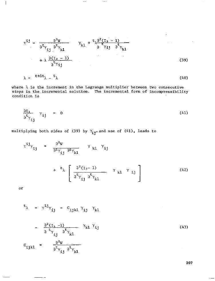
x = - x t + A t x t

where X is the i nc remen t i n t he Lagrange mu l t ip l i e r be tween two consecut ive s t e p s i n t h e . i n c r e m e n t a l s o l u t i o n . The incrementa l form of i n c o m p r e s s i b i l i t y cond i t ion i s

m u l t i p l y i n g b o t h s i d e s of (39) by Yif3 and use of (411, l e a d s t o

or

a 2~ 'ij k l

- - a Yi j a Y U t t

207

C

The fo l lowing scheme may now b e c o n s i d e r e d f o r t h e s o l u t i o n o f incompress ib le materials w i t h o u t t h e n e e d f o r i n t r o d u c i n g t h e unknown Lagrange m u l t i p l i e r . I n t h e p r o c e s s of inc remen ta l so lu t ion , t he last term i n t h e '

r i g h t hand s ide of equat ion (39) i s ignored. A t the end of each increment , t X c an be upda ted f rom r e l a t ion (43 ) . The re is, therefore , no need of t r e a t i n g x a s an independent unknown. No numerical work, however, has b e e n c a r r i e d o u t w i t h t h i s a l t e r n a t i v e p r o p o s e d scheme a t t h i s time.

REFERENCES

1. Herrmann, L.R., "E la s t i c i ty Equa t ions fo r Incompress ib l e and Near ly Incompress ib le Materials by a V a r i a t i o n a l Theorem", A m Jounal , Vol . 3, No. 10, pp, 1896-1900, Oct. 1965.

2. Oden, J.T., "Finite Elements of Nonlinear Continua", McGraw- H i l l , Inc. 1972.

4. Zienkiewicz, O.C., "The F in i t e E lemen t Method" Th i rd Ed i t ion , McGraw-Hil l Book Company 1977.

2 08

Figure 1.- One-d imens iona l s t r e s s - s t r a in r e l a t ion .

'

H IEl

I I ~~ I ~~ *

0.2 0.4 0.6 0.8 1 .o 'd

Figure 2.- V a r i a t i o n of HE with. s t r a i n .

2 09

SOLUTIONS OF CONTACT PROBLEMS BY THE ASSUMED STRESS HYBRID MODEL

Kenji Kubomura System Development Corporation

Theodore H .H . Pian Department of Aeronautics and Astronautics

Massachusetts Institute of Technology

SUMMARY

A method has been developed for contact problems which may be either frictional or frictionless and may involve extensive sliding between deformable bodies. It i s based on an assumed stress hybrid approach and on an incremental variational principle for which the Euler's equations of the functional include the equilibrium and compatibility conditions at the contact surface. The tractions at an assumed contact surface are introduced as Lagrang- ian multipliers i n the formulation. It has been concluded from the results of several example solutions that the extensive sliding contact between deformable bodies can be solved by the present method.

INTRODUCTION

The finite element method has been applied by many authors for solving solid mechanics problems which involve undetermined contact surfaces. They include the relatively simple Hertz contact problem for which there i s no sliding between contact surfaces and the small displacement model can be used [ l , 21. They also include problems involving relative sliding either with friction or i n frictionless conditions [31. Existing solutions are based largely on the conventional assumed displacement finite element model.

The present paper i s based on an assumed stress approach and on an incremental variational principle for which the Euler's equations of the functional include the equilibrium and compatibility conditions at the contact surface. An assumed contact surface is inserted between bodies in contact and i s divided into elements. Contact tractions are independently assumed i n terms of unknown values of such nodes of the contact elements. Thus, a finite element equation includes nodal displacements and nodal contact tractions as unknown. This paper i s to present the variational principle and the corresponding finite element implementation for this problem.

21 1

SYMBOLS

Coordinates before deformation

Displacements defined within an element

Displacements defined along element boundaries

Tractions

Contact tractions

Coefficient of friction

The whole boundary of the body

The contact surface

The portion of the boundary where displacements are prescribed

The portion of the boundary where loads are applied.

Volume

Strains

Stresses

Quantity tangential to the contact surface

Quantity normal to the contact surface

Matrix

Tensor

Prescribed quantity

Quantity pertinent to body A

Quantity pertinent to body B

Quantity pertinent to bodies A and B

Quantity pertinent to element N

incremental auantitv

21 2

I

GENERAL INCREMENTAL ASSUMED STRESS FORMULATION FOR CONTACT PROBLEM

The requirements for contact (the conditions of contact) are as follows:

( 1 ) At the point of contact between two bodies tractions exerted on each other are the same in magnitude and are opposite i n directions.

(2) The normal tractions are compressive and the tangential tractions counteract relative movement of the bodies.

(3) There should be no gap and no penetration of material points at the place of contact.

A B Consider two bodies A and B shown in Fig. 1 with volumes V and V , and boundary

B A B surfaces, a@ and 2V which are composed of portions, S,,- and Sf, and SA and S

These two bodies share a contact surface, S through which they interact. The previously

B U U '

C mentioned conditions of contact i n incremental form are

+ AT^) + (TB + AT B ) = 0 n n

(TB + AT^ ) B S G - + ( T ~ n + AT^) n

21 3

and the signs in Eqs. 3 and 4 are chosen such that tangential tractions on this surface act to restrain the relative movement of contacting points.

A f inite element method which i s based on a variational principle with relaxed continuity requirement at interelement boundaries i s defined as a hybrid model [4]. Boland and Pian [5] have applied an incremental assumed stress hybrid method for large deflection analyses of thin elastic structures. The functional IT that has been derived in the reference [5]i based on the Updated Lagrangian coordinate system i s used as ;base for der iv ing the functional for the present problem.

me

The conditions of no gap and no overlapping on t,he plac%of contact are $traduced into the functional by means of Lagrangian multipliers, T + A T and 7 + A T . The functional K becomes Pmc, i.e.

n n S S

mc

AT. ( AU. - AU. dS -A -40

I I

A +B

s C N s C N

21 4

The Euler's equations of T are C

rnc

On the contact surface S , in addition to Eqs. 5 and 6 cN

(TB n + ATB) n + (7 n + AT n ) = o

Introducing frictional constraint on 7 + A? and 'i +z such that S S n n'

cu

T + A T < + , , T + A T S S - [n -n)

and rearranging Eqs. 11, 12, 13, 14 and 15, results i n Eqs. 1, 2, 3, and 4. Thus, it has been proved that the conditions of contact are Eulers's equations of the functional 7i' C

21 5

These Euler equations are the strain displacement relations, the mechanical boundary condition, the stress equilibrium requirements along the interelement boundaries and the conditions of contact. Since they are only satisfied in an average sense within an increment they cannot be expected to satisfy these conditions i n the usual sense. It is, therefore, necessary to consider a compatibility check, a stress equilibrium check, and a contact check.

It i s seen that Eq. 7 already has al l of these built-in checks. The 5 t h and 6-th integral terms in the functional correspond to the equilibrium check and 7-th term to the compatibility check. Also, the compatibility and equilibrium checks of the contact surface (contact check) are easily identified, the equilibrium check being the 8-th integral term and the compatibility check, the 9-th term.

FINITE ELEMENT IMPLEMENTATION

Since the aim of the present work i s to solve contact problems by the finite element method, expressions arising from nonlinearities, not due to contact, are excluded from equations. A technique for solving these equations, with only contact nonlinearities, wi l l be discussed here.

Neglecting nonlinearities not due to contact, the assumed stress hybrid functional,

77 takes the form mc

3 cN

The stresses AS are expressed in terms of a finite number of stress parameters, A P and the element boundary displacements interpolated in terms of the nodal displacements, CJ, and AZ. Also, coordinates are interpolated in terms of their nodal values. As a solid continuum i s subdivided into elements, the contact surface is also discretized into finite number of elements referred to here as ''contact elements" with "contact nodes. 'I The contact traction J + AI i s interpolated in terms of i t s nodal values, t.

Y

+ N

Thus, interpolatbns otthem are: A z = P a ~ 2 , A: = 5 A:, lJ = q, A = ACJ and 1 + A$ = M i. Substituting these interpolations into Eq. lz,

H

v

Y

and defining the following matrices

R0 L T - T d S , R: N N = \ s h j T * [ ( g A + ) - (GB + gB)]dS

A -E N

IC.

c N

FA = \ M - L d S , F L = M - L B d S 4N " - *

A

C C

JcN JcN

the functional, becomes mcN

21 7

in which S i and 5; result from stress equilibrium checks on S , and on the contact

surface S , and RC , from the init ial mjsmatch checks on S . N n 0

cN N cN

Equation 17 contains three unknown vectors, the incremental stress parameters AZ, the incremental displacements AI, and the contact stresses . Whereas, the vector are independent on the element level, a q and are not. Thus, eliminating AZ from Eq. 17, n' becomes

w

mc

Summing up over a l l elements and !aking the va r ia t i ons of t h e f u n c t i o n a l w i t h respec t to a q and t , resulk in

' W r u

where

K hr = GjN* T tiN - 1 - S N , Q = x(,aN + Q i - Ro ) u -E N * N N

&C K =

Equation 19 represents the total assembled finite element matrix equation.

21 8

I

TECHNIQUE OF ITERATIVE SOLUTION

Once the contacting bodies are adequately constrained such that the inverse of the global stiffness matrix, 5-1 i n Eq. 19 can be calculated, it can be used throughout the iteration procedure. Thus, i n locating the contact surface only K needs to be recomputed i n each iteration. The global stiffness matrix 5 remains constant % uring this process. Even in the case of material and/or large deflection nonlinearities, it i s possible to use a modified Newton-Raphson method; hence the global stiffness matrix 51 may remain constant during this process.

For a two-dimensional problem, before each iteration, the contact surface i s a line, f ixed in the coordinate system, but not to the contacting bodies. Such line i s assumed known i n order to perform the necessary integrals. But if, before the iteration, one has assumed the location of the contact surface and the positions on i t that the contacting nodes of the bodies wi l l occupy, then it would appear that the displacement increment can be specified. Th is i s not the case. Instead, the problem i s solved for the displacement increments and i f the contact surface found therefrom i s not coincident with the one presupposed, a new contact surface location i s calculated, and then an iteration can be followed.

It has been found that the length of the contact element which yields best results i s the same as the length of the contacting side of boundary elements of the bodies. In order to facilitate programming, the nodes of the contact element are chosen to be coincident with those of one of the contacting bodies. As a result of variations i n load, the place of contact changes: thus a vital part of the solution i s to establish a procedure for calculating this change. A tr ial and error scheme i s employed because i t i s virtually impossible to form- ulate a variationalprincipleincluding unknown variables which locate the surface of contact.

The overall strategy for solving the contact problem i s discussed here. First, an increment in the external load or prescribed displacement i s applied. Second, a contact surface i s assumed together with the points on it through which nodes of the bodies contact each other. Also, the types of contact (sliding or non-sliding) at each of the above-mentioned points areassumed .For the initial calculation of the first load increment, the above assumptions are made simply by inspection, and for the first iteration after each new load increment, the converged solution of the previous load step i s used. Third, a l l the necessary matrices are calculated and assembled. At the i-th iteration of the N-th load step, incremental

displacement, AU and contact tractions '(Tk + A T ) are solved from a finite element

matrix equation, Fourth, knowing the total displacement U at the end of,the previous k loading step N-1, the total displacements U + 'A U on the boundary, and contact

tractions (Tk + A? ) are checked to determine i f they satisfy the conditions of contact.

If they do not satisfy these conditions, the location of the assumed contact surface i s modifi'ed and the procedure repeated until they do. Next, a convergence test i s made, and i f the solution i s not convergent, the location of the

I c

k N-1

N-1 k k

I

k

21 9

contact surface i s further modified and the solution procedure repeated.

To determine i f the solution satisfies the conditions of contact, the following assurances are made:

( 1 ) That nodes of either body beyond the last contacting nodes from the previous iteration have not penetrated the other body.

(2) That tractions a t the contacting nodes are compressive. These normal tractions can be calculated by three different methods; (a) from the stress coefficients, (b) from the equivalent nodal forces, and (c) from the contact tractions, $ + A.. Here the last method was used.

(3) That the relationship between normal and tangential contact tractions,

i s satisfied. Depending on which of the above checks, i f any, i s violated, one of the following procedures i s employed to modify the assumed location of the contact surface.

(a) If ( 1 ) i s violated, the contact surface may be extended to include the points at which penetration has occurred.

(b) If (2) i s violated, the contact surface i s reduced by ekcluding nodes at which the tractions are tensile.

(c) If (3) i s violated, sliding i s allowed to occur.

After the conditions of contact are satisfied, a test for convergence can be made by calculating the following quantity:

where AU i s the displacement at the k-th degree of freedom. If R i s less than a precribed quantity, say 0.01, the solution i s considered as converged.

k

EXAMPLE SOLUTIONS

The finite element model and solution scheme are applied to problems of contact between a disk and a semi-infinite half-plane. The overall mesh pattern, the location of

220

the prescribed displacement and relevant dimensions are shown in Fig. 2-a, with the area immediately surrounding the contact surface shown in great detail in Fig. 2-b. The semi- infinite half-plane has been modeled by a finite one with overall dimensions much larger than those of the disk. The basic element used i s four-node quadrilateral element derived by assuming seven P -parameters and I inear displacement distribution along each edge. Five-node and six-node elements are also introduced in transition regions between coarser and finer meshes. Contact tractions along each contact element are approximated by linear interpolations.

Non-Sliding Contact

Problems are solved for the case with both applied loads and prescribed displacements at the top of the disk. In the problems, the ratio of Young's moduli are varied over a range from 1 to and slightly different mesh patterns near the contact surface are used to accornrnoda te'. node-to-node and node-to-internode contacts. Loads or displacements are applied by hethree increments until the length of contact surface becomes about 2.4 mm, For each increment, the converged solutions are reached with three or four iterations. For these solutions, the best results for contact tractions are obtained when calculated from equivalent nodal forces and are compared excellently with the Hertz solution i n a l l cases.

Frictionless Contact With Extensive SI iding

The half disk and the semi-infinite half-plane are also used to demonstrate the capabi l i ty of this forrnulat ion to solve extensive sliding contact problems. Since the contact between the two bodies i s frictionless, the solution i s independent of the path; thus a Hertz solution i s again available for comparison. Solutions are obtained for prescribed displacements at the top of the disk by eight increments. Stress distributions on the p l a n e of contact, for two prescribed displacements, are plotted in Fig. 3 where zero position represents the point of initial contact. It i s seen that the solution agrees almost exactly with that of the Hertz solution. It i s noted that the center of symmetry of the stress distribution moves to the left as the half-disk slides in that direction.

Frictional Contact With Extensive SI iding

The same problem i s again solved here with friction between the disk and the half- plane as an added consideration. No solution to this problem, analytic or otherwise, can be found; thus, results arrived at here wil l be justified by comparison with the results of the previous section and by showing that they satisfy the conditions of contact.

The normal tractions at the contacting nodes between the disk and the half-plane for every 4th displacement increment are shown in Fig. 3 and are compared with those of the frictionless case. Because of friction, i t can be seen that the displacement of the contact surface is retarded. That the normal tractions of the plane and disk are equal i n magnitude and opposite in sign i s also evident i n the figure. This implies that the normal tractions satisfy a condition of contact. A condition of sliding contact requires the ratio between normal and tangential components of tractions to be constant and equal to the coefficient of

221

fr iction . They were approximately verified for all contacting nodes. Finally, the contacting surfaces of the disk and the plane are shown in Fig. 4 along with the locations of the .nodes obtained in previous solutions. It can be seen that friction retards the movement of the contact surface, and as in the previous solution, through averaging over the entire contact surface, the contact condition of no separation or penetration i s satisfied.

C.0NCLUS IO NS

An incremental variational principle and a corresponding finite element formulation have been made for contact problems based on an assumed stress hybrid method. An iterative scheme for the solution has been developed.

Successful applications of the present method for plane elasticity problems have been demonstrated for

(a) Non-sliding problems with node-to-node contact and with node-to-internode contact,

(b) Frictionless contact with extensive sliding, and

(c) Frictional contact with extensive sliding.

The present method should be extended to problems involving material and/or geometrical nonlinearities in addition to contact nonlinearity.

REFERENCES

Tsuta, T. and Yamaji, S . , "Finite Element Analysis of Contact Problem", Theory and Practice in Finite Element Structure Analysis, University of Tokyo Press, 177- 194 ( 1973).

Wilson, E.A. and Parsons, B., "Finite Element Analysis of Elastic Contact Problems Using Differential Displacements", Int. J. Num. Meth. Engng., Vol . 2, 387-395 (1970).

Chan, S. H. and Tuba, I .S., "A Finite Element Method for Contact Problems of Solid Bodies", Int. J. Mech. Sci., Vol. 13, 615-639, (1971).

Pian, T. H .H . , "Finite Element Methods by Variational Principle with Relaxed Continuity Requiremenfll, Variational Methods i n Engineering, Edited by C.A. Brebbia and H. Tottenham, Southhampton University Press, England,

.,

September, Session 1 1 1 , pp. 3.1-3.24, (1972).

Boland, P. L. and Pian, T.H .H ., "Large Deflection Analysis of Thin Elastic Structures by the Assumed Stress Hybrid Finite Element Method", Computers and Structures, Vol. 7, pp. 1-12, (1977).

L 743.6 mm

Figure 2.- Mesh pa t te rn .

223

T R A C T 1 ON (hg/mm) 0- TRACTTON ON HALF- PLANE

600 I (NEGATT E, u= 0.2 1

a" TRACTTON ON VTSK (p=

0 TRACTTON (p= 0 . 0 )

HERTZ SOLUTTON

EIGHT TNCREMENTS DX= - 0 . 4 , VY= -0

-2 .0 - 7 . o 0 1 .0 (mm) X

Figure 3.- Normal t rac t ion on contact surface.

0.2)

. 3

A PLANE (WZTff FRZCTZON) mml X v I I . B 1 I

-0.6 -0.5 - 0 . 4 -0.3 -0.2 - 0 . 1

Figure 4.- Location of nodes.

224

FINITE ELEMENTS FOR CONTACT PROBLEMS IN TWO-DIMENSIONAL ELASTODYNAMICS

Thomas K. Zimmermann IPEN, Swiss Federal Institute of Technology, Lausanne, Switzerland

Wing Kam Liu Div. of Eng. and Applied Science, CALTECH, Pasadena, USA

SUMMARY

This article summarizes some aspects of research in progress for developing finite element methods for contact problems. We propose a new"finite element approach" for contact problems in two-dimensional elastodynamics. Sticking, sliding and frictional contact can be taken into account. The method consists of a modification of the shape functions, in the contact region, in order to involve the nodes of the contacting body. The formulation is symmetric (both bodies are contactors and targets), in order to avoid interpenetration. Compati- bility over the interfaces is satisfied. The method is applied to the impact of a block on a rigid target. The formulation can be applied to fluid-structure interaction, and to problems involving material nonlinearity. The extension to three dimensions presents additional difficulties, but it is possible.

INTRODUCTION

The approach presented in this article was developed while trying to simulate the movement of a gas bubble in a liquid. The original idea was to introduce the compatibility of the velocities over the gas-liquid interface via a constraint equation and to handle it by the Lagrange multiplier method. In a second step, the Lagrange multiplier method was replaced by a penalty method, which is easier to implement. In both cases, the constraint equation is a geometric relationship between gas and liquid velocities. No local remeshing was performed; the bubble and liquid meshes were simply superposed. This resulted in poor pressure fields along the interface. Looking for an improvement of this situation, remeshing appeared as the best but also the most cumbersome solution. Alternatively, a modification of the shape functions appeared to have the advantages of remeshing, without its inconveniences. This latter approach is described herein as it is applied to contact problems in two-dimensional elastodynamics. Frictional contact results in an exchange of momentum between the two contacting bodies, and can be realised by direct introduction of a contribution of the contactor's velocity into the target's equation of motion. This is conveniently done by means of a modification of the shape functions, as described in the next paragraphs.

225

The proposed approach has the advantage, as compared t o t h e Lagrange mul - t i p l i e r method, of maintaining a c o n s t a n t s i z e of t h e l i n e a r s y s t e m t o be solved. Compared t o a penalty method, it has the advan tage t ha t we ge t au to- matic c o m p a t i b i l i t y of t h e f i e l d variables o v e r t h e i n t e r f a c e . When t h e formulat ion i s symmetric ( i . e . , both bodies are targets and c o n t a c t o r s ) , i n t e r p e n e t r a t i o n i s t o t a l l y a v o i d e d .

MODIFIED SHAPE FUNCTIONS FOR QUADRILATERAL FINITE ELEMENTS

Figure 1 shows a two-dimensional contact problem. Node C contacts e lement (1-2-3-4) o f t h e t a r g e t a n d from then on c o n t r i b u t e s t o i t s shape func t ions . We s ta r t from t h e i n i t i a l 4-nodes i n t e r p o l a t i o n f u n c t i o n

4 v = 1 N, va

with Na = 0.25 (1+ sign(c,) g ) ( l + s i g n ( - q , ) q ) ( 2 )

where 5 , 7 a r e l o c a l c o o r d i n a t e s , a n d v a r e t h e v e l o c i t i e s . I n o r d e r t o take t h e c o n t r i b u t i o n o f p o i n t C (node 5 ) i n to accoun t , we modify t h e i n t e r p o l a t i o n f u n c t i o n as fol lows :

5 v = 1 Nl V,

a= 1 N o t i c e t h a t from a g loba l po in t o f v iew there i s no new node appearing.

Obviously, a "hat shape funct ion" a t node 5 i s t h e most adequate for our pu rpose . Th i s y i e lds au tomat i c compa t ib i l i t y o f t he ve loc i t i e s at t h e i n t e r f a c e , if a symmetric formulation i s used . Fur ther , we want t o a c c o u n t f o r t a n g e n t i a l s l i d i n g w i t h f r i c t i o n a t the con tac t po in t . The re fo re , we in t roduce a f a c t o r p which a l lows the shape funct ion a t node 5 t o va ry i n ampl i tude be tween 0 and 1, which w i l l l e a d t o a p a r t i a l exchange of momentum. The r e su l t i ng shape func t ions are (assuming C i s on s i d e 7 = + 1) :

and * N, = N, - a, N: a = 1-4

with a, = 0.5 ( l+s ign 5, g 5 ) The loca l coo rd ina te s o f C are (E ,l). We can a l so assume, wi thout res t r ic -

t i o n , t h a t t h e c o n t a c t p o i n t i s a s s o c i a t e d w i t h l o c a l c o o r d i n a t e s ( 0 , +I) , N* 5 5

2 26

This shape funct ion i s shown on f igure 2. Observe t h a t N 5 ( E 5 , T 5 ) does not vanish a t node 5 when p# 1, but Na = 1 is preserved.

I n the sequel , w e s epa ra t e no rma l (n ) and t angen t i a l ( t ) d i r ec t ions and t h e r e f r o m t h e f o l l o w i n g t y p i c a l p o s s i b l e s i t u a t i o n s .

a. p n = 1, pt = 0 , c o r r e s p o n d s t o f r i c t i o n l e s s s l i d i n g i n the t a n g e n t i a l d i r e c - t i o n a n d s t i c k i n g i n t h e normal direct ion. This y i e l d s :

N = Na ( a = l - - 5 ) , t h e s t a n d a r d 5-nodes i n t e r p o l a t i o n

func t ion ,

N = N ( a = l - b ) , t he s t anda rd 4-nodes i n t e r p o l a t i o n t a

func t ion .

* n

*

c . p n = l , pt ~ ] 0 . 1 [ t h i s a c c o u n t s f o r f r i c t i o n a l s l i d i n g .

Since pdepends on o r i e n t a t i o n , w e in t roduce a second order tensor , which w e need i n o r d e r t o d e f i n e s t r a i n rates and s t r e s s e s i n g l o b a l c o o r d i n a t e s .

I n a loca l o r thogona l frame t a n g e n t i a l t o t h e t a r g e t s u r f a c e we wr i te

where t h e s u p e r s c r i p t s T and C s t a n d f o r t a r g e t a n d c o n t a c t o r , r e s p e c t i v e l y , a n d t h e s u b s c r i p t s n and t fo r no rma l and t angen t i a l .

t Equation ( 7 ) d e f i n e s t h e c o n t r i b u t i o n o f node 5 ( c o n t a c t o r ) t o t h e t a r g e t v e l o c i t y w h i l e t h e t r u e l o c a l v e l o c i t y , a t C y i s given by

2 27

where t

and [ N,"] i s de f ined as fol lows ti

The mat r ix En i s diagonal when d e f i n e d i n a l o c a l r e f e r e n t i a l , t a n g e n t i a l t o t h e c o n t a c t s u z f a c e . I t does not induce a coupl ing of the normal and tangen- t i a l components , bu t th i s would no t be t rue in a g l o b a l r e f e r e n t i a l . We can, t h e r e f o r e , e s t a b l i s h t h e s t i f f n e s s i n t h i s l o c a l r e f e r e n t i a l a n d r o t a t e t h e element matr ix before we assemble the e lements . Al te rna t ive ly w e can make t h e d e r i v a t i o n i n a g loba l coord ina te sys tem.

In p rac t i ce , t he who le e f fo r t e s sen t i a l ly r educes t o minor changes i n t he shape func t ion rou t ines .

TRANSIENT SOLUTION PROCEDURE

Search Algorithm

We need to de t e rmine a t each time s t e p t h e l o c a t i o n o f e a c h node of each body i n t h e c o n t a c t zone w i th r e spec t t o t he mesh o f t he o the r one . For t h a t purpose a connec t iv i ty ma t r ix i s e s t a b l i s h e d i n t h e i n p u t p h a s e ; t h i s m a t r i x l i s t s a l l elements connected to each e lement . Assuming t h e time s t e p t o b e small, w e memorize t h e p r e v i o u s p o s i t i o n o f e a c h node (by an element number), and search for i t s new pos i t i on i n ad j acen t e l emen t s . A 2-dimensional search pa th i s shown on f i g u r e 3. Once t h e new p o s i t i o n i s known, w e modify t h e shape func t ions o f the t a rge t e lement as d e s c r i b e d i n t h e p r e v i o u s p a r a g r a p h and compute t h e u p d a t e d s t i f f n e s s e s .

t T as supe r sc r ip t o f a m a t r i x s t a n d s f o r t r a n s p o s e tt a depends on t h e l o c a l c o o r d i n a t e o f t h e f i f t h node a

228

Predictor-Corrector Algori thm

We adop t he re an exp l i c i t p red ic to r - co r rec to r a lgo r i thm, de f ined by t h e fo l lowing equat ions , at t i m e s t e p ( n + 1) (see re f . 1, 2 f o r detai ls) .

Equations (16) and (17) are p r e d i c t o r e q u a t i o n s ( u p p e r t i l d a ) , (18) and (19) a r e c o r r e c t o r e q u a t i o n s , ( 2 0 ) t o ( 2 2 ) are i n i t i a l c o n d i t i o n s , and N i s a nonl inear a lgebra ic opera tor? . The implementation procedure can be found in ( r e f . 1).

If f r i c t i o n a l c o n t a c t o c c u r s , w e n e e d i n a d d i t i o n a p red ic to r equa t ion for pn+ . Because of lack of space, t h i s i s not developed here . For t h e time be ing

we a i o p t

-

NUMERICAL RESULTS

The ana lys i s o f an impact o f a rec tangular b lock on a r i g i d s u r f a c e i s performed (see r e f . 3, for comparison). Figure 4 shows t h e mesh. The data a r e

dens i ty p = 0.01

modulus o f e l a s t i c i t y E = 1,000

P o i s s o n ' s c o e f f i c i e n t v = 0 . 3

dimensions L . w = 9.4 t i m e s t e p A t = 0.002725

t If variables are t o b e memorized a t e l emen t i n t eg ra t ion po in t s , as o f t e n i n nonlinear problems, remember t h a t t h e s e are moving when node 5 moves.

229

Newmark parameters ( e x p l i c i t p r e d i c t o r - co r rec to r a lgo r i thm)

y = 0 . 5 p = O . 2 5

i n i t i a l v e l o c i t y vo = 1

wave v e l o c i t y C, = ( [ E ( l - v ) ] / [ ( l + V ) ( l - 2 V ) - p]}Oe5 = 366.9

The time s t e p i s d e f i n e d b y t h e t r a n s i t time f o r a d i l a t a t i o n a l wave t o c ros s one element. The impact t akes p lace a t t = 0. F r i c t i o n l e s s c o n t a c t i s assumed (p = 0 ) . This i s in t roduced via i so l a t ed nodes , as shown on f i g u r e 4a. For t h e p u r p o s e o f t e s t i n g t h e new formulat ion, both node-to-node and dis t inct nodal pos i t ions are t e s t e d a n d y i e l d t h e same results.

t

The a n t i c i p a t e d s o l u t i o n i s shown on f i g u r e 4b. Th i s exac t so lu t ion has two constant zones separated by the d i l a t a t i o n a l wave f ront emanat ing f rom the i n i t i a l i m p a c t . The c i r c u l a r wave f r o n t i s a result o f r e f l e c t i o n s o f f t h e free boundary.

During t h e e a r l y s t e p s o f t h e c o m p u t a t i o n , stresses i n zone I1 are obta ined f rom the impulse equat ion appl ied to a one-d imens iona l s i tua t ion ( U = c - p - v 0 ) S t r e s s results shown on figure 5 .a c o n f i r m t h e v a l i d i t y o f t h e new approach. Some overshoot appears, however, in the s t r e s s results o f t h e l o w e s t row o f e lements , p robably due to the absence o f a d i s c r e t e i m p a c t c o n d i t i o n i n t h e algori thm. The deformed configuration at t = 0 . 0 2 1 8 s . i ~ shown on f i g u r e 5b.

CONCLUDING REMARKS

A new approach to con tac t p rob lems i nvo lv ing f r i c t ion i n t .wo-d imens iona l elastodynamics i s p r o p o s e d i n t h i s a r t i c l e . The b a s i c i d e a o b v i o u s l y shows some ana logies wi th loca l remeshing techniques , l ike the one p roposed in ( re f . 4 ) . The t r e a t m e n t o f f r i c t i o n v i a m o d i f i e d s h a p e f u n c t i o n s seems similar t o t h e l i n e s o f t h i n k i n g a d o p t e d i n ( re f . 5 ) for the treatment of shock waves.

The proposed formulation i s symmetric (both bodies are contactor and tar- g e t f o r e a c h o t h e r ) a n d satisfies c o m p a t i b i l i t y o f v e l o c i t i e s o v e r t h e c o n t a c t i n t e r f a c e (when poss ib le ) , thus avoid ing in te rpenet ra t ion . Comple teness o f the modified elements remains satisfied. Although no de ta i led compar ison wi th d i f - ferent approaches has been made as ye t , t he fo l lowing advan tages can be men- t i oned : c o n s t a n t s i z e o f t he sys t em o f equa t ions (no t t rue f o r local remeshing or Lagrange multiplier approach, important i f a n i m p l i c i t s o l u t i o n i s performed) and i n t e r f ace compa t ib i l i t y (no t t rue i n gene ra l fo r Lagrange mu l t ip l i e r s o r pena l ty methods ) .

The ex tens ion o f t he method to s eve ra l con tac t ing nodes pe r e l emen t i s poss ib l e , bu t it i s n o t t r i v i a l . The e x t e n s i o n t o c o n t a c t g - o b l e m s i n t h r e e dimensional space and inclusion problems in 2-D i s p o s s i b l e , b u t a t t h e c o s t o f l o s i n g i n t e r f a c e c o m p a t i b i l i t y . As already ment ioned , nonl inear ana lys i s may p r e s e n t m i n o r d i f f i c u l t i e s b e c a u s e o f t h e f a c t t h a t i n t e g r a t i o n p o i n t s c a n move.

230

I

Further research i s needed on the p red ic to r a lgo r i thm fo r s l i d ing w i th f r i c t ion and impact-release conditions have to be added.

O u r main e f f o r t , at present , i s directed towards testing the approach i n problems involving friction.

231

REFERENCES

1. T.J.R. Hughes, K.S. Pister, R.L. Taylor : Implicit-explicit finite elements in nonlinear transient analysis. FENOMECH 79 Symposium Proceedings, Stuttgart, West Germany, 1978.

2. T.J.R. Hughes, W.K. Liu : Implicit-explicit finite element in transient analysis. J. of Applied Mechanics, Vol. 45, 371-378, 1978.

3. T.J.R. Hughes, R.L. Taylor, J.L. Sackman, A. Curnier, W. Kanoknukulchai : A finite element method for a class of contact-impact problems. computer Methods in Applied Mechanics and Engineering, No 8, 249-276, 1976.

4. P. Cundall, Joaquim Marti, Peter Beresford, Nigel Last, Margaret Asgian : Computer modelling of jointed rock masses, Dames and Moore R.eport NTIS N-78-4, Los Angeles, 1978.

5. L.C. Wellford, J.T. Oden : Discontinuous finite element approximations for the analysis of shock waves in nonlinearly elastic materials. J. of Computational Physics , No 19, 179-210, 1975.

232

Figure 1.- Contact problem.

Figure 2.- Modified shape functions.

Figure 3.- Search path.

233

( a ) F i n i t e element mesh.

1

I

+X

( b ) Wave front diagram.

Figure 4. - Impact of rec tangular b lock on a r i g i d s u r f a c e .

234

( a ) S t r e s s r e su l t s .

T'

+X

( b ) Deformed mesh.

Figure 5.- S t r e s s r e s u l t s and r e s u l t i n g deformed mesh.

235

INELASTIC BEHAVIOR OF STRUCTURAL COMPONENTS*

Noor Hussain, K. Khozeimeh and T. G. Toridis School of Engineering and Applied Science

The George Washington University Washington, DC 20052, USA

STJMMARY

The objective of this paper is to develop a more accurate procedure for the determination of the inelastic behavior of structural components. For this purpose, the actual stress-strain curve for the material of the structure is utilized to generate the force-deformation relationships for the structural elements, rather than using simplified models such as elastic-plastic, bilinear and trilinear approximations.

Force-deformation curves in the form of universal generalized stress- strain relationships are generated for beam elements with various types of cross sections. In the generation of these curves, stress or load reversals, kinematic hardening and hysteretic behavior are taken into account. Intersections between loading and unloading branches are determined through an iterative process.

Using the inelastic properties determined in this study, the plastic static response of some simple structural systems composed of beam elements is computed. Results are compared with known solutions, indicating a considerable improvement over response predictions obtained by means of simplified approximations used in previous investigations. The application of this procedure to the dynamic load case is currently in progress.

INTRODUCTION

Structural systems analyzed and designed for traditional loads and materials have been observed to undergo inelastic deformations when excessive load conditions are experienced. It is, therefore, an established fact now that inelastic deformations do occur in structures and are considered in the analysis in order to produce more economical and safe designs. For example, a generally accepted philosophy in the seismic analysis and design of structures is that.a structure should remain elastic during earthquakes of small intensity that' occur frequently; it should undergo limited plastic deformations during earthquakes of moderate intensity; however, it may undergo large plastic deformations but without major collapse during earthquakes of relatively high intensity that occur infrequently.

*This study has been partially supported by the National Science Founda- tion Research Grant No. PFR-79-16263.

237

At the same time, advances in naval, aerospace and nuclear reactor technology has led to the use of new materials such as stainless steel, alloys of aluminum and nickel, reinforced plastics, etc. The stress-strain curves for these materials are generally nonlinear. Therefore, an economical design of structures composed of such materials requires an accurate knowledge of the magnitude and distribution of the stresses and strains, as well as, the displacements. In all cases the effect of nonlinearities must be considered in the analysis.

In the study of the inelastic behavior of structures various idealizations to the actual stress-strain curves or force-deformation relations have been employed. The most extensively used model is the elastic perfectly plastic representation, principally due to its simplicity. When unloading occurs, this model neglects the strain hardening and Bauschinger effects. In general it produces conservative results and is mostly suitable for mild steel structures. Bilinear models with a nonzero slope for the inelastic branch have also been used widely. These models allow for the consideration of strain hardening effects (both isotropic and kinematic) due to loading and unloading cycles arising from static and dynamic loads. A trilinear model has also been used to simulate the stress-strain relationship of the material under static loads.

Simplified models often perform satisfactorily in predicting the inelastic behavior of special classes of structures. However, for general types of structures, an accurate representation of the stress-strain or force- deformation properties are needed for both the loading and unloading branches in the form of curvilinear or multilinear (piecewise linear) relations that follow as closely as possible the actual behavior of the system.

In the present study an accurate procedure is considered for the determination of the inelastic behavior of structural components. For this purpose, the actual stress-strain curve for the material of the structure is utilized to generate the force-deformation relationships for the structural elements, rather than using simplified models, such as elastic-plastic, bilinear and trilinear approximations. Applying this process to frame type structures, force-deformation curves in the form of universal generalized stress-strain relationships are generated for beam elements with various types of cross sections. In the generation of these curves stress or load reversals, more realistic strain hardening properties and hysteretic behavior are taken into account. Intersections between loading and unloading branches are determined through an iterative process. Based on the rather accurate force-deformation relationships of the individual elements, the governing equations for the structural system are established and used to compute the inelastic response of the structure.

238

GOVERNING EQUATIONS

Application of the Hamiltonian Principle to discrete systems in the context of the finite element method yields the basic dynamic equations governing the behavior of the structural systems. In matrix form these equations can be expressed as (ref. 1)

where [m] = consistent mass matrix of the structural system.

[K] = elastic stiffness matrix of the structural system.

[K ] = geometric stiffness matrix of the structural system. G

(9) = vector of displacements at the structural degrees of freedom.

{ G > = vector of accelerations at the structural degrees of freedom.

{F} = generalized nodal force vector corresponding to externally applied loads.

{F > = equivalent generalized nodal force vector due to plastic 0

strains, computed in accordance with the initial stiffness method.

In case of static loading the above equations take the form of

([K] + [KG]) {q} = {F} + {Fo>

PLASTICITY RELATIONS

Stress-Strain Curve

An experimentally determined virgin curve of the material is in general curvilinear. Starting with the experimental stress-strain data analytical expressions can be obtained to represent this data. Such expressions can be in the form of algebraic or other types of polynomials, exponential functions, or the widely used curvilinear relationship known as the Ramberg-Osgood approximation represented by

E = ; [1++) R- 1 3

239

in which E and u are the unit strain and unit stress, respectively, E represents the modulus of elasticity, denotes the yield stress of the material and D and R are real constants to “x e determined. However, this relationship is not explicit in stresses and, therefore, numerical procedures are needed to find the stresses corresponding to given strains. On the other hand, if the stress-strain data cannot be represented by an analytical expression, the curve is approximated by a series of line segments given by

where, (U<,E:) are the stress-strain values at the beginning of the ith segment and ki+l 1s ;he slope of the line segment between the points (ai ,E .) and (‘i+l, &i+l

+ ) expressed as 1

a - u - E

i+l i - - ki+l , i = 0,1,2, . . . , (n-1)

where n is total number of segments used to approximate the curve.

Moment-Curvature (Force-Deformation) Relationship

Figure 1 shows a general elasto-plastic doubly symmetric cross section of a beam member. A linear strain distribution over the depth of the cross section up to ultimate behavior is assumed. Tensile stresses are considered positive and curvatures causing positive strains at bottom fibers are also positive. The x- and y-axes are the principal axes and the z-axis is the geometric centroidal axis of the cross section. The bending moment acting on the cross section is the sum of moments of the stresses acting on the cross section about the geometric centroidal axis, i.e.

M = J G ydA

A

in which dA is an element of area. The integration is carried over the elastic and plastic parts of the area. Usually the stress-strain curve of the material cannot be represented explicitly for stresses; therefore, a numerical integration procedure is employed. For this purpose the section is divided into a series of rectangular slices, and the contribution of each slice to the moment acting over the cross section is found. Before indicating the details necessary for accomplishing this, certain definitions need to be established as follows. If cy, and a are the yield strain, ultimate strain and yield stress, respectively, as observed in a tension test on a material and h is the distance to extreme fibers from z-axis, then

Y

240

M = u I / h = u S Y Y Z Y

where My, I,, S are t h e y i e l d moment, moment of i n e r t i a and section modulus of t h e s e c t i o n , r e s p e c t i v e l y . The y i e ld cu rva tu re 4 is obtained f rom

Y I$ = M /E I,

Y Y Based on the assumption of a l i n e a r s t r a i n d i s t r i b u t i o n o v e r t h e c r o s s s e c t i o n of t h e member, t h e u l t i m a t e c u r v a t u r e I$ is given by

U

4, - EU/h -

In the p resent s tudy the curva ture range be tween +y arid O u i s d i v i d e d i n t o a s u i t a b l e number of i n t e r v a l s t o g i v e enough d a t a p o i n t s t o f i t a curve. The s t r a i n a t t h e c e n t e r of i t h r e c t a n g u l a r s l i c e , assumed to be un i fo rmly d i s t r i b u t e d o v e r t h e s l i ce , cor responding to a cu rva tu re va lue 4 is given by

j

where yi i s t h e d i s t a n c e t o t h e c e n t r o i d of t h e i t h r e c t a n g u l a r s l ice from the c e n t r a i d a l a x i s of t h e c r o s s s e c t i o n . The s t r a i n ~i i n t h e i t h s l ice d u e t o curva ture +j, a t t h e j t h d i s c r e t e p o i n t a l o n g t h e member, is used to de t e rmine t h e stress u i assumed t o act un i fo rmly ove r t he en t i r e s l ice , from t h e stress- s t r a i n r e l a t i o n s h i p as d i scussed p rev ious ly . I f Ai is t h e area of t h e i t h s l i ce , t h e f o r c e a c t i n g on t h e i t h s l i ce is given by

The moment of t h e f o r c e a b o u t t h e n e u t r a l a x i s is obtained from

By summing o v e r t h e t o t a l number of s l ices used t o model t h e c r o s s s e c t i o n , t h e t o t a l i n t e r n a l moment M on the c ros s s ec t ion co r re spond ing t o a cu rva tu re is expressed as j j

NS NS M = C M i = C IS A i y i j i=1 i= 1 i

where NS is number of sl ices and j r ep resen t s a t y p i c a l d i s c r e t e p o i n t a l o n g t h e member. S i m i l a r l y t h e t o t a l i n t e r n a l axial f o r c e P a t t h e c r o s s s e c t i o n due t o a p r e s c r i b e d s t r a i n f i e l d E is obtained from

NS

i= 1 P = C ui Ai

241

Equations (13) and (14) directly yield force P and moment M corresponding to a prescribed deformation field. However, to get the deformation corresponding to a given load history, equations (13) and (14) have to be solved iteratively. The moment curvature data generated through the use of equation (13.) is then presented explicitly for curvature by a polynomial of the type

N

i=l 4 = M/EI + c ci M' (15)

where C are the polynomial coefficients to be determined and N is degree of the polynomial. Alternatively, an equation of the Ramberg-Osgood type. i

can be fitted in which D and R are the real constants to be determined.

Normalized Moment Curvature Relationship

The moment-curvature data generated from Eq. (13) is normalized by using the quantities M and 4 so that

Y YY - M = M/M

Y (17)

where fi and 5 are normalized moment and normalized curvature, respectively. The normalized curvature is then separated into its elastic and plastic components $ and 5p, respectively, so that solving for 5 e P

-

Since $ = M/EI, based on equation (17) the normalized elastic curvature is written in the form e

Based on the normalized plastic components of curvature computed from equation (19) , a polynomial of the form

N $p = C di ki

i=O

-

is then fitted to approximate the data, where the d ' s are constants to be determined through regression analysis. Alternatively, an equation of the type i

242

+ P = D M -R

is also used to represent the data. The real constants D and R are determined by taking the logarithmic form of Eq. (22), so that

In 5, = In D + R In ii (23)

This is an equation of a straight line. Constants D and R are determined from linear regression analysis using the data for In 5 and In fi.

P

Using equations. (191, (211, and (221, the following moment-curvature relations can now be formulated

- $=ii , ii<1 (24)

Slope of Generalized Stress-Strain Curve

A universal stress-strain curve usually represents the relationship

between I$ and fi expressed by Eqs. (21) or (22). Rewriting these equations in differential form and solving for the slope E2 yields

-P

If a smooth analytical expression to fit the $ - M data is not possible within tolerable limits of accuracy, the slope E of the universal stress-strain curve is obtained as a series of approximate tangents drawn at discrete points representing the data, i.e.

-P

2

243

where i and if-1 are typical discrete points.

In eqs. (21), (22) and (24)-(29) the cross section is assumed to be subjected to a bending moment about the centroidal axis. However, in practical cases, structural elements are generally subjected to stress resultants acting in different directions. To extend the applicability of the above procedure, it is assumed that similar relationships exist between the effective stress f* and effective strain O* in a multi-axial stress case. The function f* in normalized form is also identisied with the yield function.

Yield Function

When stress resultants in normalized form (instead of unit stresses) are considered to be generalized stresses in the context of plasticity theory, yielding at any section of a member is then assumed to occur when the critical combination of generalized stresses initiate inelastic deformations at that section. The yield function is expressed by an equation of the form

where Qi are the generalized stresses and Y is the initial yield value. To make the yield function independent of the cross section, the yield function equation is derived in terms of normalized (dimensionless) force parameters. A force component is normalized by its corresponding characteristic value (usually the value at first yield). In normalized form equation (30) takes the form of

For a space frame member the cross section is subjected to a generalized force vector S having 6 components, so that

{Px, vyy VZY M x M y y M ) z

where

P = axial force X

vy, vz = direct or transverse shear forces

Mx, My = Bending moments

MZ = Twisting or torsional moment

244

Each of these forces influence the yield behavior at a cross section and the inelastic response depends upon the interaction between them. In the past, elliptical, parabolic, spherical (ref. 2) and other forms of yield functions have been used in inelastic analysis of structures. In the present study a spherical yield function is used as fndicated below

[(&f+(+f+(!k) 2 + ( " ) 2

ox ox Moz

in which P denotes the normalized yield value which may change during straining and P M and M are the characteristic values of axial force,

torsional moment, and bending moments about y and z axes, respectively. Similar expressions can be written for a plate element (ref. 1).

ox' MOx9 oy 0 2

The above yield function can be used in conjuction with an average force model (refs. 1, 3) which assumes that an element undergoes plastic deformations if the loading function f* determined from average values of stress resultants acting at the member ends exceeds the current normalized yield value.

Flow Rule

A flow rule expresses the relationship between plastic strains and stresses. In the present study rather than solving the flow equations rigorously in terms of stress resultants, an approximate procedure (refs. 1, 3) is employed. In this method if f* is the plastic potential at the end of

a load increment in dynamic analysis (.computed using member forces P

obtained from an elastic analysis), then the increment of plastic potential df* for an element already undergoing fnelastic deformation is obtained from the equation

est i est

1

* * * dfl - - - fest fprev

where f is the plastic potential at the end of previous load or time

increment. For a transitional element the equation for the increment of plastic potential is of the form

* pr ev

* * dfl = f - f * est 0

( 3 4 )

( 3 5 )

where f * is the initial yield value. 0

245

As shown in detai’l in reference 1, the correct value of the plastic potential increment df* can be computed from the relation

L

The current corrected value of the plastfc potential f is thcn obtained as * curr

f* = f *

curr prev + df

for an element already undergoing plastic deformations and * *

0 curr = f + df*

(37 )

for an element entering the plastic range.

With the known value of the plastic potential f , the final values of member (element) forces are computed by a proportioning procedure represented as (refs. 1, 3)

*

pi - Pi curr - curr est <*

(39)

The overall numerical procedure utilized in the computation of the element and structural responses is the same as the one outlined in references 1 and 2.

NUMERICAL RESULTS

To determine the feasibility of the proposed method, two structures for which results are available in the literature were analyzed and the results were compared with the works of other investigators.

Example 1 - The first example considered consists of the simply supported beam with the I cross-section and material property, as shown in figure 1. The given stress-strain curve corresponds to material B as defined by Chajes (ref. 4 ) who had originally studied this structure. As in the case of the above reference, the stress-strain curve is idealized by a bilinear relationship. This is then utilized to obtain the moment curvature and the normalized universal stress-strain curves, as depicted in figure 2.

246

Subsequent ly , the response of beam when s u b j e c t e d t o e i t h e r a concent ra ted load a t i t s midspan o r a un i fo rmly d i s t r ibu ted l oad ove r i t s e n t i r e l e n g t h is obtained. It should be ment ioned that Chajes ( ref . 4) has presented a "closed-form" s o l u t i o n f o r t h e d e f o r m a t i o n c h a r a c t e r i s t i c of the midspan of t h e beam when s u b j e c t e d t o a concentrated load. However, h i s s o l u t i o n i s based on the assumption that only the f langes resist the bending moment. I n f i g u r e 3 are shown the de f l ec t ion r e sponses of t h e midspan as o b t a i n e d i n t h i s s tudy as w e l l as t h a t r e p o r t e d i n r e f e r e n c e 4 . As can be observed, close agreement between the two sets of d a t a is exhib i ted .

Example 2 - As a second example, a p in-based por ta l f rame s tud ied , bo th t h e o r e t i c a l l y and experimentally, by Takahashi and Chiu (ref. 5) i s analyzed. The s t r u c t u r e c o n s i s t s of W12X27 sect ions, arranged to deform around their s t rong axes . The geometry of the structure and i ts loading are shown i n f i g u r e 4a. The i d e a l i z e d s t r u c t u r e and the equiva len t nodal loading is shown i n f i g u r e 4b. Note t h a t t h e e f f e c t of t he g i rde r dep th has been t aken i n to account by in t roduc t ion of an addi t iona l equiva len t load and a bending moment a t the top o f the loaded co luw. In the ana lys i s , a curve is f i t t e d t o t h e s t r e s s - s t r a i n r e l a t i o n f o r t h e m i l d steel with an average yield stress of 255 MN/m2 and modulus of e l a s t i c i t y of 203. 5X103 MN/m2. This i s then used as a b a s i s f o r d e t e r m i n a t i o n of moment-curvature re la t ionship for the s t ructure . I n f i g u r e 4 c is shown the ho r i zon ta l de f l ec t ion r e sponse of t he t op of t h e unloaded column. Again, c l o s e c o r r e l a t i o n is observed.

REFERENCES

1.

2.

3.

4.

5.

Khozeimeh, K . , " I n e l a s t i c Response of Beam-Plate Assemblages Subjected t o S t a t i c and Dynamic Loads," d i s s e r t a t i o n p r e s e n t e d t o t h e George Washington University, a t Washington, D . C . , i n 1974, i n p a r t i a l f u l - f i l l m e n t of the requirements for the degree of Doctor of Science.

Morris, G. A . , and Fenves, S . J . , "Approximate Yield Surface Equations," Jou rna l of the-Eng-ineering Mechanics Division, ASCE, Vol. 95, No. EM4, Proc. Paper 6741, Aug., 1969, pp. 937-959.

Khozeimeh, K . , and T o r i d i s , T.G., "Models f o r I n e l a s t i c Response of Beam- P l a t e Assemblages," Journal of the Engineering Mechanics Division, ASCE, Vol. 104, No. EM5, October 1978, pp. 1001-1014.

Chajes, A . , " Ine la s t i c Def l ec t ion o f B e a m s , " Jou rna l of t h e S t r u c t u r a l Div is ion , ASCE, Vol. 94, No. ST6, Proc. Paper 6012, June, 1968, pp. 1549- 66.

Takahashi, S. K . , and Chiu, R. H . , "S ta t ic and Dynamic Behavior of Pinned-Based P o r t a l Frames," NCEL TR336, Feb., 1965.

247

2 48

r - _I

Figure 1. - Geometrical and

Moment-Curvature

Curvature ( I O - Z / ~ )

F igure 2. - Moment-curvature and

560

Strain (10-3 crn/cm)

material p r o p e r t i e s .

1.4

Clu 1.2

1.0

0.0 0.5- 1.0 $p

Universal Stress-Strain

u n i v e r s a l s t r e s s - s t r a i n c u r v e .

I 111111

I l l

1254 mm +t- 8@ 63.5 mm 1254 mm

300

2 50

200

150

100

50

- Ref. 4

0 Present

3 6 9 12 15 18 Deflection (mm)

(a) Point load.

~~~

5.5w 7@ 3w 5.5w

203 m 8 @ 7.62 mm

3

1200

1000

800

600 - Ref. 4 - 400

200

0 Present

Deflection (mm)

(b) Uniformly dis t r ibuted load.

F igu re 3 . - Loading and mid-span de f l ec t ion r e sponse .

2 49

r- 3.657 m ln

160

h 120 6 1

B v

a0 3 a m 2 40

(a) Actua l frame.

+ 4@ 0.91441~ "c1 I

c t 8 4 . 2 4 ~ - 8 4 . 2 4 ~

8 4 . ~ 4 ~ - ah. 24W -

E 4 m -3

0

W ln

(b) Ideal ized f rame.

0 0 Presen t study

- Experimental (Ref. - - Theore t ica l (Ref .

0 0 Presen t study

- Experimental - - Theore t ica l (Ref .

4 a 12 16 20 24 2a

( c ) Hor izon ta l de f l ec t ion of j o i n t C (cm).

Figure 4 . - Pin-based p o r t a l f r a m e .

250

NONLINIXR FINITE ELEMENT ANALYSIS - AN ALTERNATIVE FORMlTLATION

S i l v i o Merazzi" Ecole Polytechnique Fgdgrale de Lausanne, Switzerland

SUMMARY

A geometrical nonlinear analysis based on an a l t e rna t ive de f in i t i on o f s t r a i n i s presented. Expressions for strain are obtained by computing t h e change in l ength o f the base vec tors i n the curvil inear element coordinate system. The isoparametric element formulation i s assumed i n the global Cartesian coordinate system. The approach i s based on the minimizat ion of the s t ra in energy, and the resul t ing nonl inear equat ions are solved by the modified Newton method. Integrat ion of the first and second variation of the s t r a in energy i s performed numerically in t he ca se o f two- and three-dimensional elements. Ap- p l i c a t i o n i s made t o a simple long cantilever beam.

INTRODUCTION

The non l inea r f i n i t e element formulation described here represents a par t of the development of t h e BASIS f i n i t e element analysis system (ref. 1). The basic idea w a s t o combine l i n e a r and nonlinear behaviour in o rde r t o dea l more e f f i c i e n t l y w i t h s t r u c t u r a l a n a l y s i s . Thus, nonlinear elements had t o be developed which f i t into an existing system without loss of general val idi ty . The Lagrange formulation has therefore been chosen (ref. 2 ) , expressing the displacement variables directly in the global Cartesian coordinate system, a l though loca l ly , for p rac t ica l purposes , a skew coordinate system may be prescribed. The advantage of t h i s formulation i s the numerical method a r i s i n g from it. By adopting the modified Newton method ( r e f . 3, 4) a clear solut ion process has been chosen, therefore minimizing errors due t o a wrong understanding of nonlinear behaviour. The s t ra ins can be adapted to the nonl inear i ty of the problem. This feature may considerably reduce the computational effort.

* Research sponsored i n p a r t by t h e Swiss National Science Foundation (contract No. 2267-079) and the National Swedish Board f o r Energy Source Development under contract No. 5061-012.

251

A set of one-, two- and three-dimensional elements ( in t e rms of curv i l in - ear coordinates) can be derived from this formulation (Fig. 1). The elements presented here are based on the isoparametric approximation (ref. 3). One-dimensional elements are w e l l su i t ed t o dea l w i th cab le and truss problems ( r e f . 5 ) . Membrane and volume elements are mainly used t o model e l a s t i c compos i t e s t ruc tu res .

GOVERNING EQUATIONS

Consider a point P of the undeformed body (Fig . 2) . The corresponding Cartesian coordinate vector {r} may be expressed as a funct ion of the body's curvil inear coordinates 0 a

n { r ~ = 1 {r1.~.(8) ( 1 )

i= 1 1 1

where Y. are the interpolation functions of the corresponding nodes. The base vectors a t P are obtained by deriving {r} with respect to the coordinates 0 1 a

For practical purposes: , Eq. 2 can be rewri t ten

[ A l a contains a l l functions Y and {SI a l l Cartesian components of t h e node vectors {rli . I n order to def ine the s t ra in energy the met r ic t ensor a t P

i :,a

and the in f in i tes imal volume

dV = det (gaB) do1 do2 do3

- are needed. In the deformed s ta te the base vectors become (Fig. 1)

where {d} contains, similar t o {SI, a l l Cartesian components of the node displacements. The metric tensor of the deformed body at P becomes

25 2

Subst i tut ing Eqs . 3 and 7 i n Eq. 8,

with

The strains a r e now defined as t h e r e l a t i v e change of the base vectors:

o r

Eq. 12 can be expressed i n terms of {dl

with

Eq. 13 def ines the s t ra ins E: used to derive the numerical equations from the s t ra in energy. aB

Note here that i f the deformations are l imited in s ize the root in Eq. 13 can be expressed as a series expansion according t o .

1

3 . 1 ) ' = 1 + - x + ... 1 2 ai3

( 1 6 )

Retaining only the f i r s t two terms of Eq. 16 leads to the quadra t ic approxima- t i o n

from which the l inear so lu t ion may be obtained.

Assuming l inear e las t ic behaviour , the var ia t ion of s t r a i n energy leads directly

25 3

to the nonl inear equi l ibr ium equat ions o f the element.

The transformation matrix [TI i s constant i f the scalar products of the base v e c t o r s i n t h e undeformed and i n t h e deformed system a r e t h e same.

The s t ra in energy dens i ty then becomes

or

Eq. 20 i s then integrated over the e lement . For one-dimensional elements an a n a l y t i c a l s o l u t i o n i s p o s s i b l e ( r e f . 51, whereas f o r two- and three-dimensional elements numerical integration must be performed. Using Gaussian inte- g r a t i o n t h e s t r a i n e n e r a becomes

where w designates the weight factor at the corresponding point 0 c1 k k .

The set of. nonlinear equations for one element i s d i rec t ly ob ta ined f rom the f irst va r i a t ion o f t he t o t a l po ten t i a l ene rgy w i th r e spec t t o t he g loba l va r i - ab les au q;(u.) = - - - f . (22)

J aut 1

If) denotes the vector of external loads. It i s worth mentioning here that in the case of dynamic analysis the equi l ibr ium equat ions can a lso be obtained by applying Hamilton's principle and a s u i t a b l e o p e r a t o r f o r d i s c r e t i z a t i o n i n time . After rearrangement, Eq. 22 becomes

o r

with

254

and

In o rder to so lve Eq. 22 by the modified Newton method the Jacobian of {q) i s needed :

[K] = [I au. yuJ] aU.

For a set of several e lements the s t i f fness matr ices [K] a r e assembled t o t h e g loba l s t i f fness mat r ix and factored. Using the modified Newton method the n-th

[K] being factored a t i t e r a t i o n s t e p R,< n. The r e l axa t ion f ac to r i s computed using an extrapolation method f o r each i t e r a t i o n ( r e f . 5 ) . Thus t h e f i n a l l o a d l e v e l i s reached stepwise, and for each new load s tep the so lu t ion i s extrapolated quadratically. Convergence c r i t e r i a a r e based on the Euclidean and maximum norms ( r e f . 6 ) .

The computational procedure i s e s sen t i a l ly t he same f o r a l l element types. How- ever, for one-dimensional elements {q) and [KI can be determined analytically i n terms of u. ,and the transformation [TI i s not necessary. The [TI matrices f o r two- and three-dimensional e lements are l is ted in the Appendix.

During the f i r s t assembly of [ K l t h e [ D l , [TI , [El matrices as wel l as t h e geometry parameters gap and g are computed once f o r each Gaussian point and reused for further computations of [K] and (9). For each i t e r a t i o n s t e p {E) and [PI are evaluated a t each Gaussian point and the g loba l {q) vector assembled. The global load vector contains not only external forces but also the f irst var ia t ion coming from l inea r e l emen t s . In f ac t , t he i r con t r ibu t ion has t o be evaluated only once for each load step, thus reducing the computing time.

255

NUMERICAL RESULTS

An appl icat ion of the theory i s demonstrated using results obtained by t h e BASIS computer program ( re f . 1 ) . A long t h in can t i l eve r beam (Fig. 3) has been idea l ized by 8-noded membrane elements. I ts length i s 1000 mm, height 10 mm and thickness 1 mm. The e l a s t i c modulus i s 3000 N/mm2 and the Po i s son r a t io 0.36. The beam i s sub jec t ed t o a load case consisting of a var iable load Q a t t h e node A and a case with constant Q and variable compression load P . Since the s t r a i n s remain smaller than one i n t h i s example d i f f e r e n c e s i n t h e r e s u l t s are not detectable when using Eq. 17 instead of Eq. 13. The convergence c r i t e r i o n du r ing i t e r a t ion (Eq. 2 8 ) i s based on t h e r e l a t i v e change of the displacement vector norm and has been set to 0.0001. The act ive load i s applied stepwise. If convergence i s r a p i d , t h e s t e p i s automatically increased. However, for h ighly nonlinear problems, it i s p r e f e r a b l e t o recompute and r e f a c t o r t h e s t i f f n e s s matrix when the i t e r a t ion d ive rges r a the r t han t o dec rease t he l oad s t ep . The f irst and second v a r i a t i o n of U has been computed using 2 by 2 Gaussian integration. Fig. 4 shows t h e load-displacement function a t node A fo r t r ansve r sa l loading, and t h e same function for the divergence problem i s exhibi ted in Fig.5. Note t h e good behaviour of the two-element approximation even for l a rge non- l i n e a r i t i e s .

To conclude, it should be mentioned t h a t the problems currently being invest igated include the inf luence of the integrat ion order on numerical accuracy and convergence behaviour as wel l as the nonl inear creep of s t ructures .

SYMBOLS

Vectors are symbolized by {)-brackets and matrices by []-brackets. [ I T means transposed matrix, inverted or factored matrix, and @ stands for dyadic product. Greek indices refer to the curvi l inear coordinate system.

[Ala matrix of form functions of curvil inear coordinate 0

product of form function matrices (Eq. 11)

a

ID IaB id) nodal displacement vector (global Cartesian components)

{ E l s t ra in vec tor , conta ins components E aB

[El e l a s t i c i t y m a t r i x

gaB

Gaf3

{gla base vector of the undeformed body, coordinate 0

metric tensor of the undeformed body

metr ic tensor of the deformed body

a

256

{GIa base vector of the deformed body

g determinant of the metric tensor g

(Y 1 s t r a in vec to r i n t he l oca l Ca r t e s i an system

(Yo I i n i t i a l s t r a i n v e c t o r i n t h e l o c a l C a r t e s i a n s y s t e m

aB

[Kl second v a r i a t i o n of t h e s t r a i n energy ( s t i f fnes s ma t r ix )

[PI matrix defined i n Eq. 26

'i in te rpola t ion func t ions for geometry and displacements

(9) f i rs t v a r i a t i o n of the potent ia l energy

{'Ii global Cartesian coordinate vector of node i

{SI vector containing a l l Cartesian node coordinates

{o 1 s t r e s s vec to r i n l oca l Ca r t e s i an system

{a01 i n i t i a l s t r e s s vec to r i n l oca l Ca r t e s i an sys t em

[TI t ransformation matr ix re la t ing {E) t o {y) ( s e e Appendix)

Oa curvil inear element coordinates

{Uli global Cartesian displacement a t node i

U s t ra in energy

W k weighting factor for Gaussian integration

x , x , x3 orthogonal Cartesian coordinates

X

1 2

aB expression def ined in Eq. 13.

RFFERENCES

1 . BASIS User Manual. The Aeronautical Research Insti tute of Sweden, Stockholm, 1978.

2. Bathe, K. J . : An Assessment of Current Finite Element Analysis of Nonlinear Problems i n S o l i d Mechanics. Numerical Solu t ion of Par t ia l Di f fe ren t ia l Equations, 111, Academic Press , 1976.

257

3. Oden, J. T. : F i n i t e Elements of Nonlinear Continua. McGraw-Hill, 1972.

4 . Haisler, W.E., S t r i c k l i n J . A. , Stebbins F. J . : Development and Evaluation of Solution Procedure for Geometrically Nonlinear Structural Analysis. AIAA Journal , Vol . I O , No. 3, March 1972, pp. 264-272.

5 . Merazzi S . , S t eh l in P . , Hanner K. : Nonlinear Analysis of Beam and Cable S t ruc tures . FFA AU-1499, Stockholm, 1978.

6 . Bergan P. G. , Clough R . W . : Convergence Criteria fo r I t e r a t ive P rocesses . AIAA Journal , Vol. 10, No. 8, August 1972, pp. 1107-1108.

APPENDIX

The s t r a i n i s always transformed t o a Cartesian coordinate system defined by {VI = {r12 -{rI1 for two-dimensional elements and by {VI and {r14 for three- dimensional elements. For membrane elements, [TI becomes

- - [TI-’ = b 1 + cos2$ , 1 - cos2@ , 2sin$ cos$ } a = 1,3 a a c1 a 1

For volume e lements the s ix s t ra in components are transformed similarly.

258

Figure 1.- Two- and three-dimensional elements.

BODY BEFORE DEFORMATION

Figure 2.- Geometry of deformation.

259

X

Figure 3.- Deformation of c a n t i l e v e r beam under

1.0

4 0.9 Y

0

0 < 0 -I

R E

0.7

0.6

0.5

0.4

0.3

0.2

0 .1

0.0 -4m -288 0 zm 4m 6m am

DISPLACEMENTS CMMI

P

t r a n s v e r s a l l o a d Q.

F i g m e 4.- Load-displacement function at node A unde r t r ansve r sa l l oad Q.

260

n

0.6

0

2 as 0 J

0.4

0.3

8.2

8. 1

8.0 -48 0 48 88 120 168 288

DISPLACEMENTS CMMI

Figure 5.- Load-displacement function at node A under axial compression P.

261 ,

COROTATIONAL VELOCITY STRAIN FORMULATIONS FOR NONLINEAR

ANALYSIS OF BEAMS AND AXISYMMETRIC SHELLS*

Ted Belytschko Department of Civil Engineering

Northwestern University, Evanston, Illinois

H. Stolarski I n s t i t u t e of Fundamental Technological Research

Polish Academy of Sciences, Warsaw, Poland

C.S. Tsay Northwestern University

SUMMARY

Finite element formulations for large strain, large displacement problems are formulated using a kinematic description based on the corotat ional components of the velocity strain. The corotational components are defined in terms of a system that rotates with each element and approximates the rotat ion of the material. To account for rotations of the material r e l a t i v e t o t h i s element system, extra terms are introduced in the velocity strain equations. Although this formulation i s incremental, in expl ic i t ly in tegra ted t rans ien t problems it conpares very w e l l with formulations that are not. Its s implici ty , and i t s compa t ib i l i ty wi th . cons t i tu t ive equat ions found i n "hydro" codes make it very a t t r a c t i v e f o r t h i s class of problems.

INTRODUCTION

Nonlinear structures are conventionally treated by kinematic descriptions t h a t are e s sen t i a l ly Lagrangian in na tu re , i n t ha t t he measure of deformation is direct ly re la ted to the total d isplacements . Several types of Lagrangian formulations are frequently used: formulations based on the Green s t r a i n o r

. Almansi s t r a i n [1 ,2] and formulations based on coro ta t iona l s t re tch [3,4].

Although velocity strain formulations have been used extensively for non- l inear so l ids , as exemplified in the work of Key [ S I , little study has been made of the application of these formulations to structures. Hughes and Liu [61 have presented a formulation based on the global components of the ve loc i ty s t r a in .

In this paper , a corotat ional veloci ty s t ra in formulat ion w i l l be presented i n which the components of the ve loc i ty strain are expressed in a framework that rotates with the mater ia l ; formulat ions of this type have been studied by Green and Naghdi [ 7 ] . The formulation is then special ized to f ini te e lements

*This work was supported by the E lec t r ic Power Research Ins t i t u t e .

26 3

by assuming that the rotation within an element i s e i ther cons tan t or t h a t t h e va r i a t ion i n t he ro t a t ion f i e ld i s small or moderate.

The potent ia l benefi ts of these methods are s igni f icant . The basic equa- t ions are simpler than Green s t r a i n o r Almansi equations, which endows the resu l t i ng computer programs with both simplicity and speed. The stress conjugate to the coro ta t iona l ve loc i ty s t ra in is the Cauchy stress tensor expressed in the corotational system. Any constitutive equations based on Cauchy stress and ve loc i ty s t r a in can therefore be used. Furthermore, the corotational stress and s t ress-s t ra in matr ix are both materially objective, so no Jaumann type corrections need be made fo r t he stress s t a t e and the formulation is d i r ec t ly .appl icable to anisotropic materials, which i s not true of the formulations given in [5 ] o r [81 .

In the next section, the fundamental equations for the corotational velo- c i ty s t ra in formulat ion are presented. Next, the general equations for a f i - n i t e element application of this formulation i s given. In order to i l lustrate the s implici ty of the method, we then give the formulation for a beam element assuming a constant rotation in the element. More complex re la t ions which account for the variation of rotation in an element are then given. The last section gives some examples of the appl icat ion of this method to nonl inear t rans ien t problems.

BASIC EQUATIONS

we w i l l use a kinematical and stress description by Green and Naghdi [7] . Let us denote the material coordinates of the s t ructure by X . , t he spa t i a l coordinates by x i , t h e displacements by u i and the ve loc i t i e s hy vi. Then

u = x - xi i i (1)

and the deformation gradient F i s given by i j

From the polar decomposition theorem (see [SI) it follows that the deformation gradient can be expressed as a pure deformation, which i s expressed by a SF- metric matrix U and a r i g i d body rotat ion % in the form kl'

26 4

The rotation matrix R i l is orthogonal, so that

where 6 is the Kronecker de l ta . l m

We w i l l denote the cyrdinate system which i s rotated by the r i g id body motion of the material by x i and call it a corotational coordinate system. This system is re la ted t o xi by

x = R x A

i j

and i t s or ientat ion var ies from point to point in the material.

The veloci ty strain ( r a t e of deformation) tensor i s given by

and the coro ta t iona l ve loc i ty s t ra in , which i s simply the same tensor with i t s components expressed in the corotational coordinates, i s given by

A - Dkl - ?ik " j R Dij (71

The state of stress w i l l be represented by the corotat ional stress fjj which are the corotat ional components of the Cauchy (physical) stress T the t w o are re la ted by

+j i j '

A

Tkl = R R i k j R Tij

26 5

The corotat ional components of the stress are frame invariant , SO t h a t the veloci ty strain is re la ted t o t h e rate of corotat ional stress by

h A A

'i j k l Dkl

where the matrix C fo r a .material depends on the state of stress and s ta te var iab les su&dk&s the y ie ld stress but is independent of material rotation, regardless of whether the material is isotropic or anisotropic . This is a key advantage of corotational formulations. If the velocity strain and Cauchy stress are expressed in a fixed coordinate system, a Jaumann ra%e i s required to provide frame invariance, bu t more importantly; the matrix c,i jklqmust a l so be modified t o account for the r i g i d body rotation. Furthermore, such formulations are quite awkward in s t ruc tura l theor ies where it i s of ten conv- venient to dis t inguish veloci t ies tangent and normal to the current configu- ra t ion.

A

For a material i n the domain n, t h e rate of i n t e rna l work i s given by

W = jQ Dij Tij dR = Dij Tij dR A A

FINITE EIXMENT EQUATIONS

We consider an'element which curre?tly occupies a volume R . Its nodal e

displacements are utI, nodal velocities V i 1 and nodal forces fg". We represent the velocit ies withln the element by shape functions

A A A

V . 1

= N (x) viI _.

I

where NI are the shape functions which are expressed in ternls of the corota- t ional coordinates. Throughout this paper, upper case subscripts w i l l refer t o nodal values, as exemplified in Eq. ( 1 2 ) , and the ind ic ia1 summation convention w i l l a l so app ly t o these subscripts.

The pr inc ip le o f v i r tua l work gives

266

int A A

viI fiI = Je D~~ T~~ dn n

For el.ements other than the simplest , i.e. those with l inear shape functions, the orientation of the corotational coordinates w i l l vary within the element as shown i n Fig. 1. Several al ternatives are then available for handling the r ight hand side of Eq. (13) :

i. a single corotational coordinate system G i can be chosen for the element as shown i n Fig. 1 and the relative rotations ignored;

ii. a single corotational coordinate system G can be chosen fo r t he element and the ro t a t ions r e l a t ive t o xi can be accounted for by modifying the veloci ty strain equations;

i

iii. the re la t ive rotat ions can be accounted f o r by using the transforma- t ions (7) and (9) a t each point of the element.

For t h e f i r s t a l t e r n a t i v e , t h e use of Eq. (12) gives

V i

so the use of the transformation (5) and the arbitrariness of of vi= gives

It should be observed t h a t t h e stress is expressed in terms of a single corotational coordinate system throughout the element. Therefore, i f w e consider a b e a m with a constant axial stress T,, it follows that the only nonzero nodal forces l i e along the Z axis regardless of the curvature of the beam. This anomaly can yield spurious results whenever the f l exura l s t i f fnes s is s m a l l , s ince it introduces parasi t ic bending in s ta tes of pure membrane stress, cf no ] .

The second a l t e rna t ive is t o introduce velocity strain re la t ions which account for the var ia t ion in rotat ions of the e lement but to express their components in the element system. If we represent these relations by

26 7

then Eq. (15) becomes

i n t - fiI = %i DmnkI mn T dR

Re

In a subsequent section, forms of Eq. (16) for beams and axisymmetric she l l s w i l l be presented. Higher order formulations as exemplified by Eq. (17) do provide better accuracy, particularly for relatively coarse meshes, but they do not el iminate parasit ic bending.

A SIMPLE BEAM FORMULATION

In order to i l lus t ra te the appl ica t ion of a corotat ional veloci ty s t ra in , we w i l l f i r s t consider a beam element with the simplest corotational formula- t ion where the nodal forces are evaluated by Eq.(15). The notation used i s shown i n Fig. 2 . We w i l l embed the element corotational coordinate within t h e element so tha t the z - axis always connects nodes 1 and 2. Euler-Bernoulli beam theory w i l l be used, so tha t the ve loc i t ies through the depth are completely defined by veloci t ies of the middle surface V;; and V- Y

so tha t

where commas denote different ia t ion with respect to the subsequent variables.

The veloci ty f ie ld 7- w i l l be approximated by l inear shape functions, and the transverse velocity f l e l d of the midline by cubic shape functions so that x

268

where t h e r i g i d body p a r t of the ve loc i ty f ie ld has been omitted Since it causes no s t r a in . The nodal velocities associated with deformation are thus

and the conjugate nodal forces

where m are the nodal moments. Combining Eqs.(l8) and (19), w e obtain I - 0. -

DX = - "x2 - 5 [(65-4)01 + (65-2)(b21 R

Equation 115) then gives

where A is the cross-sectional area of the beam.

The remaining nodal forces can be obtained from equilibrium

- - fxl - -?x2

(24)

269

HIGHER ORDER VELOCITY

STRAIN EXPRESSIONS

The v e l o c i t y s t r a i n e x p r e s s i o n , E q . ( z 2 ) , is exac t for a beam only when t h e element 's midline is coinc ident w i t h the x-axis , which corresponds t o the chord between t h e t w o nodes. I f the beam element is i n i t i a l l y c u r v e d or i f it de- forms enough so tha t the mid l ine d i sp l aces subs t an t i a l ly from the x-axis, these equat ions w i l l be i n error because of the following effects:

1. The x and axes are no longer coincident w i t h the midline and i t s normal , r e spec t ive ly , so Eqs . (18) are i n error because vx and v are not a long the midl ine and i t s normal. Y

2. The volume in t eg ra t ion neg lec t s t h e deformation of the beam relative t o t h e x ax i s .

In o rde r t o accoun t fo r t he f i r s t e f f ec t w i thou t t r ans fo rming between coord ina te sys tems wi th in the e lement , h igher o rder ve loc i ty s t ra in re la t ions a re developed, using t h e same b a s i c ideas employed i n [41 f o r c o r o t a t i o n a l stretch theories . For t h i s purpose, the displacement of t h e m i d l i n e r e l a t i v e t o the chord, or x a x i s , i s denoted by Y. It w i l l be assumed t h a t

- = O ( e ) Y R U,- = o(e)

X y,-- = o(e2)

xx

and accuracy of order e2 i s assumed; terms of h igher o rder and cer ta in o ther terms are neglected. Because of space l imi ta t ions , w e omit t h e d e r i v a t i o n , and g ive on ly t he f i na l r e su l t

K 1 +

For an axisymmetric shell element, w e l e t x cor respond to the radial coor- d ina t e , r , and €I be the c i rcumferent ia l coord ina te . The corresponding re la t ions are

270

A

DX = d - Y K ~ -

1

where is the hoop v e l o c i t y s t r a i n . The terms dl and K~ are i d e n t i c a l t o those f o r t h e beam, E q s . (26) , while e

vX

d 2 = - - - - (V cos a + v s i n a)

r r X Y

1 Y I X V - COS a + - [ r ( c o s a - Y I X s i n a) - Y s inacosdV - (28b)

- 1 2 X , X r

K = - Y ? X

L 1

where r is the cur ren t rad ia l coord ina te o f a p o i n t , a the current angle between x and x , a s shown i n F i g . 2. For a l l app l i ca t ions w e have considered so f a r , t he second terms i n t h e e x p r e s s i o n s f o r K and tc2 have been insignif icant . 1

EXAMPLES

Resul ts are g iven for a clamped r i n g shown in F ig . 3 , f o r which experimen- t a l r e s u l t s are r e p o r t e d i n [ll]; numerical resul ts have been reported in [3] . E x p l i c i t time i n t e g r a t i o n w i t h t h e c e n t r a l d i f f e r e n c e method and a lumped m a s s matr ix w a s used. The material model i s e l a s t i c - p l a s t i c w i t h a Mises y i e l d con- d i t i o n and isotropic hardening. Because the width of the ring i s l a rge compared t o i t s th i ckness , p l ane s t r a in w a s assumed in the z-direct ion. Furthermore, the compressibi l i ty of the elastic s t r a i n s w a s cons idered negl ib le , so t h e h e i g h t h of the cross-sect ion w a s modified by

h = hoRo/R

for bo th the ve loc i ty s t ra in computa t ions , Eq . ( l8b) , and the nodal force cornput- t a t ions , Eq . (23 ) . The nodal forces w e r e obtained by numerical quadrature using f ive po in ts th rough the th ickness , and two poin ts a long the l ength wi th a trape- zo ida l ru le .

The displacements for the midpoint of t h e clamped r i n g are compared f o r p lane stress and plane s t ra in , wi th and without the area cor rec t ion of Eq . (29) , i n T a b l e 1. As can be seen , the e f fec ts of the p lane s t ra in assumpt ion are very significant, changing the r e s u l t by 20%. The e f f ec t o f t he t h i ckness cor- r e c t i o n is less pronounced bu t neve r the l e s s no t neg l ib l e .

2 71

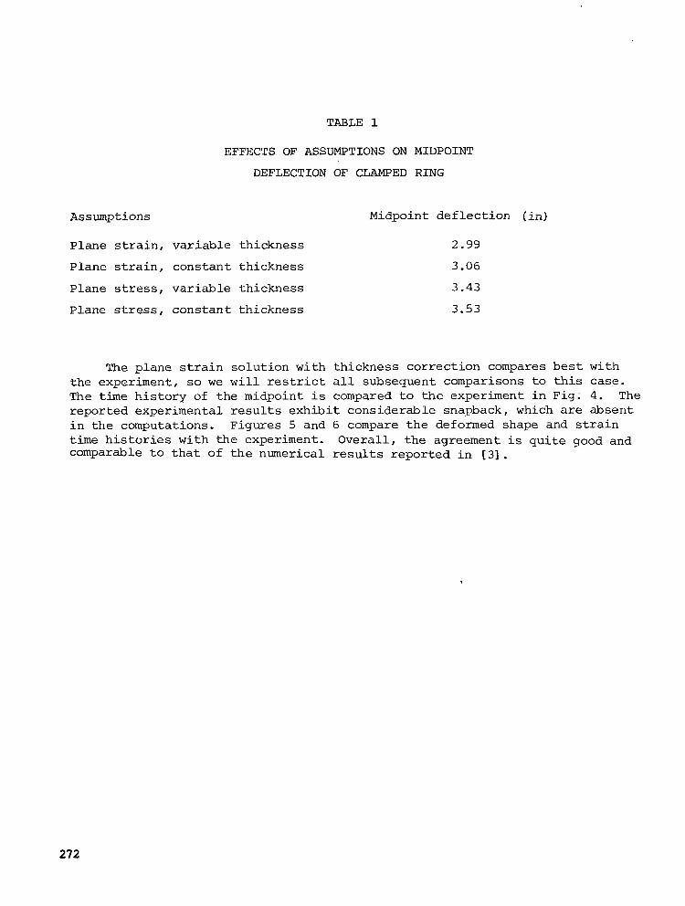
TABLE 1

EFFECTS OF ASSUMPTIONS ON MIDPOINT

DEFLECTION OF CLAMPED R I N G

Assumptions Midpo in t de f l ec t ion ( i n )

P l a n e s t r a i n , v a r i a b l e t h i c k n e s s

P l a n e s t r a i n , c o n s t a n t t h i c k n e s s

Plane stress, va r i ab le t h i ckness

Plane stress, cons t an t t h i ckness

2 -99

3.06

3 -43

3.53

The p lane s t r a in so lu t ion w i th t h i ckness co r rec t ion compares best wi th the experiment , so w e w i l l restrict a l l subsequen t compar i sons t o t h i s case. The time h i s to ry o f t he midpo in t i s compared t o t h e e x p e r i m e n t i n F i g ; 4. The repor ted exper imenta l resu l t s exhib i t cons iderable snapback , which are absen t i n t he computa t ions . F igu res 5 and 6 compare t h e deformed shape and s t r a i n t ime h i s to r i e s w i th t he expe r imen t . Overa l l , t he ag reemen t is q u i t e good and comparable t o t h a t of t h e n u m e r i c a l r e s u l t s r e p o r t e d i n [ 3 ] .

272

I

REFE-NCES

1. K . J . Bathe and H. Ozdemir, "Elastic-Plastic Large Deformation Static and Dynamic Analysis," Computers and S t ruc tu res , V o l . 6, 1976, pp. 81-92.

2. S. Yaghmai and E.P. Popov, "Incremental Analysis of Large Deflections of

3. T. Belytschko and B.J . Hsieh, "Nonlinear Transient Finite Element Analysis with Convected Coordinates," International Journal for Numerical Methods in Engineering, Vol. 7, 1973, pp. 255-271.

4. T. Belytschko and L.W. G l a u m , "Applications of Higher Order Corota t iona l S t re tch Theor ies t o Nonlinear Finite Element Analysis," Computers and Struc- t u r e s , Vol. 10, 1979, pp. 175-182.

5. S.W. Key, "HONDO - A F i n i t e Element Computer Program for the Large Defor- mation Dynamic Response of Axisymmetric Solids," Report SLA-74-QO39, Sandia Laboratories, April 1974.

6. T . J . R . Hughes, and Y.K. Liu, "Nonlinear Finite Element Analysis of She l l s - Par t I , Three Dimensional Shells," to be published Computer Methods i n Applied Mechanics and Engineering.

7. A.E. Green and P.M. Naghdi, "A General Theory of an Elastic-Plastic Contin- uum," Archives of Rational Mechanics and Analysis, Vol. 18, 1965, pp. 251-281.

8. M.L. Wilkins, "Calculation of Elastic-Plastic Flow," Report UCRL-7322- Revision 1, Lawrence Radiat ion Laboratory, Universi ty of Cal i fornia , Livermore, 1969.

9. L. Malvern, Introduction t o t h e Mechanics of a Continuous Medium, Prent ice- H a l l Incorporated, Englewood C l i f f s , New Je r sey , 1969.

10. T. Belytschko, "Nonlinear Analysis - Descript ions and Numerical Stabi l i ty ," i n Shock and Vibration Computer Programs, e d i t e d by W. Pilkey and B. P i lkey , The Shock and Vibration Information Center, 1975, pp. 537-562.

11. H.A. Balmer and E.A. Witmer, "Theoretical-Experimental Correlation of Large Dynamic and Permanent Deformation of Impulsively Loaded Simple Structures ," Report FDL-TDR-64-108, A i r Force Fl ight Dyn. L a b . , Wright-Patterson A i r Force Base, Ohio, 1964.

27 3

Y -

/ DEFORMED

UNDEFORMED

I X

Fig. 1. Deformed and undeformed beam element showing element corotational coorgiGates x,? and local corotational coordinates x,y.

Y I

Fig. 2. Nomenclature for nodal forces and veloci t ies .

I node 1 x , ( r )

27 4

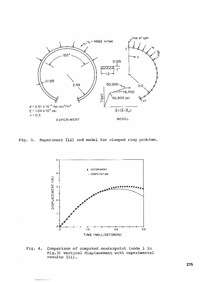
P’ E = Y ’

2.61 X I bs-secz/ in4 1.04 X lo7 psi J!n (!l/l0) 0.3

EXPERIMENT MODEL

Fig. 3. Experiment [ l l ] and model f o r clamped r ing problem.

- 1 X EXPERIMENT

4 t - COMPUTATION

0

TIME (MILLISECONDS)

Fig. 4. Comparison of computed centerpoint (node 1 i n Fig.3) ver t ical d isplacement with experimental results i l l ] .

275

- 3 j : : : : : : : : : : : I 0 i 2 3 4 5 6

X - A X I S

Fig. 5 . Deformed configuration of clamped ring compared t o experimental r e s u l t s [ l l ] .

7, I I I

0 1 2 3 0 2 3 TIME (MILLISECONDS) TIME (MILLISECONDS)

Fig. 6. Comparison of computed strains against experimental resu l t s [ll]; angle i n parenthesis i s for the experimental record.

276

MICROCOMPUTER SYSTEM FOR MEDIUM-SIZED AND EXPERIMENTAL

FINITE ELEMENT ANALYSIS

Yoshiaki Yamada and Hideto Okumura Institute of Industrial Science, University of Tokyo

Tatsumi Sakurai Japan Advanced Numerical Analysis Inc.

SUMMARY

A microcomputer system being developed by the authors is introduced. The parallel effort of compiling a series of compact finite element analysis programs enables the execution of most computation on inexpensive microcomputers. The system is practically maintenance free and can be sustained by individual laboratories of standard scale in the educational or academic environment. AS for the programs, -FEMN is discussed in some detail. The program is an extended version of the original linear analysis program FEM4 and is being tested for application to problems with material nonlinearities.

INTRODUCTION

The finite element analysis has reached the stage where the execution of the structural analysis is often considered routine. This is the case particularly in the industrial environment. However, so far the execution has relied largely on expensive hardware or costly remote time-sharing services. The role of the giant main-frame or super-computer in the solution of large scale problems, e.g. the inelastic analysis of pressure vessels and piping systems operated at elevated temperature, will not be changed even in future applications. But it has been an ambition of engineers to perform a great portion of their analysis jobs on inexpensive and hopefully personal computers and thus be freed from being slave to the large systems. The development of microcomputer and associated finite element analysis programs is a breakthrough in realizing this goal.

The microcomputer system should be stand alone and almost maintenance free so that it can be sustained by individual laboratories especially in the educational or academic environment. The medium-sized engineering problems should be solved within a reasonable time limit and the system could also be adapted to multi-purpose usages, i.e. interactive compilation of fundamental computation routines, data management, preparation of engineering documents and reports, letter writing and so forth. In the present paper a compact system is introduced which is being built by the authors. In a parallel effort, a series of microcomputer finite element analysis

277

programs are being developed. The original version.is FEM4 which is an elastic analysis program of plane stress, plane strain .and axisymmetric problems (ref. 1, 2) . It is extended'to the nonlinear analysis program FEMN by an addition of the restart capability. The results of this innovation are manifold. By an incorporation of user defined subroutine WXLN speci- fying material data, problems with material nonlinearities can be easily handled. Mesh division can be modified in the course of computation and thus the simulation and/or pursuit, for-example, of crack.development in fracture mechanics becomes easier. In the following, some details of the microcomputer system and the program organization of FEMN are described with the example solution of a simple pilot problem.

MICROCOMPUTER SYSTEM STRUCTURE

Figure 1 illustrates the structure of the microcomputer system almost completed at the time, May 1980, of writing this paper. Zilog 280 is used as the 8 bit CPU (Central Processing Unit), and the capacity of main memory, which is composed of a ROM (Read Only Memory) and several RAM (Random Access Memory) boards, totals 64 kilobytes. The transfer of control, address and data between the components of the system is performed exclusively via S-100 bus. For the.purpose of connection and communication a number of interfaces are installed. The 8" floppy disk drive constitutes the secondary memory for mass storage and provides the housing of a compound of operating system, sup- porting language, finite element analysis and other computer programs. The standard disk operating system CP/M is used so that the problems in software exchange can be avoided. At the moment, program languages are BASIC and FORTRAN. It should be noted that two 240K dual disk systems are combined for commanding four floppy disk assemblage, although a dual system kit suffices to perform the standard operation. The authors intend to shorten the overall analysis time by an adoption of parallel processing that uses several CPUs and disk drives. The contemplated inclusion of the hard disk will increase the capacity of secondary memory to a great extent and may open the way to a novel system based on 16 bit microprocessors.

Among the peripherals for 1/0 (Input/Output) purposes shown in figure 1, CRT unit and printer are the essentials. The function of CRT unit is manifold, as it is used for input of the data, interactive operation of the system, cow pilation of program segments and/or,subroutines, temporary display of the computed results, preparation of documents, e.g. the users' manual, and so on. The prepared data, the completed list of the programs and the results of computation can be plugged into the printer for permanent recording. Plotter and graphics terminal are optional, but both are useful for the finite element modeling and post-processing graphics, e.g. automatic mesh generation, model editing and plotting the computed results.

The general purpose programs compiled to date for mounting on the microcomputer system are COMPOL, COMPOS, CALM, FEM4, MICRO-FEM and FEMN. The first two, written in BASIC, are essentially the microcomputer version of 'COMPOsite material computation' being developed by Tsai on a magnetic card calculator (ref.3, 4 ) . In the program names, L and S stand for the laminate

278

. ._ . ..

and sandwich composi te s t ructure respect ively. CALM i s a ma t r ix ope ra t ion program which is b a s i c a l l y a n i n t e r a c t i v e v e r s i o n o f t h e f i r s t group opera- t i o n s i n t h e p r o g r a m CAL ( r e f . 5 , 6 ) . FEM4 and its microcomputer version MICRO-FEM are p r e p a r e d t o s o l v e t h e p l a n e stress, p l a n e s t r a i n and axisymmetric problems and then converted to FEMN to conduc t non l inea r ana lys i s . Restart c a p a b i l i t y is implemented so t h a t t h e i n e l a s t i c material behavior can be handled. Complementary modi f ica t ion i s an add i t ion of t h e u s e r de f ined sub rou t ine MTUN s p e c i f y i n g t h e material propert ies which were for - merly input through e lement data cards . The users who t a i l o r t h e s u b r o u t i n e MTRLN a c c o r d i n g t o t h e i r material d a t a can p e r f o r m c o n v e n i e n t l y t h e - i n e l a s t i c analysis on the microcomputer . An example of MTRLN is shown i n t h e f o l l o w i n g s e c t i o n .

ORGANIZATION OF NONLINEAR ANALYSIS PROGRAM FEMN

FEMN is composed of two p a r t s FEMAB and FEMCD which are concerned with t h e p r e p a r a t i o n o f i n p u t d a t a f i l e and the so lu t ion p rocedure of t h e prob- l e m . The major feature of the program is t h a t i t uses dynamic s t o r a g e a l loca t ion wh ich means the comple te e l imina t ion of common statement . This func t ion is performed by subroutines OPENS, CLOSE, PSEEK and POOLWT as shown i n f i g u r e s 2a and 2b.

The program organization of FEMAB is shown i n f i g u r e 2a. It reads t i t l e a n d c o n t r o l c a r d s f i r s t . Then follows the input of node and element dat'a from which t h e i n d e x o r i n t e g e r j o i n t a r r a y is formed and s t o r e d on IFIL2. IFIL2 accommodates a l s o l o a d d a t a and IFIL6 is e s s e n t i a l l y a s torage of input and processed element data. The formation of strain-displacement matrix16 from t h e d a t a i n I F I L 6 is performed by subroutine MGN and t h e r e s u l t is w r i t t e n on IFIL3 to be read in FEMCD s u b s e q u e n t l y . F i n a l l y t h e i n i t i a l d i s p l a c e m e n t da t a (u sua l ly t he c l ea red ze ro d i sp l acemen t ) are s t o r e d on IFIL5 fo r subse - quent updat ing by the so lu t ion ob ta ined t h rough FEMCD. In t he fo l lowing t he p r i n c i p a l f u n c t i o n s of i n d i v i d u a l s u b r o u t i n e s i n F E W are summarized.

PINPG Preparatory segment for subrout ine INPUTG INPUTG Input genera t ion , read input da ta in sequence and compi le index or in -

RNODE Read node data RELEM Read e lement da ta inc luding material s p e c i f i c a t i o n number and element

MKIDX Make index fo r a t t r i bu t ing merg ing po in t and coord ina te t o i npu t and

t e g e r j o i n t a r r a y

th ickness

processed e lement da ta and a l so create index for skyl ine assemblage of s t i f f n e s s m a t r i x

RLOAD Read loading s tep sequence and nodal force and/or displacement data

OPENS Open s t o r a g e area f o r a r r a y from bottom of POOL i n main memory CLOSE Close a p a r t o r whole s torage area by de le t ing unused a r ray PSEEK Search for a r r a y d a t a by its name POOLWT Debug write w a n t e d a r r a y d a t a i n POOL f o r i n s p e c t i o n

PMGN Prepara tory segment for subrout ine MGN MGN Command sequent ia l genera t ion of e lement matrices ISOBMN Generate e lement s t ra in-nodal displacement matr ix B f o r 3-8 v a r i a b l e

279

node parametr ic element

o f a s s o c i a t e d J a c o b i matrix J

en te r ing d i sp l acemen t da t a o f p reced ing computa t ion fo r restart run

STDMA Evaluate components of strain-nodaldisplacement matrix B and determinant

DISPI I n i t i a l i z e d i s p l a c e m e n t s , by e i t h e r c l e a r i n g f o r i n i t i a l r u n o r

Af t e r t he execu t ion o f FEMAB described above, the next program block FEMCD is c a l l e d by t h e main of FEMN. Functions of FEMCD, whose o rgan iza t ion i s shown i n f i g u r e 2b, are the format ion and assemblage of the e lement s t i f fness matrix and subsequent ly the solut ion of the problem. Material d a t a are inpu t via the . user def ined subrout ine MTRLN and t hen t he s t r e s s - s t r a in matrix D fo r each incrementa l s tage o f loading is e v a l u a t e d i n s u b r o u t i n e D " K N . FEMCD starts i ts operat ion by a t ransfer o r read ing of the da ta s tored on IFIL5, which are t i t l e o f t he p rob lem, i n t ege r da t a , i n i t i a l c l ea red d i sp l acemen t and l oad da t a o r t h e i r v a l u e s o b t a i n e d i n p r e c e d i n g s t e p o f l o a d i n g s e q u e n c e . The stress- nodal displacement matr ix s and e l emen t s t i f fnes s ma t r ix K are formed i n sub- r o u t i n e S " K N , t h e l a t t e r b e i n g s t o r e d i n t h e a p p r o p r i a t e l o c a t i o n s i n t h e o v e r a l l s t i f f n e s s m a t r i x by r e f e r r i n g t o t h e i n d e x p r e p a r e d on IFIL2. IFIL3 and 4 are used as t h e seesaw e x t e r n a l memory fo r i n t ege r da t a and t he e l emen t s t ra in-d isp lacement mat r ix B. S k y l i n e o r p r o f i l e active column method o f da t a a c q u i s i t i o n is used fo r s av ing area i n t h e main memory. Therefore. a l l sub- r o u t i n e s p r e f i x e d by c a p i t a l s SK i n SOLVEN, SKDCNP etc . , take advantage of t he sky l ined fo rm o f s to rage fo r t he man ipu la t ion o f da t a . Newton-Raphson i t e r a t i o n p r o c e d u r e i s i n c o r p o r a t e d i n s u b r o u t i n e SOLVEN, some de ta i l s o f which are d i scussed i n t he nex t s ec t ion conce rned w i th t he so lu t ion o f an e l emen ta ry sample problem. The following summarises the function of individual sub- r o u t i n e s r e l e v a n t t o FEMCD.

PSOLVN Prepara tory segment for subrout ine SOLVEN SOLVEN S o l v e o v e r a l l s t i f f n e s s e q u a t i o n f o r unknown nodal displacement and com-

p u t e r e a c t i o n a t constrained node; i terative procedure i s incorpora ted i n t h i s s o l v e r f o r n o n l i n e a r p r o b l e m s

loading

mat r ix K, s y n t h e s i z e o v e r a l l s t i f f n e s s m a t r i x by r e f e r r i n g t o merging po in t index s tored on IFIL2, and a l so de te rmine equiva len t noda l fo rce f rom cu r ren t stress d a t a f o r e q u i l i b r i u m c h e c k

by s k y l i n e method

VECTWN P r i n t o u t computed d isp lacement and reac t ion vec tor a t each s tage o f

S " K N Evaluate s t ress-nodal displacement matr ix S and e l emen t s t i f fnes s

SWRITE Write components f o r debugging of active columns . in mat r ix S s t o r e d

BWRITE Write components of vector B for debugging SKDCNP Cholesky decomposition of symmetric posit ive definite matrix by sky l ine

SKXMLU Mult iply, add and/or subtract matr ix components in skyl ine s torage CONVCK Check convergence of solution being obtained by Newton-Raphson i terat ive

SKFWD Forward e l imina t ion by s k y l i n e method SKBKW Backward s u b s t i t u t i o n by s k y l i n e method

D " K N Evaluate components of stress-strain matrix D of cons t i t u t ive equa t ion MTRLN User def ined subrout ine spec i fy ing e las t ic a n d i n e l a s t i c material prop-

method

procedure

er t ies

280

STRSUM Add s t r e s s / s t r a i n i n c r e m e n t s t o u p d a t e v a l u e s o f s t r e s s / s t r a i n PRINST Compute p r i n c i p a l stresses a n d t h e i r d i r e c t i o n s STWRN P r i n t o u t s t r e s s / s t r a i n s o l u t i o n s a t r e s p e c t i v e Gauss i n t e g r a t i o n

po in t s , t oge the r w i th coo rd ina te s o f Gauss p o i n t s

F in i t e e l emen t u sed i n FEM4 as w e l l as i n FEMN is 4-8 var iable nodes parametric q u a d r i l a t e r a l w i t h t h e f o l l o w i n g i n t e r p o l a t i o n f u n c t i o n s ( r e f . 7 ) .

For corner nodes 1-4

f o r midedge nodes 5-8

N5 = s5,

N4 = S4 - (N7+N8)/2

N 7 =.S-,, N8 = S8

By c o a l e s c i n g a n e d g e o f t h e q u a d r i l a t e r a l t o a s i n g l e p o i n t a t r i a n g u l a r element i s produced. It can be shown ( r e f .8 , 9) t h a t t h e r e s u l t i n g element coin- c i d e s w i t h t he conven t iona l cons t an t s t r e s s / s t r a in e l emen t when the p r imary quadr i l a t e ra l e l emen t is four-noded. The number of i n t e g r a t i o n p o i n t s i n Gauss quadra ture can be one to f ive by f i v e i n a c c o r d a n c e w i t h t h e u s e r s ' s p e c i f i c a t i o n .

The i n p u t c a r d o r d a t a s e q u e n c e i n FEMN is summarized i n t a b l e I. An example of i npu t da t a p repa ra t ion as w e l l as the u se r de f ined sub rou t ine MTRT.,N i s i l l u s t r a t e d i n t h e n e x t s e c t i o n .

SOLUTION OF SAMPLE NONLINEAR PROBLEM AND REMARKS

AS a sample problem, nonlinear behavior of a composite block specimen shown i n f i g u r e 3 is analysed. The b l o c k c o n s i s t s o f a n i d e a l l y p l a s t i c element 101 and a nonl inear one 501 with a nega t ive s lope segment a t a l a r g e s t r a i n as d e p i c t e d i n f i g u r e 4 based on the material da ta o f f i gu re 3. Loading sequences are summarized i n f i g u r e 3 and t he so l id cu rve . i n f i gu re 4 is t h e theo re t i ca l l oad -d i sp lacemen t r e l a t ion of t h e b l o c k u n d e r a x i a l t e n s i l e l o a d - ing. It is no ted t ha t t he l oad ing cond i t ion i n numer i ca l ana lys i s is given by the fo rce i nc remen t fo r s t ep 1-3 and 7-9, w h i l e i n s t e p 4-6 it is given by t h e displacement increment.

Table I1 is t h e image of i n p u t c a r d s p r e p a r e d f o r t h e s o l u t i o n o f t h e sample p rob lem and s e rves t o i l l u s t r a t e s imp l i c i ty o f the d a t a p r e p a r a t i o n .

2 81

Specifically table I1 is concerned with the first loading sequence, i.e. step 1-3. The solution for consecutive loading conditions, step 4-6 and 7-9 in the present example, is obtained by restarting the execution with the renewal of input data and the use of .the solution obtained in the preceding step and stored on an appropriate file. Table I11 is the subroutine KCRLN written for this sample problem. The program FEMN is versatile because the user can easily tailor the subroutine MTRNL so that it characterizes.particular nonlinear properties of the material of interest. It must be emphasized that the anisotropic material behaviors are easily incorporated in the program.

Figure 5 depicts solution convergence in the sample problem. The iterative procedure that the present version of FEMN employs is a modified Newton- Raphson method with incorporation of equivalent nodal force { Fa). It compensates the imbalance of force equilibrium at the nodes and is given by

J where IF) denotes the prescribed nodal force, [B] and { a ) are the strain-nodal displacement matrix and the current stress. Convergence is satisfactory in the present example and it should be noticed that the computed results lie on the theoretical curve exhibiting sharp turning points.

Test of convergence in case of the large scale problem, sophistication of iterative procedure and extension of the program to three dimensions are the next steps that are to be taken. Moreover, the development of parallel processing and the installation of suitable hard disk will increase the speed and capacity of the system.

REFERENCES

1. Yamada, Y., Hirakawa, T., Nishiguchi, I. and Okumura, H. : Nonlinear Analy- sis by Finite Elements and a Microcomputer System Development, Comp. Appl. in Civil Engng., Nem Chand and Bros, Roorkee, India.

2. FEM4 Users Manual, Nonlinear Analysis Program Research Association, c/o JANA Inc., 1-1-71 Nakamegro, Megro-ku, Tokyo, 153 Japan.

3. Tsai, S.W. and Hahn, H.T.: Introduction to Composite Materials, vol.1, Am-TR-78-201, 1978 Wright-Patterson AFB, Ohio.

4. Tsai, S.W. and Hahn, H.T.: TI-59 Magnetic Card Calculator Solutions to Com- posite Materials Formulas, AFML-TR-4040, 1979, Wright-Patterson AFB, Ohio.

5. Wilson, E.L.: CAL-A Computer Analysis Language for Teaching Structural Analysis, Computers and Structures, v01.10, 1979, pp.127-132.

6. Wilson, E.L.: CAL 78, User Information Manual, Rep. no. UC SESM 79-1, Univ. of California, Berkeley.

7. Bathe, K . J . and Wilson, E.L.: Numerical Methods in Finite Element Analysis, Prentice-Hall, Inc., Englewood Cliffs, 1976.

8. Yamada, Y., Ezawa, Y., Nishiguchi, I. and Okabe, M.: Reconsiderations on Singularity or Crack Tip Elements, Int. J. Num. Meth. Engng., vo1.14, 1979, pp.1525-1544.

9. Yamada, Y.: Matrix Method of Mechanics of Materials, Baifukan, 1980.

282

TABLE I INPUT DATA FORMAT OF FEMN

(1) TITLE CARD (18A4) COL 1-7.2 PROBLEM IDENTIFICATION ETC BY ALPHANUMERIC CHARACTER

(2) CONTROL CARD (2311) COL 1 =O AXISYMMETRIC

=1 PLANE STRAIN =2 PLANE STRESS

2 NUMBER OF INTEGRATION POINTS (1-5) FOR GAUSSIAN QUADRATURE 3* =O INITIAL START

>O RESTART 4- 5* NUMBER OF ITERATION IN NEWTION-WHSON METHOD 6-20 BLANK 21 >O DEBUG WRITE IN MODULE INPUG 22 >O DEBUG WRITE IN MODULE MG 23 >O DEBUG WRITE IN MODULE SOLVEN

(3) NODE HEADER CARD (A4) COL 1-4 ' NODE ' (4) NODE DATA CARDS (A4, 16, 2F10.0, lox, F10.0, lox, 211) COL 1- 4 ' NODE '

7-10 NODE NUMBER 11-20 X (R) COORDINATE 21-30 Y (Z) COORDINATE 41-50 OBLIQUE ANGLE (DEG) OF LOCAL COORDINATE 61 =1 X-DOF CONSTRAINED OR X(R)-DISPL GIVEN

=o OR BLANK FREE OR X(R)-LOATI GIVEN 62 =1 Y-DOF CONSTRAINED OR Y(Z)-DISPL GIVEN

=O OR SLANK FREE OR Y(Z)-LOAD GIVEN

(5) ELEM HEADER CARD (A4) COL 1- 4 ' FLEM' (6) ELEM DATA CARDS (A4, 16, 815, IS*, 215*, F8.0) COL 1- 4 ' ELEM'

7-10 ELEMENT NUMBER 11-15 1ST NODE NO. 16-20 2ND NODE NO. 21-25 3RD NODE NO. 26-30 4TH NODE NO. 31- 35 5TH NODE NO. 36-40 6TH NODE NO. 41-45 7TH NODE NO. 46-50 8TH NODE NO. 51-55* MATERIAL SPECIFICATION NUMBER 56-65* FOR EXTENSION OF PROGRAM BY USERS 66-73 ELEMENT THICKNESS

283

(7) LOAD HEADER CARD (A4) COL 1- 4 'LOAD'

( 8 ) LOAD OR DISPLACEMENT STEP CARD (A4, 16, 6F10.0) * COL 1- 4 ' STEP'

5-10 STEP NUMBER 11-70 FOR PROGRAM EXTENSION

(9) LOAD OR DISPLACEMENT DATA CARD (A4, 16, 2F10.0) COL 1- 4 'LOAD'

5-10 NODE NUMBER ON WHICH GIVEN LOAD OR DISPLACEMENT IS APPLIED 11-20 X(R) GIVEN NODAL FORCE OR DISPLACEMENT 21-30 Y ( Z ) GIVEN NODAL FORCE OR DISPLACEMENT

(10) END CARD (A4) COL 1- 3 'END'

* INDICATES ADDITION OR MODIFICATION APPLIED TO LINEAR ANALYSIS PROGRAM FEM4 AND/OR MICRO-FEM

TABLE I1 INPUT DATA IMAGE OF SAMPLE PROBLEM OF FIGURE 3

2-ELEMENT NONL I NEAR MODEL TEST 22 8 NODE NODE NODE NODE NODE NODE NOflE NODE NODE ELEM ELEM ELEM LOAD STEP LOAD L c m LOAD STEP LOAD L m r I LOAD STEP L c m LOAD LOAD END

2 84

1 1 r-. 13 3 1 1

L A 13 2 0 22 13 2 1 .-I ..-I

C C

C

C

2100

C 3000

3100

C

C EO00

E 2 0 0

C 7000

7200

7 4 0 0 3000

TABLE 111 EXAMPLE OF USER DEFINED SUBROUTINE m R L N

SUBRBUTINE MTRLNIKK, IK, EK, ITER, ISTP:) ........................................................... . I K I 4 1 MFlTERIFlL I D E N T I F I C f l T I B N NUMBER . E K I I K I 9 I 1 CBMPUTED STRf l IN VFlLUE . E K I I K ( I j 1 CBRRESPBNDING STRESS VRLUE . ITER=O, RBUTINE DETERMINES TFINGENT MBDULUS . ITER)O, ITERRTES STRESS FBR COMPUTED STRFIIN VRLUE ........................................................... DIMENSION K K ( 1 1 , I t < ( l ) , E K ( l I M I D = I K I 4 l I K S = I K ( 8 1 I t<9=IK(9 : ) I F ( ITER. GT. 0:) GB TB EO00 :+*-+:% SLBPE OF STRESS-STRRIN CURVE $:+-:+:* IF(MID.GT.01 G 0 TO 3000

Et<(2:)=0. 3 I F ( E K ( I K 9 ) . GT. 1O.OE-35 GB TB 2100 El( ( 1 =2. OE4 GB TO 9000 EK!l)=O.O GB TB 3000

E K ( 2 ) = 0 . 3 I F ( E K I I K 9 ) . GT. 3.OE-3:) GB TB 3100 Et< < 1 ) =2.OE4 GB TB 3000 IF (EKCIK9T . GT. E. OE-3:) GB TB 3200 EN! 1 )=O. 0 GB TO 3000 E K ( l ) = - l . O E + 4 GB TB 3000 *:*:-** STRESS VFILUE F O R CBMPUTED STRRIN *e-:+* IF(MID.GT.0) GB T 0 7000

I F (EK ( I K3:). GT. 10. OE-3:) GB TB E200 E K I I K E ) =2. OE4:+EK (1 K3:) GB TB 9000 EK( IKE1=200 .0 GB TB 3000

IF(EKI IK3: l .GT. 3 .OE-31 GB TB 7200 EK I I KS1=2. DE4*EK ( I K3:) GB Ti3 3000 I F C E K I I K 3 S . GT. 6.OE-35 GB TB 7 4 0 0 EK ( I K I :I =60.0 GB TB 3000 EKI IK8: )=120. O- l .OE4*EK( IK3) RETURN END

**-+*: PERFECTLY PLRSTIC :+*-:+:+

:+*-:+:* NBNL 1 NERR MflTER 1 flL *::+-:+*

*:*:-*:+ PERFECTLY PLRSTIC :+*:-:+:*

**-*:+ NBNL 1 NEnR MRTER 1 R L **:-:+:+

285

PRINTER

@- CRT DISPLAY

HARD DISK GRAPHICS TERMINAL fl "-1 @- FLOPPY DISK DRIVE I MULTI COLOR I

!+ MULTI CPU SYSTEM I

PLOTTER

I I r , I I I I

I I I

6 4 KILOBYTES r-"INTERFACE FOR---, ,""""- """- I

I CPU 2- sI0 I JHARD DISK I GRAPHICS *i

I CPU

-BOARD Z 8 0

88- SI0 FLOPPY ' I

I

'

5-100 BUS (CONTROL.ADDRESS,DATA BUS) 1 I

"" CONTEMPLATED EXTENSION

Figure 1.- Structure of microcomputer system.

2 86

I . . . . .. .

n INPUTG

RNODE

FEMAB

PMGN ~ G N U

I F I L 1 RELEM

MKIDX

I PSEEK I I I STOMA I \\ n

I F I L 5 MAIN

E M C O PSOLVN SOLVEN

I VECTWN

SMXMKN

SWRITE

BWRITE

SKDCNP

I F I L 2

I F I L 3

0 I F I L L

L

CONVCk

SKBKW

DMXMKN MTRLN

STRSUM PRINST

(b) FEMCD.

Figure 2.- Organization of FEMAB and FEMCD.

287

MODULUS HL OF MATERIALS, kgf /mm2 I I I

SPECIFIED LOADING SEQUENCE

TOTAL LOAD DISPLACEMENT INCREMENT I INCREMENT

2 I 1 2 x 1 0 3 I - I I STRAIN RANGE I Hi OF ELEMENT 1 0 1 5 0 1 I I 1 3 I 1 z X 1 o 3 -

7 -12 x103 - 8

- -12 x ~ ~ 3 9

- -12 x103

Figure 3.- Composite block of nonlinear material.

288

0.50 '

0.25 '

0 '

-0.25

-0.50

. -1

-2

Figure 4.- Nonlinear material properties and load-displacement curve.

P.kgf

0.50 -

0.2 5 -

0 -

Q.kgflmm2 2 -

w - E x. -.

Figure 5.- Convergence of solution.

2 89

1. Report No. 2. Government Accession No. 3. Recipient's Catalog No. NASA CP-2147

. "

4. Title and Subtitle 5. Report Date

October 1980 RESEARCH I N NONLINEAR STRUCTURAL AND SOLID MECHANICS 6. Performing Organization Code

7. Authork) 8. Performing Organization Report No. .

Harvey G. McCanb, Jr., and Alnned K. Nmr, &-13990 compilers

10. Work Unit No. 9. Performing Organization Name and Addresr 506-53-53-03

NASA Langley Research Center Hampton, VA 23665

11. Contract or Grant No. I 13. Type of Report and Period Covered

12. Sponsoring Agency Name and Address Conference Paper Na t iona l Aeronau t i c s and Space Admin i s t r a t ion Washington, DC 20546

14. Sponsoring Agency Code

- 15. Sumlementarv Notes

Harvey G. McComb, Jr. : NASA Langley Research Center . Ahmed K. Noor: The George Wash ing ton Un ive r s i ty , Jo in t In s t i t u t e for Advancement

of F l i g h t S c i e n c e s , NASA Langley Research Center .

Most of the pape r s p re sen ted a t t h e symposium are c o n t a i n e d i n N o o r , Ahmed K. ; and McComb, Harvey G., Jr. (eds. ) : Computational Methods in Non l inea r S t ruc tu ra l and So l id Mechan ics . Pe r samon P res s , L td . , 1980 .

16. Abstract

A Symposium on Computa t iona l Methods in Nonl inear S t ruc tura l and Sol id Mechanics was he ld i n Wash ing t ion , D.C., on October 6-8, 1980. NASA Langley Research Center and The George Washington University sponsored the symposium i n c o o p e r a t i o n w i t h the Na t iona l Sc i ence Founda t ion , t he Amer ican Soc ie ty of C i v i l E n g i n e e r s , a n d t h e American Scciety of Mechanical Engineers . The purpose of t h e symposium was to com- municate recent advances and foster i n t e r a c t i o n among r e s e a r c h e r s a n d p r a c t i o n e r s i n s t r u c t u r a l e n g i n e e r i n g , m a t h e m a t i c s ( e s p e c i a l l y n u m e r i c a l a n a l y s i s ) , and corn- pu te r t echno logy . Th i s con fe rence pub l i ca t ion i nc ludes 20 papers; 1 5 were pre- s e n t e d a t research- in-progress sess ions and 5 a t o t h e r s e s s i o n s . The papers d e a l w i t h ( 1 ) n o n l i n e a r a n a l y s i s of b u i l d i n g s t r u c t u r e s ( 2 papers), (2) numer ica l solu- t ion o f nonl inear a lgebra ic equa t ions and Newton ' s method (1 paper), (3 ) non l inea r i n t e r a c t i o n p r o b l e m s ( 2 papers), ( 4 ) s o l u t i o n p r o c e d u r e s for nonl inear p roblems ( 4 p a p e r s ) , (5) c rash dynamics and advanced nonl inear appl ica t ions (3 papers) , (6) material c h a r a c t e r i z a t i o n , c o n t a c t p r o b l e m s , a n d i n e l a s t i c r e s p o n s e ( 5 papers), and (7) formula t ion aspects and special software for n o n l i n e a r a n a l y s i s ( 3 papers).

7. Key Words (Suggested by Author(s))

Nonlinear mechanics S t r u c t u r a l m e c h a n i c s So l id mechan ics

18. Distribution Statement

U n c l a s s i f i e d - Unl imi ted

Computational methods Subject Category 39 9. Security Classif. (of this report) 22. Rice 21. No. of Pages 20. Security Classif. (of this page]

". . -

U n c l a s s i f i e d A1 4 308 U n c l a s s i f i e d

For sale by the National Technical Information Service, Springfield, Virglnla 22161 NASA-Langley, 1980

research in nonlinear structural and solid mechanics - … · tech library kafb, nm nasa conference...

Documents