research journal of business & management · ii editorial board orhan akova, istanbul...
TRANSCRIPT

2148-6689ISSN
PressAcademia publishes journals, books,case studies, conference proceedings andorganizes international conferences.
RJBMResearch Journal ofBusiness & Management
PressAcademia

__________________________________________________________________________________ i
ABOUT THE JOURNAL Research Journal of Business and Management (RJBM) is a scientific, academic, peer-reviewed, quarterly and
open-access online journal. The journal publishes four issues a year. The issuing months are March, June,
September and December. The publication languages of the Journal are English and Turkish. RJBM aims to
provide a research source for all practitioners, policy makers, professionals and researchers working in all
related areas of business, management and organizations. The editor in chief of RJBM invites all manuscripts
that cover theoretical and/or applied researches on topics related to the interest areas of the Journal.
Editor-in-Chief Prof. Suat Teker
Editorial Assistant Melek Tuğçe Şevik
RJBM is currently indexed by
EconLit, EBSCO-Host, Ulrich’s Directiroy, ProQuest, Open J-Gate,
International Scientific Indexing (ISI), Directory of Research Journals Indexing (DRJI), International Society for
Research Activity(ISRA), InfoBaseIndex, Scientific Indexing Services (SIS), Google Scolar, Root Indexing, Journal
Fctor Indexing, TUBITAK-DergiPark, International Institute of Organized Research (I2OR), SOBIAD.
Ethics Policy
RJBM applies the standards of Committee on Publication Ethics (COPE). RJBM is committed to the academic
community ensuring ethics and quality of manuscripts in publications. Plagiarism is strictly forbidden and the
manuscripts found to be plagiarised will not be accepted or if published will be removed from the publication.
Author Guidelines
All manuscripts must use the journal format for submissions.
Visit www.pressacademia.rog/journals/rjbm/guidelines for details.
CALL FOR PAPERS
The next issue of RJBM will be published in June, 2019.
Submit manuscripts to
http://www.pressacademia.org/submit-manuscript/
Web: www.pressacademia.org/journals/rjbm

__________________________________________________________________________________ ii
EDITORIAL BOARD Orhan Akova, Istanbul University, Turkey
Adel Bino, University of Jordan, Jordan Sebnem Burnaz, Istanbul Technical University, Turkey
Isik Cicek, Mediterenean University, Turkey Cigden Aricigil Cilan, Istanbul University, Turkey
Cuney Dirican, Arel University, Turkey Raindra Dissanayake, University of Kelaniya, Sri Lanka
Gabriel Dwomoh, Kumasi Polytechnic, Ghana Ozer Ertuna, Bosphorus University, Turkey
Emel Esen, Yildiz Technical University, Turkey Nadziri Ab Ghani, Universiti Teknologi Mara, Malaysia Syed Reza Jalili, Sharif University of Technology, Iran
Pinar Bayhan Karapinar, Hacettepe University, Turkey Selcuk Kendirli, Gazi University, Turkey
Youngshl Lu, Sun Yat-Sen University, China Michalle McLain, Hampton University, USA
Ghassan Omet, University of Jordan, Jordam Rafisah Mat Radzi, Univiersiti Sains Malaysia, Malaysia
Lihong Song, Shantou University, China Tifanie Turner, Hampton University, USA
Adilya Yamaltdinova, Kyrgyzstan-Turkey Manas University Ugur Yozgat, Marmara University, Turkey
REFEREES FOR THIS ISSUE Pinar Acar, Beykoz University, Turkey
Turkmen Taser Akbas, Pamukkale University, Turkey Senem Besler, Anadolu University, Turkey
Qing-Lan Chen, Xiamen University of Technology, China Steve Dumphy, Indiana University Northwest, USA
Pelin Kanten, Canakkale Onsekiz Mart University, Turkey Malisa Erdilek Karabay, Marmara University, Turkey
Kitsana Manivong, University of Sydney, Australia Michalle McLain, Hampton University, USA
Khaan Na-an, Rajamangala University of Technology Thanyaburi, Thailand Wanchai Panjun, Ramkhamhaeng University, Thailand
Irge Sener, Cankaya University, Turkey Wei-Her Tsai, National Tyaipei University of Nursing and Health Sciences of Taiwan, Taiwan
Mustafa Turhan, Okan University, Turkey

__________________________________________________________________________________ iii
CONTENT
Title and Author/s Page
1. Does organizational justice increase or decrease organizational dissent? Mehtap Ozsahin, Senay Yurur…………………………..…….……………………………………….………………………………………… 1-8 DOI: 10.17261/Pressacademia.2019.1017 RJBM-V.6-ISS.1-2019(1)-p.1-8
2. An empirical examination of the mediating roles of communication and ethical climate Ali Yagmur, Meral Elci…………………….…….………..……………………………………………………………………………………..….. 9-23 DOI: 10.17261/Pressacademia.2019.1018 RJBM-V.6-ISS.1-2019(2)-p.9-23
3. Person owner fit in micro, small and medium companies P. Edi Sumantri, Christantius Dwiatmadja, Ade Banani….……………...……………………………………………………..……. 24-34 DOI: 10.17261/Pressacademia.2019.1019 RJBM-V.6-ISS.1-2019(3)-p.24-34
4. Job stressors and job performance: Modeling of moderating mediation effects of stress mindset Hsiao-Ling Chen, Shih-Chieh Fang………..………..……………………………………………………………………………………..…….. 35-45 DOI: 10.17261/Pressacademia.2019.1020 RJBM-V.6-ISS.1-2019(4)-p.35-45
5. Does patent contribute to stock price in China? Tsui-Min Chen, Chiu-Chi Wei, Hui-Chung Che………..………..………………..…………………………………………………..…….. 46-67 DOI: 10.17261/Pressacademia.2019.1021 RJBM-V.6-ISS.1-2019(5)-p.46-67
6. Is bitcoin becoming an alternative investment option for Turkey? A comparative econometric investigation of the interaction between crypto currencies Mustafa Ozyesil ………………………..………..………………..……………………………………………………………………………..…….. 68-78 DOI: 10.17261/Pressacademia.2019.1022 RJBM-V.6-ISS.1-2019(6)-p.68-78
7. Impact of eight dimensions on the business of specialty coffee shops Chiu-Chi Wei, Chin-Hsin Chiu, Suz-Tsung Wei, Chiou-Shuei Wei……………..……………………….……………………..…... 79-87 DOI: 10.17261/Pressacademia.2019.1023 RJBM-V.6-ISS.1-2019(7)-p.79-87

Research Journal of Business and Management- RJBM (2019), Vol.6(1). p.1-8 Ozsahin, Yurur
_____________________________________________________________________________________ DOI: 10.17261/Pressacademia.2019.1017 1
DOES ORGANIZATIONAL JUSTICE INCREASE OR DECREASE ORGANIZATIONAL DISSENT? DOI: 10.17261/Pressacademia.2019.1017 RJBM- V.6-ISS.1-2019(1)-p.1-8
Mehtap Ozsahin1, Senay Yurur2 1 Yalova University, Department of Management, 77200, Yalova, Turkey. [email protected] , ORCID: 0000-0003-2527-4166 2 Yalova University, Department of Management, 77200, Yalova, Turkey. [email protected] , ORCID: 0000-0002-3859-9827
Date Received: November 29, 2018 Date Accepted: March 10, 2019
To cite this document Ozsahin, M., Yurur, S. (2019). Does organizational justice increase or decrease organizational dissent?. Research Journal of Business and Management (RJBM), V.6(1), p.1-8. Permemant link to this document: http://doi.org/10.17261/Pressacademia.2019.1017 Copyright: Published by PressAcademia and limited licenced re-use rights only.
ABSTRACT Purpose - This study aims to examine the effect of organizational justice on organizational dissent. Methodology- A quantitative research is conducted on white and blue color employees of large scale and medium sized firms operating in automotive industry in Bursa-Turkey. 105 employees, thorough face-to-face survey administration, filled out questionnaire forms. Convenience sampling method is used. Data obtained from those 105 questionnaires were analyzed through the SPSS statistical packet program. Findings - Research findings revealed the positive effects of procedural and distributive justice on upward organizational dissent, whilst the non-significant relation between interactional justice and upward organizational dissent. Analyses results also indicated the non-significant relations of procedural, distributive and interactional justice to latent organizational dissent. Conclusion - The finding of positive effect of procedural justice and distributive justice on dissent behavior, is consistent with the literature, which indicates that justice perceptions of managerial employees increased upward dissent behaviors. However, the finding of this research implying a non-significant effect of interactional justice on organizational justice is inconsistent with the literature, which indicates employees getting better relationship with their managers are more prone to upward dissent. In scope of this survey, employees’ dissent behaviors are influenced by fairness of formal rules and procedures, and acquisitions rather than the fairness of managerial relationships. This distinctive result of this survey may stem from employees’ distrust in relationship with their managers and their prioritization of formal procedures and concrete acquisitions rather than abstract relationships while evaluating the possible retaliations and results of their dissent.
Keywords: Organizational justice, distributive justice, procedural justice, interactional justice, organizational dissent. JEL Codes: M12, M14, M19
1. INTRODUCTION
The questions of “Are employees, who perceive they are treated fair in their organizations, are more prone to opposition or more prone to accept decision and not having need to dissent? Does organizational justice perception affect the organizational dissent? If yes, how does it affect the organizational dissent, does organizational dissent increases organizational justice or not?” has motivated researchers to search the relationship between organizational justice and organizational dissent, so to initiate this study.
Researches on organization justice found out that organizational justice shapes employees’ behaviors which result in positive or negative outputs for organization. Organization citizenship behavior (Lavelle et al., 2009), organizational commitment (Cohen-Charash and Spector, 2001), job satisfaction (Yürür, 2008) and performance (Zapata-Phelan et al., 2009), are considered as some positive outputs of organization justice, while theft (Greenberg, 1990a), retaliation behaviors (Skarlicki and Folger, 1997) and counterproductive behaviors (Fox, et al., 2001) are classified as some negative outputs of organizational injustice.

Research Journal of Business and Management- RJBM (2019), Vol.6(1). p.1-8 Ozsahin, Yurur
_____________________________________________________________________________________ DOI: 10.17261/Pressacademia.2019.1017 2
So, organizational justice perception shaping many attitudes and behaviors of employees, is expected to affect internal dissent in organization. Organization dissent, being defined as expressing disagreement or contradictory opinion in workplace (Kassing, 1998), has been focused on while examining employees’ attitudes and behaviors, as like work engagement (Kassing et al., 2012), whistleblowing (Kassing, 1998), employees’ aggressiveness (Kassing and Avtgis, 1999), employees’ justice perception (Kassing and McDowell, 2008).
Kassing (1997) proposed an organizational dissent model including multistep process: (1) feeling apart from one’s organization (dissent experiment) and expressing disagreement and contradictory opinions about one’s organization (dissent expression) (1998:183). He argues that employees’ dissent expression time and expression way will wary depending organizational, relational and individual influences (1997). Individual influences consist of employees’ personal and demographic characteristics, their attachment to or affinity for their organizations, while relational influences are about the type and nature of relationships employees possess within organizations. Organizational influences also refers to organizational culture, structure and climates which foster or impede dissent (2011:1378-1379). This paper examining the effect of organizational justice on organization dissent will handle organizational justice in the context of the organizational influences.
Moreover, Kassing ve Armstrong (2002) indicated unfair practices in organization as triggers of organizational dissent. Namely, injustice is accepted as an initiative factor that stimulates dissent behavior in organization. However justice is also accepted as enhancer factor that increase organizational dissent in workplace (Kassing ve McDowell, 2008). In other words, organizational dissent behaviors come out of unfair practices and keep going through fair climate in organization. In a fair climate in organization, individual trusts in his/her organization, and prefers to dissent in decision making process without any fear rather than to keep silent. While organizational injustice is an initiative factor of organization dissent in beginning, it becomes undesirable factor subsequently in order organization dissent to be kept on. So, this noteworthy relationship between organizational justice and organizational dissent still needs to be explained in detailed. In this context, this survey, being conducted in Turkey-a developing country having different cultural context and examining the effects of organizational justice dimensions on organizational dissent types in detailed, is expected to fill out a gap and contribute to literature.
In this respect, this study consists of five sections. After a general information about the study is provided in introduction part; the constructs of organizational justice and organizational dissent, and the relationships among those constructs will be explicated in the second section. Detailed information about the survey (such as sample characteristics, measure sources, analyses etc.) and findings of the survey will be submitted in the third and fourth sections of the study respectively. Lastly, the findings will be discussed and the comments about primary results of this survey will be given in the last section.
2. LITERATURE REVIEW
Organizational dissent is defined as employees’ expression of their disagreements and contradictory opinions about workplace policies and practices to various audiences (Kassing, 2011). Based on the type of audience, Kassing (1997, 1998, 2011) classified the organization dissent into three groups. Upward or articulated dissent, in which employees express their disagreements and contradictory opinions in workplace to their directors directly, while in lateral dissent they prefer their co-worker to express their dissent. In both of organization dissent type, audience are internal audience working in organization. However, in third type of organizational dissent, called as displaced dissent, employees can share their contradiction and disagreements about their work place with external audiences as like their family members and friends (Kassing, 1997, 1998, 2011). Indeed Kassing (2000) classified both lateral and displaced dissent into one group, named as latent dissent, because both dissent types include the dissent to the entities (co-workers and family members) who don’t have power to make job related decisions. Thus, actually two types of organizational dissent can be referred: upward (articulated) dissent, to executives who have decision making authority and latent dissent, to any audience who does not have decision making authority. Previously Graham (1986) also classified organizational dissent in terms of content of dissent as personal advantage dissent (eg. dissent about work hours cut or extra duty performing) and principled dissent (eg. dissent about unethical or questionable practices). While Graham’s classification is more related to individual’s moral values, Kassing’s classification concerns with audience, which is mostly affected by individual, relational and organization influences (Kassing, 1997). In this context, organizational justice, as a part of organizational influences, is expected to affect organization dissent types in terms of audience. More understandably, in accordance with perceived organizational justice, employees’ audience preference to express their dissent will change.
Organizational justice literature reveals three types of justice: distributive justice, procedural justice and interactional justice (Masterson et al., 2000). Distributive justice refers to the “employees’ fairness perception about the distribution of outcomes” (Greenberg, 1990), while procedural justice refers to the “perceived fairness of the processes that lead to those outcomes” (Leventhal, 1980). Interactional, the most recently recognized form of justice, refers to the “interpersonal treatment people receive as procedures are enacted”, and is more related to the quality of the relationship between the supervisor and the

Research Journal of Business and Management- RJBM (2019), Vol.6(1). p.1-8 Ozsahin, Yurur
_____________________________________________________________________________________ DOI: 10.17261/Pressacademia.2019.1017 3
subordinate (Bies & Moag, 1986). Greenberg (1993) suggested a four-factor structure for organizational justice by repositioning interactional justice as two separate dimensions- interpersonal and informational. Four-factor view of justice was tested and justified empirically for the first time by Colquitt’s survey in 2001. Informational justice was conceptualized as the fairness of explanations and information provided to the people who are influenced by distribution decisions, while interpersonal justice was defined as fairness of interpersonal treatment provided during the enactment of procedures and distributions of outcomes (Greenberg, 1993).
Scholars investigated positive relation of perceived fairness to job satisfaction (Clay-Warner, Reynolds, & Roman, 2005; Schappe, 1998), organizational citizenship behavior (Moorman, 1991), and organizational trust (Hubbell &Chory-Assad, 2005) of employees. Additionally, perceived fairness affects the way people communicate within organizations and leads them to behave in a cooperative manner (Rahim, Magner, & Shapiro, 2000). As can be seen in literature, increase in perceived organizational justice frequently produces positive outcomes for organization. So, organizational justice, referring to the perceived fairness of employees on organizational procedures, practices and directors in workplace (Folger and Cropanzano, 1998), can be considered as an essential antecedent of employees’ dissent behaviors. Social exchange theory of Blau (1965) constitutes a base to explain this relationship between organizational justice and organizational dissent behavior. According to the theory, individuals have two type of exchange relation to their employers and organizations. One type is economic exchange, in which individual receive some economic outputs in exchange of his/her contribution to organization. The second type is social exchange, in which individual would like to contribute to organization in exchange of her/his social acquisitions. Previous researches demonstrated that organizational justice is an organizational inducement in return employees are willing to contribute to organization (Moorman, 1991; Konovsky ve Pugh, 1994; Masterson, vd., 2000; Rupp ve Cropanzano, 2002; Cropanzano, Prehar ve Chen, 2002; Colquitt, vd. 2012). Kassing and McDowell, (2008) proposed that organizational justice affect employees’ dissent behaviors. Accordingly, employees with high level of justice perception, prefer upward dissent (internal audience, specifically directors to express dissent), which is more beneficial for organization rather than displaced dissent (external audience to express dissent) (Kassing and McDowell, 2008). So, to describe in terms of social exchange terminology, when employee perceives fairness, which can be included in inducements provided by organization, s/he prefers the upward dissent, namely would like to contribute to organization positively.
Some researchers have argued that how fair employees perceive their organizations has a clear impact on how they express dissent (Goodboy, Chory, & Dunleavy, 2009; Kassing & McDowell, 2008). For example, Kassing (2000) indicated that employees who think getting good relationship to their executives are more prone to upward dissent. When employees communicate and express their contradictory opinions to their executives without any hesitation, latent dissent (to co-workers) and displaced dissent (to external entities as like family members) will disappear. Additionally, employees having perception of fairness about decisions and decision making process, will not need latent or displaced dissent resistance to those decisions (Kassing and McDowell, 2008).
Even though previous researches revealed the relationship between organizational justice and organizational dissent empirically (Kassing and McDowell, 2008), how organizational justice types shape the organizational dissent behavior still need to be highlighted. In this context, Goodboy, Chory and Dunleavy (2008), investigated that the distributive and interpersonal justice decreased latent dissent. Same research also indicated a non-significant effect of organizational justice types on upward and displaced dissent (Goodboy et al., 2008). However, literature on employee voice and whistle blowing, which are commonly considered to be synonymous with dissent, has indicated that perceived organizational injustice increased the organizational silent (Pinder and Harlos, 2001; Tangirala ve Ramanujam, 2008; Siefert vd., 2010; Miceli vd., 2012). Namely, injustice in organization discourages employees to speak out. Especially if employees have contradictory options about decisions, in an unfair organization, they prefer to keep on silent with the fear of being injured in future.
In the light of previous researches, it can be argued that organizational justice will increase upward or articulated dissent while decrease latent dissent. As indicated at literature review part, Kassing (2000) proposed two types of organizational dissent upon to types of audience. The expression of dissent to internal audience who have decision making power refers to upward (articulated) dissent, while the expression of dissent to external or internal audience who don’t have decision making authority refers to latent dissent. So displaced dissent to unauthorized-external audience and lateral dissent to unauthorized-internal audience can be embodied in one dimension because both of them are expressed to unauthorized audience, which constitutes the common characteristic of them. Thus, this research focused on upward and latent dissent, on which the effects of distributive, procedural and interactional justice have been searched. So, consisting of three organizational justice dimensions and two dissent dimensions, the following hypotheses are proposed and research model is shaped:

Research Journal of Business and Management- RJBM (2019), Vol.6(1). p.1-8 Ozsahin, Yurur
_____________________________________________________________________________________ DOI: 10.17261/Pressacademia.2019.1017 4
H1a. Procedural justice perception of employees increases the upward dissent.
H1b. Distributive justice perception of employees increases the upward dissent.
H1c. Interactional justice perception of employees increases the upward dissent.
H2a. Procedural justice perception of employees decreases the latent dissent.
H2b. Distributive justice perception of employees decreases the latent dissent.
H2c. Interactional justice perception of employees decreases the latent dissent.
Figure 1: Research Model
3. DATA AND METHODOLOGY
3.1. Sample
The survey is conducted 105 white and blue color employees of large scale and medium sized firms operating in automotive industry in Bursa-Turkey. Questionnaire forms were filled out by employees, thorough face-to-face survey administration. Convenience sampling method is used. Data obtained from those 105 questionnaires were analyzed through the SPSS statistical packet program.
Of the 105 participants, 69 % are male, 31 % female; %57,1 married while %42,9 are single. Most of the participants (63,8 %) are included in 31-40 years-old interval. Employees participating in the survey mostly have higher education level (64,8 % are university graduate; 23 % have post graduate degree) (all sentences 9 punto, calibri, single space)
3.2. Measures
Researchers benefited from the previous scales frequently used in literature to form the measurement instruments of the questionnaire. In this regard, a multidimensional scale of organizational justice based on the measurement instrument of the best known study of Jason A. Colquitt in 2001. The measurement instrument of organizational justice consists of 20 items based on three dimensions – procedural justice (7 items), distributive justice (4 items), interactional justice (9 items). To measure organizational dissent, 15 items-scale adopted from study Kassing (2000) was used. Organizational dissent scale includes two dimension; upward dissent with 8 items and latent dissent with 7 items. Scales used to measure constructs in this study had been translated in to Turkish previously and used at surveys conducted in Turkey (organizational justice scale by Yürür and Demir, 2011; organizational dissent scale by Dağlı, 2015). Overall, 35 items measuring organizational justice and organizational dissent were assessed with five-point-Likert Type scale with anchors 1= strongly disagree and 5=strongly agree.
Cronbach’s alpha values ranging from 0.784 to 0.947 (Cronbach’s α values for Upward dissent with 8 item 0.784; latent dissent with 7 items 0.784; procedural justice with 7 items 0.802; distributive justice with 4 items 0.921; interactional justice with 9 items 0.947) for each constructs indicates reliability of scales.
Distributive Justice
Interactional Justice
Upward Dissent
Latent Dissent
Procedural Justice H1a
H1b
H1c
H2a
H2a
H2a

Research Journal of Business and Management- RJBM (2019), Vol.6(1). p.1-8 Ozsahin, Yurur
_____________________________________________________________________________________ DOI: 10.17261/Pressacademia.2019.1017 5
4. FINDINGS
To test hypotheses, researchers employed multiple regression analyses which incorporates three independent variables-procedural justice, distributive justice, interactional justice-, and two depended variables-latent dissent and upward dissent.
Table 1: Regression Analyses Results
Regression Model
Independent Variable
Depended Variable
Standardized β Sig.
Adjusted R2
F Value
Model Sig.
Model 1
Procedural Justice Upward Dissent
0,327*** 0,001
0,453 29,657 0,000 Distributive Justice 0,478*** 0,000
Interactional Justice 0,053 0,552
Model 2
Procedural Justice
Latent Dissent
-0,040 0,697
0,340 18,898 0,000 Distributive Justice 0,588*** 0,000
Interactional Justice -0,149 0,126
As been depicted on Table 1, findings indicate significant relations of procedural justice (β=0,327; p≤,001) and distributive justice (β=0,478; p<,001) to upward dissent. So H1a and H1b implying that procedural justice and distributive justice respectively increase upward dissent have been accepted. However, H1c stating that interactional justice increase the upward dissent in organization has not been supported (β=0,053; p=,552).
The analysis results for Model 2 also revealed a positive significant relation of distributive justice to latent dissent (β=0,588; p<,001), even though research hypothesis proposed a negative relationship between distributive justice and latent dissent. Moreover, analyses results revealed non-significant relations of procedural and interactional justice to latent dissent (β=-0,040; p=,697 for procedural justice and β=-0,149; p=,126 for interactional justice). So, none of the hypotheses (H2a, H2b, H2c) indicating negative relationships between organizational justice types and latent dissent are supported.
The findings of research analyses are demonstrated below in the research model:
Figure 2: Final Research Model
Supported Not Supported
Distributive Justice
Upward Dissent
Latent Dissent Interactional Justice
Procedural Justice ,327***
,478***
,588*** ,053
-,149
-,040

Research Journal of Business and Management- RJBM (2019), Vol.6(1). p.1-8 Ozsahin, Yurur
_____________________________________________________________________________________ DOI: 10.17261/Pressacademia.2019.1017 6
5. CONCLUSION AND DISCUSSIONS
The main objective of this research is to analyze the effects of organizational justice perceptions of employees on their dissent behavior. In relevant literature, organizational injustice is considered paradoxically as both triggering factor that initiates the dissent (Kassing and Armstrong, 2002) and suppressive factor that impede to evolve the dissent in organization (Kassing and McDowell, 2008). Actually, the relationship between organizational justice and organizational dissent is non-linear. While injustice initiates organizational dissent in organizations, organizational dissent needs justice in order to evolve in organizations. Kassing (1997) argue that some organizational factors, as like structures and practices, define the dissent strategy choices of employees. Organizational justice perception is one of those organizational factors that shapes the employees’ dissent behavior (Kassing and McDowell, 2008; Goodboy, Chory and Dunleavy, 2008). Thus, this survey focused on the effects of organizational justice on organizational dissent behaviors.
One of the findings of this survey was the positive effect of procedural justice and distributive justice on dissent behavior. This finding is parallel to research results of Kassing and McDowell (2008), which indicate that justice perceptions of managerial employees increased upward dissent behaviors. Employees with high level of justice perception believe in that they will not be punished for their expressions, so they are more prone to express their contradictory views about the decisions to their executives without any hesitations in a fair organization. On the other hand, the finding of this research implying a non-significant effect of interactional justice on organizational justice, is inconsistent with Kassing and McDowell (2008)’s research, which indicates employees getting better relationship with their managers are more prone to upward dissent. In scope of this survey, employees’ dissent behaviors are influenced by fairness of formal rules and procedures, and acquisitions rather than the fairness of managerial relationships. This distinctive result of this survey may stem from employees’ distrust in relationship with their managers and their prioritization of formal procedures and concrete acquisitions rather than abstract relationships while evaluating the possible retaliations and results of their dissent. Indeed, this findings is noteworthy for a survey conducted in Turkey, such a high power distance culture country, because most of the surveys conducted in Turkey demonstrated that executives are more influential on employees behaviors and attitudes rather than written rules. Moreover, in a huge number of justice related researches, conducted in Turkey, interactional justice was indicated as the most relevant and influential dimension of organizations justice (Yürür, 2015). This incoherent finding of this research can be caused by sample choice. This survey was conducted on employees working in automotive industry, which corporate companies are operating in. In corporate firms, activities are directed through formal decision making process, rules and procedures rather than managers’ initiatives. So, employees working at such corporate companies are expected to rely on written procedures and rules rather than managerial relations in their attitudes and behaviors, which may constitute an explanation for the distinctive finding of this research.
Another finding of this survey was the positive significant effect of distributive justice on latent dissent, while negative effects of organizational justice on latent dissent are proposed in this research. According to this survey result, the employees’ higher distributive justice perceptions increase their dissent to their co-workers. This positive relationship between distributive justice and latent dissent, which is considered as a mean of resistance to decisions (Kassing and McDowell, 2008), is also striking. When employees perceive outputs of decisions and their acquisitions are fair, their dissent expression to their co-workers increase, which may connote that in a fair climate, employees feel themselves confident and don’t hesitate to dissent. That kind of result oriented behavior can be due to the generation characteristics of employees participating in this survey, most of whom belong to Generation Y. Dissent to co-worker in a fair organizational environment can be Generation Y specific behavior.
Because the survey is conducted on a few automotive firms operating in Bursa distinct, findings cannot be generalized, which constitutes the main binding constraint of this study.
Acknowledgments
This paper was presented at 14th International Strategic Management Conference, which was held between the dates of July 12-14, 2018 in Prague- Czech Republic.

Research Journal of Business and Management- RJBM (2019), Vol.6(1). p.1-8 Ozsahin, Yurur
_____________________________________________________________________________________ DOI: 10.17261/Pressacademia.2019.1017 7
REFERENCES
Bies, R. J., Moag, J. F. (1986). Interactional justice: communication criteria of fairness. In R. J. Lewicki, B. H. Sheppard, & M. H. Bazerman (Eds.), Research on Negotiations in Organizations (Vol. 1, pp. 43-55). Greenwich, CT: JAI Press.
Cohen-Charash, Y., Spector, P. E. (2001). The role of justice in organizations: a meta-analysis. Organizational Behavior and Human Decision Processes, 86, s. 278–321.
Colquitt, J. A. (2001). On the dimensionality of organizational justice: a construct validation of a measure. Journal of Applied Psychology .86(3).pp.386-400
Colquitt, J. A., LePine, J. A., Piccolo, R. F., Zapata, C. P., Rich, B. L. (2012). Explaining the justice–performance relationship: trust as exchange deepener or trust as uncertainty reducer?. Journal of Applied Psychology, 97: s. 1-15.
Cropanzano, R., Prehar, C. A., Chen, P. Y. (2002). Using social exchange theory to distinguish procedural from interactional justice. Group & Organization Management, 27, s. 324 –351.
Dağlı, A. (2015). Örgütsel muhalefet ölçeğinin Türkçe’ye uyarlanması: Geçerlik ve güvenirlik çalışması. Elektronik Sosyal Bilimler Dergisi. 14(53). ss.198-218.
Fox, S., Spector, P. E., Miles, D. (2001). Counterproductive Work Behavior (CWB) in response to job stressors and organizational justice: some mediator and moderator tests for autonomy and emotions. Journal of Vocational Behavior, 59, p. 1–19.
Graham, J. W. (1986). Principled organizational dissent: A theoretical essay. Research in Organizational Behavior, 8, 1-52.
Greenberg, J. (1990a). Employee theft as a reaction to underpayment inequity: the hidden cost of paycuts. Journal of Applied Psychology, 75, p. 561–568.
Greenberg, J. (1990a). Organizational justice: yesterday, today, and tomorrow. Journal of Management, 16, 399-432.
Greenberg, J. (1993). The social side of fairness: interpersonal and informational classes of organizational justice. (içinde), Russell CROPANZANO; Justice in the Workplace: Approaching Fairness in Human Resource Management, Lawrence Erlbaum Associates, Publishers, New Jersey.
Goodboy, A. K., Chory, R. M., Dunleavy, K. N. (2008). Organizational dissent as a function of organizational justice. Communication Research Reports, 25, 255-265.
Kassing, J. W. (1997). Articulating, antagonizing, and displacing: A model of employee dissent. Communication Studies, 48, 311-332.
Kassing, W. (1998). Development and validation of the organizational dissent scale. Management Communication Quarterly, Vol. 12, pp. 183-229
Kassing, J. W. (2000). Investigating the relationship between superior-subordinate relationship quality and employee dissent. Communication Research Reports, 17, 58–70.
Kassing, J. W. (2011). Dissent in organizations. Cambridge, United Kingdom: Polity Press.
Kassing, J. W., Armstrong, T. A. (2002). Someone ‘s going to hear about this: examining the association between dissent –Triggering events and employee’s dissent expressions. Management Communication Quarterly .16(39),pp.39-65
Kassing, J. W., McDowell, Z. (2008). Talk about fairness: Exploring the relationship between procedural justice and employee dissent. Communication Research Reports, 25, 1-10.
Konovsky, M. A., Pugh, S. D. (1994). Citizenship behavior and social exchange. Academy of Management Journal, 37, p. 656–669.
Lavelle, J. J., Brockner, J., Konovsky, M. A., Price, K. H., Henley, A. B., Taneja, A., Vinekar, V. (2009). Commitment, procedural fairness, and organizational citizenship behavior: a Multifoci analysis. Journal of Organizational Behavior, 30, p. 337–357.
Masterson, S. S., Lewis, K., Goldman, B. M., Taylor, M. S. (2000). Integrating justice and social exchange: the differing effects of fair procedures and treatment on work relationships. Academy of Management Journal, 43, p. 738–748.
Miceli, M. P., Near, J. P., Rehg, M. T., Van Scotter, J. R. (2012). Predicting employee reactions to perceived organizational wrongdoing: demoralization, justice, proactive personality and whistleblowing. Human Relations, 65, p. 923–954.
Moorman, R. H. (1991). Relationship between organizational fairness and organizational citizenship behaviors: do fairness perceptions influence employee citizenship?. Journal of Applied Psychology, 76, p. 845–855.
Pinder, C. C., Harlos, H. P. (2001). Employee silence: quiescence and acquiescence as responses to perceived injustice. Research in Personnel and Human Resource Management, 20, 331-69.

Research Journal of Business and Management- RJBM (2019), Vol.6(1). p.1-8 Ozsahin, Yurur
_____________________________________________________________________________________ DOI: 10.17261/Pressacademia.2019.1017 8
Rupp, D. E., Cropanzano, R. (2002). The mediating effects of social exchange relationships in predicting workplace outcomes from Multifoci organizational justice. Organizational Behavior and Human Decision Processes, 89, p. 925-946.
Seifert, D. L., Sweeney, J. T., Joireman, J., Thornton, J. M. (2010). The influence of organizational justice on accountant whistleblowing. Accounting, Organizations and Society 35, p. 707−717.
Skarlicki, D. P., Folger, R. (1997). Retaliation in the workplace: the roles of distributive, procedural, and interactional justice. Journal of Applied Psychology, 82, p. 434–443.
Tangirala, S., Ramanujam, R. (2008). Employee silence on critical work issues: The cross level effects of procedural justice climate. Personal Psychology, 61, pp. 37–68.
Yürür, S. (2008). Örgütsel adalet ile iş tatmini ve çalişanlarin bireysel özellikleri arasindaki ilişkilerin analizine yönelik bir araştirma. SDÜ İktisadi ve İdari Bilimler Fakültesi Dergisi, Cilt 13, Sayı 2, s. 295-312.
Yürür, S. (2015). Türkiye’de örgütsel adalet konusunda yapilan çalişmalara ilişkin bir derleme. (içinde) Edt. Kutanis, Türkiye’de Örgütsel Davranış Çalışmaları-I, Gazi Kitabevi, Ankara.
Zapata - Phelan, C. P., Colquitt, J. A., Scott, B. A., Livingston, B. (2009). Procedural justice, interactional justice, and task performance: the mediating role of intrinsic motivation. Organizational Behavior and Human Decision Processes, 108, p. 93–105.

Research Journal of Business and Management -RJBM (2019), Vol.6(1). p.9-23 Yagmur, Elci
__________________________________________________________________________________ DOI: 10.17261/Pressacademia.2019.1018 9
AN EMPIRICAL EXAMINATION OF THE MEDIATING ROLES OF COMMUNICATION AND ETHICAL CLIMATE DOI: 10.17261/Pressacademia.2019.1018 RJBM- V.6-ISS.1-2019(2)-p.9-23
Ali Yagmur1, Meral Elci2 1 Gebze Technical University, Gebze, Kocaeli, Turkey. [email protected], ORCID: 0000-0003-2839-784X 2 Gebze Technical University, Gebze, Kocaeli, Turkey. [email protected] , ORCID: 0000-0002-0547-0250
Date Received: October 8, 2018 Date Accepted: March 2, 2019
To cite this document Yagmur, A., Elci, M., (2019). An empirical examination of the mediating roles of communication climate and ethical climate. Research Journal of Business and Management (RJBM), V.6(1), p.9-23. Permemant link to this document: http://doi.org/10.17261/Pressacademia.2019.1018 Copyright: Published by PressAcademia and limited licenced re-use rights only.
ABSTRACT Purpose - The aim of this search is to examine the effects of ethical climate and communication climate on the relationship between ethical leadership and employee voice behavior regarding communication perspective. Habermas’ theory of communicative action is mainly used to explain the relationships. Methodology - Survey method is used to test the hypothesized effects in the proposed model. 514 personnel and supervisors from the industries of public services, technology, government, educational services and manufacturing are surveyed. Survey results are analyzed by structural equation modelling. Findings - As a result of the research, all hypothesized relationships in the proposed model are supported revealing that ethical leadership is related to employee voice behavior and this relationship is partially mediated by both communication climate and ethical climate. Conclusion - Working with an ethical leader in an environment perceived as having an effective ethical and communication climate fosters voice of employees, which, in turn, causes to the company to get the benefits of having higher voice of employees.
Keywords: Ethical climate, ethical leadership, communication climate, employee voice, mediator role of communication climate. JEL Codes: M14, M19, D23
1. INTRODUCTION
Significant researches on ethical leadership has already performed (Brown et al., 2005, Walumbwa and Schaubreck 2009, Piccolo et al., 2010; Walumbwa et al., 2011; Avey et al., 2011; Walumbwa et al., 2012; Mayer et. al, 2012). However, communication dimension of ethical leadership which is a part of the definition is generally neglected. Whereas ethical leadership with strong communication climate is obvious to be more effective on the facilities of which ethical leadership provides because definition has already implied the communication dimension. Therefore, this study explores the relationship between ethical constructs and communication constructs empirically. While doing this, it is benefitted from Habermas’ theory of communicative action. In his theory of communicative rationality, Habermas put conditions a rational discussion should meet. “All potential speakers are allowed equal participation in a discourse, everyone is allowed to question any claims or assertions made by anyone, introduce any assertion or claim into the discourse or express their own attitudes, desires, or needs. No one should be prevented by internal or external, overt or covert coercion from exercising the above rights”. In other words, rational argumentation should occur through open debate that is free from the constraints of power and politics. The participants of discourse put forward good, potent reasons for the viewpoints they had so that they can justify their claims by referencing to normative contexts. These are inevitable presuppositions of rational argument (Habermas, 1996). If someone participate an argument without accepting the cited rules above does either behave strategically or commit a performative contradiction (Mingers and Walsham, 2010). On Habermas’s scheme social action is either communicative or strategic. According to Habermas (1984), while strategic action aims to influence the decisions of a rational opponent, the goal of communicative action is to reach consensus. Habermas distinguishes open

Research Journal of Business and Management -RJBM (2019), Vol.6(1). p.9-23 Yagmur, Elci
__________________________________________________________________________________ DOI: 10.17261/Pressacademia.2019.1018 10
and concealed strategic actions. If all participants behave strategically, then they are in open strategic action. If at least one participant believes that all sides are acting communicatively, then they are in concealed strategic action (Baxter, 1987). Communicative action is that “the agents involved are coordinated not through egocentric calculation of success but through acts of reaching understanding” (Habermas, 1984). Communication, according to theory, is about the building of understanding and negotiation about shared activities.
Code of conducts can be obsolete in time and become far away from reflecting the real norm and values (i.e., Trevino and Brown, 2004; Dobson, 2003). In our daily life that uncovered by codes of conducts or rules or ethical programs or that is novel and unexpected ethical issues may occur. We suggest that static code of conducts and ethics programs and static structures and constructs (i.e., rules, ethical approaches, behavioral expectations, etc.) are not enough to prevent detrimental behaviors in a continuously changing world. Dynamic structures are needed to prevent such detrimental behaviors. Communication rationality provides us this dynamism by which only normative thing is the process itself (Benhabib, 1986) changing Kantian individual nature of categorical imperative to collective imperative by rearticulating it to assure the expression of a general will and by providing the rule of argumentation. As can be viewed as a principle of argumentation, Habermas’ moral theory is based on the principle of discourse ethics. If all participants in a discourse approve the claim, then claim becomes valid. In this regard, for instance, committees providing open discourse and guided by a communicative action orientation may account as dynamic structures. In this dynamic structures, voice of any working person can be heard. Ethical leader can play moral agent and moral leader roles. While every participant has equal chance to voice to agree upon and uphold norms and new values, characteristics of moral agent is at the foreground. When a leader or pursuing predefined goals is needed, characteristics of leader is at the foreground. When facilitation is needed for the conditions of communicative action or guidance of participants to reach common understanding, characteristics of moral leader is at the foreground. (Brown et al. (2005) has put forward the moral person and the moral leader concepts for the definition of ethical leadership).
Regarding communicative aspect, the study is analysed whether ethical leadership has an effect on employee voice behavior and whether communication climate and ethical climate mediates this effect. The study begins with a literature review explaining theoretical backgrounds of the hypothesized model. Then, sample, data collection and information about the measures are given. After that, the analyses and results are presented and lastly the findings are discussed and the implications of these findings with limititations and future directions are provided.
2. LITERATURE REVIEW
2.1. Employee Voice
Employee voice includes such actions writing memos, sending e-mails as well as expressing orally. In order to be defined as employee voice, voice should be communicated openly, be pertinent to organization, and be focus on to improve the situation and be received by someone in the organization (Maynes and Podsakoff, 2013).
The concept can be divided as promotive and prohibitive voice behaviors (Bai et al., 2016) as well as supportive, constructive, defensive and destructive voice behaviors (Maynes and Podsakoff, 2013). In this search, we follow LePine and Van Dyne promotive (or constructive) voice behavior definition as a “form of organizational citizenship behavior that involves constructive communication intended to improve the situation” (Van Dyne and LePine, 1998). Employee voice is defined as a form of voluntarily behavior that communicating constructive ideas, comments, suggestions and questions (Van Dyne, Ang and Botero, 2003; Bai et al., 2016). That is, voice specifically focuses on the communication act rather than on other behaviors (Ng and Fedelman, 2012). This construct is specifically selected considering communicative approach.
Another important aspect of definition is discretionary form of the definition. Employees do it not because of force or fear but they want to improve organizational functioning (Van Dyne and Le Pine 1998).
Another important aspect is participation. Employee voice behavior is different from the construct of participation in decision making, because, with voice, employee initiate communications with superiors themselves (Ng and Fedelman, 2012). Thus, we differ employee voice and participation and we see employee voice as an important part of participation and we believe that “without voice there can be no enactment of participation” (Glew, O’Leary-Kelly, Griffin, and van Fleet, 1995).
Employee voice behavior causes improved performance (Wilkinson et al., 2004), makes organizations learns more about their mistakes and weaknesses helping them prevent financial loses (Avey et al., 2012, Detert and Burris, 2007, Grant and Rothbard, 2013). Also, it causes improved motivation, commitment and team working. It facilitates two-way direct communication between management and employees. (Willman et al., 2006). It also causes job satisfaction and less intent to quit (Koyuncu et al., 2013). It plays an essential role in organization success especially during challenging times (Van Dyne and Le Pine, 1998). It has been expressed as a crucial driver of high-quality decisions and success of the organization (Morrison and Milliken, 2000). As well, it is considered to be helpful for the early determination of serious problems (Detert

Research Journal of Business and Management -RJBM (2019), Vol.6(1). p.9-23 Yagmur, Elci
__________________________________________________________________________________ DOI: 10.17261/Pressacademia.2019.1018 11
and Burris, 2007). Increased loyalty and commitment are another beneficial results of enabling voice in workplace (Wilkinson et al., 2018, Farndale et al., 2011).
2.2. Ethical Leadership and Employee Voice
The significant impact of ethical leadership on employee voice behavior has supported by researchers (Brown, et al., 2005; Walumbwa and Schaubroeck, 2009, Avey et al., 2011; Qi and Ming-Xia, 2014; Wang et al., 2015; Wang et al.,2015; Bai et al., 2016; Yuan et al., 2017). Researchers based their empirical findings on social learning process (Walumbwa, Morrison and Christensen, 2012) and social identification process (Zhu et al., 2015). Avey et al. (2012) give another mechanism to explain the relationship, ’social support and structure’. “Ethical leaders tend to listen to employee concerns and be trusted to a greater degree (Brown et al., 2005), thus providing conditions and support for employee to speak up more often”. Walumbwa and Schaubroeck (2009) suggest that, showing high moral standards ethical leaders inspire managers to voice their opinions and suggestions. Zhu et al. (2015) states that ethical leaders, by their behaviors and decisions, inspire employees to demonstrate employee voice behaviors. They found that ethical leadership is positively related to voice behavior. De Hoogh and Den Hartog (2008) states that ethical leaders facilitates employee voice behavior by encouraging employees to express their opinions and by being eager to listen their concerns. If employees believe that they are provided with a fair and highly moral environment, they are more likely to speak up like their leader as they learn (Brown et al. 2005).
Wang et al. (2015) states that literature explains the relationship by 4 basic statements. First, ethical leaders, by taking into consideration of employees’ thoughts and feelings, are perceived as a person who is interested in employees’ opinions, consequently, they encourage employees to voice suggestions. (Brown et al., 2005; Avey, et al., 2012). Second, establishing appropriate employee conduct and emphasizing the importance of ethical behavior, leaders become role models for employees and encourages them to give voice (Walumbwa and Schaubroeck, 2009; Avey, et al., 2012; Walumbwa, et al., 2012). Third, with open and truthful interaction with employees, ethical leaders build interpersonal trust between employees and them, thereby causing more voice up (Brown et al., 2005; Walumbwa and Schaubroeck, 2009). Fourth, proclaiming the importance of voice and strengthening voice legitimacy and improving the environment by which employee voice can foster, ethical leaders provide a climate in which employees feel that voicing their opinions is both safe and meaningful (Avey, et al., 2012 ; Klaas, Olson-Buchanan, and Ward, 2012 ).
Regarding communicative action; leaders will try to provide right conditions for communicative rationality and they guide the argumentation toward reaching understanding. While engaging such an act, they can “draw on different forms of participative decision-making” (Patzer et al., 2018). As we already outlined, decision-making is strongly related with employee voice. Thus we expect that ethical leadership has relationship with employee voice and we propose the following hypothesis:
H1: Ethical leadership is positively related to employee voice behavior.
2.3. Ethical Leadership and Ethical Climate
Ethical climate is defined by Victor and Cullen (1988) as “shared perceptions of what correct behavior is and how ethical issues will be dealt with” and by Schneider (1975) as “stable, psychologically meaningful, shared perceptions employees hold concerning ethical procedures and policies existing in their organizations”. The concept of ethical climate is shaped by external factors which can affect the perceptions of employees.
Mulki et al. (2009) uses “Path-Goal Theory” to explain the relationship between ethical leadership and ethical climate. Alike, Mayer et al. (2010) use social learning theory of Bandura (1977, 1986) to explain the relationship. While exploring the role of ethical leadership on ethical climate, Groejan et al. (2004) uses the concept of ‘values’. Schminke et al. (2005) also uses the concept of ‘values’ reporting that Trevino et al. (2000) discussed the importance of a leader’s character for ethical leadership and stating that ‘values’ “are the glue that holds things together and they must be conveyed from the top of the organization”. Explaining the relationship, Schminke et al. (2005) bases their theoretical approach on the various factors like role modeling, rewards, selection and communication.
Signaling to employees the existence of formal procedures and perceptions and showing the correct behaviors which are expected, encouraged and valued and following procedures and perceptions and implementing reward and punishment systems, ethical leaders will probably be the cause of which employees get stronger ethical climate perception in organizations. Therefore we propose the following hypothesis:
H2: Ethical leadership is positively related to ethical climate.
2.4. Ethical Leadership and Communication Climate
Ethical leadership definition has inherently includes communication. On the other hand, communication climate is related to communication satisfaction within organization. And “employees tend to think of climate when they respond to general

Research Journal of Business and Management -RJBM (2019), Vol.6(1). p.9-23 Yagmur, Elci
__________________________________________________________________________________ DOI: 10.17261/Pressacademia.2019.1018 12
questions about communication” (Downs and Hazen, 1977) meaning that communication climate is evidence of communication. Therefore, communication climate should be in relation with any construct regarding communication.
Another explanation is about moral leader and moral agent role of ethical leaders (Trevino et al., 2006) and communicative rationality process. According to Habermas (1996)’ communicative rationality process, the basic conditions for an ideal discourse entails that “all affected parties could participate in the discourse” and that “there should be a power-free medium for all participants”. The role of ethical leader under the circumstances is moral agent which provides the necessitate conditions for the discourse and facilitates the discourse for shared base of norms and values. But, despite the qualifications, Habermas classifies power as control or steering medium (Baxter, 1987), so there should be a moral leader to prevent the use of power which can be used to manipulate discourse conditions. Moreover, according to communicative rationality process depending on the situations and their intentions, participants can “switch between strategic and communicative action” (Habermas, 1984). There should be a moral leader to prevent such a switch.
Another explanation to influence of ethical leadership on communication climate is based on Patzer et al. (2018)’ approach. According to their approaches, Habermas points out the difference between two main domains of modern social life, the “life-world” and the “system-world”. Lifeworld is the back ground of ordinary life, mainly private, relatively prejudiced, moderately guileless and essential to our satisfaction as human beings. System-world is composed of formal structures, such as governments, corporations. Individuals in system world have official roles and defined goals and they seek to realize these goals (Levine, 2017). In the lifeworld, the aim of interaction is mainly communicative while in systems world it is mainly strategic. (Patzer Voetglin, 2018). So there should be a person who makes the balance between these two worlds. Ethical leadership gives the definition of moral leader ad moral agent. While moral leader handles system-world by behaving like a leader in classical definition and by role modelling for the others to pursue organizational predefined goals, moral agent tries to communicate with followers in the lifeworld to reach ideal communication medium by expressing communicative behavior. Therefore we propose the following hypothesis:
H3: Ethical Leadership is positively related to communication climate.
2.5. Communication Climate and Employee Voice Behavior
Communication climate can be defined as the mood of relationships between people who work or live together and includes only communicative elements of a work environment (Guzley, 1992).
Participation is one construct to use to explain the relationship. One of important dimensions related with communication climate is perceived participation in decision making (feeling of having a voice in decision). Communication climate consist of participative decision making (Redding, 1972) and as already stated, without voice there can be no enactment of participation (Glew et al., 1995). Consequently, an interaction is inevitable.
Trust is another construct to use to explain the relationship. Trust is the glue of the relationship between communication climate and employee voice behavior. For avoiding distrust, communication climate is needed (Appelbaum et al, 2000); as a type of extra- role behavior (Van Dyne and LePine, 1998), employee voice entails mutual trust. Thus we put forward that positive communication climate increase employee voice and that hypothesis:
H4: Communication climate is positively related to employee voice behavior.
2.6. Ethical Climate and Employee Voice Behavior
The relationship between ethical climate and employee voice behavior has already been proven by researchers (Victor and Cullen, 1988; Trevino and Youngblood, 1990; Gaertner, 1992; Weber, 1992, 1993; Wimbush, 1993; Cohen, 1993a; Newman, 1993; Trevino and McCabe, 1994; Paine, 1994; Wimbush and Shepherd, 1994). This relationship is also empirically proved by Wang and Zhao (2016) while in their studies they explore the relationship between ethical climate and organization silence. Drawing on team-level social learning perspective, Bai et al. (2016) proved that ethical leadership will foster ethical climate causing employee voice behaviors. Furthermore, Gok et al. (2018) support that ethical climate affects employee voice behavior positively.
Employee voice behavior is a voluntary act. It has discretionary nature. Because of this, employee’s voice is “largely depend upon whether the surrounding environment is in favor of speaking up” (Bai et. al., 2016). On the other hand ethical climate encourages employees to act and make decisions (Wang and Hsieh, 2013). So an interaction is inevitable. Another explanation may depend on trust. Providing highly moral standards ethical climate supports trust and we already outlined before employee voice entails mutual trust. Therefore we propose the following hypothesis:
H5: Ethical climate is positively related to employee voice behavior.

Research Journal of Business and Management -RJBM (2019), Vol.6(1). p.9-23 Yagmur, Elci
__________________________________________________________________________________ DOI: 10.17261/Pressacademia.2019.1018 13
Ethical Leadership
Ethical Climate
Communication Climate
Employee Voice
H3
H2 H5
H4
H1
2.7. Mediating Roles of Ethical Climate and Communication Climate
Mayer et al. (2010), suggest that “the mediating role of climates is implicit in the early conceptualization of organizational climate” referring to studies of Litwin and Stringer (1968), Campbell et al. (1970), Schneider (1983) and Hofmann and Stetzer (1998); Schminke et al. (2005); Zohar and Luria (2005) which examines the relationship between organizational climates with relevant outcomes Thus, mediator role of communication and ethical climate is expected. So we propose the following hypothesis:
H6: Communication climate and ethical climate mediates the relationship between ethical leadership and employee voice behavior.
Our research model is depicted below as Figure 1.
Figure 1: Research Model
3. DATA AND METHODOLOGY
3.1. Participants and Procedure
Data were collected from the employees of various organizations placed in Istanbul, Kocaeli, and Ankara between November 2016 and June 2018. Industry types include public services, technology, government, educational services and manufacturing. Total number of responded questionnaires is 514. All participants were guaranteed anonymity during this process in the study. We introduced a time lag in our survey to maximize consistency. We gave detailed information taken to ensure the confidentiality of our respondents.
3.2. Measures
All items were measured on a five point Likert-type scale where 1 = strongly disagree and 5 = strongly agree. Ethical leadership was measured using the 10-item ELS scale developed by Brown et al. (2005). Questions of original scale can be found at Appendix A.
Ethical climate was measured using the 7-item ethical climate scale developed by Schwepker et al. (1997) inspired by the scale developed by Qualls and Puto (1989). Questions of original scale can be found at Appendix A.
Communication climate was measured using the 5-item communication climate sub-dimension of communication satisfaction questionnaire developed by Downs and Hazen (1977). Questions of original scale can be found at Appendix A.
Employee voice was measured using the 6-item ethical climate scale developed by Van Dyne and Le Pine (1998). Questions of original scale can be found at Appendix A.
SPSS 21 and IBM SPSS AMOS 21 for Windows programs are used to perform all analyses.
3.3.Exploratory Factor Analysis
The varimax rotation technique is applied and explained with 4 factors in this research. These factors are named ethical leadership, communication climate, ethical climate, and employee voice. Variables which has factor loading higher than 0.5 were extracted. Eigenvalue greater than 1 (EVG1) component retention criteria is used to determine the number of factors (Iacobucci and Churchill 2010). That one factor was extracted from the six employee voice items is disclosed by factor

Research Journal of Business and Management -RJBM (2019), Vol.6(1). p.9-23 Yagmur, Elci
__________________________________________________________________________________ DOI: 10.17261/Pressacademia.2019.1018 14
analysis (see Table 1). 73.35 % of total variance is accounted by factor analysis. Internal consistency is generally measured with cronbach alpha. The results showed that the Cronbach Alpha value for each dimension was above 0.8 representing satisfactory consistency of the items (see Table 4). The results also showed that the KMO and Bartlett`s test of sampling adequacy was significant for each variable were sufficiently (KMO=.965).
Table 1: Exploratory Factor Analysis Results
Ethical Leadership Ethical Climate Comm. Climate
Employee Voice
EthL5 0,788
EthL3 0,777
EthL8 0,765
EthL9 0,757
EthL7 0,749
EthL6 0,743
EthL10 0,721
EthL4 0,7
EthL1 0,685
EthL2 0,672
EthC2
0,8
EthC4
0,783
EthC3
0,781
EthC1
0,755
EthC5
0,736
EthC6
0,66
EthC7
0,613
CSQ-C3
0,813
CSQ-C2
0,756
CSQ-C1
0,694
CSQ-C4
0,668
CSQ-C5
0,633
EmpV5
0,802
EmpV3
0,799
EmpV1
0,769
EmpV6
0,756
EmpV4
0,703
Extraction Method: Principal Component Analysis. Rotation Method: Varimax with Kaiser Normalization.
a Rotation converged in 7 iterations.
Code and Questions of original scales can be found at Appendix A.
Research Journal of Business and Management -RJBM (2019), Vol.6(1). p.9-23 Yagmur, Elci
__________________________________________________________________________________ DOI: 10.17261/Pressacademia.2019.1018 15
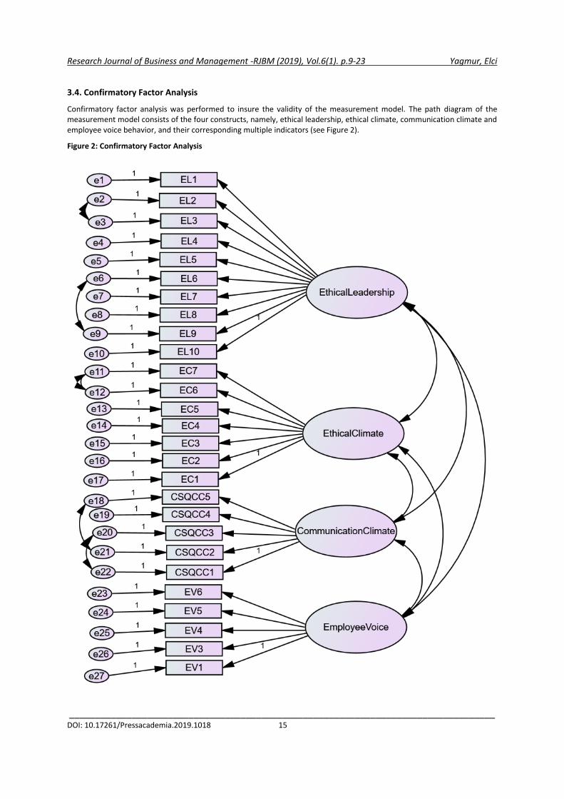
3.4. Confirmatory Factor Analysis
Confirmatory factor analysis was performed to insure the validity of the measurement model. The path diagram of the measurement model consists of the four constructs, namely, ethical leadership, ethical climate, communication climate and employee voice behavior, and their corresponding multiple indicators (see Figure 2).
Figure 2: Confirmatory Factor Analysis

Research Journal of Business and Management -RJBM (2019), Vol.6(1). p.9-23 Yagmur, Elci
__________________________________________________________________________________ DOI: 10.17261/Pressacademia.2019.1018 16
Multiple fit indexes were used to assess the fit of the model. Specifically, chi-square statistic (χ2), comparative fit index (CFI), incremental index of fit (IFI), goodness of fit index (GFI), normed fit index (NFI), and Tucker–Lewis index (TLI) were used. The model showed good fit with CFI = 0.948, IFI = 0.948, GFI=0.877, TLI = 0.942, NFI=0.926, RSMEA = 0.064 and χ2(195) = 978.831 (see Table 2)
Table 2: Model Fit Indexes
Indicator Name Reference Measurement
Model Simplified Model (For Mediation Analysis)
χ2 – 978.831 258.013
χ2/df <5 Bentler (1990) 3.127 2.966
p value >0.05 Wheaton et al. (1977) 0.00 0.00
CFI >0.9 Bentler (1990) 0.952 0.975
GFI >0.9 Schumacker and Lomax (2010) >0,8 Doll et al.,1994; Green et al., 2012
0.887 0.938
TLI >0.9 Klem (2000) 0.942 0.970
NFI >0.9 Bentler and Bonett (1980) 0.928 0.963
RMSEA <0.08 Byrne (2010); Hair et al.(2010) 0.064 0.062
The validity of measurement model is accessed through convergent and discriminant validity. Convergent validity is assessed by means of standard factor loading, the average variance extracted (AVE) and composite reliability (CR) (Fornell and Lacker, 1981, Hair et al., 2006). The standardized factor loading indicates the association between the variables. Standard factor loadings should be over 0.50 (Fornell and Lacker, 1981, Hair et al., 2006). Average variance extracted (AVE) shows the average amount of variance in indicator variables that a construct is managed to explain. Average variance extracted should be over 0.50 (Fornell and Lacker, 1981, Hair et al., 2006). Composite Reliability is the measure for internal consistency of reliability that does not assume equal indicator loadings on the contrary of cronbach alpha. Composite reliability should be over 0.60 (Hair et al., 2006).
Standard factor loadings are above 0.50, the AVE values are above 0.50 and CR (Composite Reliability) values are above 0.60 (See Table 3 and 4)
Table 3: Composite Reliability (CR), Average Variance Extracted (AVE) and Maximum Shared Variance (MSV) and Correlations between Constructs
CR AVE MSV Employee
Voice Ethical
Leadership Comm. Climate Ethical Climate
Employee Voice 0,905 0,656 0,503 0,810 Ethical Leadership 0,958 0,715 0,671 0,709 0,846
Comm Climate 0,852 0,538 0,355 0,596 0,646 0,761
Ethical Climate 0,952 0,738 0,671 0,683 0,819 0,556 0,859
Table 4: Validity, Reliability and Internal Consistency
Construct
Estimate Cronbach α AVE CR
Ethical Leadership EthL1 0,841 0.962 0.715 0.958
EthL2 0,81
EthL3 0,843
EthL4 0,787
EthL5 0,862
EthL6 0,888
EthL7 0,87
EthL8 0,884
EthL9 0,817
EthL10 0,863

Research Journal of Business and Management -RJBM (2019), Vol.6(1). p.9-23 Yagmur, Elci
__________________________________________________________________________________ DOI: 10.17261/Pressacademia.2019.1018 17
Construct
Estimate Cronbach α AVE CR
Communication Climate CSQCC1 ,760 0,845 0,538 0,852
CSQCC2 ,743
CSQCC3 ,811
CSQCC4 ,772
CSQCC5 ,826
Ethical Climate EthC1 ,877 0.953 0.738 0.952
EthC2 ,889
EthC3 ,925
EthC4 ,877
EthC5 ,856
EthC6 ,798
EthC7 ,784
Employee Voice EmpV1 ,830 0.904 0.656 0.905
EmpV3 ,794
EmpV4 ,772
EmpV5 ,844
EmpV6 ,748
The discriminant validity determines whether the constructs in the model are highly correlated among them or not. In this study, discriminate validity is assessed by comparing the average value extracted (AVE) with the squared correlation between each pair of factors (Fornell and Lacker, 1981) (see Table 3). Another indicator, maximum shared variance can be used to determine discriminant validity (Byrne, 2013) by comparing MSV value with AVE (MSV < AVE). Our model support this criteria, too (see Table 3).
3.5 Hypotheses Testing
After performing exploratory and confirmatory factor analyses and confirming the fit of the measurement model, the hypothesized relationships are examined. Figure 3 shows the standardized values.
Table 2 shows the model fit indexes and Table 5 shows regression weights. According to these results,
Ethical leadership is positively related to employee voice (standardized β=0.32, CR=4.39), therefore, H1 was supported.
Ethical leadership is positively related to ethical climate (standardized β =0.82, CR=20.60), therefore, H2 was supported.
Ethical leadership is positively related to communication climate (standardized β =0.65, CR=12.09), therefore, H3 was supported.
Ethical climate is positively related to employee voice (standardized β =0.29, CR=4.59), therefore, H4 was supported.
Communication climate is positively related to employee voice (standardized β =0.23, CR=4.55), therefore, H5 was supported.

Research Journal of Business and Management -RJBM (2019), Vol.6(1). p.9-23 Yagmur, Elci
__________________________________________________________________________________ DOI: 10.17261/Pressacademia.2019.1018 18
Figure 3: Proposed Model’s Path Diagram
Table 5: Regression Weights
Path Estimates β SE CR p
Stand. Non stand.
Ethical_Climate<---Ethical_Leadership ,820 ,879 ,043 20,600 ***
Communication_Climate<---Ethical_Leadership ,654 ,385 ,032 12,089 ***
Employee_Voice<---Ethical_Climate ,294 ,273 ,060 4,586 ***
Employee_Voice<---Communication_Climate ,229 ,388 ,085 4,555 ***
Employee_Voice<---Ethical_Leadership ,319 ,318 ,072 4,391 ***
In order to examine the mediation effect, further analysis was performed. A direct path between ethical leadership and employee voice behavior was drawn (Figure 4). The model showed a good fit with χ²/df=2.966, GFI=0.938, AGFI=0.914, CFI=0,975, RMSEA=0.062 (see Table 2). A significant positive direct effect of ethical leadership on employee voice behavior existed (Standardized β value is 0.71). We compared beta values of the model (β= 0.71) with proposed structural model (β=0.32). A partial mediating effect exists if the relationship between independent variable (ethical leadership) and dependent variable (employee voice behavior) is reduced in magnitude and becomes less significant (Baron and Kenny,

Research Journal of Business and Management -RJBM (2019), Vol.6(1). p.9-23 Yagmur, Elci
__________________________________________________________________________________ DOI: 10.17261/Pressacademia.2019.1018 19
1986). Therefore, ethical climate and communication climate together partially mediates the relationship between ethical leadership and employee voice behavior.
Figure 4: Path Diagram For Mediation Analysis
Table 6 shows the path analyses results. According to these results
Direct effect of ethical leadership on employee voice behavior is significant and positive (β = 0.32)
Direct effect of ethical leadership on ethical climate is significant and positive (β = 0.88)
Direct effect of ethical climate on employee voice behavior is significant and positive (β = 0.27). Indirect effect for this path is (0.88*0.27 = 0.24).
Direct effect of ethical leadership on communication climate is significant and positive (β = 0.39)
Direct effect of communication climate on employee voice behavior is significant and positive (β = 0.39). Indirect effect for this path is (0.39*0.39 = 0.15).
Total indirect effect of between ethical leadership and employee behavior is 0.39 (0.24+0.15), providing evidence of ethical climate and communication climate’s mediating effect.
Table 6: Path Analysis Results
Path Total effect Direct effect Indirect effect
Ethical leadership→Ethical climate 0.879*** 0.879*** –
Ethical leadership→Communication climate 0.385*** 0.385*** –
Ethical leadership→Employee voice behavior 0.71*** 0.32*** 0,39***
Ethical climate→Employee voice behavior 0.273*** 0.273*** –
Comm. climate→Employee voice behavior 0.388*** 0.388*** – *** is significant at the 0.01 level (2-tailed).
4. FINDINGS AND DISCUSSIONS
Our research examined the relationship between ethical leadership and employee voice behaviors in line with the communication perspective and sought to examine the mediation effects of ethical climate and communication climate on this relationship. Consistent with our hypotheses we found that ethical leadership is positively related to employee voice behavior and communication climate and ethical climate mediates the relationship between ethical leadership and employee voice behavior.
Considering the benefits of having employee voice and ethical leadership and creating strong communicative continuum, organizations may seek to train the supervisors to cultivate strong ethical perspective and culture. This yields effective ethical mechanisms in which employees know how to respond ethical issues. In this way, the institutionalization of ethics by

Research Journal of Business and Management -RJBM (2019), Vol.6(1). p.9-23 Yagmur, Elci
__________________________________________________________________________________ DOI: 10.17261/Pressacademia.2019.1018 20
building ethical boards/committees and making ethics as daily routine will improve ethical perception resulting with increase of the prestige and the performance of the company. Researches reveal that more customers prefer to work with the companies which have ethical concern.
4.1. Limitations and Future Directions
This research has several limitations. Firstly, our sample is composed of individual members of the organizations as the respondents who rated online all the questions by themselves. Instead survey can be carried out face to face to reduce the questionnaire errors or the misunderstandings.
Having cross sectional data is another limitation. Longitudinal designs can draw stronger inferences regarding causality. A future work could benefit from this.
Another limitation is that there was no private sector or public services discrimination. A future work may consider this kind of discrimination or a similar study can be performed on non-profit organizations.
Unmeasured variables is another limitation. There could be other mechanisms influencing the relationship between ethical leadership and employee voice or the effect of ethical leadership on other constructs. Future search should continue to explore these relationships.
Although this study found strong support for the hypotheses proposed, a weakness is the use of one-dimensional ethical climate and one-dimensional ethical leadership constructs. Future researchers are encouraged to use multi-dimensional ethical leadership and ethical climate constructs. Future researchers may also expand the constructs used here in order to get complete picture.
A future research may examine the ideal communication medium construct with preparing appropriate scale. This construct may give ideal communication medium definition and measure the idealness of medium. Individual and organizational performance of economic systems world as well as individual and organizational communicative abilities can be measured by this construct. Construct can be inter disciplinary.
A future research may examine the effect of existing and operating ethical board/committee. In this regard, whether the existence of ethical board/committee has an effect of unethical behaviors can also be measured. Moreover, operating effectiveness of ethical board/committee is measured by regarding the relationship with ethical leadership and unethical behavior.
Consequently, although the importance of ethical climate and ethical leadership concepts is revealed, organizations do not give the deserved credits for them. Theoretical and empirical academic studies will continue to play a critical role to remind them the importance of these concepts.
4.2. Implications
We found that perceptions of strong communication climate and ethical climates were associated with higher voice of employees causing to improved performance (Wilkinson et al., 2004), prevent financial and social losses (Avey et al., 2012, Detert and Burris, 2007, Grant and Rothbard, 2013) and improve the quality and innovation of the company’s services and products (Morrison and Milliken, 2000). This also implies that the ethical climate and communication climate in an organization is subject to at least some degree of control. Thus, if proactive steps are taken to enhance the ethical or communication climate, this may increase the effect of ethical leadership creating trustworthy organization causing the benefits of this.
Our results confirm that ethical leadership has an important role to yield employee voice behavior. Therefore, ethical leadership may be considered a model guiding managers. Ethical programs and ethical training should be considered to foster ethical leadership acts. The issues dealt with the questions of ethical leadership scale can help managers shape their behaviors.
Our search emphasizes that high ethical working environment is beneficial to organizations. Managers need to help in creating an environment where the ethics supported.
Our results illustrate that providing open communication channels and interactions enhance employee voice behaviors. Employees feel more motivated when they are encouraged to voice up. Participation to the decisions make them feel as a part of organization. For this to happen, managers need to provide enough time to spend with them, organization needs to provide enough resources to maximize participation so that the employees would be able to show improved performance and help prevent financial and social losses.

Research Journal of Business and Management -RJBM (2019), Vol.6(1). p.9-23 Yagmur, Elci
__________________________________________________________________________________ DOI: 10.17261/Pressacademia.2019.1018 21
5. CONCLUSION
Habermas’ world is in flux and change. This is similar to changeability of ethical contexts and instability of ethical issues, there are always novel ones. The only way to handle them, dynamic structures should be built up. In this way one could be able to find a solution. Considering an example ethical committees could be a good candidate. In these committees, managers listen and discuss shared norms, values, novel issues, alternatives and if needed, they decide as part of the role of moral leader. Committees can be kept alive to reflect daily problems and all employee participation should be provided at least representation level. After reaching consensus or understanding, all the employees are informed with the results. Our search suggest to strengthen ethical structures not by focusing to create static structure like code of conducts but by focusing the development with continuous discourse.
REFERENCES
Avey, J. B., Wensing, T. S., Palanski, M. E. (2012). Exploring the process of ethical leadership: The mediating role of employee voice and psyhological ownership. J Business Ethics (2012), 107:21-34.
Bai, Y., Lin, L., Liu, J.T. (2017). Leveraging the employee voice: a multi-level social learning perspective of ethical leadership. The International Journal of Human Resource Management, DOI: 10.1080/09585192.2017.1308414.
Bandura, A. (1977). Self-efficacy: Toward a unifying theory of behavioral change. Psychological Review, 84,191–215.
Bandura, A. (1986). Social foundations of thought & action. (Prentice-Hall, Englewood Cliffs).
Bojuwon, M., Bojuwon, Y. B. (2015). Measuring lecturers commitment scales: A second order confirmatory factor analysis (CFA). International Journal of Education and Research, Vol. 3 No. 3 March 2015.
Brown, M. E., Trevino, L. K. (2006). Ethical leadership: A review and future directions. The Leadership Quarterly, 17, 595–616.
Brown, M. E., Trevino, L. K. (2006). Ethical leadership: A review and future directions. The Leadership Quarterly, 17, 595–616.
Brown, M. E., Trevino, L. K., Harrison, D. A. (2005). Ethical leadership: A social learning perspective for construct development and testing. Organizational Behavior and Human Decision Processes, 97, 117–134.
Brown, M. E., Trevino, L. K., Harrison, D. A. (2005). Ethical leadership: A social learning perspective for construct development and testing. Organizational Behavior and Human Decision Processes, 97, 117–134.
Cullen, J. B., Victor, B., Stephens, C. (1987). An ethical weather report: Assessing the organization's ethical climate. Organizational Dynamics, 50—62.
Downs, C. W., Hazen, M. D. (1977). A factor analytic study of communication satisfaction. The Journal of Business Communication, 14 (3): 63-74.
Elçi, M., Alpkan, L. (2009). The impact of perceived organizational ethical climate on work satisfaction. Journal of Business Ethics 84, 297–311.
Fairtlough, G. H. (1991). Habermas’ Concept of “Lifeworld”. Systems Practice, Vol. 4, No. 6, 1991.
Glew, D. J., O’Leary-Kelly, A. M., Griffin, R. W., van Fleet, D. D. (1995). Participation in organizations: A preview of the issues and proposed framework for future analysis. Journal of Management, 21(3), 395–421.10.1177/014920639502100302[Crossref], [Web of Science ®], [Google Scholar], p. 402).
Grojean, M., Resick, C., Dickson, M., Smith, D. B. (2004). Leaders, values, and organizational climate: examining leadership strategies for establishing an organizational climate regarding ethics. Journal of Business Ethics 55, 223–241.
Habermas, J. (1984). Theory of communicative action. Volume 1: Reason and the rationalization of society. Boston: Beacon Press.
Habermas, J. (1987). Theory of communicative action. Volume 2: Lifeworld and system a critique of functionalist reason. Boston: Beacon Press.
Habermas, J. (1996). Moral consciousness and communicative action. Cambridge: MIT Press.
Habermas, J. (1998). Between facts and norms: Contributions to a discourse theory of law and democracy. Cambridge, UK: Polity Press.
Mayer, D. M., Kuenzi, M., Greenbaum, R. L. (2010). Examining the Link between ethical leadership and employee misconduct: The mediating role of ethical climate. Journal of Business Ethics, 95:7-16.
Mulki, J. P., Jaramillo, J. F., Locander, W. B. (2009). Critical role of leadership on ethical climate and salesperson behaviors. 86, 125-141.
Ng, T. W. H., Feldman, D. C. (2012). Employee voice behavior: A meta-analytic test of the conservation of resources framework. Journal of Organizational Behavior, 33, 216-234.

Research Journal of Business and Management -RJBM (2019), Vol.6(1). p.9-23 Yagmur, Elci
__________________________________________________________________________________ DOI: 10.17261/Pressacademia.2019.1018 22
Park, J. Y., Nawakitphaitoon, K. (2018). The cross‐cultural study of LMX and individual employee voice: The moderating role of conflict avoidance. Hum Resour Manag J. 2018; 28: 14–30.
Schminke, M., Ambrose, M. L., Neubaum, D. O. (2005). The effect of leader moral development on ethical climate and employee attitudes. Organizational Behavior and Human Decision Processes 97, 135–151.
Schwepker, C. H. Jr., Ferrell, O. C., Ingram, T. N. (1997). The influence of ethical climate on role stress in the sales force. Journal of the Academy of Marketing Science, 25 (Spring): 99–108.
Trevino, L. K., Brown, M. E. (2004). Managing to be ethical: Debunking five business ethics myths. Academy of Management Executive, 2004, Vol.18, No. 2.
Van Dyne, L., LePine, J. A. (1998). Helping and voice extra-role behaviors: evidence of construct and predictive validity. Academy of Management Journal, Volume 14, 108-119.
Walumbwa, F. O., Schaubroeck, J. (2009). Leader personality traits and employee voice behavior: Mediating roles of ethical leadership and work group psychological safety. Journal of Applied Psychology, 2009, Vol. 94, No. 5, 1275–1286.
Wang, X., Zhao, X. (2016). Experimental study of organizational ethical climate and silence: Based on the theory of psyhological expectations. 2016 2nd Asia-Pacific Management and Engineering Conference.
Wang, D., Gan, C., Wu, C., Wang, D. (2015). Ethical leadership and employee voice: employee self-efficacy and self-impact as mediators. Psychological Reports: Employment Psychology & Marketing 2015, 116, 3, 751-767. © Psychological Reports 2015.
Wang, D., Gan, C., Wu, C., Wang, D. (2015). Ethical leadership and employee voice: Employee self-efficacy and self-impact as mediators. Psychological Reports: Employment Psychology & Marketing 2015, 116, 3, 751-767.
Yang, Q., Liu, M. X. (2014). Ethical leadership, organizational identification and employee voice: examining moderated mediation process in the Chinese insurance industry. Asia Pacific Business Review, 20:2, 231-248, DOI: 10.1080/13602381.2013.823712.
Yuan, L., Vu, M. C., Nguyen, T. T. N. (2017). Linking ethical leadership to employee voice behavior: The role of leader-member exchange. International Journal of Management & Business Studies, Vol.7, Issue 3, July-Sept 2017.
Zhu, W., He, H., Trevino L. K., Chao, M. M., Wang, W. (2015). Ethical leadership and follower voice and performance: The role of follower identifications and entity morality belief. The Leadership Quarterly 26 (2015) 702-718.

Research Journal of Business and Management -RJBM (2019), Vol.6(1). p.9-23 Yagmur, Elci
__________________________________________________________________________________ DOI: 10.17261/Pressacademia.2019.1018 23
APPENDIX A : SCALES
Ethical Leadership (Brown et al. (2005))
EthL1 – My supervisor listens to what employees have to say
EthL2 - My supervisor disciplines employees who violate ethical standards
EthL3 - My supervisor conducts his/her personal life in an ethical manner
EthL4 - My supervisor has the best interests of employees in mind
EthL5 - My supervisor makes fair and balanced decisions
EthL6 - My supervisor can be trusted
EthL7 - My supervisor discusses business ethics or values with employees
EthL8 - My supervisor sets an example of how to do things the right way in terms of ethics
EthL9 - My supervisor defines success not just by results but also the way that they are obtained
EthL10 - When making decisions, My supervisor asks “what is the right thing to do?”
Ethical Climate (Schwepker et al. (1997))
EthC1 - My company has a formal, written code of ethics
EthC2 - My company strictly enforces a code of ethics
EthC3 - My company has policies with regards to ethical behavior
EthC4 - My company strictly enforces policies regarding ethical behavior
EthC5 - Top management in my company has let it be known in no uncertain terms that ethical behaviors will not be tolerated
EthC6 - If a sales executive in my company is discovered to have engaged in unethical behavior that results primarily in personal gain (rather than corporate gain), she or he will be promptly reprimanded
EthC7 - If a sales executive in my company is discovered to have engaged in unethical behavior that results in primarily corporate gain (rather than personal gain), she or he will be promptly reprimanded
Communication Climate (Downs and Hazen (1977))
CSQ-C1 - Company communication motivates and stimulates an enthusiasm for meeting its goals
CSQ-C2 - The people in my organization have great ability as communicators
CSQ-C3 - The company's communication makes me identify with it or feel a vital part of it
CSQ-C4 - I receive on time the information needed to do my job
CSQ-C5 - Conflicts are handled appropriately through proper communication channels
Employee Voice (Van Dyne and Le Pine (1998))
EmpV1 - I develop and makes recommendations concerning issues that affect this work group.
EmpV2 - I speaks up and encourages others in this group to get involved in issues that affect the group.
EmpV3 - I communicate my opinions about work issues to others in this group even if my opinion is different and others in the group disagree with me.
EmpV4 - I keep well informed about issues where my opinion might be useful to this work group.
EmpV5 - I get involved in issues that affect the quality of work life here in this group
EmpV6 - I speak up in this group with ideas for new projects or changes in procedures.

Research Journal of Business and Management -RJBM (2019), Vol.6(1). p.24-34 Sumantri, Dwiatmadja, Banani
_____________________________________________________________________________________ DOI: 10.17261/Pressacademia.2019.1019 24
PERSON OWNER FIT IN MICRO, SMALL AND MEDIUM COMPANIES DOI: 10.17261/Pressacademia.2019.1019 RJBM- V.6-ISS.1-2019(3)-p.24-34 P. Edi Sumantri1, Christantius Dwiatmadja2, Ade Banani3 1 Jenderal Soedirman University, Doctoral Program in Management Science Faculty of Economics and Business, Purwokerto, Indonesia. [email protected], ORCID: 0000-0002-1289-9725 2 Satyawacana Christian University, Department of Economics and Business, Salatiga, Indonesia. [email protected], ORCID: 0000-0002-8849-7562 3 Jenderal Soedirman University, Department of Economics and Business, Purwokerto, Indonesia. [email protected] ORCID: 0000-0002-9899-8598
Date Received: December 27, 2018 Date Accepted: March 4, 2019
To cite this document Sumantri, P. E., Dwiatmadja, C., Banani, A. (2019). Person owner fit in micro, small and medium companies. Research Journal of Business and Management (RJBM), V.6(1), p.24-34. Permemant link to this document: http://doi.org/10.17261/Pressacademia.2019.1019 Copyright: Published by PressAcademia and limited licenced re-use rights only.
ABSTRACT Purpose - The main purpose of this study is to examine whether the Person Owner Fit as a dimension developed in the theory of Person Environment Fit has a significant influence on job satisfaction and intention to leave. Methodology - In this study we tested a sample of employees working in the micro, small and medium business sector in Banyumas district, Central Java, Indonesia, as many as 225 respondents, using structural equation modelling (SEM). Findings - The test results show p-value of 0.011 <0.05 (cut of value), with its CR value of 2.542> 2.00 and p-value of 0.102> 0.05 (cut of value), with its CR value amounting to 1,634 <2,00 Conclusion - There is a positive and significant effect of the dimension of Person Owner Fit (P_Own_Fit) on job satisfaction, and there is no significant effect of the Person Owner Fit (P_Own_Fit) dimension on the intention to leave.
Keywords: Person–owner fit, person–job fit, job satisfaction, intention to leave. JEL Codes: K31, K41, J41
1. INTRODUCTION
Conformity, match, and harmony are important factors that must be considered by various parties to achieve the same goal. In organizations it can be done through consideration of various aspects that involve employee values and values that exist within the organization. The theory used in examining conformity aspects refers to person-environment (PE) fit theory (Caplan, 1983; French, 1974), who assume that individuals prefer an environment having similar characteristics to themselves (Kroeger, 1995). PE-Fit is compatibility that occurs when there is a match between the characteristics of an individual and his/her working environment (Kristof‐Brown, Zimmerman, & Johnson, 2005). In assessing conformity aspects, researchers generally try to compare the internal aspects of an individual (for example, values, personality, goals, abilities) with elements from the external environment (for example, values, culture, climate, goals, and demands) as ways to understand and predict employee attitudes and behaviour. Behaviour is considered as a function of the interaction between people and situational factors (Cable & Judge, 1996; Chatman, 1989; Schneider, 1987).
The theory of Person-Environment Fit (PE-Fit) has developed measurements of aspects of conformity, match, harmony between individuals and their environment, so that this theory is considered to be able to construct concepts used in measuring various types of "fit" or conformity, which encourage the concept to develop into a construct multidimensional fit (Kristof-Brown & Guay, 2011). This is in accordance with the concept stated by Harrison (2007) who assesses compatibility or suitability by

Research Journal of Business and Management -RJBM (2019), Vol.6(1). p.24-34 Sumantri, Dwiatmadja, Banani
_____________________________________________________________________________________ DOI: 10.17261/Pressacademia.2019.1019 25
combining one or more attributes that focus on individuals and their environment (J. R. Edwards, 2008; Harrison, 2007). Multidimensional constructs of conformity at various levels that have been developed by researchers to date include: Person–Vocation fit (PV Fit), Person–Job Fit (PJ Fit), Person–Organization Fit (PO Fit), Person-Team Fit atau Person–Group Fit (PG Fit), Person–Individual Fit (PI Fit).
Person-Vocation Fit refers to the suitability taking place between the work environment and the expertise and interests of individuals towards work that leads to vocational related to one's career path (Holland, 1997; Moos, 1987; Parsons, 1909; Super, 1953). Person-Job Fit (P-J Fit) is the suitability of individuals with their jobs (J. R. Edwards, 1991). At the organizational level, Person-Organization Fit is used to assess aspects of conformity between individuals and the organizations in which they work (Kristof-Brown, 1996), this suitability encourages employees to do their job according to the characteristics and values that exist within the organization. At the group level the dimensions of Person-group fit, or person-team fit are often used to consider conformity or match that focuses on individuals with their coworkers and work teams (Kristof-Brown & Stevens, 2001; Kristof‐Brown, Barrick, & Kay Stevens, 2005; Werbel & Gilliland, 1999). Conformity at the individual level has developed the Person-Individual Fit dimension that describes the suitability of individuals with other individuals in explaining reciprocal relationships in their work environment.
The Person-Individual Fit dimension assesses similarity, match, harmony, in various aspects such as personality whose results show that personality similarities are associated with more quality exchanges between leaders and followers (Ashkanasy & O'connor, 1997; Bauer & Green, 1996; Engle & Lord, 1997; Graen & Cashman, 1975; Liden, Wayne, & Stilwell, 1993; Phillips & Bedeian, 1994; Steiner & Dobbins, 1989), thus improving better interpersonal relationships, higher performance, facilitating communication, increasing effectiveness in interaction (Engle & Lord, 1997; Meglino, Ravlin, & Adkins, 1991; Miles, 1964), increase the amount of communication between individuals (Engle & Lord, 1997; Lincoln & Miller, 1979; Miles, 1964), social integration in organizations (O'Reilly, Caldwell, & Barnett, 1989), and reduce conflict and role ambiguity (Tsui & O'reilly, 1989; Turban & Jones, 1988). Perspectives that explore dimensions of conformity in the domain of Person Supervisors Fit (PS-Fit) tend to assess the compatibility between leaders and subordinates through various aspects considered such as values (Hoffman, Bynum, Piccolo, & Sutton, 2011; Vianen, 2000), personality (Schaubroeck & Lam, 2002), work style (Turban & Jones, 1988), lifestyle (Dimarco, 1975), and leadership style (Chuang, Judge, & Liaw, 2012).
The PE-Fit research is mostly applied to medium and large scale organizations whose organizational structure is well established and managed by management without direct involvement from the owner. However, PE Fit research has not been applied to smaller scale organizations such as micro, small and medium enterprises (MSMEs) which are often characterized by the owner's active involvement in managing his business. In general, small business owners want to have control over their environment (Cardon & Stevens, 2004; Jack, Hyman, & Osborne, 2006) and ensure that employees will share the same values and beliefs (Williamson, 1981) . This illustrates the situation of MSMEs, which generally show owner dominance and are actively involved in managing their business. Communication between the owner as a leader and their employees can lead to harmonious relationships in a family atmosphere (Matlay, 1999), and flexible work practices are factors that support the success of small businesses (Walker & Brown, 2004). Thus, the compatibility between employees and owners is an important factor that needs to be explored further to support the success of MSMEs.
The dimensions of Person-Individual Fit (PI Fit) to date have explored the relationship between individuals and their colleagues (Antonioni & Park, 2001), job applicants with recruiters (Graves & Powell, 1995), mentor to protege (Turban & Dougherty, 1994), leaders with subordinates (Adkins, Russell, & Werbel, 1994; Kristof‐Brown, Zimmerman, et al., 2005; Vianen, 2000), followers and leaders (Colbert, 2004; Krishnan, 2002), similarity of superior personality with subordinates (Schaubroeck & Lam, 2002), suitability of manager's goals with employees (Witt, 1998). However, researches related to the PE-Fit field are hardly to find. There has not been found a match between the employee and the business owner (Owner) who also acts as the leader of the company, so researchers assume this concept needs to be developed by expanding the dimensions in the Person Environment Fit theory so that this theory can be applied more flexibly to organizations in all business scales.
The Person Environment Fit theory which includes multidimensional conformity can only be used to measure conformity in large and well-established organizations, but the theory cannot be applied to organizations with micro and small scale businesses because they are still managed by the owner. Therefore, it is necessary to add a dimension of conformity that can be applied to micro and small businesses so that the theory of Person Environment Fit can be applied in all business scales, these dimensions are named as the Person Owner Fit dimension.

Research Journal of Business and Management -RJBM (2019), Vol.6(1). p.24-34 Sumantri, Dwiatmadja, Banani
_____________________________________________________________________________________ DOI: 10.17261/Pressacademia.2019.1019 26
2. LITERATURE REVIEW
2.1. MSMEs in Indonesia
The number of business actors in Indonesia is still dominated by MSMEs having a considerable contribution in creating jobs, acting as a place to earn income and develop skills. (Sartika & Soedjoedono, 2002). MSMEs are called as sectors having labour intensive not capital intensive (BI, 2011), it means more empowering the workforce to obtain optimal results, so that human resource management must be applied appropriately in order to be able to grow and develop better.
In this study, the definition of MSMEs refers to the Indonesian Central Bureau of Statistics (BPS), using reference based on the quantity of labour, with the criteria for micro businesses having a workforce of 1 - 4 people, small businesses having a workforce of 5 to 19 people and medium-sized businesses having workers 20 to 99 people ("Badan Pusat Statistik, Kabupaten Banyumas," 2017).
2.2. Person Owner Fit (P Own Fit)
This dimension was developed based on the theory of social exchange which became the root of the development of psychological contracts. Social Exchange Theory shows that rational personal interests encourage social interaction of society and personality are the main driving factors of human behaviour in the organization (House, Shane, & Herold, 1996). This means that individuals in relationships with others will try to maximize the benefits they get (Blau, 1964; Homans, 1958). The concepts that develop in psychological contracts are grouped into transactional contracts and relational contracts. The contract emphasizes "a belief system that an individual and his/her employer will hold an exchange agreement between them" (Dabos & Rousseau, 2004).
Transactional contracts are more directed at economic motives and short-term work agreements, while relational contracts focus more on affective involvement and personality development on the job and expect long-term employment relationships (Millward & Brewerton, 1999). High involvement and attachment in relational psychological contracts, is characterized by the similarity of views in relationships made between employers and workers (Filotheos Ntalianis, 2015). The long-term, proactive and dedicated actions of employees will create a climate full of trust, and at the same time become a key component of psychological relationships (Montes & Irving, 2008). Relational contracts are said to have a positive relationship with psychological ownership (Aggarwal & Bhargava, 2010), this is associated with long-term security which creates a feeling of attachment to the organization. This feeling is characterized by the individual's perception of ownership of an object both material and immaterial that can manifest itself (Belk, 1988; Dittmar, 1992; James, 1890). Thus, the suitability between employees and owners will build psychological ownership in employees so that it is assumed that the Person Owner Fit has a negative correlation with the desires or intentions of employees leaving the organization or company.
Hypothesis 1: The Person Owner Fit has a negative and significant influence on the desires or intentions of employees leaving the organization
The Person Owner Fit dimension also refers to the ASA (Attraction, Selection, and Attrition) framework model that illustrates that organizational goals are stated implicitly or explicitly by the founder in the hope of generating policies, special practices and their combination to develop organizations with structural, process and cultural characteristics special. The ASA framework model will determine the characteristics of people who are interested, chosen by, and who remain in the organization (Schneider, Goldstiein, & Smith, 1995). Individual interest in a particular organization is initially based on implicit estimates of the suitability of individual characteristics with the attributes inherent in potential work organizations. The next stage refers to formal and informal selection procedures used by organizations in recruiting and hiring people according to the attributes desired by the organization. The final stage emphasizes the process of friction so that people will leave organizations they don't like. Thus, the ASA framework model will form an environment that results in homogeneity because the same people will live in different organizations and will leave (Schneider et al., 1995), this leads to the existence of suitability between employees and the owner.
To differentiate between the dimensions of Person Owner Fit (P-Own-Fit) and the dimensions of Person Individual Fit (PI Fit), the basis of Stewardship theory is used to describe situations when executives as stewards / servants are motivated to act according to principals' wishes, they will not leave the organization and try reaching the target organization (Donaldson & Davis, 1991). This theory emphasizes the existence of aspects relating to the owner, while the PI Fit dimension developed in the PE-Fit theory has not shown involvement directly from the owner of the organization or company. Conformity or matching of views between owners and employees is one aspect that needs to be developed in micro, small and medium enterprises, because business owners generally still rely on their employees not only to carry out their assigned tasks, but also ready to use their initiatives in working outside which has been narrowly defined in the job description (Gatewood & Feild, 1987). Thus the Person
Research Journal of Business and Management -RJBM (2019), Vol.6(1). p.24-34 Sumantri, Dwiatmadja, Banani
_____________________________________________________________________________________ DOI: 10.17261/Pressacademia.2019.1019 27
Owner Fit (P-Own-Fit) can be seen as a dimension that needs to be considered in assessing the suitability between employees and business owners as well as supporting multidimensional developments in the Person-Environment Fit theory, and it is assumed that the Person Owner Fit has a positive correlation with satisfaction employee work.
Hypothesis 2: Person Owner Fit has a positive and significant influence on employee job satisfaction
2.3. Person Job Fit (PJ-Fit)
This dimension refers to the suitability of a person's characteristics with the characteristics of his work. Experts define Person-Job Fit (P-J Fit) as a match between a person's ability to the demands of his work (i.e., demands-abilities) or someone's desires with his work attributes (needs-supplies) (J. R. Edwards, 1991; Kristof-Brown, 1996). Demands-abilities (DA) include aspects related to KSA (knowledge, skills and abilities) and personality, while needs-supplies fit includes aspects related to the interests and characteristics of work (Chuang, Shen, & Judge, 2016). Complementarity-based perspective (Muchinsky & Monahan, 1987) in relation to DA Fit, it states that one can complete the characteristics of his environment when there is a match of one's ability to the requirements of the job with the content of DA Fit, namely "KSAO" (Knowledge, Skill, Ability, and Other characteristics) (Kristof‐Brown, 2000; Rynes & Gerhart, 1993).
Experience in work can be a determining factor in assessing P-J Fit, in addition to the possibility that requires work that must be held by individuals who have certain personality types to obtain better performance (Rynes & Gerhart, 1993). Personality characteristics and skills / expertise related to work are considered to be important factors to assess perceptions of complementary compatibility (Piasentin & Chapman, 2007), this is in line with research that emphasizes personality aspects in measuring perceptions of conformity with work (Lauver & Kristof-Brown, 2001). In considering aspects of meeting needs, individuals will compare their own needs with regard to recognition and social involvement with those provided by the environment (French & Kahn, 1962). So, the suitability of interests will support positive results such as satisfaction, retention, and achievement, in accordance with empirical evidence that shows that the P-J Fit is related to job performance / work (Li & Hung, 2010; Wang, Zhan, McCune, & Truxillo, 2011), job satisfaction (Cable & DeRue, 2002; Wang et al., 2011), turnover / turnover intentions (Wang et al., 2011), turnover / turnover decisions (Cable & DeRue, 2002), and OCB (Organizational Citizenship Behaviours) (Li & Hung, 2010), so that hypotheses 3 and 4 are developed as follows:
Hypothesis 3: Person Job Fit has a positive and significant influence on employee job satisfaction.
Hypothesis 4: Person Job Fit has a negative and significant influence on employee's intention to leave the organization.
2.4. Job Satisfaction
A pleasant or positive emotional state that results from an assessment of one's work or work experience (Locke, 1976), and other opinions state that cognitive and / or affective evaluations of one's work are more or less positive or negative (Brief & Weiss, 2002). Job satisfaction has the potential to influence various behaviours in the organization and contribute to the level of employee welfare (George; & Jones, 2012), so that employee job satisfaction is an important indicator for the organization. Employee satisfaction or dissatisfaction has implications for employee performance, organizational commitment, organizational citizenship behaviour, intention to move or turn over, and work attitude. Job satisfaction is positively correlated with employee performance and with organizational commitment (George; & Jones, 2012; Judge & Larsen, 2001). Employees who are satisfied with their jobs tend to perform better than those who are not satisfied. Job dissatisfaction, on the other hand, has been linked to absenteeism, delay, turn over, and other negative attitudes (Randolph & Johnson, 2005). Job satisfaction is also explained by various types of P-E fit (Spanjol, Tam, & Tam, 2015; Yu, 2016)
2.5. Intention to Leave
Job satisfaction results in less intention to quit (Hom & Griffeth, 1995) and often associated with a decrease in intention to leave the company (Jaramillo, J. P. Mulki., & Solomon, 2006). Job satisfaction is also an important factor that influences the intention to leave the profession (Sabanciogullari & Dogan, 2015). Thus it can be assumed that job satisfaction affects the intention to leave.
Hypothesis 5: Job satisfaction has a negative and significant correlation with the intention of employees to leave the organization.

Research Journal of Business and Management -RJBM (2019), Vol.6(1). p.24-34 Sumantri, Dwiatmadja, Banani
_____________________________________________________________________________________ DOI: 10.17261/Pressacademia.2019.1019 28
3. DATA AND METHODOLOGY
This research was designed by using a survey and the respondents were workers/employees working in the processing and trade sectors related to Banyumas especially in the micro, small, and medium scale business scale. The questionnaires were distributed to 356 respondents both off line and on line, and collected 247 as many questionnaires, or the number of response rates of 69.38%. The amount of 225 is considered to meet the requirements for further analysis. Sampling used was purposive sampling by considering the relationship between employees working at least 1 year with the business owner who also acts as the business leader, and the location of micro, small and medium enterprises is Banyumas District, Central Java Province, Indonesia.
3.1. Measurement
This study was designed using closed questions, with an interval scale measurement scale in the form of bipolar. Adjective with a value range (score) of 1 to 10, which has two extreme points namely strongly agree and strongly disagree (Agree-Disagree Scale) (Ferdinand, 2006).
The indicators used in measuring the dimensions of the Person Owner Fit refer to the compatibility between the leader and his/her subordinates such as assessing conformity or alignment relating to things that are valued by employees in their lives with things valued by business owners; employee personality with the personality of the business owner; employee work style with the work style of the business owner; the lifestyle of employees with the lifestyle of business owners; leadership style wanted by employees from their leaders with the leadership style applied by business owners in the workplace (Chuang et al., 2012; Chuang et al., 2016; Dimarco, 1975; Hoffman et al., 2011; Turban & Jones, 1988; Vianen, 2000).
The indicator used in measuring the dimensions of Person Job Fit (PJ Fit) is measured using items developed by Edward (J. R. Edwards, 1996; Lauver & Kristof-Brown, 2001) include: suitability of employees' abilities with job demands, suitability of employee skills to carry out work, suitability of job requirements with employee expertise, suitability of employee's personality with work, and suitability of individual employee characteristics for existing types of work.
The indicators used in measuring the dimensions of job satisfaction were carried out by taking the scale of job satisfaction versions from Braifield and Rothe (Brayfield & Rothe, 1951) and used in job satisfaction research (Ilies & Judge, 2002; Saari & Judge, 2004) include: comparison of existing work with ideal work; very favoured work; work provides satisfaction; still choose the current job; size when the employee takes the first job; recommend friends to work in the workplace at this time.
The indicators used in measuring the dimensions of intention to leave include: the frequency of employees thinking of quitting work, next year they will actively seek new jobs outside of this company, and often see several job advertisements in their fields (Cammann, Fichman, Jenkins, & Klesh, 1979; Chen, Hui, & Sego, 1998; Valentine, Godkin, Fleischman, & Kidwell, 2011).
4. FINDINGS AND DISCUSSIONS
4.1. Research Results
Data normality test is used to avoid bias and inefficiency of the results obtained. The results of the calculation of skewness and kurtosis obtained univariate values on the data all showed critical values between ± 2.58, and multivariate values obtained for 0.160 thus assuming the normality of the data is met. The results of univariate testing of data outliers obtained no Z-score value > 3 and no Z-score value < -3, then univariate can not be said to contain the value of outliers. Testing of multivariate outliers by paying attention to the mahalanobis distance value with the highest value of 35.765 and the chi-square value of 132.8, df = 146 from the distribution table χ2 obtained by the number 188.66. Because the value of the mahalanobis distance < chi-square can be said there are no cases that look extreme so the data can be used for further analysis. Evaluation of indications of multicollinearity and singularity is indicated by the determinant value of the sample covariance matrix which is close to zero. The results of the analysis in this study obtained a value of 1.379 which indicates that the determinant value of the sample covariance matrix is far from zero so that it can be concluded that there is no multicollinearity and singularity. Evaluation of the Goodness of Fit criteria can be seen from the results of the analysis as in the following table:
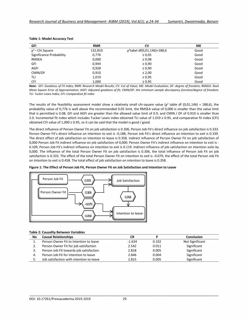
Research Journal of Business and Management -RJBM (2019), Vol.6(1). p.24-34 Sumantri, Dwiatmadja, Banani
_____________________________________________________________________________________ DOI: 10.17261/Pressacademia.2019.1019 29
Table 1: Model Accuracy Test
GFI RMR CV ME
χ2 – Chi Square Significance Probability RMSEA GFI AGFI CMIN/DF TLI CFI
132,810 0,776 0,000 0,944 0,928 0,910 1,019 1,000
χ2tabel df(0,01,146)=188,6 ≥ 0,05 ≤ 0,08 ≥ 0,90 ≥ 0,90 ≤ 2,00 ≥ 0,95 ≥ 0,95
Good Good Good Good Good Good Good Good
Note: GFI: Goodness of Fit Index; RMR: Research Model Results; CV: Cut of Value; ME: Model Evaluation; DF: degree of freedom; RMSEA: Root Mean Square Error of Approximation; AGFI: Adjusted goodness of fit; CMIN/DF: the minimum sample discrepancy function/degree of freedom; TLI: Tucker Lewis Index; CFI: Comparative fit index
The results of the feasibility assessment model show a relatively small chi-square value (χ2 table df (0,01,146) = 188,6), the probability value of 0,776 is well above the recommended 0.05 limit, the RMSEA value of 0,000 is smaller than the value limit that is permitted is 0.08, GFI and AGFI are greater than the allowed value limit of 0.9, and CMIN / DF of 0.910 is smaller than 2.0. Incremental fit index which includes Tucker Lewis index obtained TLI value of 1.019 ≥ 0.95, and comparative fit index (CFI) obtained CFI value of 1,000 ≥ 0.95, so it can be said that the model is good / good.
The direct influence of Person Owner Fit on job satisfaction is 0.306, Person Job Fit's direct influence on job satisfaction is 0.333. Person Owner Fit's direct influence on intention to exit is -0,188, Person Job Fit's direct influence on intention to exit is 0.339. The direct effect of job satisfaction on intention to leave is 0.358. Indirect influence of Person Owner Fit on job satisfaction of 0,000 Person Job Fit indirect influence on job satisfaction of 0,000. Person Owner Fit's indirect influence on intention to exit is -0.109, Person Job Fit's indirect influence on intention to exit is 0.119. Indirect influence of job satisfaction on intention exits by 0,000. The influence of the total Person Owner Fit on job satisfaction is 0.306, the total influence of Person Job Fit on job satisfaction is 0.333. The effect of the total Person Owner Fit on Intention to exit is -0.079, the effect of the total Person Job Fit on Intention to exit is 0.458. The total effect of job satisfaction on intention to leave is 0.358.
Figure 1: The Effect of Person Job Fit, Person Owner Fit on Job Satisfaction and Intention to Leave
Table 2: Causality Between Variables
No Causal Relationships CR P Conclusion
1. 2. 3. 4. 5.
Person Owner Fit to Intention to leave Person Owner Fit for job satisfaction Person Job Fit towards job satisfaction Person Job Fit for Intention to leave Job satisfaction with intention to leave
-1.634 2.542 2.818 2.846 2.815
0.102 0.011 0.005 0.004 0.005
Not Significant Significant Significant Significant Significant
Job Satisfaction
0,358
Intention to leave
0,333
0.306
0,458
-0.079

Research Journal of Business and Management -RJBM (2019), Vol.6(1). p.24-34 Sumantri, Dwiatmadja, Banani
_____________________________________________________________________________________ DOI: 10.17261/Pressacademia.2019.1019 30
From the results of calculations using AMOS 18 it can be concluded that hypothesis 1 is partially accepted, meaning that the dimensions of the Person Owner Fit has a negative influence on the intention to leave the company, but it is not significant because the value of p> 0.05. Hypotheses 2 and 3 are accepted. Hypothesis 4 is partly accepted because Person Job Fit has a significant influence on intention to leave but has a positive effect. Hypothesis 5 is partly accepted, this is because job satisfaction has a significant influence on intention to leave but has a positive effect.
4.2. Discussion
As mention at the objective of the research, this study examines two dimensions of conformity to see its effect on job satisfaction and intention to leave at the individual level. Testing is carried out on employees who work in micro and small businesses to see the perceptions of employee suitability with business owners. Both dimensions are assessed separately not to assess multidimensional constructs of conformity as proposed by Jansen and Kristof-Brown (2006), but as other alternative forms of assessing conformity.
The results show that Person Owner Fit has a negative effect on Intention to come out but is not significant. So the suitability of the individual with the owner can reduce the employee's intention to come out even though it is not significant. In relation to employee job satisfaction the results show that the Person Owner Fit has a positive and significant influence, this condition is reflected in the length of time the employee works in the place where they currently work. The Person Job Fit dimension shows a positive and significant influence on employee job satisfaction and intention to leave, meaning that conformity with work leads to perceived job satisfaction by employees. The desire to be able to work in a larger company is also another factor that is considered by employees and triggers the desire to leave their place of work at this time.
By looking at these results, the aspect of conformity with the owner is an important factor in supporting multidimensional conformity. In the first year new employees seek information about new organizations to assess their suitability (Chatman, 1991), but then they will shift their focus to more dynamic aspects such as compatibility with work and the people around them. The ASA framework model suggests that someone can be attracted to a place, maybe they made a mistake so they found a discrepancy that caused them to leave" (Schneider, 1987), thus producing more homogeneity in those who remain (Schneider et al., 1995).
One interesting finding is that the suitability of individuals and owners has a significant effect on job satisfaction, in contrast to the results stated (J. A. Edwards & Billsberry, 2010) in assessing conformity between individuals shows a standard regression weight that is very low and almost negligible in the equation, especially with the intention to leave and satisfaction. Other important factors can also determine perceptions of conformity, for example, people working alongside them, customers, staff, and other individuals they meet regularly (Kristof‐Brown, Zimmerman, et al., 2005), so that the dimensions of employee suitability with owners need to be included in multidimensional fit.
4.3. Implications
Person Owner Fit and Person Job Fit can be recommended in supporting employee job satisfaction and reducing the intention or desire of employees to leave the company. The focus of suitability in the Person Owner Fit dimension places more emphasis on employee personality aspects with the owner's personality and the suitability of the employee's lifestyle with the owner's lifestyle, while conformity in the Person Job Fit dimension emphasizes the appropriateness of the employee's ability to the demands of the work and existing work.
4.4. Research Limitations
The main limitations of this study only use a cross-sectional design, so that further testing is needed in replicating the findings with longitudinal data. In assessing conformity, it is done by using self-reported steps or subjective judgments. This action is said to have more economic benefits than other types of data collection (Cable & Judge, 1996, 1997; Kristof-Brown, 1996) but it is necessary to consider a more objective assessment. The sample used is only limited to MSMEs in Banyumas Indonesia with the business sector in the food processing and trading industry, so it needs to be developed in a wider scope so that more varied results can be obtained in assessing the suitability of individuals with their owners.
5. CONCLUSION
The Person Owner Fit dimension is a new dimension that adds multidimensional conformity in the Person Environment Fit theory, so the theory can be applied to organizations with various business scales. The development of the Person Owner Fit dimension is an important aspect because it can be used to assess the suitability that can affect employees in their intention to leave the workplace and influence their job satisfaction.

Research Journal of Business and Management -RJBM (2019), Vol.6(1). p.24-34 Sumantri, Dwiatmadja, Banani
_____________________________________________________________________________________ DOI: 10.17261/Pressacademia.2019.1019 31
REFERENCES
Adkins, C. L., Russell, C. J., Werbel, J. D. (1994). Judgments of fit in the selection process: The role of work value congruence. Personnel Psychology, 47(3), 605-623.
Aggarwal, U., Bhargava, S. (2010). Predictors and Outcomes of Relational and Transactional Psychological Contract. Psychological Studies, 55(3), 195-207. doi:10.1007/s12646-010-0033-2
Antonioni, D., Park, H. (2001). The effects of personality similarity on peer ratings of contextual work behaviors. Personnel Psychology, 54(2), 331-360.
Ashkanasy, N. M., O'connor, C. (1997). Value congruence in leader-member exchange. The Journal of Social Psychology, 137(5), 647-662.
Badan Pusat Statistik, Kabupaten Banyumas. (2017). In.
Bauer, T. N., Green, S. G. (1996). Development of leader-member exchange: A longitudinal test. Academy of management Journal, 39(6), 1538-1567.
Belk, R. W. (1988). Possessions and the extended self. Journal of consumer research, 15(2), 139-168.
BI, U. (2011). Kelayakan Pendirian Lembaga Pemeringkat Kredit Bagi Usaha Mikro, Kecil, Dan Menengah Di Indonesia: Bank Indonesia.
Blau, P. M. (1964). Exchange and power in social life: Transaction Publishers.
Brayfield, A. H., Rothe, H. F. (1951). An index of job satisfaction. Journal of applied psychology, 35(5), 307.
Brief, A. P., Weiss, H. M. (2002). Organizational behavior: Affect in the workplace. Annual review of psychology, 53(1), 279-307.
Cable, D. M., DeRue, D. S. (2002). The convergent and discriminant validity of subjective fit perceptions. Journal of applied psychology, 87(5), 875.
Cable, D. M., Judge, T. A. (1996). Person–organization fit, job choice decisions, and organizational entry. Organizational behavior and human decision processes, 67(3), 294-311.
Cable, D. M., Judge, T. A. (1997). Interviewers' perceptions of person–organization fit and organizational selection decisions. Journal of applied psychology, 82(4), 546.
Cammann, C., Fichman, M., Jenkins, D., Klesh, J. (1979). The Michigan organizational assessment questionnaire. Unpublished manuscript, University of Michigan, Ann Arbor.
Caplan, R. D. (1983). Person-environment fit: Past, present, and future. Stress research, 35(78), 173-187.
Cardon, M. S., Stevens, C. E. (2004). Managing human resources in small organizations: What do we know? Human resource management review, 14(3), 295-323.
Chatman, J. A. (1989). Improving interactional organizational research: A model of person-organization fit. Academy of management Review, 14(3), 333-349.
Chatman, J. A. (1991). Matching people and organizations: Selection and socialization in public accounting firms. Paper presented at the Academy of Management proceedings.
Chen, X.-P., Hui, C., Sego, D. J. (1998). The role of organizational citizenship behavior in turnover: Conceptualization and preliminary tests of key hypotheses. Journal of applied psychology, 83(6), 922.
Chuang, A., Judge, T. A., Liaw, Y. J. (2012). Transformational leadership and customer service: A moderated mediation model of negative affectivity and emotion regulation. European Journal of Work and Organizational Psychology, 21(1), 28-56.
Chuang, A., Shen, C. T., Judge, T. A. (2016). Development of a multidimensional instrument of person – environment fit: The Perceived Person – Environment Fit Scale (PPEFS). Applied Psychology, 65(1), 66-98.
Colbert, A. E. (2004). Understanding the effects of transformational leadership: The mediating role of leader-follower value congruence.
Dabos, G. E., Rousseau, D. M. (2004). Mutuality and reciprocity in the psychological contracts of employees and employers. Journal of Applied Psychology, 89(1), 52.
Dimarco, N. (1975). Life style, work group structure, compatibility, and job satisfaction. Academy of Management journal, 18(2), 313-322.
Dittmar, H. (1992). The social psychology of material possessions: To have is to be: Harvester Wheatsheaf and St. Martin's Press.
Donaldson, L., Davis, J. H. (1991). Stewardship theory or agency theory: CEO governance and shareholder returns. Australian Journal of management, 16(1), 49-64.
Edwards, J. A., Billsberry, J. (2010). Testing a multidimensional theory of person-environment fit. Journal of Managerial Issues, 476-493.

Research Journal of Business and Management -RJBM (2019), Vol.6(1). p.24-34 Sumantri, Dwiatmadja, Banani
_____________________________________________________________________________________ DOI: 10.17261/Pressacademia.2019.1019 32
Edwards, J. R. (1991). Person-job fit: A conceptual integration, literature review, and methodological critique: John Wiley & Sons.
Edwards, J. R. (1996). An examination of competing versions of the person-environment fit approach to stress. Academy of management Journal, 39(2), 292-339.
Edwards, J. R. (2008). 4 person–environment fit in organizations: an assessment of theoretical progress. Academy of Management Annals, 2(1), 167-230.
Engle, E. M., Lord, R. G. (1997). Implicit theories, self-schemas, and leader-member exchange. Academy of management Journal, 40(4), 988-1010.
Ferdinand, T. A. (2006). Metode Penelitian Manajemen: Pedoman Penulisan Skripsi. Tesis,dan Disertasi Ilmu Manajemen, (Vol. ed.1.). Semarang: BP-UNDIP.
Filotheos Ntalianis, L. D., Christian Vandenberghe. (2015). Owner-employee relations in small firms. Journal of Managerial Psychology, Vol. 30 Iss 7, 832 - 846. doi:10.1108/JMP-01-2013-0028
10.1108/JMP-03-2013-0088
French, J. R. (1974). Adjustment as person-environment fit. Coping and adaptation.
French, J. R., Kahn, R. L. (1962). A programmatic approach to studying the industrial environment and mental health. Journal of social issues, 18(3), 1-47.
Gatewood, R. D., Feild, H. S. (1987). A personnel selection program for small business. journal of small business management, 25(4), 16.
George;, J. M., Jones, G. R. (2012). Understanding and managing organizational behavior (6 ed.). New Jersey: Prentice Hall.
Graen, G., Cashman, J. F. (1975). A role-making model of leadership in formal organizations: A developmental approach. Leadership frontiers, 143, 165.
Graves, L. M., Powell, G. N. (1995). The Effect of sex similarity on recruiters'evaluations of actual applicants: a test of the similarity‐attraction paradigm. Personnel Psychology, 48(1), 85-98.
Harrison, D. A. (2007). Pitching fits in applied psychological research: making fit methods I-‘it theory. Perspectives on organizational fit, 389.
Hoffman, B. J., Bynum, B. H., Piccolo, R. F., Sutton, A. W. (2011). Person-organization value congruence: How transformational leaders influence work group effectiveness. Academy of Management Journal, 54(4), 779-796.
Holland, J. L. (1997). Making vocational choices: A theory of vocational personalities and work environments: Psychological Assessment Resources.
Hom, P. W., Griffeth, R. W. (1995). Employee Turnover (South-Western, Cincinnati, OH).
Homans, G. C. (1958). Social behavior as exchange. American journal of sociology, 63(6), 597-606.
House, R. J., Shane, S. A., Herold, D. M. (1996). Rumors of the death of dispositional research are vastly exaggerated. Academy of management review, 21(1), 203-224.
Ilies, R., Judge, T. A. (2002). Understanding the dynamic relationships among personality, mood, and job satisfaction: A field experience sampling study. Organizational Behavior and Human Decision Processes, 89(2), 1119-1139.
Jack, S., Hyman, J., Osborne, F. (2006). Small entrepreneurial ventures culture, change and the impact on HRM: A critical review. Human resource management review, 16(4), 456-466.
James, W. (1890). The Principles of Psychology (Vol. 2). New York, NY: Holt.
Jaramillo, F., J. P. Mulki., Solomon, P. (2006). The role of ethical climate on salesperson’s role stress, job attitudes, turnover intention, and job performance. Journal of Personal Selling and Sales Management, 26(3), 271-282.
Judge, T. A., Larsen, R. J. (2001). Dispositional affect and job satisfaction: A review and theoretical extension. Organizational Behavior and Human Decision Processes, 86(1), 67-98.
Krishnan, V. R. (2002). Transformational leadership and value system congruence. International Journal of Value-Based Management, 15(1), 19-33.
Kristof-Brown, A. L. (1996). Person‐organization fit: An integrative review of its conceptualizations, measurement, and implications. Personnel Psychology, 49(1), 1-49.
Kristof-Brown, A. L., Guay, R. P. (2011). Person–Environment Fit.

Research Journal of Business and Management -RJBM (2019), Vol.6(1). p.24-34 Sumantri, Dwiatmadja, Banani
_____________________________________________________________________________________ DOI: 10.17261/Pressacademia.2019.1019 33
Kristof-Brown, A. L., Stevens, C. K. (2001). Goal congruence in project teams: Does the fit between members' personal mastery and performance goals matter? Journal of applied psychology, 86(6), 1083-1095.
Kristof‐Brown, A. L. (2000). Perceived Applicant Fit: Distinguishing Between Recruiters' perceptions Of Person‐Job And Person‐Organization Fit. Personnel Psychology, 53(3), 643-671.
Kristof‐Brown, A. L., Barrick, M. R., Kay Stevens, C. (2005). When opposites attract: a multi‐sample demonstration of complementary person‐team fit on extraversion. Journal of Personality, 73(4), 935-958.
Kristof‐Brown, A. L., Zimmerman, R. D., Johnson, E. C. (2005). Consequences of individuals'fit at work: a meta analysis of person job, person organization, person group, and person supervisor fit. Personnel Psychology, 58(2), 281-342.
Kroeger, N. W. (1995). Person-Environment Fit in the Final Jobs of Retirees. The Journal of Social Psychology, 135(5), 545-551. doi:10.1080/00224545.1995.9712227
Lauver, K. J., Kristof-Brown, A. (2001). Distinguishing between employees' perceptions of person–job and person–organization fit. Journal of Vocational Behavior, 59(3), 454-470.
Li, C.-K., Hung, C.-H. (2010). An examination of the mediating role of person-job fit in relations between information literacy and work outcomes. Journal of Workplace Learning, 22(5), 306-318.
Liden, R. C., Wayne, S. J., Stilwell, D. (1993). A longitudinal study on the early development of leader-member exchanges. Journal of applied psychology, 78(4), 662.
Lincoln, J. R., Miller, J. (1979). Work and friendship ties in organizations: A comparative analysis of relation networks. Administrative Science Quarterly, 181-199.
Locke, E. A. (1976). The nature and causes of job satisfaction. Handbook of industrial and organizational psychology.
Matlay, H. (1999). Employee relations in small firms: A micro-business perspective. Employee relations, 21(3), 285-295.
Meglino, B. M., Ravlin, E. C., Adkins, C. L. (1991). Value congruence and satisfaction with a leader: An examination of the role of interaction. Human Relations, 44(5), 481-495.
Miles, R. E. (1964). Attitudes toward management theory as a factor in managers’ relationships with their superiors. Academy of management Journal, 7(4), 308-314.
Millward, L. J., Brewerton, P. M. (1999). Contractors and their psychological contracts. British Journal of management, 10(3), 253-274.
Montes, S. D., Irving, P. G. (2008). Disentangling the effects of promised and delivered inducements: relational and transactional contract elements and the mediating role of trust. Journal of Applied Psychology, 93(6), 1367.
Moos, R. H. (1987). Person-environment congruence in work, school, and health care settings. Journal of Vocational Behavior, 31(3), 231-247.
Muchinsky, P. M., Monahan, C. J. (1987). What is person-environment congruence? Supplementary versus complementary models of fit. Journal of Vocational Behavior, 31(3), 268-277.
O'Reilly, C. A., Caldwell, D. F., Barnett, W. P. (1989). Work group demography, social integration, and turnover. Administrative Science Quarterly, 21-37.
Parsons, F. (1909). Choosing a vocation: Houghton Mifflin.
Phillips, A. S., Bedeian, A. G. (1994). Leader-follower exchange quality: The role of personal and interpersonal attributes. Academy of management Journal, 37(4), 990-1001.
Piasentin, K. A., Chapman, D. S. (2007). Perceived similarity and complementarity as predictors of subjective person‐organization fit. Journal of Occupational and Organizational Psychology, 80(2), 341-354.
Randolph, D. S., Johnson, S. P. (2005). Predicting the effect of extrinsic and intrinsic job satisfaction factors on recruitment and retention of rehabilitation professionals. Journal of Healthcare management, 50(1), 49.
Rynes, S. L., Gerhart, B. (1993). Recruiter perceptions of applicant fit: Implications for individual career preparation and job search behavior. Journal of Vocational Behavior, 43(3), 310-327.
Saari, L. M., Judge, T. A. (2004). Employee attitudes and job satisfaction. Human Resource Management: Published in Cooperation with the School of Business Administration, The University of Michigan and in alliance with the Society of Human Resources Management, 43(4), 395-407.
Sabanciogullari, S., Dogan, S. (2015). Relationship between job satisfaction, professional identity and intention to leave the profession among nurses in Turkey. J Journal of nursing management, 23(8), 1076-1085.
Sartika, T., Soedjoedono, A. R. (2002). Ekonomi Skala Kecil/Menengah dan Koperasi. Ghalia Indonesia. Jakarta.

Research Journal of Business and Management -RJBM (2019), Vol.6(1). p.24-34 Sumantri, Dwiatmadja, Banani
_____________________________________________________________________________________ DOI: 10.17261/Pressacademia.2019.1019 34
Schaubroeck, J., Lam, S. S. (2002). How similarity to peers and supervisor influences organizational advancement in different cultures. Academy of management Journal, 45(6), 1120-1136.
Schneider, B. (1987). The people make the place. Personnel Psychology, 40(3), 437-453.
Schneider, B., Goldstiein, H. W., & Smith, D. B. (1995). The ASA framework: An update. Personnel Psychology, 48(4), 747-773.
Spanjol, J., Tam, L., Tam, V. (2015). Employer–employee congruence in environmental values: An exploration of effects on job satisfaction and creativity. J Journal of Business Ethics, 130(1), 117-130.
Steiner, D. D., Dobbins, G. (1989). The role of work values in leaders' attributions and the development of leader-member exchanges. International Journal of Management, 6(1), 81-90.
Super, D. E. (1953). A theory of vocational development. American psychologist, 8(5), 185.
Tsui, A. S., O'reilly, C. A. (1989). Beyond simple demographic effects: The importance of relational demography in superior-subordinate dyads. Academy of management Journal, 32(2), 402-423.
Turban, D. B., Dougherty, T. W. (1994). Role of protégé personality in receipt of mentoring and career success. Academy of management Journal, 37(3), 688-702.
Turban, D. B., Jones, A. P. (1988). Supervisor-subordinate similarity: types, effects, and mechanisms. Journal of applied psychology, 73(2), 228.
Valentine, S., Godkin, L., Fleischman, G. M., Kidwell, R. (2011). Corporate ethical values, group creativity, job satisfaction and turnover intention: The impact of work context on work response. Journal of business ethics, 98(3), 353-372.
Vianen, A. E. (2000). Person‐organization fit: The match between newcomers'and recruiters'preferences for organizational cultures. Personnel Psychology, 53(1), 113-149.
Walker, E., Brown, A. (2004). What success factors are important to small business owners? International small business journal, 22(6), 577-594.
Wang, M., Zhan, Y., McCune, E., Truxillo, D. (2011). Understanding newcomers’adaptability and work‐related outcomes: Testing the mediating roles of perceived P–E fit variables. Personnel psychology, 64(1), 163-189.
Werbel, J. D., Gilliland, S. W. (1999). Person–environment fit in the selection process.
Williamson, O. E. (1981). The economics of organization: The transaction cost approach. American journal of sociology, 87(3), 548-577.
Witt, L. (1998). Enhancing organizational goal congruence: A solution to organizational politics. Journal of applied psychology, 83(4), 666.
Yu, K. Y. T. (2016). Inter‐Relationships among different types of Person–Environment fit and job satisfaction. J Applied Psychology, 65(1), 38-65.

Research Journal of Business and Management- RJBM (2019), Vol6(1). p.35-45 Chen, Fang
________________________________________________________________________________________________________ DOI: 10.17261/Pressacademia.2019.1020 35
JOB STRESSORS AND JOB PERFORMANCE: MODELING OF MODERATING MEDIATION EFFECTS OF STRESS MINDSET DOI: 10.17261/Pressacademia.2019.1020 RJBM- V.6-ISS.1-2019(4)-p.35-45
Hsiao-Ling Chen1, Shih-Chieh Fang2 1 National Cheng Kung University, Department of Business Administration, No.1, University Road, Tainan City 701, Taiwan (R.O.C). [email protected], ORCID: 0000-0002-2459-127 2 National Cheng Kung University, Department of Business Administration, No.1, University Road, Tainan City 701, Taiwan (R.O.C). [email protected], ORCID: 0000-0001-5006-8677
Date Received: December 8, 2018 Date Accepted: March 6, 2019
To cite this document Chen, H.-L., Fang, S.-C. (2019). Job stressors and job performance: Modeling of moderating mediation effects of stress mindset. Research Journal of Business and Management (RJBM), V.6(1), p.35-45. Permemant link to this document: http://doi.org/10.17261/Pressacademia.2019.1020 Copyright: Published by PressAcademia and limited licenced re-use rights only.
ABSTRACT Purpose - Job stress is widely concern to academic researcher and practitioner, work stress may affect employee attitudes and physical and mental health. We proposed that person’s appraisal plays a critical role in the stress process, although the nature of job stress is sometimes to make people grow, sometimes make people shrink, but we believe that individual perception of stressors is the key factor affecting the follow-up behaviors. This study examines the moderated effect of stress mindset on the indirect relationship between job stressors and job performance mediated by job satisfaction. We integrated the transactional theory of stress and the concept of stress mindset, try to provide another explanation of boundary condition for the ambiguous results in the relation between stressors and job satisfaction. Methodology - Research participants were general employees and their supervisors, data were collected from 487 employees from the different occupation in Taiwan, including trading company, restaurants, travel agency, bank, salesperson and staff of gas station and train station. Statistical analyses using SPSS and Mplus for model testing, the results show that there exists a moderated mediation effect. For measurement model of stress mindset, we conducted two-factor CFA to examine whether the eight items were loaded onto two factor. The result indicated that the data fit the two-factor model better than one-factor model. For structure model of research framework, the results supporting the independence of the six focal constructs, results indicated that the six-factor model fit the data better than the other models. Findings - First, our results suggested that job sastisfaction mediated the positive relationship between challenge stressors and job performance, also mediated the negative relationship between hindrance stressors and job performance. Second, the positive relationship between challenge stressors and outcomes stronger when negative stress mindset is low, and negative relationship between hindrance stressors and outcomes weaker when positive stress mindset is high. Conclusion - This study integrates the transactional theory of stress and the concept of stress mindset to investigate the moderating mediation model. Our findings reveal that individual’s different stress mindset of stressors plays a critical moderating role during the process of pursuit working goal. Once individual hold a negative stress mindset, the positive mediation will become weaker; reversely, holding a positive stress mindset can help the negative mediation become weaker. Based on the research findings, implications and suggestions for theoretical and practical implication are discussed.
Keywords: Challenge stressors, hindrance stressors, negative stress mindset, positive stress mindset, job satisfaction. JEL Codes: D23, J28, M12

Research Journal of Business and Management- RJBM (2019), Vol6(1). p.35-45 Chen, Fang
________________________________________________________________________________________________________ DOI: 10.17261/Pressacademia.2019.1020 36
1. INTRODUCTION
The issue of job stress is widely concern to academic researcher and practitioner. Kahn, Wolfe, Quinn, Snoek, and Rosenthal (1964) introduced the concept of stressors into organization and management research areas, organizational scholars have increasingly discussed stressors at workplace and developed stress management techniques. Mostly early studies stated that stress is harmful, and has a negative impact on organization and individuals, people must adopt effective strategies to prevent or reduce the incidence of stress (Atkinson, 2004; Bodenmann, Meuwly, Bradbury, Gmelch, & Ledermann, 2010; McEwen & Seeman, 1999; Schwabe & Wolf, 2010). Cooper, Dewe, and O’Driscoll (2001) argued that work stress may affect employee attitudes and physical and mental health. However, prior studies mostly focused on the negative impact of stress but ignored the positive effect of stress may exist.
Some stressors in the workplace contain the elements of growth, can be opportunities for individuals to enhance performance, but some stressors erode employee’s passion of the work, may hinder the effectiveness of work. Cavanaugh, Boswell, Roehling, and Boudreau (2000) followed inverted U-shape model (Selye, 1982) and transactional theory of stress (Lazarus & Folkman, 1984), classified job stressors as challenge stressors and hindrance stressors. Challenge stressors have potential growth opportunities for individuals, can guide individual to invest effort into solving problems, result in positive consequences, such as higher job satisfaction (Cavanaugh et al., 2000; Podsakoff, LePine, & LePine, 2007; Webster, Beehr, & Christiansen, 2010); engagement (Crawford, LePine, & Rich, 2010) and performance (LePine, Podsakoff, & LePine, 2005); but lower turnover (Cavanaugh et al., 2000; Podsakoff et al., 2007). Conversely, hindrance stressors will make people stuck with job demand, reduce their work motivation and bring negative results (Podsakoff et al., 2007), such as higher turnover intention, withdraw behaviors (Cavanaugh et al., 2000; Podsakoff et al., 2007), and physical symptoms (Webster et al., 2010); but lower job satisfaction (Cavanaugh et al., 2000; Podsakoff et al., 2007; Webster et al., 2010), engagement (Crawford et al., 2010); motivation (LePine et al., 2005) and job performance (LePine et al., 2005; Pearsall, Ellis, & Stein, 2009; Wallace, Edwards, Arnold, Frazier, & Finch, 2009).
However, according to transactional theory of stress (Lazarus & Folkman, 1984), person’s appraisal plays a critical role in the stress process. Although the nature of job stress is sometimes to make people grow, sometimes make people shrink, but we believe that individual perception of stressors is the key factor affecting the follow-up behaviors. Existing research focused less on the moderating effect of individual mindset that affects individual behaviors. Therefore, we considered the boundary conditions in the relationship between stressors and outcomes by introduced the concept of stress mindset, refers as the extent to which one holds the belief that stress has enhancing or debilitating results (Crum, Salovey, & Achor, 2013).
This study contributes to stress research in some ways. First, we integrate the transactional theory of stress and the concept of stress mindset, provide another viewpoint in stress issues. Second, we extend the concept of stress mindset proposed by Crum et al. (2013), which further divided into positive and negative stress mindset. Finally, we give another explanation of boundary condition for the ambiguous results in the relation between stressors and job satisfaction.
2. LITERATURE REVIEW
2.1. Transactional Theory of Stress
Lazarus and Folkman (1984) proposed transactional theory of stress, defined as an individual’s psychological response to a critical situation and where the situation taxes or exceeds the individual’s capacity or resources can offer, it is considered a product of the transaction between the individual and the environment. Central to the transactional theory of stress is the idea of cognitive appraisal, namely primary appraisal and secondary appraisal. Lazarus and Folkman (1984, 1986) using concepts from expectancy theory (Vroom, 1964), suggested that the initial appraisal process of stressors triggers specific emotional reactions and coping styles that in turn influence behaviors. Primary appraisal is to recognize that situation stressors are potential harm or benefit to the self. Secondary appraisal is then concerned with identifying the appropriate response or coping ways to the specific stressors.
2.2. Challenge and Hindrance Stressors
Cavanaugh et al. (2000) followed Selye (1982) and Lazarus and Folkman’s (1984, 1986) work, suggested that job stressors have negative and positive effects on work outcomes. They classified work stressors into “challenge” and “hindrance” stressors. Challenge stressors were defined as “work-related demands or circumstances that, although potentially stressful, have associated potential gains for individuals”, such as workload, time pressure, job responsibility, and job complexity. Hindrance stressors were defined as “work-related demands or circumstances that tend to constrain or interfere with an individual's work

Research Journal of Business and Management- RJBM (2019), Vol6(1). p.35-45 Chen, Fang
________________________________________________________________________________________________________ DOI: 10.17261/Pressacademia.2019.1020 37
achievement and that do not tend to be associated with potential gains for the individual”, for instances, role ambiguity, role conflict, hassles, red tape, organizational politics, and job insecurity (Cavanaugh et al., 2000, p. 68).
Existing studies shown that challenge stressors are positively related to job attitude, such as job satisfaction (Cavanaugh et al., 2000; Podsakoff et al., 2007; Webster et al., 2010), loyalty (Boswell, Olson-Buchanan, & LePine, 2004), organizational commitment (Podsakoff et al., 2007), engagement (Crawford et al., 2010); cognition, such as motivation (LePine et al., 2005), self-efficacy (Webster et al., 2010), organizational justice (Zhang, LePine, Buckman, & Wei, 2014); and behaviors, such as performance (LePine et al., 2005), role-based performance (task performance, citizenship performance, and customer service performance; Wallace et al., 2009). But, negative effects on job attitude, such as intention to quit (Boswell et al., 2004), turnover intention (Podsakoff et al., 2007); and behaviors, such as job search (Boswell et al., 2004; Cavanaugh et al., 2000), turnover (Cavanaugh et al., 2000; Podsakoff et al., 2007), and work withdrawal behavior (Boswell et al., 2004).
On the other hand, hindrance stressors are positively related to job attitude, such as intention to quit (Boswell et al., 2004), turnover intention (Podsakoff et al., 2007), psychological withdrawal (Pearsall et al., 2009); and behaviors, such as job search (Boswell et al., 2004; Cavanaugh et al., 2000), turnover (Cavanaugh et al., 2000; Podsakoff et al., 2007), withdraw behaviors (Podsakoff et al., 2007), physical symptoms (Webster et al., 2010). Hindrance stressors also have negative effects on job attitude, such as job satisfaction (Cavanaugh et al., 2000; Podsakoff et al., 2007; Webster et al., 2010), loyalty (Boswell et al., 2004), organizational commitment (Podsakoff et al., 2007), engagement (Crawford et al., 2010); cognition, such as motivation (LePine et al., 2005), self-efficacy (Webster et al., 2010), organizational justice (Zhang et al., 2014); and behaviors, such as performance (LePine et al., 2005), role-based performance (task performance, citizenship performance, and customer service performance; Wallace et al., 2009), and team performance (Pearsall et al., 2009).
Job satisfaction refers to a psychological state resulting from the evaluation of one’s job experiences (Locke, 1976). Based on transactional theory of stress and challenge-hindrance framework, challenge stressors have potential gains for individuals, it should be positively associated with attitudinal and behavioral outcomes. Conversely, hindrance stressors have potential for harm or failure, it is likely to be negatively associated with attitudinal and behavioral outcomes (LePine et al., 2005; Webster et al., 2010; Webster, Beehr, & Love, 2011). According to Lazarus and Folkman (1984), individual will activate initial appraisal process when they face stressors and trigger positive or negative emotional reactions in turn influence behaviors. Challenge stressors provide potential growth opportunities for employees, active employee’s enthusiasm for work and positively affect job satisfaction. Conversely, hindrance stressors tend to interfere with employee’s work achievement and negatively affect job satisfaction. Prior studies supported that challenge stressors will positively but hindrance stressors will negatively affect job satisfaction (Podsakoff et al., 2007; Webster et al., 2010) and both challenge stressors and hindrance stressors were positively effect on job performance (LePine et al., 2005). We argued that job satisfaction will mediate the effects of stressors on job performance (Fried, Shirom, Gilboa, & Cooper, 2008), and employees who are satisfied with their jobs will enhance their performance in jobs, the recent study also found the similar evidence (Nasir, Khan, & Nasir, 2017). Thus, we proposed hypothesis 1 and 2 as follow.
Hypothesis 1: Job satisfaction mediates the positive relationship between challenge stressors and job performance.
Hypothesis 2: Job satisfaction mediates the negative relationship between hindrance stressors and job performance.
2.3. Stress Mindset
“Mindset” defines as a mental frame or lens of what we selectively organize and encode information, and guide individual’s corresponding actions and responses by a unique way of understanding (Dweck, 2008). Crum et al. (2013) bring the concept of mindset into the field of stress, stress mindset is the extent to which an individual holds the conviction that stress has enhancing or debilitating. They suggested that change one’s stress mindset can improve people's response to stress. Specifically, if individual holds a stress-is-enhancing mindset, the primary motivation is to accept and utilize stress toward achieving their goals, brings positive consequence. On the other hand, if individual holds a stress-is-debilitating mindset, the primary motivation is to avoid or manage the stress to prevent negative or debilitating outcomes.
Although two types of stressors affect opposite consequences, existing research found that both challenge and hindrance stressors are positively related to psychological strain (anxiety and emotional exhaustion; Boswell et al., 2004), exhaustion (LePine, LePine, & Jackson, 2004), strain (LePine et al., 2005; Podsakoff et al., 2007), anxiety (Rodell & Judge, 2009), frustration (Webster et al., 2010), burnout (Crawford et al., 2010). According to review paper of Podsakoff et al. (2007), we agree that both challenge stressors and hindrance stressors will increase psychological strain and strain will negatively lead to job satisfaction. However, the mediator variable for strain does not explain that how challenge stressors positively affects job satisfaction and

Research Journal of Business and Management- RJBM (2019), Vol6(1). p.35-45 Chen, Fang
________________________________________________________________________________________________________ DOI: 10.17261/Pressacademia.2019.1020 38
hindrance stressors is negative effect on job satisfaction. We believe that individual’s perception of stressors may play an important moderating variable.
The stress mindset measure is developed by Crum et al. (2013), they treated stress-is-enhancing and stress-is-debilitating mindset as the continuum, thus higher score of scale means one’s holds stress-is-enhancing, and lower score means mindset of stress-is-debilitating. However, we think that stress mindset should be two independent factors, hence we separated their measure into positive and negative stress mindset. The individual holds positive stress mindset can bring benefit results, but negative stress mindset will bring damage results. We argue that even though challenge stressors can bring positive outcomes, but if individual hold negative stress mindset, the positive relationship will be debilitating. Even stressors were recognized as promoting growth, negative perception of stressors will damage employee’s job satisfaction and the potential successful performance. Reversely, even hindrance stressors will constrain individuals’ development and performance, once individual can hold positive stress mindset, at least employee will try to solve the problem. If they think there still have chance to invest effort, depends on our appraisal of how we perceived stressors is helpful or harmful. This can reduce the negative relationship between hindrance stressors and job satisfaction and performance. Thus, we proposed hypothesis 3 and 4 as follow.
Hypothesis 3: Negative stress mindset (NSM) will moderate the positive indirect effect of challenge stressors and job performance mediated by job satisfaction. When NSM is high, the positive indirect effect weakens; when NSM is low, the positive indirect effect is stronger.
Hypothesis 4: Positive stress mindset (PSM) will moderate the negative indirect effect of hindrance stressors and job performance mediated by job satisfaction. When PSM is high, the negative indirect effect weakens; when PSM is low, the negative indirect effect is stronger.
Figure 1: Research Model
3. DATA AND METHODOLOGY
3.1. Sample and Procedure
The research participants were general employees and their supervisors. Randomized sampling was used to 530 employees from different occupation, including trading company, restaurants, travel agency, bank, salesperson and staff of gas station and train station in Taiwan. After uncompleted questionnaires were excluded, a final sample was 487 questionnaires was used for data analyses. The employees’ demographics showed that 57.6% were females, with an average age of 26.10 years and average work tenure of 4.94 years. Most were single (85.2%) with college education level (76.3%).
3.2. Measure
Challenge and hindrance stressors. Cavanaugh et al. (2000) challenge-hindrance stressors scale was used in our study. There are 6 items measured challenge stressors, a sample item was “The amount of time I spend at work.” The Cronbach’s alpha coefficient was 0.81. On the other hand, 5 items measured hindrance stressors, a sample item was “The lack of job security I have.” The Cronbach’s alpha coefficient was 0.73.
Positive and negative stress mindset. We measured stress mindset using the stress mindset measure–general (SMM-G) 8-item scale of Crum et al. (2013), but we treated original four of eight positive items as positive stress mindset and the other four inverted items as negative stress mindset. A sample item of positive stress mindset was “Experiencing stress facilitates my
Challenge Stressors
Job Satisfaction Job Performance
Negative Stress Mindset
Hindrance Stressors
Positive Stress Mindset
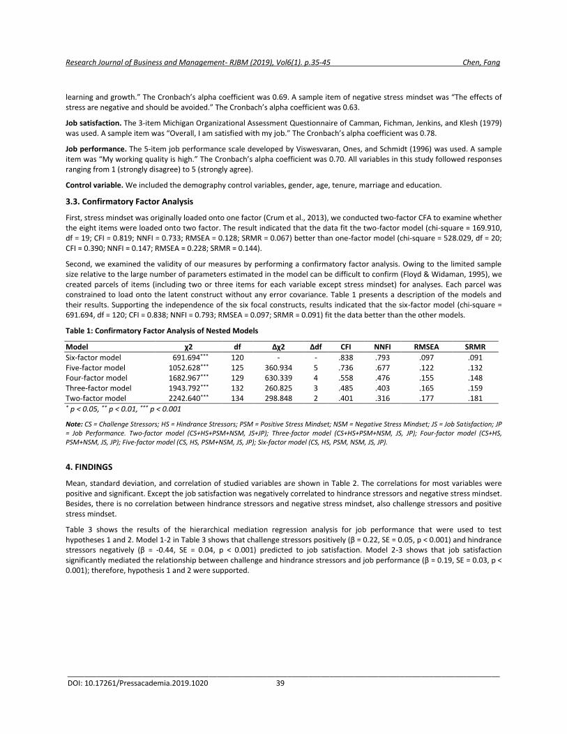
Research Journal of Business and Management- RJBM (2019), Vol6(1). p.35-45 Chen, Fang
________________________________________________________________________________________________________ DOI: 10.17261/Pressacademia.2019.1020 39
learning and growth.” The Cronbach’s alpha coefficient was 0.69. A sample item of negative stress mindset was “The effects of stress are negative and should be avoided.” The Cronbach’s alpha coefficient was 0.63.
Job satisfaction. The 3-item Michigan Organizational Assessment Questionnaire of Camman, Fichman, Jenkins, and Klesh (1979) was used. A sample item was “Overall, I am satisfied with my job.” The Cronbach’s alpha coefficient was 0.78.
Job performance. The 5-item job performance scale developed by Viswesvaran, Ones, and Schmidt (1996) was used. A sample item was “My working quality is high.” The Cronbach’s alpha coefficient was 0.70. All variables in this study followed responses ranging from 1 (strongly disagree) to 5 (strongly agree).
Control variable. We included the demography control variables, gender, age, tenure, marriage and education.
3.3. Confirmatory Factor Analysis
First, stress mindset was originally loaded onto one factor (Crum et al., 2013), we conducted two-factor CFA to examine whether the eight items were loaded onto two factor. The result indicated that the data fit the two-factor model (chi-square = 169.910, df = 19; CFI = 0.819; NNFI = 0.733; RMSEA = 0.128; SRMR = 0.067) better than one-factor model (chi-square = 528.029, df = 20; CFI = 0.390; NNFI = 0.147; RMSEA = 0.228; SRMR = 0.144).
Second, we examined the validity of our measures by performing a confirmatory factor analysis. Owing to the limited sample size relative to the large number of parameters estimated in the model can be difficult to confirm (Floyd & Widaman, 1995), we created parcels of items (including two or three items for each variable except stress mindset) for analyses. Each parcel was constrained to load onto the latent construct without any error covariance. Table 1 presents a description of the models and their results. Supporting the independence of the six focal constructs, results indicated that the six-factor model (chi-square = 691.694, df = 120; CFI = 0.838; NNFI = 0.793; RMSEA = 0.097; SRMR = 0.091) fit the data better than the other models.
Table 1: Confirmatory Factor Analysis of Nested Models
Model χ2 df ∆χ2 ∆df CFI NNFI RMSEA SRMR
Six-factor model 691.694*** 120 - - .838 .793 .097 .091 Five-factor model 1052.628*** 125 360.934 5 .736 .677 .122 .132 Four-factor model 1682.967*** 129 630.339 4 .558 .476 .155 .148 Three-factor model 1943.792*** 132 260.825 3 .485 .403 .165 .159 Two-factor model 2242.640*** 134 298.848 2 .401 .316 .177 .181 * p < 0.05, ** p < 0.01, *** p < 0.001
Note: CS = Challenge Stressors; HS = Hindrance Stressors; PSM = Positive Stress Mindset; NSM = Negative Stress Mindset; JS = Job Satisfaction; JP = Job Performance. Two-factor model (CS+HS+PSM+NSM, JS+JP); Three-factor model (CS+HS+PSM+NSM, JS, JP); Four-factor model (CS+HS, PSM+NSM, JS, JP); Five-factor model (CS, HS, PSM+NSM, JS, JP); Six-factor model (CS, HS, PSM, NSM, JS, JP).
4. FINDINGS
Mean, standard deviation, and correlation of studied variables are shown in Table 2. The correlations for most variables were positive and significant. Except the job satisfaction was negatively correlated to hindrance stressors and negative stress mindset. Besides, there is no correlation between hindrance stressors and negative stress mindset, also challenge stressors and positive stress mindset.
Table 3 shows the results of the hierarchical mediation regression analysis for job performance that were used to test hypotheses 1 and 2. Model 1-2 in Table 3 shows that challenge stressors positively (β = 0.22, SE = 0.05, p < 0.001) and hindrance stressors negatively (β = -0.44, SE = 0.04, p < 0.001) predicted to job satisfaction. Model 2-3 shows that job satisfaction significantly mediated the relationship between challenge and hindrance stressors and job performance (β = 0.19, SE = 0.03, p < 0.001); therefore, hypothesis 1 and 2 were supported.

Research Journal of Business and Management- RJBM (2019), Vol6(1). p.35-45 Chen, Fang
________________________________________________________________________________________________________ DOI: 10.17261/Pressacademia.2019.1020 40
Table 2: Means, Standard Deviations, and Correlations among All Variables Studied
Variables Means SD 1 2 3 4 5 6 7 8 9 10 11
1.Gender 1.58 .50 -
2.Age 26.03 10.71 .03 -
3.Tenure 4.94 7.87 .05 .88*** -
4.Marriage 1.15 .36 .06 .81*** .74*** -
5.Education 2.84 .53 .09 .02 -.09 -.08 -
6.CS 3.60 .62 .02 .21*** .16*** .16*** .14** (.81) 7.HS 2.72 .68 .00 .04 .03 .05 .02 .22*** (.73) 8.PSM 3.62 .56 -.05 -.08 -.09* -.11* .05 .25*** .01 (.69) 9.NSM 3.06 .68 -.04 .03 .02 .03 -.08 .06 .32*** .13** (.63) 10.JS 3.64 .70 -.01 .07 .06 .08 .10* .11* -.38*** .37*** -.19*** (.78) 11.JP 3.57 .54 -.01 .15** .13** .08 .12** .56*** .12** .38*** .18*** .27*** (.70) * p < 0.05, ** p < 0.01, *** p < 0.001
Note: N=487. Reliabilities are reported in parentheses. CS = Challenge Stressors; HS = Hindrance Stressors; PSM = Positive Stress Mindset; NSM = Negative Stress Mindset; JS = Job Satisfaction; JP = Job Performance.
Table 3: Results of Mediation Regression Analysis
Job Satisfaction Job Performance
Model 1-1 Model 1-2 Model 2-1 Model 2-2 Model 2-3
Control Variable
Gender -.05 (.06) -.05 (.06) -.03 (.05) -.03 (.04) -.02 (.04)
Age -.00 (.01) -.00 (.01) .01 (.01) .00 (.01) .00 (.01)
Tenure .01 (.01) .00 (.01) .00 (.01) .01 (.01) .01 (.01)
Marriage .16 (.16) .21 (.14) -.10 (.12) -.10 (.10) -.14 (.10)
Education .16 (.06)** .14 (.06)* .11 (.05)* .04 (.04) .02 (.04)
Independent Variable
Challenge Stressors .22 (.05)*** .47 (.03)*** .43 (.03)***
Hindrance Stressors -.44 (.04)*** -.01 (.03) .07 (.03)*
Mediator
Job Satisfaction .19 (.03)***
R2 .02 .20 .04 .32 .37
F 1.98 17.40*** 3.80** 31.97*** 34.73***
ΔR2 .18 .28 .05
ΔF 54.84*** 98.54*** 37.18*** * p < 0.05, ** p < 0.01, *** p < 0.001 Note: The regression coefficient is unstandardized coefficient and stander error is reported in parentheses.
Regarding hypothesis 3 and 4, we expected NSM would have a moderating effect on the first stage of hypothesis 1 and PSM would have a moderating effect on the first stage of hypothesis 2. The results of hierarchical moderation regression analysis were shown in Table 4. Model 4 in Table 4 shows that the interaction term of challenge stressors and NSM has a significant negative effect on job satisfaction (β = -0.07, SE = 0.02, p < 0.01); and another interaction term of hindrance stressors and PSM has a significant positive effect on job satisfaction (β = 0.06, SE = 0.02, p < 0.01). We also conducted a hierarchical moderating mediation regression analysis by using Mplus 7.0, the result as shown in Table 5.
First, Table 5 shows the interaction term of challenge stressors and NSM has a significant negative moderated effect on job satisfaction (β = -0.18, SE = 0.06, p < 0.01). We have plotted this interaction at conditional values of NSM (1 SD above and below the mean) in Figure 2. This graph indicates that the positive indirect relationship between challenge stressors and job performance mediated by job satisfaction is stronger when NSM is low, therefore, hypothesis 3 was supported. On the other

Research Journal of Business and Management- RJBM (2019), Vol6(1). p.35-45 Chen, Fang
________________________________________________________________________________________________________ DOI: 10.17261/Pressacademia.2019.1020 41
hand, Table 5 also shows another interaction term of hindrance stressors and PSM has a significant positive moderated effect on job satisfaction (β = 0.16, SE = 0.07, p < 0.05). We also plotted this interaction at conditional values of PSM (1 SD above and below the mean) in Figure 3. This graph indicates that the negative indirect relationship between hindrance stressors and job performance mediated by job satisfaction is stronger when PSM is low, therefore, hypothesis 4 was supported.
Second, to further determine whether NSM and PSM weakened the indirect relationship as predicted by Hypothesis 1 and 2, we considered an alternative moderated mediation model, including the first stage, second stage, direct, indirect, and total effects of the moderator (NSM and PSM). The NSM results shown in Table 6 indicate a pattern consistent with our prediction, with significant effects in the first stage effect (diffidence β = 0.240, SE = 0.078, p < 0.01); therefore, hypothesis 3 was supported. The PSM results shown in Table 7, also consistent with our prediction, with significant effects in the first stage effect (diffidence β = -0.174, SE = 0.073, p < 0.05); therefore, hypothesis 4 was supported.
5. CONCLUSION AND DISCUSSIONS
This study integrates the transactional theory of stress and the concept of stress mindset to investigate the moderating mediation model. First, our results suggested that job satisfaction mediated the positive relationship between challenge stressors and job performance, also mediated the negative relationship between hindrance stressors and job performance. Second, we introduce concept of stress mindset proposed by Crum et al. (2013), and further divided into positive and negative stress mindset. Our findings reveal that individual’s different stress mindset of stressors plays a critical moderating role during the process of pursuit working goal. Once individual hold a negative stress mindset, the positive mediation will become weaker; reversely, holding a positive stress mindset can help the negative mediation become weaker.
Table 4: Results of Moderation Regression Analysis
Job Satisfaction
Control Variable Model 1 Model 2 Model 3 Model 4
Gender -.05 (.06) -.05 (.06) -.04 (.05) -.04 (.05)
Age -.00 (.01) -.00 (.01) -.00 (.01) -.00 (.01)
Tenure .01 (.01) .00 (.01) .00 (.01) .00 (.01)
Marriage .16 (.16) .21 (.14) .30 (.13)* .32 (.13)*
Education .16 (.06)** .14 (.06)* .12 (.05)* .14 (.05)**
Independent Variable
CS .13 (.03)*** .05 (.03)† .05 (.03)†
HS -.30 (.03)*** -.26 (.03)*** -.25 (.03)***
Moderator
PSM .28 (.03)*** .28 (.03)***
NSM -.09 (.03)** -.08 (.03)**
Interaction
CS*PSM .12 (.02)
CS*NSM -.07 (.02)**
HS*PSM .06 (.02)**
HS*NSM -.02 (.02)
R2 .02 .20 .34 .36
F 1.98 17.40*** 27.53*** 20.81***
ΔR2 .18 .14 .02
ΔF 54.84*** 50.43*** 4.09** † p < 0.1, * p < 0.05, ** p < 0.01, *** p < 0.001
Note: CS = Challenge Stressors; HS = Hindrance Stressors; PSM = Positive Stress Mindset; NSM = Negative Stress Mindset. The regression coefficient is unstandardized coefficient and stander error is reported in parentheses.
5.1. Theoretical Implication
First, existing studies lack empirical evidence to link the relationship between challenge-hindrance framework, job satisfaction and job performance, and our study fills this research gap. According to the transactional theory of stress Lazarus and Folkman

Research Journal of Business and Management- RJBM (2019), Vol6(1). p.35-45 Chen, Fang
________________________________________________________________________________________________________ DOI: 10.17261/Pressacademia.2019.1020 42
(1984, 1986), individual will appraise the stressors they encounter, challenge stressors can trigger positive emotion and lead to positive outcomes; hindrance stressors will trigger negative emotion and result in bad outcomes. Our findings suggested that challenge stressors can positive affect job satisfaction and enhance job performance, but hindrance stressors will damage employee’s job satisfaction and reduce job performance, which extends the existing studies (Fried et al., 2008; LePine et al., 2005; Podsakoff et al., 2007; Webster et al., 2010).
Second, Crum et al. (2013) bring concept of mindset into stress issue, they suggested that one’s mindset tend to stress-is-enhancing will lead to positive consequence; conversely, one’s mindset tend to stress-is-debilitating will lead to negative outcomes. We agree with Crum et al. (2013), and argue that different stress mindset can result in different behaviors. However, we don’t agree with Crum et al. (2013) the methodological way they employed which treated stress mindset as a spectrum, the degree of stress-is-enhancing or stress-is-debilitating. We divided stress mindset scale into positive and negative two factors, and the result of the confirmatory factor analysis also supports our idea. Therefore, we refined Crum et al. (2013) stress mindset measures, provide future researchers with another option.
Furthermore, we give an explanation for the ambiguous results in the relation between two types of stressors and job satisfaction (Podsakoff et al., 2007). Result shows that stress mindset is a boundary condition that moderates the relationship between stressors and job satisfaction. Even challenge stressors were recognized as “good” stress and can lead to beneficial consequence, but if one’s hold negative stress mindset, this positive relationship will be impaired. Conversely, hindrance stressors was treated as “bad” stress and brings damage outcomes, but if employee can hold positive stress mindset, this negative relationship will be repaired.
Table 5: Moderated Mediation Model Results
Job Satisfaction Job Performance
Intercepts -.62 (.23)** 3.56 (.14)***
Control variables Gender -.04 (.05) -.01 (.04) Age -.00 (.01) .00 (.01) Tenure .00 (.01) .01 (.01) Marriage .32 (.16)* -.09 (.09) Education .14 (.06)* .03 (.04)
Independent variables
CS .08 (.05) .38 (.04)***
HS -.37 (.05)*** .01 (.04)
Mediator JS .15 (.05)**
Moderator PSM .50 (.06)** .15 (.05)** NSM -.12 (.05)* .14 (.04)***
Interaction
CS*PSM .03 (.07) .01 (.08)
CS*NSM -.18 (.06)** -.02 (.05)
HS*PSM .16 (.07)* -.01 (.09)
HS*NSM -.04 (.05) .01 (.05)
JS*PSM -.02 (.08)
JS*NSM -.12 (.07)† † p < 0.1, * p < 0.05, ** p < 0.01, *** p < 0.001
Note: CS = Challenge Stressors; HS = Hindrance Stressors; JS = Job Satisfaction; PSM = Positive Stress Mindset; NSM = Negative Stress Mindset. The estimate is unstandardized coefficient and stander error is reported in parentheses.

Research Journal of Business and Management- RJBM (2019), Vol6(1). p.35-45 Chen, Fang
________________________________________________________________________________________________________ DOI: 10.17261/Pressacademia.2019.1020 43
Table 6: Overview of Significant Moderated Mediation Effects for Negative Stress Mindset
First Stage Effect Second Stage Effect Direct Effect Indirect Effect Total Effect
Low_ NSM (-1 SD) .197 (.053)*** .232 (.082)** .391 (.055)*** .046 (.021)* .437 (.052)***
High_ NSM (+1 SD) -.043 (.074) .073 (.049) .366 (.053)*** -.003 (.007) .363 (.054)***
Diffidence .240 (.078)** .159 (.093)† .025 (.072) .049 (.020)* .074 (.069) † p < 0.1, * p < 0.05, ** p < 0.01, *** p < 0.001 Note: NSM = Negative Stress Mindset (SD= .67780). Standard errors are reported in parentheses.
Table 7: Overview of Significant Moderated Mediation Effects for Positive Stress Mindset
First Stage Effect Second Stage Effect Direct Effect Indirect Effect Total Effect
Low_ PSM (-1 SD) -.456 (.070)*** .162 (.068)* .021 (.076) -.074 (.030)* -.053 (.065)
High_ PSM (+1 SD) -.282 (.055)*** .143 (.067)* .008 (.051) -.040 (.018)* -.032 (.047)
Diffidence -.174 (.073)* .019 (.093) .013 (.101) -.034 (.034) -.021 (.083) * p < 0.05, ** p < 0.01, *** p < 0.001 Note: PSM = Positive Stress Mindset (SD= .56233). Standard errors are reported in parentheses.
5.2. Empirical Implication
Our findings suggested that job satisfaction mediated the relationship between challenge/hindrance stressors and job performance. In practice, the organization should try to provide employee more growth and development opportunities for the job, such as setting timeliness of task completion, increase job responsibility or complexity of task, these challenge stressors can make working situation become more challenging. This paper also presents that stress mindset can affect individuals’ attitudes and consequent behaviors. Consequently, organization could assist employee to establish positive mindset or develop positive thinking by organize learning activity or set up psychological counseling units to help employees rethink the stressors they faced.
5.3. Limitations and Suggestion for Future Research
There are still some research limitations in this study. First, our research variables are derived from employee self-reporting, may lead to common methods variance concerns, especially job performance may have inflation effect. We suggest future study should use supervisor-employee dyad questionnaire to exclude common sources concerns. Second, we divided stress mindset scale into two factors without pilot study to ensure the reliability of the scale. Although the confirmatory factor analysis shows
Figure 1: Negative stress mindset (NSM) moderates the mediation effect of job satisfaction between challenge stressors (CS) and job performance.
Figure 2: Positive stress mindset (PSM) moderates the mediation effect of job satisfaction between hindrance stressors (HS) and job performance.

Research Journal of Business and Management- RJBM (2019), Vol6(1). p.35-45 Chen, Fang
________________________________________________________________________________________________________ DOI: 10.17261/Pressacademia.2019.1020 44
two-factor model is preferred, but we recommended the follow-up studies should be categorized in a more rigorous manner. Third, our sample only for Taiwanese employees, the results may not be enough to generalize to other countries, suggesting that future research should increase the research sample to increase the external validity.
REFERENCES
Atkinson, W. (2004). Stress: Risk management's most serious challenge? Risk Management, 51(6), 20-26.
Bodenmann, G., Meuwly, N., Bradbury, T. N., Gmelch, S., Ledermann, T. (2010). Stress, anger, and verbal aggression in intimate relationships: Moderating effects of individual and dyadic coping. Journal of Social and Personal Relationships, 27(3), 408-424.
Boswell, W. R., Olson-Buchanan, J. B., LePine, M. A. (2004). Relations between stress and work outcomes: The role of felt challenge, job control, and psychological strain. Journal of Vocational Behavior, 64(1), 165-181. doi:10.1016/S0001-8791(03)00049-6
Camman, C., Fichman, M., Jenkins, D., Klesh, J. (1979). The Michigan organizational assessment questionnaire. University of Michigan. Ann Arbor, MI.
Cavanaugh, M. A., Boswell, W. R., Roehling, M. V., Boudreau, J. W. (2000). An empirical examination of self-reported work stress among U.S. managers. Journal of Applied Psychology, 85(1), 65-74. doi:10.1037//0021-9010.85.1.65
Cooper, C. L., Dewe, P., O’Driscoll, M. P. (2001). Organizational stress: A review and critique of theory, research and applications: SAGE Publications, Inc.
Crawford, E. R., LePine, J. A., Rich, B. L. (2010). Linking job demands and resources to employee engagement and burnout: A theoretical extension and meta-analytic test. Journal of Applied Psychology, 95(5), 834-848.
Crum, A. J., Salovey, P., Achor, S. (2013). Rethinking stress: The role of mindsets in determining the stress response. Journal of Personality and Social Psychology, 104(4), 716-733. doi:10.1037/a0031201
Dweck, C. S. (2008). Can personality be changed? The role of beliefs in personality and change. Current Directions in Psychological Science, 17(6), 391-394. doi:10.1111/j.1467-8721.2008.00612.x
Floyd, F. J., Widaman, K. F. (1995). Factor analysis in the development and refinement of clinical assessment instruments. Psychological Assessment, 7(3), 286-299.
Fried, Y., Shirom, A., Gilboa, S., Cooper, C. L. (2008). The mediating effects of job satisfaction and propensity to leave on role stress-job performance relationships: Combining meta-analysis and structural equation modeling. International Journal of Stress Management, 15(4), 305-328.
Kahn, R. L., Wolfe, D. M., Quinn, R. P., Snoek, J. D., Rosenthal, R. A. (1964). Organizational stress: Studies in role conflict and ambiguity. Oxford, England: John Wiley.
Lazarus, R. S., Folkman, S. (1984). Stress, appraisal, and coping. New York: Springer Publishing Company.
Lazarus, R. S., Folkman, S. (1986). Cognitive theories of stress and the issue of circularity. In M. H. Appley & R. Trumbull (Eds.), Dynamics of Stress: Physiological, Psychological and Social Perspectives (pp. 63-80). Boston, MA: Springer US.
LePine, J. A., LePine, M. A., Jackson, C. L. (2004). Challenge and hindrance stress: Relationships with exhaustion, motivation to learn, and learning performance. Journal of Applied Psychology, 89(5), 883-891. doi:10.1037/0021-9010.89.5.883
LePine, J. A., Podsakoff, N. P., LePine, M. A. (2005). A meta-analytic test of the challenge stressor–hindrance stressor framework: An explanation for inconsistent relationships among stressors and performance. Academy of Management Journal, 48(5), 764-775. doi:10.5465/amj.2005.18803921
Locke, E. A. (1976). The nature and causes of job satisfaction. In M. D. Dunnette (Ed.), Handbook of industrial and organizational psychology (pp. 1297-1343). Chicago, IL: Rand McNally.
McEwen, B. S., Seeman, T. (1999). Protective and damaging effects of mediators of stress: Elaborating and testing the concepts of allostasis and allostatic load. Annals of the New York Academy of Sciences, 896(1), 30-47. doi:10.1111/j.1749-6632.1999.tb08103.x
Nasir, N., Khan, S., Nasir, S. (2017). Workplace stressors and job performance: The hypothesized mediating role of job satisfaction incase of higher educational sector of pakistan. International Journal of Engineering Sciences & Research Technology, 6(2), 609-623.
Pearsall, M. J., Ellis, A. P. J., Stein, J. H. (2009). Coping with challenge and hindrance stressors in teams: Behavioral, cognitive, and affective outcomes. Organizational Behavior and Human Decision Processes, 109(1), 18-28. doi:10.1016/j.obhdp.2009.02.002
Podsakoff, N. P., LePine, J. A., LePine, M. A. (2007). Differential challenge stressor-hindrance stressor relationships with job attitudes, turnover intentions, turnover, and withdrawal behavior: A meta-analysis. Journal of Applied Psychology, 92(2), 438-454. doi:10.1037/0021-9010.92.2.438

Research Journal of Business and Management- RJBM (2019), Vol6(1). p.35-45 Chen, Fang
________________________________________________________________________________________________________ DOI: 10.17261/Pressacademia.2019.1020 45
Rodell, J. B., Judge, T. A. (2009). Can “good” stressors spark “bad” behaviors? The mediating role of emotions in links of challenge and hindrance stressors with citizenship and counterproductive behaviors. Journal of Applied Psychology, 94(6), 1438-1451.
Schwabe, L., Wolf, O. T. (2010). Learning under stress impairs memory formation. Neurobiol Learn Mem, 93(2), 183-188. doi:10.1016/j.nlm.2009.09.009
Selye, H. (1982). History and present status of the stress concept. In L. Goldberger & S. Breznitz (Eds.), Handbook of stress: Theoretical and clinical aspects (pp. 7-17). New York: Free Press.
Viswesvaran, C., Ones, D. S., Schmidt, F. L. (1996). Comparative analysis of the reliability of job performance ratings. Journal of Applied Psychology, 81(5), 557-574.
Vroom, V. H. (1964). Work and motivation. New York: Wiley.
Wallace, J. C., Edwards, B. D., Arnold, T., Frazier, M. L., Finch, D. M. (2009). Work stressors, role-based performance, and the moderating influence of organizational support. Journal of Applied Psychology, 94(1), 254-262. doi:10.1037/a0013090
Webster, J. R., Beehr, T. A., Christiansen, N. D. (2010). Toward a better understanding of the effects of hindrance and challenge stressors on work behavior. Journal of Vocational Behavior, 76(1), 68-77. doi:10.1016/j.jvb.2009.06.012
Webster, J. R., Beehr, T. A., Love, K. (2011). Extending the challenge-hindrance model of occupational stress: The role of appraisal. Journal of Vocational Behavior, 79(2), 505-516. doi:10.1016/j.jvb.2011.02.001.
Zhang, Y., LePine, J. A., Buckman, B. R., Wei, F. (2014). It's not fair … or is it? The role of justice and leadership in explaining work stressor–job performance relationships. Academy of Management Journal, 57(3), 675-697. doi:10.5465/amj.2011.1110.

Research Journal of Business and Management -RJBM (2019), Vol.6(1). p.46-67 Chen, Wei, Che
__________________________________________________________________________________ DOI: 10.17261/Pressacademia.2019.1021 46
DOES PATENT CONTRIBUTE TO STOCK PRICE IN CHINA?
DOI: 10.17261/Pressacademia.2019.1021 RJBM- V.6-ISS.1-2019(5)-p.46-67
Tsui-Min Chen1, Chiu-Chi Wei2, Hui-Chung Che3 1 Chung Hua University, Ph.D. Program of Technology Management, 707, Sec.2, WuFu Rd., Hsinchu, Taiwan. [email protected], ORCID: 0000-0003-0617-8902 2 Chung Hua University, Industrial Management, 707, Sec.2, WuFu Rd., Hsinchu, Taiwan. [email protected], ORCID: 0000-0002-9433-9114 3 Shenzhen TekGlory IP Data Technologies, Room 201, Site A, Qianwan 1st Rd., Shenzhen, Quandong, China. [email protected] , ORCID: 0000-0003-2873-1510
Date Received: December 15, 2018 Date Accepted: March 8, 2018
To cite this document Chen, C. H., Wei, C. C., Che, H. C. (2019). Does patent contribute to stock price in China?. Research Journal of Business and Management (RJBM), V.6(1), p.46-67. Permemant link to this document: http://doi.org/10.17261/Pressacademia.2019.1021 Copyright: Published by PressAcademia and limited licenced re-use rights only.
ABSTRACT Purpone - Along with the in-depth implementation of national intellectual property strategies in China, China’s intellectual property law has been fully integrated with international norms. The number of patents in China is among the highest in the world and China has been the country with the largest number of patent applications in the world for five consecutive years. In addition, the incentive and protective role of the intellectual property system on economy, science, technology and culture has emerged. Methodology - There are more than 3,000 A-share listed companies in mainland China, as the second largest stock market among global transactions, with the daily trading volume exceeding one trillion RMB. Its ups and downs are catching the eyes of global investors. Patents are the concrete manifestations of scientific and technological innovations. It is questionable if this specific performance can contribute to financial performance and if investment potential stocks can be exploited through patent indicators. In view of this, in this study, an empirical research was conducted on the data of the technology-based enterprises listed on the Shanghai A-share market from 2011 to 2017. Findings - It is found in this study that, compared to stock prices, there is a significant leading period of specific patent indicators for more than one year. After the data back-testing of the stock exchange, the average performance of the investment potential stocks selected based on this research model is better than the market index performance. Conclusion - Though the statistical test and time series algorithm of patent indicators, the leading patent formulas are deduced in this study, which can validly predict the stock price of listed companies and the lead period is up to one year, at least a quarter with predictive accuracy.
Keywords: Patent, patent indicator, stock price, forecasts, panel data, Granger causality test. JEL Codes: O34, P14
1. INTRODUCTION
According to the "World Economic Situation and Prospects 2018" issued by the United Nations, one-third of global economic growth in 2017 was contributed from China. There are more than 3,000 A-share listed companies in mainland China, with the daily trading volume over 1 trillion RMB, so that the Chinese stock market is the second largest stock market among global transactions and its ups and downs are driving the eyes of global investors.
Since patents have the benefit of protecting research and development results, companies tend to disclose their research and development results in the form of patents. Therefore, compared with disclosed papers on journal articles and technology, patent literatures provide a wealth of research and development information. According to the statistics of the World Intellectual Property Organization (WIPO), 90-95% of innovations worldwide can be searched in patent literatures (WIPO).
There is no doubt that patents are the concrete manifestations of scientific and technological innovations. However, can innovation results contribute to the financial performance of patent owners? If yes, how can it be measured specifically? If it can be measured, compared to financial information, does patent information belong to a leading indicator or a backward indicator? Such questions have not yet been answered completely in both theory and practice fields.

Research Journal of Business and Management -RJBM (2019), Vol.6(1). p.46-67 Chen, Wei, Che
__________________________________________________________________________________ DOI: 10.17261/Pressacademia.2019.1021 47
In the 1970s, the U.S. CHI Research and the U.S. National Science Foundation (NSF) jointly developed patent-based scientific achievement indicators. CHI Research's patent indicator system was used in the "Science and Engineering Indicators" published by NSF. Many academic studies pointed out that quantity information of patents leads ahead of the sales information of the leading product and thus it has a leading effect in explaining market developments. Consequently, the methods of predicting market trends with patent information have gradually become an important research topic in investment and business evaluation (Narin, 1995; Suh, 2015; Shassan, 2016).
In another aspect, due to large amounts and full disclosure of information in US patents, most of the previous academic articles were based on US patents for research and empirical analysis and related research on patents in mainland China was relatively scarce. However, with the continuous implementation of China’s national intellectual property strategy, China’s intellectual property laws have been fully integrated with international regulations. The number of patents in mainland China has been among the highest in the world and China has been the country with the largest number of patent applications in the world five consecutive years. At present, the number of patents accumulated has reached 22 million. The role of the intellectual property system in inspiring and guaranteeing the country's economy, science and technology and culture has also begun to appear. Based on such a condition, the causality and transformation of A shares and patents in mainland China has become a topic of great concern in countries, markets, societies, and enterprises.
The official name of China A shares is RMB common stocks, which refer to ordinary stocks registered and listed in China. China's A shares are mainly divided into 1389 Shanghai main boards, 465 Shenzhen main boards, 903 SME boards, 710 GEM boards, etc. Among them, Shanghai main boards not only have the largest number of companies but also the most state-owned enterprises, with more indicative meanings than other boards. Therefore, this study is aimed at a total of 1389 listed companies in Shanghai Main Board to explore the relevance and leadership of patent and financial data by collecting financial and patent data of listed companies from 2011 to 2017. Then, it is attempted to predict the stock price with patent data as a reference for investment stock selection.
This paper is composed of the following sections, the introduction, literature review, method, analysis and results and conclusion.
2. LITERATURE
In a patent specification, the patentee must fully disclose the substance and novelty of the technology in order to make patents be granted and thus enjoy the exclusiveness of the patent granted by the law. Once the patent is obtained, the patentee will be given the exclusive advantage during a specific time in the application market of the technology.
Patent indicators based on patent information extraction are different from general technology indicators but has a more substantial ability to observe technology trends (Ernst, 1995; Grag & Padhi, 1998,). Yan and Liang (2009) have sorted out the development of relevant patent indicators. They organized the definition and usage of patent indicators proposed by CHI Research and tried to use the quantified patent indicators to explain the company's technology trends and strengths. The Organization for Economic Co-operation and Development (OECD) used patent information to quantify it into patent indicators and divided it into three levels-national analysis indicators, industrial level analysis indicators and enterprise level analysis indicators. Ernst et al. (1997, 2001) published research on patent indicators in 2001 and specifically pointed out three types of patent indicators, including relative patent positioning indicators, technical attractiveness indicators, and technical importance indicators, which can be used as a basis for business management, R&D resource allocation, and strategic R&D planning.
There are many studies that confirm the utility of patent indicators in corporate financial projections. For example, KaiP (2009) targeted the profitability of the top 50%, the top 25%, and the top 10% of Danish companies and the company’s patent application activities. They conducted correlation analysis by F-test, regression analysis, etc. It was found that the number of patent applications has a significant positive correlation with the company's profit margin. Gao et al. (2013) proposed the S-curves to observe changes in the number of patent applications over time and construct a model to calculate the change in the life cycle of the technology based on multiple patent indicators, of which the results can facilitate investors to assess whether the company is worth investing.
The stock market's stock price forecast attracts many scholars or investors to engage in related research. Lin et al. (2006) found that there is a clear positive correlation in a company using patent portfolios and diversity with the company's investment performance, shareholders' equity and profit margin. Mazzucato et al. (2012) and Hirshleifer et al. (2013) pointed out that the innovation efficiency quantified by the patent indicators is positively correlated with the performance of the stock price. Zhang & Chen (2013) suggested that when the short-term effects of irrational factors are excluded, the stock price of a company is determined by factors such as the overall performance of the company or the ability of the decision makers to manage in the long run. Consequently, a company's stock price or its technological trends of the industry can be predicted through the overall performance of the company. Vitt & Xiong (2015) tried to use mathematical models to analyze the relationship between the stock price information of high-tech listed companies of NASDAQ in the

Research Journal of Business and Management -RJBM (2019), Vol.6(1). p.46-67 Chen, Wei, Che
__________________________________________________________________________________ DOI: 10.17261/Pressacademia.2019.1021 48
U.S. and the status of the company's patent activities. The research results proved that there was a positive correlation with two years of deferral between the company's stock price fluctuation and its patent activities.
In addition, patents are linked to long-term and sustainable profits since they represent innovation and realistic outcomes from research across different fields, countries, and periods of time (Trajtenberg 1990; Hullmann & Meyer, 2003). Jincheol et al. (2017) proposed patent-cited data to provide financial analysts with an assessment of the company's ability to innovate, which has a certain degree of accuracy and can further reduce the uncertainty of the inherent investment technology. Chen & Chang (2015) pointed out that the enterprises can make a good use of the continuation patent system on patent layouts to protect design patents while suppressing copying or imitating works of continuation patents
3. METHODOLOGY
First, in this paper, appropriate target company stock prices and patent data were collected. Then, the patent data were converted into patent indicators. Through Granger causality test, the sample data with a causal relationship with the stock prices were screened. Finally, by using multivariate regression of time sequence, a patent-leading equation that predicts stock prices was established. The details are as follows.
3.1 Research Steps
This research is aimed at technology-based enterprises with a sufficient number of patents in Shanghai main boards in mainland China. The research steps are shown in Figure 1. The steps are explained as follows:
(1) Collecting patent and share price information of listed companies: Shanghai Main Board's stock price data and corresponding mainland China’s patent data from 2011 to 2017 were collected.
(2) Defining patent indicators: mainland China’s patent indicators were defined and patent data of Shanghai Main Board companies are processed to generate patent indicators.
(3) Screening valid samples: the minimum patent number of Shanghai Main Board was set as a valid sample screening threshold and valid samples were screened out.
(4) Six panel data based on modeling period: a set of panel data in a modeling period of two years was formed respectively in the patent index and stock price of the valid sample of Shanghai Main Board and six groups of panel data were divided.
(5) Forming leading indicators of patents through Granger Causality Test: by using patent indicators as independent variables and stock market closing prices as the dependent variable, through the Granger causality test, the leading properties and leading periods of the patent indicators c relative to the stock market closing price in each group's panel data were explored; patent indicators with predictive significance was excavated and defined as leading patent indicators.
(6) Generating significant patent leading formulas: the significant patented leading equations were established in the leading patent indicators of each group through time series.
(7) Forecasting stock prices of each company: the predicted stock prices were calculated based on the patent leading equations in each modeling period.
(8) Calculating the expected rate of return.
(9) Verifying the performance of stock selection: annual and quarterly simulation investments were conducted based on the forecasted rate of return and the simulated investment performance was verified separately with the market average and the SSE Composite Index.
3.2 Limitation & Delimitation
1. The stock exchanges in mainland China include the Shanghai Stock Exchange and the Shenzhen Stock Exchange. In this study, the Shanghai main board was selected as the research object since it has more listed companies, a considerable number of state-owned enterprises, and a particularly strong amount of capital.
2. There are a total of 1389 companies in the Shanghai main boards used in this study. The closing prices of the stock market released on the last trading day of each quarter from 2011 to 2017 were collected as the stock price data for the season.

Research Journal of Business and Management -RJBM (2019), Vol.6(1). p.46-67 Chen, Wei, Che
__________________________________________________________________________________ DOI: 10.17261/Pressacademia.2019.1021 49
Figure 1: Research Flow Chart
3. If the financial statements of subsidiaries and sub-subsidiaries are also merged with the parent company in the listed company’s financial report, it is suggested in this study that the patents of subsidiaries and sub-subsidiaries should also be merged into the parent company. Therefore, this study is based on the list of subsidiaries and sub-subsidiaries disclosed in the semi-annual and annual reports of listed companies to conduct calculation by data processing merger to the parent company.
4. In this study, only the impact of mainland China’s patents on stock prices was considered. The patents outside mainland China were excluded, such as PCT patents, US patents, European patents, etc.
5. The original data of mainland China’s patents used in this study are the patent data published in the patent database of State Intellectual Property Office of the People's Republic of China (SIPO).
3.3. Instrumentation
3.3.1. Granger Causality Test
Granger Causality Test was developed by Granger, Clive W. J., the 2003 Nobel Prize in Economics (Granger, 1969; Granger, 1980), which is used to analyze Granger causality between economic variables. This is an econometric definition that defines the causal relationship in the sense of time series. To judge whether the independent variable X asscoiated with the dependent variable Y, it is needed to examine that the current value of the variable Y can be explained by the past value of the variable X and then to examine whether the adding of the hysteresis value of independent variable X can explain the degree of improvement. If the hysteresis value of the independent variable X helps to improve the degree of interpretation of the dependent variable Y, the independent variable X is considered to be the Granger cause of the dependent variable Y (Granger, 1969). That is, the dependent variable can be predicted by observing the independent variable X.
In specific operations, the hysteresis values of the independent variable X and the dependent variable Y are frequently used to formulate the regression equation. This is also checked by F Test and observing p values.
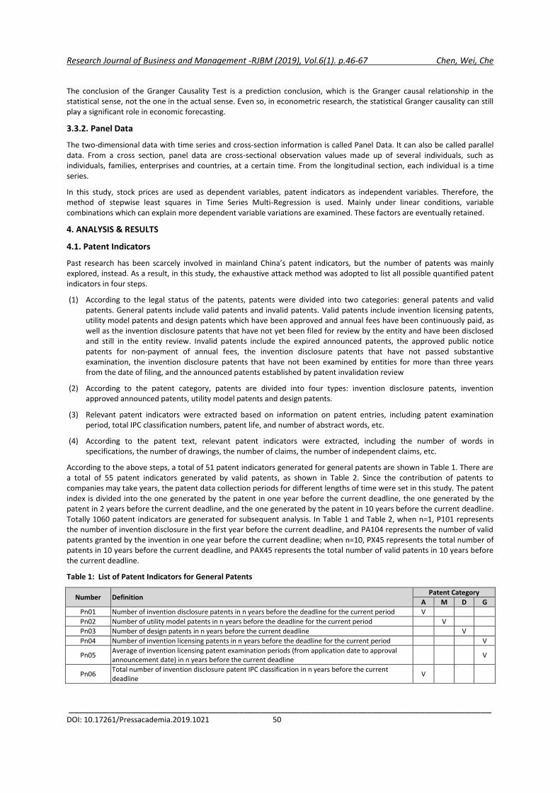
Research Journal of Business and Management -RJBM (2019), Vol.6(1). p.46-67 Chen, Wei, Che
__________________________________________________________________________________ DOI: 10.17261/Pressacademia.2019.1021 50
The conclusion of the Granger Causality Test is a prediction conclusion, which is the Granger causal relationship in the statistical sense, not the one in the actual sense. Even so, in econometric research, the statistical Granger causality can still play a significant role in economic forecasting.
3.3.2. Panel Data
The two-dimensional data with time series and cross-section information is called Panel Data. It can also be called parallel data. From a cross section, panel data are cross-sectional observation values made up of several individuals, such as individuals, families, enterprises and countries, at a certain time. From the longitudinal section, each individual is a time series.
In this study, stock prices are used as dependent variables, patent indicators as independent variables. Therefore, the method of stepwise least squares in Time Series Multi-Regression is used. Mainly under linear conditions, variable combinations which can explain more dependent variable variations are examined. These factors are eventually retained.
4. ANALYSIS & RESULTS
4.1. Patent Indicators
Past research has been scarcely involved in mainland China’s patent indicators, but the number of patents was mainly explored, instead. As a result, in this study, the exhaustive attack method was adopted to list all possible quantified patent indicators in four steps.
(1) According to the legal status of the patents, patents were divided into two categories: general patents and valid patents. General patents include valid patents and invalid patents. Valid patents include invention licensing patents, utility model patents and design patents which have been approved and annual fees have been continuously paid, as well as the invention disclosure patents that have not yet been filed for review by the entity and have been disclosed and still in the entity review. Invalid patents include the expired announced patents, the approved public notice patents for non-payment of annual fees, the invention disclosure patents that have not passed substantive examination, the invention disclosure patents that have not been examined by entities for more than three years from the date of filing, and the announced patents established by patent invalidation review
(2) According to the patent category, patents are divided into four types: invention disclosure patents, invention approved announced patents, utility model patents and design patents.
(3) Relevant patent indicators were extracted based on information on patent entries, including patent examination period, total IPC classification numbers, patent life, and number of abstract words, etc.
(4) According to the patent text, relevant patent indicators were extracted, including the number of words in specifications, the number of drawings, the number of claims, the number of independent claims, etc.
According to the above steps, a total of 51 patent indicators generated for general patents are shown in Table 1. There are a total of 55 patent indicators generated by valid patents, as shown in Table 2. Since the contribution of patents to companies may take years, the patent data collection periods for different lengths of time were set in this study. The patent index is divided into the one generated by the patent in one year before the current deadline, the one generated by the patent in 2 years before the current deadline, and the one generated by the patent in 10 years before the current deadline. Totally 1060 patent indicators are generated for subsequent analysis. In Table 1 and Table 2, when n=1, P101 represents the number of invention disclosure in the first year before the current deadline, and PA104 represents the number of valid patents granted by the invention in one year before the current deadline; when n=10, PX45 represents the total number of patents in 10 years before the current deadline, and PAX45 represents the total number of valid patents in 10 years before the current deadline.
Table 1: List of Patent Indicators for General Patents
Number Definition Patent Category
A M D G
Pn01 Number of invention disclosure patents in n years before the deadline for the current period V
Pn02 Number of utility model patents in n years before the deadline for the current period V
Pn03 Number of design patents in n years before the current deadline V
Pn04 Number of invention licensing patents in n years before the deadline for the current period V
Pn05 Average of invention licensing patent examination periods (from application date to approval announcement date) in n years before the current deadline
V
Pn06 Total number of invention disclosure patent IPC classification in n years before the current deadline
V

Research Journal of Business and Management -RJBM (2019), Vol.6(1). p.46-67 Chen, Wei, Che
__________________________________________________________________________________ DOI: 10.17261/Pressacademia.2019.1021 51
Pn07 Total number of utility model patent IPC classification in n years before the current deadline V
Pn08 Total number of invention licensing patent IPC classification in n years before the current deadline
V
Pn09 Average of invention disclosure patent IPC classification in n years before the current deadline V
Pn10 Average of utility model patent IPC classification in n years before the current deadline V
Pn11 Average of IPC classification numbers of invention licensing patents in n years before the deadline for the current period
V
Pn12 Total number of words in invention disclosure patent specifications in n years before the deadline for the current period
V
Pn13 Total number of words in utility model patent specifications in n years before the deadline for the current period
V
Pn14 Total number of words in the invention licensing patents in n years before the deadline for the current period
V
Pn15 Average of words in invention disclosure patents specifications in n years before the deadline for the current period
V
Pn16 Average of words in utility model patent specifications in n years before the deadline for the current period
V
Pn17 Average of words in invention licensing patent specifications in n years before the deadline for the current period
V
Pn18 Total number of claims of invention disclosure patents in n years before the deadline for the current period
V
Pn19 Total number of claims of utility model patents in n years before the deadline for the current period
V
Pn20 Total number of claims of invention licensing patents in n years before the deadline for the current period
V
Pn21 Average of claims of invention disclosure patents in n years before the deadline for the current period
V
Pn22 Average of claims of utility model patents in n years before the deadline for the current period V
Pn23 Average of claims of invention licensing patents in n years before the deadline for the current period
V
Pn24 Total number of exclusive claims of invention disclosure patents in n years before the deadline for the current period
V
Pn25 Total number of exclusive claims of utility model patents in n years before the deadline for the current period
V
Pn26 Total number of exclusive claims of invention licensing patents in n years before the deadline for the current period
V
Pn27 Average of exclusive claims of invention disclosure patents in n years before the deadline for the current period
V
Pn28 Average of exclusive claims of utility model patents in n years before the deadline for the current period
V
Pn29 Average of exclusive claims of invention licensing patents in n years before the deadline for the current period
V
Pn30 Total number of drawings in invention disclosure patent specifications in n years before the deadline for the current period
V
Pn31 Total number of drawings of utility model patents in n years before the deadline for the current period
V
Pn32 Total number of drawings in invention licensing patent specifications in n years before the deadline for the current period
V
Pn33 Average of drawings of invention disclosure patents in n years before the deadline for the current period
V
Pn34 Average of drawings in utility model patent specifications in n years before the deadline for the current period
V
Pn35 Average of drawings for invention licensing patents in n years before the deadline for the current period
V
Pn36 Total number of invention disclosure patent abstracts in n years before the deadline for the current period
V
Pn37 Total number of words in utility model abstracts in n years before the deadline for the current period
V
Pn38 Total number of invention licensing patent abstracts in n years before the deadline for the current period
V
Pn39 Average of disclosure patent abstracts in n years before the deadline for the current period V
Pn40 Average of utility model abstracts in n years before the deadline for the current period V
Pn41 Average of invention licensing patent abstracts in n years before the deadline for the current period
V

Research Journal of Business and Management -RJBM (2019), Vol.6(1). p.46-67 Chen, Wei, Che
__________________________________________________________________________________ DOI: 10.17261/Pressacademia.2019.1021 52
Pn45 Total number of patents in n years before the current deadline V V V V
Pn46 Proportion of invention disclosure patents in n years before the deadline for the current period V
Pn47 Proportion of utility model patents in n years before the deadline for the current period V
Pn48 Proportion of design patents in n years before the deadline for the current period V
Pn49 Proportion of invention licensing patents in n years before the deadline for the current period V
Pn50 Average life expectancy of invention disclosure patents in n years before the deadline for the current period
V
Pn51 Average life expectancy of utility model patents in n years before the deadline for the current period
V
Pn52 Average life expectancy of design patents in n years before the deadline for the current period V
Pn53 Average life expectancy of invention licensing patents in n years before the deadline for the current period
V
Pn54 Total number of invention pre-patent citations in n years before the deadline for the current period
V
Note: A: invention disclosure patents; M: utility model patents; D: design patents; G: invention licensing patents
Table 2: List of Patent Indicators for Valid Patents
Number Definition Patent Category
A M D G
PAn01 Number of valid invention disclosure patents in n years before the deadline for the current period V
PAn02 Number of valid utility model patents in n years before the deadline for the current period V
PAn03 Number of patents valid for design in n years before the deadline for the current period V
PAn04 Number of valid invention licensing patents in n years before the deadline for the current period V
PAn05 Average of the patent examination period for invention licensing patents in n years before the current deadline (from the date of application to the date of approval)
V
PAn06 Total number of valid invention disclosure patent IPC classification numbers in n years before the deadline for the current period
V
PAn07 Total number of valid utility model patent IPC classification numbers in n years before the deadline for the current period
V
PAn08 Total number of invention licensing patent IPC classification numbers in n years before the current deadline
V
PAn09 Average of valid invention disclosure patent IPC classification numbers in n years before the deadline for the current period
V
PAn10 Average of valid utility model patent IPC classification numbers in n years before the deadline for the current period
V
PAn11 Average of valid invention licensing patent IPC classification numbers in n years before the current deadline
V
PAn12 Total number of words of valid invention disclosure patents in n years before the deadline for the current period
V
PAn13 Total number of valid utility model patent specifications in n years before the deadline for the current period
V
PAn14 Total number of words in valid invention licensing patent specifications in n years before the current deadline
V
PAn15 Average of words of valid invention disclosure patents in n years before the deadline for the current period
V
PAn16 Average of valid utility model patent specifications in n years before the deadline for the current period
V
PAn17 Average of words in valid invention licensing patent specifications in n years before the deadline for the current period
V
PAn18 Total number of claims of valid invention disclosure patents in n years before the deadline for the current period
V
PAn19 Total number of claims of valid utility model patents in n years before the deadline for the current period
V
PAn20 Total number of claims of invention of valid invention licensing patents in n years before the deadline for the current period
V
PAn21 Average of claims of valid invention disclosure patents in n years before the deadline for the current period
V
PAn22 Average of claims of valid utility model patents in n years before the deadline for the current period
V
PAn23 Average of claims of valid invention licensing patent in n years before the deadline for the current period
V
PAn24 Total number of exclusive claims of valid invention disclosure patents in n years before the deadline for the current period
V

Research Journal of Business and Management -RJBM (2019), Vol.6(1). p.46-67 Chen, Wei, Che
__________________________________________________________________________________ DOI: 10.17261/Pressacademia.2019.1021 53
PAn25 Total number of exclusive claims of valid utility model patents in n years before the deadline for the current period
V
PAn26 Total number of exclusive claims of valid invention licensing patents in n years before the deadline for the current period
V
PAn27 Average of exclusive claims of valid invention disclosure patents in n years before the deadline for the current period
V
PAn28 Average of exclusive claims of valid utility model patents in n years before the deadline for the current period
V
PAn29 Average of exclusive claims of valid invention licensing patents in n years before the deadline for the current period
V
PAn30 Total number of drawings in valid invention disclosure patent specifications in n years before the deadline for the current period
V
PAn31 Total number of drawings of valid utility model patent in n years before the deadline for the current period
V
PAn32 Total number of drawings for valid invention licensing patents in n years before the deadline for the current period
V
PAn33 Average of drawings invalid invention disclosure patent specifications in n years before the deadline for the current period
V
PAn34 Average of drawings in valid utility model patent specifications in n years before the deadline for the current period
V
PAn35 Average of drawings in valid invention licensing patent specifications in n years before the deadline for the current period
V
PAn36 Total number of valid invention disclosure patent abstracts in n years before the deadline for the current period
V
PAn37 Total number of valid utility model patent abstracts in n years before the deadline for the current period
V
PAn38 Total number of valid invention licensing patent abstracts in n years before the deadline for the current period
V
PAn39 Average of words of valid invention disclosure patents in n years before the deadline for the current period
V
PAn40 Average of valid utility model patent abstracts in n years before the deadline for the current period
V
PAn41 Average of valid invention licensing patent abstracts in n years before the deadline for the current period
V
PAn45 Total number of valid patents in n years before the current deadline V V V V
PAn46 Proportion of valid invention disclosure patents in all invention disclosure patents in n years before the deadline for the current period
V
PAn47 Proportion of valid utility model patents in all utility model patents in n years before the deadline for the current period
V
PAn48 Proportion of valid design patents in all design patents in n years before the current deadline V
PAn49 Proportion of valid invention licensing patents in all invention licensing patents in n years before the deadline for the current period
V
PAn50 Average life expectancy of valid invention disclosure patents in n years before the current deadline
V
PAn51 Average life expectancy of valid utility model patents in n years before the deadline for the current period
V
PAn52 Average life expectancy of valid design patents in n years before the current deadline V
PAn53 Average life expectancy of valid invention licensing patents in n years before the current deadline V
PAn54 Total number of valid pre-patent citations for invention licensing patent before n-year deadline
V
PAn55 Proportion of valid invention disclosure patents in n years before the deadline for the current period
V
PAn56 Proportion of valid utility model patents in n years before the deadline for the current period V
PAn57 Proportion of valid design patents in n years before the deadline for the current period V
PAn58 Proportion of valid invention licensing patents in n years before the deadline for the current
period V
Note: A: invention disclosure patents; M: utility model patents; D: design patents; G: invention licensing patents
4.2. Population and Sample
As of the end of 2017, there were a total of 3,467 Mainland China A-share listed companies, including Shanghai main boards, Shenzhen main boards, SME boards, GEM boards, etc. In this study, 1,389 listed companies of Shanghai's main boards are analyzed, accounting for 40% of the total A shares in China.

Research Journal of Business and Management -RJBM (2019), Vol.6(1). p.46-67 Chen, Wei, Che
__________________________________________________________________________________ DOI: 10.17261/Pressacademia.2019.1021 54
Since the number of listed companies is not fixed but gradually increases and some companies are also delisted from the market, thus, every two years is used as a modeling period from 2011 to 2017 in this study to explore the impact of patent indicators on stock prices and the forecasting effect in each modeling period.
Valid samples must meet two conditions during the modeling period:
1. During the modeling period, there is at least one patent in total in ten years; that is, the total number of patents PAX45>0; and
2. During the modeling period, there must be closing price data when there is no suspension of trading on the last trading day of each year.
Table 3 shows the number of valid samples and sampling rates for the Shanghai main boards from 2011 to 2017 in the six modeling periods in this study. In Table 3, the trend of patent development in mainland China is also shown. In the modeling period (1) from 2011 to 2012, the proportion of companies with no zero patents in Shanghai main boards is only 41%. In the modeling period (6) from 2016 to 2017, the proportion of companies with no zero patents has reached 65%. The growth rate is very impressive.
Table 3: Valid Samples for Each Modeling Period
Modeling Period Effective Number of Samples Sampling Rate
(1) 2011~2012 566 0.41%
(2) 2012~2013 631 0.45%
(3) 2013~2014 684 0.49%
(4) 2014~2015 717 0.52%
(5) 2015~2016 812 0.58%
(6) 2016~2017 902 0.65%
4.3. Balanced Panel Data
This study is based on quarters. Six balance panel data are formulated for the six modeling periods of the Shanghai main boards. In each panel data, the stock price of the valid sample on the last trading day of each quarter and 1060 patent indicator data for the trading day are included.
By the Kolmogorov-Smirnov test, in this study, it is found that in each of the above panel data, both stock price data and patent indicator data are not normally distributed. Therefore, Box-Cox conversion was conducted for each panel indicator data in this study and then subsequent analysis is performed.
4.4. Granger Causality Test
In this study, Granger Causality Test was adopted to examine the leading relationship of each patent indicator to the stock price in turn for 6 panel data. In statistical tests, the F test was adopted, p value was adopted in model fit, the time leading period is 4 quarters, and the analysis software E-views 7.0 was used.
Through the Granger Causality test, it is found in this study that there are certain patent indicators that can lead to a four-quarter lead property in stock prices, which is calls the leading patent indicator in this study. Tables 4-9 are the significant leading patent indicators that have been unearthed during each modeling period.
Table 4: Leading Patent Indicators in Modeling Period (1) from 2011 to 2012
Leading patent indicators Definition of leading patent indicators p value
P151 Average life expectancy of utility model patents in one year before the deadline for the current period
0.0031**
P327 Average of exclusive claims of invention disclosure patents in 3 years before the deadline for the current period
0.0001***
P339 Average of disclosure patent abstracts in the three years before the deadline for the current period
0.0000***
P402 Number of utility model patents in 4 years before the deadline for the current period 0.0000***
P418 Total number of claims of invention disclosure patents in 4 years before the deadline for the current period
0.0001***
P421 Average of claims of invention disclosure patents in 4 years before the deadline for the current period
0.0000***
P427 Average of exclusive claims of invention disclosure patents in 4 years before the deadline for the current period
0.0009***

Research Journal of Business and Management -RJBM (2019), Vol.6(1). p.46-67 Chen, Wei, Che
__________________________________________________________________________________ DOI: 10.17261/Pressacademia.2019.1021 55
P454 Total number of invention pre-patent citations in 4 years before the deadline for the current period
0.0000***
P613 Total number of words in utility model patent specifications in 6 years before the deadline for the current period
0.0015**
P713 Total number of words in utility model patent specifications in 7 years before the deadline for the current period
0.0000***
P851 Average life expectancy of utility model patents in 8 years before the deadline for the current period
0.0000***
PA715 Average of words of valid invention disclosure patent specifications in 7 years before the deadline for the current period
0.0001***
PA721 Average of claims of valid invention disclosure patents in 7 years before the deadline for the current period
0.0010**
PA727 Average of exclusive claims of valid invention disclosure patents in 7 years before the deadline for the current period
0.0034**
PA927 Average of exclusive claims of valid invention disclosure patents in 9 years before the deadline for the current period
0.0000***
Note: p **<0.05, p***<0.001
Table 5: Leading Patent Indicators in Modeling Period (2) from 2012 to 2013
Leading patent indicators Definition of leading patent indicators p value
P106 Total number of invention disclosure patent IPC classification numbers in one year before the current deadline
0.0354**
P115 Average of words of invention disclosure patent specifications in one year before the deadline for the current period
0.0032**
P127 Average of exclusive claims of invention disclosure patents in one year before the deadline for the current period
0.0000***
P133 Average of drawings in invention disclosure patent specifications in one year before the current deadline
0.0027**
P139 Average of invention disclosure patent abstracts in the first year before the deadline for the current period
0.0000***
P146 Proportion of invention disclosure patents in one year before the deadline for the current period
0.0000***
P240 Average of utility model abstracts in 2 years before the deadline for the current period 0.0321**
P251 Average life expectancy of utility model patents in 2 years before the deadline for the current period
0.0002***
P352 Average life expectancy of design patents in 3 years before the deadline for the current period
0.0062**
P547 Proportion of utility model patents in 5 years before the deadline for the current period
0.0005***
P703 Number of design patents in 7 years before the current deadline 0.0005***
P903 Number of design patents in 9 years before the deadline for the current period 0.0003***
PA106 Total number of valid invention disclosure patent IPC classification numbers in one year before the current deadline
0.0000***
PA118 Total number of claims of valid invention disclosure patents in one year before the deadline for the current period
0.0000***
PA121 Average of claims of valid invention disclosure patents in one year before the deadline for the current period
0.0000***
PA124 Total number of exclusive claims of valid invention disclosure patents in one year before the deadline for the current period
0.0000***
PA150 Average life expectancy of valid invention disclosure patents in one year before the deadline for the current period
0.0005***
PA155 Proportion of valid invention disclosure patents in one year before the deadline for the current period
0.0000***
PA345 Total number of valid patents in 3 years before the current deadline 0.0002***
PA408 Total number of valid invention licensing patent IPC classification numbers in 4 years before the current deadline
0.0001***
PA648 Proportion of valid design patents in all design patents in 6 years prior to the current deadline
0.0349**
PA803 Number of valid design patents in 8 years before the deadline for the current period 0.0010***
Note: p**<0.05, p***<0.001

Research Journal of Business and Management -RJBM (2019), Vol.6(1). p.46-67 Chen, Wei, Che
__________________________________________________________________________________ DOI: 10.17261/Pressacademia.2019.1021 56
Table 6: Leading Patent Indicators in Modeling Period (3) from 2013 to 2014
Leading patent indicators Definition of leading patent indicators p value
P551 Average life expectancy of utility model patents in 5 years before the deadline for the current period
0.0044**
P651 Average life expectancy of utility model patents in 6 years before the deadline for the current period
0.0009***
P751 Average life expectancy of utility model patents in 7 years before the deadline for the current period
0.0455**
P952 Average life expectancy of design patents in 9 years before the deadline for the current period
0.0000***
PA154 Total number of pre-patent citations for invention licensing patents in one year before the current deadline
0.0000***
PA316 Average of words of the valid utility model patent specifications in 3 years before the deadline for the current period
0.0000***
PA351 Average life expectancy of valid utility model patent in 3 years before the deadline for the current period
0.0000***
PA354 Total number of pre-patent citations for invention licensing patents in 3 years before the deadline for the current period
0.0037**
PA540 Average of valid utility model patent abstracts in 5 years before the deadline for the current period
0.0000***
PA551 Average life expectancy of valid utility model patent in 5 years before the deadline for the current period
0.0000***
Note: p**<0.05, p***<0.001
Table 7: Leading Patent Indicators in Modeling Period (4) from 2014 to 2015
Leading patent indicators
Definition of leading patent indicators p value
P336 Total number of invention disclosure patent abstracts in 3 years before the deadline for the current period
0.0014**
P446 Proportion of invention disclosure patents in 4 years before the deadline for the current period
0.0000***
P652 Average life expectancy of design patents in 6 years before the deadline for the current period
0.0000***
P804 Number of invention licensing patents in 8 years before the deadline for the current period
0.0000***
PX27 Average of exclusive claims of invention disclosure patents in 10 years before the deadline for the current period
0.0226**
PA106 Total number of valid invention disclosure patent IPC classification numbers in one year before the current deadline
0.0319**
PA454 Total number of pre-patent citations for invention licensing patents in 4 years before the deadline for the current period
0.0025**
PA532 Total number of drawings in valid invention licensing patent specifications in 5 years before the deadline for the current period
0.0018**
PA732 Total number of drawings in valid invention licensing patent specifications in 7 years before the current deadline
0.0250**
Note: p**<0.05, p***<0.001
Table 8: Leading Patent Indicators in Modeling Period (5) from 2015 to 2016
Leading patent indicators Definition of leading patent indicators p value
P154 Total number of invention pre-patent citations in one year before the deadline for the current period 0.0083**
P346 Proportion of invention disclosure patents in 3 years before the deadline for the current period 0.0004***
P646 Proportion of invention disclosure patents in 6 years before the deadline for the current period 0.0265**
PA305 Average of valid invention licensing patent examination periods in 3 years before the deadline for the current period (from the date of application to the date of approval)
0.0116**
PA353 Average life expectancy of invention licensing patents in 3 years before the current deadline 0.0126**
PA957 Proportion of valid design patents in 9 years before the deadline for the current period 0.0006***
Note: p**<0.05, p***<0.001

Research Journal of Business and Management -RJBM (2019), Vol.6(1). p.46-67 Chen, Wei, Che
__________________________________________________________________________________ DOI: 10.17261/Pressacademia.2019.1021 57
Table 9: Leading Patent Indicators in Modeling Period (6) Patent Leading Indicators from 2016 to 2017
Leading patent indicators Definition of leading patent indicators p value
P127 Average of exclusive claims of invention licensing patents in one year before the deadline for the current period
0.0148**
P234 Average of drawings of utility model patent specifications in 2 years before the deadline for the current period
0.0011***
P301 Number of invention disclosure patents in 3 years before the deadline for the current period 0.0008***
P310 Average of utility model patent IPC classification numbers in 3 years before the deadline for the current period
0.0002***
P410 Average of utility model patent IPC classification numbers in 4 years before the deadline for the current period
0.0208**
P510 Average of utility model patent IPC classification numbers in 5 years before the deadline for the current period
0.0000***
P547 Proportion of utility model patents in 5 years before the deadline for the current period 0.0168**
P704 Number of invention licensing patents in 7 years before the deadline for the current period 0.0000***
PA110 Average of valid utility model patent IPC classification numbers in one year before the deadline for the current period
0.0000***
PA116 Average of valid utility model patent specifications in one year before the deadline for the current period 0.0000***
PA450 Average life expectancy of valid invention disclosure patents in 4 years before the deadline for the current period
0.0000***
PA454 Total number of pre-patent citations for invention licensing patents in 4 years before the deadline for the current period
0.0001***
PA726 Total number of exclusive claims of valid invention licensing patents in 7 years before the deadline for the current period
0.0000***
PA754 Total number of pre-patent citations for invention licensing patent in 7 years before the current deadline 0.0011**
PAX50 Average life expectancy of valid invention disclosure patents in 10 years before the deadline for the current period
0.0004***
Note: p**<0.05, p***<0.001
Tables 4-9 show 77 leading patent indicators unearthed in 6 modeling periods. However, the number of leading patent indicators in each model period is very different. As shown in Table 10, the modeling period (2) has the most 22 leading patent indicators. But there are only six leading patent indicators in the modeling period (5).
Table 10: Number of Leading Patent Indicators in Each Modeling Period
Modeling period (1) (2) (3) (4) (5) (6)
Number of leading patent indicators
15 22 10 9 6 15
Simultaneously, the leading patent indicators in the six modeling periods are different. There are 4 indicators repeating in the two modeling periods, as shown in Table 11. The reason for the inference in this study is the implementation of the planned economy in mainland China. Policies guide patent outputs. Besides, the stock market fluctuates greatly and the stock price changes dramatically. Therefore, the leading patent indicators generated are not the same.
Table 11: The Leading Patent Indicators Appearing More than Twice
Leading patent indicators
Definition of leading patent indicators Modeling
period p value
P127 Average of exclusive claims of invention disclosure patents in one year before the deadline
(2) 0.0000***
(6) 0.0148**
P547 Proportion of utility model patents in 5 years before the deadline for the current period (2) 0.0005***
(6) 0.0168**
PA106 Total number of valid invention disclosure patent IPC classification numbers in one year before the current deadline
(2) 0.0000***
(4) 0.0319**
PA454 Total number of pre-patent citations for invention licensing patents in 4 years before the deadline for the current period
(4) 0.0025**
(6) 0.0001***
In the six modeling periods, there are a total of 77 leading patent indicators, with 73 after deducting duplicates. Among them, there are 41 leading patent indicators for general patents, 32 for valid patents. The number is slightly lower than the former, but the gap is not big.

Research Journal of Business and Management -RJBM (2019), Vol.6(1). p.46-67 Chen, Wei, Che
__________________________________________________________________________________ DOI: 10.17261/Pressacademia.2019.1021 58
As shown in Table 12, among the 73 leading patent indicators, the number of leading patent indicators related to invention disclosure- 30-is the largest and there are nine leading patent indicators for design patents, which is the fewest amounts. Although many industry experts consistently pointed out that mainland Chin’s utility model patents is filled with too many garbage patents and thus the quality is not high. It is found in this study that the impact of leading patent indicators of utility model patents on stock prices of Shanghai main boards is preceded only by that of invention disclosure patents, even greater than the impact of invention licensing patent. Table 12: Number of Leading Patent Indicators in Each Modeling Period
Patent type Leading patent indicators Quantity
Invention disclosure patents P301,P106,P115,P418,P421,P127,P327,P427,PX27,P133,P336,P139,P339,P146,P346,P446,P646,PA106,PA715,PA118,PA121,PA721,PA124,PA727,PA927,PA345,PA150,PA450,PAX50,PA155
30
Utility model patents P402,P310,P410,P510,P613,P713,P234,P240,P547,P151,P251,P551,P651,P751,P851,PA110,PA116,PA316,PA540,PA345,PA351,PA551
22
Design patents P703,P903,P352,P652,P952,PA803,PA345,PA648,PA957 9
Invention licensing patents P704,P804,P154,P454,PA305,PA408,PA726,PA532,PA732,PA345,PA353,PA154,PA354,PA454,PA754 14
In considering the patent data collection period P1~PX and PA1~PAX, the analysis results of 77 leading patent indicators are shown in Table 13. Whether it is a general patent or a valid patent, all of them have the largest number of leading patent indicators in the patent in one year before the current deadline.
Table 13: Number of Leading Patent Indicators for Each Patent Data Collection Cycle
Patent data collection cycle P1 P2 P3 P4 P5 P6 P7 P8 P9 PX
Number of leading patent indicators 9 3 7 7 4 4 4 2 2 1
Patent data collection cycle PA1 PA2 PA3 PA4 PA5 PA6 PA7 PA8 PA9 PAX
Number of leading patent indicators 10 0 6 4 3 1 6 1 2 1
4.5 Patent Leading Equation for Forecasting Stock Price
In this study, it is further attempted to introduce leading patent indicators for each modeling period. Through a multiple regression equation of time series, the patented leading equations which can be used to predict stock prices are formulated. The dependent variable is the stock price; the dependent variable is the leading patent indicator for each modeling period; the time leading period is 4 quarters; p<0.05 for each leading patent indicator in the regression equation; the analysis software E-views 7.0 is used. The result is shown in equation (1), in which yf is the predicted stock price, y(-4) is the stock price before 4 quarters, xi (-4) is the leading patent indicator before 4 quarters, and ci (-4) is the corresponding weight of the aforementioned leading patent indicator.
(1)
Tables 14-19 are the analysis results of the modeling period (1) to the modeling period (6), the leading patent indicators and corresponding weight coefficients in the patent leading equation.
The patent leading equations obtained by Tables 14 to 19, the data value of the patent indicator for each sample in each modeling period is entered into the patent leading equation so that a predicted stock price after 4 quarters can be generated. P00P is the predicted stock price.
Table 14: Patent Leading Equations in Modeling Period (1) and Leading Patent Indicators
Variable Coefficient Std. Error t-Statistic Prob.
C 0.841157 0.582341 1.44444 0.1488
P00P(-4) 0.835827 0.009864 84.73811 0.0000
P737(-4) -2.44723 0.397846 -6.15121 0.0000
P851(-4) 2.033975 0.369239 5.508562 0.0000
P312(-4) 1.708316 0.39416 4.334072 0.0000
PA721(-4) 2.466544 0.551007 4.476432 0.0000
PAX21(-4) -3.18304 0.52828 -6.0253 0.0000
P415(-4) -1.31743 0.280787 -4.69191 0.0000
)4()4()4( iif xcyy

Research Journal of Business and Management -RJBM (2019), Vol.6(1). p.46-67 Chen, Wei, Che
__________________________________________________________________________________ DOI: 10.17261/Pressacademia.2019.1021 59
P336(-4) -1.33928 0.399889 -3.34913 0.0008
P421(-4) 1.599649 0.477286 3.351553 0.0008
P450(-4) 2.548951 0.608916 4.186046 0.0000
P454(-4) -0.6305 0.211661 -2.97882 0.0029
P350(-4) -1.92633 0.521261 -3.69552 0.0002
P337(-4) 0.371648 0.140241 2.650065 0.0081
P151(-4) 0.392707 0.176415 2.226047 0.0261
P702(-4) 14.33021 5.594722 2.561379 0.0105
P707(-4) -12.141 5.684693 -2.13574 0.0328
P807(-4) 13.78931 5.824843 2.367327 0.0180
P722(-4) 3.047761 1.530081 1.991895 0.0465
P719(-4) -2.78419 1.277151 -2.18 0.0294
P802(-4) -10.9948 5.4123 -2.03144 0.0423
R-squared 0.788415 Mean dependent var 10.0683
Adjusted R-squared 0.786528 S.D. dependent var 11.94067
S.E. of regression 5.516952 Akaike info criterion 6.26276
Sum squared resid 68269.64 Schwarz criterion 6.315862
Log likelihood -7068.45 Hannan-Quinn criter. 6.282136
F-statistic 417.8965 Durbin-Watson stat 0.594517
Prob(F-statistic) 0
Equation: P00P=0.8412 + 0.8358*P00P(-4)-2.4472*P737(-4) + 2.0340*P851(-4) + 1.7083*P312(-4) + 2.4665*PA721(-4)-3.1830*PAX21(-4)-1.3174*P415(-4)-1.3393*P336(-4) + 1.5996*P421(-4) + 2.5490*P450(-4)-0.6305*P454(-4)-1.9263*P350(-4) + 0.3716*P337(-4) + 0.3927*P151(-4) + 14.3302*P702(-4)-12.1410*P707(-4) + 13.7893*P807(-4) + 3.04776*P722(-4)-2.7842*P719(-4)-10.9948*P802(-4)
Table 15: Patent Leading Equations in Modeling Period (2) and Leading Patent Indicators
Variable Coefficient Std. Error t-Statistic Prob.
C 2.959471 0.406262 7.284633 0.0000
P00P(-4) 0.779724 0.009119 85.50553 0.0000
P251(-4) -1.83839 0.492736 -3.73097 0.0002
PA803(-4) 0.630953 0.19147 3.295308 0.0010
PA118(-4) 4.009357 0.709799 5.648581 0.0000
P139(-4) -2.25969 0.390267 -5.79011 0.0000
P115(-4) 0.841935 0.28515 2.952599 0.0032
P133(-4) 0.657023 0.219164 2.997859 0.0027
PA124(-4) -5.41678 0.734777 -7.372 0.0000
PA648(-4) -1.45807 0.690759 -2.11082 0.0349
P547(-4) 2.762177 0.794507 3.476591 0.0005
PA345(-4) -0.74121 0.200629 -3.69441 0.0002
PA408(-4) 0.480201 0.123442 3.890076 0.0001
P352(-4) 0.342782 0.125057 2.74101 0.0062
P703(-4) -1.73772 0.497711 -3.49142 0.0005

Research Journal of Business and Management -RJBM (2019), Vol.6(1). p.46-67 Chen, Wei, Che
__________________________________________________________________________________ DOI: 10.17261/Pressacademia.2019.1021 60
PA106(-4) 1.560442 0.381521 4.090056 0.0000
PA155(-4) -5.06727 1.177143 -4.30472 0.0000
P146(-4) 5.261095 1.182183 4.450323 0.0000
P127(-4) 5.82234 1.086687 5.35788 0.0000
PA150(-4) 0.994068 0.284817 3.490201 0.0005
P106(-4) -0.52614 0.249923 -2.10521 0.0354
P240(-4) 0.589514 0.274976 2.143874 0.0321
P903(-4) 1.671314 0.460783 3.627119 0.0003
PA121(-4) -3.36242 0.710963 -4.72939 0.0000
R-squared 0.772193 Mean dependent var 10.1525
Adjusted R-squared 0.770097 S.D. dependent var 10.5135
S.E. of regression 5.041039 Akaike info criterion 6.0826
Sum squared resid 63530.18 Schwarz criterion 6.1380
Log likelihood -7652.2 Hannan-Quinn criter. 6.1027
F-statistic 368.4431 Durbin-Watson stat 0.7028
Prob(F-statistic) 0
Equation: P00P = 2.9595+ 0.7797*P00P(-4) - 1.8384*P251(-4) + 0.6310*PA803(-4) + 4.0094*PA118(-4) - 2.2597*P139(-4) + 0.8419*P115(-4) + 0.6570*P133(-4) - 5.4168*PA124(-4) - 1.4581*PA648(-4) + 2.7622*P547(-4) - 0.7412*PA345(-4) + 0.4802*PA408(-4) + 0.3428*P352(-4) - 1.7377*P703(-4) + 1.5604*PA106(-4) - 5.0673*PA155(-4) + 5.2611*P146(-4) + 5.8223*P127(-4) + 0.9941*PA150(-4) - 0.5261*P106(-4) + 0.5895*P240(-4) + 1.6713*P903(-4) - 3.3624*PA121(-4)
Table 16: Patent Leading Equations in Modeling Period (3) and Leading Patent Indicators
Variable Coefficient Std. Error t-Statistic Prob.
C 1.577418 0.349866 4.50864 0.0000
P00P(-4) 0.848653 0.00926 91.65084 0.0000
P952(-4) 0.244374 0.054649 4.47173 0.0000
PA551(-4) 2.275224 0.441558 5.15272 0.0000
PA540(-4) -1.447055 0.321833 -4.496284 0.0000
PA154(-4) -0.655351 0.14239 -4.602501 0.0000
PA351(-4) -1.957759 0.453836 -4.313805 0.0000
PA354(-4) 0.383858 0.132044 2.907041 0.0037
P651(-4) 1.471069 0.444409 3.310169 0.0009
PA316(-4) 1.044026 0.217934 4.790556 0.0000
P551(-4) -1.03312 0.362448 -2.850399 0.0044
P751(-4) -0.588537 0.294136 -2.000904 0.0455
R-squared 0.760104 Mean dependent var 11.3624
Adjusted R-squared 0.759135 S.D. dependent var 10.2250
S.E. of regression 5.018221 Akaike info criterion 6.0684
Sum squared resid 68597.24 Schwarz criterion 6.0943
Log likelihood -8289.577 Hannan-Quinn criter. 6.0778

Research Journal of Business and Management -RJBM (2019), Vol.6(1). p.46-67 Chen, Wei, Che
__________________________________________________________________________________ DOI: 10.17261/Pressacademia.2019.1021 61
F-statistic 784.6283 Durbin-Watson stat 0.7839
Prob(F-statistic) 0
Equation: P00P = 1.5774+ 0.8487*P00P(-4) + 0.2444*P952(-4) + 2.2752*PA551(-4) - 1.4471*PA540(-4) - 0.6554*PA154(-4) - 1.9578*PA351(-4) + 0.3839*PA354(-4) + 1.4711*P651(-4) + 1.0440*PA316(-4) - 1.0331*P551(-4) - 0.5885*P751(-4)
Table 17: Patent Leading Equations in Modeling Period (4) and Leading Patent Indicators
Variable Coefficient Std. Error t-Statistic Prob.
C 3.763391 0.786049 4.787728 0.0000
P00P(-4) 1.07829 0.016317 66.08289 0.0000
P652(-4) 0.484007 0.100393 4.821124 0.0000
P446(-4) 6.051136 1.405183 4.306297 0.0000
P336(-4) -0.363875 0.113431 -3.20788 0.0014
PA454(-4) 0.663111 0.219329 3.023358 0.0025
PA532(-4) 2.139734 0.68634 3.117602 0.0018
P804(-4) -1.211239 0.264745 -4.575121 0.0000
PA106(-4) -0.397548 0.18519 -2.146707 0.0319
PA732(-4) -1.553003 0.692356 -2.243071 0.0250
P9X27(-4) 2.197706 0.963378 2.281251 0.0226
R-squared 0.620152 Mean dependent var 16.9038
Adjusted R-squared 0.618822 S.D. dependent var 14.2540
S.E. of regression 8.800368 Akaike info criterion 7.1913
Sum squared resid 221264.6 Schwarz criterion 7.2142
Log likelihood -10301.31 Hannan-Quinn criter. 7.1995
F-statistic 466.443 Durbin-Watson stat 1.2090
Prob(F-statistic) 0
Equation: P00P = 3.7634 + 1.0783*P00P(-4) + 0.4840*P652(-4) + 6.0511*P446(-4) - 0.3639*P336(-4) + 0.6631*PA454(-4) + 2.1397*PA532(-4) - 1.2112*P804(-4) - 0.3975*PA106(-4) - 1.5530*PA732(-4) + 2.198*P9X27(-4)
Table 18: Patent Leading Equations in Modeling Period (5) and Leading Patent Indicators
Variable Coefficient Std. Error t-Statistic Prob.
C 1.902511 0.480068 3.963003 0.0001
P00P(-4) 0.730298 0.009579 76.24078 0.0000
P346(-4) -7.15773 2.024659 -3.535276 0.0004
P154(-4) -0.453012 0.171422 -2.642665 0.0083
P646(-4) 4.884481 2.199672 2.22055 0.0265
PA353(-4) 2.243115 0.899016 2.495079 0.0126
PA305(-4) -2.552889 1.01027 -2.526938 0.0116
PA957(-4) 3.791098 1.104362 3.432839 0.0006
R-squared 0.65209 Mean dependent var 14.8275
Adjusted R-squared 0.651338 S.D. dependent var 14.4778

Research Journal of Business and Management -RJBM (2019), Vol.6(1). p.46-67 Chen, Wei, Che
__________________________________________________________________________________ DOI: 10.17261/Pressacademia.2019.1021 62
S.E. of regression 8.54881 Akaike info criterion 7.1319
Sum squared resid 236786.2 Schwarz criterion 7.1469
Log likelihood -11574.24 Hannan-Quinn criter. 7.1373
F-statistic 867.5349 Durbin-Watson stat 0.9100
Prob(F-statistic) 0
Equation: P00P = 1.9025 + 0.7303*P00P(-4) - 7.1577*P346(-4) - 0.4530*P154(-4) + 4.8845*P646(-4) + 2.2431*PA353(-4) - 2.5529*PA305(-4) + 3.7911*PA957(-4)
Table 19: Patent Leading Equations in Modeling Period (6) and Leading Patent Indicators
Variable Coefficient Std. Error t-Statistic Prob.*
C -4.89761 0.785187 -6.23751 0
P00P(-4) 1.159395 0.012095 95.85803 0
P704(-4) 4.982735 0.768051 6.487506 0
PA726(-4) -3.4847 0.691153 -5.04187 0
P410(-4) 3.845131 1.663182 2.311912 0.0208
PA116(-4) 0.834049 0.128012 6.515403 0
PA110(-4) -5.57434 0.894465 -6.23204 0
P310(-4) 4.480997 1.20786 3.709866 0.0002
P510(-4) -5.60965 1.313333 -4.2713 0
P234(-4) -1.39314 0.426589 -3.26576 0.0011
P547(-4) -2.81349 1.17626 -2.39189 0.0168
PA450(-4) -1.43949 0.300122 -4.79636 0
PAX50(-4) 1.03034 0.292468 3.522915 0.0004
P301(-4) -0.88526 0.264558 -3.34617 0.0008
PA454(-4) 1.151493 0.285223 4.037172 0.0001
PA754(-4) -1.03701 0.317255 -3.26869 0.0011
P127(-4) 1.580641 0.647941 2.439484 0.0148
R-squared 0.726926 Mean dependent var 14.58766
Adjusted R-squared 0.725709 S.D. dependent var 20.08943
S.E. of regression 10.52139 Akaike info criterion 7.549399
Sum squared resid 397522.7 Schwarz criterion 7.578569
Log likelihood -13602.1 Hannan-Quinn criter. 7.559793
F-statistic 597.4548 Durbin-Watson stat 0.44492
Prob(F-statistic) 0
Equation: P00P = -4.8976 + 1.1594*P00P(-4) + 4.9827*P704(-4) - 3.4847*PA726(-4) + 3.8451*P410(-4) + 0.8340*PA116(-4) - 5.5743*PA110(-4) + 4.4810*P310(-4) - 5.610*P510(-4) - 1.3931*P234(-4) - 2.8135*P547(-4) - 1.4395*PA450(-4) + 1.0303*PAX50(-4) - 0.8853*P301(-4) + 1.1515*PA454(-4) - 1.0370*PA754(-4) + 1.5806*P127(-4)

Research Journal of Business and Management -RJBM (2019), Vol.6(1). p.46-67 Chen, Wei, Che
__________________________________________________________________________________ DOI: 10.17261/Pressacademia.2019.1021 63
4.6 Building Stock Portfolio by Forecasting Profit Rate
In terms of investment behavior, choosing stocks based on the "yield rate," instead of the "high stock price," is the easiest in understanding investment stock selection criteria. For example, there are two stocks-A shares and B shares, with the current value of the stock price is 10 RMB and 100 RMB respectively. It is supposed that after one year, the stock price will rise by 10 RMB to 20 RMB and 110 RMB respectively. It is assumed that one buys B shares with a single fund and the yield after one year is 10%; one buys A shares with the same funds and the yield after one year is 100%.
Then, we use the "predicted annual rate of return" as the basis for stock selection, as shown in equation (2), where Profit_Ratef is the predicted rate of return after one year, Stockf is the predicted stock price for a year after the patent-leading equation is generated, and Stockc is the current stock price.
Profit_Ratef = (Stockf - Stockc) / Stockc (2)
Table 20 shows the performance of the forecasting annual rate of return stock selection for Shanghai main boards during the six modeling periods proposed in the research, in which the average sample performance is the average annual yield of sample stocks during the modeling period. TOP30 is the average annual rate of return for the top 30 stocks selected based on the forecasted annual rate of return. TOP50 is the average annual rate of return for the top 50 stocks selected based on the forecasted annual rate of return.
Table 20 shows the average annual rate of return for all selected TOP30 and TOP50 in 6 modeling periods. 24 time intervals are better than the average performance of the samples during the modeling period, in which the average annual rate of return for TOP30 in the 14 time intervals is better than that for TOP50. It shows that in this study, the stock selection investment on an annual basis was successful, where stock prices are predicted through patent leading equations and then the predicted rate of return is generated from the predicted stock prices.
Table 20: Sample Average Performance and Stock Selection Performance During Modeling Period
Modeling period Number of
samples Time interval
Annual sample average performance
TOP30 TOP50
(1) 2011-2012 566
2011Q1 ~ 2012Q1 -0.3369 -0.2936 -0.2436
2011Q2 ~ 2012Q2 -0.2701 -0.2104 -0.2510
2011Q3 ~ 2012Q3 -0.3247 -0.2146 -0.1291
2011Q4 ~ 2012Q4 -0.0146 0.0116 0.0176
(2) 2012-2013 631
2012Q1 ~ 2013Q1 -0.0034 0.0533 0.0579
2012Q2 ~ 2013Q2 -0.0931 -0.0377 -0.0255
2012Q3 ~ 2013Q3 0.1555 0.1778 0.2181
2012Q4 ~ 2013Q4 0.1175 0.1829 0.2092
(3) 2013-2014 684
2013Q1 ~ 2014Q1 0.0457 0.1553 0.1432
2013Q2 ~ 2014Q2 0.1859 0.3447 0.2783
2013Q3 ~ 2014Q3 0.2660 0.4542 0.4156
2013Q4 ~ 2014Q4 0.4116 0.8525 0.7956
(4) 2014-2015 717
2014Q1 ~ 2015Q1 0.8898 1.4688 1.3637
2014Q2 ~ 2015Q2 1.2744 2.5200 2.3980
2014Q3 ~ 2015Q3 0.1800 0.5657 0.6295
2014Q4 ~ 2015Q4 0.3458 0.4781 0.4526
(5) 2015-2016 812
2015Q1 ~ 2016Q1 -0.1644 -0.0210 -0.0772
2015Q2 ~ 2016Q2 -0.3224 -0.1797 -0.1963
2015Q3 ~ 2016Q3 0.0628 0.1930 0.1647
2015Q4 ~ 2016Q4 -0.1494 -0.0646 -0.0858

Research Journal of Business and Management -RJBM (2019), Vol.6(1). p.46-67 Chen, Wei, Che
__________________________________________________________________________________ DOI: 10.17261/Pressacademia.2019.1021 64
(6) 2016-2017 902
2016Q1 ~ 2017Q1 0.0317 0.0951 0.1013
2016Q2 ~ 2017Q2 -0.0344 -0.0100 0.0086
2016Q3 ~ 2017Q3 -0.0100 0.1412 0.1425
2016Q4 ~ 2017Q4 -0.1069 -0.0364 -0.0036
4.7. Validation by Comparing Shanghai A-Share Index 000001
In addition, in this study, the SSE Composite Index (stock code: 000001) is used to compare the quarterly rate of return. The full name of the SSE Composite Index is the Shanghai Stock Exchange's stock price composite index, which is mainly to reflect the statistical indicators of the overall trend of listed stocks on the Shanghai Stock Exchange. Its base value is 100. All listed stocks are taken as samples and the issued amount of stocks is as the weights to conduct compilation.
In this study, the patented leading equations for six modeling periods are utilized to perform simulation investment calculations. In order to facilitate calculations, the closing prices are adopted for calculation throughout the study. The simulated investment capital is 1 million RMB; the investment began in the first quarter of 2011 (referred to as 2011Q1) and ended in the fourth quarter of 2017 (referred to as 2017Q4). Stock conversion and investment performance calculation is conducted every season. The operation steps of the simulated investment are as follows: Table 21 and Figure 2 are the annual yield performance analysis table and the comparison chart of TOP30 and TOP50 selected according to the model proposed in this study compared with the SSE Composite Index 000001.
1. In terms of the predicted rate of return calculated based on leading patent equations for each modeling period, the top 30/top 50 stocks with the highest rate of return forecasted for 2011Q1 are purchased. All stocks are sold in the next quarter 2011Q2, and the investment performance is calculated.
2. The funds after selling the stocks in following step 1 are the new investment capital. On the same day, the top 30/top 50 stocks with the highest rate of return forecasted for 2011Q2 are bought, all stocks are sold in the next quarter 2011Q3, and the investment performance is calculated.
3. The funds after selling the stocks in following step 2 are the new investment capital. On the same day, the top 30/top 50 stocks with the highest rate of return forecasted for 2011Q3 are bought, all stocks are sold in the next quarter 2011Q4, and the investment performance is calculated.
4. And so forth, the top 30/50 companies calculated in the six-stage modeling period of this study are selected as stock picking logic and converted into stocks each season, and the investment performance of each quarter is calculated till 2017Q4.
According to the model proposed in this study, the TOP30 and TOP50 stocks are selected to conduct simulation investment for share conversion operation. Compared to the investment performance analysis of the SSE Composite Index, it can be seen that based on the average quarterly rate of return, except for 2011Q4, the investment performance of TOP30 is superior to the performance of the SSE Composite Index each season. The investment performance of TOP50 gradually outperforms the SSE Composite Index after 2013Q1, which also pulls out a very obvious difference in investment performance until the end of 2017Q4.
This shows that the Stock Selection Models based on the patent index proposed in this study have relatively better investment performance in conversion investment operation no matter on an annual basis or on a quarterly basis. In addition, it is also found in this study that the performance of TOP50 is better among the investments of conversion investment on an annual basis and the performance of TOP30 is better among the investments of conversion investment on a quarterly basis.
Table 21: Performance of TOP30/ TOP50 vs SSE Composite Index
Date
Investment performance Average rate of return
SSE Composite Index T30 T50 T30 T50
2011Q1 100.00% 100.00% 100.00% 100.00% 100.00%
2011Q2 94.33% 95.31% 91.33% -4.69% -8.67%
2011Q3 80.57% 84.48% 78.97% -11.36% -13.53%
2011Q4 75.11% 73.77% 66.71% -12.68% -15.53%

Research Journal of Business and Management -RJBM (2019), Vol.6(1). p.46-67 Chen, Wei, Che
__________________________________________________________________________________ DOI: 10.17261/Pressacademia.2019.1021 65
2012Q1 77.28% 81.91% 72.30% 11.03% 8.38%
2012Q2 76.00% 83.29% 72.61% 1.69% 0.43%
2012Q3 71.25% 78.39% 67.36% -5.89% -7.23%
2012Q4 77.49% 85.34% 72.53% 8.87% 7.67%
2013Q1 76.38% 93.66% 81.30% 9.75% 12.10%
2013Q2 67.59% 82.90% 70.81% -11.49% -12.91%
2013Q3 74.27% 100.65% 85.50% 21.42% 20.75%
2013Q4 72.26% 111.63% 85.60% 10.90% 0.12%
2014Q1 69.44% 112.57% 86.17% 0.85% 0.67%
2014Q2 69.95% 113.02% 88.46% 0.40% 2.65%
2014Q3 80.73% 157.23% 120.43% 39.11% 36.14%
2014Q4 110.47% 234.88% 167.08% 49.39% 38.74%
2015Q1 128.00% 337.32% 237.79% 43.61% 42.32%
2015Q2 146.07% 453.89% 311.84% 34.56% 31.14%
2015Q3 104.26% 321.13% 216.60% -29.25% -30.54%
2015Q4 120.87% 467.37% 307.99% 45.54% 42.19%
2016Q1 102.59% 407.55% 261.05% -12.80% -15.24%
2016Q2 100.05% 413.78% 270.13% 1.53% 3.48%
2016Q3 102.62% 518.68% 336.72% 25.35% 24.65%
2016Q4 105.99% 646.27% 416.12% 24.60% 23.58%
2017Q1 110.05% 794.98% 503.34% 23.01% 20.96%
2017Q2 109.03% 957.16% 589.81% 20.40% 17.18%
2017Q3 114.37% 1431.43% 824.14% 49.55% 39.73%
2017Q4 112.95% 2016.31% 1073.45% 40.86% 30.25%
5. CONCLUSION
This study is the first attempt to analyze the correlation between the patent index and stock price of the A-share Shanghai Main Board listed companies in mainland China. Though the statistical test and time series algorithm of patent indicators, the leading patent formulas are deduced in this study, which can validly predict the stock price of listed companies and the lead period is up to one year, at least a quarter with predictive accuracy. Based on the investment potential stocks selected in this study, the stock exchange operation is carried out on an annual basis. Its investment performance is significantly better than the current average performance of Shanghai main boards. The results represent that this research can validly tap the investment potential stocks in Shanghai main boards to improve investment efficiency. Based on the investment potential stocks selected in this study, the stock exchange operation is carried out on a quarterly basis. The investment performance is compared with the SSE Composite Index. It is found that the performance of the investment potential stocks selected by this research model is even better, which indicates that the model proposed in this study can be useful in short-term predictions.

Research Journal of Business and Management -RJBM (2019), Vol.6(1). p.46-67 Chen, Wei, Che
__________________________________________________________________________________ DOI: 10.17261/Pressacademia.2019.1021 66
Figure 2: Performance of TOP30/ TOP50 vs. SSE Composite Index
In addition, In the future research, it is suggested to consider other market boards, such as Shenzhen Main Boards, SME boards, GEM boards, to check if the leading patent indicators of different market boards are correlated or predictive. Besides, This study targets the correlation between stock price and patent indicators. Other financial indicators, such as return on equity, the market-to-book ratio, the market share rate, the rate of profit per shares, etc., are the financial indicators that are highly valued in the investment field. Whether patents have significant leadership in these important financial indicators can be studied in the future. Moreover, In this study, valid patents/invalid patents and core patents/non-core patents are not distinguished. However, on the common sense, there should be more relevant in valid patents and core patents for the financial performance of listed companies. Nevertheless, how to collect and distinguish valid patents and invalid patents and how to define core and non-core patents remains to be studied in the future. Finally, This study only focuses on Chinese mainland patents. However, the number of PCT patent applications in mainland China has been ranked among the top three in the world for five consecutive years. Whether PCT patents, other overseas patents, and family patents are also relevant to the financial performance of listed companies can be examined in the future.
ACKNOWLEDGEMENT
Authors would like to thank Shenzhen TekGlory IP Data Technologies, Ltd. and TekGlory (Beijing) Technologies, Ltd. for providing China patents raw data, patent indicators processing, stock prices collection of all A shares.
REFERENCES
Chen, R., Chang, H. Y. (2015). Expansion of design patent: from united patents to continuation patents. Total quality management and business excellence, vol.32, pp.96-103.
Ernst, H. (1995). Patenting strategies in the German mechanical engineering industry and their relationship to company performance. Technovation, vol. 15, pp.225-240.
Ernst, H. (1997). The use of patent data for technological forecasting: the diffusion of CNC-technology in the machine tool industry. Small Business Economics, vol. 9, pp.361-381.
Ernst, H. (2001). Patent applications and subsequent changes of performance: evidence from time-series cross-section analysis on the firm level. Research Policy, vol. 30, No. 1, pp.143-157.
Gao, L., Porter, A. L., Wang, J., Fang, S., Zhang, X., Ma, T. T., Huang, L. (2013). Technology life cycle analysis method based on patent documents. Technological Forecasting & Social Change, vol.80, pp.398-407.
Grag, K. C., Padhi, P. (1998). Scientomertic study of laser patent literatüre. Scientomertics, vol.43, no.3, pp.443-454.
Research Journal of Business and Management -RJBM (2019), Vol.6(1). p.46-67 Chen, Wei, Che
__________________________________________________________________________________ DOI: 10.17261/Pressacademia.2019.1021 67
Granger, C. W. J. (1969). Investing casual relations by econometric models and crossspectral method. Journal of Econometrica, vol. 37, pp.424-438.
Granger, C. W. J. (1980). Testing for causality: a personal viewpoint. Journal of Economic Dynamics and Control, vol.2, pp.329-352.
Hullmann, A., Meyer, M. (2003). Publications and patents in nanotechnology. Scientometrics, vol.58, pp. 507–527.
Jincheol, B., Wonchang, H., Jaehong, L., Jaimin, G. (2017). Patent citations and financial analysts’ long-term growth forecasts. Sustainability, vol.9, no. 5, pp.846.
KaiP, U. (2009). Patents and profit rates. Economics Letters, vol.104, pp.79-80.
Lin, B. W., Chen, C. J., Wu, H. L. (2006). Patent portfolio diversity, technology strategy, and firm value. IEEE Transactions on Engineering Management, pp.17-26.
Mazzucato, M., Tancioni, M. (2012). R&D, patents and stock return volatility. Journal of Evolutionary Economics, vol.22, pp. 811-832.
Narin, F. (1995). Patent as indicators for the evaluation of industrial research output. Scientomertics, vol.34, pp. 3489-496.
Shassan, M. (2016). Valuation of patents-comparative analysis. Journal of Scientometric Research, vol. 5, no. 3, pp.230-235.
Suh, J. H. (2015). Exploring the effect of structural patent indicators in forward patent citation networks on patent price from firm market value. Technology Analysis and Strategic Management, vol. 27, no. 5, pp.1-18.
Trajtenberg, M. (1990). The welfare analysis of product innovations with an application to computed tomography scanners. Journal of Political Economy, vol. 97, pp.445–479.
Vitt, C. A., Xiong, H. (2015). The impact of patent activities on stock dynamics in the high-tech. 2015 IEEE International Conference on Sector Data Mining, pp.1550-4786.
Yan, M. S., Liang, Q. Q. (2009). Patent indicator development research. Journal of Library and Information Science, vol. 35, no. 2, pp.88-106.
Zheng, X. L., Chen, B. M. (2013). Stock market modeling and forecasting: a system adaptation approach. London: Springer-Verlag.

Research Journal of Business and Management – RJBM (2019), Vol.6(1). p.68-78 Ozyesil
_____________________________________________________________________________________________________ DOI: 10.17261/Pressacademia.2019.1022 68
IS BITCOIN BECOMING AN ALTERNATIVE INVESTMENT OPTION FOR TURKEY? A COMPARATIVE ECONOMETRIC INVESTIGATION OF THE INTERACTION BETWEEN CRYPTO CURRENCIES DOI: 10.17261/Pressacademia.2019.1022 RJBM- V.6-ISS.1-2019(6)-p.68-78 Mustafa Ozyesil Istanbul Aydin University, Anadolubil Vocational School, Business Management, Istanbul, Turkey. [email protected], ORCID: 0000-0002-4442-7087
Date Received: January 19, 2019 Date Accepted: March 22, 2019
To cite this document Ozyesil, M. (2019). Is Bitcoin becoming an alternative investment option for Turkey? A comparative econometric investigation of the interaction between crypto currencies. Research Journal of Business and Management (RJBM), V.6(1), p.68-78. Permemant link to this document: http://doi.org/10.17261/Pressacademia.2019.1022 Copyright: Published by PressAcademia and limited licenced re-use rights only.
ABSTRACT Purpose- The main objective of this study is to examine the mutual interaction between crypto money (coins) types. For this purpose, we investigated the sensitivity existence of any crypto money to changes in other crypto types. Methodology- In this study, to find out whether the interaction (relationship) exists between cryptocurrencies VAR model will be used through daily closing prices of each crypt money. Under the VAR analysis, variance decomposition, impact-response functions analysis will be done and finally, Granger Causality Test will be performed. Findings- According to the results of VAR analysis based on Variance Decomposition, BITCOIN, BT CASH and Tether are largely external variables and their prices are not significantly affected by other crypto currencies. In contrast, the values of Etherum, Lite Coin and QTUM are significantly affected by the changes in the values of other crypto coins. Conclusion- In accordance with findings obtained from analysis, we observed that Tether is moving towards becoming an alternative investment tool for all the crypto moneys. Other crypto coins tend to move in the same direction.
Keywords: Crypto currency, bitcoin, unit root test, VAR model, variance decomposition, impact-response functions. JEL Codes: C23, C58, G10, G32
1. INTRODUCTION
Money has been known as conventional paper money which is issued by the governments and physically circulated. Crypto currencies are digital alternatives for the classical money concept. Crypto currencies are the outputs of the some technological advancements that lower the cost of processing electronic payments (Luther, 2015:553). Currently they are used for the purpose of implementing payments that is substantial reason for introduced first and for the trading speculation (Elbahraway et.al. 2017:2). Another reason for making crypto currencies are so popular is intensively growing concern about exchange rates like USD and EUR that they will become less valuable in the future because of inflation, devaluation and government interference etc. (Luther, 2015:553). As a result crypto currencies are gaining more popularity. Crpypto currencies have some appealing benefits for the users as follow (Cocco et.al, 2017:345):
Decentralization. It doesn’t rest on central bank or government to regulate.
Quasi- anonymous transactions. It offers more anonymity than traditional electronic payments.
Money supply limitation. Anyone can not issue more than their limits that protects economic units from inflation problem.
Finally their transaction are irreversible.
After the Bitcoin grabbed the attention of finance environment by high price fluctuations remarkably resulted in intensively
increasing of awareness of the Cryptocurrency term and lots of other cryptocurrencies were issued by the companies or
even by the governments. Currently many crypto money types (2.524 crypto moneys) are being traded and their total daily
transaction volume as of March 2019 is around 35 Billion USD. Therefore, in the study we wanted to analyze movement of

Research Journal of Business and Management – RJBM (2019), Vol.6(1). p.68-78 Ozyesil
_____________________________________________________________________________________________________ DOI: 10.17261/Pressacademia.2019.1022 69
selected cryptocurrencies and detect any relationship occurred among them. Through this paper, we searched which kind
of cryptocurrency is becoming a substitution for the other ones through the analyzing interaction between them.
2. DATA AND METHODOLOGY
2.1. Data Structure
In this study as cryptocurrencies; Bitcoin (BIT), Tether (TET), Etherum (ETH), Lite Coin (LIT), BT (BT) Cash, QTUM (QTM) were used. We conducted analysis based on the daily data of 27.10.2017-25.02.2019 period. Since the time series of the each crypto money is different, we matched data range for all crypto money included in the sample. To reduce risk of the heteroscedasticity problem all series were used after taking their natural logarithms. Thus we are able to interpret the evident thanks to obtaining flexibility coefficient. The origin of the data is www.investing.com.
2.2. Method
For the purpose of avoiding spurious regression issue, we first tested the stationary degree of the series through the ADF (Augmented Dickey Fuller) and PP (Phillips Perron) unit root tests. We performed Impulse-Response Function and Variance Decomposition methods based on the VAR (Vector Aotoregressive) method and the Granger Causality Test to observe interactions between the series.
3. ANALYSIS AND FINDINGS
3.1. Unit Root Test
To initiate subsequent analyzes and acquire trustable and reliable test results, the first thing that it should be done is determining the stationary level of the series (Cochrane, 1991). Unless we work on stationary data, it will not be possible to produce significant results to make estimation. Therefore unit root tests are being used in econometric analysis to find out stationary of series. We analyzed the stationary level of the series via the ADF and PP unit root tests. There are many unit root test alternatives. ADF is taken into account because it is generally used by majority of the researchers and PP provides stronger outcomes than ADF (Arltova ve Fedorová, 2016) in the trend analysis. These are the reason of choosing these type of unit root tests.
The hypotheses for these tests are the same and can be established as follows:
𝐻0: Series are not stationary.
𝐻1: Series are stationary.
In the literature, when the series that is tested by the unit root test become stationary based on their origin values named I(0) but if they get stationary after calculating their first difference named as I(1) (Dikmen, 2012: 304).
According to ADF and PP unit root tests the obtained results are presented in the Table 1.
Table 1: Unit Root Test Results
Variable
Origin Level First Difference
Decision Probability Value of the ADF Test
Probability Value of the PP Test
Probability Value of the ADF Test
Probability Value of the PP Test
𝐋𝐧𝐁𝐈𝐓 0.48 0.42 0.00*** 0.00*** I(1)
𝐋𝐧𝐁𝐓 0.45 0.43 0.00*** 0.00*** I(1)
𝐋𝐧𝐄𝐓𝐇 0.61 0.59 0.00*** 0.00*** I(1)
𝐋𝐧𝐋𝐈𝐓 0.65 0.61 0.00*** 0.00*** I(1)
𝐋𝐧𝐐𝐓𝐌 0.55 0.58 0.00*** 0.00*** I(1)
𝐋𝐧𝐓𝐄𝐓 0.01** 0.00*** - - I(0) Note: The optimum lag length in the ADF test is determined according to the Akaike Criterion and the optimum bandwidth in the PP test is determined according to the Newey-West method. Since the PP test is considered to be more robust, the decision is finalized based on the results of the PP test when different results are produced by the ADF and PP test methods. *** and * state that the related series is stationary at 1% and 10% significance level, respectively. The unit root tests were not performed for the series which were stationary in the origin level values.
According to Table 1, it can said that 5 series are determined as stationary at the first difference and remaining one is stationary at the origin level. VAR analysis can be conducted only based on the stationary series. Therefore we need to make all series used in the analyzes stationary. As a result the non-stationary series were converted to stationary form by taking their first difference. Even this result is enough to conclude that crypto moneys are still too volatile and they have not stabilized yet.

Research Journal of Business and Management – RJBM (2019), Vol.6(1). p.68-78 Ozyesil
_____________________________________________________________________________________________________ DOI: 10.17261/Pressacademia.2019.1022 70
To prevent mismatch problem in the sample, we calculated first differences of all series and then started to work on Var Model. Because there may emerge mismatch problem because of considering some series with their first difference values but using remaining one (LnTET) rest on origin value.
4. VAR ANALYSIS
In this study we decided to use Var Analysis developed by the Sims (1980) because it detects interactions between variables simultaneously (Trenca and Mutu, 2011: 33-37). Particularly in financial instruments, when the series move simultaneously, Var model will be more effective to find out relationship between the determinant factors (Triacca, 2017). Relationship between any two variables such as Y and X can be analyzed through the VAR model, by the following simultaneous equation system is used:
𝑌𝑡 = 𝛼0 + ∑ 𝛼𝑖𝑌𝑡−𝑖 + ∑ 𝛽𝑖𝑋𝑡−𝑖 + 𝑢𝑡 (1)
𝑚
𝑖=1
𝑚
𝑖=1
𝑋𝑡 = 𝛾0 + ∑ 𝛾𝑖𝑋𝑡−𝑖 + ∑ 𝜑𝑖𝑌𝑡−𝑖 + 𝜗𝑡 (2)
𝑚
𝑖=1
𝑚
𝑖=1
In the formula, m refers the optimal delay length. In this study, VAR estimates were made for Equation 1 and Equation 2 separately. We first determined optimal delay length and the related results are listed in Appendix 1. Because of nature of the VAR analysis, the interpretations of the findings are made via the Impact-Response Functions and Variance Decomposition test results.
4.1. Impact-Response Functions
This model analyzes responses of any variables included in the VAR model to changes (shocks) occurred both in them and in other variables. In this type of analysis, response that is originated from series itself or from other series to a standard- error shock occurred in any variable will be examined (Rossi, 2011). In the study, generalized shocks are given while creating effect-response functions.
As it can be seen below; there several graphs so it will be suitable to explain order of the graph as what they mean. First graph in each group shows that any variable’s response to the unexpected shock and to decide whether this shock causes decreasing or increasing effect. In the remaining graphs, the responses of the other variables to the shocks that come to the first variable are observed.
The results are shown below as follows:
Chart 1: The Reaction of Other Cryptocurrencies to a Reducing Shock in BITCOIN's Price

Research Journal of Business and Management – RJBM (2019), Vol.6(1). p.68-78 Ozyesil
_____________________________________________________________________________________________________ DOI: 10.17261/Pressacademia.2019.1022 71
According to results represented in the graphs, it can be understood that BT CASH, Etherum, Lite Coin and QTUM respond in reducing way and Tether responds in increasing way to reducing shock occurred in Bitcoin's Prices. In this case, BITCOIN and Tether can be expressed as substitution cryptocurrencies. Shocks have lost their effect on average in 12 days.
Chart 2: The Reaction of Other Cryptocurrencies and Exchange Rates to a Reducing Shock in BT CASH 's Price
According to results represented in the graphs, it can be find out that BITCOIN, Etherum, Lite Coin and QTUM respond in reducing way and Tether responds in increasing way to reducing shock occurred in BT CASH 's Prices. In this case, BT CASH and Tether can be expressed as substitution cryptocurrencies. Shocks have lost their effect on average in 10 days.
Chart 3: The Reaction of Other Cryptocurrencies and Exchange Rates to a Reducing Shock in Etherum's Price
According to results represented in the graphs, it can be observed that BITCOIN, BT CASH, Lite Coin and QTUM respond in reducing way and Tether responds in increasing way to reducing shock occurred in Etherum 's Prices. In this case, Etherum and Tether can be expressed as substitution cryptocurrencies. Shocks have lost their effect on average in 10 days.

Research Journal of Business and Management – RJBM (2019), Vol.6(1). p.68-78 Ozyesil
_____________________________________________________________________________________________________ DOI: 10.17261/Pressacademia.2019.1022 72
Chart 4: The Reaction of Other Cryptocurrencies and Exchange Rates to a Reducing Shock in Lite Coin's Price
According to these graphs, it can be found that BITCOIN, BT CASH, Lite Coin and QTUM respond in reducing way and Tether responds in increasing way to reducing shock occurred in Lite Coin's Prices. In this case, Lite Coin's and Tether can be expressed as substitution cryptocurrencies. Shocks have lost their effect on average in 12 days. Chart 6: The Reaction of Other Cryptocurrencies and Exchange Rates to a Reducing Shock in QTUM 's Price
According to these graphs, it can be found that BITCOIN, BT CASH, Etherum and Lit Coin respond in reducing way and Tether respond in increasing way to reducing shock occurred in QTUM's Prices. In this case, QTUM and Tether can be expressed as substitution cryptocurrencies. Shocks have lost their effect on average in 14 days.

Research Journal of Business and Management – RJBM (2019), Vol.6(1). p.68-78 Ozyesil
_____________________________________________________________________________________________________ DOI: 10.17261/Pressacademia.2019.1022 73
Chart 7: The Reaction of Other Cryptocurrencies and Exchange Rates to a Reducing Shock in Tether's Price
According to these graphs, it can be found that all cryptocurrencies respond in increasing way to reducing shock occurred in Tether 's Prices. In this case, other cryptocurrencies and exchange rates and Tether can be expressed as substitution cryptocurrencies. Shocks have lost their effect on average in 14 days.
When the findings calculated from the impact-response functions are reviewed together, it can be claimed that Tether is gradually becoming an alternative investment tool for all crypto money types included in the sample. On the other hand, other cryptocurrencies tend to move in the same direction.
4.2. Variance Decomposition
Variance decomposition method is useful to decide how much of the change in each variable generated from changes in other variables and generated from itself (Tarı, 2012: 469). In the variance decomposition, the values in the first period in which the distribution reaches equilibrium are interpreted. In this study, variance decomposition was made for each variable separately and the findings are presented in the tables below. The variable which is tried to be explained in each table is shown as bold and the data shows how much of the changes in this variable are caused by itself. Other columns refer to the effects of changes in other variables in the analysis on the variable to be explained.
Table 2: Results of Variance Decomposition for Determining the Causes of Changes in BITCOIN
Period DLNBIT DLNBT DLNETH DLNLIT DLNQTM DLNTET 1 100 0 0 0 0 0
2 90.67 2.03 2.80 2.96 0.45 1.06
3 88.65 3.49 2.78 3.07 0.59 1.03
4 83.69 3.45 2.65 3.71 3.11 1.43 5 82.20 3.39 4.01 3.68 3.34 1.39
6 80.72 3.58 4.05 3.63 3.50 1.55
7 80.18 3.61 4.03 3.61 3.78 1.65
8 79.96 3.61 4.03 3.59 3.91 1.70 9 79.27 3.58 4.02 3.66 4.60 1.70
According to Table 2, after 8th period, in the distribution, equilibrium was established. In this case, 79.96% of the changes in BITCOIN were caused by itself and 3.61% from BT CASH, 4.03% from Etherum, 3.59% from Lite Coin, 3.91% of the QTUM and 1.7% from Tether. Cryptocurrencies that affect Bitcoin most except for itself are Etherum, QTUM, BT CASH and Lite Coin respectively.

Research Journal of Business and Management – RJBM (2019), Vol.6(1). p.68-78 Ozyesil
_____________________________________________________________________________________________________ DOI: 10.17261/Pressacademia.2019.1022 74
Table 3: Results of Variance Decomposition for Determining the Causes of Changes in BT CASH
Period DLNBIT DLNBT DLNETH DLNLIT DLNQTM DLNTET
1 12.87 87.13 0 0 0 0
2 12.37 85.91 0.11 0.45 0.16 0.81
3 13.01 84.58 0.12 0.50 0.18 1.31
4 12.73 83.49 0.40 0.49 0.47 1.72
5 12.90 82.69 0.43 0.56 0.49 2.22
6 12.75 81.91 0.81 0.59 0.61 2.58
7 12.73 81.73 0.81 0.59 0.74 2.61
According to Table 3, after 6th period, in the distribution, equilibrium was established. In this case, 81.91% of the changes in BT CASH were caused by itself and 12.75% from BITCOIN, 0.81% from Etherum, 0.59% from Lite Coin, 0.61% of the QTUM and 2.58% from Tether. Cryptocurrencies that affect BT CASH most except for itself are BITCOIN and Tether respectively.
Table 4: Results of Variance Decomposition for Determining the Causes of Changes in Etherum
Period DLNBIT DLNBT DLNETH DLNLIT DLNQTM DLNTET
1 26.14 22.87 50.98 0.00 0.00 0.00
2 25.65 22.44 49.98 0.01 0.80 0.56
3 25.71 22.82 48.41 0.55 0.85 0.57
4 24.99 22.18 47.08 0.62 0.83 1.38
5 23.98 21.63 46.20 1.38 0.95 2.42
6 23.83 21.35 45.68 1.41 1.52 2.58
According to Table 4, after 6th period, in the distribution, equilibrium was established. In this case, 45.68% of the changes in Etherum were caused by itself and 23.83% from BITCOIN, 21.35% from BT Cash, 1.41% from Lite Coin, 1.52% from the QTUM and 2.58% from Tether. Cryptocurrencies that affect Etherum most except for itself are BITCOIN and BT CASH respectively.
Table 5: Results of Variance Decomposition for Determining the Causes of Changes in Lite Coin
Period DLNBIT DLNBT DLNETH DLNLIT DLNQTM DLNTET
1 26.85 10.09 21.97 41.00 0 0
2 26.74 9.89 21.83 40.18 0.10 0.37
3 26.33 11.48 20.93 39.89 0.10 0.36
4 25.98 11.84 21.35 38.87 0.10 0.83
5 24.72 11.79 20.33 36.42 3.52 1.88
6 21.86 10.46 18.03 32.46 14.15 1.82
7 21.79 10.76 17.98 32.29 14.06 1.83
According to Table 5, after 6th period, in the distribution, equilibrium was established. In this case, 32.46% of the changes in Lite Coin were caused by itself and 21.86% from BITCOIN, 10.46% from BT Cash, 10.46% from Etherum, 14.15% from QTUM and 1.82% from the Tether. Cryptocurrencies that affect Lite Coin most except for itself are BITCOIN, Etherum, BT CASH and QTUM respectively.

Research Journal of Business and Management – RJBM (2019), Vol.6(1). p.68-78 Ozyesil
_____________________________________________________________________________________________________ DOI: 10.17261/Pressacademia.2019.1022 75
Table 6: Results of Variance Decomposition for Determining the Causes of Changes in QTUM
Period DLNBIT DLNBT DLNETH DLNLIT DLNQTM DLNTET
1 24.82 17.81 16.98 0.98 39.25 0
2 24.85 18.12 17.09 0.98 38.63 0.01
3 23.86 20.34 16.10 1.55 37.29 0.02
4 23.45 20.17 15.83 1.79 36.64 0.49
5 22.91 20.11 15.44 2.02 35.56 1.41
6 22.84 19.99 15.44 2.00 35.73 1.40
According to Table 6, after 5th period, in the distribution, equilibrium was established. In this case, 35.56% of the changes in QTUM were caused by itself and 22.91% from BITCOIN, 20.11% from BT Cash, 15.44% from Etherum, 2.01% from Lite Coin and1.41% from the Tether. Cryptocurrencies that affect Qtum most except for itself are BITCOIN, BT CASH and Etherum respectively.
Table 7: Results of Variance Decomposition for Determining the Causes of Changes in Tether
Period DLNBIT DLNBT DLNETH DLNLIT DLNQTM DLNTET
1 1.41 1.20 0.18 0.80 1.91 94.47
2 1.30 1.09 0.20 0.76 2.70 93.40
3 1.56 2.67 0.20 0.75 2.65 91.62
4 1.67 2.60 0.22 1.65 3.22 89.96
5 2.06 2.56 0.67 1.99 3.18 88.79
6 2.08 3.42 0.66 1.97 3.95 87.18
7 2.07 3.64 0.73 2.24 3.94 86.57
8 2.09 3.66 0.83 2.25 3.93 86.37
According to Table 7, after 7th period, in the distribution, equilibrium was established. In this case, 86.57% of the changes in Tether were caused by itself and 2.07% from BITCOIN, 3.94% from QTUM, 3.64% from BT Cash. Cryptocurrencies that affect Tether most except for itself are BITCOIN, QTUM and BT CASH respectively.
5. CAUSALITY TEST
The presence and direction of interaction between the series can be investigated by Granger (1969) causality test. The theoretical framework of this test is based on Granger's (1969) article, but it is constantly updated and developed and such it has been made more powerful and robust (Göçer, 2016: 271). For two variables such as Y and X, Granger (1969) causality test can be performed with the help of the following models (Gujarati ve Porter, 2012: 787):
𝑋𝑡 = 𝛽0 + ∑ 𝛿𝑖𝑋𝑡−𝑖 + ∑ 𝜃𝑖𝑌𝑡−𝑖 + 𝑢𝑡
𝑞
𝑖=1
(3)
𝑞
𝑖=1
𝑌𝑡 = 𝛼0 + ∑ 𝜗𝑖𝑌𝑡−𝑖 + ∑ 𝜑𝑖𝑋𝑡−𝑖 + 𝑣𝑡
𝑞
𝑖=1
(4)
𝑞
𝑖=1
Test hypotheses:
𝐻0: 𝜃𝑖 = 0 𝑌, 𝑋’𝑖𝑛 there is no causality.
𝐻1: 𝜃𝑖 ≠ 0 𝑌, 𝑋’𝑖𝑛 causality exists
Granger (1969) test tries to find out whether the historical values of the Y affect the current period value of Y by looking at whether the 𝜃𝑖 are equal to zero in Equation (3).
If the hypothesis H0 is rejected, it can be said that there is a causal relationship from Y to X (Tarı, 2012: 436-443). In this study, Granger causality test was made by taking the first difference of the series and 5 was used as the optimum lag length at this stage determined in VAR analysis. The results are presented in Table 8.

Research Journal of Business and Management – RJBM (2019), Vol.6(1). p.68-78 Ozyesil
_____________________________________________________________________________________________________ DOI: 10.17261/Pressacademia.2019.1022 76
Table 8: Granger Causality Test Results
The Direction of Causality Relationship F statistics Probability Value
𝐵𝑇 𝐶𝐴𝑆𝐻 → 𝐵𝐼𝑇𝐶𝑂𝐼𝑁 2.80** 0.01
𝐸𝑡ℎ𝑒𝑟𝑢𝑚 → 𝐵𝐼𝑇𝐶𝑂𝐼𝑁 3.80*** 0.00
𝐿𝑖𝑡𝑒 𝐶𝑜𝑖𝑛 → 𝐵𝐼𝑇𝐶𝑂𝐼𝑁 6.00*** 0.00
𝑄𝑇𝑈𝑀 → 𝐵𝐼𝑇𝐶𝑂𝐼𝑁 4.33*** 0.00
𝐵𝑇 𝐶𝐴𝑆𝐻 → 𝐿𝑖𝑡𝑒 𝐶𝑜𝑖𝑛 2.96** 0.01
𝑇𝑒𝑡ℎ𝑒𝑟 → 𝐵𝑇 𝐶𝐴𝑆𝐻 2.17* 0.05
𝑇𝑒𝑡ℎ𝑒𝑟 → 𝐸𝑡ℎ𝑒𝑟𝑢𝑚 1.97* 0.08
𝑄𝑇𝑈𝑀 → 𝐿𝑖𝑡𝑒 𝐶𝑜𝑖𝑛 8.29*** 0.00
Note: *, ** and *** show that there is a causality relationship from the first variable to the second variable at the significance level of 10%, 5% and 1% respectively.
According to the results in Table 8, one-way causality relationships were determined from BT CASH, Etherum, Lite Coin and QTUM to BITCOIN. No causal relationship has been determined from the price of BITCOIN to the value of other crypto coins. One-way causality relationship is determined from the price of QTUM to BITCOIN and Lite Coin. However, no causality relationship was found between the other variables towards the price of QTUM. Similarly, a one-way causality relationship was detected from the price of Tether to the price of BT CASH and Etherum, but no causality relationship was found from the price of the other variables to the price of Tether.
6. CONCLUSION AND RECOMMENDATIONS
In this study, the interaction between the closing prices of the cryptocurrencies was analyzed using the daily data of 27.10.2017-25.0.2019 period. Since the data were daily and closely interrelated, simultaneous analysis methods such as the VAR method and Granger causality test were used.
The series were examined by ADF and PP unit root tests and it was observed that all series were I(1) except for Tether. Since VAR analysis and Granger causality tests can be performed only via the stationary series then all series were analyzed by taking their first differences. According to the Impact-Response functions based on the VAR analysis, it can be said that Tether is moving towards becoming an alternative investment tool for all the crypto moneys. Other crypto coins tend to move in the same direction. According to the results of VAR analysis based on Variance Decomposition, BITCOIN, BT CASH and Tether are largely external variables and their prices are not significantly affected by other crypto currencies. In contrast, the values of Etherum, Lite Coin and QTUM are significantly affected by the changes in the values of other crypto coins.
The causality relations between the series were examined by Granger (1969) method. One-way causality relationships were determined from the price of BT CASH, Etherum, Lite Coin and QTUM to BITCOIN, but no causality relationship was found from the price of BITCOIN to the value of other crypto currencies. One-way causality relationships were determined from the price of QTUM to BITCOIN and Lite Coin, while there was no causality from the other variables to the price of QTUM. Similarly, one-way causality relationships were determined from Tether's price to the price of BT CASH and Etherum, no causality relationship can be seen from other variables towards the price of Tether.
REFERENCES
Arltova, M., Fedorová, D. (2016). Selection of unit root test on the basis of length of the time series and value of AR(1) parameter. Statistika, 96(3), 47-64.
Cocco, L., Concas, G., Marchesi, M. (2017). Using an artificial financial market for studying a cryptocurrency market. 12(2), 345-365.
Cochrane, J. H. (1991). A critique of the application of unit root tests. Journal of Economic Dynamics and Control, 15, 275-284.
Dikmen, N. (2012). Ekonometri temel kavramlar ve uygulamalar. 2. Baskı, Dora Yayınevi, Bursa.
ElBahrawy, A., Alessandretti, L., Kandler, A., Satorras, R. P., Baronchelli, A. (2017). Evolutionary dynamics of the cryptocurrency market. .R.Soc.opensci. 4:170623.
Göçer, İ. (2016). Lisans ve lisansüstü için ekonometri. 1. Baskı. İzmir: Lider Yayınları.
Granger, C. W. J. (1969). Investigating causal relations by econometric models and cross spectral methods. Econometrica, 37(3),424-438.

Research Journal of Business and Management – RJBM (2019), Vol.6(1). p.68-78 Ozyesil
_____________________________________________________________________________________________________ DOI: 10.17261/Pressacademia.2019.1022 77
Gujarati, N. G., Porter, D. C. (2012). Temel ekonometri. Orijinali: 5. Baskı. Çev. Ümit Şenesen ve Gülay Günlük Şenesen, Literatür Yayıncılık, İstanbul.
Luther, W. J. (2015). Cryptocurrencies, network effects, and switching costs. Contemporary Economic Policy.34(3),553-571.
Rossi, E. (2011). Impulse response functions. http://economia.unipv.it/pagp/pagine_ personali /erossi/dottorato_svar.pdf, [Access Date: 02.03.2019].
Sims, C. A. (1980). Macroeconomics and reality. Econometrica. 48, 1-48.
Tarı, R. (2012). Ekonometri. 8. Baskı. Kocaeli: Umuttepe Yayınları.
Trenca, I., Mutu, S. (2011). Advantages and limitations of VAR models used in managing market risk in banks. Finance – Challenges of the Future, 13, 32-43.
Triacca, U. (2017). Vector autoregressive models. http://www.phdeconomics.sssup.it/ documents/Lesson17.pdf, [Access Date: 02.03.2019]
APPENDIX
Appendix 1: Optimal Delay Length Determination Results
VAR Lag Order Selection Criteria Endogenous variables: DLNBIT DLNBT DLNETH DLNLIT DLNQTM DLNTET
Exogenous variables: C
Date: 03/01/19 Time: 11:44
Sample: 1 334 Included observations: 325
Lag LogL LR FPE AIC SC HQ 0 5853.323 NA 3.30e-26 -35.97122 -35.87808* -35.93404*
1 5920.588 130.8049 3.23e-26* -35.99131* -35.15305 -35.65676
2 5981.355 115.1776 3.30e-26 -35.97142 -34.38803 -35.33949
3 6040.707 109.5716 3.40e-26 -35.94281 -33.61430 -35.01350 4 6106.917 118.9748 3.36e-26 -35.95641 -32.88278 -34.72972
5 6159.995 92.76402* 3.62e-26 -35.88920 -32.07045 -34.36513
6 6204.740 75.99782 4.10e-26 -35.77071 -31.20683 -33.94926
7 6252.914 79.44922 4.57e-26 -35.67331 -30.36432 -33.55448 8 6301.369 77.52818 5.11e-26 -35.57765 -29.52353 -33.16144
* indicates lag order selected by the criterion LR: sequential modified LR test statistic (each test at 5% level)
FPE: Final prediction error
AIC: Akaike information criterion
SC: Schwarz information criterion HQ: Hannan-Quinn information criterion
The optimum lag length is 1 according to FPE and AIC in this table. However, when the 1-delayed VAR model was estimated,
an autocorrelation problem was detected in the model, and it was taken as an optimal delay length of 5 models determined
according to the LR criteria. Autocorrelation test results for the 5-delayed VAR model:
VAR Residual Serial Correlation LM Tests
Date: 03/01/19 Time: 11:50 Sample: 1 334
Included observations: 328 Null hypothesis: No serial
correlation at lag h
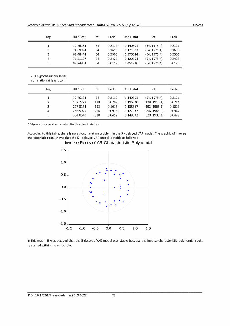
Research Journal of Business and Management – RJBM (2019), Vol.6(1). p.68-78 Ozyesil
_____________________________________________________________________________________________________ DOI: 10.17261/Pressacademia.2019.1022 78
Lag LRE* stat df Prob. Rao F-stat df Prob. 1 72.76184 64 0.2119 1.140601 (64, 1575.4) 0.2121
2 74.69924 64 0.1696 1.171683 (64, 1575.4) 0.1698
3 62.48444 64 0.5303 0.976344 (64, 1575.4) 0.5306
4 71.51107 64 0.2426 1.120554 (64, 1575.4) 0.2428
5 92.24804 64 0.0119 1.454936 (64, 1575.4) 0.0120
Null hypothesis: No serial correlation at lags 1 to h
Lag LRE* stat df Prob. Rao F-stat df Prob. 1 72.76184 64 0.2119 1.140601 (64, 1575.4) 0.2121
2 152.2228 128 0.0709 1.196820 (128, 1916.4) 0.0714
3 217.3174 192 0.1015 1.138667 (192, 1965.9) 0.1029 4 286.5945 256 0.0916 1.127037 (256, 1946.0) 0.0942
5 364.0540 320 0.0452 1.148332 (320, 1903.3) 0.0479
*Edgeworth expansion corrected likelihood ratio statistic.
According to this table, there is no autocorrelation problem in the 5 - delayed VAR model. The graphic of inverse characteristic roots shows that the 5 - delayed VAR model is stable as follows :
In this graph, it was decided that the 5 delayed VAR model was stable because the inverse characteristic polynomial roots
remained within the unit circle.
-1.5
-1.0
-0.5
0.0
0.5
1.0
1.5
-1.5 -1.0 -0.5 0.0 0.5 1.0 1.5
Inverse Roots of AR Characteristic Polynomial

Research Journal of Business and Management- RJBM (2019), Vol.6(1). p.79-87 Wei, Chiu, Wei, Wei
________________________________________________________________________________________________________ DOI: 10.17261/Pressacademia.2019.1023 79
IMPACT OF EIGHT DIMENSIONS ON THE BUSINESS OF SPECIALTY COFFEE SHOPS
DOI: 10.17261/Pressacademia.2019.1023
RJBM-V.6-ISS.1-2019(7)-p.79-87 Chiu-Chi Wei 1*, Chin-Hsin Chiu 2, Suz-Tsung Wei 3, Chiou-Shuei Wei 4 1* Chung Hua University, Industrial Management, 707, Sec.2, WuFu Rd., Hsinchu, Taiwan. [email protected] , ORCID: 0000-0002-9433-9114 2 Chung Hua University, Ph.D. Program of Technology Management, 707, Sec.2, WuFu Rd., Hsinchu, Taiwan. [email protected] , ORCID: 0000-0003-1842-5747 3 Fu Ren Catholic University, Business Administration, 505, Zhongzheng Rd., Xinzhuang Dist., New Taipei, Taiwan. [email protected] , ORCID: 0000-0002-1641-158X 4 Lunghwa University of Science and Technology, Industrial Management, 300, Wanshou Rd., Taoyuan, Taiwan. [email protected] , ORCID: 0000-0001-5925-7490
Date Received: November 20, 2018 Date Accepted: February 26, 2019
To cite this document Wei, C. C., Chiu, C. H., Wei, S. T., Wei, C. S. (2019). Impact of eight dimensions on the business of specialty coffee shops. Research Journal of Business and Management (RJBM), 6(1), p.79-87. Permemant link to this document: http://doi.org/10.17261/Pressacademia.2019.1023 Copyright: Published by PressAcademia and limited licenced re-use rights only.
ABSTRACT Purpose- The impacts of eight dimensions, including customer communication, customer relationship management, customer satisfaction,
customer loyalty, strategy management, customer trust, and service quality, on the business of specialty coffee shops were investigated,
Methodology- A questionnaire was designed to collect the data from 197 valid respondents; Structural Equation Modeling (SEM) was utilized to
analyze the data, and finally, Smart PLS was employed to validate the structural model.
Findings- Nine of the eleven hypothesized relationships were confirmed and supported, while two were not supported.
Conclusion- Results of this study can provide business owners of specialty coffee shops with valuable information and management implications.
Keywords: Brand image, strategy, customer relationship management, communication, customer loyalty, trust, service quality, customer
satisfaction, specialty coffee shop.
JEL Codes: C39, C61
1. INTRODUCTION
Coffee is one of the most popular beverages around the world, and is the second largest valuable traded commodity after petroleum (Murthy & Naidu, 2012). A lot of unique and specialty coffee shops have been opened in both rural and urban areas in Taiwan, and because of stiff competition, coffee shops have to perfect their service and quality to survive. Coffee business is dramatically growing globally, and statistics show that casual drink markets remain dominated by coffee shops. An overview of the recent decades on the global coffee sector reveals the largest growth (Kablan et al., 2017), and the figures show that the world coffee import data is increasing yearly, and that more people are enjoying specialty coffee globally (Han et al., 2018). Recently, specialty coffee shops have rapidly increased in various countries. In 2017, there was a 39.8% increase in the United Kingdom, 46% in America, 50% in Korea, and an astonishing growth of 61% in Taiwan. There is a projected 100% growth by 2020 (The Statistics Portal, 2018). Consequently, the competition in coffee shops promotes modernization of the coffee industry (Samoggia & Riedel, 2018).
Research Journal of Business and Management- RJBM (2019), Vol.6(1). p.79-87 Wei, Chiu, Wei, Wei
________________________________________________________________________________________________________ DOI: 10.17261/Pressacademia.2019.1023 80
Specialty coffee is quality coffee based beverages characterized by unique quality, incisive taste and personality to attractive customers. According to Shan et al. (2017), consumers greatly enjoy each coffee’s exclusive aroma and flavor (Zapata et al., 2018), and are willing to pay for high quality (Kang et al., 2012). Additionally, coffee has been recognized as a beverage with positive effects on human health (Kim, 2016). Previous research has also discovered that coffee improves social and personal well-being within emotionally taxing occupations (Stroebaek, 2013). Furthermore, products offering customer value help promote the economy, enhance health and increase happiness (Chen & Hu, 2010).
Based on the abovementioned background about specialty coffee industries, this study intends to explore the effects of eight dimensions on the business of specialty coffee shops, including customer communication, customer relationship management, customer satisfaction, customer loyalty, strategy management, customer trust, and service quality. This paper is composed of the following sections, the introduction, literature review, research method, research results and conclusion.
2. LITERATURE REVIEW
Coffee has enormous impact on globally lucrative beverage industries. Eight influential dimensions affecting the specialty coffee industry have been identified in different studies, including customer communication, customer relationship management, customer satisfaction, customer loyalty, strategy management, customer trust, service quality, and. brand image.
Customer communication is regarded as a complex construct that includes numerous apparatuses (Nadhar et al., 2017). Customer relationship marketing is helpful in eliciting customer value emanating from different origins, and thus contributes to successful strategic management (Lian & Yoong, 2017). Managers need to connect with and maintain relationships with their current and future customers to adequately fulfill the roles of communication and promotion (Kotler, 2000). The issue is usually not whether to communicate, but rather when, where and how to communicate to drive brand value (Hsieh et al., 2018). Customer Relationship Management (CRM) has changed the approaches of coffee shop interactions with current or potential consumers and influenced purchase behaviors by using customers’ historical data to improve business relationships with customers (Trainor et al., 2014). CRM programs intertwine script actions in communication pathways rather than promoting rich communication and facilitating emanating responses (Mitussis et al., 2006). It influences corporate culture, corporate identity, and employee’s needs (Triznova et al., 2015). It delivers superior customer value and satisfaction with the goal of improving business relationships with customers (Soltani & Navimipour, 2016). CRM mediates the relationship between service quality and customer satisfaction (Setiawan & Sayuti, 2017). Customer satisfaction can be categorized into two types: transaction-specific satisfaction and cumulative satisfaction (Kim, 2016). While customer satisfaction influences repurchase intentions and behaviors, however, Setiawan and Sayuti (2017) stated that satisfied customers cannot always be expected to return or to spread positive word-of-mouth because they may have actually been looking for something different (Qu et al., 2012). Lian and Yoong (2017) further showed that it is impossible to measure customer satisfaction measured without considering fulfillment. Customer loyalty is the aptitude of buyers to purchase specific products, services, and brands inside coffee shops (Han et al., 2018). Customer satisfaction and loyalty are concerned with the importance of a purchaser’s return, making of referrals, and provision of verbal advertisement (Verhoef, 2003). It points out customer satisfaction levels on customer loyalty (Tarak et al., 2014).
Strategic processes happen between businesses and their customers (Payne & Frow, 2005). These processes affect all interactions and create long-term value with customers (Bull, 2003). This concept also distinguishes between customers seeking economy and those holding onto expectations (Terho, 2015). Trust involves having customer needs or wants met. Trust emanates from the honesty and reliability of the opposite party in question (Verhoef, 2003). It remains fundamental, and affects customer confidence in the coffee shop (Young & Chiu, 2017). Service quality entails an assessment of expectations concerning service preference (Parasurman et al., 1985). Tangible service or satisfaction performance, a feeling that one party gives to the other, often results in actual ownership emotions (Setiawan & Sayuti, 2017). This kind of service influences the customer satisfaction perceived in coffee shops, customers’ loyalty and trust (Heri, 2017). Brand image is one of the important antecedents of buyer satisfaction and loyalty (Cailleba & Casteran, 2009; Ring et al., 2015). Discussing the positive relationship between branding and satisfaction Chin and Newsted (1999) stated that when buyers favor the brand image, colors, name, logo, personality styles, interesting design of the store, they will develop loyalty. Terho et al. (2015) emphasized the influence of brand image on customer loyalty. Branding increases satisfaction and loyalty in coffee industries (King, 2017). Founded upon the relationship of theory and purpose, researchers have shown that the above eight dimensions’ directly affect customers’ thoughts.

Research Journal of Business and Management- RJBM (2019), Vol.6(1). p.79-87 Wei, Chiu, Wei, Wei
________________________________________________________________________________________________________ DOI: 10.17261/Pressacademia.2019.1023 81
3. RESEARCH METHOD
Based on the literature review, we used an empirical study to explore the effects of brand image on various factors by analyzing the survey data to verify research hypotheses. To increase the validity of the research results of this study, a questionnaire was designed, pre-tested and modified. Structural equation modeling (SEM) was adopted for data analysis, and the validation of the structural model was achieved using Smart Partial Least Squares (Smart PLS) software.
The data collection was conducted for three months from January 1st to March 31st, 2018, in specialty coffee shops including “Professor Coffee Shop”, “Izzy Café”, and “Specially tailored Coffee Shop” in Taiwan. During the survey period, 220 completed questionnaires were collected, and after removing 23 incomplete questionnaires, a total sample of 197 valid responses was obtained. Among the valid responses, 97 of them were from males and the other 100 were from females. The age of participant was diverse, from younger than 18 to older than 65 years old, and the percentages were 2.8% for younger than 18, 15.2% for 18-24, 27.8% for 25-34, 27.0% for 35-44, 14.8% for 55-64, and 12.4% for above 65. As for educational background, 5.5% of respondents had not finished high school, 30.5% were high school graduates, 47.5% had college degrees and 16.5% had master’s or PhD degrees.
The questionnaire used the Likert 5-point scale from "1: strongly disagree" to "5: strongly agree", and Smart PLS was utilized to analyze the collected data. Smart PLS is a statistical technique of Structural Equation Model (SEM) using blocks, constructs and items to iteratively estimate factor loadings and path coefficients. Figure 1 illustrates the details.
Fıgure 1: Partial Least Square Model
The factor loading denotes the correlation between item and construct, while the path coefficient implies the level of influence between two constructs. PLS uses two stages to validate the research model, the first stage is to examine the outer model, including convergent validity and discriminant validity, in other words, to validate if the questionnaire can support the proposed construct. The second stage is to examine the inner model to validate if the proposed hypotheses can be accepted, and discover the degree of accuracy of the interpretation of the construct. The implementation of PLS can be described as below in Figure 3.
Figure 2: Example of PLS
X11
X12
X13
X21
X22
X23
X31
X32
X33
X41
X42
X43
block
Outer Model
(Formative model)
Outer Model
(Reflective model)
Inner Model
construct
item
X1
X2
X3
X4
X6
X7
X5 Y1
Y2
Y3
w1
w2
w3
w4
w5 w6
w7
p1
p2

Research Journal of Business and Management- RJBM (2019), Vol.6(1). p.79-87 Wei, Chiu, Wei, Wei
________________________________________________________________________________________________________ DOI: 10.17261/Pressacademia.2019.1023 82
Step 1: iteratively estimate the latent construct scores
A construct must be measured by several items, therefore, PLS uses the following methods to assign a number to the construct.
1.1 Apply the regression method to estimate the latent construct scores for constructs Y1, Y2 and Y3.
1.2 Use the above scores to estimate the path coefficients p1 and p2, using various scheme such as centroid scheme, factorial scheme, structural or path weighting scheme, and this study used path weighting scheme.
1.3 Use latent construct scores obtained in Step 1.1 and path coefficients obtained in Step 1.2 to adjust latent construct scores.
1.4 Re-estimate factor loading w1 to w7.
Step 2: Utilize ordinary least square method to finalize the estimation of factor loading and path coefficients; in other words, to converge the estimate to a certain value.
The results of PLS can be verified using two values, the composite reliability and R square. The value of composite reliability must be greater than 0.7 (Hair et al. 2010), and the value of R square must be larger than 0.33 for average significance and 0.67 for substantial significance (Chin 1998), denoting the degree that the independent variable can explain the dependent variables. A value of 1 implies 100 % and 0 implies 0%.
Based on the research objective and research method, this study developed the following hypotheses to be validated:
H1: Communication positively influences customer relationship management.
H2: Communication positively influences customer satisfaction.
H3: Customer loyalty positively influences brand image.
H4: Customer relationship management positively influences customer loyalty.
H5: Customer relationship management positively influences customer satisfaction.
H6: Customer relationship management positively influences strategy.
H7: Customer satisfaction positively influences customer loyalty.
H8: Customer satisfaction positively influences customer trust.
H9: Service quality positively influences customer satisfaction.
H10: Strategy positively influences brand image.
H11: Customer trust positively influences customer loyalty.
4. RESEARCH RESULTS
This section describes the results of this study, and the effects of brand image on the business of specialty coffee shops are discussed by validating the hypotheses related to the eight dimensions. Table 1 lists the results, and the composite reliability indexes obtained were 0.952 for brand image, 0.944 for communication, 0.936 for customer loyalty, 0.957 for customer relationship management, 0.921 for customer satisfaction, 0.942 for service quality, 0.957 for strategy management, and 0.969 for customer trust respectively. The composite reliability must be greater than 0.8; therefore, it can be seen from the values that all of them are reliable (Hair et al., 2014).
The average variance extracted (AVE) for each factor are shown in Table 1. It is obvious that all values are far above 0.5 and were found to have convergent validity. The values of R square for each factor obtained were 0.665 for brand image, 0.664 for communication, 0.667 for customer loyalty, 0.573 for customer relationship management, 0.641 for customer satisfaction, 0.664 for service quality, 1.000 for strategy, and 0.521 for trust. It is apparent that all values are larger than the average level of 0.33, and slightly below the substantial level of 0.67. The above data indicated that the convergent validity and discriminant validity of the results were confirmed. Furthermore, the internal consistency or composite reliability can be verified using the composite alpha value, and it is obvious that all alpha values in Table 1 are more than 0.7 (Hair et al. 1998), indicating that a high degree of internal consistency was found in this study.

Research Journal of Business and Management- RJBM (2019), Vol.6(1). p.79-87 Wei, Chiu, Wei, Wei
________________________________________________________________________________________________________ DOI: 10.17261/Pressacademia.2019.1023 83
Table 1: Reliability and Validity
Dimensions R Square R Square Adjusted α Composite Reliability AVE
Brand Image 0.665 0.661 0.940 0.952 0.768
Communication 0.664 0.660 0.925 0.944 0.770
Customer Loyalty 0.667 0.662 0.908 0.936 0.784
Customer Relationship Management 0.573 0.570 0.940 0.957 0.848
Customer Satisfaction 0.641 0.636 0.893 0.921 0.700
Service Quality 0.664 0.660 0.922 0.942 0.764
Strategy 1.000 1.000 0.940 0.957 0.848
Trust 0.521 0.518 0.961 0.969 0.864
4.1 Pearson’s Correlation Coefficients
The Pearson’s correlation coefficient is used to measure the statistical relationship between dimensions. It is a well-known method for measuring the correlation between variables of interest because it is based on the method of covariance. It provides information about the magnitude of the correlation and the direction of the relationship. Two variables are perfectly correlated when the Pearson’s correlation coefficient is 1; highly correlated variables fall between 0.7 and 0.99; moderately correlated variables range between 0.4 and 0.69; modestly correlated variables fall between 0.1 and 0.39; weakly correlated variables are between 0.01 and 0.09; and 0 indicates no correlation at all. It can be seen from Table 2 that brand image is highly correlated with communication, customer loyalty, CRM, service quality, strategy and trust, because values of correlation coefficients are all greater than 0.7; similarly, communication is highly correlated with brand image, CRM, customer satisfaction, service quality strategy and trust; customer loyalty is highly correlated with brand image, CRM, strategy and trust; CRM is highly correlated with brand image, communication, customer loyalty, service quality, strategy and trust; customer satisfaction is highly correlated with communication, service quality and trust; service quality is highly correlated with brand image, communication, CRM, customer satisfaction, strategy and trust; strategy is highly correlated with brand image, communication, customer loyalty, CRM, service quality and trust; trust is highly correlated with brand image, communication, customer loyalty, CRM, customer satisfaction, service quality and strategy. Furthermore, strategy is perfectly correlated with CRM. Table 2 lists the details.
Table 2: Pearson Correlation Coefficients
BI CO CL CRM CS SQ S T
Brand image 1.000
Communication 0.717 1.000
Customer loyalty 0.778 0.666 1.000
CRM 0.772 0.757 0.807 1.000
Customer satisfaction 0.679 0.776 0.631 0.699 1.000
Service quality 0.727 0.875 0.661 0.762 0.751 1.000
Strategy 0.772 0.756 0.807 1.000 0.698 0.762 1.000
Trust 0.719 0.764 0.747 0.856 0.722 0.813 0.856 1.000

Research Journal of Business and Management- RJBM (2019), Vol.6(1). p.79-87 Wei, Chiu, Wei, Wei
________________________________________________________________________________________________________ DOI: 10.17261/Pressacademia.2019.1023 84
4.2. Structural Model
A structural model is utilized to capture the linear regression effects of endogenous constructs upon one another, and it has the ability to specify the pattern of relationships among the constructs (Hair et al., 1998; Leohlin, 2998). A structural model was
evaluated using three criteria: (1) path coefficients ( value), (2) path significant (p value), and (3) variance explain (R2 value). The bootstrap re-sampling method was used to test the statistical significance of each path coefficient. 500 iterations using randomly selected sub-samples were performed to estimate the hypothesized relationships. Figure 4 illustrates the structural model. All statistical tests were assessed at a 5% level of significance using two-tailed t-tests.
Figure 3: Structural Model
The results of the full model indicate that 57.3% of the variance in customer relationship management was explained by the
model; 66.4% of the variance in communication was explained by the model; 66.4% of the variance in service quality was
explained by the model; 64.1% of the variance in customer satisfaction was explained by the model; 52.1% of the variance in
trust was explained by the model; 100.0% of the variance in strategy was explained by the model; 66.7% of the variance in
customer loyalty was explained by the model; 66.5% of the variance in brand image was explained by the model. The evaluation
criteria for validating the hypothesis was the use of t-values for each path loading, and the cut-off criteria was a t-value larger or
equal to 1.645 for an alpha value of 0.05 (Hair et al. 2006).
Hypothesis H1 states that communication positively influences customer relationship management. Figure 4 shows that the
hypothesized path for H1 was positive and significant (=0.757, p<0.05), thus hypothesis H1 was supported.
Hypothesis H2 states that communication positively influences customer satisfaction. The hypothesized path for H2 was positive
and significant (=0.427, p<0.05), thus hypothesis H2 was supported.
Hypothesis H3 states that customer loyalty positively influences brand image. The hypothesized path for H3 was positive and
significant (=0.442, p<0.05), thus hypothesis H3 was supported.
Hypothesis H4 states that customer relationship management positively influences customer loyalty. The hypothesized path for
H4 was positive and significant (=0.601, p<0.05), thus hypothesis H4 was supported.
0.664
0.664

Research Journal of Business and Management- RJBM (2019), Vol.6(1). p.79-87 Wei, Chiu, Wei, Wei
________________________________________________________________________________________________________ DOI: 10.17261/Pressacademia.2019.1023 85
Hypothesis H5 states that customer relationship management positively influences customer satisfaction. The hypothesized
path for H5 was positive and significant (=0.210, p<0.05), thus hypothesis H5 was supported.
Hypothesis H6 states that customer relationship management positively influences strategy. The hypothesized path for H6 was
positive and significant (=1.000, p<0.05), thus hypothesis H6 was supported.
Hypothesis H7 states that customer satisfaction positively influences customer loyalty. The hypothesized path for H7 was not
significant (=0.089, p>0.1), thus hypothesis H7 was not supported.
Hypothesis H8 states that customer satisfaction positively influences customer trust. The hypothesized path for H8 was positive
and significant (=0.217, p<0.05), thus hypothesis H8 was supported.
Hypothesis H9 states that service quality positively influences customer satisfaction. The hypothesized path for H9 was positive
and significant (=0.722, p<0.05), thus hypothesis H9 was supported.
Hypothesis H10 states that strategy positively influences brand image. The hypothesized path for H10 was positive and
significant (=0.415, p<0.05), thus hypothesis H10 was supported.
Hypothesis H11 states that customer trust positively influences customer loyalty. The hypothesized path for H11 was not
significant (=0.168, p>0.1), thus hypothesis H11 was not supported.
5. CONCLUSION
This study explored the effects of eight dimensions on the business of specialty coffee shops, including customer communication, customer relationship management, customer satisfaction, customer loyalty, strategy management, customer trust, and service quality. An empirical study was applied to collect data using a questionnaire survey conducted in Taiwan, and structural equation modeling was adopted to analyze data, while Smart PLS was used to validate the structural model. Results of the research indicated that the all of the Cronbach’s alpha values tracking the internal consistency of the scale exceeded 0.7; all factor loadings are far above the acceptable level of 0.5; all composite reliability values for each construct are greater than 0.7; all values of average variance extracted for each construct are also larger than 0.5. Therefore, convergent validity and discriminative validity of this study were confirmed. Nine of the eleven hypothesized relationships were supported, except for the relationships between customer trust and customer loyalty, and between customer satisfaction and customer loyalty. This may be attributed to the fact that customer trust is just the prerequisite for visiting a specialty coffee shop, and not enough to induce customer loyalty. On the other hand, the reason that customer satisfaction did not contribute to customer loyalty may be due to the fact that customers visiting a specialty coffee shop may easily be attracted to other coffee shops providing new flavors and fashionable atmospheres. This would conform to the research results from previous studies. However, the conclusion of this study could be further explored using individual in-depth interviews to dive into the internal cognition of customers.
REFERENCES
Bull, C. M. (2003). Strategic issues in customer relationship management (CRM) implementation. Business Process Management Journal, vol. 9, no. 5, pp.592-602.
Cailleba, P., Casteran, H. (2009). A quantitative study on the fair trade coffee consumer. The Journal of Applied Business Research, vol. 25, no. 6, pp.31-46.
Chen, P. T., Hu, H. H. (2010). How determinant attributes of service quality influence customer‐perceived value: An empirical investigation of the Australian coffee outlet industry. International Journal of Contemporary Hospitality Management, vol. 22, no. 4, pp.535-551.
Chin, W., Newsted, P. (1999). Structural Equation Modeling Analysis with Small Samples Using Partial Least Squares. In R. H. Hoyle (Ed.), Statistical Strategies for Small Sample Research. Thousand Oaks: Sage Publications. pp.307-341.
Hair, J., Hult, G., Ringle, C., Sarstedt, M. (2014). A primer on partial least squares structural equation modeling (PLS-SEM). SAGE Publications.
Han, H., Nguyen, H. N., Song, H., Chua, B. L., Lee, S., Kim, W. (2018). Drivers of brand loyalty in the chain coffee shop industry. International Journal of Hospitality Management, vol. 72, pp.86-97.

Research Journal of Business and Management- RJBM (2019), Vol.6(1). p.79-87 Wei, Chiu, Wei, Wei
________________________________________________________________________________________________________ DOI: 10.17261/Pressacademia.2019.1023 86
Heri, H. (2017). Analysis the effect of service quality, customers value, customer satisfaction and customer trust on corporate image. Journal of Business and Management, vol. 19, no. 6, pp.38-46.
Hsieh, C. M., Chen, T. P., Hsieh, C. J., Tsai, B. K. (2018). Moderating effect of membership status on the quality-value-loyalty chain at museums. Social Behavior and Personality: an international journal, vol. 46, no. 1, pp.107-126.
Hulland, J. (1999). Use of partial least squares (PLS) in strategic management research: a review of four recent studies. Strategic Management Journal. vol. 20, no. 2, pp.195-204.
Kablan, S., Ftiti, Z., Guesmi, K. (2017). Commodity price cycles and financial pressures in African commodities exporters. Emerging Markets Review, vol. 30(C), pp.215-231.
Kang, J., Tang, L., Lee, J. Y., Bosselman, R. H. (2012). Understanding customer behavior in name-brand Korean coffee shops: The role of self-congruity and functional congruity. International Journal of Hospitality Management, vol. 31, pp.809-818.
Kim, S. E., Lee, S. M., Kim, K. O. (2016). Consumer acceptability of coffee as affected by situational conditions and involvement. Food Quality and Preference, vol. 52, pp.124-132.
King, C. (2017). Brand management – standing out from the crowd: A review and research agenda for hospitality management. International Journal of Contemporary Hospitality Management, vol. 29, no. 1, pp.115-140.
Kotler, P. (2000). Marketing management: analysis, planning, implementation and control (seventh ed). New Jersey: Prentice Hall.
Lian, S. B. Yoong, L. C. (2017). The effectiveness of strategic relationship marketing: exploring relationship quality towards customer loyalty. International Business Research, vol. 10, no. 12, pp.159-166.
Likert, R. (1932). A technique for the measurement of attitudes. New York: Archives of Psychology.
Murthy, P. S., Naidu, M. (2012). Sustainable management of coffee industry by-products and value addition-A review. Resources Conservation and Recycling, vol. 66, pp.45-58.
Mitussis, D., O’Malley, L., Patterson, M. (2006). Mapping the re-engagement of CRM with relationship marketing. European Journal of Marketing, vol. 40, no. 5, pp.572-589.
Nadhar, M., Tawe, A., Parawansa, D. (2017). The effect of work motivation and entrepreneurship orientation on business performance through entrepreneurial commitments of coffee shops in Makassar. International Review of Management and Marketing, vol. 7, no. 1, pp.470-474.
Ou, W. M., Shih, C. M., Chen, C. Y., Tseng, C. W. (2012). Effects of ethical sales behaviour, expertise, corporate reputation, and performance on relationship quality and loyalty. The Service Industries Journal, vol. 32, no. 5, pp.773-787.
Parasurman, A., Zeithaml, A., Berry, L. (1985). A conceptual model of service quality and its implications for future research. Journal of Marketing, vol. 49, no. 4, pp.41-50.
Payne, A., Frow. P. (2005). A strategic framework for customer relationship management. Journal of Marketing, vol. 69, pp. 167-176.
Ringle, C., Wende, S., Beck, J. (2015). SmartPLS 3. Boenningstedt: SmartPLS GmbH.
Samoggia, A., Riedel, B. (2018). Coffee consumption and purchasing behavior review: Insights for further research. Appetite, vol. 129, no. 1, pp.70-81.
Setiawan, H., Sayuti, A. (2017). Effects of service quality, customer trust and corporate image on customer satisfaction and loyalty: An assessment of travel agencies customer in South Sumatra Indonesia. Journal of Business and Management, vol. 19, no. 5, pp.31-40.
Soltani, Z., Navimipour, N. (2016). Customer relationship management mechanisms: A systematic review of the state of the art literature and recommendations for future research. Computer in Human Behavior, vol. 61, pp. 667-688.
Stroebaek, P. S. (2013). Let’s have a cup of coffee! Coffee and coping communities at work. Symbolic Interaction, vol. 36, no. 4, pp.381-397.
Tarak, P. (2014). Customer communication dimension of marketing mix- a review of gap between mutual fund investors’ expectation and experience. Scholars Journal of Economics Business and Management, vol. 1, no. 5, pp.197-202.
Terho, H., Eggert, A., Haas, A., Ulaga, W. (2015). How sales strategy translates into performance: The role of salesperson customer orientation and value-based selling. Industrial Marketing Management, vol.45, pp.12-21.
The Statistics Portal. 2018, https://www.statista.com/statistics/270091/coffee-house- chains-ranked-by-revenue/
Trainor, K., Andzulis, J., Rapp, A., Agnihotri, R. (2014). Social media technology usage and customer relationship performance: A capabilities-based examination of social CRM. Journal of Business Research, vol. 67, no. 6, pp. 1201-1208.

Research Journal of Business and Management- RJBM (2019), Vol.6(1). p.79-87 Wei, Chiu, Wei, Wei
________________________________________________________________________________________________________ DOI: 10.17261/Pressacademia.2019.1023 87
Triznova, M., Mat’ova, H., Dvoracek, J., Sadek, S. (2015). Customer relationship management based on employees and corporate culture. Procedia Economics and Finance, vol. 26, pp. 953-959.
Verhoef, P. C. (2003). Understanding the effect of customer relationship management efforts on customer retention and customer share development. Journal of Marketing, vol. 67, pp.30-45.
Young, L. J., Chiu, C. H. (2017). Is it feasible to use service quality, trust, and commitment management to determine customers’ loyalty?. Transylvanian Review, vol. 20, pp. 5609-5619.
Zapata, J., Londoño, V., Naranjo, M., Osorio, J., Lopez, C., Quintero, M. (2018). Characterization of aroma compounds present in an industrial recovery concentrate of coffee flavor. CyTA - Journal of Food, vol. 16, no. 1, pp.367-372.