research - minnesota department of transportation · this report represents the results of research...
TRANSCRIPT

2005-06 Final Report
Moisture Retention Characteristics of Base and Sub-base Materials
Research

Technical Report Documentation Page 1. Report No. 2. 3. Recipients Accession No.
MN/RC – 2005-06 4. Title and Subtitle 5. Report Date
December 2004 6.
Moisture Retention Characteristics of Base and Sub-base Materials
7. Author(s) 8. Performing Organization Report No.
Satish Gupta, Amanjot Singh Andry Ranaivoson
9. Performing Organization Name and Address 10. Project/Task/Work Unit No.
11. Contract (C) or Grant (G) No.
University of Minnesota Department of Soil, Water, & Climate 1991 Upper Buford Circle St. Paul, MN 55108
(c) 81655 (wo) 49
12. Sponsoring Organization Name and Address 13. Type of Report and Period Covered
Final Report 14. Sponsoring Agency Code
Minnesota Department of Transportation Research Services Section 395 John Ireland Boulevard Mail Stop 330 St. Paul, Minnesota 55155
15. Supplementary Notes
http://www.lrrb.org/PDF/200506.pdf 16. Abstract (Limit: 200 words)
Soil water retention refers to the relationship between the amount of soil water and the energy with which it is held. This relationship is important for characterizing water movement through granular materials. In this project, we generated soil moisture retention data of 18 non-recycled and 7 recycled materials used in pavement construction. The results showed that water retention of non-recycled materials was nearly similar. The major differences among the curves were in the inflection points (air entry values) and in the water contents either near saturation or at 15,300 cm of suction. Using this database, we also developed Pedo-transfer functions that can predict (1) water retention or (2) the parameters of functions that describe water retention from easily measurable properties of the pavement materials. Water retention of concrete with and without shingles was only slightly different. This is partially because shingle chips imbedded in the concrete were large. Traditionally, the influence of matric suction has not been directly considered in pavement design. The water retention data in this report will be helpful in developing resistance factors for Minnesota Flexible Pavement Design Program either through physical modeling or through statistical relationships between design criteria and the water contents.
17. Document Analysis/Descriptors 18.Availability Statement
Soil water retention Pavement construction Pedo-transfer functions
Concrete Base materials Sub-base materials
No restrictions. Document available from: National Technical Information Services, Springfield, Virginia 22161
19. Security Class (this report) 20. Security Class (this page) 21. No. of Pages 22. Price
Unclassified Unclassified 112

Moisture Retention Characteristics of Base and Sub-base Materials
Final Report
Prepared by: Satish Gupta
Amanjot Singh Andry Ranaivoson
Department of Soil, Water, & Climate
University of Minnesota
December 2004
Published by: Minnesota Department of Transportation
Research Services Section 305 John Ireland Boulevard, MS 330
St. Paul, MN 55155
This report represents the results of research conducted by the authors and does not necessarily represent the views or policies of the Minnesota Department of Transportation and/or the Center for Transportation Studies. This report does not contain a standard or specified technique.

TABLE OF CONTENTS
Chapter 1 INTRODUCTION ...................................................................................................... 1
Chapter 2 OBJECTIVES .............................................................................................................. 3
Chapter 3 SCOPE .......................................................................................................................... 4
Chapter 4 METHODOLOGY ...................................................................................................... 5
PARTICLE SIZE DISTRIBUTION AND CHEMICAL AND MINERALOGICAL......................... 5 WATER RETENTION............................................................................................................................. 5 DEVELOPMENT OF PEDO-TRANSFER FUNCTIONS .................................................................. 6 ESTIMATION OF VAN GENUCHTEN, BROOKS- COREY.......................................................... 6 STATISTICAL A NALYSIS................................................................................................................... 7
Chapter 5 RESULTS ..................................................................................................................... 8 PARTICLE SIZE DISTRIBUTION AND CHEMICAL AND MINERALOGICAL PROPERTIES.8 WATER RETENTION CURVES (DESORPTION)............................................................................. 8 PEDO-TRANSFER FUNCTION MODEL ........................................................................................... 9 PEDO-TRANSFER FUNCTION MODEL VALIDATION ................................................................ 9 VAN GENUCHTEN, BROOK-COREY, AND FREDLUND-XING PARAMETERS.................... 9 PREDICTIONS FROM EXISTING MOD ELS .................................................................................. 11 WETTING CURVES ............................................................................................................................. 12 WATER RETENTION OF RECYCLED MATERIALS ................................................................... 12
Chapter 6 DISCUSSION ............................................................................................................. 13
Chapter 7 EXPECTED BENEFITS ........................................................................................... 14
References...................................................................................................................................... 15
Appendix A.............................................................................................................................A- 1 Appendix B.............................................................................................................................B-1 Appendix C.............................................................................................................................C-1 Appendix D.............................................................................................................................D-1 Appendix E.............................................................................................................................E-1 Appendix F..............................................................................................................................F-1 Appendix G.............................................................................................................................G-1 Appendix H.............................................................................................................................H-1

LIST OF TABLES Table 1. ..................................................................................................................................... 17 Table 2.. .................................................................................................................................... 18 Table 3. ..................................................................................................................................... 18 Table 4.. .................................................................................................................................... 19 Table 5.. .................................................................................................................................... 19 Table 6.. .................................................................................................................................... 20 Table 7.. .................................................................................................................................... 20 Table 8.. .................................................................................................................................... 21 Table 9. . ................................................................................................................................... 22 Table 10. ................................................................................................................................... 22 Table 11. ................................................................................................................................... 23 Table 12.. .................................................................................................................................. 23 Table 13. ................................................................................................................................... 24 Table 14. ................................................................................................................................... 24 Table 15.. .................................................................................................................................. 24 Table 16. ................................................................................................................................... 25 Table 17. ................................................................................................................................... 25

LIST OF FIGURES Figure 1..................................................................................................................................... 26 Figure 2..................................................................................................................................... 27 Figure 3..................................................................................................................................... 28 Figure 4..................................................................................................................................... 29 Figure 5..................................................................................................................................... 30 Figure 6..................................................................................................................................... 31 Figure 7..................................................................................................................................... 32 Figure 8..................................................................................................................................... 33 Figure 9..................................................................................................................................... 34 Figure 10................................................................................................................................... 35 Figure 11................................................................................................................................... 36 Figure 12................................................................................................................................... 37 Figure 13................................................................................................................................... 38 Figure 14................................................................................................................................... 39 Figure 15................................................................................................................................... 40 Figure 16................................................................................................................................... 41 Figure 17................................................................................................................................... 42 Figure 18................................................................................................................................... 43 Figure 19................................................................................................................................... 44 Figure 20................................................................................................................................... 45 Figure 21................................................................................................................................... 46 Figure 22................................................................................................................................... 47

EXECUTIVE SUMMARY
Soil water retention refers to the relationship between the amount of soil water and the energy with which it is held. This relationship is not only an indicator of the pore size distribution but also the volume occupied by various pore classes. The relationship is important for characterizing the rate at which water moves through a granular material under both saturated and unsaturated conditions. Important consequences of this relationship are the amount of drainage that occurs through soils, how deep the frost penetrates, and how strength properties vary seasonally. Although there is substantial information in the literature on soil water retention characteristics, most of this information is for relatively loose agricultural soils. The goal of the project was to generate soil moisture retention data for compacted aggregate base, sub-base, and subgrade materials used in pavement construction. Since there is an increasing emphasis on the use of recycled materials in roadbed preparation, the secondary goal of this project was to characterize the water retention properties of aggregate base materials that contained recycled material. In this study, we characterized the physical and chemical properties and wetting and drying water retention characteristics of 18 samples of non- recycled base and sub-base materials. These samples included thirteen samples of Select Granular (SG), one sample of class-4 (CL-4), four samples of class-5 (CL-5). In addition, we characterized the above properties in 7 recycled materials used in roadbed construction. These materials include one sample each of concrete, crushed concrete, crushed concrete with shingles, and 4 samples of bottom ash. The results showed that most base and sub-base materials used for roadbed construction in Minnesota are nearly similar in terms of traditional sand, silt, and clay contents. In general, drying curves of these materials were nearly similar (within a narrow range of water contents). The main differences among these curves were in the inflection points (air entry values) and in the water contents either near saturation or at 15,300 cm of suction. This is expected considering that particle size distribution of most samples were nearly similar. In this study, we also developed Pedo-transfer function models that predict water retention properties of roadbed materials from easily measurable properties such sand % and dry bulk density or the water retention function parameters of van Genuchten, Brook and Corey, Fredlund and Xing equations from particle size distribution, percent particles passing #200, D10, D60, or the grading numbers. We also tested the empirical and physico-empirical models in the literature for predicting water retention of roadbed materials. In general, these models did not predict well the water retention properties of roadbed materials because of high densities (up to 1.95 Mg m-3) or low clay content. There was only a slight difference in water retention of concrete with and without shingles. This is partially because shingle chips imbedded in the concrete were large and thus did not alter the properties of the concrete. However, orientation of imbedded shingles can have significant effect on pathways for water flow in base and sub-base materials. The influence of matric suction has traditionally not been directly considered in pavement design. The water retention data in this report will be helpful in developing resistance factors for Minnesota Flexible Pavement Design Program (MnPAVE) either through physical modeling or through statistical relationships between design criteria and the water contents.

1
Chapter 1: INTRODUCTION
Soil water retention refers to the relationship between the amount water in soil and the energy with which it is held. This relationship is not only an indicator of the pore size distribution but also the volume occupied by various pore classes. The relationship is important for characterizing the rate at which water moves through a granular material and its strength and stiffness under both saturated and unsaturated conditions. Important consequences of this relationship are the amount of drainage that occurs through soils, how deep the frost penetrates, and how strength properties vary seasonally. Since soil particle packing leads to formation of many different size pore necks and pore bodies, water retention of granular material also varies depending upon the size distribution of the granular material, the shape of the particles, and how they are packed. Furthermore, since different pore neck sizes and pore bodies are joined together in a sequence, this leads to different soil water retention characteristics depending on whether soil is wetting or drying. Before 1979, there was substantial information in the literature on water retention characteristics of different soils but there was no easy way to predict these properties for other unknown soils and soil materials. Gupta and Larson (1979) were among the first who developed Pedo-transfer functions for predicting water retention characteristics of soils. Since that time, there have been significant efforts toward building of soil hydraulic properties databases as well as in improving Pedo-transfer functions. Notable among those are the works of Rawls and Brakensiek (1981) and Rawls et al. (1982). Since the mid 1960's there have been other efforts made to develop new methods of predicting hydraulic properties based on material characterization (Mualem, 1976; Arya and Paris, 1981) and thus, better representation of the hydraulic functions (Brook and Corey, 1964; Campbell, 1974; and van Genuchten, 1980). In 1989, an international conference was held to summarize the existing knowledge on soil water retention characteristics and to present method of estimating these properties for unsaturated soils (van Genuchten et al., 1992). One product of this conference was a collection of all databases that were available in the literature. Since that time, these databases have grown and are now routinely used in many modeling efforts. In 1997, a second international conference was held on characterization and measurement of the hydraulic properties of unsaturated porous media” (van Genuchten et al., 1999). In this conference, besides improving the existing methodologies for determining hydraulic properties and Pedo-transfer functions, research was also summarized on additional artifacts in water flow such as preferential flow and water retention characteristics of multi-phase systems. Although there is a large amount of data available on soil water retention characteristics a limitation of existing databases is that moisture characterization is for relatively loose agricultural soils at or below natural field bulk densities. Water retention data for low clay highly compacted soils, as is the case for pavement base and sub-base, is limited. Also, there is no single transfer function model available for predicting water retention characteristics of aggregate base or granular subgrade materials from easily measurable soil properties. Most numerical simulations of water flow and drainage under pavements in the literature have been made with water retention characteristics estimated using loose agricultural soils databases

2
(Roberson et al., 2004). However, there is no confirmation of predictions relative to the measured values. Minnesota Department of Transportation (Mn/DOT) is currently using a relatively small database (SoilVision®) which includes the work by Fredlund and Xing (1994) in the field of geotechnical engineering. This project was started with the idea of generating soil moisture retention database for compacted aggregate base, granular, sub-base and subgrade soils typically used in pavement construction and then using this database to develop methods for predicting these properties for unknown materials. The long-term goal is to incorporate this database in the Soil Vision software so that soil water retention properties for unbound pavement materials can be generated from easily measurable properties such as particle size distribution. Since there is an increasing use of recycled materials in roadbed construction, there is also a potential for change in water retention properties and thus soil water flow when recycled materials are mixed with aggregate base and sub-base materials. Alteratio n in the water retention properties of the materials due to mixing of recycled materials may be due to differences in physical properties such as grain size and shape (small chips in case of shingles) or due to chemical properties such as wettability (in case of shredded tires and shingles) or due to cementation (with ash fly). Specifically, the goal of this project was to characterize water retention characteristics of aggregate base and sub-base materials during both drying and wetting cycles and then develop procedures that can be used to predict these properties from relatively simple measurements such as particle size distribution and packing density.

3
Chapter 2: OBJECTIVES Specific objectives of the study were:
• Develop wetting and drying water retention charac teristics of aggregate base, sub-base, and subgrade materials including select granular materials used in roadbed construction.
• Develop best-fit parameters of Brooks and Corey (1966), Van Genuchten (1980), and Fredlund and Xing (1994) functions that describe water retention characteristics.
• Quantify the gradation of these base materials in terms of parameters such as particle size distribution, % passing #200, D10, D60, or grading numbers.
• Develop Pedo-transfer functions of water retention at a given suction to material gradation properties.
• Develop regression relationships between Van Genuchten, Brook and Corey and Fredlund and Xing function parameters to material gradation properties.
• Run moisture retention characteristics on 5-10 aggregate base materials that contain recycled material.
• Identify the impact of recycled material on hydraulic properties.

4
Chapter 3: SCOPE The study characterized water retention characteristics of 18 aggregate base and sub-base materials that bracket the extremes of gradation bands. These samples were classified according to Mn/DOT specifications and include thirteen samples of Select Granular (SG), one sample of class-4 (CL-4), four samples of class-5 (CL-5). These samples include aggregates that are believed to provide good pavement drainage. Six of the thirteen select granular samples were also used in another study by the Civil Engineering department at the University of Minnesota to characterize their resilient modulus (Davich et al., 2004). Samples of these specified gradations were generated by Mn/DOT laboratory through mixing or were collected from field sites by the Mn/DOT personnel. The study also characterized the water retention characteristics of 7 recycled materials used in roadbed construction. These materials were selected in consultation with the Recycled Materials Resource Center at the University of New Hampshire. These materials include one sample each of concrete, crushed concrete, crushed concrete with shingles, and 4 samples of bottom ash.

5
Chapter 4: METHODOLOGY
Particle Size Distribution and Chemical and Mineralogical Properties The particle size distribution of the roadbed materials was estimated using dry sieve apparatus for particles sizes >0.075 inches (0.19 mm) and Horiba LA-910 Laser Analyzer for finer particles. The gradation was done at the Mn/DOT Soil Laboratory. This particle size analysis was used to calculate the grading number (GN) of each sample.
100075.0425.00.275.45.91925
(%)mmmmmmmmmmmmmm
GN++++++
= Eq. [1]
where all numbers are in percent passing a given sieve size. Maximum value of GN is 7.0 and represents the extremely fine gradation whereas minimum value of GN is 0.0 and represents the very coarse gradation. Grading number for both the coarse and the fine fractions were calculated. Coarse grading number (CGN) accounted for particles between 4.75 to 25 mm diameter whereas fine grading number (FGN) accounted for particles between 0.075 and 2.0 mm diameter particles (Table 1). Kremer and Dai (2004) showed that strength measurements with the Dynamic Cone Penetrometer were related to grading numbers. Base and sub-base materials were also tested for dissolved heavy metals and other basic elements. The procedure involved mixing soil and water in 1:10 ratio, shaking the suspension for 24 hours and then centrifuging the suspension for 20 minutes at 6000 rpm. The dissolved chemicals were analyzed in the supernatant on the Inductive Coupled Plasma (ICP). The Soil Geomorphology Laboratory at the University of Nebraska analyzed the samples for clay mineralogy. The procedure involved separating the clay particles and running the x-ray diffraction of clay particles mounted on a glass slide. Peaks in diffraction patterns are then used to separate out various clay minerals present in the sample. Water Retention Drying and wetting water retention characteristics were measured on all samples. At a given suction, the amount of water held in soil during drying is greater than that during wetting. In other words, it takes more force to desorb than to sorb water from a soil material at a given water content. This hysteretic effect is mainly due to elliptical nature of the soil pores (Gupta and Wang, 2002). The procedure for water retention curves involved preparing the soil sample to optimum water content identified by the Standard Proctor test and then packing the soil in metal cores to a maximum density also identified in the Standard Proctor test. Both optimum water content and density values were provided by Mn/DOT (Table 1). For drying curves, soil cores were saturated and then desorbed by applying a given air pressure in a pressure chamber. The soil drains the excess water over and above its retention capacity at that pressure. Once equilibrium was reached, the soil was subjected to the next air pressure and the outflow was measured. This process was repeated until the air pressure equivalent to the air entry value of

6
the ceramic plate was reached. Finally, the soil core was taken out of the pressure chamber, weighed, and then oven dried at 105 oC. Water content at a given pressure was then calculated from the final water content of the soil core and the volume of outflow between pressure steps. Details of the procedure are given in Appendix A1 and A2. Drying curves for the roadbed material covered a pressure head range of 10.2 cm to 15,300 cm H2O. Several different apparatuses were used to cover the full range:
• Tempe cell apparatus: pressure range from 10.2 to 1,020 cm H2O, • 5-bar pressure plate apparatus: pressure range from 102 to 3,060 cm H2O, • 15-bar pressure plate apparatus: pressure range from 1,020 to 15,300 cm H2O.
The pressure ranges overlapped and thus helped verify the accuracy of the results obtained from three different soil cores in three different pressure apparatuses. Sorption curves were measured in a Tempe cell and covered the pressure range from 10.2 to 1020 cm H2O head. The procedures for the wetting curve involved subjecting the soil core packed at the optimum water content to an air pressure corresponding to the suction desired. This was done while the soil core was in contact with a reservoir of water that is at atmospheric pressure. Atmospheric pressure at the base of the ceramic plate was maintained with a Marriott bottle set-up. The drop in water level in the Marriott bottle then corresponds to the volume of water that is adsorbed by the soil at a given air pressure. Details of the procedures for wetting curve are also given in the Appendix A3. Development of Pedo-transfer functions Drying soil water retention curves were used to develop Pedo-transfer functions. The procedure involved running stepwise regression of water retention at a given suction to easily measurable soil properties such as sand, silt, and clay contents, and the bulk density. Multiple regressions were done using the SAS (SAS, 2004) or SYSTAT version 6.0 (1996) statistical package. Estimation of van Genuchten, Brooks-Corey, and Fredlund-Xing Parameters Analytical formulations have been proposed to describe the water retention of soil materials over the whole suction range. Two of the well-known relationships are by van Genuchten (1980) and Brooks and Corey (1966). van Genuchten parameters (Eq. [2]) were calculated using the RETC (van Genuchten et al., 1980) program.
( ) ( )[ ] mnhh−
−+=Θ α1 Eq. [2]
( ) ( )2
15.0 11
Θ−Θ=
m
msKK θθ
Eq. [3]

7
rs
r
θθθθ
−−=Θ
Eq. [4]
where h is matric potential (cm), α is inverse of the air-entry value, m and n are constants that describe the shape of the water retention curve (m=1-1/n), K(θs) is saturated hydraulic conductivity, Θ is the relative water content, θs is the saturated water content, and θr is the residual water content. Brooks and Corey formulations can be described as:
cn
a
hh
=Θ Eq. [5]
cn
sKK 23)()( +Θ= θθ Eq. [6] where ha is the air entry suction and nc is the pore size distribution index. Brooks and Corey parameters were obtained by fitting Eq. [5] to the measured data in a Soil Vision program. Fredlund and Xing (1994) presented a more generalized equation (Eq. [7]) for describing the water retention characteristic of the soil materials.
( )[ ]
mf
nf
fr
rs
a
hh
hh
=
+
+
−=
1expln
110
1ln
1ln
16
θθ
Eq. [7]
where hr is the suction at which residual water content occurs, af is a soil parameter (kPa) which is a function of air entry value of the soil, nf is a soil parameter which is function of the rate of water extraction once the air entry value has been exceeded, and mf is a soil parameter which is a function of the residual water content. Equation [7] was fitted to the experimental data in a Soil Vision program to obtain the fitted parameters. Statistical Analysis Step-wise multiple regression between van Genuchten, Brook-Corey, or Fredlund-Xing parameters and particle size analysis was run using the SAS (SAS, 2004) or SYSTAT version 6.0 (1996) statistical packages.

8
Chapter 5: RESULTS Particle Size Distribution and Chemical and Mineralogical Properties Figure 1 shows the particle size distribution of 18 samples of non- recycled base and sub-base materials. Particle size distribution ranged from 0.0001 mm to 80 mm in diameter. Almost all samples included some proportion of larger aggregates (>2 mm). Although these aggregates are important for good drainage under saturated conditions, they contribute very little to water retention in soils. In fact, most of the water held in soil materials is by fractions <2 mm. Therefore, to be consistent with the earlier literature, we normalized the particle size data such that sand (0.05-2.0 mm), silt (0.002-.05 mm), and clay (<.002 mm) contents equaled 100%. In Appendix B are given the particle size distribution of these samples. Figure 2 shows the particle size distribution of base and sub-base materials after normalization. In general, the data shows that most base and sub-base materials used for road construction are nearly similar in terms of traditional sand, silt, and clay contents. Based on the USDA classification, all the materials in this study will be classified as sandy soils. In Table 2 is given the range of sand, silt, and clay contents for various groups of materials. In general, the non-recycled material samples contained 79 to 99% sand, 1 to 17% silt, and 0 to 6% clay. The range of sand, silt, and clay for Select Granular (SG) samples varied from 79 to 99%, 1 to 17%, and 0 to 6 %, respectively (Table 2). The corresponding values for Class 5 were 88 to 90%, 8 to 10% and 1 to 3% (Table 2). For Class 4 category, there was only one sample and the sand, silt and clay contents were 83%, 14% and 4%, respectively. The difference in gradation between samples for a given group is because the samples were collected from different sources. The three recycled material samples (CL-7) were concrete, crushed concrete and crushed concrete mixed with shingles (10%). The gradation for CL-7 materials didn’t vary much with sand and silt contents equal to 92% and 8%, respectively. Particle size distributions of bottom ash samples were not available. Chemical and mineralogical characteristics of all base and sub-base samples (excluding recycled materials) were nearly similar (Appendix C1 and C2). All these samples contained a mixture of montmorillonite, illite and kaolinite clay minerals. The other minerals included quartz, and plagioclase feldspar. The main chemical differences between samples were in soluble Ca, Fe and Al contents. However, these differences should have minimal impact on water retention characteristics of these samples. Water Retention Curves (Desorption) Figure 3 is an example of the measured and fitted water retention characteristic curve. The best-fit desorption curves for non-recycled and recycled materials are presented in Figs. 4 and 5, respectively. The dry bulk density of the samples ranged from 1.72 to 2.19 Mg m-3 for the non-recycled materials and from 1.98 to 2.04 Mg m-3 for the recycled materials (Table 2). In general, desorption curves of these materials are nearly similar (within a narrow range of water contents). The main differences among these curves are in the inflection points (air

9
entry values) and in the water contents either near saturation or at 15,300 cm of suction. This is expected considering that particle size distribution of most samples were nearly similar. Pedo-transfer Function Model A Pedo-transfer function model was developed to predict water retention properties of roadbed materials from easily measurable properties such as sand, silt, and clay contents, and dry bulk density. Using the stepwise regression, we found the following model that gave the best results.
θp= a + b x Sand (%) + c x BD, Eq. [8]
where θp=water content at a given suction, BD = oven (105 °C) dry bulk density in Mg m-3, and a, b, and c are empirical coefficients. In Table 3 are listed the empirical coefficients of the Pedo-transfer model at various matric heads. Dry bulk density was the major factor contributing to water retention for these materials (Eq. [8]). This was partially because most of the roadbed materials were similar in texture (sandy) and the fact that the major difference between these materials was the density at which the samples were packed. The next important factor in predicting water retention of these materials was percent sand, partially because clay and silt contents in these samples were relatively small. Pedo-transfer Function Model Validation Predictions from the Pedo-transfer function model developed above were also tested against measurements made by Mn/DOT soil laboratory on 8 different samples. Table 4 lists the sand and silt contents along with dry bulk density of these samples. Figures 6-9 show the comparisons of measured and predicted water retention curves. In general, the observed and simulated water retention curves compared well with R2 ranging from 0.84 to 0.99. van Genuchten, Brook-Corey, and Fredlund-Xing Parameters In Table 5 are summarized the values of the van Genuchten’s function parameters by aggregate class. Individual sample values are given in Appendix C. The values for α, n, θr and θs varied from 0.0025 to 0.74 cm-1, 1.30 to 1.98, 0.02 to 0.10 m3 m-3 and 0.17 to 0.35 m3 m-3, respectively, for non-recycled materials, and 0.024 to 0.15 cm-1, 1.3 to 1.59, 0.08 to 0.09 m3 m-3, 0.23 to 0.25 m3 m-3 for recycled materials. In Tables 6 and 7 are summarized the values of Brooks-Corey and Fredlund-Xing parameters by aggregate class. Individual values of Brooks-Corey and Fredlund-Xing parameters for each soil material are given in Appendix E2 and E3, respectively. Air entry value (ha) in Brooks and Corey equation, ranged from 0.13 to 9.9 kPa for non-recycled soil samples, and 0.43 to 2.3 kPa for recycled materials (Table 6). For the pore index parameter (nc), values ranged from 0.084 to 0.775 and 024 to 0.40 for non-recycled and recycled materials, respectively.

10
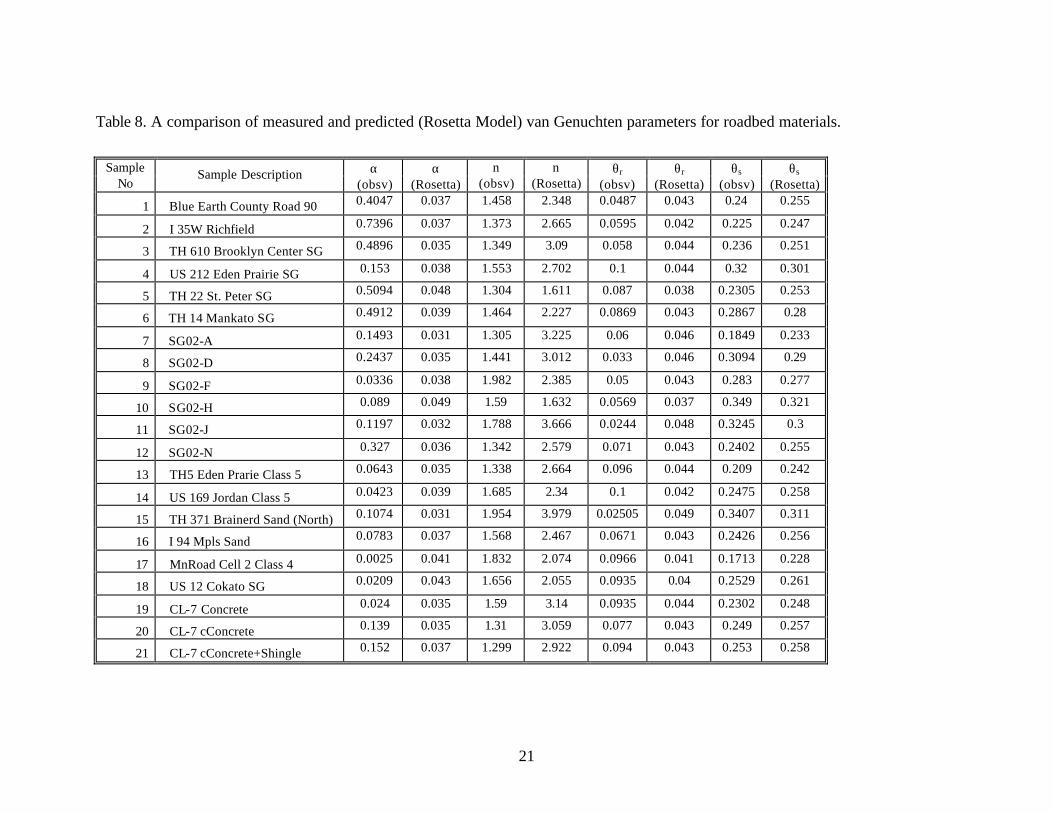
For the Fredlund and Xing’s function model, af ranged from 0.004 to 21.7 kPa for non-recycled material, and 0.53 to 3.34 for recycled materials (Table 7). The values of hr (kPa), varied from 1.43 to 52.8 for non-recycled material and 6.46 to 17.12 for recycled materials. The value of mf ranged from 0.04 to 0.89 for non-recycled material and 0.073 to 0.11 for recycled materials. Comparatively, nf values ranged from 0.58 to 20.0 for non-recycled material and 16.13 to 20.0 for recycled materials. Values of van Genuchten’s parameters obtained in this study were also tested against the prediction from the Rosetta Model (Table 8). Rosetta model predictions are based on the literature values that mainly encompass the agricultural soils. In general, there was very little variation in α values for various samples as predicted from the Rosetta model (Fig. 10). However, the n values predicted from the Rosetta model were higher than those measured in this study (Fig. 11). Although θs values predicted from the Rosetta model were close to the measured values (Fig. 12), θr values predicted from the Rosetta model were higher than the measured values (Figs. 13). This is expected considering that agricultural soils (Rosetta model) are finer, relatively loose, and contain higher organic matter content than the roadbed materials. Also, θr values predicted from the Rosetta model were nearly the same for all samples. Regression analysis was also run to see if there exists relationships between van Genuchten parameters (Eq. [2]) and the particle size analysis. Table 9 lists various best- fit regression equations. These regression equations were developed using the step-wise regression approach (Appendix F). As expected, R2 values increased when second-order terms were included in the regression. For practical application, regression equations with second-order terms appeared to be reasonable for predicting water retention characteristics using van Genuchetn’s function. Regression relationships of van Genuchten’s parameters with gradation indices such as D60 and D10 (Table 10) or gradation number (Table 11) were poor compared to similar relationships with particle size analysis. This is somewhat expected because (1) some gradation indices are based on one or two values on the particle size distribution curve and do not say much about the shape of the curve which really determines the water retention, and (2) other gradation indices include particle sizes that are >2 mm diameter that are shown not to contribute to water retention of soil materials. Regression equations with gradation number (Table 11) were slightly better than those with D60 and D10. Similar to above analysis, step-wise regression analysis was also done for Brooks-Corey parameters (Eq. [5]) and Fredlund-Xing parameters (Eq. [7]) with particle size analysis (Tables 12 and 15) or gradation indices (Tables 13, 14, 16, and 17). Like before, there was poor correlation between Brooks-Corey and Fredlund-Xing parameters with first order particle size analysis and bulk density (Tables 12 and 15). However, when second-degree variables were included, correlation coefficient improved significantly (Appendix G--Brooks-Corey and Appendix H--Fredlund-Xing). The improvement in correlation coefficient with second-degree variables was much higher for Brooks-Corey and Fredlund-Xing parameters than for the van Genuchten’s parameters. Like earlier analysis, relationship of Brooks-Corey and Fredlund-Xing parameters to particle gradation indices (D60, D10, GN) was poor (Tables 13, 14 and 16, 17).

11
Predictions from Existing Models We also tested the predictions of water retention from two commonly used models from the literature against our data. These models are the regression model of Gupta and Larson (1979) and a physico-empirical model of Arya and Paris (1986). Gupta and Larson (1979) model is a regression based model that was developed using 43 mixtures of soil and dredged sediments. The generic regression equation describing this model is: θp=a x sand% + b x silt% +c x clay % + d x OM % + e x bulk density Eq. [9] where θp is the water content at a given suction; sand, silt, and clay are in percent; OM is the organic matter in percent; and a, b, c, d, and e are empirical coefficients. The values of empirical coefficients at a given suction for the Gupta and Larson model are given in Appendix E. Arya and Paris model is based on the concept that soil water retention curve is similar to the particle size distribution curve and then it is a matter of converting particle amount into pore volume (water content) and particle radii into pore radii (suction). These authors used particle packing along with an empirical coefficient to predict water retention from particle size distribution curve.
nieW
Vp
ii
,...,2,1; =
=
ρν Eq. [10]
∑=
=
=ij
j b
vv V
Vj
i1
θ Eq. [11]
where Vvi is the pore volume per unit sample mass associated with the solid particle in the ith particle-size range, Wi is the solid mass per unit sample mass in the ith particle-size range, Vb is the total bulk volume, ρp is the particle density, and e is the void ratio.
21
)1(
64
=
−αi
iien
Rr Eq. [12]
ii gr
hρ
βγ cos2= Eq. [13]
where ri is the mean pore radius, Ri is the mean particle radius, ni is number of spherical particles in the ith particle-size range, γ is water surface tension , g is acceleration due to

12
gravity, β is contact angle (assumed zero), and α is an empirical parameter with a best value of 1.38. Both Gupta and Larson and Arya and Paris models have extensively been used for predicting water retention of loose agricultural soils (dry bulk densities less than 1.8 Mg m-3). Figures 14 and 15 show two comparisons of predicted and measured water retention for two roadbed materials. In general, Gupta and Larson model predicted well the water retention characteristics for roadbed materials with densities up to 1.95 Mg m-3. But the model did not perform as well for higher bulk densities. This is mainly because the water retention database of Gupta and Larson did not cover high bulk densities such as those used in roadbed construction. Since smaller particles have a greater influence on water retention in Arya and Paris model, this model didn’t predict well the water retention of roadbed materials (Figs. 14 and 15), because the roadbed materials tested in this study were mostly the sand fraction. Wetting Curves Figures 16 through 19 show a comparison between the wetting and drying water retention curves for four non-recycled road-bed materials. Except for 2 samples (SG02-A, SG02-F), water content differences between wetting and drying curves were relatively small. This is mainly because all roadbed materials had nearly similar particle size distribution. In SG02-A and SG02-F, the differences in water content between the wetting and the drying curves were as large as 0.12 and 0.20 cm3 cm-3. Water Retention of Recycled Materials Figures 20 through 22 show both the wetting and drying curves of Class 7 concrete, and Class 7 crushed concrete with and without shingles. In general, there was a slight difference in water retention of crushed concrete with and without shingles. This is partially because shingle chips were large and imbedded in the concrete and thus did not alter the properties of the concrete. Even though this data show little impact of the shingle on water retention of concrete, presence of shingle chips can alter the flow paths and in some cases it may provide a preferential pathway along the chip surface. Water retention curves for bottom ash samples in included in Appendix D.

13
Chapter 6: DISCUSSION There is limited variation in the water retention characteristics of base and sub-base materials used for road construction in Minnesota. This is mainly because the particle size distributions of all the samples used in this study fall in a relatively narrow range. The major difference between the materials is the presence of large aggregates (>2 mm diameter), which contribute very little to water retention properties but have a strong influence on saturated hydraulic conductivity and thus on saturated water flow and drainage. These large aggregates, especially gravel, may also act as pathways for preferential movement of water. This data suggest that the use of water retention characteristics (more controlled by smaller particles) along with saturated hydraulic conductivity (more controlled by larger aggregates) to predict unsaturated hydraulic conductivity of roadbed materials (Eqs. [2] and [6]) may not be prudent. Studies should be undertaken to develop databases of road-bed materials of various aggregate sizes used in road-bed construction. These databases should then be used to develop Pedo-transfer functions that can predict hydraulic conductivity of materials from simple parameters such as aggregate size distribution or gradation indices. Several different types of Pedo-transfer function models are given in this report that can be used to predict water retention characteristics of base and sub base materials. These models include simple regression models that predict water retention at a given suction us ing bulk density and particle size distribution. Other models predict function (van Genuchten, Brooks-Corey, and Fredlund-Xing) parameters using similar input variables. However, one should be careful in using predicted function parameters to predict hydraulic conductivity using van Genuchten or Brook and Corey equations [Eqs. [2] and [6]). This is mainly because all three functions depend heavily on measured saturated hydraulic conductivity, which is mainly controlled by large aggregates.

14
Chapter 7: EXPECTED BENEFITS Pavement aggregate base and sub-base are constructed under unsaturated conditions, generally around 90% of optimum water content at maximum density (Standard Proctor). The influence of matric suction has traditionally not been directly considered in pavement design. This is one of the key limitations in the design procedure because matric suction has a significant influence on engineering behavior of pavements related to the soil volume change, coefficient of permeability, freeze-thaw susceptibility, and the shear strength and modulus of pavement aggregate layers. One of the features of Minnesota Flexible Pavement Design Program (MnPAVE), Mn/DOT’s mechanistic-empirical pavement design software, is consideration of the effect of soil moisture on thickness design. Pore suction resistance factors are proposed as a means of incorporating variably saturated material conditions into pavement thickness design. Pore suction resistance factors are proposed for aggregate base by identifying the relationship between suction and resilient modulus. The water retention data in this report will be helpful in developing these resistance factors either through physical modeling or through statistical relationships between design criteria and the water contents.

15
REFERENCES
Arya, L.R. and J.F. Paris. 1986. A physico-empirical model to predict the soil moisture
characteristics from particle size distribution and bulk density data. Soil Sci. Soc. Am. J. 45: 1023-1030.
Brooks, R.H. and A.T. Corey. 1964. Hydraulic properties of porous media. Hydrol. Paper. 3,
Colorado State University, Fort Collins, CO. Campbell, G.S. 1974. A simple method for determining unsaturated conductivity from
moisture retention data. Soil Sci. 117: 311-314. Davich, P., J.F. Labuz, B. Guzina, and A. Drescher. 2004. Small grain and resilient modulus
testing of granular soils. Final Report 2004-39, Minnesota Department of Transportation.
Fredlund, D.G. and A. Xing. 1994. Equations for the soil-water characteristics curve.
Canadian Geotechnical J. 31: 521-532. Gupta, S. C. and Larson W. E. 1979. Estimating soil water retention characteristics from
particle size distribution, organic matter percent, and bulk density. Water Resources. Res. 1633-1635.
Gupta, S.C. and Dong Wang. 2002. Soil Water Retention. In Encyclopedia of Soil Science.
Marcel Dekker, Inc. 1393-1398. Kramer, C. and S. Dai. 2004. Improvement and validation of Mn/DOT DCP specifications for
aggregate base materials and select granular. Interim Report Office of Materials, Minnesota Department of Transportation.
Mualem, Y. 1976. A new model for predicting the hydraulic conductivity of unsaturated
porous media. Water Resour. Res. 12: 593-622. Mm/DOT Office of Materials Grading and Base Manual (2002).
(http://mnroad.dot.state.mn.us/pavement/GradingandBase/gradingandbase.asp) Rawls, W.J., and D.L. Brakensiek. 1982. Estimating soil water retention from soil properties.
J. Irrig. Drain. Eng. 108 (IR2):166-171. Rawls, W. J., D.L. Brakensiek, and K.E. Sexton. 1982. Estimation of soil properties. Trans.
ASAE 25: 1316-1320, 1328.

16
Roberson, R., A. Singh, S. Allaire and S.C. Gupta. 2004. Modeling and measurement strategies for studying contaminant transport below and around highways. Paper presented at the International workshop on “Water Movement and Reactive Transport Modeling in Roads”, Portsmouth, NH, 21-24 February, 2004.
SAS Institute. 2004. The SAS system for Windows. Release 2003. SAS Institute, Cary, NC. SoilVision, User’s Guide. Version 2.0, 1st edition. SoilVision Systems Ltd. Saskatoon,
Saskatchewan, Canada SYSTAT Software. 1996. Version 6.0 for Windows. SPSS Inc. Richmond, CA. van Genuchten, M. Th. 1980. A closed-form equation for predicting the hydraulic
conductivity of unsaturated soils. Soil Sci. Soc. Am. J. 44: 892-898. van Genuchten, M.Th., F.J. Leij, and L. Lund. 1992. Indirect Methods for estimating the
hydraulic properties of unsaturated soils media. Proc. Int. Workshop, University of California, Riverside, CA.
van Genuchten, M.Th., F.J. Leij, and L. Wu. 1999. Characterization and measurements of the
hydraulic properties of unsaturated porous media. Proc. Int. Workshop, University of California, Riverside, CA.

17
Table 1. Gradation number (GN) and optimum moisture content with Proctor Density. Samples 1 to 18 are non-recycled materials; samples 19 to 21 are recycled Class 7 materials); and samples 22 to 25 are recycled bottom ash materials.
Sample No. Sample Sites GN CGN† FGN†
% passing # 200 sieve
OptimumMoisture Content
(%)
Max. Dry Proctor Density
(pcf)
Max. Dry Proctor Density
(Mg m-3) 1 Blue Earth County Road 90 4.65 3.59 1.06 6.9 9.2 111.8 1.790 2 I 35W Richfield 4.19 3.41 0.78 5.0 4.3 128.1 2.052 3 TH 610 Brooklyn Center SG 5.14 3.76 1.38 0.0 4.2 126.4 2.025 4 US 212 Eden Prairie SG 5.52 3.91 1.61 8.0 9.1 111.8 1.790 5 TH 22 St. Peter SG 4.59 3.62 0.97 11.9 5.1 127.3 2.039 6 TH 14 Mankato SG 5.44 3.93 1.51 10.2 7.6 118.0 1.890 7 SG02-A 3.53 2.78 0.75 3.6 7.9 134.7 2.160 8 SG02-D 4.75 3.66 1.09 4.3 10.0 114.8 1.830 9 SG02-F 5.97 3.97 2.00 10.3 9.3 118.6 1.900
10 SG02-H 6.18 4.00 2.18 21.4 12.6 107.7 1.725 11 SG02-J 5.85 4.00 1.85 2.0 9.5 111.8 1.790 12 SG02-N 5.00 3.82 1.18 7.4 8.8 125.7 2.013 13 TH 5 Eden Prairie 3.67 3.11 0.56 3.4 6.4 130.8 2.095 14 US 169 Jordan 4.56 3.56 1.00 7.2 4.8 124.5 1.994 15 TH 371 Brainerd Sand (North) 4.81 3.75 1.06 0.5 7.2 109.1 1.747 16 I 94 Mpls Sand 4.83 3.65 1.18 8.0 3.8 125.3 2.007 17 MnRoad Cell 52 4.41 3.54 0.87 9.2 7.5 137.1 2.196 18 US 12 Cokato 4.32 3.43 0.89 8.0 5.2 123.6 1.980 19 CL 7 Concrete 3.82 3.23 0.60 5.3 8.8 127.4 2.040 20 CL-7 Crushed Concrete 4.52 3.46 1.06 7.3 9.6 124.4 1.990 21 CL-7 cConcrete+Shingles 4.50 3.48 1.02 8.0 10.1 124.0 1.980 22 Bottom Ash C 3.03 2.57 0.46 6.3 19.6 110.0 1.760 23 Bottom Ash D 2.74 2.33 0.41 5.4 14.2 116.8 1.870 24 Bottom Ash E 3.24 2.71 0.53 7.8 15.7 112.5 1.800 25 Bottom Ash F 3.22 2.69 0.53 7.7 19.2 111.8 1.790
† CGN and FGN are coarse and fine gradation numbers, respectively.

18
Table 2. Particle size distribution of road-bed materials assuming 2 mm aggregates were the largest aggregates present. Bulk density values are the Proctor densities (Mg M-3) supplied by Mn/DOT.
Samples Types Sand, Silt, Clay, Bulk Density
Select Granular 78.6 – 99.3 0.48 -16.58 0.17 - 3.00 1.72-2.16 CL-5 88.2 - 89.8 8.19 - 9.60 1.02 - 3.00 1.99-2.09 CL-4 82.48 13.65 3.87 2.19 Non-Recycled 78.6 - 99.3 0.48 -16.58 0.17 - 5.93 1.72-2.19 Recycled (CL-7) 92-93 7.00-8.00 1.98-2.04
Table 3. Regression coefficients (a, b, c) of the Pedo-transfer model for predicting water content (θp) at a given suction. θp = a + b x sand (%) + c x BD (Mg m-3)
Suction (cm) a b c Probability R2
1.0 0.9765 0.00 -0.3686 0.0001 0.985 10.2 0.6004 0.00 -0.2062 0.0129 0.4153 102 0.2711 -0.00433 0.1253 0.0086 0.4626 306 0.1599 -0.00417 0.1633 0.0048 0.6200 510 0.135 -0.00400 0.1623 0.0030 0.6513 714 0.1246 -0.00380 0.1580 0.0027 0.6600
1020 0.1162 -0.00360 0.1525 0.0026 0.6623 3060 0.1013 -0.00325 0.1388 0.0032 0.6488 5100 0.0966 -0.00314 0.1300 0.0035 0.6417
10200 0.0927 -0.00304 0.1314 0.0040 0.6337 15300 0.091 -0.00300 0.1299 0.0043 0.6290

19
Table 4. Sand and silt contents along with dry bulk density for 8 independent samples used to test the Pedo-transfer function model developed in this study.
Sample Sand (% )
Silt (% )
B.D. (Mg m-3)
TH 371 Brainerd, Class 6 93.5 6.5 2.19 Mn Road Class 5 96.5 5.5 1.92 Mn Road Class 6 (crushed granite) 97.5 4.5 1.92 Mn Road Class 4 99.0 1.0 2.02 TH 371 Brainerd, SG 94.0 6.0 1.81 US 169 Mille Lacs 93.0 7.0 2.11 TH 25 Monticello, Class 6 93.5 6.5 2.12 Blue Earth Cty Rd 90, Class 3 91.5 8.5 1.70
Table 5. Range of van Genuchten parameters for different classes of road bed materials.
Samples Types α n θr θs Air Entry
Value Selected Granular
0.020-0.51 1.30-1.98 0.02-0.10 0.18-0.35 1.96-40
Class-5 0.04-0.74 1.34-1.68 0.05-0.10 0.21-0.25 1.35-25 Class-4 0.0025 1.57 0.067 0.17 500
Non-Recycled 0.0025-0.74 1.30-1.98 0.02-0.10 0.17-0.34 1.35-500 Recycled 0.024-0.15 1.3-1.59 0.08-0.09 0.23 - 0.25 6.57-41.7

20
Table 6. Range of Brooks and Corey parameters for different classes of road bed materials.
Samples Types aC nC
Selected Granular 0.15-2.16 0.255-0.775 Class-5 0.132-0.856 0.084-0.385 Class-4 9.894 0.127
Non-Recycled 0.132-9.894 0.084-0.775 Recycled 0.429-2.295 0.244-0.395
Table 7. Range of Fredlund and Xing parameters for different classes of road bed materials.
Samples Types af hR mF nF
Selected Granular 0.004-3.06 3.26-27.96 0.14-0.881 0.58-7.27 Class-5 0.008-1.564 1.43-7.90 0.039-0.629 1.01-20.0 Class-4 21.65 52.81 0.040 20.0
Non-Recycled 0.004-21.65 1.43-52.81 0.039-0.885 0.579-20.0 Recycled 0.53-3.34 6.46-17.12 0.073-0.106 16.13-20.0
21
Table 8. A comparison of measured and predicted (Rosetta Model) van Genuchten parameters for roadbed materials.
Sample
No Sample Description α
(obsv) α
(Rosetta) n
(obsv) n
(Rosetta) θr
(obsv) θr
(Rosetta) θs
(obsv) θs
(Rosetta)
1 Blue Earth County Road 90 0.4047 0.037 1.458 2.348 0.0487 0.043 0.24 0.255
2 I 35W Richfield 0.7396 0.037 1.373 2.665 0.0595 0.042 0.225 0.247
3 TH 610 Brooklyn Center SG 0.4896 0.035 1.349 3.09 0.058 0.044 0.236 0.251
4 US 212 Eden Prairie SG 0.153 0.038 1.553 2.702 0.1 0.044 0.32 0.301
5 TH 22 St. Peter SG 0.5094 0.048 1.304 1.611 0.087 0.038 0.2305 0.253
6 TH 14 Mankato SG 0.4912 0.039 1.464 2.227 0.0869 0.043 0.2867 0.28
7 SG02-A 0.1493 0.031 1.305 3.225 0.06 0.046 0.1849 0.233
8 SG02-D 0.2437 0.035 1.441 3.012 0.033 0.046 0.3094 0.29
9 SG02-F 0.0336 0.038 1.982 2.385 0.05 0.043 0.283 0.277
10 SG02-H 0.089 0.049 1.59 1.632 0.0569 0.037 0.349 0.321
11 SG02-J 0.1197 0.032 1.788 3.666 0.0244 0.048 0.3245 0.3
12 SG02-N 0.327 0.036 1.342 2.579 0.071 0.043 0.2402 0.255
13 TH5 Eden Prarie Class 5 0.0643 0.035 1.338 2.664 0.096 0.044 0.209 0.242
14 US 169 Jordan Class 5 0.0423 0.039 1.685 2.34 0.1 0.042 0.2475 0.258
15 TH 371 Brainerd Sand (North) 0.1074 0.031 1.954 3.979 0.02505 0.049 0.3407 0.311
16 I 94 Mpls Sand 0.0783 0.037 1.568 2.467 0.0671 0.043 0.2426 0.256
17 MnRoad Cell 2 Class 4 0.0025 0.041 1.832 2.074 0.0966 0.041 0.1713 0.228
18 US 12 Cokato SG 0.0209 0.043 1.656 2.055 0.0935 0.04 0.2529 0.261
19 CL-7 Concrete 0.024 0.035 1.59 3.14 0.0935 0.044 0.2302 0.248
20 CL-7 cConcrete 0.139 0.035 1.31 3.059 0.077 0.043 0.249 0.257
21 CL-7 cConcrete+Shingle 0.152 0.037 1.299 2.922 0.094 0.043 0.253 0.258

22
Table 9. Regression relationships between van Genuchten Parameters and the soil particle analysis and bulk density.
REGRESSION EQUATIONS r2
α = 1.386 + 4.914*Silt - 5.229*Clay - 0.718*BD 0.282 α = 671.129 - 1325.005* Silt - 1276.152* Clay - 17.758*BD + 1.115*BD2 – 669.248* Sand 2 + 2479.904* Clay 2 + 941.681* Silt 2 + 14.792*BD*Sand
0.778
n = 2.764 - 0.855* Silt + 1.390* Clay - 0.598*BD 0.221 n = -102.401 + 180.496* Sand + 35.003* Clay + 11.987*BD - 72.496* Sand 2 -267.303* Clay 2 + 156.226* Silt 2 - 14.103*BD* Sand 0.630
θs = 0.999 - 0.018* Silt + 0.043* Clay - 0.376*BD 0.999 θr = -160 + 0.094* Sand + 0.438* Silt + 0.055*BD 0.441 θr = 0.009 + 0.272*BD - 17.315* Clay 2 - 0.264*BD* Sand 0.512
Table 10. Regression between van Genuchten Parameters and gradation indices (D60 and D10).
REGRESSION EQUATIONS r2
α = 0.398 - 0.006*D60 - 0.849*D10 0.067 α = 1.064-0.250*D60-10.033*D10-0.044*D602+17.898*D102+3.451*D60*D10 0.513
n = 1.555 - 0.034*D60 + 0.586*D10 0.201 n = 1.719 - 2.153*D10 + 0.005*D602+ 9.373*D102 - 0.407*D60*D10 0.289 θs = 0.264 - 0.012*D60 + 0.174*D10 0.424 θs = 0.383 -0.053*D60-1.206*D10-0.001*D602+ 3.311*D102+0.260*D60*D10
0.778
θr = 0.088 + 0.004*D60 - 0.227*D10 0.397 θr = 0.065+0.016*D60+0.039*D10+0.001*D602-0.441*D102-0.123*D60*D10
0.453

23
Table 11. Regression relationships between van Genuchten Parameters and gradation numbers (CGN and FGN). CGN and FGN are coarse (4.75 to 25 mm diameter aggregates) and fine (0.075 to 2.0 mm diameter aggregates) gradation numbers (Eq. 1).
Table 12. Regression between Brooks and Corey Parameters and soil particle analysis and bulk density.
REGRESSION EQUATION R2 α = -0.021 + 0.035*CGN + 0.135 *FGN 0.071 α = 4.497 - 4.867*CGN + 7.277*FGN + 1.179*CGN2 + 1.408*FGN2 - 2.962*CGN x FGN 0.181
n = 0.688 + 0.215*CGN + 0.069*FGN 0.190 n= 1.544 -1.134*CGN + 2.695*FGN + 0.390*CGN2 + 0.669*FGN2 - 1.202*CGN x FGN 0.238
θs = -0.039 + 0.068*CGN + 0.043*FGN 0.566 θs = 1.271 - 0.786*CGN + 0.142*FGN + 0.148*CGN2 + 0.065*FGN2 - 0.091*CGN x FGN 0.590
θr = 0.077 + 0.004*CGN - 0.021*FGN 0.104 θr = -1.094 + 0.944*CGN - 0.811*FGN - 0.182*CGN2 - 0.095*FGN2 + 0.286*CGN x FGN 0.195
REGRESSION EQUATIONS r2 ac = 0.436 - 10.830*Sand + -3.559*Clay + 5.335*BD 0.208 ac = - 10.394 + 7.319*Clay + 10.800*Silt + 5.337*BD 0.208 ac = - 2.800 + 3.106*Silt - 7.601*Sand+ 5.341*BD 0.208
ac = 13425.675 -16961.379*Sand - 10896.403*Silt - 5671.317*Clay + 610.254*BD + 3785.301*Sand2 - 55507.301*Silt2 - 13779.648*Clay2+ 54.551*BD2 -848.026*BD*Sand - 2813.088*BD*Clay
0.922
nC = 1.592 + 0.837*Sand - 0.625*Clay - 0.982*BD 0.670 nC = 2.429 - 1.461*Clay – 0.837*Silt – 0.982*BD 0.669 nC = 0.957 + 1.472*Sand + 0.639*Silt – 0.982*BD 0.670

24
Table 13. Regression between Brooks and Corey Parameters and gradation indices (D60 and D10).
REGRESSION EQUATIONS r2
ac = 1.805 + 0.103*D60 - 6.790*D10 0.039 ac = -0.873 + 2.115*D60 + 14.390*D10 + 0.106*D602 - 17.354*D102 - 15.069*D60*D10
0.235
nC = 0.364 -0.036*D60 + 0.915*D10 0.301 nC = 0.708 - 0.142*D60 - 3.240*DT - 0.003*D602 + 10.331*D102 + 0.669*D60*D10
0.505
Table 14. Regression between Brooks & Corey Parameters and gradation numbers (CGN and FGN). CGN and FGN are coarse (4.75 to 25 mm diameter aggregates) and fine (0.075 to 2.0 mm diameter aggregates) gradation numbers (Eq. 1).
Equations R2
ac = -0.999 + 1.033*CGN - 1.339*FGN 0.029 ac = -8.520 -4.310*CGN + 30.702*FGN + 3.008*CGN2 + 8.199*FGN2 - 14.509*CGN x FGN 0.115
nc = -0.284 + 0.129 *CGN + 0.179 *FGN 0.364 nc = 6.431 - 3.812*CGN - 0.756*FGN + 0.603*CGN2 + 0.012*FGN2 + 0.154*CGN x FGN 0.422
Table 15. Regression relationships between Fredlund and Xing Parameters and the soil particle analysis and bulk density.
REGRESSION EQUATIONS r2
af = - 6.955 - 18.046*Sand + 4.371*Silt + 12.549*BD 0.218 af = -352.900 + 5880.153*Clay + 466.563*BD + 1023.602*Sand2 -1577.359*Silt2 - 8635.957*Clay2 + 154.391*BD2 - 1118.018*BD*Sand - 2972.789*BD*Clay
0.915
hr = - 439.426 + 391.528*Sand + 586.174*Silt + 26.338*BD 0.291 hr = -16957.844 + 29913.633*Silt + 54074.753*Clay + 2680.515*BD + 18333.244*Sand2 - 27891.967* Silt2 - 55489.594*Clay2 + 311.442*BD2 - 4007.585*BD*Sand - 13780.133*BD*Clay
0.668
mf = 2.729 - 2.533*Silt -0.853*Clay - 1.085*BD 0.617 nf = - 87.487 + 50.125*Sand + 90.296*Silt + 20.677*BD 0.241 nf = 46688.085 - 78043.667*Sand - 19827.491*Silt + 2861.115*BD + 31665.996*Sand2 -45537.825*Silt2 - 102480.886*Clay2 + 54.414*BD2 - 3133.604*BD*Sand - 11762.812*BD*Clay
0.612

25
Table 16. Regression relationships between Fredlund and Xing Parameters and gradation indices (D60 and D10).
REGRESSION EQUATIONS r2
af = 3.135 - 13.185*D10 + 0.219*D60 0.031 af = -2.885 + 34.214*D10+ 4.669* D60 – 42.835*D102 + 0.212*D602 - 32.202*D10*D60 0.232
hr = 13.728 - 24.081*D10 + 0.202*D60 0.015 hr = - 8.797 + 215.863*D10 + 11.774*D60 - 428.641*D102 + 0.790*D602 - 96.776*D10*D60
0.259
mf = 0.198 + 2.411*D10 - 0.065*D60 0.558 mf = 0.318 + 1.351*D10 -0.113*D60 + 2.966*D102 + 0.005*D602 0.597 nf = 4.454 - 14.174*D10 + 1.200*D60 0.259 nf = -1.636 + 66.995*D10 + 4.018*D60 -132.595*D102+ 0.503*D602 - 39.665*D10*D60
0.338
Table 17. Regression between Fredlund & Xing Parameters and gradation numbers (CGN and FGN). CGN and FGN are coarse (4.75 to 25 mm diameter aggregates) and fine (0.075 to 2.0 mm diameter aggregates) gradation numbers (Eq. 1).
Equation R2 af = -4.189 + 2.871*CGN - 3.604*FGN 0.042 af = 7.870 - 30.0*CGN + 79.167*FGN + 10.511*CGN2 + 19.729*FGN2 - 36.646*CGN x FGN
0.125
hr = 7.633 + 2.349*CGN - 4.291*FGN 0.013 hr = -300.842 + 135.324*CGN + 210.770*FGN - 11.963*CGN2 + 24.338*FGN2 - 70.121*CGN x FGN 0.098
mf = -0.871 + 0.305*CGN + 0.109*FGN 0.266 mf = 5.912 - 4.935*CGN + 4.055*FGN + 0.974*CGN2 + 0.361*FGN2 - 1.348*CGN x FGN 0.296
nf = 21.653 - 2.766*CGN - 5.126*FGN 0.199 nf = -243.818 + 209.641*CGN - 203.247*FGN - 38.388*CGN2 - 4.062*FGN2 + 55.604 *CGN x FGN
0.414

26
Grain Size Distribution Non-Recycled
0%
10%
20%
30%
40%
50%
60%
70%
80%
90%
100%
0.001 0.01 0.1 1 10 100
Grain Size (millimeters)
BlueEarth90
I 35W Richfield
TH 610 Brooklyn Center Select Granular
US 212 Eden Prairie Select Granular
TH 22 St. Peter Select Granular
TH 14 Mankato Select Granular
SG02-A
SG02-D
SG02-F
SG02-H
SG02-J
SG02-N
Th 5 Eden Prarie Class 5
US 169 Jordan Class 5
TH 371 Brainerd Sand (North)
I 94 Mpls Sand
MnRoad Cell 52 Class 4
US 12 Cokato
Figure 1. Particle size distribution for non-recycled road-bed materials.

27
Figure 2. Particle size distribution for non-recycled road-bed materials at maximum grain size of 2.0 mm.
Grain Size Distribution (max. 2mm)
0%
10%
20%
30%
40%
50%
60%
70%
80%
90%
100%
0.001 0.01 0.1 1 10 Grain Size (millimeters)
BlueEarth90 I 35W Richfield TH 610 Brooklyn Center Selecter Granular US 212 Eden Prairie Select Granular TH 22 St. Peter Selected Granular TH 14 Mankato Selected Granular SG02-A SG02-D SG02-F SG02-H SG02-J SG02-N TH5 Eden Prarie Cl5 US169 Jordan Cl5 TH371 Brainerd Sand I94 Mpls Sand MnRoad Cell 52 Cl4 US12 Cokata SG

28
Data Overlap for Water Retention Equipment: Tempe Cells, 3-bar & 15-bar Pressure PlateTH 610 Brooklyn Center SG w/ best fit curve
y = 0.1789x -0.1072
R2 = 0.9565
0.00
0.04
0.08
0.12
0.16
0.20
1 10 100 1000 10000 100000
Matric Potential, -h (cm)
Wat
er C
onte
nt (
cc/c
c)
Tempe Cells3-bar Pressure Plate15-bar Pressure PlateBest-Fit Curve
Figure 3. Measured and fitted water retention curve of select granular from TH610 Brooklyn Center.

29
Characteristic Curves For Non-Recycled
0
0.05
0.1
0.15
0.2
0.25
0.3
0.35
0.4
1 10 100 1000 10000 100000
Matric Potential, -h (cm of Water)
Wat
er C
on
ten
t (v/
v)Blue Eart 90
I35W Richfield
TH 610 Brooklyn
US 212 Eden Prairie
TH 22 St. Peter
TH 14 Mankato
SG02-A
SG02-D
SG02-F
SG02-H
SG02-J
SG02-N
Th 5 Eden Prarie Class 5
US 169 Jordan Class 5
TH 371 Brainerd Sand (North)
I 94 Mpls Sand
MnRoad Cell 52 Class 4
US 12 Cokato
Figure 4. Water retention characteristic (drying) curves for non-recycled road-bed materials.

30
Characteristic Curves For CL-7 (Recycled Material)
0
0.05
0.1
0.15
0.2
0.25
0.3
1 10 100 1000 10000 100000
Matric Potential, -h (cm of Water)
Wat
er C
onte
nt (
v/v)
CL 7 Concrete
CL-7 Crushed Concrete
CL-7 cConcrete+Shingles
Figure 5. Water retention characteristic (drying) curves for Class 7 recycled material.

31
0.00
0.05
0.10
0.15
0.20
0.25
0.30
1 10 100 1000 10000 100000
Head (cm)
θ (v
/v)
MN Road Class 5
Model
Figure 6. Simulation of water retention characteristics (drying) curve for MN Road, Class 5

32
0.00
0.05
0.10
0.15
0.20
0.25
0.30
1 10 100 1000 10000 100000
Head (cm)
θ (v
/v)
MN Road CL6 CG
Model
Figure 7. Simulation of water retention characteristics (drying) curve for MN Road, crushed granite, Class 6.

33
0.00
0.05
0.10
0.15
0.20
0.25
0.30
1 10 100 1000 10000 100000Head (cm)
θ (v
/v)
MN Road CL4
Model
Figure 8. Simulation of water retention characteristics (drying) curve for MN Road,
Class 4

34
0.00
0.10
0.20
0.30
0.40
1 10 100 1000 10000 100000Head (cm)
θ (v
/v)
TH 371 SGModel
Figure 9. Simulation of water retention characteristics (drying) curve for TH 371 Brainerd, Sand (SP-SM), select granular.

35
0.00
0.02
0.04
0.06
0.08
0.10
0.0 0.1 0.2 0.3 0.4 0.5 0.6 0.7 0.8Observed
Mo
del
Rosetta Model for alfa
1-to-1 Line
Figure 10. A comparison of van Genuchten’s α parameter predicted from the Rosetta model vs. the observed values.

36
0.0
1.0
2.0
3.0
4.0
5.0
0.0 0.5 1.0 1.5 2.0 2.5 3.0
Observed
Mo
del
Rosetta Model for n
1-to-1 Line
Figure 11. A comparison of van Genuchten’s n parameter predicted from the Rosetta model vs. the observed values.

37
0.00
0.10
0.20
0.30
0.40
0.50
0.10 0.15 0.20 0.25 0.30 0.35 0.40Observed
Mo
del
Rosetta Model for theta S
1-to-1 Line
Figure 12. A comparison of van Genuchten’s θs parameter predicted from the Rosetta model vs. the observed values.

38
0.00
0.02
0.04
0.06
0.08
0.10
0.00 0.02 0.04 0.06 0.08 0.10 0.12Observed
Mo
del
Rosetta Model for theta R
1-to-1 Line
Figure 13. A comparison of van Genuchten’s θr parameter predicted from the Rosetta model vs. the observed values.

39
Characteristic Curves For US 212 Eden Prairie
00.05
0.10.15
0.20.25
0.30.35
0.01 1 100 10000 1000000
Matric Potential, -h (cm of Water)
Wat
er C
on
ten
t (v/
v)
Observed(BD=1.95)
Arya&Paris
Gupta&Larson
Figure 14. A comparison of predicted water retention characteristic (drying) curves based on Arya & Paris and Gupta & Larson models vs. the measured curve for US 212 Eden Prairie sample.

40
Characteristic Curves For TH 22 St. Peter SG
0
0.05
0.1
0.15
0.2
0.25
0.01 0.1 1 10 100 1000 10000 1E+05
Matric Potential, -h (cm of Water)
Wat
er C
on
ten
t (v/
v)
Observed(BD=2.13)
Arya&Paris
Gupta&Larson
Figure 15. A comparison of predicted water retention characteristic (drying) curves based on Arya & Paris and Gupta & Larson models vs. the measured curve for TH 22 St. Peter SG sample.

41
0.00
0.04
0.08
0.12
0.16
0.20
1 10 100 1000 10000 100000
Matric Potential, -h (cm of Water)
Wat
er C
onte
nt (
v/v) Drying
Wetting
Figure 16. Hysteresis Curves for SG02-A.

42
0.00
0.05
0.10
0.15
0.20
0.25
0.30
0.35
1 10 100 1000 10000 100000
Matric Potential, -h (cm of Water)
Wat
er C
onte
nt (
v/v)
Drying
Wetting
Figure 17. Hysteresis Curves for SG02-D.

43
0.00
0.05
0.10
0.15
0.20
0.25
0.30
1 10 100 1000 10000 100000
Matric Potential, -h (cm of Water)
Wat
er C
onte
nt (
v/v)
Drying
Wetting
Figure 18. Hysteresis Curves for SG02-F.

44
0.00
0.05
0.10
0.15
0.20
0.25
0.30
1 10 100 1000 10000 100000
Matric Potential, -h (cm of Water)
Wat
er C
onte
nt (
v/v) Drying
Wetting
Figure 19. Hysteresis Curves for SG02-N.

45
0.00
0.05
0.10
0.15
0.20
0.25
1 10 100 1000 10000 100000
Matric Potential, -h (cm of Water)
Wat
er C
onte
nt (
v/v)
Drying
Wetting
Figure 20. Hysteresis Curves for Concrete, Class 7.

46
0.00
0.05
0.10
0.15
0.20
0.25
0.30
1 10 100 1000 10000 100000
Matric Potential, -h (cm of Water)
Wat
er C
onte
nt (
v/v) Drying
Wetting
Figure 21. Hysteresis Curves for crushed Concrete, Class 7.

47
0.00
0.05
0.10
0.15
0.20
0.25
0.30
1 10 100 1000 10000 100000
Head (cm)
Wat
er C
onte
nt (
v/v)
Drying
Wetting
Figure 22. Hysteresis Curves for crushed Concrete and shingles, Class 7.

Appendix A Sampling Procedure for Pressure Plate Apparatus, Tempe Cells,
and Wetting Curve

A-1
A1. Sampling Procedure for Pressure Plate Apparatus
Apparatus The apparatus setup for the analysis of road bed soils from a pressure range of 102 – 15300 cm H2O was established in two parts. Two sets of pressure plate apparatus, 5 bar pressure chamber (102 – 3060 cm H2O) and 15 bar pressure chamber (1020 – 15300 cm H2O), comprise the setup for pressure application. Procedure
1. Sample Preparation i) Remove aggregates larger than 3/8th of an inch. This was done because our
cores were only 4 inch in diameter and we wanted to make sure that large aggregates and gravel did not unduly influenced the water desorption.
ii) Since even the small aggregates are not evenly distributed when taking a soil sample for packing, it is better to prepare a large soil sample and have it ready packing of 4-5 rings at one time. This helps achieve uniformity among the packed samples.
iii) Weigh the dry soil required for 5 samples (Data base file “Pressure Plates.mdb”) and put in the polythene bags of size 1.5’x2.5’ and 4 ply thick.
iv) Weigh the water required to attain optimum density in a spray bottle. v) Spray the soil in the bag with waters and shake the bag side by side for
thorough mixing. Seal the bag and keep it for 24 hours. Keep shaking the bag for uniform mixing.
vi) Weigh the sample required for one ring (According to the Data base file “Pressure Plates.mdb”).
2. Packing The Rings i) Take a ring and weigh it. ii) Tape an additional ring at the top of the ring to be filled with soil sample. iii) Place the rings in the can. iv) Weigh the wet soil required for one ring. v) Fill the rings with the soil and place the can with rings in the hydraulic
press. vi) Compress the sample soil in the press until the head of the piston reaches
the top of the upper ring. vii) Remove the can with rings from the hydraulic press. viii) Remove the top ring. ix) Soil in the bottom ring is now compressed to the desired density.

A-2
3. Saturating the Sample i) Spread a small amount of fine clay soil on the pressure plate where the soil
ring will be placed. This helps to improve the contact surface between plate and the soil in the ring.
ii) Gently, embed the sample ring into the clay layer on the ceramic plate. iii) Take a dish washing bucket and fill it half with water (preferably
deionized). iv) Place three 1” rings in the dish. v) Place the ceramic plate with sample ring on the top of the rings. vi) Add the water in the bucket so that almost 3/4th of the ring is submerged in
water. vii) Allow the sample and the ceramic plate to saturate for 2-3 days and the top
of the soil glistens.
4. Using the Pressure Plates i) Place the saturated ceramic plate with sample on the top in a pressure
chamber (5-bar or 15-bar, as planned). ii) Attach the outlet on the ceramic plate to the outlet on the pressure
chamber with a small diameter neoprene tube. iii) Place the lid at the top of the pressure chamber and tighten the two screws
(cross-wise) at a time until the chamber if fully tightened. iv) Insert the drain tube from the pressure chamber to a burette used for
recording the quantity of water coming out of the sample. v) Attach the pressure hose of the pressure chamber to a pressurized air outlet
connected to a compressor. vi) Apply the desired pressure.
5. Measuring the Water Loss
i) Record the water in the burette at different time intervals till the water stops draining out of the sample.
ii) Shift to the next pressure (if required) and repeat the first step. iii) Release the pressure in the chamber when a given set of pressure range is
completed. iv) Remove the ceramic plate from the chamber. v) Take out of the sample ring and weigh out the sample.
vi)
6. Drying the Sample
i) Since the samples contain some aggregates and stones, entire sample is emptied into a can for drying.
ii) Set the temperature of the oven at 1050 C and dry the soil for 24 hrs. iii) Weigh the dried sample.

A-3
7. Developing Moisture Curves
i) Enter the data into pressure plate calculation spreadsheet. ii) The spread sheet calculates the moisture content at each pressure. iii) Plot the moisture retention curves.
A2. Sampling Procedure for Tempe Cell Apparatus Apparatus The Tempe cell apparatus is used for moisture retention at small pressure ranges (10.2 – 1020 cm H2O) Two different ceramic plates with bubbling pressures of 0.5 and 1.0 bars were used in Tempe Cells desorption measurements. Procedure
1. Sampling Calculation: Use procedure described in program module “pressure Plates.mdb” (Fig. 1) to calculate amount of dry soil, water needed to achieve optimum moisture content and weight of wet soil required per ring.
2. Sample Preparation a. Remove aggregates larger than 3/8th of an inch. This was done because our
cores were only 4 inch in diameter and we wanted to make sure that large aggregates and large stones did not unduly influenced the water desorption.
b. Since even the small aggregates are not evenly distributed when taking a soil sample for packing, it is better to prepare a large soil sample and have it ready packing of 4-5 rings at one time. This helps achieve uniformity among the packed samples.
c. Weigh the dry soil required for 5 samples (Data base file “Pressure Plates.mdb”) and put in the polythene bags of size 1.5’x2.5’ and 4 ply thick.
d. Weigh the water required to attain optimum density in a spray bottle. e. Spray the soil in the bag with waters and shake the bag side by side for
thorough mixing. Seal the bag and keep it for 24 hours. Keep shaking the bag for uniform mixing.
f. Weigh the sample required for one ring (According to the Data base file “Pressure Plates.mdb”).
3. Packing The Rings a. Take a ring and weigh it. b. Tape an additional ring at the top of the ring to be filled with soil sample. c. Place the rings in the can. d. Weigh the wet soil required for one ring. e. Fill the rings with the soil and place the can with rings in the hydraulic press. f. Compress the sample soil in the press until the head of the piston reaches the
top of the upper ring. g. Remove the can with rings from the hydraulic press.

A-4
h. Remove the top ring. i. Soil in the bottom ring is now compressed to the desired density.
4. Saturating the Sample a. Place the sample ring on the ceramic plate rated for the planned test pressure
fixed to the bottom part of the Tempe Cell. b. Press the sample ring tight in the O-ring of the Tempe cell. c. Take a dish washing bucket and fill it half with water (preferably deionized). d. Place a 1” rings in the bucket. e. Place the Tempe Cell with sample ring in it. f. Add the water in the bucket so that almost 3/4th of the ring is submerged in
water. g. Allow the sample and the plate to saturate for 2-3 days or till the top of the
soil glistens. 5. Using the Tempe Cells
a. Cover the top of the sample ring with the top part of the Tempe Cell and tighten two screws (cross-wise) at a time until it is fully tightened.
b. Put the drain tube of the Tempe Cell into a burette for recording the quantity of water that is draining from the sample.
c. Attach the pressure hose of the pressure chamber to the compressed air set-up and apply the desired pressure.
6. Measuring the Water Loss
a. Record the water in the burette at different time intervals till the water stops draining out of the sample.
b. Shift to the next pressure (if required) and repeat the first step. c. When the sample has gone through all required pressure steps, release the
pressure. d. Remove the sample from the Tempe Cell. e. Weigh the sample.
7. Drying the Sample a. Since the samples contain some aggregates and stones, entire sample is
emptied into a can for drying. b. Set the temperature of the oven at 1050 C and dry the soil for 24 hrs. c. Weigh the dried sample.
8. Developing Moisture Curves a. Enter the data into pressure plate calculation spreadsheet. b. The spreadsheet calculates the moisture content at each pressure. c. Plot the moisture retention curves.
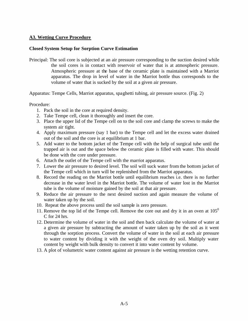
A-5
A3. Wetting Curve Procedure
Closed System Setup for Sorption Curve Estimation Principal: The soil core is subjected at an air pressure corresponding to the suction desired while
the soil cores is in contact with reservoir of water that is at atmospheric pressure. Atmospheric pressure at the base of the ceramic plate is maintained with a Marriot apparatus. The drop in level of water in the Marriot bottle thus corresponds to the volume of water that is sucked by the soil at a given air pressure.
Apparatus: Tempe Cells, Marriot apparatus, spaghetti tubing, air pressure source. (Fig. 2) Procedure:
1. Pack the soil in the core at required density. 2. Take Tempe cell, clean it thoroughly and insert the core. 3. Place the upper lid of the Tempe cell on to the soil core and clamp the screws to make the
system air tight. 4. Apply maximum pressure (say 1 bar) to the Tempe cell and let the excess water drained
out of the soil and the core is at equilibrium at 1 bar. 5. Add water to the bottom jacket of the Tempe cell with the help of surgical tube until the
trapped air is out and the space below the ceramic plate is filled with water. This should be done with the core under pressure.
6. Attach the outlet of the Tempe cell with the marriot apparatus. 7. Lower the air pressure to desired level. The soil will suck water from the bottom jacket of
the Tempe cell which in turn will be replenished from the Marriot apparatus. 8. Record the reading on the Marriot bottle until equilibrium reaches i.e. there is no further
decrease in the water level in the Marriot bottle. The volume of water lost in the Marriot tube is the volume of moisture gained by the soil at that air pressure.
9. Reduce the air pressure to the next desired suction and again measure the volume of water taken up by the soil.
10. Repeat the above process until the soil sample is zero pressure. 11. Remove the top lid of the Tempe cell. Remove the core out and dry it in an oven at 1050
C for 24 hrs. 12. Determine the volume of water in the soil and then back calculate the volume of water at
a given air pressure by subtracting the amount of water taken up by the soil as it went through the sorption process. Convert the volume of water in the soil at each air pressure to water content by dividing it with the weight of the oven dry soil. Multiply water content by weight with bulk density to convert it into water content by volume.
13. A plot of volumetric water content against air pressure is the wetting retention curve.

A-6
Precautions: 1. Desired core dimensions (6cm x 3 cm). 2. Clean Tempe cell thoroughly so that there is no soil grains struck to o-rings. 3. Oil the o-rings of the Tempe cell so that the soil easily for core to easily slides and sit
properly on the ceramic plate. 4. Check for any pressure leakage. 5. Bleed all the trapped air from the system for proper flow of water from the Marriot bottle
system to the Tempe cell. Advantages:
1. The system replicates the dry front procedure. 2. Since the system is closed, there are no evaporation losses.
A wide range of pressure could be applied which is not possible with the hanging water columns.

Appendix B
Particle Size Distribution for non-recycled and recycled samples

B-1
Table B1. Particle size distribution for non-recycled samples
Blue Earth County Road 90
I 35W Richfield
TH 610 Brooklyn
Center SG
US 212 Eden Prairie
SG
TH 22 St. Peter SG
TH 14 Mankato SG
English Metric (mm)
2 1/2 63.0
2" 50.0
1 1/2" 37.5
1 1/4" 31.5
1" 25.0 100 100 100 100 100 100
3/4" 19.0 96.0 95.0 96.4 99.2 96.9 100.0
5/8" 16.0
1/2" 12.5 86.5 94.5 98.6 92.2 98.8
3/8" 9.5 85.7 80.5 91.6 97.8 89.6 97.7
#4 4.75 77.4 65.2 88.3 94.3 75.9 95.0
#8 2.36 51.9 82.4 89.9 61.0 90.1
#10 2.00 64.9 50.0 82.0 88.0 58.0 89.0
#16 1.18 40.3 73.6 83.9 47.4 86.4
#30 0.600 28.6 52.9 76.4 33.9 80.7
#40 0.425 34.4 23.0 55.8 65.0 27.0 52.0
#50 0.300 15.1 14.2 53.6 20.1 26.1
#100 0.150 10.5 7.5 2.0 18.5 14.4 13.6
#200 0.075 6.9 5.0 8.0 11.9 10.2
Sieve Size

B-2
Table B2. Particle size distribution for non-recycled samples
SG02-A SG02-D SG02-F SG02-H SG02-J SG02-N
English Metric (mm)
2 1/2 63.0 100.0 100.0 100.0 100.0 100.0 100.02" 50.0 94.0 100.0 100.0 100.0 100.0 100.0
1 1/2" 37.5 90.0 100.0 100.0 100.0 100.0 100.01 1/4" 31.5 87.0 98.0 100.0 100.0 100.0 100.0
1" 25.0 81.0 97.0 100.0 100.0 100.0 100.0
3/4" 19.0 77.0 95.0 100.0 100.0 100.0 100.0
5/8" 16.0 73.0 94.0 100.0 100.0 100.0 100.0
1/2" 12.5 69.0 93.0 100.0 100.0 100.0 98.0
3/8" 9.5 65.0 90.0 99.0 100.0 100.0 96.0
#4 4.75 55.0 84.0 98.0 100.0 100.0 86.0
#8 2.36 48.0 76.0 98.0 100.0 100.0 76.0
#10 2.00 47.0 74.0 98.0 100.0 100.0 73.0
#16 1.18 41.0 65.0 98.0 99.0 100.0 64.0
#30 0.600 30.0 44.0 96.0 98.0 93.0 48.0
#40 0.425 24.0 31.0 92.0 97.0 83.0 38.0
#50 0.300 16.0 18.0 78.0 91.0 64.0 28.0
#100 0.150 7.0 6.0 29.0 53.0 21.0 12.0
#200 0.075 3.6 4.3 10.3 21.4 2.0 7.4
Sieve Size

B-3
Table B3. Particle size distribution for non-recycled and recycled samples (concrete)
TH 5 Eden Prairie
US 169 Jordan
TH 371 Brainerd
Sand (North)
I 94 Mpls Sand
MnRoad Cell 52
US 12 Cokato
CL 7 Concrete
CL-7 Crushed Concrete
CL-7 cConcrete+
Shingles
English Metric (mm)
2 1/2 63.0 100.0 100.0 100.0 100.0 100.0 100.0 100.0 100.0 100.02" 50.0 100.0 100.0 100.0 100.0 100.0 100.0 100.0 100.0 100.0
1 1/2" 37.5 100.0 100.0 100.0 100.0 100.0 100.0 100.0 100.0 100.01 1/4" 31.5 100.0 100.0 100.0 100.0 100.0 100.0 100.0 100.0 100.0
1" 25.0 100.0 100.0 100.0 98.9 100.0 100.0 100.0 100.0 100.03/4" 19.0 97.3 93.5 97.3 94.5 97.9 94.7 98.3 96.4 97.9
5/8" 16.0 86.9 90.6 96.4 92.8 95.0 90.6 95.7 92.4 94.0
1/2" 12.5 74.3 88.1 94.3 90.5 91.2 84.0 86.0 87.0 89.63/8" 9.5 64.4 85.0 92.3 88.2 84.5 79.8 72.5 80.8 82.6
#4 4.75 49.3 77.6 85.8 83.1 71.3 68.1 51.7 69.1 67.6#8 2.36 37.4 69.7 79.3 77.4 57.9 56.7 39.2 62.3 61.2
#10 2.00 33.1 60.0 76.6 72.9 51.5 53.3 36.7 60.6 59.4#16 1.18 27.5 53.7 69.9 70.0 44.9 41.2 30.4 55.2 53.3
#30 0.600 22.8 45.7 56.0 57.4 32.1 30.2 21.7 45.1 41.7#40 0.425 19.2 32.4 28.7 37.5 26.5 27.6 17.5 37.9 34.4
#50 0.300 10.3 23.7 9.6 24.8 18.3 20.6 13.4 28.7 25.4
#100 0.150 5.2 10.2 2.2 11.3 11.5 11.6 7.7 13.3 12.8#200 0.075 3.4 7.2 0.5 8.0 9.2 8.0 5.3 7.3 8.0
Sieve Size

Appendix C
Clay Mineral Characterization and Chemical Analysis

C-1
Table C1. Clay Mineral Characterization Sample No. Clay Species Other Minerals
1** Montmorillonite, Illite, Kaolinite Quartz, Plagioclase Feldspar* 2 Montmorillonite, Illite, Kaolinite Quartz, Plagioclase Feldspar* 3** Montmorillonite, Illite, Kaolinite Quartz, Plagioclase Feldspar* 4** Montmorillonite, Illite, Kaolinite Quartz, Plagioclase Feldspar* 5 Montmorillonite, Illite, Kaolinite Quartz, Plagioclase Feldspar* 6** Montmorillonite, Illite, Kaolinite Quartz, Plagioclase Feldspar* 7** Montmorillonite, Illite, Kaolinite Quartz, Plagioclase Feldspar* 8** Montmorillonite, Illite, Kaolinite Quartz, Plagioclase Feldspar* 9** Montmorillonite, Illite, Kaolinite Quartz, Plagioclase Feldspar* 10** Montmorillonite, Illite, Kaolinite Quartz, Plagioclase Feldspar* 11** Montmorillonite, Illite, Kaolinite Quartz, Plagioclase Feldspar* 12** Montmorillonite, Illite, Kaolinite Quartz, Plagioclase Feldspar* 13 Montmorillonite, Illite, Kaolinite Quartz, Plagioclase Feldspar* 14** Montmorillonite, Illite, Kaolinite Quartz, Plagioclase Feldspar* 15** Montmorillonite, Illite, Kaolinite Quartz, Plagioclase Feldspar* 16** Montmorillonite, Illite, Kaolinite Quartz, Plagioclase Feldspar* 17** Montmorillonite, Illite, Kaolinite Quartz, Plagioclase Feldspar* 18 Montmorillonite, Illite, Kaolinite Quartz, Plagioclase Feldspar*
* Feldspars cannot be further identified, due to the interference of the quartz peak, and the limits of XRD on identifying feldspars. The best match was that of Na-rich Anorthite, which is a plagioclase feldspar, but other feldspars could also be present. **These samples show strong evidence for inter-stratification of Montmorillonite and Illite.

C-2
Table C2. Chemical analysis for clay material Sample Al B Ca Cd Cr Cu Fe K Mg Mn Na Ni P Pb Zn
1 0.179 0.023 10.593 0.006 0.014 0.026 0.023 0.707 1.682 0.003 1.081 0.022 0.035 0.084 0.014 2 0.179 0.073 23.389 0.006 0.014 0.026 0.026 2.527 1.336 0.003 21.018 0.022 0.035 0.084 0.009 3 0.602 0.023 18.570 0.006 0.014 0.026 0.772 1.255 2.077 0.115 5.424 0.022 0.115 0.084 0.008 4 0.179 0.023 11.039 0.006 0.014 0.026 0.280 0.707 2.291 0.013 2.942 0.022 0.178 0.084 0.008 5 0.179 0.023 22.861 0.006 0.014 0.026 0.074 1.403 3.626 0.009 2.063 0.022 0.035 0.084 0.007 6 0.179 0.023 17.713 0.006 0.014 0.026 0.291 2.321 4.042 0.043 3.299 0.022 0.035 0.084 0.007 7 41.636 0.038 4.732 0.006 0.051 0.141 36.992 1.828 5.226 0.554 1.754 0.063 0.443 0.084 0.089 8 0.356 0.023 11.479 0.006 0.014 0.026 0.502 0.707 1.568 0.021 1.323 0.022 0.088 0.084 0.007 9 26.692 0.029 2.923 0.006 0.031 0.031 18.917 2.586 2.787 0.350 1.111 0.027 0.507 0.084 0.056
10 0.179 0.023 22.282 0.006 0.014 0.026 0.048 0.707 2.498 0.003 0.890 0.022 0.035 0.084 0.007 11 13.471 0.056 6.527 0.006 0.035 0.035 24.738 7.167 3.959 0.233 0.989 0.022 1.814 0.084 0.054 12 0.179 0.023 13.822 0.006 0.014 0.026 0.290 1.289 2.780 0.025 1.414 0.022 0.035 0.084 0.007 13 0.179 0.087 34.667 0.006 0.014 0.026 0.017 7.586 2.799 0.003 6.048 0.022 0.035 0.084 0.020 14 0.179 0.023 21.760 0.006 0.014 0.026 0.017 2.244 1.985 0.003 9.501 0.022 0.035 0.084 0.007 15 0.179 0.023 12.433 0.006 0.014 0.026 0.078 0.900 0.962 0.010 0.949 0.022 0.143 0.084 0.007 16 4.260 0.023 6.037 0.006 0.014 0.026 4.193 1.349 1.124 0.140 34.159 0.022 0.651 0.084 0.035 17 0.575 0.023 15.554 0.006 0.014 0.026 0.656 1.034 3.032 0.037 1.439 0.022 0.035 0.084 0.007 18 0.179 0.023 13.347 0.006 0.014 0.026 0.151 1.531 2.517 0.009 2.257 0.022 0.094 0.084 0.007 19 0.766 0.049 49.458 0.006 0.020 0.026 0.017 6.791 0.249 0.003 25.539 0.022 0.035 0.084 0.009 20 0.179 0.099 22.488 0.006 0.014 0.026 0.017 4.626 0.560 0.003 28.265 0.022 0.102 0.084 0.007 21 0.241 0.080 21.483 0.006 0.014 0.026 0.206 3.544 2.483 0.003 11.459 0.022 0.065 0.084 0.007 22 5.018 0.023 1.077 0.006 0.014 0.026 4.814 0.707 1.493 0.222 16.043 0.022 0.170 0.084 0.024
Blank 0.179 0.023 0.041 0.006 0.014 0.026 0.017 0.707 0.190 0.003 0.180 0.022 0.035 0.084 0.007

Appendix D
Water Characteristic Curves for Bottom Ash Samples

D-1
0.00
0.05
0.10
0.15
0.20
0.25
0.30
0.35
1 10 100 1000 10000 100000Matric Potential, -h (cm)
Wat
er C
onte
nt (c
c/cc
)
Bottom Ash Sample C
Water Characteristic Curve for Bottom Ash Sample C
0.00
0.05
0.10
0.15
0.20
0.25
0.30
0.35
1 10 100 1000 10000 100000Matric Potential, -h (cm)
Wat
er C
on
ten
t (cc
/cc)
Bottom Ash Sample D
Water Characteristic Curve for Bottom Ash Sample D

D-2
0.10
0.14
0.18
0.22
0.26
0.30
100 1000 10000 100000
Matric Potential, -h (cm)
Wat
er C
on
ten
t (cc
/cc)
Bottom Ash Sample E
Water Characteristic Curve for Bottom Ash Sample E
0.10
0.15
0.20
0.25
0.30
0.35
1 10 100 1000 10000 100000
Matric Potential, -h (cm)
Wat
er C
on
ten
t (cc
/cc)
Bottom Ash Sample F
Water Characteristic Curve for Bottom Ash Sample F

Appendix E
Model Parameters for Brooks and Corey and Fredlund and Xing
Regression Coefficients for Gupta and Larson Model

E-1
Table E1. van Genuchten parameters of roadbed samples
1 Blue Earth County Road 90 CL-5 0.4047 1.458 0.0487 0.24 2.47 2.016
2 I 35W Richfield CL-5 0.7396 1.373 0.0595 0.225 1.352 2.051
3 TH 610 Brooklyn Center SG 0.4896 1.349 0.058 0.236 2.042 2.024
4 US 212 Eden Prairie SG 0.153 1.553 0.1 0.32 6.535 1.79
5 TH 22 St. Peter SG 0.5094 1.304 0.087 0.2305 1.963 2.039
6 TH 14 Mankato SG 0.4912 1.464 0.0869 0.2867 2.035 1.89
7 SG02-A SG 0.1493 1.305 0.06 0.1849 6.697 2.157
8 SG02-D SG 0.2437 1.441 0.033 0.3094 4.103 1.838
9 SG02-F SG 0.0336 1.982 0.05 0.283 29.761 1.899
10 SG02-H SG 0.89 1.59 0.0569 0.349 5.175 1.725
11 SG02-J SG 0.1197 1.788 0.0244 0.3245 8.354 1.79
12 SG02-N SG 0.327 1.342 0.071 0.2402 3.058 2.013
13 TH5 Eden Prarie Class 5 CL-5 0.0643 1.338 0.096 0.209 15.552 2.095
14 US 169 Jordan Class 5 CL-5 0.0423 1.685 0.1 0.2475 23.64 1.994
15 TH 371 Brainerd Sand (north) Sand 0.1074 1.954 0.02505 0.3407 9.31 1.747
16 I-94 Mpls Sand Sand 0.0783 1.568 0.0671 0.2426 12.771 2.007
17 MnRoad Cell 2 Class 4 CL-4 0.0025 1.832 0.0966 0.1713 400 2.196
18 US 12 Cokato SG SG 0.0209 1.656 0.0935 0.2529 47.846 1.979
19 CL-7 Concrete CL-7 0.024 1.59 0.0935 0.2302 41.666 2.045
20 CL-7 cConcrete CL-7 0.139 1.31 0.077 0.249 7.194 1.992
21 CL-7 cConcrete+Shingle CL-7 0.152 1.299 0.094 0.253 6.578 1.986
BD (g/cc)n θr θsAir Entry
(cm)Sample
No Location or Sample TypesGranular
Type α

E-2
Table E2. Brooks and Corey Parameters
Sample Name ac nc R2
I-35W Richfield CL5 0.1322796 0.3812095 0.9990586
TH 160 brooklyn Center, SG 0.159662 0.31743 0.9994156
US 212 Eden Prairie, SG 0.5322359 0.6101674 0.9875091
TH 22 St. Peter, SG 0.1517624 0.2780372 0.9991143
TH 14 Mankato, SG 0.1499766 0.4149348 0.999106
SG02-A 0.4266122 0.2547433 0.9987356
SG02-D 0.3094144 0.3971035 0.9993075
SG02-F 1.883357 0.7494154 0.9950918
SG02-H 0.6235372 0.4461422 0.9964814
SG02-J 0.5637214 0.6667535 0.9990214
SG02-N 0.2445257 0.3228838 0.9992976
TH Eden Prairie, CL 5 0.6817882 0.2209865 0.9950541
US 169 Jordan , CL5 0.8561873 0.3845206 0.9855698
TH 371 Brainerd Sand 0.6132209 0.7753988 0.998625
I-94 Mpls Sand 0.662744 0.4140756 0.9962401
MN Road Cell 52, CL 4 9.893868 0.1272815 0.9882448
US 12 Cokata, SG 2.159647 0.3903598 0.9928718
Blue Earth 90, CL 5 0.2751533 0.08443055 0.9906359
CL-7 Concrete 2.29523 0.3953352 0.9965184
Crushed Concrete 1.42608 0.3138214 0.9907807
cConcrete Shingles 0.4292572 0.2442022 0.9990689

E-3
Table E3. Fredlund and Xing Parameters
Sample Name af nf mf hr (kPa) R2
MN Road Cell 52, CL 4 21.65182 20.0 0.040406 52.80828 0.998074
I-35W Richfield 0.008036 1.00971 0.348399 4.312483 0.99795
TH Eden Prairie, CL 5 0.762116 20.0 0.039161 5.063928 0.987173
US 169 Jordan , CL5 1.564136 20.0 0.102271 7.901597 0.993201
Blue Earth 90, CL 5 0.035354 1.207151 0.628728 1.425812 0.997436
CL-7 Concrete 3.341899 20.0 0.092008 17.11644 0.995277
Crushed Concrete 2.252228 16.1327 0.106268 14.78232 0.995189
cConcrete Shingles 0.528266 17.15703 0.073239 6.455328 0.990175
TH 371 Brainerd Sand 0.817138 2.37019 0.884635 4.40568 0.999806
I-94 Mpls Sand 0.850854 3.877112 0.259539 8.307381 0.996655
TH 160 brooklyn Center, SG 0.032077 0.57921 0.579424 27.9548 0.998493
US 212 Eden Prairie, SG 0.119753 2.25968 0.225602 5.019424 0.992552
TH 22 St. Peter, SG 0.038838 2.241123 0.13975 3.25506 0.988612
TH 14 Mankato, SG 0.003536 1.135443 0.292553 3.540426 0.993747
SG02-A 0.443737 3.89053 0.15142 9.249767 0.993405
SG02-D 0.381175 1.325955 0.691106 8.669333 0.999261
SG02-F 2.132489 3.489151 0.487384 11.50863 0.999296
SG02-H 0.864286 2.11284 0.521049 10.03618 0.999029
SG02-J 0.774499 2.016377 0.881411 5.33391 0.999771
SG02-N 0.068739 1.386257 0.262732 7.885229 0.994117
US 12 Cokata, SG 3.057676 7.273835 0.1586 20.44065 0.99679

E-4
Table E4. Gupta and Larson: regression and correlation coefficients for prediction of soil water content at specific matric potentials.
(Gupta and Larson, 1979)
Regression Coefficients Matric Potential,
bars ax103 bx103 cx103 ex103 dx103
Correlation Coefficient,
R
-0.04 7.053 10.242 10.070 6.333 -32.120 0.950
-0.07 5.678 9.228 9.135 6.103 -26.960 0.959
-0.10 5.018 8.548 8.833 4.966 -24.230 0.961
-0.20 3.890 7.066 8.408 2.817 -18.780 0.962
-0.33 3.075 5.886 8.039 2.208 -14.340 0.962
-0.60 2.181 4.557 7.557 2.191 -9.276 0.964
-1.00 1.563 3.620 7.154 2.388 -5.759 0.966
-2.00 0.932 2.643 6.636 2.717 -2.214 0.967
-4.00 0.483 1.943 6.128 2.925 -0.204 0.962
-7.00 0.214 1.538 5.908 2.855 1.530 0.954
-10.0 0.076 1.334 5.802 2.653 2.145 0.951
-15.0 -0.059 1.142 5.766 2.228 2.671 0.947
Sand (%) + silt(%) + clay(%) = 100. Sand = 2.0 – 0.05 mm. Silt = 0.05 – 0.02 mm. Clay <0.002mm

Appendix F
Linear and non-Linear Regression for van Genuchten parameters with particle size distribution, gradation indices, and gradation numbers

F-1
Alpha & PSD Model α = 1.386 + 4.914*Silt - 5.229*Clay - 0.718*BD. (BD = bulk density) Dep Var: ALPHA N: 18 Multiple R: 0.531 Squared multiple R: 0.282 Adjusted squared multiple R: 0.129 Standard error of estimate: 0.246
Effect Coefficient Std Error Std Coef. Tolerance t P (2-
Tail) CONSTANT 1.386 0.879 0 . 1.577 0.137 SILT 4.914 2.854 0.767 0.258 1.722 0.107 CLAY -5.229 7.232 -0.31 0.279 -0.723 0.482 BD -0.718 0.467 -0.375 0.86 -1.538 0.146
Analysis of Variance
Source Sum-of-Squares DF Mean
Square F-Ratio P
Regression 0.333 3 0.111 1.837 0.187 Residual 0.846 14 0.06
Durbin-Watson D Statistic 1.109 First Order Autocorrelation 0.343 Model α = 671.129 - 1325.005* Silt - 1276.152* Clay - 17.758*BD + 1.115*BD2 – 669.248* Sand 2 + 2479.904* Clay 2 + 941.681* Silt 2 + 14.792*BD*Sand Dep Var: alfa N: 18 Multiple R: 0.882 Squared multiple R: 0.778 Adjusted squared multiple R: 0.580 Standard error of estimate: 0.171
Effect Coefficient Std Error Std Coef Tolerance t P(2 Tail)
CONSTANT 671.129 263.02 0 . 2.552 0.031 CLAY -1276.152 498.868 -75.618 0 -2.558 0.031 BD -17.758 14.831 -9.287 0 -1.197 0.262 BDSQR 1.115 3.683 2.27 0 0.303 0.769 SANDSQR -669.248 261.267 -247.246 0 -2.562 0.031 CLAYSQR 2479.904 792.446 8.642 0.003 3.129 0.012 SILTSQR 941.681 378.819 26.502 0 2.486 0.035 BD*SAND 14.792 5.674 7.666 0.003 2.607 0.028

F-2
Analysis of Variance
Source Sum-of-Squares DF Mean
Square F-Ratio P
Regression 0.917 8 0.115 3.935 0.028 Residual 0.262 9 0.029
Durbin-Watson D-Statistic 1.907 First Order Autocorrelation -0.084 n &PSD Mode l n = 2.764 - 0.855* Silt + 1.390* Clay - 0.598*BD Dep Var: N N: 18 Multiple R: 0.418 Squared multiple R: 0.174 Adjusted squared multiple R: 0.0 Standard error of estimate: 0.221
Effect Coefficient Std Error Std Coef Tolerance t P(2
Tail) CONSTANT 2.764 0.789 0 . 3.505 0.003 SILT -0.855 2.561 -0.159 0.258 -0.334 0.744 CLAY 1.39 6.49 0.098 0.279 0.214 0.833 BD -0.598 0.419 -0.374 0.86 -1.427 0.176
Analysis of Variance
Source Sum-of-Squares DF Mean
Square F-Ratio P
Regression 0.144 3 0.048 0.985 0.428 Residual 0.681 14 0.049
Durbin-Watson D Statistic 1.569 First Order Autocorrelation 0.199 Model n = -102.401 + 180.496* Sand + 35.003* Clay + 11.987*BD - 72.496* Sand 2 -267.303* Clay 2 + 156.226* Silt 2 - 14.103*BD* Sand N: 18 Multiple R: 0.793 Squared multiple R: 0.630 Adjusted squared multiple R: 0.370 Standard error of estimate: 0.175

F-3
Effect Coefficient Std Error Std Coef Tolerance t P (2
Tail) CONSTANT -102.401 275.011 0 . -0.372 0.717 BD 11.987 4.992 7.493 0.004 2.401 0.037 SANDSQR -72.496 266.167 -32.015 0 -0.272 0.791 CLAYSQR -267.303 788.612 -1.114 0.003 -0.339 0.742 BDSAND -14.103 5.772 -8.736 0.003 -2.443 0.035 SAND 180.496 540.951 44.971 0 0.334 0.746 CLAY 35.003 36.618 2.479 0.006 0.956 0.362 SILTSQR 156.226 388.094 5.256 0 0.403 0.696
Analysis of Variance
Source Sum-of-Squares DF Mean
Square F-Ratio P
Regression 0.52 7 0.074 2.428 0.099 Residual 0.306 10 0.031
Durbin-Watson D Statistic 2.630 First Order Autocorrelation -0.318 Theta S & PSD Model Theta S = 0.999 - 0.018* Silt + 0.043* Clay - 0.376*BD Dep Var: THETAS N: 18 Multiple R: 1.000 Squared multiple R: 0.999 Adjusted squared multiple R: 0.999 Standard error of estimate: 0.001
Effect Coefficient Std Error Std Coef Tolerance t P (2
Tail) CONSTANT 0.999 0.005 0.0 . 194.938 0.0 SILT -0.018 0.017 -0.014 0.258 -1.078 0.299 CLAY 0.043 0.042 0.013 0.279 1.029 0.321 BD -0.376 0.003 -0.997 0.86 -138.379 0.0
Analysis of Variance
Source Sum-of-Squares DF Mean
Square F-Ratio P
Regression 0.046 3 0.015 7455.762 0.000 Residual 0.000 14 0
Theta R & PSD Model

F-4
Theta R = -0.160 + 0.094* Sand + 0.438* Silt + 0.055*BD Dep Var: TR N: 18 Multiple R: 0.664 Squared multiple R: 0.441 Adjusted squared multiple R: 0.321 Standard error of estimate: 0.021
Effect Coefficient Std Error Std Coef Tolerance t P(2
Tail) CONSTANT -0.16 0.608 0 . -0.264 0.796 Sand 0.094 0.618 0.202 0.023 0.152 0.881 Silt 0.438 0.835 0.706 0.022 0.524 0.608 BD 0.055 0.04 0.296 0.86 1.373 0.191
Analysis of Variance
Source Sum-of-Squares DF Mean
Square F-Ratio P
Regression 0.005 3 0.002 3.677 0.038 Residual 0.006 14 0
Durbin-Watson D Statistic 1.609 First Order Autocorrelation 0.140 Model Theta R = 0.009 + 0.272*BD - 17.315* Clay 2 - 0.264*BD* Sand Dep Var: THETAR N: 18 Multiple R: 0.715 Squared multiple R: 0.512 Adjusted squared multiple R: 0.407 Standard error of estimate: 0.020
Effect Coefficient Std Error Std Coef Tolerance t P(2
Tail) CONSTANT 0.009 0.08 0 . 0.115 0.91 BD 0.272 0.085 1.471 0.166 3.213 0.006 BD*SAND -0.264 0.107 -1.415 0.107 -2.472 0.027 CLAYSQR -17.315 11.586 -0.623 0.201 -1.494 0.157
Analysis of Variance
Source Sum-of-Squares DF Mean
Square F-Ratio P
Regression 0.006 3 0.002 4.888 0.016 Residual 0.005 14 0
Durbin-Watson D Statistic 1.101 First Order Autocorrelation 0.398 Alpha & gradation indices D 60 and D 10 Model α = 0.398 - 0.006*D60- 0.849*D10

F-5
Dep Var: ALFA N: 18 Multiple R: 0.259 Squared multiple R: 0.067 Adjusted squared multiple R: 0.0 Standard error of estimate: 0.271
Effect Coefficient Std Error Std Coef Tolerance t P (2
Tail) CONSTANT 0.398 0.143 0 . 2.778 0.014 DT -0.849 1.047 -0.223 0.822 -0.811 0.43 DS -0.006 0.023 -0.067 0.822 -0.244 0.81
Analysis of Variance
Source Sum-of-Squares DF Mean
Square F-Ratio P
Regression 0.079 2 0.039 0.538 0.595 Residual 1.1 15 0.073
Model α = 1.064 - 0.250*D60 - 10.033*D10 - 0.044*D602 + 17.898*D102 + 3.451*D60xD10 Dep Var: ALFA N: 18 Multiple R: 0.716 Squared multiple R: 0.513 Adjusted squared multiple R: 0.310 Standard error of estimate: 0.219
Effect Coefficient Std Error Std Coef Tolerance t P(2
Tail) CONSTANT 1.064 0.274 0 . 3.886 0.002 DT -10.033 3.681 -2.636 0.043 -2.725 0.018 DS -0.25 0.111 -3.018 0.022 -2.245 0.044 DTSQR 17.898 9.544 1.579 0.057 1.875 0.085 DSSQR -0.044 0.014 -6.044 0.011 -3.114 0.009 DTDS 3.451 1.116 9.398 0.004 3.093 0.009
Analysis of Variance
Source Sum-of-Squares DF Mean
Square F-Ratio P
Regression 0.605 5 0.121 2.531 0.087 Residual 0.574 12 0.048
Durbin-Watson D Statistic 2.245 First Order Autocorrelation -0.150 n & gradation indices D 60 and D 10 Model n = 1.555 - 0.034*D60 + 0.586*D10 Dep Var: N N: 18 Multiple R: 0.448 Squared multiple R: 0.201 Adjusted squared multiple R: 0.094 Standard error of estimate: 0.210

F-6
Effect Coefficient Std Error Std Coef Tolerance t P(2
Tail) CONSTANT 1.555 0.111 0 . 14.02 0 DT 0.586 0.811 0.184 0.822 0.723 0.481 DS -0.034 0.018 -0.493 0.822 -1.937 0.072
Analysis of Variance
Source Sum-of-Squares DF Mean
Square F-Ratio P
Regression 0.165 2 0.083 1.881 0.187 Residual 0.66 15 0.044
Durbin-Watson D Statistic 1.772 First Order Autocorrelation 0.087 Model n = 1.719 - 2.153*D10 + 0.005*D602+ 9.373*D102 - 0.407*D60xD10 Dep Var: N N: 18 Multiple R: 0.537 Squared multiple R: 0.289 Adjusted squared multiple R: 0.070 Standard error of estimate: 0.213
Effect Coefficient Std Error Std Coef Tolerance t P(2
Tail) CONSTANT 1.719 0.231 0 . 7.427 0 DT -2.153 3.426 -0.676 0.047 -0.628 0.541 DTSQR 9.373 9.257 0.989 0.057 1.013 0.33 DSSQR 0.005 0.011 0.849 0.016 0.46 0.653 DTDS -0.407 0.598 -1.326 0.014 -0.681 0.508
Analysis of Variance
Source Sum-of-Squares DF Mean
Square F-Ratio P
Regression 0.238 4 0.06 1.318 0.315 Residual 0.587 13 0.045
Durbin-Watson D Statistic 2.002 First Order Autocorrelation -0.015 Theta S & gradation indices D 60 and D 10 Model Theta S = 0.264 - 0.012*D60 + 0.174*D10 Dep Var: TS N: 18 Multiple R: 0.651 Squared multiple R: 0.424 Adjusted squared multiple R: 0.348 Standard error of estimate: 0.042

F-7
Effect Coefficient Std Error Std Coef Tolerance t P(2
Tail) CONSTANT 0.264 0.022 0 . 11.908 0 DT 0.174 0.162 0.232 0.822 1.074 0.3 DS -0.012 0.004 -0.715 0.822 -3.307 0.005
Analysis of Variance
Source Sum-of-Squares DF Mean
Square F-Ratio P
Regression 0.02 2 0.01 5.531 0.016 Residual 0.026 15 0.002
Durbin-Watson D Statistic 2.100 First Order Autocorrelation -0.066 Model theta S = 0.383 -0.053*D60 - 1.206*D10 - 0.001*D602 + 3.311*D102 + 0.260*D60*D10 Dep Var: TS N: 18 Multiple R: 0.882 Squared multiple R: 0.778 Adjusted squared multiple R: 0.685 Standard error of estimate: 0.029
Effect Coefficient Std Error Std Coef Tolerance t P(2
Tail) CONSTANT 0.383 0.037 0.0 . 10.491 0.000 DT -1.206 0.491 -1.605 0.043 -2.455 0.03 DS -0.053 0.015 -3.234 0.022 -3.561 0.004 DTSQR 3.311 1.273 1.48 0.057 2.601 0.023 DSSQR -0.001 0.002 -0.772 0.011 -0.589 0.567 DTDS 0.26 0.149 3.583 0.004 1.745 0.107
Analysis of Variance
Source Sum-of-Squares DF Mean
Square F-Ratio P
Regression 0.036 5 0.007 8.398 0.001 Residual 0.01 12 0.001
Durbin-Watson D Statistic 2.382 First Order Autocorrelation -0.273 Theta R & gradation indices D 60 and D 10
Model Theta R = 0.088 + 0.004*D60 - 0.227*D10 Dep Var: TR N: 18 Multiple R: 0.630 Squared multiple R: 0.397 Adjusted squared multiple R: 0.316 Standard error of estimate: 0.021

F-8
Effect Coefficient Std Error Std Coef Tolerance t P(2
Tail) CONSTANT 0.088 0.011 0 . 7.861 0 DT -0.227 0.082 -0.615 0.822 -2.779 0.014 DS 0.004 0.002 0.553 0.822 2.499 0.025
Analysis of Variance
Source Sum-of-Squares DF Mean
Square F-Ratio P
Regression 0.004 2 0.002 4.93 0.023 Residual 0.007 15 0
Durbin-Watson D Statistic 1.132 First Order Autocorrelation 0.403 Model Theta R = 0.065 + 0.016*D60+ 0.039*D10 + 0.001*D602 - 0.441*D102- 0.123*D60*D10 Dep Var: TR N: 18 Multiple R: 0.673 Squared multiple R: 0.453 Adjusted squared multiple R: 0.226 Standard error of estimate: 0.022
Effect Coefficient Std Error Std Coef Tolerance t P(2 Tail)
CONSTANT 0.065 0.028 0. 2.323 0.039DT 0.039 0.378 0.105 0.043 0.103 0.92DS 0.016 0.011 1.955 0.022 1.372 0.195DTSQR -0.441 0.979 -0.402 0.057 -0.45 0.661DSSQR 0.001 0.001 1.909 0.011 0.928 0.372DTDS -0.123 0.114 -3.465 0.004 -1.076 0.303
Analysis of Variance
Source Sum-of-Squares DF Mean
Square F-Ratio P
Regression 0.005 5 0.001 1.99 0.153Residual 0.006 12 0.001
Durbin-Watson D Statistic 1.636 First Order Autocorrelation 0.159

F-9
Alpha & gradation number CGN and FGN
Model α = -0.021 + 0.035*CGN + 0.135 *FGN Dep Var: ALFA N: 18 Multiple R: 0.267 Squared multiple R: 0.071 Adjusted squared multiple R: 0.0 Standard error of estimate: 0.270
Effect Coefficient Std Error Std Coef Tolerance t P(2
Tail) CONSTANT -0.021 1.074 0 . -0.019 0.985 CGN 0.035 0.361 0.042 0.325 0.097 0.924 FGN 0.135 0.254 0.231 0.325 0.53 0.604
Analysis of Variance
Source Sum-of-Squares DF Mean
Square F-Ratio P
Regression 0.084 2 0.042 0.576 0.574 Residual 1.095 15 0.073
Durbin-Watson D Statistic 1.937 First Order Autocorrelation 0.002 Model α = 4.497 - 4.867*CGN + 7.277*FGN + 1.179*CGN2 + 1.408*FGN2 - 2.962*CGN x FGN Dep Var: ALFA N: 18 Multiple R: 0.425 Squared multiple R: 0.181 Adjusted squared multiple R: 0.0 Standard error of estimate: 0.284
Effect Coefficient Std Error Std Coef Tolerance t P(2
Tail) CONSTANT 4.497 13.071 0 . 0.344 0.737 CGN -4.867 9.426 -5.89 0.001 -0.516 0.615 FGN 7.277 8.102 12.488 0 0.898 0.387 CGNSQ 1.179 1.774 9.887 0 0.664 0.519 FGNSQ 1.408 1.206 6.765 0.002 1.167 0.266 CFGN -2.962 2.962 -22.494 0 -1 0.337
Analysis of Variance
Source Sum-of-Squares DF Mean
Square F-Ratio P
Regression 0.213 5 0.043 0.529 0.75 Residual 0.966 12 0.081
Durbin-Watson D Statistic 1.287 First Order Autocorrelation 0.322

F-10
n & gradation number CGN and FGN Model n = 0.688 + 0.215*CGN + 0.069*FGN Dep Var: N N: 18 Multiple R: 0.436 Squared multiple R: 0.190 Adjusted squared multiple R: 0.082 Standard error of estimate: 0.211
Effect Coefficient Std Error Std Coef Tolerance t P(2
Tail) CONSTANT 0.688 0.84 0 . 0.819 0.425 CGN 0.215 0.282 0.311 0.325 0.762 0.458 FGN 0.069 0.199 0.143 0.325 0.35 0.732
Analysis of Variance
Source Sum-of-Squares DF Mean
Square F-Ratio P
Regression 0.157 2 0.078 1.757 0.206 Residual 0.669 15 0.045
Durbin-Watson D Statistic 1.501 First Order Autocorrelation 0.223 Model n = 1.544 -1.134*CGN + 2.695*FGN + 0.390*CGN2 + 0.669*FGN2 - 1.202*CGN x FGN Dep Var: N N: 18 Multiple R: 0.488 Squared multiple R: 0.238 Adjusted squared multiple R: 0.0 Standard error of estimate: 0.229
Effect Coefficient Std Error Std
Coef Tolerance t P(2 Tail)
CONSTANT 1.544 10.544 0 . 0.146 0.886 CGN -1.134 7.604 -1.641 0.001 -0.149 0.884 FGN 2.695 6.536 5.529 0 0.412 0.687 CGNSQ 0.39 1.431 3.906 0 0.272 0.79 FGNSQ 0.669 0.973 3.846 0.002 0.688 0.505 CFGN -1.202 2.389 -10.914 0 -0.503 0.624
Analysis of Variance
Source Sum-of-Squares DF
Mean Square F-Ratio P
Regression 0.197 5 0.039 0.75 0.602 Residual 0.629 12 0.052
Durbin-Watson D Statistic 1.857 First Order Autocorrelation 0.047

F-11
Theta S & gradation number CGN and FGN Model Theta S = -0.039 + 0.068*CGN + 0.043*FGN Dep Var: Theta S N: 18 Multiple R: 0.753 Squared multiple R: 0.566 Adjusted squared multiple R: 0.508 Standard error of estimate: 0.036
Effect Coefficient Std Error Std Coef Tolerance t P(2
Tail) CONSTANT -0.039 0.145 0 . -0.266 0.794 CGN 0.068 0.049 0.417 0.325 1.397 0.183 FGN 0.043 0.034 0.372 0.325 1.246 0.232
Analysis of Variance
Source Sum-of-Squares DF Mean
Square F-Ratio P
Regression 0.026 2 0.013 9.792 0.002 Residual 0.02 15 0.001
Durbin-Watson D Statistic 2.533 First Order Autocorrelation -0.280 Model Theta S = 1.271 - 0.786*CGN + 0.142*FGN + 0.148*CGN2 + 0.065*FGN2 - 0.091*CGN x FGN Dep Var: Theta S N: 18 Multiple R: 0.768 Squared multiple R: 0.590 Adjusted squared multiple R: 0.419 Standard error of estimate: 0.040
Effect Coefficient Std Error Std Coef Tolerance t P(2
Tail) CONSTANT 1.271 1.825 0 . 0.696 0.5 CGN -0.786 1.316 -4.817 0.001 -0.597 0.562 FGN 0.142 1.131 1.238 0 0.126 0.902 CGNSQ 0.148 0.248 6.304 0 0.599 0.56 FGNSQ 0.065 0.168 1.588 0.002 0.387 0.705 CFGN -0.091 0.414 -3.493 0 -0.22 0.83
Analysis of Variance
Source Sum-of-Squares DF Mean
Square F-Ratio P
Regression 0.027 5 0.005 3.454 0.036 Residual 0.019 12 0.002
Durbin-Watson D Statistic 2.525 First Order Autocorrelation -0.288

F-12
Theta R & gradation number CGN and FGN Model Theta R = 0.077 + 0.004*CGN - 0.021*FGN Dep Var: TR N: 18 Multiple R: 0.322 Squared multiple R: 0.104 Adjusted squared multiple R: 0.0 Standard error of estimate: 0.026
Effect Coefficient Std Error Std Coef Tolerance t P(2
Tail) CONSTANT 0.077 0.102 0 . 0.752 0.464 CGN 0.004 0.034 0.054 0.325 0.126 0.902 FGN -0.021 0.024 -0.365 0.325 -0.851 0.408
Analysis of Variance
Source Sum-of-Squares DF Mean
Square F-Ratio P
Regression 0.001 2 0.001 0.869 0.439 Residual 0.01 15 0.001
Durbin-Watson D Statistic 1.760 First Order Autocorrelation 0.076 Model Theta R = -1.094 + 0.944*CGN - 0.811*FGN - 0.182*CGN2 - 0.095*FGN2 + 0.286*CGN x FGN Dep Var: TR N: 18 Multiple R: 0.442 Squared multiple R: 0.195 Adjusted squared multiple R: 0.0 Standard error of estimate: 0.027
Effect Coefficient Std Error Std Coef Tolerance t P(2
Tail) CONSTANT -1.094 1.254 0 . -0.872 0.4 CGN 0.944 0.904 11.803 0.001 1.044 0.317 FGN -0.811 0.777 -14.383 0 -1.044 0.317 CGNSQ -0.182 0.17 -15.767 0 -1.069 0.306 FGNSQ -0.095 0.116 -4.713 0.002 -0.82 0.428 CFGN 0.286 0.284 22.445 0 1.007 0.334
Analysis of Variance
Source Sum-of-Squares DF Mean
Square F-Ratio P
Regression 0.002 5 0 0.583 0.713 Residual 0.009 12 0.001
Durbin-Watson D Statistic 1.877 First Order Autocorrelation 0.020

Appendix G
Linear and non-Linear Regression for Brooks and Corey parameters with particle size distribution, gradation indices, and gradation numbers

G-1
ac and PSD In the next three models below, sand, silt, and clay are excluded each in turn from the model:
Model ac = 0.436 - 10.830*Sand - 3.559*Clay + 5.335*BD Dep Var: AC N: 18 Multiple R: 0.456 Squared multiple R: 0.208 Adjusted squared multiple R: 0.038 Standard error of estimate: 2.214
Effect Coefficient Std Error
Std Coef Tolerance t P (2
Tail) CONSTANT 0.436 28.691 0 . 0.015 0.988 SD -10.83 25.668 -0.263 0.145 -0.422 0.679 CL -3.559 87.75 -0.025 0.154 -0.041 0.968 BD 5.335 4.202 0.325 0.861 1.27 0.225
Analysis of Variance
Source Sum-of-Squares DF Mean
Square F-Ratio P
Regression 18.037 3 6.012 1.227 0.337 Residual 68.629 14 4.902
Durbin-Watson D Statistic 1.961 First Order Autocorrelation 0.007 MODEL ac = - 10.394 + 7.319*Clay + 10.800*Silt + 5.337*BD Dep Var: AC N: 18 Multiple R: 0.456 Squared multiple R: 0.208 Adjusted squared multiple R: 0.038 Standard error of estimate: 2.214
Effect Coefficient Std Error
Std Coef Tolerance t P(2
Tail) CONSTANT -10.394 7.914 0 . -1.313 0.21 CL 7.319 65.057 0.051 0.279 0.112 0.912 BD 5.337 4.203 0.326 0.861 1.27 0.225 SL 10.8 25.692 0.197 0.258 0.42 0.681
Analysis of Variance
Source Sum-of-Squares DF Mean
Square F-Ratio P
Regression 18.031 3 6.01 1.226 0.337 Residual 68.636 14 4.903
Durbin-Watson D Statistic 1.961 First Order Autocorrelation 0.007

G-2
Model ac = - 2.800 + 3.106*Silt - 7.601*Sand + 5.341*BD
Dep Var: AC N: 18 Multiple R: 0.456 Squared multiple R: 0.208 Adjusted squared multiple R: 0.038 Standard error of estimate: 2.214
Effect Coefficient Std Error
Std Coef Tolerance t P(2
Tail) CONSTANT -2.8 64.222 0 . -0.044 0.966 BD 5.341 4.204 0.326 0.86 1.27 0.225 SL 3.106 88.133 0.057 0.022 0.035 0.972 SD -7.601 65.279 -0.185 0.022 -0.116 0.909
Analysis of Variance
Source Sum-of-Squares DF Mean
Square F-Ratio P
Regression 18.035 3 6.012 1.226 0.337 Residual 68.631 14 4.902
Durbin-Watson D Statistic 1.960 First Order Autocorrelation 0.007 Model ac = 13425.675 -16961.379*Sand - 10896.403*Silt - 5671.317*Clay + 610.254*BD + 3785.301*Sand2 - 55507.301*Silt2 - 13779.648*Clay2+ 54.551*BD2 -848.026*BD*Sand - 2813.088*BD*Clay Dep Var: AC N: 18 Multiple R: 0.960 Squared multiple R: 0.922 Adjusted squared multiple R: 0.810 Standard error of estimate: 0.984

G-3
Effect Coefficient Std Error Std Coef Tolerance t P(2 Tail)
CONSTANT 13425.675 8929.328 0 . 1.504 0.176 SD -16961.379 9873.476 -412.351 0 -1.718 0.13 SL -10896.403 8791.36 -198.483 0 -1.239 0.255 CL -5671.317 8975.895 -39.228 0 -0.632 0.548 BD 610.254 318.557 37.228 0 1.916 0.097 SDQ 3785.301 2516.384 163.115 0 1.504 0.176 SLQ -5507.301 3782.062 -18.103 0 -1.456 0.189 CLQ -13779.648 6896.899 -5.587 0.001 -1.998 0.086 BDQ 54.551 27.538 12.961 0 1.981 0.088 BDSD -848.026 331.497 -51.259 0 -2.558 0.038 BDCL -2813.088 1360.822 -38.52 0 -2.067 0.078
Analysis of Variance
Source Sum-of-Squares DF Mean
Square F-Ratio P
Regression 79.888 10 7.989 8.25 0.005 Residual 6.778 7 0.968
nc and PSD In the next three models below, sand, silt, and clay are excluded each in turn from the model: Model nc = 1.592 + 0.837*Sand - 0.625*Clay - 0.982*BD Dep Var: NC N: 18 Multiple R: 0.818 Squared multiple R: 0.670 Adjusted squared multiple R: 0.599 Standard error of estimate: 0.123
Effect Coefficient Std Error
Std Coef Tolerance t P(2
Tail) CONSTANT 1.592 1.588 0 . 1.002 0.333 SD 0.837 1.421 0.237 0.145 0.589 0.565 CL -0.625 4.857 -0.05 0.154 -0.129 0.899 BD -0.982 0.233 -0.699 0.861 -4.222 0.001
Analysis of Variance
Source Sum-of-Squares DF Mean
Square F-Ratio P
Regression 0.426 3 0.142 9.454 0.001 Residual 0.21 14 0.015
Durbin-Watson D Statistic 2.537

G-4
Model nc = 2.429 - 1.461*Clay – 0.837*Silt – 0.982*BD Dep Var: NC N: 18 Multiple R: 0.818 Squared multiple R: 0.669 Adjusted squared multiple R: 0.599 Standard error of estimate: 0.123
Effect Coefficient Std Error
Std Coef Tolerance t P(2
Tail) CONSTANT 2.429 0.438 0.0 - 5.544 0 CL -1.461 3.601 -0.118 0.279 -0.406 0.691 BD -0.982 0.233 -0.699 0.861 -4.221 0.001 SL -0.837 1.422 -0.178 0.258 -0.588 0.566
Analysis of Variance
Source Sum-of-Squares DF Mean
Square F-Ratio P
Regression 0.426 3 0.142 9.453 0.001 Residual 0.21 14 0.015
Durbin-Watson D Statistic 2.537 First Order Autocorrelation -0.421 Model nc = 0.957 + 1.472*Sand + 0.639*Silt – 0.982*BD Dep Var: NC N: 18 Multiple R: 0.818 Squared multiple R: 0.670 Adjusted squared multiple R: 0.599 Standard error of estimate: 0.123
Effect Coefficient Std Error
Std Coef Tolerance t P(2
Tail) CONSTANT 0.957 3.555 0 . 0.269 0.792 BD -0.982 0.233 -0.699 0.86 -4.22 0.001 SL 0.639 4.878 0.136 0.022 0.131 0.898 SD 1.472 3.613 0.418 0.022 0.407 0.69
Analysis of Variance
Source Sum-of-Squares DF Mean
Square F-Ratio P
Regression 0.426 3 0.142 9.454 0.001 Residual 0.21 14 0.015
Durbin-Watson D Statistic 2.537 First Order Autocorrelation -0.421

G-5
ac and gradation indices (D60 and D10) Model ac = 1.805 + 0.103*D60 - 6.790*D10 Dep Var: AC N: 18 Multiple R: 0.197 Squared multiple R: 0.039 Adjusted squared multiple R: 0.0 Standard error of estimate: 2.357
Effect Coefficient Std Error
Std Coef Tolerance t P(2
Tail) CONSTANT 1.805 1.246 0.0 - 1.448 0.168 DT -6.79 9.112 -0.208 0.822 -0.745 0.468 DS 0.103 0.198 0.145 0.822 0.519 0.611
Analysis of Variance
Source Sum-of-Squares DF Mean
Square F-Ratio P
Regression 3.366 2 1.683 0.303 0.743 Residual 83.3 15 5.553
Durbin-Watson D Statistic 1.773 First Order Autocorrelation 0.107 Model ac = -0.873 + 2.115*D60 + 14.390*D10 + 0.106*D602 - 17.354*D102 - 15.069*D60*D10 Dep Var: AC N: 18 Multiple R: 0.485 Squared multiple R: 0.235 Adjusted squared multiple R: 0.0 Standard error of estimate: 2.350
Effect Coefficient Std Error
Std Coef Tolerance t P (2
Tail) CONSTANT -0.873 2.943 0.0 - -0.297 0.772 DT 14.39 39.553 0.441 0.043 0.364 0.722 DS 2.115 1.195 2.982 0.022 1.77 0.102 DTSQR -17.354 102.543 -0.179 0.057 -0.169 0.868 DSSQR 0.106 0.15 1.71 0.011 0.703 0.495 DTDS -15.069 11.985 -4.787 0.004 -1.257 0.233
Analysis of Variance
Source Sum-of-Squares DF Mean
Square F-Ratio P
Regression 20.406 5 4.081 0.739 0.609 Residual 66.26 12 5.522
Durbin-Watson D Statistic 2.155 First Order Autocorrelation -0.093

G-6
nc and gradation indices (D60 and D10) Model nc = 0.364 -0.036*D60 + 0.915*D10 Dep Var: NC N: 18 Multiple R: 0.549 Squared multiple R: 0.301 Adjusted squared multiple R: 0.208 Standard error of estimate: 0.172
Effect Coefficient Std Error
Std Coef Tolerance t P(2
Tail) CONSTANT 0.364 0.091 0.0 - 3.995 0.001 DT 0.915 0.666 0.327 0.822 1.375 0.189 DS -0.036 0.014 -0.6 0.822 -2.521 0.023
Analysis of Variance
Source Sum-of-Squares DF Mean
Square F-Ratio P
Regression 0.192 2 0.096 3.237 0.068 Residual 0.444 15 0.03
Durbin-Watson D Statistic 2.238 First Order Autocorrelation -0.254 Model nc = 0.708 - 0.142*D60 - 3.240*DT - 0.003*D602 + 10.331*D102 + 0.669*D60*D10 Dep Var: NC N: 18 Multiple R: 0.711 Squared multiple R: 0.505 Adjusted squared multip le R: 0.299 Standard error of estimate: 0.162
Effect Coefficient Std Error
Std Coef Tolerance t P(2
Tail) CONSTANT 0.708 0.203 0 . 3.493 0.004 DT -3.24 2.726 -1.159 0.043 -1.189 0.258 DS -0.142 0.082 -2.337 0.022 -1.725 0.11 DTSQR 10.331 7.066 1.241 0.057 1.462 0.169 DSSQR -0.003 0.01 -0.527 0.011 -0.27 0.792 DTDS 0.669 0.826 2.479 0.004 0.81 0.434
Analysis of Variance
Source Sum-of-Squares DF Mean
Square F-Ratio P
Regression 0.322 5 0.064 2.453 0.094 Residual 0.315 12 0.026
Durbin-Watson D Statistic 2.813 First Order Autocorrelation -0.563

G-7
ac and gradation number CGN & FGN Model ac = -0.999 + 1.033*CGN - 1.339*FGN Dep Var: AC N: 18 Multiple R: 0.170 Squared multiple R: 0.029 Adjusted squared multiple R: 0.0 Standard error of estimate: 2.369
Effect Coefficient Std
Error Std
Coef Tolerance t P(2 Tail)
CONSTANT -0.999 9.419 0 . -0.106 0.917 CGN 1.033 3.163 0.146 0.325 0.327 0.748 FGN -1.339 2.23 -0.268 0.325 -0.6 0.557
Analysis of Variance
Source Sum-of-Squares DF
Mean Square F-Ratio P
Regression 2.501 2 1.25 0.223 0.803 Residual 84.166 15 5.611
Durbin-Watson D Statistic 1.765 First Order Autocorrelation 0.108 Model ac = -8.520 -4.310*CGN + 30.702*FGN + 3.008*CGN2 + 8.199*FGN2 - 14.509*CGN x FGN Dep Var: AC N: 18 Multiple R: 0.339 Squared multiple R: 0.115 Adjusted squared multiple R: 0.0 Standard error of estimate: 2.529
Effect Coefficient Std Error
Std Coef Tolerance t P(2
Tail) CONSTANT -8.52 116.489 0 . -0.073 0.943 CGN -4.31 84.009 -0.608 0.001 -0.051 0.96 FGN 30.702 72.208 6.146 0 0.425 0.678 CGNSQ 3.008 15.812 2.943 0 0.19 0.852 FGNSQ 8.199 10.75 4.595 0.002 0.763 0.46 CFGN -14.509 26.396 -12.852 0 -0.55 0.593
Analysis of Variance
Source Sum-of-Squares DF Mean
Square F-Ratio P
Regression 9.935 5 1.987 0.311 0.897 Residual 76.731 12 6.394
Durbin-Watson D Statistic 1.937 First Order Autocorrelation 0.023

G-8
nc and gradation number CGN & FGN Model nc = -0.284 + 0.129 *CGN + 0.179 *FGN Dep Var: NC N: 18 Multiple R: 0.604 Squared multiple R: 0.364 Adjusted squared multiple R: 0.280 Standard error of estimate: 0.164
Effect Coefficient Std Error
Std Coef Tolerance t P(2
Tail) CONSTANT -0.284 0.653 0 . -0.435 0.67 CGN 0.129 0.219 0.212 0.325 0.587 0.566 FGN 0.179 0.155 0.417 0.325 1.155 0.266
Analysis of Variance
Source Sum-of-Squares DF Mean
Square F-Ratio P
Regression 0.232 2 0.116 4.299 0.033 Residual 0.404 15 0.027
Durbin-Watson D Statistic 2.325 First Order Autocorrelation -0.269 Model nc = 6.431 - 3.812*CGN - 0.756*FGN + 0.603*CGN2 + 0.012*FGN2 + 0.154*CGN x FGN Dep Var: NC N: 18 Multiple R: 0.649 Squared multiple R: 0.422 Adjusted squared multiple R: 0.181 Standard error of estimate: 0.175
Effect Coefficient Std
Error Std
Coef Tolerance t P(2 Tail)
CONSTANT 6.431 8.066 0 . 0.797 0.441 CGN -3.812 5.817 -6.28 0.001 -0.655 0.525 FGN -0.756 5 -1.765 0 -0.151 0.882 CGNSQ 0.603 1.095 6.884 0 0.551 0.592 FGNSQ 0.012 0.744 0.08 0.002 0.016 0.987 CFGN 0.154 1.828 1.595 0 0.084 0.934
Analysis of Variance
Source Sum-of-Squares DF
Mean Square F-Ratio P
Regression 0.268 5 0.054 1.75 0.198 Residual 0.368 12 0.031
Durbin-Watson D Statistic 2.118 First Order Autocorrelation -0.157

Appendix H
Linear and non-Linear Regression for Fredlund and Xing parameters with particle size distribution, gradation indices, and gradation numbers

H-1
af and PSD Model af = - 6.955 - 18.046*Sand + 4.371*Silt + 12.549*BD (BD = bulk density) Dep Var: AF N: 18 Multiple R: 0.467 Squared multiple R: 0.218 Adjusted squared multiple R: 0.051 Standard error of estimate: 4.878
Effect Coefficient Std Error
Std Coef Tolerance t P(2
Tail) CONSTANT -6.955 141.182 0.0 - -0.049 0.961 SD -18.046 143.489 -0.198 0.023 -0.126 0.902 SL 4.371 193.749 0.036 0.022 0.023 0.982 BD 12.549 9.259 0.345 0.86 1.355 0.197
Analysis of Variance
Source Sum-of-Squares DF Mean
Square F-Ratio P
Regression 93.015 3 31.005 1.303 0.312 Residual 333.071 14 23.791
Durbin-Watson D Statistic 2.078 First Order Autocorrelation -0.050 Model af = -352.900 + 5880.153*Clay + 466.563*BD + 1023.602*Sand2 -1577.359*Silt2 - 8635.957*Clay2 + 154.391*BD2 - 1118.018*BD*Sand - 2972.789*BD*Clay Dep Var: AF N: 17 Mult iple R: 0.957 Squared multiple R: 0.915 Adjusted squared multiple R: 0.831 Standard error of estimate: 2.121
Effect Coefficient Std Error Std Coef Tolerance t P(2
Tail) CONSTANT -352.9 370.299 0.0 . -0.953 0.368
CL 5880.153 2897.259 17.261 0.0 2.03 0.077 BD 466.563 373.689 11.874 0.0 1.249 0.247
SDQ 1023.602 351.532 17.516 0.0 2.912 0.02 SLQ -1577.359 832.759 -2.24 0.008 -1.894 0.095 CLQ -8635.957 2831.801 -1.554 0.041 -3.05 0.016 BDQ 154.391 46.173 15.374 0.001 3.344 0.01
BDSD -1118.018 370.895 -30.514 0.0 -3.014 0.017 BDCL -2972.789 1492.679 -17.282 0.0 -1.992 0.082

H-2
Analysis of Variance
Source Sum-of-Squares DF Mean
Square F-Ratio P
Regression 388.929 8 48.616 10.807 0.001 Residual 35.99 8 4.499
Durbin-Watson D Statistic 2.636 First Order Autocorrelation -0.320 hr and PSD Model hr = - 439.426 + 391.528*Sand + 586.174*Silt + 26.338*BD Dep Var: HR N: 18 Multiple R: 0.540 Squared multiple R: 0.291 Adjusted squared multiple R: 0.140 Standard error of estimate: 11.382
Effect Coefficient Std Error
Std Coef Tolerance t P(2
Tail) CONSTANT -439.426 329.449 0 . -1.334 0.204 SD 391.528 334.831 1.752 0.023 1.169 0.262 SL 586.174 452.112 1.965 0.022 1.297 0.216 BD 26.338 21.607 0.296 0.86 1.219 0.243
Analysis of Variance
Source Sum-of-Squares DF Mean
Square F-Ratio P
Regression 745.684 3 248.561 1.919 0.173 Residual 1813.642 14 129.546
Durbin-Watson D Statistic 1.893 First Order Autocorrelation 0.026 Model hr = -16957.844 + 29913.633*Silt + 54074.753*Clay + 2680.515*BD + 18333.244*Sand2 - 27891.967* Silt2 - 55489.594*Clay2 + 311.442*BD2 - 4007.585*BD*Sand - 13780.133*BD*Clay Dep Var: HR N: 18 Multiple R: 0.817 Squared multiple R: 0.668 Adjusted squared multiple R: 0.294 Standard error of estimate: 10.308

H-3
Effect Coefficient Std Error Std Coef Tolerance t P(2 Tail)
CONSTANT -16957.844 40141.304 0 . -0.422 0.684 SL 29913.633 74813.268 100.262 0 0.4 0.7 CL 54074.753 100886.33 68.777 0 0.536 0.607 BD 2680.515 3942.184 30.089 0 0.68 0.516 SDQ 18333.244 40374.994 145.38 0 0.454 0.662 SLQ -27891.967 59526.15 -16.849 0 -0.469 0.652 CLQ -55489.594 113991.62 -4.151 0.001 -0.487 0.639 BDQ 311.442 227.693 13.617 0 1.368 0.209 BDSD -4007.585 4110.069 -44.579 0 -0.975 0.358 BDCL -13780.133 16921.233 -34.729 0 -0.814 0.439
Analysis of Variance
Source Sum-of-Squares DF Mean
Square F-Ratio P
Regression 1709.219 9 189.913 1.787 0.213 Residual 850.107 8 106.263
Durbin-Watson D Statistic 2.272 First Order Autocorrelation -0.168 mf and PSD Model mf = 2.729 - 2.533*Silt -0.853*Clay - 1.085*BD Dep Var: MF N: 18 Multiple R: 0.786 Squared multiple R: 0.617 Adjusted squared multiple R: 0.535 Standard error of estimate: 0.186
Effect Coefficient Std Error
Std Coef Tolerance t P(2
Tail) CONSTANT 2.729 0.664 0.0 - 4.107 0.001 SL -2.533 2.158 -0.382 0.258 -1.174 0.26 CL -0.853 5.468 -0.049 0.279 -0.156 0.878 BD -1.085 0.353 -0.548 0.86 -3.076 0.008
Analysis of Variance
Source Sum-of-Squares DF Mean
Square F-Ratio P
Regression 0.779 3 0.26 7.52 0.003 Residual 0.484 14 0.035
Durbin-Watson D Statistic 1.828 First Order Autocorrelation -0.038
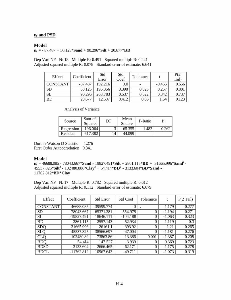
H-4
nf and PSD Model nf = - 87.487 + 50.125*Sand + 90.296*Silt + 20.677*BD Dep Var: NF N: 18 Multiple R: 0.491 Squared multiple R: 0.241 Adjusted squared multiple R: 0.078 Standard error of estimate: 6.641
Effect Coefficient Std Error
Std Coef Tolerance t P(2
Tail) CONSTANT -87.487 192.216 0.0 - -0.455 0.656 SD 50.125 195.356 0.398 0.023 0.257 0.801 SL 90.296 263.783 0.537 0.022 0.342 0.737 BD 20.677 12.607 0.412 0.86 1.64 0.123
Analysis of Variance
Source Sum-of-Squares DF Mean
Square F-Ratio P
Regression 196.064 3 65.355 1.482 0.262 Residual 617.382 14 44.099
Durbin-Watson D Statistic 1.276 First Order Autocorrelation 0.341 Model nf = 46688.085 - 78043.667*Sand - 19827.491*Silt + 2861.115*BD + 31665.996*Sand2 -45537.825*Silt2 - 102480.886*Clay2 + 54.414*BD2 - 3133.604*BD*Sand - 11762.812*BD*Clay Dep Var: NF N: 17 Multiple R: 0.782 Squared multiple R: 0.612 Adjusted squared multiple R: 0.112 Standard error of estimate: 6.679
Effect Coefficient Std Error Std Coef Tolerance t P(2 Tail)
CONSTANT 46688.085 39599.774 0 . 1.179 0.277 SD -78043.667 65371.381 -554.979 0 -1.194 0.271 SL -19827.491 18646.111 -104.188 0 -1.063 0.323 BD 2861.115 2557.143 52.934 0 1.119 0.3 SDQ 31665.996 26161.1 393.92 0 1.21 0.265 SLQ -45537.825 38566.697 -47.004 0 -1.181 0.276 CLQ -102480.89 73863.86 -13.386 0.001 -1.387 0.208 BDQ 54.414 147.527 3.939 0 0.369 0.723 BDSD -3133.604 2666.465 -62.171 0 -1.175 0.278 BDCL -11762.812 10967.643 -49.711 0 -1.073 0.319

H-5
Analysis of Variance
Source Sum-of-Squares DF
Mean Square F-Ratio P
Regression 491.846 9 54.65 1.225 0.403 Residual 312.242 7 44.606
Durbin-Watson D Statistic 2.052 First Order Autocorrelation -0.028 af and gradation indices (D60 and D10) Model af = 3.135 - 13.185*D10 + 0.219*D60 Dep Var: AF N: 18 Multiple R: 0.176 Squared multiple R: 0.031 Adjusted squared multiple R: 0.0 Standard error of estimate: 5.246
Effect Coefficient Std Error
Std Coef Tolerance t P(2
Tail) CONSTANT 3.135 2.775 0 . 1.13 0.276 DT -13.185 20.286 -0.182 0.822 -0.65 0.526 DS 0.219 0.441 0.139 0.822 0.496 0.627
Analysis of Variance
Source Sum-of-Squares DF Mean
Square F-Ratio P
Regression 13.273 2 6.636 0.241 0.789 Residual 412.813 15 27.521
Model af = -2.885 + 34.214*D10+ 4.669* D60 - 42.835*D102 + 0.212*D602 - 32.202*D10*D60 Dep Var: AF N: 18 Multiple R: 0.482 Squared multiple R: 0.232 Adjusted squared multiple R: 0.0 Standard error of estimate: 5.221
Effect Coefficient Std Error
Std Coef Tolerance t P(2
Tail) CONSTANT -2.885 6.539 0 . -0.441 0.667 DT 34.214 87.876 0.473 0.043 0.389 0.704 DS 4.669 2.654 2.969 0.022 1.759 0.104 DTQ -42.835 227.825 -0.199 0.057 -0.188 0.854 DSQ 0.212 0.334 1.546 0.011 0.634 0.538 DTDS -32.202 26.628 -4.614 0.004 -1.209 0.25

H-6
Analysis of Variance
Source Sum-of-Squares DF Mean
Square F-Ratio P
Regression 99.017 5 19.803 0.727 0.617 Residual 327.069 12 27.256
Durbin-Watson D Statistic 2.252 First Order Autocorrelation -0.151 hr and gradation indices (D60 and D10) Model hr = 13.728 - 24.081*D10 + 0.202*D60 Dep Var: HR N: 18 Multiple R: 0.123 Squared multiple R: 0.015 Adjusted squared multiple R: 0.0 Standard error of estimate: 12.963
Effect Coefficient Std Error
Std Coef Tolerance t P(2
Tail) CONSTANT 13.728 6.856 0 . 2.002 0.064 DT -24.081 50.125 -0.136 0.822 -0.48 0.638 DS 0.202 1.089 0.052 0.822 0.185 0.855
Analysis of Variance
Source Sum-of-Squares DF Mean
Square F-Ratio P
Regression 38.847 2 19.423 0.116 0.892 Residual 2520.48 15 168.032
Durbin-Watson D Statistic 1.693 First Order Autocorrelation 0.123 Model hr = - 8.797 + 215.863*D10 + 11.774*D60 - 428.641*D102 + 0.790*D602 - 96.776*D10*D60 Dep Var: HR N: 18 Multiple R: 0.509 Squared multiple R: 0.259 Adjusted squared multiple R: 0.0 Standard error of estimate: 12.569
Effect Coefficient Std Error
Std Coef Tolerance t P(2
Tail) CONSTANT -8.797 15.743 0 . -0.559 0.587 DT 215.863 211.563 1.217 0.043 1.02 0.328 DS 11.774 6.39 3.055 0.022 1.843 0.09 DTQ -428.641 548.496 -0.812 0.057 -0.781 0.45 DSQ 0.79 0.804 2.352 0.011 0.982 0.345 DTDS -96.776 64.109 -5.658 0.004 -1.51 0.157

H-7
Analysis of Variance
Source Sum-of-Squares DF Mean
Square F-Ratio P
Regression 663.559 5 132.712 0.84 0.546 Residual 1895.767 12 157.981
Durbin-Watson D Statistic 1.992 First Order Autocorrelation -0.030 mf and gradation indices (D60 and D10) Model mf = 0.198 + 2.411*D10 - 0.065*D60 Dep Var: MF N: 18 Multiple R: 0.747 Squared multiple R: 0.558 Adjusted squared multiple R: 0.499 Standard error of estimate: 0.193
Effect Coefficient Std Error Std Coef Tolerance t P(2 Tail) CONSTANT 0.198 0.102 0. 1.943 0.071DT 2.411 0.746 0.612 0.822 3.231 0.006DS -0.065 0.016 -0.759 0.822 -4.005 0.001
Analysis of Variance
Source Sum-of-Squares DF Mean
Square F-Ratio P
Regression 0.705 2 0.352 9.461 0.002 Residual 0.559 15 0.037
Durbin-Watson D Statistic 1.434 First Order Autocorrelation 0.238 Model mf = 0.318 + 1.351*D10 -0.113*D60 + 2.966*D102 + 0.005*D602 Dep Var: MF N: 18 Multiple R: 0.773 Squared multiple R: 0.597 Adjusted squared multiple R: 0.473 Standard error of estimate: 0.198
Effect Coefficient Std Error Std Coef Tolerance t P(2 Tail) CONSTANT 0.318 0.202 0. 1.574 0.139DT 1.351 2.869 0.343 0.058 0.471 0.646DS -0.113 0.055 -1.324 0.074 -2.042 0.062DTQ 2.966 8.349 0.253 0.061 0.355 0.728DSQ 0.005 0.005 0.614 0.075 0.958 0.356

H-8
Analysis of Variance
Source Sum-of-Squares DF Mean
Square F-Ratio P
Regression 0.754 4 0.189 4.817 0.013 Residual 0.509 13 0.039
Durbin-Watson D Statistic 1.286 First Order Autocorrelation 0.296 nf and gradation indices (D60 and D10) Model nf = 4.454 - 14.174*D10 + 1.200*D60 Dep Var: NF N: 18 Multiple R: 0.509 Squared multiple R: 0.259 Adjusted squared multiple R: 0.160 Standard error of estimate: 6.339
Effect Coefficient Std Error Std Coef Tolerance t P(2 Tail) CONSTANT 4.454 3.353 0. 1.328 0.204DT -14.174 24.513 -0.142 0.822 -0.578 0.572DS 1.2 0.533 0.552 0.822 2.252 0.04
Analysis of Variance
Source Sum-of-Squares DF Mean
Square F-Ratio P
Regression 210.66 2 105.33 2.621 0.106Residual 602.785 15 40.186
Durbin-Watson D Statistic 1.353 First Order Autocorrelation 0.314

H-9
Model nf = -1.636 + 66.995*D10 + 4.018*D60 -132.595*D102+ 0.503*D602 - 39.665*D10*D60 Dep Var: NF N: 18 Multiple R: 0.581 Squared multiple R: 0.338 Adjusted squared multiple R: 0.062 Standard error of estimate: 6.701
Effect Coefficient Std Error Std Coef Tolerance t P(2 Tail) CONSTANT -1.636 8.392 0. -0.195 0.849DT 66.995 112.784 0.67 0.043 0.594 0.564DS 4.018 3.406 1.849 0.022 1.179 0.261DTQ -132.595 292.401 -0.445 0.057 -0.453 0.658DSQ 0.503 0.429 2.656 0.011 1.173 0.264DTDS -39.665 34.176 -4.113 0.004 -1.161 0.268
Analysis of Variance
Source Sum-of-Squares DF Mean
Square F-Ratio P
Regression 274.684 5 54.937 1.224 0.356Residual 538.761 12 44.897
Durbin-Watson D Statistic 1.574 First Order Autocorrelation 0.203 af and gradation number CGN & FGN Model af = -4.189 + 2.871*CGN - 3.604*FGN Dep Var: AF N: 18 Multiple R: 0.204 Squared multiple R: 0.042 Adjusted squared multiple R: 0.0 Standard error of estimate: 5.218
Effect Coefficient Std Error
Std Coef Tolerance t P(2
Tail) CONSTANT -4.189 20.749 0 . -0.202 0.843 CGN 2.871 6.966 0.183 0.325 0.412 0.686 FGN -3.604 4.913 -0.325 0.325 -0.734 0.474
Analysis of Variance
Source Sum-of-Squares DF Mean
Square F-Ratio P
Regression 17.706 2 8.853 0.325 0.727 Residual 408.38 15 27.225
Durbin-Watson D Statistic 1.883 First Order Autocorrelation 0.052

H-10
Model af = 7.870 - 30.0*CGN + 79.167*FGN + 10.511*CGN2 + 19.729*FGN2 - 36.646*CGN x FGN Dep Var: AF N: 18 Multiple R: 0.353 Squared multiple R: 0.125 Adjusted squared multiple R: 0.0 Standard error of estimate: 5.575
Effect Coeffic ient Std Error
Std Coef Tolerance t P(2
Tail) CONSTANT 7.87 256.815 0 . 0.031 0.976 CGN -30 185.208 -1.91 0.001 -0.162 0.874 FGN 79.167 159.191 7.148 0 0.497 0.628 CGNSQ 10.511 34.858 4.638 0 0.302 0.768 FGNSQ 19.729 23.701 4.987 0.002 0.832 0.421 CFGN -36.646 58.192 -14.64 0 -0.63 0.541
Analysis of Variance
Source Sum-of-Squares DF Mean
Square F-Ratio P
Regression 53.145 5 10.629 0.342 0.878 Residual 372.941 12 31.078
Durbin-Watson D Statistic 2.008 First Order Autocorrelation -0.010 nf and gradation number CGN & FGN Model nf = 21.653 - 2.766*CGN - 5.126*FGN Dep Var: NF N: 18 Multiple R: 0.446 Squared multiple R: 0.199 Adjusted squared multiple R: 0.092 Standard error of estimate: 6.592
Effect Coefficient Std
Error Std
Coef Tolerance t P(2 Tail)
CONSTANT 21.653 26.214 0 . 0.826 0.422 CGN -2.766 8.801 -0.127 0.325 -0.314 0.758 FGN -5.126 6.207 -0.335 0.325 -0.826 0.422
Analysis of Variance
Source Sum-of-Squares DF
Mean Square F-Ratio P
Regression 161.562 2 80.781 1.859 0.19 Residual 651.883 15 43.459
Durbin-Watson D Statistic 1.540 First Order Autocorrelation 0.210

H-11
Model nf = -243.818 + 209.641*CGN - 203.247*FGN - 38.388*CGN2 - 4.062*FGN2 + 55.604 *CGN x FGN Dep Var: NF N: 18 Multiple R: 0.643 Squared multiple R: 0.414 Adjusted squared multiple R: 0.169 Standard error of estimate: 6.305
Effect Coefficient Std Error
Std Coef Tolerance t P(2
Tail) CONSTANT -243.818 290.455 0 . -0.839 0.418 CGN 209.641 209.468 9.66 0.001 1.001 0.337 FGN -203.247 180.044 -13.281 0 -1.129 0.281 CGNSQ -38.388 39.425 -12.259 0 -0.974 0.349 FGNSQ -4.062 26.805 -0.743 0.002 -0.152 0.882 CFGN 55.604 65.815 16.076 0 0.845 0.415
Analysis of Variance
Source Sum-of-Squares DF Mean
Square F-Ratio P
Regression 336.404 5 67.281 1.692 0.211 Residual 477.041 12 39.753
Durbin-Watson D Statistic 1.827 First Order Autocorrelation 0.062 mf and gradation number CGN & FGN Model mf = -0.871 + 0.305*CGN + 0.109*FGN Dep Var: MF N: 18 Multiple R: 0.515 Squared multiple R: 0.266 Adjusted squared multiple R: 0.168 Standard error of estimate: 0.249
Effect Coefficient Std Error
Std Coef Tolerance t P(2
Tail) CONSTANT -0.871 0.989 0 . -0.881 0.392 CGN 0.305 0.332 0.357 0.325 0.92 0.372 FGN 0.109 0.234 0.18 0.325 0.464 0.649
Analysis of Variance
Source Sum-of-Squares DF Mean
Square F-Ratio P
Regression 0.335 2 0.168 2.712 0.099 Residual 0.928 15 0.062
Durbin-Watson D Statistic 2.014 First Order Autocorrelation -0.059

H-12
Model mf = 5.912 - 4.935*CGN + 4.055*FGN + 0.974*CGN2 + 0.361*FGN2 - 1.348*CGN x FGN Dep Var: MF N: 18 Multiple R: 0.544 Squared multiple R: 0.296 Adjusted squared multiple R: 0.002 Standard error of estimate: 0.272
Effect Coefficient Std Error
Std Coef Tolerance t P(2
Tail) CONSTANT 5.912 12.544 0 . 0.471 0.646 CGN -4.935 9.047 -5.77 0.001 -0.545 0.595 FGN 4.055 7.776 6.723 0 0.521 0.612 CGNSQ 0.974 1.703 7.897 0 0.572 0.578 FGNSQ 0.361 1.158 1.678 0.002 0.312 0.76 CFGN -1.348 2.842 -9.888 0 -0.474 0.644
Analysis of Variance
Source Sum-of-Squares DF Mean
Square F-Ratio P
Regression 0.373 5 0.075 1.007 0.455 Residual 0.89 12 0.074
Durbin-Watson D Statistic 2.067 First Order Autocorrelation -0.086 hr and gradation number CGN & FGN Model hr = 7.633 + 2.349*CGN - 4.291*FGN Dep Var: HR N: 18 Multiple R: 0.113 Squared multiple R: 0.013 Adjusted squared multiple R: 0.0 Standard error of estimate: 12.978
Effect Coefficient Std Error
Std Coef Tolerance t P(2
Tail) CONSTANT 7.633 51.607 0 . 0.148 0.884 CGN 2.349 17.327 0.061 0.325 0.136 0.894 FGN -4.291 12.219 -0.158 0.325 -0.351 0.73
Analysis of Variance
Source Sum-of-Squares DF Mean
Square F-Ratio P
Regression 32.91 2 16.455 0.098 0.907 Residual 2526.416 15 168.428
Durbin-Watson D Statistic 1.679 First Order Autocorrelation 0.126

H-13
Model hr = -300.842 + 135.324*CGN + 210.770*FGN - 11.963*CGN2 + 24.338*FGN2 - 70.121*CGN x FGN Dep Var: HR N: 18 Multiple R: 0.313 Squared multiple R: 0.098 Adjusted squared multiple R: 0.0 Standard error of estimate: 13.869
Effect Coefficient Std
Error Std
Coef Tolerance t P(2 Tail)
CONSTANT -300.842 638.884 0 . -0.471 0.646 CGN 135.324 460.745 3.515 0.001 0.294 0.774 FGN 210.77 396.023 7.764 0 0.532 0.604 CGNSQ -11.963 86.718 -2.154 0 -0.138 0.893 FGNSQ 24.338 58.961 2.51 0.002 0.413 0.687 CFGN -70.121 144.766 -11.43 0 -0.484 0.637
Analysis of Variance
Source Sum-of-Squares DF
Mean Square F-Ratio P
Regression 251.293 5 50.259 0.261 0.926 Residual 2308.034 12 192.336
Durbin-Watson D Statistic 1.909