research techniques in animal ecology - luigi boitani
TRANSCRIPT

Research Techniques in Animal Ecology
Methods and Cases in Conservation Science
Mary C. Pearl, Editor

Methods and Cases in Conservation Science
Tropical Deforestation: Small Farmers and Land Clearing in the Ecuadorian AmazonThomas K. Rudel and Bruce Horowitz
Bison: Mating and Conservation in Small PopulationsJoel Berger and Carol Cunningham,
Population Management for Survival and Recovery: Analytical Methods and Strategies inSmall Population ConservationJonathan D. Ballou, Michael Gilpin, and Thomas J. Foose,
Conserving Wildlife: International Education and Communication ApproachesSusan K. Jacobson
Remote Sensing Imagery for Natural Resources Management: A First Time User’s GuideDavid S. Wilkie and John T. Finn
At the End of the Rainbow? Gold, Land, and People in the Brazilian AmazonGordon MacMillan
Perspectives in Biological Diversity Series
Conserving Natural ValueHolmes Rolston III
Series Editor, Mary C. Pearl
Series Advisers, Christine Padoch and Douglas Daly

Research Techniques in Animal Ecology
Controversies and Consequences
Luigi Boitani and Todd K. FullerEditors
C
COLUMBIA UN IVERS ITY PRESS
NEW YORK

Columbia University PressPublishers Since 1893New York Chichester, West Sussex
Copyright © 2000 by Columbia University PressAll rights reservedLibrary of Congress Cataloging-in-Publication Data
Research techniques in animal ecology : controversies and consequences / Luigi Boitaniand Todd K. Fuller, editors.
p. cm. — (Methods and cases in conservation science)Includes bibliographical references (p. ).ISBN 0–231–11340–4 (cloth : alk. paper)—ISBN 0–231–11341–2 (paper : alk. paper)1. Animal ecology—Research—Methodology. I. Boitani, Luigi. II. Fuller, T. K. III.
Series.
QH541.2.R47 2000591.7′07′2—dc21 99–052230
`
Casebound editions of Columbia University Press books are printed on permanent anddurable acid-free paper.Printed in the United States of Americac 10 9 8 7 6 5 4 3 2 1p 10 9 8 7 6 5 4 3 2 1

ForStefania and CaterinaandSusan and Molliefor their patience, love, and support


Contents
authors xvlist of illustrations xixlist of tables xxiiipreface xxv
Chapter 1: Hypothesis Testing in EcologyCharles J. Krebs 1
Some Definitions 1What Is a Hypothesis? 3Hypotheses and Models 4Hypotheses and Paradigms 6Statistical Hypotheses 8Hypotheses and Prediction 10Acknowledgments 12Literature Cited 12
Chapter 2: A Critical Review of the Effects of Marking on theBiology of VertebratesDennis L. Murray and Mark R. Fuller 15
Review of the Literature 16Which Markers to Use? 17Effects of Markers Among Taxa 17Critique of Marker Evaluation Studies 35Review of Current Guidance Available for Choosing Markers 37Critique of Guidelines Available for Choosing Markers 39

viii CONTENTS
Survey of Recent Ecological Studies 40Future Approaches 42
Study Protocols and Technological Advances 43Marker Evaluation Studies 44
Acknowledgments 46Literature Cited 46
Chapter 3: Animal Home Ranges and Territories and Home Range EstimatorsRoger A. Powell 65
Definition of Home Range 65Territories 70Estimating Animals’ Home Ranges 74
Utility Distributions 75Grids 77Minimum Convex Polygon 79Circle and Ellipse Approaches 80Fourier Series 80Harmonic Mean Distribution 81Fractal Estimators 82Kernel Estimators 86Home Range Core 91
Quantifying Home Range Overlap and Territoriality 94Static Interactions 95Dynamic Interactions 97Testing for Territoriality 98
Lessons 100Acknowledgments 103Literature Cited 103
Chapter 4: Delusions in Habitat Evaluation: Measuring Use,Selection, and ImportanceDavid L. Garshelis 111
Terminology 112Methods for Evaluating Habitat Selection, Preference, and Quality 114
Use–Availability Design 114Site Attribute Design 117Demographic Response Design 118
Problems with Use–Availability and Site Attribute Designs 118

Defining Habitats 118Measuring Habitat Use 120Measuring Habitat Availability 122Assessing Habitat Selection: Fatal Flaw 1 127Inferring Habitat Quality: Fatal Flaw 2 139
Advantages and Problems of the Demographic Response Design 144Applications and Recommendations 147Acknowledgments 153Literature Cited 153
Chapter 5: Investigating Food Habits of Terrestrial VertebratesJohn A. Litvaitis 165
Conventional Approaches and Their Limitations 166Direct Observation 166Lead Animals 167Feeding Site Surveys 167Exclosures 170Postingestion Samples 170
Evaluating the Importance of Specific Foods and Prey 175Use, Selection, or Preference? 175Availability Versus Abundance 175Cafeteria Experiments 176
Innovations 176Improvements on Lead Animal Studies 176Use of Isotope Ratios 177Experimental Manipulations 177The Role of Foraging Theory in Understanding Food Habits 179
Lessons 181Sample Resolution and Information Obtained 181Improving Sample Resolution and Information Content 182
Literature Cited 183
Chapter 6: Detecting Stability and Causes of Change in Population DensityJoseph S. Elkinton 191
Detection of Density Dependence 193Analysis of Time Series of Density 193Analysis of Data on Mortality or Survival 196
Detection of Delayed Density Dependence 199
CONTENTS ix

x CONTENTS
Detection of Causes of Population Change 201Key Factor Analysis 201
Experimental Manipulation 205Conclusions 208Literature Cited 209
Chapter 7: Monitoring PopulationsJames P. Gibbs 213
Index–Abundance Relationships 214Types of Indices 214Index–Abundance Functions 215Variability of Index–Abundance Functions 217Improving Index Surveys 220
Spatial Aspects of Measuring Changes in Indices 221Monitoring Indices Over Time 222
Power Estimation for Monitoring Programs 223Variability of Indices of Animal Abundance 224Sampling Requirements for Robust Monitoring Programs 227Setting Objectives for a Monitoring Program 228
Conclusions 229Acknowledgments 232Appendix 7.1 233Literature Cited 247
Chapter 8: Modeling Predator–Prey DynamicsMark S. Boyce 253
Modeling Approaches for Predator–Prey Systems 254Noninteractive Models 255True Predator–Prey Models 260Stochastic Models 269Autoregressive Models 270
Fitting the Model to Data 273Bayesian Statistics 273Best Guess Followed by Adaptive Management 273
Choosing a Good Model 275How Much Detail? 275Model Validation 277
Recommendations 279Remember the Audience 279

Conclusion 281Acknowledgments 281Literature Cited 282
Chapter 9: Population Viability Analysis: Data Requirements andEssential AnalysesGary C. White 288
Qualitative Observations About Population Persistence 290Generalities 290Contradictions 292
Sources of Variation Affecting Population Persistence 293No Variation 293Stochastic Variation 293Demographic Variation 295Temporal Variation 297Spatial Variation 300Individual Variation 300Process Variation 303
Components of a PVA 303Direct Estimation of Variance Components 305Indirect Estimation of Variance Components 312Bootstrap Approach 313Basic Population Model and Density Dependence 314Incorporation of Parameter Uncertainty into Persistence Estimates 319Discussion 322Conclusion 325Literature Cited 327
Chapter 10: Measuring the Dynamics of Mammalian Societies: An Ecologist’s Guide to Ethological MethodsDavid W. Macdonald, Paul D. Stewart, Pavel Stopka, and Nobuyuki Yamaguchi 332
Social Dynamics 332Context 334Why Study Social Dynamics? 335
Evolution of Sociality 335Conservation Applications 335Understanding Ourselves 336
How to Describe Social Dynamics 337
CONTENTS xi

xii CONTENTS
Action, Interaction, and Relationships 337Social Networks 338Social Structure, from Surface to Deep 339
Behavioral Parameters 340The Bout 340Stationarity 343The Ethogram 343Beware Teleology 345Classifications of Behavioral Interactions 347
Methods for Behavioral Measurement 362Identifying the Individual 362Sampling and Recording Rules 364Ad Libitum Sampling 365Focal Sampling 365Time Sampling 366Techniques for Behavioral Measurement 368
Analysis of Observational Data 369Statistical Rationality 370Matrix Facilities: Analyzing Sequential Data 371Lag Sequential and Nested Analysis 374Searching for a Behavioral Pattern (Markov Chain) 375Predictability of Behavior 376Sequences Through the Mist 378
Acknowledgments 380Literature Cited 380
Chapter 11: Modeling Species Distribution with GISFabio Corsi, Jan de Leeuw, and Andrew K. Skidmore 389
Terminology 391Habitat Definitions and Use 392General Structure of GIS-Based Models 396
Literature Review 401Modeling Issues 403
Clear Objectives 403Assumptions 405Spatial and Temporal Scale 408Data Availability 412Validation and Accuracy Assessment 413

Discussion 422Conclusions 424Acknowledgments 425Notes 425Literature Cited 426
index 435
CONTENTS xiii


Authors
Luigi BoitaniDipartimento Biologia Animale dell’UomoUniversità di Roma “La Sapienza”Viale Università 3200185 Rome, Italy
Mark S. BoyceDepartment of Biological SciencesUniversity of AlbertaEdmonton, Alberta T6G 2E9, Canada
Fabio CorsiInstitute of Applied Ecology (IAE)Via L. Spallanzani 3200161 Rome, Italy
Joseph S. ElkintonDepartment of Entomology and Graduate Program in Organismic
and Evolutionary BiologyUniversity of MassachusettsAmherst, MA 01003, USA

xvi AUTHORS
Mark R. FullerUSGS Forest and Rangeland Ecosystem Science CenterSnake River Field Station
and Boise State University970 Lusk StreetBoise, ID 83706, USA
Todd K. FullerDepartment of Natural Resources Conservation and Graduate
Program in Organismic and Evolutionary BiologyUniversity of MassachusettsAmherst, MA 01003-4210, USA
David L. GarshelisMinnesota Department of Natural Resources1201 E. Highway 2Grand Rapids, MN 55744, USA
James P. GibbsState University of New YorkCollege of Environmental Science and ForestryFaculty of Environmental and Forest Biology350 Illick Hall, 1 Forestry DriveSyracuse, NY 13210, USA
Charles J. KrebsDepartment of ZoologyUniversity of British Columbia6270 University Blvd.Vancouver, BC V6T 1Z4, Canada
Jan de LeeuwDivision of Agriculture, Conservation, and the EnvironmentInternational Institute for Aerospace SurveyP.O. Box 67500 AA Enschede, The Netherlands

John A. LitvaitisDepartment of Natural ResourcesUniversity of New HampshireDurham, NH 03824, USA
David W. MacdonaldWildlife Conservation Research UnitDepartment of ZoologyUniversity of OxfordSouth Parks RoadOxford OX1 3PS, UK
Dennis L. MurrayDepartment of Fish and Wildlife ResourcesUniversity of IdahoMoscow, ID 83844, USA
Roger A. PowellDepartment of ZoologyNorth Carolina State UniversityRaleigh, NC 27695-7617, USA
Andrew SkidmoreDivision of Agriculture, Conservation, and the EnvironmentInternational Institute for Aerospace SurveyP.O. Box 67500 AA Enschede, The Netherlands
Paul D. StewartWildlife Conservation Research UnitDepartment of ZoologyUniversity of OxfordSouth Parks RoadOxford OX1 3PS, UK
Pavel StopkaWildlife Conservation Research UnitDepartment of ZoologyUniversity of OxfordSouth Parks RoadOxford OX1 3PS, UK
AUTHORS xvii

xviii AUTHORS
Gary C. WhiteDepartment of Fishery and Wildlife BiologyColorado State UniversityFort Collins, CO 80523, USA
Nobuyuki YamaguchiWildlife Conservation Research UnitDepartment of ZoologyUniversity of OxfordSouth Parks RoadOxford OX1 3PS, UK

List of Illustrations
1.1 Classic illustration of the density-dependent paradigm of populationregulation
3.1 Location estimates for adult female bear 61 in the Pisgah Bear Sanctu-ary, North Carolina
3.2 Location estimates and contours for the probability density functionfor adult female black bear 87
3.3 Locations of (a) an adult female black bear, (b) an adult wolf, and (c)an adult male stone marten
3.4 A complex, simulated home range3.5 The 95% fixed kernel home range for adult female black bear 61 in
19833.6 Possible relationships between probability of use and percentage of
home range3.7 Core area and home range for an adult female bear4.1 Hypothetical movements of an animal overlaid on five habitat types4.2 Hypothetical relationships between area and use of habitat4.3 The assumed linear relationship between use and availability of
resources4.4 The assumed linear relationship between use and availability of habi-
tats5.1 Comparison of four methods used to investigate prey use by wolves5.2 Relationship between 13C signatures of the diet of equilibrated plasma
in black bears and polar bears5.3 Relationship between 15N signatures of the diet of equilibrated plasma
in black bears and polar bears

xx I LLUSTRAT IONS
5.4 Internal and external factors affecting foraging decisions by a lago-morph
5.5 Information content and sample resolution of common methods usedto investigate vertebrate food habits
6.1 Change in gypsy moth density6.2 (a) Percentage mortality of gypsy moth, and (b) time series of percent-
age mortality of gypsy moth6.3 Graphic detection of delayed density dependence6.4 Use of time series to detect delayed density dependence6.5 Key factor analysis of a population of the partridge Perdix perdix L. in
England7.1 Relationship between population indices and actual animal abundance7.2 Variation between habitats in index–abundance relationships7.3 Variation in the index–abundance relationship over time8.1 Graphic representation of a single-species model for prey abundance8.2 Stable-limit cycle from a two-species predator–prey model8.3 Illustrations of hypothetical type I, II, and III functional responses for
wolves preying on elk8.4 Functional and numerical responses for wolves preying on moose8.5 Stability map for a second-order autoregressive process8.6 Population dynamics emerging from second-order autoregressive mod-
els9.1 Deterministic model of population growth9.2 Three examples of the outcome of the population model with only
demographic variation9.3 Persistence of a population as a function of initial population size9.4 Examples of the beta distribution, all with mean 0.59.5 Persistence of a population of 100 animals at t = 0 to t = 100 years9.6 Effect of individual variation on population persistence9.7 Three examples of possible relationships of recruitment per individual
to population size9.8 Example of how an Allee effect is created by a declining birth rate at
low densities10.1 Data on the interactions between male and female wood mice10.2 The proportion of time spent grooming different portions of the body
surface10.3 Barplots of badger allogrooming behavior10.4 What constitutes proximity between individuals differs between
species

10.5 Considerations in scoring indices of association10.6 Exploration of patterns of spatial proximity10.7 The goal of translating indices of social behavior into evolutionary
consequences10.8 The same observations of social interactions expressed in three ways10.9 The flow of rubbing between a group of four cats10.10 The flow diagram (state-space representation) of the sex-dependent
nose-to-nose interaction11.1 Percentage of papers dealing with habitat modeling11.2 General data flow of the two main categories of GIS species distribu-
tion models identified11.3 Population dynamics event in relation to time and space scales
I LLUSTRAT IONS xxi


List of Tables
2.1 Survey of marker evaluation studies in fish2.2 Survey of marker evaluation studies in reptiles and amphibians2.3 Survey of marker evaluation studies in birds2.4 Survey of marker evaluation studies in mammals2.5 Review of treatment of potential marking effects in the ecological liter-
ature3.1 Simple probability index for home range overlap of adult female black
bears, wolves and wolf packs, and stone martens4.1 Effect of habitat availability on perceived selection4.2 Effect of altered availability (floor space) on perceived selection of
rooms in a house4.3 Habitat use, availability, and perceived selection for Gaur and Banteng
in Thailand during the dry season5.1 Evaluation of methods used to investigate vertebrate food habits5.2 Application of digestion correction factors (CF) used to estimate the
biomass7.1 Monte Carlo simulation procedure used to estimate the power of pop-
ulation-monitoring programs to detect trends7.2 Variability estimates for local populations7.3 Sampling intensities needed to detect overall population changes10.1 Matrix of frequencies of transitions from fight to avoidance and fre-
quencies of allogrooming behavior among nine wood mice11.1 Classification scheme of the term habitat11.2 Classification of reviewed papers11.3 Typical error matrix


Preface
As science, ecology is often accused of being weak because of its basic lack ofpredictive power (Peters 1991) and the many ecological concepts judged vagueor tautological (Shrader-Frechette and McCoy 1993). Also, important para-digms that dominated the ecological scene for years have been discarded infavor of new concepts and theories that swamp the most recent ecologicalliterature (e.g., the abandoning of the island biogeography theory in favor ofthe metapopulations theory; Hanski and Simberloff 1997). The apparent easewith which such changes seem to be accepted could be taken as an intrinsicweakness of ecological disciplines; in fact, many ecologists seem to have an infe-riority complex with respect to sciences considered more rigorous, such as physics or chemistry. Thus, when ecology has to provide the basis for envi-ronmental conservation and management, this presumed weakness is easilyinstrumentalized by those opposing conservation. In the often sterile debatesthat are heard, ecology loses credibility and is easily victimized by its detractors.
It is not surprising that many ecological theories and concepts have still notbeen defined precisely, given the enormous complexity of ecological systems.Yet ecology is rooted in the scientific method applied to the observation andexperimentation of natural facts. Rather than a discipline whose experimentalpractice is informed by laws and invincible paradigms, ecology is a classicallybottom-up discipline in which the application of the scientific method to realfacts and processes gradually builds a body of knowledge that can give rise touseful generalizations. But the complexity of ecological processes and theirvariability is such that any generalization conflicts with the need to account forall possible variations. It is in this light that the rigor of the results achieved inthe study of real cases takes on fundamental value. Without embracing such

xxvi PREFACE
radically critical positions as those summarized by Shrader-Frechette andMcCoy (1993), we nevertheless feel that ecology, like any other discipline inthe natural sciences, can only benefit from the steadily growing scientific rigorin the study of real cases.
Animal ecology, in particular, is the field in which we should strive formore scrupulous application of a scientifically rigorous methodology. Animalpopulations are mobile in space, they have a strong stochastic demographiccomponent, they are involved in complex interspecific and intraspecific inter-actions and interactions with the abiotic environment, and they have a greatenvironmental variance. Thus it has been more difficult to apply scientificapproaches and rigorous experimental designs to them than in other scientificendeavors. Nonetheless, there is no good justification for studying animal pop-ulations without greater discipline.
These intrinsic difficulties in studying animal ecology underlie many of theweaknesses in the research methodologies available to researchers today. Cer-tainly the quality of the research is sometimes limited by logistic and environ-mental adversities, by the problems of translating into practice an experimen-tal design worked out at the drawing board, by deliberately limited samples,and by other problems that can contribute to weakening the methodologicalrigor of a study and therefore the validity of its results. As the methods andresults of animal ecology are often applied to conservation, the practical con-sequences of misused techniques can mislead the implementation of conserva-tion measures. For many species, such mistakes can have serious consequences.
This book springs from the recurring frustration we, the editors, some-times have felt while doing our work as researchers and teachers. The scientificecological literature (as well as a good bit of other literature) is full of publica-tions based on false assumptions and methodological errors. Although thenumber of methodological errors and omissions seems to be inversely andexponentially proportional to a journal’s quality, even the most scrupulous edi-tors of the best scientific journals sometimes miss mistakes. Although the mostcircumspect researchers have the critical ability to recognize and respond to theerrors, often they do not respond, and such critique is almost totally absentamong students. Teaching students how to be critical is perhaps the most dif-ficult and most noble objective of the teaching profession, but there has neverbeen a text in the field of animal ecology to help us in this task. Excellent hand-books and textbooks of techniques and methods are available (e.g., Krebs1999; Bookhout 1994) in which the techniques are well described and exam-ples are used to illustrate when and how to apply them. Many of these tech-niques are well known and robust in their applications. However, several

require assumptions and procedures that are not always accounted for. Con-ceptual limitations and methodological constraints are not often discussed inthe scientific literature, and currently there are no other books from which onecan learn a critical approach to use of the wide variety of methods and tech-niques in animal ecology.
The main purpose of this book, therefore, is to present some of the morecommon issues and research techniques used in animal ecology, identify theirlimitations and most common misuses, provide possible solutions, and addressthe most interesting new perspectives on how best to analyze and interpretdata collected in a variety of research areas. It is not a handbook of techniques;rather, it is designed as a backup for existing handbooks, providing a criticalperspective on the most common topics and techniques.
Such a critical review of methodologies is rare in animal ecology. Histori-cally, a few individual papers have denounced misused techniques, and suchpapers are still cited today. Others have had to be published several timesbefore the scientific community has taken notice. In recent years, individualpapers have been discussed in some journals via a comment and reply format,and these “conversations” are among the most interesting parts of those publi-cations. Several summarizing monographs or books have been publishedrecently that critically address or review major topics (e.g., radiotelemetry,population estimation, survival analyses), but no single volume has presenteda whole range of topics relevant to animal ecology.
In the course of the last 20 years of teaching, research, and editing, we have become increasingly convinced of the need for a book like this, with itscritical look at how ecological research is conducted and interpreted, and wehope it will provide insight and reassurance for the research community.Furthermore, we hope the book, by specifically investigating the many ways in which research techniques are incorrectly applied, will contribute to in-creasing the consistency and reliability of the scientific method in ecology andconservation.
The book includes the topics that are most frequently reported in the sci-entific literature in ecology and conservation, but rarely critically reviewed in acomprehensive manner. We are aware that several other topics and extensivetreatment of taxa other than vertebrates could have been included if there hadbeen no limitations on size and readability. We prepared a priority scale of top-ics based on the relevance of the issue, the lack of good available critical review,the availability of outstanding contributors, and the amount of controversyand misuse found on each topic. The resulting choice is obviously subjectiveand can be criticized, as every scientist has his or her preferences and perspec-
PREFACE xxvii

xxviii PREFACE
tives. However, we are confident that the book will address new topics of inter-est to a large proportion of researchers in animal ecology.
Each chapter explores and develops a different topic and includes an exten-sive review of published material and a summary of the state of knowledge onthat particular topic. Techniques are usually described only briefly because theintent is to point out the underlying assumptions and constraints of the tech-niques and indicate ways to avoid the most common pitfalls that await us.
In the first chapter Charles Krebs presents the philosophical groundworkconcerning hypotheses. He then discusses how this concept is translated in sci-entific studies into testable hypotheses, and then into statistical hypothesesand all of the attending problems that the simple idea of null hypotheses raises.He then explores the practical problems of hypothesis testing in ecology.Despite the fact that most ecologists and students in ecology think that goodhypothesis development is self-evident to any rational person, Krebs makes aconvincing case that the intellectual baggage of assumptions we all carry oughtto be questioned seriously.
Marking individual animals is often a prerequisite of many research designsin animal ecology. Although most ecologists are aware that some markers mayaffect an animal’s life history, this topic is rarely addressed in presentingresearch results. In chapter 2, Dennis L. Murray and Mark R. Fuller review theeffects of markers on various aspects of life history, particularly on movementsand energetics, and on survival and population estimation. They provide use-ful information on methodological or analytical modifications used to mini-mize the effects of markers and suggest lines of research to more fully evaluatethe effects of markers on various vertebrate taxa.
The concept of home range is central to much of the animal distributionand abundance literature, and home range descriptors have received muchcritical attention. Nevertheless, assumptions and caveats often are ignored,especially when the most modern techniques are used. Whereas the method-ological literature appears to cover extensively all critical aspects of this topic,the literature concerning the use of these methods does not reflect the samelevel of attention. Roger A. Powell, in chapter 3, analyzes old and recent pit-falls of home range and territory concepts and methods, and suggests the mostreliable approaches for each research theme.
The evaluation of habitat use by an animal either for use, preference, andselection studies or for suitability analyses is also a theme that is found easily inany current issue of the most important journals in animal ecology. However,the topic is full of delusions, as explained by David L. Garshelis in chapter 4.There are problems in defining and measuring habitats, measuring what is

really available to an animal, and assessing whether and what selection is even-tually made by an individual. Adequately addressing the assumptions thatform the basis of habitat selection hypotheses proves to be a formidableresearch design task. Equally challenging are problems with assessing habitatquality, including the basic concept of optimal habitat and the sometimes falseparadigm that the best habitat always supports higher animal densities.
In chapter 5 John A. Litvaitis summarizes the current approaches anddescribes the most recent innovations to investigating food habits and diets.The limitations of each technique are discussed but the emphasis is on theinterpretation of the results provided by these techniques. A number of funda-mental assumptions are neglected far too often when extrapolating individualresults to whole populations, and inadequate consideration of the spatiotem-poral variance of populations is common. Litvaitis also suggests framing habi-tat and food use studies within an integrated approach and shows the poten-tial of foraging theory as an aid in understanding variation in food habits.
Detection of time series of density and survival is the focus of chapter 6, byJoseph S. Elkinton. Understanding the mechanism by which populationdynamics develop is of paramount importance for conservation and manage-ment, and this chapter discusses the use of density and mortality data todeduce population changes and their causes. Density dependence is an espe-cially important parameter that is difficult to isolate from correlated factors,and Elkinton explores the statistical limitations of research design in detectingdifferent types of density dependence.
Population monitoring is a key topic in animal ecology and in mostwildlife conservation activities. However, James P. Gibbs, in chapter 7, showsthat the validity of the chosen population index is rarely assessed properly andthe design of a monitoring program usually is not adequate to permit a rea-sonable chance of detecting a trend or change. Gibbs discusses the many weak-nesses and limitations of population indexes and shows how imprecise popu-lation indices often combine with inadequate study design (often imposed bylogistical constraints) to severely constrain the statistical power of population-monitoring programs. After a thorough examination of the most common pit-falls of population monitoring, Gibbs points out the possible solutions. Thegoals set out clearly before the initiation of any monitoring program should, ata minimum, address the magnitude of change in the population index thatmust be detected, what probability of false detections is to be tolerated, andwhat frequency of failed detections is acceptable.
In chapter 8, Mark S. Boyce presents various types of predator–prey mod-els used in ecological research and discusses the criteria by which a model is
PREFACE xxix

xxx PREFACE
found to be good and useful. He identifies the conceptual limitations andpractical constraints of old and new approaches, whether from the Lotka–Volterra model or recent structured population models. Boyce carefully ana-lyzes the ways model are or can be validated, a necessary step in making a use-ful model, and he develops the need for adaptive management, where modelsplay a role that is strictly integrated into the monitoring of model predictions.
Population viability analyses (pvas) have become one of the most populartechniques used to assess conservation options for small populations. Severaltools have been developed to carry out such analyses, but despite their greatimportance in conservation biology, Gary C. White, in chapter 9, discusseswhy the current techniques are largely unsatisfactory. He identifies the weak-nesses of most estimates of population viability and points out the basic fail-ures of most models: their inability to account for individual variation withinthe population and for life-long individual heterogeneity. White also exploresother aspects of current PVA methods and shows that, as they stand, they areoften useless for conservation purposes. White’s critical approach is a powerfulwarning against the use of PVA results for practical conservation, but also showsthe potential role of improved PVA models as research tools for understandingthe dynamics of small populations.
Ethological aspects underlie many ecological studies of animals, and eventhough the two disciplines refer to two different theoretical and methodologi-cal frameworks, ecologists must become familiar with behavioral methods. Inchapter 10, David W. Macdonald, Paul D. Stewart, Pavel Stopka, andNobuyuki Yamaguchi provide a short guide to the main problems of measur-ing the dynamics of mammal societies. The greater emphasis is on socialbehavior, with particular attention to the many new concepts in behavioralecology, together with the refinement of sequential statistical techniques and,very importantly, the development of many software packages to facilitate thedescription of social dynamics. The chapter develops the identification of thesocial parameters that one might choose to define the social dynamics of mam-mal societies, the description of the methods used to record the most impor-tant parameters, and an introduction to the style of quantitative ethologicalanalyses currently in vogue (e.g., lag sequential analysis and multiple-matrixanalysis). The chapter ends by proposing a new conceptual framework forinterpreting data and asking whether parallels in the development of ecologi-cal communities and animal societies are merely analogies or evidence of sim-ilar underlying processes.
The final chapter, by Fabio Corsi, Jan de Leeuw, and Andrew Skidmore,presents state-of-the-art uses of geographic information systems (GISs) in thestudy of species distribution. Although the GIS is a fairly new and attractive tool

that can produce a completely new set of results unavailable until few yearsago, the authors warn against many conceptual limitations and potentialsources of error. In particular, the chapter analyzes the growth and misuse ofthe concept of habitat, with its many different meanings in biological andmapping sciences; these include habitat as a multidimensional species-specificproperty and habitat as a Cartesian property of land. The authors discuss theaccuracy of spatial wildlife habitat models, the dichotomy of inductive versusdeductive modeling, and the problem of transferability of models in space andtime. Finally, they warn us of the fundamental problem of scale dependency ofthe habitat factors and provide a set of procedures on error assessment.
This book is the result of a workshop that was held at the Ettore MajoranaCentre for Scientific Culture in Erice, Sicily, from November 28 to December3, 1996, which brought together a small number of highly qualified scientistsfor a 4-day discussion with a selected audience of 75 students, faculty, and sci-entists. Many people helped to make the workshop a success. First, we wish tothank Professor Danilo Mainardi, director of the International School ofEthology of the Ettore Majorana Centre for Scientific Culture for his insightand support in getting the project approved and funded by the Centre. We alsowish to thank Marco Lambertini for his participation in organizing the work-shop and the excellent staff of the center for making life in Erice a memorableevent. Each manuscript was reviewed by at least two external experts in thevarious topic areas and we especially thank our group of 24 anonymous refer-ees for their time and effort, which resulted in a much-improved book. Wewould also like to thank Ed Lugenbeel, Holly Hodder, and Roy Thomas ofColumbia University Press for encouraging the publication of the book andfor editorial assistance, Carol Anne Peschke for editorial skills providedthroughout the editing and publication process, and Ilaria Marzetti whohelped prepare the index.
Luigi BoitaniDepartment of Animal and Human BiologyUniversity of Rome “La Sapienza”
Todd K. FullerDepartment of Natural Resources ConservationUniversity of Massachusetts, Amherst
Literature Cited
Bookhout, T. A., ed. 1994. Research and management techniques for wildlife and habitats.Bethesda, Md.: The Wildlife Society.
PREFACE xxxi

xxxii PREFACE
Hanski, I. and D. Simberloff. 1997. The metapopulation approach, its history, conceptualdomain, and application to conservation. In I. Hanski and M. Gilpin, eds., Metapopu-lation biology: ecology, genetics and evolution, 5–26. New York: Academic Press.
Krebs, C. J. 1999. Ecological methodology. Menlo Park, California: Benjamin/Cummings(Addison Wesley Longman).
Peters, R. H. 1991. A critique for ecology. Cambridge, U.K.: Cambridge University Press.Shrader-Frechette, K. S. and E. D. McCoy. 1993. Method in ecology: Strategies for conserva-
tion. Cambridge, U.K.: Cambridge University Press.

Research Techniques in Animal Ecology


Chapter 1
Hypothesis Testing in EcologyCharles J. Krebs
Ecologists apply scientific methods to solve ecological problems. This simplesentence contains more complexity than practical ecologists would like toadmit. Consider the storm that greeted Robert H. Peters’s (1991) book A Cri-tique for Ecology (e.g., Lawton 1991; McIntosh 1992). The message is that wemight profit by examining this central thesis to ask “What should ecologistsdo?” Like all practical people, ecologists have little patience with the philoso-phy of science or with questions such as this. Although I appreciate this senti-ment, I would point out that if ecologists had adopted classical scientific meth-ods from the beginning, we would have generated more light and less heat andthus made better progress in solving our problems. As a compromise to prac-tical ecologists, I suggest that we should devote 1 percent of our time to con-cerns of method and leave the remaining 99 percent of our time to getting onwith mouse trapping, bird netting, computer modeling, or whatever we thinkimportant. A note of warning here: None of the following discussion is origi-nal material, and all of these matters have been discussed in an extensive liter-ature on the philosophy of science. Here I apply these thoughts to the partic-ular problems of ecological science.
j Some Definitions
Let us begin with a few definitions to avoid semantic quarrels. Scientists dealwith laws, principles, theories, hypotheses, and facts. These words are oftenused in a confusing manner, so I offer the following definitions for thedescending hierarchy of generality in science:

2 CHARLES J . KREBS
Laws: universal statements that are deterministic and so well corroboratedthat everyone accepts them as part of the scientific background ofknowledge. There are laws in physics, chemistry, and genetics but notin ecology.
Principles: universal statements that we all accept because they are mostlydefinitions or ecological translations of physicochemical laws. Forexample, “no population increases without limit” is an important eco-logical principle that must be correct in view of the finite size of theplanet Earth.
Theories: an integrated and hierarchical set of empirical hypotheses thattogether explain a significant fraction of scientific observations. Thetheory of island biogeography is perhaps the best known in ecology.Ecology has few good theories at present, and one can argue stronglythat the theory of evolution is the only ecological theory we have.
Hypotheses: universal propositions that suggest explanations for someobserved ecological situation. Ecology abounds with hypotheses, andthis is the happy state of affairs we discuss in this chapter.
Models: verbal or mathematical statements of hypotheses.
Experiments: a test of a hypothesis. It can be mensurative (observe the sys-tem) or manipulative (perturb the system). The experimental method isthe scientific method.
Facts: particular truths of the natural world. Philosophers endlessly discusswhat a fact is. Ecologists make observations that may be faulty, andconsequently every observation is not automatically a fact. But if I tellyou that snowshoe hares turned white in the boreal forest of the south-ern Yukon in October 1996, you will probably believe me.
Ecology went through its theory stage prematurely from about 1920 to1960, when a host of theories, now discarded, were set up as universal laws(Kingsland 1985). The theory of logistic population growth, the monoclimaxtheory of succession, and the theory of competitive exclusion are three exam-ples. In each case these theories had so many exceptions that they have beendiscarded as universal theories for ecology. Theoretical ecology in this sense ispast.
It is clear that most ecological action is at the level of the hypothesis, and Idevote the rest of this chapter to a discussion of the role of hypotheses in eco-logical research.

Hypothesis Testing in Ecology 3
j What Is a Hypothesis?
Hypotheses must be universal in their application, but the meaning of univer-sal in ecology is far from clear. Not all hypotheses are equal. Some are moreuniversal than others, and we accept this as one criterion of importance. Ahypothesis of population regulation that applies only to rodents in snowy envi-ronments may be useful because there are many populations of many speciesthat live in such environments. But we should all agree that a better hypothe-sis would explain population regulation in all small rodents in all environ-ments. And a hypothesis that applies to all mammals would be even better.
Hypotheses predict what we will observe in a particular ecological setting,but to move from the general hypothesis to a particular prediction we mustadd background assumptions and initial conditions. Hypotheses that makemany predictions are better than hypotheses that make fewer predictions.Popper (1963) emphasized the importance of the falsifiability of a hypothesis,and asked us to evaluate our ecological hypotheses by asking “What does thishypothesis forbid?” Ecologists largely ignore this advice. Try to find in yourfavorite literature a list of predictions for any hypothesis and a list of the obser-vations it forbids.
Recommendation 1: Articulate a clear hypothesis and its predictions.
If we test a hypothesis by comparing our observations with a set of predictions,what do we conclude when it fails the test? There is no topic on which ecolo-gists disagree more. Failure to observe what was predicted may have four causes:the hypothesis is wrong, one or more of the background assumptions or initialconditions were not satisfied, we did not measure things correctly, or thehypothesis is correct but only for a limited range of conditions. All of these rea-sons have been invoked in past ecological arguments, and one good example isthe testing of the predictions of the theory of island biogeography (MacArthurand Wilson 1967; Williamson 1989; Shrader-Frechette and McCoy 1993).
A practical illustration of this problem is found in the history of wolf con-trol as a management tool in northern North America. The hypothesis is usu-ally stated that wolf control will permit populations of moose and caribou toincrease (Gasaway et al. 1992). The background assumptions are seldomclearly stated: that wolves are reduced to well below 50 percent of their origi-nal numbers, that the area of wolf control is large relative to wolf dispersal dis-tances, that a sufficient time period (3–5 years) is allowed, and that the

4 CHARLES J . KREBS
weather is not adverse. The only way to make the predictions of this hypothe-sis more precise is to define the background assumptions more clearly. Withrespect to moose, at least five tests have been made of this hypothesis (Boutin1992). Two tests supported the hypothesis, three did not. How do we interpretthese findings? Among my students I find three responses: The hypothesis isfalsified by the three negative results; the hypothesis is supported in two cases,so it is probably correct; or the hypothesis is true 40 percent of the time. All ofthese points of view can be defended, so in this case what advice can an ecolo-gist give to a management agency? We cannot go on forever saying that moreresearch is needed.
I recommend that we adopt the falsificationist position more often in ecol-ogy as a way of improving our hypotheses and advancing our research agenda.In this example we would reject the original hypothesis and set up an alterna-tive hypothesis (for example, that predation by wolves and bears together lim-its the increase of moose and caribou populations). Indeed, we would be bet-ter off if we started with a series of alternative hypotheses instead of just one.The method of multiple working hypotheses is not new (Chamberlin 1897;Platt 1964) but it seems to be used only rarely in ecology.
Recommendation 2: Articulate multiple working hypotheses for anything youwant to explain.
Two cautions are in order. First, do not assume that you have an exhaustive listof alternatives. If you have alternatives A, B, C, and D, do not assume that ifA, B, and C are rejected that D must be true. There are probably E and Fhypotheses that you have not thought of. Second, do not generalize themethod of multiple working hypotheses to the ultimate multifactorial, holis-tic world view, which states that all factors are involved in everything. Manyfactors may indeed be involved, but you will make more rapid progress inunderstanding if you articulate a detailed list of the factors and how they mightact. We need to retain the principle of parsimony and keep our hypotheses assimple as we can. It is not scientific progress for you to articulate a hypothesisso complex that ecologists could never gather the data to test it.
j Hypotheses and Models
A hypothesis implies a model, either a verbal model or a mathematical model.Analytical and simulation models have become very popular in ecology. From

Hypothesis Testing in Ecology 5
a series of precise assumptions you can deduce mathematically what mustensue, once you know the structure of the system under study. Whether thesepredictions apply to the real world is another matter altogether. Mathematicalmodels have overwhelmed ecology with adverse consequences. The literatureis now filled with unrealistic, repetitive models with simplified assumptionsand no connection to variables field ecologists can measure. You can generatemodels more quickly than you can test their assumptions. In an ideal worldthere would be rapid and continuous feedback between the modeler and theempiricist so that assumptions could be tested and modified. This happens tooinfrequently in ecology, partly because of the time limitations of most studies.The great advantage of building a mathematical model is to enunciate clearlyyour assumptions. This alone is worth a modeling effort, even if you neversolve the equations.
Recommendation 3: Use a mathematical model of your hypotheses toarticulate your assumptions explicitly.
Many mathematical models, such as the Lotka–Volterra predator–prey equa-tions, begin with very general, simple assumptions about ecological interac-tions. Therefore, they are useless for ecologists except as a guide of what not todo. If we have learned anything from the past 50 years it is that ecological sys-tems do not operate on general, simple assumptions. But this simplicity hasbeen the great attraction of mathematical models in ecology, along with gener-ality (Levins 1966), and we need to concentrate on precision as a key feature ofmodels that will bridge the gap between models and data. Precise models con-tain enough biological realism that they make quantitative predictions aboutreal-world systems (DeAngelis and Gross 1992).
One unappreciated consequence for ecologists who build realistic and pre-cise models of ecological systems is that numerical models cannot be verifiedor validated (Oreskes et al. 1994). A verified model is a true model and we can-not know the truth of any model in an open system, as Popper (1963) andmany others have pointed out. Validation of a numerical model implies that itcontains no logical or programming errors. But a numerical model may bevalid but not an accurate representation of the real world. If observed data fitthe model, the model may be confirmed, and at best we can obtain corrobora-tion of our numerical models. If a numerical model fails, we learn more: thatone or more of the assumptions are not correct. Mathematical models are mostuseful when they challenge existing ideas rather than confirm them, the exactopposite of what most ecologists seem to believe. These strictures on numeri-

6 CHARLES J . KREBS
cal models apply more to complex models (e.g., population viability models)than to simple models (e.g., age-based demographic models).
Numerical models in which we have reasonable confidence can be used inecology for sensitivity analysis, a very important activity. We can explore“what-if ” scenarios rapidly and the only dangers are believing the results ofsuch simulations when the model is not yet confirmed and extrapolatingbeyond the bounds of the model (Walters 1993).
j Hypotheses and Paradigms
Hypotheses are specified within a paradigm and the significance of the hy-pothesis is set by the paradigm. A paradigm is a world view, a broad approachto problems addressed in a field of science (Kuhn 1970; McIntosh 1992). TheDarwinian paradigm is the best example in biology. Most ecologists do notrealize the paradigms in which they operate, and there is no list of the com-peting paradigms of ecology. The density-dependent paradigm is one examplein population ecology, and the equilibrium paradigm is an example from com-munity ecology. Paradigms define problems that are thought to be fundamen-tal to an area of science. Problems that loom large in one paradigm are dis-missed as unimportant in an opposing paradigm, as you can attest if you readthe controversies over Darwinian evolution and creationism.
Paradigms cannot be tested and they cannot be said to be true or false.They are judged more by their utility: Do they help us to understand ourobservations and solve our puzzles? Do they suggest connections between the-ories and experiments yet to be done? Hypotheses are nested within a para-digm and supporters of different paradigms often talk past each other becausethey use words and concepts differently and recognize different problems assignificant.
The density-dependent paradigm is one that I have argued has long out-lived its utility and needs replacing (Krebs 1995). The alternative view is thata few bandages will make it work well again (Sinclair and Pech 1996). My chal-lenge for any ecological paradigm is this: Name the practical ecological prob-lems that this paradigm has helped to solve and those it has made worse. In itspreoccupation with numbers, the density-dependent paradigm neglects thequality of individuals and environmental changes, which makes the equilib-rium orientation of this approach highly suspect.
Consider a simple example of a recommendation one would make fromthe density-dependent paradigm to a conservation biologist studying an en-

Hypothesis Testing in Ecology 7
dangered species that is declining. Because by definition density-dependentprocesses are alleviated at low density (figure 1.1), you should not have to doanything to save your endangered species. No ecologist would make such apoor recommendation because environmental changes in terms of habitatdestruction have changed the framework of the problem. Much patchwork hasbeen applied to camouflage the inherent bankruptcy of this approach to pop-ulation problems.
Ecologists find it very difficult to discuss paradigms because they are value-laden and are part of a much broader problem of methodological value judg-ments (Shrader-Frechette and McCoy 1993). Scientists are unlikely to admitto value judgments, but applied areas such as conservation biology havebrought this issue to a head for ecologists (Noss 1996). All scientists makevalue judgments as they observe nature. For example, population ecologistsestimate densities of organisms, partly because they value such data more than
Figure 1.1 Classic illustration of the density-dependent paradigm of population regulation. In thishypothetical example, populations above density 8 will decline and those below density 8 willincrease to reach an equilibrium at density 8 (arrow). If an endangered species falls in density below8, density-dependent processes will ensure that it recovers, without any management intervention.Of course, this is nonsense.

8 CHARLES J . KREBS
presence/absence data. Moreover, they prefer some estimation techniques toothers because they are believed to be more accurate. Another example ofmethodological value judgments is the disagreement about the utility ofmicrocosm research in ecology (Carpenter 1996).
Methodological value judgments are particularly clear in conservationbiology. Why preserve biodiversity? Some ecologists answer that diversity leadsto stability, and stability is a desired population and ecosystem trait. But thereare two broad hypotheses about biodiversity and ecosystem function. The rivettheory, first articulated by Ehrlich and Ehrlich (1981), suggests that the loss ofany species will reduce ecosystem function, whereas the redundancy theory,first suggested by Walker (1992), argues that many species in a community arereplaceable and redundant, so that their loss would not affect ecosystemhealth. Which of these two views is closer to being correct is a value judgmentat present, as is the concept of the balance of nature in conservation planning.
Recommendation 4: Uncover and discuss the value judgments present in yourresearch program.
These methodological value judgments are a necessary part of science and inarticulating and discussing them, ecologists advance their understanding ofthe problems facing them. There is a very useful tension in community ecol-ogy between the classical equilibrium paradigm and the new nonequilibriumparadigm of community structure and function (DeAngelis and Waterhouse1987; Krebs 1994).
j Statistical Hypotheses
Statistical hypotheses enter ecology in two ways. One school of thought rejectsthe deterministic hypotheses I have been arguing for and replaces all ecologicalhypotheses with probabilistic hypotheses. For example, the hypothesis thatNorth American moose populations are limited in density by wolf predationcan be replaced by the probabilistic hypothesis that 67 percent of North Amer-ican moose populations are limited by wolf predation. Probabilistic hypothe-ses have the advantage that they remove most of the arguments between oppos-ing schools of thought because they argue that everyone is correct part of thetime. The challenge then becomes to specify more tightly the initial conditionsof each hypothesis to make it deterministic. For our hypothetical example, ifdeer are present as alternative food, moose populations are limited by wolf pre-

Hypothesis Testing in Ecology 9
dation. If deer are not present, moose are not limited by wolves. Buried in thisconsideration of probabilistic hypotheses are many philosophical issues andvalue judgments, but the major thrust is to replace ecological hypotheses withmultiple-regression statistical models. Peters (1991) seemed to adopt this ap-proach as one way of making applied ecological science predictive.
The more usual entry point for statistical hypotheses in ecology is throughstandard statistical tests. Ecological papers are overflowing with these statisti-cal hypotheses and their resulting p-values. We spend more of our timeinstructing students on the mechanics of statistical hypothesis testing than wedo instructing them on how to think about ecological issues. I make fourpoints about statistical inference:
• Almost all statistical tests reported in the literature address low-levelhypotheses of minor importance to the ecological issues of our day, not themajor unsolved problems of ecological science. Therefore, we should not gettoo concerned about the resulting p-values.
• Achieving statistical significance is not the same as achieving ecological sig-nificance. You may have strong statistical significance but trivial ecological sig-nificance. You cannot measure ecological significance by the size of your p-values. What matters in ecology is what statisticians call effect size: How largeare the differences? There is no formal guidance in what are ecologically sig-nificant effect sizes. Much depends on the structure of your ecological system.For population dynamics we can explore the impact of changes in survival andreproduction through simple life table models. Similar sensitivity analyses arenot possible with questions of community dynamics.
• The null hypothesis of statistical fame, which suggests no differencesbetween treatments or areas, is not always a good ecological model worth test-ing. We should apply statistics more cleverly when we expect differencesbetween treatments and not pretend total ecological ignorance. We can oftenmake a quantitative estimate of the differences to be expected. One-tailed testsought to be common in ecology. Testing for differences can often be used, andspecified contrasts should be the rule in ecological studies. We should use sta-tistics as a fine scalpel, not as a machete, and we should not waste time testinghypotheses that are already firmly established.
• No important ecological issue can be answered by a statistical test. The im-portant ecological issues, such as equilibrium and nonequilibrium paradigms,

10 CHARLES J . KREBS
are higher-level questions that involve value judgments, not objective proba-bility statements.
Recommendation 5: Use statistical estimation more than statistical inference.There is more to life than p-values.
These cautionary notes should not be misinterpreted to indicate that you donot need to learn statistics to be an ecologist. You should learn statistics welland then learn to recognize the limits of statistics as a tool for achieving knowl-edge. Every good study needs explicit null hypotheses and the appropriate sta-tistical testing.
j Hypotheses and Prediction
Hypotheses, once tested and confirmed, lead us to understanding but not nec-essarily to predictions that will be useful in applied ecology. Prediction is oftenused to mean forecasting in a temporal sense: What will happen to Lake Supe-rior after zebra mussels are introduced? At present, applied ecologists can makeonly qualitative predictions in the medium term and quantitative predictionsin the short term. We should focus on these strengths for the present and notberate ourselves for an inability to predict in the long term how disturbed pop-ulations and communities will change.
Short-term quantitative predictions are of enormous practical utility. If youknow the number of aphids now, the numbers of their predators, and the tem-perature forecast for the next 2 weeks, you can predict aphid damage in theshort term (Raworth et al. 1984). Ecologists should exploit the vast store ofnatural history data to develop these simple predictive models. This is not theroute to the Nobel Prize, but it is still one of the most important contributionsecologists can make to society.
Medium-term predictions are more difficult, and ecologists often have tosettle for qualitative predictions. A good example is provided by the search forhabitat models that can be used in conservation planning. Not all habitatpatches are occupied by all species, and metapopulation theory builds on thisobservation. But a habitat can be declared suitable only if it has the food andshelter a species requires and if the species can disperse there. Suitable habitatsmay have all the structural features needed but become unsuitable if a preda-tor takes up residence (Doncaster et al. 1996). The scale of the difficulty inachieving medium-term predictions can be seen by work on the spotted owl in

Hypothesis Testing in Ecology 11
Oregon and Washington (Bart and Forsman 1992; Carey et al. 1992; Lande1988; Taylor and Gerrodette 1993). Attempts to predict what habitat config-uration will permit the owl to survive are ecologically sophisticated because ofthe extensive background of descriptive studies on this owl. But even withmaximum effort, the medium-term predictions are more uncertain than aconservation biologist would like, particularly in the mixed logging-partialpreservation strategies.
If ecologists cannot at present achieve long-term predictions, we do have anextensive storehouse of knowledge about what management policies will notwork. The catalog of disasters is now large enough that, without additionalhypothesis testing, we can provide management agencies with sound adviceabout many ecological problems. For example, designating no-fishing zones orrefuges for marine fisheries is an important conservation measure that we canrecommend without detailed studies of the mechanisms of dispersal and com-munity organization in the marine community affected by overfishing.
Because ecological communities are open systems and are subject to achanging climate, it is unlikely that we will ever be able to provide broad eco-logical laws that apply universally in time and space. We should concentrate onunderstanding and developing predictions for short-term changes in commu-nities and populations. This understanding will be local and specific, and weshould not worry that our spotted owl understanding cannot be applied uni-versally to all owls or all birds on all continents.
Recommendation 6: Concentrate on short-term predictions to solve localproblems. Learn to walk before running.
This recommendation to focus on the local and the particular is the completeantithesis of what Brown (1995) recommends as a macroecological future forecology. There is a sense of frustration among ecologists that their chosen sub-ject does not advance as rapidly as genetics or nuclear chemistry. Why is it sodifficult to design theory in ecology? Is it because we are not studying the rightquestions? Not using the right methods? Do the textbooks we are using teachus to focus on unsolvable problems, as Peters (1991) suggests? Lawton (1996)gives an example of what he considers a critical question in biodiversity: Whyare there 2 species of a taxonomic group in one ecosystem, 20 in a second sys-tem, and 200 in a third? I suggest that this is an unanswerable question, theecologist’s analog of angels-on-the-pinhead, and you could waste your scien-tific life trying to find an answer to it. But you will find in the literature almostno discussion of which types of questions in ecology have proven to be unsolv-

12 CHARLES J . KREBS
able and which have been fruitful, which have contributed to solving practicalproblems and which have been interesting but of limited utility.
Recommendation 7: Address significant problems. Do not waste your thesisresearch or your career on trivial issues.
What is trivial to one ecologist is the major problem of ecology to another.What can we do about this unsatisfactory state of affairs? In the long run, his-tory sorts out these issues, but for ecologists facing biodiversity issues now, his-tory will take too long. We cannot escape these judgments and more discus-sion ought to be devoted to them in ecological journals. If medical researchcouncils devoted equal amounts of money to acupuncture and schizophreniaresearch, we would be alarmed at the poor judgment. We should not hesitateto make similar value judgments for ecological research. No person or group isinfallible in their judgments, and this call for discussion of the relative impor-tance of ecological questions must not be misinterpreted as a call for the regi-mentation of research ideas.
In this chapter I have concentrated on the role of hypothesis testing in ecol-ogy, and one may ask whether any of this applies to ethology as well. I am nota professional ethologist, so my judgment on this matter can be questioned. Inmy experience the problems I have outlined do indeed apply to ethology aswell as ecology. I suspect that much of organismal biology could profit from amore rigorous approach to hypothesis testing.
In our haste to become scientists (with a capital S ), we should be careful tofocus on what we desire to achieve as ethologists and as ecologists. This debate,more about values than about scientific facts, is important for you to join. Byyour decisions you will affect the future developments of these sciences.
Acknowledgments
I thank Alice Kenney, Rudy Boonstra, and Dennis Chitty for their commentson the manuscript, and the Canada Council for a Killam Fellowship that pro-vided time to write. Joe Elkinton helped me at the Erice meeting by summa-rizing questions and comments on this chapter.
Literature Cited
Bart, J. and E. D. Forsman. 1992. Dependence of northern spotted owls Strix occidentaliscaurina on old-growth forests in the western USA. Biological Conservation 62: 95–100.

Hypothesis Testing in Ecology 13
Boutin, S. 1992. Predation and moose population dynamics: A critique. Journal of Wild-life Management 56: 116–127.
Brown, J. H. 1995. Macroecology. Chicago: University of Chicago Press.Carey, A. B., S. P. Horton, and B. L. Biswell. 1992. Northern spotted owls: Influence of
prey base and landscape character. Ecological Monographs 62: 223–250.Carpenter, S. R. 1996. Microcosm experiments have limited relevance for community and
ecosystem ecology. Ecology 77: 677–680.Chamberlin, T. C. 1897, reprinted 1965. The method of multiple working hypotheses. Sci-
ence 148: 754–759.DeAngelis, D. L. and L. J. Gross, eds. 1992. Individual-based models and approaches in ecol-
ogy: Populations, communities, and ecosystems. New York: Chapman & Hall.DeAngelis, D. L. and J. C. Waterhouse 1987. Equilibrium and nonequilibrium concepts in
ecological models. Ecological Monographs 57: 1–21.Doncaster, C. P., T. Micol, and S. P. Jensen. 1996. Determining minimum habitat require-
ments in theory and practice. Oikos 75: 335–339.Ehrlich, P. R. and A. H. Ehrlich. 1981. Extinction: The causes and consequences of the disap-
pearance of species. New York: Random House.Gasaway, W. C., R. D. Boertje, D. V. Grangaard, D. G. Kelleyhouse, R. O. Stephenson,
and D. G. Larsen. 1992. The role of predation in limiting moose at low densities inAlaska and Yukon and implications for conservation. Wildlife Monographs 120: 1–59.
Kingsland, S. E. 1985. Modeling nature. Chicago: University of Chicago Press.Krebs, C. J. 1994 (4th ed.). Ecology: The experimental analysis of distribution and abundance.
New York: HarperCollins.Krebs, C. J. 1995. Two paradigms of population regulation. Wildlife Research 22: 1–10.Kuhn, T. 1970. The structure of scientific revolutions. Chicago: University of Chicago Press.Lande, R. 1988. Demographic models of the northern spotted owl (Strix occidentalis cau-
rina). Oecologia 75: 601–607.Lawton, J. 1991. Predictable plots. Nature 354: 444.Lawton, J. 1996. Patterns in ecology. Oikos 75: 145–147.Levins, R. 1966. The strategy of model building in population biology. American Scientist
54: 421–431.MacArthur, R. and E. O. Wilson. 1967. The theory of island biogeography. Princeton, N.J.:
Princeton University Press.McIntosh, R. P. 1992. Whither ecology? Quarterly Review of Biology 67: 495–498.Noss, R. F. 1996. Conservation biology, values, and advocacy. Conservation Biology 10: 904.Oreskes, N., K. Shrader-Frechette, and K. Belitz. 1994. Verification, validation, and con-
firmation of numerical models in the earth sciences. Science 263: 641–646.Peters, R. H. 1991. A critique for ecology. Cambridge, U.K.: Cambridge University Press.Platt, J. R. 1964. Strong inference. Science 146: 347–353.Popper, K. R. 1963. Conjectures and refutations: The growth of scientific knowledge. London:
Routledge & Kegan Paul.Raworth, D. A., S. McFarlane, N. Gilbert, and B. D. Frazer. 1984. Population dynamics of

14 CHARLES J . KREBS
the cabbage aphid, Brevicoryne brassicae (Homoptera: Aphididae) at Vancouver, B.C.III. Development, fecundity, and morph determination vs. aphid density and plantquality. Canadian Entomologist 116: 879–888.
Shrader-Frechette, K. S. and E. D. McCoy. 1993. Method in ecology: Strategies for conserva-tion. Cambridge, U.K.: Cambridge University Press.
Sinclair, A. R. E. and R. P. Pech. 1996. Density dependence, stochasticity, compensationand predator regulation. Oikos 75: 164–173.
Taylor, B. L. and T. Gerrodette. 1993. The uses of statistical power in conservation biology:The vaquita and northern spotted owl. Conservation Biology 7: 489–500.
Walker, B. H. 1992. Biodiversity and ecological redundancy. Conservation Biology 6:18–23.
Walters, C. J. 1993. Dynamic models and large scale field experiments in environmentalimpact assessment and management. Australian Journal of Ecology 18: 53–62.
Williamson, M. 1989. The MacArthur and Wilson theory today: True but trivial. Journal ofBiogeography 16: 3–4.

Chapter 2
A Critical Review of the Effects of Marking on theBiology of VertebratesDennis L. Murray and Mark R. Fuller
Vertebrates often are marked to facilitate identification of free-ranging indi-vidual animals or groups for studies of behavior, population biology, and phys-iology. Marked animals provided data for many of the topics discussed in thisvolume, including home range use, resource selection, social behavior, andpopulation estimation. Markers can be classified into three general categories:mutilations, tags and bands, and radiotransmitters. The appropriate markingtechnique for a study depends on several considerations, including study ob-jectives, target species, marker cost, marker efficacy, and marker effects on theanimals (Day et al. 1980; Nietfeld et al. 1994).
Studies using marked animals are characterized by the assumption thatmarking does not affect animals or that negative effects are not important(Ricker 1956; Day et al. 1980; Nietfeld et al. 1994). The assumption of nosignificant marking effects is critical because it is the basis for generalizing datacollected from marked individuals to unmarked animals and populations.However, the assumption has not been tested rigorously for most marker typesor animal species, despite the often necessary use of seemingly invasive mark-ing techniques. The general paucity of marker evaluation studies apparently isrelated to the difficulties associated with conducting such tests in the field, aswell as the belief that marker evaluation is tangential to most study objectivesand therefore of minor importance to the researcher. In addition, studies thatevaluate marker effects often suffer from small samples, thus leading to quali-tative conclusions or weak statistical inference (White and Garrott 1990). As aresult, researchers tend to choose markers that intuitively seem least likely toinduce abnormal behavior or survival, even though data supporting that asser-tion usually are weak or lacking. However, if the assumption of no marking

16 DENNIS L . MURRAY AND MARK R . FULLER
effects is violated and the effect is not evaluated, then data collected frommarked animals will be biased. It follows that if significant marker effectsremain undetected or unaddressed, conservation and management actionsbased on those results might not be appropriate. In addition, recent guidelinesestablished by institutional animal care and use committees require that mark-ing protocols minimize pain and stress to study animals (Friend et al. 1994). Ifresearchers collectively ignore the development, evaluation, and application ofanimal markers acceptable to such committees, and fail to publish results ofstudies not finding significant effects, then some research might be needlesslyjeopardized or precluded.
The purpose of this chapter is to present examples of the effects markerscan have on animals and to examine critically the treatment of potential mark-ing effects by ecologists. We use the word effect to mean unusual or abnormalbehavior, an abnormal function, or abnormal reproduction or survival. We usesignificant to indicate statistical results and important to indicate an observedeffect and implication for studies. We emphasize the shortcomings of variousmarking techniques to animal biology. Our discussion is restricted to effects ofmarkers, and thus does not include a specific review of handling effects. Fur-thermore, we do not present results specific to causes of pain or stress becauseessentially no data exist from wildlife. First, we present the variety of markingtechniques that are available for, and explore possible implications of markerson, various taxonomic groups. Next, we review recently published articles toexamine how researchers consider potential marking effects. Finally, we discusshow potential marking effects can be minimized and evaluated in future stud-ies. Consistent with the theme of this volume, the approach we have taken isoften critical of existing information and protocols. However, such an ap-proach is necessary if researchers are to improve the overall quality of databeing generated from ecological studies (Peters 1991).
j Review of the Literature
Nietfeld et al. (1994) described available marking techniques (excluding mark-ing with radiotransmitters) and generally reviewed marking techniques forvertebrates (excluding fish). Samuel and Fuller (1994) provided similar infor-mation about radiotransmitters. Stonehouse (1978) edited a book about ani-mal marking, and other overviews dealing with selected vertebrate groupsinclude Stasko and Pincock (1977), Wydowsky and Emery (1983), and Parkeret al. (1990) for fish; Ferner (1979) for amphibians and reptiles; and Marion

A Critical Review of the Effects of Marking 17
and Shamis (1977), Calvo and Furness (1992), and Bub and Oelke (1980) forbirds. These sources will lead the reader to the literature dealing with manyspecies, many marking methods, and various considerations associated withdifferent techniques, different species, and study objectives.
WHICH MARKERS TO USE?
It is worthwhile to reiterate some important factors that Nietfeld et al. (1994)and others noted as important when deciding which markers to use for a study.Expense can be an important consideration because marking materials canrange widely in cost (e.g., tags versus radiotelemetry via satellites). The proce-dures required to initially capture and mark animals and to obtain results fromintensive field observations or recapture efforts also are important. Markersshould be easily assembled and attached, recognized in the field, and durableenough to remain functional throughout the study. Additionally, all markingtechniques should result in minimum pain or stress to the animal duringapplication and use. Finally, markers should not cause abnormal behavior or affect survival. Clearly, it is difficult to address all these criteria satisfactorilybefore the initiation of a study, so some marking has undesirable effects onanimals and research results. The adverse effects of marking often are species-specific and might occur only in conjunction with certain behavior (e.g.,courtship) or environmental conditions (e.g., extreme temperature). Also, themagnitude and importance of such effects are highly variable among markertypes. We present examples of marking techniques and their effects on verte-brate species. This material will help address questions about adverse effectsthat were raised by Young and Kochert (1987) and Nietfeld et al. (1994): Doesthe information obtained from the study justify marking of animals? Can theeffects of marking be identified during data analysis? If marking effects areaccounted for in the analysis, can the study objectives still be achieved? Suchquestions should be posed at the outset of any study involving the marking ofanimals. If one or more answers to these questions is negative or unknown, analternative marker should be sought or the effects of the marker under consid-eration should be evaluated thoroughly.
EFFECTS OF MARKERS AMONG TAXA
We reviewed a sample of articles that had as a primary objective the evaluationof marker effects. The articles consisted of qualitative or quantitative assess-ments of the effect of specific marker types on study animals. We acknowledge

18 DENNIS L . MURRAY AND MARK R . FULLER
that marker evaluation studies probably are biased toward those showingeffects because results indicating no effects might be published less often. Thisimplies that our sample of the literature overestimates the occurrence ofmarker effects in evaluation studies. However, the objective of our review isnot to determine how often marker effects occur, but rather to provide exam-ples of the range and diversity of negative effects among marker types, species,and sex, and thus encourage biologists to consider seriously the effects ofmarking animals. Our review begins with these examples, presented by taxo-nomic group in the following sections and associated tables.
Fish
tagging Marking has been used widely in fish population estimation;accordingly, the earliest tests evaluating marker effects in vertebrates occurredin fish. Historically, most evaluations of marking effects were anecdotal(Mellas and Haynes 1985), but by the 1940s researchers were suspicious of thepotential effects of markers and thus began evaluating their merit in the field.Early fish research often involved the use of commercially made plastic ormetal tags, and fish tagging was considered an effective marking systembecause tags were inexpensive, easily applied and seen, and rarely lost by taggedfish. However, studies evaluating potential effects of tags often found that tagsaltered aspects of fish biology (table 2.1). For example, several field studiesused mark–recapture techniques and concluded that tags reduced survival andgrowth of fish. In some situations (DeRoche 1963), negative effects persistedthroughout the life of a fish, whereas in others (Carline and Brynildson 1972),the effects seemed to be short-lived. Tagged fish were found to experiencereduced swimming ability because of increasing drag (Clancy 1963), but notall effects of tagging can be attributed directly to the tags themselves. Forinstance, choice of tag placement on the fish’s body can elicit marker effects(Bardach and LeCren 1948; Stroud 1953; Kelly and Barker 1963; Rawstron1973; Rawstron and Pelzam 1978), and it is generally considered that tagsplaced in and around the mouth may interfere with feeding. It is notable thatnot all tag evaluation studies have shown negative effects of tagging (table 2.1),and with additional study some tags will be shown to be more appropriatethan others.
The recent development of passive integrated transponder (PIT) tags hasallowed researchers to mark fish and other vertebrates with smaller tags thanthose used previously. PIT tags are electromagnetically charged microchipsimplanted either subcutaneously or intraabdominally, and are read remotely

A Critical Review of the Effects of Marking 19
via a portable scanner (Nietfeld et al. 1994). Insertion of PIT tags usually isperformed using a syringe, thus eliminating the need for extensive invasivesurgery. So far, no negative effect of PIT tags has been found in fish (Prenticeet al. 1990; Jenkins and Smith 1990), suggesting that this technique canbecome an important tool for marking fish and other vertebrates. However,one drawback of PIT tagging is that at present tags can be read only when neara scanner.
mutilation Marking by mutilation, usually by fin removal or partialremoval, is a permanent marking technique often used by fish researchers.However, fin removal often affects fish growth and survival (table 2.2). Forexample, evaluations using mark–recapture methods (Shetter 1951; Mearsand Hatch 1976) show that fin removal causes lower probability of recaptureand, by inference, lower survival. Excision of multiple fins generally appears tobe more harmful than single-fin excision, and removal of the adipose finusually is less harmful than removal of other fins (Nicola and Cordone 1973;Mears and Hatch 1976). Removal of dorsal or anal fins can be particularlydamaging (Coble 1967), partly because under certain conditions such exci-sions may predispose some species to bacterial or fungal infections (Stott1968) or predation (Coble 1971). However, as with tagging, not all studiesevaluating fin removal have detected significant effects, suggesting that forcertain species or age classes, or under specific conditions, this marking tech-nique could be acceptable. Clearly, evaluation of the effects of fin clipping onfish biology requires more attention, particularly under controlled laboratoryconditions.
radiotransmitters Radiotelemetry has become an important tech-nique in fishery research, allowing biologists to accurately monitor long-termmovements and survival of many species that would otherwise be difficult tostudy. Transmitter sizes and types available for fish are variable, and they havebeen attached to animals either externally or internally (see review by Staskoand Pincock 1977). Laboratory studies have shown that externally mountedtransmitters increase drag and reduce or prevent swimming, particularly inhigh-speed currents (Mellas and Haynes 1985). It has been suggested thatfusiform, lotic fishes are more influenced by external mounts than non-fusiform, lentic, or pelagic species (McCleave and Stred 1975). Internal im-plantation can be achieved by force-feeding stomach transmitters, or by sur-gery to attach the transmitter either in the peritoneal cavity or intramuscularly.Implants are more commonly used than external transmitters and have the

Tabl
e 2
.1S
urve
y of
Mar
ker
Eva
luat
ion
Stu
dies
in F
ish
Mar
king
Te
chni
que
Spec
ies
Para
met
ers
Test
edLa
b (L
) or
Fiel
d (F
)E
ffec
t of
mar
kR
efer
ence
Tagg
ing
Alo
sa a
estiv
alis
Su, B
eF
n.s.
Bul
ak 1
983
Am
eiur
us n
ebul
osus
Gr,
SuF
n.s.
Stro
ud 1
953
Cyn
osci
on n
ebul
osus
PhL
PhV
ogel
bein
and
Ove
rstr
eet 1
987
Esox
luci
usC
oF
Gr
Sche
irer
and
Cob
le 1
991
Esox
nig
erG
r, Su
Fn.
s.St
roud
195
3G
adus
mor
hua
Gr
Fn.
s.Je
nsen
196
7Le
iosto
mus
xan
thur
usPh
LPh
Vog
elbe
in a
nd O
vers
tree
t 198
7M
oron
e am
eric
ana
Gr,
SuF
n.s.
Stro
ud 1
953
Mic
ropt
erus
salm
oide
sG
r, Su
Fn.
sSt
roud
195
3Su
FSu
Raw
stro
n an
d Pe
lzam
197
8G
r, M
a, S
uF
n.s.
Tran
quill
i and
Chi
lder
s 19
82O
ncor
hync
hus g
orbu
scha
Ph, M
a, S
uL
Ph, M
a, S
uSa
ddle
r an
d C
aldw
ell 1
971
Onc
orhy
nchu
s tsh
awyt
scha
Gr,
SuF
n.s.
Eam
es a
nd H
ino
1983
Perc
a fla
vesc
ens
Gr,
SuF
n.s.
Stro
ud 1
953
PhF
PhSt
obo
1972
Salm
o ga
irdn
eri
Gr,
SuF
Gr,
SuSh
ette
r 19
67Sa
lmo
sala
rG
r, Su
, Ma
FG
r, Su
Saun
ders
and
Alle
n 19
67Ph
LPh
Rob
erts
et a
l. 19
73Sa
lmo
trut
taM
aF
Ma
Schu
ck 1
942
Gr,
SuF
n.s.
Stro
ud 1
953
Salv
elin
us fo
ntin
alis
Gr,
SuF
n.s.
Stro
ud 1
953
Gr,
SuF
Gr
Car
line
and
Bry
nild
son
1972
Salv
elin
us n
amay
cush
Gr
FG
rD
eRoc
he 1
963
Tetr
acyc
line
Onc
horh
ynch
us n
erka
SuF
n.s.
Web
er a
nd W
ahle
196
9

Fluo
resc
ent p
igm
ent
Onc
horh
ynch
ussp
p.Su
Fn.
s.Ph
inne
y et
al.
1967
Salm
o ga
irdn
eri
SuF
n.s.
Phin
ney
et a
l. 19
67PI
T ta
ggin
gM
oron
e sa
xatil
isB
e, P
h, G
r, Su
Ln.
s.Je
nkin
s an
d Sm
ith
1990
Onc
hory
nchu
sspp
.G
r, Su
, Ph
Ln.
s.Pr
enti
ce e
t al.
1990
Salm
o sa
lar
Gr,
Su, P
hL
n.s.
Pren
tice
et a
l. 19
90Sc
iaen
ops o
cella
tus
Be,
Ph,
Gr,
SuL
n.s.
Jenk
ins
and
Smit
h 19
90Fi
n re
mov
alC
risti
vom
er n
amay
cush
Gr,
SuF
n.s.
Arm
stro
ng 1
949
Pr, G
rF
n.s.
Shet
ter
1952
Gr,
SuF
n.s.
Shet
ter
1951
Esox
mas
quin
ongy
Gr,
SuF
n.s.
Patr
ick
and
Haa
s 19
71Es
ox lu
cius
Gr,
Co
FG
rSc
heir
er a
nd C
oble
199
1H
uro
salm
oide
sG
r, Su
FG
r, Su
Ric
ker
1949
Lepo
mis
mac
roch
irus
Gr,
SuF
n.s.
Ric
ker
1949
Be,
Gr,
SuF
Be
Cra
wfo
rd 1
958
PrL
PrC
oble
197
2M
icro
pter
us d
olom
ieui
Gr,
SuF
SuC
oble
197
1Pe
rca
flave
scen
sG
r, Su
Fn.
s.R
icke
r 19
49G
r, Su
FSu
Cob
le 1
967
Salm
o ga
irdn
eri
Mo
LM
oC
lanc
y 19
63G
r, Su
FSu
Shet
ter
1967
Mo
Ln.
s.H
orak
196
9G
r, Su
FG
r, Su
Nic
ola
and
Cor
done
197
3Sa
lmo
sala
rG
r, Su
, Ma
FG
r, Su
Saun
ders
and
Alle
n 19
67Sa
lmo
trut
taG
rF
n.s.
Bry
nild
son
and
Bry
nild
son
1967
Salv
elin
us fo
ntin
alis
SuF
SuM
ears
and
Hat
ch 1
976
Seba
stes m
arin
usG
rF
Gr
Kel
ly a
nd B
arke
r 19
63O
ncho
rhyn
chus
ner
kaSu
FSu
Web
er a
nd W
ahle
196
9(c
ontin
ued)

Tabl
e 2
.1C
onti
nued
Mar
king
Te
chni
que
Spec
ies
Para
met
ers
Test
edLa
b (L
) or
Fiel
d (F
)E
ffec
t of
mar
kR
efer
ence
Rad
iote
lem
etry
Icta
luru
s pun
ctat
usG
r, Su
Ln.
s.Su
mm
erfe
lt an
d M
osie
r 19
84Ph
LPh
Mar
ty a
nd S
umm
erfe
lt 19
86M
oron
e am
eric
ana
Mo,
Be,
Pa
LPa
Mel
las
and
Hay
nes
1985
Pylo
dict
is ol
ivar
isG
r, Su
, Be
FB
eH
art a
nd S
umm
erfe
lt 19
75R
occu
s chr
ysop
sSu
FS
Hen
ders
on e
t al.
1966
Salm
o ga
irdn
eri
Mo
LM
oLe
wis
and
Mun
tz 1
984
Mo,
Be
LM
oM
ella
s an
d H
ayne
s 19
85Su
, Gr
Fn.
s.Lu
cas
1989
Salm
o sa
lar
Mo
LM
oM
cCle
ave
and
Stre
d 19
75
Art
icle
s su
rvey
ed w
ere
publ
ishe
d in
the
pee
r-re
view
ed li
tera
ture
and
con
sist
of q
ualit
ativ
e or
qua
ntit
ativ
e ev
alua
tion
s of
mar
king
eff
ects
. We
repo
rt t
he e
ffec
t of
mar
kers
as
bein
g im
port
ant/
sign
ifica
nt o
r no
t (n.
s.),
as
inte
rpre
ted
by th
e au
thor
s in
the
arti
cle.
G
r =
grow
th, S
u =
surv
ival
, Be
= be
havi
or, M
o =
mov
emen
ts, M
a =
mas
s, C
o =
cond
itio
n, P
a =
para
siti
sm/d
isea
se, P
r =
pred
atio
n, P
h =
phys
iolo
gy.

A Critical Review of the Effects of Marking 23
advantages of lying near a fish’s center of gravity, not being lost or entangled inthe environment, and not creating drag forces. However, these advantages canbe offset by reduction in swimming performance, increased handling time,and stress associated with surgery, as well as the higher chance of infection fol-lowing release. Also, implanted transmitters occasionally can be passivelyexpelled from the body, although sometimes without causing mortality ormorbidity (Lucas 1989). Some species appear more predisposed than others topostoperative complications and transmitter expulsion (Mellas and Haynes1985; Marty and Summerfelt 1986), meaning that it may be necessary to tai-lor surgical technique and specific implantation site to the target species. How-ever, in some species, stomach implants seem to have fewer effects than eitherexternal mounts or surgically implanted transmitters (Henderson et al. 1966).
In all telemetry studies, transmitter size is an important consideration, andsmaller transmitters are always more desirable than larger ones from the stand-point of effects on the animal (Stasko and Pincock 1977; Marty and Summer-felt 1986). However, the general question regarding the effects of transmittermass on fish still must be addressed in controlled studies (Stasko and Pincock1977).
Reptiles and amphibians
tagging The use of marking in reptile and amphibian research is fairlynew, so fewer studies have evaluated marker effects in these taxonomic groups.Many species of reptiles and amphibians have proven difficult to mark becauseof their epidermal sensitivity, small size, and potential for tissue regeneration.Tagging of reptiles and amphibians has included various types of branding andthe use of polymers, pigments, dyes, and radioactive substances (Ferner 1979;Ashton 1994; Donnelly et al. 1994; table 2.2). Many of these markers are oflimited utility because they were not tested adequately for marking effects(Donnelly et al. 1994); such limitations are particularly important for am-phibians, given the sensitivity of their skin. A field test of marking by dyeinjection did not find any effects on larval amphibians (Seale and Boraas1974), but a controlled laboratory study did identify stunting in dyed tadpoles(Travis 1981). Although these studies used different dyes, the results call intoquestion previous suggestions that some dyes are largely benign (Guttman andCreasey 1973) and suggest that laboratory studies might be more sensitive todetection of marking effects. Other color markers, such as fluorescent paint,often are used to monitor amphibians in the field (Taylor and Deegan 1982;Nishikawa and Service 1988; Ireland 1991), despite the fact that such paint

Tabl
e 2
.2S
urve
y of
Mar
ker
Eva
luat
ion
Stu
dies
in R
epti
les
and
Am
phib
ians
Mar
king
Te
chni
que
Spec
ies
Para
met
ers
Test
edLa
b (L
) or
Fiel
d (F
)E
ffec
t of
Mar
kR
efer
ence
Pain
t mar
king
Scel
opor
us ja
rrov
iSu
Fn.
s.Si
mon
and
Bis
sing
er 1
983
Scel
opor
us u
ndul
atus
SuF
n.s.
Jone
s an
d Fe
rgus
on 1
980
Stai
ning
Am
bysto
ma
tigri
num
Gr,
Pa, M
oF
n.s.
Seal
e an
d B
oraa
s 19
74H
yla
grat
iosa
Gr
LG
rTr
avis
198
1R
ana
cate
sbia
naG
r, Pa
, Mo
Fn.
s.Se
ale
and
Bor
aas
1974
Ran
a cl
amita
nsSu
, Mo
LSu
, Mo
Gut
tman
and
Cre
asey
197
3R
ana
pipi
ens
Gr,
Pa, M
oF
n.s.
Seal
e an
d B
oraa
s 19
74Ta
ggin
gR
ana
cate
sbia
naB
e, M
o, M
aF
n.s.
Em
len
1968
Tha
mno
phis
sirita
lisPh
Fn.
s.Po
ugh
1970
PIT
tagg
ing
Sistr
urus
mili
ariu
sG
r, M
o, S
uF
n.s.
Jem
ison
et a
l. 19
95T
ham
noph
is pr
oxim
usM
aL
n.s.
Kec
k 19
94C
lippi
ngA
lliga
tor
miss
issip
pien
sisG
r, Su
Ln.
s.Je
nnin
gs e
t al.
1991
Col
uber
con
stric
tor
Be
Fn.
sB
row
n 19
76To
e cl
ippi
ngB
ufo
woo
dhou
sei
SuF
SuC
lark
e 19
72C
nem
idop
horu
s sex
linea
tus
Mo
Ln.
s.D
odd
1993
Scle
opor
us m
erri
ami
Mo
Ln.
s.H
uey
et a
l. 19
90B
rand
ing
Alli
gato
r m
ississ
ippi
ensis
Gr,
SuL
n.s.
Jenn
ings
et a
l. 19
91A
scap
hus t
ruei
Ph, C
aF
n.s.
Dau
gher
ty 1
976
Rad
iotr
ansm
itte
rN
erod
ia si
pedo
nB
eL
Be
Lutt
ersc
hmid
t and
Rei
nert
199
0T
ham
noph
is el
egan
sPh
Ln.
s.C
harl
and
1991
Tha
mno
phis
mar
cian
usM
oL
n.s.
Lutt
ersc
hmid
t 199
4T
ham
noph
is sir
italis
PhL
n.s.
Cha
rlan
d 19
91
Art
icle
s su
rvey
ed w
ere
publ
ishe
d in
the
pee
r-re
view
ed li
tera
ture
and
con
sist
of
qual
itat
ive
or q
uant
itat
ive
eval
uati
ons
of m
arki
ng e
ffec
ts. W
e re
port
the
eff
ect
of m
arke
rs a
sbe
ing
impo
rtan
t/si
gnifi
cant
or
not (
n.s.
), a
s in
terp
rete
d by
the
auth
ors
in th
e ar
ticl
e.
Gr
= gr
owth
, Su
= su
rviv
al, B
e =
beha
vior
, Mo
= m
ovem
ents
, Ma
= m
ass,
Ca
= ca
ptur
e pr
obab
ility
, Pa
= pa
rasi
tism
/dis
ease
, Ph
= ph
ysio
logy
.

apparently has not been evaluated for negative effects on behavior, physiology,or vulnerability to predation.
Most metal or plastic tags used on reptiles and amphibians were originallydesigned for attachment to fish or birds. Such tags tend to be large and cum-bersome, and their effect on study animals remains largely untested despiteearly suspicions that they affected behavior and physical condition (Raney1940; Woodbury 1956). It is promising that both studies evaluating the effectof PIT tags on reptiles failed to detect effects (table 2.2), and with additionalstudy, they might become the standard for tagging many species of reptiles andamphibians. However, in addition to expense and distance requirements forreading (Germano and Williams 1993), PIT tags have the disadvantage ofbeing lost at a high rate by some free-ranging reptiles (Parmenter 1993; Rossiand Rossi 1993).
mutilation Until recently, most studies of reptiles and amphibians usedmutilation marking to identify individuals. One of the most common formsof mutilation, toe clipping, has been widely used on lizards, frogs, and sala-manders because it provides an inexpensive method of identifying individuals.High frequency of natural toe loss in some populations of free-ranging lizardshas been used to justify its use as an acceptable marking tool (Middleburg and Strijbosch 1988; Hudson 1996), but the natural occurrence of missingtoes does not indicate that toe loss is not traumatic. Although toe clippingapparently does not affect the sprint performance of some lizards (Guttmanand Creasey 1973), another study (Clarke 1972) inferred from the low rate of recapture of toe-clipped toads that the marking technique reduced survival.Clarke (1972) also noted that recapture rates were inversely related to thenumber of toes removed, and that toe-clipped toads experienced reduced dex-terity when handling large prey. In other species, regeneration of clipped toes can occur, thus causing problems associated with misidentification ofmarked animals. However, despite the potential negative effects of toe clippingon reptiles and amphibians, it has remained a widely used form of marking.Clearly, the effect of this technique on reptiles and amphibians requires addi-tional study (American Society of Ichthyologists and Herpetologists, the Her-petologists’ League, and the Society for the Study of Amphibians and Reptiles1987).
radiotransmitters Movements of reptiles and amphibians occasionallyhave been monitored using a thread-loaded bobbin that unrolls a trail ofthread as the animal travels (Scott and Dobie 1980). More often, however,
A Critical Review of the Effects of Marking 25

26 DENNIS L . MURRAY AND MARK R . FULLER
radiotelemetry is used to monitor movements, behavior, and physiology ofreptiles (Larsen 1987) and occasionally amphibians (Bradford 1984; Smits1984). For amphibians, the main constraint appears to be related to transmit-ter size, and as a general rule it is recommended that packages not exceed 10percent of the body mass of the study animal (Richards et al. 1994). Radio-telemetry is problematic with many reptiles and amphibians, and snakes inparticular offer challenges because external mounting is not feasible. Consid-erable effort has been invested in developing an effective method for implant-ing transmitters in snakes (Weatherhead and Anderka 1984). However, thevalue of stomach implants is questioned on the grounds that they may affectaspects of snake behavior (Fitch and Shirer 1971; Jacob and Painter 1980;Reinert and Cundall 1982). For instance, stomach-implanted snakes seem tobehave similarly to nonimplanted snakes that have recently ingested food(Lutterschmidt and Reinert 1990), suggesting that activity patterns of im-planted snakes are not representative of those of nonimplanted animals. Stom-ach transmitters also can affect other behaviors or physiological processes, andit might be that such markers simply are not acceptable in snakes because ofeffects on the animal. Alternatively, transmitters can be implanted in snakeseither intraperitoneally or subcutaneously, and these modes of attachmentgenerally appear to be effective (Weatherhead and Anderka 1984).
Birds
There is more literature about the effects of marking on birds than for othertaxa (table 2.3). Therefore, we provide a sample of recent (i.e., largely post-1989) references for numerous avian marking techniques, and refer the readerto recent reviews by Nietfeld et al. (1994) and Calvo and Furness (1992) forearlier references.
bands and collars Selecting correct band size and material is a veryimportant step in the marking process because different band materials andconfigurations can have different effects on birds. For example, aluminumbutt-end and lock-on bands can cause more injury and reduce the probabilityof recovery or recapture of some birds, compared to stainless steel bands (Mey-ers 1994). Some authors (Hatch and Nisbet 1983a, 1983b; Nisbet and Hatch1985) recommend use of incoloy (a metal alloy) bands as a substitute for alu-minum bands because aluminum bands can cause abrasion to legs of somebird species. Young birds whose legs are still growing can be the most subjectto harmful effects of improperly fitting bands, but one method alleviating such

A Critical Review of the Effects of Marking 27
effects is by using plasticine to fill the space between standard size bands andthe leg (Blums et al. 1994). With this innovation, young birds can be bandedwithout the risk of the large band injuring the bird or slipping off the leg.
Band color can influence bird behavior. Burley (1985) noted that for cap-tive zebra finches (Poephila guttata), interactions among the sexes and mortal-ity were influenced by legband color. Among wild zebra finches, Zann (1994)found no differences in survival or body condition associated with legbandcolor, but in one colony females that paired with red-banded males laid moreeggs than females paired with males not banded with red. These results andothers (table 2.3) reveal that the effects of color banding can be complexbecause they vary by species and experimental and environmental conditions.The conspicuousness of color bands has been enhanced by attaching streamersof the same color to the band. However, the durability of streamers and fadingas well as birds attempting to remove the streamers (Platt 1980) are problems.Color marking also has been accomplished by placing colored tape that con-trasts with the plumage on several adjacent flight or tail feathers (Ritchison1984). Also, feathers can be dyed or painted to enhance detectability, or a por-tion of colored feather can be used to replace a natural feather (Young andKochert 1987; Handel and Gill 1983). However, like color banding, colormarking of feathers can cause either significant (Goforth and Baskett 1965) ornegligible (Wendeln et al. 1996) effects, depending on various conditions.
Neckbands, which are similar to legbands, have been used on long-neckedbird species because they are more easily seen and read. In some cases, neck-bands have been found to affect bird survival (Castelli and Trost 1996). Pata-gial tags, also known as wing tags, are used to enable identification of individ-ual waterfowl. However, in a study of American coots (Fulica americana),patagial tags were associated with loss of body mass when compared with neck-banded controls (Bartelt and Rusch 1980). In other species, the use of wingtags may result in wounding, changes in migration times, and reduced repro-ductive success (Sallaberry and Valencia 1985; Southern and Southern 1985).
There are other types of bird markers, many having been shown to haveeffects on birds (table 2.3). For example, titanium dioxide, which was a use-ful marker on some species, was found to be deleterious to several raptorspecies (Barton and Houston 1991). Fluorescent bead markers can be spreadin water, from which they attach to waterfowl, and apparently cause no irrita-tion or detectable physical change in the birds (Godfrey et al. 1993). However,the overall efficacy of the marker is subject to exposure time, bird activity,marker transfer among birds, and equipment required for recognition ofmarked animals.

Tabl
e 2
.3S
urve
y of
Mar
ker
Eva
luat
ion
Stu
dies
in B
irds
Mar
king
Te
chni
que
Spec
ies
Para
met
ers
Test
edLa
b (L
) or
Fiel
d (F
)E
ffec
t of
Mar
kR
efer
ence
Legb
and
Ster
na fu
seat
aLo
FLo
Spea
r 19
80La
rus o
ccid
enta
lisLo
FLo
Bai
ley
et a
l. 19
87A
ctiti
c m
acul
aria
PhF
n.s.
Ree
d an
d O
ring
199
3B
rent
a be
rric
ula
LoF
LoLe
nsin
k 19
88C
arpo
docu
s mex
ican
usB
e, L
oF
Be,
Lo
Sted
man
199
0Pi
ca p
ica
Be
FB
eR
eese
198
0A
maz
ona
spp.
LoF
LoM
eyer
s 19
94St
rix
occi
dent
alis
LoF
LoFo
rsm
an e
t al.
1996
Fulm
orus
gla
ciat
isLo
FLo
And
erso
n 19
80a
Poep
hila
gut
tata
Be
FB
eB
urle
y 19
88Po
ephi
la g
utta
taB
e, R
eL
Be,
Re
Bur
ley
et a
l. 19
82B
e, R
eL
Be,
Re
Rat
cliff
e an
d B
oag
1987
Age
laiu
s pho
enic
eus
Be
FB
eM
etz
and
Wea
ther
head
199
3Ju
nco
hyem
alis
Be
Ln.
s.C
rist
ol e
t al.
1992
Pico
ides
bor
ealis
Re,
Su
FR
e, S
uH
agan
and
Ree
d 19
88Ta
chyc
inet
a bi
colo
rR
eF
Re
Bur
tt a
nd T
uttle
198
3W
ing
tag
Rap
tors
, rav
enLo
FLo
Koc
hert
et a
l. 19
83C
olum
ba fa
scia
taLo
FLo
Cur
tis
et a
l. 19
83D
ye m
arki
ngLa
rus a
rgen
tatu
sR
e, L
oF
Re,
Lo
Bel
ant a
nd S
eam
ans
1993
Ster
na h
irun
doR
e, L
oF
n.s.
Wen
deln
et a
l. 19
96La
russ
pp.
LoF
LoC
avan
agh
et a
l. 19
92

Nec
kban
dB
rant
a ca
nade
nsis
SuF
SuZ
icus
et a
l. 19
83Lo
FLo
Cam
pbel
l and
Bec
ker
1991
LoF
LoSa
mue
l et a
l. 19
90Lo
Fn.
s.Z
icus
and
Pac
e 19
86A
nser
alb
ifron
sB
eF
Be
Ely
199
0C
ygnu
s col
umbi
anus
Be
FB
eH
awki
ns a
nd S
imps
on 1
985
Egg
mar
ker
Laru
s dal
awre
nsis
SuF
n.s.
Hay
war
d 19
82R
adio
mar
king
Ana
s pla
tyrh
ynch
osR
eF
Re
Rot
ella
et a
l. 19
93Su
ture
to b
ack
Re
FR
eB
ergm
ann
et a
l. 19
94N
eck
colla
rPh
asia
nus c
olch
icus
Be
FeB
eK
enw
ard
et a
l. 19
93A
bdom
en im
plan
tA
nas d
iscor
sLo
FLo
Gar
rett
son
and
Roh
wer
199
6Su
bcut
aneo
usA
ythy
a va
lisin
evia
Be,
Ph
Fn.
s.K
orsc
hgen
et a
l. 19
96a
Falc
o m
exic
anus
Be,
Re,
Fo
Fn.
s.V
ekas
y et
al.
1996
Bac
k pa
ckA
lect
oris
chuk
arR
eC
n.s.
Slau
gh e
t al.
1990
Ana
s pla
tyrh
ynch
osLo
FLo
Rot
ella
et a
l. 19
93Py
gosc
elis
anta
rctic
aR
eF
Re
Cro
ll et
al.
1991
, 199
6G
lue
back
Pass
erin
esSu
, Be,
Lo
FLo
John
son
et a
l. 19
91Ph
asia
nus c
olch
icus
SuF
n.s.
Ken
war
d et
al.
1993
Tail
mou
ntR
issa
trid
acty
laB
e, F
oF
n.s.
Wan
less
199
2Fa
lco
naum
anni
Re,
Su
Fn.
s.H
iral
do e
t al.
1994
Art
icle
s su
rvey
ed w
ere
publ
ishe
d in
the
peer
-rev
iew
ed li
tera
ture
and
con
sist
of q
ualit
ativ
e or
qua
ntit
ativ
e ev
alua
tion
s of
mar
king
eff
ects
. We
repo
rt th
e ef
fect
of m
arke
rs a
sbe
ing
impo
rtan
t/si
gnifi
cant
or
not (
n.s.
), a
s in
terp
rete
d by
the
auth
ors
in th
e ar
ticl
e.
Su =
sur
viva
l, B
e =
beha
vior
, Ph
= ph
ysio
logy
, Lo
= lo
ss o
f mar
ker,
Re
= re
prod
ucti
on, F
o =
fora
ging
.

30 DENNIS L . MURRAY AND MARK R . FULLER
radiotransmitters Radiotelemetry is an important tool for the studyof avian biology (Kenward 1993; Kenward and Walls 1994; Custer et al.1996). Radiomarking and use of recording devices (e.g., for flight velocity, div-ing depth) on birds has generated considerable study of effects of these mark-ers because they are large compared to most other bird markers. The effect oftransmitter or device size on birds can be influenced by where the package isplaced or how it is attached. Packages have been placed on legs, necks, wings,backs, retrices and other feathers, under the skin, in the body, by banding, col-laring, wing tagging, harnessing, gluing, tying, suturing, clamping, andimplanting (Kenward 1987; Samuel and Fuller 1994). Since the earliest usesof radiomarking in birds, it has been recognized that the transmitter attach-ment method can affect a variety of aspects of behavior and survival. Forinstance, neck collars were shown to be effective in some cases (Marcstrom etal. 1989; Meyers 1996), but in other cases their use was accompanied by neg-ative effects (Sorenson 1989). In one series of studies, tail-mounted transmit-ters did not affect mass or survival of northern goshawks (Accipiter gentilis;Kenward 1978, 1985), but it is understood that such transmitters must belight (2 percent or less of bird body mass), thereby limiting battery size andtransmitter longevity. Reid et al. (1996) describe a method for replacing a tail-mounted transmitter when individuals can be recaptured. As with legbandsand dyes, transmitter color also must be considered: Wilson and Wilson(1989) and Wilson et al. (1990) found that penguins pecked significantly lessat black recorders (attached to the dorsal feathers by tape) than at other colors.
Radiotransmitters are similar to other markers in having variable effectsthat are influenced by attachment method, and the bird’s species, age, and sexare necessary considerations. In an effort to securely attach large packages tobirds, a number of researchers have experimented with various harness designsto hold transmitters on the bird’s back. Several authors (Houston and Green-wood 1993; Kenward and Walls 1994; Kenward et al. 1996; Neudorf andPitcher 1997) failed to show differences in survival or behavior of birds carry-ing various harness transmitter packages, but other examples show that suchtransmitters can have negative effects on bird behavior or survival (Hooge1991; Klaasen et al. 1992; Pietz et al. 1993; Gammoneley and Kelly 1994;Ward and Flint 1995; table 2.3).
In an attempt to minimize the deleterious effects of harnesses on birds,researchers have experimented with different types of implants. Partial-implant (Mauser and Jarvis 1991; Pietz et al. 1995) as well as full-implanttransmitters (Dzus and Clark 1996) have been used with some success, butsuch implants can result in short-term preening over the incision site and cause

A Critical Review of the Effects of Marking 31
low rates of seroma and infection (Harms et al. 1997). One constraint withtransmitter implants is that transmission distance is reduced when the antennais implanted in the abdominal cavity, although some researchers (Korschgen etal. 1995; Petersen et al. 1995; Korschgen et al. 1996a, 1996b) have developeda technique to exit the antenna from the body, thereby augmenting transmis-sion distance.
Since the mid-1980s several investigators have considered the effects ofradiomarking on bird energetics. This issue is important for birds becauseradiomarking compounds the increase in energy required to carry additionalmass by adding aerodynamic or hydrodynamic drag (Pennycuick 1975; Wil-son et al. 1986; Culik and Wilson 1991). Streamlining of transmitters reducesaerodynamic drag and therefore minimizes their negative effects (Obrecht etal. 1988). Although some researchers failed to detect effects of transmittersweighing less than 4 percent of body mass (Sedinger et al. 1990; Gessaman etal. 1991b; Bakken et al. 1996), others (Pennycuick and Fuller 1987; Gessamanand Nagy 1988; Pennycuick et al. 1988, 1990, 1994; Gessaman et al. 1991a;Wilson and Culik 1992) indicate that, either for different species or largertransmitters, radiomarking can affect bird metabolism. This may be particu-larly important for large birds because they have proportionally less surpluspower than smaller birds (Caccamise and Hedin 1985).
Mammals
tagging Although studies of mammals often involve marking, marker ef-fects have been evaluated in few instances (Leuze 1980; Kenward 1982; Whiteand Garrott 1990). This appears to be particularly true for externally mountedmetal or plastic tags, with few studies evaluating effects of such markers (table2.4) despite their widespread use. Internal PIT tags have been used in severalspecies of mammals and evaluation tests (Fagerstone and Johns 1987;Schooley et al. 1993) so far have failed to detect significant negative effects.
mutilation Toe clipping is a widely used tool for marking small mam-mals, and many studies have evaluated the effects of this technique on survivaland body condition (table 2.4). Several studies have detected effects of toeclipping, but similar numbers of studies have failed to observe negative effects.In one case, different studies on the same species provided conflicting results(Ambrose 1972; Pavone and Boonstra 1985), suggesting that study methodol-ogy can influence outcome of marker evaluation studies. In two cases (Pavoneand Boonstra 1985; Wood and Slade 1990), significant effects of toe clipping

Tabl
e 2
.4S
urve
y of
Mar
ker
Eva
luat
ion
Stu
dies
in M
amm
als
Mar
king
Te
chni
que
Spec
ies
Para
met
ers
Test
edLa
b (L
) or
Fiel
d (F
)E
ffec
t of
Mar
kR
efer
ence
Tagg
ing
Enhy
dra
lutr
isPh
FPh
Hat
field
and
Rat
hbun
199
6M
onac
hus s
chau
insla
ndi
Ac,
Su
FA
cH
ende
rson
and
Joha
nos
1988
Odo
coile
us h
emio
nus
Pa, P
hF
n.s.
Que
al a
nd H
lava
chic
k 19
68PI
T ta
ggin
gM
uste
la n
igri
pes
PhF
n.s.
Fage
rsto
ne a
nd Jo
hns
1987
Mus
tela
put
oriu
sPh
Ln.
s.Fa
gers
tone
and
John
s 19
87Sp
erm
ophi
lus t
owns
endi
iSu
Fn.
sSc
hool
ey e
t al.
1993
Fluo
resc
ent p
owde
rC
allo
rhin
us u
rsin
usPh
, Be
Fn.
s.G
ribe
n et
al.
1984
or p
aste
Mus
dom
estic
usA
cL
Ac
Mik
esic
and
Dri
ckha
mer
199
2Pe
rom
yscu
s man
icul
atus
PhF
n.s.
Stap
p et
al.
1994
Mo
Fn.
s.M
ullic
an 1
988
Toe
clip
ping
Apo
dem
us sy
lvat
icus
Be
FB
eFa
irle
y 19
82M
aF
n.s.
Kor
n 19
87M
aF
n.s.
Fulla
gar
and
Jew
ell 1
965
Can
is la
tran
sSu
, Be
Fn.
s.A
ndel
t and
Gip
son
1980
Cle
thri
onom
ys g
lare
olus
Be
Fn.
s.Tr
ojan
and
Woj
ciec
how
ska
1964
Ma
Fn.
s.K
orn
1987
Lepu
s am
eric
anus
Be,
Pa
Fn.
s.B
aum
gart
ner
1940
Mic
rotu
s och
roga
ster
Ma,
Mo,
Be,
Su
FB
e, M
oW
ood
and
Slad
e 19
90M
icro
tus p
enns
ylva
nicu
sSu
FSu
Pavo
ne a
nd B
oons
tra
1985
PrL
n.s.
Am
bros
e 19
72Sc
iuru
s nig
erM
oF
n.s.
Del
l 195
7Ta
tera
bra
ntsii
Ma
Fn.
s.K
orn
1987
Tate
ra le
ucog
aste
rM
aF
n.s.
Kor
n 19
87

gFu
r cl
ippi
ngM
eles
mel
esM
a, C
oF
n.s.
Stew
art a
nd M
acdo
nald
199
8Fr
eeze
bra
ndin
gM
us m
uscu
lus
Su, G
rL
n.s.
Had
ow 1
972
Rat
tus n
orve
gicu
sSu
Ln.
s.H
adow
197
2Sc
iuru
s nig
erSu
Ln.
s.H
adow
197
2R
adio
tran
smit
ters
Apo
dem
us sy
lvat
icus
Su, M
a, M
o, B
eL,
FSu
Wol
ton
and
Trow
brid
ge 1
985
Arv
icol
a te
rres
tris
Ac,
Be,
So,
Re,
Ma
FA
cLe
uze
1980
Cas
tor
cana
dens
isPh
, Su,
Be
FSu
Dav
is e
t al.
1984
Ph, M
aF
n.s.
Guy
nn e
t al 1
987
Dip
odom
ys m
erri
ami
Pr, M
oF
Pr, M
oD
aly
et a
l. 19
92En
hydr
a lu
tris
Ph, S
uF
Ph, S
uG
arsh
elis
and
Sin
iff 1
983
Lasiu
rus c
iner
eus
FoF
n.s.
Hic
key
1992
Lepu
s am
eric
anus
Ma,
Pr
Fn.
s.B
rand
et a
l. 19
75Lu
tra
cana
dens
isR
eF
n.s.
Rei
d et
al.
1986
Lyca
on p
ictu
sSt
Fn.
s.C
reel
et a
l. 19
97M
arm
ota
flavi
vent
ris
Su, G
r, R
eF
n.s.
Van
Vur
en 1
989
Mic
rotu
s pen
nsyl
vani
cus
En
L, F
n.s.
Ber
teau
x et
al.
1996
So, M
a, A
cL
So, M
a, A
cB
erte
aux
et a
l. 19
94A
cL,
FA
cH
amle
y an
d Fa
lls 1
975
Fe, A
c, M
a, S
uL,
FFe
, Ac,
Ma,
Su
Web
ster
and
Bro
oks
1980
Mic
rotu
s pin
etor
umM
oF
n.s.
Mad
ison
et a
l. 19
85M
us d
omes
ticus
Ac,
So,
Su
L, F
Ac
Poul
ique
n et
al.
1990
Ac
LA
cM
ikes
ic a
nd D
rick
ham
er 1
992
Myo
tis y
uman
ensis
Mo
LM
oA
ldri
dge
and
Bri
gham
198
8M
uste
la v
ison
Ac,
Ma,
Fo
Fn.
s.B
irks
and
Lin
n 19
82Su
, Gr,
Re
FSu
Eag
le e
t al.
1984
(con
tinue
d)

Gar
rott
et a
l. 19
85n.
s.F
Pr
Tabl
e 2
.4C
onti
nued
Mar
king
Te
chni
que
Spec
ies
Para
met
ers
Test
edLa
b (L
) or
Fiel
d (F
)E
ffec
t of
Mar
kR
efer
ence
Rad
iotr
ansm
itte
rs(c
ontin
ued
)O
doco
ileus
hem
ionu
sR
eF
n.s.
Ham
lin e
t al.
1982
Odo
coile
us v
irgi
nian
usSu
Fn.
s.O
zoga
and
Clu
te 1
988
Pero
mys
cus l
euco
pus
Gr,
Re,
Su
L, F
n.s.
Smit
h 19
80Su
, Re,
Ma,
Ac
Fn.
s.O
rmis
ton
1985
PaF
PaO
stfe
ld e
t al.
1993
Pero
mys
cus m
anic
ulat
usPr
Fn.
s.D
ougl
ass
1992
Mo
Fn.
s.M
ullic
an 1
988
Plec
oyus
aur
itus
Mo
LM
oH
ughe
s an
d R
ayne
r 19
91R
hino
loph
us fe
rrum
equi
num
Be,
Su
Fn.
s.St
ebbi
ns 1
982
Sciu
rus c
arol
inen
sisM
a, S
u, R
eF
n.s.
Ken
war
d 19
82Sp
erm
ophi
lus f
rank
linii
Su, G
r, R
eF
SuE
agle
et a
l. 19
84Vu
lpes
mac
rotis
Su, G
rF
Su, G
rC
yphe
r 19
97
Eff
ect o
f mar
k se
ctio
n co
rres
pond
s to
auth
or’s
inte
rpre
tati
on o
f eff
ects
. Art
icle
s sur
veye
d w
ere
publ
ishe
d in
the
peer
-rev
iew
ed li
tera
ture
and
con
sist
of q
ualit
ativ
e or
qua
ntit
a-ti
ve e
valu
atio
ns o
f mar
king
eff
ects
. We
repo
rt th
e ef
fect
of m
arke
rs a
s be
ing
sign
ifica
nt o
r no
t, as
inte
rpre
ted
by th
e au
thor
s in
the
arti
cle.
G
r =
grow
th, S
u =
surv
ival
, Be
= be
havi
or, M
o =
mov
emen
ts, A
c =
acti
vity
, Ma
= m
ass,
Co
= co
ndit
ion,
Pa
= pa
rasi
tism
/dis
ease
, Pr
= pr
edat
ion,
Ph
= ph
ysio
logy
, St =
str
ess,
Fo =
fora
ging
, Re
= re
prod
ucti
on, E
n =
ener
geti
cs, S
o =
soci
al b
ehav
ior.

A Critical Review of the Effects of Marking 35
were restricted to a particular sex, implying that not all animals are equally vul-nerable to negative effects. However, the prevalence of toe clipping as a tool formarking small (and some larger, e.g., Andelt and Gipson 1980) mammalsnecessitates that additional studies address its potential effects. Other forms ofmutilation include freeze branding, tattooing, and fur clipping (Hadow 1972;Cheeseman and Harris 1982; Fullagar and Jewel 1965; Stewart and Macdon-ald 1997), but in most cases effects of these markers have not been evaluated.However, Stewart and Macdonald (1997) did show that European badgers(Meles meles) could be effectively marked via fur clipping and that the mark hasno effect on badger body condition. However, the applicability of this tech-nique in colder climates, where loss of guard hairs may affect thermoregula-tion, requires further study.
radiotransmitters Radiotelemetry of mammals can involve eitherexternal or internal attachment of packages. We found that small mammalshad received more attention than other groups in marker evaluation studiesand that only recently (Cypher 1997; Creel et al. 1997) had terrestrial carni-vores received consideration for potential transmitter effects. Most studies wesurveyed failed to find significant effects of transmitters (table 2.4), but dis-crepancies among studies performed on the same species were noted. Forinstance, the meadow vole (Microtus pennsylvanicus) was subjected to fourevaluation tests: Bertaux et al. (1996) did not find a negative effect of trans-mitters (6.7 to 9.0 percent of body weight) on vole energetics, but other stud-ies (Hamley and Falls 1975; Webster and Brooks 1980; Berteaux et al. 1994)showed that transmitters affected vole activity patterns. The fact that differen-tial activity of radiomarked voles was not detected as higher energy expendi-ture (Berteaux et al. 1996) highlights the difficulty associated with attemptingto generalize study results. It also has been shown that effects of radiotrans-mitters on small mammal behavior and movements often are either short-term(Wolton and Trowbridge 1985; Henderson and Johanos 1988; Mikesic andDrickhamer 1992) or specific to a particular sex (Daly et al. 1992), but thepotential demographic implications of such marker effects have not beenassessed.
CRITIQUE OF MARKER EVALUATION STUDIES
A primary shortcoming of many marker evaluation studies is experimentaldesign. Sometimes this is manifested as a lack of appropriate controls (i.e.,unmarked animals) to which marked animals can be readily compared. The

36 DENNIS L . MURRAY AND MARK R . FULLER
lack of control animals was common during the initial period of marker eval-uation studies (i.e., 1940–1960), but more recent evaluation studies also pos-sess this flaw (Davis et al. 1984; Eagle et al. 1984; Reid et al. 1986; Koehler etal. 1987; Mullican 1988). In other cases, authors include in the design acohort of previously marked (Fairley 1982) or alternatively marked (Garrott etal. 1985; Wood and Slade 1990) animals as controls. However, this approachassumes that “control” animals are representative of the unmarked populationeven though alternative markers might cause important effects on their own.In this case, any comparison of marked versus “control” animals could resultin an underestimation of effects of the targeted marker.
In some studies, control animals are not subjected to the same handlingprocedure as marked animals, thereby making marking effects indistinguish-able from those of handling (Mears and Hatch 1976; Scheirer and Coble1991). This can be particularly problematic in situations where handlingcauses significant stress or long-term effects, and as a result researchers mayfind it difficult to identify which procedure (marking or handling) requiresmodification. However, some studies (Lucas 1989) have correctly subjectedcontrols to all the same handling procedures as the marked sample, thus allow-ing a more rigorous evaluation of the effects of the marker itself.
Marker evaluation studies often have sample sizes that are simply too smallto detect a reasonable difference between marked and unmarked samples(White and Garrott 1990; Daly et al. 1992). Inadequate statistical powerincreases the likelihood of committing a type II error (Sokal and Rohlf 1981),thereby increasing the chance of failing to reject a null hypothesis of no signif-icant marking effects when effects actually occur. Marker effects tend to bemore readily detected in the laboratory because field studies often have smallersample sizes and larger within-sample variance. Many field studies for whichmarker evaluation is apparently an offshoot (Guynn et al. 1987; Douglass1992), or those that evaluate marker effects on large mammals (Hamlin et al.1982), lack statistical power. Thus determining the detectable effect size andstatistical power associated with a given marker evaluation study should be anecessary precursor to implementation of that study. Also, whenever possible,studies probably should be initiated under controlled laboratory conditions toreduce confounding effects of the environment. However, laboratory studiesshould be followed by evaluations in the field.
A common characteristic of marker evaluation studies is the use of subjec-tive or qualitative measures of marking effects (Seale and Boraas 1974; Gold-berg and Haas 1978; Andelt and Gipson 1980, 1981; Garshelis and Siniff1983; Griben et al. 1984; Reid et al. 1986; Van Vuren 1989). Without rigor-

A Critical Review of the Effects of Marking 37
ous statistical treatment of measured effects, results of such studies are of lim-ited utility. Also, indices are sometimes used to infer direct effects (e.g., calcu-lating capture–recapture rates to infer marking effects on survival), but if theindex also measures other aspects of species biology (e.g., dispersal), such infer-ences might be spurious. Other evaluation studies are too short to derivemeaningful conclusions regarding long-term effects, even though the lattereffects may very well be the most demographically significant (see discussionsby Daly et al. 1992 and Berteaux et al. 1996). Finally, sometimes statisticallysignificant results are not considered to be biologically important because theyare too small or uncommon (Korn 1987). Each of these approaches reducesthe likelihood of identifying marker effects that may adversely affect the ani-mal or the study results.
Our review of the marker evaluation literature reveals that a marker canaffect a variety of aspects of animal biology, and that different types of evalua-tions provide different results. When biologists plan an evaluation of markereffects or when they interpret and apply results from previous evaluations, theymust make decisions about which methods of evaluation are most appropriatefor their objectives and subject species. Also, they must decide which resultsare most relevant to assessing the importance of an effect on the animals andtheir study objectives. For example, a biomechanical analysis of the effect of amarker provides an estimate of how much extra energy is needed to carry themarker, but it does not determine whether that increase in energy expenditurehas other biological implications for the animal, such as reduced food deliveryto young. A metabolic measurement might not indicate a significant change inO2 or CO2 between the marked and unmarked animals. Should we thus con-clude there is no effect? Observations of behavior of the same animal mightreveal that the marked animals spend more time resting than unmarked ani-mals. All these evaluations could produce “significant” results, and yet contra-dict each other or provide different types of information. It is the responsibil-ity of the researcher to conduct or consider the most appropriate markerevaluations relevant to the study objectives and the well-being of the study ani-mals. The biologist must decide which effects are important.
REVIEW OF CURRENT GUIDANCE AVAILABLE FOR CHOOSING MARKERS
Numerous criteria must be considered when selecting markers to be used in agiven ecological study, including potential effects of markers on animals (Mar-ion and Shamis 1977; Day et al. 1980; Friend et al. 1994; Nietfeld et al. 1994;Samuel and Fuller 1994). Researchers can review the literature, refer to col-

38 DENNIS L . MURRAY AND MARK R . FULLER
leagues, or consult with marker manufacturers or merchants. Limited guid-ance also is available through guidelines published by scientific journals (Ani-mal Behavior Society/Animal Society for Animal Behavior 1986) and govern-ment agencies (Canadian Council on Animal Care 1980; Canadian WildlifeService and U.S. Fish and Wildlife Service 1996) and in general references(Day et al. 1980; Friend et al. 1994; Heyer et al. 1994; Nietfeld et al. 1994;Wilson et al. 1996). In addition, several professional zoological societies(American Society of Ichthyologists and Herpetologists, American FisheriesSociety, American Institute of Fisheries Biologists, Herpetologists’ League,Society for the Study of Amphibians and Reptiles, American Ornithologists’Union, and American Society of Mammalogists) have published guidelines forthe use of animals in field research. In general, these societies suggest thatmarkers incur as little pain as possible and not restrict excessively behavior,physiology, and survival of study animals. We provide a brief overview of somecurrent recommendations provided by zoological societies (see Animal Behav-ior Society 1986; American Society of Ichthyologists and Herpetologists, et al.1987a, 1987b; Ad Hoc Committee 1988; Animal Care and Use Committee1998).
Tagging and mutilation
Tags used on fish, reptiles and amphibians should be of appropriate size andshape, but the use of tags that protrude from the body or are brightly coloredis discouraged. It is recommended that for birds all bands be of appropriatesize, but the use of nasal disks, saddles, patagial markers, dyes, and ultravioletmarkers is discouraged.
Fin clipping is suggested as having minimal impact on survival and socialstructure of fish, and it is recommended as an appropriate technique if the spe-cific fins to be clipped are expendable by the target species. Free-ranging rep-tiles and amphibians should not be toe-clipped unless the technique has beenshown not to impair normal activity in the target species or a close relative,whereas for mammals it is recommended that all types of mutilations beavoided. Although birds are occasionally marked via mutilation (i.e., nail clip-ping, web-punching, feather clipping), no guidelines for use of this techniquehave been provided.
Marking fish, reptiles, and amphibians using techniques such as tissueremoval, branding, freeze branding, and electrocauterization is generallyacceptable, but the use of tattoos and paint is less desirable because of prob-lems associated with dye visibility and legibility. Although fish can be marked

A Critical Review of the Effects of Marking 39
with paint, the technique is discouraged for use on amphibian skin, for whichnontoxic stains and dyes should be used. In cases where toxicity is unknown,laboratory trials should be undertaken before any field use. Few guidelines areprovided for the use of brands, dyes, or paints with birds and mammals.
Radiotransmitters
Most professional zoological societies address the issue of radiotransmittersspecifically. Many fish, reptile, and amphibian species are not suitable forradiotelemetry because of their small size. However, for species that areamenable to telemetry, stomach implants and internally mounted transmittersshould be small and coated with a biologically inert coating, and not interferewith physiology and behavior. Externally mounted transmitters should beshaped and attached to reduce chances of entanglement, irritation, or con-striction. In the case of large birds, it is suggested that radiotransmitters weighless than 1 percent of body mass to reduce negative effects on biomechanicalperformance. For smaller birds transmitters should not exceed 5 or 10 percentof body mass. Before use in the field, biologists should observe individuals incaptivity to evaluate effects of radiomarking on behavior. For reptiles, amphib-ians, and most mammals, it is recommended that transmitters not exceed 10percent of body mass.
CRITIQUE OF GUIDELINES AVAILABLE FOR CHOOSING MARKERS
In general, the guidelines provided by zoological societies are too general forchoosing a specific marker for a given study objective or species. Some recom-mendations made by professional societies even appear to ignore the findingsof previous marker evaluation studies. For instance, fin removal is recom-mended by several fish societies as an appropriate method of marking manyspecies, despite numerous instances in which the technique has been shown toaffect fish biology (table 2.1). Also, it is recommended that mass of transmit-ters never exceed 10 percent of body mass of vertebrates, even though sometransmitters weighing less than this have been shown to produce negativeeffects. Given that, at least for birds, the effect on flight power increases withbody mass, the 10 percent threshold is clearly an arbitrary construct that doesnot apply to all species. Furthermore, a given mass or drag has different effectsdepending on the type of flight (e.g., soaring, flapping, sprint; Pennycuick andFuller 1987; Pennycuick 1989; Pennycuick et al. 1989). Therefore, generalguidelines (e.g., 10 percent, 5 percent, or 3 percent) can be misleading.

40 DENNIS L . MURRAY AND MARK R . FULLER
Although for terrestrial animals costs associated with carrying a load increaselinearly with load mass (Taylor et al. 1980), intra- and interspecific differencesin biology should preclude the establishment of a threshold that transcendstaxonomic groups (Bertaux et al. 1994). Societies should assume a more com-prehensive responsibility to indicate to their members possible shortcomingsassociated with various marking procedures, although it remains the responsi-bility of individual researchers to address the potential effects of markers ontheir study species.
Where information is lacking on a particular marker or its effect, zoologi-cal societies should encourage additional evaluation studies. It is imperativethat markers used in research be acceptable to animal care and use committeesbefore project initiation, and zoological societies should strive to harmonizetheir standards with those set by such committees and disseminate informa-tion regarding acceptable markers and protocols to committees. Otherwise,research using newly tested markers might be needlessly precluded because ofan uncertainty regarding marker effects.
j Survey of Recent Ecological Studies
In light of the measurable and obvious effects of markers to numerous verte-brate species (tables 2.1–2.4), we examined the treatment of potential markingeffects in a sample of recent peer-reviewed literature. Specifically, we assessedthe frequency with which researchers addressed potential marker effects, eitherby using methodologies that reduced potential effects or by testing for sucheffects qualitatively or statistically. We surveyed nine journals (table 2.5) thatpublish studies on a broad range of taxonomic groups for articles in which ver-tebrates had been marked; our survey included only articles in which the pri-mary objective was to address general issues related to animal biology ratherthan to study marking effects.
We found that in most instances (90 percent, n = 238), authors did notaddress potential effects of marking, or at least did not report any such con-sideration in the article (table 2.5). Undoubtedly, some authors attempted to minimize or evaluate marker effects but chose not to report these efforts in the article; however, we suspect that such cases were uncommon. We foundno indication that the failure to evaluate marker effects was weighted toward agiven taxonomic group or journal. In 3 percent of cases authors assumed explicitly that markers did not affect animals. Such assumptions were usual-ly based on previous reports showing no significant marking effects in the target (or related) species (Artiss and Martin 1995; Ralls et al. 1995) or on

A Critical Review of the Effects of Marking 41
requirements of the statistical method chosen to analyze the data (Burger et al.1995).
Only 7 percent of the articles surveyed included information directly per-taining to potential marking effects. Some authors attempted to minimizemarker effects by allowing postmarking recovery to take place in captivity(Baupre 1995; Forrester 1995; Nelson 1995; Shine and Fitzgerald 1995).Although this approach might be effective when handling and marking arestressful or invasive (i.e., internally mounted radiotransmitters), it might alsobias study results if captivity affects behavior or survival after release. Forspecies that are highly vulnerable to stress from captivity, prolonged recoveryunder controlled situations could be less desirable than immediate release(Hart and Summerfelt 1975).
Other attempts to minimize marker effects included adjusting markers tofit individual animals (Powell and Bjork 1995) or using expandable and break-away markers (Adams et al. 1995). Some authors justified the use of a markerby describing qualitatively how animals appeared to behave normally after
Table 2.5 Review of Treatment of Potential Marking Effects in the Ecological Literature
Journal
Number ofPapers
Surveyed
No MarkingEffects
(implicit)
No MarkingEffects
(explicit)
Marking Tests or
Modifications
American Naturalist 4 4 0 0Animal Behaviour 62 59 2 1Canadian Journal
of Zoology 50 46 0 4Conservation Biology 10 8 0 2Ecology 31 28 2 1Journal of Animal
Ecology 15 15 0 0Journal of Wildlife
Management 37 30 3 4Oecologia 12 10 0 2Oikos 17 15 0 2
Total 238 215 7 16Percentage 90 3 7
Journals, numbers of papers surveyed in which free-ranging vertebrates were marked, and percentage ofpapers that assumed (explicitly or implicitly) that marking had no effect on measurements. All papersreviewed were published in 1995.

42 DENNIS L . MURRAY AND MARK R . FULLER
marking (Baupre 1995; Brawn et al. 1995; Christian and Bedford 1995; Rileyet al. 1995). Subjective evaluation of potential marking effects is a good firststep, but whenever possible quantitative measurements of the biology ofmarked versus unmarked animals (Vekasy et al. 1996) or comparisons of pre-and postmarking behavior of individuals should be included.
When markers were suspected of exerting short-term effects on animals,researchers excluded data obtained during an arbitrary period (2–14 days aftermarking; Baupre 1995; Bloomer et al. 1995; Roberts et al. 1995; Migoya andBaldassarre 1995; Miller et al. 1995). However, this practice can result in databias if marking causes subsequent increases in mortality of young or frail ani-mals; the result would be an inflation of survival estimates. Two studies (Cot-ter and Gratto 1995; Cucco and Malacarne 1995) evaluated the effect of onemarker type using an alternatively marked cohort as control, without validat-ing that negative effects of the alternative marker did not occur.
We found no indication from our survey that authors addressed potentiallong-term effects of markers, although one study (Booth 1995) inferred fromthe lack of external damage in study animals that long-term tagging mortalitywas absent or negligible. In another case (Höglung et al. 1995) marked andunmarked animals were monitored and data from both cohorts were appar-ently pooled, but no mention was made of trying to evaluate possible markereffects. It is also notable that almost all (more than 90 percent, n = 16)instances in which authors addressed marking effects the studies involved ani-mals that were marked with radiotransmitters. This implies that various formsof mutilation and tagging or banding are either assumed by researchers to havelittle or no effect or else not afforded the same scrutiny in the editorial process.
To summarize, our review of ecological studies found that in generalauthors tended to overlook or not acknowledge potential marking effects. Infew cases potential marking effects were addressed, but usually only in a super-ficial manner or one that could produce bias in the resulting data.
j Future Approaches
This review clearly indicates that there are a large number of reported markingeffects from commonly used markers, there is a lack of thorough guidancefrom zoological societies in choosing a marker, and there is a common failureto address potential marking effects in the ecological literature. Thus, we pro-vide the following recommendations for using markers and for additionalresearch into the effects of marking wildlife.

A Critical Review of the Effects of Marking 43
STUDY PROTOCOLS AND TECHNOLOGICAL ADVANCES
Depending on study objectives, target species, and possible problems associ-ated with the handling and marking process, it is not always necessary or desir-able to apply marks to animals. For example, in some studies genetic or min-eral markers in animal tissues, excreta, or blood, may allow for identificationof individuals or populations. However, reliable identification using geneticsis, at present, labor intensive and costly, can require recapture, and is largelyuntested under field conditions. As another alternative, it might be possible touse naturally occurring variable color markings or unique morphological fea-tures for recognition of individuals. For example, some amphibian species areamenable to visual recognition of individuals, and photographs or sketches canbe used to record characteristics of individuals in a population (Forester 1977;Tilley 1977; Andreone 1986; Loafman 1991). Individual recognition via nat-ural markings also has been used occasionally for fish (Nakano 1995) andsome bird species (Scott 1978), but has probably found its greatest utility withlarge mammals (Pennycuick and Rudnai 1970; Clutton-Brock and Guiness1975; Ingram 1978). For mammals, researchers usually rely on unique facialfeatures to identify individuals; in most cases the method appears reliablealthough validation is desirable and there are limits to the number of animalsin a population that are individually recognizable. Pennycuick (1978)reviewed limitations and difficulties associated with the use of natural mark-ings in free-ranging animals; where the use of this technique meets studyobjectives, it is more desirable than artificial marking.
It is essential that field personnel be adequately trained in the proper han-dling and marking of animals (Ad Hoc Committee on the Use of Wild Birdsin Research 1988; Livezey 1990; Friend et al. 1994; Samuel and Fuller 1994).This may involve practice with captive individuals of the targeted or surrogatespecies, or animal models. Improper marker application by poorly trained fieldpersonnel can result in serious problems for study animals (Perry and Beckett1966), and well-trained personnel not only minimize the potential for nega-tive marker effects but also are able to process and release study animals morerapidly (Korschgen et al. 1996a, 1996b), thereby reducing potential negativeeffects of handling and marking.
Although significant progress has been made in the development of lessharmful marks, additional steps are necessary. Few technological developmentscan contribute to minimizing effects of mutilations, although routine use ofsurgical instruments and sterile conditions lessens occurrence of disease andmortality. Development of smaller tags and bands can contribute to less inva-sive marking. In the past, one constraint of reducing tag size was the ability to

44 DENNIS L . MURRAY AND MARK R . FULLER
read numbers or color markings identifying individual animals. However, care-fully designed protocols can increase effectiveness (Howitz 1981; Ottaway etal. 1984). The use of PIT tags eliminates size constraints for many animals.However, other tags also hold promise, such as passively applied (i.e., usuallyingested) group recognition markers (Crier 1970; Lindsey 1983; Follmann etal. 1987; Johnston et al. 1998). These may prove particularly useful when ani-mal handling is undesirable and individual recognition is not necessary.
Radiotransmitters probably will remain an important and widely usedform of marking, and technological developments should include aerodynam-ically or hydrodynamically shaped, smaller, and lighter packages (Obrecht etal. 1988; Bannasch et al. 1994) and development of new attachment methods.Because most of the bulk caused by transmitters is attributable to batteries,packages could be significantly lightened if smaller high-capacity batterieswere developed. However, in some cases significant reductions in transmittersize or mass are not possible without forgoing battery longevity.
Thorough testing and reporting of animal marking procedures (Korschgenet al. 1996a; Meyers 1996) provides other investigators information useful forchoosing among various attachments and trying them with a new species orunder new circumstances. Detailed descriptions of procedures (Snyder et al.1989) and modifications to procedures (Keister et al. 1988; Reid et al. 1996;Adams and Campbell 1996; Nagendran et al. 1994) provide potential userswith additional options. Finally, the results of applying various attachments infield situations are very important and should include information about effectsof the capture and handling that must accompany marking (Hill and Talent1990). Sometimes the procedures associated with capture (Vehrencamp andHalpenny 1981) and handling (Rotella and Ratti 1990; Caccamise and Stauf-fer 1994; McGowan and Caffrey 1994) can be as important a component in the marking process as the marker itself. Our review reveals such a variety of marker effects (depending on marker type, species, age, sex, attachmentmethod, environment, and season) that careful development, testing, docu-mentation, and reporting of experience with markers will continue to be veryuseful in identifying and dealing with marker effects. Zoological societiesshould assume the responsibility for setting reasonable standards for the mark-ing of animals by providing detailed guidelines.
MARKER EVALUATION STUDIES
We recommend increased efforts to test for effects of markers, changes in exist-ing protocols and recommendations, and more publication of the results of

A Critical Review of the Effects of Marking 45
marker evaluation studies. Evaluation studies are a critical step in the markervalidation process, but many commonly used markers have been evaluated foronly a few species. Our review highlighted several specific deficiencies in ourunderstanding of marker effects, such as effects of radiotransmitters in fish,efficacy of internally versus externally mounted transmitters (particularlystomach implants), influence of external tags on amphibians and mammals,and effects of transmitters on large mammals, particularly carnivores. It willnot be possible to evaluate the effects of all markers in all species, but results ofevaluation studies will be more useful if researchers focus their initial evalua-tion studies on broadly applicable markers and species that share several bio-logical features with other species of interest. We think that PIT tags willbecome very important for marking animals in the future, and thus urgeresearchers to undertake the necessary evaluation studies without delay. Allevaluation studies should be designed to measure marker effects across agesand sexes.
Evaluation studies must include comparison to unmarked (or alternativelymarked) controls and adequate sample sizes. Statistical power analysis can beused to calculate the minimum sample size required to detect significanteffects. Captive or laboratory conditions should be used whenever possible,although researchers should ensure that biological parameters being measuredare not significantly affected by captivity (Berteaux et al. 1996). Ultimately,results of captive studies should be validated in the field (Wilson and Culik1992; Wallace et al. 1994; Cohen 1994). Also, evaluation studies should takeadvantage of sensitive techniques for estimating subtle negative effects, such asbiomechanical modeling (Pennycuick 1989) and doubly labeled water (Ges-saman and Nagy 1988). Marker evaluation studies should attempt to addressindirect effects of markers on survival (e.g., predation, starvation, disease) andbehavior (e.g., altered foraging or parental abandonment of juveniles to com-pensate for higher energy demands), and focus not only on short-term but alsoon long-term effects of markers (Reed and Oring 1993; Buehler et al. 1995;Meyers et al. 1996).
Marker evaluation studies should be published in the peer-reviewed liter-ature. It was not possible for us to determine whether a publication bias existedin our sample of marker evaluation studies, but we suspect a tendency existsfor publishing studies that show significant negative effects over those failingto show effects. Such a bias can misrepresent the effect of markers, and it in-hibits dissemination of information about the best marking methods. Clearly,some journals must encourage authors to perform and publish marker evalua-tion studies. A similar suggestion was proposed to overcome the apparent pub-

46 DENNIS L . MURRAY AND MARK R . FULLER
lication bias in biological studies showing nonsignificant results (Csada et al.1996). Publication of all marker evaluation studies would provide researchersand animal care and use committees with current knowledge regarding accept-able animal markers.
It remains the responsibility of reviewers and editors to ensure that appro-priate marker evaluation studies are cited or conducted in the published eco-logical and wildlife literature. In some cases, it may be sufficient to justify theuse of a given marker by citing previous studies that have failed to detecteffects, but when researchers are applying a marker to a new (or unrelated)species, or using a marker that has not been evaluated previously, appropriatetests must be undertaken. Again, experimental design and sample size are para-mount considerations for tests. Publication of technique validation studies iscommon in other scientific fields (see Notice to Contributors, Journal of Repro-duction and Fertility, 1991 93[1]:ii–iv) and should be encouraged in animalecology. Because current funding sources often do not support technique eval-uation studies, researchers must find other sources of funding for such work,such as private animal welfare organizations, and they must encourage tradi-tional sources of funding to support evaluation of marking methods. Onlythrough additional studies and published results will it be possible for col-leagues to thoroughly evaluate potential marker effects and choose the mostappropriate markers.
Acknowledgments
We are grateful to Cynthia Kapke and Kirk Bates for assisting with our search of the litera-ture. Wanda Manning of the library at the Patuxent Wildlife Research Center and CarolynFritschle at the R. R. Olendorf Memorial Library at the Snake River Field Station alsoassisted in obtaining information. Georgia Garling, Kirk Bates, and Peggy Zumwalt assistedwith manuscript preparation. We thank the participants of the conference in Erice, Italy, fortheir helpful comments, and R. M. DeGraaf, J. A. Litvaitis, and P. R. Sievert for theirreviews.
Literature Cited
Ad Hoc Committee on the Use of Wild Birds in Research. 1988. Guidelines for the use ofwild birds in research. Auk 105 (1, suppl.).
Adams, I. T. and G. D. Campbell. 1996. Improved radio-collaring for southern flyingsquirrels. Wildlife Society Bulletin 24: 4–7.
Adams, L. G., F. J. Singer, and B. W. Dale. 1995. Caribou calf mortality in Denali NationalPark, Alaska. Journal of Wildlife Management 59: 584–594.
Aldridge, H. D. J. N. and R. M. Brigham. 1988. Load carrying and maneuverability in an

A Critical Review of the Effects of Marking 47
insectivorous bat: A test of the 5% “rule” of radio-telemetry. Journal of Mammalogy 69:379–382.
Ambrose, H. W. 1972. Effect of habitat familiarity and toe-clipping on rate of owl preda-tion in Microtus pennsylvanicus. Journal of Mammalogy 53: 909–912.
American Society of Ichthyologists and Herpetologists, American Fisheries Society, and theAmerican Institute of Fisheries Research Biologists. 1987a. Guidelines for the use offishes in field research. Copeia 1987(suppl.).
American Society of Ichthyologists and Herpetologists, the Herpetologists’ League, and theSociety for the Study of Amphibians and Reptiles. 1987b. Guidelines for the use of liveamphibians and reptiles in field research. Journal of Herpetology 4(suppl.): 1–14.
Andelt, W. F. and P. S. Gipson. 1980. Toe-clipping coyotes for individual identification.Journal of Wildlife Management 43: 944–951.
Andelt, W. F. and P. S. Gipson. 1981. Toe-clipping coyotes: A reply. Journal of WildlifeManagement 45: 1007–1009.
Anderson, A. 1980a. Band wear in the fulmar. Journal of Field Ornithology 51: 101–109.Anderson, A. 1980b. The effects of age and wear on color bands. Journal of Field Ornithol-
ogy 51: 213–219.Andreone, F. 1986. Considerations on marking methods in newts, with particular reference
to a variation of the “belly pattern” marking technique. Bulletin of the British Herpeto-logical Society 16: 36–37.
Animal Behavior Society/Animal Society for Animal Behavior. 1986. ABS/ASAB guide-lines for the use of animals in research. Animal Behavior Society Newsletter 31: 7–8.
Animal Care and Use Committee. 1998. Guidelines for the capture, handling, and care ofmammals as approved by the American Society of Mammalogists. Journal of Mammal-ogy 79: 1416–1431.
Armstrong, G. C. 1949. Mortality, rate of growth, and fin regeneration of marked andunmarked lake trout fingerlings at the provincial fish hatchery, Port Arthur, Ontario.American Fisheries Society 78: 129–131.
Artiss, T. and K. Martin. 1995. Male vigilance in white-tailed ptarmigan, Lagopus lagopus:Mate guarding or predator detection? Animal Behaviour 49: 1249–1258.
Ashton, R. E. 1994. Tracking with radioactive tags. In R. H. Heyer, M. H. Donnelly, R. W.McDiarmid, L. A. C. Hayek, and M. S. Foster, eds., Measuring and monitoring biologi-cal diversity: Standard methods for amphibians, 159–163. Washington, D.C.: Smithson-ian Press.
Bailey, E. E., G. E. Woolfenden, and W. B. Robertson, Jr. 1987. Abrasion and loss of bandsfrom Dry Tortugas sooty terns. Journal of Field Ornithology 58: 413–424.
Bakken, G. S., P. S. Reynolds, K. P. Kenow, C. E. Korschgen, and A. F. Boysen. 1996. Ther-moregulatory effects of radiotelemetry transmitters on mallard ducklings. Journal ofWildlife Management 60: 669–678.
Bannasch, R., R. P. Wilson, and B. Culik. 1994. Hydrodynamic aspects of design andattachment of a back-mounted device in penguins. Journal of Experimental Biology 194:83–96.

48 DENNIS L . MURRAY AND MARK R . FULLER
Bardach, J. E. and E. D. LeCren. 1948. A preopercular tag for perch. Copeia 1948:222–224.
Bartelt, G. A. and D. H. Rusch. 1980. Comparison of neck bands and patagial tags formarking American coots. Journal of Wildlife Management 44: 236–241.
Barton, N. W. H. and D. C. Houston. 1991. The use of titanium dioxide as an inert markerfor digestion studies in raptors. Comparative Biochemistry and Physiology 100A:1025–1029.
Baumgartner, L. L. 1940. Trapping, handling, and marking fox squirrels. Journal of WildlifeManagement 4: 444–450.
Baupre, S. J. 1995. Effects of geographically variable thermal environment on the bioener-getics of mottled rock rattlesnakes. Ecology 76: 1655–1665.
Belant, J. L. and T. W. Seamans. 1993. Evaluation of dyes and techniques to color-markincubating herring gulls. Journal of Field Ornithology 64: 440–451.
Bergmann, P. J., L. D. Flake, and W. L. Tucker. 1994. Influence of brood rearing on femalemallard survival and effects of harness-type transmitters. Journal of Field Ornithology65: 151–159.
Berteaux, D., R. Duhamel, and J. M. Bergeron. 1994. Can radio-collars affect dominancerelationships in Microtus? Canadian Journal of Zoology 72: 785–789.
Berteaux, D., F. Masseboeuf, J.-M. Bonzom, J.-M. Bergeron, D. W. Thomas, and H.Lapierre. 1996. Effect of carrying a radiocollar on expenditure of energy by meadowvoles. Journal of Mammalogy 72: 359–363.
Birks, J. D .S. and I. J. Linn. 1982. Studies of home range of the feral mink, Mustela vison.Symposium of the Zoological Society of London 49: 231–257.
Bloomer, S. E. M., T. Willebrand, I. M. Keith, and L. B. Keith. 1995. Impact of helminthparasitism on a snowshoe hare population in central Wisconsin: A field experiment.Canadian Journal of Zoology 73: 1891–1898.
Blums, P., A. Mednis, and J. D. Nichols. 1994. Retention of web tags and plasticine-filledleg bands applied to day-old ducklings. Journal of Wildlife Management 58: 76–81.
Booth, D. J. 1995. Juvenile groups in a coral-reef damselfish: Density-dependent effects onindividual fitness and population demography. Ecology 76: 91–106.
Bradford, D. F. 1984. Temperature modulation in a high-elevation amphibian, Rana mus-cosa. Copeia 1984: 966–976.
Brand, C. J., R. H. Vowles, and L. B. Keith. 1975. Snowshoe hare mortality monitored bytelemetry. Journal of Wildlife Management 39: 741–747.
Brawn, J. D., J. R. Karr, and J. D. Nichols. 1995. Demography of birds in a neotropical for-est: Effects of allometry, taxonomy, and ecology. Ecology 76: 41–51.
Brown, W. S. 1976. A ventral scale clipping system for permanently marking snakes (Rep-tilia, Serpentes). Journal of Herpetology 10: 247–249.
Brynildson, O. M. and C. L. Brynildson. 1967. The effect of pectoral and ventral finremoval on survival and growth of wild brown trout in a Wisconsin stream. Transactionsof the American Fisheries Society 96: 353–355.
Bub, H. and H. Oelke. 1980. Markierungsmethoden für Vögel. Wittenberg, Germany: NeueBrehm Bücherei. A. Ziemsen Verlag.
A Critical Review of the Effects of Marking 49
Buehler, D. A., J. D. Fraser, M. R. Fuller, L. S. McAllister, and J. K. D. Seegar. 1995. Cap-tive and field-tested radio transmitter attachments for bald eagles. Journal of FieldOrnithology 66: 173–180.
Bulak, J. S. 1983. Evaluation of Floy Anchor tags for short-term mark–recapture studieswith blueback herring. North American Journal of Fisheries Management 3: 91–94.
Burger, L. W., T. V. Dailey, E. W. Kurzejeski, and M. R. Ryan. 1995. Survival and cause-specific mortality of northern bobwhite in Missouri. Journal of Wildlife Management59: 401–410.
Burley, N. 1985. Leg-band color and mortality patterns in captive breeding populations ofzebra finches. Auk 102: 647–651.
Burley, N. T. 1988. Wild zebra finches have band-colour preferences. Animal Behaviour 36:1235–1237.
Burley, N., G. Krantzberg, and P. Radman. 1982. Influence of colour-banding on the con-specific preferences of zebra finches. Animal Behaviour 30: 444–455.
Burtt, E. H. Jr. and R. M. Tuttle. 1983. Effect of timing of banding on reproductive successof tree swallows. Journal of Field Ornithology 54: 319–323.
Caccamise, D. F. and R. S. Hedin. 1985. An aerodynamic basis for selecting transmitterloads in birds. Wilson Bulletin 97: 306–318.
Caccamise, D. F. and P. C. Stouffer. 1994. Risks of using alpha-chloralose to capture crows.Journal of Field Ornithology 65: 458–460.
Calvo, B. and R. W. Furness. 1992. A review of the use and the effects of marks and deviceson birds. Ringing and Migration 13: 129–151.
Campbell, B. H. and E. F. Becker. 1991. Neck collar retention in dusky Canada geese. Jour-nal of Field Ornithology 62: 521–527.
Canadian Council on Animal Care. 1980. Guide to the care and use of experimental animals,Vol. 1. Ottawa: Canadian Council on Animal Care.
Canadian Wildlife Service and U.S. Fish and Wildlife Service. 1996. North American birdbanding, Vol. 1. Ottawa/Washington, D.C.: Canadian Wildlife Service and U.S. Fishand Wildlife Service.
Carline, R. F. and O. M. Brynildson. 1972. Effects of the Floy anchor tag on the growthand survival of brook trout (Salvelinus fontinalis). Journal of the Fisheries Research Boardof Canada 29: 458–460.
Castelli, P. M. and R. E. Trost. 1996. Neck bands reduce survival of Canada geese in NewJersey. Journal of Wildlife Management 60: 891–898.
Cavanagh, P. M., C. R. Griffin, and E. M. Hoopes. 1992. A technique to color-mark incu-bating gulls. Journal of Field Ornithology 63: 263–267.
Charland, M. B. 1991. Anesthesia and transmitter implantation effects on gravid gartersnakes (Thamnophis siritalis and T. elegans). Herpetological Review 22: 46–47.
Cheeseman, C. L. and S. Harris. 1982. Methods of marking badgers (Meles meles). Journalof Zoology 197: 289–292.
Christian, K. A. and G. S. Bedford. 1995. Seasonal changes in thermoregulation by thefrillneck lizard, Chlamydosaurus kingii, in tropical Australia. Ecology 76: 124–132.
Clancy, D. W. 1963. The effect of tagging with Petersen disc tags on the swimming ability

50 DENNIS L . MURRAY AND MARK R . FULLER
of fingerling steelhead trout (Salmo gairdneri). Journal of the Fisheries Research Board ofCanada 20: 969–981.
Clarke, R. D. 1972. The effect of toe clipping on survival in Fowler’s toad (Bufo woodhou-sei fowleri ). Copeia 1972: 182–185.
Clutton-Brock, T. H. and F. Guiness. 1975. Behaviour of red deer (Cervus elaphus L.) atcalving time. Behaviour 55: 287–300.
Coble, D. W. 1967. Effects of fin-clipping on mortality and growth of yellow perch with areview of similar investigations. Journal of Wildlife Management 31: 173–180.
Coble, D. W. 1971. Effects of fin clipping and other factors on survival and growth ofsmallmouth bass. Transactions of the American Fisheries Society 100: 460–473.
Coble, D. W. 1972. Vulnerability of fin clipped bluegill to largemouth bass predation intanks. Transactions of the American Fisheries Society 101: 563–565.
Cohen, R. R. 1994. Tarsal widths and band sizes for tree swallows and violet-green swal-lows. North American Bird Bander 19: 137–139.
Cotter, R. C. and C. J. Gratto. 1995. Effects of nest and brood visits and radio transmitterson rock ptarmigan. Journal of Wildlife Management 59: 93–98.
Crawford, R. W. 1958. Behaviour, growth and mortality in the bluegill, Lepomismacrochirus Rafinesque, following fin clipping. Copeia 1958: 330–331.
Creel, S., N. M. Creel, and S. Monfort. 1997. Radiocollaring and stress hormones inAfrican wild dogs. Conservation Biology 11: 544–548.
Crier, J. K. 1970. Tetracyclines as a fluorescent marker in bones and teeth of rodents. Jour-nal of Wildlife Management 34: 829–834.
Cristol, D. A., C. S. Chiu, S. M. Peckham, and J. F. Stoll. 1992. Color bands do not affectdominance status in captive flocks of wintering dark-eyed juncos. Condor 94: 537–539.
Croll, D. A., J. K. Jansen, M. E. Goebel, P. L. Boveng, and J. L. Bengtson. 1996. Foragingbehavior and reproductive success in chinstrap penguins: The effects of transmitterattachment. Journal of Field Ornithology 67: 1–9.
Croll, D. A., S. D. Osmek, and J. L. Bengtson. 1991. An effect of instrument attachmenton foraging trip duration in chinstrap penguins. Condor 93: 777–779.
Csada, R. D., P. C. James, and R. H. M. Espie. 1996. The “file drawer problem” of non-sig-nificant results: Does it apply to biological research? Oikos 76: 591–593.
Cucco, M. and R. Malacarne. 1995. Increase of parental effort in experimentally enlargedbroods of pallid swifts. Canadian Journal of Zoology 73: 1387–1395.
Culik, B. and R. P. Wilson. 1991. Swimming energetics and performance of instrumentedAdélie penguins Pygoscelis adeliae. Journal of Experimental Biology 158: 355–368.
Curtis, P. D., C. E. Braun, and R. A. Ryder. 1983. Wing markers: Visibility, wear, andeffects on survival of band-tailed pigeons. Journal of Field Ornithology 54: 381–386.
Custer, C. M., T. W. Custer, and D. W. Sparks. 1996. Radio telemetry documents 24-hourfeeding activity of wintering lesser scaup. Wilson Bulletin 108: 556–566.
Cypher, B. L. 1997. Effects of radiocollars on San Joaquin kit foxes. Journal of Wildlife Management 61: 1412–1423.

A Critical Review of the Effects of Marking 51
Daly, M., M. I. Wilson, P. R. Behrends, and L. F. Jacobs. 1992. Sexually differentiatedeffects of radiotransmitters on predation risk and behaviour in kangaroo rats Dipodomysmerriami. Canadian Journal of Zoology 70: 1851–1855.
Daugherty, C. H. 1976. Freeze-branding as a technique for marking anurans. Copeia 1976:836–838.
Davis, J. R., A. F. Von Recum, and D. C. Guynn. 1984. Implantable telemetry in beaver.Wildlife Society Bulletin 12: 322–324.
Day, R. D., S. D. Schemnitz, and R. D. Taber. 1980. Capturing and marking wild animals.In S. D. Shemnitz, ed., Wildlife management techniques manual, 61–98. Bethesda, Md.:Wildlife Society.
Dell, J. 1957. Toe clipping varying hares for track identification. New York Fish and GameJournal 4: 61–68.
DeRoche, S. E. 1963. Slowed growth of lake trout following tagging. Transactions of theAmerican Fisheries Society 92: 185–186.
Dodd, C. K. 1993. The effect of toeclipping on sprint performance of the lizard Cnemi-dophorus sexlineatus. Journal of Herpetology 27: 209–213.
Donnelly, M. A., C. Guyer, J. E. Juterbock, and R. A. Alford. 1994. Techniques for mark-ing amphibians. In R. H. Heyer, M. H. Donnelly, R. W. McDiarmid, L. A. C. Hayek,and M. S. Foster, eds., Measuring and monitoring biological diversity: Standard methodsfor amphibians, 277–284. Washington, D.C.: Smithsonian Institution Press.
Douglass, R. J. 1992. Effects of radio-collaring on deer mouse survival and vulnerability toermine predation. American Midland Naturalist 127: 198–199.
Dzus, E. H. and R. G. Clark. 1996. Effects of harness-style and abdominally implantedtransmitters on survival and return rates of mallards. Journal of Field Ornithology 67:549–557.
Eagle, T. C., J. Choromanski-Norris, and V. B. Kuechle. 1984. Implanting radio transmit-ters in mink and ground squirrels. Wildlife Society Bulletin 12: 180–184.
Eames, M. J. and M. K. Hino. 1983. An evaluation of four tags suitable for marking juve-nile chinook salmon. Transactions of the American Fisheries Society 112: 464–468.
Ely, C. R. 1990. Effects of neck bands on the behavior of wintering greater white-frontedgeese. Journal of Field Ornithology 61: 249–253.
Emlen, S. T. 1968. A technique for marking anuran amphibians for behavioral studies. Her-petology 24: 172–173.
Fagerstone, K. A. and B. E. Johns. 1987. Transponders as a permanent identification mark-ers for domestic ferrets, black-footed ferrets, and other wildlife. Journal of WildlifeManagement 51: 294–297.
Fairley, J. S. 1982. Short-term effects of ringing and toe-clipping on the recapture of woodmice (Apodemus sylvaticus). Journal of Zoology 197: 295–297.
Ferner, J. W. 1979. A review of marking techniques for amphibians and reptiles. Society forthe Study of Amphibians and Reptiles 9, 42 pp.
Fitch, H. S. and H. W. Shirer. 1971. A radiotelemetric study of spatial relationships in somecommon snakes. Copeia 1971: 118–128.

52 DENNIS L . MURRAY AND MARK R . FULLER
Follmann, E. H., P. J. Savarie, D. G. Ritter, and G. M. Baer. 1987. Plasma marking of Arc-tic foxes with iophenoxic acid. Journal of Wildlife Diseases 23: 709–712.
Forester, D. C. 1977. Comments on the female reproductive cycle and philopatry by Des-mognathus ochrophaeus (Amphibia, Urodela, Plethodontidae). Journal of Herpetology11: 311–316.
Forrester, G. E. 1995. Strong density-dependent survival and recruitment regulate theabundance of a coral reef fish. Oecologia 103: 275–282.
Forsman, E. D., A. B. Franklin, F. M. Oliver, and J. P. Ward. 1996. A color band for spot-ted owls. Journal of Field Ornithology 67: 507–510.
Friend, M., D. E. Toweill, R. L. Brownell, V. F. Nettles, D. S. Davis, and W. J. Foreyt. 1994.Guidelines for proper care and use of wildlife in field research. In T. A. Bookhout, ed.,Research and management techniques for wildlife and habitats, 96–124. Bethesda, Md.:Wildlife Society.
Fullagar, P. J. and P. A. Jewell. 1965. Marking small rodents and the difficulties of using legrings. Journal of Zoology 197: 224–228.
Gammonley, J. H. and J. R. Kelley, Jr. 1994. Effects of back-mounted radio packages onbreeding wood ducks. Journal of Field Ornithology 65: 530–533.
Garrettson, P. R. and F. C. Rohwer. 1996. Loss of an abdominally implanted radio trans-mitter by a wild blue-winged teal. Journal of Field Ornithology 67: 355–357.
Garrott, R. A., R. M. Bartmann, and G. C. White. 1985. Comparison of radio-transmitterpackages relative to deer fawn mortality. Journal of Wildlife Management 49: 758–759.
Garshelis, D. L. and D. B. Siniff. 1983. Evaluation of radio-transmitter attachments for seaotters. Wildlife Society Bulletin 11: 378–383.
Germano, D. J. and D. F. Williams. 1993. Field evaluation of using passive integratedtransponders (PIT) tags to permanently mark lizards. Herpetological Review 24: 54–56.
Gessaman, J. A., M. R. Fuller, P. J. Pekins, and G. E. Duke. 1991a. Resting metabolic rateof golden eagles, bald eagles, and barred owls with a tracking transmitter or an equiva-lent load. Wilson Bulletin 103: 261–265.
Gessaman, J. A. and K. A. Nagy. 1988. Transmitter loads affect the flight speed and metab-olism of homing pigeons. Condor 90: 662–668.
Gessaman, J. A., G. W. Workman, and M. R. Fuller. 1991b. Flight performance, energet-ics and water turnover of tippler pigeons with a harness and dorsal load. Condor 93:546–554.
Godfrey, R. D. Jr., A. M. Fedynich, and E. G. Bolen. 1993. Fluorescent particles for mark-ing waterfowl without capture. Wildlife Society Bulletin 21: 283–288.
Goforth, W. R. and T. S. Baskett. 1965. Effects of experimental color marking on pairingof captive mourning doves. Journal of Wildlife Management 29: 543–553.
Goldberg, J. S. and W. Haas. 1978. Interactions between mule deer dams and their radio-collared and unmarked fawns. Journal of Wildlife Management 42: 422–425.
Griben, M. R., H. R. Johnson, B. B. Gallucci, and V. F. Gallucci. 1984. A new method tomark pinnipeds as applied to the northern fur seal. Journal of Wildlife Management 48:945–949.

A Critical Review of the Effects of Marking 53
Guttman, S. I. and W. Creasey. 1973. Staining as a technique for marking tadpoles. Journalof Herpetology 7: 388.
Guynn, D. C., J. R. Davis, and A. F. Von Recum. 1987. Pathological potential of intraperi-toneal transmitter implants in beavers. Journal of Wildlife Management 51: 605–606.
Hadow, H. H. 1972. Freeze-branding: A permanent marking technique for pigmentedmammals. Journal of Wildlife Management 36: 645–649.
Hagan, J. M. and J. M. Reed. 1988. Red color bands reduce fledging success in red-cock-aded woodpeckers. Auk 105: 498–503.
Hamley, J. M. and J. B. Falls. 1975. Reduced activity in transmitter-carrying voles. Cana-dian Journal of Zoology 53: 1476–1478.
Hamlin, K. L., R. J. Mackie, J. G. Mundinger, and D. F. Pac. 1982. Effect of capture and marking on fawn production in deer. Journal of Wildlife Management 46: 1086–1089.
Handel, C. M. and R. E. Gill, Jr. 1983. Yellow birds stand out in a crowd. North AmericanBird Bander 8: 6–9.
Harms, C. A., W. J. Fleming, and M. K. Stoskopf. 1997. A technique for dorsal subcuta-neous implantation of heart rate biotelemetry transmitters in black ducks: Applicationin an aircraft noise response study. Condor 99: 231–237.
Hart, L. G. and R. C. Summerfelt. 1975. Surgical procedures for implanting ultrasonictransmitters into catfish (Pylodictis olivaris). Transactions of the American Fisheries Soci-ety 104: 56–59.
Hatch, J. J. and I. C. T. Nisbet. 1983a. Band wear and band loss in common terns. Journalof Field Ornithology 54: 1–16.
Hatch, J. J. and I. C. T. Nisbet. 1983b. Band wear in arctic terns. Journal of Field Ornithol-ogy 54: 91.
Hatfield, B. B. and G. B. Rathbun. 1996. Evaluation of a flipper-mounted transmitter onsea otters. Wildlife Society Bulletin 24: 551–554.
Hawkins, L. L. and S. G. Simpson. 1985. Neckband a handicap in an aggressive encounterbetween tundra swans. Journal of Field Ornithology 56: 182–184.
Hayward, J. L. Jr. 1982. A simple egg-marking technique. Journal of Field Ornithology 53:173.
Henderson, H. F., A. D. Hasler, and G. G. Chipman. 1966. An ultrasonic transmitter foruse in studies of movements of fishes. Transactions of the American Fisheries Society 95:350–356.
Henderson, J. B. and T. C. Johanos. 1988. Effects of tagging on weaned Hawaiian monkseals. Wildlife Society Bulletin 16: 312–317.
Heyer, W. R., M. A. Donnelly, R. W. McDiarmid, L. A. C. Hayek, and M. S. Foster. 1994.Measuring and monitoring biological diversity: Standard methods for amphibians. Wash-ington, D.C.: Smithsonian Institution Press.
Hickey, M. B. C. 1992. Effect of radiotransmitters on the attack success of hoary bats, Lasi-urus cinerus. Journal of Mammalogy 73: 344–346.
Hill, L. A., and L. G. Talent. 1990. Effects of capture, handling, banding, and radio-mark-

54 DENNIS L . MURRAY AND MARK R . FULLER
ing on breeding least terns and snowy plovers. Journal of Field Ornithology 61:310–319.
Hiraldo, F., J. A. Donazar, and J. J. Negro. 1994. Effects of tail-mounted radio-tags on adultlesser kestrels. Journal of Field Ornithology 65: 466–471.
Höglung, J., R. V. Alatalo, R. M. Gibson, and A. Lundberg. 1995. Mate-choice copying inblack grouse. Animal Behaviour 49: 1627–1633.
Hooge, P. N. 1991. The effect of radio weight and harnesses on time budgets and move-ments of acorn woodpeckers. Journal of Field Ornithology 62: 230–238.
Horak, D. L. 1969. The effect of fin removal on stamina of hatchery-reared rainbow trout.Progressive Fish-Culturist 31: 217–220.
Houston, R. A. and R. J. Greenwood. 1993. Effects of radio transmitters on nesting captivemallards. Journal of Wildlife Management 57: 703–709.
Howitz, J. L. 1981. Determination of total color band combinations. Journal of FieldOrnithology 52: 317–324.
Hudson, S. 1996. Natural toe loss in southeastern Australian skinks: Implications for mark-ing lizards by toe-clipping. Journal of Herpetology 30: 106–110.
Huey, R. B., A. E. Dunham, K. L. Overall, and R. A. Newman. 1990. Variation in loco-motor performance in demographically known populations of the lizard Scleoporusmerriami. Physiological Zoology 63: 845–872.
Hughes, P. M. and J. M. V. Rayner. 1991. Addition of artificial loads to long-eared bats Ple-cotus auritus: Handicapping flight performance. Journal of Experimental Biology 161:285–298.
Ingram, J. C. 1978. Primate markings. In B. Stonehouse, ed., Animal marking: Recognitionmarking of animals in research, 169–174. Baltimore, Md.: University Park Press.
Ireland, P. H. 1991. A simplified fluorescent marking technique for identification of terres-trial salamanders. Herpetological Review 22: 21–22.
Jacob, J. S. and C. W. Painter. 1980. Overwinter thermal ecology of Crotalus viridis in thenorth central plains of New Mexico. Copeia 1980: 799–805.
Jemison, S. C., L. A. Bishop, P. G. May, and T. M. Farrell. 1995. The impact of PIT-tags ongrowth and movement of the rattlesnake, Sistrurus miliarius. Journal of Herpetology 29:129–132.
Jenkins, W. E. and T. I. J. Smith. 1990. Use of PIT tags to individually identify striped bassand red drum brood stocks. American Fisheries Society Symposium 7: 341–345.
Jennings, M. L., D. N. David, and K. M. Portier. 1991. Effect of marking techniques on growth and survivorship of hatchling alligators. Wildlife Society Bulletin 19: 204–207.
Jensen, A. C. 1967. Effects of tagging on the growth of cod. Transactions of the AmericanFisheries Society 96: 7–41.
Johnson, G. D., J. L. Pebworth, and H. O. Krueger. 1991. Retention of transmitters at-tached to passerines using a glue-on technique. Journal of Field Ornithology 62: 486–491.
Johnston, J. J., L. A. Windberg, C. A. Furcolow, R. M. Engeman, and M. Roetto. 1998.

A Critical Review of the Effects of Marking 55
Chlorinated benzenes as physiological markers for coyotes. Journal of Wildlife Man-agement 62: 410–421.
Jones, S. M. and G. W. Ferguson. 1980. The effect of paint marking on mortality in a Texaspopulation of Scleoporus undulatus. Copeia 1980: 850–854.
Keck, M. B. 1994. Test for detrimental effects of pit tags on neonatal snakes. Copeia 1994:226–228.
Keister, G. P., C. E. Trainer, and M. J. Willis. 1988. A self-adjusting collar for young ungu-lates. Wildlife Society Bulletin 16: 321–323.
Kelly, G. F. and A. M. Barker. 1963. Effect of tagging on redfish growth rate at Eastport,Maine. International Committee of the Northwest Atlantic Fishery special publicationno. 4, pp. 210–213.
Kenward, R. E. 1978. Radio transmitters tail-mounted on hawks. Ornis Scandinavia 9:220–223.
Kenward, R. E. 1982. Techniques for monitoring the behaviour of grey squirrels by radio.Symposium of the Zoological Society of London 49: 175–196.
Kenward, R. E. 1985. Raptor radio tracking and radio telemetry. In I. Newton and R. D.Chancellor, eds., Conservation studies of raptors, 409–420. ICBP technical bulletin no. 5.
Kenward, R. E. 1987. Wildlife radio tagging: Equipment, field techniques and data analysis.London: Academic Press.
Kenward, R. E. 1993. Modelling raptor populations: To ring or to radio-tag? In J. D. Lebre-ton and P. M. North, eds., Marked individuals in the study of bird population, 157–167.Basel, Switzerland: Birkhauser Verlag.
Kenward, R. E., R. H. Pfeffer, E. A. Bragin, A. Levin, and A. F. Kovshar. 1996. The statusof saker falcons in Kazakhstan. In J. Samour, ed., Proceedings of the Specialist WorkshopMiddle East Falcon Research Group, 131–142. Abu Dhabi, United Arab Emirates.
Kenward, R. E., P. A. Robertson, A. S. Coates, S. V. Marcstrom, and M. Karlbom. 1993.Techniques for radio-tagging pheasant chicks. Bird Study 40: 51–54.
Kenward, R. E. and S. S. Walls. 1994. The systematic study of radio-tagged raptors: I. Sur-vival, home-range and habitat-use. In B. U. Meyburg and R. D. Chancellor, eds., Rap-tor conservation today, 303–315. East Sussex, U.K.: WWGBP/Pica Press.
Klaassen, M., P. H. Becker, and M. Wagener. 1992. Transmitter loads do not affect the dailyenergy expenditure of nesting common terns. Journal of Field Ornithology 63: 181–185.
Kochert, M. N., K. Steenhof, and M. Q. Moritsch. 1983. Evaluation of patagial markers forraptors and ravens. Wildlife Society Bulletin 11: 271–281.
Koehler, D. K., T. D. Reynolds, and S. H. Anderson. 1987. Radio-transmitter implants in4 species of small mammals. Journal of Wildlife Management 51: 105–108.
Korn, H. 1987. Effects of live-trapping and toe-clipping on body weight of European andAfrican rodent species. Oecologia 71: 597–600.
Korschgen, C. E., K. P. Kenow, J. E. Austin, C. O. Kochanny, W. L. Green, C. H. Sim-mons, and M. Janda. 1995. An automated telemetry system for studies of migrating

56 DENNIS L . MURRAY AND MARK R . FULLER
diving ducks. In M. R. Neuman, C. J. Amalaner, Jr., and C. Cristalli, eds., BiotelemetryXIII. Terre Haute: Indiana State University Press.
Korschgen, C. E., K. P. Kenow, A. Gendron-Fitzpatrick, W. L. Green, and F. J. Dein.1996b. Implanting intra-abdominal radiotransmitters with external whip antennas inducks. Journal of Wildlife Management 60: 132–137.
Korschgen, C. E., K. P. Kenow, W. L. Green, M. D. Samuel, and L. Sileo. 1996a. Tech-niques for implanting radio transmitters subcutaneously in day-old ducklings. Journalof Field Ornithology 67: 392–397.
Larsen, K. W. 1987. Movements and behavior of migratory garter snakes, Thamnophis siri-talis. Canadian Journal of Zoology 65: 2241–2247.
Lensink, C. J. 1988. Survival of aluminum and monel bands on black brant. North Ameri-can Bird Bander 13: 33–35.
Leuze, C. C. K. 1980. The application of radio tracking and its effect on the behavioralecology of the water vole, Arvicola terrestris. In C. J. Almaner and D. W. Macdonald,eds., A handbook on biotelemetry and radio tracking, 361–366. Oxford, U.K.: Pergamon.
Lewis, A. E. and W. R. A. Muntz. 1984. The effects of external ultrasonic tagging on theswimming performance of rainbow trout, Salmo gairdneri Richardson. Journal of Fish-eries Biology 25: 577–585.
Lindsey, G. D. 1983. Rhodamine B: A systemic fluorescent marker for studying mountainbeavers (Aplodontia rufa) and other animals. Northwest Science 57: 16–21.
Lindsey, G. D., K. A. Wilson, and C. Herrmann. 1995. Color change in Hughes’s celluloidleg bands. Journal of Field Ornithology 66: 289–295.
Livezey, K. B. 1990. Toward the reduction of marking-induced abandonment of newbornungulates. Wildlife Society Bulletin 18: 193–203.
Loafman, P. 1991. Identifying individual spotted salamanders by spot pattern. Herpetologi-cal Review 22: 91–92.
Lucas, M. C. 1989. Effects of implanted dummy transmitters on mortality, growth and tis-sue reaction in rainbow trout, Salmo gairdneri Richardson. Journal of Fisheries Biology35: 577–587.
Lutterschmidt, W. I. 1994. The effect of surgically implanted transmitters upon locomo-tory performance of the checkered garter snake, Thamnophis m. marcianus. HerpetologyJournal 4: 11–14.
Lutterschmidt, W. I. and H. K. Reinert. 1990. The effect of ingested transmitters upon thetemperature preference of the northern water snake, Nerodia s. sipedon. Herpetology 46:39–42.
Madison, D. M., R. W. Fitzgerald, and W. J. McShea. 1985. A user’s guide to the success-ful radiotracking of small mammals in the field. In R. W. Weeks and F. M. Long, eds.,Proceedings Fifth International Conference on Wildlife Biotelemetry, 28–39. InternationalConference on Wildlife Biotelemetry, Laramie, Wyoming.
Marcstrom, V., R. E. Kenward, and M. Karlbom. 1989. Survival of ring-necked pheasantswith backpacks, necklaces, and leg bands. Journal of Wildlife Management 53: 808–810.

A Critical Review of the Effects of Marking 57
Marion, W. R. and J. D. Shamis. 1977. An annotated bibliography of bird marking tech-niques. Bird-Banding 48: 42–61.
Marty, G. D. and R. C. Summerfelt. 1986. Pathways and mechanisms for expulsion of sur-gically implanted dummy transmitters from channel catfish. Transactions of the Ameri-can Fisheries Society 115: 577–589.
Mauser, D. M. and R. L. Jarvis. 1991. Attaching radio transmitters to 1-day-old mallardducklings. Journal of Wildlife Management 55: 488–491.
McCleave, J. D. and K. A. Stred. 1975. Effect of dummy telemetry transmitters on staminaof Atlantic salmon (Salmo salar) smolts. Journal of the Fisheries Research Board of Canada32: 559–563.
McGowan, K. J. and C. Caffrey. 1994. Does drugging crows for capture cause abnormallyhigh mortality? Journal of Field Ornithology 65: 453–457.
Mears, H. C. and R. W. Hatch. 1976. Overwinter survival of fingerling brook trout withsingle and multiple fin clips. Transactions of the American Fisheries Society 6: 669–674.
Mellas, E. J. and J. M. Haynes. 1985. Swimming performance and behavior of rainbowtrout (Salmo gairdneri) and white perch (Morone americana): Effects of attachingtelemetry transmitters. Canadian Journal of Fisheries and Aquatic Sciences 42: 488–493.
Metz, K. J. and P. J. Weatherhead. 1993. An experimental test of the contrasting-colorhypothesis of red-band effects in red-winged blackbirds. Condor 95: 395–400.
Meyers, J. M. 1994. Leg bands cause injuries to parakeets and parrots. North American BirdBander 19: 133–136.
Meyers, J. M. 1996. Evaluation of 3 radio transmitters and collar designs for Amazona.Wildlife Society Bulletin 24: 15–20.
Meyers, J. M., W. J. Arendt, and G. D. Lindsey. 1996. Survival of radio-collared nestlingPuerto Rican parrots. Wilson Bulletin 108: 159–163.
Middelburg, J. J. M. and H. Strijbosch. 1988. The reliability of the toe-clipping methodwith the common lizard (Lacerta vivipara). Herpetology Journal 1: 291–293.
Migoya, R. and G. A. Baldassarre. 1995. Winter survival of female northern pintails inSinaloa, Mexico. Journal of Wildlife Management 59: 16–22.
Mikesic, D. G. and L. C. Drickhamer. 1992. Effects of radiotransmitters and fluorescentpowders on activity of wild house mice (Mus musculus). Journal of Mammalogy 73:663–667.
Miller, M. S., D. J. Buford, and R. S. Lutz. 1995. Survival of female Rio Grande turkeysduring the reproductive season. Journal of Wildlife Management 59: 766–771.
Mullican, T. R. 1988. Radio telemetry and fluorescent pigments: A comparison of tech-niques. Journal of Wildlife Management 52: 627–631.
Nagendran, M., H. Higuchi, and A. Sorokin. 1994. A harnessing technique to deploytransmitters on cranes. In H. Higuchi and I. Minton, eds., The Future of Cranes andWetlands, Proceedings of the International Symposium, Tokyo, pp. 57–60.
Nakano, S. 1995. Individual differences in resource use, growth and emigration and theinfluence of a dominance hierarchy in fluvial red-spotted masu salmon in a naturalhabitat. Journal of Animal Ecology 64: 75–84.

58 DENNIS L . MURRAY AND MARK R . FULLER
Nelson, J. 1995. Intrasexual competition and spacing behaviour in male field voles, Micro-tus agrestis, under constant female density and spatial distribution. Oikos 73: 9–14.
Neudorf, D. L. and T. E. Pitcher. 1997. Radio transmitters do not affect nestling feedingrates by female hooded warblers. Journal of Field Ornithology 68: 64–68.
Nicola, S. J. and A. J. Cordone. 1973. Effects of fin removal on survival and growth of rain-bow trout (Salmo gairdneri ) in a natural environment. Transactions of the American Fish-eries Society 102: 753–758.
Nietfeld, M. T., M. W. Barrett, and N. Silvy. 1994. Wildlife marking techniques. In T. A.Bookhout, ed., Research and management techniques for wildlife and habitats, 140–168.Bethesda, Md.: Wildlife Society.
Nisbet, I. C. T. and J. J. Hatch. 1985. Influence of band size on rates of band loss by com-mon terns. Journal of Field Ornithology 56: 178–181.
Nishikawa, K. C. and P. M. Service. 1988. A fluorescent marking technique for individualrecognition of terrestrial salamanders. Journal of Herpetology 22: 351–353.
Obrecht, H. H., C. J. Pennycuick, and M. R. Fuller. 1988. Wind tunnel experiments toassess the effect of back-mounted radio transmitters on bird body drag. Journal ofExperimental Biology 135: 265–273.
Ormiston, B. G. 1985. Effects of a subminiature radio collar on activity of free-livingwhite-footed mice. Canadian Journal of Zoology 63: 733–735.
Ostfeld, R. S., M. C. Miller, and J. Schnurr. 1993. Ear tagging increases tick (Ixodesdammini) infestation rates of white-footed mice (Peromyscus leucopus). Journal of Mam-malogy 74: 651–655.
Ottaway, J. R., R. Carrick, and M. D. Murray. 1984. Evaluation of leg bands for visualidentification of free-living silver gulls. Journal of Field Ornithology 55: 287–308.
Ozoga, J. J. and R. M. Clute. 1988. Mortality rates of marked and unmarked fawns. Jour-nal of Wildlife Management 52: 549–551.
Parker, N. C., A. E. Giorgi, R. C. Heidinger, D. B. Jester, E. D. Prince, and G. A. Winans.1990. Fish-marking techniques. Bethesda, Md.: American Fisheries Society.
Parmenter, C. J. 1993. A preliminary evaluation of the performance of passive integratedtransponders and metal tags in a population study of the flatback sea turtle (Nanatordepressus). Wildlife Research 20: 375–381.
Patrick, B. and R. Haas. 1971. Fin pulling as a technique for marking muskellunge finger-lings. Progressive Fish-Culturist 33: 116–119.
Pavone, L. V. and R. Boonstra. 1985. The effects of toe clipping on the survival of themeadow vole (Microtus pennsylvanicus). Canadian Journal of Zoology 63: 499–501.
Pennycuick, C. J. 1975. Mechanics in flight. In D. S. Farner and J. R. King, eds., Avian biol-ogy, Vol. 5, 1–75. New York: Academic Press.
Pennycuick, C. J. 1978. Identification using natural markings. In B. Stonehouse, ed., Ani-mal marking: Recognition marking of animals in research, 147–159. Baltimore, Md.:University Park Press.
Pennycuick, C. J. 1989. Bird flight performance: A practical calculation manual. New York:Oxford University Press.

A Critical Review of the Effects of Marking 59
Pennycuick, C. J., and M. R. Fuller. 1987. Considerations of effects of radio-transmitterson bird flight. In H. P. Kimmich and M. R. Neuman, eds., Biotelemetry IX, 327–330.Zurich: International Symposium on Biotelemetry.
Pennycuick, C. J., M. R. Fuller, and L. McAllister. 1989. Climbing performance of Harris’hawks Parabuteo unicinctus with added load: Implications for muscle mechanics and forradiotracking. Journal of Experimental Biology 142: 17–29.
Pennycuick, C. J., M. R. Fuller, J. J. Oar, and S. J. Kirkpatrick. 1994. Falcon versus grouse:Flight adaptations of a predator and its prey. Journal of Avian Biology 25: 39–49.
Pennycuick, C. J., H. H. Obrecht, and M. R. Fuller. 1988. Empirical estimates of bodydrag of large waterfowl and raptors. Journal of Experimental Biology 135: 253–264.
Pennycuick, C. J. and J. Rudnai. 1970. A method of identifying individual lions Pantheraleo with an analysis of the reliability of identification. Journal of Zoology 160: 497–508.
Pennycuick, C. J., F. C. Schaffner, M. R. Fuller, H. H. Obrecht, and L. Sternberg. 1990.Foraging flights of the white-tailed tropicbird Phaethon lepturus: Radiotracking anddoubly-labelled water. Colonial Waterbirds 13: 96–102.
Perry, A. E. and G. Beckett. 1966. Skeletal damage as a result of band injury in bats. Jour-nal of Mammalogy 47: 131–132.
Peters, R. H. 1991. A critique for ecology. Cambridge, U.K.: Cambridge University Press.Petersen, M. R., D. C. Douglas, and D. M. Mulcahy. 1995. Use of implanted satellite trans-
mitters to locate spectacled eiders at sea. Condor 97: 276–278.Phinney, D. E., D. M. Miller, and M. L. Dahlberg. 1967. Mass-marking young salmonids
with fluorescent pigment. Transactions of the American Fisheries Society 96: 157–162.Pietz, P. J., D. A. Brandt, G. L. Krapu, and D. A. Buhl. 1995. Modified transmitter attach-
ment method for adult ducks. Journal of Field Ornithology 66: 408–417.Pietz, P. J., G. L. Krapu, R. J. Greenwood, and J. T. Lokemoen. 1993. Effects of harness
transmitters on behavior and reproduction of wild mallards. Journal of Wildlife Man-agement 57: 696–703.
Platt, S. W. 1980. Longevity of herculite leg jess color markers on the prairie falcon Falcomexicanus. Journal of Field Ornithology 51: 281–282.
Pough, F. H. 1970. A quick method for permanently marking snakes and turtles. Herpetol-ogy 26: 428–430.
Pouliquen, O., M. Leishman, and T. D. Redhead. 1990. Effects of radio collars on wildmice, Mus domesticus. Canadian Journal of Zoology 68: 1607–1609.
Powell, G. V. N. and R. Bjork. 1995. Implications of intratropical migration on reservedesign: A case study using Pharomacrus mocino. Conservation Biology 9: 354–362.
Prentice, E. F., T. A. Flagg, and C. S. McCutcheon. 1990. Feasibility of using implantablepassive integrated transponder (PIT) tags in salmonids. American Fisheries Society Sym-posium 7: 317–322.
Queal, L. M. and B. D. Hlavachick. 1968. A modified marking technique for young ungu-lates. Journal of Wildlife Management 32: 628–629.
Ralls, K. A., B. B. Hatfield, and D. B. Siniff. 1995. Foraging patterns of California sea ottersas indicated by telemetry. Canadian Journal of Zoology 73: 1387–1395.

60 DENNIS L . MURRAY AND MARK R . FULLER
Raney, E. C. 1940. Summer movements of the bullfrog, Rana catesbiana Shaw, as deter-mined by the jaw-tag method. American Midland Naturalist 23: 733–745.
Ratcliffe, L. M. and P. T. Boag. 1987. Effects of colour bands on male competition and sex-ual attractiveness in zebra finches Poephila guttata. Canadian Journal of Zoology 65:333–338.
Rawstron, R. R. 1973. Comparisons of disk dangler, trailer, and internal anchor tags onthree species of salmonids. California Fish and Game 59: 266–280.
Rawstron, R. R. and R. J. Pelzam. 1978. Comparison of Floy internal anchor and DiskDangler tags on largemouth bass (Micropterus salmoides) at Merle Collins Reservoir.California Fish and Game 64: 121–122.
Reed, J. M. and L. W. Oring. 1993. Banding is infrequently associated with foot loss inspotted sandpipers. Journal of Field Ornithology 64: 145–148.
Reese, K. 1980. The retention of colored plastic leg bands by black-billed magpies. NorthAmerican Bird Bander 5: 136–137.
Reid, D. G., W. E. Melquist, J. D. Woolington, and J. M. Noll. 1986. Reproductive effectsof intraperitoneal transmitter implants in river otters. Journal of Wildlife Management50: 92–94.
Reid, J. A., R. B. Horn, and E. D. Forsman. 1996. A method for replacing tail-mountedradio transmitters on birds. Journal of Field Ornithology 67: 177–180.
Reinert, H. K. and D. Cundall. 1982. An improved surgical implantation method forradio-tracking snakes. Copeia 1982: 702–705.
Richards, S. J., U. Sinsch, and R. A. Alford. 1994. Radio tracking. In R. H. Heyer, M. H.Donnelly, R. W. McDiarmid, L. A. C. Hayek, and M. S. Foster, eds., Measuring andmonitoring biological diversity: Standard methods for amphibians, 155–158, Washington,D.C.: Smithsonian Institution Press.
Ricker, W. E. 1949. Effects of removal of fins upon the growth and survival of spiny-rayedfishes. Journal of Wildlife Management 13: 29–40.
Ricker, W. E. 1956. Uses of marking animals in ecological studies: The marking of fish.Ecology 37: 665–670.
Riley, H. T., D. M. Bryant, R. E. Carter, and D. T. Parkin. 1995. Extra-pair fertilizationsand paternity defence in house martins, Delichon urbica. Animal Behaviour 49:495–509.
Ritchison, G. 1984. A new marking technique for birds. North American Bird Bander9:8.
Roberts, R. J., A. MacQueen, W. M. Shearer, and H. Young. 1973. The histopathology ofsalmon tagging. I. The tagging lesion in newly tagged parr. Journal of Fisheries Biology5: 497–503.
Roberts, S. D., J. M. Coffey, and W. F. Porter. 1995. Survival and reproduction of femalewild turkeys in New York. Journal of Wildlife Management 59: 437–447.
Rossi, J. V. and R. Rossi. 1993. Field evaluation of using passive integrated transponder(PIT) tags to permanently mark lizards. Herpetological Review 24: 54–56.
Rotella, J. J., D. W. Howerter, T. P. Sankowski, and J. H. Devries. 1993. Nesting effort by

A Critical Review of the Effects of Marking 61
wild mallards with 3 types of radio transmitters. Journal of Wildlife Management 57:690–695.
Rotella, J. J. and J. T. Ratti. 1990. Use of methoxyflurane to reduce nest abandonment ofmallards. Journal of Wildlife Management 54: 627–628.
Saddler, J. B. and R. Caldwell. 1971. The effect of tagging upon the fatty acid metab-olism of juvenile pink salmon. Compendium of Biochemistry and Physiology 39A: 709–721.
Sallaberry, M. and J. Valencia. 1985. Wounds due to flipper bands on penguins. Journal ofField Ornithology 56: 275–277.
Samuel, M. D. and M. R. Fuller. 1994. Wildlife radiotelemetry. In T. A. Bookout, ed.,Research and management techniques for wildlife and habitats, 370–418. Bethesda, Md.:Wildlife Society.
Samuel, M. D., N. T. Weiss, D. H. Rusch, S. R. Craven, R. E. Trost, and F. D. Caswell.1990. Neck-band retention for Canada geese in the Mississippi flyway. Journal ofWildlife Management 54: 612–621.
Saunders, R. L. and K. R. Allen. 1967. Effects of tagging and fin-clipping on the survivaland growth of Atlantic salmon between smolt and adult stages. Journal of the FisheriesResearch Board of Canada 24: 2595–2611.
Scheirer, J. W. and D. W. Coble. 1991. Effects of Floy FD-67 Anchor tags on growth andcondition of northern pike. North American Journal of Fisheries Management 11:369–373.
Schooley, R. L., B. Van Horne, and K. P. Burnham. 1993. Passive integrated transpondersfor marking free-ranging Townsend’s ground squirrels. Journal of Mammalogy 74:480–484.
Schuck, H. A. 1942. The effect of jaw-tagging upon the condition of trout. Copeia 1942:33–39.
Scott, A. F. and J. L. Dobie. 1980. An improved technique for a thread-trailing device usedto study movements of terrestrial turtles. Herpetological Review 11: 106–107.
Scott, D. K. 1978. Identification of individual Bewick’s swans by bill patterns. In B. Stone-house, ed., Animal marking: Recognition marking of animals in research, 160—168. Bal-timore, Md.: University Park Press.
Seale, D. and M. Boraas. 1974. A permanent mark for amphibian larvae. Herpetology 30:160–162.
Sedinger, J. S., R. G. White, and W. E. Hauer. 1990. Effects of carrying radio transmitterson energy expenditure of Pacific black brant. Journal of Wildlife Management 54:42–45.
Shetter, D. S. 1951. The effect of fin removal on fingerling lake trout (Cristivomer namay-cush). Transactions of the American Fisheries Society 80: 260–277.
Shetter, D. S. 1952. The mortality and growth of marked and unmarked lake trout finger-lings in the presence of predators. Transactions of the American Fisheries Society 81:17–34.
Shetter, D. S. 1967. Effects of jaw tags and fin excision upon the growth, survival, and

62 DENNIS L . MURRAY AND MARK R . FULLER
exploitation of hatchery rainbow trout fingerlings in Michigan. Transactions of theAmerican Fisheries Society 96: 394–399.
Shine, R. and M. Fitzgerald. 1995. Variation in mating systems and sexual size dimorphismbetween populations of the Australian python Morelia spilota (Serpentes: Pythonidae).Oecologia 103: 490–498.
Simon, C. A. and B. E. Bissinger. 1983. Paint-marking lizards: Does the color affect sur-vivorship? Journal of Herpetology 17: 184–186.
Slaugh, B. T., J. T. Flinders, J. A. Roberson, and N. P. Johnston. 1990. Effect of backpackradio transmitter attachment on chukar mating. Great Basin Naturalist 50: 379–380.
Smith, H. R. 1980. Growth, reproduction and survival in Peromyscus leucopus carryingintraperitoneally implanted transmitters. In C. J. Almaner and D. W. Macdonald, eds.,A handbook on biotelemetry and radio tracking, 367–374. Oxford, U.K.: Pergamon.
Smits, A. W. 1984. Activity patterns and thermal biology of the toad Bufo boreas halophilus.Copeia 1984: 689–696.
Snyder, N. F. R., S. R. Beissinger, and M. R. Fuller. 1989. Solar radio-transmitters on snailkites in Florida. Journal of Field Ornithology 60: 171–177.
Sokal, R. R. and F. J. Rohlf. 1981. Biometry. New York: W.H. Freeman.Sorenson, M. D. 1989. Effects of neck collar radios on female redheads. Journal of Field
Ornithology 60: 523–528.Southern, L. K. and W. E. Southern. 1985. Some effects of wing tags on breeding ring-
billed gulls. Auk 102: 38–42.Spear, L. 1980. Band loss from the western gull on Southeast Farallon Island. Journal of
Field Ornithology 51: 319–328.Stapp, P., J. K. Young, S. VandeWoude, and B. Van Horne. 1994. An evaluation of the
pathological effects of fluorescent powder on deer mice (Peromyscus maniculatus). Jour-nal of Mammalogy 75: 704–709.
Stasko, A. B. and D. G. Pincock. 1977. Review of underwater biotelemetry, with emphasison ultrasonic techniques. Journal of the Fisheries Research Board of Canada 34:1262–1285.
Stebbins, R. E. 1982. Radio tracking greater horseshoe bats with preliminary observationson flight patterns. Symposium of the Zoological Society of London 49: 161–173.
Stedman, S. 1990. Band opening and removal by house finches. North American Bird Ban-der 15: 136–138.
Stewart, P. D. and D. W. Macdonald. 1997. Age, sex, and condition as predictors of moultand the efficacy of a novel fur clip technique for individual marking of the Europeanbadger (Meles meles). Journal of Zoology 241: 543–550.
Stobo, W. T. 1972. The effects of dart tags on yellow perch. Transactions of the AmericanFisheries Society 101: 365–366.
Stonehouse, B. 1978. Animal marking: Recognition marking of animals in research. Balti-more, Md.: University Park Press.
Stott, B. 1968. Marking and tagging. In W. E. Ricker, ed., Methods for assessment of fish pro-duction in fresh waters. IBP handbook no. 3, 78–93. Oxford, U.K.: Blackwell Scientific.

A Critical Review of the Effects of Marking 63
Stroud, R. H. 1953. Notes on the reliability of some fish tags used in Massachusetts. Jour-nal of Wildlife Management 17: 268–275.
Summerfelt, R. C. and D. Mosier. 1984. Transintestinal expulsion of surgically implanteddummy transmitters by channel catfish. Transactions of the American Fisheries Society115: 760–766.
Taylor, C. R., N. C. Heglund, T. A. McMahon, and T. R. Looney. 1980. Energetic cost of generating muscular force during running. Journal of Experimental Biology 86: 9–18.
Taylor, J. and L. Deegan. 1982. A rapid method for mass marking of amphibians. Journalof Herpetology 16: 172–173.
Tilley, S. G. 1977. Studies of life histories and reproduction in North American plethod-ontid salamanders. In S. Guttman and D. Taylor, eds., Reproductive biology of Plethod-ontid salamanders, 1–39. New York: Plenum.
Tranquilli, J. A. and W. F. Childers. 1982. Growth and survival of largemouth bass taggedwith Floy anchor tags. North American Journal of Fisheries Management 2: 184–187.
Travis, J. 1981. The effect of staining on the growth of Hyla gratiosa tadpoles. Copeia 1972:193–196.
Trojan, P. and B. Wojciechowska. 1964. Studies on the residency of small forest rodents.Ecologia Polska Ser. A 3: 33–50.
Van Vuren, D. 1989. Effects of intraperitoneal transmitter implants on yellow-bellied mar-mots. Journal of Wildlife Management 53: 320–323.
Vehrencamp, S. L. and L. Halpenny. 1981. Capture and radio-transmitter attachment tech-niques for roadrunners. North American Bird Bander 6: 128–132.
Vekasy, M. S., J. M. Marzluff, M. N. Kochert, R. N. Lehman, and K. Steenhof. 1996. Influ-ence of radio transmitters on prairie falcons. Journal of Field Ornithology 67: 680–690.
Vogelbein, W. K. and R. M. Overstreet. 1987. Histopathology of the internal anchor tag inspot and spotted seatrout. Transactions of the American Fisheries Society 116: 745–756.
Wallace, M. P., M. R. Fuller, and J. Wiley. 1994. Patagial transmitters for large vultures andcondors. In B. U. Meyburg and R. D. Chancellor, eds., Raptor conservation today,381–387. East Sussex, U.K.: WWGBP/Pica Press.
Wanless, S. 1992. Effects of tail-mounted devices on the attendance behavior of kittiwakesduring chick rearing. Journal of Field Ornithology 63: 169–176.
Ward, D. H. and P. L. Flint. 1995. Effects of harness-attached transmitters on premigrationand reproduction of brant. Journal of Wildlife Management 59: 39–46.
Weatherhead, P. J. and F. W. Anderka. 1984. An improved radio transmitter and implanta-tion technique for snakes. Journal of Herpetology 18: 264–269.
Weber, D. and R. J. Wahle. 1969. Effect of finclipping on survival of sockeye salmon(Oncorhynchus nerka). Journal of the Fisheries Research Board of Canada 26: 1263–1271.
Webster, A. B. and R. J. Brooks. 1980. Effects of radiotransmitters on the meadow vole,Microtus pennsylvanicus. Canadian Journal of Zoology 58: 997–1001.
Wendeln, H., R. Nagel, and P. H. Becker. 1996. A technique to spray dyes on birds. Jour-nal of Field Ornithology 67: 442–446.

64 DENNIS L . MURRAY AND MARK R . FULLER
White, G. C. and R. A. Garrott. 1990. Analysis of radio-tracking data. New York: AcademicPress.
Wilson, D. E., F. R. Cole, J. D. Nichols, R. Rudran, and M. S. Foster, eds. 1996. Measur-ing and monitoring biological diversity: Standard methods for mammals. Washington,D.C.: Smithsonian Institution Press.
Wilson, R. P. and B. M. Culik. 1992. Packages on penguins and device-induced data. In G. I. Priede and S. M. Swift, eds., Wildlife telemetry: Remote monitoring and tracking ofanimals, 573–580. New York: Ellis Horwood.
Wilson, R. P., W. S. Grant, and D. C. Duffy. 1986. Recording devices on free-rangingmarine animals: Does measurement affect performance? Ecology 67: 1091–1093.
Wilson, R. P., H. J. Spariani, N. R. Coria, B. M. Culik, and D. Adelung. 1990. Packagesfor attachment to seabirds: What color do Adélie penguins dislike least? Journal ofWildlife Management 54: 447–451.
Wilson, R. P. and M. P. T. Wilson. 1989. A peck activity record for birds fitted with devices.Journal of Field Ornithology 60: 104–108.
Wolton, R. J. and B. J. Trowbridge. 1985. The effects of radio-collars on wood mice, Apode-mus sylvaticus. Journal of Zoology Ser. A 206: 222–224.
Wood, M. D. and N. A. Slade. 1990. Comparison of ear-tagging and toe clipping in prairievoles, Microtus ochrogaster. Journal of Mammalogy 71: 252–255.
Woodbury, A. M. 1956. Uses of marking animals in ecological studies: Marking amphib-ians and reptiles. Ecology 63: 583–585.
Wydowski, R. and L. Emery. 1983. Tagging and marking. In L. A. Nielsen, D. L. Johnson,and S. S. Lampton, eds., Fisheries techniques, 215–237. Bethesda, Md.: American Fish-eries Society.
Young, L. S. and M. N. Kochert. 1987. Marking techniques. In B. A. Giron Pendelton, B. A. Millsap, K. W. Cline, and D. M. Bird, eds., Raptor management techniques man-ual, 125–156. Washington, D.C.: National Wildlife Federation.
Zann, R. 1994. Effects of band color on survivorship, body condition and reproductiveeffort of free-living Australian zebra finches. Auk 111: 131–142.
Zicus, M. C. and R. M. Pace, III. 1986. Neckband retention in Canada geese. Wildlife Soci-ety Bulletin 14: 388–391.
Zicus, M. C., D. F. Schultz, and J. A. Cooper. 1983. Canada goose mortality from neck-band icing. Wildlife Society Bulletin 11: 286–290.

Chapter 3
Animal Home Ranges and Territories and HomeRange EstimatorsRoger A. Powell
j Definition of Home Range
Most animals are not nomadic but live in fairly confined areas where theyenact their day-to-day activities. Such areas are called home ranges.
Burt (1943:351) provided the verbal definition of a mammal’s home rangethat is the foundation of the general concept used today: “that area traversed bythe individual in its normal activities of food gathering, mating, and caring foryoung. Occasional sallies outside the area, perhaps exploratory in nature,should not be considered part of the home range.” This definition is clear con-ceptually, but it is vague on points that are important to quantifying animals’home ranges. Burt gave no guidance concerning how to quantify occasional sal-lies or how to define the area from which the sallies are made. The vague word-ing implicitly and correctly allows a home range to include areas used in diverseways for diverse behaviors. Members of two different species may use theirhome ranges very differently with very different behaviors, but for both thehome ranges are recognizable as home ranges, not something different for eachspecies.
How does an animal view its home range? Obviously, with our presentknowledge we cannot know, but to be able to know would provide tremen-dous insight into animals’ lives. Aldo Leopold (1949:78) wrote, “The wildthings that live on my farm are reluctant to tell me, in so many words, howmuch of my township is included within their daily or nightly beats. I am curi-ous about this, for it gives me the ratio between the size of their universe andmine, and it conveniently begs the much more important question, who is themore thoroughly acquainted with the world in which he lives?” Leopold con-

66 ROGER A . POWELL
tinued, “Like people, my animals frequently disclose by their actions whatthey decline to divulge in words.”
We do know that members of some species, probably many species, havecognitive maps of where they live (Peters 1978) or concepts of where differentresources and features are located within their home ranges and of how to travelbetween them. Such cognitive maps may be sensitive to where an animal findsitself within its home range or to its nutritional state; for example, resources thatthe animal perceives to be close at hand or resources far away that balance thediet may be more valuable than others. From extensive research on optimal for-aging (Ellner and Real 1989; Pyke 1984; Pyke et al. 1977), we know that ani-mals often rank resources in some manner. Consequently, we might envisionan animal’s cognitive map of its home range as an integration of contour maps,one (or more) for food resources, one for escape cover, one for travel routes, onefor known home ranges of members of the other sex, and so forth.
Why do animals have home ranges? Stamps (1995:41) argued that animalshave home ranges because individuals learn “site-specific serial motor pro-grams,” which might be envisioned as near reflex movements that take an ani-mal along well traveled routes to safety. These movements should enhance theanimal’s ability to maneuver through its environment and thereby to avoid orescape predators. Stamps argued that the willingness of an animal to incur coststo remain in a familiar area implies that being familiar with that area providesa fitness benefit greater than the costs. For animals with small home ranges thatlive their lives as potential prey, Stamps’s hypothesis makes sense. However,many animals, especially predatory mammals and birds, have home ranges toolarge and use specific places too seldom for site-specific serial motor programsto have an important benefit. Site-specific serial motor patterns of greatest useto a predator would have to match the escape routes of each prey individual,but each of these might be used only once after it is learned. The reason thatanimals maintain home ranges must be broader than Stamps’s hypothesis.
Nonetheless, Stamps has undoubtedly identified the key reason that ani-mals establish and maintain home ranges: The benefits of maintaining a homerange exceed the costs. Let CD be the daily costs for an animal, excluding thecosts, CR , of monitoring, maintaining, defending, developing, and remember-ing the critical resources on which it based its decision to establish a homerange. In the long term, CD plus CR must be equal to or less than the benefits,B, gained from the home range, or
CD + CR ≤ B

Animal Home Ranges and Territories 67
Costs and benefits must ultimately be calculated in terms of an animal’s fit-ness, but if the critical resources are food, then costs and benefits might beindexed by energy. If the benefits are nest sites or escape routes, energy is notan adequate index. If CD plus CR exceeds B for an animal in the short term,then the animal might be able to live on a negative balance until conditionschange. If CD plus CR exceeds B in the long term, then the animal must reduceCD, or CR , both of which have lower limits. CD generally cannot be reducedbelow basic maintenance costs, or basal metabolism; however, hibernation andestivation are methods some animals can use to reduce CD below basal metab-olism. Reducing CR might reduce B because benefits can be experienced onlythrough attending to critical, local resources, which is CR . If CR can be reducedthrough increased efficiency, B need not be reduced when CR is reduced orneed not be reduced as much as CR is reduced. Ultimately, in the long term, ifCD + CR > B then the animal cannot survive using local resources. If the ani-mal cannot survive using local resources, it must go to another locale wherebenefits exceed costs, or it must be nomadic and not exhibit site fidelity.
Because maintaining a home range requires site fidelity, site fidelity can beused as an indicator of whether an animal has established a home range. Oper-ational definitions of home ranges exist using statistical definitions of sitefidelity (Spencer et al. 1990). The goals of such definitions are good but themethods sometimes fail to define home ranges for animals that exhibit trueand localized site fidelity. For example, Swihart and Slade (1985a, 1985b) useddata for a female black bear (Ursus americanus) that I studied in 1983–1985and determined that she did not have a home range because the sequence ofher locations did not show site fidelity as defined by their statistical model.However, the bear’s locations were strictly confined for 3 years to a distinct,well-defined area (figure 3.1). Consequently, researchers must sometimes usesubjective measures of site fidelity, such as figure 3.1, to augment objectivemeasures that sometimes fail, probably because statistical models haveassumptions that are not appropriate for animal movements. Nonetheless,tests of site fidelity should be disregarded only when other objective ap-proaches to site fidelity exist.
An animal’s cognitive map must change as the animal learns new thingsabout its environment and, hence, the map changes with time. As new resourcesdevelop or are discovered and as old ones disappear, appropriate changes mustbe made on the map. Such changes may occur quickly because an animal hasan instantaneous concept of its cognitive map. A researcher, in contrast, canlearn of the changed cognitive map only by studying the changes in the loca-tions that the animal visits over time. An animal’s home range usually cannot

68 ROGER A . POWELL
Figure 3.1 Location estimates for adult female bear 61 in studied in 1983, 1984, and 1985 in the Pisgah Bear Sanctuary, North Carolina, U.S.A. Note that in each year, bear 61’s locations wereconfined to a distinct area and that the area did not change much over the course of 3 years. Thisbear showed site fidelity, even though her location data did not conform to the rules of site fidelity for Swihart and Slade’s (1985a, 1985b) model. The lightly dotted black line marks the study areaborder.
be quantified, practically, as an instantaneous concept because the home rangecan only be deduced from locations of an animal within its home range and the locations occur sequentially (but see Doncaster and Macdonald 1991).Thus, for most approaches, a home range must be defined for a specific time interval (e.g., a season, a year, or possibly a lifetime). The longer the in-terval, the more data can be used to quantify the home range, but the morelikely that the animal has changed its cognitive map since the first data werecollected.
In addition, no standard exists as to whether one should include in an ani-mal’s home range areas that the animal seldom visits or never visits after initialexploration. Many researchers define home ranges operationally to includeonly areas of use. Nonetheless, animals may be familiar with areas that they do
Animal Home Ranges and Territories 69
not use. An arctic fox (Alopex lagopus) may be familiar with areas larger than100 km2, yet use only a small portion (ca. 25 km2) where food is concentrated(Frafjord and Prestrud 1992). Areas with no food are not visited often, if ever,despite and because of the animal’s familiarity with them. Should such areas beincluded in the fox’s home range? Other areas with food might not have beenvisited in a given year simply by chance. Should those areas be included in thefox’s home range? Pulliainen (1984) asserted that any area larger than 4 ha (anarbitrary size) not traversed by the Eurasian martens (Martes martes) he and hiscoworkers followed should not be included in the martens’ home ranges.Through a winter, a marten crosses and recrosses old travel routes, leaving pro-gressively smaller and smaller areas of irregular shape surrounded by tracks.Pulliainen presumed that a marten’s radius of familiarity, or radius of percep-tion, would cover an area of 4 ha or less. But how wide might an animal’sradius of perception be? Some mammals can smell over a kilometer, see a fewhundred meters, but feel only what touches them. Which radius should beused, or should a multiscale radius be used? In addition, areas not traversedmay have been avoided by choice. Hence, should no radius of familiarity beconsidered? If we do not allow some radius of familiarity, or perception,around an animal, we are reduced, reductio absurdum, to counting as an ani-mal’s home range only the places where it actually placed its feet. Clearly, thisis not satisfactory.
Related to this final problem is how to define the edges of an animal’s homerange. For many animals, the edges are areas an animal uses little but knows;the animal may actually care little about the precision of the boundaries of itshome range because it spends the vast majority of its time elsewhere. Exceptfor some territorial animals, the interior of an animal’s home range is oftenmore important both to the animal and to understanding how the animal livesand why the animal lives in that place. Gautestad and Mysterud (1993, 1995)and others have noted that the boundaries of home ranges are diffuse and gen-eral, making the area of a home range difficult to measure. That the boundaryand area of a home range are difficult to measure does not reduce in any waythe importance of the home range to the animal and to our understanding ofthe animal, however. Even crudely estimated areas for home ranges have led toinsights into animal behavior and ecology (see the review by Powell 1994 ofhome ranges of Martes species), suggesting that home range areas should bequantified. However, we must keep in mind that home range boundaries andareas are imprecise, at least in part, because the boundaries are probably impre-cise to the animals themselves.

70 ROGER A . POWELL
j Territories
A territory is an area within an animal’s home range over which the animal hasexclusive use, or perhaps priority use. A territory may be the animal’s entirehome range or it may be only part of the animal’s home range (its core, forexample). Territories may be defended with tooth and claw (or beaks, talons,or mandibles) but generally are defended through scent marking, calls, or dis-plays (Kruuk 1972, 1989; Peters and Mech 1975; Price et al. 1990; Smith1968), which are safer, more economical, and evolutionarily stable (Lewis andMurray 1993; Maynard Smith 1976). Members of many species, such as redsquirrels (Tamiasciurus hudsonicus; Smith 1968), defend individual territoriesagainst all conspecifics, but tremendous variation in territorial behavior exists.In some species, individuals defend territories only against members of thesame sex. In other species, mated pairs defend territories. In still other species,extended family groups, sometimes containing non–family members, defendterritories. Whether territories are defended by an individual, mated pair, orfamily appears to depend on the productivity, predictability, and fine-grainedversus coarse-grained patchiness of the limiting resources (Bekoff and Wells1981; Doncaster and Macdonald 1992; Kruuk and Parish 1982; Macdonald1981, 1983; Macdonald and Carr 1989; Powell 1989).
Members of many species in the Carnivora exhibit intrasexual territorialityand maintain territories only with regard to members of their own sex (Powell1979, 1994; Rogers 1977, 1987). These species exhibit large sexual dimor-phism in body size and males of these species are polygynous (and females un-doubtedly selectively polyandrous). Females raise young without help frommales and the large body sizes of males may be considered a cost of reproduc-tion (Seaman 1993). For species that affect food supplies mostly throughresource depression (i.e., have rapidly renewing food resources such as ripen-ing berries and nuts or prey on animals that become wary when they perceivea predator and later relax), intrasexual territoriality appears to have a minorcost compared to intersexual territoriality because the limiting resourcerenews. This cost may be imposed on females by males (Powell 1993a, 1994).
Males of many songbird species defend territories. In migratory species, themales usually establish their territories on the breeding range before the femalesarrive and a male will continue to defend his territory if his mate is lost early inthe breeding season. For these territories, the limiting resource may be a com-plex mix of the food and other resources that females need for successful repro-duction and the females themselves. In red-cockaded woodpeckers (Picoides

Animal Home Ranges and Territories 71
borealis) and scrub jays (Aphelocoma coerulescens), however, extended familygroups defend territories. Male offspring, or occasionally female offspring,remain in their parents’ (fathers’) territories (Walters et al. 1988, 1992). Wolves(Canis lupus), beavers (Castor canadensis), and dwarf mongooses (Helogaleparvula) also defend territories as extended families (Jenkins and Busher 1979;Mech 1970; Rood 1986).
Although territorial behavior might intuitively appear to help clarify theproblem of identifying home range boundaries, this is not always the case. The territorial behavior of wolves actually highlights the imprecise nature ofthe boundaries of their territories. Peters and Mech (1975) documented thatterritorial wolves scent marked at high rates in response to the scent marks ofneighboring wolf packs. In addition, the alpha male of a pack often venturedup to a couple hundred meters into a neighboring pack’s territory to leave ascent mark. Such behavior changes a territory boundary into a space a fewhundred meters wide, not a distinct, linear boundary. Hence, distinct bound-aries of territories are little easier to identify than are boundaries of undefendedhome ranges.
Animals are territorial only when they have a limiting resource, that is, acritical resource that is in short supply and limits population growth (Brown1969). The ultimate regulator of a population of territorial animals is the lim-iting resource that stimulates territorial behavior. Although population regula-tion through territoriality has received extensive theoretical attention (Brown1969; Fretwell and Lucas 1970; Maynard Smith 1976; Watson and Moss1970), the general conclusion of such theory is that territoriality can regulatepopulations only proximally. The most common limiting resource is food and,for territorial individuals, territory size tends to vary inversely with food avail-ability (Ebersole 1980; Hixon 1980; Powers and McKee 1994; Saitoh 1991;Schoener 1981) For red-cockaded woodpeckers, however, the limiting re-source is nest holes (Walters et al. 1988, 1992). For coral reef fish, the limitingresource is usually space (Ehrlich 1975). For pine voles (Microtus pinetorum),the limiting resource appears to be tunnel systems (Powell and Fried 1992).And for beavers, the limiting resource may be dams and lodges. Wolff (1989,1993) warned that the limiting resource may not be food even if it appearssuperficially to be food.
Territorial behavior is not a species characteristic. In some species, individ-uals defend territories in certain parts of the species’ range but not in otherparts. This is the case for black bears (Garshelis and Pelton 1980, 1981; Pow-ell et al. 1997; Rogers 1977, 1987). Similarly, many nectarivorous birds defendterritories only when nectar production is at certain levels (Carpenter and

72 ROGER A . POWELL
MacMillen 1976; Hixon 1980; Hixon et al. 1983). To understand why mem-bers of these species display flexibility in their territorial behavior, one muststart with the concept that a territory must be economically defensible (Brown1969). Carpenter and MacMillen (1976) showed theoretically that an animalshould be territorial only when the productivity of its food (or whatever itslimiting resource is) is between certain limits. When productivity is low, thecosts of defending a territory are not returned through exclusive access to thelimiting resource. When productivity is high, requirements can be met with-out exclusive access. The model developed by Carpenter and MacMillen(1976) is broadly applicable because it expresses clearly the limiting conditionsrequired for territoriality to exist and it incorporates limits on territory sizefrom habitat heterogeneity, or patchiness. Some approaches to modeling terri-torial behavior, such as Ebersole’s (1980), Hixon’s (1987), and Kodric-Brown’sand Brown’s (1978), do not express limiting conditions for territorial behaviorbut tacitly assume, a priori, that territoriality is economical. Understandingthe limiting conditions for territorial behavior is important to understandingspacing behavior and home range variation in many species. Using economicmodels is a good approach to understanding limiting conditions for territori-ality as long as the limiting resources do not change as conditions change(Armstrong 1992). Otherwise, the limiting resources must all be knownclearly for the different conditions under which each is limiting. For example,if a small increase in the abundance of food leads to another resource becom-ing the limiting resource, that new limiting resource must be understood aswell as the importance of food is understood. Researchers must also under-stand how an economic modeling approach fits into a broader picture, such ashow animals use information from the environment to make decisions andhow they perceive information (Stephens 1989).
When productivity of the limiting resource for an individual is very lowand close to the lower limit for territoriality, the individual must maintain aterritory of the maximum size possible. Such an individual should be com-pletely territorial and not share any part of its territory. As productivity of thelimiting resource for an individual approaches the upper limit for territoriality,however, its territorial behavior should change in one of two predictable ways.If necessary resources are evenly distributed in defended habitat, then the indi-vidual should maintain a smaller territory than in less productive habitat(Hixon 1982; Powell et al. 1997; Schoener 1981). If the individual’s resourcesare distributed patchily and balanced resources cannot be found in a small ter-ritory, then it might exhibit incomplete territoriality. The individual mightmaintain exclusive access only to the parts of its home range with the most im-

Animal Home Ranges and Territories 73
portant resources. Coyotes (Canis latrans, Person and Hirth 1991), Europeanred squirrels (Sciurus vulgaris, Wauters et al. 1994), and perhaps red-cockadedwoodpeckers (Barr 1997) exhibit just such a pattern of partial territoriality anddefend only home range cores in some habitats. Alternatively, an individualmight allow territory overlap with a member of the opposite sex (Powell1993a, 1994).
Food appears to be the limiting resource that stimulates territorial behaviorby many animals and territorial defense decreases in those individuals as pro-ductivity or availability of food increases. Much research has been done on nec-tarivorous birds (Carpenter and MacMillen 1976; Hixon 1980; Hixon et al.1983; Powers and McKee 1994), voles (Ims 1987; Ostfeld 1986; Saitoh 1991,reviewed by Ostfeld 1990), and mammalian carnivores (Palomares 1994; Pow-ell et al. 1997; Rogers 1977, 1987). Black bears and nectarivorous birds (Car-penter and MacMillen 1976; Hixon 1980; Powell et al. 1997) switch quicklybetween territorial and nonterritorial behavior when productivity of foodmoves across the lower or upper limits for territoriality, respectively. For largemammals, I suspect that variation in territorial behavior around the upper limitof food production varies only over long time scales of many years (Powell et al.1997).
Territorial behavior by members of several species (e.g., black bears, Powellet al. 1997; nectarivorous birds, Carpenter and MacMillen 1976; Hixon 1980;Hixon et al. 1983) can be predicted from variation in the productivity of food,which is good evidence that food is the limiting resource that stimulates terri-torial behavior for those animals. For European badgers (Meles meles), territoryconfiguration can be predicted from positions of dens without reference tofood (Doncaster and Woodroffe 1993), indicating that the limiting resource isden sites. However, no studies have rejected all other possible limiting re-sources. Wolff (1993, personal communication) argued strongly that only off-spring are important enough, and can be defended well enough, to be the re-source stimulating territorial behavior. For the black bears I have studied, adultfemales with and without young and adult and juvenile bears all responded inthe same manner to changes in food productivity and also responded in thesame manner to home range overlap with other female bears. Were Wolff cor-rect, adult female bears with young would exhibit significantly differentresponses to food and to other females than do nonreproductive females. Inaddition, adult female black bears would be territorial in North Carolina, asthey are in Minnesota. For the nectarivorous birds studied by Hixon (1980;Hixon et al. 1983), birds defended territories in the fall after reproduction butbefore and during migration. Were Wolff correct, hummingbirds would not

74 ROGER A . POWELL
defend territories after reproduction has ceased for the year. If bears, hum-mingbirds, and other animals use food as an index for the potential to produceoffspring, then food can legitimately be considered to be at least a proximatelylimiting resource. Fitness is the ultimate currency in biology, and fitness maybe affected by one or more limiting resources that need not be offspring orother direct components of reproduction. Evolution via natural selection re-quires heritable variation that affects reproductive output among individualsin a population. The effects can be via offspring, or they can be via food, nestsites, tunnel systems, or other potentially limiting resources.
j Estimating Animals’ Home Ranges
Added to conceptual problems of understanding an animal’s home range areproblems in estimating and quantifying that home range. We may never beable to find completely objective statistical methods that use location data toyield biologically significant information about animals’ home ranges (Powell1987). Nonetheless, our goal must be to develop methods that are as objectiveand repeatable as possible while being biologically appropriate. When analyz-ing data, we must use a home range estimator that is appropriate for the hy-potheses being tested and appropriate for the data.
Reasons for estimating animals’ home ranges are as diverse as research andmanagement questions. Knowing animals’ home ranges provides significantinsight into mating patterns and reproduction, social organization and inter-actions, foraging and food choices, limiting resources, important componentsof habitat, and more. A home range estimator should delimit where an animalcan be found with some level of predictability, and it should quantify the ani-mal’s probability of being in different places or the importance of differentplaces to the animal.
Quantifying an animal’s home range is an act of using data about the ani-mal’s use of space to deduce or to gain insight into the animal’s cognitive mapof its home (Peters 1978). These data are usually in the form of observations,trapping or telemetry locations, or tracks. Because at present we have no wayof learning directly how an animal perceives its cognitive map of its home, wedo not have a perfect method for quantifying home ranges. Even if we couldunderstand an animal’s cognitive map, we would undoubtedly find it difficultto quantify. Many methods for quantifying home ranges provide little morethan crude outlines of where an animal has been located. For some researchquestions, no more information is needed. For questions that relate to under-

Animal Home Ranges and Territories 75
standing why an animal has chosen to live where it has, estimators are neededthat provide more complex pictures. An animal’s cognitive map will haveincorporated into it the importance to the animal of different areas. The mostcommonly used index of that importance is the amount of time the animalspends in the different areas in its home range. For some animals, however,small areas within their home ranges may be critically important but not usedfor long periods of time, such as water holes. No standard approach exists toweight use of space by a researcher’s understanding of importance. Therefore,to estimate importance to an animal of different areas of its home range, usingany home range estimator currently available, one must assume that impor-tance is positively associated with length or frequency of use, which are mea-sures of time.
UTILITY DISTRIBUTIONS
From location data such as those shown in figure 3.2, most home range esti-mators produce a utility distribution describing the intensity of use of differ-ent areas by an animal. The utility distribution is a concept borrowed fromeconomics. A function, the utility function, assigns a value (the utility, whichcan be some measure of importance) to each possible outcome (the outcomeof a decision, such as the inclusion of a place within an animal’s home range;Ellner and Real 1989). If the utility distribution maps intensity of use, then itcan be transformed to a probability density function that describes the proba-bility of an animal being in any part of its home range (Calhoun and Casby1958; Hayne 1949; Jennrich and Turner 1969; White and Garrott 1990; vanWinkle 1975), as shown in figure 3.2. Utility distributions need not be prob-ability density functions, although they usually are. A utility distributioncould map the fitness an animal gains from each place in its home range, or itcould map something else of importance to a researcher.
The approach using a utility distribution as a probability density functionprovides one objective way to define an animal’s normal activities. A probabil-ity level criterion can be used to eliminate Burt’s (1943) occasional sallies.Including in an animal’s home range the area in which it is estimated to have a100 percent probability of having spent time would include occasional sallies.Including only, say, the smallest area in which the animal spent 95 percent ofits time could exclude occasional sallies or areas the animal will never visitagain. Using a utility distribution, one can arbitrarily but operationally definethe home range as the smallest area that accounts for a specified proportion ofthe total use. Most biologists use 0.95 (i.e., 95 percent) as their arbitrary but

76 ROGER A . POWELL
Figure 3.2 Location estimates (circles) and contours for the probability density function for adultfemale black bear 87 studied in 1985. The lightly dotted black line marks the study area border.
repeatable probability level; the smallest area with a probability of use equal to0.95 is defined as an animal’s home range. No strong biological logic supportsthe choice of 0.95 except that one assumes that exploratory behavior would beexcluded by using this probability level; to my knowledge, this assumption hasnever been tested. An alternative approach is to exclude from consideration the5 percent of the locations for an animal that lie furthest from all others. Elim-inating these locations might also eliminate occasional sallies. A strong statis-tical argument exists for excluding some small percentage of the location data,the utility distribution, or both; extremes are not reliable and tend not to berepeatable. However, this argument does not specify that precisely 5 percentshould be excluded. Using 95 percent home ranges may be widely acceptedbecause it appears consistent with the use of 0.05 as the (also) arbitrary choicefor the limiting p-value for judging statistical significance.
Once home range has been defined as a utility distribution, a reliablemethod must be sought to estimate the distribution. Estimating utility distri-butions has been problematic because the distributions are two- or three-dimensional, observed utility distributions rarely conform to parametric mod-

Animal Home Ranges and Territories 77
els, and data used to estimate a distribution are sequential locations of an indi-vidual animal and may not be independent observations of the true distribu-tion (Gautestad and Mysterud 1993, 1995; Gautestad et al. 1998; Seaman andPowell 1996; Swihart and Slade 1985a, 1985b). However, lack of indepen-dence of data may not be a great problem for some analyses (Andersen andRongstad 1989; Gese et al. 1990; Lair 1987; Powell 1987; Reynolds and Laun-drè 1990). After all, data that are not statistically autocorrelated are nonethe-less biologically autocorrelated because animals use knowledge of their homeranges to determine future movements. Boulanger and White (1990), Harriset al. (1990), Powell et al. (1997), Seaman and Powell (1996), and White andGarrott (1990) reviewed many home range estimators and Larkin and Halkin(1994) summarized computer software packages for home range estimators.
GRIDS
To avoid assuming that data fit some underlying distribution (for example,that an animal’s use of space is bivariate normal in nature), many researcherssuperimpose a grid on their study areas and represent a home range as the cellsin the grid having an animal’s locations (Horner and Powell 1990; Zoellickand Smith 1992). Each cell can have a spike as high as the number or propor-tion of times the animal was known or estimated to have been within that cell(figure 3.3) and the resultant surface is an estimate of the animal’s utility dis-tribution. For small sample sizes of animal locations, or for finely scaled grids,a home range can be estimated to have several disjunct sections (see especiallyfigure 3.3b). The resident animal traversed the areas between the disjunct sec-tions too rapidly, or the interval between locations was too long, for the animalto be found in intervening cells. These areas were not used for occasional sal-lies and therefore should probably be included within the animal’s homerange. One can include in the home range all cells between sequential loca-tions, but no objective method exists to incorporate these cells into the esti-mated utility distribution. If possible, one should collect data until the animalhas been found at least once in each cell connecting formerly disjunct loca-tions. Using this approach to estimate home ranges, a researcher risks notincluding significant areas in an animal’s home range.
Doncaster and Macdonald (1991) estimated the home ranges of foxes(Vulpes vulpes) as a retrospective count of the grid cells known to be visited atany one time. This approach is equivalent to treating the cells as marked indi-viduals for a mark–recapture study and estimating home range size (popula-tion size of the cells) from a minimum number known alive approach (Krebs

Figure 3.3 Locations of (A) an adult female black bear, (B) an adult wolf (data from L. David Mech,personal communication), and (C) an adult male stone marten (data from Piero Genovesi, personalcommunication), presented as bars within grid cells. The height of each bar is proportional to thenumber of times the animal’s location was estimated to be in that cell.
A
B
C

Animal Home Ranges and Territories 79
1966). Calculating back to any time, a fox’s home range included the cells thathad been visited before that time and that would be visited again. Thisapproach allowed Doncaster and Macdonald to follow foxes’ home ranges asthey drifted across the landscape. More sophisticated survival estimators couldbe applied to estimate the rates at which cells were lost from home ranges andnew cells added (Doncaster and Macdonald 1996). With this approach, occa-sional sallies are easily identified as cells visited only once.
Vandermeer (1981) cogently discussed how choosing the size of cells is amajor problem for most analyses using grids. For data on animal locations, cellsize should incorporate, in some objective way, information about error asso-ciated with location estimates for telemetry data, information about the radiusof attraction for trapping data, information about the radius of an animal’sperception and knowledge for all location data, and knowledge of the appro-priate scale for the hypotheses being tested. For some comparisons, cell sizemust be equal for all animals; for others, cell size relative to home range sizemust be equal. However, changing cell size can change results of analyses(Lloyd 1967; Vandermeer 1981), often because cell size is related to the scaleof the behaviors being studied.
MINIMUM CONVEX POLYGON
The oldest and mostly commonly used method of estimating an animal’shome range is to draw the smallest convex polygon possible that encompassesall known or estimated locations for the animal (Hayne 1949). This minimumconvex polygon is conceptually simple, easy to draw, and not constrained byassuming that animal movements or home ranges must fit some underlyingstatistical distribution. However, problems with the method are myriad(Horner and Powell 1990; Powell 1987; Powell et al. 1997; Seaman 1993;Stahlecker and Smith 1993; White and Garrott 1990; van Winkle 1975; Wor-ton 1987). Minimum convex polygons provide only crude outlines of animals’home ranges, are highly sensitive to extreme data points, ignore all informa-tion provided by interior data points, can incorporate large areas that are neverused, and approach asymptotic values of home range area and outline onlywith large sample sizes (100 or more animal location estimates; Bekoff andMech 1984; Powell 1987; White and Garrott 1990). Because all informationabout use of a home range within its borders is ignored using a minimum con-vex polygon, most analyses using this method implicitly assume that animalsuse their home ranges evenly (use all parts with equal intensity), which isclearly not the case. One can calculate a minimum convex polygon using the

80 ROGER A . POWELL
95 percent of the data points that form the smallest polygon, but this does notavoid the flaws inherent in the method other than the problem with extremedata points. To construct a minimum convex polygon, a researcher discards 90percent of the data he or she worked so hard to collect and keeps only theextreme data points. This method, more than any other, emphasizes only theunstable, boundary properties of a home range and ignores the internal struc-tures of home ranges and central tendencies, which are more stable and areimportant for most critical questions about animals.
CIRCLE AND ELLIPSE APPROACHES
Hayne (1949) suggested that to estimate an animal’s home range from pointlocation data one should use a circle; Jennrich and Turner (1969) and Dunnand Gipson (1977) generalized the circle to an ellipse. Circle and ellipse ap-proaches assume that animals use space in a fashion conforming to an under-lying bivariate normal distribution. Using a circle to represent an animal’shome range assumes that each animal has a single center of activity that is thevery center, or the two-dimensional arithmetic mean, of all locations. Using anellipse assumes that each animal has two such centers of activity that are thefoci of the ellipse. An ellipse can be drawn around the two centers of activityfor an animal such that it contains 95 percent of the location data. This 95percent ellipse can also be used as an estimate of the animal’s home range.Dunn and Gipson’s (1977) approach incorporates time data for animal loca-tion estimates but time data must conform to a highly restrictive pattern,which is usually impossible for field research. Because animals do not use spacein a bivariate normal fashion, any estimator of animal home ranges thatassumes such use will estimate utility distributions poorly. de Haan andResnick (1994) recently developed a home range estimator based on polarcoordinates that incorporates the time sequential aspect of location data.However, their estimator appears not to be broadly applicable to real animallocation data because data must be of a restricted type and outliers (samplingerrors) must be identifiable. All ellipse estimators include within an estimatedhome range many areas not actually used by an animal.
FOURIER SERIES
In statistics, Fourier series are often used to smooth data, so Anderson (1982)developed a home range estimator based on the bivariate Fourier series. Eachanimal location estimate is treated as a spike in the third dimension above an

Animal Home Ranges and Territories 81
x–y plane. The Fourier transform estimator smooths the spikes into a surfacethat estimates an animal’s utility distribution. I developed a similar methodusing spline smoothing techniques (Powell 1987). Both of these estimatorsaccurately show multiple centers of activity that may be considerably removedfrom the arithmetic mean of the x and y data, but both behave poorly near theedges of home ranges, probably because the location data do not meet assump-tions needed to make the transformations. To address the problem of poor esti-mates of home range peripheries, Anderson (1982) recommended using ani-mals’ 50 percent home ranges (the smallest area encompassing a 50 percentprobability of use) rather than 95 percent home ranges. Fifty percent is no lessarbitrary than 95 percent, but it departs completely from the basic concept ofa home range (Burt 1943) or stretches that concept to its limit by assumingthat an animal is on an “occasional sally” 50 percent of the time.
HARMONIC MEAN DISTRIBUTION
Human population densities fall in an inverse harmonic mean fashion fromcenters of urban areas through rural areas. Consequently, Dixon and Chap-man (1980) proposed using a harmonic mean distribution to describe animalhome ranges. Contours for a utility distribution are developed from the har-monic mean distance from each animal location to each point on a superim-posed grid. The harmonic mean estimator may accurately show multiple cen-ters of activity, but each estimated utility distribution is unique to the positionand spacing of the underlying grid. Spencer and Barrett (1984) modified themethod to reduce the problem of grid placement but a large problem with gridsize remains. When a very fine grid is used, the resulting utility distributionbecomes a series of sharp peaks at each animal location. When a coarse grid isused, the utility distribution lacks local detail and is overly smoothed. Formany data sets, the harmonic mean estimator actually appears both to exag-gerate peaks at animal locations and to oversmooth elsewhere. In addition, theestimator calculates values for all grid points, provides no outline for a homerange, and does not provide a utility distribution. Most researchers choose forthe home range outline the contour equal to the largest harmonic mean dis-tance from an animal location to all other animal locations (Ackerman et al.1988) and from this a utility distribution can be calculated. Although this is anobjective criterion, it is affected by sample size. Finally, for animal home rangesthat have geographic constraints that confine shapes (e.g., lakes, mountains;Powell and Mitchell 1998; Reid and Weatherhead 1988; Stahlecker and Smith1993), much area not actually in an animal’s home range will be included in

82 ROGER A . POWELL
the harmonic mean estimate. Boulanger and White (1990) used Monte Carlosimulations and tested the performance of the harmonic mean estimatoragainst the other estimators just discussed. Despite its problems, the harmonicmean estimator was the best of the lot. Luckily, better estimators have sincebeen developed.
One set of home range estimators, kernel estimators, appears best suitedfor estimating animals’ utility distributions, and hence home ranges. Anotherset, fractal estimators, may have promise.
FRACTAL ESTIMATORS
Bascompte and Vilà (1997), Gautestad and Mysterud (1993, 1995), andLoehle (1990) modeled animal movements as multiscale random walks andanalyzed the patterns of locations as fractals. Bascompte and Vilà (1997)explained that D, the fractal dimension, can be estimated as
D = }log(n)
lo
+
g
l
(
o
n
g
)
(d/L)}
where n is the number of steps along a trace of an animal’s movements (1 lessthan the number of locations), L is the sum of the lengths of all steps (totallength of the movement), and d is the planar diameter, which can be estimatedas the greatest distance between two locations. For a movement that is astraight line, d = L, so D = 1; a line has one dimension. For a random walk, D = 2; a random walk spreads over a plane and has two dimensions.
For the animals studied by Bascompte and Vilà (1997) and Gautestad andMysterud (1993, 1995), the fractal dimensions, D, for movements averagedless than 2. Finding D < 2 means that as they scrutinized their animal locationdata on smaller and smaller scales, they found clumps of locations withinclumps within clumps ad infinitum. The movements of the animals did notspread randomly across the landscape. Gautestad and Mysterud (1993, 1995)argued, therefore, that animals use their home ranges in a multiscale manner,which makes ultimate sense. Optimality modeling (giving up time) andempirical data show that animals who forage in patchy environments are pre-dicted to and, indeed, do change their movements dependent on both fine-scale and large-scale characteristics of food availability (Curio 1976; Krebs andKacelnik 1991). Thus an animal’s decision to remain in or to leave a foodpatch depends not just on the availability of food within the patch but also on

Animal Home Ranges and Territories 83
the availability of food across its home range and on the locations of the otherpatches of food.
In addition, Gautestad and Mysterud (1993, 1995) showed that if animalsmove in a manner described by a multiscale random walk that incorporates themultiscale, fractal nature of animal movements, then the estimated homerange area should increase infinitely in proportion with the square root of thenumber of location estimates used to estimate the area of the home range usinga minimum convex polygon. Indeed, the home ranges of several species, quan-tified using minimum convex polygons, do appear to increase in area as pre-dicted (Gautestad and Mysterud 1993, 1995; Gautestad et al. 1998). The pre-dicted relationship between home range area (AMCP, for minimum convexpolygons) and the number of locations (n) is
AMCP = C · Q(n) · n1/2 (3.1)
where C is the constant of proportionality, or the scaling factor, and Q(n) is afunction that adjusts the relationship for underestimates of AMCP because ofsmall sample size. Curve fitting indicates that
Q(n) = exp(6/n 0.7)
for n ≥ 5. When not calculating home range area from minimum convex poly-gons, Q(n) should not be used.
Gautestad and Mysterud (1993) interpret C to be a measure of how an ani-mal perceives the grain of its environment. When a grid is superimposed overa plot of an animal’s locations, C can be calculated for each cell and 1/C is adescriptor of the intensity of use for each cell (Gautestad 1998).
1/C can be calculated in two ways. Superimpose a grid on a map of a studyarea such that no cells have fewer than five locations for a target animal (cellswith fewer than five locations might alternatively be ignored). Calculate thearea of the minimum convex polygon formed by all locations within each celland use that for AMCP in equation 3.1. Calculate 1/C as
1/C = [Q(n) · n1/2]/AMCP
Alternatively, 1/C can be calculated in a manner that uses different scales.Superimpose a grid on a map of a study area with cell size such that one cellcontains all the locations of given animal. The area of the single can be con-
84 ROGER A . POWELL
sidered as A and 1/C = n1/2/A. Now divide the single cell into four equal cellsand calculate 1/C for each cell, letting A be the area of each new cell and n thenumber of locations in each new cell. The cells can be divided again each intofour equal cells and the new 1/C calculated for each. In either of theseapproaches, a utility distribution can be calculated on different scales appro-priate for different questions.
Gautestad and Mysterud (1993:526) also argued that the fractal approachto animal movements shows that “it is just as meaningless to calculate [homerange] areas or perimeters as it is to calculate specific lengths of a rugged coast-line.” They concluded that home range areas cannot be measured because thenumber of data points needed for an accurate estimate exceeds the numberthat can be collected on most studies. Unfortunately, Gautestad and Mysterudoverstate their point. Clearly, home range boundaries and areas are simple andusually poor measures of animals’ home ranges. The important aspects an ani-mal’s home range relate to the intensity of use and the importance of areas onthe interior of the home range (Horner and Powell 1990). So Gautestad andMysterud are correct in playing down the importance of boundaries and areas.
Nonetheless, boundaries and areas can be estimated. Animals’ home rangeshave indistinct boundaries, just as the coastline of an island becomes indistinctwhen viewed using several different scales. But an island whose perimeter can-not be measured accurately nonetheless has a finite limit to its area, and thatlimit can be estimated. Likewise, animals who confine their movements tolocal areas (exhibit site fidelity) do have home ranges whose areas can be esti-mated, even if those areas must be estimated as a range between upper andlower limits, and even if the home range boundaries may never be known pre-cisely. In addition, a useful estimate of the internal structure of a home rangemay be estimated with fewer data than needed to obtain reasonable estimatesof the home range boundary or area.
In fact, during a finite period of time, an animal must confine its movementsto a finite area and limits to that area can be estimated. The black bears I havestudied do confine their movements to finite areas. Fixed kernel estimates of theareas of the annual home ranges of all bears located more than 300 timesreached asymptotes after at most 300 chronological locations (131 ± 90, mean± SD, n = 7; Powell, unpublished data; asymptote at 300 for a bear located morethan 450 times, 95 percent home ranges). However, equation 3.1 states that theestimated home range area must increase infinitely as the number of locationdata points used to estimate the home range increases. Clearly, this is a contra-diction. The solution to the contradiction lies, I believe, with whether oneincludes unused areas within an animal’s home range and whether one uses sta-

Animal Home Ranges and Territories 85
ble measures of the interiors of home ranges or uses unstable measures of theperiphery.
Gautestad and Mysterud (1993, 1995) appear to have run their simula-tions using simulated utility distributions so large that their simulated animalscould not use their whole “home ranges” within biological meaningful timeperiods. When this is the case, estimates of home ranges should increase in sizeas more and more simulated data points are used for the estimates. Indeed,after thousands of data points were used, the estimated home range areas doreach asymptotes at the areas of the utility distributions (Gautestad and Mys-terud, personal communication), but note that this implies that equation 3.1is not accurate for large n.
Some real animals may not use within a single year (or within some otherbiologically meaningful period) all the areas with which they are familiar. Thisraises the question of whether areas not used by an animal during a biologicallymeaningful period of time should be included in the estimate of its homerange. Perhaps Gautestad and Mysterud’s simulated utility distributions actu-ally represent animals’ cognitive maps. Is an animal’s cognitive map its homerange? Or is its home range only the areas with which it is familiar and that ituses? No definitive answers exist for these questions. Equation 3.1 may be truefor some animals. It is most likely to be true for animals that are familiar withareas far larger than they can use in a biologically meaningful period of time.And if equation 3.1 is true, then the time periods over which we estimatehome ranges may be as important as the numbers of locations. The time peri-ods must be biological meaningful periods. To obtain accurate estimates ofanimals’ home ranges, we may need to collect as many data as possible, organ-ized into biologically meaningful time periods.
Another solution exists to the contradiction (not necessarily an independentsolution). Gautestad and Mysterud estimated home range areas using 100 per-cent minimum convex polygons (but using the fudge factor Q(n)), which useonly extreme, unstable data and must increase whenever an animal reaches anew extreme location. They purposefully incorporated occasional sallies intotheir model but did not exclude them from their home range calculations.Small changes in sampling points at the extremes of animals’ home ranges canlead to huge differences in calculated home range areas although the animalsmay not have changed use of the interiors of their home ranges. I calculatedhome ranges areas for black bears using a kernel estimator, which emphasizescentral tendencies, which are stable; home range estimates from kernel estima-tors do not change each time an animal explores a new extreme location.
Finally, Gautestad and Mysterud’s model may be unrealistic. Any model of

86 ROGER A . POWELL
animal movement must be a simplification, so Gautestad and Mysterud’smodel does simplify animal movements. It does incorporate multiscale aspectsof movement and appears to be a better model than, say, random walk mod-els. Nonetheless, the multiscale random walk model still lacks important char-acteristics of true animal movements, and may thereby cause equation 3.1 togive a false prediction.
Even if equation 3.1 is false, the fractal utility distribution based on 1/C maystill provide insight into use of space by animals. Unfortunately, by calculatingC for each cell in a grid, one loses multiscale information that is available froman entire data set. In addition, 1/C provides no insight into estimated use ofinterstitial cells because it is only a transformation of the frequencies per cell(n1/2 instead of n). Finally, Vandermeer’s (1981) cautions concerning griddimensions must be addressed. One gains equal insight by calculating kernelhome ranges and examining the probabilities for animals to be in cells of dif-ferent sizes (scales), and kernel estimators are free of grid size constraints.
Fractal approaches to animal movements may provide new insights intoanimals’ home ranges, but their utility is still uncertain.
KERNEL ESTIMATORS
I believe that the best estimators available for estimating home ranges andhome range utility distributions are kernel density estimators (Powell et al.1997; Seaman 1993; Seaman et al. 1999; Seaman and Powell 1996; Worton1989). Nonparametric statistical methods for estimating densities have beenavailable since the early 1950s (Bowman 1985; Breiman et al. 1977; Devroyeand Gyorfi 1985; Fryer 1977; Nadaraya 1989; Silverman 1986; Tapia andThompson 1978) and one of the best known is the kernel density estimator(Silverman 1986). The kernel density estimator produces an unbiased densityestimate directly from data and is not influenced by grid size or placement (Sil-verman 1986). Worton (1989) suggested that a kernel density estimator couldbe used to estimate home ranges of animals but little work (Worton 1995) hadbeen published on the method as a home range estimator before Seaman’s(1993; Powell et al. 1997; Seaman et al. 1999; Seaman and Powell 1996; Sea-man et al. 1998) work, which is elaborated here.
Kernel estimators produce a utility distribution in a manner that can bevisualized as follows. On an x–y plane representing a study area, cover eachlocation estimate for an animal with a three-dimensional “hill”, the kernel,whose volume is 1 and whose shape and width are chosen by the researcher.The width of the kernel, called the band width (also called window width orh), and the kernel’s shape might hypothetically be chosen using location error,

Animal Home Ranges and Territories 87
the radius of an animal’s perception, and other pertinent information. Luckily,kernel shape has little effect on the output of the kernel estimators, as long asthe kernel is hill-shaped and rounded on top (Silverman 1986), not sharplypeaked (deduced from criticisms by Gautestad and Mysterud, personal com-munication). Although no objective method exists at present to tie band widthto biology or to location error, except that band width should be greater thanlocation error (Silverman 1986), objective methods do exist for choosing aband width that is consistent with statistical properties of the data on animallocations. Band width can be held constant for a data set (fixed kernel). Orband width can be varied (adaptive kernel) such that data points are coveredwith kernels of different widths ranging from low, broad kernels for widelyspaced points to sharply peaked, narrow kernels for tightly packed points.Although adaptive kernel density estimators have been expected, intuitively, toperform better than fixed kernel estimators (Silverman 1986), this has notbeen the case (Seaman 1993; Seaman et al. 1999; Seaman and Powell 1996).The utility distribution is a surface resulting from the mean at each point ofthe values at that point for all kernels. In practice, a grid is superimposed onthe data and the density is estimated at each grid intersection as the mean atthat point of all kernels. The probability density function is calculated by mul-tiplying the mean kernel value for each cell by the area of each cell.
Choosing band width is one of the most important and yet the most diffi-cult aspects of developing a kernel estimator for animal home ranges (Silver-man 1986). Narrow kernels reveal small-scale details in the data, and, conse-quently, tend also to highlight measurement error (telemetry error or trapplacement, for example). Wide kernels smooth out sampling error but alsohide local detail. The optimal band width is known for data that are approxi-mately normal but, unfortunately, animal location data seldom approximatebivariate, normal distributions (Horner and Powell 1990; Seaman and Powell1996). For distributions that are not normal, a band width more appropriatethan that for a normal distribution can be chosen using least squares cross val-idation. This process chooses various band widths and selects the one that pro-vides the minimum estimated error. Seaman (1993; Seaman and Powell 1996)found that cross-validation chooses band widths that estimate known utilitydistributions better than do band widths appropriate for bivariate normaldistributions.
Using computer simulations and telemetry data for bears, Seaman (Sea-man 1993; Seaman et al. 1999; Seaman and Powell 1996) explored the accu-racy of both fixed and adaptive kernel home range estimators and comparedtheir accuracies to the harmonic mean estimator. He used simulated homeranges that looked much like real home ranges but he knew the utility distri-

88 ROGER A . POWELL
butions for the simulated home ranges. Seaman chose points randomly withinthe simulated home ranges, simulating the collection of telemetry or trappingor sighting location data, and then he estimated the simulated home rangesfrom the “location” data points. He then compared the kernel estimators tothe harmonic mean estimator because the harmonic mean estimator waswidely used into the early 1990s, it appeared preferable to most well-knownnonkernel estimators (Boulanger and White 1990), and Seaman’s comparisonscan be extrapolated to other home range estimators through Boulanger andWhite’s (1990) results. Seaman found that the different home range estimatorsvaried greatly in accuracy of estimating both home range areas and utility dis-tributions (figure 3.4).
The fixed kernel estimator, using cross-validation to choose band width,
Figure 3.4 A complex, simulated home range. (A) True density contours. (B) Fixed kernel densityestimate with cross-validated band width choice. (C) Adaptive kernel density estimate with cross-validated band width choice. (D) Fixed kernel density estimate with ad hoc band width choice. (E) Adaptive kernel density estimate with ad hoc band width choice. (F) Harmonic mean estimate.Modified from Powell et al. (1997).
A D
E
F
B
C

Animal Home Ranges and Territories 89
yielded the most accurate estimates of home range areas and had the smallestvariance. These estimates averaged 0.7 percent smaller than the true areas ofthe simulated home ranges, whereas the adaptive kernel estimates averagedabout 25 percent larger than true. The harmonic mean estimator overesti-mated true home range area by about 20 percent. The cross-validated, fixedkernel estimator also estimated the shapes of the utility distributions the best(figure 3.4). Figure 3.2 depicts the utility distribution isoclines for the homerange of an adult female black bear. In addition, for simple, simulated homeranges, the fixed and adaptive kernel estimators generate consistent 95 percenthome range areas with as few as 20 location estimates (Noel 1993; Seaman etal. 1999). However, the harmonic mean estimator requires 125 location esti-mates or more.
The adaptive kernel estimators performed slightly worse than the fixed ker-nel estimators in all of the tests, apparently through overestimation of periph-eral use (Seaman 1993; Seaman et al. 1999; Seaman and Powell 1996). Adap-tive kernel estimators also appear sensitive to autocorrelation within data sets.The amount of kernel variation can be adjusted for adaptive kernel estimators,but Seaman has found no consistent or predictable pattern of adjustment thatminimizes error for these estimators (Seaman et al. 1999). Consequently, thebest estimators at present are fixed kernel estimators with band width chosenvia least-squares cross-validation (Seaman 1993; Seaman et al. 1999; Seamanand Powell 1996).
Kernel estimators share three shortcomings with most other home rangeestimators. First, they ignore time sequence information available with mostdata on animal locations (White and Garrott 1990). All estimators assumethat all location data points are independent and that time sequence informa-tion is irrelevant. Future kernel estimators will incorporate brownian bridgesbetween consecutive location estimates, with the heights, widths, and shapesof the bridges dependent on the time and distance between locations, as devel-oped by Bullard (1999). Second, kernel estimators estimate the probabilitythat an animal will be in any part of its home range; therefore, they sometimesproduce 95 percent home range outlines that have convoluted shapes or dis-junct islands of use. For example, figure 3.5 shows the 95 percent fixed kernelhome range for an adult female black bear, bear 61, whom I studied in1983–1985. Bear 61’s home range in 1983 nearly surrounds a large area notdesignated as her home range. Surely, this bear was familiar with the sur-rounded area and included it on her cognitive map; however, she chose not touse that area regularly in 1983. In other years, she did use that area (figure 3.1).The fixed kernel estimate of bear 61’s home range accurately quantifies the

90 ROGER A . POWELL
Figure 3.5 The 95% fixed kernel home range for adult female black bear 61 in 1983. Bear 61’shome range nearly surrounds a large, central area not designated as her home range. The thin dot-ted line marks the study area border.
area that she used in 1983 but may not accurately define the area that she actu-ally considered to be her home range in 1983.
Third, related to the second problem, kernel estimators estimate the prob-ability that an animal will be in any part of its home range but do not estimatehow important that part of the home range is to the animal. For researchersasking questions related to time or studying animals for whom time andimportance coincide, no problem exists because home range estimators pro-vide probabilities for use of space or, alternatively, probabilities for extent oftime in given areas. This aspect of home range estimators is a problem forresearchers interested in the underlying importance of habitats or landscapecharacteristics when time and importance may not coincide. Some parts of ahome range that are used little may be very important because they contain alimiting resource needed only at low levels of use. If time and importance donot coincide, kernel estimators (and all other estimators) do not estimateimportance accurately.

Animal Home Ranges and Territories 91
HOME RANGE CORE
Particular parts of an animal’s home range must be more important than otherparts. In general, foods and other resources are patchily distributed (Curio1976; Frafjord and Prestrud 1992; Goss-Custard 1977; Mitchell 1997; Powellet al. 1997), so the parts of a home range with greater density of criticalresources ought, logically, to be more important than areas with few resources.For years, biologists have conceived the core as the part of an animal’s homerange that is most important to it (Burt 1943; Ewer 1968; Kaufmann 1962;Samuel et al. 1985; Samuel and Green 1988). To understand home rangeswell, identifying cores is important, if cores do indeed exist.
My understanding of a home range core has two major parts (Powell et al.1997; Seaman and Powell 1990). First, a core must be used more heavily thanthe apparent clumps of heavy use that occur from uniform random use ofspace within a home range. Random use of space leads to some areas beingused more than others, even though no place is more important to the animalthan any other. Therefore, random use of space leads to apparent clumps of usein some places and little use of other places. Consequently, the core of a homerange must be used more than expected by random use, which means that fora home range to have a core, use of space within that home range must be sta-tistically clumped and not random or even. Testing for clumped versus ran-dom (or for clumped versus even) use of space is usually straightforward(Horner and Powell 1990; Mitchell 1997). In a uniform random distribution,the mean equals the variance. If an animal uses space at random, then themean number of locations in each cell in its home range equals the variance. Ifthe variance is significantly greater than the mean, then use is clumped; if thevariance is less than the mean, then use is even. Note that many nonrandomdistributions have means equal to their variances. Therefore, equal mean andvariance does not prove uniform random use of space, but unequal mean andvariance does disprove random use of space.
Second, a core must not be strictly determined by home range area. Ani-mals with home ranges of equal size but with different patterns of home rangeuse (e.g., central place foragers, strongly territorial animals, extensive wander-ers) should have differently sized cores. Any technique developed to identifythe core of a home range must reflect this biological understanding of what acore is.
Most definitions of cores have been ad hoc or subjective. Many define thecore as the smallest area with an arbitrary probability of use (e.g., the smallestarea enclosing 25 percent of total use). A crucial problem with such defini-

92 ROGER A . POWELL
tions, beyond their subjectivity, is that the cores so defined are not strictly tiedto intensity of use of space. In fact, animals that use their home ranges ran-domly or in an even fashion have cores by these definitions. Samuel et al.(1985) developed an objective method for identifying the maximum possiblecore: all parts of the home range used more heavily than would result fromevenly distributed use. Although this definition is objective, it is still arbitrary,it allows cores to incorporate space used little more than adjacent space, and itdefines cores for animals that use space randomly. Seaman and I (1990; Pow-ell et al. 1997) introduced a technique for identifying cores that is objective,not arbitrary, and that allows the animals themselves to define their cores. Ourtechnique is based on the logic used to identify behavior bouts (Fagen andYoung 1978; Slater and Lester 1982). Bingham and Noon (1997) used thesame method and Harris et al. (1990) may have, but their explanation is notclear.
If an animal’s use of space is random within its home range, a plot of homerange area at a certain percentage use versus probability of use should yield astraight line going from the 100 percent home range at probability of use equalto 0 (100 percent of the home range has probability of use 0 or above) to the0 percent home range at probability of use greater than the maximum proba-bility of use (0 percent of the home range has probability of use greater thanthe greatest probability of use; figure 3.6a). If probability of use is transformedto percentage of largest probability of use, then both x and y axes on the graphrange from 0 to 100 (figure 3.6a) and the descending line representing randomuse has a slope of –1. If use of space by an animal is clumped, however, itscurve will sag below the line of random use (figure 3.6b) and if use of space iseven (all areas used with equal intensity), the graph will remain as a highplateau from x equals 0 probability of use up to x equal some large probabilityof use and then plummet (figure 3.6c).
When use of space by animals is clumped (figure 3.6b), Seaman and Idefined as an animal’s core the areas in its home range that are used most inten-sively. The parts of the home range mapped onto the steeply descending slopeof the area–probability curve along the y-axis are used least and constitute theperiphery of the home range. The parts of the home range mapped onto thenearly horizontal slope along the x-axis are used most intensively and consti-tute the core. The curve can be divided into two pieces at the point whose tan-gent has a slope of –1, that is, whose tangent is parallel to the line for randomuse. This is also the point that is furthest from the line with a slope of –1 (fig-ure 3.6b). Plots of actual data may not yield smooth curves; these plots can befit with reasonable curves.

Figure 3.6 For an animal’s home range, possible relationships between probability of use and per-centage of home range with the probability of use or greater. The x-axis is probability of use for areaswithin an animal’s home range calculated as the percentage of maximum probability of use. They-axis is the percentage of the home range with the given probability of use of higher use. (A) Rela-tionship for random use by an animal of the area within its home range, (B) clumped or patchy useof the home range, (C) even or overdispersed use of the home range.

94 ROGER A . POWELL
This criterion for a home range core clearly identifies the most intensivelyused areas within an animal’s home range, and it allows the data (i.e., the ani-mal) to decide where the boundary between core and periphery should belocated. The criterion is objective and, for me, intuitive (figure 3.7; Powell etal. 1997; Seaman and Powell 1990). By this objective, each animal’s core, if ithas one, is at a different probability of use. In addition, some animals havelarge cores and some have small cores.
j Quantifying Home Range Overlap and Territoriality
Home ranges of conspecifics often overlap, sometimes extensively. For a pop-ulation, hypotheses can be tested regarding simultaneous use of areas of homerange overlap. Subsets of a population may exhibit different patterns of simul-taneous use. Relatives, for example, may use their areas of overlap more thanexpected from random use, whereas nonrelatives may avoid each other and useareas of overlap less than expected. Intrasexually territorial animals may spendless time in their areas of overlap with members of the opposite sex thanexpected.
For some species, territorial behavior has been documented objectively.Extensive experimentation with limiting resources and territorial displays and
Figure 3.7 Core area and home range for an adult female bear. The core is shown with flat-toppedsymbols, the periphery with triangular symbols.

Animal Home Ranges and Territories 95
calls has defined territoriality clearly in many birds (e.g., nectarivorous birds,reviewed by Hixon 1980; Hixon et al. 1983; blackbirds, reviewed by Orians1980). For many species, however, apparent lack of overlap of home ranges isthe only evidence of territorial behavior. For many carnivorous mammals, ter-ritory defense and responses to scent marks are difficult to document. For suchspecies, home range overlap can be quantified in an objective manner thatweighs probability of use of different parts of a home range or territory. Homerange overlap can then be compared statistically among populations or speciesthat appear to differ in territorial behavior but for whom territorial behaviorhas not been manipulated experimentally.
Doncaster (1990) defined two types of overlap, called static and dynamicinteractions. Static interaction is the spatial overlap of two home ranges anddynamic interaction involves interdependent movements of the two animalswhose home ranges overlap. These types of overlap can be quantified in severaldifferent ways.
STATIC INTERACTIONS
Area of overlap is a poor estimate of the effect or importance of the overlap ontwo individuals whose home ranges overlap. Areas of overlap vary in probabil-ity of use and the two individuals may have a large overlap of areas used littleby each or a small overlap of areas used intensively by each. Although Genovesiand Boitani (1997) found that area overlap of minimum convex polygons cor-related strongly with weighted overlap, this need not be the case for all popu-lations or individuals.
I have used two indices of pairwise overlap of home ranges using 95 per-cent probability density functions for each animal’s home range. Such proba-bility density functions could be generated by a fixed kernel home range esti-mator or by any other estimator that produces accurate utility distributions.The first, Ip, is
I p = Skε0
Pki · Skε0
Pk j
where pki and pkj are the independent probabilities that at any arbitrary timeanimals i and j are in cell k of a study area that has a grid superimposed on itand that cell k is within the area of overlap, O, of the animals’ home ranges. Ipranges from 0 to 1. This index is the simple probability that the two animals i
k e0k e0

96 ROGER A . POWELL
and j will be in their area of home range overlap at the same time were they tomove independently of each other. Of course, most animals do not move with-out respect to the movements of other animals. Consequently, static interac-tions should be studied in conjunction with dynamic interactions.
A similar index, IL, is Lloyd’s (1967) m* index of mean crowding, whichHurlbert (1978) identified as probably the least biased overlap index:
m* = N · Sk
Pki · Pk j
where N is the number of cells in which animal i or animal j (or both) hasnonzero probability of use. The mean crowding index standardizes overlap bythe probability of both animals being in the same cell at the same time wereeach to use all cells in the combined home ranges evenly and without respectto use by the other.
Seaman (1993; Seaman et al. 1999; Seaman and Powell 1996) indexed theabilities of different home range estimators to reconstruct a known utility dis-tribution by calculating the summed squared differences between predictedand known values for each cell. This index can be used to index overlap of twohome ranges as ∑ (pki – pkj )2, where pki and pkj are defined as above, andemphasizes differences where probability of use is high. The behavior of thisindex has not been explored.
Doncaster (1990) indexed overlap using Spearman’s coefficient of rankcorrelation. Spearman’s r is calculated for the utility distributions of two ani-mals with overlapping home ranges, or for the frequencies of use of cells in agrid. Doncaster showed that the index behaves well and that nonlinearresponses of the index outside of the area of overlap (where one individual hasprobability of use equal to 0) do not affect the overall usefulness of the index.This appears to be a robust index that can be used broadly to index overlap ofhome ranges.
I index pairwise overlap only for animals whose home ranges overlap, or areadjacent, in the same year, that is, animals for which Ip > 0. This criterionsometimes excludes from analyses two home ranges that are adjacent but donot overlap, possibly because of sampling error. An objective method of choos-ing nearest neighbors is needed. Because an animal’s home range can overlapwith the home ranges of several other animals, all pairwise index values withina study site are not strictly independent. Similarly, for studies that follow someindividuals for more than 1 year, index values for different years may not beindependent. Statistical tests must be controlled for both individuals in each

Animal Home Ranges and Territories 97
pairwise overlap when testing for differences among sites, among years, oramong populations of different species.
These indices of overlap and similar indices (Hurlbert 1978) can be used tocompare overlap among sites, to compare changes in overlap with changes infood or other limiting resources, or to deduce territorial behavior when activedefense, scent marks, or calls have not been documented.
DYNAMIC INTERACTIONS
Several approaches can be used to quantify and test whether two individualsaffect the behavior of each other. The indices test predominantly for attractionor avoidance.
Doncaster (1990), Horner and Powell (1990, citing Minta’s work in prepa-ration) and Minta (1992) used chi-square and G tests to explore whether twoanimals located at the same time (approximately) tended to be found together.In a 2 × 2 contingency table, paired and unpaired distances can be labeled asnear (animals together or associated) or far (not together or not associated).Doncaster labeled the foxes he studied as near when they were close enough todetect each other; Horner and Powell labeled black bears as near when theywere closer than the median distance of telemetry error. Other objective crite-ria might be based on the animals being within an area of overlap at the sametime (Minta 1992). The N paired locations are a sample estimating how oftenthe two animals are close together. By taking each location for each animal andcalculating the distance to the N – 1 locations of the other animal not taken atthe same time, one obtains a sample of N 2 – N distances that can also bedivided into near and far and estimate how often the animals would be foundnear each other if the movements of each were unaffected by the other. A sig-nificant chi-square or G value indicates that the animals attract or avoid eachother. Minta (1992) noted that chi-square statistics behave better than G withsmall sample sizes.
My coworkers and I used fixed kernel estimates of utility distributions toestimate the probabilities that two animals would be in their area of overlapsimultaneously (Powell et al. 1987). Because pki is the probability that at anygiven time individual i will be found in cell k, Lp is the probability that twoanimals are in their area of home range overlap at the same time if each uses thearea without regard to use by the other. Lp can be tested against the actual pro-portion of time (proportion of location estimates) that either animal spends inthe area of overlap with the other. Because the two animals are unlikely to belocated the same number of times, but must be in the overlap together the

98 ROGER A . POWELL
same number of times, the proportion of locations in the area of overlap willdiffer slightly between the two. This approach cannot be used to test whethertwo specific individuals attract or avoid each other but can be used to testwhether classes of animals exhibit attraction or avoidance.
Minta (1992) developed further tests for attraction or avoidance to an areaof overlap that allow researchers to test for more specific use of areas of overlapand that accommodate more diverse data than needed for the approaches usedby Doncaster (1990) and my coworkers and I (Horner and Powell 1990; Pow-ell et al. 1997). Minta showed how to test whether one animal of a pair isattracted but the other not, how to test for attraction when animals are notalways located simultaneously, and how to test for attraction when homeranges are not known but the area of overlap is.
TESTING FOR TERRITORIALITY
For many animals, territory defense is difficult or impossible to document butpatterns of home range overlap can be documented. Such patterns of overlapcan often be used to deduce territorial behavior. Table 3.1 gives overlap indexresults for territorial wolves in northeastern Minnesota (Mech, personal com-munication, unpublished data), for adult female black bears in North Carolinaand in Minnesota that appear to differ in territorial behavior (Powell et al.1997, Rogers 1977), and for intrasexually territorial stone martens (Martesfoina) in Italy (Genovesi and Boitani 1997; Genovesi et al. 1997; Genovesipersonal communication, unpublished data).
Home ranges of wolves in different packs, and pack home ranges (fromcombined home ranges of pack members), overlapped little compared tohome ranges of wolves in the same pack (p < 0.0001, for each index generallinear model [GLM] test). Wolves in the same pack have home ranges that over-lap extensively and Spearman’s r is positive, showing significant correlation ofthe home ranges of wolves in the same pack and attraction among wolves ofthe same pack. Spearman’s r is negative for wolves of different packs and forpack home ranges, indicating avoidance by wolves of different packs. Suchquantified patterns of home range overlap and lack of overlap agree with theextensive field observations that wolves defend territories (Mech 1970; Petersand Mech 1975; Peterson 1977, 1995).
Overlap of home ranges for bears in the North Carolina site was signifi-cantly greater than was overlap for bears at the Minnesota site (p < 0.01, GLM,for each index, table 3.1; Powell et al. 1997). Productivity of food was signifi-cantly higher for the North Carolina population (Powell et al. 1997) and anec-dotal evidence indicates that the lack of home range overlap for the bears in

Animal Home Ranges and Territories 99
Table 3.1 Simple Probability Index Ip, Lloyd’s Index IL, and Spearman’s RankCorrelation r for Home Range Overlap of Adult Female Black Bears,Wolves and Wolf Packs, and Stone Martens
Probability index, Ip
Lloyd’s Index, IL Spearman’s r
Animal, Study Site N Mean ± SD Mean ± SD Mean ± SD
Wolves, Minnesota, USA
Wolf packsa 84 0.293 ± 0.484 0.34 ± 0.56 –0.013 ± 0.097Wolves, different
packsa 120 0.077 ± 0.150 0.37 ± 0.70 –0.784 ± 0.0174Wolves, same packa 17 0.827 ± 0.087 2.84 ± 0.97 0.219 ± 0.447
Black bears, USA
North Carolinab 46 0.111 ± 0.169 0.40 ± 0.50 –0.722 ± 0.180Northeastern
Minnesotac 48 0.039 ± 0.076 0.20 ± 0.26 –0.828 ± 0.090Stone martens, Italy
Same sexd 11 0.018 ± 0.036 0.93 ± 1.28 –0.702 ± 0.219–0.665 ± 0.277–0.786 ± 0.144
Different sexd 14 0.081 ± 0.106 3.79 ± 6.04 –0.558 ± 0.242–0.480 ± 0.278–0.806 ± 0.077
aL. David Mech, personal communication; bPowell et al. 1997; cRogers 1977; dGenovesi et al. 1997;personal communication.Overlap was calculated only for animals having overlapping or adjacent home ranges. Home ranges ofwolves in different packs and home ranges of wolf packs overlapped significantly less than did homeranges of wolves in the same pack (p < 0.0001, general linear model [GLM], for each index). Homeranges of adult female black bears in North Carolina overlapped significantly more than did those forbears in Minnesota (p ≤ 0.01, GLM, for each index). Home ranges of stone martens of the same sex over-lapped significantly less than home ranges of martens of the opposite sex using Ip (p ≈ 0.05, GLM) andIL (p ≈ 0.01, GLM), but not using Spearman’s r. N is the total numbers of bears, wolves, packs, or martensbut not the sample size used in blocked statistical tests. Under Spearman’s r, the top figure in each row has been calculated on a 1- × 1-km grid, the second ona 500- × 500-m grid, and the third on a 125- × 125-m grid.
Minnesota was caused by territory defense (Rogers 1977). No territorialbehavior was documented in North Carolina, but bears in both sites were sel-dom seen by the researchers. Table 3.1 provides solid evidence for differencesin home range overlap and for differences in tolerance between individualadult females at sites differing in productivity of food. The difference in homerange overlap between the two sites is consistent with observations of territo-

100 ROGER A . POWELL
rial behavior and with territory theory (Powell et al. 1997). Nonetheless, blackbears in North Carolina have negative values of Spearman’s r, indicating thatavoidance does occur among these bears at some scale.
Home range overlap differed significantly between stone martens of thesame sex and martens of opposite sex using two of the three indices for overlap(table 3.1). Intrasexual territoriality has been deduced from observations ofhome range overlap (Powell 1993b, 1994), but objectively quantified overlapthat incorporates probability of use has been lacking (but see Genovesi and Boi-tani 1997). Erlinge (1977, 1979) suggested that males of Mustela speciesavoided females’ territories, indicating that large overlap in space may not indi-cate large overlap of important space. The data for stone martens indicate thatoverlap between the sexes is significant. That Spearman’s r is negative both formembers of the same sex and for members of opposite sex indicates that mem-bers of opposite sex also exhibit some avoidance but not as much as do mem-bers of the same sex. Values of Spearman’s r vary as the size of the cells in thegrid varies and the mean difference in r between the sexes is maximal at an inter-mediate cell size. When a cell size larger than the average home range area isused, home range overlap is similar within and between sexes. For cell sizesmaller than home range area, overlap among members of the same sex becomessmaller than overlap between the sexes. When cell size is much smaller thanmean home range area, overlap within and between the sexes again becomessimilar, indicating that members of the opposite sex with overlapping homeranges avoid each other on a fine scale. Taber et al. (1994) found similar avoid-ance by groups of Chacoan (Catagonus wagneri) and collared peccaries (Tayassutajacu).
Ip is little affected by cell size as long as cell size is small compared to homerange size because probabilities of being in cells are summed over the area ofoverlap. Lloyd’s index m* and Spearman’s r are both sensitive to cell size andtherefore have the potential to give different results with different cell sizes. Cellsize must match the grain or scale of the hypotheses being tested. Therefore, Ipshows that stone martens of the same and opposite sex show different patternsof home range overlap, whereas Spearman’s r is able to show that spatial avoid-ance may occur on a scale much finer than that of individual home ranges.
j Lessons
Within Burt’s (1943) definition of home range, tremendous latitude exists fordifferent approaches to understanding what a home range is. No consensus

Animal Home Ranges and Territories 101
exists for a single, precise definition of home range and this lack of consensusleads to some of the confusion regarding home ranges. Many researchers maybe unaware of the confusion. The major confusion appears to be betweenthose who use a conceptual definition and those who use an operational defi-nition. Burt’s definition is conceptual and has two components: familiarityand use. Operational definitions and home range estimators quantify use andmay add some estimate of familiarity. The minimum convex polygon estima-tor assumes that animals are familiar with all areas within the extremes of theirmovements but not familiar with any area outside those extremes, no matterhow close. Kernel estimators assume that animals are familiar with, and haveinterest in, areas surrounding their movements in a fashion that decreases asdoes the shape of the kernels. The only quantification of a home range thatexcludes some guess about familiarity would include only areas over which ananimal actually traveled (but what about flight by birds?).
Should areas to which an animal seldom travels but with which the animalis familiar be included in its home range? This question addresses the differencebetween an animal’s home range and its cognitive map. An animal’s cognitivemap includes all areas for which the animal has information, whereas I considerits home range to include only the areas with which it maintains familiarity.Familiarity may be maintained through the senses, without actual visits. Inaddition, familiarity is undoubtedly both graded and of a multiscale nature,making familiarity extremely difficult to quantify. How unused areas are quan-tified must be considered by researchers. To some extent, how unused areas arequantified depends on research questions. However, researchers must under-stand how home range estimators estimate familiarity and must use estimatorsthat are consistent with their own concepts of home range and with theirresearch questions. No agreement exists as to how best to quantify familiarity.
What currencies are best for quantifying home ranges and territories?Home ranges should not always be quantified with respect to the time that ananimal spends, or is predicted to spend, in different places. Most researchersuse time to index importance, but what really counts is fitness. For some ques-tions, home ranges may need to be quantified by probability density functionsof energy expenditure or energy acquisition. Ultimately, for much research,home ranges should be quantified as probability density functions for contri-butions to fitness. How does a person map a home range’s contributions tofitness?
My coworkers and I (Powell et al. 1997) documented a strong correlationbetween home range size and the size of the periphery for black bears, suggest-ing that peripheral parts of home ranges should receive more research atten-

102 ROGER A . POWELL
tion than they do. Peripheries expand and contract as home range cores con-tain or fail to contain necessary resources. How are peripheries expanded?How does an animal choose where and how to expand its peripheral homerange? Does the expansion depend on past knowledge and, if so, how did theanimal obtain that knowledge? How important are occasional sallies? And ifoccasional sallies are important, should they be included in home ranges?Conversely, what critical resources are contained in a home range core?
How can estimates of animals’ home ranges be improved? No universallybest method can be developed for estimating home ranges of all animals be-cause the best method for one research project may be different than that for another. Optimal methods depend on the hypotheses being tested anddifferent hypotheses demand different analyses. Researchers must understandthe strengths and limitations of each home range estimator and choose the one that provides the most accurate information related to the hypothesesbeing tested or to research objectives. Nonetheless, some generalities exist forimprovement.
Home ranges must be quantified over biologically meaningful periods oftime. Data collected over too short a time period may not sample an animalwithin all areas that it considers to be its home range. Data collected over toolong a time period may suffer from changes in an animal’s home range duringthe time period.
Kernels and brownian bridges incorporating time sequence information(i.e., in what direction is an animal most likely to travel next?) promise to beuseful for many studies (see Bullard 1999). Future kernel estimators shouldalso use information on telemetry error or area of trap attraction and informa-tion on an animal’s radius of perception when calculating band width. Usingprobabilities generated by kernel estimators to explore use of space at differentscales has much promise.
The fractal estimator, 1/C, may have promise. A future fractal estimatorcould become an estimator of choice for some research if development allowsC for each cell to include time and multiscale information from the entire dataset (not just from one cell), finds a way to determine optimal cell size forresearch questions of known scale, and solves the critical problem of C depend-ing on an unstable estimate of home range area.
All methods of estimating and quantifying animals’ home ranges haveproblems and no method is best for all research. Because of the myriad prob-lems associated with quantifying home ranges, especially boundaries and areasof home ranges, White and Garrott (1990) suggested that the home range con-cept is obsolete and that our understanding of animal ecology and behavior

Animal Home Ranges and Territories 103
will advance best through research directed toward unambiguous analyses ofdata. Gautestad and Mysterud (1995) implied the same when they argued thatboundaries of home ranges cannot be quantified precisely. Clearly, as Whiteand Garrott stated (1990:179), “home range estimates are a poor substitute forgood experimental protocol,” but home range estimates and good researchprotocol are not mutually exclusive. Animals do have home ranges. They donot move randomly through the world but stay in confined, local areas fordays, seasons, or even years. To understand why animals live where they do,why they go certain places to do certain things, and how they share or dividethe locale, researchers must grapple with the concept of home range. For somequestions, researchers should do as White and Garrott and as Gautestad andMysterud suggested: Document exact animal locations, distances moved andrates of movement between locations, and so forth. Answering other questionswill require estimates of home ranges, especially estimates of how animals usespace within their home ranges. Exploring the concept of home range willimprove our understanding of how animals conceive and perceive where theylive and will further our understanding of animals’ cognitive maps of the landin which they live. We have a sense of place for where we live; other animalsdo, too. That is what we seek to understand.
Acknowledgments
Mike Mitchell, Consie Powell, Erran Seaman, and Luigi Boitani provided critical com-ments on early drafts of this manuscript. Arild Gautestad and Ivar Mysterud providedextremely helpful critical remarks. Piero Genovesi and Dave Mech graciously providedunpublished data used in table 3.1 and figure 3.3.
Literature Cited
Ackerman, B. B., F. A. Leban, E. O. Garton, and M. D. Samuel. 1988 (2d ed). User’s man-ual for program home range. Forestry, Wildlife and Range Experiment Station TechnicalReport. Moscow: University of Idaho.
Andersen, D. E. and O. J. Rongstad. 1989. Home-range estimates of red-tailed hawksbased on random and systematic relocations. Journal of Wildlife Management 53: 802–807.
Anderson, D. J. 1982. The home range: A new nonparametric estimation technique. Ecol-ogy 63: 103–112.
Armstrong, D. P. 1992. Correlation between nectar supply and aggression in territorial hon-eyeaters: Causation or coincidence? Behavioral Ecology and Sociobiology 30: 95–102.
Barr, R. P. 1997. Red-cockaded woodpecker habitat selection and landscape productivity in theNorth Carolina Sandhills. M.S. thesis. Raleigh: North Carolina State University.

104 ROGER A . POWELL
Bascompte, J. and C. Vilà. 1997. Fractals and search paths in mammals. Landscape Ecology12: 213–221.
Bekoff, M. and L. D. Mech. 1984. Computer simulation: Simulation analyses of space use:Home range estimates, variability, and sample size. Behavior Research Methods, Instru-ments, and Computers 16: 32–37.
Bekoff, M. and M. C. Wells. 1981. Behavioural budgeting by wild coyotes: The influenceof food resources and social organization. Animal Behaviour 29: 794–801.
Bingham, B. B. and B. R. Noon. 1997. Mitigation of habitat “taek”: Application to habitatconservation planning. Conservation Biology 11: 127–139.
Boulanger, J. G. and G. C. White. 1990. A comparison of home-range estimators usingMonte Carlo simulation. Journal of Wildlife Management 54: 310–315.
Bowman, A. W. 1985. A comparative study of some kernel-based nonparametric densityestimators. Journal of Statistical Computer Simulations 21: 313–327.
Breiman, L., W. Meisel, and E. Purcell. 1977. Variable kernel estimates of multivariate den-sities. Technometrics 19: 135–144.
Brown, J. L. 1969. Territorial behavior and population regulation in birds: A review and re-evaluation. Wilson Bulletin 81: 293–329.
Bullard, F. 1999. Estimating the home range of an animal: A brownian bridge approach. M.S.thesis. Chapel Hill: University of North Carolina.
Burt, W. H. 1943. Territoriality and home range concepts as applied to mammals. Journalof Mammalogy 24: 346–352.
Calhoun, J. B. and J. U. Casby. 1958. Public Health Monograph No. 55. Washington,D.C.: U.S. Government Printing Office.
Carpenter, F. L. and R. E. MacMillen. 1976. Threshold model of feeding territoriality andtest with a Hawaiian honeycreeper. Science 194: 634–642.
Curio, E. 1976. The ethology of predation. Berlin: Springer-Verlag.Devroye, L. and L. Gyorfi. 1985. Nonparametric density estimation, the L1 view. New York:
Wiley.Dixon, K. R. and J. A. Chapman. 1980. Harmonic mean measure of animal activity areas.
Ecology 61: 1040–1044.Doncaster, C. P. 1990. Non-parametric estimates of interaction from radio-tracking data.
Journal of Theoretical Biology 143: 431–443.Doncaster, C. P. and D. W. Macdonald. 1991. Drifting territoriality in the red fox Vulpes
vulpes. Journal of Animal Ecology 60: 423–439.Doncaster, C. P. and D. W. Macdonald. 1992. Optimum group size for defending het-
erogenous distributions of resources: A model applied to red foxes, Vulpes vulpes, inOxford City. Journal of Theoretical Biology 159: 189–198.
Doncaster, C. P. and D. W. Macdonald. 1996. Intra-specific variation in movement behav-iour of foxes (Vulpes vulpes): A reply to White, Saunders and Harris. Journal of AnimalEcology 65: 126–127.
Doncaster, C. P. and R. Woodroffe. 1993. Den site can determine shape and size of badgerterritories: Implications for group-living. Oikos 66: 88–93.

Animal Home Ranges and Territories 105
Dunn, J. E. and P. S. Gipson. 1977. Analysis of radio telemetry data in studies of homerange. Biometrics 33: 85–101.
Ebersole, S. P. 1980. Food density and territory size: An alternative model and test on thereef fish Eupomacentrus leucostius. American Naturalist 115: 492–509.
Ehrlich, P. R. 1975. The population biology of coral reef fishes. Annual Review of Ecologyand Systematics 6: 211–248.
Ellner, S and L. A. Real. 1989. Optimal foraging models for stochastic environments: Arewe missing the point? Comments. Theoretical Biology 1: 129–158.
Erlinge, S. 1977. Spacing strategy in stoat Mustela erminea. Oikos 28: 32–42.Erlinge, S. 1979. Adaptive significance of sexual dimorphism in weasels. Oikos 33:
223–245.Ewer, R. F. 1968. Ethology of mammals. London: Logos.Fagen, R. M. and D. Y. Young. 1978. Temporal patterns of behavior: Durations, intervals,
latencies, and sequences. In P. Colgen, ed., Quantitative ethology, 79–114. New York:Wiley.
Frafjord, K. and P. Prestrud. 1992. Home range and movements of arctic foxes Alopex lago-pus in Svalbard. Polar Biology 12: 519–526.
Fretwell, S. D. and H. L. Lucas, Jr. 1970. On territorial behavior and other factors influ-encing habitat distribution in birds. I. Theoretical development. Acta Biotheoretica 19:16–36.
Fryer, M. J. 1977. A review of some non-parametric methods of density estimation. Journalof the Institute of Mathematics Applications 20: 335–354.
Garshelis, D. L. and M. R. Pelton. 1980. Activity of black bears in the Great Smoky Moun-tains National Park. Journal of Mammalogy 61: 8–19.
Garshelis, D. L. and M. R. Pelton. 1981. Movements of black bears in the Great SmokyMountains National Park. Journal of Wildlife Management 45: 912–925.
Gautestad, A. O. 1998. Site fidelity and scaling complexity in animal movement and habitatuse: The multiscaled random walk model. Ph.D. thesis, University of Oslo.
Gautestad, A. O. and I. Mysterud. 1993. Physical and biological mechanisms in animalmovement processes. Journal of Applied Ecology 30: 523–535.
Gautestad, A. O. and I. Mysterud. 1995. The home range ghost. Oikos 74: 195–204.Gautestad, A. O., I. Mysterud, and M. R. Pelton. 1998. Complex movement and scale-free
habitat use: Testing the multiscale home range model on black bear telemetry data.Ursus 10: 219–234.
Genovesi, P. and L. Boitani. 1997. Social ecology of the stone marten in central Italy. In G.Proulx, H. N. Bryant, and P. M. Woodard, eds., Martes: Taxonomy, ecology, techniques,and management, 110–120. Edmonton: Provincial Museum of Alberta.
Genovesi, P., I. Sinibaldi, and L. Boitani. 1997. Spacing patterns and territoriality of thestone marten. Canadian Journal of Zoology 75: 1966–1971.
Gese, E. M., D. E. Andersen, and O. J. Rongstad. 1990. Determining home-range size ofresident coyotes from point and sequential locations. Journal of Wildlife Management54: 501–506.

106 ROGER A . POWELL
Goss-Custard, J. D. 1977. Optimal foraging and the size selection of worms by redshankTringa totanus. Animal Behavior 25: 10–29.
Haan, L. de and S. Resnick. 1994. Estimating the home range. Journal of Applied Probabil-ity 31: 700–720.
Harris, S., W. J. Cresswell, P. G. Forde, W. J. Trewhella, T. Wollard, and S. Wray. 1990.Home-range analysis using radio-telemetry data: A review of problems and techniquesparticularly as applied to the study of mammals. Mammal Review 20: 97–123.
Hayne, D. W. 1949. Calculation of size of home range. Journal of Mammalogy 30: 1–18.Hixon, M. A. 1980. Food production and competitor density as the determinants of feed-
ing territory size. American Naturalist 115: 510–530.Hixon, M. A. 1982. Energy maximizers and time minimizers: Theory and reality. American
Naturalist 119: 595–599.Hixon, M. A. 1987. Territory area as a determinant of mating systems. American Zoologist
27: 229–247.Hixon, M. A., F. L. Carpenter, and D. C. Paton. 1983. Territory area flower density, and
time budgeting in hummingbirds: An experimental and theoretical analysis. AmericanNaturalist 122: 366–391.
Horner, M. A. and R. A. Powell. 1990. Internal structure of home ranges of black bears andanalyses of home-range overlap. Journal of Mammalogy 71: 402–410.
Hurlbert, S. H. 1978. The measurement of niche overlap and some relatives. Ecology 59:67–77.
Ims, R. A. 1987. Male spacing systems in microtine rodents. American Naturalist 130:74–484.
Jenkins, S. H. and P. E. Busher. 1979. Castor canadensis. Mammalian Species 120: 1–8.Jennrich, R. I. and F. B. Turner. 1969. Measurement of non-circular home range. Journal of
Theoretical Biology 22: 227–237.Kaufmann, J. H. 1962. Ecology and social behavior of the coati, Nasua narica, on Barro
Colorado Island, Panama. University of California Publications in Zoology 60: 95–222.Kodric-Brown, A. and J. H. Brown. 1978. Influence of economics, interspecific competi-
tion, and sexual dimorphism on territoriality of migrant rufous hummingbirds. Ecology59: 285–296.
Krebs, C. J. 1966. Demographic changes in fluctuating populations of Microtus californi-cus. Ecological Monographs 36: 239–273.
Krebs, J. R. and A. Kacelnik. 1991. Decision-making. In J. R. Krebs and N. B. Davies, eds.,Behavioural ecology: An evolutionary approach, 105–136. Oxford, U.K.: Blackwell Sci-entific.
Kruuk, H. 1972. The spotted hyena. Chicago: University of Chicago Press.Kruuk, H. 1989. The social badger. Oxford, U.K.: Oxford University Press.Kruuk, H. and T. Parish. 1982. Factors affecting population density, group size and terri-
tory size of the European badger, Meles meles. Journal of Zoology 196: 31–39.Lair, H. 1987. Estimating the location of the focal center in red squirrel home ranges. Ecol-
ogy 68: 1092–1101.

Animal Home Ranges and Territories 107
Larkin, R. P. and D. Halkin. 1994. Wildlife software: A review of software packages for esti-mating animal home ranges. Wildlife Society Bulletin 22: 274–287.
Leopold, A. 1949. A Sand County almanac and sketches here and there. New York: OxfordUniversity Press.
Lewis, M. A. and J. D. Murray. 1993. Modelling territoriality and wolf–deer interactions.Nature 366: 738.
Loehle, C. 1990. Home range: A fractal approach. Landscape Ecology 5: 39–52.Lloyd, M. 1967. Mean crowing. Journal of Animal Ecology 36: 1–30.Macdonald, D. W. 1981. Resource dispersion and the social organisation of the red fox,
Vulpes vulpes. In J. A. Chapman and D. Pursley, eds., Proceedings of the WorldwideFurbearer Conference, 918–949. Baltimore, Md.: Worldwide Furbearer Conference.
Macdonald, D. W. 1983. The ecology of carnivore social behaviour. Nature 301: 379–384.Macdonald, D. W. and G. M. Carr. 1989. Food security and the rewards of tolerance. In V.
Standen and R. A. Foley, eds., Comparative socioecology: The behavioural ecology ofhumans and other mammals, 75–99. Oxford, U.K.: Blackwell Scientific.
Maynard Smith, J. 1976. Evolution and the theory of games. American Scientist 64: 41–45Mech, L. D. 1970. The wolf: Ecology and behavior of an endangered species. Garden City,
N.J.: Natural History Press.Minta, S. C. 1992. Tests of spatial and temporal interaction among animals. Ecological
Applications 2: 178–188.Mitchell, M. S. 1997. Optimal home ranges and application to black bears. Ph.D. thesis.
Raleigh: North Carolina State University.Nadaraya, E. A. 1989. Nonparametric estimation of probability densities and regression curves.
Dordrecht, The Netherlands: Kluwer.Noel, J. 1993. Food productivity and home range size in black bears. M.S. thesis. Raleigh:
North Carolina State University.Orians, G. H. 1980. Some adaptations of march-nesting blackbirds. Princeton, N.J.: Prince-
ton University Press.Ostfeld, R. S. 1986. Territoriality and mating system of California voles. Journal Animal
Ecology 55: 691–706.Ostfeld, R. S. 1990. The ecology of territoriality in small mammals. Trends in Ecology and
Evolution 5: 411–415.Palomares, F. 1994. Site fidelity and effects of body mass on home-range size of Egyptian
mongooses. Canadian Journal of Zoology 72: 465–469.Person, D. K. and D. H. Hirth. 1991. Home range and habitat use of coyotes in a farm
region of Vermont. Journal of Wildlife Management 55: 433–441.Peters, R. 1978. Communication, cognitive mapping, and strategy in wolves and hominids.
In R. L. Hall and H. S. Sharp, eds., Wolf and man: Evolution in parallel, 95–108. NewYork: Academic Press.
Peters, R. and L. D. Mech. 1975. Scent-marking in wolves. American Scientist 63: 628–637.Peterson, R. O. 1977. Wolf ecology and prey relationships on Isle Royale. Washington D.C.:
U.S. National Park Service, Fauna Series No. 11.

108 ROGER A . POWELL
Peterson, R. O. 1995. The wolves of Isle Royale: A broken balance. Minoqua, Wisc.: WillowCreek Press.
Powell, R. A. 1979. Mustelid spacing patterns: Variations on a theme by Mustela. Zeitschriftfür Tierpsychologie 50: 153–165.
Powell, R. A. 1987. Black bear home range overlap in North Carolina and the concept ofhome range applied to black bears. International Conference on Bear Research and Man-agement 7: 235–242.
Powell, R. A. 1989. Effects of resource productivity, patchiness and predictability on mat-ing and dispersal strategies. In V. Standen and R. A. Foley, eds., Comparative socioecol-ogy of mammals and humans, 101–123. Oxford, U.K.: Blackwell Scientific.
Powell, R. A. 1993a. Why do some forest carnivores exhibit intrasexual territoriality andwhat are the consequences for management? Proceedings of the International Union ofGame Biologists 21: 268–273.
Powell, R. A. 1993b (2d ed). The fisher: Ecology, behavior and life history. Minneapolis: Uni-versity of Minnesota Press.
Powell, R. A. 1994. Structure and spacing of Martes populations. In S. W. Buskirk et al.,eds., Martens, sables and fishers: Biology and conservation, 101–121. Syracuse, N.Y.: Cor-nell University Press.
Powell, R. A. and J. J. Fried. 1992. Helping by juvenile pine voles (Microtus pinetorum),growth and survival of younger siblings, and the evolution of pine vole sociality. Behav-ioral Ecology 4: 325–333.
Powell, R. A. and M. S. Mitchell. 1998. Topographical constraints on home range quality.Ecography 21: 337–341.
Powell, R. A., J. W. Zimmerman, and D. E. Seaman. 1997. Ecology and behaviour of NorthAmerican black bears: Home ranges, habitat and social organization. London: Chapman& Hall.
Powers, D. R. and T. McKee. 1994. The effect of food availability on time and energyexpenditure of territorial and non-territorial hummingbirds. Condor 96: 1064–1075.
Price, K., S. Boutin, and R. Ydenberg. 1990. Intensity of territorial defense in red squirrels:An experimental test of the asymmetric war of attrition. Behavioral Ecology and Sociobi-ology 27: 217–222.
Pulliainen, E. 1984. Use of the home range by pine martens (Martes martes L.). Acta Zoo-logica Fennica 171: 271–274.
Pyke, G. H. 1984. Optimal foraging theory: A critical review. Annual Review of Ecology andSystematics 15: 523–575.
Pyke, G. H., H. R. Pulliam, and E. L. Charnov. 1977. Optimal foraging: A selective reviewof theory and tests. Quarterly Review of Biology 52: 137–154.
Reid, M. L. and P. J. Weatherhead. 1988. Topographic constraints on competition for ter-ritories. Oikos 51: 115–117 plus erratum Oikos 53: 143.
Reynolds, R. D. and J. W. Laundrè. 1990. Time intervals for estimating pronghorn andcoyote home ranges and daily movements. Journal of Wildlife Management 54: 316–322.

Animal Home Ranges and Territories 109
Rogers, L. L. 1977. Social relationships, movements, and population dynamics of black bears innortheastern Minnesota. Ph.D. thesis. Minneapolis: University of Minnesota.
Rogers, L. L. 1987. Effects of food supply and kinship on social behavior, movements, andpopulation growth of black bears in northeastern Minnesota. Wildlife Monographs 97:1–72.
Rood, J. P. 1986. Ecology and social evolution in the mongooses. In D. I. Rubenstein andR. W. Wrangham, eds., Ecological aspects of social evolution, 131–152. Princeton, N.J.:Princeton University Press.
Saitoh, T. 1991. The effects and limits of territoriality on population regulation in grey red-backed voles, Clethrionomys rufocanus bedfordiae. Research on Population Ecology 33:367–386.
Samuel, M. D. and R. E. Green. 1988. A revised test procedure for identifying core areaswithin the home range. Journal of Animal Ecology 57: 1067–1068.
Samuel, M. D., D. J. Pierce, and E. O. Garton. 1985. Identifying areas of concentrated usewithin the home range. Journal of Animal Ecology 54: 711–719.
Schoener, T. W. 1981. An empirically based estimate of home range. Theoretical PopulationBiology 20: 281–325.
Seaman, D. E. 1993. Home range and male reproductive optimization in black bears. Ph.D.thesis. Raleigh: North Carolina State University.
Seaman, D. E., J. J. Millspaugh, B. J. Kernohan, G. C. Brundige, K. J. Raedeke, and R. A.Gitzen. 1999. Effects of sample size on kernel home range estimates. Journal of WildlifeManagement 63.
Seaman, D. E., B. Griffith, and R. A. Powell. 1998. KERNELHR: A program for estimat-ing animal home ranges. Wildlife Society Bulletin 26: 95–100.
Seaman, D. E. and R. A. Powell. 1990. Identifying patterns and intensity of home rangeuse. International Conference on Bear Research and Management 8: 243–249.
Seaman, D. E. and R. A. Powell. 1996. Accuracy of kernel estimators for animal homerange analysis. Ecology 77: 2075–2085.
Silverman, B. W. 1986. Density estimation for statistics and data analysis. London: Chapman& Hall.
Slater, P. J. B. and N. P. Lester. 1982. Minimising errors in splitting behaviour into bouts.Behaviour 79: 153–161.
Smith, C. C. 1968. The adaptive nature of social organization in the genus of tree squirrelTamiasciurus. Ecological Monographs 38: 31–63.
Spencer, A. R., G. N. Cameron, and R. K. Swihart. 1990. Operationally defining homerange: Temporal independence exhibited by hispid cotton rats. Ecology 71: 1817–1822.
Spencer, W. D. and R. H. Barrett. 1984. An evaluation of the harmonic mean measure fordefining carnivore activity areas. Acta Zoologica Fennica 171: 277–281.
Stahlecker, D. W. and T. G. Smith. 1993. A comparison of home range estimates for a baldeagle wintering in New Mexico. Journal of Raptor Research 27: 42–45.
Stamps, J. 1995. Motor learning and the value of familiar space. American Naturalist 146:41–58.

110 ROGER A . POWELL
Stephens, D. W. 1989. Variance and the value of information. American Naturalist 134:128–140.
Swihart, R. K. and N. A. Slade. 1985a. Testing for independence of observations in animalmovements. Ecology 66: 1176–1184.
Swihart, R. K. and N. A. Slade. 1985b. Influence of sampling interval on estimates of homerange size. Journal of Wildlife Management 49: 1019–1025.
Taber, A. B., C. P. Doncaster, N. N. Neris, and F. Colman. 1994. Ranging behaviour andactivity patterns of two sympatric peccaries, Catagonus wagneri and Tayassu tajacu, inthe Paraguayan chaco. Mammalia 58: 61–71.
Tapia, R. A. and J. R. Thompson. 1978. Nonparametric probability density estimation. Bal-timore, Md.: Johns Hopkins University Press.
Vandermeer, J. 1981. Elementary mathematical ecology. New York: Wiley.Walters, J. R., C. K. Copeyon, and J. H. Carter, III. 1992. Test of the ecological basis of
cooperative breeding in red-cockaded woodpecker. Auk 109: 90–97.Walters, J. R., P. D. Doerr, and J. H. Carter, III. 1988. The cooperative breeding system of
the red-cockaded woodpecker. Ethology 78: 275–305.Watson, A. and R. Moss. 1970. Dominance, spacing behaviour and aggression in relation
to population limitation in vertebrates. In A Watson, ed., Animal populations in relationto their food resources, 167–222. Oxford, U.K.: Blackwell.
Wauters, L., P. Casale, and A. A. Dhondt. 1994. Space use and dispersal of red squirrels infragmented habitats. Oikos 69: 140–146.
White, G. C. and R. A. Garrott. 1990. Analysis of wildlife radio-tracking data. New York:Academic Press.
Winkle, W., van. 1975. Comparison of several probabilistic home-range models. Journal ofWildlife Management 39: 118–123.
Wolff, J. O. 1989. Social behavior. In G. L. Kirkland, Jr. and J. N. Layne, eds., Advances inthe study of Peromyscus (Rodentia), 271–291. Lubbock: Texas Tech University Press.
Wolff, J. O. 1993. Why are female small mammals territorial? Oikos 68: 364–369.Worton, B. J. 1987. A review of models of home range for animal movement. Ecological
Modeling 38: 277–298.Worton, B. J. 1989. Kernel methods for estimating the utility distribution in home-range
studies. Ecology 70: 164–168.Worton, B. J. 1995. Using Monte Carlo simulation to evaluate kernel-based home range
estimators. Journal of Wildlife Management 59: 794–800.Zoellick, B. W. and N. W. Smith. 1992. Size and spatial organization of home ranges of kit
foxes in Arizona. Journal of Mammalogy 73: 83–88.

Chapter 4
Delusions in Habitat Evaluation: Measuring Use,Selection, and ImportanceDavid L. Garshelis
Management of wildlife populations, whether to support a harvest, conservethreatened species, or promote biodiversity, generally entails habitat manage-ment. Habitat management presupposes some understanding of species’needs. To assess a species’ needs, researchers commonly study habitat use and,based on the results, infer selection and preference. Presumably, species shouldreproduce or survive better (i.e., their fitness should be higher) in habitats thatthey tend to prefer. Thus, once habitats can be ordered by their relative prefer-ence, they can be evaluated as to their relative importance in terms of fitness.Managers can then manipulate landscapes to contain more high-quality habi-tats and thus produce more of the targeted species. Habitat manipulationsspecifically intended to produce more animals have been conducted since atleast the days of Kublai Khan (A.D. 1259–-1294; Leopold 1933).
However, the processes of habitat evaluation are fraught with problems.Some problems are specific to the methods used in the data collection or analy-ses. Many of these problems have already been recognized, and discussionsabout them in the literature have prompted a host of evolving techniques.Other problems are inherent in the two most basic assumptions of thisapproach: that researchers can discern habitat selection or preference fromobservations of habitat use and that such selection, perceived or real, relates tofitness and hence to population growth rate.
My goal is to illuminate the scope of the problems involved in habitat eval-uation. Assessments of habitat selection and presumed importance are done sooften, and study methods have become so routine, that it is apparent thatresearchers and managers tend to believe that the major problems have, for themost part, been overcome. I contend that this view is overly sanguine and pro-pose a reconsideration of the ways in which habitat evaluations are conducted.

112 DAV ID L . GARSHEL IS
j Terminology
The word habitat has two distinct usages. The true dictionary definition is thetype of place where an animal normally lives or, more specifically, the collec-tion of resources and conditions necessary for its occupancy. Following thisdefinition, habitat is organism specific (e.g., deer habitat, grouse habitat). Asecond definition is a set of specific environmental features that, for terrestrialanimals, is often equated to a plant community, vegetative association, orcover type (e.g., deer use different habitats or habitat types in summer andwinter). Nonhabitat could mean either the converse of habitat in the first sense(a setting that an animal does not normally occupy) or the second (a specificvegetative type that the animal views as unsuitable); here, the two meanings ofhabitat converge (see also pages 392–396 in this volume).
Hall et al. (1997) argue that only the first definition of habitat is correctand that the second represents a confusing misuse of the term. They reviewed50 articles dealing with wildlife–habitat relationships and, based on their def-inition, found that 82% discussed habitat vaguely or incorrectly. I suggest thatgiven the prevalent use of habitat to mean habitat type, this alternative defini-tion is legitimate and well understood in the wildlife literature. Moreover, thiscommon usage of the term is consistent with the normally accepted meaningof habitat use: the extent to which different vegetative associations are used.Hall et al. (1997:175) define habitat use as “the way an animal uses . . . a col-lection of physical and biological components (i.e., resources) in a habitat”(emphasis mine), which seems difficult to measure.
Habitat selection and preference are also more easily understood in termsof differential use of habitat types. Selection and preference are often used inter-changeably in the wildlife literature; however, they have subtly different mean-ings. I will adopt the distinction posed by Johnson (1980), who defined selec-tion as the process of choosing resources and preference as the likelihood of aresource being chosen if offered on an equal basis with others. Peek (1986)suggested that innate preferences exist even for resources not actually available.Furthering this concept, Rosenzweig and Abramsky (1986) characterized pre-ferred habitats as those that confer high fitness and would therefore support ahigh equilibrium density (in the absence of other confounding factors, such ascompetitors). Thus use results from selection, selection results from prefer-ence, and preference presumably results from resource-specific differential fit-ness. In controlled experiments, preferences can be assessed directly by offer-ing equal portions of different resources and observing choices that are made

Delusions in Habitat Evaluation 113
(Elston et al. 1996). In the wild, however, preferences must be inferred frompatterns of observed use of environments with disparate, patchy, and oftenvarying resources.
Generally, the purpose for determining preferences is to evaluate habitatquality or suitability, which I define as the ability of the habitat to sustain lifeand support population growth. Importance of a habitat is its quality relative toother habitats—its contribution to the sustenance of the population. Assess-ments of habitat quality and importance (i.e., habitat evaluation) are thusbased on the presumption that preference, and hence selection, are linked tofitness (reproduction and survival) and that preference can be gleaned frompatterns of observed use.
Use of habitat is generally considered to be selective if the animal makeschoices rather than wandering haphazardly through its environment. Typically,the disproportionate use of a habitat compared to its availability is taken asprima facie evidence of selection. Although technically resource availabilityencompasses accessibility and procurability (Hall et al. 1997), these attributesare difficult to measure, so it seems reasonable to equate habitat availability withabundance (typically measured in terms of area), as is normally done in habitatselection studies. A habitat that is used more than its availability is consideredto be selected for. Conversely, a habitat that is used less than its availability isoften referred to as being selected against, or even avoided. This is poor termi-nology, however, in that it suggests that the animal preferred not to be in thathabitat at all, but occasionally just ended up there. Use that is proportional toavailability is generally taken to be indicative of lack of selection, which is alsounfortunate terminology, as illustrated by the following examples.
Consider an animal living in an area with only two habitats and using eachin proportion to its availability; from this we might assume that the animal wasnot exhibiting habitat selection. However, unless the animal was a very low lifeform, it certainly made choices as to when it visited each habitat and what itdid when it got there; anytime it made a choice, and either stayed or moved, itselected one habitat over the other. Arguably, if one analyzed these movementson a short enough time scale, habitat use would be disproportionate to avail-ability, enabling detection of habitat selection. As the time scale is shortened,though, the sheer physical constraint of moving between the two habitats (i.e.,the distance between them) also affects their relative use.
On the flip side, imagine a dispersing animal attempting to traverse an areawith no regard for habitat. If its route was frequently diverted by the presenceof other, more dominant resident animals, living in their presumably preferredhabitats, the disperser’s movements would appear to reflect habitat selection

114 DAV ID L . GARSHEL IS
(i.e., selection for habitats not preferred by the residents). Indeed, one couldreasonably assert that this represents true habitat selection as defined earlier, inthat the disperser chose to avoid habitats with dominant conspecifics andthereby improved its chance of obtaining resources and not getting killed;however, one could also legitimately contend that the disperser was simplyexhibiting avoidance of conspecifics, and used whatever cues, including mark-ings, droppings, and possibly habitat characteristics, to do so.
These are not trivial complications, but rather examples of the intrinsicambiguities associated with the application of these concepts. Terms such asselection and preference can be clearly defined, but not easily measured in thereal world. Moreover, as I will show later, the link between selection, prefer-ence, and habitat-related fitness may be tenuous.
j Methods for Evaluating Habitat Selection, Preference, and Quality
Three general study designs have been used to infer habitat quality. The first,generally called the use–availability design, compares the proportion of timethat an animal spends in each available habitat type (generally judged by thenumber of locations, or less commonly, by the distance traveled; e.g., Salas1996) to the relative area of each type. The second, which I call the site attrib-ute design, compares habitat characteristics of sites used by an animal tounused or random sites. These two designs generate measures of selection forvarious habitats or habitat attributes, and habitat quality or importance isinferred from the magnitude of this apparent selection. The third method,which I call the demographic response design, uses a more direct approach forassessing habitat quality by comparing the demographics (density, reproduc-tion, or survival) of animals living in different habitats. This design thus cir-cumvents the need to interpret animal behavior (habitat choices).
USE–AVAILABILITY DESIGN
Among studies of birds and mammals, the use–availability design is the mostpopular. I reviewed habitat-related papers dealing with birds and mammalspublished in the Journal of Wildlife Management during 1985–1995 and found that most (90 of 156, or 58 percent) relied on a use–availability studydesign to assess habitat selection, preference, or quality. Thomas and Taylor(1990) further categorized use–availability studies into three approaches: onein which habitat-use data are collected on animals that are not individually rec-ognizable (e.g., visual sightings or sign), one in which data are collected on

Delusions in Habitat Evaluation 115
individuals (e.g., radiocollared animals) but habitat availability is consideredthe same for all individuals (so individuals are typically pooled for analysis),and one in which use and availability are measured and compared for eachindividual. They also reviewed papers published in the Journal of WildlifeManagement (1985–1988) and found that nearly twice as many studies col-lected data on individuals but pooled them for analysis than either of the othertwo approaches.
Studies that pooled animals for analysis have commonly compared fre-quencies of use and availability for an array of habitats using a chi-square test.Two-thirds of the use–availability studies that I reviewed (61 of 90) did this.Determination of which habitat types were used more or less than expected isgenerally made by comparing availability of each habitat type to Bonferroniconfidence intervals around the percentage use of each type. This procedurewas described initially by Neu et al. (1974) and clarified by Byers et al. (1984),although a more accurate method of constructing such confidence intervalswas recently proposed by Cherry (1996). If the areas of available habitats areestimated (e.g., from sampling) rather than measured (e.g., from a map), useand availability should be compared with the chi-square test for homogeneityrather than goodness-of-fit (Marcum and Loftsgaarden 1980). A chi-squaregoodness-of-fit test assumes that the availabilities are known constants againstwhich use is compared, so if availabilities are actually estimated, with somesampling error, this test is more prone to indicate selection when there is none(type I error) (Thomas and Taylor 1990).
Various other methods of comparing use and availability have beenadvanced but less often used in wildlife habitat studies. Ivlev (1961) proposedan electivity index to measure relative selection of food items on a scale from–1 to 1; this has since been adopted for some habitat selection studies. How-ever, Chesson (1978, 1983) noted that Ivlev’s index may yield misleadingresults because it varies with availability even if preference is unchanged, andadvocated use of a 0 to 1 index originally proposed by Manly et al. (1972), alsofor feeding preference studies. This Manly–Chesson index is simply the pro-portional use divided by the proportional availability of each habitat, stan-dardized so the values for all habitats sum to 1. As adapted to habitat studies,it is interpretable as the relative expected use of a habitat had all types beenequally available (i.e., preference). Thus in an area with four habitats, an indexof 0.25 for each habitat would indicate no preference, whereas deviations fromthis would indicate relative preference for or against certain habitat types.Heisey (1985) and Manly et al. (1993) extended this method to test for differ-ences in habitat preference among individuals or sex–age groups, and alsoshowed how to test for statistically significant differences among preferences

116 DAV ID L . GARSHEL IS
for different habitat types. Kincaid and Bryant (1983) and Kincaid et al.(1983) offered an alternative method that scores relative differences betweenuse and availability for habitats defined as geometric vectors.
Most studies using these tests pooled data among individuals, so that ani-mal captures, sightings, radiolocations, and so on represented the sampleunits. Aebischer et al. (1993b) pointed out that this constitutes pseudoreplica-tion (Hurlbert 1984) and advised comparing use to availability for each animalindividually (i.e., so individuals are the sample units). Several methods havebeen developed specifically to do this. Of these, the most commonly used isJohnson’s (1980), which is based on the difference between the rankings ofhabitat use and the rankings of habitat availability. This method also providesa means of detecting statistically significant differences among habitats, notjust a relative ordering of their selection. Moreover, because comparisons aremade on an individual-animal basis, habitat availability can be consideredeither within each individual home range, or within the study area as a whole.Johnson (1980) defined first-order selection as that which distinguishes thegeographic distribution of a species, second-order selection as that whichdetermines the composition of home ranges within a landscape, and third-order selection as the relative use of habitats within a home range. Thus, bothsecond-order and third-order selection can be addressed with Johnson’s (1980)technique; with chi-square tests it is possible (Gese et al. 1988; Carey et al.1990; Boitani et al. 1994) but more difficult (because of sample size con-straints) to consider both of these levels of selection.
Alldredge and Ratti (1986, 1992) compared four methods (including thechi-square, Johnson’s, and two others based on individual-animal compar-isons) in simulated conditions and found that none performed (with regard totype I and type II error rates) consistently better than the others. However,some methods are better suited for given situations. For example, because datafor all animals are generally pooled for chi-square tests, unequal samplingamong individuals could strongly affect the results if all individuals did notmake similar selections. Conversely, the methods that weight animals equally,regardless of the amount of data collected on each, may be subject to spuriousresults caused by small sample sizes and variability among individuals.McClean et al. (1998) used real data on young turkeys (Meleagris gallopavo),which have fairly narrow and well-known habitat requirements, to compareresults of six analytical techniques for assessing habitat selection. In this case,the methods that treat individuals as sample units tended to be less apt todetect habitat selection.
Aebischer et al. (1993b) offered what appears to be an improved procedure

Delusions in Habitat Evaluation 117
for comparing use with availability on an individual animal basis (although itperformed poorly in McClean et al.’s 1998 evaluation). This method (compo-sitional analysis) has become increasingly popular because it enables assess-ment of both second-order and third-order selection and yields statistical com-parisons (rankings) among habitats (Donázar et al. 1993; Carroll et al. 1995;Macdonald and Courtenay 1996; Todd et al. 2000). Additionally, because thedata are arranged analogous to an ANOVA, in which between-group differencescan be tested against within-group variation among individuals, it provides ameans of testing for differences among study sites (e.g., with different habitats,different animal density, or different predators or competitors), seasons oryears (e.g., with different food conditions), sex–age groups, or groups of ani-mals with different reproductive outputs or different fates (Aebischer et al.1993a; Aanes and Andersen 1996).
SITE ATTRIBUTE DESIGN
Site attribute studies differ from use–availability studies in that they measure amultitude of habitat-related variables at specific sites and attempt to identifythe variables and the values of those variables that best characterize sites thatare used (often for a specific activity). With this design, the dependent variableis not the amount of use (as with use–availability studies) but simply whethereach site was used or unused (or a random location with unknown use); theindependent variables can be many and varied. Use–availability studies gener-ally just deal with broad habitat types, or if more variables are considered, theyare analyzed individually (Gionfriddo and Krausman 1986; Armleder et al.1994).
A site attribute design was used in 45 (29 percent) of the habitat selectionstudies I reviewed. Of these, 28 were on birds and 17 on mammals. This designrequires measurement of habitat variables at some defined site, usually one thatserves some biological importance to the animal. Nest sites of birds are easilydefined and biologically important, and hence are often the subject of studiesof this nature. Habitat characteristics of breeding territories (Gaines and Ryan1988; Prescott and Collister 1993), drumming sites (Stauffer and Peterson1985; Thompson et al. 1987), and roosting sites (Folk and Tacha 1990) alsohave been investigated. Among mammals, studies have focused on characteris-tics of feeding sites (e.g., as evidenced by browsed or grazed vegetation; Edge etal. 1988), food storage sites (e.g., squirrel middens; Smith and Mannan 1994),resting sites (e.g., deer beds; Huegel et al. 1986; Ockenfels and Brooks 1994),shelters (such as cliff overhangs, cavities, burrows, lodges, or dens; Lacki et al.

118 DAV ID L . GARSHEL IS
1993; Loeb 1993; Nadeau et al. 1995), wintering areas (Nixon et al. 1988), orareas recolonized by an expanding population (Hacker and Coblentz 1993).Other studies have compared habitat characteristics of randomly located sitesto sites where birds or mammals were observed, radiolocated, or known to havebeen from remaining sign (Dunn and Braun 1986; Krausman and Leopold1986; Beier and Barrett 1987; Edge et al. 1987; Lehmkuhl and Raphael 1993;Flores and Eddleman 1995).
The statistical procedures used in such studies vary. Most have used multi-variate analyses to differentiate combinations of variables that tend to be asso-ciated with the used sites. Discriminant function analysis (DFA) is the mostpopular of these. Logistic regression is an alternative, and is especially usefulwhen the data consist of both discrete and continuous variables (Capen et al.1986) or are related to site occupancy in a nonlinear fashion (Brennan et al.1986; Nadeau et al. 1995).
DEMOGRAPHIC RESPONSE DESIGN
Ideally, studies should identify relationships between habitat characteristics andthe animal’s fitness. Studies employing use–availability and site attributedesigns assume that certain habitat features are selected because they improvefitness. Demographic response designs attempt to test this more directly. How-ever, although I refer to the measured demographic parameters in these studiesas response variables, they really only represent correlates with given habitats.
I identified 39 studies among those that I reviewed (25 percent) that mea-sured an association between a demographic parameter and habitat (note thatpercentages for the three designs total more than 100 percent because somestudies used more than one design). Most of these investigated differences inanimal density among habitats. Fourteen studies, all on birds, related repro-duction (i.e., nesting success) to habitat of nest sites. Three studies, two onbirds and one on mammals, attempted to find an association between habitatand survival (Hines 1987; Klinger et al. 1989; Loegering and Fraser 1995), butonly one (Loegering and Fraser 1995) detected such a relationship.
j Problems with Use–Availability and Site Attribute Designs
DEFINING HABITATS
The first prerequisite for assessing habitat selection is that habitats be definedas discrete entities. For use–availability studies in particular, the defined num-

Delusions in Habitat Evaluation 119
ber of habitats can directly affect the results. Yet habitat distinctions often arenot clear-cut. A researcher might distinguish two general forest types, uplandsand lowlands, or might classify habitats by dominant overstory, or might dividethese further by stand age or understory, and so on. As more types are defined,sample sizes are reduced for observed use of each type, thereby diminishing thepower of the statistical tests to distinguish differences between use and avail-ability. Also, because the proportional use and availability of all habitats eachsum to 1, the number of habitats distinguished affects all of these proportions.Aebischer et al. (1993a, 1993b) observed that this unit–sum constraint rendersinvalid many of the statistical tests often employed to compare use and avail-ability because the proportions are not independent. That is, if one habitat typehas a low proportional use, others will have a correspondingly high use, and ifthere are only a few types, then the infrequent use of one type will lead to theapparent selection for another. Aebischer et al.’s (1993a, 1993b) method ofcompositional analysis was developed specifically to circumvent this problem.
Not just the number of types, but the criteria used to partition types maygreatly affect results. Knight and Morris (1996) were able to visually differen-tiate 13 habitat types on landscape photographs of their study area, but postu-lated that only two broad classifications were distinguished by red-backedvoles (Clethrionomys gapperi ), the subject of their study. After analysis of theirdata, however, it became clear that from the voles’ perspective, at least threefunctional habitats existed.
Another problem is the scale at which habitats are viewed. For example, ananimal might appear to select for a certain habitat type, defined by a dominantcover type, whereas in reality it selected for certain specific kinds of sites thatjust happened to occur more commonly in that cover type than in others. Ananimal’s choice of habitat type is often called macrohabitat selection and thechoice of specific sites or patches within habitats is called microhabitat selec-tion. These may be perfectly hierarchical in that the most preferred microhab-itats always occur within the same macrohabitat, in which case an animal mayreally select initially at the scale of macrohabitat, and then focus on specificsites within it. Schaefer and Messier (1995) observed this sort of nested hierar-chy across a range of scales for foraging muskoxen (Ovibos moschatus) in theCanadian High Arctic. Alternatively, the distribution of preferred microhabi-tats could be largely unrelated to the broader habitats defined by the biologist;in this case, a site attribute study might identify characteristics related to pre-ferred microhabitats, whereas a use–availability study would detect no selec-tion at the level of habitat type. This situation was apparently the case forwood mice (Apodemus sylvaticus) inhabiting arable lands in Great Britain: The

120 DAV ID L . GARSHEL IS
mice seemed not to select (based on a use–availability study) from among threetypes of croplands (macrohabitats), but within each of these croplands theychose microhabitats with a high abundance of certain plants (Tew et al. 2000;Todd et al. 2000).
In sum, significant challenges in defining habitats include: partitioningthem in terms of the features that the animals are selecting for, which are notnecessarily the ones we most easily discern; delineating sufficient habitat cate-gories to ensure that the truly important types are not lumped with and thusdiluted by less important types; and not diminishing the power to discernselection by parceling out too many types.
MEASURING HABITAT USE
Sample bias is an obvious potential problem in measuring habitat use. Inter-pretations of habitat use from visual observations of animals or their sign canvary among observers (Schooley and McLaughlin 1992) and sightability canvary among types of habitats (e.g., because of differing vegetative density; Neuet al. 1974), both of which can introduce biases in the data. For example, Pow-ell (1994) noted that fisher (Martes pennanti ) tracks in snow were difficult tofollow in habitats with dense vegetation, especially where fishers followed trailsof snowshoe hares (Lepus americanus); in this case the bias against observingtracks in dense vegetation merely detracted from the overall conclusion thatdensely vegetated habitats were frequently used.
Counts of pellet groups (e.g., from ungulates or lagomorphs) may poorlyreflect habitat use because defecation rates often vary with the food source, andhence the habitat type (Collins and Urness 1981, 1984; Andersen et al. 1992).Capture locations may be a poor indicator of habitat use because baits andother trap odors (e.g., from captures of other animals) may affect behaviors inan unpredictable way (Douglass 1989).
Telemetry also may yield biased data on habitat use because the detectionof an animal’s radio signal may depend on the habitat it is in (e.g., GPS collars;Moen et al. 1996), and location data obtained by triangulation have inherentassociated errors. Intuitively, and as shown in computer simulations by Whiteand Garrott (1986), errors in determining habitat use increase with increasedhabitat complexity and decreased precision in the telemetry system. Errors donot necessarily introduce bias, but can if patch size differs among habitats(detected use would be underrepresented in habitat types that tend to occur assmall patches) or if the animal preferentially used the edge of some habitattypes but not others. Powell (1994) reported different perceptions of habitat

Delusions in Habitat Evaluation 121
use of fishers between his study, where he followed tracks in the snow, andanother nearby radiotelemetry study; he attributed the difference to error inthe telemetry system and consequent incorrect habitat categorization for ani-mals near edges. Nams (1989) showed that simply discarding locationsbecause of large telemetry error, as is common practice, exacerbates bias; heoffered a procedure for circumventing it, but few studies have used it. Kufeldet al. (1987) suggested using the habitat composition of error polygons formedby the triangulation of radio bearings, but this would not alleviate bias.Chapin et al. (1998) solved the problem a different way. In a study of habitatuse of American martens (Martes americanus), which have a documented affin-ity for mid- to late-successional forests, they classified telemetry locations thatwere outside small patches of forest but within telemetry error of the edge asrepresenting use of those forest patches.
Even if habitat use can be measured accurately, biases may result from sam-pling or analytical procedures. Habitat use may vary by individual, sex–agegroup, social status, time of day, season, and year, yet many (most) studies poolindividuals and do not sample adequately. Schooley (1994) reviewed habitatstudies published in the Journal of Wildlife Management and found that most lasted only 2 years, and most pooled results across years without testingfor annual variation. He used results of a black bear (Ursus americanus) studyto show that habitat use can vary annually, and that the data pooled acrossyears can yield misleading results. Beyer and Haufler (1994) found that mostpublished studies that they reviewed collected data only during daylight hours;in their study of elk (Cervus elaphus), habitat use differed between day andnight. Similarly, Arthur and Schwartz (1999) reported diurnal and nocturnaldifferences in habitat use for brown bears (Ursus arctos) that fed at a salmonstream that was used by people during the day; this difference was detectedwith data from GPS collars, but was not apparent from conventional diurnaltelemetry data. Ostfeld et al. (1985) and Belk et al. (1988) observed sex-relateddifferences in habitats used by ground-dwelling rodents; Belk et al. remarkedthat combining the two sexes would produce a false perception of habitat use.Paragi et al. (1996) observed differences in habitat use of resident and transientmartens. Boitani et al. (1994) and Macdonald and Courtenay (1996) observedindividual differences in habitat use, apparently related to social status. Bow-ers (1995:18) found that habitat use of eastern chipmunks (Tamias striatus)varied significantly with distance from their burrows, a finding noticeable onlyby considering the data on an individual basis. “It is time,” Bowers com-mented, “that ecologists recognize that microhabitat selection and usage is aprocess involving individuals, not species.”

122 DAV ID L . GARSHEL IS
Pooling individuals is common because sample sizes are typically too smallto test for selection by individual. However, the statistical tests usually usedassume independence among sample units, which is often not the case in stud-ies that consider each location a sample. Some techniques ( Johnson 1980;Aebischer et al. 1993a, 1993b; Manly et al. 1993) consider animals as sampleunits, so lack of independence among locations within individuals is not prob-lematic. However, these methods are still subject to difficulties with lack ofindependence if animals are gregarious (attracted to the same habitats becausethey are attracted to each other; e.g., bed sites of deer; Gilbert and Bateman1983) or territorial (social exclusion precludes use of certain habitats), or if thestudy subjects are related (habitat preferences possibly affected by a commonlearning experience) or are from the same social group (group leaders dictatehabitat use for all).
In an effort to alleviate the problem of a lack of independence among indi-viduals, Neu et al. (1974) used groups of moose (Alces alces) and Schaefer andMessier (1995) used herds of muskoxen as their sample units, rather than indi-vidual animals. Similarly, although Gionfriddo and Krausman (1986) moni-tored habitat use of individual radiocollared mountain sheep (Ovis canadensis),they considered groups of sheep their sample unit. However, Millspaugh et al.(1998) contend that animals in a herd should be considered independent indi-viduals if they congregate because of a resource rather than because of a bio-logical dependence on each other. They provide a hypothetical example withelk, where 99 of 100 radiotagged animals congregated at a winter feeding areain one habitat and the remaining individual used a second habitat; at othertimes of the year the elk did not associate with each other. In this case, theyargue that each radiotagged individual should be considered an independentsample. In contrast, predators that hunt together in a pack and are thusdependent on one another cannot be considered to use habitats indepen-dently. Millspaugh et al. (1998) recommend tests to evaluate independence ofhabitat use by seemingly associated individuals.
MEASURING HABITAT AVAILABILITY
Measuring habitat availability is often more problematic than measuring use.Use–availability studies inherently assume that study animals have free andequal access to all habitats considered to be available. That is, at any givenmoment each study animal should be able to use any available habitat. Thisassumption may hold if use and availability are measured for each animal indi-vidually. However, the assumption may be violated when animals are pooled

Delusions in Habitat Evaluation 123
for analysis and the available habitat is considered to be the same for all, yetsome individuals may not even have all habitat types within their home range.
Johnson (1980) suggested that the habitat composition of home rangescompared with the habitat composition of some broader area should indicatethe level of selection animals exercise when establishing their home range.Often the broader available area is considered to be that encompassed by thecomposite of the home ranges of all study animals. However, there are severalproblems with this.
First, animals cannot really select their ideal mix of habitats to composetheir home range. Animals can only choose home range borders that encom-pass the best mix of habitats from what exists on the landscape; they cannotalter the mix to suit their needs. By analogy, a person may pick a town to livein, among several available, based on the resources available. One may alsochoose where to live within the town, but one cannot alter the layout of thetown or the array of features available.
Second, animals may not have free and equal access to all areas when estab-lishing their home range. Home ranges may be established near the natal areajust because of familiarity with resources or neighboring animals, not anychoice related to habitat composition. Analogously, people might remain intheir home state or country not because they consciously chose it among allothers, but because they never had the opportunity to visit other places, orbecause moving elsewhere, even if it seemed desirable in some respects, hadtoo many costs. Social constraints also may dictate choice of a home range byprecluding access to certain areas. Extending the analogy with people, considera house to be like a home range and a neighborhood a composite home range.The first few residents of a neighborhood might have selected where to liveamong houses that differed in various ways; however, as more people movedin, the choices narrowed, until no choice remained for the last resident. If allhouses were used, regardless of their quality, one could not discern after thefact which houses were preferred unless the “colonization” process wasobserved. Fretwell and Lucas (1970) proposed a corresponding model for ani-mal populations. In an expanding population, preferred habitats are settledfirst, but as these are taken, animals are forced to settle in poorer and poorerareas. However, unless they are strictly territorial, their ranges can overlap, sounlike the human example, they can choose to live in a preferred area eventhough another animal is already there. As animal density increases in the mostpreferred habitat, however, resources become less available to each individual,so the quality of the habitat from each resident’s perspective diminishes. Thusunless individuals benefit from the presence of others (Smith and Peacock

124 DAV ID L . GARSHEL IS
1990), their home range selection is negatively influenced by conspecific den-sity. Other competing species have a further interacting effect on habitat avail-ability and hence selection (Ovadia and Abramsky 1995). Because competi-tion changes each animal’s perception of habitat availability, humanmeasurement of availability, based on the assumption of free and equal access,is inevitably inaccurate. As a result, animals tend to be more uniformly dis-tributed across patchy landscapes than predicted from studies of habitat selec-tion (Kennedy and Gray 1993).
Another major problem in measuring habitat availability is the recognitionand treatment of areas of nonhabitat that may exist within home ranges. Partof the difficulty arises simply because our concept of home range is too nebu-lous. Home range is typically defined as the area used by an animal for its nor-mal activities (generally attributed to Burt 1943), but home range area is ahuman perception, not a biological entity. Humans may perceive the land-scape as a mosaic of habitats that fit together like a jigsaw puzzle, on which aresuperimposed home ranges of animals. In contrast, animals may perceive thelandscape as series of corridors or islands sprinkled in an ocean of nonhabitat.If we unwittingly define available habitat from our human perspective, andinclude large patches of nonhabitat that the animal does not really perceive asamong its choices of places to live, a comparison of use to availability mightdemonstrate nothing more than avoidance of the nonhabitat. This would begrossly accurate, but not particularly insightful. An example was presented byJohnson (1980), where mallards (Anas platyrhynchos) rarely used open waterareas far from shore, but the area of open water was large. Standard means ofcomparing use to availability, such as the chi-square test, might show openwater to be avoided and all other habitats selected; however, a knowledgeableduck biologist would recognize this as a trivial result, and might elect toexclude this obvious nonhabitat from the analysis. Other cases may not be soclear-cut (figure 4.1). Manly et al. (1993:45–46) presented an example withCalifornia quail (Callipepla californica), taken from a study by Stinnett andKlebenow (1986). Bonferroni confidence limits, and hence perceptions ofselection, depended on whether habitats that were not used as escape coverwhen the birds paired for mating were included or excluded from the analysis.In this case the habitats that were not used as escape cover during mating werenot obvious nonhabitats because the birds used them in other circumstancesand for other activities.
An advantage of Johnson’s (1980) technique is that the results are ratherrobust to inclusion or exclusion of habitat types that are rarely used. A prob-lem with Johnson’s (1980) technique is that because it is based on rankings of

Figure 4.1 Hypothetical movements of an animal overlaid on five (numbered) habitat types. Habi-tat selection is often assessed in terms of relative use compared to availability. In this example, habi-tats 1, 3, and 4 were used and thus also available. Habitat 2 (depicted as a swamp) appears to havebeen traversed, possibly just to get from habitat 1 to habitat 3; if it was used simply because of itslocation, not because of its habitat-related attributes, a question arises as to whether it should beconsidered in the analysis. Conversely, although habitat 5 was not used, it may or may not be con-sidered available. Judged within the context of the home range boundaries, point A in habitat 5appears to be unavailable, yet this point is closer to known locations of the animal than points B orC, which are both within the apparent home range. Habitat availability is a nebulous concept, andthus may be difficult to measure. Similarly, although the figure depicts a travel route, from which rel-ative use of habitats might be deduced, most analyses deal with relative time, not distance, in eachhabitat (partly because telemetry data are generally comprised of point locations); it is unclear whichis really a better measure of use.

126 DAV ID L . GARSHEL IS
use and availability, habitats will not appear to be selected if their proportion-ate use is ranked the same as their availability. Thus even if the animal spendsan inordinate amount of time in the habitat that is most available, selection forthis habitat will not be detected using this technique because both use andavailability are ranked the same.
The Manly–Chesson index of habitat selection also does not fluctuate withinclusion or exclusion of seldom-used habitats, and Manly et al. (1993)showed that this index is much more versatile than Johnson’s in many otherrespects. Recently, it was adapted by Arthur et al. (1996) to handle situationsin which habitat availability changes. These authors recognized that habitatsavailable to polar bears (Ursus maritimus) varied with changes in ice conditionsand with movements of bears across their enormous home ranges. Thus theydefined availability separately for each radiolocation, using the habitat compo-sition of a circle with a radius (from the radiolocation) equal to the expecteddistance a bear would travel during the time between radiolocations; habitatavailability within these circles was then compared with the type of habitat thebear actually used the next time it was located.
Another attribute of Manly et al.’s (1993) procedure is that it can be usedto analyze data from site attribute studies as well as use–availability studies,although site attribute studies also face problems in assessing availability. Ifused sites are compared to random sites, the universe from which the randomsites are drawn must be defined. As discussed earlier, that universe can be somearbitrarily defined study area, a composite home range of study animals, oreach individual home range. Additional difficulties may arise if the compari-son is between used and unused sites because errors may arise in distinguish-ing unused sites (i.e., nonobservation of use may not mean nonuse). Further-more, unused sites may be vacant for a variety of reasons, some of which areunrelated to the physical habitat (e.g., human disturbance, exploitation, pre-dation, parasites, interspecific competition). Some predictive models havefared poorly when they did not consider such variables (Diehl 1986; Laymonand Barrett 1986; O’Neil and Carey 1986). Geffen et al. (1992) found, unex-pectedly, that Blanford’s foxes (Vulpes cana) in desert environments were rarelyobserved near springs, where water and food were most abundant, probablybecause this habitat was favored by and provided cover for potential predators.In order to assess the criteria used by a species in selecting sites, investigatorsideally should choose for comparison sites with both available resources andpredators (or other confounding agents) present, as well as sites with only oneor the other; however, such comparisons are unavailable in most field studies.
If a species is very selective in its choice of sites, differences between used

Delusions in Habitat Evaluation 127
and unused sites may be quite subtle; these subtleties would not be discerniblein site attribute studies if the investigator chose unused or random sites thatwere very different from the used sites. The scale of comparison in this casewould be too coarse. In an attempt to circumvent this difficulty, Capen et al.(1986) eliminated available sites in habitat types that were “radically different”from those that were used (analogous to eliminating nonhabitats in use–avail-ability studies). Conversely, if in attempting to use a finer scale of comparisonone picked random sites from too narrow a universe, such that they were allvery similar to the used sites, habitat differences might not be detected if alarge portion of the random sites were used. This points out the advantage ofdistinguishing unused sites instead of just random sites and of selectingunused sites that are similar in many respects to the used sites.
Use–availability studies do not distinguish unused areas and so may beespecially prone to problems of too fine or too coarse a scale of comparison.The coarse-scale problem (used and available areas are too dissimilar to detectthe true basis for selection) may occur when composition of home ranges orhabitat use within home ranges is compared to some broader study area. Thefine-scale problem (available area is too similar to the used area to detect dif-ferences) may occur when habitat use is compared to availability within homeranges. Thus these two scales of comparison may yield different results (Kil-bride et al. 1992; Aebischer et al. 1993b; Boitani et al. 1994; Carroll et al.1995; Paragi et al. 1996; MacCracken et al. 1997). McClean et al. (1998)examined the effects of varying the definition of available habitat, from theentire study area to progressively smaller-sized circles around individual radio-locations. They found that selection became increasingly difficult to detect asavailability was defined by a smaller and smaller area. This result is not sur-prising because the radiolocation represents use, so habitat compositionwithin smaller areas around each location more closely matches areas of actualuse.
ASSESSING HABITAT SELECTION: FATAL FLAW #1
Perceived habitat selection may vary with the technique chosen to compare useand availability or to compare attributes of used and unused (or available)sites. Some of this variation in perceived selection stems from the fact that dif-ferent methods actually test different biological hypotheses (Alldredge andRatti 1986, 1992; McClean 1998) and some is from the different assumptionsinherent in these techniques and their sensitivity to violation of these assump-tions (Thomas and Taylor 1990; Aebischer et al. 1993b; Manly et al. 1993).

128 DAV ID L . GARSHEL IS
Manly et al.’s (1993) technique can handle both use–availability and siteattribute study designs. Moreover, it can be performed on an individual animalbasis or with pooled data, it can be used to compare habitat selection amonggroups (e.g., species, sex–age classes, seasons, times of day, times within sea-sons), and it can incorporate both discrete and continuous variables. For thesereasons, it has been heralded as a unified approach.
Manly et al.’s (1993) approach generates a resource selection probabilityfunction, giving the probability of a site being used as a function of varioushabitat variables. Each habitat variable can be tested to determine whether itcontributes significantly to the probability of use. In the special case of only asingle categorical habitat variable (i.e., habitat type), the function reduces tothe Manly–Chesson selection index (Manly et al. 1972; Chesson 1978).
An advantage of this index, as discussed earlier, is that it is rather unaffectedby the inclusion or exclusion of seldom-used habitats. In this sense, Chesson(1983:1297) suggested that the index is a measure of preference that “does notchange with [resource] density unless [the animal’s] behavior changes” andthat it represents the expected use of the various resources if all were equallyabundant. I think it is doubtful that this is true.
Consider first the simple example presented by Chesson (1978) to demon-strate the intuitiveness of the Manly–Chesson technique. The example dealswith choice of foods, but I will adapt it for habitat selection. Suppose habitatsA and B are equally available, and an animal spends 25 percent of its time inhabitat A and 75 percent in habitat B (table 4.1). Because the Manly–Chessonselection index represents the expected use when resources are equally available,the index for each habitat in this case simply equals their proportional use (0.25and 0.75 for A and B, respectively). Now suppose that the same animal is placedin an area composed of 80 percent habitat C and 20 percent habitat B, and ituses C 40 percent of the time and B 60 percent. The Manly–Chesson indexwould be 0.14 for habitat C and 0.86 for habitat B (table 4.1), suggesting thatif habitats C and B had been equally available, they would have been used inthese proportions. Because both A and C were compared against the same stan-dard (habitat B), the results indicate that A would be preferred to C if those twotypes were offered together. However, given that the animal used A only 25 per-cent of the time but C 40 percent of the time, when in both cases the otherchoice was habitat B, the higher standardized selection index for A is not intu-itive; these results are clearly a function of the higher availability of habitat C.
A fatal flaw of habitat selection studies in general, especially use–availabil-ity studies, is that they are based on the assumption that the more available aresource is, the more likely an animal should be to use it. This may not be true

Delusions in Habitat Evaluation 129
Table 4.1 Effect of Habitat Availability on Perceived Selection
ComparisonHabitat % Available % Used
Manly–ChessonSelectivity
Indexa
Manly–ChessonStandardized
Indexb
A vs BA 50 25 0.5 0.25B 50 75 1.5 0.75
C vs BC 80 40 0.5 0.14B 20 60 3.0 0.86
Chesson (1978) used this comparison (with foods instead of habitats) to demonstrate the advantagesof the Manly–Chesson index, but the lower standardized index for C than for A, despite C’s greateruse, is not intuitive.a% Used/% available.bSelectivity indices standardized so that they sum to 1 (selectivity index divided by sum of selectivityindices).
at all, may be true for only some resources, or may hold only within a narrowrange of availabilities. Manly et al. (1993) made the explicit assumption, appli-cable for all models (except the previously discussed adaptation of Arthur et al.1996) that availability remains constant for the period of study (if availabilitychanges seasonally, data can be analyzed by season). This may seem like abenign assumption, but in reality it masks a fundamental weakness of theprocess. Of what value are measures of selection if they are specific to a singlearray of habitats? Measures of selection are supposed to be reflections of inher-ent preference—expected choices when availabilities of all habitat types areequal—so if selection appears to change as availability changes, then prefer-ence cannot be inferred from perceived selection when availabilities of habitatsare unequal. In other words, if the goal is to assess habitat preferences for apopulation of animals based on habitat selection observed among a collectionof individuals in that population, then something is amiss if selectivity appearsto differ among these individuals simply because they have different habitatcompositions available to them.
Consider a human analogy that demonstrates the effects of changes inavailability on perceived selection. While at home a person spends 50 percentof the time sleeping and 20 percent preparing food and eating meals in thekitchen; the bedroom occupies 20 percent of the area of the house, and the

130 DAV ID L . GARSHEL IS
kitchen 10 percent (table 4.2). Manly–Chesson selection indices for theserooms would be 0.51 and 0.40, respectively. Now suppose the person feelscramped in the kitchen and moves a wall, making it twice as big, at the expenseof a room other than the bedroom. Afterwards the kitchen makes up 20 per-cent of the area of the house, the same as the bedroom, but use of the kitchendoes not increase because it still takes the same amount of time to prepare andconsume meals there. The selection index for the kitchen thus drops to 0.25,despite the fact that it is now more comfortable and better serves its purpose.Moreover, although no changes were made to the bedroom, its selection indeximproved to 0.63 as a result of the renovations to the kitchen. Superficially, itwould appear that the expense for remodeling was not worth it.
Analogously, one might imagine a situation in which an animal used ahabitat substantially more than its availability, but used it only for sleeping. Ifthat habitat became more available, the animal would not be expected to sleepmore, so its selection for it would appear to decline. A management agencythat produced more of this habitat because results of a habitat selection studyshowed it to be used disproportionate to its availability would be disappointedto find that these efforts made the animal’s selection for it drop.
Table 4.2 Effect of Altered Availability (Floor Space) on Perceived Selectionof Rooms in a House
Rooms%
Available%
Used
Manly–ChessonSelectivity
Indexa
Manly–ChessonStandardized
Indexb
Before renovationKitchen 10 20 2.00 0.40Bedroom 20 50 2.50 0.51Others 70 30 0.43 0.09
After renovationKitchen 20 20 1.00 0.25Bedroom 20 50 2.50 0.63Others 60 30 0.50 0.12
This hypothetical example shows the nonintuitive result of diminished apparent selection for akitchen after it was renovated to create more room. Neither use nor availability of the bedroom waschanged, yet its standardized index increased after the kitchen was enlarged.a% Used /% available.bSelectivity indices standardized so that they sum to 1 (selectivity index divided by sum of selectivityindices).

Delusions in Habitat Evaluation 131
These examples demonstrate cases in which the activity requires a fixedamount of time, so increasing availability of the preferred setting for that activ-ity has no effect on how much time is spent there. This situation is just a spe-cial case demonstrating the point that use and availability are not inexorablylinked. In the example of the house, the renovated kitchen might entice theperson to spend more time there, but only up to a point (one certainly wouldnot sleep there). Conversely, if the dining room had been remodeled at theexpense of room in the kitchen, the person might not eat in the kitchen any-more, but, no matter how small it was, still prepare food there. Each roommight thus have its own functional relationship between area and use. Simi-larly, if an animal prefers a certain habitat for resting because it offers protec-tion from predators, it might spend more time resting in a larger patch of thathabitat because it offers greater safety than a small patch. Enlarging a patchthat offers virtually no predator protection to a size yielding some predatorprotection might thus cause significantly increased use of the patch; however,additional enlargements might have progressively lesser effects on use becausethey do not add much predator protection, and eventually further enlarge-ments do nothing, or might even attract a different predator, thus deterringuse. Various scenarios and corresponding relationships between patch size anduse are plausible (figure 4.2). Considering that the relationship between patchsize and use probably varies among habitat types and the mathematical rela-tionship between use and availability also differs among the various selectionindices (e.g., Manly–Chesson, Ivlev, and others; Lechowicz 1982), it seemsdoubtful that one could assess selection just by comparing relative use to therelative area of different habitats.
Mysterud and Ims (1998) proposed a logistic regression model to compareuse:availability ratios among study subjects that had differing habitat compo-sitions available to them. This model thus provides a test of the assumptionthat use increases with increased habitat availability. Their method is applica-ble to cases in which habitats can be categorized into two discrete types (e.g.,forested vs. nonforested, oak vs. nonoak). They reexamined two data sets thatAebischer et al. (1993b) had analyzed using compositional analysis. In one, useincreased with increased availability of a habitat for 9 of 12 ring-necked pheas-ants (Phasianus colchicus); however, three individuals did not fit this trend. Inthe second example, gray squirrels (Sciurus carolinensis) showed an inverse rela-tionship between use and availability of open habitats within their homeranges (the same unexpected relationship therefore existed for the alternate,forested habitat). It was surmised that size and interspersion of habitat patchesgreatly affected the choices that these animals made, more so than just total


Delusions in Habitat Evaluation 133
habitat area. Similarly, Mysterud and Ostbye (1995) found that although roedeer (Capreolus capreolus) in winter chose open canopy habitat for feeding anddense canopy for resting, they had to balance the advantages of being in eachtype of habitat against the energetic disadvantages of traveling between them,so patch size (distance between patches) affected habitat selection. Mysterud etal. (1999) suggested that for animals such as roe deer, which face tradeoffs inusing different habitats, selection is not directly related to resource availability,so habitat rankings based simply on ratios of use to availability often are mis-leading. Bowyer et al. (1998) used a site attribute analysis to examine habitatselection related to various tradeoffs faced by black-tailed deer (Odocoileushemionus).
Assessing selection can be extraordinarily complex because each habitat isnot a single patch, but a series of patches of different sizes and shapes, eachbordering other patches of different sizes, shapes, and habitat types. Otis(1997) offered a model that tests for the disproportionate use of habitat typesas well as habitat patches, thereby providing a means of assessing things suchas minimum patch size requirements. Data for this model (patch size distribu-tions for each habitat type and locations of animals in specific patches) areavailable with modern geographic information system (GIS) coverages. Thismodel still does not take into account habitat interspersion and juxtaposition,which probably have significant effects on selection for many species. Forexample, Porter and Church (1987) found that a standard use–availabilityanalysis of habitat selection by wild turkeys indicated an avoidance of agricul-
Figure 4.2 (opposite page) Hypothetical relationships between area and use of habitat. Use–availability studies assume that habitat use increases linearly with area of available habitat. This isunlikely to be the case in many situations. (A) Relationship between use and size of a patch usedmainly for foraging. A relationship like the one depicted might occur if different habitats offer differ-ent foods; the animal increases foraging time with increased availability of one habitat type, but thisrelationship asymptotes when the animal obtains enough of the food there and searches for alterna-tive foods in other habitats. The same sort of relationship might occur for an animal that foragesmainly near the edge of the patch, if size (x-axis) is in units of area but use increases with the perime-ter. (B) Relationship between use and size of a patch used primarily for cover. In this case a verysmall patch offers virtually no benefit, so it is not used at all; use increases with increasing patch size,but then declines when the patch becomes large enough to attract another type of predator. (C)Relationship between density (a reflection of use) and cover (which in this case provides protectionfrom predators, is used for food, and influences microclimatic conditions) that was shown (and partlyhypothesized) for voles (Microtus spp.) (Birney at al. 1976). At low levels of cover, the area is occu-pied only by transients searching for a better place to live. The first threshold represents the point atwhich cover is adequate to attract residents. The second threshold represents a level of cover suffi-cient to enable the population to surge and eventually cycle. Although this second threshold wasshown empirically, it is not well understood.

134 DAV ID L . GARSHEL IS
tural lands, when in reality turkeys used agricultural lands extensively, but onlythose near hardwood forests. In essence, the turkeys viewed the edge betweenfield and forest as a separate habitat type. Similarly, Neu et al. (1974) positedthat moose might feed preferentially in a recent burn, but not too far from thesurrounding forest. Thus they defined four habitat types—the interior of theburn, the burn periphery, the forest edge adjoining the burn, and the remain-der of the forest—and through a simple chi-square analysis showed selectionfor the edge ( just inside or just outside the burn). Most situations probably arenot this simple.
Many authors have admitted to the importance, but difficulty, of incorpo-rating spatial aspects of habitats in use–availability analyses. Porter and Church(1987) proposed a method whereby the study area is gridded into cells and anassortment of habitat variables within those cells are examined through multi-variate analyses to find those that best explain differential use of cells. Litvaitiset al. (1986) did just that in a study of bobcats (Felis rufus), which predated thepaper by Porter and Church (1987). Litvaitis et al. (1986) looked for associa-tions (using regression and DFA) between the number of radiolocations within25-ha cells inside home ranges and measurements of several habitat variablessampled there; however, they found that these habitat variables poorly ex-plained variation in frequency of use. Servheen and Lyon (1989) used a similarapproach in assessing habitat selection by caribou (Rangifer tarandus). Theymeasured habitat variables in 40-ha circles around telemetry locations andsought to find those that best differentiated the areas that the animals used sea-sonally. Although they had no real measure of juxtaposition or interspersion ofhabitats, their 40-ha circles contained habitats neighboring the one actuallyoccupied, so the composition of these circles gave an indication of habitat com-binations that corresponded with seasonal use. In another similar approach,Clark et al. (1993) used grid cells that could encompass several habitat typesnear the locations of radiocollared black bears. A suite of habitat characteristics(including the number of different habitat types) within each cell used by bearswere combined to form what they called an ideal habitat profile. The habitatquality of each cell in the study area was then assessed by comparing it to thishypothetical ideal cell. Each of these studies looked at differential use, ratherthan use in terms of availability, and thus avoided the fatal flaw of habitat selec-tion studies.
Site attribute studies are like the habitat use studies just discussed, exceptthat instead of comparing cells with varying degrees of use, they categorizecells (sites) simply as used or unused; based on this, important habitat variablesare identified. Interspersion and juxtaposition of habitats can thus be investi-

Delusions in Habitat Evaluation 135
gated. For example, Coker and Capen (1995) examined cowbird (Molothrusater) selection for habitat patches of various size, shape, and location relative toother habitats by entering these variables in a logistic regression with use (usedor not used) as the dependent variable. Similarly, Chapin et al. (1998) com-pared habitat variables (including an index of the extent of habitat edge) ingrid cells of different sizes that were used (i.e., had at least one telemetry loca-tion) by American martens with those in cells not used by martens, and alsocompared characteristics of forest patches that were used and not used.
McLellan (1986) argued that observed use is a better indicator of habitatselection than use relative to availability. He reasoned that an animal familiarwith its home range knows the availability and location of resources, so an ani-mal’s location at any given moment represents selection. He gave an exampleof a person at a buffet selecting a slice of beef from a 500-kg steer and an equal-sized slice of pork from a 100-kg pig; based on use alone, pork and beef wereselected equally, but compared to availability, pork appears to be selected overbeef, which is obviously absurd. However, had the steer and pig been cut up inequal-sized chunks and distributed over a large area, and after considerablesearching the person still returned with an equal quantity of the two foods,active selection for pork would indeed seem apparent. The key difference is thatin the latter case the person had to search for the food; selection was evidencedby the extra effort expended in finding the pork (and apparently bypassingchunks of beef ). This searching for resources is really the basis for the develop-ment of use–availability comparisons and explains why it originated with stud-ies of diet. In most cases animals do not know the location of all foods in theirhome range, so dietary selection based on availability may be appropriate.However, habitats are not spread around like chunks of pork and beef, but occurin large patches, the locations of which are known by the animals; thus habitatsare probably more like McLellan’s (1986) whole steer and whole pig than thecut up chunks of meat spread randomly around (figure 4.3).
Consider some actual examples of how observed use and use versus avail-ability can lead to disparate interpretations of selection. Prayurasiddhi (1997)investigated use and selection among two large ungulates, gaur (Bos gaurus)and banteng (B. javanicus), in Thailand. He differentiated two general studyarea boundaries, one of which more closely matched the area that his radio-collared animals used most intensively. He also used actual home range bound-aries as a third representation of the study area and hence the available habitat.He found that this variation in the area considered to be available habitatresulted in drastic differences in perceived habitat selection (table 4.3). Onehabitat that received 46 percent of use by gaur was deemed to be selected for,


Delusions in Habitat Evaluation 137
whereas another habitat that received 45 percent of use was seemingly“selected against.” In one case banteng were judged to be unselective in theiruse of a habitat in which they spent 75 percent of their time. Prayurasiddhi(1997) recognized these difficulties and decided to evaluate seasonal changesin habitat selection and habitat-related differences among species based on usealone, rather than use compared to availability.
In another analogous situation, Macdonald and Courtenay (1996) foundthat crab-eating zorros (foxes, Cerdocyon thous) in Amazonian Brazil spentmost of their time (64 percent) in wooded savanna and scrub habitats; how-ever, because these two habitats were abundant within the home ranges of the study animals, they ranked the lowest in apparent preference (sixth andseventh among seven defined types) based on a comparison of use to availabil-ity. During the wet season, however, when lowland habitats flooded, the zor-ros used upland wooded savannas and scrub habitats even more, making theapparent preference ranking for these rise; in reality, the area of available (notflooded) lowland habitats diminished, but this reduction could not be mea-sured and therefore was not taken into account in the use:availability calcula-tions. The authors realized that the seasonal difference in apparent habitatpreferences was thus an artifact of unmeasured changes in availability.
In another such case, Garrett et al. (1993) found that tidal flats were theprincipal foraging habitat for bald eagles (Haliaeetus leucocephalus) and ob-served that nearly one-fourth of their perch sites were within this habitat. Thatis, based on use alone, this area was clearly attractive to these birds. However,because this habitat was so widely available, especially at low tide, a compari-son of use to availability suggested that the eagles avoided it. Apparent prefer-ence thus changed radically with tidal fluctuations.
Figure 4.3 (opposite page) The assumed linear relationship between use and availability ofresources arises from a model in which the resources are scattered around in small bits (top panel),the locations of which are not known to the animal. In the case depicted, the dark-colored resource(A) is only half as available as the light-colored resource (B), so an animal that randomly encoun-tered these would be expected to obtain (in the case of food) or use (in the case of habitat) resourceA half as much as resource B. If resource A was used more than that, the animal must havebypassed B, thus demonstrating selection for A. In the lower panel, the two resources are still in thesame proportions, but are clumped, thus representing a more realistic situation for habitats. An ani-mal here would not wander around encountering and rejecting or accepting resources in its path,but would probably know the locations of habitat patches. Thus the time spent in each patch wouldbe commensurate with the type of activity and attributes of that habitat, which may or may notinclude the area of the patch. If, in the case of the lower panel, an animal used (selected) the twohabitats equally, it would be fallacious to assume that it was selecting habitat A over B simplybecause A was less available than B.

138 DAV ID L . GARSHEL IS
A problem with assessing selection from use alone is that use often doeschange with availability. In the eagle study, tidal flats were rarely used duringhigh tide because they were largely unavailable. The eagles may have preferredtidal flats to other habitats, but use of these areas depended on availability, upto a point. When availability exceeded some threshold they did not continueto increase their use, and when it declined below some threshold their use ofthe area ceased. Between these thresholds some relationship may exist betweenuse and availability. However, relationships between use and availability prob-ably vary among habitat types, and within each habitat may depend on whatother habitats are available (figure 4.2a).
It might seem that site attribute studies avert these problems because selec-tion is inferred not from differences between use and availability, but from dif-ferences between used sites and other sites. However, the comparative sites aretaken proportionately from those available, so the comparison is still, in a sense,the same as in the use–availability design. Consider a study that locates 10 nestsites in each of two available habitat types and then compares the characteris-tics of these to 20 randomly chosen points. If one habitat type is much morecommon than the other, then the 20 randomly chosen points fall mostly within
Table 4.3 Habitat Use, Availability, and Perceived Selection for Gaur andBanteng in Thailand During the Dry Season
Habitat Availability (%) Habitat Use (%) and Selection
Species Habitat Type Area 1 Area 2
HomeRanges Area 1 Area 2
HomeRanges
GaurEvergreen 31 40 27 28 n 46 n 46+Mixed deciduous 56 49 61 70 + 45 n 45 –Dry dipterocarp 13 11 13 2 – 9 n 9 n
BantengEvergreen 30 39 7 5 – 8 – 8 nMixed deciduous 57 49 76 75 + 75 + 75 nDry dipterocarp 13 12 17 20 n 17 n 17 n
Values are rounded-off percentages from Prayurasiddhi (1997:230).Use was compared with availability at three scales, denoted as area 1, area 2 (a somewhat smaller areawith more intensive use by radiocollared animals), and home range boundaries. Selection was assessedwith the methods of Neu et al. (1974) and Manly et al. (1993). Note changes in perceived selection (+ selected for, –selected against, n = no perceived selection) with changes in the area being considered.

Delusions in Habitat Evaluation 139
the more common habitat; this sampling could result in possible differencesbetween the average characteristics of the randomly chosen sites and the realnests, suggesting that the species selected for nest sites in the less commonhabitat type. This logic falters, though, for the reason highlighted in Mc-Lellan’s (1986) example of the buffet, in which a person chose equal portionsof beef and pork. In that example, the equal choice of the two types of food wasclear evidence of nonselection, or equal preference, regardless of availability.Accordingly, in the hypothetical case of the 20 nests, one should question why,if there was strong selection for one habitat type, did an equal number nest ineach type? The conclusion that this represents evidence of preference for the lesscommon type is ( just as in use–availability comparisons) based on the assump-tion that if individuals had no preference, they would chose sites randomly,which is typically thought to mean in proportion to availability. However, sup-pose each individual, having no preference, just flipped a coin, so to speak, todecide which of the two types of habitats to nest in each year. The result wouldbe as posed in the example, an equal number nesting in each type.
There are two other problems (really two aspects of the same problem)with detecting selection using a site attribute design. James and McCulloch(1990) showed that a species could be highly selective for a certain habitatcomponent, as indicated by a low variance among values of this component atthe sites it chose, but if the mean value for the component at selected sitesapproximately equaled the mean in the available habitat (where the variancewas much higher than at selected sites), then selection might not be detected(type II error). Conversely, Rexstad et al. (1988) tested multivariate statisticalprocedures that are commonly used in site attribute studies and found that sig-nificant results, which in a real study would be indicative of selection for cer-tain habitat components, were often derived from a collection of meaninglessdata (type I error). Taylor (1990) attributed Rexstad et al.’s spurious results toill-defined hypotheses and inappropriate use of statistical procedures; however,Rexstad et al. (1990) showed that their study mimicked the majority of pub-lished applications of these techniques. North and Reynolds (1996) expandedon Rexstad et al.’s (1988, 1990) concerns that the statistical procedures used insite attribute studies may yield misleading results because assumptions arecommonly violated.
INFERRING HABITAT QUALITY: FATAL FLAW #2
If habitat selection studies were simply an attempt to better understand behav-ior and natural history, errors would merely be a setback in scientific inquiry.However, these studies are typically designed to provide management guide-

140 DAV ID L . GARSHEL IS
lines. Habitats are managed based on supposed importance in terms of fitnessfor members of the target population. High-quality habitats, by definition,produce animals with high reproduction and survival, and hence a populationwith a high growth rate (and high yield, for harvested species). However, theassumption that we can infer habitat quality or suitability from studies of habi-tat selection—that selection, even if accurately measured, is directly related toeach habitat’s potential contribution to individual fitness and hence the popu-lation’s growth rate—represents what I consider the second fatal flaw in theprocess of habitat evaluation.
One of the best examples of a purported relationship between habitat selec-tion and fitness was provided by a study of leaf-galling aphids (Pemphigusbetae) that parasitize narrowleaf cottonwood trees (Populus angustifolia). Theseaphids overwinter in tree bark, then over a short period in the spring migrateup the tree and become entombed in expanding leaf tissue, where they repro-duce. Whitham (1978, 1980) found that aphids apparently selected largeleaves over small leaves (they colonized 100 percent of leaves over 15 cm butonly 3 percent of leaves 5 cm or less), even though large leaves were less avail-able (less than 2 percent of leaves were over 15 cm; more than 30 percent were5 cm or less); moreover, those that colonized large leaves had better survivaland reproduction than those colonizing small leaves. From this evidence itappeared that aphids had the ability to select leaves that offered the highest fit-ness; if not, the size distribution of colonized leaves would have matched thesize distribution of leaves available on the tree (i.e., use would have equaledavailability). However, Rhomberg (1984) observed that large leaves tended tobe those near the tips of twigs (where they receive more light), and theseopened a few days later than basal leaves. When the aphids begin their migra-tion, basal leaves are already too mature to enable them to form a gall, so theymust colonize the more distal leaves; thus, the basal leaves are in essence non-habitat. The migration appears to be timed so that the aphids inevitably colo-nize leaves that are destined to be favorable to their fitness, but individually,they do not select these among less favorable habitats. This is not to say thatother animals do not select habitats favorable to their fitness; certainly they do.But if the comprehensive and seemingly compelling data on a simple systemsuch as aphids on cottonwood trees can be misinterpreted, then clearly there ismuch room for misinterpreting relationships between habitat selection and fit-ness in more complicated systems.
The presumed link between selection and fitness is rarely tested, partlybecause such tests are difficult, but also because this relationship is viewed
Delusions in Habitat Evaluation 141
more often as fact than as assumption. However, there are many reasons whythis relationship may not hold. Habitats that are used infrequently may bemore important than suggested by the time spent there. Conversely, habitatsused preferentially for activities that require a lot of time (e.g., resting) may beless important than indicated by their use; a resting habitat may be substi-tutable, with little effect on fitness, whereas a specific foraging habitat (or awater hole in an arid environment) may be more essential, even if not usedvery much. Differentiating activity-specific habitat use may help alleviate thisdifficulty (Forsman et al. 1984; Cavallini and Lovari 1991; Ternent 1995;Salas 1996; Tew et al. 2000), although this, too, is seldom done, and moreover,does not necessarily circumvent the problem. For example, Powell (1994)studied winter foraging of fishers, which preyed heavily on porcupines (Erethi-zon dorsatum) but spent a disproportionately small amount of time hunting in upland hardwood habitats where porcupines were common. The reason, he found, was that fishers rapidly located porcupines at known den sites, thusminimizing their search and chase times. In contrast, fishers had a harder timehunting snowshoe hares, so they spent a larger amount of time in low-land conifer habitats where hares were more common. Clearly, the relativeimportance of the two habitats to fishers was not reflected by their time spenthunting in each. For animals that feed on a variety of different foods, a mix-ture of different habitats may be more beneficial in many respects than a sin-gle, highly preferred type, and the time spent in each may be a poor indicatorof importance of either the specific type or the overall mix. OmnivorousEgyptian mongooses (Herpestes ichneumon), for example, favor one specifichabitat for resting, but use a mix of habitats when feeding (Palomares andDelibes 1992).
Fitness also may be affected by predation and interspecific or intraspecificcompetition. These factors can change the cost:benefit ratio of a habitat andhence alter an animal’s habitat use (Douglass 1976; Holbrook and Schmitt1988; Hughes et al. 1994; also see review and other citations in Lima and Dill1990). Cowlishaw (1997) found that baboons (Papio cynocephalus) spent moretime feeding in a habitat with poor food but a low risk of predation than in afood-rich habitat with a high risk of predation. Fitness was probably enhancedby this choice of habitats.
Fitness certainly was enhanced for a herd of caribou in Ontario, Canada,that spent most of the time on an island. The nearby mainland had higher-quality forage but also a high density of wolves. Ferguson et al. (1988) foundthat the island occupants sacrificed nutrition, which was reflected in smaller

142 DAV ID L . GARSHEL IS
body and antler size as well as starvation of their calves, for overall higher sur-vival, which enabled this population to persist while herds that remained onthe mainland perished from predation. One could argue that the animals onthe mainland made poor choices in habitat selection.
Animals may not always correctly perceive risks, especially in a novel orchanging situation, so their choice of habitats may not necessarily be best interms of their fitness (Wiens et al. 1986, Holt and Martin 1997). Pollution isone such risk that is rarely evaluated in habitat studies. Consider Mallory etal.’s (1994) study of the effects of acid rain on habitat quality for commongoldeneyes (Bucephala clangula). Acid rain killed fish in lakes, which enabledproliferation of invertebrates, thus providing more food and enhanced repro-duction for goldeneyes. However, these ducks may inevitably suffer otherconsequences of the acidified habitat. In some situations the choices made byanimals may maximize fitness over the long term (e.g., if the changes areephemeral); in other cases animals may require time to adapt.
Suppose that an animal uses alternate habitats more often when the nor-mally preferred habitat becomes less profitable because of increased densityand hence competition for resources. If the alternative habitats are more avail-able than the preferred habitat, then use of these alternative habitats can endup higher than that of the otherwise preferred habitat. Situations like thisseemingly justify considering habitat use in terms of availability. However,Hobbs and Hanley (1990) showed both intuitively and with computer mod-eling that intraspecific competition may alter use:availability ratios such thatthey may not reflect the true quality of a habitat in terms of its potential con-tribution to population growth. Certainly interspecific competition and pre-dation are integral components of habitat quality, and managers concernedabout a given species should not evaluate habitats independent of these factors.However, perceptions of habitat quality that are affected by density of the tar-geted species are an artifact of the method. Recall, as Peek (1986) noted, thathabitat preference should be innate, and intricately tied to fitness; if our per-ception of preference declines as the preferred habitat becomes more denselypopulated, then our perception is clearly mistaken. Hobbs and Hanley (1990:520) concluded that “use/availability data inherently reflect differences in ani-mal density among habitats” (independent of social behavior) and thereforereveal little about habitat quality. Consequently, they recommended abandon-ment of the use–availability design in favor of an approach that enables a directinvestigation of the link between habitats and fitness.
Site attribute studies often focus on sites of biological importance (asreviewed earlier) and therefore may provide more direct insights into habitat

Delusions in Habitat Evaluation 143
variables that affect fitness. However, as pointed out by North and Reynolds(1996), conclusions from studies of this sort are based on two fundamental,but questionable, underlying assumptions: that used sites are in suitable habi-tat and that unused sites are in unsuitable habitat. Consider the study byMeyer et al. (1998), who observed significant habitat-related differencesamong sites that were occupied versus unoccupied by spotted owls (Strix occi-dentalis). They found, as expected, that these owls tended to select sites havinga large proportion and large patches of old-growth forest, but suggested thatthe owls could tolerate certain amounts of clearcut and young forest (based onthe fact that used sites contained such areas). Their reproductive data wereinconclusive about what the owls could tolerate from a population standpoint,but Meyer et al (1998:47) nonetheless asserted “that resource selection proba-bility functions [which they generated using Manly et al.’s 1993 approach]. . . are a reliable tool for assessing capability of landscapes to support northernspotted owls.” Hence they concluded (abstract, p. 5) that their habitat selec-tion model “can be used to predict the probability that a given landscapemosaic will be a suitable spotted owl site” (emphasis mine). This is exactly whatI refer to as fatal flaw #2.
To avoid assumptions related to suitability in site attribute studies, Northand Reynolds (1996) proposed that instead of comparing habitat characteris-tics of used sites with unused or random sites, used sites be categorized by theirintensity of use (e.g., 1–2 percent of locations = low use, 3–10 percentmedium use, more than 10 percent = high use), and habitat characteristicscompared among such categories (i.e., excluding unused sites) with a form oflogistic regression. Thus this is not really a site attribute design (according tomy definition), nor is it even applicable to the types of situations in which siteattribute studies are commonly used (i.e., in which an animal remains at a sin-gle site for a fairly long period of time). Rather, this procedure represents justanother means of investigating habitat characteristics associated with differingdegrees of use. I previously discussed other studies of this sort (Litvaitis et al.1986; Porter and Church 1987; Servheen and Lyon 1989; Clark et al. 1993)as a special case of the use–availability design because, although lacking anassessment of habitat availability, they are based on proportional use. Whereasthese methods may avoid many of the statistical and general assumptions ofsite attribute studies, they digress further from the issue of habitat-related fit-ness because the studied sites, instead of being of some special biological sig-nificance, are simply points where the animal was located some number oftimes. As North and Reynolds (1996) recognized, intensity of use may not bea good indicator of habitat quality.

144 DAV ID L . GARSHEL IS
j Advantages and Problems of the Demographic Response Design
The best measure of habitat quality would be a test of its effects on demo-graphic parameters such as population growth and carrying capacity. Suchtests are extraordinarily difficult in most situations, as evidenced by the scantpublished studies of this nature. Most demographic response studies I re-viewed examined potential relationships between habitat and animal density.Because habitat-specific density is actually a reflection of differential habitatuse, investigations of habitat-related density suffer the same drawbacks as stud-ies of habitat use.
Density tends to be an ineffective measure of habitat quality because it mayfluctuate widely, is subject to sizable errors in estimation, and may be largelyinfluenced by social factors. Van Horne (1983) gave several examples of situa-tions in which juveniles were restricted from settling in the best habitats andthus accumulated in large numbers in poorer quality habitats. She indicatedthat such circumstances are likely to be common among generalist species withhigh reproductive rates and a social hierarchy. For these species in particular,then, habitat-specific density would probably be a poor indicator of habitatquality unless the population is well below carrying capacity. A good examplewas provided by Messier et al. (1990), who showed that density of muskrats(Ondatra zibethicus) during a general population increase swelled 30- to 90-fold in low-quality habitats but much less in high-quality habitats.
Considering that, in general, animals in poor-quality habitats should betrying to leave and ones in high-quality habitats trying to stay (and keep com-petitors out), Winker et al. (1995) posited that turnover rate would be a betterindex of habitat quality than density. They measured turnover rates for woodthrushes (Catharus mustelinus) by examining recapture rates and telemetrymovement data; low-quality habitat was defined as that in which recapturerates were low and many radiotagged birds were transient visitors. They founddensity and habitat quality, assessed in terms of turnover rates, to be inverselyrelated. Notably, Winker et al.’s (1995) turnover rate model may not be appli-cable to other species, even other territorial, noncolonial songbirds, some ofwhich are preferentially attracted to habitats occupied by conspecifics, whichthey use as a cue to habitat quality (Muller et al. 1997). Conspecific attractiontends to perpetuate use of the same areas across generations, so even if habitatquality deteriorates, high densities may be maintained through tradition.
Other competing species or unidentified confounding variables also mayweaken the linkage between habitat quality and density. Maurer (1986) mea-

Delusions in Habitat Evaluation 145
sured density and various habitat characteristics for five species of grasslandbirds; the habitat models developed to explain species-specific density in onestudy area were inexplicably poor predictors of density in a nearby area withsimilar habitat. Kellner et al. (1992) found that density was positively relatedto reproductive success in only 7 of 17 bird studies that they reviewed; morestudies showed a negative relationship. Sherry and Holmes (1996) felt thatdensity should be relied on as an indicator of habitat quality only if it is cor-roborated by other data, as was the case in their study, in which populationdensity and weight loss of wintering migrant birds were correlated (highweight loss in areas with low densities) and both were related to habitat type.
Reproduction and survival data may be more apt to reflect real influencesof habitat on demographics. However, reproduction and survival are probablyalso tied to habitat in a complex manner. For example, a number of studiesobserved a direct relationship between cover and the survival (and thus den-sity) of voles (Microtus spp.), but a lower threshold exists below which reduc-tions in cover have little effect on vole density; above the threshold, survivaland density increase but eventually reach an upper asymptote (Birney et al.1976; Adler and Wilson 1989; Peles and Barrett 1996; figure 4.2C). The volestudies found that cover provides food as well as protection from predators,and also may affect microclimate, activity patterns, and interactions amongconspecifics, all of which affect the cover–density relationship. Moreover, maleand female voles have different responses to varying cover (Ostfeld et al. 1985;Ostfeld and Klosterman 1986), and cover–demographic relationships tend tobe different for other small grassland rodents (Kotler et al. 1988). Each of thevarious habitat components that relate to an animal’s fitness probably hasthresholds, asymptotes, and inflection points, and these limits may vary withthe mix, shape, size, and juxtaposition of habitat components available; how-ever, few attempts have been made to assess any of these factors individually(Harper et al. 1993; Whitcomb et al. 1996), let alone in combination.
Several studies also found that density-dependent effects may reduce repro-duction or survival independent of habitat quality (Kaminski and Gluesing1987; Clark and Kroeker 1993; Clark 1994) or may even result in higher fit-ness in low-quality, less crowded habitats (Pierotti 1982; Fernandez 1999).Zimmerman (1982) found that nesting success of dickcissels (Spiza americana)did not differ between habitats and was unrelated to density, but females nestedpreferentially in the habitat preferred by males; males chose this more hetero-geneous habitat because they could sequester more nest sites and thus mate withmore females. In other studies, reproduction and survival were found to beunrelated to measured habitat variables, despite evidence of habitat selection,

146 DAV ID L . GARSHEL IS
possibly because of confounding effects of weather, human disturbance, meas-urement error, and other factors (McEwan and Hirth 1979; Hines 1987;Rumble and Hodoroff 1993; Bruggink et al. 1994; Gilbert et al. 1996; Max-son and Riggs 1996). Even experimental demographic response studies havebeen plagued with unexpected variations in confounding variables (Taitt et al.1981; Harper et al. 1993). Nevertheless, some carefully designed studies observed links between habitat and reproduction or survival and through further investigation discovered the underlying causes (Chasko and Gates1982; Brown and Litvaitis 1995; Greenwood et al. 1995; Loegering and Fraser1995).
A final major problem, discussed previously in relation to use–availabilityand site attribute designs, is scale. Levin (1992) showed clearly that there is nosingle correct scale for studying ecological relationships. Animals view andreact to their environment at various scales. Human perceptions of ecologicalsystems are inescapably biased or incomplete because they are filtered by theobservational scale chosen for the investigation. Some demographic responsestudies have recognized this and have adopted a multiscaled approach. Forexample, Orians and Wittenberger (1991) found that densities of yellow-headed blackbirds (Xanthocephalus xanthocephalus) were higher on marsheswith higher food (insect) abundance but that density of blackbird territorieswithin these marshes was related to vegetational structure, not food. Theauthors postulated that these birds may not select food-rich territories becausethey often hunt outside their territories. Also, they establish their territoriesbefore the full emergence of insects and hence may not be able to predictfuture food abundance on a scale smaller than the marsh level. Pedlar et al.(1997) developed habitat models on two different scales to explain variation inraccoon (Procyon lotor) density. One model was fit to macrohabitat featuresand the other to microhabitat variables, after which the two were combined toform a more comprehensive model relating density to habitat at both scales.Morris (1984, 1987, 1992) observed both macrohabitat and microhabitat dif-ferences among several species of small mammals, suggesting habitat selectionon both scales, but found that variation in density was much more evident atthe macrohabitat level. On a larger scale, Dooley and Bowers (1998) discov-ered, counter to their expectations, that densities and population growth ratesof voles were higher in patches within a fragmented landscape than in anunfragmented landscape, whereas total population size was higher in theunfragmented landscape (because more total habitat was available). Landscapefragmentation caused overall habitat loss but, on a finer scale, enhanced repro-duction within individual habitat fragments. Similarly, Brown and Litvaitis

Delusions in Habitat Evaluation 147
(1995) noted that some mammalian predators that hunt preferentially inforests nonetheless often exist at lower densities in homogeneous forests thanin forests interspersed with disturbed areas. Each of these examples representscases in which a single-scale investigation would have failed to detect habitatvariables affecting population demography.
The previous examples all concerned spatial scale. Time scale may beequally important. The demographic value of a habitat may become evidentonly in the long term, after a population has been subjected to the stresses of aperiodic drought, severe winter, or failed food crop (Beyer et al. 1996; Peltonand van Manen 1996).
j Applications and Recommendations
A great deal of effort continues to be invested in habitat-related studies ofwildlife. In the United States, federal land management agencies in particularhave focused on developing formalized procedures for evaluating habitat forwildlife (Morrison et al. 1998). The procedures that have been adopted rely onmodels derived by species experts, who in constructing these models tend torely more on experience than on empirical data (Schamberger and Krohn1982; Thomas 1982). Therefore, the models are really hypotheses in need oftesting. However, because these models hypothesize explicit relationshipsbetween habitat attributes and animal populations (so-called habitat suitabil-ity indices), they cannot be rejected or accepted in normal scientific fashion;that is, none of the relationships are likely to be exactly correct. Thus it seemsinappropriate to suggest, as is common parlance, that they should (or evencould) be “verified” or “validated.”
Brooks (1997) and Morrison et al. (1998) proposed steps for verifying orvalidating habitat suitability models. Unfortunately, these authors and mostothers writing on this subject have misused these terms. Verification meansestablishment of truth and validation technically refers to establishment oflegitimacy (i.e., in the case of a model, showing that there are no logical ormathematical flaws; Oreskes et al. 1994). The general misapplication of theseterms in reference to model testing is not merely a semantic issue, but rather areal misrepresentation of accomplishment. Because of the complexity of natu-ral systems, habitat models invariably exclude some relevant parameters andpresume relationships that are not exactly or not at all correct. There is simplyno way to perfectly model these sorts of open systems (i.e., systems in whichall variables and relationships are not known). In a well-reasoned discussion of

148 DAV ID L . GARSHEL IS
the subject, Oreskes et al. (1994:643) argued, “A match between predicted andobtained output does not verify an open model. . . . If a model fails to repro-duce observed data, then we know that the model is faulty in some way, but the reverse is never the case.” Assuming so is a logical fallacy called af-firming the consequent. “Numerical models are a form of highly complex sci-entific hypothesis [unlike simple null models that we are accustomed to test-ing]; . . . verification is impossible.” The utility of models is to guide furtherstudy or help make predictions and decisions regarding complicated systems;thus they warrant testing, but that testing should be viewed as a never-endingprocess of refinement, properly called benchmarking or calibration. Given thebasis of habitat suitability models and the complexity of their many interact-ing variables, it is likely that any such model could be improved through rig-orous testing.
Several attempts have been made to test such models. Often this process iscircular, involving just another panel of experts making qualitative assessments(O’Neil et al. 1988). In other cases, models have been tested using results of astudy on habitat use (Lancia et al. 1982) or use relative to availability(Thomasma et al. 1991; Powell et al. 1997), with the inevitable associatedshortcomings discussed in detail in this chapter. In some instances, habitatmanagement prescriptions based on “common knowledge” or expert opinionhave, through collection of better data, been proven faulty (Brown and Batzli1984; Bart 1995; Beyer et al. 1996). I found one case in which model-derivedhabitat scores for individual home ranges were compared with reproduction,juvenile growth rates, and home range size, but no significant relationshipswere observed (Hirsch and Haufler 1993).
Often, models have been tested by comparing habitat-specific densities tomodel predictions. However, even if a model explains a significant portion ofthe variation in density (Cook and Irwin 1985), the data collected to test (orpurportedly validate) the model could be better used to modify it or build newone (Roseberry and Woolf 1998). In most cases, habitat models have provedto be poor predictors of animal density, indicating either defectiveness of themodel, lack of a clear habitat–density relationship, or effects of other con-founding factors, such as hunting pressure, which are also habitat-related (Bartet al. 1984; Laymon and Barrett 1986; Robel et al. 1993; Rempel et al. 1997).Bender et al. (1996) found that if the variance around the estimated values ofthe model inputs were taken into account (a process that is not commonlydone), suitability scores for a variety of habitats that appeared very disparatewere not significantly different; that is, the parameter estimates were not pre-cise enough to even enable the model to be tested.

Delusions in Habitat Evaluation 149
A major inherent but generally unstated (maybe unrecognized) assump-tion of habitat suitability models is that high-quality habitats (i.e., habitatsthat confer high fitness) are in fact suitable (i.e., able to sustain a population;Kellner et al. 1992). Explicit tests of this assumption are rarely conducted, yetcounterexamples exist. In one case, a habitat suitability model for Floridascrub-jays (Aphelocoma coerulescens) correlated well with demographic per-formance (reproduction, survival, and density), but most of the area was foundto be a population sink where mortality exceeded reproduction (Breininger etal. 1998). Apparently, as birds competed to occupy the best habitats, they wereless alert to predators, and thus suffered high mortality. In another example,Kirsch (1996) found that interior least terns (Sterna antillarum, least ternsnesting in noncoastal areas) selected high-quality nesting habitats, but possiblybecause of disturbance, their productivity was not sufficient to maintain pop-ulation size (i.e., the nesting habitats were unsuitable). Lomolino and Chan-nell (1995, 1998) observed that remnant populations of endangered mammalsoften occur near the periphery of their former ranges; because the periphery ofthe range represents the edge of suitable habitat, studies of habitat suitabilityof endangered mammals based on habitat use in existing populations are likelyto be misleading. These are not gratifying results.
It has not been for lack of effort, expense, or analytical developments thatrelationships between habitats and population growth often elude detection. Itis simply the complexity of the interactions between animals and their envi-ronment that make such relationships deceptively difficult to understand. Acase in point is the spotted owl, which has undergone intense scrutiny becauseof its threatened status and apparent proclivity for old-growth forest in aregion where the economy is tied largely to timber; despite a plethora of habi-tat studies, significant debate persists among ecologists as to the critical habi-tat requirements of this species, and why it prefers old-growth forest (Forsmanet al. 1984; Carey et al. 1992; Rosenberg et al. 1994; Carey 1995).
I am not suggesting that ecologists have not been creative in their efforts.However, substantive flaws in the most commonly used techniques for study-ing wildlife–habitat relationships apparently have not been widely recognized.I believe it is time to reconsider the ways these techniques are used in evaluat-ing habitat quality.
Studies of the use of habitat have merit, but also many limitations. Habitatsin which an animal spends a large proportion of its time are clearly selectedamong others available. Even if widely available, frequently used habitats arecertainly not “selected against” or “avoided” (except maybe among life formsthat have no memory of where they were). However, frequent use suggests
150 DAV ID L . GARSHEL IS
nothing about habitat importance or substitutability in terms of fitness. Cor-respondingly, infrequent use may not be indicative of lack of suitability. A habi-tat may be used infrequently because it serves little value, because its value canbe extracted in a short amount of time, because it is not readily available, orbecause access is constrained by threats (social pressures, competition, preda-tion) or physical barriers. A high use:availability ratio might suggest (correctly)that such a habitat is more important than indicated by its infrequent use.
Studies of habitat use would benefit greatly from replication. Significantinsights might be gained from comparisons of habitat use and use:availabilityamong individuals, among groups of individuals in different portions of astudy area, among study areas, among time periods, and so on. If individualsare disparate in their use or apparent selection of habitats (Holbrook et al.1987; Ehlinger 1990; Donázar et al. 1993; Boitani et al. 1994; Macdonald andCourtenay 1996), inferences regarding habitat quality become more equivo-cal. In contrast, if the data are partitioned and the subsets show consistent pat-terns (e.g., use:availability ratios for each habitat are similar among individualsdespite large differences in availability within individual home ranges) or ifcurvilinear relationships between use and availability can be ascertained (figure4.4), inferences are strengthened; even so, studies of this sort provide only asuperficial understanding of the effects of habitat on population dynamics.Certainly no strong prescriptions for habitat manipulation are warranted frominterpretations of selection based solely on observed patterns of habitat use.
Site attribute studies tend to provide stronger inferences about habitatselection. However, in identifying myriad habitat characteristics that areapparently preferred, even for activities that impinge on the animal’s survivaland reproduction, these studies still cannot assume that population growthwould be significantly higher in more “ideal” settings. Controlled experimentscan help sort out the factors important in the animal’s selection processes(Danell et al. 1991; Parrish 1995) and can thus provide a better understandingof its behavior, but without corresponding demographic measurements, theimportance of various habitat components in terms of their contribution tothe animal’s fitness cannot be appraised. I agree with Kirsch (1996:37–38):“Unfortunately, proximate habitat features may not indicate habitat suitabil-ity, nor do they reveal the possible selective pressures that influence habitatselection in a system. One must measure components of fitness, determine fac-tors that influence fitness, and relate fitness and factors influencing fitness tohabitats or habitat features.”
Demographic response studies are the only means of truly evaluating therelative importance and suitability of habitats for supporting animal popula-

Delusions in Habitat Evaluation 151
Figure 4.4 The assumed linear relationship between use and availability of habitats can be tested,to an extent, by plotting use and area of each habitat in individual home ranges. The figure depictssuch a plot for 20 hypothetical home ranges (each point represents habitat use and availability inone home range) and two (of several) types of habitat (sums for both use and availability for all habi-tat types for each individual would total 100%). The data suggest that increased availability of habi-tat 1 prompted a corresponding increase in use. In habitat 2, however, the animals showed anasymptotic relationship between use and availability (as in figure 4.2a); 10% availability seemed torepresent an approximate threshold, above which use no longer increased. That is, if at least 10% oftheir home range was composed of habitat 2, the animals could obtain whatever resources theyneeded from this habitat by spending 10–20% of their time there. A similar threshold may exist forhabitat 1 at availabilities >50%; assumptions should not be made beyond the data.
tions. These should be given greater emphasis. Oddly, Hansson (1996) sug-gested that habitat-specific survival might confuse perceptions of habitat selec-tion. In his small mammal study, perceived habitat selection appeared to be aconsequence rather than a cause of differential survival. It seems to me thatsuch knowledge of habitat-specific survival is exactly the desired objective;habitat selection studies are just an indirect approach toward this end.
For many species, habitat-specific densities may be easier to measure thanhabitat-specific reproduction or survival, but density studies may yield uncer-tain or misleading results because density is the end result of various processes,
% Availability

152 DAV ID L . GARSHEL IS
both demographic and behavioral, each with potentially different habitat-spe-cific responses. Controlled experiments should be used more often in assessingeffects of habitat on demographic parameters such as density (Darveau et al.1995) or reproduction (Vander Haegen and DeGraaf 1996; Siikamäki 1995;Holt and Martin 1997); however, even elegant experiments may produceunexpected results in complex natural systems (Wiens et al. 1986).
Where experimentation is unfeasible, comparisons of reproduction andsurvival can be made among individuals or groups of individuals with differ-ent patterns of habitat use. Partridge (1978) warned that such comparisonsmay be confounded by competition among individuals: Those living in pre-ferred habitats may be dominant individuals that are naturally fitter. That is,they live where they do because they are fitter; they are not fitter because ofwhere they live. This is an important consideration, but it is not applicable toall situations; it depends on the social structure and population size relative tocarrying capacity (MacCracken et al. 1997). One way to circumvent the prob-lem is to compare population parameters across multiple study sites with dif-fering habitat compositions. Often, though, it may be appropriate to assumethat individual physical differences are not the cause of differences in habitatuse, or even if they are, that the most fit individuals are choosing the best habi-tats, thereby justifying comparisons within a single study site.
For studies in a single study site, an effective design would be to monitorhabitat use of various individuals (e.g., using radiotelemetry), and then com-pare their frequency of use of different habitats or the habitat composition oftheir home ranges to their eventual reproduction and survival. Many studies ofbirds have used this sort of approach to examine relationships between habitatcharacteristics of nesting sites and nesting success. However, few attempts havebeen made to relate reproduction or survival to variation in habitat use withinhome ranges. In one example, Aanes and Andersen (1996) observed a rela-tionship between survival of roe deer (Capreolus capreolus) fawns and the habi-tat types that they used. Similarly, Aebischer et al. (1993a) found that habitatuse by individual pheasants was related to their survival. In another example,Fuller (1989) observed that wolf (Canis lupus) territories were limited to areaswith low road density (a habitat component that relates to human access) andthen looked for (but did not find) a relationship between survival of radio-collared wolves and road density within individual territories. In another study of the same species, Massolo and Meriggi (1998) found relationshipsbetween reproduction (documented presence of pups) and various natural andanthropic habitat features, including road density. In studies in which data on

Delusions in Habitat Evaluation 153
survival and reproduction are not obtainable or too scant for making compar-isons with habitat use, surrogates (e.g., body size, home range size) may, insome cases, be appropriate and could add measurably to assessments of habi-tat quality.
Surprisingly, even intensive, long-term studies of radiocollared animalswith detailed data on both habitat use and demographics have typically notattempted to relate the two. This should be a goal for the future.
Acknowledgments
I thank K. V. Noyce and T. K. Fuller for many thoughtful discussions about this subject,and participants of the workshop for their input following my presentation. K. V. Noyce, P. L. Coy, M. S. Boyce, and W. F. Porter provided helpful suggestions on the manuscript.The Minnesota Department of Natural Resources supported my study of black bears,which stimulated my thinking about habitat evaluation and prompted me to use a studydesign like that described at the end of this chapter.
Literature Cited
Aanes, R. and R. Andersen. 1996. The effects of sex, time of birth, and habitat on the vul-nerability of roe deer fawns to red fox predation. Canadian Journal of Zoology 74:1857–1865.
Adler, G. H. and M. L. Wilson. 1989. Demography of the meadow vole along a simplehabitat gradient. Canadian Journal of Zoology 67: 772–774.
Aebischer, N. J., V. Marcström, R. E. Kenward, and M. Karlbom. 1993a. Survival and habi-tat utilisation: A case for compositional analysis. In J. D. Lebreton and P. M. North,eds., Marked individuals in the study of bird populations, 343–353. Basel, Switzerland:Birkhauser Verlag.
Aebischer, N. J., P. A. Robertson, and R. E. Kenward. 1993b. Compositional analysis ofhabitat use from animal radio-tracking data. Ecology 74: 1313–1325.
Alldredge, J. R. and J. T. Ratti. 1986. Comparison of some statistical techniques for analy-sis of resource selection. Journal of Wildlife Management 50: 157–165.
Alldredge, J. R. and J. T. Ratti. 1992. Further comparison of some statistical techniques foranalysis of resources selection. Journal of Wildlife Management 56: 1–9.
Andersen, R., O. Hjeljord, and B.-E. Sæther. 1992. Moose defecation rates in relation tohabitat quality. Alces 28: 95–100.
Armleder, H. M., M. J. Waterhouse, D. G. Keisker, and R. J. Dawson. 1994. Winter habi-tat use by mule deer in the central interior of British Columbia. Canadian Journal ofZoology 72: 1721–1725.
Arthur, S. M., B. F. J. Manly, L. L. McDonald, and G. W. Garner. 1996. Assessing habitatselection when availability changes. Ecology 77: 215–227.

154 DAV ID L . GARSHEL IS
Arthur, S. M. and C. C. Schwartz. 1999. Effects of sample size on accuracy and precisionof brown bear home range models. Ursus 11. In press.
Bart, J. 1995. Amount of suitable habitat and viability of northern spotted owls. Conserva-tion Biology 9: 943–946.
Bart, J., D. R. Petit, and G. Linscombe. 1984. Field evaluation of two models developedfollowing the habitat evaluation procedures. Transactions of the North American Wildlifeand Natural Resources Conference 49: 489–499.
Beier, P. and R. H. Barrett. 1987. Beaver habitat use and impact in Truckee River Basin,California. Journal of Wildlife Management 51: 794–799.
Belk, M. C., H. D. Smith, and J. Lawson. 1988. Use and partitioning of montane habitatby small mammals. Journal of Mammalogy 69: 688–695.
Bender, L. C., G. J. Roloff, and J. B. Haufler. 1996. Evaluating confidence intervals forhabitat suitability models. Wildlife Society Bulletin 24: 347–352.
Beyer, D. E., Jr., R. Costa, R. G. Hooper, and C. A. Hess. 1996. Habitat quality and repro-duction of red-cockaded woodpecker groups in Florida. Journal of Wildlife Manage-ment 60: 826–835.
Beyer, D. E., Jr. and J. B. Haufler. 1994. Diurnal versus 24-hour sampling of habitat use.Journal of Wildlife Management 58: 178–180.
Birney, E. C., W. E. Grant, and D. D. Baird. 1976. Importance of vegetative cover to cyclesof Microtus populations. Ecology 57: 1043–1051.
Boitani, L., L. Mattei, D. Nonis, and F. Corsi. 1994. Spatial and activity patterns of wildboars in Tuscany, Italy. Journal of Mammalogy 75: 600–612.
Bowers, M. A. 1995. Use of space and habitats by the eastern chipmunk, Tamias striatus.Journal of Mammalogy 76: 12–21.
Bowyer, R. T., J. G. Kie, and V. Van Ballenberghe. 1998. Habitat selection by neonatalblack-tailed deer: Climate, forage, or risk of predation. Journal of Mammalogy 79: 415–425.
Breininger, D. R., V. L. Larson, B. W. Duncan, and R. B. Smith. 1998. Linking habitatsuitability to demographic success in Florida scrub-jays. Wildlife Society Bulletin 26:118–128.
Brennan, L. A., W. M. Block, and R. J. Gutiérrez. 1986. The use of multivariate statisticsfor developing habitat suitability index models. In J. Verner, M. L. Morrison, and C. J.Ralph, eds., Modeling habitat relationships of terrestrial vertebrates, 177–182. Madison:University of Wisconsin Press.
Brooks, R. P. 1997. Improving habitat suitability index models. Wildlife Society Bulletin25:163–167.
Brown, A. L. and J. A. Litvaitis. 1995. Habitat features associated with predation of NewEngland cottontails: What scale is appropriate? Canadian Journal of Zoology 73:1005–1011.
Brown, B. W. and G. O. Batzli. 1984. Habitat selection by fox and gray squirrels: A multi-variate analysis. Journal of Wildlife Management 48: 616–621.
Bruggink, J. G., T. C. Tacha, J. C. Davies, and K. F. Abraham. 1994. Nesting and brood-

Delusions in Habitat Evaluation 155
rearing ecology of Mississippi Valley population Canada geese. Wildlife Monographs126.
Burt, W. H. 1943. Territoriality and home range concepts as applied to mammals. Journalof Mammalogy 24: 346–352.
Byers, C. R., R. K. Steinhorst, and P. R. Krausman. 1984. Clarification of a technique forthe analysis of utilization-availability data. Journal of Wildlife Management 48:1050–1053.
Capen, D. E., J. W. Fenwick, D. B. Inkley, and A. C. Boynton. 1986. Multivariate modelsof songbird habitat in New England forests. In J. Verner, M. L. Morrison, and C. J.Ralph, eds., Modeling habitat relationships of terrestrial vertebrates, 171–175. Madison:University of Wisconsin Press.
Carey, A. B. 1995. Sciurids in Pacific Northwest managed and old-growth forests. Ecologi-cal Applications 5: 648–661.
Carey, A. B., S. P. Horton, and B. L. Biswell. 1992. Northern spotted owls: influence of preybase and landscape character. Ecological Monographs 62: 223–250.
Carey, A. B., J. A. Reid, and S. P. Horton. 1990. Spotted owl home range and habitat usein southern Oregon coast ranges. Journal of Wildlife Management 54: 11–17.
Carroll, J. P., R. D. Crawford, and J. W. Schulz. 1995. Gray partridge winter home rangeand use of habitat in North Dakota. Journal of Wildlife Management 59: 98–103.
Cavallini, P. and S. Lovari. 1991. Environmental factors influencing the use of habitat inthe red fox, Vulpes vulpes. Journal of Zoology 223: 323–339.
Chapin, T. G., D. J. Harrison, and D. D. Katnik. 1998. Influence of landscape pattern onhabitat use by American marten in an industrial forest. Conservation Biology 12: 1327–1337.
Chasko, G. G. and J. E. Gates. 1982. Avian habitat suitability along a transmission-line cor-ridor in an oak–hickory forest region. Wildlife Monographs 82.
Cherry, S. 1996. A comparison of confidence interval methods for habitat use–availabilitystudies. Journal of Wildlife Management 60: 653–658.
Chesson, J. 1978. Measuring preference in selective predation. Ecology 59: 211–215.Chesson, J. 1983. The estimation and analysis of preference and its relationship to foraging
models. Ecology 64: 1297–1304.Clark, J. D., J. E. Dunn, and K. G. Smith. 1993. A multivariate model of female black bear
habitat use for a geographic information system. Journal of Wildlife Management 57:519–526.
Clark, W. R. 1994. Habitat selection by muskrats in experimental marshes undergoing suc-cession. Canadian Journal of Zoology 72: 675–680.
Clark, W. R. and D. W. Kroeker. 1993. Population dynamics of muskrats in experimentalmarshes at Delta, Manitoba. Canadian Journal of Zoology 71: 1620–1628.
Coker, D. R. and D. E. Capen. 1995. Landscape-level habitat use by brown-headed cow-birds in Vermont. Journal of Wildlife Management 59: 631–637.
Collins, W. B. and P. J. Urness. 1981. Habitat preferences of mule deer as rated by pellet-group distributions. Journal of Wildlife Management 45: 969–972.
156 DAV ID L . GARSHEL IS
Collins, W. B. and P. J. Urness. 1984. The pellet-group census technique as an indicator ofrelative habitat use: response to Leopold et al. Wildlife Society Bulletin 12: 327.
Cook, J. G. and L. L. Irwin. 1985. Validation and modification of a habitat suitabilitymodel for pronghorns. Wildlife Society Bulletin 13: 440–448.
Cowlishaw. 1997. Trade-offs between foraging and predation risk determine habitat use ina desert baboon population. Animal Behaviour 53: 667–686.
Danell, K., L. Edenius, and P. Lundberg. 1991. Herbivory and tree stand composition:Moose patch use in winter. Ecology 72: 1350–1357.
Darveau, M., P. Beauchesne, L. Bélanger, J. Huot, and P. Larue. 1995. Riparian forest stripsas habitat for breeding birds in boreal forest. Journal of Wildlife Management 59: 67–78.
Diehl, B. 1986. Factors confounding predictions of bird abundance from habitat data. In J.Verner, M. L. Morrison, and C. J. Ralph, eds., Modeling habitat relationships of terres-trial vertebrates, 229–233. Madison: University of Wisconsin Press.
Donázar, J. A., J. J. Negro, and F. Hiraldo. 1993. Foraging habitat selection, land-usechanges and population decline in the lesser kestrel Falco naumanni. Journal of AppliedEcology 30: 515–522.
Dooley, J. L. Jr. and M. A. Bowers. 1998. Demographic responses to habitat fragmentation:Experimental tests at the landscape and patch scale. Ecology 79: 969–980.
Douglass, R. J. 1976. Spatial interactions and microhabitat selections of two locally sym-patric voles, Microtus montanus and Microtus pennsylvanicus. Ecology 57: 346–352.
Douglass, R. J. 1989. The use of radio-telemetry to evaluate microhabitat selection by deermice. Journal of Mammalogy 70: 648–652.
Dunn, P. O. and C. E. Braun. 1986. Summer habitat use by adult female and juvenile sagegrouse. Journal of Wildlife Management 50: 228–235.
Edge, W. D., C. L. Marcum, and S. L. Olson-Edge. 1987. Summer habitat selection by elkin western Montana: A multivariate approach. Journal of Wildlife Management 51:844–851.
Edge, W. D., C. L. Marcum, and S. L. Olson-Edge. 1988. Summer forage and feeding siteselection by elk. Journal of Wildlife Management 52: 573–577.
Ehlinger, T. J. 1990. Habitat choice and phenotype-limited feeding efficiency in bluegill:Individual differences and trophic polymorphism. Ecology 71: 886–896.
Elston, D. A., A. W. Illius, and I. J. Gordon. 1996. Assessment of preference among a rangeof options using log ratio analysis. Ecology 77: 2538–2548.
Ferguson, S. H., A. T. Bergerud, and R. Ferguson. 1988. Predation risk and habitat selec-tion in the persistence of a remnant caribou population. Oecologia 76: 236–245.
Fernandez, F. A. S., N. Dunstone, and P. E. Evans. 1999. Density-dependence in habitatutilisation by wood mice in a sitka spruce successional mosaic: The roles of immigra-tion, emigration, and variation among local demographic parameters. Canadian Jour-nal of Zoology 77: 397–405.
Flores, R. E. and W. R. Eddleman. 1995. California black rail use of habitat in southwest-ern Arizona. Journal of Wildlife Management 59: 357–363.
Folk, M. J. and T. C. Tacha. 1990. Sandhill crane roost site characteristics in the NorthPlatte River Valley. Journal of Wildlife Management 54: 480–486.

Delusions in Habitat Evaluation 157
Forsman, E. D., E. C. Meslow, and H. M. Wight. 1984. Distribution and biology of thespotted owl in Oregon. Wildlife Monographs 87.
Fretwell, S. D. and H. L. Lucas, Jr. 1970. On territorial behavior and other factors influ-encing habitat distribution in birds. I. Theoretical development. Acta Biotheoretica 19:16–36.
Fuller, T. K. 1989. Population dynamics of wolves in north-central Minnesota. WildlifeMonographs 105.
Gaines, E. P. and M. R. Ryan. 1988. Piping plover habitat use and reproductive success inNorth Dakota. Journal of Wildlife Management 52: 266–273.
Garrett, M. G., J. W. Watson, and R. G. Anthony. 1993. Bald eagle home range and habi-tat use in the Columbia River estuary. Journal of Wildlife Management 57: 19–27.
Geffen, E., R. Hefner, D. W. Macdonald, and M. Ucko. 1992. Habitat selection and homerange in the Blanford’s fox, Vulpes cana: Compatibility with the resource dispersionhypothesis. Oecologia 91: 75–81.
Gese, E. M., O. J. Rongstad, and W. R. Mytton. 1988. Home range and habitat use of coy-otes in southeastern Colorado. Journal of Wildlife Management 52: 640–646.
Gilbert, D. W., D. R. Anderson, J. K. Ringelman, and M. R. Szymczak. 1996. Response ofnesting ducks to habitat management on the Monte Vista National Wildlife Refuge,Colorado. Wildlife Monographs 131.
Gilbert, F. F. and M. C. Bateman. 1983. Some effects of winter shelter conditions on white-tailed deer, Odocoileus virginianus, fawns. Canadian Field-Naturalist 97: 391–400.
Gionfriddo, J. P. and P. R. Krausman. 1986. Summer habitat use by mountain sheep. Jour-nal of Wildlife Management 50: 331–336.
Greenwood, R. J., A. B. Sargeant, D. H. Johnson, L. M. Cowardin, and T. L. Shaffer. 1995.Factors associated with duck nest success in the prairie pothole region of Canada.Wildlife Monographs 128.
Hacker, A. L. and B. E. Coblentz. 1993. Habitat selection by mountain beavers recoloniz-ing Oregon coast range clearcuts. Journal of Wildlife Management 57: 847–853.
Hall, L. S., P. R. Krausman, and M. L. Morrison. 1997. The habitat concept and a plea forstandard terminology. Wildlife Society Bulletin 25: 173–182.
Hansson, L. 1996. Habitat selection or habitat-dependent survival: On isodar theory forspatial dynamics of small mammals. Oikos 75: 539–542.
Harper, S. J., E. K. Bollinger, and G. W. Barrett. 1993. Effects of habitat patch shape onpopulation dynamics of meadow voles (Microtus pennsylvanicus). Journal of Mammalogy74: 1045–1055.
Heisey, D. M. 1985. Analyzing selection experiments with log-linear models. Ecology 66:1744–1748.
Hines, J. E. 1987. Winter habitat relationships of blue grouse on Hardwicke Island, BritishColumbia. Journal of Wildlife Management 51: 426–435.
Hirsch, J. G. and J. B. Haufler. 1993. Evaluation of a forest habitat model for black bear.Proceedings of the International Union of Game Biologists 21(1): 330–337.
Hobbs, N. T. and T. A. Hanley. 1990. Habitat evaluation: Do use/availability data reflectcarrying capacity? Journal of Wildlife Management 54: 515–522.

158 DAV ID L . GARSHEL IS
Holbrook, S. J. and R. J. Schmitt. 1988. The combined effects of predation risk and foodreward on patch selection. Ecology 69:125–134.
Holbrook, H. T., M. R. Vaughan, and P. T. Bromley. 1987. Wild turkey habitat preferencesand recruitment in intensively managed piedmont forests. Journal of Wildlife Manage-ment 51: 182–187.
Holt, R. F. and K. Martin. 1997. Landscape modification and patch selection: The demog-raphy of two secondary cavity nesters colonizing clearcuts. Auk 114: 443–455.
Huegel, C. N., R. B. Dahlgren, and H. L. Gladfelter. 1986. Bedsite selection by white-tailed deer fawns in Iowa. Journal of Wildlife Management 50: 474–480.
Hughes, J. J., D. Ward, and M. R. Perrin. 1994. Predation risk and competition affect habi-tat selection and activity of Namib Desert gerbils. Ecology 75: 1397–1405.
Hurlbert, S. H. 1984. Pseudoreplication and the design of ecological field experiments. Eco-logical Monographs 54: 187–211.
Ivlev, V. S. 1961. Experimental ecology of the feeding of fishes. New Haven, Conn.: Yale Uni-versity Press.
James, F. C. and C. E. McCulloch. 1990. Multivariate analysis in ecology and systematics:Panacea or Pandora’s box? Annual Review of Ecology and Systematics 21: 129–166.
Johnson, D. H. 1980. The comparison of usage and availability measurements for evaluat-ing resource preference. Ecology 61: 65–71.
Kaminski, R. M. and E. A. Gluesing. 1987. Density- and habitat-related recruitment inmallards. Journal of Wildlife Management 51: 141–148.
Kellner, C. J., J. D. Brawn, and J. R. Karr. 1992. What is habitat suitability? And howshould it be measured? In D. R. McCullough and R. H. Barrett, eds., Wildlife 2001:Populations, 476–488. London: Elsevier.
Kennedy, M. and R. D. Gray. 1993. Can ecological theory predict the distribution of for-aging animals? A critical analysis of experiments on the Ideal Free Distribution. Oikos68: 158–166.
Kilbride, K. M., J. A. Crawford, K. L. Blakely, and B. A. Williams. 1992. Habitat use bybreeding female California quail in western Oregon. Journal of Wildlife Management56: 85–90.
Kincaid, W. B. and E. H. Bryant. 1983. A geometric method for evaluating the nullhypothesis of random habitat utilization. Ecology 64: 1463–1470.
Kincaid, W. B., G. N. Cameron, and E. H. Bryant. 1983. Patterns of habitat utilization insympatric rodents on the south Texas coast prairie. Ecology 64: 1471–1480.
Kirsch, E. M. 1996. Habitat selection and productivity of least terns on the lower PlatteRiver, Nebraska. Wildlife Monographs 132.
Klinger, R. C., and M. J. Kutilek, and H. S. Shellhammer. 1989. Population responses ofblack-tailed deer to prescribed burning. Journal of Wildlife Management 53: 863–871.
Knight, T. W. and D. W. Morris. 1996. How many habitats do landscapes contain? Ecology77: 1756–1764.
Kotler, B. P., M. S. Gaines, and B. J. Danielson. 1988. The effects of vegetative cover on thecommunity structure of prairie rodents. Acta Theriologica 33: 379–391.

Delusions in Habitat Evaluation 159
Krausman, P. R. and B. D. Leopold. 1986. Habitat components for desert bighorn sheep inthe Harquahala Mountains, Arizona. Journal of Wildlife Management 50: 504–508.
Kufeld, R. C., D. C. Bowden, and J. M. Siperek, Jr. 1987. Evaluation of a telemetry systemfor measuring habitat usage in mountainous terrain. Northwest Science 61: 249–256.
Lacki, M. J., M. D. Adam, and L. G. Shoemaker. 1993. Characteristics of feeding roosts ofVirginia big-eared bats in Daniel Boone National Forest. Journal of Wildlife Manage-ment 57: 539–543.
Lancia, R. A., S. D. Miller, D. A. Adams, and D. W. Hazel. 1982. Validating habitat qual-ity assessment: an example. Transactions of the North American Wildlife and NaturalResources Conference 47: 96–110.
Laymon, S. A. and R. H. Barrett. 1986. Developing and testing habitat-capability models:Pitfalls and recommendations. In J. Verner, M. L. Morrison, and C. J. Ralph, eds.,Modeling habitat relationships of terrestrial vertebrates, 87–91. Madison: University ofWisconsin Press.
Lechowicz, M. 1982. The sampling characteristics of electivity indices. Oecologia 52:22–30.
Lehmkuhl, J. F. and M. G. Raphael. 1993. Habitat pattern around northern spotted owllocations on the Olympic Peninsula, Washington. Journal of Wildlife Management 57:302–315.
Leopold, A. 1933. Game management. New York: Scribner.Levin, S. A. 1992. The problem of pattern and scale in ecology. Ecology 73: 1943–1967.Lima, S. L. and L. M. Dill. 1990. Behavioral decisions made under the risk of predation: A
review and prospectus. Canadian Journal of Zoology 68: 619–640.Litvaitis, J. A., J. A. Sherburne, and J. A. Bissonette. 1986. Bobcat habitat use and home
range size in relation to prey density. Journal of Wildlife Management 50: 110–117.Loeb, S. C. 1993. Use and selection of red-cockaded woodpecker cavities by southern fly-
ing squirrels. Journal of Wildlife Management 57: 329–335.Loegering, J. P. and J. D. Fraser. 1995. Factors affecting piping plover chick survival in dif-
ferent brood-rearing habitats. Journal of Wildlife Management 59: 646–655.Lomolino, M. V. and R. Channell. 1995. Splendid isolation: Patterns of geographic range
collapse in endangered mammals. Journal of Mammalogy 76: 335–347.Lomolino, M. V. and R. Channell. 1998. Range collapse, re-introductions, and biogeo-
graphic guidelines for conservation. Conservation Biology 12: 481–484.MacCracken, J. G., V. Van Ballenberghe, and J. M. Peek. 1997. Habitat relationships of
moose on the Copper River Delta in coastal south-central Alaska. Wildlife Monographs136.
Macdonald, D. W. and O. Courtenay. 1996. Enduring social relationships in a populationof crab-eating zorros, Cerdocyon thous, in Amazonian Brazil. Journal of Zoology 239:329–355.
Mallory, M. L., D. K. McNicol, and P. J. Weatherhead. 1994. Habitat quality and repro-ductive effort of common goldeneyes nesting near Sudbury, Canada. Journal of WildlifeManagement 58: 552–560.

160 DAV ID L . GARSHEL IS
Manly, B. F. J., L. L. McDonald, and D. L. Thomas. 1993. Resource selection by animals. Sta-tistical design and analysis for field studies. London: Chapman & Hall.
Manly, B. F. J., P. Miller, and L. M. Cook. 1972. Analysis of a selective predation experi-ment. American Naturalist 106: 719–736.
Marcum, C. L. and D. O. Loftsgaarden. 1980. A nonmapping technique for studying habi-tat preferences. Journal of Wildlife Management 44: 963–968.
Massold, A. and A. Meriggi. 1998. Factors affecting habitat occupancy by wolves in North-ern Apennines (Northern Italy): A model of habitat suitability. Ecography 21: 97–107.
Maurer, B. A. 1986. Predicting habitat quality for grassland birds using density-habitat cor-relations. Journal of Wildlife Management 50: 556–566.
Maxson, S. J. and M. R. Riggs. 1996. Habitat use and nest success of overwater nestingducks in westcentral Minnesota. Journal of Wildlife Management 60: 108–119.
McClean, S. A., M. A. Rumble, R. M. King, and W. L. Baker. 1998. Evaluation of resourceselection methods with different definitions of availability. Journal of Wildlife Manage-ment 62: 793–801.
McEwan, L. C. and D. H. Hirth. 1979. Southern bald eagle productivity and nest site selec-tion. Journal of Wildlife Management 43: 585–594.
McLellan, B. N. 1986. Use–availability analysis and timber selection by grizzly bears. In G. P. Contreras and K. E. Evans, eds., Proceedings—Grizzly bear habitat symposium,163–166. U.S. Forest Service General Technical Report INT-207.
Messier, F., J. A. Virgl, and L. Marinelli. 1990. Density-dependent habitat selection inmuskrats: A test of the ideal free distribution model. Oecologia 84: 380–385.
Meyer, J. S., L. L. Irwin, and M. S. Boyce. 1998. Influence of habitat abundance and frag-mentation on northern spotted owls in western Oregon. Wildlife Monographs 139.
Millspaugh, J. J., J. R. Skalski, B. J. Kernohan, K. J. Raedeke, G. C. Brundige, and A. B.Cooper. 1998. Some comments on spatial independence in studies of resource selec-tion. Wildlife Society Bulletin 26: 232–236.
Moen, R., J. Pastor, Y. Cohen, and C. C. Schwartz. 1996. Effects of moose movement andhabitat use on GPS collar performance. Journal of Wildlife Management 60: 659–668.
Morris, D. W. 1984. Patterns and scale of habitat use in two temperate-zone, small mam-mal faunas. Canadian Journal of Zoology 62: 1540–1547.
Morris, D. W. 1987. Ecological scale and habitat use. Ecology 68: 362–369.Morris, D. W. 1992. Scales and costs of habitat selection in heterogeneous landscapes. Evo-
lutionary Ecology 6: 412–432.Morrison, M. L., B. G. Marcot, and R. W. Mannan. 1998 (2d ed.). Wildlife–habitat rela-
tionships: Concepts and applications. Madison: University of Wisconsin Press.Muller, K. L., J. A. Stamps, V. V. Krishnan, and N. H. Willits. 1997. The effects of conspe-
cific attraction and habitat quality on habitat selection in territorial birds (Troglodytesaedon). American Naturalist 150: 650–661.
Mysterud, A. and R. A. Ims. 1998. Functional responses in habitat use: Availability influ-ences relative use in trade-off situations. Ecology 79: 1435–1441.
Mysterud, A., P. K. Larsen, R. A. Ims, and E. Østbye. 1999. Habitat selection by roe deer

Delusions in Habitat Evaluation 161
and sheep: Does habitat ranking reflect resource availability? Canadian Journal of Zool-ogy 77: 776–783.
Mysterud, A. and E. Østbye. 1995. Bed-site selection by European roe deer (Capreolus capre-olus) in southern Norway during winter. Canadian Journal of Zoology 73: 924–932.
Nadeau, S., R. Décaríe, D. Lambert, and M. St-Georges. 1995. Nonlinear modeling ofmuskrat use of habitat. Journal of Wildlife Management 59: 110–117.
Nams, V. O. 1989. Effects of radiotelemetry error on sample size and bias when testing forhabitat selection. Canadian Journal of Zoology 67: 1631–1636.
Neu, C. W., C. R. Byers, and J. M. Peek. 1974. A technique for analysis of utilization–avail-ability data. Journal of Wildlife Management 38: 541–545.
Nixon, C. M., L. P. Hansen, and P. A. Brewer. 1988. Characteristics of winter habitats usedby deer in Illinois. Journal of Wildlife Management 52: 552–555.
North, M. P. and J. H. Reynolds. 1996. Microhabitat analysis using radiotelemetrylocations and polytomous logistic regression. Journal of Wildlife Management 60: 639–653.
Ockenfels, R. A. and D. E. Brooks. 1994. Summer diurnal bed sites of Coues white-taileddeer. Journal of Wildlife Management 58: 70–75.
O’Neil, L. J. and A. B. Carey. 1986. Introduction: When habitats fail as predictors. In J.Verner, M. L. Morrison, and C. J. Ralph, eds., Modeling habitat relationships of terres-trial vertebrates, 207–208. Madison: University of Wisconsin Press.
O’Neil, L. J., T. H. Roberts, J. S. Wakeley, and J. W. Teaford. 1988. A procedure to modifyhabitat suitability index models. Wildlife Society Bulletin 16: 33–36.
Oreskes, N., K. Shrader-Frechette, and K. Belitz. 1994. Verification, validation, and con-firmation of numerical models in the earth sciences. Science 263: 641–646.
Orians, G. H. and J. F. Wittenberger. 1991. Spatial and temporal scales in habitat selection.American Naturalist (suppl.) 137: S29–S49.
Ostfeld, R. S. and L. L. Klosterman. 1986. Demographic substructure in a California volepopulation inhabiting a patchy environment. Journal of Mammalogy 67: 693–704.
Ostfeld, R. S., W. Z. Lidicker, Jr., and E. J. Heske. 1985. The relationship between habitatheterogeneity, space use, and demography in a population of California voles. Oikos 45:433–442.
Otis, D. L. 1997. Analysis of habitat selection studies with multiple patches within covertypes. Journal of Wildlife Management 61: 1016–1022.
Ovadia, O. and Z. Abramsky. 1995. Density-dependent habitat selection: Evaluation of theisodar method. Oikos 73: 86–94.
Palomares, F. and M. Delibes. 1992. Data analysis design and potential bias in radio-track-ing studies of animal habitat use. Acta Oecologia 13: 221–226.
Paragi, T. F., W. N. Johnson, D. D. Katnik, and A. J. Magoun. 1996. Marten selection ofpostfire seres in the Alaskan taiga. Canadian Journal of Zoology 74: 2226–2237.
Parrish, J. D. 1995. Effects of needle architecture on warbler habitat selection in a coastalspruce forest. Ecology 76: 1813–1820.
Partridge, L. 1978. Habitat selection. In J. R. Krebs and N. B. Davies, eds., Behaviouralecology. An evolutionary approach, 351–376. Sunderland, Mass.: Sinauer.

162 DAV ID L . GARSHEL IS
Pedlar, J. H., L. Fahrig, and H. G. Merriam. 1997. Raccoon habitat use at 2 spatial scales.Journal of Wildlife Management 61: 102–112.
Peek, J. M. 1986. A review of wildlife management. Englewood Cliffs, N.J.: Prentice Hall.Peles, J. D. and G. W. Barrett. 1996. Effects of vegetative cover on the population dynam-
ics of meadow voles. Journal of Mammalogy 77: 857–869.Pelton, M. R. and F. T. van Manen, 1996. Benefits and pitfalls of long-term research: A case
study of black bears in Great Smoky Mountains National Park. Wildlife Society Bulletin24: 443–450.
Pierotti, R. 1982. Habitat selection and its effect on reproductive output in the herring gullin Newfoundland. Ecology 63: 854–868.
Porter, W. F. and K. E. Church. 1987. Effects of environmental pattern on habitat prefer-ence analysis. Journal of Wildlife Management 51: 681–685.
Powell, R. A. 1994. Effects of scale on habitat selection and foraging behavior of fishers inwinter. Journal of Mammalogy 75: 349–356.
Powell, R. A., J. W. Zimmerman, and D. E. Seaman. 1997. Ecology and behaviour of NorthAmerican black bears: Home ranges, habitat and social organization. London: Chapman& Hall.
Prayurasiddhi, T. 1997. The ecological separation of gaur (Bos gaurus) and banteng (Bos javan-icus) in Huai Kha Khaeng Wildlife Sanctuary, Thailand. Ph.D. thesis. Minneapolis: Uni-versity of Minnesota.
Prescott, D. R. C. and D. M. Collister. 1993. Characteristics of occupied and unoccupiedloggerhead shrike territories in southeastern Alberta. Journal of Wildlife Management57: 346–352.
Rempel, R. S., P. C. Elkie, A. R. Rodgers, and M. J. Gluck. 1997. Timber management andnatural disturbance effects on moose habitat: Landscape evaluation. Journal of WildlifeManagement 61: 517–524.
Rexstad, E. A., D. D. Miller, C. H. Flather, E. M. Anderson, J. W. Hupp, and D. R. Ander-son. 1988. Questionable multivariate statistical inference in wildlife habitat and com-munity studies. Journal of Wildlife Management 52: 794–798.
Rexstad, E. A., D. D. Miller, C. H. Flather, E. M. Anderson, J. W. Hupp, and D. R. Ander-son. 1990. Questionable multivariate statistical inference in wildlife habitat and com-munity studies: A reply. Journal of Wildlife Management 54: 189–193.
Rhomberg, L. 1984. Inferring habitat selection by aphids from the dispersion of their gallsover the tree. American Naturalist 124: 751–756.
Robel, R. J., L. B. Fox, and K. E. Kemp. 1993. Relationship between habitat suitabilityindex values and ground counts of beaver colonies in Kansas. Wildlife Society Bulletin21: 415–421.
Roseberry, J. L. and A. Woolf. 1998. Habitat–population density relationships for white-tailed deer in Illinois. Wildlife Society Bulletin 26: 252–258.
Rosenberg, D. K., C. J. Zabel, B. R. Noon, and E. C. Meslow. 1994. Northern spottedowls: Influence of prey base—A comment. Ecology 75: 1512–1515.
Rosenzweig, M. L. and Z. Abramsky. 1986. Centrifugal community organization. Oikos46: 339–348.

Delusions in Habitat Evaluation 163
Rumble, M. A. and R. A. Hodoroff. 1993. Nesting ecology of Merriam’s turkeys in theblack hills, South Dakota. Journal of Wildlife Management 57: 789–801.
Salas, L. A. 1996. Habitat use by lowland tapirs (Tapirus terrestris L.) in the Tabaro Rivervalley, southern Venezuela. Canadian Journal of Zoology 74: 1452–1458.
Schaefer, J. A. and F. Messier. 1995. Habitat selection as a hierarchy: The spatial scales ofwinter foraging by muskoxen. Ecography 18: 333–344.
Schamberger, M. and W. B. Krohn. 1982. Status of the habitat evaluation procedures.Transactions of the North American Wildlife and Natural Resources Conference 47: 154–164.
Schooley, R. L. 1994. Annual variation in habitat selection: Patterns concealed by pooleddata. Journal of Wildlife Management 58: 367–374.
Schooley, R. L. and C. R. McLaughlin. 1992. Observer variability in classifying forestedhabitat from aircraft. Northeast Wildlife 49: 10–16.
Servheen, G. and L. J. Lyon. 1989. Habitat use by woodland caribou in the Selkirk Moun-tains. Journal of Wildlife Management 53: 230–237.
Sherry, T. W. and R. T. Holmes. 1996. Winter habitat quality, population limitation, andconservation of Neotropical–Nearctic migrant birds. Ecology 77: 36–48.
Siikamäki, P. 1995. Habitat quality and reproductive traits in the pied flycatcher–an exper-iment. Ecology 76: 308–312.
Smith, A. A. and R. W. Mannan. 1994. Distinguishing characteristics of Mount Grahamred squirrel midden sites. Journal of Wildlife Management 58: 437–445.
Smith, A. T. and M. M. Peacock. 1990. Conspecific attraction and determination ofmetapopulation colonization rates. Conservation Biology 4: 320–323.
Stauffer, D. F. and S. R. Peterson. 1985. Seasonal micro-habitat relationships of ruffedgrouse in southeastern Idaho. Journal of Wildlife Management 49: 605–610.
Stinnett, D. P. and D. A. Klebenow. 1986. Habitat use of irrigated lands by California quailin Nevada. Journal of Wildlife Management 50: 368–372.
Taitt, M. J., J. H. W. Gipps, C. J. Krebs, and Z. Dundjerski. 1981. The effects of extra foodand cover on declining populations of Microtus townsendii. Canadian Journal of Zoology59: 1593–1599.
Taylor, J. 1990. Questionable multivariate statistical inference in wildlife habitat and com-munity studies: A comment. Journal of Wildlife Management 54: 186–189.
Ternent, M. A. 1995. Management and ecology of black bears in Camp Ripley Military Reser-vation, Minnesota. M.S. thesis. Minneapolis: University of Minnesota.
Tew, T. E., I. A. Todd, and D. W. Macdonald. 2000. Arable habitat use by wood mice(Apodemus sylvaticus). 2. Microhabitat. Journal of Zoology. In press.
Thomas, D. L., and E. J. Taylor. 1990. Study designs and tests for comparing resource useand availability. Journal of Wildlife Management 54: 322–330.
Thomas, J. W. 1982. Needs for and approaches to wildlife habitat assessment. Transactionsof the North American Wildlife and Natural Resources Conference 47: 35–46.
Thomasma, L. E., T. D. Drummer, and R. O. Peterson. 1991. Testing the habitat suitabil-ity index model for the fisher. Wildlife Society Bulletin 19: 291–297.
Thompson, F. R. III, D. A. Freiling, and E. K. Fritzell. 1987. Drumming, nesting, and

164 DAV ID L . GARSHEL IS
brood habitats of ruffed grouse in an oak-hickory forest. Journal of Wildlife Manage-ment 51: 568–575.
Todd, I. A., T. E. Tew, and D. W. Macdonald. 2000. Habitat use of the arable ecosystem bywood mice (Apodemus sylvaticus). 1. Macrohabitat. Journal of Zoology. In press.
Vander Haegen, W. M. and R. DeGraaf. 1996. Predation on artificial nests in forestedriparian buffer strips. Journal of Wildlife Management 60: 542–550.
Van Horne. 1983. Density as a misleading indicator of habitat quality. Journal of WildlifeManagement 47: 893–901.
Whitcomb, S. D., F. A. Servello, and A. F. O’Connell, Jr. 1996. Patch occupancy and dis-persal of spruce grouse on the edge of its range in Maine. Canadian Journal of Zoology74: 1951–1955.
White, G. C. and R. A. Garrott. 1986. Effects of biotelemetry triangulation error on detect-ing habitat selection. Journal of Wildlife Management 50: 509–513.
Whitham, T. G. 1978. Habitat selection by Pemphigus aphids in response to resource limi-tation and competition. Ecology 59: 1164–1176.
Whitham, T. G. 1980. The theory of habitat selection: Examined and extended using Pem-phigus aphids. American Naturalist 115: 449–466.
Wiens, J. A., J. T. Rotenberry, and B. Van Horne. 1986. A lesson in the limitations of fieldexperiments: Shrubsteppe birds and habitat alteration. Ecology 67: 365–376.
Winker, K., J. H. Rappole, and M. A. Ramos. 1995. The use of movement data as an assayof habitat quality. Oecologia 101: 211–216.
Zimmerman, J. L. 1982. Nesting success of dickcissels (Spiza americana) in preferred andless preferred habitats. Auk 99: 292–298.

Chapter 5
Investigating Food Habits of Terrestrial VertebratesJohn A. Litvaitis
Why study food habits? Probably one of the most fundamental questions thatecologists attempt to answer is, “What resources does a particular speciesrequire to exist?” Indeed, the first principle among wildlife ecologists is to havea thorough understanding of the food, cover, and water requirements of an ani-mal before initiating any effort to alter the factors that may be limiting it. Infor-mation on food habits is therefore an important introduction to the natural his-tory of any species. This has been a justification for many studies of food habitsof vertebrates (Martin et al. 1961) and is still a valid reason to investigate thediet of any species when little information is available (Salas and Fuller 1996).Food habits have been investigated for a variety of other reasons. Such infor-mation is essential in understanding the potential competitive interactionsamong sympatric species ( Jaksic et al. 1992; Wiens 1993) or in determininghow the foraging patterns of individuals affect community composition. Forexample, how does grazing by wildebeests (Connochaetes taurinus) affect thediversity of grasses and forbs? Does predation by lions (Panthera leo) limit thatsame wildebeest population? A simple list of foods used by wildebeests or lionswill not answer these questions. However, determining the biomass consumedand abundance of alternative forage or prey is an important first step in under-standing how these two species influence community composition.
In human-dominated landscapes, information on the food habits of com-mon terrestrial vertebrates has been useful in understanding the “economicfood niche” of many species. Losses of livestock, agricultural crops, or gamepopulations are serious economic concerns. Limiting these losses is a majorcharge of government wildlife management agencies. Historically, efforts tocontrol depredating wildlife have included indiscriminate attempts to reducepopulations of the offending species. Well-known examples of such an

166 JOHN A . L I TVA IT IS
approach include the efforts to reduce large carnivores in North America.Detailed investigations have revealed that the actual nuisance individuals maybe only a portion of the population and depredation may be restricted to a lim-ited time period (Till and Knowlton 1983). As a result, control efforts can bemore exact and cause less ecological damage.
A recent motivation to examine animal food is the emergence of environ-mental assessments during large-scale habitat alterations, such as road con-struction and commercial timber harvesting. Biologists must identify theimportant food and cover resources in an affected area if they are to mitigatethe effects of these activities.
Regardless of the specific question being addressed, nearly all investigationsof food habits can be distilled to two basic questions. What is the importanceof a specific food to the fitness of an organism (especially survival and repro-ductive success)? How does the feeding niche of an organism affect commu-nity composition? In this chapter I compare the relative effectiveness of meth-ods commonly used to investigate food habits and how appropriate eachmethod is at answering these questions. I also consider several recent innova-tions and how potential improvements may improve our ability to understandthe significance of food usage. Readers interested in learning more about theactual procedures should consult references by Korschegen (1980), Cooper-rider (1986), Reynolds and Aebischer (1991), and Litvaitis et al. (1994).
j Conventional Approaches and Their Limitations
DIRECT OBSERVATION
Direct observations have been widely applied to document the forage or preyused by a variety of species. Individual animals or groups are observed throughbinoculars as they graze or feed on an animal carcass. Observations at birdnests also have provided information on foods brought to juveniles (Errington1932; Marti 1987; Bielefedt et al. 1992). The basic approach is simple andrelies on limited equipment. For researchers studying herbivores, bite countsor feeding minutes by plant species are recorded. These values can then betranslated into relative occurrence in the diet by comparing total bites or min-utes of foraging and the contribution of each species to the total observed. Bio-mass consumed can be approximated by estimating the average mass per bitefor each species incorporated in the diet (Smith and Hubbard 1954). Addi-tionally, direct observations are useful in identifying differences in foragingamong sexes or age classes (Illius and Gordon 1987). Unfortunately, this tech-nique is hampered by several limitations (table 5.1). Observations are usually

Investigating Food Habits of Terrestrial Vertebrates 167
limited to species that occupy open habitat (grassland, savanna, or tundra) andforage during daylight periods. Consistently identifying the grasses and forbsconsumed by herbivores may limit the application of this technique to habitatswhere forage diversity is limited or species are easily differentiated. For wide-ranging animals, the observer must follow subject animals and thus may affecttheir foraging behavior or prey availability (Mills 1992). Among carnivores,observations are usually limited to identifying large prey that are not eatenwhole (Schaller 1972; Mills 1992).
LEAD ANIMALS
Concern about the suitability of direct observation has prompted some inves-tigators to use tame, hand-reared animals to investigate food use. Subject ani-mals are followed closely by the researcher, allowing accurate identification ofthe foods consumed and those avoided (Gill et al. 1983). Lead animals providean opportunity to observe the consumption of items that are consumed whole(e.g., fruits and small forbs) or where there is little evidence of consumption.Although this approach may eliminate some of difficulties associated withdirect observations, the diet summaries reported for lead animals have beencriticized as being artificial (Wallmo et al. 1973). Physiological condition,hunger, presence of conspecifics, and previous foraging experience may affectfood use by tame animals and result in erroneous conclusions. Although thisapproach has had only limited application among carnivores, it may be usefulunder unique circumstances (such as a falconer using a trained raptor) toinvestigate differential vulnerability of prey if captured prey are compared to arandom sample of the target population (Temple 1987).
FEEDING SITE SURVEYS
Feeding site surveys are among the earliest approaches used to investigate foodhabits and were initially developed to determine the foods of livestock. Thismethod relies on an inventory of plants consumed or identification of preyremains.
Survey of food remains
Because of the limitations imposed by cover or nocturnal activity, the foodhabits of many species cannot be observed directly. As a result, some investiga-tors have relied on an examination of feeding sites. This technique obviouslydepends on the ability of the investigator to locate sites where feeding has

Table 5.1 Evaluation of Methods Used to Investigate Vertebrate Food Habits
Method Advantages Disadvantages
Direct observation InexpensiveSample age or sex differences
Limited to diurnal periods andopen habits
if these can be determined Presence of observer in thefield affects activity ofconsumer and potentialprey
Lead animals Provide very preciseinformation
ExpensiveLimited sample size
Selection can be investigatedby sampling available foods
Results considered artificialunless subject acclimatedbefore data collection
Feeding site surveysFood remains Can provide summary of
major foods consumedSmall or completely consumed
foods are not surveyedCan estimate biomass
consumedCannot examine age or sex
differences in food useBefore–after
comparisonsCan estimate biomass
consumedMust be able to differentiate
consumersExclosures Useful in evaluating long-
term effects of herbivory on plant communitydynamics
Provides information only onmajor plants consumed
No information on diets ofage or sex categories
Must be able to distinguishforaging by sympatricherbivores
Postingestion samplesPellets or feces Able to sample large segments
of population throughoutyear
Cannot differentiate samplesby age or sex categories
Differential digestibility limits Inexpensive evaluation of importance of
various foods
Gastrointestinal tracts
Able to examine age and sexdifferences
Can examine other parameters
Samples usually limited tolegal harvest by hunters ortrappers
(e.g., physical conditionand reproductive rates)from other carcass samples

Investigating Food Habits of Terrestrial Vertebrates 169
occurred. If more than one species is known to forage in the area, than theremust be a way to differentiate consumers (e.g., foraging by lagomorphs versusforaging by ungulates). Among herbivores, grazed grasses and forbs or browsedtwigs are counted and converted into percentages of the total forage con-sumed. For woody plants, it is possible to estimate the biomass consumed bymeasuring the diameter of the twig at the point it was clipped and using regres-sion tables specific for each species (Basile and Hutchings 1966; Telfer 1969).Such surveys may be biased by “invisible consumption” when an entire plantis consumed and there is no residual indicating the occurrence of that plant(McInnis et al. 1983). For carnivores, this approach has been used to identifythe age, sex, and physical condition of large prey (Mech 1966; Sinclair andArcese 1995), but provides no information on prey that are eaten whole orcached. A major disadvantage of this approach is the lack of opportunity toinvestigate sex or age differences in food use (table 5.1).
Difference comparisons
This approach is restricted to herbivores and relies on comparisons betweenused and unused plots or sites surveyed before and after foragers have passedthrough an area. Species consumed (based on inventory) or biomass removedcan be estimated by clipping used and unused plots (Bobek et al. 1975; Cookand Stubbendieck 1986). An obvious limitation of used and unused sites is the ability of the investigator to locate comparable sites. Also, unless theinvestigator is able to verify nearly exclusive use of a site by the herbivore underinvestigation, before and after comparisons may be clouded by a variety of her-bivores foraging at the same site (table 5.1). In general, difference methods donot detect small differences in use. Therefore, they should not be consideredunless use is expected to be more than 50 percent on the forage species (Coop-errider 1986).
A more accurate but labor-intensive technique for assessing use has beenapplied in the western United States (Nelson 1930; Smith and Urness 1962).Stems of potential browse species are tagged and total length of annual twiggrowth is measured during autumn. In spring, the investigator returns andmeasures the length of annual growth that remains. Although the techniquedoes not directly measure biomass removed, the length of the twig removed ishighly correlated with the amount of forage removed (Smith and Urness1962). A limitation of this approach is that it requires some knowledge of theplants that are likely to be consumed (table 5.1).

170 JOHN A . L I TVA IT IS
EXCLOSURES
A slight variation on difference comparisons is the comparison of used sitesand sites where access has been restricted by an exclosure. Exclosures are usu-ally wire fences or cages that limit access by herbivores but do not hinder plantrecruitment or growth. Exclosures can reveal information on general foodhabits of herbivores when based on short-term differences between paired(fenced and open) plots (Bobek et al. 1975). This technique should not beapplied to estimates of use during the growing season because protected plantsgrow at different rates than grazed plants. Probably the more common use ofexclosures is to reveal the effects of herbivory on plant community composi-tion. Here, investigators usually erect a smaller number of large exclosures thatare monitored for 1–2 years (Huntly 1987) or longer (Alverson et al. 1988;Brander et al. 1990; Brown and Heske 1990; McInnes et al. 1992). Periodicinventories are conducted to compare species composition and growth ratesbetween exclosures and open sites. Exclosure studies have revealed that herbi-vores can affect the abundance, biomass, and diversity of plants (review byHuntly 1991). For example, moose (Alces alces) in boreal forests affect therecruitment of forage and nonforage species (Brander et al. 1990; McInnes etal. 1992). Long-term exclosure studies also have revealed that this herbivorenot only alters the species composition of forest stands, but also can directlyaffect the structure of herb, shrub, and canopy layers (McInnes et al. 1992).Although exclosures can help identify major forage plants and responses inplant communities, they are not an appropriate method to gain informationon infrequently used forage (table 5.1).
POSTINGESTION SAMPLES
The most common technique for analyzing food habits of terrestrial verte-brates involves sampling either during or after the digestive process. Samplesmay be collected from various stages of digestion for use in identifying foodhabits of herbivores and carnivores. All postmastication sampling requiresidentification of materials that may not be easily recognized.
Feces or pellets
Examining the content of feces or regurgitated pellets has become widely usedbecause this approach is nondestructive and large samples can be collected.This technique has been applied with equal success to waterfowl (Owen

Investigating Food Habits of Terrestrial Vertebrates 171
1975), upland birds (Eastman and Jenkins 1970), and raptors (Craighead andCraighead 1956) as well as small (Maser et al. 1985) and large mammals(Green et al. 1986). To distinguish fecal samples, field guides are available thatrely on size, shape, and color to identify the source (Webb 1943; Murie 1974).If a less ambiguous approach is needed, especially where sympatric species havefeces or pellets that are similar, fecal pH or bile acid differences can be used todistinguish samples (Howard 1967, Johnson et al. 1984). A newer approachuses information on mitochondrial DNA from epithelial cells shed from theintestines of the animal that defecated or regurgitated the pellet (Höss et al.1992; Litvaitis and Litvaitis 1996; Paxinos et al. 1997).
Among herbivores, partially digested seeds and fruits can be identifiedmacroscopically. However, most of the analysis of herbivorous materials relieson microhistological techniques to identify characteristic cells and structuresof foods consumed. A reference collection of potential food items is crucial.Microscope slides must be prepared from all potential food plants in the samemanner as sample materials. In addition, a collection of local seeds and fruitsshould also be made for reference. Generally, less than half of what appears ona typical slide will be identifiable plant fragments. The cellular characteristicsused to identify plant fragments are those that survive the mastication anddigestive process and are generally composed of epidermal tissue (Storr 1961).These include cuticle, stomata, cell walls, aperites, glands, trichomes, silicacells, druses, crystals, starch grains, and silica–suberose couples as well as gen-eral cellular configurations, size, and other structural characteristics.
Because the ratio of identifiable to nonidentifiable fragments changes dur-ing digestion and sample preparation (Havstad and Donart 1978; Holechek1982) and because certain browse species have a low proportion of epidermalmaterial in relation to their biomass (Westoby et al. 1976), correction factorsmay be developed to improve the approximation of diet composition (Dear-den et al. 1975). Several researchers have recommended that hand-mixed dietsbe used to test the assumption that the actual diet matches the diet estimatedfrom microhistological analysis (Westoby et al. 1976; Vavra and Holechek1980; Holechek et al. 1982). Others have suggested that the differences are toosmall to justify developing correction factors or that correction factors do notconsistently improve the estimation of diet composition, particularly when thediets contain a variety of grasses, forbs, and browse (Hansson 1970; Gill et al.1983).
Investigators of herbivore diets that relied on fecal analysis have been criti-cized for identifying fewer species than can be found in rumen samples. Gen-erally, easily digested forbs are underestimated and the less digestible items are

172 JOHN A . L I TVA IT IS
overestimated (Anthony and Smith 1974; Vavra et al. 1978; Smith and Shan-druk 1979; McInnis et al. 1983). Inaccuracy of the technique, particularlywhen applied to diets of mixed (grasses, forbs, and browse combined) feeders,has led some researchers to question its usefulness for herbivores other thangrazers (Gill et al. 1983). Lack of experience and training in identifying plantfragments are often cited as the most important sources of error in using themicrohistological technique (Holechek et al. 1982).
In contrast to herbivore samples, fecal material and pellets from carnivoresrequire minimal preparation. Depending on the size of prey and the level ofmastication, much of the material in a sample from a carnivore may be identi-fied using field guides to birds, mammals, and insects for comparison. Otheritems may be identified through bones, teeth, hair, feathers, or scale patterns.Therefore, reference materials may include complete skeletons of vertebrates,samples of hair, feathers, scales of fish and reptiles, and exoskeletons of insects.A collection of dorsal guard hairs of the mammals likely to be encountered isparticularly useful because of the characteristic features of color banding,medullary pigment patterns, and the morphology of cuticular scales (Adorjanand Kolenosky 1969).
Recently, several investigators have used postingestion samples to exploreselectivity of prey consumption or differential vulnerability. These studies werebased on skeletal remains in feces that could be distinguished to different sexor age categories (Dickman et al. 1991; Koivunen et al. 1996; Zalewski 1996).Composition of prey remains was then compared to trapped samples. Al-though this approach has increased the information obtained using post-ingested samples, it is important to recognize that for larger prey it is not pos-sible to determine whether the prey was killed or scavenged.
Probably the most contentious aspect of using postingested samples is the lack of an unambiguous method to quantify the contribution of specific foods to the total biomass consumed. A variety of approaches have been used, including frequency of occurrence of specific prey among samples(Murie 1944; Litvaitis and Shaw 1980; Ackerman et al. 1984), measuredweights of remains recovered in fecal samples (Johnson and Hansen 1979;Corbett 1989), relative volume of prey remains (Hellgren and Vaughan 1988),and estimated biomass consumed calculated with digestibility coefficients(Lockie 1959; Floyd et al. 1978; Greenwood 1979; Johnson and Hansen1979; Weaver 1993; Hewitt and Robbins 1996). Evaluations of these ap-proaches relative to ranking prey importance indicated that the most commoninconsistencies occurred among small prey (Corbett 1989; Ciucci et al. 1996;figure 5.1).

Investigating Food Habits of Terrestrial Vertebrates 173
Development of digestibility coefficients or conversion factors seems tohave the greatest potential for estimating actual biomass consumed. Correc-tion factors are generated by feeding known amounts of forage or prey, col-lecting the resulting fecal material, and weighing the contents. These resultscan then be used with volumetric estimates or weights of prey remains to cre-ate a diet profile (table 5.2). Ideally, an investigator should use consumer-spe-cific correction factors. Hewitt and Robbins (1996) also recommended devel-oping correction factors for specific foods. Until such correction factors arederived, however, it may be useful for investigators to apply existing correctionfactors developed for general food or prey categories (e.g., foliage, fruits, nuts,small vertebrates) as long as the feeding trails used to generate the correctionfactors and their subsequent application are trophic-level specific (i.e., correc-tion factors developed for carnivores are applied to carnivores and not to her-bivores). Although there may be interspecific differences in digestion efficien-cies within a trophic level (compare Litvaitis and Mautz 1980 with Powers et
Figure 5.1 Comparison of four methods used to investigate prey use by wolves. Fecal samplesobtained from free-ranging wolves in Italy. Occurrence was the percentage of each prey relative tototal occurrences of all prey. Dry weight was a percentage of all weight of all prey remains recoveredin fecal samples. Volume was estimated using a reference grid and each prey was expressed as apercentage of the total volume of the feces. Estimated biomass was estimated using correction fac-tors based on feeding trials conducted by Weaver (1993). Redrawn from Ciucci et al. (1996).

174 JOHN A . L I TVA IT IS
al. 1989), the biases associated with the subsequent estimates of biomass con-sumed will probably be smaller than those based on percentage occurrence orpercentage volume.
Gastrointestinal samples
Contents of alimentary tracts are generally collected only from wild animalswith large populations because they usually involve sacrificing the animal.Investigators use this approach often on collections during legal hunting andtrapping seasons. These harvests usually span only a short portion of the year,limiting the application of this technique. For carnivores, harvest samples alsomay be biased by foods used as bait. On the other hand, information about thesex, age, and body condition of the sampled animal and volume of prey con-sumed is an advantage of this method (table 5.1).
Crop contents of granivores are a very different sample because only lim-ited digestion has occurred. Often the investigator can separate and identifythe majority of the sample. The volume of each seed type also can be estimatedwith a graduated cylinder or by the displacement of a known quantity of waterin a burette (Inglis and Barstow 1960). Seeds and fruit can be identified by
Table 5.2 Application of Digestion Correction Factors (CF) Used to Estimatethe Biomass Consumed by a Bear
Diet Item
FecalVolume
(%) Rank CFVolume ×
CF
Percentage ofDry MatterConsumed Rank
Ungulates 31 2 3.0 93.0 54 1Rodents 4 4 4.0 16.0 9 3Fish 1 7 40.0 40.0 23 2Insects 3 5 1.1 3.3 2 6Coarse vegetation 3 5 0.16 0.5 <1 8Graminoid foliage 45 1 0.24 10.3 6 4Forbs 5 3 0.26 1.3 1 7Roots 5 3 1.0 5.0 3 5Fleshy fruit 2 6 1.2 2.4 1 7Seeds 1 7 1.5 1.5 1 7
After table 2 of Hewitt and Robbins (1996). CF = correction factor: grams dry matter ingested permilliliter residue in feces, determined from feeding trials with captive bears.

Investigating Food Habits of Terrestrial Vertebrates 175
comparison with a local reference collection or through the use of referencebooks (Musil 1963).
Among herbivores, esophageal- and rumen-fistulated animals have beenused instead of sacrificed animals. Fistulating involves installing a permanentdevice in the digestive tract of a living animal, allowing samples to be taken asfood passes that point in the digestive process (Torell 1954; Short 1962;McManus 1981). Fistulation has been used extensively in describing the dietsof domestic animals (Vavra et al. 1978), but rarely has this approach been ap-plied to wild ruminants (Rice 1970). Taming and hand-rearing fistulated ani-mals are the only ways a researcher can approach them to collect samples. Butas with using domesticated “wild” herbivores for bite count data collection, thetime and money required are generally prohibitive and tame animals may notreflect the true food habits of their wild counterparts.
Emetics, flushing tubes, and manual expression of the gullet have been alsobeen used, primarily on birds, to purge the upper portion of the digestive tractwithout harming the animal (Errington 1932; Vogtman 1945). More recently,nonlethal sampling of stomach contents has been successfully done on smallvertebrates, especially reptiles (Shine 1986; Henle 1989).
j Evaluating the Importance of Specific Foods and Prey
USE, SELECTION, OR PREFERENCE?
Use, selection, and preference have been applied interchangeably when dis-cussing food use patterns, resulting in some confusion. Use simply indicatesconsumption of a specific food. Selection implies that an animal is choosingamong alternative foods that are available. Use is selective if foods are con-sumed disproportionally to their availability in the environment ( Johnson1980). Preference is independent of availability. For example, animals can beprovided different foods on an equal basis (cafeteria experiment) to determinepreference among the foods provided.
AVAILABILITY VERSUS ABUNDANCE
As I have just indicated, any evaluation of the selection of foods can be accom-plished only with information on food availability. Unfortunately, the avail-ability of forage or prey species can be difficult to estimate. Physical access toforage plants may be constrained by the reach of a herbivore or snow coverage

176 JOHN A . L I TVA IT IS
(Keith et al. 1984). Snow (Halpin and Bissonette 1988; Fuller 1991; Brownand Litvaitis 1995) and vegetation structure (Beier and Drennan 1997) alsomay influence the availability or vulnerability of prey to carnivores. Likewise,the presence of predators can affect the distribution of foraging activity byherbivores (Lima and Dill 1990; Barbour and Litvaitis 1993). As a result,many investigators have relied on an estimate of food abundance as a surrogateto availability. Is this an appropriate compromise? Estimates of relative abun-dance are often in units that do not necessarily correlate with density or bio-mass, such as captures per 100 trapnights or individuals observed per kilome-ter of transect surveyed (Windberg and Mitchell 1990). Obviously, largedifferences between consumption and relative abundance are pertinent tounderstanding forage or prey selection. However, studies that incorporate esti-mates of food abundance without considering the limitations of estimates ofavailability should be viewed as inferential.
CAFETERIA EXPERIMENTS
The ability of an investigator to provide equal access to all foods as a method ofidentifying preference is obviously limited to captive situations. Rather thansimply identifying preferred foods, most researchers who have used cafeteriaexperiments have attempted to identify the components that affect diet com-position (Rodgers 1990) and therefore complement field observations (Top-ping and Kruuk 1996). For example, Klein (1977) observed that snowshoehares (Lepus americanus) consumed twigs from sprout growth disproportion-ately less than twigs from older trees. Nutritional analysis (including proteincontent) did not explain this differential consumption. Klein speculated thathares might have been responding to antiherbivore chemicals in juvenile plants.Bryant and colleagues (Bryant 1981; Bryant et al. 1994) later examined thisrelationship by extracting resins from juvenile plants and then compared con-sumption rates of resin-coated and uncoated twigs by captive hares, providingexperimental evidence that these compounds do exist and may indeed explainforaging preferences by snowshoe hares (but see Sinclair and Smith 1984).
j Innovations
IMPROVEMENTS ON LEAD ANIMAL STUDIES
Recent improvements in the use of lead animals may cause this approach tobecome more commonly used if very detailed information on food use is

Investigating Food Habits of Terrestrial Vertebrates 177
needed. Hand-reared animals can be equipped with radiotransmitters andreleased into the wild several months before data collection. Lead animals areoften visited by their handler to remain acclimated to humans, but should nolonger be naive about natural foods (Heim 1988). Use and availability can beaccessed by walking with the animal as it feeds, recording use, and returning tomeasure availability along a marked trail (Heim 1988).
USE OF ISOTOPE RATIOS
Biogeochemists have demonstrated the utility of comparing the relative con-centration of various isotopes of carbon, nitrogen, and sulfur to reveal ele-mental cycles (Petersen and Fry 1987). This approach has been applied toexamine current (Hobson and Clark 1992; Hilderbrand et al. 1996) and his-toric (Chisholm and Schwarcz 1982; Tieszen et al. 1989) food use patterns ofsome vertebrates. Essentially, the analysis of carbon isotopes can be used todetermine the relative contributions of marine and terrestrial sources to anindividual’s carbon pool (Ramsey and Hobson 1991; Hobson and Welch1992). In marine ecosystems, carbon enters as a bicarbonate and 13C isenriched relative to terrestrial ecosystems (Petersen and Fry 1987; figure 5.2).This information can then be used to compare the importance of marine andterrestrial sources of forage. For example, in the northwestern United States,diets of historic populations of brown bears (Ursus arctos) were assessed byexamining isotopic signatures from hair and bone collagen from specimenscollected 140 years ago (Hilderbrand et al. 1996). The relative abundance 13Calso can be used to examine consumption of C4 (many grasses) versus C3 (treesand shrubs) plants (Tieszen et al. 1989). Nitrogen-15 is enriched at each stepof the food chain (DeNiro and Epstein 1980), probably because the preferen-tial excretion for lighter 14N in urine (Peterson and Fry 1987; figure 5.3).
EXPERIMENTAL MANIPULATIONS
Although it is widely accepted that populations of vertebrates are ultimatelylimited by the abundance of food, there has been substantial controversyamong ecologists on how food abundance affects population dynamics andcommunity structure (Lack 1954; Hairston et al. 1960; Wiens 1977; White1978). This has led a number of investigators to experimentally manipulatefood availability. Most of these studies were concerned with understandinghow food supply affected such characteristics as reproduction and density, notwith food selection or preference. In his review of more than 130 studies,

178 JOHN A . L I TVA IT IS
Boutin (1990) found that most studies increased food abundance. Amongindividuals with access to supplemental foods, there were some clear tenden-cies: reduced home ranges, increased body weights, and advanced age and tim-ing of reproduction. Populations typically doubled to tripled in density wherefood was essentially unlimited. However, food addition did not preventdeclines in fluctuating populations (Boutin 1990).
The ability of herbivores to shape the composition and structure of vegeta-tion via their foraging patterns has generated considerable interest in a varietyof ecosystems (Bazley and Jefferies 1986; Brown and Heske 1990; Huntly1991; Jones et al. 1994, Johnston 1995). This has also been the subject of sev-eral experimental manipulations. For instance, Ostfeld and Canham (1993)planted seedlings and monitored herbivory by meadow voles (Microtus penn-sylvanicus) to reveal that this small mammal can effectively delay the invasionof trees into old-field communities. Spatial variation in foraging by voles alsomay create a mosaic of woody and nonwoody vegetation in these sites (Ostfeldand Canham 1993).
Figure 5.2 Relationship between 13C signatures of the diet of equilibrated plasma in black bears(Ursus americanus, (•) and polar bears (U. maritimus, (m). Copyright 1996 Hilderbrand et al.Reprinted by permission of the Canadian Journal of Zoology.

Investigating Food Habits of Terrestrial Vertebrates 179
THE ROLE OF FORAGING THEORY IN UNDERSTANDING FOOD HABITS
Most animals exploit a narrower range of food items than they are capable ofconsuming. In an effort to understand the constraints that may determine dietwidth, ecologists have organized their evaluations of food selection into a bodyof theory called optimal foraging theory (Schoener 1986; Begon et al. 1996;Perry and Pianka 1997). Two distinct approaches have developed to addressthis issue. The first considers that an animal selects among various food or preyitems that are distributed in some fashion (e.g., clumped) throughout a gener-ally suitable habitat. The second approach examines how animals discriminateamong various patches of habitat that vary in productivity and suitability(Morrison et al. 1992) and can be viewed as an evaluation of habitat selection.
Early efforts to understand diet width relied on evaluating potential fooditems in terms of cost (search and handling time) and benefit (energy)(MacArthur and Pianka 1966; Charnov 1976). According to the basicassumptions of foraging theory, an animal should have a diet that maximizesenergy intake and minimizes time to obtain nourishment (Schoener 1971). As
Figure 5.3 Relationship between 15N signatures of the diet of equilibrated plasma in black bears(Ursus americanus, (•) and polar bears (U. maritimus, (m). Copyright 1996 Hilderbrand et al.Reprinted by permission of the Canadian Journal of Zoology.

180 JOHN A . L I TVA IT IS
such, food or prey items are ranked by profitability and added to the diet aslong as there is an increase in net energy intake. The optimal diet model pro-vides several useful predictions. If handling times (the time needed to pursue,capture, and consume) are typically short, the consumer should be a generalist(use a wide range of foods or prey). On the other hand, if handling times arelong, the consumer should specialize on the most profitable foods. Considerprey selection by wolves (Canis lupus) that are usually in close proximity tolarge ungulates, such as moose. The time and energy required to capture amoose may be considerable. As a result, wolves may specialize on the mostprofitable or vulnerable segments of the population (juveniles and older ani-mals in poor condition). Optimal foraging theory also predicts that a con-sumer should have a broader diet in an unproductive environment or duringlean periods than in a productive environment or periods of food abundance(Gray 1987).
Although optimal foraging theory has provided an important platform forunderstanding consumer–prey relationships, the successful application of thistheory to understanding diets of free-ranging vertebrates have been limited(Perry and Pianka 1997). The predictions of this theory are based on a series of assumptions that may not be justified (Pierce and Ollason 1987; Perry and Pianka 1997). The first is that the foraging behavior exhibited by present-day animals was favored by natural selection and continues to enhance thefitness of animals; the second is that high fitness is achieved by a high rate of net energy intake (Begon et al. 1996). Numerous field investigations in the last decade have revealed that diet selection is probably the consequence of fairly complex interactions of external, internal, and phylogenetic factors(figure 5.4).
External factors may include prey availability, risk of predation (Lima andDill 1990) and social interactions (e.g., competition) (Perry and Pianka 1997).Internal factors include animal condition or hunger (McNamara and Houston1984), learned experiences, age, sex and reproductive state, macro- andmicronutrient requirements, and concentration of toxins or distasteful com-pounds. Phylogenetic factors include morphological constraints (e.g., mouthshape), sensory limitations, and physiological limitations. With such a com-plex array factors now known to affect foraging decisions, hindsight is quiteclear: General models will probably fall short in contributing to our under-standing of foraging patterns. However, recent innovations (e.g., using phylo-genetic comparative methods) and continued use of manipulative experimentswill undoubtedly advance our ability to identify parameters that are influentialin complex environments.

Investigating Food Habits of Terrestrial Vertebrates 181
Figure 5.4 Internal and external factors affecting foraging decisions by a lagomorph (drawing cour-tesy of D. F. Smith).
j Lessons
SAMPLE RESOLUTION AND INFORMATION OBTAINED
As we have seen, the many methods used to investigate vertebrate food habitsdo not provide comparable information. The approaches summarized in table5.1 differ according to the sample unit and resolution of informationobtained. On one hand, exclosures provide information on relative use only bythe population that is restricted by the fencing. On the other hand, samplesobtained from gastrointestinal tracts can provide information on the actualbiomass consumed by a specific individual of known sex and age (figure 5.5).Studies using the latter approach are therefore much more revealing to biolo-gists concerned with the effects of foraging patterns.
Obviously, selection of a method to investigate food use is related to theapplication of the subsequent results to the investigator’s objectives. For exam-ple, to understand community relationships, it may be essential to partitionfood use patterns by age and sex of the organism being studied. Greater sam-ple resolution also may be needed among sexually dimorphic taxa, where apolygamous breeding system may result in spatial segregation, or among taxathat exhibit behavioral hierarchies that result in resource partition and habitatsegregation. An example using indices of diet overlap may illustrate this point.A variety of indices have been used to investigate similarity of diets or otherniche parameters and often vary from 0 (no overlap or similarity) to approxi-

182 JOHN A . L I TVA IT IS
Figure 5.5 Information content (ranging from relative use to estimated biomass consumed) andsample resolution (individual animal or population) of common methods used to investigate verte-brate food habits.
mately 1 (identical diet; Krebs 1989; Litvaitis 1992). During an investigationof carnivore interactions (Litvaitis 1992), the overlap between coyotes (Canislatrans) and bobcats (Felis rufus) was 0.83. Because adult male bobcats are50–100 percent larger than adult females, male bobcats are able to exploitlarger prey and thus may be more similar to coyotes, which are substantiallylarger than female bobcats. To examine this possibility, samples from bobcatswere separated into two classes based on body mass and diet; overlap betweeneach size class of bobcats and coyotes was calculated. As suspected, overlap wassubstantially greater between adult male bobcats and coyotes (0.95) thanbetween coyotes and female and juvenile bobcats (0.78) (Litvaitis unpublisheddata). This example suggests the benefits of obtaining greater sample resolu-tion and not averaging samples from a population where resource segregationhas occurred.
IMPROVING SAMPLE RESOLUTION AND INFORMATION CONTENT
There may be ways to enhance the information obtained from conventionalapproaches to examining food habits. Fecal samples are still the most conven-ient, nonintrusive method to examine food habits of vertebrates. Methods arecurrently available and others are being developed that may increase the infor-

Investigating Food Habits of Terrestrial Vertebrates 183
mation obtained from such samples. Steroid concentrations (especially estro-gen) have been used to examine pregnancy rates among free-ranging mammals(Kirkpatrick et al. 1990). This technique could be modified to distinguishmale- and female-derived fecal samples. Even greater sample resolution is pos-sible by using emerging molecular techniques. As indicated earlier, fecal sam-ples contain epithelial cells shed from the intestine walls of the animal deposit-ing the sample. DNA extracted from these cells has been used to identify thespecies that deposited the sample. Recently, several investigators have used thisapproach to identify sex and individual genetic markers (Kohn and Wayne1997; Reed et al. 1997). Therefore, it is possible to substantially increase theresolution of fecal samples so that researchers can track the diet of identifiedfree-ranging individuals. The information obtained from fecal samples couldbe enhanced even more by using digestibility correction factors that estimatebiomass consumed. The resulting data set would probably prove very useful inevaluating diet selection and effects of consumption patterns on the forage orprey community.
As should be apparent by now, substantial information on food use patternsof vertebrates has been collected. Yet the ability of biologists to apply this infor-mation to understand factors that affect an organism’s fitness or role in com-munity structure has been limited. Perhaps the most needed change is to ensurethat future investigations have a more complete context associated with them.Rather than partitioning studies into separate efforts to examine food and habi-tat use, these investigations should occur (and be reported) simultaneously.
Recent advances in molecular biology will enable vertebrate ecologists togenerate a more complete picture of food use patterns by specific segments ofa population. Such detailed information will enhance our ability to under-stand community relationships and spatialemporal patterns of vertebrateabundance. Rather than addressing general questions on the natural history ofa specific species or population, clearly defined investigations of animal foodhabits may enhance our ability to answer the important how and why ques-tions of vertebrate ecology.
Literature Cited
Ackerman, B. B., F. G. Lindzey, and T. P. Hemker. 1984. Cougar food habits in southernUtah. Journal of Wildlife Management 48: 147–155.
Adorjan, A. A. and G. B. Kolenosky. 1969. A manual for the identification of hairs of selectedOntario mammals. Ontario Department of Lands and Forests, Research Report(Wildlife) no. 90.

184 JOHN A . L I TVA IT IS
Alverson, W. S., D. M. Waller, and S. L. Solheim. 1988. Forests too deer: Effects in north-ern Wisconsin. Conservation Biology 2: 348–358.
Anthony, R. G. and N. S. Smith. 1974. Comparison of rumen and fecal analysis to describedeer diets. Journal of Wildlife Management 38: 535–540.
Barbour, M. S. and J. A. Litvaitis. 1993. Niche dimensions of New England cottontails inrelation to habitat patch size. Oecologia 95: 321–327.
Basile, J. V. and S. S. Hutchings. 1966. Twig diameter–length–weight relationships of bit-terbrush. Journal of Range Management 19: 34–38.
Bazley, D. R. and R. L. Jefferies. 1986. Changes in composition and standing crop of salt marsh communities in response to removal of a grazer. Journal of Ecology 74: 693–706.
Begon, M., J. L. Harper, and C. R. Townsend. 1996. Ecology. Cambridge, Mass.: Blackwell.Beier, P. and J. E. Drennan. 1997. Forest structure and prey abundance in foraging areas of
northern goshawks. Ecological Applications 7: 564–571.Bielefeldt, J., R. N. Rosenfield, and J. M. Papp. 1992. Unfounded assumptions about the
diet of the Cooper’s hawk. Condor 94: 427–436.Bobek, B., S. Borowski, and R. Dzieciolowski. 1975. Browse supply in various forest
ecosystems. Polish Ecological Studies 1: 17–32.Boutin, S. 1990. Food supplementation experiments with terrestrial vertebrates: patterns,
problems, and the future. Canadian Journal of Zoology 69: 203–220.Brander, T. A., R. O. Peterson, and K. L. Risenhoover. 1990. Balsam fir on Isle Royale:
Effects of moose herbivory and population density. Ecology 71: 155–164.Brown, A. L. and J. A. Litvaitis. 1995. Habitat features associated with predation of New
England cottontails: What scale is appropriate? Canadian Journal of Zoology 73: 1005–1011.
Brown, J. H. and E. J. Heske. 1990. Control of a desert–grassland transition by a keystonerodent guild. Science 250: 1705–1707.
Bryant, J. P. 1981. Phytochemical deterrence of snowshoe hare browsing by adventitiousshoots of four Alaskan trees. Science 213: 889–890.
Bryant, J. P., R. K. Swihart, P. B. Reichardt, and L. Newton. 1994. Biogeography of woodyplant chemical defense against snowshoe hare browsing: Comparison of Alaska andeastern North America. Oikos 70: 385–395.
Charnov, E. 1976. Optimal foraging, the marginal value theorem. Theoretical PopulationBiology 9: 129–136.
Chisholm, B. S. and H. P. Schwarcz. 1982. Stable-carbon isotope ratios as a measure ofmarine versus terrestrial protein in ancient diets. Science 216: 1131–1132.
Ciucci, P., L. Boitani, E. Raganella Pelliccioni, M. Rocco, and I. Guy. 1996. A comparisonof scat-analysis methods to assess the diet of the wolf Canis lupus. Wildlife Biology 2:37–48.
Cook, C. W. and J. Stubbendieck. 1986. Methods of measuring herbage and browse uti-lization. In C. W. Cook and J. Stubbendieck, eds., Range research: Basic problems andtechniques, 120–121. Denver, Colo.: Society of Range Management.

Investigating Food Habits of Terrestrial Vertebrates 185
Cooperrider, A. Y. 1986. Food habits. In A. Y. Cooperrider, R. J. Boyd, and H. R. Stuart,eds., Inventory and monitoring of wildlife habitat, 699–710. Denver, Colo.: U.S. Bureauof Land Management.
Corbett, L. K. 1989. Assessing the diet of dingoes from feces: A comparison of 3 methods.Journal of Wildlife Management 53: 343–346.
Craighead, J. J. and F. C. Craighead. 1956. Hawks, owls, and wildlife. Harrisburg, Pa.:Stackpole.
Dearden, B. L., R. E. Pegau, and R. M. Hansen. 1975. Precision of microhistological esti-mate of ruminant food habits. Journal of Wildlife Management 39: 402–407.
DeNiro, M. J. and S. Epstein. 1980. Influence of diet on the distribution of nitrogen iso-topes in animals. Geochimica et Cosmochimica Acta 45: 341–351.
Dickman, C. R., M. Predavec, and A. J. Lyman. 1991. Differential predation of size and sexclasses of mice by the barn owl, Tyto alba. Oikos 62: 67–76.
Eastman, D. S. and D. Jenkins. 1970. Comparative food habits of red grouse in northeastScotland using fecal analysis. Journal of Wildlife Management 34: 612–620.
Errington, P. L. 1932. Techniques of raptor food habits study. Condor 34: 75–86.Floyd, T. J., L. D. Mech, and P. A. Jordan. 1978. Relating wolf scat content to prey con-
sumed. Journal of Wildlife Management 42: 528–532.Fuller, T. K. 1991. Effect of snow depth on wolf activity and prey selection in north central
Minnesota. Canadian Journal of Zoology 69: 283–287.Gill, R. B., L. H. Carpenter, R. M. Bartmann, D. L. Baker, and G. G. Schoonveld. 1983.
Fecal analysis to estimate mule deer diets. Journal of Wildlife Management 47: 902–915.Gray, R. D. 1987. Faith and foraging: A critique of the “paradigm argument from design.”
In A. C. Kamil, J. R. Krebs, and H. R. Pulliam, eds., Foraging behavior, 69–140. NewYork: Plenum.
Green, G. A., G. W. Witmer, and D. S. DeCalesta. 1986. NaOH preparation of mam-malian predator scats for dietary analysis. Journal of Mammalogy 67: 742.
Greenwood, R. J. 1979. Relating residue in raccoon feces to food consumed. AmericanMidland Naturalist 102: 191–193.
Hairston, N. G., F. E. Smith, and L. B. Slobodkin. 1960. Community structure, popula-tion control and competition. American Naturalist 94: 421–425.
Halpin, M. A. and J. A. Bissonette. 1988. Influence of snow depth on prey availability andhabitat use by red fox. Canadian Journal of Zoology 66: 587–592.
Hansson, L. 1970. Methods of morphological diet analysis in rodents. Oikos 21: 255–266.Havstad, K. M. and G. B. Donart. 1978. The microhistological technique: Testing two cen-
tral assumptions in south central New Mexico. Journal of Range Management 31: 469–470.
Heim, S. J. 1988. Late winter and spring food habits of tame free-ranging white-tailed deer insouthern New Hampshire. M.S. thesis. Durham: University of New Hampshire.
Hellgren, E. C. and M. R. Vaughan. 1988. Seasonal food habits of black bears in GreatDismal Swamp, Virginia–North Carolina. Proceedings of the Annual Conference of Sout-heast Fish and Wildlife Agencies 42: 295–305.

186 JOHN A . L I TVA IT IS
Henle, K. 1989. Ecological segregation in a subterranean reptile assemblage in arid Aus-tralia. Amphibia–Reptilia 10: 277–295.
Hewitt, D. G. and C. T. Robbins. 1996. Estimating grizzly bear food habits from fecalanalysis. Wildlife Society Bulletin 24: 547–550.
Hilderbrand, G. V., S. D. Farley, C. T. Robbins, T. A. Hanley, K. Titus, and C. Servheen.1996. Use of stable isotopes to determine diets of living and extinct bears. CanadianJournal of Zoology 74: 2080–2088.
Hobson, K. A. and R. G. Clark. 1992. Assessing avian diets using stable isotopes I:Turnover of 13C in tissues. Condor 94: 181–188.
Hobson, K. A. and H. E. Welch. 1992. Determination of trophic relationships within ahigh arctic marine food web using 13C and 15N analysis. Marine Ecology Progress Series84: 9–18.
Holechek, J. L. 1982. Sample preparation techniques for microhistological analysis. Journalof Range Management 35: 267–268.
Holechek, J. L., M. Vavra, S. Mady Dado, and T. Stephenson. 1982. Effect of sample prepa-ration, growth stage, and observer on microhistological analysis. Journal of WildlifeManagement 46: 502–505.
Höss, M., S. Pääbo, F. Knauer, and W. Schroder. 1992. Excrement analysis by PCR. Nature359: 199.
Howard, V. W., Jr. 1967. Identifying fecal groups by pH analysis. Journal of Wildlife Man-agement 31: 190–191.
Huntly, N. 1987. Effects of refuging consumers (pikas: Ochotona princeps) on subalpinevegetation. Ecology 68: 274–283.
Huntly, N. 1991. Herbivores and the dynamics of communities and ecosystems. AnnualReview of Ecology and Systematics 22: 477–503.
Illius, A. W. and I. J. Gordon. 1987. The allometry of food intake in grazing ruminants.Journal of Animal Ecology 56: 989–999.
Inglis, J. M. and C. J. Barstow. 1960. A device for measuring the volume of seeds. Journalof Wildlife Management 24: 221–222.
Jaksic, F. M., P. Feinsinger, and J. E. Jimenez. 1992. A long-term study on the dynamics ofguild structure among predatory vertebrates at a semi-arid Neotropical site. Oikos 67:87–96.
Johnson, D. H. 1980. The comparison of usage and availability measurements for evaluat-ing resource preference. Ecology 61: 65–71.
Johnson, M. K., R. C. Belden, and D. R. Aldred. 1984. Differentiating mountain lion andbobcat scats. Journal of Wildlife Management 48: 239–244.
Johnson, M. K. and R. M. Hansen. 1979. Estimating coyote food intake from undigestedresidues in scat. American Midland Naturalist 102: 362–367.
Johnston, C. A. 1995. Effects of animal species on physical landscape pattern. In L. Hann-son, L. Fahrig, and G. Merriam, eds., Mosaic landscapes and ecological processes. NewYork: Chapman & Hall.
Jones, C. G., J. H. Lawton, and M. Shachak. 1994. Organisms as ecosystem engineers.Oikos 69: 373–386.

Investigating Food Habits of Terrestrial Vertebrates 187
Keith, L. B., J. R. Cary, O. J. Rongstad, and M. C. Brittingham. 1984. Demography andecology of a declining snowshoe hare population. Wildlife Monographs 90: 1–43.
Kirkpatrick, J. F., S. E. Shideler, J. W. Turner, Jr. 1990. Pregnancy determination in uncap-tured feral horses based on steroid metabolites in urine-soaked snow and free steroids infeces. Canadian Journal of Zoology 68: 2576–2579.
Klein, D. R. 1977. Winter food preferences of snowshoe hares (Lepus americanus) in Alaska.Proceedings of the International Congress of Game Biologists 13: 266–275.
Kohn, M. H. and R. K. Wayne. 1997. Facts from feces revisited. Trends in Ecology and Evo-lution 12: 223–227.
Koivunen, V., E. Korpimaki, H. Hakkarainen, and K. Norrdahl. 1996. Prey choice ofTengmalm’s owls (Aegolius funerus funerus): Preference for substandard individuals?Canadian Journal of Zoology 74: 816–823.
Korschegen, L. J. 1980 (4th ed.). Procedures for food habits analyses. In S. D. Schemnitz,ed., Wildlife management techniques manual, 113–127. Washington, D.C.: TheWildlife Society.
Krebs, C. J. 1989. Ecological methodology. New York: Harper & Row.Lack, D. 1954. The natural regulation of animal numbers. New York: Oxford University Press.Lima, S. L. and L. M. Dill. 1990. Behavioral decisions made under the risk of predation: A
review and prospectus. Canadian Journal of Zoology 68: 619–640.Litvaitis, J. A. 1992. Niche relations between coyotes and sympatric Carnivora. In A. H.
Boer, ed., Ecology and management of the eastern coyote, 73–86. Fredericton: WildlifeResearch Unit, University of New Brunswick.
Litvaitis, J. A. and W. W. Mautz. 1980. Food and energy utilization by captive coyotes. Jour-nal of Wildlife Management 44: 56–61.
Litvaitis, J. A. and J. H. Shaw. 1980. Coyote movements, habitat use, and food habits insouthwestern Oklahoma. Journal of Wildlife Management 44: 62–68.
Litvaitis, J. A., K. Titus, and E. Anderson. 1994. Measuring vertebrate use of terrestrialhabitats and foods. In T. Bookhout, ed., Research and management techniques for wildlifeand habitats, 254–274. Washington, D.C.: The Wildlife Society.
Litvaitis, M. K. and J. A. Litvaitis. 1996. Using mitochondrial DNA to inventory the dis-tribution of remnant populations of New England cottontails. Wildlife Society Bulletin24: 725–730.
Lockie, J. D. 1959. The estimation of the food of foxes. Journal of Wildlife Management 23:224–227.
MacArthur, R. H. and E. R. Pianka. 1966. On optimal use of patchy environments. Amer-ican Naturalist 100: 603–609.
Marti, C. D. 1987. Raptor food habits studies. In B. A. Giron Pendleton, B. A. Milsap, K. W. Cline, and D. M. Bird, eds., Raptor management techniques manual, 67–80.Washington, D.C.: National Wildlife Federation.
Martin, A. C., H. S. Zim, and A. L. Nelson. 1961. American wildlife and plants: A guide towildlife food habits. New York: Dover.
Maser, Z., C. Maser, and J. M. Trappe. 1985. Food habitats of the northern flying squirrel(Glaucomys sabrinus) in Oregon. Canadian Journal of Zoology 63: 1084–1088.

188 JOHN A . L I TVA IT IS
McInnes, P. F., R. J. Naiman, J. Pastor, and Y. Cohen. 1992. Effects of moose browsing onvegetation and litter of the boreal forest, Isle Royale, Michigan, USA. Ecology 73:2059–2075.
McInnis, M. L., M. Vavra, and W. C. Krueger. 1983. A comparison of four methods used to determine the diets of large herbivores. Journal of Range Management 36:302–307.
McManus, W. R. 1981. Oesophageal fistulation technique as an aid to diet evaluation ofthe grazing ruminant. In J. L. Wheeler and R. D. Mochrie, eds., Forage evaluation:Concepts and techniques, 249–260, Lexington, Ky.: American Forage and GrasslandCouncil.
McNamara, J. M. and A. I. Houston. 1984. Starvation and predation as factors limitingpopulation size. Ecology 68: 1515–1519.
Mech, L. D. 1966. The wolves of Isle Royale. U.S. National Park Service Fauna Series 7.Mills, M. G. L. 1992. A comparison of methods used to study food habits of large African
carnivores. In D. R. McCullough and R. H. Barrett, eds., Wildlife 2001: Populations,1112–1124. New York: Elsevier.
Morrison, M. L., B. G. Marcot, and R. W. Mannan. 1992. Wildlife–habitat relationships:Concepts and applications. Madison: University of Wisconsin Press.
Murie, A. 1944. The wolves of Mount McKinley. U.S. Park Service, Fauna Series 5.Murie, O. J. 1974. Animal tracks. Boston: Houghton Mifflin.Musil, A. F. 1963. Identification of crop and weed seeds. U.S. Department of Agriculture
Handbook 219.Nelson, E. W. 1930. Methods of studying shrubby plants in relation to grazing. Ecology 11:
764–769.Ostfeld, R. S. and C. D. Canham. 1993. Effects of meadow vole population density on tree
seedling survival in old fields. Ecology 74: 1792–1801.Owen, M. 1975. An assessment of fecal analysis technique in waterfowl feeding studies.
Journal of Wildlife Management 39: 271–279.Paxinos, E., C. McIntosh, K. Ralls, and R. Fleischer. 1997. A noninvasive method for dis-
tinguishing among canid species: Amplification and enzyme restriction of DNA fromdung. Molecular Ecology 6: 483–486.
Perry, G. and E. R. Pianka. 1997. Animal foraging: Past, present and future. Trends in Ecol-ogy and Evolution 12: 360–364.
Petersen, B. J. and B. Fry. 1987. Stable isotopes in ecosystem studies. Annual Review of Ecol-ogy and Systematics 18: 293–320.
Pierce, G. J. and J. G. Ollason. 1987. Eight reasons why optimal foraging theory is a com-plete waste of time. Oikos 49: 111–118.
Powers, J. G., W. W. Mautz, and P. J. Pekins. 1989. Nutrient and energy assimilation ofprey. Journal of Wildlife Management 53: 1004–1008.
Ramsey, M. A. and K. A. Hobson. 1991. Polar bears make little use of terrestrial food webs:Evidence from stable-carbon isotope analysis. Oecologia 86: 598–600.
Reed, J. Z., D. J. Tollit, P. M. Thompson, and W. Amos. 1997. Molecular scatology: The

Investigating Food Habits of Terrestrial Vertebrates 189
use of molecular genetic analysis to assign species, sex and individual identity to seal fae-ces. Molecular Ecology 6: 225–234.
Reynolds, J. C. and N. J. Aebischer. 1991. Comparison and qualification of carnivore dietby faecal analysis: A critique, with recommendations based on a study of the fox Vulpesvulpes. Mammal Review 21: 97–122.
Rice, R. W. 1970. Stomach content analyses: A comparison of the rumen vs. esophagealtechniques. In Range and wildlife habitat evaluation: A research symposium, 127–132.U.S. Forest Service Miscellaneous Publication 1147.
Rodgers, A. R. 1990. Evaluating preference in laboratory studies of diet selection. CanadianJournal of Zoology 68: 188–190.
Salas, L. A. and T. K. Fuller. 1996. Diet of the lowland tapir (Tapirus terrestris L.) in the Tabaro River valley, southern Venezuela. Canadian Journal of Zoology 74: 1444–1451.
Schaller, G. B. 1972. The Serengeti lion. Chicago: University of Chicago Press.Schoener, T. 1971. Theory of feeding strategies. Annual Review of Ecology and Systematics 2:
369–404.Schoener, T. 1986. A brief history of optimal foraging theory. In A. C. Kamil, J. R. Krebs,
and H. R. Pulliam, eds., Foraging behavior, 5–68. New York: Plenum.Shine, R. 1986. Food, habits, habitats and reproductive biology of four sympatric species of
varanid lizards in tropical Australia. Herpetologica 42: 346–360.Short, H. L. 1962. The use of a rumen fistula in a white-tailed deer. Journal of Wildlife
Management 20: 21–25.Sinclair, A. R. E. and P. Arcese. 1995. Population consequences of predation-sensitive for-
aging: The Serengeti wildebeest. Ecology 76: 882–891.Sinclair, A. R. E. and J. N. M. Smith. 1984. Do plant secondary compounds determine
feeding preferences of snowshoe hares? Oecologia 61: 403–410.Smith, A. D., and R. L. Hubbard. 1954. Preference ratings for winter deer forages from
northern Utah ranges based on browsing time and forage consumed. Journal of RangeManagement 7: 262–265.
Smith, A. D. and J. L. Shandruk. 1979. Comparison of fecal, rumen, and utilization meth-ods for ascertaining pronghorn diets. Journal of Range Management 32: 275–279.
Smith, A. D. and P. J. Urness. 1962. Analysis of the twig-length method of determining uti-lization of browse. Utah State Department of Fish and Game Publication 69-9.
Storr, G. M. 1961. Microscopic analysis of faeces, a technique for ascertaining the diet ofherbivorous mammals. Australian Journal of Biology 14: 157–164.
Telfer, E. S. 1969. Twig weight–diameter relationships for browse species. Journal ofWildlife Management 33: 917–921.
Temple, S. A. 1987. Do predators always capture substandard individuals disproportion-ately from prey populations? Ecology 68: 669–674.
Tieszen, L. L., T. W. Boutton, W. K. Ottichilo, D. E. Nelson, and D. H. Brandt. 1989. Anassessment of long-term food habits of Tsavo elephants based on stable carbon andnitrogen ratios of bone collagen. African Journal of Ecology 27: 219–226.

190 JOHN A . L I TVA IT IS
Till, J. A. and F. F. Knowlton. 1983. Efficacy of denning in alleviating coyote depredationsupon domestic sheep. Journal of Wildlife Management 47: 1018–1025.
Topping, M. and H. Kruuk. 1996. Size selection of prey by otters, Lutra lutra L.: An exper-imental approach. Zeitschrift für Saügetierkunde 61: 1–3.
Torell, D. T. 1954. An esophageal fistula for animal nutrition studies. Journal of Animal Sci-ence 13: 878–882.
Vavra, M., and J. L. Holechek. 1980. Factors influencing microhistological analyses of her-bivore diets. Journal of Range Management 33: 371–374.
Vavra, M., R. W. Rice, and R. M. Hansen. 1978. A comparison of esophageal fistula andfecal material to determine steer diets. Journal of Range Management 31: 11–13.
Vogtman, D. B. 1945. Flushing tube for determining food of gamebirds. Journal of WildlifeManagement 9: 255–257.
Wallmo, O. C., R. B. Gill, L. H. Carpenter, and D. W. Reichert. 1973. Accuracy of fieldestimates of deer food habits. Journal of Wildlife Management 37: 556–562.
Weaver, J. L. 1993. Refining the equation for interpreting prey occurrence in gray wolf scat.Journal of Wildlife Management 57: 534–538.
Webb, J. 1943. Identification of rodents and rabbits by their fecal pellets. Transactions of theKansas Academy of Science 43: 479–481.
Westoby, M., G. R. Rost, and J. A. Weis. 1976. Problems with estimating herbivore dietsby microscopically identifying plant fragments from stomachs. Journal of Mammalogy57: 167–172.
White, T. 1978. The importance of a relative shortage of food in animal ecology. Oecologia33: 71–86.
Wiens, J. A. 1977. On competition and variable environments. American Scientist 65:590–597.
Wiens, J. A. 1993. Fat times, lean times and competition among predators. Trends in Ecol-ogy and Evolution 8: 348–349.
Windberg, L. A. and C. D. Mitchell. 1990. Winter diets of coyotes in relation to prey insouthern Texas. Journal of Mammalogy 71: 639–647.
Zalewski, A. 1996. Choice of age classes of bank voles Clethrionomys glareolus by pinemarten Martes martes and tawny owl Strix aluco in Bialowieza National Park. ActaOecologia 17: 233–244.

Chapter 6
Detecting Stability and Causes of Change in Population DensityJoseph S. Elkinton
Other chapters in this volume focus on various methods for quantifying den-sity or other population qualities. Here I focus on the techniques ecologists useto extract the dynamics of population systems from such data. Populationecologists seek to explain why some animals are rare whereas others are com-mon, as well as what accounts for observed changes in density. They havefocused on two analytical questions: Are populations stabilized by negativefeedback mechanisms, and what are the causes of density change? Here Iexamine some of the techniques that have been developed to answer thesequestions.
The concept of a balance of nature goes back to the very early days of ecol-ogy. It is obvious that unlimited capacity of all animals to increase in popula-tion size or density is inevitably checked by competition for resources or theaction of natural enemies. If any of these factors cause systematic changes insurvival or fecundity of a population as the density increases, they are said tobe density dependent. If fecundity or survival decreases sufficiently as the pop-ulation increases, then the per capita birth rate will decline to a value equal toor less than the per capita death rate and population growth will stop. In thismanner, density-dependent processes constitute negative feedbacks on popu-lation growth that can maintain densities at or near an equilibrium valueindefinitely.
For more than 50 years ecologists have debated whether population densi-ties of most species are stabilized by such density-dependent factors. Howardand Fiske (1911) were the first to articulate the idea that populations cannotlong persist unless they contain at least one density-dependent factor thatcauses the average fecundity to balance the average mortality. Other early pro-

192 JOSEPH S . ELK INTON
ponents of this idea were Nicholson (1933, 1957) and Lack (1954). In con-trast, Andrewartha and Birch (1954) argued that most populations are notheld at equilibrium density. Rather, densities merely fluctuate. In their viewmost species avoid extinction because they comprise what we now callmetapopulations (Levins 1969). These consist of a series of subpopulationswhose densities fluctuate independently of one another, but are linked by dis-persal. Extinction of subpopulations occurs quite often, but these are recolo-nized by individuals dispersing from other subpopulations, allowing thespecies to persist indefinitely over the entire region. This process has beencalled spreading of risk (den Boer 1968; Reddingius 1971). In recent yearsmetapopulation dynamics have been explored by way of simulations (Hanski1989) that have revealed that such systems eventually go extinct in the absenceof density dependence.
The debate about the ubiquity of density-dependent processes has per-sisted to the present day despite the efforts of various ecologists to terminatethe discussion either because it was bankrupt (Krebs 1991; Wolda 1995) orbecause they deemed that prevalence of density dependence was too obviousto deny (Royama 1977, 1992). Turchin (1995) provides a comprehensivereview of the current status of the debate. Nevertheless, many ecologists haveinsisted that no conclusion regarding the existence of density dependence in apopulation system can be made unless their action can be demonstrated indata collected from the populations. This has proved difficult to achieve. Untilrecently, adequate methods for detecting density dependence in populationsystems have been lacking and earlier methods have been shown to be statisti-cally invalid. Several new methods have been proposed over the last decade,most of which involve a variety of computer-based resampling procedures. Ireview the most promising or widely used of these tests here and discuss theirlimitations.
Ecologists used to assume that populations governed by density-dependentprocesses had simple dynamics. They supposed that densities either remainedclose to equilibrium or exhibited regular oscillations about the equilibriumvalue. The pioneering work on deterministic chaos by Robert May (1974,1976) taught us otherwise. May studied the behavior of the discrete logistic,arguably the simplest possible density-dependent population model, andshowed that densities would fluctuate erratically and unpredictably if thereproductive rates were sufficiently high. Before this ecologists had assumedthat the erratic fluctuations characteristic of most natural populations werecaused by random influences such as weather conditions that disturbed thesystem away from equilibrium. There ensued an effort to determine whether

Detecting Stability and Causes of Change 193
natural populations were indeed chaotic. Early studies (Hassell et al. 1976)concluded that most populations were not chaotic. These studies were basedon attempts to fit natural populations to simple models and then to seewhether the values of model parameters representing, for example, densitydependence, time delays, or reproductive rate were such that chaotic behaviorwould be expected. The problem was that the conclusion depended on theparticular model used, which was always a simplistic abstraction of theinevitably complicated dynamics of real populations. Subsequent investigatorsoffered techniques that were more general and did not assume particular pop-ulation models (Schaffer and Kot 1985; Turchin and Taylor 1992). Applica-tions of these techniques have indicated that some but not all population sys-tems are chaotic. A more detailed discussion of these techniques can be foundin chapter 8. Here I focus on techniques to demonstrate density dependenceand the causes of change in density.
j Detection of Density Dependence
ANALYSIS OF TIME SERIES OF DENSITY
For data that consist of a time series, that is, a sequence of periodic estimatesof density from a population, a variety of tests have been proposed to detectthe existence of density-dependent processes. If we define R as change in pop-ulation density on a log scale,
R = log Nt +1/Nt = Xt +1 – Xt (6.1)
where Nt is density and Xt is log density at time t, then if density-dependentprocesses are at work, population change should be correlated with density.
R = α + β log Nt + εt (6.2)
where α and β are coefficients representing density-independent and density-dependent processes, respectively, and εt is any source of random fluctuation.The processes involved may affect fecundity, mortality, or both. If there is nodensity dependence, β = 0. If β = 0 it means there is no general upward ordownward trend in density over time, in the absence of density dependence.Alternatively, equation 6.2 can be written as

194 JOSEPH S . ELK INTON
Xt +1 = α + (β + 1) Xt + εt (6.3)
If both β = 0 and α = 0, the model is known as a random walk:
Xt +1 = Xt + εt (6.4)
Thus to look for density dependence we could plot either R or Xt +1 againstXt . Under the null hypothesis of density independence we could test whetherβ = 0 or β + 1 = 1.
Morris (1959) was the first to use plots of Xt +1 against Xt to search for den-sity dependence in population systems, in his case spruce budworm popula-tions. Smith (1961) used this technique to show density dependence in popu-lations of the flower thrips, which Andrewartha and Birch (1954) had used asan example of an insect governed by density independent processes. Equiva-lently one can plot R against Xt , which I illustrated with my own data on gypsymoth density (Elkinton et al. 1996) collected from eight populations over a10-year period (figure 6.1).
The striking downward trend evident in figure 6.1 seems to indicate astrong density dependence: Populations decline (R < 0) when densities arehigh and increase (R > 0) when densities are low. Standard regression proce-dures indicate a significant negative slope (solid line in figure 6.1). However,there is a statistical problem. The axes are not independent and this producesa negative bias in regression estimates of slope (Watt 1964; St. Amant 1970;Eberhardt 1970; Reddingius 1971). Data generated from a random walkprocess (no density dependence) will show strong negative slope. To illustratethis I fit a random walk model to the data given in figure 6.1 and selected 100time series of length n = 10 (years) based on values of εt chosen at random froma normal distribution with a variance that matches that of the data. The result-ing average slope (dotted line in figure 6.1) is strongly negative, implying thatpopulation growth declines with density, even though there is no densitydependence and hence no stability in this model of the population system.This example illustrates that usual methods of statistical inference based onregression of Xt +1 or R on Xt are fundamentally flawed as a way of detectingdensity dependence in a population time series.
Various investigators have suggested solutions to the problem just illus-trated. Varley and Gradwell (1968) advocated plotting Xt +1 against Xt , inter-changing them as independent and dependent variables. Only if both regres-sions were significantly different from the slope of the null model (β + 1 = 1)

Detecting Stability and Causes of Change 195
Figure 6.1 Change in gypsy moth density (R = log10[Nt +1/Nt]).plotted against gypsy moth density(Nt) compared to slope (dotted line) expected with no density dependence (Elkinton et al. 1996).Solid line is regression equation fit to the data. Values of R < 0 indicate declining densities; values ofR > 0 indicate increasing densities. Densities are estimated egg masses per hectare.
in the same direction would density dependence be confirmed. Their ap-proach has been subsequently shown to be extremely conservative, such thatvery few data sets would pass the test (Holyoak 1993).
Pollard et al. (1987) proposed a so-called randomization test that hasemerged in several comparisons as the most accurate and powerful of extantmethods (Holyoak 1993). They calculated a null distribution of slopes (i.e.,those expected if there were no density dependence) to compare against theslope obtained from the actual data. This was done by generating a large num-ber (e.g., 1,000) of permutations of the list of successive annual census datavalues. Because the data values were scrambled in this way, the dependence ofeach value on the preceding value was obliterated, yet the overall variance ofthe densities was retained. For each permutation they regressed R versus Xt andthen compared the slope from the actual data with the distribution of slopesobtained from the 1,000 permutations. Reddingius (1971) proposed a verysimilar test.

196 JOSEPH S . ELK INTON
Dennis and Taper (1994) offered a procedure known as the parametricbootstrap likelihood ratio test that was similar to that of Pollard et al. (1987).Instead of permuting the data they generated 1,000 simulated data sets underthe null model (equation 6.2) of density independence with randomly chosenerror terms. As Pollard et al. (1987) had done, they then calculated a distribu-tion of slopes with which they compared the actual slope generated from thedata by ordinary linear regression. After applying both of these techniques tothe data given in figure 6.1, I found only equivocal support for densitydependence (Elkinton et al. 1996). Three of eight population time series wereidentified as density dependent (at p < 0.05) with the test of Dennis and Taper(1994) and two out of eight with the test of Pollard et al. (1987).
However, neither of these techniques is without problems; first they all lackstatistical power. One needs 20-30 generations of data to reliably find densitydependence when it exits (Solow and Steele 1990; Dennis and Taper 1994).Data sets that long are rare in ecology. Second, Shenk et al. (1998) simulatedthe effect of measurement error on both of these tests. They concluded thatboth tests were highly prone to type I error (concluding density dependencewhen it did not exist) and hence of little use when measurement error is sig-nificant, as it usually is in most data sets. Dennis and Taper (1994) conductedanalogous simulations and found that their test was robust against measure-ment error. The difference in the two studies was in how measurement errorwas modeled and it is too early to tell which view will prevail. Finally, correla-tions between error terms from one year to the next can also lead to spuriousconclusions of density dependence when it does not exist (Solow 1990; Red-dingius 1990). It would not be very surprising to have autocorrelated errorsbecause they include the effects of all other variables on population growthother than density. Suppose a population was determined largely by the actionof a generalist predator whose density was not linked to that of its prey andthat might or might not cause density-dependent mortality. Variation in pre-dation rates caused by fluctuation in predator density would be embodied inthe error term and would probably be influenced by predator densities at pre-vious time steps. The error term would thus be autocorrelated (Williams andLiebhold 1995).
ANALYSIS OF DATA ON MORTALITY OR SURVIVAL
Many investigators collect data not just on density but on mortality or fractionsurviving in particular age categories or life stages. They may be interested in particular agents of mortality and want to know whether these are capable
Detecting Stability and Causes of Change 197
of stabilizing the population. Plots of some measure of percentage mortal-ity versus density of the population reveal density dependence. For example,Varley and Gradwell (1968) presented data on the winter moth, a defoliator of oak trees in Great Britain. They collected data on sources of mortality onsuccessive instars or life stages over a period of 15 generations (years) at onesite. They expressed mortality as k-values (k = –log10(proportion surviving))and plotted k-values for each cause of mortality against the log density of theindividuals present at the beginning of the stage or age category on which theagent of mortality acted. They used standard linear regression to determinewhether mortality increased or decreased with density. The strong negativebias described earlier for analysis of density time series was not present herebecause the measurements of mortality differed from the measures of density.However, a number of statistical problems involve violations of the usualassumptions of linear regression. The regression may be nonlinear, measure-ment error may affect the estimates of both density and mortality, the varianceof the k-values may vary systematically with density, and the error terms maynot be independent because the data are obtained from time series. Solutionshave been proposed for several of these problems (for example, see Hassell etal. 1987). However, Vickery (1991) analyzed the various extant methods andfound them all either biased or lacking in statistical power. He advocated usinga randomization test identical to that of Pollard et al. (1987), but applied todata on stage-specific mortality instead of time series of density.
Use of these techniques rests on the assumption that the data collected formortality and density are accurate and unbiased. This may not be easy toachieve, particularly when ages or life stages overlap temporally. Various tech-niques may be used to convert densities or numbers present in periodic sam-ples to estimates of numbers entering particular life stages or age categories (seereviews in Bellows et al. 1992). Similar techniques exist to convert mortalitiesor rates of infection obtained from periodic samples to the stage-specificmortality that best represents the overall impact of the agent of mortality (vanDriesche et al. 1991). Additional techniques may be required when two ormore agents of mortality act contemporaneously (Elkinton et al. 1992). It isbeyond the scope of this review to describe these techniques here.
Density dependence is often reported in studies in which data on mortal-ity or survival are obtained simultaneously from several different populationsthat vary in density. It is important to realize that the processes that give rise todensity dependence in such studies may not be the same as those producingdensity dependence in studies wherein mortality and density are shown to varyover time from one or more populations. For example, Gould et al. (1990)

198 JOSEPH S . ELK INTON
showed that mortality of gypsy moths caused by a parasitic fly, Compsiluraconcinnata, increased dramatically with gypsy moth density on a series ofexperimental populations created with different densities at several locationsin the same year (figure 6.2).
The density-dependent response was evidently a behavioral one by the fly.It was not at all clear the extent to which such responses would occur in stud-ies in which density varied temporally instead of spatially. Only in the latterstudies would the reproductive response of the fly to changes in gypsy mothdensity be measured. Indeed, a 10-year study of parasitism in naturally occur-ring populations of gypsy moth (Williams et al. 1992) revealed no evidence oftemporal density dependence and far lower levels of parasitism by C. concin-nata (figure 6.2). The ability of this fly to regulate low densities of gypsy mothis thus questionable.
Several investigators have surveyed the published literature on life tables inparticular taxa in order to ascertain how often density dependence has been
Figure 6.2 (A) Percentage mortality of gypsy moth caused by the parasitic fly Compsilura concin-nata to a series of experimental populations created with different densities in the same year (Gouldet al. 1990). (B) Time series of percentage mortality caused by C. concinnata in a 10-year study ofgypsy moth in naturally occurring populations (Williams et al. 1992). Solid line in (B) connects con-secutive generations.
A B

Detecting Stability and Causes of Change 199
detected. A typical conclusion is that evidence of density dependence is rare(Dempster 1983; Stiling 1987). Part of the reason for this is that most life tablestudies are of short duration and the problems of statistical power indicatedearlier limit our ability to detect density dependence when it exists. In addi-tion, data from most studies contain a considerable degree of measurementerror. Such error can also obscure density-dependent relationships (Hassell1985). Finally, the action of many density-dependent mortalities may lagbehind those of their hosts. The methods described earlier will not detect theiraction. I discuss this in the next section.
j Detection of Delayed Density Dependence
Time lags in density-dependent responses are common in population systems.For example, it is typical for a predator or parasitoid to respond numerically tochanges in density of its host, but this response typically lags behind that of itshost by at least one generation. The result is that peak predator density andhence peak mortality of the host occurs after the host has declined dramaticallyfrom peak density. Plots of mortality against density may reveal no positiverelationship between the two, even if it is clear that the predator is regulatingits host. Such responses are known as delayed density dependence. Differenttechniques have been developed to detect it.
The first of these techniques were graphical in nature (Hassell and Huf-faker 1969; Varley et al. 1973). If one plots mortality against density and con-nects successive years, a counterclockwise spiral is evident (figure 6.3). If thedata consist of census data rather than mortality, that is, successive generationsof density counts, then connection of successive years on a graph of R plottedagainst Nt or Xt yields a clockwise spiral (figure 6.3).
A major advance in detection of delayed density dependence was devel-oped by Turchin (1990). He applied time series analyses (Box and Jenkins1976) that have had wide application in econometrics and the physical sci-ences. The methods involve fitting a model similar to equation 6.2 but withterms representing the effects of density in generations before the last one:
Xt +1 = α + β Xt + γ Xt –1 . . . + εt (6.5)
Partial autocorrelation analysis tells you whether there is significant delayeddensity dependence.
To illustrate this method, I give two examples. The first one is undoubtedly

200 JOSEPH S . ELK INTON
Figure 6.3 Graphic detection of delayed density dependence wherein points representing con-secutive generations are connected. (A) Percentage mortality caused by the parasitoid Encarsia for-mosa on the greenhouse white fly (Trialeuroides vaporarorium). (Redrawn from Varley et al. 1973,Fig. 4.5; data from Burnett 1958). (B) Change in density on a log scale (R) vs. density of the Cana-dian lynx (redrawn from Royama 1977; data from Elton and Nicholson 1942).
the best known time series in ecology, the snowshoe hare and lynx oscillationin Canada based on pelts delivered to the Hudson Bay Company over a timeperiod exceeding 100 years (Elton and Nicholson 1942). These data have beenanalyzed by Royama (1992). Figure 6.4 shows fluctuations in density of thelynx populations, along with the autocorrelation function (ACF) and the partialautocorrelation function (PACF). The ACF expresses the correlation between eachmeasure of density and the densities 1, 2, . . . n generations back (the lag time).For time series that display pronounced cycles, as in figure 6.4, the ACF reachesa peak value at a lag time corresponding to cycle period.
The ACF can be used to determine whether time series are truly cyclic.Although the cycles are obvious in figure 6.4, in many time series the fluctua-tions are more irregular and detecting the difference between cyclic behaviorand random fluctuations is not at all obvious. Delayed density dependence canbe detected by looking at the PACF. The PACF represents the correlation thatremains at each lag time (between Xt and Xt –n ), with the correlations due tosmaller lag times removed. For example, in most population time series thereis a fairly high correlation between Xt and Xt –1 (figure 6.4). For the same rea-son Xt –1 is correlated with Xt –2, and, consequently, a positive correlation exists
A B

between Xt and Xt –2, albeit a weaker one (figure 6.4). The PACF removes theseeffects due to shorter lags and measures the correlation that remains. For mostpopulation systems, delayed density dependence is manifest in a significantlynegative PACF at lag 2 (figure 6.4), where significance (p < 0.05) is indicated bya values that cross the dashed, horizontal cutoff lines. In figure 6.4 I give anexample from Turchin (1990) of the pine spinner moth, Dendrolimus pini, inGermany, where fluctuations are erratic and there is no evidence of cyclicity inthe ACF and yet significant delayed density dependence in the PACF (figure 6.4).Turchin (1990) used these procedures to analyze data from 14 species of forestlepidoptera to show that nearly all of them had significant lag 2 or highereffects. In contrast, Hanski and Woiwod (1991) analyzed 5,715 annual timeseries of moths and aphids captured in survey traps. They found a high inci-dence (67-91 percent) of density dependence but less than the 5 percent inci-dence of delayed density dependence they would have expected by chancealone. Holyoak (1994b) suggests that part of the unexpectedly low incidenceof delayed density dependence may be caused by the multiple generations thatelapsed between the annual samples for many of these species in contrast to theforest lepidoptera analyzed by Turchin (1990).
Several of the same limitations of tests for direct density dependence alsoapply to tests for delayed density dependence. The techniques have little or nostatistical power for the short time series that are typical of most ecological data(Holyoak 1994a). Furthermore, autocorrelations in the error terms can lead tospurious conclusions of delayed density dependence (Williams and Liebhold1995). Berryman and Turchin (1997) argue that Williams and Liebhold’s con-clusion is overly pessimistic and based on simulations using unrealistic param-eter values. Williams and Liebhold (1997) reply that the parameter values weretypical of populations analyzed earlier by Turchin (1990).
j Detection of Causes of Population Change
KEY FACTOR ANALYSIS
Many population ecologists are more interested in determining the causes ofchanges in density than in the causes of stability. For example, ecologists whowork with animals that exhibit outbreak dynamics may want to uncover thecause of these outbreaks. Key factor analysis was developed to identify suchcauses, or at least the life stage on which they act (Morris 1959; Varley andGradwell 1960). Like the density dependence techniques discussed earlier, key
Detecting Stability and Causes of Change 201

Figure 6.4 Use of time series analysis to detect delayed density dependence. (A) Time series of theCanada lynx (data from Elton and Nicholson 1942) and the corresponding (B) AFC and (C) PACF for thelynx population (redrawn from Royama 1992). (D) Time series of the moth Dendrolimus pini and cor-responding (E) ACF and (F) PACF (redrawn from Turchin 1990; data from Varley 1949).
A Lynx
Lynx
Lynx
B
C

D
E
F

204 JOSEPH S . ELK INTON
factor analysis applies to population systems for which data exist on survival ormortality of specific ages or life stages in a population over a series of consecu-tive generations. The first methods developed were graphic ones. Varley andGradwell (1960) advocated plotting mortalities in each life stage expressed ask-values along with total generational mortality (K = Xt – Xt +2; figure 6.5)against generation number (time). They included changes in fecundity as a k-value so total K represents total generational change in density (K = –R) andis the sum of n sequential, stage-specific k-values (K = k1 + ks + . . kn ). The keyfactor was the one whose fluctuations most closely matched those of total K.For example, figure 6.5 shows key factor analysis of a 10-year study of par-tridge populations in England (Blank et al. 1967). Mortality (or loss of fecun-dity) in this population was attributed to eight sequential causes. Of these,mortality of chicks (k4) was the one whose fluctuations clearly matched of thatof total generational change (K ).
For some species such graphic analyses might not yield a definitive answer.Podoler and Rogers (1975) advocated calculating regression lines of each k-value against total K. The key factor was the one with the largest positive slope.They applied this technique to a number of data sets, including the Englishpartridge data in figure 6.5. Chick mortality (k4) had the steepest slope, thusconfirming the conclusion of the earlier graphic analyses (figure 6.5; Blank etal. 1967). Podoler and Rogers (1975) recognized that one could not test forthe significance of the slope in the usual way because the axes in the regressionwere not independent. Manly (1977) offered a more definitive analyticapproach based on partitioning the variance of R into its additive componentsand constructing a variance–covariance matrix of all the k-values or causes ofmortality. The key factor was the mortality or life stage with the largest vari-ance component and was not always the same as that obtained with the earliergraphic methods (Manly 1977). Manly applied his technique to the partridgedata given earlier and concluded that k7 (losses in late winter due to naturalcauses) was the key factor. Whereas k4 accounted for much of the variation inearly season mortality, most of it was compensatory to the earlier mortality andthus not the main cause of population change (Manly 1977).
Key factor analysis was originally designed for univoltine insects that repro-duced during a short-lived adult stage and survival data were confined topreadult stages (Morris 1959; Varley and Gradwell 1960). Problems arisewhen this technique is applied to organisms, including most vertebrates, forwhich reproduction extends over a substantial fraction of the typical life. Sur-vival during the oldest age classes weighs equally with younger age classes in

Detecting Stability and Causes of Change 205
key factor analyses, yet older age classes may contribute little or even nothingto the reproduction of the next generation. Brown et al. (1993) offered a tech-nique they called structured demographic accounting that was designed tosolve this problem and others arising from key factor analysis. This methodwas similar to that of Manly (1977) in that the total variation in R was decom-posed into the variances and covariance of the component recruitment (births)and survivals during particular age classes. However, this process was doneseparately for each of several age classes so that variation in births as well asdeaths due to each class could be properly assessed. A modification of thisapproach has been proposed by Silby and Smith (1998), who advocated cal-culating the impact of each k-value on population growth rate (r; e r = R) ratherthan generational survival. Population growth rate is measured by standard lifetable methods, which account for age-specific fecundity and survival.
The limitations of key factor analysis have been documented by variousauthors. Kuno (1971) showed that sample error and compensatory density-dependent mortality can lead to spurious conclusions in key factor analyses.Manly (1977) acknowledges these as important limitations. Royama (1996)identified several further problems. One of these was that the factors causingpopulation change may fluctuate on very different time scales and thoseresponsible most of the variation in R in a set of data may not be the factorsresponsible for the onset or decline of high-density conditions for speciesprone to outbreaks. Royama illustrated this with an example from spruce bud-worm, a major defoliator of forest trees in Canada. The rise and eventualdecline of a population over a 10-year period were caused by a steady declinein larval survival, whereas recruitment (egg laying) fluctuated more from yearto year and was identified by the techniques described earlier as the key factor.This example illustrated that key factor analyses may give misleading results ormay not be easy to interpret. A single analytic process such as key factor analy-sis may not suffice to unravel the causes of density change.
j Experimental Manipulation
The techniques listed in this chapter have been typically applied to naturallyoccurring, unmanipulated populations. Many ecologists have turned to exper-imental manipulations to provide proofs of the effects of various factors onpopulation density or survival. For example, it is possible to establish experi-mental populations that differ in density and then to measure the mortality

A

Figure 6.5. Key factor analysis of a population of the partridge Perdix perdix L. in England reportedby Blank et al. (1967). In (A), generational change (K = –R) and individual sources of mortality areexpressed as k-values: (k = –log(survival)) for each of eight sequential causes is plotted for each yearof the study. In (B) and (C) k-values are regressed against generational change (total K ). Redrawnfrom Podoler and Rogers (1975).
B
C

208 JOSEPH S . ELK INTON
cause by various natural enemies. As indicated earlier, mortalities may vary indensity spatially between plots, but these need not be the same as those thatvary temporally in the same plots. Application of the techniques describedearly is appropriate only where the data represent time series. However, thereis no reason why the time series could not be obtained from populations thatare experimentally manipulated. A well-known example of such a study is thekilometer-scale exclosure study of the factors causing fluctuations in snowshoehares in Yukon Territories (Krebs et al. 1995).
However, inferring the dynamic consequences of experimental results maynot always be straightforward. A common problem is that experiments arealmost inevitably done on a small scale and it may be inaccurate to extrapolateto the larger scale of natural populations. For example, Gould et al. (1990)manipulated gypsy moth density on 1-ha plots and showed that tachinid par-asitoids decimated populations in a strongly density-dependent way. However,studies from natural populations revealed far lower levels of parasitism causedby these species and scant evidence for density dependence. Why the differ-ence? Evidently the parasitoids aggregated to the 1-ha experimental popula-tions from surrounding areas of low gypsy moth density. This density-depen-dent aggregation response would be nullified in natural populations, wheredensities rise simultaneously over much larger areas. The spatial scale in thisstudy was thus crucial. Manipulation on a 1-ha spatial scale, although large rel-ative to most ecological experiments, was not large enough to mimic thedynamics of natural populations. In other words, experimental manipulationsmay introduce a variety of artifacts that may be difficult to detect. Neverthe-less, experimental manipulation almost always yields more information thanstudies of unmanipulated populations, particularly because unmanipulatedcontrol populations would usually be part of the experimental design.
j Conclusions
This review has identified many limitations in the methods that ecologistshave used to study the dynamics of populations. For all of these reasons thedynamics of even well-studied systems that have occupied the talents of thebest minds in ecology remain unresolved and hotly debated. The best advicewe can give to those who are embarking on such studies is to maintain ahealthy skepticism of all the techniques and to take a multipronged approach.Wherever possible, studies of experimentally manipulated populations shouldbe coupled with unmanipulated ones.

Detecting Stability and Causes of Change 209
Literature Cited
Andrewartha, H. G. and L. C. Birch. 1954. The distribution and abundance of animals.Chicago: University of Chicago Press.
Bellows, T. S. Jr., R. G. Van Driesche, and J. S. Elkinton. 1992. Life-table construction andanalysis in the evaluation of natural enemies. Annual Review of Entomology 37: 587–614.
Berryman, A. and P. Turchin. 1997. Detection of delayed density dependence: comment.Ecology 78: 318–320.
Blank, T. H., T. R. E. Southwood, and D. J. Cross. 1967. The ecology of the partridge. I.Outline of population processes with particular reference to chick mortality and nestdensity. Journal of Animal Ecology 36: 549–556.
Box, G. E. P. and G. M. Jenkins. 1976. Time series analysis: Forecasting and control. Oakland,Calif.: Holden Day.
Brown, D., N. D. E. Alexander, R. W. Marrs, and S. Albon. 1993. Structured accountingof the variance of population change. Journal of Animal Ecology 62: 490–502.
Burnett, T. 1958. A model of host–parasite interaction. Proceedings of the 10th InternationalCongress, Entomology 2: 679–686.
Dempster, J. P. 1983. The natural control of populations of butterflies and moths. Biologi-cal Reviews of the Cambridge Philosophical Society 58: 461–481.
den Boer, P. J. 1968. Spreading of risk and stabilization of animal numbers. Acta Biotheo-retica 18: 165–194.
Dennis, B. and M. L. Taper. 1994. Density dependence in time series observations of nat-ural populations: Estimation and testing. Ecological Monographs 64: 205–224.
Eberhardt, L. L. 1970. Correlation, regression, and density-dependence. Ecology 51:306–310.
Elkinton, J. S., J. P. Buonaccorsi, T. S. Bellows, and R. G. van Driesche. 1992. Marginalattack rate, k-values and density dependence in the analysis of contemporaneous mor-tality factors. Researches on Population Ecology 34: 29–44.
Elkinton, J. S., W. M. Healy, J. P. Buonaccorsi, G. H. Boettner, A. M. Hazzard, H. R.Smith, and A. M. Liebhold. 1996. Interactions among gypsy moths, white-footed miceand acorns. Ecology 77: 2332–2342.
Elton, C. S. and M. Nicholson 1942. The ten year cycle in numbers of lynx in Canada.Journal of Animal Ecology 11: 215–244.
Gould, J. R., J. S. Elkinton, and W. E. Wallner. 1990. Density-dependent suppression ofexperimentally created gypsy moth, Lymantria dispar (Lepidoptera: Lymantriidae),populations by natural enemies. Journal of Animal Ecology 59: 213–234.
Hanski, I. 1989. Metapopulation dynamics: Does it help to have more of the same? Trendsin Ecology and Evolution 4: 113–114.
Hanski, I. and I. Woiwod. 1991. Delayed density-dependence. Nature 350: 28.Hassell, M. P. 1985. Insect natural enemies as regulating factors. Journal of Animal Ecology
54: 323–334.Hassell, M. P. and C. B. Huffaker. 1969. The appraisal of delayed and direct density-
dependence. Canadian Entomologist 101: 353–361.

210 JOSEPH S . ELK INTON
Hassell, M. P., J. H. Lawton, and R. M. May. 1976. Patterns of dynamical behaviour in sin-gle-species populations. Journal of Animal Ecology 45: 471–486.
Hassell, M. P., T. R. E. Southwood, and P. M. Reader. 1987. The dynamics of the viburnumwhitefly (Aleurotrachelus jelinekii): A case study of population regulation. Journal ofAnimal Ecology 56: 283–300.
Holyoak, M. 1993. New insights into testing for density dependence. Oecologia 93:435–444.
Holyoak, M. 1994a. Identifying delayed density dependence in time-series data. Oikos 70:296–304.
Holyoak, M. 1994b. Appropriate time scales for identifying lags in density dependentprocesses. Journal of Animal Ecology 63: 479–483.
Howard, L. O. and W. F. Fiske. 1911. The importation into the United States of the parasitesof the gipsy-moth and the brown-tail moth. U.S. Department of Agriculture, Bureau ofEntomology, bulletin no. 91.
Krebs, C. J. 1991 The experimental paradigm and long term population studies. Ibis133(suppl 1): 3–8.
Krebs, C. J., S. Boutin, R. Boonstra, A. R. E. Sinclair, J. N. M. Smith, M. R. T. Dale, K.Martin, and R. Turkington. 1995. Impact of food and predation on the snowshoe harecycle. Science 269: 1112–1115.
Kuno, E. 1971. Sampling error as a misleading artifact in “key factor analysis.” Researches onPopulation Ecology 13: 28–45.
Lack, D. 1954. The natural regulation of animal numbers. New York: Oxford UniversityPress.
Levins, R. 1969. Some demographic and genetic consequences of environmental hetero-geneity for biological control. Bulletin of the Entomological Society of America 15:237–240.
Manly, B. F. J. 1977. The determination of key factors from life table data. Oecologia 31:111–117.
May, R. M. 1974. Biological populations with non-overlapping generations: Stable points,stable cycles, and chaos. Science 186: 645–647.
May, R. M. 1976. Simple mathematical models with very complicated dynamics. Nature261: 459–467.
Morris, R. F. 1959. Single-factor analysis in population dynamics. Ecology 40: 580–588.Nicholson, A. J. l933. The balance of animal populations. Journal of Animal Ecology 2:
132–178.Nicholson, A. J. l957. The self-adjustment of populations to change. Cold Springs Harbor
Symposia on Quantitative Biology 22: 153–172.Podoler, H. and D. Rogers. 1975. A new method for the identification of key factors from
life-table data. Journal of Animal Ecology 44: 85–114.Pollard, E., K. H. Lakhani, and P. Rothery. 1987. The detection of density-dependence
from a series of annual censuses. Ecology 68: 2046–2055.Reddingius, J. 1971. Gambling for existence: A discussion of some theoretical problems in
animal population ecology. Acta Biotheoretica 20: 1–208.
Detecting Stability and Causes of Change 211
Reddingius, J. 1990. Models for testing. A secondary note. Oecologia 85: 50–52.Royama, T. 1977. Population persistence and density dependence. Ecological Monographs
47: 1–35.Royama, T. 1992. Analytical population dynamics. New York: Chapman & Hall.Royama, T. 1996. A fundamental problem in key factor analysis. Ecology 77: 87–93.St. Amant, J. L. S. 1970. The detection of regulation in animal populations. Ecology 51:
823.Schaffer, W. M. and M. Kot. 1985. Nearly one dimensional dynamics in an epidemic. Jour-
nal of Theoretical Biology 112: 403–427.Shenk, T. M., G. C. White, and K. P. Burnham. 1998. Sampling-variance effects on detect-
ing density dependence from temporal trends in natural populations. Ecological Mono-graphs 68: 445–463.
Silby, R. M. and R. H. Smith 1998. Identifying key factors using ( contribution analysis.Journal of Animal Ecology 67: 17–24.
Smith, F. E. 1961. Density-dependence in the Australian thrips. Ecology 42: 403–407.Solow, A. R. 1990. Testing for density dependence. Oecologia 83: 47–49.Solow, A. R. and J. H. Steele. 1990. On sample size, statistical power, and the detection of
density dependence. Journal of Animal Ecology 59: 1073–1076.Stiling, P. D. 1987. The frequency of density dependence in insect host–parasitoid systems.
Ecology 68: 844–856.Turchin, P. 1990. Rarity of density dependence or population regulation with lags? Nature
344: 660–663.Turchin, P. 1995. Population regulation: Old arguments and a new synthesis .In N. Cap-
puccino and P. W. Price, eds., Population dynamics: New approaches & synthesis, 19–41.San Diego: Academic Press.
Turchin, P. and A. D. Taylor. 1992. Complex dynamics in ecological time series. Ecology 73:289–305.
van Driesche, R. G., T. S. Bellows, J. S. Elkinton, J. Gould, and D. N. Ferro. 1991. Themeaning of percentage parasitism revisited: Solutions to the problem of accurately esti-mating total losses from parasitism in a host. Environmental Entomology 20: 1–7.
Varley, G. C. 1949. Population changes in German forest pests. Journal of Animal Ecology18: 117–122.
Varley, G. C. and G. R. Gradwell. 1960. Key factors in population studies. Journal of Ani-mal Ecology 29: 399–401.
Varley, G. C. and G. R. Gradwell. 1968. Population models for the winter moth. In T. R.E. Southwood, ed., Symposia of the Royal Entomological Society of London no. 4: Insectabundance, 132–142. Oxford, U.K.: Blackwell Scientific.
Varley, G. C., G. R. Gradwell, and M. P. Hassell. 1973. Insect population ecology. Oxford,U.K.: Blackwell Scientific.
Vickery, W. L. 1991. An evaluation of bias in k-factor analysis. Oecologia 85: 413–418.Watt, K. E. F. 1964. Density dependence in population fluctuations. Canadian Entomolo-
gist 96: 1147–1148.Williams, D. W., R. W. Fuester, W. W. Balaam, R. J. Chianese, and R. C. Reardon. 1992.

212 JOSEPH S . ELK INTON
Incidence and ecological relationships of parasitism in larval populations of Lymantriadispar. Biological Control 2: 35–43.
Williams, D. W. and A. M. Liebhold. 1995. Detection of delayed density dependence:Effects of autocorrelation in an exogenous factor. Ecology 76: 1005–1008.
Williams, D. W. and A. M. Liebhold. 1997. Detection of delayed density dependence:Reply. Ecology 78: 320–322.
Wolda, H. 1995. The demise of the population regulation controversy? Researches on Popu-lation Ecology 37: 91–93.

Chapter 7
Monitoring PopulationsJames P. Gibbs
Assessing changes in local populations is the key to understanding the tempo-ral dynamics of animal populations, evaluating management effectiveness forharvested or endangered species, documenting compliance with regulatoryrequirements, and detecting incipient change. For these reasons, populationmonitoring plays a critical role in animal ecology and wildlife conservation.Changes in abundance are the typical focus, although changes in reproductiveor survival rates that are the characteristics of individuals, or other populationparameters, also are monitored. Consequently, many researchers and managersdevote considerable effort and resources to population monitoring. In doingso, they generally assume that systematic surveys in different years will detectthe same proportion of a population in every year and changes in the surveynumbers will reflect changes in population size.
Unfortunately, these assumptions are often violated. In particular, the fol-lowing two questions are pertinent to any animal ecologist involved in popu-lation monitoring. First, is the index of population abundance used valid?That is, does variation in, for example, track densities of mammals, amphibiancaptures in sweep nets, or counts of singing birds reliably reflect changes inlocal populations of these organisms? Second, does the design of a monitoringprogram permit a reasonable statistical probability of detecting trends thatmight occur in the population index? In other words, are estimates of popula-tion indices obtained across a representative sampling of habitats and with suf-ficient intensity over time to capture the trends that might occur in the popu-lation being monitored? Failure to address these questions often results incostly monitoring programs that lack sufficient power to detect populationtrends (Gibbs et al. 1998).

214 JAMES P. G IBBS
The purpose of this chapter is to assess key assumptions made by animalecologists attempting to identify population change and to make practicalsuggestions for improving the practice of population monitoring. This is donewithin a framework of statistical power analysis, which incorporates theexplicit tradeoffs animal ecologists make when attempting to obtain statisti-cally reliable information on population trends in a cost-effective manner(Peterman and Bradford 1987). The chapter covers five topics. First, the useand misuse of population indices are reviewed. Second, sampling issues relatedto the initial selection of sites for monitoring are discussed. Third, a numericalmethod is described for assessing the balance between monitoring effort andpower to detect trends. Fourth, a review of the most critical influence onpower to detect trends in local populations, the temporal variability inherentin populations, is presented, based on an analysis of over 500 published, long-term counts of local populations. Fifth, the numerical method and variabilityestimates are integrated to generate practical recommendations to animalecologists for improving the practice of monitoring local populations.
j Index–Abundance Relationships
TYPES OF INDICES
Making accurate estimates of absolute population size is difficult. Animalsoften are difficult to capture or observe, they are harmed in the process, or theassociated costs and effort of making absolute counts or censuses are prohibi-tive. Therefore, animal ecologists often rely on indices of population size andmonitor these indices over time as a proxy for monitoring changes in actualpopulation size. Indices may be derived from sampling a small fraction of apopulation using a standardized methodology, with index values expressed asindividuals counted per sampling unit (e.g., fish electroshocked per kilometerof shoreline, tadpoles caught per net sweep, salamanders captured per pitfalltrap, birds intercepted per mist net, or carcasses per kilometer of road). Theseexamples involve direct counts of individuals. When individuals of a speciesunder study are difficult to capture or observe, another class of indices makesuse of indirect evidence to infer animal presence. Auditory cues are often usedas indirect indices (e.g., singing birds per standard listening interval, overallsound volume produced by insect aggregations, howling frequency by packs ofwild canids, or calling intensity in frog choruses). Other indirect indices arebased only on evidence of animal activity (e.g., droppings per unit area, tracksper unit transect length or per bait station, or quantity of food stored per den).

Monitoring Populations 215
INDEX–ABUNDANCE FUNCTIONS
An index to population size (or abundance) is simply any “measurable correl-ative of density” (Caughley 1977) and is therefore presumably related in somemanner to actual abundance. Most animal ecologists assume that the indexand actual abundance are related via a positive, linear relationship with slopeconstant across habitats and over time. In some situations, these relationshipshold true (figure 7.1a, b, c). However, the relationship often takes other formsin which changes in the index may not adequately reflect changes in the actualpopulation (figure 7.1d, e, f ).
A nonlinear (asymptotic) relationship may be common in situations wherethe index effectively becomes saturated at high population densities. Such maybe the case for anurans monitored using an index of calling intensity (Moss-man et al. 1994). The index is sensitive to changes at low densities of callingmale frogs in breeding choruses because calls of individuals can be discrimi-nated by frog counters. At higher densities, however, calls of individual frogsoverlap to an extent that size variation of choruses cannot be discriminated byobservers. In other words, the index increases linearly and positively withabundance to a threshold population density, and then becomes asymptotic.
Another example of a nonlinear index–abundance relationship concernsuse of presence/absence as a response such that the proportion of plots occu-pied by a given species is the index of abundance. At low population densities,changes in population size can be reflected in changes in degree of plot occu-pancy. Once all plots are occupied, however, further population increases arenot reflected by the index because the index becomes saturated at 100 percentoccupancy. A final example involves bait stations for mammals (Conroy1996), which may be frequented by subdominant animals more at low popu-lation densities than at high densities because of behavioral inhibition. Themain implication of this type of nonlinear index–abundance relationship isthat it prevents detection of population change (in any direction) above thesaturation point of the index.
A threshold relationship also may occur in index–abundance relationshipsif the index effectively bottoms out at low population densities. For example,if sample plots are too small, listening intervals too short, or sample numberstoo few, observers may simply fail to register individuals even though they arepresent at low densities (Taylor and Gerrodette 1993). Consequently, detec-tion of population change below the threshold of the index is precluded. Thissituation probably occurs in surveys for many rare, endangered, or uncommonspecies (Zielinski and Stauffer 1996). The threshold and saturation phenom-ena can combine in some situations. For example, because calling behavior

Figure 7.1 Relationship between population indices (vertical axis) and actual animal abundance(horizontal axis). (A) From Serns (1982), (B) from Hall (1986), (C) from Rotella and Ratti (1986), (D)from Reid et al. (1966), (E) from Easter-Pilcher (1990), (F) from Ryel (1959).

Monitoring Populations 217
may be stimulated by group size in frogs, individuals may not call (or may doso infrequently) when choruses are small and may be overlooked by frog coun-ters, but increasing numbers of calling frogs above a certain threshold may alsobe indistinguishable to frog counters.
Occasionally indices used have no relationship to abundance (figure 7.1f ),although sometimes an apparent lack of an index–abundance relationship may simply be a result of sampling error or too few samples taken to verify the relationship (Fuller 1992; White 1992). Nevertheless, the possibility thata seemingly reasonable, readily measured index has no relationship to theactual population must always be considered by animal ecologists using anunverified index, and preferably be examined as a null hypothesis during apilot study.
VARIABILITY OF INDEX–ABUNDANCE FUNCTIONS
Independent of the specific form of the index–abundance relationship, mostresearchers assume it to be constant among habitats and over time. However,in perhaps the most comprehensive validation study of an indirect index, astudy by Reid et al. (1966) on mountain pocket gophers (Thomomys talpoides),the index used (numbers of mounds and earth plugs) consistently displayed apositive, linear relationship to actual gopher numbers, whereas the interceptand slope varied substantially between habitats (figure 7.2a, b). Other situa-tions, such as electroshocking freshwater fishes, apparently yield comparableindex–abundance relationships between habitats despite large differences indensities between habitats (figure 7.2c, d). In contrast, index–abundance rela-tionships in different habitats can be reversed (figure 7.2e, f ) although theseexamples may be compromised by sampling error. Finally, the slope, intercept,and precision of the relationship may vary among years within the same habi-tats (figure 7.3a, b, c).
Inferences about population change drawn from indices are also oftenhampered by sampling error. Whatever the form of the index–abundance rela-tionship between habitats and over time, the precision of the relationship canbe quite low (figure 7.1d, e). This is particularly true for indirect indices, inwhich variation is strongly influenced by environmental factors such asweather and time of day, as well as by observers (Gibbs and Melvin 1993).Such index variation can substantially reduce the power of statistical testsexamining changes in index values between sites or over time (Steidl et al.1997).

Figure 7.2 Variation between habitats in index–abundance relationships. (A) and (B) From Reid etal. (1966), (C) and (D) from McInerny and Degan (1993), (E) and (F) from Eberhardt and Van Etten(1956).

Figure 7.3 Variation in the index–abundance relationship over time at the same site. From Reid et al.(1966).

220 JAMES P. G IBBS
IMPROVING INDEX SURVEYS
The few studies attempting to validate indices suggest that population indicesand absolute abundances are rarely related via a simple positive, linear rela-tionship with slope constant across habitats and over time. Thus animal ecol-ogists would do well to proceed cautiously when designing and implementingindex surveys. In particular, index validation should be considered a necessaryprecursor to implementing index surveys. Some guidance on the relationshipof the index to abundance may be found in the literature, but index validationstudies are rare. Lacking such information, conducting a pilot study using theindex in areas where abundance is known or can be estimated is useful. Such avalidation study would need to be replicated across multiple sites that exhibitvariation in population size or density, or over time at a site where abundancevaries over time. Making multiple estimates of the index:abundance ratio ateach site and time period is also useful so that the contribution of samplingerror to the overall noise in the index–abundance relationship among sites canbe estimated. Validation studies also may be advisable throughout a monitor-ing program’s life span because the index may need to be periodically cali-brated or updated (Conroy 1996).
Ecologists should also be aware that developing indices that have a 1:1 rela-tionship with abundance will most reliably reflect changes in abundance. If theslope describing the index–abundance relationship is low, then large changes inabundance are reflected in small changes in the index. Such small changes inthe index are more likely to be obscured by variation in the index–abundancerelationship than if the slope of the index–abundance relationship were higher.
Methods of reducing index variability and increasing the precision of theindex–abundance relationship include adjusting the index by accounting forauxiliary variables such as weather and observers. In practice, these factors maybe overlooked if many years of data are gathered because the short-term biasthey introduce typically is converted simply to error in long-term data sets. Inan ideal situation, each index would be validated, adjusted for sampling errorby accounting for external variables, and corrected to linearize the index andmake it comparable across habitats and over years. However, this is rarely anoption for regional-scale surveys conducted across multiple habitats over manyyears by many people and involving multiple species, although it may be pos-sible for local monitoring programs focused on single species.
The following advice may be useful to animal ecologists for improving indexsurveys. First, the basic relationship between the index and abundance shouldbe ascertained to determine whether the index might yield misleading resultsand therefore should not be implemented. Second, any results from trend analy-

Monitoring Populations 221
sis of index data should be considered in light of potential limitations imposedby the index–abundance relationship. For example, saturated indices could bethe cause of a failure to detect population changes. Most importantly, animalecologists must be cautious about concluding that a lack of trend in a time seriesof index data indicates population stability. Often an index may be unable tocapture population change because of a flawed index–abundance relationshipor simply excessive noise caused by sampling error in the index.
j Spatial Aspects of Measuring Changes in Indices
Many animal ecologists are concerned with monitoring multiple local popula-tions with the intent of extrapolating changes observed in those populations tolarger, regional populations. In such a case, the sample of areas monitoredmust be representative of areas in a region that are not sampled if observedtrends are to be extrapolated to regional populations. Selection of sites formonitoring is therefore a key consideration for animal ecologists concernedwith identifying change in regional populations.
Balancing sampling needs and logistical constraints in the design ofregional monitoring programs can be problematic, however. For samplingareas to be representative, random selection of sites for surveying is advised,but a purely random scheme for site selection is often unworkable in practice.For example, sites near roadsides and those on public lands are generally easierto access by survey personnel than are randomly selected sites. Also, monitor-ing sites that occur in clusters minimize unproductive time traveling amongsurvey sites. Time is generally at a premium in monitoring efforts not onlybecause of the costs of supporting survey personnel but also because the surveywindow each day or season for many animals is brief.
A simple random sample of sites may also produce unacceptably lowencounter rates for the organisms being monitored (too many zero counts tobe useful). This could be overcome by stratifying sampling according to habi-tat types frequented by the species being monitored. However, information onhabitat distributions in a region from which a stratified random samplingscheme might be developed often is not available to researchers. Furthermore,prior knowledge of habitat associations of most species that can be used as abasis for stratification often is not available. Finally, ecologists often monitormultiple species for which a single optimal sampling strategy may simply notbe identifiable.
These difficulties in implementing random sampling schemes imply that

222 JAMES P. G IBBS
nonrandom site selection schemes may be the most practical way to organizesampling for monitoring programs. However, animal ecologists would do wellto be aware of the serious and lasting potential consequences of nonrandomsite selection. Researchers initiating a survey program are often drawn to siteswith abundant populations, where counts are initiated under the rationale thatvisiting low-density or unoccupied sites will be unproductive. If the popula-tions or habitats under study cycle, however, then initial counts may be madeat cycle peaks. As time progresses, populations at the sites selected will thentend, on average, to decline. The resulting pattern of decline observed incounts is an artifact of site selection procedures and does not reflect any realpopulation trend. This sampling artifact can lead researchers to make erro-neous conclusions about regional population trends. This problem has com-promised a regional monitoring program for amphibians (Mossman et al.1994) and regional game bird surveys (Foote et al. 1958).
These examples highlight why site selection can be an important pitfall indesigning monitoring programs. Unfortunately, few simple recommendationscan be made for guiding the process. A detailed knowledge of habitat associa-tions of the species under study, as well as the distribution of those habitats ina region, can provide useful guidance to animal ecologists in selecting a sam-pling design that is logistically feasible to monitor. Stratifying (or blocking)sampling effort based on major habitat features such as land cover type willalmost always yield gains in precision of population estimates each samplinginterval (see Thompson 1992). Specifically, researchers would do well to iden-tify species–habitat associations and generate regional habitat maps before ini-tiating surveys so that the explicit tradeoffs between alternative samplingschemes, logistical costs, and sampling bias can be evaluated. One workablesolution to this problem involves two steps. First, populations at selected sitesthat are presumably representative of particular habitat strata in a region arerigorously monitored. Second, an independent program is established thatexplicitly monitors changes in the distribution and abundance of habitats inthe region. Trends in habitats can then be linked to trends in populations atspecific sites to extrapolate regional population trends.
j Monitoring Indices Over Time
Once animal ecologists attempting to monitor populations have addressedissues of index validity and sampling schemes for selecting survey sites, anotherset of issues related to the intensity of monitoring over time must be consid-ered. These issues include how many plots to monitor, how often to survey plots

Monitoring Populations 223
in any given year, the interval and duration of surveys over time, the magnitudeof sampling variation that occurs in abundance indices, and the magnitude oftrend variation in local populations in relation to overall trends in regional pop-ulations (Gerrodette 1987). Other less obvious but often equally important fac-tors to be considered include α levels and desired effect sizes (trend strengths)set by researchers (Hayes and Steidl 1997; Thomas 1997). Specifically,researchers need to specify the probabilities at which they are willing to makestatistical errors in trend detection, that is, the probability of wrongly rejectingthe null hypothesis of no trend (at a probability = α, that is, the level of signif-icance) and of wrongly accepting the null hypothesis of no trend (at a proba-bility = β). Furthermore, the statistical method chosen to examine trends in acount series also can influence the likelihood of detecting them (Hatfield et al.1996). Understanding how these factors interact with the inherent samplingvariation of abundance indices can provide insights into the design of statisti-cally powerful yet labor-efficient monitoring programs (Peterman and Brad-ford 1987; Gerrodette 1987; Taylor and Gerrodette 1993; Steidl et al. 1997).
Statistical power underlies these issues and provides a useful conceptualframework for biologists designing studies that seek to identify populationchange. The key problem identifying population change is that sources ofnoise in sample counts obscure the signal associated with ongoing populationtrends. Trends represent the sustained patterns in count data (the signal) thatoccur independently of cycles, seasonal variations, irregular fluctuations thatare sources of sampling error (the noise) in counts. Statistical power simplyrepresents the probability that a biologist using a particular population indexin conjunction with a specific monitoring protocol will detect an actual trendin sample counts, despite the noise in the count data. In a statistical context,power is the probability that the null hypothesis of no trend will be rejectedwhen it is, in fact, false, and is calculated as 1 – β.
Although statistical power is central to every monitoring effort, it is rarelyassessed (Gibbs et al. 1998). Consequences of ignoring power include collect-ing insufficient data to reliably detect actual population trends. Occasionally,collection of more data than is needed occurs. Unfortunately, until recentlyfew tools have been available to animal ecologists that permit assessment ofstatistical power for trends (Gibbs and Melvin 1997; Thomas 1997).
POWER ESTIMATION FOR MONITORING PROGRAMS
The large numbers of factors that interact to determine the statistical power ofa monitoring program make power estimation a complex undertaking. Ana-lytical approaches are forced by the large number of variables involved to over-

224 JAMES P. G IBBS
simplify the problem (Gerrodette 1987). Because of the complexities involvedin generating power estimates for monitoring programs, the problem may bemost tractable with simulation methods. Accordingly, a conceptually straight-forward Monte Carlo approach based on linear regression analysis has beendevised (table 7.1; Gibbs and Melvin 1997). With this approach a researcherdefines the basic structure of a monitoring program and provides a varianceestimate for the population index used. Simulations are then run in whichmany sets of sample counts are generated based on the structure of the moni-toring program with trends of varying strength underlying them. The fre-quency with which trends are detected in the counts, despite the samplingerror imposed by the population index and the structure of the monitoringprogram, reflects the power of the monitoring design to detect trends. Thesimulation program is particularly useful for evaluating the tradeoffs betweensampling effort, logistical constraints, and power to detect trends. The simula-tion software (“monitor.exe”) has been adapted for general use on DOS-basedmicrocomputers, and is available from the author or via the Internet athttp://www.im.nbs.gov/powcase/powcase.html.
VARIABILITY OF INDICES OF ANIMAL ABUNDANCE
A key influence on power to detect a given population trend is the variabilityof the population index used. Power to detect trends is inversely related to themagnitude of index variability and monitoring programs must be designedaround the component of index variability that cannot be controlled (Ger-rodette 1987). In other words, sufficient numbers of plots must be monitoredfrequently enough to capture trends despite the inherent variability of the pop-ulation index. Without pilot studies, however, researchers often have no esti-mate of population variability. Lacking estimates of this critical parameterimpairs the ability of animal ecologists to design statistically powerful moni-toring programs.
A ready source of data on the variability of population indices can be foundin published time series of population counts. Hundreds of long-term popula-tion studies for a variety of taxa have been published in the last century, albeitmostly for temperate-zone organisms. Because most of these population serieswere generated using population indices, not population censuses, presumablyvariation in these count series reflects both environmental variation in thepopulations and sampling error associated with the counting methodology. Aslong as the time series are of sufficient and comparable duration, significanttrends have been removed from them, and sufficient numbers of studies havebeen made, approximations of index variability can be estimated. Further-

Monitoring Populations 225
Table 7.1 Monte Carlo Simulation Procedure Used to Estimate the Power ofPopulation-Monitoring Programs to Detect Trends
Step Procedure
1. Basic structure of the monitoring program is defined (i.e., number of plotssurveyed, survey frequency, and a series of survey years).
2. Deterministic linear trends are projected from the initial abundance index oneach plot over the series of survey years.
3. Sample counts are generated at each survey occasion across all plots and for eachtrend. Sample counts are random deviates drawn from a normal distribution(truncated at 0) with mean equal to the deterministic projection on a particularmonitoring occasion and with a variance approximated by the standarddeviation in initial abundance (constant variances over time).
4. The slope of a least-squares regression of sample abundances versus surveyoccasion is determined for each plot and each trend.
5. The mean and variance for slope estimates are calculated across plots for eachtrend.
6. Whether the mean slope estimate is statistically different from zero for eachtrend is determined.
7. Steps 1 through 6 are repeated many times, whereupon the proportion ofrepetitions in which the mean slope estimate was different from zero isdetermined. The resulting proportion represents the power estimate, whichranges from 0 (low power) to 1 (high power) and indicates how often the surveyprogram correctly detected an ongoing trend.
more, these estimates can be integrated with power analyses to provide generalguidance on sampling protocols that animal ecologists can use to design robustmonitoring programs for local populations.
To this end, count series of local animal and plant populations that ex-tended more than 5 years were obtained by examining 25 major ecology jour-nals published from 1940 to the present (nonwoody plants are also presentedhere because animal ecologists often must monitor plant populations in thecourse of their animal studies). Variability of each count series thus obtainedwas estimated by dividing the standard deviation of the counts by the meancount to determine the coefficient of variation (CV). To remove trends in thecounts (which might have inflated variance estimates), the standard deviationwas determined from the standardized residuals of a linear regression of countsagainst time. Furthermore, because the variability of a time series is related inpart to its length (Warner et al. 1995), a 5-year moving CV (similar in conceptto a moving average) was calculated for each count series. (However, most

226 JAMES P. G IBBS
studies of birds, moths, and butterflies failed to present raw counts that couldbe detrended and standardized, so the means and error terms as presented inthese studies were used. The index variabilities for these groups are thereforepotentially biased high in relation to those estimates for other taxa). CVs weresubsequently averaged within groups of taxonomically and ecologically relatedspecies.
A total of 512 time series for local animal and plant populations were ana-lyzed (appendix 7.1), which provided estimates to calculate average index vari-abilities for each of 24 separate taxonomic and ecological groups (table 7.2).Few groups had low variability indices (CV below 25 percent), including largemammals, grasses and sedges, and herbs. A larger number had intermediatevariability indices (CV 25–50 percent), including turtles, terrestrial salaman-ders, large birds, lizards, salmonid fishes, and caddis flies. Most groups hadindices with CVs between 50–100 percent, including snakes, dragonflies,small-bodied birds, beetles, small mammals, spiders, medium-sized mammals,nonsalmonid fishes, pond-breeding salamanders, moths, frogs and toads, andbats. Finally, only butterflies and drosophilid flies had average indices withCVs above 100 percent. Although a pilot study is clearly preferable, lackingone of their own animal ecologists can refer to the specific studies (appendix7.1) or to the summary (table 7.2) for information useful for designing moni-toring programs for a particular species.
It is important to note that index variabilities (table 7.2) reflect temporalvariation inherent in populations as well as sampling error associated with thecounting methods. For example, direct count methods were used most oftenfor those groups with the lowest index variability, including large mammals, allplants, terrestrial salamanders, and large-bodied birds. An exception was but-terflies, which typically were counted with time-constrained visual searches.Nets and traps were used to capture individuals in most remaining groups.Trapping methods that sampled only a segment of a population (e.g., frogs,toads, and pond-breeding salamanders on breeding migrations) or that reliedon attractants (e.g., most small- and medium-sized mammals at bait stations,moths and caddis flies at light traps, and drosophilid flies at fruit baits) wereassociated with high index variabilities. Similarly, most studies of small-bodiedbirds were based on counts of singing individuals and also displayed high vari-ability. Both method-associated sampling error and inherent population vari-ability clearly make important contributions to overall index variability, andthe recommendations that follow assume that researchers will use the samestandardized counting methods used by the researchers who generated thecount series analyzed here (appendix 7.1).

Monitoring Populations 227
Table 7.2 Variability Estimates for Local Populations
Group N CV
Mammals, large 17 0.142Grasses and sedges 16 0.209Herbs, Compositae 9 0.213Herbs, non-Compositae 32 0.225Turtles 7 0.333Terrestrial salamanders 8 0.354Large-bodied birds 25 0.363Lizards 11 0.420Fishes, salmonids 42 0.473Caddis flies 15 0.497Snakes 9 0.541Dragonflies 8 0.566Small-bodied birds 73 0.569Beetles 20 0.580Small mammals 14 0.597Spiders 10 0.643Medium-sized mammals 22 0.647Fishes, nonsalmonids 30 0.709Pond-breeding salamanders 10 0.859Moths 63 0.903Frogs and toads 21 0.932Bats 24 0.932Butterflies 13 1.106Flies, drosophilids 13 1.314
CV = coefficient of variation, N = number of detrended count series of at least 5 years’ dura-tion obtained from the literature. Values are average coefficients of variation (standard devia-tion/mean) for standardized 5-year count series. Data sources are listed in appendix 7.1.
SAMPLING REQUIREMENTS FOR ROBUST MONITORING PROGRAMS
Estimates of index variabilities (table 7.2) were incorporated into a poweranalysis (table 7.1) to generate sampling recommendations for animal ecolo-gists for designing effective programs for monitoring local populations. Thepower analysis assumed the following logistical constraints. Resources avail-able for a local or regional monitoring program would permit surveys of up to500 plots or subpopulations on one to five occasions annually over a monitor-ing period of 10 years. Average plot counts for all groups were assumed to

228 JAMES P. G IBBS
equal 10, with count variances comparable to the average value calculated foreach group based on the literature survey (table 7.2). Trends in the populationindex were assumed to be linear, α and β were set at 0.05, and tests of signifi-cance were two-sided. Within this framework, sampling requirements todetect overall changes in population indices of 10 percent, 25 percent, and 50percent for each group were estimated.
This analysis (table 7.3) indicated that infrequent monitoring (for exam-ple, once or twice per year) on a small number of sites or plots (10 or less)would reliably detect strong population trends (that is, a 50 percent changeover 10 years) in most groups. Even for highly variable groups frequent moni-toring (three to five times per year) of a small number of plots (30 or less)would permit detection of a trend of this magnitude. However, more intensivemonitoring is needed to detect weaker trends of 25 percent and 10 percent,but nevertheless is still at a logistically feasible level (100 or fewer plots) for ani-mal ecologists to undertake for most groups. The sampling requirementsbecome more modest if significance levels are relaxed. For example, setting α= β = 0.10 reduced the sampling requirements in table 7.3 by, on average, 20percent The main utility of these results (table 7.3) is to provide a reference foranimal ecologists to consult when planning monitoring activities or assessingthe effectiveness of existing programs. Note that stringent α and β levels (0.05)were used to generate these results. Less stringent levels may well be moreappropriate in a monitoring context (Gibbs et al. 1998). Sampling recom-mendations using other combinations of α and β are provided over the Inter-net at http://www.im.nbs.gov/powcase/powcase.html.
A caveat is that these recommendations are based on the assumption thattrends in populations are fixed and linear. This is appropriate in certain situa-tions, such as declining endangered species or increasing introduced species,whose populations often follow deterministic trends. However, most popula-tions monitored follow an irregular trajectory. Furthermore, trends in a partic-ular local population probably represent a random sample of a spatially vari-able, regional population trend. The simulation software described (table 7.1)can accommodate random trend variation among plots or sites if estimates ofits magnitude are available.
SETTING OBJECTIVES FOR A MONITORING PROGRAM
It is important to emphasize that conclusions drawn from these analyses arecontingent on the initial statement of a monitoring program’s objectives.Power estimates are influenced by many factors controlled by researchers, such

Monitoring Populations 229
as duration and interval of monitoring, count means and variances, and num-ber of sites and counts made per season. Several other, somewhat arbitrary fac-tors also exert an important influence on power estimates. These include trendstrength (effect size), significance level (type I error rate), and the number oftails to use in statistical tests. It is therefore critical that animal ecologists estab-lish explicit and well-reasoned monitoring objectives before the initiation ofany monitoring program (Steidl et al. 1997; Thomas 1997). These goalsshould address what magnitude of change in the population index is soughtfor detection, what probability of false detections will be tolerated (a type Ierror = α), and what frequency of true declines can go undetected (a type IIerror = β, with power = 1 – β). An initial statement of objectives is importantbecause subsequent efforts to judge the success or failure of a monitoring pro-gram are made in terms of those objectives.
j Conclusions
Identifying change in local populations is fraught with difficulties. Dubiouspopulation indices, bias in selection of survey sites, and weak design of moni-toring programs can undermine trend detection. The practice of assessingpopulation change in animal ecology could therefore be improved substan-tially. First, one should not blindly assume that any readily measured popula-tion index can serve as a valid proxy for estimating actual abundance. As analternative, performing simple pilot studies to ascertain the basic relationshipbetween the index used and actual abundance will give animal ecologists muchinsight. Such pilot studies can indicate whether the index used might yieldmisleading results, how it might be modified, and how it could potentiallycompromise trend detection. Second, animal ecologists must be aware of thepotential pitfalls of nonrandom schemes for selecting sites for monitoring. Amajor challenge is to devise sampling methods that permit unbiased and sta-tistically powerful surveys to be made in a logistically feasible manner. Finally,conducting power analyses during the pilot phase of a monitoring program iscritical because it permits an assessment of a program’s potential for meetingits stated goals while the opportunity for altering the program’s structure is stillavailable. The simulation method outlined and the summary of taxon-specificindex variabilities can provide animal ecologists just such an option.
Successful monitoring of populations is based on making the best choicesamong sampling designs that yield precise estimates of a population index, sta-tistical power considerations (trend strength, sample size, index variability, α,

Tabl
e 7
.3S
ampl
ing
Inte
nsit
ies
Nee
ded
to D
etec
t O
vera
ll P
opul
atio
n C
hang
es o
f 5
0%
, 25
%, a
nd 1
0%
ove
r 1
0 Y
ears
of
Ann
ual
Mon
itor
ing
of A
nim
al P
opul
atio
ns
50%
25%
10%
Gro
up5
43
21
54
32
15
43
21
Mam
mal
s, la
rge
1010
1010
1010
1010
1010
1010
1020
40G
rass
es a
nd s
edge
s10
1010
1010
1010
1010
2020
2030
4070
Her
bs, C
ompo
sita
e10
1010
1010
1010
1010
2020
2030
4080
Her
bs, n
on-C
ompo
sita
e10
1010
1010
1010
1010
2020
3030
5080
Turt
les
1010
1010
1010
1020
2040
4050
7090
170
Terr
estr
ial s
alam
ande
rs10
1010
1010
1020
2020
4050
5070
110
190
Larg
e-bo
died
bir
ds10
1010
1010
1010
2020
4050
6070
110
210
Liza
rds
1010
1010
2020
2020
3050
6070
100
150
280
Fish
es, s
alm
onid
s10
1010
1020
2020
3040
7080
9012
018
037
0C
addi
s fli
es10
1010
2020
2020
3040
7080
100
120
200
380
Snak
es10
1010
2030
2020
3050
8090
120
150
220
460
Dra
gonfl
ies
1010
1020
3020
3030
5080
100
130
170
230
470

Smal
l-bo
died
bir
ds10
1010
2030
2030
3050
8011
013
018
024
049
0B
eetle
s10
1010
2030
2030
3050
9011
015
018
025
0>5
00Sm
all m
amm
als
1010
1020
3030
3040
6090
120
150
210
300
>500
Spid
ers
1010
2020
3030
3040
6012
012
017
021
032
0>5
00M
ediu
m-s
ized
mam
mal
s10
1020
2040
3040
4070
120
130
160
230
330
>500
Fish
es, n
onsa
lmon
ids
1020
2020
4040
4050
7013
015
019
029
039
0>5
00Po
nd-b
reed
ing
sala
man
ders
2020
2030
6040
5060
120
190
240
320
400
>500
>500
Mot
hs20
2020
3060
4060
8012
021
028
032
044
0>5
00>5
00Fr
ogs
and
toad
s20
2020
3070
5060
8012
023
028
036
046
0>5
00>5
00B
ats
2020
3040
7050
7080
120
230
280
360
480
>500
>500
But
terfl
ies
2020
3050
9070
9012
017
035
040
050
0>5
00>5
00>5
00Fl
ies,
dro
soph
ilids
3040
5070
120
9013
016
026
044
050
0>5
00>5
00>5
00>5
00
Val
ues
are
the
num
ber
of p
lots
or
subp
opul
atio
ns th
at m
ust b
e m
onit
ored
to d
etec
t the
cha
nge
at p
= 0.
05 w
ith
a lik
elih
ood
(pow
er) o
f >0.
95, g
iven
5, 4
, 3, 2
, or
1 an
nual
coun
ts o
r su
rvey
s pe
r ye
ar o
f eac
h pl
ot o
r su
bpop
ulat
ion.
All
esti
mat
es w
ere
mad
e w
ith
the
sim
ulat
ion
prog
ram
des
crib
ed in
tabl
e 7.
1 (w
ith
250
repl
icat
ions
) in
conj
unct
ion
wit
h es
tim
ates
of p
opul
atio
n in
dex
vari
atio
n de
scri
bed
in ta
ble
7.2.

232 JAMES P. G IBBS
and β), and the statistical method used to analyze a count series. The primaryconsequence of failing to make the best choices and thereby improve methodsfor identifying population change in animal ecology will be a chronic failure todetect population change. Unfortunately, these errors will often be misinter-preted as reflecting population stability, lack of treatment effect, or ineffective-ness of management. Neither the science of animal ecology nor the wildresources under our surveillance should be expected to bear the consequencesof these errors.
Acknowledgments
I am grateful to L. Boitani and T. K. Fuller for the invitation to make a presentation at theconference in Erice, Sicily, in December 1996. That opportunity provided me with theimpetus to assemble the information and ideas about population monitoring that are pre-sented in this chapter. S. M. Melvin and S. Droege have also provided important encour-agement and guidance to me on monitoring issues. The chapter was improved by com-ments from M. R. Fuller, R. J. Steidl, and an anonymous reviewer.

Monitoring Populations 233
Appendix 7.1 Variability Estimates for Local Populations of Plants and Animals
Length of Time Series CV of
Publication Organism (years) Counts
Plants
grasses and sedges
Dodd et al. (1995) Agrostis capillaris 60 0.61Symonides (1979) Agrostis vulgaris 8 0.06Dodd et al. (1995) Anthoxanthum odoratum 60 0.25Fitch and Bentley (1949) Bromus mollis 7 0.14Symonides (1979) Bromus mollis 8 0.21Fitch and Bentley (1949) Bromus rigidus 7 0.61Fitch and Bentley (1949) Bromus rubens 7 0.60Symonides (1979) Carex caryophyllea 8 0.13Symonides (1979) Carex ericetorum 8 0.07Symonides (1979) Carex hirta 8 0.08Symonides (1979) Corynephorus canescens 8 0.02Symonides (1979) Digitaria sanguinalis 8 0.05Symonides (1979) Festuca duriuscula 8 0.01Fitch and Bentley (1949) Festuca megalura 7 0.39Symonides (1979) Festuca psammophila 8 0.04Symonides (1979) Koeleria glauca 8 0.07
herbs, compositae
Symonides (1979) Achillea millefolium 8 0.08Symonides (1979) Artemisia campestris 8 0.05Symonides (1979) Centaurea rhenana 8 0.10Symonides (1979) Chondrilla juncea 8 0.12Fitch and Bentley (1949) Hemizonia virgata 7 0.94Symonides (1979) Hieracium pilosella 8 0.05Symonides (1979) Scorzonera humilis 8 0.15Dodd et al. (1995) Veronica chamaedrys 60 0.40Symonides (1979) Veronica spicata 8 0.03
herbs, non-compositae
Wells (1981) Aceras anthropophorum 13 0.49Symonides (1979) Alium verum 8 0.02Symonides (1979) Arabis arenosa 8 0.08Symonides (1979) Arenaria serpyllifolia 8 0.11Symonides (1979) Armeria elongata 8 0.09Symonides (1979) Cerastrium semidecandrum 8 0.01Dodd et al. (1995) Chamerion angustifolium 60 1.15

234 JAMES P. G IBBS
Dodd et al. (1995) Conopodium majus 60 0.21Symonides (1979) Dianthus carthusianorum 8 0.04Symonides (1979) Dianthus deltoides 8 0.00Fitch and Bentley (1949) Erodium botrys 7 0.58Symonides (1979) Euphorbia cyparissias 8 0.09Symonides (1979) Hernaria glabra 8 0.07Symonides (1979) Hypericum perforatum 8 0.07Symonides (1979) Jasione montana 8 0.04Symonides (1979) Knautia arvensis 8 0.05Fitch and Bentley (1949) Lotus americanus 7 0.50Fitch and Bentley (1949) Lupinus bicolor 7 0.79Hutchings (1987) Ophrys sphegodes 10 0.24Symonides (1979) Peucedanum oreoselinum 8 0.07Svensson et al. (1993) Pinguicula alpina 8 0.09Svensson et al. (1993) Pinguicula villosa 8 0.31Svensson et al. (1993) Pinguicula vulgaris 8 0.15Fitch and Bentley (1949) Plagiobothrys nothofulvus 7 0.91Symonides (1979) Potentilla arenaria 8 0.03Symonides (1979) Potentilla argentea 8 0.04Symonides (1979) Rumex acetosella 8 0.01Symonides (1979) Thymus serphyllum 8 0.03Dodd et al. (1995) Tragopogon pratensis 60 0.37Symonides (1979) Trifolium arvense 8 0.02Fitch and Bentley (1949) Trifolium microcephalum 7 0.43Dodd et al. (1995) Trifolium pratense 60 0.11
Insects
dragonflies
Macan (1977) Aeshna juncea 18 0.56Macan (1977) Enallagma cyathigerum 18 0.60Moore (1991) Ischnura elegans 27 0.46Macan (1977) Lestes sponsa 14 0.46Moore (1991) Libellula quadrimaculata 27 0.39Moore (1991) Libellula sponsa 27 0.64Macan (1977) Pyrrhosma nymphula 18 1.09Moore (1991) Sympetrum striolatum 27 0.33
caddis flies
Critchton (1971) Anabolia nervosa 5 0.45Critchton (1971) Halesus digitatus 5 1.23Critchton (1971) Limnephilus affinis 5 0.72
Length of Time Series CV of
Publication Organism (years) Counts

Monitoring Populations 235
Critchton (1971) Limnephilus auricula 5 0.49Critchton (1971) Limnephilus centralis 5 0.45Critchton (1971) Limnephilus lunatus 5 0.35Critchton (1971) Limnephilus lunatus 5 0.24Critchton (1971) Limnephilus lunatus 5 0.31Critchton (1971) Limnephilus marmoratus 5 0.33Macan (1977) Limnephilus marmoratus 17 0.69Critchton (1971) Limnephilus sparsus 5 0.33Critchton (1971) Limnephilus vittatus 5 0.24Critchton (1971) Stenophylax permistus 5 0.33Critchton (1971) Stenophylax vibex 5 0.37Macan (1977) Triaenodes bicolor 18 0.92
beetles
Clark (1994) Thymallus arcticus 6 0.19Jones (1976) Acupalpus meridianus 5 0.09Jones (1976) Agonum dorsale 5 0.03Jones (1976) Bembidion lampros 5 0.24Den Boer (1971) Calanthus melanocephalus 7 1.23Hill and Kinsley (1994) Cincindela dorsalis 7 0.15Hill and Kinsley (1993) Cincindela puritana 7 0.25Jones (1976) Clivina fossor 5 1.00Macan (1977) Dermestes assimilis 18 1.20Macan (1977) Deronectes duodecimpustulatus 18 0.65Macan (1977) Halpinus confinus 18 1.03Macan (1977) Halpinus confinus 16 1.48Macan (1977) Halpinus fulvus 18 0.72Jones (1976) Harpalus rufripes 5 0.75Jones (1976) Nebria brevicollis 5 0.51Jones (1976) Notiophilus biguttatus 5 0.42Den Boer (1971) Pterostichus coerulescens 7 0.39Jones (1976) Pterostichus madidus 5 0.36Jones (1976) Pterostichus melanarius 5 0.42Jones (1976) Trechus quadristriatus 5 0.50
flies, drosophilidae
Momma (1965) Drosophila auraria 10 1.41Momma (1965) Drosophila bifasciata 10 0.98Momma (1965) Drosophila brachynephros 10 0.76Momma (1965) Drosophila coracina 10 0.77Momma (1965) Drosophila histrio 10 0.69Momma (1965) Drosophila histriodes 10 0.78
Length of Time Series CV of
Publication Organism (years) Counts

236 JAMES P. G IBBS
Momma (1965) Drosophila immigrans 10 2.40Momma (1965) Drosophila lacertosa 10 1.35Momma (1965) Drosophila lutea 10 2.25Momma (1965) Drosophila nigromaculata 10 1.57Momma (1965) Drosophila sordidula 10 1.30Momma (1965) Drosophila suzukii 10 2.09Momma (1965) Drosophila testacea 10 0.73
moths
Spitzer and Leps (1988) Acronicta rumicus 15 1.06Spitzer and Leps (1988) Agrochola circellaris 15 1.18Spitzer and Leps (1988) Agrochola litura 15 0.80Spitzer and Leps (1988) Agrochola lota 15 0.92Spitzer and Leps (1988) Agrostis exclamationis 15 0.88Spitzer and Leps (1988) Agrostis ipsilon 15 1.69Spitzer and Leps (1988) Amphipoea fucosa 15 0.86Spitzer and Leps (1988) Anaplectoides prasina 15 0.92Spitzer and Leps (1988) Apamea crenata 15 0.76Spitzer and Leps (1988) Apamea monoglypha 15 1.00Spitzer and Leps (1988) Apamea ophiograma 15 0.57Spitzer and Leps (1988) Autographa gamma 15 0.69Spitzer and Leps (1988) Autographa pulchrina 15 0.92Spitzer and Leps (1988) Axylia putris 15 0.74Spitzer and Leps (1988) Caradrina morpheus 15 0.81Spitzer and Leps (1988) Celaena leucostigma 15 0.62Spitzer and Leps (1988) Cerapteryx graminis 15 0.73Spitzer and Leps (1988) Cerastis rubricosa 15 0.57Spitzer and Leps (1988) Chlogophera meticulosa 15 1.37Spitzer and Leps (1988) Cosmia trapzina 15 1.95Spitzer and Leps (1988) Diachrysia chrysitis 15 0.62Spitzer and Leps (1988) Diarsia brunnea 15 1.09Spitzer and Leps (1988) Diarsia ruoi 15 1.44Spitzer and Leps (1988) Dicestra trifolii 15 1.25Spitzer and Leps (1988) Eupsilia transversa 15 1.23Spitzer and Leps (1988) Eustrotia uncula 15 0.68Spitzer and Leps (1988) Graphiophora augur 15 0.74Spitzer and Leps (1988) Hoplodrina alsines 15 0.69Spitzer and Leps (1988) Hoplodrina blanda 15 0.99Spitzer and Leps (1988) Hydraecia micacea 15 0.50Spitzer and Leps (1988) Mamestra brassicae 15 1.78Spitzer and Leps (1988) Mamestra oleracea 15 0.90Spitzer and Leps (1988) Mamestra pisi 15 0.64
Length of Time Series CV of
Publication Organism (years) Counts

Monitoring Populations 237
Spitzer and Leps (1988) Mamestra suasa 15 1.33Spitzer and Leps (1988) Mamestra thalassina 15 0.69Spitzer and Leps (1988) Mythimna impura 15 0.57Spitzer and Leps (1988) Mythimna pallens 15 0.84Spitzer and Leps (1988) Mythimna pudorina 15 0.45Spitzer and Leps (1988) Mythimna turca 15 0.54Spitzer and Leps (1988) Noctua pronuba 15 0.73Spitzer and Leps (1988) Ochropleura plecta 15 1.00Spitzer and Leps (1988) Oligia latruncula 15 1.20Spitzer and Leps (1988) Oligia strigilis 15 0.54Spitzer and Leps (1988) Opigena polygona 15 1.34Spitzer and Leps (1988) Orthosia cruda 15 1.91Spitzer and Leps (1988) Orthosia gothica 15 0.43Spitzer and Leps (1988) Orthosia gracilis 15 0.94Spitzer and Leps (1988) Orthosia incerta 15 0.69Spitzer and Leps (1988) Photodes fluxa 15 0.59Spitzer and Leps (1988) Photodes minima 15 0.41Spitzer and Leps (1988) Photodes pygmina 15 0.70Spitzer and Leps (1988) Phragmitiphila nexa 15 0.33Spitzer and Leps (1988) Plusia putnami 15 0.80Spitzer and Leps (1988) Rasina feruginea 15 0.81Spitzer and Leps (1988) Rhizadra lutosa 15 0.84Spitzer and Leps (1988) Rivula sericealis 15 0.93Spitzer and Leps (1988) Tholera decimalis 15 0.79Spitzer and Leps (1988) Xanthia icteritia 15 1.11Spitzer and Leps (1988) Xestia baja 15 0.84Spitzer and Leps (1988) Xestia nigrum 15 1.20Spitzer and Leps (1988) Xestia ditrapezium 15 0.82Spitzer and Leps (1988) Xestia triangulum 15 0.93Spitzer and Leps (1988) Xestia xanthographa 15 1.00
butterflies
Sutcliffe et al. (1996) Anthocharis cardamines 10 1.20Sutcliffe et al. (1996) Aphantopus hyperantus 10 1.12Sutcliffe et al. (1996) Coenonympha pamphilus 10 1.18Ehrlich and Murphy (1987) Euphydryas editha 25 0.81Sutcliffe et al. (1996) Gonepteryx rhamni 10 1.10Sutcliffe et al. (1996) Inachis io 10 1.10Sutcliffe et al. (1996) Maniola jurtina 10 0.90Sutcliffe et al. (1996) Pararge aegeria 10 1.17Sutcliffe et al. (1996) Pieris brassicae 10 1.20Sutcliffe et al. (1996) Pieris napi 10 1.10
Length of Time Series CV of
Publication Organism (years) Counts

238 JAMES P. G IBBS
Sutcliffe et al. (1996) Pieris rapae 10 1.00Sutcliffe et al. (1996) Polyommatus icarus 10 1.27Sutcliffe et al. (1996) Pyronia tithonus 10 1.23
Arachnids
spiders
Schoener and Spiller (1992) Argiope argentata >5 0.86Schoener and Spiller (1992) Eustala cazieri >5 0.72Schoener and Spiller (1992) Gasteracantha cancriformis >5 0.76Schoener and Spiller (1992) Metepeira datona >5 0.70Renault and Miller (1972) Ceraticelus atriceps 9 0.81Renault and Miller (1972) Dictynid phylax 9 0.65Renault and Miller (1972) Grammonota angusta 9 0.37Renault and Miller (1972) Pityohyphantes costatus 9 0.46Renault and Miller (1972) Philodromus placidus 9 0.50Renault and Miller (1972) Theridion montanum 9 0.60
Fishes
fishes, nonsalmonids
Rainwater and Houser (1982) Aplodinotus grunniens 15 0.48Rainwater and Houser (1982) Cyprinus carpio 18 0.97Rainwater and Houser (1982) Dorosoma cepedianum 18 0.60Rainwater and Houser (1982) Dorosoma petense 13 1.16Willis et al. (1984) Esox lucius 6 0.23Kipling (1983 Esox lucius 22 0.17Rainwater and Houser (1982) Ictalurus punctatus 18 0.41Rainwater and Houser (1982) Labidesthes sicculus 14 1.73Rainwater and Houser (1982) Lepomis cyanellus 18 0.76Rainwater and Houser (1982) Lepomis gulosus 16 0.80Rainwater and Houser (1982) Lepomis macrochirus 18 0.88Rainwater and Houser (1982) Lepomis megalotis 18 0.78Rainwater and Houser (1982) Micropterus punctulatus 18 0.49Rainwater and Houser (1982) Micropterus salmoides 18 0.59Rainwater and Houser (1982) Morone chrysops 18 0.81Moore et al. (1991) Morone saxatilis 11 0.34Rainwater and Houser (1982) Moxostoma duquesnei 17 0.49Rainwater and Houser (1982) Moxostoma erythrurum 18 0.48Kallemeyn (1987) Perca flavescens 5 0.62Kallemeyn (1987) Perca flavescens 5 0.73Rainwater and Houser (1982) Percina caprodes 18 0.64Rainwater and Houser (1982) Pomoxis annularis 16 1.53Rainwater and Houser (1982) Pomoxis nigromaculatus 18 1.45
Length of Time Series CV of
Publication Organism (years) Counts

Monitoring Populations 239
Rainwater and Houser (1982) Pylodictus olivaris 16 0.65Lyons and Welke (1996) Stizostedion canadense 8 0.82Lyons and Welke (1996) Stizostedion canadense 7 0.74Lyons and Welke (1996) Stizostedion vitreum 7 0.45Kallemeyn (1987) Stizostedion vitreum 5 0.11Kallemeyn (1987) Stizostedion vitreum 5 0.13Lyons and Welke (1996) Stizostedion vitreum 8 1.23
fishes, salmonids
House (1995) Oncorhynchus clarkii 11 0.29Platts and Nelson (1988) Salmo clarkii 8 0.31Platts and Nelson (1988) Salmo gairdneri 5 0.41Platts and Nelson (1988) Salmo gairdneri 9 0.66Platts and Nelson (1988) Salmo gairdneri 5 1.24Platts and Nelson (1988) Salmo gairdneri 6 0.91Platts and Nelson (1988) Salmo trutta 5 0.26Rieman and McIntyre (1996) Salvelinus confluentus 12 0.71Rieman and McIntyre (1996) Salvelinus confluentus 13 0.58Rieman and McIntyre (1996) Salvelinus confluentus 12 0.41Rieman and McIntyre (1996) Salvelinus confluentus 12 0.23Rieman and McIntyre (1996) Salvelinus confluentus 12 0.25Platts and Nelson (1988) Salvelinus confluentus 5 0.69Platts and Nelson (1988) Salvelinus confluentus 11 0.14Rieman and McIntyre (1996) Salvelinus confluentus 13 0.51Rieman and McIntyre (1996) Salvelinus confluentus 13 0.39Rieman and McIntyre (1996) Salvelinus confluentus 11 0.97Rieman and McIntyre (1996) Salvelinus confluentus 15 0.58Rieman and McIntyre (1996) Salvelinus confluentus 14 0.61Rieman and McIntyre (1996) Salvelinus confluentus 13 0.54Rieman and McIntyre (1996) Salvelinus confluentus 16 0.61Rieman and McIntyre (1996) Salvelinus confluentus 14 0.42Rieman and McIntyre (1996) Salvelinus confluentus 16 0.75Rieman and McIntyre (1996) Salvelinus confluentus 12 1.08Rieman and McIntyre (1996) Salvelinus confluentus 14 0.61Rieman and McIntyre (1996) Salvelinus confluentus 16 0.70Rieman and McIntyre (1996) Salvelinus confluentus 16 0.61Platts and Nelson (1988) Salvelinus fontinalis 9 0.16Platts and Nelson (1988) Salvelinus fontinalis 5 0.41Platts and Nelson (1988) Salvelinus fontinalis 7 0.33Platts and Nelson (1988) Salvelinus fontinalis 7 0.22Hansen et al. (1995) Salvelinus namaycush 15 0.33Hansen et al. (1995) Salvelinus namaycush 15 0.28Hansen et al. (1995) Salvelinus namaycush 15 0.23
Length of Time Series CV of
Publication Organism (years) Counts

240 JAMES P. G IBBS
Hansen et al. (1995) Salvelinus namaycush 15 0.19Hansen et al. (1995) Salvelinus namaycush 14 0.35Hansen et al. (1995) Salvelinus namaycush 15 0.50Hansen et al. (1995) Salvelinus namaycush 15 0.20Hansen et al. (1995) Salvelinus namaycush 15 0.23Hansen et al. (1995) Salvelinus namaycush 15 0.21Hansen et al. (1995) Salvelinus namaycush 15 0.43Hansen et al. (1995) Salvelinus namaycush 15 0.33
Amphibians
frogs and toads
Dodd (1992) Acris gryllus 6 0.05Gittins (1983) Bufo bufo 5 0.55Beebee et al. (1996) Bufo calamita 9 0.5Dodd (1992) Bufo quercicus 6 0.82Dodd (1992) Bufo terrestris 6 1.03Semlitsch et al. (1996) Bufo terrestris 16 0.87Dodd (1992) Eleutherodactylus planirostris 6 0.37Dodd (1992) Gastrophryne carolinensis 5 0.49Semlitsch et al. (1996) Gastrophryne carolinensis 16 0.48Dodd (1992) Hyla femoralis 6 0.85Semlitsch et al. (1996) Pseudacris crucifer 16 1.04Dodd (1992) Pseudacris ocularis 6 0.84Semlitsch et al. (1996) Pseudacris ornata 16 1.27Semlitsch et al. (1996) Pseudacris nigrita 16 1.72Weitzel and Panik (1993 Pseudacris regilla 15 0.53Semlitsch et al. (1996) Rana clamitans 16 0.87Berven (1990) Rana sylvatica 6 0.65Semlitsch et al. (1996) Rana utricularia 16 1.25Dodd (1992) Scaphiopus holbrooki 6 1.56Semlitsch et al. (1996) Scaphiopus holbrooki 16 2.78
salamanders, pond-breeders
Husting (1965) Ambystoma maculatum 5 0.45Semlitsch et al. (1996) Ambystoma opacum 16 0.62Semlitsch et al. (1996) Ambystoma talpoideum 16 0.94Semlitsch et al. (1996) Ambystoma tigrinum 16 0.95Semlitsch et al. (1996) Eurycea quadridigitata 16 2.31Dodd (1992) Eurycea quadridigitata 6 0.58Dodd (1992) Notophathalmus perstriatus 6 0.63Semlitsch et al. (1996) Notophathalmus viridescens 16 1.07
Length of Time Series CV of
Publication Organism (years) Counts

Monitoring Populations 241
Macan (1977) Triturus helviticus 16 0.52Macan (1977) Triturus helviticus 18 0.52
terrestrial salamanders
Hairston and Wiley (1993) Desmognathus monticola 15 0.46Hairston and Wiley (1993) Desmognathus ochrophaeus 15 0.26Hairston and Wiley (1993) Desmognathus oeneus 15 0.34Hairston and Wiley (1993) Desmognathus quadramaculatus 15 0.49Jaeger (1980) Plethodon cinereus 13 0.17Hairston and Wiley (1993) Plethodon glutinosus 15 0.41Hairston (1983) Plethodon jordani 8 0.51Hairston and Wiley (1993) Plethodon jordani 15 0.19
Reptiles
lizards
Andrews and Rand (1982) Anolis limifrons 10 0.73Dodd (1992) Cnemidopherus sexlineatus 6 0.21Turner (1977) Cnemidopherus tigris 8 0.24Dodd (1992) Eumeces egregius 6 0.15Dodd (1992) Ophisaurus ventralis 6 0.90Tinkle (1993) Sceloporus graciosus 11 0.25Turner (1977) Sceloporus olivaceous 5 0.26Dodd (1992) Sceloporus undulatus 6 0.35Dodd (1992) Scincella lateralis 6 0.93Turner (1977) Uta stansburiana 8 0.27Turner (1977) Xanthusia vigilis 6 0.33
snakes
Fitch (1960) Agkistrodon contortrix 6 0.55Dodd (1992) Cemophora coccinea 6 0.73Dodd (1992) Coluber constrictor 6 0.34Fitch (1963) Coluber constrictor 7 0.61Dodd (1992) Diadophis punctatus 6 0.27Dodd (1992) Seminatrix pygea 6 0.58Dodd (1992) Tantilla relicta 6 0.94Dodd (1992) Thamnophis sirtalis 6 0.36Fitch (1965) Thamnophis sirtalis 6 0.49
turtles
Congdon and Gibbons (1996) Chelydra serpentina 20 0.26Congdon and Gibbons (1996) Chrysemys pictapicta 20 0.07
Length of Time Series CV of
Publication Organism (years) Counts

242 JAMES P. G IBBS
Garber and Burger (1995) Clemmys insculpta 8 0.16Congdon and Gibbons (1996) Emydoidea blandingi 20 0.21Dodd (1992) Kinosternon subrubrum 6 0.59Doroff and Keith (1990) Terrapene ornata 9 0.27Frazer et al. (1989) Trachemys scripta 12 0.77
Birds
small birds
Pimm et al. (1988) Acanthis cannabina 5 0.44Hogstad (1993) Aegithalos caudatus 12 2.33Pimm et al. (1988) Aluada arvensis 5 0.41Pimm et al. (1988) Anthus pratensis 5 0.41Hogstad (1993) Anthus trivialis 12 0.29Hogstad (1993) Carduelis chloris 12 1.23Hogstad (1993) Carduelis spinus 12 0.29Holmes and Sherry (1988) Catharus fucescens 17 0.47Holmes and Sherry (1988) Catharus guttatus 17 0.68Holmes and Sherry (1988) Catharus ustulatus 17 0.59Hogstad (1993) Certhia familiaris 12 0.97Hogstad (1993) Corvus corone 12 0.73Holmes and Sherry (1988) Dendroica caerulescens 17 0.24Holmes and Sherry (1988) Dendroica fusca 17 0.63Holmes and Sherry (1988) Dendroica virens 17 0.26Hogstad (1993) Emberiza citrinella 12 0.74Pimm et al. (1988) Emberiza citrinella 5 0.38Pimm et al. (1988) Emberiza schoenichus 5 0.67Holmes and Sherry (1988) Empidonax minimus 17 0.89Hogstad (1993) Erithacus rubecula 12 0.14Pimm et al. (1988) Erithacus rubecula 5 0.26Hogstad (1993) Ficedula hypoleuca 12 0.37Lack (1969) Ficedula hypoleuca 16 0.15Hogstad (1993) Fringilla coelebs 12 0.11Pimm et al. (1988) Fringilla coelebs 5 0.42Hogstad (1993) Fringilla montrifringilla 12 0.66Hogstad (1993) Garrulus glandarius 12 0.49Holmes and Sherry (1988) Hylocichla mustelina 17 0.61Roth and Johnson (1993) Hylocichla mustelina 16 0.13Holmes and Sherry (1988) Junco hyemalis 17 1.15Pimm et al. (1988) Motacilla alba 5 0.28Hogstad (1993) Moticilla alba 12 1.04
Length of Time Series CV of
Publication Organism (years) Counts

Monitoring Populations 243
Hogstad (1993) Musicapa striata 12 2.48Pimm et al. (1988) Oenanthe oenanthe 5 0.33Lack (1969) Parus ater 8 0.31Hogstad (1993) Parus ater 12 0.63Lack (1969) Parus caeruleus 18 0.30Hogstad (1993) Parus cristatus 12 0.14Pimm et al. (1988) Parus major 5 0.35Hogstad (1993) Parus major 12 0.49Lack (1969) Parus major 18 0.48Hogstad (1993) Parus montanus 12 0.16Pimm et al. (1988) Passer domesticus 5 0.27Holmes and Sherry (1988) Pheucticus ludovicianus 17 0.33Hogstad (1993) Phoenecurus phoenicurus 12 0.27Hogstad (1993) Phylloscopus collybita 12 0.15Hogstad (1993) Phylloscopus trochilus 12 0.41Hogstad (1993) Pica pica 12 1.49Holmes and Sherry (1988) Piranga olivacea 17 0.46Hogstad (1993) Prunella modularis 12 0.12Pimm et al. (1988) Prunella modularis 5 0.41Hogstad (1993) Pyrrhula pyrrhula 12 0.17Hogstad (1993) Regulus regulus 12 0.39Hogstad (1993) Saxicola rubetra 12 1.04Pimm et al. (1988) Saxicola torquata 5 0.49Holmes and Sherry (1988) Seiurus aurocapillus 17 0.31Holmes and Sherry (1988) Setophaga ruticilla 17 0.31Holmes and Sherry (1988) Sitta carolinensis 17 0.72Pimm et al. (1988) Sturnus vulgaris 5 0.41Hogstad (1993) Sylvia atricapilla 12 1.32Hogstad (1993) Sylvia borin 12 1.81Pimm et al. (1988) Sylvia communis 5 0.48Hogstad (1993) Sylvia curruca 12 1.23Hogstad (1993) Troglodytes troglodytes 12 0.26Holmes and Sherry (1988) Troglodytes troglodytes 17 1.45Pimm et al. (1988) Troglodytes troglodytes 5 0.62Hogstad (1993) Turdus iliacus 12 0.16Hogstad (1993) Turdus merula 12 0.26Pimm et al. (1988) Turdus merula 5 0.44Hogstad (1993) Turdus philomelos 12 0.21Hogstad (1993) Turdus pilaris 12 0.98Holmes and Sherry (1988) Vireo olivaceus 17 0.20Petrinovich and Patterson (1982) Zonotrichia leucophrys 6 0.26
Length of Time Series CV of
Publication Organism (years) Counts

244 JAMES P. G IBBS
large birds
Pimm et al. (1988) Asio flammeus 5 0.70Pimm et al. (1988) Athene noctua 5 0.27Pimm et al. (1988) Buteo buteo 5 0.23Pimm et al. (1988) Charadrius hiaticula 5 0.43Lack (1969) Ciconia ciconia 35 0.13Pimm et al. (1988) Columa livia 5 0.18Lack (1969) Columba palumbus 5 0.04Pimm et al. (1988) Corvus corax 5 0.30Pimm et al. (1988) Corvus corrone 5 0.24Pimm et al. (1988) Corvus monedula 5 0.28Pimm et al. (1988) Crex crex 5 0.70Pimm et al. (1988) Falco perigrinus 5 0.33Pimm et al. (1988) Falco sparverius 5 0.17Pimm et al. (1988) Fulica atra 5 0.00Pimm et al. (1988) Gallinago gallinago 5 0.26Pimm et al. (1988) Gallinula chloropus 5 0.44Lack (1969) Lagopus scoticus 5 0.44Pimm et al. (1988) Perdix perdix 5 0.68Pimm et al. (1988) Phasianus colchicus 5 0.35Pimm et al. (1988) Pica pica 5 0.46Holmes and Sherry (1988) Picoides pubescens 17 0.58Holmes and Sherry (1988) Picoides villosus 17 0.40Holmes and Sherry (1988) Sphyrapicus varius 17 0.42Pimm et al. (1988) Tringa totanus 5 0.46Pimm et al. (1988) Vanellus vanellus 5 0.58
Mammals
bats
Kalko et al. (1996) Artibeus jamaicensis 8 0.20Kalko et al. (1996) Artibeus lituratus 8 0.39Kalko et al. (1996) Artibeus phaeotis 8 0.89Kalko et al. (1996) Artibeus watsoni 8 0.30Kalko et al. (1996) Carollia castanea 8 0.34Kalko et al. (1996) Carollia perspicillata 8 0.39Kalko et al. (1996) Chiroderma villosum 8 1.33Kalko et al. (1996) Glossophaga soricina 8 1.20Kalko et al. (1996) Micronycteris brachyotis 8 0.20Kalko et al. (1996) Micronycteris hirsuta 8 0.45Kalko et al. (1996) Micronycteris megalotis 8 0.61Kalko et al. (1996) Micronycteris nicefori 8 0.76
Length of Time Series CV of
Publication Organism (years) Counts

Monitoring Populations 245
Kalko et al. (1996) Mimon cranulatum 8 0.65Kalko et al. (1996) Phyllostomus discolor 8 0.86Kalko et al. (1996) Phyllostomus hastatus 8 0.75Kalko et al. (1996) Platyrrhinus helleri 8 1.00Kalko et al. (1996) Pteronotus parnellii 8 0.32Kalko et al. (1996) Tonatia bidens 8 0.24Kalko et al. (1996) Tonatia silvicola 8 0.21Kalko et al. (1996) Trachops cirrhosus 8 0.41Kalko et al. (1996) Uroderma bilobatum 8 1.13Kalko et al. (1996) Vampyressa nymphaea 8 0.78Kalko et al. (1996) Vampyressa pusilla 8 0.67Kalko et al. (1996) Vampyrodes caraccioli 8 0.41
small mammals
Grant et al. (1985) Baiomys taylori 6 0.64Getz (1989) Blarina brevicauda 7 0.53Swihart and Slade (1990) Blarina brevicauda 15 0.33Swihart and Slade (1990) Microtus ochrogaster 15 0.89Swihart and Slade (1990) Mus musculus 15 0.74Grant et al. (1985) Peromyscus leucopus 6 0.33Swihart and Slade (1990) Peromyscus leucopus 15 0.63Swihart and Slade (1990) Peromyscus maniculatus 15 0.88Grant et al. (1985) Reithrodontomys fulvescens 6 0.31Swihart and Slade (1990) Reithrodontomys megalotis 15 0.48Odum (1955) Sigmodon hispidus 11 0.41Grant et al. (1985) Sigmodon hispidus 6 0.41Swihart and Slade (1990) Sigmodon hispidus 15 1.09Swihart and Slade (1990) Synaptomys cooperi 15 0.69
medium-sized mammals
Angerbjorn et al. (1995) Alopex lagopus 19 1.05Kaikusalo and Angerbjorn
(1995) Alopex lagopus 30 0.89Messier (1991) Canis lupus 10 0.25Messier (1991) Canis lupus 26 0.21Busher (1987) Castor canadensis 40 0.32Keith and Cary (1991) Erethizon dorsatum 10 0.54Keith and Cary (1991) Glaucomys sabrinus 10 0.47Hewson (1971) Lepus timidus 13 0.46Pulliainen (1981) Martes martes 13 0.75Keith and Cary (1991) Mephitis mephitis 10 0.44Fuller and Kuehn (1985) Mephitis mephitis 8 1.24
Length of Time Series CV of
Publication Organism (years) Counts

246 JAMES P. G IBBS
Keith and Cary (1991) Mustela erminea 10 0.75Erlinge (1983) Mustela erminea 6 0.41Pulliainen (1981) Mustela erminea 13 0.90Keith and Cary (1991) Mustela freneta 10 1.28Keith and Cary (1991) Mustela vison 10 1.38Southwick et al. (1986) Ochotona princeps 8 0.22Danell (1978) Ondatra zibethicus 7 0.38Gurnell (1996) Sciurus carolinensis 9 0.45Keith and Cary (1991) Spermophilus franklinii 10 0.36Keith and Cary (1991) Tamiasciurus hudsonicus 10 0.76Pulliainen (1981) Vulpes vulpes 13 0.73
large mammals
Nicholls et al. (1996) Aepyceros melampus 10 0.03Messier (1991) Alces alces 27 0.13Nicholls et al. (1996) Ceratotherium simum 10 0.03Nicholls et al. (1996) Conochaetes taurinus 10 0.07Nicholls et al. (1996) Damaliscus lunatus 10 0.11Nicholls et al. (1996) Equus burchelli 10 0.17Nicholls et al. (1996) Giraffa camelopardalis 10 0.06Nicholls et al. (1996) Hippotragus equinus 10 0.18Nicholls et al. (1996) Hippotragus niger 10 0.08Nicholls et al. (1996) Kobus ellipsiprynus 10 0.07Bayliss (1985) Macropus fuliginosus 5 0.02Bayliss (1985) Macropus rufus 5 0.27Messier (1991) Odocoileus virginianus 11 0.20Nicholls et al. (1996) Phacochoerus aethiopicus 10 0.14Nicholls et al. (1996) Taurotragus oryx 10 0.62Nicholls et al. (1996) Tragelaphus strepsiceros 10 0.18Wielgus and Bunnell (1994) Ursus arctos 5 0.05
CV = coefficient of variation.
Length of Time Series CV of
Publication Organism (years) Counts

Monitoring Populations 247
Literature Cited
Andrews, R. M. and S. Rand. 1982. Seasonal breeding and long-term population fluctua-tions in the lizard Anolis limifrons. In E. Leigh, A. S. Rand, and D. M. Windsor, eds.,The ecology of a tropical forest, seasonal rhythms and long-term changes, 405–412. Wash-ington, D.C.: Smithsonian Institution Press.
Angerbjorn, A., M. Tannerfeldt, A. Bjarvall, M. Ericson, J. From, and E. Noren. 1995.Dynamics of the arctic fox population in Sweden. Annales Zoologici Fennici 32: 55–68.
Bayliss, P. 1985. The population dynamics of red and western grey kangaroos in arid NewSouth Wales, Australia. I. Population trends and rainfall. Journal of Animal Ecology 54:111–125.
Beebee, T. J. C., J. S. Denton, and J. Buckley. 1996. Factors affecting population densities ofadult natterjack toads Bufo calamita in Britain. Journal of Applied Ecology 33: 263–268.
Berven, K. A. 1990. Factors affecting population fluctuations in larval and adult stages ofthe wood frog (Rana sylvatica). Ecology 71: 1599–1608.
Busher, P. E. 1987. Population parameters and family composition of beaver in California.Journal of Mammalogy 68: 860–864.
Caughley, G. 1977. Analysis of vertebrate populations. New York: Wiley.Clark, R. A. 1994. Population dynamics and potential utility per recruit of arctic grayling
in Fielding Lake, Alaska. North American Journal of Fisheries Management 14: 500–515.Congdon, J. D. and J. W. Gibbons. 1996. Structure and dynamics of a turtle community
over two decades. In M. L. Cody and J. A. Smallwood, eds., Long-term studies of verte-brate communities, 137–160. San Diego: Academic Press.
Conroy, M. J. 1996. Abundance indices. In D. E. Wilson, F. R. Cole, J. D. Nicholls, R.Rudran, and M. S. Foster, eds., Measuring and monitoring biological diversity, standardmethods for mammals, 179–191. Washington, D.C.: Smithsonian Institution Press.
Critchton, M. I. 1971. A study of caddis flies (Trichoptera) of the family Limnephilidae,based on the Rothamsted Insect Survey, 1964–68. Zoology 163: 533–563.
Danell, K. 1978. Population dynamics of the muskrat in a shallow Swedish Lake. Journal ofAnimal Ecology 47: 697–709.
Den Boer, P. J. 1971. Stabilization of animal numbers and the heterogeneity of the envi-ronment: The problem of the persistence of sparse populations. In P. J. den Boer and G. R. Gradwell, eds., Dynamics of populations, 77–97. Wageningen, Netherlands: Cen-tre for Agricultural Publishing and Documentation.
Dodd, C. K. 1992. Biological diversity of a temporary pond herpetofauna in north Floridasandhills. Biodiversity and Conservation 1: 125–142.
Dodd, M., J. Silvertown, K. McConway, J. Potts, and M. Crawley. 1995. Community sta-bility: A 60-year record of trends and outbreaks in the occurrence of species in the ParkGrass Experiment. Journal of Ecology 83: 277–285.
Doroff, A. M. and A. B. Keith. 1990. Demography and ecology of an ornate box turtle Ter-rapene ornata population in south-central Wisconsin, USA. Copeia 1990: 387–389.
Easter-Pilcher, A. 1990. Cache size as an index to beaver colony size in northwestern Mon-tana. Wildlife Society Bulletin 18: 110–113.

248 JAMES P. G IBBS
Eberhardt, L. and R. C. Van Etten. 1956. Evaluation of the pellet group count as a deer cen-sus method. Journal of Wildlife Management 20: 70–74.
Ehrlich, P. R. and D. D. Murphy. 1987. Conservation lessons from long-term studies ofcheckerspot butterflies. Conservation Biology 1: 122–131.
Erlinge, S. 1983. Demography and dynamics of a stoat Mustela erminea population in adiverse community of vertebrates. Journal of Animal Ecology 52: 705–726.
Fitch, H. S. 1960. Autecology of the copperhead. Miscellaneous publication of the Univer-sity of Kansas Museum of Natural History 13: 85–288.
Fitch, H. S. 1963. Natural history of the racer Coluber constrictor. Miscellaneous publica-tion of the University of Kansas Museum of Natural History 15: 351–468.
Fitch, H. S. 1965. An ecological study of the garter snake, Thamnophis sirtalis. Miscella-neous publication of the University of Kansas Museum of Natural History 15:493–564.
Fitch, H. S. and J. R. Bentley. 1949. Use of California annual-plant forage by range rodents.Ecology 30: 306–321.
Foote, L. E., H. S. Peters, and A. L. Finkner. 1958. Design test for mourning dove call-count sampling in seven southeastern states. Journal of Wildlife Management 22: 402–408.
Frazer, N. B., J. W. Gibbons, and J. L. Greene. 1989. Life tables of a slider turtle popula-tion. In J. W. Gibbons, ed., Life history and ecology of the slider turtle, 183–195. Wash-ington, D.C.: Smithsonian Institution Press.
Fuller, T. K. 1992. Do pellet counts index white-tailed deer numbers and populationchange?: A reply. Journal of Wildlife Management 56: 613.
Fuller, T. K. and D. W. Kuehn. 1985. Population characteristics of striped skunks in north-central Minnesota. Journal of Mammalogy 66: 813–815.
Garber, S. D. and J. Burger. 1995. A 20-yr study demonstrates the relationship betweenturtle decline and human disturbance. Ecological Applications 5: 1151–1162.
Gerrodette, T. 1987. A power analysis for detecting trends. Ecology 68: 1364–1372.Getz, L. L. 1989. A 14-year study of Blarina brevicauda populations in east-central Illinois.
Journal of Mammalogy 70: 58–66.Gibbs, J. P., S. Droege, and P. A. Eagle. 1998. Monitoring populations of plants and ani-
mals. BioScience 48: 935–940.Gibbs, J. P. and S. M. Melvin. 1993. Call–response surveys for monitoring breeding water-
birds. Journal of Wildlife Management 57: 27–34.Gibbs, J. P. and S. M. Melvin. 1997. Power to detect trends in waterbird abundance with
call–response surveys. Journal of Wildlife Management 61: 1262–1267.Gittins, S. P. 1983. Population dynamics of the common toad (Bufo bufo) at a lake in mid-
Wales. Journal of Animal Ecology 52: 981–988.Grant, W. E., P. E. Carothers, and L. A. Gidley. 1985. Small mammal community structure
in the postoak savanna of east-central Texas. Journal of Mammalogy 66: 589–594.Gurnell, J. 1996. The effects of food availability and winter weather on the dynamics of a
grey squirrel population in southern England. Journal of Applied Ecology 33: 325–338.

Monitoring Populations 249
Hairston, N. G. 1983. Growth, survival and reproduction of Plethodon jordani: Trade-offsbetween selective pressures. Copeia 1983: 1024–1035.
Hairston, N. G. and R. H. Wiley. 1993. No decline in salamander (Amphibia: Caudata)populations: A twenty-year study in the southern Appalachians. Brimleyana 18: 59–64.
Hall, T. J. 1986. Electrofishing catch per hour as an indicator of largemouth bass density inOhio impoundments. North American Journal of Fisheries Management 6: 397–400.
Hansen, M. J., R. G. Schorfhaar, J. W. Peck, J. H. Selgeby, and W. W. Taylor. 1995. Abun-dance indices for determining the status of lake trout restoration in Michigan waters ofLake Superior. North American Journal of Fisheries Management 15: 830–837.
Hatfield, J. S., W. R. Gould IV, B. A. Hoover, M. R. Fuller, and E. L. Lundquist. 1996.Detecting trends in raptor counts: Power and type I error rates of various statisticaltests. Wildlife Society Bulletin 24: 505–515.
Hayes, J. P. and R. J. Steidl. 1997. Statistical power analysis and amphibian populationtrends. Conservation Biology 11: 273–275.
Hewson, R. 1971. A population study of mountain hares (Lepus timidus) in north-eastScotland from 1956–1969. Journal of Ecology 40: 395–417.
Hill, J. M. and C. B. Kinsley. 1993. Puritan tiger beetle (Cincindela puritana G. Horn) recov-ery plan. Hadley, Mass.: U.S. Fish and Wildlife Service.
Hill, J. M. and C. B. Kinsley. 1994. Northeastern beach tiger beetle (Cincindela dorsalis dor-salis Say) recovery plan. Hadley, Mass.: U.S. Fish and Wildlife Service.
Hogstad, O. 1993. Structure and dynamics of a passerine bird community in a spruce-dominated boreal forest. A 12-year study. Annales Zoologici Fennici 30: 43–54.
Holmes, R. T. and T. W. Sherry. 1988. Assessing population trends of New Hampshire for-est birds: Local vs. regional patterns. Auk 105: 756–768.
House, R. 1995. Temporal variation in abundance of an isolated population of cutthroattrout in western Oregon, 1981–1991. North American Journal of Fisheries Management15: 33–41.
Husting, E. L. 1965. Survival and breeding structure in a population of Ambystoma macu-latum. Copeia 1965: 352–359.
Hutchings, M. J. 1987. The population biology of the early spider orchid, Ophrys sphegodesMill. I. A demographic study from 1975–1984. Journal of Ecology 75: 711–727.
Jaeger, R. G. 1980. Density-dependent and density-independent causes of extinction of asalamander population. Evolution 34: 617–621.
Jones, M. G. 1976. The carabid and staphylinid fauna of winter wheat and fallow on a claywith flints soil. Journal of Applied Ecology 13: 775–792.
Kaikusalo, A. and A. Angerbjorn. 1995. The arctic fox population in Finnish Lapland dur-ing 30 years, 1964–93. Annales Zoologici Fennici 32: 69–77.
Kalko, E. K. V., C. O. Handley, and D. Handley. 1996. Organization, diversity, and long-term dynamics of a Neotropical bat community. In M. L. Cody and J. A. Smallwood,eds., Long-term studies of vertebrate communities, 503–554. San Diego: Academic Press.
Kallemeyn, L. W. 1987. Correlations of regulated lake levels and climatic factors with abun-

250 JAMES P. G IBBS
dance of young-of-the-year walleye and yellow perch in four lakes in VoyageursNational Park. North American Journal of Fisheries Management 7: 513–521.
Keith, L. B. and J. H. Cary. 1991. Mustelid, squirrel, and porcupine trends during a snow-shoe hare cycle. Journal of Mammalogy 72: 373–378.
Kipling, C. 1983. Changes in the population of pike (Esox lucius) in Windermere from1944 to 1981. Journal of Animal Ecology 52: 989–999.
Lack, D. 1969. Population studies of birds. Oxford, U.K.: Clarendon.Lyons, J. and K. Welke. 1996. Abundance and growth of young-of-year walleye (Stizostedion
vitreum) and sauger (S. canadense) in Pool 10, Upper Mississippi River, and at Prairie duSac Dam, Lower Wisconsin River, 1987–1994. Journal of Freshwater Ecology 11: 39–47.
Macan, T. T. 1977. A twenty-year study of the fauna in the vegetation of a moorland fish-pond. Archiv für Hydrobiologie 81: 1–24.
McInerny, M. C. and D. J. Degan. 1993. Electrofishing catch rates as an index of large-mouth bass population density in two large reservoirs. North American Journal of Fish-eries Management 13: 223–228.
Messier, F. 1991. The significance of limiting and regulating factors on the demography ofmoose and white-tailed deer. Journal of Animal Ecology 60: 377–393.
Momma, E. 1965. The dynamic aspects of Drosophila populations in semi-natural areas.Japanese Journal of Genetics 40: 275–295.
Moore, C. M., R. J. Neves, and J. J. Ney. 1991. Survival and abundance of stocked stripedbass in Smith Mountain Lake, Virginia. North American Journal of Fisheries Manage-ment 11: 393–399.
Moore, N. W. 1991. The development of dragonfly communities and the consequences ofterritorial behaviour: A 27 year study on small ponds at Woodwalton Fen, Cam-bridgeshire, United Kingdom. Odonatologica 20: 203–231.
Mossman, M. J., L. M. Hartman, J. Huff, and R. Hay. 1994. Auditory frog and toad sur-veys: Wisconsin population trends 1984–1993 and suggestions for regional monitor-ing. Proceedings of the North Dakota Academy of Sciences 48: 14.
Nicholls, A. O., P. C. Viljoen, M. H. Knight, A. S. van Jarrsveld. 1996. Evaluating popula-tion persistence of censused and unmanaged herbivore populations from the KrugerNational Park, South Africa. Biological Conservation 76: 57–67.
Odum, E. P. 1955. An eleven year history of a Sigmodon population. Journal of Mammalogy36: 368–378.
Peterman, R. M., and M. J. Bradford. 1987. Statistical power of trends in fish abundance.Canadian Journal of Fisheries and Aquatic Sciences 44: 1879–1889.
Petrinovich, L. and T. L. Patterson. 1982. The white-crowned sparrow: stability, recruit-ment, and population structure in the Nuttall subspecies (1975–1980). Auk 99: 1–14.
Pimm, S. L., H. L. Jones, and J. M. Diamond. 1988. On the risk of extinction. AmericanNaturalist 132: 757–785.
Platts, W. S. and R. L. Nelson. 1988. Fluctuations in trout populations and their implica-tions for land-use evaluation. North American Journal of Fisheries Management 8: 333–345.
Pulliainen, E. 1981. A transect survey of small land carnivore and red fox populations on a

subarctic fell in Finnish Forest Lapland over 13 winters. Annales Zoologici Fennici 18:270–278.
Rainwater, W. C. and A. Houser. 1982. Species composition and biomass of fish in selectedcoves in Beaver Lake, Arkansas, during the first 18 years of impoundment (1963–1980). North American Journal of Fisheries Management 4: 316–325.
Reid, V. H., R. M. Hansen, and R. L. Ward. 1966. Counting mounds and earth plugs tocensus mountain pocket gophers. Journal of Wildlife Management 30: 327–334.
Rieman, B. E. and J. D. McIntyre. 1996. Spatial and temporal variability in bull trout reddcounts. North American Journal of Fisheries Management 16: 132–141.
Renault, T. R. and C. A. Miller. 1972. Spiders in a fir-spruce biotype: Abundance, diversity,and influence on spruce budworm densities. Canadian Journal of Zoology 50: 1039–1047.
Rotella, J. J. and J. T. Ratti. 1986. Test of a critical density index assumption: A case studywith gray partridge. Journal of Wildlife Management 50: 532–539.
Roth, R. R. and R. K. Johnson. 1993. Long-term dynamics of a Wood Thrush populationbreeding in a forest fragment. Auk 110: 37–48.
Ryel, L. A. 1959. Deer pellet group surveys on an area of known herd size. Lansing: MichiganDepartment of Conservation, Game Division Report 2252.
Schoener, T. W. and D. A. Spiller. 1992. Is extinction rate related to temporal variability inpopulation size? An empirical answer for orb spiders. American Naturalist 139: 1176–1207.
Semlitsch, R. D., D. E. Scott, J. H. K. Pechmann, and J. W. Gibbons. 1996. Structure anddynamics of an amphibian community. In M. L. Cody and J. A. Smallwood, eds., Long-term studies of vertebrate communities, 217–250. San Diego: Academic Press.
Serns, S. L. 1982. Relationship of walleye fingerling density and electrofishing catch per ef-fort in northern Wisconsin lakes. North American Journal of Fisheries Management 2: 38–44.
Southwick, C. H., S. C. Golian, M. R. Whitworth, J. C. Halfpenny, and R. Brown. 1986.Population density and fluctuations of pikas (Ochotona princeps) in Colorado. Journal ofMammalogy 67: 149–153.
Spitzer, K. and J. Leps. 1988. Determinants of temporal variation in moth abundance.Oikos 53: 31–36.
Steidl, R. J., J. P. Hayes, and E. Schauber. 1997. Statistical power analysis in wildliferesearch. Journal of Wildlife Management 61: 270–279.
Sutcliffe, O. L., C. D. Thomas, and D. Moss. 1996. Spatial synchrony and asynchrony inbutterfly population dynamics. Journal of Animal Ecology 65: 85–95.
Svensson, B. M., B. A. Carlsson, P. S. Karlsson, and K. O. Nordell. 1993. Comparativelong-term demography of three species of Pinguicula. Journal of Ecology 81: 635–645.
Swihart, R. K. and N. A. Slade. 1990. Long-term dynamics of an early successional smallmammal community. American Midland Naturalist 123: 372–382.
Symonides, E. 1979. The structure and population dynamics of psammophytes on inlanddunes III. Populations of compact psammophyte communities. Ekologia Polska 27:235–257.
Monitoring Populations 251

252 JAMES P. G IBBS
Taylor, B. L. and T. Gerrodette. 1993. The uses of statistical power in conservation biology:The vaquita and northern spotted owl. Conservation Biology 7: 489–500.
Thomas, L. 1997. Retrospective power analysis. Conservation Biology 11: 276–280.Thompson, S. K. 1992. Sampling. New York: Wiley.Tinkle, D. W. 1993. Life history and demographic variation in the lizard Sceloperus gra-
ciousus : A long-term study. Ecology 74: 2413–2429.Turner, F. B. 1977. The dynamics of populations of squamates, crocodilians and rhyncho-
cephalians. In C. Gans, ed., Biology of the reptilia, 157–264. London: Academic Press.Warner, S. C., K. E. Limberg, A. H. Arino, M. Dodd, J. Dushoff, K. I. Stergiou, and J.
Potts. 1995. Time series compared across the land-sea gradient. In T. M. Powell and J.H. Steele, eds., Ecological time series, 242–273. New York: Chapman & Hall.
Weitzel, N. H. and H. R. Panik. 1993. Long-term fluctuations of an isolated population ofthe Pacific chorus frog (Pseudacris regilla) in northwestern Nevada. Great Basin Natu-ralist 53: 379–384.
Wells, T. C. E. 1981. Population ecology of terrestrial orchids. In H. Synge, ed., The bio-logical aspects of rare plant conservation, 281–295. Chichester, U.K.: Wiley.
White, G. C. 1992. Do pellet counts index white-tailed deer numbers and populationchange?: A comment. Journal of Wildlife Management 56: 611–612.
Wielgus, R. B. and F. L. Bunnell. 1994. Dynamics of a small, hunted brown bear Ursus arc-tos population in southwestern Alberta, Canada. Biological Conservation 67: 161–166.
Willis, D. W., J. F. Smeltzer, and S. A. Flickinger. 1984. Characteristics of a crappie popu-lation in an unfished small impoundment containing northern pike. North AmericanJournal of Fisheries Management 4: 385–389.
Zielinski, W. J. and H. B. Stauffer. 1996. Monitoring Martes populations in California:Survey design and power analysis. Ecological Applications 6: 1254–1267.

Chapter 8
Modeling Predator–Prey DynamicsMark S. Boyce
Our gathering in Sicily from which contributions to this volume developedcoincided with the continuing celebration of 400 years of modern science sinceGalileo Galilei (1564–1642). Although Galileo is most often remembered forhis work in astronomy and physics, I suggest that his most fundamental con-tributions were to the roots of rational approaches to conducting science. Anadvocate of mathematical rationalism, Galileo made a case against the Aris-totelian logicoverbal approach to science (Galilei 1638) and in 1623 insistedthat the “Book of Nature is written in the language of mathematics” (McMullin1988). Backed by a rigorous mathematical basis for logic and hypothesis build-ing, Galileo founded the modern experimental method. The method of Galileowas the combination of calculation with experiment, transforming the concreteinto the abstract and assiduously comparing results (Settle 1988).
Studies of predator–prey dynamics will benefit if we follow Galileo’s rigor-ous approach. We start with logical mathematical models for predator–preyinteractions. This logical framework then should provide the stimulus bywhich we design experiments and collect field data. Science is the iterationbetween observation and theory development that gradually, even ponder-ously, enhances our understanding of nature. Like Galileo, I insist that thebook of predator–prey dynamics is written in mathematical form.
In wildlife ecology, the interface between theory and empiricism is poorlydeveloped. For predator–prey systems, choosing appropriate model structureis key to anticipating dynamics and system responses to management. Preda-tor–prey interactions can possess remarkably complex dynamics, includingvarious routes to chaos (Schaffer 1988). This presents several problems for theempiricist, including the difficulty of estimating all of the parameters in a

254 MARK S . BOYCE
complex model and distinguishing stochastic variation from deterministicdynamics.
Wildlife biologists in particular seem to suffer from what I call the tech-niques syndrome: They are preoccupied with resolving how to compile reliablefield data, often at the expense of understanding what one might do with thedata once obtained. This became particularly apparent to me during mytenure as editor-in-chief of the Journal of Wildlife Management, where I wassurprised to discover that fully 40 percent of the manuscripts submitted to thejournal in 1995–1996 were on techniques rather than wildlife management.Such a preoccupation with techniques has been symptomatic of wildlife cur-ricula in the United States. For example, the capstone course in my under-graduate training at Iowa State University in 1972 was a course in wildlifetechniques; principles were presumed to have emerged from lower-levelcourses in animal and plant ecology.
In this context, one might find it curious that a chapter on predator–preymodeling would appear in a book on techniques. Modeling is indeed viewedby some as a technique. I prefer to consider modeling as a way of thinking andstructuring ideas rather than a technique. We sometimes use modeling as atechnique; for example, we might use predator–prey modeling to predict thenature of population fluctuations and to forecast future population sizes. In thisvein, predator–prey modeling can be used as a technique for assisting managerswith decision making. Modeling also can be used to test our assumptions aboutpredator–prey interactions and to guide the collection of data. Modeling pro-vides the impetus for what Galileo called the “cimento” (experiment). To mymind, most fundamentally, predator–prey modeling is used to improve ourunderstanding of system dynamics emerging from trophic-level interactions.
j Modeling Approaches for Predator–Prey Systems
Approaches and objectives for modeling predator–prey interactions can vary agreat deal. I classify predator–prey models into three classes: noninteractivemodels in which one or the other of a predator–prey interaction is assumed tobe constant, true predator–prey models in which two trophic levels interact,and statistical models for characterizing the dynamics of populations that maybe driven by a predator–prey interaction. Predator–prey interactions are simi-lar to plant–herbivore interactions, and indeed, the same models have beenused to characterize plant–herbivore interactions (Caughley 1976) as havebeen used to characterize predator–prey interactions (Edelstein-Keshet 1988).

Modeling Predator–Prey Dynamics 255
In this review I touch only briefly on more complex models involving multi-ple species, but of course, seldom is a two-species interaction sufficient to cap-ture the complexity of biological interactions that occur in ecosystems.
NONINTERACTIVE MODELS
Predator–prey models are by definition based on a predator having a negativeeffect on a prey population while the predator benefits from consuming theprey. Yet to simplify the system, many ecologists choose to ignore the interac-tion by assessing only the dynamics of a single species. This can take at leastfour forms: single-species models of predators or prey, demographic trajecto-ries of prey anticipating the consequences of predator-imposed mortality,attempts to assess whether predator-imposed mortality on prey is compensa-tory or additive, and habitat capability models. Each of these approaches cir-cumvents the issue of predator–prey interactions; consequently, noninterac-tive models are less likely to capture the dynamic behaviors of a predator–preysystem. However, these approaches pervade the wildlife ecology literature anddeserve to be placed into context.
Single-species models
We can model the effect of a predator population on a prey population with asingle equation for the prey. For example, consider a population of prey gov-erned by the differential equation
dV /dt = r × V (1 – V /K ) – P × F (V ) (8.1)
where V ; V (t) is the victim or prey population size at time t, r is the poten-tial per capita growth rate for the prey, K is the prey carrying capacity (i.e.,where dV /dt = 0 in the absence of predators), P is the number of predators,and the function F (·) is the functional response characterizing the number ofprey killed per predator (figure 8.1). This simple single-species model is usefulbecause it can be used to illustrate the consequences of variation in the func-tional response and how multiple equilibria can emerge when F (·) is logisticin shape (see Yodzis 1989:16–17). But we must assume that the number ofpredators is constant and there is no opportunity to anticipate the dynamics ofthe predator population without another equation for dP/dt.

256 MARK S . BOYCE
Figure 8.1 Graphic representation of a single-species model (see equation 8.1) for prey abun-dance (R) given low, intermediate, and high predator abundance (N). Dashed line is the growth ratefor prey and the solid lines are the rate of killing of prey by predators. This predicts prey populationdensity as a consequence of predators. Equilibrium population size for prey occurs where the twocurves intersect. Low equilibriums are predicted at G and D. C is an unstable critical point, and A, B,and K are stable equilibria at high populations of prey. From Yodzis (1989:17).
A related approach is to estimate the potential rate of increase for the preyand to assume that predator numbers could be increased to a level that theycould consume up to this rate through predation. For example, Fryxell (1988)concluded that moose (Alces alces) in Newfoundland could sustain a maximumhuman predation of 25 percent. Likewise, the amount of wolf (Canis lupus)predation on blackbuck (Antelope cervicapra) in India was calculated to bal-ance potential population growth rate of the prey ( Jhala 1993).
Alternatively, we might anticipate the dynamics for a predator populationwhile ignoring the dynamics of the prey. A typical approach would be to assumeequilibrial dynamics for the predator, presumably depending on a continuouslyrenewing resource of prey (e.g., the logistic and related models). The same crit-icism that Caughley (1976) articulated for single-species models of herbivoresmight be leveled against this approach for a predator population. In particular,trophic-level interactions create dynamic patterns that can be trivialized ordestroyed by collapsing the system to a single-species model, but not necessar-ily. Incorporation of a time lag in density dependence (see Lotka 1925) is a sur-rogate for a trophic-level interaction from which complex dynamics can emerge(cf. Takens’ theorem, Broomhead and Jones 1989; Royama 1992).
Likewise, difference equations possess implicit time lags; that is, the popu-

Modeling Predator–Prey Dynamics 257
lation cannot respond between t and t + 1, thereby creating complex dynamicsof the same sort observed in more complete predator–prey models (Schaffer1988). The actual biological interactions that create implicit or explicit timelags are disguised in such models. Consider McKelvey et al.’s (1980) model forthe dynamics of the Dungeness crab (Cancer magister) off the California coast.An age-structured difference equation was constructed that oscillated in a fash-ion that mimicked fluctuations in the harvest of crabs. But because the mech-anisms creating the fluctuations in harvest were implicit in the discrete-timenature of the model rather than explicit trophic-level interactions, we gainedlittle knowledge about the biology that yielded the pattern of dynamics.
Although we easily can be critical of assumptions associated with a single-species model, in many cases this may be the best that we can do. Imagine thedifficulty trying to construct a model for grizzly bear (Ursus arctos horribilis)populations that included all of the predator–prey and plant–herbivore inter-actions that form the trophic-level interactions of this omnivore. We mightmake the assumption that food resources are renewable and diverse and thenproceed to use a density-dependent model for the bears, essentially ignoringthe vast diversity of food resources on which individual bears depend. Vari-ability in the resources can be covered up by making the resources stochasticvariables, for example, enforcing a stochastic carrying capacity, K (t), as in thetime-dependent logistic
dN /dt = rN [1 – N /K(t )] (8.2)
An alternative perspective is to accept the deterministic dynamics as repre-senting a trophic-level interaction that we might not understand, but thatmight well be modeled using time-delay models. There are direct linksbetween the complex dynamics of multispecies continuous-time systems andthose of discrete-time difference equations. For example, one can reconstructa difference equation from a Poincaré section of a strange attractor (Schaffer1988). In this way one can envisage models of biological populations thatexploit the complex dynamics from single-species models as appropriate waysto capture higher-dimensional complexity in ecosystems.
Demographic trajectories
Another single-population approach to predator–prey modeling includesattempts to model the demographic consequences of a predator. For example,

258 MARK S . BOYCE
Vales and Peek (1995) modeled elk (Cervus elaphus) and mule deer (Odocoileushemionus) populations on the Rocky Mountain East Front of Montana,attempting to anticipate the consequences of wolf predation. So for a givennumber of wolves and an estimate of the number of elk eaten per wolf, Valesand Peek estimated the effect of wolf predation and hunter kill on populationgrowth rate for the elk and deer. This is akin to a sensitivity analysis for elkpopulation growth in which the effect of predation mortality is figured, hold-ing all else constant. But such a modeling approach cannot possibly anticipatethe rich dynamic behaviors known to emerge from predator–prey interactionssimply because the model structure precludes interaction between popula-tions. Mack and Singer (1993) generated a similarly restricted model using thesoftware POPII for conducting demographic projections for ungulate popula-tions. POPII projections are structurally identical to the Leslie matrix projec-tion approach followed by Vales and Peek (1993).
Compensatory versus additive mortality
Field studies of predation (and hunter harvest) on bobwhite (Colinus virgini-anus), cottontail rabbits (Sylvilagus floridanus), muskrats (Ondatra zibethicus),wood pigeons (Columba palumbus), and waterfowl have shown that fall andoverwinter mortality can be compensated by a reduction in other sources of“natural” mortality yielding constant spring breeding densities for prey irre-spective of predation mortality (Errington 1946, 1967; Murton et al. 1974;Anderson and Burnham 1976). The principle of compensatory mortality hasled some biologists to question whether wolf recovery in Yellowstone NationalPark will actually have any measurable effect on elk population size (Singer etal. 1997).
On the surface compensatory mortality appears to be at odds with the pre-dictions of classic predator–prey or harvest models because increased preda-tion or harvest mortality should always reduce equilibrium population size.This apparent contradiction is simply a consequence of not modeling thedetails of within-year seasonality and the timing of mortality. Compensatorymortality emerges, of course, as a consequence of density dependence wherebyreduced prey numbers results in heightened survival among the individualsthat escaped predation or harvest. But these seasonal details are all ignored inthe classic predator–prey models in continuous time with no explicit seasonal-ity. Likewise, if the models are difference equations, the within-year details ofthe seasonality usually are not incorporated into the models.
Seasonal models are certainly possible. In continuous time we can make

Modeling Predator–Prey Dynamics 259
relevant parameters to be periodic functions of time. For example, we canrewrite equation (8.1) with time-varying r or K:
dV /dt = rV [1 – V /K(t)] – P × F(V ) (8.3)
where K (t) varies periodically, say according the seasonal forcing function:
K(t) = Kw + Ka × cos(2πt/τ) (8.4)
with Kw equal to the mean K (t), Ka the amplitude variation in K (t), and τ theperiod length in units of time, t (Boyce and Daley 1980). If density depend-ence is strong enough in such a seasonal regimen, we can observe spring breed-ing densities that do not change with seasonal predation or harvest. Necessar-ily, however, the integral of population size over the entire year must decline toevoke the density-dependent response, even though spring breeding densitiesneed not be reduced.
Habitat capability models
In a study of blackbuck and wolves in Velavadar National Park, Gujarat, India,Jhala (in press) modeled the relationship between habitat and abundance foreach species. The primary habitat variable was the areal extent of a tenaciousexotic shrub, Prosopis juliflora, which provided denning and cover habitats forwolves, as well as nutritious seed pods eaten by blackbuck during periods offood shortage. Jhala (in press) established a desired ratio of wolves to black-bucks in advance and then modeled the amount of Prosopis habitat that wouldachieve the desired ratio of wolves to blackbuck. The model afforded noopportunity for a dynamic interaction between the wolves and the blackbuck,despite the fact that wolves are major predators on blackbuck. Instead, thenumber of blackbuck per wolf to maintain a stable blackbuck population wascomputed using Keith’s (1983) model:
N = [k/(λ – 1)] × W (8.5)
where N is the number of blackbuck, k is the number blackbuck killed perwolf per year, λ is the finite growth factor for the blackbuck population esti-

260 MARK S . BOYCE
mated using life table analysis, and W is the number of wolves in the park. Thecondition of the population at the time that the demographic data were esti-mated will be crucial to determining λ, so the vital rates estimated during1988–1990 will establish how many wolves the population of blackbuck cansustain.
Although attempting to model the differential habitat requirements forblackbuck and wolves in an area is a novel approach, the interaction betweenpredator and prey is not sufficiently known to offer an ecological basis for set-ting the desired ratio of predators to prey. Nor do we have sufficient data onthe predator–prey interaction to know that establishing certain amounts ofpreferred habitats for each species would yield the target numbers of eachspecies when they are allowed to interact dynamically. An implicit assumptionwith Jhala’s (in press) model is that both the predator and the prey have equi-librium dynamics set by the amount of habitat.
The Jhala (in press) paper illustrates the dangers of using Keith’s (1983)model, which assumes no functional response. This application of Keith’smodel assumes that wolf predation is the only source of mortality, it is notcompensatory, and wolf numbers can increase to a level at which the entireprey production is removed by the predator. I believe that these assumptionsare usually violated.
Habitat capability models are usually focused on just one species (e.g.,habitat suitability indices). Methods for extrapolating distribution and abun-dance have improved with the use of geographic information systems (Mlade-noff et al. 1997) and resource selection functions (Manly et al. 1993).
TRUE PREDATOR–PREY MODELS
Lotka–Volterra models
The structure of modern predator–prey models in ecology was outlined byItalian mathematician Vito Volterra (1926), who held the Chair of Mathe-matical Physics in Rome (Kingsland 1985). Volterra’s interest in predator–preyinteractions was piqued by Umberto D’Ancona, a marine biologist who wasengaged to marry Volterra’s daughter, Luisa. D’Ancona suggested to Volterrathat there might be a mathematical explanation for the fact that several speciesof predaceous fish increased markedly during World War I, when fishing byhumans almost ceased. Volterra suggested the use of two simultaneous differ-ential equations to model the dynamics for interacting populations of preda-tor and prey. The model had potential for cyclic fluctuations in predator and

Modeling Predator–Prey Dynamics 261
prey that were driven entirely by the interaction between the two species. Themodel is
dV/dt = bV – aVP (8.6)
dP/dt = cVP – dP (8.7)
where b is the potential growth rate for the prey in the absence of predation, ais the attack rate, c is the rate of amelioration of predator population declineafforded by eating prey, and d is the per capita death rate for the predator inthe absence of prey. The right-hand portion of the prey equation (equation8.6) models the rate at which prey are removed from the population by preda-tion. The product of a × V is often called the functional response. Note thatin the first portion of the predator equation we see a similar function of V × Pthat models how the rate of predator decline is ameliorated by the conversionof prey into predator population growth. This portion of the model, c × V × P,is what we usually call the numerical response.
Although Volterra developed his model independently from basic princi-ples, an American, Alfred J. Lotka (1925), had already suggested the samemathematical structure for two-species interactions and presented a full math-ematical treatment. Lotka was quick to advise Volterra of his priority (Kings-land 1985). Consequently, most ecologists call the two-species system of dif-ferential equations the Lotka–Volterra models. Nevertheless, Volterra devel-oped the analysis of predator–prey interactions in more detail, offered moreexamples, and published in several languages, doing much to bring attentionto the approach.
Despite the valuable insight that this simple model affords, the Lotka–Volterra model has been mercilessly attacked for its unrealistic assumptionsand dynamics (Thompson 1937). The dynamics include neutrally stable oscil-lations with period length, T ≈ 2π/√bd, for which the amplitude of oscillationsdepends on initial conditions (Lotka 1925). Assumptions include a linearfunctional response that essentially says that the number of prey killed perpredator will increase with increasing prey abundance without bound. Yet atsome level we must expect that the per capita rate at which prey are killedwould level off because of satiation or time limitations (Holling 1966).Another assumption is that neither the predator nor prey has density-depen-dent limitations other than that afforded by the abundance of the otherspecies. Furthermore, we have a number of assumptions that are symptomatic

262 MARK S . BOYCE
of most simple predator–prey models (i.e., they have no age or sex structure)and the model is deterministic, whereas fundamentally all ecological systemsare inherently stochastic (Maynard Smith 1974).
Rather than dwelling further on the Lotka–Volterra model, I believe thatwe can dismiss it as an early effort that gave useful insight. Not only do theneutrally stable oscillations appear peculiar and inconsistent with ecologicalintuition, but the model is structurally unstable, meaning that small variationsin the model destroy the neutrally stable oscillations, leading to convergence toequilibrium, divergence to extinction, or even stable limit cycles (Edelstein-Keshet 1988).
Volterra was aware of certain limitations to his predator–prey model andlater proposed a form in which prey were limited by density dependence:
dV/dt = V [b – (b/K )V – a × P ] (8.8)
dP/dt = P (c × V – d ) (8.9)
Now in the absence of predators the prey population converges asymptot-ically on a carrying capacity, K . But the model still suffers from the assump-tion of prey being eaten proportionally to the product of the two populationsizes; similarly, the numerical response remains linear. However, instead ofneutrally stable cycles, the populations now oscillate while converging on anequilibrium number of predator and prey (Volterra 1931).
Kolmogorov’s equations
More useful than the Lotka–Volterra model is the more general analysis by Kolmogorov (1936), who studied predator–prey models of the generalform
dV/dt = V × f (V, P) (8.10)
dP/dt = P × g (V, P) (8.11)
where we assume that the functions f and g have several properties that are gen-erally consistent with the ecology of predator–prey interactions. These include

Modeling Predator–Prey Dynamics 263
]f /]V < 0 (for large V )
]f /]P < 0
]g /]V > 0
and]g /]P < 0 (8.12)
Biologically Kolmogorov’s assumptions seem reasonable. For example, weassume that an increase in the predator population results in a decrease in theper capita growth rate for the prey. Conversely, we assume that increases inprey enhance the per capita growth rate for the predator. Kolmogorov requiresthat there be some predator density that will check the growth of the prey pop-ulation and that some minimal number of prey are necessary for the predatorpopulation to increase. In contrast with the original Lotka–Volterra model(equations 8.6 and 8.7), which invokes exponential population growth exceptas modified by the species’ interactions, Kolmogorov requires density depen-dence, at least for the prey population. Density dependence for the predatorcan be explicit, as might be caused by territoriality or simply by a limitation inthe availability of prey.
When coefficients are such that the critical point (dV/dt = dP/dt = 0) isunstable, the interaction between predator and prey can lead to stable limitcycles. Biologically, stable limit cycles seem more reasonable than neutrally sta-ble cycles because perturbations to the system dampen out and when unper-turbed the system returns to the same perpetual oscillation between the twospecies (figure 8.2, top). Rather than dependence on initial conditions, sys-tems with stable limit cycles converge on the same dynamics irrespective of thestarting population sizes.
The exact form of the Kolmogorov equations is quite flexible. For example,prey density dependence can be of quadratic form, f (V ) = r (1 – V /K ), as inPielou (1969) and Caughley (1976); f (V ) = r [(K/V )–θ – 1] (1 ≥ θ > 0), usedby Rosenzweig (1971); or f (V ) = r (K/V – 1), as suggested by Schoener (1973).
The rate at which prey are taken by predators is known as the functionalresponse, depending on the behavior of both the predator and the prey. Aremarkable variety of functions has been proposed to characterize the func-tional response, with Gutierrez (1996) listing 14 equations that focus largelyon killing rates as functions of density of prey. Included among these models

Figure 8.2 Stable-limit cycle from a two-species predator–prey model with density dependence forprey and Ivlev functional and numerical response. Top: Deterministic simulation. Middle: Stochasticvariation in carrying capacity for prey of σ = 500. Bottom: Stochastic variation in K where σ = 5,000.

Modeling Predator–Prey Dynamics 265
are the familiar type I, II, III, and IV functional responses (figure 8.3) pro-posed by Holling (1966). Among arthropods most functional responses fit atype II or III (Hassell 1978).
Although some have claimed that mammals often have type III functionalresponses, apparently due to learning (Holling 1966; Maynard Smith 1974),Messier (1994) and Dale et al. (1994) present evidence that wolves preying onmoose and caribou (Rangifer tarandus) better fit a type II response.
But the rate of prey capture is much more complex than just a dependenceon prey density (i.e., a dependence on the physical environment, vulnerabilityof prey, condition of the predator, prey group size, and a number of other vari-ables). Indeed, much of the theory of optimal foraging (Stephens and Krebs1986; Fryxell and Lundberg 1994) deals with understanding adaptations tofactors that influence the rate of prey capture, and much of this theory is rele-vant to the development of sound models for functional response. Students ofherbivory (Spalinger et al. 1988) appear to have a more mechanistic andenlightened perspective on the structure of the functional response than thosestudying predation.
The numerical response is usually modeled as a simple multiple of the func-tional response, so the numerical response assumes the same shape as the func-tional response. Indeed, there is an empirical basis for this relationship (Emlen1984) that is especially well documented among invertebrates. But vertebrateexamples also exist. For example, Maker (1970) found a logistic-shaped plot(type III) of the density of pomarine jaeger (Stercorarius pomarinus) nests as afunction of the density of brown lemmings (Lemmus trimucronatus) in Alaska.Messier (1994) found what appeared to be a type II curve for both the func-tional response and numerical responses of wolves preying on moose (figure8.4).
Numerical response is defined in different ways. As noted earlier a numeri-cal response can be defined to predict the response in population growth ratefor the predator afforded by the killing of prey. Alternatively, a numericalresponse may be defined to be the number of predators at equilibrium at a givenprey population size (Holling 1959; Messier 1994). The latter definition is con-venient because when this quantity is multiplied by the functional response ityields the total number of prey consumed for a given prey abundance. Divid-ing this quantity by prey population size yields the predation rate (figure 8.4).
As an example of the Kolmogorov equations, we will consider specificallythe pair of equations that Caughley (1976) offered as a plant–herbivore model:
dV/dt = rV (1 – V/K ) – Va(exp(–c1V )) (8.13)

Figure 8.3 Illustrations of hypothetical type I, II, and III functional responses for wolves preying onelk (top). Bottom: The proportional mortality attributable to each of the functional response types isplotted as a function of prey density (see Boyce and Anderson 1999), assuming no changes in wolfnumbers with increasing elk density.

Figure 8.4 Functional (top) and numerical (bottom) responses for wolves preying on moose.Messier (1994) fit Michaelis–Menton equations (type II) to these data from 27 wolf/moose studies.Sparsity of data make distinction between a type II and a type III (logistic) response impossible toassess. The product of the functional and numerical responses yields the total moose killed, whichwhen divided by moose density gives the predation rate. From Messier (1995).

268 MARK S . BOYCE
dP/dt = P × h[1 – exp(–c2* V )] – d1P (8.14)
where a is now the maximum rate of prey killed per predator, c1 is search effi-ciency, c2 is the rate of predator decline, d1 is ameliorated at high prey density,and h is the ability of the predator population to increase when prey are scarce.
This pair of equations resolves the linear functional response assumptionbecause we now assume an Ivlev (1961) functional response (named after theRussian fish ecologist who performed thousands of fish-feeding trials to verifythe general form of the functional response). Likewise, the model explicitlyresolves the problem of density dependence for the prey by adding a term fordensity-dependent limitation for the V equation (equation 8.13). Because ofthe density dependence in V, the population of predators ultimately is limitedby prey availability. This model assumes no territoriality or spacing behaviorfor the predator. Adding an additional density-dependent term for equation8.14 would be an easy extension of the model for species such as wolves thatare territorial.
This model can have interesting dynamics, depending on the values for eachof the seven model parameters. In the simplest case we see rapid convergenceto equilibrium for both predator and prey. But as model parameters are tuned,we can witness overshoots and convergent oscillations to equilibrium (Caugh-ley 1976). Tuning parameters even further leads to the emergence of stable limitcycles resulting from an interplay between the destabilizing effect of satiationand the stabilizing influence of density dependence (figure 8.2, top).
According to the Poincaré–Bendixson theorem, the most complex behav-ior possible from a system of two simultaneous differential equations is a stablelimit cycle (Edelstein-Keshet 1988). However, complications to the model canresult in more complex dynamics. For example, Inoue and Kamifukumoto(1984) showed that seasonal forcing of prey carrying capacity results in remark-ably complex dynamics, including the toroidal route to chaos (Schaffer 1988).
Graphic models
Graphic approaches have proven to be powerful ways to anticipate the out-come of predator–prey interactions. A simple approach was shown in figure8.1, where the growth rate and predation rate are plotted simultaneously. Thisapproach was used effectively by Messier (1994) to characterize populationregulation in moose–wolf systems. Alternatively, Rosenzweig and MacArthur(1963) and Noy-Mier (1975) illustrate the use of static plots for predator andprey, allowing prediction of the dynamics (Edelstein-Keshet 1988). These

Modeling Predator–Prey Dynamics 269
graphic models are useful ways to anticipate the range of dynamics given onlyrough approximations for the system parameters.
Ratio-dependent models
An energized debate has waged recently over the use of ratio-dependent mod-els for predator–prey systems (Matson and Berryman 1992). A ratio-depen-dent model assumes that the functional response is determined by the ratio ofpredators to prey. On the surface this seems reasonable because an increasingprey:predator ratio implies that each predator will have available more poten-tial prey. In practice, the ratio-dependent models have some strange propertiesand dynamic behaviors that should be avoided (Abrams 1994). For example,the functional response for a wolf–moose system is confounded by takingratios, and Messier (1994) recommends against using the predator:prey ratios(see also Oksanen et al. 1990; Theberge 1990).
Multispecies systems
Adding another species to the system provides raw material for chaos on astrange attractor (Gilpin 1979). A three-species system of differential equa-tions representing, for example, a three–trophic level system can be collapsedto a single-species difference equation by taking a Poincaré section and plot-ting population sizes for any one of the three species after single rotations ofthe model (Schaffer 1985). This is a very important observation that justifiesstudying population models even when data may not exist for all the biologi-cally important species.
STOCHASTIC MODELS
Any of these models can be made stochastic by defining parameters or vari-ables to be random variables. Computer simulation makes evaluation of theconsequences of stochasticity fairly easily. But generalizing about the conse-quences of randomness is not easy. Because of the pathological structure of theoriginal Lotka–Volterra model, stochastic versions of the model invariablyresult in the extinction of one or the other species (Renshaw 1991). But thisresult is not general for predator–prey models.
May (1976) suggested that the addition of stochastic variation in popula-tion models generally has the consequence of destabilizing the dynamics.Indeed, I suspect that this is often the pattern, but this is not true generallybecause certain population models actually can become more stable with the

270 MARK S . BOYCE
addition of noise (Markus et al. 1987). The notion is similar to the observationthat whitening can actually enhance a signal (Bezrukov and Vodyanoy 1997).
The consequence of randomness in a predator–prey system depends on themagnitude of noise, the autocorrelation structure and distribution of the sto-chastic process, and nonlinearities in the model. To illustrate the consequencesof stochastic variation in a predator–prey model I have plotted the outcome ofadding normally distributed white noise to populations in a stable limit cycle(figure 8.2). Using Caughley’s (1976) two-species model I simulated trajecto-ries with variable K(t) (prey population). With σ = 500 the population followsthe stable limit cycle of the deterministic model, but with σ = 5,000 the under-lying stable limit cycle is difficult to see (figure 8.2, bottom). Still, the popula-tion persists.
In the predator–prey model I developed for wolf recovery in the GreaterYellowstone Ecosystem (Boyce 1992b), an interesting pattern emerged withthe addition of stochastic variation. In the deterministic model, we found con-vergence to equilibrium. With the addition of noise, however, autocorrelatedoscillations emerged in the number of wolves, with the population apparentlyfluctuating on an attractor (Boyce 1992b). Tuning parameters in the modelpermits detection of such an unrealized attractor, but this attractor is visitedonly when stochastic variance causes the system to take excursions away fromthe simple equilibrium behavior predicted for the mean parameter values.
AUTOREGRESSIVE MODELS
Our ability to collapse the essential dynamics of a multiple-equation set of dif-ferential equations into a difference equation has important ramifications.Even though one might not have data for all components of a complex eco-logical system, Poincaré’s results suggest that we can capture the essentialdynamics in a much simpler model in discrete time (Schaffer 1985). This ideais fundamental to the use of autoregressive models for characterizing thedynamic features of the system. Royama (1992) provides a useful introductionto this statistical mechanics approach to modeling that can easily embracepredator–prey dynamics.
The general form of the model is
ln[N(t + 1)/N(t)] = a0 + a1ln[N(t)] + a2ln[N(t – 1)] (8.15)
or, equivalently,

Modeling Predator–Prey Dynamics 271
Figure 8.5 Stability map for a second-order autoregressive process as in equations 8.15 and 8.16.Different regions in parameter space numbered with Roman numerals correspond to dynamics illus-trated in figure 8.6. From Royama (1992).
ln[N(t + 1)] = a0 + (1 + a1)ln[N(t)] + a2ln[N(t – 1)] (8.16)
Royama (1992) has mapped the regions of parameter space with different sta-bility properties (figures 8.5 and 8.6).
Bjørnstad et al. (1995) used autoregressive procedures to estimate (1 + a1)and a2 from a number of vole populations and then studied geographic varia-tion in the autoregressive coefficients. This approach holds promise for reveal-ing the ecological correlates of predator–prey dynamics. The usual interpreta-tion is that the first autoregressive term represents density dependence and thesecond and higher-order terms are a consequence of trophic-level interactions.Certainly the autoregression coefficients do not yield to such simple interpre-tations, but work is just beginning in this area.
Akaike’s Information Criterion (AIC) has been used to optimize thedimensionality and magnitude of coefficients for autoregressive models(Bjørnstad et al. 1995). Although such models are primarily descriptive ratherthan mechanistic, attempts to interpret the autoregressive coefficients havebeen encouraging.

Figure 8.6 Population dynamics emerging from second-order autoregressive models. Each plot isrepresentative of the patterns coming from regions plotted with corresponding Roman numerals infigure 8.5. The horizontal axis is time for each of these plots. From Royama (1992).

Modeling Predator–Prey Dynamics 273
j Fitting the Model to Data
“Data analysis through model building and selection should begin with anarray of models that seem biologically reasonable.”
Burnham and Anderson (1992)
Seldom do we have sufficient data to do justice to estimating all of the param-eters necessary to reconstruct the interesting dynamics of predator–prey interactions. One approach that has met with limited success is to buildpredator–prey models piecewise. For example, the predator–prey model inequations 8.13 and 8.14 contains a density-dependent portion for the prey inthe absence of predators, a functional response, a numerical response, and a rateof decline in the absence of prey. For some populations each of these piecescould be constructed independently with field data and then combined to studythe model dynamics.
The traditional approach to model building has been to use goodness-of-fit tests or between-model tests. As an alternative, Burnham and Anderson(1992) advocate the use of AIC for models that can be posed in a maximumlikelihood framework or Mallow’s Cp for regression models. For building the model piecewise, I believe that information criteria procedures could proveuseful.
BAYESIAN STATISTICS
Bayesian statistics holds promise for accommodating complex models anduncertainty about model parameters. Recent contributions in the applicationof Bayesian techniques appear to have few reservations about tackling prob-lems at the level of complexity outlined among the models described earlier inthis chapter (McAllister et al. 1994). A recent issue of Ecological Applicationsfeatured a series of papers on Bayesian statistics (Ellison 1996). Given the cur-rent excitement over these techniques, I am confident that useful applicationsto predator–prey modeling will be developed in the near future.
BEST GUESS FOLLOWED BY ADAPTIVE MANAGEMENT
Most detailed predator–prey models are too complex for the available data.Modeling by the principle of parsimony fails because any principled ecologistis unwilling to give up the structural details of the model that give it the

274 MARK S . BOYCE
dynamics of interest. Even though the data may not justify the complexity ofthe model, our understanding of ecology demands that we insist on the morecomplex model, despite the objections of statisticians. When the objective is tomodel the dynamics, models can be too simple if they cannot yield the dynam-ics seen in nature.
So we build models where parameter estimates are poor and sometimesoutright guesses. And we fiddle with the parameter estimates until the behav-ior of the system matches what we have observed or believe to be true. Themodel is perhaps a figment of our imagination, but it is probably the most rig-orous statement of hypothesis about how this ecological system functions thathas ever been constructed.
I have met many wildlife ecologists who believe that such modeling exer-cises are fruitless, and even dangerous, speculation. But I disagree. Instead, Iargue that such a modeling exercise is the fundamental building block onwhich one should build adaptive management (Walters 1986). The process ofbuilding the model requires compiling available data on the system and theprocess of developing a model structure involves outlining many of the eco-logical mechanisms that underlie the population dynamics. Surely the modelis wrong. Indeed, all models are wrong at some level. But many models are use-ful for framing our data and explicitly identifying our understanding of howwe see that it all fits together.
In adaptive management, this stage of hypothesis building is followed bymonitoring to see how well the model predicted the future dynamics of thesystem. As new data become available, the model can be evaluated. If the dataare sufficient, the model probably must be adjusted to accommodate the newinformation. If the patterns are drastically different from those predicted bythe original model, alterations to the structure of the model may be necessary.But key to the process of adaptive management is that the model must beupdated and revised to make a new prediction of the future.
Active adaptive management involves manipulating the system (Waltersand Holling 1990). Rather than simply observing the system’s dynamics, byintervening one is essentially imposing a management experiment on the sys-tem. The model can predict the system response that again is evaluated bymonitoring. And the process of perpetual modeling, manipulating, monitor-ing, evaluating, and revising the model continues indefinitely. Given the com-plexity of ecological systems, we may never get the model predictions justright. Updating and revising the model probably always will be necessary as wegain improved knowledge and gradually learn how to manage the populationsbetter.

Modeling Predator–Prey Dynamics 275
j Choosing a Good Model
I am loath to suggest that any of the models I have reviewed are wrong. Anymodel can be a useful construct for understanding, and no model is truly real-istic. Models are always abstractions of nature. The issue is choosing a modelthat best meets one’s needs. The author of the model is not necessarily the onewho will determine the need for the model. In management applications, care-ful attention must be paid to identifying the audience and understanding howthe model might be applied.
HOW MUCH DETAIL?
Often the selection of an appropriate model is determined by the extent ofdata available. Detailed models might include details of age specificity or, inthe extreme, individually based models can take advantage of high-speed com-puters to track the fate of each individual in a population through time.Because radiotelemetry allows us to collect extensive and detailed data on themovements, behavior, and demography of individuals, building individuallybased models is often feasible (DeAngelis and Gross 1992).
Age and sex structure?
Vulnerability of prey is often a function of age, with young and old individu-als more vulnerable to predation (Mech 1995). Similarly, prime-age predatorsare often more efficient at finding and killing prey, so that both the functionaland numerical responses may be a function of the age of both the predator andthe prey. If differences by age are not large, however, changes to dynamics maybe small, so adding age structure to a model may be difficult to justify giventhe difficulty of estimating all of the additional parameters.
Age structure can either stabilize or destabilize the interaction betweenpredator and prey (Beddington and Free 1976). Populations undergoing pred-ator–prey oscillations are perpetually perturbed out of a stable age distribu-tion, vastly complicating the demography for the populations (Tuljapurkar1989; Nations and Boyce 1997). Age structure introduces irregularities intoregular oscillations, making the dynamics more complex. Age structure mayalso change the period length of oscillations that result from predator–preyinteractions (Oster and Takahashi 1974).
When building a model to anticipate the consequences of wolf predation

276 MARK S . BOYCE
on ungulates in the greater Yellowstone area (Boyce 1992b), I explored thedynamics of an age-structured model for elk and wolves. However, qualita-tively the dynamics did not appear very different from those emerging fromthe model without age structure. My model was designed to encourage usersto experiment with management alternatives, so speed of computation was animportant consideration. The age-structured model was much slower, so Idecided to abandon age structure to enhance the user interface. Dixon et al.(1997) questioned my conclusion that the dynamics were not altered much,partly because of the strong age-specificity of wolf predation (Mech 1995). Butafter reconstructing an age-structured model, Dixon et al. (1997) ultimatelycame to the same conclusion that the dynamic patterns were similar in thestructured and unstructured models.
Functional response
The shape of the functional response has major influence on the ultimatedynamics between predator and prey; therefore, accurately characterizing thefunctional response is one of the most important steps in developing a usefulpredator–prey model.
Functional responses generally have been viewed too simply. The focus hasmostly been on characterizing the relationship between rate of prey captureand the density of prey or, in the case of ratio-dependent models, the ratio ofprey to predators. In nature, however, the rate at which killing occurs is asmuch a function of the conditions for predation and the vulnerability of preyas it is a function of the abundance of prey. For example, wolves prey on indi-viduals in poor condition or those rendered more vulnerable because of deepsnow (Mech 1995).
Spatial structure
Spatial heterogeneity is argued to stabilize predator–prey interactions (Huf-faker 1959), but this generalization is overly simplistic. Recent attempts tomodel parasitoid–host interactions in a cellular automaton revealed that dis-persal can result in complex spatial patterns in the abundance of parasitoidsand their prey (Commins et al. 1992). Similar results have been described forintegrodifference equations for predator and prey (Neubert et al. 1995).Predators can be responsible for sinks in source–sink systems (Pulliam 1988),and dispersal capability of predator and prey can have strong implications fortheir dynamics. Raptors with high dispersal capability tend to show strongregional fluctuations in abundance, whereas species that disperse less show

Modeling Predator–Prey Dynamics 277
weaker fluctuations (Galushin 1974). Nomadic raptors can help to synchro-nize small mammal populations geographically by moving to areas of highprey abundance, thereby making predator dispersal an important componentin regional population fluctuations (Norrdahl and Korpimäki 1996).
Many predator–prey models are unstable. Indeed, such instability may beinherent in many biological predator–prey interactions and only through spa-tial structure can such species persist. Metapopulation structures may emergeas a consequence of predator–prey interactions (McCullough 1996).
Models for spatially structured populations are a complex topic that I can-not address sufficiently here. Suffice it to say that spatial structure can haveprofound consequences for predator–prey dynamics. Because of the complex-ity of spatially structured population models, these are necessarily computersimulation models. With the development of geographic information systems(GIS) into which one can build models to superimpose on maps, the ability todevelop spatially structured population models is greatly facilitated. Softwareis available that permits a direct interface between population models and GIS
data layers that characterize habitat (Boyce 1996).
MODEL VALIDATION
To validate means to verify or substantiate. In the context of model validation,Grant (1986) proposed the following four considerations:
• Does the model address the problem? Often the problem is not well articu-lated, meaning that it is the modeler who defines a precise statement of theproblem. The modeler may feel compelled to focus on questions that aremathematically tractable or that can be reliably addressed given the availabledata. The true natural resource problem being confronted by managementmay be a difficult one to answer using modeling, yet failure to confront issuesdirectly has led to a distrust of modelers by managers (Boyce 1992a).
• Does the model have reasonable structure and behavior? Dynamics such asthose predicted by the Lotka–Volterra model are simply too weird to be of bio-logical interest. Often population data may exist for similar species or popula-tions that can be used for qualitative assessment of whether the dynamicsemerging from a model are reasonable.
• Sensitivity analysis. Sensitivity analysis involves evaluating the response of aselected response variable to change in system parameters. For example, popu-lation growth rate is often explored as a function of perturbations to vital rates.

278 MARK S . BOYCE
Understanding of the sensitivity structure of the model helps one to betteranticipate the driving variables that most influence the behavior of the model;thus Grant (1986) encourages sensitivity analysis as a fundamental step in avalidation of the model. This view is echoed by Dixon et al. (1997:472), whosuggest that “particular effort should be made to ensure that parameters withhigh sensitivity are accurately known and that critical parts of the model struc-ture are appropriately specified.”
Two considerations limit the utility of sensitivity analysis, however. First,some parameters may not vary much in nature; even if they have high sensi-tivities, they may not contribute much to the dynamics of the system. Forexample, adult survival is invariably a highly sensitive parameter in age-struc-tured models for long-lived species (Meyer and Boyce 1994). Yet adult survivaloften varies much less than juvenile or subadult survival, so variation in adultsurvival may not account for much of the variation in population growth rate.A solution to this problem can be to decompose the variance in populationgrowth rate into that attributable to variation in selected parameters. Numer-ically this is approximately equivalent to multiplying the variance times thesensitivity squared, adjusted for covariance (Brault and Caswell 1993).
My biggest concern about the suggested utility of sensitivity analysis is theconclusion by Dixon et al. (1997:510) that “sensitivities indicate where man-agement actions to change vital rates have large effects on the populationgrowth rate.” In practice, I do not believe that sensitivities will provide muchinsight into how well the system can respond to management actions. Yet usu-ally our objective in applied population modeling is being able to anticipatehow much the system will respond to management actions. Even though pop-ulation growth rate may have a high sensitivity to adult survival for long-livedspecies, management might be at a loss to manipulate adult survival. On theother hand, protection of breeding habitats might accomplish a dramaticincrease of reproductive output. What we really need to know is how effectivelymanagement actions can achieve a response in a system parameter of interest.Simple demographic sensitivities or elasticities may not provide this insight.
• Quantitative assessment of accuracy and precision of model’s outputs andbehavior. Ultimately we want to know how well the model actually compareswith the ecological system. This can be evaluated based on how well the modeldescribes the data that were used to build the model, but ideally the model isvalidated when predictions are compared with future behavior of the system orwhen the model is applied to data from another population that was not usedfor building the model.

Modeling Predator–Prey Dynamics 279
j Recommendations
My motivation for writing this review is to encourage wildlife ecologists tobegin focusing their research on testing ecological principles. When inconsis-tencies emerge between the models and field observations, the solution is notto reject modeling and modelers, but to fix the models. Improved models willemerge if field ecologists work with modelers to change models to accommo-date the peculiarities of their study organisms.
An obvious area needing attention is the development of models for func-tional response. Although we know that functional response has importantconsequences for population dynamics (Sherratt and MacDougall 1995), sel-dom do carnivore food habit studies relate results to the predictions of alter-native functional response models. This seems to be particularly rich groundfor multispecies functional response models that are poorly understood in the-ory or practice. I am unaware of any models that go beyond linear substi-tutability among prey (Abrams 1987), yet I suspect that this assumption isoften violated.
Likewise, improved understanding of numerical response is essential to ourunderstanding of population dynamics. For equilibrium systems, Messier(1994) presents a convincing illustration of how the combination of numeri-cal and functional responses allow us to anticipate the role of predators in theregulation of prey numbers. The outcome is largely a consequence of theshapes of the numerical and functional response curves. For dynamic systems,obtaining reliable estimates of the numerical response will be more complexand should receive careful thought.
Fitting complex models to data is an area needing careful attention. Eventhe simplest predator–prey model requires the estimation of several parame-ters, and estimating these parameters directly can be difficult without detailedlaboratory studies. Yet Bayesian procedures hold promise for accommodatingmodels with moderate numbers of parameters (McAllister et al. 1994).
REMEMBER THE AUDIENCE
Ecologists usually approach models as tools for understanding ecologicalprocesses. But models are becoming essential tools in natural resource conser-vation and management. In this context, targeting the audience carefully iscrucial to the success of a model. Dueling models have dominated courtroomdebates over the management of striped bass in eastern United States (Bart-

280 MARK S . BOYCE
house et al. 1984). Detailed courtroom testimony in trials related to lawsuitsover management of the northern spotted owl (Strix occidentalis caurina) wasignored in the decision by Judge Helen Frye because she did not understandthe models. Models presented by scientists are often viewed as a smokescreenby decision makers who fail to understand the complexities of the mathemat-ics or computer code (Boyce 1992a). Most of these problems can be overcomeby careful attention to producing models that are accessible to managers andother people who might be able to benefit from the models.
In 1988 I was asked to develop a model for wolf recovery in the greater Yel-lowstone ecosystem. I made three trips to Yellowstone National Park beforedeveloping my model with the express purpose of trying to understand howthe model would be put to use. No one seemed to have a clear picture of whythe government had asked for a model, other than hoping that it would givethem some insight into the possible consequences of wolf recovery to ungulatepopulations in the greater Yellowstone area. I decided that the most usefulmodel would be one that would help to educate the managers and interestedpublic about predator–prey dynamics. Interface between the model and theuser was crucial to how well the model would be received. I programmed amodel that was user friendly and simple enough that almost anyone could useit (Boyce 1993). I learned through experience that giving careful attention topresentation is much more time-consuming and tedious than the modelingitself.
It was clear to me that the Yellowstone ungulate populations fluctuate sub-stantially among years depending on winter severity. It was also clear that I wasdealing with considerable uncertainty in my estimates of functional responsesbecause I had meager data on wolf predation on elk. So uncertainty was amajor issue that would shape my model. I confronted this issue in part bybuilding a stochastic model that never gave the same result twice.
Another major source of uncertainty was anticipating how the wolveswould be managed once they were introduced. Indeed, how the wolves wouldbe managed was a current issue of debate in the process of developing a planfor the reintroduction. I confronted this problem by allowing the user of themodel to choose how he or she would manage the wolves given the chance.This helped build confidence in the model because the user was helping toparameterize the model and thereby had more confidence in the results. Userinputs were kept simple and the actual consequences of user-defined manage-ment decisions were transparent only to those who wanted to read the pro-gram code.
I believe that the model was successful in accomplishing my objectives, and

Modeling Predator–Prey Dynamics 281
it was used by many managers as well as regional high school and universitystudents. Some of the predictions gleaned from the model were incorporateddirectly into the wolf recovery program. For example, stochastic populationprojections revealed that the small number of wolves proposed for releaseswere likely to go extinct within a year or two, but that the success of wolfreleases could be enhanced considerably by scheduling repeated releases(Boyce 1992b). Indeed, this is exactly what the government did, and appar-ently the program has been highly successful (Fritts et al. 1995).
j Conclusion
Seventy years ago, when Lotka (1925) and Volterra (1926) first introducedpredator–prey models, a debate raged about whether mathematical formula-tions could be trusted to provide insight into real-life ecological systems(Kingsland 1985). During the golden era of rapid theoretical development inecology and population genetics of the 1920s and 1930s, some feared that bio-logical facts would give way to mathematical theory (Thompson 1937).Amazingly, the same battle between modelers and empiricists still rages today.Field ecologists and managers still make disparaging remarks about modelsthat they do not understand (Mech 1995; Schullery 1995) while theoreticalecologists continue to explore the dynamics of models for which we have yetto find clear examples in nature (Schaffer 1988).
I hold the basic premise of Galileo that the “Book of Nature is written inmathematical form.” Like Galileo I believe that our understanding of nature(read predator–prey dynamics) will proceed only through a rigorous iterationof mathematical models with “cimento” (experiments). We have an extensivebody of literature on predator–prey models. We also have an extensive body ofliterature on the behavior and ecology of predators and prey (Gittleman 1989,1996). However, empirical studies of predators and prey seem preoccupiedwith techniques and are seldom placed in the context of the theory. Only whenthe theory and the fieldwork become integrated will we begin to develop a sci-ence on the level of sophistication that Galileo envisioned 400 years ago.
Acknowledgments
Thanks to Todd Fuller and Luigi Boitani for inviting my participation in the conferenceand to Danilo Mainardi for support from the International School of Ethology. I benefitedfrom suggestions and discussions with Gary White, Todd Fuller, Charles Krebs, Joe Elkin-

282 MARK S . BOYCE
ton, and David Garshelis. Thanks to Arild Gautestad for serving as the discussion leader fol-lowing my presentation at the Ettore Majorana Center.
Literature Cited
Abrams, P. 1987. The functional response of adaptive consumers of two resources. Theoret-ical Population Biology 32: 262–288.
Abrams, P. 1994. The fallacies of “ratio-dependent” predation. Ecology 75: 1842–1850.Anderson, D. R. and K. P. Burnham. 1976. Population ecology of the mallard. VI. The ef-
fect of exploitation on survival. U.S. Fish and Wildlife Service Research Publication 128.
Barthouse, L. W., J. Boreman, S. W. Christensen, C. P. Goodyear, W. VanWinkle, and D. S. Vaughan. 1984. Population biology in the courtroom: The Hudson River con-troversy. BioScience 34: 14–19.
Beddington, J. R. and C. A. Free. 1976. Age-structure effects in predator-prey interactions.Theoretical Population Biology 9: 15–24.
Bezrukov, S. M. and I. Vodyanoy. 1997. Stochastic resonance in nondynamic systems with-out thresholds. Nature 385: 319–321.
Bjørnstad, O. N., W. Falck, and N. C. Stenseth. 1995. A geographic gradient in smallrodent density fluctuations: a statistical modelling approach. Proceedings of the RoyalSociety of London B262: 127–133.
Boyce, M. S. 1992a. Simulation modelling and mathematics in wildlife management andconservation. In N. Maruyama et al., eds., Wildlife conservation: Present trends and per-spectives for the 21st century, 116–119. Tokyo: Japan Wildlife Research Center.
Boyce, M. S. 1992b. Wolf recovery for Yellowstone National Park: A simulation model. InD. R. McCullough and R. H. Barrett, eds., Wildlife 2001: Populations, 123–138. Lon-don: Elsevier.
Boyce, M. S. 1993. Predicting the consequences of wolf recovery to ungulates in Yellow-stone National Park. In R. Cook, ed. Ecological issues on reintroducing wolves into Yel-lowstone National Park, 234–269. U.S. National Park Service Scientific MonographNPS/NR YELL/NRSM-93/22.
Boyce, M. S. 1996. RAMAS/GIS: Linking landscape data with population viability analysis.Quarterly Review of Biology 71: 167–168.
Boyce, M. S, and E. M. Anderson. (1999). Evaluating the role of carnivores in the GreaterYellowstone Ecosystem. In T. W. Clark, A. P. Curlee, S. C. Minta, and P. M. Kareiva,eds., Carnivores in ecosystems: The Yellowstone Experience, 265–283. New Haven, Conn.:Yale University Press.
Boyce, M. S. and D. J. Daley. 1980. Population tracking of fluctuating environments andnatural selection for tracking ability. American Naturalist 115: 480–491.
Brault, S. and H. Caswell. 1993. Pod-specific demography of killer whales (Orcinus orca).Ecology 74: 1444–1455.
Broomhead, D. S. and R. Jones. 1989. Time-series analysis. Proceedings of the Royal Societyof London A423: 103–121.

Modeling Predator–Prey Dynamics 283
Burnham, K. P. and D. R. Anderson. 1992. Data-based selection of an appropriate biolog-ical model: The key to modern data analysis. In D. R. McCullough and R. H. Barrett,eds., Wildlife 2001: Populations, 16–30. London: Elsevier.
Caughley, G. 1976. Wildlife management and the dynamics of ungulate populations. In T.Coaker, ed., Applied biology, vol. 1, 183–246. New York: Academic Press.
Commins, H. N., M. P. Hassell, and R. M. May. 1992. The spatial dynamics of host-para-sitoid systems. Journal of Animal Ecology 61: 735–748.
Dale, B. W., L. G. Adams, and R. T. Bowyer. 1994. Functional response of wolves preyingon barren-ground caribou in a multiple-prey ecosystem. Journal of Animal Ecology 63:644–652.
DeAngelis, D. A. and L. J. Gross. 1992. Individually based models and approaches in ecology.London: Chapman & Hall.
Dixon, P., N. Friday, P. Ang, S. Heppell, and M. Kshatriya. 1997. Sensitivity analysis ofstructured-population models for management and conservation. In S. Tuljapurkar andH. Caswell, eds., Structured-population models in marine, terrestrial, and freshwater sys-tems, 471–513, New York: Chapman & Hall.
Edelstein-Keshet, L. 1988. Mathematical models in biology. New York: Random House.Ellison, A. M. 1996. An introduction to Bayesian inference for ecological research and envi-
ronmental decision-making. Ecological Applications 6: 1036–1046.Emlen, J. M. 1984. Population biology: The coevolution of population dynamics and behavior.
New York: Macmillan.Errington, P. L. 1946. Predation and vertebrate populations. Quarterly Review of Biology 21:
144–177, 221–245.Errington, P. L. 1967. Of Predation and life. Ames: Iowa State University Press.Fritts, S. H., E. E. Bangs, J. A. Fontaine, W. G. Brewster, and J. F. Gore. 1995. Restoring
wolves to the northern Rocky Mountains of the United States. In L. N. Carbyn, S. H.Fritts, and D. R. Seip, eds., Ecology and conservation of wolves in a changing world, 107–126. Edmonton, Alberta: Canadian Circumpolar Institute, occasional publication 35.
Fryxell, J. M. 1988. Population dynamics of Newfoundland moose using cohort analysis.Journal of Wildlife Management 52: 14–21.
Fryxell, J. M. and P. Lundberg. 1994. Diet choice and predator–prey dynamics. Evolution-ary Ecology 8: 407–421.
Galilei, G. 1638. Discorsi e dimostrazioni mathematiche intorno a due nuove scienze attenentialla meccanica. Leiden, the Netherlands: Louis Elzevirs.
Galushin, V. M. 1974. Synchronous fluctuations in populations of some raptors and theirprey. Ibis 116: 127–134.
Gilpin, M. E. 1979. Spiral chaos in a predator–prey model. American Naturalist 107:306–308.
Gittleman, J. L., ed. 1989. Carnivore behavior, ecology, and evolution. Ithaca, N.Y.: CornellUniversity Press.
Gittleman, J. L., ed. 1996. Carnivore behavior, ecology, and evolution, vol. 2. Ithaca, N.Y.:Cornell University Press.

284 MARK S . BOYCE
Grant, W. E. 1986. Systems analysis and simulation in wildlife and fisheries science. New York:Wiley.
Gutierrez, A. P. 1996. Applied population ecology: A supply–demand approach. New York:Wiley.
Hassell, M. P. 1978. The dynamics of arthropod predator–prey systems. Princeton, N.J.:Princeton University Press.
Holling, C. S. 1959. The components of predation as revealed by a study of small-mammalpredation of the European pine sawfly. Canadian Entomologist 91: 293–320.
Holling, C. S. 1966. The functional response of invertebrate predators to prey density.Memoirs of the Entomological Society of Canada 48: 1–86.
Huffaker, C. B. 1959. Experimental studies on predation: Dispersion factors and preda-tor–prey oscillations. Hilgardia 27: 343–383.
Inoue, M. and H. Kamifukumoto. 1984. Scenarios leading to chaos in a forcedLotka–Volterra model. Progress in Theoretical Physics 71: 930–937.
Ivlev, V. S. 1961. Experimental ecology of the feeding of fishes. New Haven, Conn.: Yale Uni-versity Press.
Jhala, Y. 1993. Predation on blackbuck by wolves in Velvadar National Park, Gujarat, India.Conservation Biology 7: 874–881.
Jhala, Y. In press. Optimization for the management of an endangered predator (Canis lupuspallipes) and prey (Antelope cervicapra) system. Journal of Wildlife Research.
Keith, L. B. 1983. Population dynamics of wolves. In L. N. Carbyn, ed., Wolves in Canadaand Alaska: Their status, biology, and management, 66–77. Canadian Wildlife Service,Report Series 45.
Kingsland, S. E. 1985. Modeling nature. Chicago: University of Chicago Press.Kolmogorov, A. N. 1936. On Volterra’s theory of the struggle for existence [Sulla teoria di
Volterra della lotta per l’esistenza. Giornale dell’ Instituto Italiano degli Attuari 7: 74–80]. Reprinted in F. M. Scudo and J. R. Ziegler, eds. 1978. The golden age of theoreticalecology: 1923–1940. New York: Springer-Verlag.
Lotka, A. J. 1925. Elements of physical biology. Baltimore, Md.: Williams & Wilkins.Reprinted with corrections and bibliography in 1956 as Elements of mathematical biol-ogy. New York: Dover.
Mack, J. A. and F. J. Singer. 1993. Using POPII models to predict effects of wolf predationand hunter harvests on elk, mule deer, and moose on the northern range. In R. Cook,ed., Ecological issues on reintroducing wolves into Yellowstone National Park, 49–74,National Park Service Scientific Monograph 22.
Maker, W. J. 1970. The pomerine jaeger as a brown lemming predator in northern Alaska.Wilson Bulletin 82: 130–157.
Manly, B. F. J., L. L. McDonald, and D. L. Thomas. 1993. Resource selection by animals.London: Chapman & Hall.
Markus, M., B Hess, J. Rössler, and K. Kiwi. 1987. Populations under periodically and ran-domly varying growth conditions. In H. Degn, A. V. Holden, and L. F. Olsen, eds.,Chaos in biological systems, 267–277, NATO ASI Series 138. New York: Plenum.

Modeling Predator–Prey Dynamics 285
Matson, P. A. and A. A. Berryman, eds. 1992. Ratio-dependent predator–prey theory. Ecol-ogy 73: 1529–1566.
May, R. M. 1976. Models for single populations. In R. M. May, ed. Theoretical ecology:Principles and applications, 4–25. Oxford, U.K.: Blackwell Scientific.
Maynard Smith, J. 1974. Models in ecology. Cambridge, U.K.: Cambridge University Press.McAllister, M. K., E. K. Pikitch, A. E. Punt, and R. Hilborn. 1994. A Bayesian approach to
stock assessment and harvest decisions using the sampling/importance resampling algo-rithm. Canadian Journal of Fisheries and Aquatic Sciences 51: 2673–2687.
McCullough, D. R. 1996. Metapopulations and wildlife conservation. Washington, D.C.:Island Press.
McKelvey, R., D. Hankin, K. Yanosko, and S. Snygg. 1980. Stable cycles in multistagerecruitment models: An application to the northern California Dungeness crab (Cancer magister) fishery. Canadian Journal of Fisheries and Aquatic Sciences 37: 2323–2345.
McMullin, E. 1988. Introduction. In E. McMullin, ed., Galileo: Man of science, 3–51.Princeton Junction, N.J.: Scholar’s Bookshelf.
Mech, L. D. 1995. What do we know about wolves and what more do we need to learn? InL. N. Carbyn, S. H. Fritts, and D. R. Seip, eds., Ecology and conservation of wolves in achanging world, 537–545. Edmonton, Alberta: Canadian Circumpolar Institute, occa-sional publication 35.
Messier, F. 1994. Ungulate population models with predation: A case study with the NorthAmerican moose. Ecology 75: 478–488.
Messier, F. 1995. On the functional and numerical responses of wolves to changing preydensity. In L. N. Carbyn, S. H. Fritts, and D. R. Seip, eds., Ecology and conservation ofwolves in a changing world, 187–198, Edmonton, Alberta: Canadian Circumpolar Insti-tute, occasional publication 35.
Meyer, J. S. and M. S. Boyce. 1994. Life historical consequences of pesticides and otherinsults to vital rates. In R. J. Kendall and T. E. Lacher, eds., Wildlife toxicology and pop-ulation modeling: Integrated studies of agroecosystems, 349–363, Washington, D.C.:Lewis.
Mladenoff, D. J., R. G. Haight, T. A. Sickley, and A. P. Wydeven. 1997. Causes and impli-cations of species restoration in altered ecosystems. BioScience 47: 21–31.
Murton, R. K., N. J. Westwood, and A. J. Isaacson. 1974. A study of wood-pigeon shoot-ing: The exploitation of a natural animal population. Journal of Applied Ecology 11:61–81.
Nations, C. and M. S. Boyce. 1997. Stochastic demography for conservation biologists. InS. D. Tuljapurkar and H. Caswell, eds., Structured population models in marine, terres-trial, and freshwater systems, 461–469. New York: Chapman & Hall.
Neubert, M. G., M. Kot, and M. A. Lewis. 1995. Dispersal and pattern formation in a dis-crete-time predator–prey model. Theoretical Population Biology 48: 7–43.
Norrdahl, K, and E. Korpimäki. 1996. Do nomadic avian predators synchronize popula-tion fluctuations of small mammals? A field experiment. Oecologia 107: 478–483.
286 MARK S . BOYCE
Noy-Meir, I. 1975. Stability of grazing systems: An application of predator–prey graphs.Journal of Ecology 63: 459–481.
Oksanen, L., J. Moen, and P. A. Lundberg. 1990. The time scale problem in exploiter–vic-tim models: Does the solution lie in ratio-dependent exploitation? American Naturalist140: 938–960.
Oster, G. and Y. Takahashi. 1974. Models for age-specific interactions in a periodic envi-ronment. Ecological Monographs 44: 483–501.
Pielou, E. C. 1969. An Introduction To Mathematical Ecology. New York: Wiley-Inter-science.
Pulliam, R. 1988. Sources, sinks and population regulation. American Naturalist 132:652–661.
Renshaw, E. 1991. Modelling biological populations in space and time. Cambridge, U.K.:Cambridge University Press.
Rosenzweig, M. L. 1971. Paradox of enrichment: Destabilization of exploitation ecosys-tems in ecological time. Science 171: 385–387.
Rosenzweig, M. L. and R. H. MacArthur. 1963. Graphical representation and stability con-ditions of predator–prey interactions. American Naturalist 97: 209–223.
Royama, T. 1992. Analytical population dynamics. New York: Chapman & Hall.Schaffer, W. M. 1985. Order and chaos in ecological systems. Ecology 66: 93–106.Schaffer, W. M. 1988. Perceiving order in the chaos of nature. In M. S. Boyce, ed., Evolu-
tion of life histories of mammals, 313–350. New Haven, Conn.: Yale University Press.Schoener, T. W. 1973. Population growth regulated by intraspecific competition for energy
or time. Theoretical Population Biology 4: 56–84.Schullery, P. 1995. A bee in every bouquet. Yellowstone Science 3(1): 8–14.Settle, T. B. 1988. Galileo’s use of experiment as a tool of investigation. In E. McMullin, ed.,
Galileo: Man of science, 315–337. Princeton Junction, N.J.: Scholar’s Bookshelf.Sherratt, T. N. and A. D. MacDougall. 1995. Some population consequences of variation
in preference among individual predators. Biological Journal of the Linnaean Society 55:93–107.
Singer, F. J., A. Harting, K. K. Symonds, and M. B. Coughenour. 1997. Density depen-dence, compensation, and environmental effects on elk calf mortality in YellowstoneNational Park. Journal of Wildlife Management 61: 12–25.
Spalinger, D. E., T. A. Hanley, and C. T. Robbins. 1988. Analysis of the functional responsein foraging in the Sitka black-tailed deer. Ecology 69: 1166–1175.
Stephens, D. W. and J. R. Krebs. 1986. Foraging theory. Princeton, N.J.: Princeton Univer-sity Press.
Taylor, R. J. 1984. Predation. New York: Chapman & Hall.Theberge, J. B. 1990. Potentials for misinterpreting impacts of wolf predation through
prey:predator ratios. Wildlife Society Bulletin 18: 188–192.Thompson, W. R. 1937. Science and common sense: An Aristotelian excursion. London:
Longmans, Green.Tuljapurkar, S. D. 1989. An uncertain life: Demography in random environments. Theo-
retical Population Biology 35: 227–294.

Modeling Predator–Prey Dynamics 287
Vales, D. J. and J. M. Peek. 1993. Estimating the relations between hunter harvest and graywolf predation on the Gallatin, Montana, and Sand Creek, Idaho, elk populations. InR. Cook, ed., Ecological issues on reintroducing wolves into Yellowstone National Park,118–172. U.S. National Park Service, Scientific Monograph NPS/NR YELL/NRSM-93/22.
Vales, D. J. and J. M. Peek. 1995. Projecting the potential effects of wolf predation on elkand mule deer in the East Front portion of the northwest Montana wolf recovery area.In L. N. Carbyn, S. H. Fritts, and D. R. Seip, eds., Ecology and conservation of wolves ina changing world, 211–222. Edmonton, Alberta: Canadian Circumpolar Institute,occasional publication 35.
Volterra, V. 1926. Fluctuations in the abundance of a species considered mathematically.Nature 118: 558–560.
Volterra, V. 1931. Leçons sur la théorie mathématique de la lutte pour la vie. Paris: Gauthier-Villars.
Walters, C. J. 1986. Adaptive management of renewable resources. New York: Macmillan.Walters, C. J. and C. S. Holling. 1990. Large-scale management experiments and learning
by doing. Ecology 71: 2060–2068.Yodzis, P. 1989. Introduction to theoretical ecology. New York: Harper & Row.

Chapter 9
Population Viability Analysis: Data Requirementsand Essential AnalysesGary C. White
The biological diversity of the earth is threatened by the burgeoning humanpopulation. To prevent extinctions of species, conservationists must managemany populations in isolated habitat parcels that are smaller than desirable. Anexample is maintaining large-bodied predator populations in isolated, limited-area nature reserves (Clark et al. 1996).
A population has been defined as “a group of individuals of the samespecies occupying a defined area at the same time” (Hunter 1996:132). Theviability of a population is the probability that the population will persist forsome specified time. Two procedures are commonly used for evaluating theviability of a population. Population viability analysis (PVA) is the method ofestimating the probability that a population of a specified size will persist for aspecified length of time. The minimum viable population (MVP) is the small-est population size that will persist some specified length of time with a speci-fied probability. In the first case, the probability of extinction is estimated,whereas in the second, the number of animals that is needed in the populationto meet a specified probability of persistence is estimated. For a populationthat is expected to go extinct, the time to extinction is the expected time thepopulation will persist. Both PVA and MVP require a time horizon: a specifiedbut arbitrary time to which the probability of extinction pertains.
Definitions and criteria for viability, persistence, and extinction are arbi-trary, such as a 95 percent probability of a population persisting for at least 100years (Boyce 1992). Mace and Lande (1991) discussed criteria for extinction.Ginzburg et al. (1982) suggested the phrase “quasi-extinction risk” as the prob-ability of a population dropping below some critical threshold, a concept also

Population Viability Analysis 289
promoted by Ludwig (1996a) and Dennis et al. (1991). Schneider and Yodzis(1994) used the term quasi-extinction to mean a population drop such that only20 females remain.
The usual approach for estimating persistence is to develop a probabilitydistribution for the number of years before the model “goes extinct,” or fallsbelow a specified threshold. The percentage of the area under this distributionin which the population persists beyond a specified time period is taken as anestimate of the probability of persistence. To obtain MVP, probabilities ofextinction are needed for various initial population sizes. The expected time toextinction is a misleading indicator of population viability (Ludwig 1996b)because for small populations, the probability of extinction in the immediatefuture is high, even though the expected time until extinction may be quitelarge. The skewness of the distribution of time until extinction thus makes theprobability of extinction for a specified time interval a more realistic measureof population viability.
Simple stochastic models have yielded qualitative insights into populationviability questions (Dennis et al. 1991). But because population growth is gen-erally considered to be nonlinear, with nonlinear dynamics making most sto-chastic models intractable for analysis (Ludwig 1996b), and because catastro-phes and their distribution pose even more difficult statistical problems(Ludwig 1996b), analytical methods are generally inadequate to computethese probabilities. Therefore, computer simulation is commonly used to pro-duce numerical estimates for persistence or MVP. Analytical models lead togreater insights given the simplifying assumptions used to develop the model.However, the simplicity of analytical models precludes their use in real analy-ses because of the omission of important processes governing populationchange such as age structure and periodic breeding. Lack of data suggests theuse of simple models, but lack of data really means lack of information. Lackof information suggests that no valid estimates of population persistence arepossible because there is no reason to believe that unstudied populations areinherently simpler (and thus justify simple analytical models) than well-stud-ied populations for which the inadequacy of simple analytical models is obvi-ous. The focus of this chapter is on computer simulation models to estimatepopulation viability via numerical techniques, where the population modelincludes the essential features of population change relevant to the species ofinterest.
The most thorough recent review of the PVA literature was provided byBoyce (1992). Shaffer (1981, 1987), Soulé (1987), Nunney and Campbell

290 GARY C . WH ITE
(1993), and Remmert (1994) provided a historical perspective of how the fielddeveloped. In this chapter I discuss procedures to develop useful viabilityanalyses. Specifically, statistical methods to estimate the variance componentsneeded to develop a PVA, the need to incorporate individual heterogeneityinto a PVA, and the need to incorporate the sampling variance of parameterestimates used in a PVA are discussed.
j Qualitative Observations About Population Persistence
Qualitatively, population biologists know a considerable amount about whatallows populations to persist. Some generalities about population persistence(Ruggiero et al. 1994) are as follows:
• Connected habitats are better than disjointed habitats.
• Suitable habitats in close proximity to one another are better than widelyseparated habitats.
• Late stages of forest development are often better than younger stages.
• Larger habitat areas are better than smaller areas.
• Populations with higher reproductive rates are more secure than those withlower reproductive rates.
• Environmental conditions that reduce carrying capacity or increase vari-ance in the growth rates of populations decrease persistence probabilities.
This list should be taken as a general set of principles, but you should rec-ognize that exceptions occur often. In the following section, I discuss thesegeneralities in more detail and suggest contradictions that occur.
GENERALITIES
Typically, recovery plans for an endangered species try to create multiple pop-ulations of the species, so that a single catastrophe will not wipe out the entirespecies, and increase the size of each population so that genetic, demographic,and normal environmental uncertainties are less threatening (Meffe and Car-roll 1994). However, Hess (1993) argued that connected populations can have

Population Viability Analysis 291
lower viability over a narrow range in the presence of a fatal disease transmit-ted by contact. He demonstrated the possibilities with a model, but had nodata to support his case. However, the point he made seems biologicallysound, and the issue can be resolved only by optimizing persistence betweenthese two opposing forces.
Spatial variation, that is, variation in habitat quality across the landscape,affects population persistence. Typically, extinction and metapopulation theo-ries emphasize that stochastic fluctuations in local populations cause extinc-tion and that local extinctions generate empty habitat patches that are thenavailable for recolonization. Metapopulation persistence depends on the bal-ance of extinction and colonization in a static environment (Hanski 1996;Hanski et al. 1996). For many rare and declining species, Thomas (1994)argued that extinction is usually the deterministic consequence of the localenvironment becoming unsuitable (through habitat loss or modification,introduction of a predator, etc.); that the local environment usually remainsunsuitable following local extinction, so extinctions only rarely generateempty patches of suitable habitat; and that colonization usually followsimprovement of the local environment for a particular species (or long-dis-tance transfer by humans). Thus persistence depends predominantly onwhether organisms are able to track the shifting spatial mosaic of suitable envi-ronmental conditions or on maintenance of good conditions locally.
Foley (1994) used a model to agree that populations with higher repro-ductive rates are more persistent. However, mammals with larger body size canpersist at lower densities (Silva and Downing 1994) and typically have lowerannual and per capita reproductive rates. Predicted minimal density decreasesas the –0.68 power of body mass, probably because of less variance in repro-duction relative to life span in larger-bodied species.
The last item on the list—that environmental conditions that reduce car-rying capacity or increase variance in the growth rates of populations decreasepersistence probabilities—suggests that increased variation over time leads tolower persistence (Shaffer 1987; Lande 1988, 1993). One reason that in-creased temporal variation causes lowered persistence is that catastrophes suchas hurricanes, fires, or floods are more likely to occur in systems with high tem-poral variation. Populations in the wet tropics can apparently sustain them-selves at densities much lower than those in temperate climates, probablybecause of less environmental variation. The distinction between a catastropheand a large temporal variance component is arbitrary, and on a continuum(Caughley 1994). Furthermore, even predictable effects can have an impact.Beissinger (1995) modeled the effects of periodic environmental fluctuations

292 GARY C . WH ITE
on population viability of the snail kite (Rostrhamus sociabilis) and suggestedthat this source of variation is important in persistence.
CONTRADICTIONS
Few empirical data are available to support the generalities just mentioned, butexceptions exist. Berger (1990) addressed the issue of MVP by asking howlong different-sized populations persist. He presented demographic andweather data spanning up to 70 years for 122 bighorn sheep (Ovis canadensis)populations in southwestern North America. His analyses revealed that 100percent of the populations with fewer than 50 individuals went extinct within50 years, populations with more than 100 individuals persisted for up to 70years, and the rapid loss of populations was not likely to be caused by foodshortages, severe weather, predation, or interspecific competition. Thus, 50individuals, even in the short term of 50 years, are not a minimum viable pop-ulation size for bighorn sheep. However, Krausman et al. (1993) questionedthis result because they know of populations of 50 or less in Arizona that havepersisted for more than 50 years.
Pimm et al. (1988) and Diamond and Pimm (1993) examined the risks ofextinction of breeding land birds on 16 British islands in terms of populationsize and species attributes. Tracy and George (1992) extended the analysis toinclude attributes of the environment, as well as species characteristics, aspotential determinants of the risk of extinction. Tracy and George (1992) con-cluded that the ability of current models to predict the risk of extinction ofparticular species on particular island is very limited. They suggested thatmodels should include more specific information about the species and envi-ronment to develop useful predictions of extinction probabilities. Haila andHanski (1993) criticized the data of Pimm et al. (1988) as not directly relatingto extinctions because the small groups of birds breeding in any given year onsingle islands were not populations in a meaningful sense. Although this criti-cism may be valid, most of the “populations” that conservation biologistsstudy are questionable. Thus results of the analysis by Tracy and George(1992) do contribute useful information because the populations they studiedare representative of populations to which PVA techniques are applied. Specif-ically, small populations of small-bodied birds on oceanic islands (more iso-lated) are more likely to go extinct than are large populations of large-bodiedbirds on less isolated (channel) islands. However, interaction of body size withtype of island (channel vs. oceanic) indicated that body size influences time toextinction differently depending on the type of island. The results of Tracy and

Population Viability Analysis 293
George (1992, 1993) support the general statements presented earlier in thischapter. As with all ecological generalities, exceptions quickly appear.
j Sources of Variation Affecting Population Persistence
The persistence of a population depends on stochasticity, or variation (Denniset al. 1991). Sources of variation, and their magnitude, determine the proba-bility of extinction, given the population growth mechanisms specific to thespecies. The total variance of a series of population measurements is a functionof process variation (stochasticity in the population growth process) and sam-pling variation (stochasticity in measuring the size of the population). Processvariation is a result of demographic, temporal and spatial (environmental), andindividual (phenotypic and genotypic) variation. In this section, I define thesesources of variation more precisely and develop a simple mathematical modelto illustrate these various sources of stochasticity, thus demonstrating how sto-chasticity affects persistence.
NO VARIATION
Consider a population with no variation, one that qualifies for the simple,density-independent growth model Nt +1 = Nt(1 + R ), where Nt is the popula-tion size at time t and R is the finite rate of change in the population. Thismodel is deterministic, and hence, so is the population. R ≥ 0 guarantees thatthe population will persist, in contrast to R < 0, which guarantees that the pop-ulation will go extinct (albeit in an infinite amount of time because a fractionof an animal is allowed in this model). R can be considered to be a function ofbirth and death rates, so that R = b – d defines the rate of change in the popu-lation as a function of birth rate (b) and death rate (d ). When the birth rateexceeds or equals the death rate, the population will persist with probability 1in this deterministic model. These examples are illustrated in figure 9.1.
STOCHASTIC VARIATION
Let us extend this naive model by making it stochastic. I will change theparameter R to be a function of two random variables. At each time t, I deter-mine stochastically the number of animals to be added to the population bybirths and then the number to be removed by deaths. Suppose the birth rate

294 GARY C . WH ITE
Figure 9.1 Deterministic model of population growth. For values of R ≥ 0, the population persistsindefinitely. For values of R < 0, the population will eventually go extinct in that the number of ani-mals will approach zero.
equals the death rate, say b = d = 0.5. That is, on average 50 percent of the Ntanimals would give birth to a single individual and provide additions to thepopulation, and 50 percent of the Nt animals would die and be removed fromthe population. Thus the population is expected to stay constant because thenumber of births equals the number of deaths. A reasonable stochastic modelfor this process would be a binomial distribution. For the binomial model, youcan think of flipping a coin twice for each animal. The first flip determineswhether the animal gives birth to one new addition to the population in Nt +1and the second flip determines whether the animal currently a member of Ntremains in the population for another time interval, to be a member of Nt +1,or dies. If we start with N0 = 100, what is the probability that the populationwill persist until t = 100? Three examples are shown in figure 9.2.
You might be tempted to say the probability is 1 that the population willpersist until t = 100 because the expected value of R is 0 given that the birthrate equals the death rate—that is, E(R) = 0, so that E(Nt +1) = E(Nt ). Youwould be wrong! Implementation of this model on a computer shows that theprobability of persistence is 98.0 percent; that is, 2.0 percent of the time the

Population Viability Analysis 295
Figure 9.2 Three examples of the outcome of the population model with only demographic varia-tion. The smaller population goes extinct at time 93. Birth and death probabilities are both 0.5, mak-ing the expected value of R = 0.
population does not persist for 100 years without Nt becoming 0 for some t.These estimates were determined by running the population model 10,000times and recording the number of times the simulated population wentextinct before 100 years had elapsed. Lowering the initial population to N0 =20 results in persistence of only 53.2 percent of the populations, again basedon 10,000 runs of the model. Setting N0 = 500 improves the persistence rateto nearly 100 percent. Note that the persistence is not linear in terms of N0(figure 9.3). Initial population size has a major influence on persistence.
DEMOGRAPHIC VARIATION
Other considerations affect persistence. The value of R (the birth rate minus thedeath rate) is critical. R can be negative (death rate exceeds birth rate) and thepopulation can still persist for 100 years, which may seem counterintuitive.Furthermore, R can be positive (birth rate exceeds death rate) and the popula-tion can still go extinct. For example, suppose R is increased to 0.02 by makingthe birth rate 0.51 and the death rate 0.49. The persistence for N0 = 20 increases

296 GARY C . WH ITE
Figure 9.3 Persistence of a population as a function of initial population size (N0) when only demo-graphic variation is incorporated into the model. Birth and death probabilities are both 0.5, makingthe expected value of R = 0. The model was run 10,000 times to estimate the percentage of runs inwhich the population persisted until t = 100.
to 84.3 percent from 53.2 percent for R = 0. Even though the population isexpected to increase, stochasticity can still cause the population to go extinct.
The type of stochasticity illustrated by this model is known as demo-graphic variation. I like to call this source of variation “penny-flipping varia-tion” because the variation about the expected number of survivors parallelsthe variation about the observed number of heads from flipping coins. To illus-trate demographic variation, suppose the probability of survival of each indi-vidual in a population is 0.8. Then on average, 80 percent of the populationwill survive. However, random variation precludes exactly 80 percent surviv-ing each time this survival rate is applied. From purely bad luck on the part ofthe population, a much lower proportion may survive for a series of years,resulting in extinction. Because such bad luck is most likely to happen in smallpopulations, this source of variation is particularly important for small popu-lations, hence the name demographic variation. The impact is small for largepopulations. As the population size becomes large, the relative variationdecreases to zero. That is, the variance of Nt +1 /Nt goes to zero as Nt goes to

Population Viability Analysis 297
infinity. Thus demographic variation is generally not an issue for persistence oflarger populations.
To illustrate further how demographic variation operates, consider a smallpopulation with N = 100 and a second population with N = 10,000. Assumeboth populations have identical survival rates of 0.8. With a binomial modelof the process, the probability that only 75 percent or less of the small popula-tion survives is 0.1314 for the small population, but 3.194E – 34 for the largerpopulation. Thus the likelihood that up to 25 percent of the small populationis lost in 1 year is much higher than for the large population.
TEMPORAL VARIATION
A feature of all population persistence models is evident in figure 9.2. That is,the variation of predicted population size increases with time. Some realiza-tions of the stochastic process climb to very large population values after longtime periods, whereas other realizations drop to zero and extinction. Thisresult should be intuitive because as the model is projected further into thefuture, certainty about the projections decreases.
However, in contrast to population size, our certainty about the extinctionprobability increases as time increases to infinity. The probability of eventualextinction is always unity if extinction is possible. This is because the onlyabsorbing state of the stochastic process is extinction; that is, the only popula-tion size at which there is no chance of change is zero.
Another way to decrease persistence is to increase the stochasticity in themodel. One way would be to introduce temporal variation by making b and drandom variables. Such variation would be exemplified by weather in realpopulations. Some years, winters are mild and survival and reproduction arehigh. Other years, winters are harsh and survival and reproduction are poor. Toincorporate this phenomenon into our simple model, suppose that the meanbirth and death rates are again 0.5, but the values of the birth rate and thedeath rate at a particular time t are selected from a statistical distribution, saya beta distribution. That is, each year, new values of b and d are selected froma beta distribution.
A beta distribution is bounded by the interval 0–1 and can take on a vari-ety of shapes. For a mean of 0.5, the distribution is symmetric about the mean,but the amount of variation can be changed by how peaked the distribution is(figure 9.4).
The beta distribution is described by two parameters, α > 0 and β > 0. The

298 GARY C . WH ITE
Figure 9.4 Examples of the beta distribution, all with mean 0.5. The standard deviations proceed-ing from the tallest curve to the lowest curve at x = 0.5 are 0.05 to 0.3 in increments of 0.05.
mean of the distribution is given by α/(α + β) and the variance as αβ/[(α +β)2(α + β + 1)], with the mode (α – 1)/(α + β – 2) (mode only for α ≥ 1). Mostrandom number generation techniques for the beta distribution require you tospecify values for α and β. For a given mean (µ) and variance (σ2) or standarddeviation (σ),
α = }µ2 (
σ
1
2
– µ)} – µ
and
β =
However, the amount of variation possible is limited because the distributionis bounded on the [0, 1] interval. Thus for a mean of 0.5, the maximum vari-ance approaches 0.25 as α and β approach zero.
The standard deviations of the birth and death rates over time affect per-
[σ 2 + µ(µ – 1)](µ – 1)}}}
σ 2

Population Viability Analysis 299
sistence because these values determine the standard deviation of R. Thesmaller the standard deviations, the more the model approaches the demo-graphic variation case, and thus, as Nt approaches infinity, the deterministiccase. As the standard deviation increases, the more the variation in Nt, regard-less of population size, and the less likely the population is to persist. Thus astandard deviation of 0.2 for both the birth and death rates results in only 28.5percent persistence for N0 = 100. Compare this to the 77.4 percent persistenceachieved for a standard deviation of 0.1 (figure 9.5) or to the 98.0 percent per-sistence when no variation in birth and death rates occurred but demographicvariation is still present.
This second source of variation in our simple model is temporal variation,that is variation in the parameters of the model across time. As the exampleshows, increasing temporal variation decreases persistence. The simple modelillustrated assumed that no correlation existed between the birth rate and thedeath rate, that is, that the two rates were independent. However, in real pop-ulations there is probably a high correlation between birth rates and death ratesacross years. Good years with lots of high-quality resources available to the ani-
Figure 9.5 Persistence of a population of 100 animals at t = 0 to t = 100 years as a function of thestandard deviation of birth (mean = 0.5) and death (mean = 0.5) rates (temporal variation). Demo-graphic variation is still included in the model.

300 GARY C . WH ITE
mals probably result in increased reproduction and survival, whereas bad yearsresult in poor reproduction and high mortality. Including a negative covari-ance of birth and death rates (or a positive covariance between birth and sur-vival rates) in the model results in an even bigger impact of temporal variationon persistence. That is, the bad years are really bad because of both poor repro-duction and high mortality, and the good years are really good. The net effectof this negative covariance of birth and death rates is to decrease persistence.
SPATIAL VARIATION
Spatial variation is the variation across the landscape that is normally associ-ated with populations. Factors causing geographic variation include geologicdifferences that affect soil type, and thus habitat, and weather patterns (e.g.,differences in rainfall across the landscape). If the immigration and emigrationrates are high across the landscape, so that subpopulations are depleted becauseof local conditions, high spatial variation can lead to higher persistence. Thisis because the probability of all the subpopulations of a population beingaffected simultaneously by some catastrophe is low when high spatial variationexists and spatial autocorrelation is low. High positive spatial autocorrelationcauses low levels of spatial variation, whereas high negative spatial autocorrela-tion causes high levels of spatial variation, as low levels of spatial autocorrela-tion generally do. In contrast, with low spatial variation (and hence high pos-itive spatial autocorrelation), the likelihood of a bad year affecting the entirepopulation is high. Thus, in contrast to temporal variation, where increasedvariation leads to lowered persistence, increased spatial variation and low spa-tial autocorrelation lead to increased persistence, given that immigration andemigration are effectively mixing the subpopulations. If immigration and emi-gration are negligible, then spatial variation divides the population intosmaller subpopulations, which are more likely to suffer extinction from theeffect of demographic variation on small populations. The combination oftemporal and spatial variation is called environmental variation. Both dictatethe animal’s environment, one in time, one in space.
INDIVIDUAL VARIATION
All the models examined so far assume that each animal in the population hasexactly the same chance of survival and reproducing, even though these rateschange with time. What happens if each animal in the population has a differ-ent rate of survival and reproduction? Differences between the individuals in

Population Viability Analysis 301
the population are called individual heterogeneity, and this creates individualvariation. Many studies have demonstrated individual heterogeneity of indi-vidual survival and reproductions; for example, Clutton-Brock et al. (1982)demonstrated that lifetime reproductive success of female red deer (Cervus ela-phus) varied from 0 to 13 calves reared per female. Differences in the frequencyof calf mortality between mothers accounted for a larger proportion of vari-ance in success than differences in fecundity. Bartmann et al. (1992) demon-strated that overwinter survival of mule deer fawns was a function of the fawn’sweight at the start of the winter, with larger fawns showing better survival.
Individual variation is caused by genetic variation, that is, differencesbetween individuals because of their genome. Individual heterogeneity is thebasis of natural selection; that is, differences between animals is what allowsnatural selection to operate. However, phenotypic variation is also possible,where individual heterogeneity is not a result of genetic variation. Animals thatendure poor nutrition during their early development may never be as healthyand robust as animals that are on a higher nutritional plane, even though bothare genetically identical. Animals with access to more and better resources havehigher reproductive rates, as in the red deer studied by Clutton-Brock et al.(1982). Thus individual heterogeneity may result from both genetic and phe-notypic variation. Lomnicki (1988) developed models of resource partitioningthat result in phenotypic variation of individuals.
Another example of individual heterogeneity in reproduction was providedby Burnham et al. (1996) in northern spotted owls (Strix occidentalis caurina).In the case of northern spotted owls, repeated observations of reproductionacross numerous individuals were used to estimate individual variation withanalysis of variance procedures. The age of the female produced individual het-erogeneity. This study also demonstrated temporal and spatial variation in owlfecundity rates.
Undoubtedly, natural selection plays a role in the genetic variation left in adeclining population. Most populations for which we are concerned aboutextinction probabilities have suffered a serious decline in numbers. The geno-types remaining after a severe decline are unlikely to be a random sample of theoriginal population (Keller et al. 1994). I expect that the genotypes persistingthrough a decline are the “survivors,” and would have a much better chance ofpersisting than would a random sample from the population before the decline.Of course, this argument assumes that the processes causing the decline remainin effect, so that the same natural selection forces continue to operate.
To illustrate individual variation, start with the basic demographic varia-tion model developed earlier in this chapter. Instead of each animal having

302 GARY C . WH ITE
Figure 9.6 Effect of individual variation on population persistence. The three lines from top to bot-tom have standard deviations of 0.1, 0.05, and 0.01 for the birth and death rates. Compare theseresults with figure 9.3, where the standard deviation of individual variation is zero.
exactly a birth rate of 0.5 and a death rate of 0.5, let’s select these values frombeta distributions with a mean of 0.5. The birth and death rates assigned to ananimal remain for its lifetime. As new animals are added to the population,they likewise are assigned lifetime birth and death rates. How does persistenceof this new model compare with the results from the demographic model? Theanswer is in figure 9.6.
The reason that increased individual heterogeneity increases populationpersistence is that increased variation results in more chance that a few animalshave exceptionally high reproductive potential and high survival. Therefore,these animals are unlikely to suffer mortality and be removed from the popu-lation and can be relied on to contribute new births each year. As a result, thepopulation may remain small but will not go extinct as often. Individual het-erogeneity has seldom, if ever, been included in a population viability analysis,except as genetic variation. Yet as this simple example shows, individual het-erogeneity not a function of genetic variation is a very important element inmaintaining viability.

Population Viability Analysis 303
PROCESS VARIATION
The combined effect of demographic, temporal, spatial, and individual varia-tion is called process varisation. That is, each of these sources of variationaffects population processes. Process variation is used as a general term for theinherent stochasticity of changes in the population level. Process variation is incontrast to sampling variation, which is the variation contributed when biolo-gists attempt to measure population processes. That is, researchers are unableto measure the exact survival rate of a population. Rather, they observe real-izations of the process, but not the exact value. Even if the fate of every animalin the population is observed, the resulting estimate of survival is only an esti-mate of the true but unknown population survival rate. The concept of sam-pling variation is explained later in this chapter, where methods of separatingsampling variation from process variation are developed.
Several lessons should be learned from this simple exercise. Persistence is astochastic phenomenon. Even though the expected outcome for a particularmodel is to persist, random variation prevents this outcome from alwaysoccurring. Small populations are much more likely to go extinct than largerpopulations because of demographic variation. Increased temporal variationresults in decreased persistence. Increased individual variation results inincreased persistence.
j Components of a PVA
As demonstrated earlier in this chapter, many factors affect the persistence of apopulation. What components are needed to provide estimates of the proba-bility that a population will go extinct, and what are the tradeoffs if not allthese components are available?
• A basic population model is needed. A recognized mechanism of popula-tion regulation, density dependence, should be incorporated because no pop-ulation can grow indefinitely. “Of course, exponential growth models arestrictly unrealistic on time scales necessary to explore extinction probabilities”(Boyce 1992:489). The population cannot be allowed to grow indefinitely, orpersistence will be overestimated. Furthermore, as discussed later in this chap-ter, the shape of the relationship between density and survival and reproduc-tion can affect persistence, and density dependence cannot be neglected formoderate or large populations (Ludwig 1996b). Density dependence can pro-vide a stabilizing influence that increases persistence in small populations.

304 GARY C . WH ITE
• Demographic variation must be incorporated in this basic model. Other-wise, estimates of persistence will be too high because the effect of demo-graphic variation for small populations is not included in the model.
• Temporal variation must be included for the parameters of the model,including some probability of a natural catastrophe. Examples of catastrophes(for some species) are fires (e.g., Yellowstone National Park, USA, 1988), hur-ricanes, typhoons, earthquakes, and extreme drought or rainfall resulting inflooding. Catastrophes must be rare, or else the variation would be consideredpart of the normal temporal variation. However, the covariance of the param-eters is also important. Good years for survival are probably also good years forreproduction. Likewise, bad years for reproduction may also lead to increasedmortality. The impact of this correlation of reproduction and survival candrastically affect results. For example, the model of Stacey and Taper (1992) ofacorn woodpecker population dynamics performs very differently dependingon whether adult survival, juvenile survival, and reproduction are boot-strapped as a triplet or given as individual rates across the 10-year period. If thepositive correlation of the survival rates and reproduction is included in themodel, estimated persistence is improved.
• Spatial variation in the parameters of the model must be incorporated if thepopulation is spatially segregated. If spatial attributes are to be modeled, thenimmigration and emigration parameters must be estimated, as well as dispersaldistances. The difficulty of estimating spatial variation is that the covariance ofthe parameters must be estimated as a function of distance; that is, what is thecovariance of adult survival of two subpopulations as a function of distance?
• Individual heterogeneity must be included in the model or the estimates ofpersistence will be too low. Individual heterogeneity requires that the basicmodel be extended to an individual-based model (DeAngelis and Gross 1992).As the variance of individual parameters increases in the basic model, the per-sistence time increases. Thus, instead of just knowing estimates of the param-eters of our basic model, we also need to know the statistical distributions ofthese parameters across individuals. This source of variation is not mentionedin discussions of population viability analysis such as Boyce (1992), Remmert(1994), Hunter (1996), Meffe and Carroll (1994), or Shaffer (1981, 1987).
• For short-term projects, the sources of variation just mentioned may beadequate. However, if time periods of more than a few generations are pro-

Population Viability Analysis 305
jected, then genetic variation should be considered. I would expect the popu-lation to change as selection takes place. Even if no selection is operating,genetic drift is expected for small population sizes. However, the importanceof genetic effects is still an issue in question; see Joopouborg and Van Groe-nendael (1996). Lande (1988, 1995) suggested that demographic variation orgenetic effects can be lethal to a small population.
• For long-term persistence, we must be willing to assume that the systemwill not change, that is, that the levels of stochasticity will not change throughtime, the species will not evolve through selection, and the supporting capac-ity of the environment (the species habitat) remains static. We must assumethat natural processes such as long-term succession and climatic change do notaffect persistence and that human activity will cease (given that humans havebeen responsible for most recent extinctions). To believe the results, we have toassume that the model and all its parameters stay the same across inordinatelylong time periods.
After examining this list, I am sure you will agree with Boyce (1992:482):“Collecting sufficient data to derive reliable estimates for all the parametersnecessary to determine MVP is simply not practical in most cases.” Of course,limitations of the data seldom slow down modelers of population dynamics.Furthermore, managers are forced to make decisions, so modelers attempt tomake reasonable guesses. In the next three sections, I explore statistical meth-ods to obtain the necessary data to develop a reasonable PVA model and sug-gest modeling techniques to incorporate empirical data into the persistencemodel.
j Direct Estimation of Variance Components
The implication of the list of requirements in the previous section is that pop-ulation parameters or their distributions are known without error; that is,exact parameter values are observed, not estimated. In reality, we may be for-tunate and have a series of survival or reproduction estimates across time thatprovides information about the temporal variation of the process. However,the variance of this series is not the proper estimate of the temporal variationof the process. This is because each of our estimates includes sampling varia-tion; that is we have only an estimate of the true parameter, not its exact value.To properly estimate the temporal variation of the series, the sampling varianceof the estimates must be removed. In this section, I demonstrate a procedure

306 GARY C . WH ITE
to remove the sampling variance from a series of estimates to obtain an esti-mate of the underlying process variation (which might be temporal or spatialvariation). The procedure is explained in Burnham et al. (1987).
Consider the example situation of estimating overwinter survival rates eachyear for 10 years from a deer population. Each year, the survival rate is differ-ent from the overall mean because of snow depth, cold weather, and other fac-tors. Let the true but unknown overall mean be S. Then the survival rate foreach year can be considered to be S plus some deviation attributable to tem-poral variation, with the expected value of the ei equal to zero:
Environmental Variation
Mean Year I Year I
1 S S + e1 S12 S S + e2 S23 S S + e3 S34 S S + e4 S45 S S + e5 S56 S S + e6 S67 S S + e7 S78 S S + e8 S89 S S + e9 S9
10 S S + e10 S10Mean S Sw Sw
The true population mean S is computed as Sw:
Sw = }10}
with the variance of the Si is computed as
σ&2 = }10}
S10
i=1
Si
S10
i=1(Si – Sw)2

Population Viability Analysis 307
where the random variables ei are selected from a distribution with mean 0 andvariance σ2. In reality, we are never able to observe the annual rates because ofsampling variation or demographic variation. For example, even if we observedall the members of a population, we would still not be able to say the observedsurvival rate was Si because of demographic variation. Consider flipping 10coins. We know that the true probability of a head is 0.5, but we will not alwaysobserve that value exactly. If you have 11 coins; the true value is not even in theset of possible estimates. The same process operates in a population as demo-graphic variation. Even though the true probability of survival is 0.5, we wouldnot necessarily see exactly half of the population survive on any given year.
Hence, what we actually observe are the quantities following:
Environmental Variation + Sampling Variation
I Mean Truth Year I Observed Year I
1 S S + e1 + f1 S12 S S + e2 + f2 S23 S S + e3 + f3 S34 S S + e4 + f4 S45 S S + e5 + f5 S56 S S + e6 + f6 S67 S S + e7 + f7 S78 S S + e8 + f8 S89 S S + e9 + f9 S9
10 S S + e10 + f10 S10
Mean S Sw S–
where the ei are as before, but we also have additional variation from samplingvariation, or demographic variation, or both, in the f i.
The usual approach to estimating sampling variance separately from tem-poral variance is to take replicate observations within each year so that within-cell replicates can be used to estimate the sampling variance, whereas the be-tween-cell variance is used to estimate the environmental variation. Years areassumed to be a random effect, and mixed-model analysis of variance proce-dures are used (e.g., Bennington and Thayne 1994). This approach assumes thateach cell has the same sampling variance. An example of the application of arandom effects model is Koenig et al. (1994). They considered year effects,species effects, and individual tree effects on acorn production by oaks in cen-tral California.
Classic analysis of variance methodology assumes that the variance within
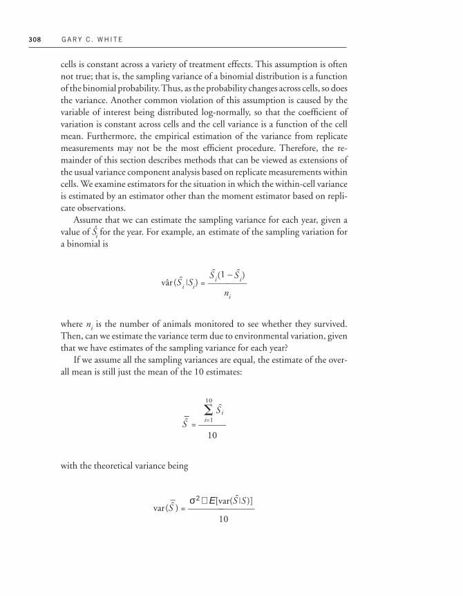
308 GARY C . WH ITE
cells is constant across a variety of treatment effects. This assumption is oftennot true; that is, the sampling variance of a binomial distribution is a functionof the binomial probability. Thus, as the probability changes across cells, so doesthe variance. Another common violation of this assumption is caused by thevariable of interest being distributed log-normally, so that the coefficient ofvariation is constant across cells and the cell variance is a function of the cellmean. Furthermore, the empirical estimation of the variance from replicatemeasurements may not be the most efficient procedure. Therefore, the re-mainder of this section describes methods that can be viewed as extensions ofthe usual variance component analysis based on replicate measurements withincells. We examine estimators for the situation in which the within-cell varianceis estimated by an estimator other than the moment estimator based on repli-cate observations.
Assume that we can estimate the sampling variance for each year, given avalue of Si for the year. For example, an estimate of the sampling variation fora binomial is
vâr(S&i ?Si) = }S&i(1
n
–
i
S&i)}
where ni is the number of animals monitored to see whether they survived.Then, can we estimate the variance term due to environmental variation, giventhat we have estimates of the sampling variance for each year?
If we assume all the sampling variances are equal, the estimate of the over-all mean is still just the mean of the 10 estimates:
S&–
= }10}
with the theoretical variance being
var(S&–) = }
σ2 + Ε[v
1
a
0
r(S&?S )]}
S10
i=1S&i

Population Viability Analysis 309
i.e., the total variance is the sum of the environmental variance plus theexpected sampling variance. This total variance can be estimated as
va&r(S&–) = }
10(10 – 1)}
We can estimate the expected sampling variance as the mean of the sam-pling variances
E&[var(S&?S)] = }10}
so that the estimate of the environmental variance is obtained by solving for σ2
σ&2 = }(10 – 1)
} – }10}
However, sampling variances are usually not all equal, so we have to weightthem to obtain an unbiased estimate of σ2. The general theory says to use aweight, wi ,
wi = }σ2 + var
1
1S&i?Si 2}
so that by replacing var(Si ?Si) with its estimator vâr(Si ?Si), the estimator of theweighted mean is
S10
i=1
1S&i – S&–22
S10
i=1va&r1S&i?Si 2
S10
i=1
1S&i – S&–22
S10
i=1va&r1S&i?Si 2

310 GARY C . WH ITE
S&–
= }}
with theoretical variance (i.e., sum of the theoretical variances for each of theestimates)
var(S&–) = }
1}
and empirical variance estimator
va&r(S&–) =
When the wi are the true (but unknown) weights, we have
}1} = }}
giving the following
1 = }10 – 1}
S10
i=1wi S&i
S10
i=1wi
S10
i=1wi
S10
i=1wi
(S10
i=1wi)(10 – 1)
(S10
i=1wi)(10 – 1)
S10
i=1wi
1S&i – S&–22
S10
i=1wi
1S&i – S&–22
S10
i=1wi
1S&i – S&–22

Population Viability Analysis 311
Therefore, all we have to do is manipulate this equation with a value of σ2 toobtain an estimator of σ2.
To obtain a confidence interval on the estimator of σ2, we can substitutethe appropriate chi-square values in this relationship. To find the upper confi-dence interval value, σ&2
U solve the equation
}10 – 1} =
and for the lower confidence interval value, σ&2L solve the equation
}10
–
1} = }
χ
1
2
0
10
–
–1,
1
αU
As an example, consider the following fawn survival data from overwintersurvival of mule deer fawns at the Little Hills Wildlife Area, west of Meeker,Colorado, USA.
Estimated EstimatedYear Collared Lived Survival Variance
1981 46 15 0.3260870 0.00477731982 114 38 0.3333333 0.00194931983 118 5 0.0423729 0.00034391984 106 19 0.1792453 0.00138791985 155 59 0.3806452 0.00152101986 161 61 0.3788820 0.00146171987 116 15 0.1293103 0.0009706
The survival rates are the number of collared animals that lived divided by the total number of collared animals. For example, S1981 = 15/46 = 0.326087for 1981. The sampling variance associated with this estimate is computed as
S10
i=1wi
1S&i – S&–22
S10
i=1wi
1S&i – S&–22
10 – 1
10 – 1 10 – 1
χ210–1, αL

312 GARY C . WH ITE
var(S&1981) = }S&1981 (1
46
– S&1981)}
which equals 0.0047773. A spreadsheet program (VARCOMP.WB1) com-putes the estimate of temporal process variation for 1981–87, σ2, as 0.0170632(σ = 0.1306262), with a 95 percent confidence interval of (0.0064669,0.0869938) for σ2, and (0.0804167, 0.2949472) for σ. These confidenceintervals represent the uncertainty of the estimate of temporal variation, that is,the sampling variation of the estimate of temporal variation.
The procedure demonstrated here is applicable to estimation of othersources of variation (e.g., spatial variation) and to variables other than survivalrates, such as per capita reproduction. The method is more general than theusual analysis of variance procedures because each observation is not assumedto have the same variance, in contrast to analysis of variance, in which each cellis assumed to have the same within-cell variance.
j Indirect Estimation of Variance Components
Individual heterogeneity occurs in both reproduction and survival. Estimationof individual variation in reproduction is an easier problem than estimation ofindividual variation in survival because some animals reproduce more thanonce, whereas they only die once. Bartmann et al. (1992) demonstrated thatoverwinter survival of mule deer fawns is related to their mass at the start of thewinter. Thus one approach to modeling individual heterogeneity is to find acorrelate of survival that can be measured and develop statistical models of thedistribution of this correlate. Then, the distribution of the correlate can be sam-pled to obtain an estimate of survival for the individual. Lomnicki (1988) alsosuggests mass as an easily measured variable that relates to an animal’s fitness.
To demonstrate this method, I use a simplification of the logistic regressionmodel of Bartmann et al. (1992):
log1}1S
– S}2 = β0 + β1 mass
where survival (S) is predicted as a function of weight. Weight of fawns at thestart of winter was approximately normally distributed, with mean 32 kg and

Population Viability Analysis 313
standard deviation 4.2. To simulate individual heterogeneity in overwinterfawn survival, values can be drawn from this normal distribution to generatesurvival estimates.
This model can be expanded to incorporate temporal variation (year ef-fects), sex effects, and area effects, as described for mule deer fawns by Bartmannet al. (1992). An example of modeling temporal variation in greater flamingos(Phoenicopterus ruber roseus) as a function of winter severity is provided byCézilly et al. (1996). The approach suggested here of modeling winter severityas a random variable and estimating survival as a function of this random vari-able is an alternative to the variance estimation procedures of the previous sec-tion. Both provide a mechanism for injecting variation into a population via-bility model. The main advantage of using weather data to drive the temporalvariation of the model is that considerably more weather data are available thanare biological data on survival or reproductive rates.
The major drawback of the indirect estimation approach proposed in thissection is that sampling variation of the functional relationship is ignored inthe simulation procedure. That is, the logistic regression model includes sam-pling variation because its parameters are estimated from observed data. Theparameter estimates of the logistic regression model include some unknownestimation error. Their direct use results in potentially biased estimates of per-sistence, depending on how much sampling error is present. Therefore, a“good” model relating the covariate to the biological process is needed.
j Bootstrap Approach
Stacey and Taper (1992) used a bootstrap procedure to incorporate temporalvariation into a model of acorn woodpecker (Melanerpes formicivorus) popula-tion viability. They used estimates of adult and juvenile survival and reproduc-tive rates resulting from a 10-year field study to estimate population persis-tence. To incorporate the temporal variation from the 10 years of estimates,they randomly selected with replacement one estimate from the observed val-ues to provide an estimate in the model for a year.
This procedure is known in the statistical literature as a bootstrap samplingprocedure. The technique is appealing because of its simplicity. However, forestimating population viability, a considerable problem is inherent in the pro-cedure. That is, the estimates used for bootstrapping contain sampling varia-tion and demographic variation, as well as the environmental variation thatthe modeler is attempting to incorporate. To illustrate how demographic vari-

314 GARY C . WH ITE
ation is included in the estimates, consider an example population of 10 ani-mals with a constant survival rate of 0.55. Thus, the actual temporal variationis zero, yet a sequence of estimates of survival from this population suggestsconsiderable variation. That is, the estimates of survival would have a varianceof 0.55(1 – 0.55)/10 = 0.02475 if all 10 animals had a survival probability of0.55. Furthermore, the only observed values of survival would be 0, 0.1, . . . ,1.0. However, if the size of the population were increased to 100, you wouldfind that the variance of the sequence of estimates becomes 0.002475, a con-siderable decrease. Thus randomly sampling the estimates from a populationof size 10 results in considerably more variation than from a population of100. As a result, the demographic variation from the sampled population isincorporated into the persistence model if the bootstrap approach is used.
A similar example can be used to demonstrate that sampling variation isalso inherent in bootstrapping from a sample of observed estimates. Suppose asample of 10 radiocollared animals is used to estimate survival for a populationof 100,000 animals (i.e., the finite sample correction term can be ignored).The sampling variation of the estimates would be S(1 – S)/10, where S is thetrue survival rate for the population assuming all animals had the same survivalrate. Now if a sample of 100 radiocollared animals is taken, the sampling vari-ation reduces to S(1 – S)/100. Thus randomly sampling estimates with a boot-strap procedure incorporates the sampling variation of the estimates into thepersistence model. As a result of the increased variation, persistence values willbe underestimated.
Therefore, I suggest not using the bootstrap approach demonstrated byStacey and Taper (1992) if unbiased estimates of persistence are required. Per-sistence estimates developed with this procedure will generally be too low; thatis, you will conclude that the population is more likely to go extinct than itreally will. However, methods such as shrinkage estimation of variances (K. P.Burnham, personal communication 1997) may prove useful in removing sam-pling variance from the estimates and make the bootstrap procedure moreapplicable to estimating population persistence.
j Basic Population Model and Density Dependence
Leslie matrix models (Leslie 1945, 1948; Usher 1966; Lefkovitch 1965;Caswell 1989; Manly 1990) are commonly used as the modeling frameworkfor population viability models. Density dependence must be incorporatedinto the model; that is, basic parameters must be a function of population size.

Population Viability Analysis 315
Thus the resulting model is not a true Leslie matrix. Each iteration of the cal-culation also requires a temporal variance component, and making the param-eters of the Leslie matrix into random variables (Burgman et al. 1993) is thestandard approach but eradicates the analytical results that normally are bene-fits of Leslie’s creative work. If multiple patches are modeled, each patchrequires a spatial variance component. Demographic variation can be builtinto the model. Still, the resulting model doesn’t resemble the elegant matrixmodel that Leslie originally developed.
However, use of the Leslie matrix framework ignores individual hetero-geneity, and thus is likely to underestimate persistence. Incorporation of indi-vidual heterogeneity requires an individual-based model (DeAngelis and Gross1992) and thus is conceptually different from the basic Leslie matrix approach.Individual-based models can be spatially explicit (Conroy et al. 1995; Dun-ning et al. 1995; Holt et al. 1995; Turner et al. 1995), providing another ap-proach to incorporating spatial stochasticity into the model.
As suggested by Boyce (1992), Stacey and Taper (1992), and Burgman etal. (1993), density dependence is an important part of estimating a popula-tion’s persistence. Lande (1993) demonstrates that the importance of environ-mental stochasticity and random catastrophes depends on the density-depen-dence mechanism operating in the population, based on the value of Kcarrying capacity. However, how density dependence is incorporated into themodel greatly affects the estimates of persistence (Pascual et al. 1997). In per-sistence models, as a population declines, compensation for small populationsize takes the form of increased birth rates and decreased death rates (densitydependence) and so is a significant factor in increasing population persistence.
Consider the model
Nt +1 = Nt[1 + R(t)]
Stacey and Taper (1992) tested two forms of density dependence with theirdata; the logistic form
R(t) = R011 – }N
K
(t)}2
and the θ-logistic form

316 GARY C . WH ITE
R(t) = R031 – 1}N
K
(t)}2θ4
Expressed as a difference equation, the θ-logistic model would be
Nt +1 = Nt 51 + R031 – 1}N
K
(t)}2θ46
For θ = 1, the two models are identical. Although Stacey and Taper’s data pre-cluded a significant test between these models, their data did show significantcorrelations between adult survival and population size, suggesting that den-sity dependence was operating in the population.
The distinction between the two models can be very important. In the first,the rate of change of the birth and death rates with population size is linear(i.e., the classic logistic population growth model). In the second, the changecan be very nonlinear. As a result, the θ-logistic model can cause populationsto be very persistent, or very extinction prone, depending on the shape of thefunction. In figure 9.7, the curve for per capita recruitment with θ = 10 resultsin a population with much greater persistence than the curve with θ = 0.1because as the population size becomes small, the θ = 10 population is at peakreproduction for populations below 60, whereas peak reproduction is reachedonly at a population size of zero for the θ = 0.1 population.
Burgman et al. (1993) and May and Oster (1976) summarize other func-tional relationships to incorporate density dependence. Possibilities, expressedas a difference equations, include those by Hassell (1975), Hassell et al.(1976), and May (1976):
Nt +1 = }(1 +
λ
a
N
Nt
t )b
}
by Moran (1950) and Ricker (1954, 1975:282):
Nt +1 = Nt exp3r11 – }N
Kt}24

Population Viability Analysis 317
by Pennycuick et al. (1968), Usher (1972), and Beddington (1974), takenfrom May and Oster (1976):
Nt +1 =
by Beverton and Holt (1957) and Ricker (1975):
Nt +1 = }ρ + (
1
k /Nt )}
and by Maynard-Smith and Slatkin (1973):
λNt}}}1 + exp[– A(1 – Nt /B)]
Figure 9.7 Three examples of possible relationships of recruitment per individual to populationsize (Nt). Typical sigmoid population growth demonstrated by the logistic curve results for θ = 1. Asteeper curve initially results for θ = 0.1, whereas a flatter curve initially results for θ = 10.

318 GARY C . WH ITE
Nt +1 =
Each of these models results in a different relationship between per capitarecruitment and population size. Furthermore, these simple models can beapplied to various segments of the life cycle, such as fecundity rates, neonatalsurvival, and adult survival, to achieve more realistic biological models. Butthe use of different models means that density dependence is implemented dif-ferently at a particular population level and population viability is affected. Forexample, Mills et al. (1996) reported widely differing estimates of populationviability of grizzly bear (Ursus arctos horribilis) depending on which of fourcomputer programs were used to compute the estimate. Probably part of thediscrepancy is in how density dependence was implemented in each of the pro-grams, but different functions probably were used and these relationshipsprobably were applied to differing segments of the life cycle. Unfortunately,distinguishing between these various models of density dependence with datais not practical because of the stochasticity (noise) in observed population lev-els, as Pascual et al. (1997) demonstrated by fitting a collection of models toSerengeti wildebeest (Connochaetes taurinus) data.
Fowler (1981, 1994) argues that both theory and empirical informationsupport the conclusion that most density-dependent change occurs at highpopulation levels (close to the carrying capacity) for species with life historystrategies typical of large mammals, such as deer (θ > 1). The reverse is true forspecies with life history strategies typical of insects and some fishes, with θ < 1).
Note that explicit estimates of carrying capacity (K ) and its variance are notneeded to incorporate density dependence into a population model, althoughsuch an approach is possible. If the functional relationships between birth anddeath rates and population density are available, the carrying capacity is deter-mined by these relationships. Furthermore, if these relationships incorporatetemporal and spatial variation, then the resulting model will have temporaland spatial variation in its carrying capacity, and thus stochastic densitydependence.
Another example of how density dependence can operate in small popula-tions is provided by the Allee effect (Allee 1931): The per capita birth ratedeclines at low densities (figure 9.8) because, for example, of the increased dif-ficulty of finding a mate (Yodzis 1989). This is known as Allee-type behavior(of the per capita birth rate), and its effect on the per capita population growthrate, R(t), is called an Allee effect. In theory, a low-density equilibrium would
R0Nt}}1 + (R0 – 1)1}
N
kt}2
c

Population Viability Analysis 319
be sustained in a deterministic equilibrium, where the birth rate equals thedeath rate. However, given stochasticity, the population could be driven belowthe low density equilibrium, and thus slide into extinction.
A second example of incorporating density dependence into a populationviability analysis is provided by Armbruster and Lande (1993). They used esti-mates of life history parameters of elephant (Loxodonta africana) populationsin a fluctuating environment from studies at Tsavo National Park, Kenya, todevelop an age-structured, density-dependent model. Density regulation wasimplemented by changes in the age of first reproduction and calving interval.They modeled environmental stochasticity with drought events affecting sex-and age-specific survival.
j Incorporation of Parameter Uncertainty into Persistence Estimates
In a previous section, I demonstrated how to remove the sampling variationfrom estimates of process variation. Unbiased estimates of process variancessuch as temporal and spatial variation can be achieved. In this section, I exam-
Figure 9.8 Example of how an Allee effect is created by a declining birth rate at low densities. Twoequilibrium points exist, where the birth rate equals the death rate. The lower equilibrium may bestable in a deterministic system but could easily lead to extinction in a stochastic system.

320 GARY C . WH ITE
ine how to incorporate uncertainty of the parameter estimates into the esti-mates of persistence and, in the process, provide an unbiased estimate of per-sistence given the population model.
Any model developed to estimate population persistence has several tomany parameters that must be estimated from available data. Each of theseestimates has an associated estimate of its precision in the form of a variance,assuming that statistically rigorous methods were used to estimate the param-eter from data. In addition, because some of the parameters may have beenestimated from the same set(s) of data, some parameters in the model mayhave a nonzero covariance. Thus, the vector of parameter estimates θ& used inthe model to estimate persistence has the variance–covariance matrix [vâr(θ&)]to measure uncertainty.
Typically, statisticians use the delta method (Seber 1982) to estimate thevariance of a function of parameters from a set of parameter estimates andtheir variance–covariance matrix. In the context of persistence, the samplingvariance of the estimate of persistence (p ) would be estimated from the sam-pling variances of the parameters in the model as
va&r(p&) = }δf
δ
(
θ
θ&)T
} va&r(θ&) }δf
δ
(
θ
θ&)}
where p&= f (θ&). That is, the function f represents the model used to estimatepersistence. However, for realistically complex persistence models, the analyt-ical calculation of partial derivatives needed in this formula is probably not fea-sible.
The lack of explicit analytical partial derivatives suggests that numericalmethods be used. The most feasible, albeit numerically intensive, appears to bethe parametric bootstrap approach (Efron and Tibshirani 1993; Urban Hjorth1994). With a parametric bootstrap, a realization of the parameter estimates isgenerated based on their point estimates and sampling variance–covariancematrix using Monte Carlo methods. A multivariate normal distribution prob-ably is used as the parametric distribution describing the set of parameter esti-mates, although other distributions or combinations of distributions may bemore realistic biologically. Using this set of simulated values in the persistencemodel, persistence is estimated. This step requires a large number of simula-tions to properly estimate persistence with little uncertainty; typically 10,000simulations are conducted. Then, a new set of parameter values is generated

Population Viability Analysis 321
and persistence again estimated. This process is repeated for many sets ofparameter estimates (at least 100, but more likely 1,000) to obtain a set of esti-mates of persistence. The variation of the resulting estimates of persistence isthen a measure of uncertainty attributable to the variation of the parameterestimates as measured by their variance–covariance matrix. The process is dia-grammed as
PARAMETRIC BOOTSTRAP LOOP (1,000 iterations):Select realization of parameter estimates
MONTE CARLO LOOP (10,000 iterations):Tabulate percentage of model runs resulting in persistence
END MONTE CARLO LOOPEND PARAMETRIC BOOTSTRAP LOOP
However, even more critical to our viability analysis is the fact that themean of this set of 1,000 estimates of persistence is probably less than the esti-mate we obtained using our original point estimates of model parameters.More formally, the expected value of estimated persistence
[E(p )]
is less than the value of persistence predicted by our model using the point esti-mates of its parameters,
E(p )< f [E(θ)]
an example of Jensen’s inequality. This difference is caused by large probabili-ties of early extinction for certain parameter sets that are likely, given theirsampling variation (Ludwig 1996a). Therefore, to estimate persistence, themean of the bootstrap estimates of persistence should be used, not the estimateof persistence obtained by plugging our parameter estimates directly into ourpopulation model.
Confidence intervals on persistence could be constructed using the usual±2 SE procedure based on the set of 1,000 estimates. This confidence intervalrepresents the variation attributable to the uncertainty of the parameter esti-
322 GARY C . WH ITE
mates used in the model. Uncertainty about the model is not included in thisconfidence interval because the model is assumed to be known. However, abetter confidence interval will probably be achieved by sorting the 1,000 val-ues into ascending order and using the 25th and 975th values as a 95 percentconfidence interval. This procedure accounts for the likely asymmetric distri-bution of the estimates of persistence.
j Discussion
The real problem with PVA is not the model, but obtaining the data to drivethe model (Ruggiero et al. 1994). Much of the published work on PVA ignoresthis essential point (Thomas 1990). For example, Mangel and Tier (1994:608–611) simplify the process to the point that they miss major issues con-cerning data reliability and quality of the product (estimates of persistence).Their four “facts” are as follows:
• “A population can grow, on average, exponentially and without bound andstill not persist.” This is because of catastrophes that will bring even a thrivingpopulation to zero.
• “There is a simple and direct method for the computation of persistencetimes that virtually all biologists can use.” They suggest a simple model withone age class and a population ceiling that the population cannot exceed, butthe ceiling does not cause density dependence effects of growth parameters. Asa result, their approach to estimating persistence is likely to underestimate per-sistence if the ceiling is set too low because the population can never grow awayfrom the absorbing state of extinction.
• “The shoulder of the MacArthur–Wilson model occurs with other modelsas well, but disappears when catastrophes are included.” They suggest a slow,steady rise in persistence times as the population ceiling is increased.
• “Extinction times are approximately exponentially distributed and thismeans that extinctions are likely.” Thus, they conclude the most likely value ofa population is zero, or the mode of an exponential distribution. I believe thisresult is obtained because of the simplistic assumptions they have used. Realis-tic models that incorporate the sources of variation described in this chapterdo not result in such simplistic results.

Population Viability Analysis 323
Another misguided example is Tomiuk and Loeschcke (1994). Theirmathematics cover up the real problem of obtaining realistic estimates of theparameter values to use in the models. Their model emphasizes demographicvariation and ignores the bigger issues of temporal variation and individualheterogeneity.
A common problem with PVA is that the sampling variation of the param-eter estimates is ignored (e.g., Stacey and Taper 1993; Dennis et al. 1991). Inboth cases, estimates of persistence are too pessimistic because the samplingvariation of the population parameters is included in the population model asif it were temporal variation. Furthermore, individual heterogeneity was leftout of the model, further biasing the estimates of persistence too low.
“Most PVAs have ignored fundamentals of ecology such as habitat, focus-ing instead on genetics or stochastic demography” (Boyce 1992:491). Forsmall populations (less than 50) of endangered species, such a strategy may bejustified, particularly for short-term predictions. But incorporating onlydemographic variation results in overestimates of persistence because temporalvariation has been ignored. On the other hand, the remaining survivors of anendangered species may be the individuals with high survival and reproductiverates, so the lack of individual heterogeneity may underestimate persistence.
The studies just mentioned should not lead the reader to believe that use-ful attempts to estimate persistence do not exist. Schneider and Yodzis (1994)developed a model of marten (Martes americana) population dynamics thatincorporated the behavior and physiology of individual martens, spatialdynamics, and demographic and environmental stochasticity. Undoubtedlysome readers would quibble with some of the assumptions and data used tobuild the model, but I contend that a realistic model with some of the inputsguessed (and clearly stated to be such) is a much more reasonable approachthan a simplistic model that ignores important processes affecting persistence.Furthermore, such realistic models identify data needs that can be addressedwith time, even though the actual estimate of persistence is of questionablevalue. The alternative of using simplistic and naive models leads to invalid esti-mates and little progress in improving the situation, with a rapid loss of credi-bility by the field of conservation biology.
Murphy et al. (1990) proposed two different types of PVA. For organismswith low population densities that are restricted to small geographic ranges(typical vertebrate endangered species), genetic and demographic factorsshould be stressed. For smaller organisms such as most endangered inverte-brates, environmental uncertainty and catastrophic factors should be stressedbecause these organisms are generally restricted to a few small habitat patches,

324 GARY C . WH ITE
but are capable of reaching large population sizes within these patches. Nun-ney and Campbell (1993) noted that demographic models and genetic mod-els both have resulted in similar estimates of minimum viable population size,but that the ideal spatial arrangement of reserves remains an issue.
Lande (1995) suggests that genetic mutations may affect fitness, so ignor-ing genetic effects results in underestimates of viability. Mutation can affectthe persistence of small populations by causing inbreeding depression, bymaintaining potentially adaptive genetic variation in quantitative characters,and through the erosion of fitness by accumulation of mildly detrimentalmutations. Populations of 5,000 or more are required to maintain evolution-ary viability. Theoretical results suggest that the risk of extinction caused bythe fixation of mildly detrimental mutations may be comparable in impor-tance to environmental stochasticity and could substantially decrease the long-term viability of populations with effective sizes as large as a few thousand(Lande 1995). If these results are correct, determining minimum viable popu-lation numbers for most endangered species is an exercise in futility becausealmost all of these populations are already below 5,000.
Conservation biologists would like to have rules to evaluate persistence(Boyce 1992), such as the magical Franklin–Soulé number of 500 (Franklin1980; Soulé 1980) that is the effective population size (Ne) to maintain geneticvariability in quantitative characters. Unfortunately, these rules lack the realismto be useful. The Franklin–Soulé number was derived from simple geneticmodels and hence lacks the essential features of a PVA model discussed here.Attempts with simplistic models such as Mangel and Tier (1994) and Tomiukand Loeschcke (1994) also do not provide defensible results because of the lack of attention to the biology of the species and the stochastic environ-ment in which the population exists. Until conservation biologists do goodexperimental studies to evaluate population persistence empirically, I questionthe usefulness of the rules and simplistic models suggested in some of theliterature.
PVA can be viewed as a heuristic tool to explore the dynamics of an endan-gered population but not as a predictive tool. PVA could be used to identifyvariables to which the population may be sensitive and to investigate the rela-tive benefits of alternative kinds of management. Some readers will argue thatin this context, the absolute reliability of the model estimates of extinctionprobability, or time to extinction, matters much less than the extent to whichrisk is affected by different demographic and environmental variables. I dis-agree because conclusions from PVA so strongly depend on which sources ofvariation are included in the model and their relative magnitudes. For exam-ple, the importance of demographic variation is stressed in PVA because it

Population Viability Analysis 325
happens to be the simplest source of variation to model, generally requiringonly the assumption of binomial variation. Temporal variation has receivedless emphasis because it is a more difficult to obtain estimates of the temporalvariance of population parameters. Individual heterogeneity has received noattention because this source of variation is by far the most difficult source toquantify, particularly for survival rates. The only way to draw valid inferencesabout the importance of various sources of stochasticity affecting a populationis to have reasonably good estimates of these parameters. Simplistic PVA mod-els based on few or no data lead to simplistic and unreliable answers. Withoutdata, why would you expect anything else?
Until rigorous experimental work can be conducted, conservation biolo-gists should borrow information from game species, where long-term studieshave been done that will provide estimates of temporal and spatial variationand individual heterogeneity. Rules that predict temporal variation in survivalas a function of weather, or individual variation in survival as a function ofbody characteristics, provide alternative sources of data. For at least some gamespecies, data exist to develop such rules. Furthermore, these kinds of dataprobably will never be available for many endangered species; the opportunityto collect such data was lost with the decline of the population to current(threatened) levels. Thus I suggest the use of surrogate species to help meet thedata needs of realistic models of persistence. Taxonomically related species mayprovide information, although species in the same ecological guild may alsoprovide information on temporal and spatial variation. Note the distinctionbetween using estimates of the temporal and spatial variation and individualheterogeneity from a related species and using estimates of survival andrecruitment from a surrogate species. Estimates of survival and recruitmentfrom a stable or increasing population would obviously be inappropriate for aspecies with a declining population.
j Conclusion
In summary, most estimates of population viability are nearly useless becauseone or more of the following mistakes or omissions are made in developing amodel to estimate persistence. By listing omissions, this list suggests the essen-tial ingredients to develop a useful PVA.
• Few or no data are available to estimate basic parameters in the populationmodel, with almost all the parameter estimates just guesses. The resulting esti-mate of persistence is therefore strictly a guess.

326 GARY C . WH ITE
Lesson: To do a valid PVA, you must have data to build a realistic popula-tion model.
• The model ignores spatial variation, which increases population viability.As suggested by Stacey and Taper (1992), immigration can occasionally rescuea population from extinction.
Lesson: If the population is widely distributed geographically, incorporatespatial variation.
• The model uses estimates of temporal variation that are at best poorguesses. This statement assumes that the modeler understood the differencebetween process variation and sampling variation. Often, sampling variation isassumed to substitute for process variation; as a result, the estimates of persis-tence are too pessimistic. Sampling variation has nothing to do with popula-tion persistence. Estimates of population parameters must not be treated as ifthey are the true parameter value.
Lesson: Obtain reliable estimates of temporal variation and don’t confusesampling variation and temporal variation.
• The model uses demographic variation as a substitute for temporal varia-tion in the process and ignores true temporal variation.
Lesson: Incorporate both demographic and temporal variation into thePVA.
• The model ignores life-long individual heterogeneity that increases popu-lation viability and assumes that all individuals endure the same identical sur-vival and reproduction parameters. Such a naive assumption results in popula-tion viability being underestimated.
Lesson: Individual heterogeneity must be incorporated into a PVA model ifyou don’t want to underestimate viability.
• The model assumes that current conditions are not changing; that is, thestochastic processes included in the model are assumed constant for the indef-inite future. Loss of habitat and other environmental changes that affect thesestochastic processes are ignored. Thus, as discussed by Caswell (1989), themodel probably is not useful in forecasting (i.e., predicting what will happen)but is useful in projecting (i.e., predicting what will happen if conditions donot change).

Population Viability Analysis 327
Lesson: Recognize that your model does not predict the future; it only proj-ects what might happen if the system doesn’t change (which is unlikely).
Before you use the estimates of persistence from any population viabilityanalysis, compare the approach used to obtain the estimate with the necessarycomponents discussed here. If you discover omissions and errors in the ap-proach used to obtain the estimate, recognize the worth (or lack thereof ) of theestimate of persistence. Although the estimates of persistence obtained from aPVA may have little value, the process of formulating a model and identifyingmissing information (i.e., parameters that are poorly estimated) may still havevalue in developing measures to conserve the species in question.
Literature Cited
Allee, W. C. 1931. Animal aggregations. Chicago: University of Chicago Press.Armbruster, P. and R. Lande. 1993. A population viability analysis for African elephant
(Loxodonta africana): How big should reserves be? Conservation Biology 7: 602–610.Bartmann, R. M., G. C. White, and L. H. Carpenter. 1992. Compensatory mortality in a
Colorado mule deer population. Wildlife Monographs 121: 1–39.Beddington, J. R. 1974. Age distribution and the stability of simple discrete time popula-
tions models. Journal of Theoretical Biology 47: 65–74.Beissinger, S. R. 1995. Modeling extinction in periodic environments: Everglades water lev-
els and Snail Kite population viability. Ecological Applications 5: 618–631.Bennington, C. C. and W. V. Thayne. 1994. Use and misuse of mixed model analysis of
variance in ecological studies. Ecology 75: 717–722.Berger, J. 1990. Persistence of different-sized populations: An empirical assessment of rapid
extinctions in bighorn sheep. Conservation Biology 4: 91–98.Beverton, R. J. H. and S. J. Holt. 1957. On the dynamics of exploited fish populations.
Great Britain Ministry of Agriculture, Fisheries and Food, Fishery Investigations (Series 2)19: 5–533.
Boyce, M. S. 1992. Population viability analysis. Annual Review of Ecology and Systematics23: 481–506.
Burgman, M. A., S. Ferson, and H. R. Akçakaya. 1993. Risk assessment in conservation biol-ogy. London: Chapman & Hall.
Burnham, K. P., D. R. Anderson, and G. C. White. 1996. Meta-analysis of vital rates of thenorthern spotted owl. Studies in Avian Biology 17: 92–101.
Burnham, K. P., D. R. Anderson, G. C. White, C. Brownie, and K. H. Pollock. 1987.Design and analysis experiments for fish survival experiments based on capture–recap-ture. American Fisheries Society Monograph 5: 260–278.
Caswell, H. 1989. Matrix population models. Sunderland, Mass.: Sinauer.Caughley, G. 1994. Directions in conservation biology. Journal of Animal Ecology 63:
215–244.

328 GARY C . WH ITE
Cézilly, F., A. Viallefont, V. Boy, and A. R. Johnson. 1996. Annual variation in survival andbreeding probability in greater flamingos. Ecology 77: 1143–1150.
Clark, T. W., P. C. Paquet, and A. P. Curlee. 1996. Special section: Large carnivore conser-vation in the Rocky Mountains of the United States and Canada. Conservation Biology10: 936–936.
Clutton-Brock, T. H., F. E. Guinness, and S. D. Albon. 1982. Red deer: Behavior and ecol-ogy of two sexes. Chicago: University of Chicago Press.
Conroy, M. J., Y. Cohen, F. C. James, Y. G. Matsinos, and B. A. Maurer. 1995. Parameterestimation, reliability, and model improvement for spatially explicit models of animalpopulations. Ecological Applications 5: 17–19.
DeAngelis, D. L. and L. J. Gross, eds. 1992. Individual-based models and approaches in ecol-ogy: Populations, communities, and ecosystems. New York: Chapman & Hall.
Dennis, B., P. L. Munholland, and J. M. Scott. 1991. Estimation of growth and extinctionparameters for endangered species. Ecological Monographs 6: 115–143.
Diamond, J. and S. Pimm. 1993. Survival times of bird populations: A reply. American Nat-uralist 142: 1030–1035.
Dunning, J. B. Jr., D. J. Stewart, B. J. Danielson, B. R. Noon, T. Root, R. H. Lamberson,and E. E. Stevens. 1995. Spatially explicit population models: Current forms and futureuses. Ecological Applications 5: 3–11.
Efron, B. and R. J. Tibshirani. 1993. An introduction to the bootstrap. New York: Chapman& Hall.
Foley, P. 1994. Predicting extinction times from environmental stochasticity and carryingcapacity. Conservation Biology 8: 124–136.
Fowler, C. W. 1981. Density dependence as related to life history strategy. Ecology 62:602–610.
Fowler, C. W. 1994. Further consideration of nonlinearity in density dependence amonglarge mammals. Report of the International Whaling Commission 44: 385–391.
Franklin, I. R. 1980. Evolutionary changes in small populations. In M. E. Soulé and B. A.Wilcox, eds., Conservation biology: An evolutionary–ecological perspective, 135–149.Sunderland, Mass.: Sinauer.
Ginzburg, L. R., L. B. Slobodkin, K. Johnson, and A. G. Bindman. 1982. Quasiextinctionprobabilities as a measure of impact on population growth. Risk Analysis 2: 171–181.
Haila, Y. and I. K. Hanski. 1993. Birds breeding on small British islands and extinctionrisks. American Naturalist 142: 1025–1029.
Hanski, I. 1996. Metapopulation ecology. In O. E. Rhodes, Jr., R. K. Chesser, and M. H.Smith, eds., Population dynamics in ecological space and time, 13–43. Chicago: Univer-sity of Chicago Press.
Hanski, I., A. Moilanen, and M. Gyllenberg. 1996. Minimum viable metapopulation size.American Naturalist 147: 527–541.
Hassell, M. P. 1975. Density-dependence in single-species populations. Journal of AnimalEcology 44: 283–295.
Hassell, M. P., J. H. Lawton, and R. M. May. 1976. Patterns of dynamical behaviour in sin-gle-species populations. Journal of Animal Ecology 45: 471–486.

Hess, G. R. 1993. Conservation corridors and contagious disease: a cautionary note. Con-servation Biology 8: 256–262.
Holt, R. D., S. W. Pacala, T. W. Smith, and J. Liu. 1995. Linking contemporary vegetationmodels with spatially explicit animal population models. Ecological Applications 5:20–27.
Hunter, M. L., Jr. 1996. Fundamentals of conservation biology. Cambridge, Mass.: Blackwell.Joopouborg, N. and J. M. Van Groenendael. 1996. Demography, genetics, or statistics:
Comments on a paper by Heschel and Paige. Conservation Biology 10: 1290–1291.Keller, L. F., P. Arcese, J. N. M. Smith, W. M. Hochachka, and S. C. Stearns. 1994. Selec-
tion against inbred song sparrows during a natural population bottleneck. Nature 372:356–357.
Koenig, W. D., R. L. Mumme, W. J. Carmen, and M. T. Stanback. 1994. Acorn produc-tion by oaks in central California: Variation within and among years. Ecology 75:99–109.
Krausman, P. R., R. C. Etchberger, and R. M. Lee. 1993. Persistence of mountain sheep.Conservation Biology 7: 219.
Lande, R. 1988. Genetics and demography in biological conservation. Science 241:1455–1460.
Lande, R. 1993. Risks of population extinction from demographic and environmental sto-chasticity and random catastrophes. American Naturalist 142: 911–927.
Lande, R. 1995. Mutation and conservation. Conservation Biology 9: 782–791.Lefkovitch, L. P. 1965. The study of population growth in organisms grouped by stages.
Biometrics 21: 1–18.Leslie, P. H. 1945. On the use of matrices in certain population mathematics. Biometrika
33: 183–212.Leslie, P. H. 1948. Some further notes on the use of matrices in population mathematics.
Biometrika 35: 213–245.Lomnicki, A. 1988. Population ecology of individuals. Princeton, N.J.: Princeton University
Press.Ludwig, D. 1996a. Uncertainty and the assessment of extinction probabilities. Ecological
Applications 6: 1067–1076.Ludwig, D. 1996b. The distribution of population survival times. American Naturalist 147:
506–526.Mace, G. M. and R. Lande. 1991. Assessing extinction threats: Toward a reevaluation of
IUCN threatened species categories. Conservation Biology 5: 148–157.Mangel, M. and C. Tier. 1994. Four facts every conservation biologist should know about
persistence. Ecology 75: 607–614.Manly, B. F. J. 1990. Stage-structured population sampling, analysis and simulation. London:
Chapman & Hall.May, R. M. 1976. Models for single populations. In R. M. May, ed., Theoretical ecology:
Principles and applications, 4–25. Oxford, U.K.: Blackwell Scientific.May, R. M. and G. F. Oster. 1976. Bifurcations and dynamic complexity in simple ecolog-
ical models. American Naturalist 110: 573–599.
Population Viability Analysis 329

330 GARY C . WH ITE
Maynard-Smith, J. and M. Slatkin. 1973. The stability of predator–prey systems. Ecology54: 384–391.
Meffe, G. K. and C. R. Carroll. 1994. Principles of conservation biology. Sunderland, Mass.:Sinauer.
Mills, L. S., S. G. Hayes, C. Baldwin, M. J. Wisdom, J. Citta, D. J. Mattson, and K. Mur-phy. 1996. Factors leading to different viability predictions for a grizzly bear data set.Conservation Biology 10: 863–873.
Moran, P. A. P. 1950. Some remarks on animal population dynamics. Biometrics 6:250–258.
Murphy, D. D., K. E. Freas, and S. B. Weiss. 1990. An environment-metapopulationapproach to population viability analysis for a threatened invertebrate. ConservationBiology 4: 41–51.
Nunney, L. and K. A. Campbell. 1993. Assessing minimum viable population size: Demog-raphy meets population genetics. Trends in Ecology and Evolution 8: 234–239.
Pascual, M. A., P. Kareiva, and R. Hilborn. 1997. The influence of model structure on con-clusions about the viability and harvesting of Serengeti wildebeest. Conservation Biology11: 966–976.
Pennycuick, C. J., R. M. Compton, and L. Beckingham. 1968. A computer model for sim-ulating the growth of a population or of two interacting populations. Journal of Theo-retical Biology 18: 316–329.
Pimm, S. L., H. L. Jones, and J. M. Diamond. 1988. On the risk of extinction. AmericanNaturalist 132: 757–785.
Remmert, H., ed. 1994. Minimum animal populations. New York: Springer-Verlag.Ricker, W. E. 1954. Stock and recruitment. Journal of the Fisheries Research Board of Canada
11: 559–623.Ricker, W. E. 1975. Computation and interpretation of biological statistics of fish populations.
Ottawa: Fisheries Research Board of Canada, bulletin 191.Ruggiero, L. F., G. D. Hayward, and J. R. Squires. 1994. Viability analysis in biological
evaluations: Concepts of population viability analysis, biological population, and eco-logical scale. Conservation Biology 8: 364–372.
Schneider, R. R., and P. Yodzis. 1994. Extinction dynamics in the American marten (Martesamericana). Conservation Biology 4: 1058–1068.
Seber, G. A. F. 1982 (2d ed.). Estimation of animal abundance and related parameters. NewYork: Macmillan.
Shaffer, M. L. 1981. Minimum population size for species conservation. BioScience 31:131–134.
Shaffer, M. L. 1987. Minimum viable populations: Coping with uncertainty. In M. E.Soulé, ed., Viable populations for conservation, 69–86. Cambridge, U.K.: CambridgeUniversity Press.
Silva, M. and J. A. Downing. 1994. Allometric scaling of minimal mammal densities. Con-servation Biology 8: 732–743.
Soulé, M. E. 1980. Thresholds for survival: maintaining fitness and evolutionary potential.

In M. E. Soulé and B. A. Wilcox, eds., Conservation biology: An evolutionary-ecologicalperspective, 151–170. Sunderland, Mass.: Sinauer.
Soulé, M. E. 1987. Viable populations for conservation. New York: Cambridge UniversityPress.
Stacey, P. B. and M. Taper. 1992. Environmental variation and the persistence of small pop-ulations. Ecological Applications 2: 18–29.
Thomas, C. D. 1990. What do real population dynamics tell us about minimum viablepopulation sizes? Conservation Biology 4: 324–327.
Thomas, C. 1994. Extinction, colonization, and metapopulations: Environmental trackingby rare species. Conservation Biology 8: 373–378.
Tomiuk, J. and V. Loeschcke. 1994. On the application of birth–death models in conser-vation biology. Conservation Biology 8: 574–576.
Tracy, C. R. and T. L. George. 1992. On the determinants of extinction. American Natu-ralist 139: 102–122.
Tracy, C. R. and T. L. George. 1993. Extinction probabilities for British island birds: Areply. American Naturalist 142: 1036–1037.
Turner, M. G., G. J. Arthaud, R. T. Engstrom, S. J. Hejl, J. Liu, S. Loeb, and K. McKelvey.1995. Usefulness of spatially explicit population models in land management. Ecologi-cal Applications 5: 12–16.
Urban Hjorth, J. S. 1994. Computer intensive statistical methods. London: Chapman &Hall.
Usher, M. B. 1966. A matrix approach to the management of renewable resources, withspecial reference to selection forests. Journal of Applied Ecology 3: 355–67.
Usher, M. B. 1972. Developments in the Leslie matrix model. In J. N. R. Jeffers, ed., Math-ematical models in ecology, 29–60. Oxford, U.K.: Blackwell.
Yodzis, P. 1989. Introduction to theoretical ecology. New York: Harper & Row.
Population Viability Analysis 331

Chapter 10
Measuring the Dynamics of Mammalian Societies:An Ecologist’s Guide to Ethological MethodsDavid W. Macdonald, Paul D. Stewart, Pavel Stopka, andNobuyuki Yamaguchi
Today, biologists interpret behavior within a context fortified by theories ofcognition, behavioral evolution, and games (Axelrod 1984; Findlay et al.1989; Hemelrijk 1990; Hare 1992; de Waal 1992), and any or all of fourprocesses may lead to cooperation: kin selection, reciprocity and byproductmutualism, and even trait-group selection (reviewed by Dugatkin 1997). Theprocesses that fashion societies are set within an ecological context (Macdon-ald 1983), and a species’ ecology can scarcely be interpreted without under-standing its social life. As the specialties within whole-animal biology diversifyand the once close-knit family of behavioral and ecological disciplines risksdrifting apart, our purpose is to alert ecologists to the ethologist’s tools formeasuring social dynamics.
j Social Dynamics
“If animals live together in groups their genes must get more benefit out of theassociation than they put in” (Dawkins 1989). What methods are available tomeasure the negotiations—the social dynamics—in this profit and lossaccount? We define a social dynamic simply as the change in social interactionor relationship under the influence of extrinsic or intrinsic factors. Our pur-pose here is to show how these changes and the factors influencing them maybe measured and identified. Likely candidates include the forces of ecologicaland demographic change, together with changes in the experiences and char-acters of group members. Ontogenic effects (individuals growing up and

Measuring the Dynamics of Mammalian Societies 333
changing roles) might also affect the long-term social dynamics of a group thatchange the demography and hence the character of the society (Geffen et al.1996). Effects on social dynamics may be erratically stochastic or predictablycircadian, seasonal, annual, or of an even longer periodicity, largely followingenvironmental rhythms. Predictable changes in social structure may also fol-low as a population or group progresses in a social succession toward carryingcapacity after colonization or population crashes. Against this backdrop ofalmost continual flux, the study of social dynamics requires the measurementof changes in behavioral parameters. These measures become the currencywith which to assess predictions designed to test whether the forces of changehave been isolated correctly. The concept of a group’s social dynamic is a vitaland often neglected foil to attempts to characterize a typical social structure.Therefore, the concept of social dynamics lies at the interface of sociobiology,ethology, and behavioral ecology and even includes aspects of complexity the-ory and emergent systems. This alone makes it a topic of dauntingly largescope.
Research on social behavior commonly seeks a conclusion as to whether aparticular type of social interaction maximizes fitness (Krebs and Davies1991). However, to avoid the hazards of naive interpretation, one cannot drawsuch a conclusion without knowing the pattern of other interactions withinwhich the behavior in question is set. Behavioral ecologists may pick individ-uals for which they score an approximation of fitness against a continuum ofstrategies. This approach is more hazardous as the web of social interactions inwhich individuals of a species are enmeshed becomes more complex. Occam’srazor may suggest making the simplest explanation on the basis of what youobserve, but in a social network the system is seldom simple, so it is prudent tomake those observations thoroughly and in a wide context before that razorcan be wielded confidently.
That the social dynamics of a species are both determinants and conse-quences of its ecology may be clear. To a field ecologist seeking to understandany part of this loop, it may be much less obvious how to characterize a socialsystem in replicable, enduring, and quantitative terms as a basis for modernanalysis. Historically, ethology pursued its own agenda—often with captiveprimates—of characterizing societies by observing behavioral interactions anddirectionality of behaviors within groups (Hemelrijk 1990). Classic etholo-gists were careful to record the detail of behavior with a view to allowing com-parisons between studies and between species; although modern comparativemethods have brought elegance to the task of making comparisons, modern

334 MACDONALD , STEWART, STOPKA , AND YAMAGUCHI
fashions have drifted away from assembling the data classic ethologists so care-fully gleaned.
j Context
In a book on ecological methods, the function of this chapter is to provide a mapfor ecologists through the portions of the rapids that ethologists have alreadynegotiated. When we launched into this task, no text existed to bring togetherthe wisdom of a receding era of ethology and the innovations promised by avantgarde methods; as we finished, Lehner’s (1996) comprehensive second editionHandbook of Ethological Methods was published. Lehner’s updated text is set tobecome the benchmark, so for many topics for which this chapter whets thereader’s appetite, that handbook will be the place to find the full meal.
Our treatment has five sections. First we mention three reasons why docu-menting social dynamics is important. Second, we tackle the question of howto describe social dynamics in ways that provide a framework within which tocompare studies; in this, we follow Hinde (1981, 1983) in describing a hierar-chical approach to the study of social dynamics. We show that single behavioralinteractions are the fundamental unit of social structure, and that it is thechanging nature of repeated interactions—relationships—that gives socialstructure its potentially dynamic component. Third, we follow this frameworkto discuss how behavioral parameters can be described, classified, and recordedduring social interactions. In this we explore interactions during grooming anddominance. In the fourth section we explore methods used for gathering dataon social interaction and then, in the fifth section, we use example data to illus-trate analytical techniques for elucidating relationships, and how patterns ofrelationships can be combined to reveal social networks and social structure.Because mammalian societies are ethologically complex and because our ownexperience is largely with mammals, we draw our examples from that class. Fur-thermore, we often use examples from our own work, not because it deservesmention more than any other, but because we know most well the lessonslearned and pitfalls encountered therein; our intention is merely to illustratepoints, not to review them compendiously (that task is more fully accomplishedby Colgan 1978; Hazlett 1977; and Lehner 1996). Throughout, we focus oncommon mistakes in approach, methodological conflicts, and the use of newtechnology to solve problems (and how it creates some new ones). We havedoubtless fallen short of our own prescriptions on many previous occasions,and are aware that many methods outlined here could be improved further.

Measuring the Dynamics of Mammalian Societies 335
j Why Study Social Dynamics?
Social dynamics merit study for three major reasons. First, the changing rela-tionships between individuals are the building blocks from which dynamicsocial structures are assembled. Understanding their emergent properties, suchas dominance hierarchies and social competition, is essential to tackling fun-damental questions about the evolution of sociality (Pollock 1994). Second,because social dynamics are the product of interaction between individuals’ecology and behavior (Rubenstein 1993), they are relevant to predicting andmanaging the consequences of many human interventions for conservation ormanagement. Third, an important motivation for understanding nonhumansocieties is the light this throws on human behavior. Each of these three topicsis vast, but we fleetingly mention them in turn.
EVOLUTION OF SOCIALITY
The diverse relationships of individuals in a social network interact to createcomplex emergent patterns. These patterns, like the vortex that appears in anemptying sink, is not contained in the structure of a single component.Because a society represents a whole with properties different from those of itscomponent parts, the ultimate consequences of social interactions may beremote from an observed action. This is a fact that evolution by natural selec-tion can take in its stride but that we, as primarily linear cause-and-effectthinkers, may find hard to accommodate. It may be clear that a lion killing azebra is behaving adaptively, but less clear whether it is adaptive when the samelion prevents a conspecific from feeding at the kill. The immediate effect is thatthe first lion may have more food to eat, but the ultimate effects reverberatethrough a stochastically unpredictable system of long-term consequencesamong the whole pride. Denied food or coalitionary aid by an ally of thesnubbed individual at a later date, the fitness consequences for the originallypossessive lion may be far from advantageous. An understanding of socialdynamics offers insight into the adaptation of individual responses evolvedfrom selection operating on them from the level of emergent systems.
CONSERVATION APPLICATIONS
Many problems in wildlife conservation and management involve humanscausing changes to animal populations or their environment. In applied work,

336 MACDONALD , STEWART, STOPKA , AND YAMAGUCHI
an understanding of the dynamics of a social system is a prerequisite to pre-dicting the effect of human activities on, for example, spatial organization,population dynamics, and dispersal. For example, attempts to control thetransmission of bovine tuberculosis by killing badgers, a reservoir of the dis-ease, clearly disrupts the society of survivors. The effects of such perturbationon social dynamics may alter the transmission of the disease, plausibly for theworse (Swinton et al. 1997). A similar case may be argued regarding rabiescontrol (Macdonald 1995). Translocation of elephants without regard for thesocial structure that provides adolescent discipline has led to problem animalsin some African parks (McKnight 1995). Tuyttens and Macdonald (in press)review some consequences of behavioral disruption for wildlife management.Population control has been shown to affect the rate and pattern of dispersal(Clout and Efford 1984), home range size (Berger and Cunningham 1995),territoriality, mating system (Jouventin and Cornet 1980), and the nature ofsocial interactions (Lott 1991) in a variety of species.
UNDERSTANDING OURSELVES
So much is similar in the basic biology of vertebrates, and so universal are theprocesses of evolution, that an understanding of nonhuman sociality is likelyto illuminate human society. This point was hitherto neglected, but stressed byTinbergen in the foreword to Kruuk’s (1972:xi–xiii) book, in which he con-cluded, “It is therefore imperative for the healthy development of human biol-ogy that studies of primates be supplemented by work on animal species thathave evolved adaptations to the same way of life as ancestral man.” FollowingWilson’s (1975) Sociobiology, it has been widely and sometimes controversiallydiscussed. Clearly, two routes come to mind as fruitful sources of this insight:looking at the societies of species most similar to our current condition(including some hypersocial aspects that put us in circumstances to which wehave not yet had time to evolve) and focusing on those currently entering evo-lutionary phases through which we have already passed. The first approach hasprompted (or at least its promise has funded) much primatological research.The closeness of this parallel might be diluted if, as Hinde (1981) suggested,the societies of humans differ from those of other animals in that social struc-ture in nonhumans is determined primarily by the sum of the interactions ofits component individuals, whereas in human groups a structure is more oftenimposed from above by government or tradition in the form of Dawkins’s(1989) memes. Hinde’s dichotomy may imply that the imposition of structurecan cause stresses in human social systems when natural roles conflict withassigned roles. On the other hand, one could take the view that the dichotomy

Measuring the Dynamics of Mammalian Societies 337
is not profound because the constraints of governmental ideology are looselyparallel to those imposed on all species by ecological factors such as resourcedispersion. If so, a different understanding of social responses to the imposi-tion of external constraints might be revealed by species more recentlylaunched onto a trajectory of sociability. Examples we explore in this chapterinclude badgers and farm cats living as groups in agricultural settings. Cer-tainly, badger groups show weight reduction, higher incidences of wounding,and lower reproductive success per breeding individual as group size increases(Woodroffe and Macdonald 1995a). For badgers, group living may be a socialinnovation facilitated by the development of agriculture; individuals may beevolving towards capitalizing on this newly imposed structure (by manipula-tion, support, interdependence of roles, and other factors), but for themoment the stress is showing.
j How to Describe Social Dynamics
It does not detract from the excitement of behavioral, ecological, and sociobi-ological insights to note that recent enthusiasm for these topics (much stimu-lated by Wilson 1975) has been characterized by a plethora of short, snappypapers with a clear adaptive punchline and a concomitant neglect of theempirical foundations of ethology. Historically, this arises because behavioralecology and sociobiology were pioneered to offer ultimate functional explana-tions, whereas ethology embraced adaptive significance and evolution alongwith mechanisms and ontogeny (Tinbergen 1963). This vogue has led to thewidespread abandonment of the ethological aspirations of the late 1970s, epit-omized by Hinde’s (1981, 1983) careful use of terminology and hierarchicalclassification to ensure compatibility between studies used for comparativework. At its purest, this traditional ethological approach placed greater empha-sis on the facility of later reinterpretation of results than on the quest for adesired result. In contrast, there is an invasive tendency to treat hard data anddescription as disposable assets sacrificed to analytical elegance and discussion.In a science in its infancy (such as social biology) this brings the risk that futureresearch may be doomed to repeat previous field work solely to attempt rein-terpretation of undisputed results.
ACTION, INTERACTION, AND RELATIONSHIPS
Adapting Hinde’s (1983) classification, the basic units of social exchangebetween individual primates are action and interaction. Actions are directed

338 MACDONALD , STEWART, STOPKA , AND YAMAGUCHI
toward the environment, and are often important in understanding a previousor subsequent interaction with individuals. Interactions (A attacks B) are hardto interpret without records of actions (A accidentally drops fruit, B picks upfruit).
Above action and interaction in the hierarchy of social dynamics are socialrelationships. Relationships are quantified by the rates, frequencies, and pat-terning of component interactions and may be described in terms of the diver-sity of interactions, the degree of reciprocity or complementarity, relative fre-quency and pattern of interactions, synchronicity, and multidimensionalqualities. In principle, relationships may be stationary or transitionary. Theformer do not change with prior experience (intrinsic development) or condi-tions (extrinsic modification) and are at most rare and perhaps nonexistent inmammalian societies. Generalizations about relationships can be sought invarious ways. Dyads may be assigned to predefined categories such as age, sex,kinship, or even personality (Faver et al. 1986). Personality, in this context, isa consistent moderator of interactions; for example, a shy animal tends to actdifferently from a bold animal under the same circumstances (Stevenson-Hinde 1983). Block model methods allow subgroupings to be isolated fromsociomatrices. For example, Iacobucci (1990) compared 13 methods forrecovering subgroup structure from dyadic interaction data. In general, blockmodels are based on structural equivalence of sociomatrices (see “Analysis ofObservational Data”). Some individuals behave similarly in respect to theirage, status, or sex. Using block models, these relationships between individu-als can be extracted and further studied, for example, using tests for reciproc-ity and interchange of behaviors (Hemelrijk and Ek 1991) or using moredetailed methods based on time structure of the processes (Haccou and Meelis1992). In their study of capybara mating systems, for example, Herrera andMacdonald (1993) disentangled the effects of dominance on mating success.In that example, dominant males secured more matings than any other indi-vidual, but fewer matings than subordinate males as a class; this arose becausewhile the dominant was busy driving off one subordinate, another soughtquickly to mate with the female.
SOCIAL NETWORKS
The sum of social relationships may be compiled in a matrix of dyadic inter-actions to produce a social network (Pearl and Schulman 1983). Analysis ofsociomatrices assumes stationarity, which, as we have noted, is effectively non-existent. The solution is to divide sociomatrices into appropriately defined

Measuring the Dynamics of Mammalian Societies 339
periods that approximate stationarity (see “The Bout”). This might involveconsideration of, for example, “the first 50 interactions,” “the second 50 inter-actions,” and so forth, or “wet season interaction” versus “dry season interac-tion,” or “simultaneous presence of dominant” versus “absence of dominant.”Nested analysis is a common way to achieve this goal.
SOCIAL STRUCTURE, FROM SURFACE TO DEEP
A social network provides a snapshot of one facet of society. By analogy, oneanalysis of a social network is akin to the view through one window into a largeand labyrinthine house; the view through all windows gives the structure. It istherefore necessary to compile several networks that describe different facets ofone society. This task may be made harder because different sociometric vari-ables (e.g., grooming, aggression, play) may not follow similar patterns of sta-tionarity; aggression may covary with age and presence of dominant, whereasgrooming may not. Notwithstanding these complexities, a society’s structurecan be described in terms of these networks. Indeed, there are layers of com-pleteness to this description. The structure that prevails may vary on a circa-dian basis, or seasonally or annually; it may also be characteristic of a species’society in only one habitat or set of environmental conditions. At its most fun-damental, elements of social structure may characterize all populations of aspecies. Therefore, social structure might usefully be categorized on a contin-uum from surface structures to deep structures. The study of social dynamicsseeks to describe and explain the patterning of transitions and stability of socialstructures. An important goal of evolutionary biology is to identify the rules,derived from a variety of empirical and theoretical sources, that are thought toguide an individual’s decisions in a social context—Axelrod’s (1984) seminalquestion of whether to cooperate. An accurate description of structure isclearly a prerequisite to a sensible exploration of these rules. Operationally, thepoint at which a thorough description of social structure is complete is proba-bly the first point at which it is legitimate to consider exchanging data lan-guage (grooms, fights) for theory language (alliance formation, competition).These interpretative substitutions are topics for the discussion section of apaper, whereas in the results section data should be presented without suchinterpretation.
Exploring exhaustively the layers of structure in animal societies is a majorundertaking. Not least because a major objective of studying social dynamicsis to contribute to the solution of practical conservation problems, it is in-evitable that such studies may sometimes have to be undertaken quickly. The

340 MACDONALD , STEWART, STOPKA , AND YAMAGUCHI
obvious shortcut, within the framework of existing theory, is to use selectedrevealing behavior as a guide to an overall system. As a loose analogy, this isakin to using the seating arrangement at a formal dinner as a guide to the socialrole of the guests in contexts beyond the dinner. Naturally, such shortcutsnecessitate validation.
j Behavioral Parameters
THE BOUT
Even to a casual observer it is obvious that most behavior patterns occur inbouts; that is, they do not occur randomly in time. Although the existence ofbouts may be obvious, how best to define them is not. A review of major text-books and many papers reveals that many prefer to avoid this issue. The mostcommon usages define bouts as a repetitive occurrence of the same behavioralact (states or events) or a short sequence of behavioral actions that occur insome functional pattern (Lehner 1996). States usually have durations, andstates with extremely short durations are called events.
The difficulties of defining the hierarchy of bouts, states, and events is illus-trated by allogrooming by a mouse (figure 10.1). This comprises a series ofactions (nibbles) of short duration; an uninterrupted string of these nibblingactions might make up a bout of grooming.
However, a student of the detail of mouse grooming will see that thesestrings of nibbles may sometimes transfer from one body region to another(e.g., from head to neck to flanks or back), and for some purposes it may behelpful to distinguish bouts at this finer scale (a bout of head grooming dis-tinct from one of flank grooming). The problem is that the best definition of about depends on the purpose of the analysis in which it will be used. There isa hierarchy of bouts within bouts, as depicted in figure 10.1. Depending onthe scale of resolution required, even a short sequence of nibbles at one patchon the flank might be distinguished from another bout of grooming at thenext patch of fur. Ultimately, each nibble could be defined as a state, punctu-ated by another state (shifting the head a fraction to grasp the next tuft of fur).At a given level of resolution it may be helpful to define states from whichbouts are built up, but often, under closer scrutiny, a state will emerge to havea structure that could itself represent a bout (rather than one nibble, or onesweep of the paws, while grooming). In some contexts this wracking down ofthe microscope to reveal more and more detail may seem merely a quest to

Measuring the Dynamics of Mammalian Societies 341
Figure 10.1 Data on the interactions between male and female wood mice, illustrating the arbi-trariness in defining a bout. In practice, the best definition of a bout depends on the purpose of theanalysis. The top row illustrates that grooming (of the female by the male) is split into a series of briefnibbles partitioned by fleeting changes of position. Each period of nibbling might be defined as anevent or as a bout. If each nibble is an event, then the sequence of them might make up a bout ofgrooming. Bouts might also be defined in terms of contact between the two mice, and in that casethe period during which the male was first grooming and then nasoanal sniffing the females consti-tutes one bout of contact, during which the female was immobile. Finally, the entire period ofmale–female interaction might be defined as a bout. This scheme is based on real data on thebehavior of wood mice. Depending on the model under analysis, grooming bouts could be distin-guished as one continuous process or as a series of original grooming bouts in which a mouse shiftsbetween body positions. Even an interaction can be considered a bout if several criteria are fulfilled.C = contact behavior, N = noncontact behavior, AP = approach, WT = wait, N-anal = nasoanalcontact.
bring into view the number of angels perched on the pinhead, but an impor-tant point nonetheless emerges: the unit of much behavioral analysis is thebout, and the usefulness of a definition of a bout is affected by the level of mag-nification at which the analysis is being undertaken. Bouts must be definedvery carefully because their definition will have far-reaching statistical conse-quences for any analysis in which they are involved and because of their role asan indicator of motivation and neural processes.
From the mathematical point of view, when a behavior is modeled it is eas-iest to keep definitions simple, so Haccou and Meelis (1995:7) define a boutas a “time interval during which a certain act is performed. A bout length is theduration of such a time interval.” In the calculation of transition matrices,transitions to the same act are impossible, so diagonal elements in the matrixare treated as zero (the notion of transitions from one bout of behavior to

342 MACDONALD , STEWART, STOPKA , AND YAMAGUCHI
another of the same behavior presupposes that the observer can distinguish about from an interval between two consecutive bouts).
The complexities of defining bouts seem particularly difficult to accom-modate in studies of mammals, for which one action pattern often appears toslur into another. For example, although the task of defining a bout of drink-ing by a fox (made up of a string of lapping events) is feasible, the parallel questof distinguishing the gulps of a rat or primate (which drink continuously)might be dubious. In comparison it would be straightforward, in a parallelstudy of a bird, to identify consecutive pecks and the interval between them,which can be analyzed using log–survivor plots (Machlis 1977). The awkwardtruth is that the convenient hierarchy of bout, state, and event is often arbi-trary and often concerns a continuum of lengths (clearly revealed by tech-niques such as the Noldus videotape analysis system, which measures even thedurations of events).
To continue with the example of allogrooming wood mice (figure 10.1)and opting for Haccou and Meelis’s (1995) definition of a bout as either theduration of a state or the interval between two states, it can be straightforwardto recognize bouts. Wood mice, for example, often switch between two statesduring exploration: scanning while walking and rearing up or scanning whileimmobile. In this example, the behavioral elements scan, rear up, and walkeach have durations and are therefore states. For example, the duration of scan-ning is a bout. During scanning, however, wood mice often turn their headsback for only a tenth of a second; turn-head-back is an event (Stopka and Mac-donald, 1998). In this case, one bout may include scanning interrupted by sev-eral turn-head-back events. Sometimes, however, it is difficult to distinguishbetween bouts, although methods are available to do so (Langton et al. 1995;Sibley et al. 1990). When behavior is studied in sequences (i.e., continuousrecords), the existence of bouts can be confirmed because the distribution oftheir lengths follows an exponential distribution as long as successive boutscomply with the assumptions of a first-order continuous-time Markov chainmodel (Haccou and Meelis 1992). In practice, if bout durations do not followan exponential distribution, there are two possible explanations. First, theobserver incorrectly recognized the bouts and therefore measured the wrongthing, perhaps because some bouts were only partially observed through insuf-ficient time for observation (Bressers et al. 1991). Second, the first-order Mar-kovian assumption is not upheld. In the latter case, there are again two possi-bilities. First, bout lengths may exhibit dependency (between successive boutsor every second or third bout). In this case it is always better to use a semi-Mar-kovian model (Haccou and Meelis 1992). Second, and more abstruse, there

Measuring the Dynamics of Mammalian Societies 343
may be second- or third-order Markov models, which according to Haccouand Meelis (1992) are rare and intractable in ethology. In general, boutsapproximate to a first-order Markov process and therefore can be distin-guished on the basis of testing their distribution or fitting a nonlinear curve tothe logarithm of observed frequencies of gap length. Because most behavioralstudies are based on parameters such as latency, duration, and time intervals,bout length is a very important parameter to study at the outset.
STATIONARITY
Obviously, if circumstances change over a series of bouts it is confusing or mis-leading to lump them for analysis. Consequently, it is important to identifystationarity, during which things do not change (formally, “a process withtransition probabilities independent of time”; Haccou and Meelis 1992:193).Plots of transition frequencies from one act to another in several consecutiveperiods can be used to judge whether the behavioral process is approximatelystationary. Haccou and Meelis (1995) emphasize that nonstationarity canmask treatment effects and make the results of an analysis ambiguous. Quiteapart from the mathematical implications of inhomogeneity in the data, theexistence of the motivational change that causes nonstationarity may be thevery object of study, so it is important to identify it from an ethological stand-point. The complexities of stationarity reverberate through ethologicalmethodology. Bekoff (1977), for example, is skeptical that the concept of sta-tionarity can be applied in a social context and therefore concludes that Mar-kovian analysis should be avoided.
THE ETHOGRAM
Early in any study a researcher must classify the behavior patterns to be docu-mented. This classification is an ethogram, and constitutes a dictionary of theresearcher’s language; without an ethogram, meaning is not fixed. Ethogramshave become unpopular because (like dictionaries) they take up large amountsof space and are dull to read. However, they are vital reference material forthose wishing to assess a study’s conclusions critically. As a corollary, it is notuncommon for the brunt of reviewers’ comments now to fall on statisticsrather than data acquisition, reflecting the same shift in emphasis away fromdata, and onto interpretation, as the hard currency of behavioral science. Byanalogy, consider the shift from real objects to paper representations in finan-cial systems: 50 years on, would you rather find a stash of gold or war bonds?

344 MACDONALD , STEWART, STOPKA , AND YAMAGUCHI
We propose that the Internet, with its capacity to archive and disseminate largequantities of multimedia information, will revolutionize the use and useful-ness of ethograms. For example, in parallel to a written publication on badgervocalizations (Wong et al. 1999), we have created a multimedia vocal etho-gram and another (Stewart et al. 1997) based on digital video.
Ethograms are often constructed in a pretrial period during which behav-ior appropriate to the study is chosen and described. However, short studiesare unlikely to detect a complete catalog of relevant behavior and are likely tomiss social behavior characteristic of context-sensitive dyadic interactions.Fagen (1978) tentatively proposed that a sample of 50,000 acts or more mightgenerally be necessary to estimate the repertoire of a typical carnivore or pri-mate species. Fagen’s estimate was based on the biologically general type–tokenrelationship. This relationship was shown by May (1975) to be a general sta-tistical property of all catalogs in which an infinite number of objects belongto a finite number of categories. It prescribes that the logarithm of the numberof types in an inventory depends approximately linearly on the logarithm ofthe total number of acts in the catalog (Fagen and Goldman 1977). In prac-tice, our badger study confirmed the point: Some antagonistic behaviors(coordinated attack on the rump of an animal after a partner has grasped itshead) that we predicted might occur from their occasional appearance in ritu-alized play between cubs were seen for the first time in earnest between adultsonly after thousands of hours of direct observation. Although rare in badgers,these coordinated attacks gave an important insight into a previously undocu-mented realm of cooperative aggression.
What are the components of an ethogram? Ideally, each element might bepurely descriptive, free of any imputed function. A heroic attempt at thispurity of description was Golani’s (1976; see also Schleidt et al. 1984) use ofballetic choreographic scores to quantify the spatial and sequential organiza-tion of body part movement, together with its qualities such as speed and forceand the degrees of variation tolerated within categories. It was intended to helpsolve what Golani (1992) called a blind spot in the behavioral sciences: theneed for a universal language to describe animal movement. Despite potentialfor universality of description, such quantitative choreography has provedimpractical for most field studies. Also, focusing on the minutiae of posturesmay be too detailed for this purpose. A realistic option, facilitated by the Inter-net, is the creation of an archive of film clips and spectrographic catalogswithin a taxonomic library. However, such a “content and quality” ethogram isstill denuded of context. Is a bird pecking a conspecific attempting fighting,grooming, or feeding? The answer may seem obvious from the rate of pecking,

Measuring the Dynamics of Mammalian Societies 345
its strength, and the reaction of the other bird, but logging these contextualclues is time-consuming. This is why many ethograms incorporate a short-hand notation that uses not only purely descriptive language but also proxi-mate function language, derived from context and likely result. The demons oftautology and teleology lurk in such language.
BEWARE TELEOLOGY
Omnipresent dangers in the study of social behavior are the closely allied trapsof teleology and unwitting anthropomorphism. Teleology, or the doctrine offinal causes, infers purpose in nature (e.g., to infer the existence of a creatorfrom the works of creation). The teleological conviction that mind and will arethe cause of all things in nature is not within the scope of scientific method(Romanes 1881). In the context of animal behavior, teleological explanationwould name and account for a behavior by its presumed ultimate effect (e.g.,appeasement, submission, or punishment) and not by its proximate causes orphysical appearance. It may be convenient to label as “punishment” the cate-gory of attack launched by a dominant meerkat on the only member of hergroup not to join in a fight with territorial trespassers. The danger lies in (inad-vertently) interpreting the functional nuance of this convenient label as theproximate cause of the attacker’s behavior. We know only that one individualdid not join the fight and that the dominant member of its clan then initiatedan attack on it (joined by all its group-mates). It is a matter of interpretationwhether this attack functioned as punishment and a matter of speculationwhether the attacking meerkat had punishment (or anything else) in mindwhen it attacked; it is certainly unwarranted to conclude that the putativelypunitive attack was launched with the ultimate purpose of increasing the fit-ness of the attacker (although that may well be its consequence).
Interpretation based on context again harbors the pitfalls of premature useof proximate function language. It would be folly, for example, to categorize as“supportive” an instance of a large female grooming subordinate kin but tolabel as “repressive” the grooming by the same female of nonkin subordinates.In such a case, proximate function language would have prematurely slippedall the way to ultimate function language. Clearly, the risk is that the veryhypothesis used to make this interpretation may later be said to be supportedby the observation; in this hypothetical case, the erroneously circular conclu-sion would be that kin selection theory is supported by the observation thatfemales are supportive of kin and repressive to nonkin. In fact, such theoriescan be tested only by following actions through to fitness consequences—a

346 MACDONALD , STEWART, STOPKA , AND YAMAGUCHI
very difficult task. In the progress of a given scientific inquiry, there is no virtuein premature exchange of data language for theory language.
The teleological trap arises because in humans, conscious action (and evenempathy to other people’s unconscious actions) often involves mental plansand objectives that stimulate or explain the performance of behaviors. Butconsciousness has not been proved in other species and to confuse proximatefactors with ultimate factors in this way may stifle correct interpretation. AsKennedy (1986:23–24) noted, “Teleological terms such as ‘searching’ . . .really describe the animal’s presumed state of mind. . . . Trying to find anobjective substitute for a teleological term will always pay off in researchbecause it forces a mental break-out and a closer look at the components of thebehaviour actually observed, components which the handy teleological termleaves unnoticed or at best unformulated in the back of the mind.” Kennedyconcluded that scanning would be a more useful term for searching. The worstcases of teleology may use such “catchy” labels that proximate and even ulti-mate function are obscured in the mind of the reader (if not the writer)because of the human innuendo of the word. Rape, used as a label for resistedmatings, has been widely considered a case in point.
Used correctly, “mock anthropomorphism” can be a very valuable heuristictool to guess the function of behavior, using our own mental processes toexplain behavior in an ultimate fitness context (Mitchell et al. 1997). Suchhypotheses can be tested, but even if they are supported we must beware ofunwittingly crossing the threshold of assuming that the animal has used thesame mental processes when deciding on its own actions. The temptation ofteleology—to impose our mental model on others—may be greatest whendealing with other primates. Tinbergen (1963:413–414) foresaw this when hewrote, “Teleology may be a stumbling block to causal analysis in its less obvi-ous forms. . . . The more complex the behaviour systems we deal with, themore dangerous this can be.” These strictures against teleology do not implythat ethologists diminish animals to the level of Descartean machina anima;rather, the objective is to be mindful of Lloyd Morgan’s canon that “In no casemay we interpret an action as the outcome of the exercise of a higher psychicalfaculty, if it can be interpreted as the outcome of the exercise of one whichstands lower in the psychological scale” (Kennedy 1986). This is a method-ological rather than ideological stance, which may be more likely to be correctthan the converse assessment. As Dawkins (1989:95) put it, a pragmatic aid innavigating this tricky terrain is to advance “always reassuring ourselves that wecould translate our sloppy language into respectable terms if we wanted to.”

Measuring the Dynamics of Mammalian Societies 347
CLASSIFICATIONS OF BEHAVIORAL INTERACTIONS
How, in practice, can we impartially assign positive or negative implications tobehavioral interactions such as proximity or grooming that are ambivalent,without recourse to the very theories we seek to support? One solution lies insequence analysis, using unequivocal behavior patterns as anchors; high-inten-sity attacks are certainly detrimental to the receiver’s fitness, whereas allowingmating is usually beneficial to fitness. If transition probabilities revealedgrooming as a predictor of attack, then it might usefully be classed as aggres-sive, but if grooming often precedes acceptance of mating, it is probably ami-cable. Firm grounding of a behavior in context may justify an interpretativeclassification. Often, however, it is impossible to establish a uniform linkbetween ambivalent behaviors (e.g., grooming) and anchors (e.g., coalitionaryaid or attack) until the whole social network of interactions within the grouphas been described. Descriptions based on ultimate function should beeschewed until such links are established.
A very long list of behavior patterns or relational types could be describedand analyzed at each level of the structural hierarchy of social dynamics. Here,we consider just one example at each of three levels: grooming as an interaction,dominance as a relationship, and the concept of “social group” as a structure.
Grooming
Allogrooming can be abundant, observable, and clearly bidirectional or unidi-rectional, a combination of attributes that have made it perhaps the most fre-quently studied social interaction. Despite the common assumption that it isamicable or beneficent, it may also cue either dominance or submission in aritualized context. The style of grooming, be it simultaneous, alternating, orroutinely one-sided, is often largely species typical and even a small samplemay give important clues to social relations in a wider context. Grooming hasbeen the focus of many primatological studies (reviewed by Goosen 1987),among which it appears to have more to do with social bonding than withhygiene. For example, there is a significant correlation between time spentgrooming and group size but not body size (Dunbar 1988). The idea that pri-mates compete for grooming access in a social setting has also been very influ-ential (Seyfarth 1983).
To unravel more complex intricacies requires more probing analyticaltechniques, of which an especially rigorous example is Hemelrijk and Ek’s

348 MACDONALD , STEWART, STOPKA , AND YAMAGUCHI
(1991) study of reciprocity and interchange of grooming and agonistic “sup-port” during conflict in captive chimpanzees. Reciprocity was defined as oneact being exchanged for the same thing (grooming for grooming), whereasinterchange was defined as involving two different kinds of acts being bartered(i.e., grooming for support). They created an actor matrix (who initiates towhom) and a receiver matrix (who is recipient from whom) and used a corre-lation procedure, the Kr test, to examine links between the two matrices whiletaking account of individual variation in tendency to direct acts. They alsoattempted to retain stationarity in the data by distinguishing between periodswhen an alpha male was clearly established or when alpha status was in dis-pute. Hemelrijk (1990) had shown that grooming and support were bothindependently correlated with dominance rank, so whenever reciprocity orinterchange was part of a triangle of significant correlations, they partialed outthe third variable to see whether the remaining two retained significance.Between the females, for example, a significant interchange between groomingand support received did not depend on dominance rank. Females groomedindividuals that had supported them regardless of rank, indicating a socialbond. However, the reverse was not true in that support was not given inreturn for grooming, so it was not possible to “buy” support with grooming.Patterns of relationships were different between the sexes.
Cheney (1992) used the distribution of grooming among individualswithin a group to examine whether adversity, in the form of rivalry betweengroups, had a uniting effect within the group; the expectation of this hypoth-esis was a more egalitarian spread of grooming within the group when compe-tition with neighbors was intense. This expectation was not upheld, perhapsbecause neglected individuals would suffer a greater loss of fitness by shirkingin their support of their own group than by attempting to trade this supportfor better treatment, even assuming a lack of punishment for failure to coop-erate (Clutton-Brock and Parker 1995). Even when intergroup competitionwas strong, marked hierarchies in grooming favoritism characterized intra-group relations. This study used the distribution of grooming to generate datawith which to infer intragroup cohesion and equality. The ultimate functionalexplanations given depend directly on the validity of that assumption. Ouracceptance of such hypotheses may be influenced more by our intuitiveanthropomorphic bias for their seeming correctness than by our purely objec-tive assessment of the supporting evidence. This is the dilemma of being asocial mammal attempting to describe the societies of other mammals.
The site to which grooming is directed may have social implications.Among long-tailed macaques (Macaca fascicularis), for example, low-ranking

Measuring the Dynamics of Mammalian Societies 349
females expose the chest, face, and belly less often to higher-ranking femalesthan vice versa. Male–male dyads almost never groomed the face, chest, andbelly. Similarly the face, chest, and belly were underrepresented in groomingbetween individuals that groomed each other less frequently. One interpreta-tion is that recipients of grooming expose less vulnerable parts of their body to,and avoid eye contact with, individuals they perceive as potentially dangerous(Moser et al. 1991; Borries 1992). Another analysis of the form, distribution,and context of social grooming was undertaken in two groups of Tonkeanmacaques (Macaca tonkeana) by Thierry et al. (1990). They found that kinshipand dominance role had no effect on the form or distribution of social groom-ing among adult females, the most common class of individuals to be observedgrooming.
The caveat that no one method of disentangling social relationships is uni-versally appropriate has been stressed by Dunbar (1976). For example, in astudy of grooming in three species of macaques, Schino et al. (1988) foundthat whereas frequency and total duration of grooming were highly correlated,there was low correlation between its total duration and mean duration, andfrequency and mean duration were not correlated. A closer inspection of thedata also revealed that even this general equivalence between measures of fre-quency and total duration did not always hold within specific grooming rela-tionships. In general, frequency is a measure of initiation and mean durationis a measure of continuation. In Schino et al.’s case, both measures were neededto interpret adequately the macaques’ society.
Not surprisingly, one important stimulus for grooming in rodents is soiledfur (Geyer and Kornet 1982). However, because grooming can be undertakenalone or mutually, it has social implications transcending cleanliness. Stopkaand Macdonald (in press) used a similar approach to Hemelrijk and Ek’s(1991) analysis of grooming in captive chimpanzees to examine patterns ofreciprocity in grooming among wood mice (Apodemus sylvaticus). A powerfulmethod for investigating this involved row-wise matrix correlation and theMantel test (de Vries et al. 1993). Allogrooming was less common than auto-grooming and was most commonly directed by male wood mice to females.Having described a social network in grooming, Markov chain analysis thenrevealed that the termination rate of female contact behavior (expressed as hertendency to flee the male’s attentions) depended largely on the male’s tendencyto terminate allogrooming. The pattern of transition rates from one behaviorto another revealed that the most common transition was from allogroomingof the female by the male to male nasoanal contact with the female. This indi-cates the motivation underlying the male’s tendency to allogroom females:

350 MACDONALD , STEWART, STOPKA , AND YAMAGUCHI
males groom a female in order to gain the opportunity to sniff her nasoanalregion and, ultimately, to decrease her tendency to flee, thereby allowing themthe opportunity to mate. Females are most likely to mate with males thatgroom them the most. This constitutes an unusual example of the marketeffect (Noe et al. 1991) in a short-lived mammal, with females essentially sell-ing sex in exchange for grooming.
Allogrooming is the clearest and most common form of cooperationamong badgers. It appears to be a valuable supplement to self-grooming be-cause it is focused on the parts of a badger (back of neck, shoulders, and upperrump) that are most difficult for an individual to reach for itself (Stewart 1997;Stewart and Macdonald, unpublished data). The proportion of groomingdirected to each segment of the body differs, but is complementary betweenself-grooming and allogrooming (figure 10.2).
Allogrooming cooperation is maintained in this case by the simple expedi-ent of ensuring that as much grooming is given as received. Adult badgersgroom one another simultaneously using a responsive rule set (Axelrod andHamilton 1981) that dictates that grooming can be initiated generously, butrapidly withdrawn (at a mean of just 1.2 seconds) if the recipient does notrespond in kind. If the recipient reciprocates, then the two badgers groom each
Figure 10.2 Silhouettes represent the proportion of time, per square centimeter, spent groomingdifferent portions of the body surface. It shows that although self-grooming or allogrooming alone isstrongly biased toward particular body regions, a combination of self-grooming and allogroomingproduces a fairly even body coverage. This supports a generally utilitarian function for badger groom-ing. The slight overrepresentation of the shoulder is the result of that being the most common site ofgrooming initiation during greeting, indicating an additional social function or a necessary social eti-quette during such cooperative relations. R = rump, S = side, H = head, T = tail, B = belly, C = chest.

Measuring the Dynamics of Mammalian Societies 351
other simultaneously until one individual defects. The other will then retaliateto this defection, typically in less than half a second, by terminating allo-grooming. No elaborate scorekeeping or partner recognition is required toguard against cheating in this cooperative system. (see figure 10.3a).
We hypothesize that the bartering of allogrooming is so direct because inthe putatively primitive society of the badger, individuals spend most of theirwaking hours foraging separately from one another (Kruuk 1978). As a conse-quence, there are few opportunities to pay back beneficence in other curren-cies such as coalitionary aid. Perhaps more importantly, there are also fewopportunities for badgers to exert manipulative pressure and extort groomingfrom other individuals by threat of negative reciprocity. An exception mayhelp prove the rule: During the breeding season, when larger badgers candespotically control breeding opportunities around the sett, smaller individu-als sometimes abandoned the “You scratch my back, I’ll scratch yours” strategyand groomed larger individuals even without reciprocation (figure 10.3c). Theonly other exception to the direct reciprocation rule was found when mothersgroomed cubs that were too young to reciprocate grooming, a behavior thatdoubtless accrues fitness benefits in terms of cub survival for the mother (fig-ure 10.3b).
Dominance
Terms such as dominance are used to describe predictable aspects of repeateddyadic interactions (i.e., relationships). The term dominance is a valuable con-cept made controversial largely by a proliferation of definitions; Drews (1993),having reviewed 13 definitions, concluded that dominance is characterized bya consistent outcome in favor of the same individual within a dyad, withinwhich the opponent invariably yields rather than escalating the interaction.This excludes many uses of dominance and, in particular, does not allow thewinner of a single agonistic interaction to be defined as dominant. A domi-nance hierarchy may be produced by ordering the dominance relationshipsbetween dyads. There may be a problem in determining what constitutesyielding as an outcome. If a limiting commodity is involved, then yielding maybe allowing the “winner” deferential access to the commodity. Where no com-modity is involved, a working definition may be used. For example, Chase(1982) considered an overall yielding response to occur if a hen chicken deliv-ered any combination of three strong aggressive contact acts when there wasmore than a 30-minute interval after the third action during which the receiverof the actions did not attack the initiator. A certain degree of subjective intu-

Figure 10.3 Barplots of badger allogrooming behavior: (a) Typical pattern of simultaneously recip-rocal allogrooming bouts for one individual (A) with other individuals (B, C, D, and E) and all com-bined (All) in a group-grooming huddle. (The grooming interactions between B, C, D, and E, are notshown. (b) Allogrooming interactions of a mother and her cub, showing the characteristically one-way beneficence. (c) Grooming of one adult male to a large adult female, one of the small minorityof observations in which allogrooming between adults is not simultaneously reciprocal.

Measuring the Dynamics of Mammalian Societies 353
ition may go into such definitions; for example, fox cubs may launch quiteferocious attacks on their mother when food is under dispute, but the lack ofreaction and effective supplanting of the mother at the food would not beinterpreted by many researchers as a sign that the cubs are meaningfully dom-inant to the mother.
Dominance is often assumed to depend on body size, as a proxy for com-bative prowess, and this may generally be true (Lindstedt et al. 1986; Hansson1992). However, this may sometimes be too simple an interpretation (Bar-bault 1988). For example, Berdoy et al. (1994) showed that among male Nor-way rats (Rattus norvegicus) age (itself broadly correlated with weight) was abetter predictor of dominance than was weight. Age of male is also an impor-tant predictor of mate choice by female spotted hyenas (Crocuta crocuta; Hoferand East 1993). Advanced age, obviously a necessary corollary of good sur-vival, may also be a better measure of fitness than current musclepower.
There is a tendency to assume too readily that all societies are arranged in astraightforward dominance hierarchy. Our own work with badgers revealedsome of the complexities of elucidating and interpreting the dominance con-cept. We were interested in feeding interactions because the pattern of foodavailability and its manner of exploitation are believed to be central to badgersocial organization (Woodroffe and Macdonald 1995b). We investigated feed-ing dominance by establishing artificial food stations in the field (Stewart1997). This experimental approach was deemed necessary because althoughdominance interactions may be key components of a social system, they mayalso be too rarely expressed to investigate with statistical rigor in a purely nat-ural context. If a longer period is spent accumulating data, the requirement ofstationarity may be breached and dominance relations may change during theobservation period. Artificial provisioning experiments allow wild socialgroups with settled relationships to serve as subjects while improving the num-ber, quality, and rate of observations. There are clear perils to the approach,however; ethically we had to ensure that injurious levels of aggression were notprovoked (Cuthill 1991), and scientifically the general relevance of the exper-imental protocol had to be verified in an unmanipulated context (Wrangham1974; Dunbar 1988). For this reason we maintained surveillance and controlover the experiments using a live infrared video link and pursued furtherrelated observations in different social contexts.
We found that when badgers were presented with a single food sourcerequiring contest competition for access, there was little direct evidence ofdefault yielding to certain challengers and hence strict dominance relations: afeeding badger generally escalated aggression to some degree against any chal-

354 MACDONALD , STEWART, STOPKA , AND YAMAGUCHI
lenger. However, the study revealed predictors of contest success, so that wecould predict relative supremacy in a dyad. These predictors of supremacyincluded length and weight and, to a lesser degree, age. These attributes alonewere not sufficient to predict the direction of supremacy in a dyad, however,because the role of challenged feeding individual also proved to be associatedwith contest success. And even when an individual occupied the same roleagainst the same adversary, we still could not fully predict the contest winner;subsequent rechallenges often had a different outcome, indicating that somemotivational factor such as hunger can also play a decisive role. Hence, in thebadger’s case it did not prove helpful to attempt construction of a dominancehierarchy, linear or otherwise, from the provisioned patch data. A measure ofrelative supremacy based on an individual’s characteristics and role in a contestproved to be more heuristically valuable.
To further complicate matters, it became clear that if more food sourceswere provisioned at one site, so that contest competition was no longer neces-sary for feeding access, scramble (Milinski and Parker 1991) became the pre-ferred method of competition. This cast doubt on the relevance of our predic-tors of relative supremacy derived from contest competition because mostnatural badger foods are presented in a way that does allow such scramblecompetition. Interestingly, however, the behavioral patterns of contest weobserved during feeding competition (e.g., side-to-side flank barging) werealso seen in male–male competition for estrous females. Analysis of those datarevealed that weight, length, and age as well as prior ownership were also pre-dictors of copulation access, leading us to believe that these assets may indeedhave general relevance in predicting the outcome of competitive dyadic inter-actions among similarly motivated badgers.
Social Groups
In terms of their constituent individuals, a group may be transient, as in herdsof wildebeest, or nearly permanent, as in packs of wolves. Some may evenmove daily between these extremes; in the dry season, stable groups of capy-baras may coalesce at water holes into transient herds (Macdonald 1981; Her-rera and Macdonald 1989). Many groups can be defined spatially, in terms ofthe proximity that members maintain to each other. Within territorial species,cohabiting occupants constitute a spatial group, and may be brought togetherby limited or variably available resources or by sociological advantage (Mac-donald and Carr 1989). Membership of spatial groups can be assigned usingspatial criteria, within which indices of association can be derived from dyadic
Measuring the Dynamics of Mammalian Societies 355
proximity interactions; Macdonald et al. (1987) report systematic patterns inthe frequency with which members of a farm cat colony sit adjacent to otherindividuals. Among these cats, and among the aforementioned capybaras, thesocial status of some low-status individuals is defined by their spatial peripher-alization. As Martin and Bateson (1993) noted, extra meaning can be given tosuch criteria if it can be shown that there is some aspect of synchrony or com-plementarity between the actions of individuals in each defined group or dyadrelative to outgroup individuals. Clutton-Brock et al. (1982) used a behaviorsimilarity index to quantify such complementarity. At a broader scale theremay even be physiological synchrony within groups or between clusters ofgroups, as within packs of dwarf mongooses (Creel et al. 1991) or betweenpacks of Ethiopian wolves (Sillero-Zubiri et al. 1998).
Spatially coherent groups can include a variety of types. Brown’s (1975)schema, adapted by Lehner (1996), is useful in that context. It identified fivebroad categories of group: kin groups (families and extended families), matinggroups (pairs, harems, leks, and spawning groups), colonial groups (e.g., nest-ing sea birds), survival groups (groups drawn to each other for reasons of for-aging, herding, or huddling) and aggregation groups (formed by physical fac-tors acting on animals to force them into one geographical location).
Although membership of a spatial group is a frugal expression of nonran-dom associations, a social group should exhibit some persistent convergence ofbehavior or unified purpose that results directly from the association and inter-action of the constituent network of individuals. That is not to say there willbe no competition, antagonism, or discord within the group. It may beendemic. But to differentiate a social group (e.g., a pride of lions) from anaggregation (brown bears at a salmon run may be an example), there must besome element of cooperation (positive interaction) to offset the disharmony.Some populations of badgers are organized into groups that cohabit within thesame territory, develop social relationships, and include close kin, yet for along time there was scant evidence that they accrued any sociological benefitfrom their association. However as more has been learned of the social systemof badgers, more potential advantages of social living have been found. Theseinclude winter huddling to conserve energy (Roper 1992), sporadic allo-parental behavior (Woodroffe 1993), and occasional examples of coalitionaryaid (Stewart 1997). We have even observed young individuals apparently usingthe main sett as an information center and trailing older adults to new feedinggrounds after weaning. The important point to emerge was that none of theseadvantages appeared sufficient to explain social grouping, particularly becauseat the same time disadvantages of group living have been identified (Rogers et

356 MACDONALD , STEWART, STOPKA , AND YAMAGUCHI
al. 1997; Woodroffe and Macdonald 1995b). Rather, these social advantagesappear to be secondary benefits derived from, but not fully explaining, theirgroup living habit. On one hand, this spatial congruity is distinct from theaggregation of jackals or bears at a carcass or salmon leap, and perhaps evendistinct from the community of antagonistic monogamous pairs of maras(Dolichotis patagonum) at a communal breeding den (Taber and Macdonald1992). On the other hand, the badger spatial group is equally distinct from thesocial group of African wild dogs, whose cooperative hunting or collectivedefense of prey leads sociologically to per capita advantage (Creel 1997; seealso Packer and Caro 1997). Furthermore, the jackals meeting at a carcass maycome from many different territories, but they may nonetheless meet fre-quently and have well-established social relationships. Indeed, as Macdonaldand Courtenay (1996) showed, neighboring territorial canids may even bebonded by familial ties (see also Evans et al. 1989 for genetic evidence of linksbetween adjoining groups of badgers). It is therefore difficult to formulate aprecise definition, and social group risks becoming a nebulous concept. Asocial group constitutes a network of variously close affiliations: closely con-nected subclusters of individuals comprising subgroups, and groups connectedby primary links between core individuals defined as supergroups. Clusterspreferentially and mutually exchanging services, support, or aid may be said todisplay friendships (Smuts 1985), and where clusters act in concert againstothers we may define them as coalitions. Of course, the benefits an individualcan accrue through associations are not always mutually beneficial, and Kraftet al. (1994) designed a diving-for-food experiment to illustrate theft in ratsociety. Rats were trained to dive into water in order to obtain food fromanother compartment. All individuals learned to dive; however, those thatwere able to steal effectively from their diving companions often opted for thisless arduous means of securing food.
Macdonald et al. (1987) distinguished a hierarchy of questions to be tack-led in quantifying cat sociality, and these could be adapted to a simple descrip-tion of any society. First, on the basis of their individual comings and goings,what are the probabilities of a given dyad of cats being available to each otherfor interaction? Second, when they are simultaneously present, what proxim-ity do they maintain? Third, what is the overall frequency of interactionsbetween them, and how does that translate to a rate per unit time in associa-tion? Fourth, what are the qualities of interaction? Fifth, what are the direc-tions of flow from initiator to recipient for each type of interaction?
First, indices of association raise the question of what level of proximityconstitutes being together, and the answer may vary between species from

Measuring the Dynamics of Mammalian Societies 357
physical to visual or olfactory contact (Martin and Bateson 1993). Clutton-Brock et al. (1982) classified red deer within 50 m of each other as in the sameparty, whereas farm cats generally position themselves within 1 m of the near-est neighbor (figure 10.4).
Indices of association can be calculated in which x is the number of obser-vation periods during which A and B are observed together, ya the number ofobservation periods during which only A is observed, yb is the number ofobservation periods during which only B is observed, and yab is the number ofobservation periods during which both A and B are observed but they are nottogether (see figure 10.5). In some studies, as Ginsberg and Young (1992)pointed out, the proportion of individual A’s time spent with B [x/(x + ya +yab)] and the proportion of individual B’s time spent with A [x/(x + yb + yab)]may differ only because of a viewing bias concerning ya or yb (see also Cairnsand Schwager 1987). However, in the case of the farm cats the value x + ya +yab differs from x + yb + yab because individuals were genuinely present at theresource center at different frequencies (figure 10.5).
This leads to a problem with the simplest association index [x/(x + ya + yb+ yab)] because A’s association with B is very strong, whereas B’s association
Figure 10.4 What constitutes proximity between individuals differs between species and may takeaccount of physical contact, sight, sound, and smell. Farm cats within a matrilineal group may clus-ter closely, but with individuals positioned in different annuli with respect to the most central females,whereas two red deer stags might be interacting intimately over a distance much wider than that sep-arating entire societies of cats.
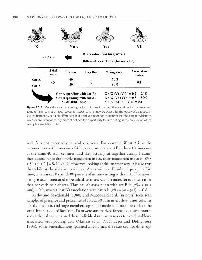
358 MACDONALD , STEWART, STOPKA , AND YAMAGUCHI
with A is not necessarily so, and vice versa. For example, if cat A is at theresource center 40 times out of 40 scan censuses and cat B is there 10 times outof the same 40 scan censuses, and they actually sit together during 8 scans,then according to the simple association index, their association index is [8/(8+ 30 + 0 + 2)] = 8/40 = 0.2. However, looking at this another way, it is also truethat while at the resource center cat A sits with cat B only 20 percent of itstime, whereas cat B spends 80 percent of its time sitting with cat A. This asym-metry is accommodated if we calculate an association index for each cat ratherthan for each pair of cats. Thus cat A’s association with cat B is [x/(x + ya +yab)] = 0.2, whereas cat B’s association with cat A is [x/(x + yb + yab)] = 0.8.
Kerby and Macdonald (1988) and Macdonald et al. (in press) took scansamples of presence and proximity of cats at 30-min intervals at three colonies(small, medium, and large memberships), and made ad libitum records of thesocial interactions of focal cats. Data were summarized for each cat each month,and statistical analyses used these individual summary scores to avoid problemsassociated with pooling data (Machlis et al. 1985; Leger and Didrichsons1994). Some generalizations spanned all colonies: the sexes did not differ sig-
Figure 10.5 Considerations in scoring indices of association are illustrated by the comings andgoing of farm cats at a resource center. Observations may be biased by the observer’s success inseeing them or by genuine differences in individuals’ attendance records, but the time for which thetwo cats are simultaneously present defines the opportunity for interacting in the calculation of theexample association index.

Measuring the Dynamics of Mammalian Societies 359
nificantly in their average monthly rate of presence, whereas age classes did;juvenile cats had the highest average monthly rate of presence, and adult malesthe lowest. Furthermore, each sex–age class displayed a favorite nearest-neigh-bor distance in terms of its tendency to maintain a given level of proximity toother cats (figure 10.6).
At the large colony, when kittens were within 1 m of an adult female, thiswas their mother on 71.1 percent and 58.3 percent of occasions for male andfemale kittens, respectively, whereas adult males tended to be within 1 m ofmale juveniles most frequently and of male kittens least frequently. Despitesuch generalizations, there were also significant differences in the pattern ofproximity between the colonies. For example, at the large colony, adult maleswere significantly more frequently within 1 m of adult females, but at themedium-sized colony no such tendency emerged. A further corollary of spatialstructure was that certain females occupied spatially peripheral positions,whereas others lived centrally, and the latter had significantly higher reproduc-tive success (figure 10.7).
Taking into account indices of association, it is possible to explore the fre-quency, rate, and quality at which cats interact. Take three cats, cat A spendingtwice as much time in the company of cat B as of cat C (figure 10.8). If A rubson B and C 40 and 8 times respectively, and attacks them 10 and 2 timesrespectively, then A rubs on and attacks B at only 2.5 times the rate at which itrubs on or attacks C, although A rubs and attacks B five times as often as C.The quality of A’s relationship with B and C is the same in that 80 percent ofits interactions with both are rubbing and 20 percent are attacking.
In reality, at Kerby and Macdonald’s (1988) large colony, individual centralmales averaged 602 (±254, SE) initiations relative to 502 (±142) for peripheralmales, but the latter were present so seldom that their hourly rate of interac-tion when present averaged 6.9 (±1.5), in comparison to the central males at2.3 (±0.7). The situation was opposite for females: Peripheral females inter-acted at low frequency, and when their presence was taken into account, theyinteracted at an even lower rate. Furthermore, in the context of grooming,Macdonald et al. (1987) showed that whereas the flow of licking differed sig-nificantly between pairs of interacting cats, it was invariably symmetric. Inmarked contrast, the flow of rubbing, though also differing between dyads,correlated with aggression but not grooming and was generally highly asym-metric. They concluded that in the society of female cats, rubbing as a measureof status flowed centripetally toward central dominant individuals; grooming,which was exchanged reciprocally, was a measure of social (and often genetic)alliances, but unrelated to status (figure 10.9).

Figure 10.6 Exploration of patterns of spatial proximity can reveal some unexpected structure towhat appears superficially to be a random gathering. In the case of farm cats, these graphs, basedon G. Kerby’s field study in Macdonald et al. (in press), reveal (A) that different age–sex classes ofindividuals positioned themselves at significantly different distances to their nearest neighbors and(B) that these positionings differed significantly depending on the age–sex class to which that neigh-bor belonged. AF = adult female, AM = adult male, JF = juvenile female, JM = juvenile male, KF =female kitten, KM = male kitten.
A
B

Measuring the Dynamics of Mammalian Societies 361
Figure 10.7 An ultimate goal of many ethological descriptions is to translate indices of socialbehavior into evolutionary consequences. In the case of Kerby and Macdonald’s (1988) and Mac-donald et al’s (in press) farm cat study, the spatial arrangement of female cats around the farmyardresource center was correlated with the number of kittens raised annually per female.
Macdonald et al.’s (1987, in press) and Kerby and Macdonald’s (1988) catstudy shows how even simple quantification can reveal unexpected layers ofstructure in unsophisticated mammalian societies.
In summary, to define social groups and to describe social dynamics onemust describe interactions that may be positive, tolerant, or negative in termsof their consequences for those involved. However, the choice of interactiontype, or of the way of quantifying it, may radically affect the researcher’s inter-pretation of the outcome. This should not surprise us. An analogy with humansocial dynamics shows us that very different patterns of interaction appear ifwe view exchange of such commodities as money, conversation, or affection.And the picture changes yet again if we look at frequency rather than quantityor quality of the exchange. The most pernicious problem lies in correct inter-pretation of the context of the interchange. Is the individual to which the mostmoney is observed to be given beloved kin, despised extortionist, or scarcelyknown shopkeeper?

362 MACDONALD , STEWART, STOPKA , AND YAMAGUCHI
Figure 10.8 The same observations of social interactions can be expressed in three ways: as thetotal flux of a given behavior pattern, as a rate, or as a proportion. In this case, the total frequency isgreater between A and B than between A and C (b > c), but qualitatively the components of theirrelationship are the same.
j Methods for Behavioral Measurement
Although our goal is not to provide an encyclopedic guide to the formidablepractical problems faced by the field biologist, we briefly review severalmethodologies relevant to measuring social dynamics.
IDENTIFYING THE INDIVIDUAL
From the variety of ways of identifying individuals reviewed by Stonehouse(1978), it is generally preferable to use natural characteristics. This necessitatesvalidation of identification skills and it is imperative that behavior is not inad-vertently used as a cue to identity. For scientific as well as ethical reasons, it isalso important to be alert to any influences of a marking technique on subse-quent behavior. For example, in an analysis of a new fur-clipping techniqueused to mark badgers for individual identification, Stewart and Macdonald(1997) assessed the effect of the clips on body condition using a matched-sam-ples test. Our concern was that the technique could cause thermoregulatorydisadvantage, and no significant effect of clipping on condition was found.Furthermore, marked individuals were capable of attaining high status in theirgroup, as measured among males by copulation frequency during female

Figure 10.9 (A) The flow of rubbing between a group of four cats studied by Macdonald et al.(1987) was much less than that of grooming, and the two differed in that rubbing relationshipstended to be highly asymmetric whereas grooming ones were symmetric. Furthermore, whereas theflow of grooming tended to mirror indices of association, those of rubbing and aggression did not, butthe latter two were correlated with each other but not with grooming. (B) Superimposed on these pat-terns, relationships were modified by kinship and age; for example, female 68 (in Kerby and Mac-donald’s [1988] large colony) interacted more with her sisters than her adult daughters, and morewith these 5 close kin than with the 12 other females available to her.
A
B

364 MACDONALD , STEWART, STOPKA , AND YAMAGUCHI
estrus. It is logically impossible to be certain that clip marks had no effect onbehavior, but as in the case of Hoogland’s (1995) Nyanzol dye-marked groundsquirrels, we could detect no evidence that it did. However, absence of evi-dence is not evidence of absence, so caution is necessary. For example, birdrings or ear tags have been demonstrated to affect judgments of asymmetryand mate choice in some species (Burley 1988). This topic is further discussedby Bekoff and Jamieson (1997) (see also Moehrenschlager et al. in press). In asimilar way, names of animals should be carefully chosen to avoid biasingbehavioral observation of social role. The name given to an animal, be it thatof a colleague, friend, or personality, can inadvertently influence all but themost objective observer. Even ascribing “male” and “female” names can causerecording biases. Numbers are better (although “A1” may still find deferentialrecording to “C5”), but can be rather hard to remember. In our own badgerstudy we primarily used names derived from the appearance of the identifyingfur clip mark, giving asexual and fairly connotation-free names such as Line,Dot, Dash, and Corners.
SAMPLING AND RECORDING RULES
Sampling rules dictate which subjects to watch and when. Martin and Bateson(1993) distinguish ad libitum, focal, scan, and behavior sampling. Recordingrules specify how the behavior is to be recorded. The two options are continu-ous recording and time sampling. Time sampling may be undertaken on aninstantaneous or one–zero basis.
The qualities of each sampling rule are easily envisaged through the eyes ofcontrasting onlookers at a football match. The typical spectator engages in adlibitum sampling and samples everything. He or she is likely to record thegoals and any spectacular fouls, with a bias toward the fouls committed by cer-tain star players and those committed on the ball. In contrast, a talent scoutmight be a focal sampler, observing one player at a time. He or she may gain apoor impression of the game as a whole, but a clear impression of the qualitiesof particular players. Of course, the scout must be alert to biases such as thestage of the match at which a given player becomes the focal subject (it wouldbe inappropriate to compare one player observed in the first 5 min withanother observed in the final 5 min). A team manager might opt for scan sam-pling, censusing the behavior of each player in turn, at rapid intervals, to getan overall impression of how the team functions as a unit. Finally, a gambler,interested only in the outcome of the game, may undertake behavior sampling,recording only goals. By focal or scan sampling one could miss these events.

Measuring the Dynamics of Mammalian Societies 365
Turning to recording rules, a continuous record contains the times atwhich each behavior started and ended, and thereby reveals true frequenciesand durations. Instantaneous sampling characterizes the current behavior atpredefined intervals. One–zero sampling records whether a behavior happenedin one particular interval of defined length. The most common combinationsare focal sampling with a continuous record, scan sampling with an instanta-neous record, and focal sampling with a one–zero record.
AD LIBITUM SAMPLING
An obvious bias in ad libitum sampling would arise if a researcher’s presump-tions led to particular individuals being disproportionately represented in thesample, thereby distorting their importance. This effect has been credited withthe overestimation of male roles in the societies of some primates and may sub-sequently have been countered by contrasting biases (Lindquist and Bernstein1987; Morell 1993). Furthermore, individuals or behavior patterns that areless conspicuous (because of short duration, subtlety, or association withobscured locations) tend to be underrepresented by ad libitum sampling. Forexample, Bernstein (1991) demonstrated that using ad libitum sampling ofrhesus monkeys (Macaca mulatta), the frequencies of contact aggression andavoidance were underestimated whereas that of chasing was overestimated. Arelated and insidious bias may affect the initial choice of study group. Sharmanand Dunbar (1982) noted that studies of baboon behavior tend to involvelarger than average groups. This erodes the generalizability of the resultsbecause the behavior of individuals was systematically influenced by the size ofthe group. In the same vein, perhaps the bias of primatologists’ expectationsfor their own taxon has lead to primates being described as having peculiarlycomplex social lives (Rowell and Rowell 1993). However, other taxa alsoemerge to have intricate societies, an obvious example being the Carnivora(Creel and Macdonald 1996). Despite this family of biases, ad libitum sam-pling can be useful during the naturalistic observation phase of pilot studiesand is valuable as an adjunct to more rigorous protocols that might otherwiseexclude important events that fell beyond their scope.
FOCAL SAMPLING
Because the whole attention of one observer is likely to be absorbed by onefocal subject, focal sampling risks losing valuable contextual and simultane-ously comparable information. The temptation to follow one focal individual

366 MACDONALD , STEWART, STOPKA , AND YAMAGUCHI
for longer than is necessary reduces the effective data set. Having observed afocal chimp for 300 hours, Kawanaka (1996) discovered that subsets of 25hours reliably and consistently represented the same time budget (see alsoArnoldmeeks and McGlone 1986). Excessive recording of particular focalindividuals also worsens the task of finding periods of relative stationarity.Cycling through a series of focal individuals and then checking an individualagainst itself in an earlier period may circumvent this. Video recording cansometimes relax these limitations. There may be a general warning in the find-ing of Arnoldmeeks and McGlone (1986) that focal animal sampling of oneindividual among a litter of young pigs provided a good measure of the timebudgets of other piglets in the same period for all but social behavior.
TIME SAMPLING
One–Zero Sampling
One–zero sampling consistently overestimates duration and gives unreliableinformation on frequency (Dunbar 1976; Altmann 1974). This can be partlyovercome by reducing the recording interval to periods shorter than the boutlength of the behavioral categories, but the technique then often becomesmore cumbersome than continuous focal sampling. Therefore, this oncecommon sampling method has largely been abandoned. Using a cumulativePoisson process, it is possible to assess, for a given interval length, the proba-bility that the necessary conditions will not be met for accurate frequencycounts and unbiased duration estimates in one–zero sampling (Suen and Ary1984; 1986a). Suen and Ary (1986b) also identified a post hoc correction pro-cedure that produces results with negligible systematic errors in one–zeroduration estimates. This correction procedure requires that more than five 0scores lie between two consecutive but not adjacent 1 scores (see also Quera1990).
Despite its general fall from favor, one–zero sampling has some potentialvirtues. It gives a measure of the probability that an observer will see at leastone example of the response in the specified time interval. Bernstein (1991)argues that this probability may be relevant to an animal’s perception: Forexample, when an individual is deciding whether to spend the next 5 min inthe vicinity of another individual, the probability of attack may be moreimportant than the mean duration or frequency of attacks. Martin and Bate-son (1993) also note that the onset, duration, and frequency of some behavior,such as play, are hard to represent with continuous sampling and hard to score

Measuring the Dynamics of Mammalian Societies 367
during true instantaneous sampling. The judgment that play has at leastoccurred in a previously defined interval is more likely to be accurate. Finally,some behavior, such as copulation, may occur often in one short interval andthen not be seen for many subsequent intervals. One–zero scan samplingreveals how long a researcher is likely to have to watch the animals to see aninstance of such behavior.
Instantaneous Scan Sampling
This technique scores what some or all individuals are doing at predeterminedtime intervals. It produces a reliable estimate of the total durations of activitiesthrough a dimensionless measure of the proportion of occasions during whichthe behavior is encountered (Hansson et al. 1993). Instantaneous scans maygive poor information on frequency, although this shortcoming is minimizedif the sample interval is small enough to catch even the shortest interveningperiod between recurrence (Odagiri and Matsuzawa 1994). However, as in thecase of short one–zero measures, such short bouts become more inconvenientthan focal sampling. Furthermore, the need for statistical independence of thedata points requires that sample intervals not be too short. For example, if 10successive scans all fell within a single long bout of a particular behavior, thenthey constitute a sample of 1, not 10. Such dependence would require that thedata be transformed to a proportion on an interval scale for comparison ratherthan being used as discrete categorical scores (and therefore could not be ana-lyzed in an interaction sociomatrix). As a rule, Bernstein (1991) suggests thatif the probability of scoring the same continuous state twice in succession isless than 0.05, then the two scans can be treated as independent. In practicethis means that the interval between scans should exceed the mean duration ofa state plus 1.96 standard deviations. Even long intervals between scans canprovide a basis for accurate estimates of mean time budgets, but the increase invariance caused by longer sampling intervals may swamp analyses of covaria-tion and produce type II errors (Poysa 1991).
The pros and cons of each approach, and the diverse aims of investigations,mean not only that no particular method is universally superior, but that evenfor one study an eclectic approach to sampling is likely to optimize data acqui-sition. A mix of all occurrence sampling, scan sampling, and focal individualinstantaneous sampling is possible. The results of all three are likely to beenhanced if decisions on the durations of intervals and focal sessions arejudged from preliminary analysis of a continuous focal sample (e.g., made byusing a portable video camera in the field).

368 MACDONALD , STEWART, STOPKA , AND YAMAGUCHI
TECHNIQUES FOR BEHAVIORAL MEASUREMENT
Simultaneous and continuous focal sampling of all individuals in a groupmight be the most accurate and informative combination of sampling andrecording, but circumstances may render this combination unattainable. Tech-nology is at hand to help. Computer-based event-recording software providesan automated string of actor, behavior (time), and modifiers (such as recipientof interaction and quality of interaction). Currently, memorizing the keyboardis the way to avoid taking one’s eyes off the subjects, but voice recognition soft-ware may soon allow input of data spoken in the correct syntax. Various soft-ware packages already assist behavioral recording, and the most sophisticated,such as Noldus Observer, offer a variety of tools for manipulation and basicstatistical analysis of the data and an easy Windows interface (Albonetti et al.1992; Noldus Information Technology 1995). Noldus also performs sequen-tial and nested analysis and allows simultaneous input from an alternative dig-itized source (e.g., heartbeat or external temperature).
Two caveats concern widespread adoption of sophisticated software. First,it may encourage a lazy uniformity in data acquisition that stifles innovationin sampling and recording rules or analyses. Second, a researcher’s new-foundability to record a plethora of behavior and contexts may exceed his or her abil-ity to frame hypotheses and manipulate and analyze the data.
There are circumstances under which video recording is an economicalalternative to direct observation and offers some unique advantages. The videorecord can be played and replayed, allowing multiple passes over complexsequences at a resolution of up to 50 frames per second. With a microphone,complex vocalizations can be spectrographically analyzed in context (Wong etal. 1999). The video and sound sequences may be digitized and stored using aPC and video capture board; this allows efficient indexed archiving of raw dataand use in electronically distributed ethograms. Video can also be time-codedand used with event recording packages to facilitate accurate data entry or evenallow automatic data entry for movement, interaction, and some simple pos-tural categories. Video can be used to calculate interobserver and intraobserverreliability, including the drift in ethogram categorization which often occurs inlong studies. Limited use of video in pilot studies can allow the disparitybetween different behavior sampling techniques and a true continuous recordto be assessed.
In automatic field use, video allows easy habituation for many species(including facility to use infrared light to provide illumination beyond thevisual range of most mammals). Continuous surveillance of multiple focal sitesbecomes a possibility for even a single researcher, with the equipment operat-

Measuring the Dynamics of Mammalian Societies 369
ing in conditions that would be too arduous for the researcher to endure forprotracted periods. Against these undoubted benefits video equipment canstill be initially costly, with problems of equipment reliability, accessibility, andsecurity. Video also has a more limited field of vision than a human observer,and because it requires transcription after the event, it may increase the dura-tion of studies. Stewart et al. (1997) describe the use and construction of auto-matic video surveillance units, and Wratten (1994) provides a general back-ground to video techniques.
Finally, although the naturalist’s preference may be to observe social behav-ior directly or with video, this may be uneconomical or unfeasible. Examplesof indirect measures include the frequencies of bite wounds (Woodroffe andMacdonald 1995a), chewing of ear tags (White and Harris 1994), and hunt-ing patterns from carcass retrieval ( Johnsingh 1983). Radiotracking has revo-lutionized the study of elusive mammals. Although initially used principally toplot movements, the use of radiotracking to supplement classic fieldcraft andas an aid to observation has long been advocated (Macdonald and Amlaner1980). It is also possible to infer features of social behavior from the dynamicinteraction between the movements of radiotracked individuals (Macdonaldet al. 1980; Doncaster 1990). The practicalities of radiotracking are reviewedin Kenward (1987) and analytical considerations in White and Garrot (1990).An increasing number of software packages for analyzing tracking data areavailable, such as Wildtrak (Todd 1992) and Ranges V.
j Analysis of Observational Data
Context must always have been important in human interpretation of thebehavior of other animals. Even our own aphorisms (blood’s thicker thanwater, do as you would be done by, and so on) reveal an intuition that presagesmodern conceptual insights regarding the forces fashioning animal societies,including our own. Today, biologists interpret behavior within a context forti-fied by theories of cognition, games, trait-group selection, kin selection, reci-procity, and byproduct mutualism. The traditional approach to observing ani-mals, with roots embedded in the Aristotelian idea of ascribing properties toanimals, could yield detailed ethograms that demonstrated the defining behav-ioral uniqueness of each species. Interspecific comparisons of these behaviorallexicons shed light on phylogenies even before the days of phylogenetic regres-sion (Tinbergen 1951). The quest for more robust tools with which to eluci-date the shared properties between species has, in the last 20 years, contributed

370 MACDONALD , STEWART, STOPKA , AND YAMAGUCHI
to the blurring of boundaries between studies of ecology, ethology, and socio-biology. Today, the basic questions posed by those concerned with the contex-tual interpretation of animal behavior still echo Niko Tinbergen’s (1963) fourfactors: causation, development, survival value, and evolution. The classicsequence starts with observation to document the behavioral repertoire in con-text, and this forms a basis for experimental study of causation, development,and survival value and an attempt to reconstruct the evolution of particularunits of behavior (McFarland 1981). The approach rests on parsimony andreductionism. Of course, there are different forms of reductionism, and thebiologist’s variant, as described by Konrad Lorenz in The Foundations of Ethol-ogy (1981), may deviate from the physicist’s method of general reduction.
Here, we consider some limitations of the rationales behind four conceptswidely used in the study of social dynamics: statistical rationality, matrix facil-ities, lag sequential and nested analysis, and concept of uncertainty measures(Markov chain analysis).
STATISTICAL RATIONALITY
A society is the product of social flux among its members and between themand outsiders. Therefore, for many purposes the description of a societyrequires quantification of the interactive components of behavior betweenmembers of, for example, a reproductive unit, group, colony, or population;these may be continuously or instantaneously recorded. In the analysis ofobservational data, insufficient attention to methodology can result in a riftbetween statistical significance and biological relevance, whereas the corre-spondence between these two can be fostered by attention to sampling tacticsand statistical sensitivity. An inadequately sensitive statistical method or modelmay fail to reveal the properties of an interactive behavior, even if an appro-priate sampling method was used.
The familiarity of two types of error has rendered neither rare. Type I errorinvolves mistaken rejection of a null hypothesis (i.e., a false positive); type IIerror is failure to reject a false null hypothesis (i.e., ignorance) (Lindgren1968). As a general statement, scientific validity depends partly on the sensi-tivity of the tests involved (decreasing the probability of type I errors) and onthe number of hypotheses tested (the accumulating building blocks of theargument adding to its objectivity and decreasing the probability of type IIerrors). However, there is a tradeoff between these kinds of error; decreasingtype I error can increase the risk of type II error (Shrader-Frachette and Mc-Coy 1992). There is also a risk that even when the hypothesis has been tightly

Measuring the Dynamics of Mammalian Societies 371
phrased, a test may pick up “departures” from H0 that result from “noise”rather than real differences. Matloff (1991) describes how confidence intervalanalysis may partly solve these problems. An advanced account of these topicsis given in Thompson (1992) and Krishnaiah and Rao (1988).
MATRIX FACILITIES: ANALYZING SEQUENTIAL DATA
A matrix is any rectangular array of numbers (e.g., frequencies, number oftransitions). If the array has r rows and s columns it is called an r by s (r × s)matrix. Thus for example,
a11 a12 a13a11 a12 a13
A (3 × 3) a21 a22 a23 and B (2 × 3)a21 a22 a23
a31 a32 a33
where each row can represent the actor entry and columns the receiver; that is,the value a11 represents frequency (or other value) of relations between therow descriptor (r1) and the column descriptor (s1).
Our task here is not to explain the mathematical principles of matrices (seeRoberts 1992), but to describe their uses in behavioral sciences. Interactionfrequencies among individuals, presented as a sociometric matrix, are often thebasis for analysis of social dynamics. Individuals are classed as actors or initia-tors in the rows (r) of the matrix and as receivers in the columns (s).
Other sociometric matrices include distance and association matrices; inthese, each cell contains a symmetric (dis)similarity measure for the pair of ani-mals indicated by the row and the column of the cell. The cells of a transitionmatrix contain the frequencies with which the behavior indicated by the row(the preceding behavior) is followed by the behavior indicated by the column(the succeeding behavior) (de Vries et al. 1993).
Relationships are often presented in terms of the dyadic interactionsbetween two individuals of the group. Frequencies of interactions within thedyad during defined time intervals are then written in sociometric matrices.These types of sociometric matrices are often used to identify the dominancehierarchy among individuals based on such key behavior patterns as initiatingaggression. One individual is defined as a dominant (the winner), the other asa subordinate (the loser). The strength of the relationship is expressed in termsof linearity (Appleby 1983). Han de Vries (1995) developed an improved testof linearity in dominance hierarchies containing unknown or tied relation-

372 MACDONALD , STEWART, STOPKA , AND YAMAGUCHI
ships. This test is based on Landau’s linearity index, but takes the unknownand tied relationships into account. An unknown relationship commonlyarises because two members of a dyad simply were not seen to interact. Thiscan occur for at least four reasons: sampling may be inappropriate, linearity ofthe dominance hierarchy may be an artifact of experimental circumstances(e.g., dispersal cannot occur in captivity), the formation of coalitions may leadto mutual protection or mutual avoidance, and linearity may not be a featureof the group’s social structure (ultimately because the ecological circumstancesoffer no selective advantage to linear dominance with regard to, for example,resource holding potential). However, papers acknowledging the first two cat-egories of problem are inevitably few.
The problems of elucidating a hierarchy and revealing its consequences areillustrated by wood mice (Apodemus sylvaticus). Although some aspects of thisspecies’ behavior can be studied in the wild (Tew and Macdonald 1994), theirsmall body size and large ranges thwart many studies and make them strongcandidates for observation in arenas (Plesner Jensen 1993) or seminaturalenclosures (Bovet 1972a, 1972b). Bovet (1972b) found that male wood miceof different statuses tended to be active at different times. Therefore, theyrarely met, which thwarts study of their encounters. Such problems can bepartly circumvented by the use of sociometric matrices. Because it illustratesthe use of matrices, we will go step by step through Stopka and Macdonald’s(in press) sociometric study of wood mice. Based on videotaped interactions ofnine mice observed over 3 months, the frequencies of transition between fightor chase and avoidance for all individuals in the colony were ranked (table10.1).
Each of these matrices can be analyzed for linearity in the relationshipsbetween the mice (a task swiftly performed by options in the package MATMAN).In the case of avoidance (table 10.1), this provides a statistic (Kendall’s linear-ity index K = 0.775), which indicates that the null hypothesis that avoidancerelationships are randomly distributed can be rejected in favor of the alterna-tive that they are linearly ordered (χ2 = 43.76, df = 20.16, p = 0.005). Similarlyfor allogrooming (K = 0.592), there is significant linearity (χ2 = 34.96, df =20.16, p = 0.03). However, linearity in avoidance relationships is stronger (p =0.005) than that in allogrooming relationships (p = 0.03), raising the possibil-ity that linearity in grooming merely reflects that in avoidance. The statisticaltool to test this hypothesis is the Kr row-wise matrix correlation test (de Vrieset al. 1993; de Vries 1995). When applied to the avoidance and allogroomingmatrices (in which the rows and columns are identically ordered), this reveals a

Measuring the Dynamics of Mammalian Societies 373
Table 10.1 Matrix of Frequencies of Transitions from Fight toAvoidance (top) and Frequencies of AllogroomingBehavior (bottom) Among Nine Wood Mice
Receiver (avoid)
M1 M2 M3 F1 F2 M4 F3 F 4 M5
M1 * 52 180 9 18 192 11 66 26M2 8 * 22 0 6 15 3 11 0M3 10 15 * 6 10 18 4 10 16F1 0 0 0 * 1 0 0 1 2
Actor (fight) F2 1 1 6 0 * 6 2 8 7M4 2 4 4 1 3 * 4 4 4F3 0 2 3 0 1 0 * 0 3F 4 5 3 5 0 4 3 0 * 1M5 0 0 1 0 0 0 0 0 *
Receiver
M1 M2 M3 M4 M5 F1 F2 F3 F 4
M1 * 1 0 3 0 62 15 124 13M2 0 * 0 0 0 6 3 8 6M3 0 0 * 0 19 4 2 14M4 1 0 0 * 0 4 1 8 4
Actor M5 0 0 0 0 * 0 0 0 0(groom) F1 6 1 2 2 0 * 0 1 3
F2 0 0 3 0 0 0 * 0 0F3 14 0 1 1 0 0 0 * 1F 4 1 1 0 0 0 1 0 0 *
From Stopka and Macdonald (submitted, b).
strong negative correlation (p-right = 0.941). Therefore, the dominance (avoid-ance) and grooming matrices exist independently. Tendencies to allogroom andavoid differ between males and females; in practice, lower-ranking males arerarely groomed and they avoid dominant males and are avoided by females,whereas females are the main recipients of grooming, which is mainly initiatedto them by dominant males. This pattern led us to conclude that in order toobtain matings, male wood mice have to groom females. This hypothesis is sup-ported by the positive row-wise correlations (p < 0.001), which reveal that malesthat are dominant and groom females most secure most copulations.

374 MACDONALD , STEWART, STOPKA , AND YAMAGUCHI
LAG SEQUENTIAL AND NESTED ANALYSIS
Sequential analysis facilitates study of the temporal structure of sequences ofevents. A common variant is lag sequential analysis, which involves calculatingfrequencies of transitions between pairs of events within a certain lag in a timeseries. The first event of each pair is called the criterion event (also calledantecedent, X-event, or given event) and the second event is the target event(also called the consequent or Y-event). Lag sequential analysis allows you toanswer questions such as “How many times is the (criterion) event Head Upfollowed by the (target) event Stare?” The time window in which the transitionfrom criterion to target event occurs is either a state lag or a time lag. In a state-lag sequential analysis, a transition is counted from a criterion event to the firsttarget event following this criterion event. In time-lag sequential analysis, atransition is counted from a criterion event to the target event occurringwithin a specified time window following the criterion event. All other eventsthat are not defined as either criterion or target events are ignored in the analy-sis. Lag-sequential analysis differs profoundly from other approaches (such aslog-linear models), which compare estimated expected frequencies withobserved frequencies because these do not have a sequential property. The onlyway to analyze changes of behavior through time is in terms of transitionsbetween the antecedent and the consequent behavior. Lag sequential analysisis currently the only method that applies a contextual approach: Instead ofanalyzing the frequencies of different behavior over a certain period of time,lag sequential analysis uses the frequencies of behavioral transitions (Roberts1992).
However, the results of lag sequential analysis are rarely expressed in termsof the absolute frequencies of transition from one event to the others; instead,they are often written in probabilistic terms as transition rates. The transitionrates, written in transition matrices, can be calculated from the frequencies oftransitions between preceding and consequent behavior using equation 1.6 inHaccou and Meelis (1992), which is formally written as a maximum likeli-hood estimator (MLE)—equation 10.1 or 10.2—when duration of an act isconstant:
αAB
= }N
NA
A
B} × }x
1
A
} (10.1)
or

Measuring the Dynamics of Mammalian Societies 375
αAB
= }N
NA
A
B
B
} (10.2)
where αA,B is the estimator of transition rates, NA,B is the number of transitionsfrom the state A to state B, NA is the number of states A, and xwA is the meanbout length of category A. MLE values are written in the state-space represen-tation (also known as flow diagrams), that is, a set of states and transition ratesbetween them.
In corroborative analyses at least two methods are currently used todescribe behavioral processes: multiple-matrix analysis and nested analysis.
Multiple-matrix analysis involves the construction of several matrices, oneeach for a variety of measurable parameters of social flux (e.g., dominance hier-archy, mutual grooming, approach and avoidance, acts of support, copula-tions, and paternity). The pattern of flow between individuals for each behav-ior pattern can then be compared between matrices using, for example,row-wise matrix correlation (association) or linearity indices (de Vries 1993).This approach provides answers to questions such as “Are dominant malesgroomed more frequently than subordinate males, or do females given protec-tion by other females reciprocate this support?” This can involve constructionof several matrices and row-wise correlations between them.
Nested analysis, on the other hand, involves defining questions withinmatrices. Subsets (nested categories) of data are selected within the overallmatrix. For example, a researcher might ask, “Is there a tendency for juvenilemales to be more successful in contests with rivals when positioned close totheir mothers?” To answer this, the researcher would analyze the outcomes offights when key individuals were adjacent to, or distant from, their mothers.
Both multiple matrix and lag sequential or nested analyses may involve themanipulation of very large data sets, and software is available to make this taskmore manageable. PC programs such as the Observer event recorder lagsequential analysis (Noldus 1994) and the MATMAN program (de Vries et al.1993) are designated for recording and analyzing such data.
SEARCHING FOR A BEHAVIORAL PATTERN (MARKOV CHAIN)
It is useful when analyzing sequential data to characterize the chance of onebehavior following another. If exclusive acts (events or states) in a sequence areindependent of each other, then the distribution of bout lengths will follow an

376 MACDONALD , STEWART, STOPKA , AND YAMAGUCHI
exponential distribution; such a sequence is said to have Markovian properties.Such a process is completely characterized by a set of transition rates, which arethe probabilities per unit of time of switching from one state to another. Bydefinition, acts within such a sequence are independent of each other and oftime. The termination rate of an act is constant (i.e., independent of the past)only if the duration of the bouts follows an exponential distribution. This factallows the inference of social interaction because dependencies between theterminations of different individuals would imply that they exchange signals(Haccou and Meelis 1992). Indeed, most sequences are not Markovianbecause the probability that most behaviors will occur depends on earlierevents in the sequence and other confounding variables. Generally, for a givenbehavior, the probability of occurrence of any future behavior in the sequenceis altered by additional knowledge concerning the past (Haccou and Meelis1992). The program UNCERT (Hailman and Hailman 1993) analyzes serialdependencies in sequential events using the method of Markov chains andexpressed in terms of the uncertainty that one event will follow another. Forexample, Hailman and Dzelzkalnz (1974) used Markov chain analyses toreveal that tail-wagging by mallard duck (Anas platyrhynchos) punctuated along sequence of behavior patterns, indicating that a display is about to start(loosely analogous to the role of a capital letter beginning a sentence).
PREDICTABILITY OF BEHAVIOR
Measures of uncertainty can be a valuable tool in assessing the predictability ofresponses of individuals to others. Again, we explore an example from ourwork on wood mice (Stopka and Macdonald, unpublished data). For example,all combinations of five male and four female wood mice kept under videosurveillance in an enclosure with abundant nest boxes sometimes denned com-munally, although there was no thermoregulatory need to huddle. It was there-fore surprising that cohabitants were often agonistic to each other. One of themost common categories of interaction was approach and nose-to-nose con-tact, categorized by Bovet (1972a, 1972b) as amicable, but lag sequentialanalysis revealed that although this (nose-to-nose) behavior pattern was indeedsometimes a precursor to flank-to-flank or nasoanal contact, on other occa-sions it was followed by attacking or chasing. Therefore, nose-to-nose encoun-ters are defined by their context within a sequence. Sequential analysis revealedthat nose-to-nose contact was sometimes the prelude to an amicable encounterand sometimes to an aggressive one (figure 10.10).
The crucial question is how to recognize mixed categories. Haccou and

Measuring the Dynamics of Mammalian Societies 377
Meelis (1992) recommend: performing a global inspection of bar plots toensure stationarity, testing the bout lengths of all acts in the ethogram forexponentiality (e.g., Darling’s test), using cumulative bout length plots and thelikelihood ratio change point test to reveal deviations from exponentialityattributable to lack of stationarity, and devising a rational basis (in the case ofnose-to-nose in wood mice, lag sequential analysis) on which to split prob-lematic categories into new robust categories. Other methods of splitting thebehavior according to the bouts are based on fitting a nonlinear curve to thelogarithm of the observed frequencies of gap lengths (Sibly et al. 1990) and onthe use of likelihood ratio tests in helping to determine whether the data occurin bouts (Langton et al. 1995).
However, it is important that the statistical procedure does not obscurebiological insight, so the new, split categories must make sense. For example,it is clearly sensible to split the instances of follow-B (individual B) that werepreceded by fight from those preceded by copulation or intromission becauseboth new categories of follow (A, B) have different contextual functions and,it turns out, different bout lengths. Splitting of the category nose-to-nose con-tact did not make sense because it was equally likely to precede a fight ornasoanal contact. However, on further exploration, the probability that nose-to-nose contact would lead to one or other of these categories depended heav-ily on the sex of interactant. Such sex-dependent sequences may even resolve
Figure 10.10 The flow diagram (state-space representation) of the sex-dependent nose-to-noseinteraction. Lines between behavioral elements represent the tendency of switching from one behav-ioral element to another, based on a maximum-likelihood estimator.

378 MACDONALD , STEWART, STOPKA , AND YAMAGUCHI
puzzles in video surveillance by allowing inference of the sex of an unmarkedindividual.
SEQUENCES THROUGH THE MIST
All animals are social, even if only to the extent of engaging in sexual repro-duction and otherwise avoiding each other. Understanding the rules that gov-ern social dynamics in general is a step to understanding our own lives (Axel-rod 1984). Everything happens in context, so it is unsurprising that weadvocate a contextual approach to studying society. Social relationships are theconsequences of entwining sets of events and states, and our aim has been toexplore how these may be disentangled through analyzing sequences ofchanges in time and space. Although some of these analytical approaches mayseem daunting through their unfamiliarity, they concern a phenomenon—sequentiality—that not only is at the root of life in the patterning of nucleicacids, but also suffuses every aspect of our daily experience in strings of wordsand sentences and stories. One story can be told in different ways for differentpurposes, just as an individual butterfly is expressed differently as larva, pupa,and imago. A metamorphosis in storytelling shows how the perceptions ofRobert Henryson, a fifteenth-century Scottish poet, might, for the purposes ofmeasuring the dynamics of mammalian society, be stripped to their essentials.In his Moral Fables, Henryson penned these words:
This country mouse lay flattened on the ground, fearing every minute thatshe would be killed; for her heart was pounding with strokes of fear, andfeverishly she trembled hand and foot. And when her sister found her insuch straits, for the sake of pity first she grieved a bit, then comforted herwith words as sweet as honey.
It is common for stories to be peppered with anthropomorphism, and oneclass of these, akin to mock anthropomorphism (Kennedy 1986), enrichesprose with insight. Certainly, understanding is not the sole prerogative of thosewho wield the colorless pen of late-twentieth-century science. On the otherhand, another class of anthropomorphism is blind to life’s processes and, in itsfancifulness, more often than not corrupts literature by diminishing under-standing. Stripping out these distractions is a step toward understanding, andinterpretation of the essence that remains hinges on the meaning of sequences,whether they be words or behaviors. In the contextual study of animal behav-ior the narration that precedes or succeeds a given action has equal weight to

Measuring the Dynamics of Mammalian Societies 379
the action itself. As a step toward such contextual analysis, we might wonderwhether Henryson had this in mind:
One rural female wood mouse (Apodemus sylvaticus) adopted a dorsoven-trally flattened posture, exhibiting, in an unspecified but seemingly fearfulcontext, tachycardia and elevated body temperature, and associated tremu-lous movements of the fore- and hind-paws. These signs appeared to bestress-induced. A conspecific female approached and initiated prolongednonreciprocal grooming, perhaps with the consequence of diminishing thesigns of putative stress. Subsequent molecular analyses confirmed thehypothesis that these individuals were siblings.
The only merit of the aridity of this version is that it exposes the states andevents that can usefully be defined in an ethogram and exposes the sequencesof those that will become grist for analysis:
(I) ETHOGRAM: crouch: dorsoventral flattened posture with head closeto the (i.e., modifier) ground; shake: tremulous movement of body (nomodifier), or shaking fore-paw(s) (modifier 1) or shaking hind-paw (mod-ifier 2); approach: one individual moves toward another; groom opposite:one individual grooms the other on the head, or neck, or back, or flank(modifier 1).
(II) SEQUENCE: BEHAVIOR: A-crouch → A-shake → B-approach-A→ B-nose-to-nose-A → B-groom-A.
MODIFIER 1: ground paw
MODIFIER 2: foot
TIME: t0 → t1 → t2 → t3 → t4 → . . . tn;;
DURATION: (t1 – t0) (t2 – t1) (t3 – t2) (t4 – t3) (tn – t4)
SUBJECTS: 2 female wood mice (Apodemus sylvaticus)
Clearly, there are many ways of describing an observation. Henryson’s orig-inal and our coded version may be quests for different sorts of understanding.The point is that having designed an ethogram and having chosen the correct

380 MACDONALD , STEWART, STOPKA , AND YAMAGUCHI
method of observation, we can distill an observed set of events or states into apattern that facilitates greater precision of interpretation and decreased risk offanciful anthropomorphism.
Acknowledgments
We are grateful to M. Dawkins, R. Dunbar, D. Johnson, and two anonymousreviewers for comments on an earlier draft. We also thank Luigi Boitani andTodd Fuller for their invitation to participate in the conference that spawnedthis book and for their forbearance as editors.
Literature Cited
Albonetti, M. E., J. Lazarus, D. W. Dickins, A. Whybrow, R. Schonheiter, J. Prenter, R.Elwood, J. D. Newman, F. O. Odberg, L. Kaiser, M. H. Pham-Delegue, V. Verguelen,J. C. Fentress, and M. L. Bocia. 1992. Software multiple review. The Observer: Soft-ware for behavioural research, version 2.0. Ethology, Ecology and Evolution 4: 401–414.
Altmann, J. 1974. Observational study of behaviour: Sampling methods. Behaviour 49:227–267.
Appleby, M. C. 1983. The probability of linearity in hierarchies. Animal Behaviour 32:600–608.
Arnoldmeeks, C. and J. J. McGlone. 1986. Validating techniques to sample behavior ofconfined, young-pigs. Applied Animal Behaviour Science 16: 149–155.
Axelrod, R. 1984. The evolution of co-operation. New York: Basic Books.Axelrod, R. and W. D. Hamilton. 1981. The evolution of cooperation. Science 211:
1390–1396.Barbault, R. 1988. Body size, ecological constraints, and the evolution of life-history strate-
gies. In M. K. Hecht, B. Wallace, and G. T. Prance, eds., Evolutionary biology, 261–285.New York: Plenum.
Bekoff, M. 1977. Quantitative studies of three areas of classical ethology: Social domi-nance, behavioural taxonomy, and behavioural variability. In B. Hazlett, ed., Quantita-tive methods in the study of animal behavior, 1–46. New York: Academic Press.
Bekoff, M. and D. Jamieson. 1997. Ethics and the study of carnivores: Doing science whilerespecting animals. In J. L. Gittleman, ed., Carnivore behavior, ecology and evolution,vol. 2, 15–45. Ithaca, N.Y.: Cornell University Press.
Berdoy, M., P. Smith, and D. W. Macdonald. 1994. Stability of social status in wild rats:Age and the role of settled dominance. Behaviour 132: 193–212.
Berger, J. and C. Cunningham. 1995. Predation, sensitivity and sex: Why female black rhi-noceroses outlive males. Behavioural Ecology 6: 57–64.
Bernstein, I. S. 1991. An empirical comparison of focal and ad-libitum scoring with com-mentary on instantaneous scans, all occurrence and one-zero techniques. AnimalBehaviour 42: 721–728.

Measuring the Dynamics of Mammalian Societies 381
Borries, C. 1992. Grooming site preferences in female langurs (Presbytis entellus). Interna-tional Journal of Primatology 13: 19–32.
Bovet, J. 1972a. On the social behaviour in a stable group of long-tailed field mice (Apode-mus sylvaticus). I. An interpretation of defensive postures. Behaviour 41: 43–54.
Bovet, J. 1972b. On the social behaviour in a stable group of long-tailed field mice (Apode-mus sylvaticus). II. Its relations with distribution of daily activity. Behaviour 41: 55–67.
Bressers, M., E. Meelis, P. Haccou, and M. Krok. 1991. When did it really start or stop: Theimpact of censored observations on the analysis of durations. Behavioural Processes 23:1–20.
Brown, J. L. 1975. The evolution of behaviour. New York: Norton.Burley, N. T. 1988. Wild zebra finches have band colour preferences. Animal Behaviour 36:
1235–1237.Cairns, S. J. and S. J. Schwager. 1987. A comparison of association indices. Animal Behav-
iour 35: 1454–1469.Chase, I. D. 1982. Dynamics of hierarchy formation: The sequential development of dom-
inance relationships. Behaviour 80: 218–240.Cheney, D. L. 1992. Intragroup cohesion and intergroup hostility: the relation between
grooming distributions and intergroup competition among female primates. Behav-ioural Ecology 3: 334–345.
Clout, M. N. and M. G. Efford. 1984. Sex differences in the dispersal and settlement ofbrushtail possums (Trichurus vulpecula). Journal of Animal Ecology 53: 737–749.
Clutton-Brock, T. H., F. E. Guinness, and S. D. Albon. 1982. Red deer: Behaviour and ecol-ogy of two sexes. Chicago: University of Chicago Press.
Clutton-Brock, T. H. and G. A. Parker. 1995. Punishment in animal societies. Nature 373:209–216.
Colgan, P. 1978. Quantitative ethology. New York: Wiley.Creel, S. 1997. Cooperative hunting and group size: Assumptions and currencies. Animal
Behaviour 54: 1319–1324.Creel, S. and D. W. Macdonald. 1996. Sociality, group size, and reproductive suppression
among carnivores. Advances in the Study of Behaviors 24: 203–257.Creel, S., S. L. Monfort, D. E. Wildt, and P. M. Waser. 1991. Spontaneous lactation is an
adaptive result of pseudopregnancy. Nature 351: 660–662.Cuthill, I. 1991. Field experiments in animal behaviour: Methods and ethics. Animal
Behaviour 42: 1007–1014.Dawkins, R. 1976. The selfish gene. Oxford, U.K.: Oxford University Press.Dawkins, R. 1989 (2d ed.). The selfish gene. Oxford, U.K.: Oxford University Press.Doncaster, C. P. 1990. Non-parametric estimates of interaction from radio-tracking data.
Journal of Theoretical Biology 143: 431–443.Drews, C. 1993. The concept and definition of dominance in animal behaviour. Behaviour
125: 283–313.Dugatkin, L. A. 1997. Cooperation among animals: An evolutionary perspective. Oxford,
U.K.: Oxford University Press.

382 MACDONALD , STEWART, STOPKA , AND YAMAGUCHI
Dunbar, R. I. M. 1976. Some aspects of research design and their implications in the obser-vational study of behaviour. Behaviour 58: 78–98.
Dunbar, R. 1988. Primate social systems. London: Croom Helm.Evans, P. G. H., D. W. Macdonald, and C. L. Cheeseman. 1989. Social structure of the
Eurasian badger (Meles meles): Genetic evidence. Journal of Zoology 218: 587–595.Fagen, R. M. 1978. Information measures: Statistical confidence limits and inference. Jour-
nal of Theoretical Biology 73: 61–79.Fagen, R. M. and R. N. Goldman. 1977. Behavioural catalogue analysis methods. Animal
Behaviour 25: 261–274.Faver, J., M. Mendl, and P. Bateson. 1986. A method for rating individual distinctiveness of
domestic cats. Animal Behaviour 34: 1016–1025.Findlay, C. S., R. I. C. Hansell, and C. J. Lumsden. 1989. Behavioural evolution and bio-
cultural games: Oblique and horizontal cultural transmission. Journal of TheoreticalBiology 137: 245–269.
Geffen, E., M. E. Gompper, J. L. Gittleman, H. K. Luh, D. W. Macdonald, and R. K.Wayne. 1996. Size, life-history traits, and social organization in the Canidae: A reeval-uation. American Naturalist 147: 140–160.
Geyer, L. A. and C. A. Kornet. 1982. Auto- and allo-grooming in pine voles (Microtus pine-torum) and meadow voles (Microtus pennsylvanicus). Physiology and Behavior 28: 409–412.
Ginsberg, J. R. and T. P. Young. 1992. Measuring association between individuals or groupsin behavioural studies. Animal Behaviour 44: 377–379.
Golani, I. 1976. Homeostatic motor processes in mammalian interactions: a choreographyof display. In P. P. G. Bateson and P. H. Klopfer, eds., Perspectives in ethology, vol. 2,69–134. New York: Plenum.
Golani, I. 1992. A mobility gradient in the organisation of vertebrate movement: The per-ception of movement through symbolic movement. Behavioural and Brain Sciences 15:249–266.
Goosen, C. 1987. Social grooming in primates. In G. Mitchell and J. Erwin, eds., Compar-ative primate biology, Vol. 2: Behaviour, cognition, and motivation, 107–131. New York:Alan R. Liss.
Haccou, P. and E. Meelis. 1992. Statistical analysis of behavioural data. Oxford, U.K.:Oxford University Press.
Haccou, P. and E. Meelis. 1995 (2d ed.). Statistical analysis of behavioural data. Oxford,U.K.: Oxford University Press.
Hailman, J. P. and J. J. I. Dzelzkalns. 1974. Mallard tail-wagging: Punctuation for animalcommunication? American Naturalist 108: 236–238.
Hailman, E. D. and J. P. Hailman. 1993. UNCERT software (beta version) user’s guide.http://www.cisab.indiana.edu/CSASAB/index.html ([email protected]).
Hansson, L. 1992. Fitness and life history correlates of weight variations in small mammals.Oikos 64: 479–484.
Hansson, M. B., L. J. Bledsoe, B. C. Kirkevold, C. J., Casson, and J. W. Nightingale. 1993.

Measuring the Dynamics of Mammalian Societies 383
Behavioural budgets of captive sea otter mother–pup pairs during pup development.Zoo Biology 12: 459–477.
Hare, J. F. 1992. Colony member discrimination by juvenile Columbian ground squirrels(Spermophilus columbianus). Ethology 92: 301–315.
Harris, S. and P. C. L. White. 1992. Is reduced affiliative rather than increased agonisticbehaviour associated with dispersal in red foxes? Animal Behaviour 44: 1085–1089.
Hazlett, B. A. 1977. Quantitative methods in the study of animal behaviour. New York: Aca-demic Press.
Hemelrijk, C. K. 1990. Models and tests of reciprocity, unidirectionality and other socialinteraction patterns at group level. Animal Behaviour 39: 1013–1029.
Hemelrijk, C. K. and A. Ek. 1991. Reciprocity and interchange of grooming and supportin captive chimpanzees. Animal Behaviour 41: 923–935.
Herrera, E. A. and D. W. Macdonald. 1989. Resource utilisation and territoriality in group-living capybaras (Hydrochoerus hydrochaeris). Journal of Animal Ecology 58: 667–679.
Herrera, E. A. and D. W. Macdonald. 1993. Aggression, dominance, and mating successamong capybara males (Hydrochoerus hydrochaeris). Behavioural Ecology 4: 114–119.
Hinde, R. A. H. 1981. Social relationships. In D. McFarland, ed., The Oxford companion toanimal behaviour, 521–527. Oxford, U.K.: Oxford University Press.
Hinde, R. A., ed. 1983. Primate social relationships. An integrated approach. Oxford, U.K.:Blackwell Scientific.
Hofer, H. and M. East. 1993. Loud calling in a female-dominated mammalian society. IIBehavioural contexts and functions of whooping of spotted hyaenas, Crocuta crocuta.Animal Behaviour 42: 651–669.
Hoogland, J. L. 1995. The black tailed prairie dog: Social life of a burrowing mammal.Chicago: University of Chicago Press.
Iacobucci, D. 1990. Derivation of subgroups from dyadic interactions. Psychological Bul-letin 107: 114–132.
Johnsingh, A. J. T. 1983. Large mammalian prey-predators in Bandipur. Journal of the Bom-bay Natural History Society 80: 1–53.
Jouventin, P. and A. Cornet. 1980. The sociobiology of pinnipeds. Advances in the Study ofBehavior 11: 121–141.
Kawanaka, K. 1996. Observation time and sampling intervals for measuring behavior andinteractions of chimpanzees in the wild. Primates 37: 185–196.
Kennedy, J. S. 1986. Some current issues in orientation to odour sources. In T. L. Payne, M. C. Birch, and C. E. J. Kennedy, eds., Mechanisms in insect olfaction, 11–25. Oxford,U.K.: Clarendon.
Kenward, R. 1987. Wildlife radio-tagging. London: Academic Press.Kerby, G. and D. W. Macdonald. 1988. Cat society and the consequences of colony size. In
D. Turner and P. Bateson, eds., The domestic cat: The biology of its behaviour, 67–81.Cambridge, U.K.: Cambridge University Press.
Kraft, B., C. Colin, and P. Peignot. 1994. Diving-for-food: A new model to assess socialroles in a group of laboratory rats. Ethology 96: 11–23.

384 MACDONALD , STEWART, STOPKA , AND YAMAGUCHI
Krebs, J. R., and N. B. Davies. 1991 (3d ed.). Behavioural ecology. Oxford, U.K.: BlackwellScientific.
Krishnaiah, P. R. and T. J. Rao. 1988. The handbook of statistics. Amsterdam: Elsevier.Kruuk, H. 1972. The spotted hyena. Chicago: Chicago University Press.Kruuk, H. 1978. Foraging and spatial organisation of the badger (Meles meles). Behavioural
Ecology and Sociobiology 4: 75–89.Langton, S. D., D. Collet, and M. R. Sibly. 1995. Splitting behaviour into bouts; a maxi-
mum likelihood approach. Behaviour 132: 9–10.Ledger, D. W. and I. A. Didrichsons. 1994. An assessment of data pooling and some alter-
natives. Animal Behaviour 48: 823–832.Lehner, P. N. 1996 (2d ed.). Handbook of ethological methods. Cambridge, U.K.: Cambridge
University Press.Lindgren, B. W. 1968. Statistical theory. London: Macmillan.Lindquist, T. and I. S. Bernstein. 1987. A feminist perspective on dominance relationships
in primates. American Journal of Primatology 12: 355.Lindstedt, S. L., B. J. Miller, and S. W. Buskirk. 1986. Home range, time, and body size in
mammals. Ecology 67: 413–418.Lorenz, K. 1981. The foundations of ethology. New York: Springer-Verlag.Lott, D. F. 1991. Intraspecific variation in the social systems of wild vertebrates. Cambridge,
U.K.: Cambridge University Press.Macdonald, D. W. 1983. The ecology of carnivore social behaviour. Nature 301: 379–384.Macdonald, D. W. 1981. Dwindling resources and the social behaviour of capybaras
(Hydrochoerus hydrochaeris). Journal of Zoology 194: 371–391.Macdonald, D. W. 1995. Wildlife rabies: The implications for Britain. Unresolved ques-
tions for the control of wildlife rabies: Social perturbation and interspecific interac-tions. In Rabies in a changing world, 33–48. Cheltenham: British Small Animal Veteri-nary Association.
Macdonald, D. W. and C. J. Amlaner, Jr. 1980. A practical guide to radio tracking. In C. J.Amlaner and D. W. Macdonald, eds., A handbook on biotelemetry and radiotracking,143–159. Oxford, U.K.: Pergamon.
Macdonald, D. W., P. J. Apps, G. Carr, and G. Kerby. 1987. Social behaviour, nursing coali-tions and infanticide in a colony of farm cats. Advances in Ethology 28: 1–66.
Macdonald, D. W., F. G. Ball, and N. G. Hough. 1980. The evaluation of home range sizeand configuration using radio-tracking data. In D. W. Macdonald and C. J. Amlaner,eds., A handbook on biotelemetry and radio tracking, 143–159, 405–426. Oxford, U.K.:Pergamon.
Macdonald, D. W. and G. M. Carr. 1989. Food security and the rewards of tolerance. In V.Standen and R. A. Foley, eds., Comparative socioecology: The behavioural ecology ofhumans and other mammals, 75–99. Oxford, U.K.: Blackwell Scientific.
Macdonald, D. W. and O. Courtenay. 1996. Enduring social relationships in a populationof crab-eating zorros, Cerdocyon thous, in Amazonian Brazil. Journal of Zoology 239:329–355.

Measuring the Dynamics of Mammalian Societies 385
Macdonald, D. W., N. Yamaguchi, and G. Kerby. In press (2d ed.). Group-living in thedomestic cat: Its sociobiology and epidemiology. In D. Turner and P. Bateson, eds., Thedomestic cat: The biology of its behaviour. Cambridge, U.K.: Cambridge University Press.
Machlis, L. 1977. An analysis of the temporal patterning of pecking in chicks. Behaviour63: 1–70.
Machlis, L., P. W. D. Dood, and J. C. Fentress. 1985. The pooling fallacy: Problems arisingwhen individuals contribute more than one observation to the data set. Zeitschrift fürTierpsychologie 68: 201–214.
Martin, P. and P. Bateson, eds. 1993 (2d ed.). Measuring behaviour: An introductory guide.Cambridge, U.K.: Cambridge University Press.
Matloff, N. S. 1991. Statistical hypothesis testing: Problems and alternatives. Environmen-tal Entomology 20: 1246–1250.
May, R. M. 1975. Patterns of species abundance and diversity. In M. L. Cody and J. Dia-mond., eds., Ecology and evolution of communities, 81–120. Cambridge, Mass.: HarvardUniversity Press.
McFarland, D. J. 1981. The Oxford companion to animal behaviour. Oxford, U.K.: OxfordUniversity Press.
McKnight, B. L. 1995. Behavioural ecology of hand reared elephants (Loxodonta africana)in Tsavo East National Park, Kenya. African Journal of Ecology 33: 242–256.
Milinski, M. and G. A. Parker. 1991 (3d ed.). Competition for Resources. In J. R. Krebsand N. B. Davies, eds., Behavioural ecology: An evolutionary approach, 137–168.Oxford, U.K.: Blackwell Scientific.
Mitchell, B. W., N. S. Thompson, and H. L. Miles, eds. 1997. Anthropomorphism, anecdotesand animals. New York: State University of New York Press.
Moehrenschlager, A., D. W. Macdonald, and C. Moehrenschlager. In press. The effects oftrapping and handling swift foxes. In L. Carbyn and M. Sovoda, eds., Swift fox biology.Edmonton, Alberta: Canadian Circumpolar Institute.
Morell, V. 1993. Primatology: Seeing nature through the lens of gender. Science 260:428–429.
Moser, R., M. Cords, and H. Kummer. 1991. Social influences on grooming site prefer-ences among captive long-tailed macaques. International Journal of Primatology 12:217–230.
Noe, R., C. P. van Schaik, and J. A. R. A. M. van Hoof. 1991. The market effect: Anexplanation for pay-off asymmetries among collaborating animals. Ethology 87: 97–118.
Noldus Information Technology. 1994. The Observer, support package for video tape analysis.Reference manual, Version 3.0. Wageningen, the Netherlands: Noldus Information Tech-nology.
Noldus Information Technology. 1995. The Observer, base package for Windows. Referencemanual, Version 3.0. Wageningen, the Netherlands: Noldus Information Technology.
Odagiri, K. and Y. Matsuzawa 1994. Application of an instantaneous sampling method tolamb’s play behaviour. Japanese Journal of Animal Psychology 43: 9–16.

386 MACDONALD , STEWART, STOPKA , AND YAMAGUCHI
Packer, C. and T. Caro. 1997. Foraging costs in social carnivores. Animal Behaviour 54:1317–1324.
Pearl, M. C. and S. R. Schulman. 1983. Techniques for the analysis of social structure inanimal societies. Advances in the Study of Behavior 13: 107–146.
Plesner Jensen, S. 1993. Temporal changes in food preferences of wood mice (Apodemus syl-vaticus L.). Oecologia 94: 76–82.
Pollock, G. B. 1994. Social competition or correlated strategy? Evolutionary Ecology 8:221–229.
Poysa, H. 1991. Measuring time budgets with instantaneous sampling: A cautionary note.Animal Behaviour 42: 317–318.
Quera, V. 1990. A generalised technique to estimate frequency and duration in time sam-pling. Behavioral Assessment 12: 409–424.
Roberts, B. A. 1992. Sequential data in biological experiments. An introduction for researchworkers. London: Chapman & Hall.
Rogers, L. M., C. L. Chesseman, and S. Langton. 1997. Body weight as an indication ofdensity-dependent population regulation in badgers (Meles meles) at Woodchester Park,Gloucestershire. Journal of Zoology 242: 597–604.
Romanes, G. J. 1881. Nature, Oct. 27, 604.Roper, T. J. 1992. Badger (Meles meles) sett architecture, internal environment and func-
tion. Mammal Review 22: 43–53.Rowell, T. E. and C. A. Rowell. 1993. The social organization of feral Ovis aries ram groups
in the pre-rut period. Ethology 95: 213–232.Rubenstein, D. I. 1993. The ecology of female social behaviour in horses, zebras and asses.
Physiology and Ecology Japan 29: 13–28.Schino, G., F. Aureli, and A. Troisi. 1988. Equivalence between measures of allogrooming:
an empirical-comparison in 3 species of macaques. Folia Primatologica 51: 214–219.Schleidt, W. M., G. Yakalis, M. Donnelly, and J. McGarry. 1984. A proposal for a standard
ethogram, exemplified by an ethogram of the bluebreasted quail (Coturnix chinensis).Zeitschrift für Tierpsychologie 64: 193–220.
Seyfarth, R. M. 1983. Grooming and social competition in primates. In R. A. Hinde, ed.,Primate social relationships, 182–190. Oxford, U.K.: Blackwell Scientific.
Sharman, M. and R. I. M. Dunbar. 1982. Observer bias in selection of study group inbaboon field studies. Primates 23: 567–573.
Shrader-Frachette, K. S. and E. D. McCoy. 1992. Statistics, costs and rationality in ecolog-ical inference. Trends in Ecology and Evolution 7: 96–99.
Sibley, R. M., H. M. R. Nott, and D. J. Fletcher. 1990. Splitting behaviour into bouts.Animal Behaviour 39: 63–69.
Sillero-Zubiri, C., P. J. Johnson, and D. W. Macdonald. 1998. A hypothesis for breedingsynchrony in Ethiopian wolves (Canis simensis) Journal of Mammalogy 79: 853–858.
Smuts, B. 1985. Sex and friendship in baboons. New York: Aldine.Stevenson-Hinde, J. 1983. individual characteristics and the social situation. In R. A.
Hinde, ed., Primate social relationships, 28–35. Oxford, U.K.: Blackwell Scientific.

Measuring the Dynamics of Mammalian Societies 387
Stewart, P. D. 1997. The social behaviour of the European badger (Meles meles). Doctoral the-sis. Oxford, U.K.: Oxford University Press.
Stewart, P. D., S. A. Ellwood, and D. W. Macdonald. 1997. Video surveillance of wildlife:An introduction from experience with the European badger (Meles meles). MammalReview 27: 185–204.
Stewart, P. D. and D. W. Macdonald. 1997. Age, sex, and condition as predictors of moultand the efficacy of a novel fur clip technique for individual marking of the Europeanbadger (Meles meles). Journal of Zoology 241: 543–550.
Stonehouse, B. 1978. Animal marking: Recognition marking of animals in research. Balti-more, Md.: University Park Press.
Stopka, P. and D. W. Macdonald. 1998. Signal interchange during mating in the woodmouse (Apodemus sylvaticus): The concept of active and passive signalling. Behaviour135: 231–249.
Stopka, P. and D. W. Macdonald. 1999. The market effect in the wood mouse, Apodemussylveticus: Selling information on reproductive status. Ethology 105: 913–1008.
Suen, H. K. and D. Ary. 1984. Variables influencing one–zero and instantaneous time sam-pling outcomes. Primates 25: 89–94.
Suen, H. K. and D. Ary. 1986a. Poisson cumulative probabilities of systematic errors insingle-subject and multiple subject time sampling. Behavioural Assessment 8: 155–169.
Suen, H. K. and D. Ary. 1986b. A post hoc correction procedure for systematic errors intime sampling duration estimates. Journal of Psychopathology and Behavioral Assessment8: 31–38.
Swinton, J., F. Tuyttens, D. W. Macdonald, D. J. Nokes, C. L. Cheeseman, and R. Clifton-Hadley. 1997. A comparison of fertility control and lethal control of bovine tuberculo-sis in badgers: The impact of perturbation induced transmission. Philosophical Transac-tions of the Royal Society of London B352: 619–631.
Taber, A. B. and D. W. Macdonald. 1992. Communal breeding in the mara Dolichotispatagonium. Journal of Zoology 227: 439–452.
Tew, T. E. and D. W. Macdonald. 1994. Dynamics of space use and male vigour amongstwood mice, Apodemus sylvaticus, in the cereal ecosystem. Behavioral Ecology and Socio-biology 34: 337–345.
Thierry, B., C. Gauthier, and P. Peignot. 1990. Social grooming in Tonkean macaques(Macaca tonkeana). International Journal of Primatology 11: 357–375.
Thompson, S. K. 1992. Sampling. New York: Wiley.Tinbergen, N. 1951. The study of instinct. Oxford, U.K.: Oxford University Press.Tinbergen, N. 1963. On aims and methods in ethology. Zeitschrift für Tierpsychologie 20:
410–433.Todd, I. A. 1992. Wildtrak: Non-parametric home range analysis for the Macintosh. Oxford,
U.K.: Isis Innovations.Tuyttens, F. A. M. and D. W. Macdonald. In press. Social perturbation caused by popula-
tion control: Implications for the management and conservation of wildlife. In M.

388 MACDONALD , STEWART, STOPKA , AND YAMAGUCHI
Gosling, W. Sutherland, and M. Avery, eds., Behaviour and conservation. Cambridge,U.K.: Cambridge University Press.
de Vries, H., W. J. Netto, and L. H. Hanegraaf. 1993. MATMAN: A program for the analy-sis of sociometric matrices and behavioural transition matrices. Behaviour 125:157–175.
de Vries, H. 1993. The rowwise correlation between two proximity matrices and the partialrowwise correlation. Psychometrica 58: 53–69.
de Vries, H. 1995. An improved test of linearity in dominance hierarchies containingunknown or tied relationship. Animal Behaviour 50: 1375–1389.
de Waal, F. B. M. 1992. Coalitions as part of reciprocal relations in the Arnhem chimpanzeecolony. In A. H. Harcourt and F. B. M. de Waal, eds., Coalitions and alliances in humansand other animals, 233–258. Oxford, U.K.: Oxford University Press.
White, G. C. and R. A. Garrott. 1990. Analysis of wildlife radio-tracking data. London: Aca-demic Press.
White, P. C. L. and S. Harris. 1994. Encounters between red foxes (Vulpes vulpes): Implica-tions for territory maintenance, social cohesion and dispersal. Journal of Animal Ecology63: 315–327.
Wilson, E. O. 1975. Sociobiology. Cambridge, Mass.: Belknap.Wong, J., P. D. Stewart, and D. W. Macdonald. 1999. Vocal repertoire in the European
badger (Meles meles): Structure, context, and function. Journal of Mammalogy 80:570–588.
Woodroffe, R. 1993. Alloparental behaviour in the European badger. Animal Behaviour 46:413–415.
Woodroffe, R. and D. W. Macdonald. 1993. Badger sociality: Models of spatial grouping.Symposium of the Zoological Society of London 65: 145–169.
Woodroffe, R. and D. W. Macdonald. 1995a. Costs of breeding status in the Europeanbadger (Meles meles). Journal of Zoology 235: 237–245.
Woodroffe, R. and D. W. Macdonald. 1995b. Female–female competition in Europeanbadgers (Meles meles): Effects on breeding success. Journal of Animal Ecology 64: 12–20.
Wrangham, R. W. 1974. Artificial feeding of chimpanzees and baboons in their naturalhabitat. Animal Behaviour 22: 83–93.
Wratten, S. D., ed. 1994. Video techniques in animal ecology and behaviour. London: Chap-man & Hall.

Chapter 11
Modeling Species Distribution with GISFabio Corsi, Jan de Leeuw, and Andrew Skidmore
From the variety of checklists, atlases, and field guides available around theworld it is easy to understand that distribution ranges are pieces of informationthat are seldom absent in a comprehensive description of species. Their usesrange from a better understanding of the species biology, to simple inventoryassessment of a geographic region, to the definition of specific managementactions. In the latter case, knowledge of the area in which a species occurs isfundamental for the implementation of adequate conservation strategies.Conservation is concerned mostly with fragmentation or reduction of the dis-tribution as an indication of population viability (Maurer 1994), given that,for any species, range dimension is considered to be correlated to populationsize (Gaston 1994; Mace 1994).
Unfortunately, animals move and this poses problems in mapping theiroccurrence. Traditional methods used to store information on species distri-butions are generally poor (Stoms and Estes 1993). Distributions have beendescribed by drawing polygons on a map (the “blotch”) to represent, withvarying approximations, a species’ ranges (Gaston 1991; Miller 1994). Theaccuracy of the polygons relies on the empirical knowledge of specialists andencloses the area in which the species is considered likely to occur, althoughthe probability level associated with this “likelihood” is seldom specified. Amore sophisticated approach divides the study area into subunits (e.g., admin-istrative units, equal-size mesh grid), with each subunit associated with infor-mation on the presence or absence of the species. In this case the distributionrange of a species is defined by the total of all subunits in which presence isconfirmed; however, blank areas are ambiguous as to whether the species isabsent or no records were available (Scott et al. 1993).

390 CORS I , D E LEEUW, AND SK IDMORE
New approaches tend to overcome the concept of distribution range andmove toward one of area of occupancy.1 This concept is particularly useful forconservation action and has therefore been included in the new iucnRed Listcriteria (iucn1995). In this chapter we outline the basis of identifying distri-butions that represent a step toward the definition of a real area of occupancy.
For example, imagine a biologist who needs to find zebras. Intuitively, theodds of finding zebras in Scandinavia are very low, but moving to Kenyagreatly increases the odds. This process is based on very basic assumptions suchas that zebras live in warm places, say, with an average annual temperature of13–28°C. Obviously our observer won’t expect to find zebras in every place onEarth that has an average annual temperature of 13–28°C; there are manyother ecological requirements, along with other reasons, such as historical con-straints (see Morrison et al. 1992 for a review) and species behavioral patterns(Walters 1992), that contribute to define the distribution of the zebra. Never-theless, if our biologist extends the same process, taking into account the pre-ferred ranges of values of various environmental variables, the probability offinding the species in the areas in which these preferences are simultaneouslysatisfied increases.
If the aim of our researcher is to map the areas in which the species is mostlikely to be found rather than to find an individual, the entire process can beseen as a way of describing the species’ presence in terms of correlated envi-ronmental variables. And if inexpensive and broadly acquired environmentaldata (e.g., vegetation index maps derived from satellite data) are used to definespecies probability of presence, then maps of species distribution can be pro-duced quickly and efficiently.
To provide a formal approach to species distribution modeling, the processcan be divided into two phases. The first phase assesses the species’ preferredranges of values for the environmental variables taken into account, and thesecond identifies all locations in which these preferred ranges of values are ful-filled. The first phase is generally called habitat suitability index (hsi) analysis,habitat evaluation procedures (hep) (Williams 1988; Duncan et al. 1995), or,more generally, species–environment relationship analysis. The second, whichinvolves the true distribution model, has seen its potential greatly enhanced inthe last 10 years by the increasing use of geographic information systems (GIS),which can extrapolate the results of the first phase to large portions of territory.
The power of GIS resides in its ability to handle large amounts of spatialdata, making analysis of spatial relationships possible. This increases the num-ber of variables that can be considered in an analysis and the spatial extent towhich the analysis can be carried out (Burrough 1986; Haslett 1990).

Modeling Species Distribution with GIS 391
Thus GIS provides a means for addressing the multidimensional nature ofthe species–environment relationship (Shaw and Atkinson 1990) and the needto integrate large portions of land (eventually the entire biosphere) into theanalysis (Sanderson et al. 1979; Klopatek et al. 1983; Flather and King 1992;Maurer 1994) to produce robust conservation oriented models.
This chapter is a review of models and methods used in GIS-based speciesdistribution models; it is based on a literature review carried out on GEOBASE2
with the following keywords: GIS, remote sensing (RS), wildlife, habitat, and dis-tribution. The 82 papers collected were classified according to the main toolused (GIS or RS), the modeling approach, the analysis technique, the discussionof the assumptions, and the presence of a validation section. At the same time,information was gathered on the use of the term habitat, the number of vari-ables used for modeling, and the kind of output produced.
Far from being comprehensive, the review was the starting point for a ten-tative classification of GIS distribution models that is presented in this chapter;at the same time, it allowed us to focus attention on some issues that we con-sider among the most important for correct use of GIS in species distributionmodeling. In fact, although it offers powerful tools for spatial analysis, GIS hasbeen largely misused and still lacks a clear framework to enable users to exploitits potential fully.
These issues range from unspecified objectives in the process of modelbuilding to the lack of adequate support for the assumptions underlying themodels themselves. A large part of the chapter is devoted to the problem of val-idation, which we believe is crucial throughout the process of model buildingbut is very seldom taken into account.
Before discussing these issues, we address the problem of terminologyinconsistencies, which has a much broader extent in ecology than the specificrealm of species distribution modeling. The problem emerges from our reviewand is probably caused, in this context, by misleading use of the same term inthe different disciplines that have come to coexist under the wide umbrella of GIS.
j Terminology
Multidisciplinary fields of science are very appealing because they bringtogether people with different experience and backgrounds whose constructiveexchange of ideas may generate new solutions. In fact, many solutions thathave been successfully developed and used in one field of science may, with

392 CORS I , D E LEEUW, AND SK IDMORE
minor changes, be used in other fields. The very nature of GIS makes it essen-tial that specialists in different scientific disciplines contribute to the generaleffort of setting up and maintaining common data sets.
One drawback is that in the early phases of tool development (such as GIS),people who master the new tool tend to become generalists, invading otherfields of science without having the necessary specific background. This maycause problems both in the solutions provided, which generally tend to be toosimplistic, and in terminology, because the same term or concept can be usedwith slightly different meanings in different disciplines. This is the case, forinstance, with use of the concept of scale. For the cartographer, large scale per-tains to the domain of detailed studies covering small portions of the earth’ssurface (Butler et al. 1986), whereas for the ecologist large scale means anapproach that covers regional or even wider areas (Edwards et al. 1994). Obvi-ously this derives from the fact that cartographers use scale to mean the ratiobetween a unit measure on the map and the corresponding measure on theearth’s surface, whereas the ecologist uses it in the sense of proportion orextent. For example, the relationship between the geographic scale and theextension of ecological studies supplied by Estes and Mooneyhan (1994) high-lights that large scale in ecology is often associated with small geographic scale:
Site = 1:10,000 or larger
Local = 1:10,000 to 1:50,000
National or regional = 1:50,000 to 1:250,000
Continental = 1:250,000 to 1:1,000,000
Global = 1:1,000,000 or smaller
In ecology it would be better to use the adjectives f ine or broad (Levin 1992),which places the term scale more in the context of its second meaning.
If the confusion arising from the two uses of large scale seems trivial (at leastfrom the ecologists’ point of view), we believe that the different uses that havebeen made of the word habitat give rise to major misunderstandings and thusneed to be clarified (Hall et al. 1997).
j Habitat Definitions and Use
The term habitat 3 forms a core concept in wildlife management and the dis-tribution of plant and animal species. The fact that the actual sense in which it

Modeling Species Distribution with GIS 393
is used is rarely specified suggests that its meaning is taken for granted. How-ever, Merriam-Webster’s dictionary (1981) provides two different definitionsand Morrison et al. (1992) observed that use of the word habitat remains farfrom unambiguous. The latter distinguished two different meanings: one con-cept that relates to units of land homogeneous with respect to environmentalconditions and a second concept according to which habitat is a property ofspecies.
Our literature review provided us with a variety of definitions and uses ofthe term habitat that are wider than the dichotomy suggested by Morrison etal. (1992). We arranged these various meanings according to two criteria:whether the term relates to biota (either species and or communities) or toland, and whether it relates to Cartesian (e.g., location, such as a positiondefined by a northing and easting) or environmental space (e.g., the environ-mental envelope defined by factors such as precipitation, temperature, andland cover) (table 11.1).
Although the classification in table 11.1 allows us to partition the differentdefinitions of habitat we have traced, in reality this partition is rather hazy. Forinstance, definitions range from the place where a species lives (Begon et al.1990; Merriam-Webster 1981; Odum 1971; Krebs 1985), which is a totallyCartesian space–related concept, to the environment in which it lives (Collin1988; Moore 1967; Merriam-Webster 1981; Whittaker et al. 1973). In thislast case habitat is seen as a portion of the environmental space. At bothextremes of the range of definitions, the slight differences in the terms usedallows us to define a continuous trend between the Cartesian and the environ-mental concept, which is further supported considering a few definitions thatcombine the Cartesian and the environmental space (Morrison et al. 1992;Mayhew and Penny 1992). These last authors define habitat as the area thathas specific environmental conditions that allow the survival of a species. Notethat all of these definitions relate habitat to a species and some describe it as aproperty of an organism.
With a similar range of definitions, another group relates habitat to bothspecies and communities. For instance, Zonneveld (1995:26), in accordancewith a Cartesian concept, defined it as “the concrete living place of an organ-ism or community.” Others relate it to both Cartesian and environmentalspace, defining it as the place in which an organism or a community lives,including the surrounding environmental conditions (Encyclopaedia Britan-nica 1994; Yapp 1922).
All of the definitions cited so far defined habitat in terms of biota. Zon-neveld (1995) remarked that the term habitat may be used only when specify-ing a species (or community). Yet habitat has been used as an attribute of land.

394 CORS I , D E LEEUW, AND SK IDMORE
Table 11.1 Classification Scheme of the Term Habitat
Biota Land
SpeciesSpecies
and Communities
Cartesian space Begon et al. (1990) Zonneveld (1995)Krebs (1985)Odum (1971)Merriam-Webster
(1981)Cartesian
space and Morrison et al.
(1992)Encyclopaedia
Britannica (1994)Stelfox and
Ironside (1982)environment Mayhew and
Penny (1992)Yapp (1922) Kerr (1986)
USFWS
(1980a, 1980b)Herr and Queen
(1993)Environment Collin (1988)
Merriam-Webster(1981)
Whittaker et al.(1973)
Moore (1967)
The various meanings of habitat are grouped according to whether the term relates to biota (species orspecies and communities) or land and whether it relates to Cartesian space, environmental space, orboth.
Riparian habitat, for instance, is a specific environment, with no relation tobiota. Use of habitat in this sense is widespread in the ecological literature (e.g.,old-forest habitat, Lehmkuhl and Raphael [1993], or woodland habitat,Begon et al. [1990]). The concept predominates in ecology applied to landmanagement such as habitat mapping (Stelfox and Ironside 1982; Kerr 1986),habitat evaluation (USFWS 1980a, 1980b; Herr and Queen 1993), and habi-tat suitability modeling (USFWS 1981). A similar meaning of habitat is usedin a review of habitat-based methods for biological impact assessment (Atkin-son 1985). Although it has been used very often in this sense, we were unableto find a single definition. A closely related concept, the habitat type, which isused in habitat mapping, has been defined as “an area, delineated by a biolo-gist, that has consistent abiotic and biotic attributes such as dominant or sub-

Modeling Species Distribution with GIS 395
dominant vegetation” (Jones 1986:23). Daubenmire (1976) noted that thismeaning of habitat type corresponds to the land unit concept (Walker et al.1986; Zonneveld 1989). In articles dealing with habitat evaluation, the term isused in a similar sense.
The use of an ambiguous term leads to confusion in communicationbetween scientists. The ambiguity of habitat is also observed within the samepublication. Lehmkuhl and Raphael (1993), for instance, simultaneously used“old-forest habitat” and “owl habitat.” Even ecological textbooks are not freefrom ambiguity. Begon et al. (1990:853) defined habitat as “the place where amicro-organism, plant or animal species lives,” suggesting that they considerhabitat a property of a species. However, when outlining the differencebetween niche and habitat, they later described habitat in terms of a land unit(Begon et al. 1990:78): “a woodland habitat for example may provide nichesfor warblers, oak trees, spiders and myriad of other species.” Confusion ariseswith respect to habitat evaluation as well. When defined as a property of aspecies, unsuitable habitat does not exist because habitat is habitable by defi-nition. In this case some land may be classified as habitat and all of this is suit-able. When defined as a land property, all land is habitat, whether suitable orunsuitable, for a specific species.
Why is the term habitat used in these various senses? The word originatesfrom habitare, to inhabit. According to Merriam-Webster (1981) the term wasoriginally used in old natural histories as the initial word in the Latin descrip-tions of species of fauna and flora. The description generally included the envi-ronment in which the species lives. This leads to the conclusion that habitatwas originally considered a species-specific property. It is interesting to notethat the definitions we traced originated both from ecology and geography,suggesting that the confusion was not the result of separate developments intwo fields of science.
At some time habitat started to be used as a land-related concept, mostlikely in conjunction with habitat mapping. A possible explanation for thechange is given by Kerr (1986), who remarked that mapping habitat4 individ-ually for each species would be an impossible job. He argued that a map dis-playing habitat types and describing the occurrence of species in each typewould be more useful to the land manager. This suggests that the land-relatedhabitat concept arose because it was considered more convenient to map habi-tat types rather than the habitat of individual species.
We suggest that there was a second reason for the popularity of habitat typemaps. In general the distribution of species is affected by more than one envi-ronmental factor. Until a decade ago it was virtually impossible to display

396 CORS I , D E LEEUW, AND SK IDMORE
more than one environmental factor on a single map. The habitat type,defined as a mappable unit of land “homogeneous” with respect to vegetationand environmental factors, circumvented this problem and was the basis of theland system (land concept) maps developed in the 1980s (Walker et al. 1986;Zonneveld 1989). However, it is based on the assumption that environmentalfactors show an interdependent change throughout the landscape and that theenvironmental factors are constant within the “homogeneous” area. Thus to acertain extent the land unit meaning of the term habitat arose as a way to over-come operational difficulties in species distribution mapping. Nevertheless,given that the variation of one environmental factor affecting the distributionof a species often tends to be independent of the other environmental factors,homogeneity is seldom the case, so there is seldom a true relationship betweenspecies and habitat types.
The advent of GIS has made it possible to store the variation of environ-mental factors independently and subsequently integrate these independentenvironmental surfaces into a map displaying the suitability of land as a habi-tat for a specific species.
The first examples of such GIS-based habitat mapping were published in thesecond half of the 1980s (e.g., Hodgson et al. 1988). Since then there has beena steady increase of the number of GIS-based habitat models (figure 11.1). Theincrease illustrates a move away from the general habitat-type mapping appli-cable for multiple species toward more realistic species-specific habitat maps.
At the same time, the habitat type loses its usefulness because of thedecreasing need to classify land in homogeneous categories. In other words,species-specific habitat mapping is increasingly incorporating independentenvironmental databases processed using information on the preferences ofthe species concerned. In view of the anticipated move toward species-specifichabitat models, we prefer to use the original species-related concept of habitatinstead of a land-related concept; to avoid confusion, in this chapter we willuse the terms species–environment relationships and ecological requirements in-stead of the terms species habitat and habitat requirements.
j General Structure of GIS-Based Models
The rationale behind the GIS approach to species distribution modeling isstraightforward: the database contains a large number of data sets (layers), eachof which describes the distribution of a given measurable and mappable envi-ronmental variable. The ecological requirements of the species are defined

Modeling Species Distribution with GIS 397
Figure 11.1 Percentage of the papers dealing with habitat modeling using no spatial information,RS, GIS, and a combination of RS and GIS for three periods (1980–1985, 1986–1991, and 1992–1996).
according to the available layers. The combination of these layers and the sub-sequent identification of the areas that meet the species’ requirements identifythe species’ distribution range, either actual (if there is evidence of presence) orpotential (if the species has never been observed in that area).
This basic scheme can be implemented using different approaches. A fewclassifications based on different criteria have been attempted. For example,Stoms et al. (1992) classified models based on the conceptual method used todefine the species–environment relationship, whereas Norton and Possingham(1993) based their classification on the result of the model and its applicabil-ity for conservation. Accordingly, Stoms et al. (1992) classified GIS species dis-tribution models into two main groups—deductive and inductive—whereasNorton and Possingham (1993) gave a more extensive categorization of mod-eling approaches.
We have tried to define logical frameworks that can be used to classifyspecies distribution models based on the major steps that must be followed tobuild them. To this end, we find the deductive–inductive categorization themost suitable starting point because it focuses attention on the definition ofthe species–environment relationship, which is the key point for the imple-mentation of distribution models.

398 CORS I , D E LEEUW, AND SK IDMORE
The deductive approach uses known species’ ecological requirements toextrapolate suitable areas from the environmental variable layers available inthe GIS database. In fact, analysis of the species–environment relationship isrelegated to the synthesizing capabilities and wide experience of one or morespecialists who decide, to the best of their knowledge, which environmentalconditions are the most favorable for the existence of the species. Once thepreferences are identified, generally some sort of logical (Breininger et al.1991; Jensen et al. 1992) or arithmetic map overlay operation (Donovan et al.1987; Congalton et al. 1993) is used to merge the different GIS environmentallayers to yield the combined effect of all environmental variables.
When the species–environment relationships are not known a priori, theinductive approach is used to derive the ecological requirements of the speciesfrom locations in which the species occurs. A species’ ecological signature canbe derived from the characterization of these locations. Then, with a processthat is very similar to the one used in deductive modeling but is generally moreobjectively driven by the type of analysis used to derive the signature, it is usedto extrapolate the distribution model (Pereira and Itami 1991; Aspinall andMatthews 1994).
In figure 11.2 we summarize the data flow of GIS-based species distributionmodels for both the deductive and the inductive approaches. Whereas in thedeductive approach GIS data layers enter the analysis only to create the distri-bution model, in the inductive approach they are used both to extrapolate thespecies–environment relationship and the distribution model. Along with thedata flow, the steps that need validation are also evidenced in the figure. Vali-dation is addressed in more detail later in this chapter, but it is interesting tonote here that validation procedures are needed at many different stages in theflow diagram.
Both inductive and deductive models can be further classified according tothe kind of analysis performed to derive the species–environment relationship.Essentially these can be subdivided into two main categories: the descriptiveand the analytical. Models pertaining to the first category use either the spe-cialists’ a priori knowledge (deductive–descriptive) or the simple overlay ofknown location of the species with the associated environmental variable lay-ers (inductive–descriptive) to define the species–environment relationship.Descriptive models generally are based on very few environmental variable lay-ers, most often just a single layer. They tend to describe presence and absencein a deterministic way; each value or class of the environmental variable is asso-ciated with presence or with absence (e.g., the species is known to live insavanna with an annual mean temperature of 15–20°C, so savanna polygons

Modeling Species Distribution with GIS 399
Figure 11.2 General data flow of the two main categories of GIS species distribution models identi-fied in this chapter.
falling within the adequate temperature range are to be included as suitableenvironments). No attempt is made to define confidence intervals to the indi-vidual estimate, nor is any information provided on the relative importance ofone variable over another (e.g., vegetation types vs. temperature). Moreover,no estimate of the degree of association or its variability is provided with therelationship.
On the other hand, models that fall into the analytical group introducevariability in the sense that advice from different specialists is combined todefine species–environment relationships, thus introducing variability interms of different opinions of the experts (deductive–analytical), or that thespecies observation data are analyzed in a way that takes into account the rangeof acceptability of all environmental variables measured, their confidence lim-its, and their correlation. Both the deductive–analytical and the inductive–analytical approaches tend to estimate the relative importance of the differentenvironmental layers considered in the analysis, thus moving toward an objec-tive combination of environmental variable layers.
Examples of deductive–analytical models are based on techniques such asmulti-criteria decision-making (MCDM) (Pereira and Duckstein 1993), Delphi(Crance 1987), and nominal group technique (NGT) (Allen et al. 1987).Generally speaking, these techniques use the advice of more than one special-

400 CORS I , D E LEEUW, AND SK IDMORE
ist as independent estimates of the “true” species–environment relationshipand evaluate its variability based on these estimates.
Inductive–analytical techniques rely on samples of locations that are ana-lyzed with some sort of statistical procedure. Different techniques have beenused, including generalized linear models (GLMs; McCullagh and Nelder 1988;for applications see Akçakaya et al. 1995; Bozek and Rahel 1992; Pausas et al.1995; Pearce et al. 1994; Pereira and Itami 1991; Thomasma et al. 1991; VanApeldoorn et al. 1994), Bayes theorem approach (Aspinall 1992; Aspinall andMatthews 1994; Pereira and Itami 1991; Skidmore 1989a), classification trees(Walker 1990; Walker and Moore 1988; Skidmore et al. 1996), and multi-variate statistical methods such as discriminant analysis (Dubuc et al. 1990;Flather and King 1992; Haworth and Thompson 1990; Livingston et al.1990; Verbyla and Litvaitis 1989), discriminant barycentric analysis (Genardand Lescourret, 1992), principal component analysis (PCA) (Lehmkuhl andRaphael 1993; Picozzi et al. 1992; Ross et al. 1993), cluster analysis (Hodgsonet al. 1987), and Mahalanobis distance (Clark et al. 1993; Knick and Dyer1997; Corsi et al. 1999).
Models that use simple univariate statistics, such as ANOVA, Pearson rankcorrelation, and Bonferroni, pertain to a different subgroup because theseanalyses do not generally allow for definition of the relative importance of theenvironmental variables.
Further differences should be outlined for models that rely on the interpo-lation of density or census estimates to extrapolate distribution patterns.Although we have included these models in the inductive–analytical group,the geostatistical approach (Steffens 1992) on which they are generally basedsuggests putting them into a slightly different subgroup.
Finally, another means of classifying GIS distribution models can be basedon their outputs. Essentially, these can be distinguished as categorical–discretemodels and probabilistic–continuous models. Most often the products of thefirst type of models are polygon maps in which each polygon is classified accord-ing to a presence–absence criterion or a nominal category (e.g., frequent, scarce,absent). The products of the second type of model are continuous surfaces ofan index that describes species presence in terms of the relative importance ofany given location with respect to all the others. Indices that have been used arethe suitability index (Akçakaya et al. 1995; Pereira and Itami 1991), probabil-ity of presence (Agee et al. 1989; Skidmore 1989a; Aspinall 1992; Clark et al.1993; Walker 1990), ecological distances from “optimum” conditions (Corsi etal. 1999), and species densities (Palmeirin 1988; Steffens 1992). All theseindices can be mapped as a continuous surface throughout the species range.
Modeling Species Distribution with GIS 401
Generally, discrete models are built associating the presence of a species topolygons of land unit types (e.g., vegetation categories), most often with adeductive approach; in fact, transferring into the realm of GIS, the traditionalway of producing distribution maps is based on a similar but more arbitrarypartitioning of the study area (e.g., administrative boundaries, regular grids;see also “Habitat Definitions and Use”). There are also some examples ofbinary classifications of continuous environmental variables (e.g., slope,aspect, elevation) using statistical techniques such as logistic regression (Pereiraand Itami 1991) or discriminant analysis (Corsi et al. 1999). Categorical–dis-crete models do not account for species mobility and tend to give a staticdescription of species distribution. Nevertheless, this approach can be used toaddress the problem of defining areas of occupancy (Gaston 1991) and thuscan be used successfully for problems of land management and administra-tion. On the other hand, probabilistic models can describe part of the stochas-ticity typical of locating an individual of a species and can be used to addressproblems of corridor design and metapopulation modeling (Akçakaya 1993),introducing the geographic dimension in the analysis of species viability.
LITERATURE REVIEW
Table 11.2 indicates the results of our bibliographic review. Papers are classi-fied according to the categories described in the previous paragraph.
We have considered GIS and RS as two different views of the same tool, theformer being more devoted to spatial correlation analysis and the later moreconcerned with basic data production. In fact, the two families of softwaretools share many basic functions and are evolving toward integration into asingle system. It should be noted that the review includes not only papers thatuse GIS or RS but also some that deal with HSI, HEP and general assessment ofspecies’ ecological requirements. The papers in this last group do not generallyrepresent examples of spatial models (Scott et al. 1993), in the sense that theirproducts are not distribution maps, but they have been included because theyare considered to be just a few steps away from a real distribution model. Infact, they describe the ecological requirements of the species in terms of map-pable environmental conditions.
Most of the papers that use the deductive approach consider the a prioriknowledge sufficient to define the ecological requirements of the species underinvestigation. This is especially true of papers that model distribution on thebasis of interpretation of remotely sensed data; in fact, 15 out of 16 papers per-taining to the deductive group that used remotely sensed data to model species

402 CORS I , D E LEEUW, AND SK IDMORE
Table 11.2 Classification of Reviewed Papers
Deductive
Descriptive GIS GIS
and RS
RS Non-spatial
GIS GIS
and RS
RS Non-spatial
9 8 7 8 32 3 1 0 0 4 36Analytical GIS GIS and
RS
RS Non-spatial
GIS GIS
and RS
RS Non-spatial
3 0 1 4 8 14 4 4 16 38 4640 42
Papers are classified according to the approach used to define the species–environment relationship andwhether their approach was descriptive or analytical. Further subtopics indicate whether the authorconsiders the research to pertain to the domain of RS, GIS, or both. Nonspatial is used for papers that donot contain an explicit distribution model but define species–environment relationship in terms ofmappable variables.
Inductive
distributions fall within the descriptive group. In these papers, image classifi-cation techniques tend to receive more emphasis, whereas the ecological appli-cation is most often seen as an excuse to apply a specific classification algorithm.
The time trend of the papers published shows rather stable use of RS tech-nology and increasing use of GIS. Up to 1986, no paper makes explicit referenceto the term GIS, even though some of the papers dealing with the use of RS douse raster GIS-style overlay procedures to define their distribution models (e.g.,Lyon 1983) and others do use a spatial approach but do not mention GIS (e.g.,Mead et al. 1981).
Little is generally said about model assumptions. Of the 82 papersreviewed, only 21 discuss their assumptions. Those that do generally limittheir discussion to the statistical assumptions of the technique used to performthe analysis. Very few deal with the biological and ecological assumptions andtend to take them for granted. When dealing with ecological modeling, weneed to take into account both biological and methodological assumptions,along with some general assumptions that may limit the applicability of theresults produced (Starfield 1997).
Validation, a step that is evidenced at different levels in the data flow dia-gram (figure 11.2), is generally limited to the accuracy of the result of theanalysis (e.g., distribution map); nothing is said about the accuracy of the orig-inal data sets (e.g., GIS data layers, observation locations) and no considerationis given to issues such as error propagation in GIS overlay (Burrough 1986).
Only 15 papers validate of the accuracy of their results based on an inde-

Modeling Species Distribution with GIS 403
pendent estimate of the distribution (either through comparison with an inde-pendent set of observations or through comparison with the known distribu-tion of the species); interestingly, 50 percent of these papers are based on the de-ductive approach. In fact, it should be noted that because observation data setsare the most expensive data to be collected within the general framework of set-ting up a GIS species distribution model, the deductive approach is the most cost-effective if seen from the validation point of view. In fact, to avoid bias, a modeldeveloped with an inductive approach cannot be validated using the same dataset used to derive the species–environment relationship. Thus validation can beperformed either with a second, independent data set or by dividing the origi-nal data set into two subsets, one of which is used to derive species–environmentrelationships and the other to validate the resulting model.
Finally, it is interesting to note that the multidimensional power of GIS is stillnot backed up by adequate quantity and quality of geographic data sets (Stomset al. 1992). This is reflected in the number of environmental variables used inanalysis. In the papers reviewed, the average is just below 4.8, and only 9 out of82 analyze more than 9 environmental variables, whereas 23 papers base theirdistribution models on only one environmental variable, generally vegetation.
j Modeling Issues
Based on the results of the literature review, we have identified five major issuesthat must be addressed to allow a sound GIS modeling of species distributions.These range from uncertainties in the objectives of the research to the lack ofadequate support for the assumptions underlying the implementation of GIS
models. A problem that is gaining awareness is that of scale, in both time andspace, but it still suffers from inadequate tools.
Slightly different is the issue of data availability, which is rarely addressableby the biologist concerned with species distribution modeling but limits thetype of models that can be developed.
Finally, a review of sources of errors and ways of estimating the accuracy ofa GIS model addresses the problem of validation.
CLEAR OBJECTIVES
When setting up an ecological model, the very first step to be considered isclear statement of the model’s objective (Starfield 1997). There is great confu-sion about the objectives of many published papers. This may caused byoverqualification of the tool, in the sense that use of the tool becomes the

404 CORS I , D E LEEUW, AND SK IDMORE
objective of the paper, or by uncertainty in defining the model’s goals, alongwith coexisting purposes of predicting or understanding (Bunnell 1989). Forinstance, most of the papers based on the inductive approach deal with the def-inition of a species–environment relationship without specifying whether theyintend to analyze the relationship of cause and effect or just use the relation-ship as a functional description of the effect. In the first case, the goal would beto evidence the limiting factors that are related to the species’ biological needsand that drive the distribution process; in the second, it would be the simpleuse of correlated variables whose distribution is functional to the descriptionof the species’ distribution.
Basically, we can summarize species needs as food, shelter, and adequatereproduction sites (Flather et al. 1992; Pausas et al. 1995). When using the dis-tribution of an environmental variable to describe the species’ distribution weimplicitly assume that there is a correlation between these basic needs and theenvironmental variables used. This correlation can be causal; that is, itdescribes the species’ basic needs. In such cases we can identify a function thatwithin a reasonable range of values associates each value of the environmentalvariable to a measure of the fulfillment of the species’ basic needs (e.g., repro-ductive success). But it can also be a functional description; that is, we don’treally know why some ranges of values of the environmental variable are pre-ferred by the species but we observe that the species tends to occur more fre-quently within those ranges. The variable might influence all the species’ basicneeds simultaneously or be correlated to another variable that describes one ofthe species’ needs.
Generally speaking, the quantity and quality of the locational data and theGIS layers used in analyses are not sufficient to assess cause–effect relationshipsthat determine the species’ distribution. Furthermore, cause–effect relation-ships spring from the interactions of biophysical factors that range throughdifferent time and space scales (Walters 1992); few papers take scale depen-dency into account in their analysis. Moreover in this kind of analysis causaleffects can be hidden by independent interfering variables (Piersma et al.1993) or by the unaccounted stochasticity of natural events such as weatherfluctuations, disturbance, and population dynamics (Stoms et al. 1992) andshould be assessed in controlled environments.
We believe such uncertainties could be addressed by defining the overall goalas the assessment of the relationship that best describe the species distribution.In other words, even if the causal understanding of a relationship is not clear,whenever the species–environment relationship is able to describe the distribu-tion of a species satisfactorily, the overall goal is achieved (Twery et al. 1991).

Modeling Species Distribution with GIS 405
Obviously the approach just described has some drawbacks. Without anadequate description of the cause–effect relationship between the species andenvironmental variables, models lose in transferability, in both space and time,and this limits their predictive capabilities (Levin 1992).
ASSUMPTIONS
All models analyzed extrapolate their results to an entire study area on theassumption of space independence of the phenomenon observed at a givenplace. That is, in the case of both a deductive and an inductive approach, thespecies–environment relationship is built on evidence that a certain speciesoccurs somewhere and that we know the values of the environmental variablesat those locations. Obviously we know only that a species occurs at locationswhere it has been observed, only part of these locations have measurements ofthe environmental variables, and usually these measurements are collected onlyfor the limited time range during which the investigation was carried out. Thus,when building distribution models, evidence collected in a portion of the rangeis extrapolated to the entire range of occurrence of a species. In order to do so,it is assumed that the species–environment relationship used to build the modelis invariant in space and time. Most of the time this is not the case, especiallyfor species with a wide range and for generalist species. In fact, the higher thevariance of the species–environment relationship, the higher the number oflocations required to provide an adequate ecological profile for the species.
Second, it is generally implicitly assumed that variables that are notincluded in the analysis have a neutral effect on the results of the model. Thatis, we need to assume either that the species’ ecological response to these envi-ronmental variable is constant or that the response is highly correlated with theother variables included.
Even though both of these general assumptions are very difficult to test, webelieve that they should be discussed on a case-by-case basis because the resultof their violation is species-specific. Errors may be negligible in certain casesbut can introduce major interpretation problems in other cases.
Biological assumptions
Biological assumptions are direct consequences of the general assumptions dis-cussed in the previous paragraph. We nevertheless believe that they are proba-bly the most critical, but have received minimal attention in the literature.
The first assumption, which follows from the general assumption of space

406 CORS I , D E LEEUW, AND SK IDMORE
and time independence, states that observations reflect distribution. In otherwords, information on absence can be derived from observation data (Rexstadet al. 1988; Clark et al. 1993), which is obviously seldom the case. In fact, anytime we have a record for a species we can be sure that the species (at least occa-sionally) occurs at that location. In contrast, if there is no observation for aspecies, we can only assume that we have a record of absence if there is no biasin our sampling scheme and that we have conducted our observations over asufficiently long period. Even then we have no way of evaluating the randomeffects that are intrinsic in observing animals.
These assumptions can have statistical relevance in dealing with induc-tive–analytical approaches, but must hold true also for the deductive models.If there is a constant bias in the visibility of a species’ individuals, for instancebecause part of their range is less accessible than others to researchers and thuscannot be as carefully investigated, the species–environment relationship re-flects this bias. For instance, observation data are often gathered through sight-ings carried out by volunteers (Stoms et al. 1992; Hausser 1995), which do notfollow a predefined (e.g., random) sampling scheme. Habitat cover may limitobservations to areas where the species is visible (Agee et al. 1989). This maycreate an artificial response curve that associates a positive relationship to thevalues of the environmental variables measured in the locations where thespecies is more visible and a negative one in the ones measured in areas werethe species has been less investigated. In such cases, we would end up mappingthe areas where the species and the observers are most likely to meet, not thetrue distribution of the species.
This example is tailored to inductive–analytical models but can easily beextended to deductive ones, both descriptive and analytical, considering thatthe deductive approach is based on the a priori knowledge of specialists whorely on series of observations to gain experience and define the species–envi-ronment relationship. Again, these observations can suffer from accessibilityor visibility biases.
A further assumption is that observations reflect the environmental selec-tion of the species. Obviously this is not always true; for example, occurrencesof migrant or vagrant individuals whose presence in a given location is occa-sional may be considered among observations. An extreme case is representedby locust swarms blown into the middle of the desert by strong winds. Clearly,their presence does not reflect any ecological preference. Nevertheless, if weconsider only the observation per se, we would conclude that high densities oflocusts are found in the desert and that locusts do prefer (with all the limita-tions that this term carries along in such an analysis) desert environments.

Modeling Species Distribution with GIS 407
Obviously the strong wind of the example should be regarded as a stochasticevent and thus be treated as an outlier in the definition of a possible GIS distri-bution model. In other words, observations should be analyzed for their con-tent of unconstrained selection by the species.
We will see, when dealing with the issues of scale, that GIS distributionmodels tend to describe only the deterministic components that drive aspecies’ distribution pattern, so stochastic events must be either averaged onthe long term or eliminated as outliers. When observations are carried out fora limited time and the biology of the species under investigation is scarcelyknown, this problem can become increasingly important because the identifi-cation of outliers will be virtually impossible.
Statistical assumptions
Most of the statistical techniques used to define species–environment relation-ships rely on the identification of two observation sets: one that identifies loca-tions in which the species is present and one in which it is absent. Even thoughthis cannot be identified properly as a statistical assumption, it is probably themost important factor limiting the applicability of the statistical techniquesthat rely on the two groups of observations.
The most common way to define the two subsets is to compare locationsof known presence with a random sample of locations not pertaining to theprevious set. Obviously some of the random locations can represent a suitableenvironment for the species, thus introducing, for that particular environ-ment, a bias that underestimates the species–environment association.
To overcome this problem, data sets can be screened for outliers (Jongmanet al. 1995), using for instance a scatter plot of the variables taken two by two.Once an outlier is identified, it can be checked to identify possible reasons forthe absence of the species and, if necessary, removed from the analysis. Similarresults can be achieved through analyses such as decision trees, where addi-tional rules can be introduced to predict outliers (Walker 1990; Skidmore etal. 1996).
Another way to get around the problem is to eliminate the absence sub-group. Skidmore et al. (1996), for example, used both the BIOCLIM approachand the supervised nonparametric classifier, which use only observation sitesto derive distribution patterns. The same result can also be achieved by usingdistance (or similarity) measures from the environmental characteristics oflocations in which the species has been observed. A measure of distance thatseems particularly promising for this application is the Mahalanobis distance

408 CORS I , D E LEEUW, AND SK IDMORE
(Clark et al. 1993; Knick and Dyer 1997). It has many interesting propertiesas compared to other measures of similarity and dissimilarity, the most appeal-ing of which is that it takes into account not only the mean values of the envi-ronmental variables measured at observation sites, but also their variance andcovariance. Thus the Mahalanobis distance reflects the fact that variables withidentical means may have a different range of acceptability and eliminates theproblem that the use of correlated variables can have in the analysis.
Along with the identification of presence–absence data sets, each statisticalmethod has some specific assumption that must be satisfied for correct appli-cation of the technique. For example, nonparametric statistical tests mayassume that a distribution is symmetric, whereas a parametric test may assumethat the test data are normally distributed. We will not discuss further theassumptions of the different statistical methods because they are beyond thescope of this chapter; we refer the reader to more specific books and journalarticles on statistical methods.
SPATIAL AND TEMPORAL SCALE
Scale is a central concept in developing species distribution models with GIS. Asmentioned earlier in this chapter, this concept is common to both geographyand ecology, the two main disciplines involved in the development of GIS
species distribution models. The concept of scale evolves from the representa-tion of the earth surface on maps and is the ratio of map distance to grounddistance. Scale determines the following characteristics of a map (Butler et al.1986): the amount of data or detail that can be shown, the extent of the infor-mation shown, and the degree and nature of the generalization carried out.
This group of characteristics determines the quality of the layers derived,that is, the quality of the environmental variables stored in the GIS database andthe type of species–environment relationship that can be investigated (Bailey1988; Levin 1992; Gaston 1994) using the capabilities of the GIS.
The scale of the analysis influences the type of assumptions that need tohold true for sound modeling. To clarify this concept, we need to consider thatspecies distribution is the result of both deterministic and stochastic events.The former tend to be described in terms of the coexistence of a series of envi-ronmental factors related to the biological requirements of the species, whereasstochastic processes are regarded as disturbances caused by unpredictable orunaccountable events (Stoms et al. 1992). Generally distribution models arebuilt on deterministic events and are averaged over wide spatial and temporalranges to minimize the error related to the unaccounted stochasticity.
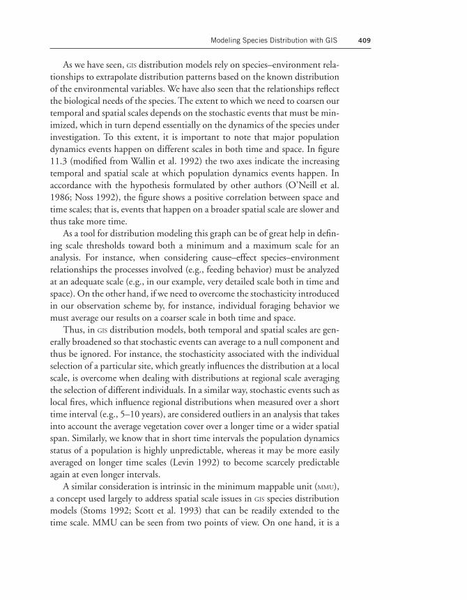
Modeling Species Distribution with GIS 409
As we have seen, GIS distribution models rely on species–environment rela-tionships to extrapolate distribution patterns based on the known distributionof the environmental variables. We have also seen that the relationships reflectthe biological needs of the species. The extent to which we need to coarsen ourtemporal and spatial scales depends on the stochastic events that must be min-imized, which in turn depend essentially on the dynamics of the species underinvestigation. To this extent, it is important to note that major populationdynamics events happen on different scales in both time and space. In figure11.3 (modified from Wallin et al. 1992) the two axes indicate the increasingtemporal and spatial scale at which population dynamics events happen. Inaccordance with the hypothesis formulated by other authors (O’Neill et al.1986; Noss 1992), the figure shows a positive correlation between space andtime scales; that is, events that happen on a broader spatial scale are slower andthus take more time.
As a tool for distribution modeling this graph can be of great help in defin-ing scale thresholds toward both a minimum and a maximum scale for ananalysis. For instance, when considering cause–effect species–environmentrelationships the processes involved (e.g., feeding behavior) must be analyzedat an adequate scale (e.g., in our example, very detailed scale both in time andspace). On the other hand, if we need to overcome the stochasticity introducedin our observation scheme by, for instance, individual foraging behavior wemust average our results on a coarser scale in both time and space.
Thus, in GIS distribution models, both temporal and spatial scales are gen-erally broadened so that stochastic events can average to a null component andthus be ignored. For instance, the stochasticity associated with the individualselection of a particular site, which greatly influences the distribution at a localscale, is overcome when dealing with distributions at regional scale averagingthe selection of different individuals. In a similar way, stochastic events such aslocal fires, which influence regional distributions when measured over a shorttime interval (e.g., 5–10 years), are considered outliers in an analysis that takesinto account the average vegetation cover over a longer time or a wider spatialspan. Similarly, we know that in short time intervals the population dynamicsstatus of a population is highly unpredictable, whereas it may be more easilyaveraged on longer time scales (Levin 1992) to become scarcely predictableagain at even longer intervals.
A similar consideration is intrinsic in the minimum mappable unit (MMU),a concept used largely to address spatial scale issues in GIS species distributionmodels (Stoms 1992; Scott et al. 1993) that can be readily extended to thetime scale. MMU can be seen from two points of view. On one hand, it is a

410 CORS I , D E LEEUW, AND SK IDMORE
Figure 11.3 Population dynamics event in relation to time and space scales (modified from Wallinet al. 1992).
property of the data set that is being analyzed, that is, the minimum dimen-sion of an element (e.g., a polygon representing vegetation types of a given cat-egory, the time span between successive manifestations of a given ecologicalevent) that can be displayed and analyzed. On the other, it indicates the kindof averaging that must be carried out to smooth noise introduced by stochas-ticity. In fact, in the case of local fires, if the MMU is defined as larger than theextent of the fire in both time and space, the fire is automatically excludedfrom the analysis.
When dealing with scales on a practical basis, it should be noted that thestructural complexity of distribution modeling can be simplified according tothe hierarchical hypothesis (O’Neill et al. 1986) that states that at any givenscale particular environmental variables drive the ecological processes. Thusweather becomes important at very broad spatial scales (e.g., continentalscale). This is the basis of approaches behind models such as BIOCLIM (Busby1991), that of Walker (1990), and that of Skidmore et al. (1996); all of themdescribe species distribution at a continental scale in terms of their direct rela-tionship to climatic data. At successively finer scales such as regional land-scapes, land form and topography play an important part (Haworth and

Modeling Species Distribution with GIS 411
Thompson 1990; Aspinall 1992; Flather et al. 1992; Aspinall and Veitch1993), whereas at the most local scales, indigenous land use structures becomeincreasingly significant (Thomasma et al. 1991; Picozzi et al. 1992; Herr andQueen 1993) to the extent that even an individual stand of timber (Pausas etal. 1995) or a single pond (Genard and Lescourret 1992) can play a role. Gen-erally speaking, the factors that are important vary according to scale, meaningthat factors that are important at one scale level can lose their importance(Noss 1992), or at least much of it, at others.
As with any type of classification, the relationship between scale and envi-ronmental variables that drive ecological processes should not be taken toorigidly, and although most authors tend to agree that for broader scales climateis the most important factor, the same cannot be said when trying to identifythe driving forces at finer scales. For instance, variables considered useful atcoarser scales are used in detailed studies, as in the cases of Pereira and Itami(1991) and Ross et al. (1993), which use topography to explain species distri-bution at a much finer scale than the regional one. The same considerationapplies to the studies of Aspinall and Matthews (1994), which use climaticdata on a regional scale. On the other hand, land use is often used in distribu-tion models developed at regional scale (Livingston et al. 1990; Flather andKing 1992).
Finally, we must consider that distribution is the result of the interaction ofmany different biological events and that an ecological event cannot bedescribed exhaustively on any single specific scale, but is the result of complexinteractions of phenomena happening at different scales (Levin 1992; Noss1992). Thus the limit of the applicability of a given environmental variable todescribe distribution on any given scale may not be so sharp and the challengeis toward the integration of different scales in the description of the species’distributions. Buckland and Elston (1993) gave an example of the integrationof environmental variables stored at different resolutions within the same dis-tribution model.
It is important to note that the concept of scale not only determines thebiological extent to which a distribution model can be applied but also affectsthe use that can be made of such a model for conservation. Also, conservationactions can be seen as having a hierarchical approach (Kolasa 1989). Forinstance, Scott et al. (1987) identified six different levels of intervention: land-scape, ecosystem, community, species, population, and individual. Not sur-prisingly, conservation actions tend to become more effective and less expen-sive when the assessment moves toward broader scales, that is, when one movesfrom the individual to the landscape approach (Scott et al. 1987). Obviously

412 CORS I , D E LEEUW, AND SK IDMORE
this relates only to the extent of the analysis, not to its resolution. Nevertheless,on a cost–benefit basis, it is generally more efficient to address conservation-related issues at a coarser scale, which enables a landscape approach, than toconcentrate on a more detailed scale (e.g., individual or population level),which requires high-resolution data to be analyzed that are either too preciseor simply too abundant in terms of storage requirements to be analyzed prof-itably with a landscape approach.
What economics suggests is that conservation science needs to have abroader view of phenomena. A broad-scale approach and the possibility of pre-dicting the potential dynamics of spatial patterns are needed to manage frag-mentation of suitable environments and the inevitable metapopulation struc-ture of the resulting population (Noss 1992). May (1994) indicates that whenmultiple levels of biological organization are concerned, as in a typical conser-vation action, the best management approach can be achieved on the regionallandscape scale (103 to 105 km2). This scale level has suffered historically fromlimitations in the tools available for consistent analysis and is the one that hasgained the most from the evolution of GIS; in fact, most of the distributionmodels based on GIS address problems at regional landscape level.
DATA AVAILABILITY
Data availability and quality are two of the three limiting factors in the devel-opment of GIS-based species distribution models (the other being reliability ofthe models themselves [Stoms et al. 1992], which is discussed later in this chap-ter). The problem of developing extensive data sets of environmental variablesis limited by economic and political rather than technical constraints. Estes and Mooneyhan (1994) list a number of different attitudes of governmentsthroughout the world that limit the availability of high-resolution, “science-quality”5 environmental data sets. These range from military classification ofthe data, thereby precluding the use of the data to the scientific community, tothe low political priority that certain governments give to environmental issues.Moreover, even when policy is not an obstacle to the production and availabil-ity of data sets, entire nationwide data sets are sometimes lost during revolu-tions, wars, and civil disturbances. To this it should be added that some gov-ernments (e.g., the European Union countries) ask high prices for data sets,which are generally acquired with tax money, actually preventing their broaduse in any type of activity and more specifically in environmental research.
In many cases, high-quality site-specific data sets are generated for a partic-ular research project but are compiled with nonstandard techniques, rendering

Modeling Species Distribution with GIS 413
them unsuitable for combination and the achievement of more extensiveknowledge of an area.
In the past few years there has been an increasing effort to develop meta-databases of available data sets throughout the world, and the problem is beingaddressed by national and international organizations (e.g., United NationsEnvironmental Programme, World Bank, U.S. Geological Survey [USGS],European Environmental Agency). These initiatives still do not address theproblem of producing high-quality data sets, but at least they are a start in col-lating existing data sets. An important example is given by the joint efforts ofthe USGS, the University of Nebraska–Lincoln, and the European Commis-sion’s Directorate General Joint Research Centre, which are generating a 1-km-resolution Global Land Cover Characterisation (GLCC) database suitablefor use in a wide range of environmental research and modeling applicationsfrom regional up to continental scale. All data used or generated during thecourse of the project (source, interpretations, attributes, and derived data),unless protected by copyrights or trade secret agreements, are distributedthrough the Internet. This effort goes in the direction of producing and dis-tributing homogeneous medium-resolution high-quality data sets with knownstandards of accuracy.
Further aspects of raw data sets are discussed in the next section, where thequality of the data used to build models is discussed. We do not discuss thisissue further here because we do not believe it to be a problem that can beaddressed directly by conservation biologists or ecologists, although they cancontribute to developing awareness of the need for standardization of data setsand for their production and dissemination.
VALIDATION AND ACCURACY ASSESSMENT
Generally, the main function of a GIS-based species distribution model is toproduce a map or its digital analogue for assessment of management and con-servation actions. Possibly the most important question to be asked by a useris ‘how accurate is the distribution map that has been produced?’
Many articles have been written on the sources of error in the data layersthat may be included in a GIS. Nevertheless, few authors of papers dealing withanimal distribution include an assessment of the accuracy of their model anda validation of the product. Because we believe this issue to be central to theentire process of species distribution modeling, the aim of this section is toreview sources of error in GISs, to discuss methods of assessing mapping accu-racy, and to evaluate the accumulation of thematic map errors in GISs, thus pro-

414 CORS I , D E LEEUW, AND SK IDMORE
viding a framework for assessment of the accuracy of distribution modelsdeveloped with GIS.
Source of errors
GIS data layers are traditionally classified according to their data structure,either raster or vector. To a certain extent, both error sources and accuracy eval-uation methods have been investigated following this traditional classification.
Raster images may be obtained from remote sensing instruments carried byaircraft or spacecraft platforms, or by converting an existing line map (vectordata structure) to a raster data structure. Two types of error are inherent inremotely sensed images: geometric and radiometric. These error sources areaddressed in detail in numerous monographs and papers, including Colwell(1983) and Richards (1986).
A raster image is usually made up of a regular grid of adjacent rectangularcells or pixels (i.e., a rectangular tessellation). Geometric error in a remotelysensed image is caused by movement in the remote sensing platform; distor-tion caused by the earth’s curvature and terrain; different centrifugal forcesfrom earth affecting spacecraft movement; the earth’s rotational skew; distor-tions introduced by the remote sensing device itself, including systematic dis-tortions caused by sampling sequentially from each detector and nonlinearscanning (Adomeit et al. 1981); and errors introduced by the georeferencingprocess. Geometric error causes a point on the remotely sensed image to occurin the wrong position relative to other points in the image.
Correction of geometric errors in remotely sensed data is now a routineaspect of their preprocessing. The map or image is usually rubber-sheeted to fitit to an appropriate map projection. Corrected images with geometric errors ofless than 0.5 pixel are now obtainable and acceptable6 (Ford and Zanelli 1985;Ehlers and Welch 1987; Skidmore 1989b). However, the base maps fromwhich control point information is derived may be of poor quality. Bell (1986)reported that maps used to geometrically correct images of the Great BarrierReef contained errors of up to 1 km. The accurate selection of control pointsis crucial in obtaining acceptable results.
Points within a rubber-sheeted image are no longer on a regular gridbecause they have been warped to fit into the projection defined by the groundcontrol points (GCPs). To obtain a regular grid, an interpolation method is usedto nominate a value for a regular grid point that falls between the points in therubber-sheeted image. Lam (1983) provides an excellent review of other inter-polation methods, including splines, finite difference, and kriging.
Radiometric errors occur as a result of differential scattering of electromag-

Modeling Species Distribution with GIS 415
netic radiation at varying wavelengths, sensors that have poorly calibratedmultiple detectors within a band, sensor calibration error, signal digitizationerror, and scene-specific error such as off-nadir viewing, irradiance variation,and terrain topography (Richards 1986). Correction of band-to-band distor-tion is performed using image histograms (shifted to the origin to removeatmospheric scattering effects), whereas line striping effects are reduced by cal-ibration of detectors or by matching detector statistics during computer pro-cessing (Teillet 1986).
A final type of error may be caused by a time lag between ground truthingand image collection. In this case, pixels may be noted as incorrect in the errormatrix (described later in this chapter) when they may be actually correct atthe time of image acquisition.
Vector images have been traditionally recorded and stored as maps. Mapsare subject to many errors. Some errors are introduced during the creation ofthe map, such as the original line smoothing, which may not follow the trueisolines on the ground (Chrisman 1987). Other errors may be associated withthe physical medium used to store the map (e.g., paper stretch and distortion).
Maps may be represented in computer GISs by a variation of the vector datastructure (Peuquet 1984) or converted to a raster data structure. In its simplestform, the vector data structure has map lines approximated to a set of points(nodes), which are linked by lines (or arcs). Vector data may be obtained bydigitization.
Digitization introduces a number of errors. Varying line thickness on theoriginal map requires automatically scanned vector lines to be thinned. Dur-ing manual digitization the center of the map line must be followed carefullyif the map lines vary in thickness (Peuquet and Boyle 1984). This requires verycareful hand digitizing or high-accuracy automatic scanners. The number ofvertices (points) used to approximate a curve is also critical (Aldred 1972). Toofew vertices will result in the line appearing stepped, and too many vertices cre-ate large data volumes. Thus, even with extreme care, error is introduced dur-ing digitization.
As for raster images, the main method of correcting geometric error in vec-tor images is by using ground control points from a cartographically correctmap to transform the vector image to a known projection.
Data layer error quantification
Methods for quantifying error in a raster data layer are based on the errormatrix (also called a contingency table or confusion matrix) concept, firstexpounded for remotely sensed data in the 1970s (Hoffer 1975).

416 CORS I , D E LEEUW, AND SK IDMORE
The aim of the error matrix is to estimate the mapping accuracy (i.e., theproportion of correctly mapped pixels) within an image. An error matrix isconstructed from points sampled from the image. The reference (or verifica-tion) data are normally represented along the columns of the matrix, and arecompared with the classified (or image) data represented along the rows. Themajor diagonal of the matrix represents the agreement between the two datasets (table 11.3).
To check every cell for correctness would be impossible except in the small-est map area, so various sampling schemes have been proposed to select pixelsto test. The design of the sampling strategy, the number of samples required,and the area of the samples have been debated by the remote sensing and GIS
community.As with any sampling problem, one is obviously trying to select the sam-
pling design that gives the smallest variance and highest precision for a givencost (Cochran 1977). A number of alternative designs have been proposed forsampling the pixels to be used in constructing the error matrix. Berry andBaker (1968) recommended the use of a stratified systematic sample.7 Theadvantage of systematic sampling over random sampling is that sample unitsare distributed equitably over the area. The disadvantage is that the resultingsample is weighted in favor of the class covering the largest area and that classeswith a small area may not be sampled at all.
Simple random sampling in land evaluation surveys emphasizes larger areasand undersamples smaller areas (Zonneveld 1974). Zonneveld (1974) sug-gested that a stratified random sample was preferable, and Van Genderen et al.(1978:1135) agreed that a stratified random sample is “the most appropriatemethod of sampling in resource studies using remotely sensed data.”
Rosenfield et al. (1982; see Berry and Baker 1968) suggested a stratifiedsystematic unaligned sampling procedure (i.e., an area weighted procedure) asa first-stage sample to assist in identifying categories occupying a small area,followed by further stratified random sampling for classes with fewer than thedesired minimum number of points. Todd et al. (1980) argued that single-stage cluster sampling is the cheapest sampling method because multipleobservations can be checked at each sample unit on the ground.
Congalton (1988) simulated five sampling strategies (simple random sam-pling, stratified random sampling, cluster sampling, systematic sampling, andstratified systematic unaligned sampling) using a different number of samplesover remotely sensed images of forest, rangeland, and grassland. The aim of thestudy was to ascertain the effect of different sampling schemes on estimatingmap accuracies using error matrices. He concluded that great care should be

Modeling Species Distribution with GIS 417
Table 11.3 Typical Error Matrix
Classification of Pixels (ground truth)
Class I II III VI V VI VII VIII IX Total
Classification I 14 3 7 2 5 7 38of pixels IV 4 8 3 2 1 3 21(model) V 2 16 1 19
VI 1 1 2VII 1 3 3 7VIII 2 2IX
Total no. of pixels 20 19 38 6 17 8 8 17 2 135Overall classification accuracy 50.4%.a
Example drawn from the classification of vegetation types from a satellite image. I = yertchuk, II =gum/stringybark, III = silvertop ash, IV = blue-leaf stringybark, V = clearcut/road, VI = tea tree, VII =gum/silvertop ash, VIII = black oak, IX = unclassified.aRatio of the sum of correctly classified pixels in all classes to the total number of pixels tested.
taken in using systematic sampling and stratified systematic unaligned sam-pling because these methods could overestimate population parameters. Con-galton (1988) also stated that cluster sampling may be used, provided a smallnumber of pixels per cluster are selected (he suggested a maximum of 10 sam-ple pixels per cluster). Stratified random sampling worked well and may beused where small but important areas must be included in the sample. How-ever, simple random sampling may be used in all situations.
The number of samples may be related to two factors in map accuracyassessment: the number of samples that must be taken in order to reject a mapas being inaccurate and the number of samples required to determine the trueaccuracy within some error bounds for a map.
Van Genderen et al. (1978) pointed out that we want to know, for a givennumber of sample pixels, the probability of accepting an incorrect map. Inother words, when high mapping accuracy is obtained with a small sample(e.g., 10 items), there is a chance that no pixels that are in error may be sam-pled (i.e., a type II error8 is committed). The corollary, as stated by Ginevan(1979), is also important: The probability of rejecting a correct map (i.e., com-mitting a type I error) must also be determined.

418 CORS I , D E LEEUW, AND SK IDMORE
Van Genderen and Lock (1977) and Van Genderen et al. (1978) arguedthat only maps with 95 percent confidence intervals (i.e., b = 0.05) should beaccepted and proposed a sample size of 30. Ginevan (1979) pointed out thatVan Genderen et al. (1978) made no allowance for incorrectly rejecting anaccurate map. The tradeoff one makes using Ginevan’s more conservativeapproach is to take a larger sample, but in so doing reduce the chance of reject-ing an acceptable map. Hay (1979)9 concluded that minimum sample sizeshould be 50, greater than that of Van Genderen and Lock (1977).
The number of samples must be traded off against the area covered by asample unit, given a certain quantity of money to perform a sampling opera-tion. Curran and Williamson (1986) asked whether many small-area samplesor a few large-area samples should be taken. The answer is that it depends onthe cover type being mapped; a highly variable cover type such as rainforest isbetter suited to many small-area samples, whereas for more homogeneouscover types it is more efficient to take fewer large-area samples.
Generally, mapping of heterogeneous classes such as forest and residentialland is more accurate at 80-m resolution than at finer resolutions such as 30 m(Toll 1984); however, more homogeneous classes such as agricultural land andrangeland are more accurately mapped at 30 m than at 80 m (Toll 1984). Thereason for this is the tradeoff between ground element size and image pixel res-olution.
Based on the error matrix, different measures of accuracy can be derived. Acommonly cited measure of mapping accuracy is the overall accuracy, which isthe number of correctly classified pixels (i.e., the sum of the major diagonalcells in the error matrix) divided by the total number of pixels checked (table11.3). Anderson et al. (1976) suggested that the minimum level of interpreta-tion accuracy in the identification of land use and land cover categories shouldbe 85 percent.
Overall classification accuracy is the ratio of the total number of correctlyclassified pixels to the total number of pixels in each class (Kalensky andScherk 1975).
Cohen (1960) and Bishop et al. (1975) defined a measure of overall agree-ment between image data and the reference (ground truth) data called Kappaor K. K ranges in value from 0 (no association, that is, any agreement betweenthe two images equals chance agreement) through 1 (full association, or per-fect agreement between the two images). K can also be negative, which signi-fies a less than chance agreement.
The methods just discussed for quantifying error in raster images areequally applicable to quantifying error in vector polygons. Instead of checking

Modeling Species Distribution with GIS 419
whether an image pixel is correctly classified, a point within the polygon is ver-ified against the ground truth information. A specific problem encounteredwith vector images is ground truth samples that occur across boundary lines;in this case the class with the largest area within the sample area may beselected to represent the vector map image.
A method of assessing map accuracy based on line intersect sampling wasdescribed by Skidmore and Turner (1992). Line intersect sampling is used toestimate the length of cover class boundaries on a map10 that coincide with thetrue boundaries of the cover classes on the ground. A ratio of coincidentboundary to total boundary is proposed as a measure of map accuracy and thisratio is called the boundary error. Although this technique was developed forvector maps, it is equally applicable to raster maps.
Skidmore and Turner (1992) found that the true boundary lengths werenot significantly different from the estimated boundary lengths sampled usingline intersect sampling, with a ′ = 0.05. The estimated boundary accuracy (64percent) was extremely close to the true boundary accuracy (65.1 percent), andthere was no significant difference between the true and estimated boundaryaccuracy.
Reliability of the output
Apart from assessing the accuracy of the original data sets used to produce GIS
models, the final products of the modeling effort must be validated.As previously evidenced, the process of model building takes its move from
a number of data maps of the same region (e.g. elevation, soils, ground cover),which are digitized and geographically rectified to a common projection in aGIS. Such maps may be stored as a series of layers in a GIS. Each point within apolygon, or each cell in a raster layer (where each raster cell is assigned onevalue), takes the values of the layers directly above the point. The model is thenbuilt defining specific questions that may be asked about specific points orcells, such as the slope or aspect at the point. Eventually the biologist is inter-ested in mapping areas that satisfy the known ecological requirements of aspecies (e.g., slope greater than 30°, with erodible soils, occurring on asoutherly aspect). By overlaying the map layers, such simple queries may beanswered.
Nevertheless, the simple process of overlaying layers propagates the errorsof the original data and sometimes amplifies them. If the sources of errors areidentified and their accuracy is known, an estimate of the accuracy of the finaloutput can be achieved through error propagation analysis.

420 CORS I , D E LEEUW, AND SK IDMORE
Sources of errors range from those evidenced in the previous paragraphs tothose inherent to nonspatial or text data that are also part of a GIS model. Forinstance, nonspatial data include knowledge or rules used by expert systems(Skidmore 1989b). All these errors contribute to error accumulation whenoverlaying GIS data layers.
Composite overlaying is the simplest overlaying technique. Two or morelayers are combined, and the raster locations (or polygons formed) describe theunion of the classes on the layers. The composite overlay is in effect a univer-sal Boolean and operation over the whole map. That is, for a two-layer data setcomprising layer X and layer Y, we note Xi=1,n > Yj=1,m (i.e., the intersection ofX and Y for the n classes in map X and the m classes in map Y) at all points overthe map.
Arithmetic and mathematical operators that may be applied to two ormore layers include addition, subtraction, multiplication, division, maximum,minimum, average, and exponent.
The method by which error is accumulated during the overlaying processis important for modeling error in the final map products. The first necessityfor modeling map error accumulation is to quantify the error in the individuallayers being overlaid. As discussed earlier, a lot of work has been done on thisproblem, with some tangible results.
Newcomer and Szajgin (1984) used probability theory to calculate erroraccumulation through two map layers. They assumed that the two map layerswere dependent; that is, if we select a cell that is in error in layer 1 then that actreduces the probability of selecting an erroneous cell from layer 2. If the datalayers are independent, then an erroneous cell selected from layer 1 does notreduce the probability of selecting an incorrect cell from layer 2.
Using the statistics of Parratt (1961) with empirical data, Burrough (1986)concluded that with two layers of continuous data, the addition operation isunimportant in terms of error accumulation. The amount of error accumu-lated by the division and multiplication operations is much larger. The largesterror accumulation occurs during subtraction operations. Correlated variablesmay have higher error accumulation rates than noncorrelated data becauseerroneous regions tend to coincide and concentrate error rates there.
The use of Bayesian logic for GIS overlaying is explained in Skidmore(1989b). As with Boolean, arithmetic, and composite overlaying, there isinherent error in the individual data layers when overlaying using Bayesianlogic. In addition, Bayesian overlaying uses rules to link the evidence to thehypotheses; the rules have an associated uncertainty and are an additionalsource of error.

Modeling Species Distribution with GIS 421
A number of possible solutions are suggested for modeling accumulation oferror in a GIS. These include reliability diagrams and a probabilistic approach.
Wright (1942) suggested that reliability diagrams should accompany allmaps. He also emphasized that the sources used to generate different regionsof the map have varying accuracy and these sources should be stated clearly onthe map. For example, one region may have been mapped using low-altitudeaerial photography and controlled ground survey, and would therefore bemore accurate than another region mapped using high-altitude photographyand only reconnaissance survey. This theme was taken up by Chrisman (1987)and MacEachren (1985), who suggested that such a reliability diagram show-ing map pedigree should be included as an additional layer accompanyingeach map layer in a GIS. However, for the purposes of error accumulation mod-eling, reliability diagrams do not provide a quantitative statement about theaccuracy (or error) of the map.
The supervised nonparametric classifier described by Skidmore and Turner(1988) and Skidmore et al. (1996) classified remotely sensed and GIS digitaldata. The classifier gives for all cells the empirical probability of correct classi-fication for each class according to the training area data and thereby gives anindication of map accuracy.
The few methods proposed for modeling error accumulation are limited intheir application. Working with ideal data, these methods do allow some con-clusions to be drawn about error accumulation during GIS overlay operations.However, the methods break down when used with map layers created underdifferent conditions than assumed by the methods.
Newcomer and Sjazgin (1984) used probability theory to model erroraccumulation, whereas Heuvelink and Burrough (1993) modeled the accu-mulation of error in Boolean models, using surfaces interpolated by kriging asthe estimated error source.
Sensitivity analysis
When no information is available on the extent of the errors of the originaldata sets or on the type of error propagation function applicable to the model,a way of defining levels of reliability of the output is to analyze its variabilitysubject to changes in the input parameters. In the this chapter we have seenpossible sources of variability and uncertainties that can arise in the deductiveand inductive approaches in species distribution modeling. They range fromsubjective errors introduced by the specialist who defines the species–environ-ment relationship to locational errors of species observation caused by possible

422 CORS I , D E LEEUW, AND SK IDMORE
biases in the sampling scheme or inaccuracy of the instrument used to locatethe species (e.g., radiotelemetry, global positioning system). A through discus-sion of the sources of uncertainties in species distribution modeling can befound in Stoms et al. (1992).
Once the sources and ranges of variability are identified, different input datasets can be systematically produced, selecting the variates (sensu Sokal andRohlf 1995) from the variability range of the original input variables. Thesealternative data sets are used to build alternative models that can be comparedwith the original one, identifying the variability induced in the output by theuncertainty of the input variables. The variability induced in the output is ameasure of the overall performance of the model and can be compared with apredetermined acceptable significance level. As a general rule, when dealingwith great uncertainties in the measures of the input variables, a greater inertia(less subject to changes in the results) of the model is generally preferable.
Sensitivity analysis does not replace validation but can be used at any stageof the model-building process to identify the parameters that should be mon-itored more carefully to maximize the reliability and the accuracy of theresults.
j Discussion
The use of GIS in species distribution modeling should follow precise steps in which each of the issues discussed in this chapter is accounted for. First of all, we recommend more unambiguous use of some key terms such as scaleand habitat. The latter seems to be a particular problem not limited to GIS
applications but spanning the entire field of ecological studies (Hall et al.1997). We believe that GIS can be a valid tool to overcome the current ambi-guity between the species-related and land-related concepts of the term habi-tat. As a matter of fact, the latter was introduced as a way of dealing with prob-lems related to environmental mapping using traditional tools, and theenhancements introduced by GIS do overcome those problems. In the mean-time, however, we suggest replacing the word habitat with more unproblem-atic terms such as environment.
The ambiguity of the term habitat and most of the works on habitat useand habitat selection have also given rise to the question of whether GIS-basedmodels can be used to explain the causal event of a species–environment rela-tionship. In our opinion, use of GIS is not central to a better understanding ofcausal effects in a species–environment relationship, especially if the quality of

Modeling Species Distribution with GIS 423
data does not support both high-resolution and large-extension analyses. Cur-rently our analytical capabilities are limited by the lack of high-resolution,global coverage data sets. Nevertheless, the use of GIS’s spatial analysis tools inthe framework of a controlled environment in which all the key variables aremonitored at an adequate resolution can increase our ability to assess causaleffects in species–environment relationships.
Apart from further generic considerations, we think that a few importantissues have been overlooked in these first years of application of GIS to the fieldof ecological modeling and especially in the field of species distribution mod-eling. There has been inadequate discussion and consideration of the assump-tions underlying the model-building process and the related issues of spatialand temporal scale, which are of paramount importance for sound scientific11
use of GIS. Adequately discussed assumptions can justify the development of amodel. Whenever a hypothesis is stated and a model is built to test its congru-ence, it should be regarded as a problem-solving tool. For instance, we willnever really know what will be the outcome of alternative managementoptions, but we can state different hypotheses, state the assumptions that mustbe met to make each hypothesis hold true, and try to model the result of thedifferent options. In such cases we don’t have direct control over the results ofthe management action; we can only ensure that the assumptions are met. Thismeans that the output of the model will hold true if the assumptions are metand if the model is built on the logical consequences of these assumptions. Insuch cases validation, meant as an independent estimate of the truth, can to acertain extent be neglected (Starfield 1997). Nevertheless, most of the timeassumptions are not adequately discussed and this is particularly evident whendealing with the constraints of scale dependency of biological events. Probablythe issues of scale still suffer from inadequate support from the available tools.For instance, we still lack convenient ways of handling spatiotemporal data inGIS software packages, not to speak of analyzing the two components together.
If validation can be neglected somewhat when dealing with hypothesis-testing models, it becomes a fundamental issue when building analytical mod-els, which are built to assess species–environment relationships and ecologicalprocesses. In such cases, validation steps must be included from the beginningof the model building process, first assessing the quality and reliability of theraw data used, then evaluating the limits of the relationships that drive theprocess and finally analyzing the correspondence of the output with the truth.
Validation can be a costly exercise in model building, and efforts are beingmade to find a cost-effective approach to this issue. Because the issue of vali-dation is general to GIS modeling and especially GIS ecological applications, it

424 CORS I , D E LEEUW, AND SK IDMORE
can benefit from the experience derived from other fields of science (e.g., RS).Methods for summarizing the accuracy of raster and vector maps using pointsamples and error matrices are now widely used in GIS and are beginning tofind their way into ecological applications as well. However, standard tech-niques have not had universal acceptance for a number of reasons. For exam-ple, a number of alternative sampling designs have been proposed for analyz-ing the accuracy of imagery. The choice of sampling design is often subject tothe particular problems associated with the area to be ground-truthed. How-ever, a number of general trends are obvious from the GIS and RS literature.Random and stratified random sampling are acknowledged to maximize pre-cision and accuracy (though at a higher cost than cluster sampling or system-atic sampling). It should be noted that in highly heterogeneous landscapes(e.g., native forests, especially tropical forests), stratification is often too costlyto consider. Cluster sampling offers reduced sampling costs, but in order to beeffective it depends on low intracluster variance. Systematic sampling schemesmay lead to a bias in parameter estimation if periodic errors align with thesampling frame (e.g., as a result of image banding or linear topographic fea-tures, as in the Allegheny Mountains of Pennsylvania).
GIS data layers contain numerous errors. These pose a number of problemsas errors accumulate during the process of analysis and model building.Although modeling the accumulation of error during GIS overlay analysis is stillin its infancy, some methods for measuring error accumulation during GIS
analysis have been discussed.Any procedure to reduce mapping error in individual layers in a GIS will
improve the mapping accuracy of an overlay generated from the GIS. Until bet-ter error-modeling techniques are developed for GISs, descriptive statisticsshould ideally be calculated for each layer in a GIS, as well as for each layer pro-duced by GIS modeling. The descriptive statistics should include overall map-ping accuracies as well as class mapping accuracies. An alternative way of defin-ing the performance of a GIS model, thus assigning a level of reliability to itsresults, is sensitivity analysis that identifies crucial parameters. These parame-ters are those that, within their range of variation, determine the highest vari-ation in the model output.
j Conclusions
A common opinion among epistemologists is that we are facing a breakbetween the development of advanced technologies and our needs and abilities

Modeling Species Distribution with GIS 425
to use them. As a result of this break, sophisticated systems are often used forsimple operations and their use becomes a goal in itself. Toraldo di Francia(1978) names this paradox “the law of inversion between the goal and theinstrument.” This has also been the case with gis: the emphasis was on the useof the tool rather than on solving the problems to which it was applied. Dur-ing the infancy of the tool’s development its enthusiastic and acritical applica-tion was a clear evidence of the low awareness of the tool’s limitations.Although we don’t believe that the infancy of GIS is over, in recent years we haveseen a growth in the capabilities of the tool and the awareness of its users. Wethink that we have enough case studies to define a logical framework in whichthe process of gis modeling and more specifically species distribution model-ing should be kept. We have tried to accomplish this by identifying the issuesthat must be addressed during the entire process.
In an era in which the need to acquire and analyze data at wider scales isincreasing and globalization in environmental assessment applications isbecoming urgent, we should not waste the opportunity GIS offers to wildlifebiologists to cope with these needs. This does not mean that GIS modeling cansubstitute for fieldwork and direct observation; especially in the case of rare orendangered species, all management action should be based on direct site-spe-cific studies. Nevertheless, sound GIS distribution models, which can beachieved by addressing the different issues we have tried to address in thischapter, can help to identify areas that require more detailed investigation.
Acknowledgments
We thank Luigi Boitani and Todd Fuller for giving us the opportunity toorganize these ideas. The chapter is also the result of suggestions and com-ments from Luigi Boitani, Alessandra Pellegrini, Iacopo Sinibaldi, and twoanonymous reviewers.
Notes
1. Area of occupancy is defined as the area within the species’ extent of occurrence that isoccupied by a taxon, excluding cases of vagrancy. The measure reflects the fact that a taxonwill not usually occur throughout the area of its extent of occurrence, which may containunsuitable habitats, for example. The area of occupancy is the smallest area essential at anystage to the survival of existing populations of a taxon (e.g., colonial nesting sites, feedingsites for migratory taxa) (IUCN1995).
2. Bibliographic database of literature in earth sciences, ecology, and geography pub-lished by Elsevier.

426 CORS I , D E LEEUW, AND SK IDMORE
3. Habitat is also used in connection to humankind. In this chapter the term habitatrefers to plant and animal species excluding human beings.
4. Here habitat relates to species, whereas it refers to land in the next sentence.5. “‘Science-quality’ means that, in so far as both practical and possible, the errors
inherent in the overall production of [these] maps have been documented” (Estes andMooneyhan 1994).
6. Note that the accuracy of the geometric correction is sometimes expressed as rootmean square (RMS) error, which is the standard error (of the difference between the trans-formed GCPs and the original GCPs) multiplied by the pixel size.
7. Each stratum has an unaligned systematic sample.8. Type I errors have been called “consumer’s risk” and type II errors “producer’s risk” by
Fung and LeDrew (1988) and others. These terms are taken from a branch of statisticscalled acceptance sampling. For the sake of consistency and in order to use conventional sta-tistical terms, type I and type II errors are used here.
9. Hay (1979) noted that he developed the ideas expounded by Van Genderen andLock (1977).
10. The map may be generated from remotely sensed imagery or by traditional carto-graphic methods such as aerial photograph interpretation.
11. Here scientific is used in the sense of scientific method: the recognition and formu-lation of a problem, the collection of data through observation and experiment, and the for-mulation and testing of the hypotheses.
Literature Cited
Adomeit, E. M., D. L. B. Jupp, C. I. Margules, and K. K. Mayo. 1981. The separation oftraditionally mapped land cover classes by Landsat data. In A. N. Gillison and D. J.Anderson, eds., Vegetation classification in Australia, 150–165. Canberra, Australia: ANU
Press.Agee J. K., S. C. F. Stitt, M. Nyquist, and R. Root. 1989. A geographic analysis of histori-
cal grizzly bear sightings in the North Cascades. Photographic Engineering and RemoteSensing 55: 1637–1642.
Akçakaya, H. R. 1993. RAMAS/GIS: Linking landscape data with population viability analysis.New York: Applied Biomathematics.
Akçakaya, H. R., M. A. McCarthy, and J. L. Pearce. 1995. Linking landscape data withpopulation viability analysis: Management options for the helmeted honeyeaterLichenostomus melanops cassidix. Biological Conservation 73: 169–176.
Aldred, B. K. 1972. Point-in-polygon algorithms. Peterlee, U.K.: IBM.Allen, A. W., P. A. Jordan, and J. W. Terrell. 1987. Habitat suitability index models: Moose,
Lake Superior region. U.S. Fish and Wildlife Service Biological Report 82.Anderson, J. R., E. E. Hardy, J. T. Roach, and R. E. Witmer. 1976. A land use and land cover
classification system for use with remote sensor data. Washington, D.C.: U.S. GeologicalSurvey.
Aspinall, R. 1992. An inductive modeling procedure based on Bayes’ theorem for analysis

Modeling Species Distribution with GIS 427
of pattern in spatial data. International Journal of Geographic Information Systems 6:105–121.
Aspinall, R. and K. Matthews. 1994. Climate change impact on distribution and abun-dance of wildlife species: An analytical approach using GIS. Environmental Pollution 86:217–223.
Aspinall, R. A. and N. Veitch. 1993. Habitat mapping from satellite imagery and wildlifesurvey data using a Bayesian modelling procedure in a GIS. Photographic Engineering andRemote Sensing 59(4): 537–543.
Atkinson, S. F. 1985. Habitat based methods for biological impact assessment. Environ-mental Professional 7: 265–282.
Bailey, R. G. 1988. Problems with using overlay mapping for planning and their implica-tions for geographic information systems. Environmental Management 12(1): 11–17.
Begon, M., J. L. Harper, and C. R. Townsend. 1990. Ecology: individuals, populations andcommunities. Cambridge, U.K.: Blackwell.
Bell, A. 1986. Satellite mapping of the Great Barrier Reef. Ecos 47:12–15.Berry, B. J. L. and A. M. Baker. 1968. Geographic sampling. In B. J. L. Berry and D. F.
Marble, eds., Spatial analysis: A reader in statistical geography, 230–248. EnglewoodCliffs, N.J.: Prentice Hall.
Bishop, Y. M., S. E. Fienburg, and P. W. Holland. 1975. Discrete multivariate analysis: The-ory and practice. Cambridge, Mass.: MIT Press.
Bozek, M. A. and F. J. Rahel. 1992. Generality of microhabitat suitability models for youngColorado River trout (Oncorhynchus clarki pleuriticus) across site and among years inWyoming streams. Canadian Journal of Aquatic Science 49: 552–564.
Breininger, D. R., M. J. Provancha, and R. B. Smith. 1991. Mapping Florida scrub jayhabitat for purposes of land-use management. Photographic Engineering and RemoteSensing 57: 1467–1474.
Buckland, S. T. and D. A. Elston. 1993. Empirical models for the spatial distribution ofwildlife. Journal of Applied Ecology 30: 478–495.
Bunnell, F. L. 1989. Alchemy and uncertainty: What good are models? General TechnicalReport PNW-GTR-232. Portland, Oreg.: U.S. Department of Agriculture, Forest Ser-vice, Pacific Northwest Research Station.
Burrough, G. H. 1986. Principles of geographical information systems for land resources assess-ment. London: Clarendon Press.
Busby, J. R. 1991. BIOCLIM: A bioclimatic analysis and prediction system. In C. R. Margulesand M. P. Austin, eds., Nature conservation: Cost effective biological surveys and dataanalysis, 64–68. Melbourne, Australia: CSIRO.
Butler, M. J. A., C. Le Blanc, J. A. Belbin, and J. L. MacNeill. 1986. Marine resources map-ping: An introductory manual. FAO Fisheries Technical Paper 274.
Chrisman, N. 1987. Efficient digitizing through the combination of appropriate hardwareand software for error detection and editing. International Journal of Geographic Infor-mation Systems 1(3): 265–278.
Clark, J. D., J. E. Dunn, and K. G. Smith. 1993. A multivariate model of female black bear

428 CORS I , D E LEEUW, AND SK IDMORE
habitat use for geographic information systems. Journal of Wildlife Management 57(3): 519–526.
Cochran, W. G. 1977. Sampling techniques. New York: Wiley.Cohen, J. 1960. A coefficient of agreement for nominal scales. Educational and Psychologi-
cal Measurement 20(1): 37–46.Collin, P. H. 1988. Dictionary of ecology and the environment. Teddington, U.K.: P. Collin
Publishing.Colwell, R. N. 1983. Manual of remote sensing. Falls Church, Va.: ASPRS.Congalton, R. G. 1988. A comparison of sampling schemes used in generating error matri-
ces for assessing the accuracy of maps generated from remotely sensed data. Photo-graphic Engineering and Remote Sensing 54: 593–600.
Congalton, R. G., J. M. Stenback, and R. H. Barrett. 1993. Mapping deer habitat suitabil-ity using remote sensing and geographic information systems. Geocarto International 3:23–33.
Corsi, F., E. Duprè, and L. Boitani. 1999. A large-scale model of wolf distribution in Italyfor conservation planning. Conservation Biology 13(1): 1–11.
Crance, J. H. 1987. Guidelines for using the Delphi technique to develop habitat suitabil-ity index curves. U.S. Fish and Wildlife Service Biological Reports 82 (10.134).
Curran, P. J. and H. D. Williamson. 1986. Sample size for ground and remotely senseddata. Remote Sensing of Environment 20: 31–41.
Daubenmire, R. 1976. The use of vegetation in assessing the productivity of forest lands.Botanical Review 42: 115–143.
Donovan M. L., D. L. Rabe, and C. E. Olson. 1987. Use of geographic information sys-tems to develop habitat suitability models. Wildlife Society Bulletin 15: 574–579.
Dubuc, L. J., W. B. Krohn, and R. B. Owen Jr. 1990. Predicting occurrence of river ottersby habitat on Mount Desert Island, Maine. Journal of Wildlife Management 54(4):594–599.
Duncan, B. W., D. R. Breininger, P. A. Schmalze, and V. L. Larson. 1995. Validating aFlorida scrub jay habitat suitability model, using demography data on the KennedySpace Center. Photographic Engineering and Remote Sensing 61: 1361–1370.
Edwards, P. J., R. M. May, and N. R. Webb, eds. 1994. Large-scale ecology and conservationbiology. Oxford, U.K.: Blackwell Scientific.
Ehlers, M. and R. Welch. 1987. Stereocorrelation of Landsat TM images. PhotographicEngineering and Remote Sensing 53: 1231–1237.
Encyclopaedia Britannica. 1994. The new encyclopaedia Britannica. Chicago: Encyclopae-dia Britannica.
Estes, J. E. and D. W. Mooneyhan. 1994. Of maps and myths. Photographic Engineeringand Remote Sensing 60(5): 517–524.
Flather, C. H., S. J. Brady, and D. B. Inkley. 1992. Regional habitat appraisal of wildlifecommunities: A landscape-level evaluation of a resource planning model using aviandistribution data. Landscape Ecology 7(2): 137–147.
Flather, C. H. and R. M. King. 1992. Evaluating performance of regional wildlife habitat

Modeling Species Distribution with GIS 429
models: Implication to resource planning. Journal of Environmental Management 34:31–46.
Ford, G. E. and C. I. Zanelli. 1985. Analysis and quantification of errors in the geometriccorrection of satellite images. Photographic Engineering and Remote Sensing 51: 1725–1734.
Fung, T. and E. LeDrew, 1988. The determination of optimal threshold levels for changedetection using various accuracy indices. Photographic Engineering and Remote Sensing54(10): 1449–1454.
Gaston, K. L. 1991. How large is a species geographic range? Oikos 61(3): 434–438.Gaston, K. L. 1994. Measuring geographic range size. Ecography 17(2): 198–205.Genard, M. and F. Lescourret. 1992. Modelling wetlands habitats for species management:
The case of teal (Anas crecca crecca) in the Bassin d’Arachon (French Atlantic Coast).Journal of Environmental Management 34: 179–195.
Ginevan, M. E. 1979. Testing land-use map accuracy: Another look. Photographic Engi-neering and Remote Sensing 45: 1371–1377.
Hall, L. S., P. R. Krausman, and M. L. Morrison. 1997. The habitat concept and a plea forstandard terminology. Wildlife Society Bulletin 25(1): 173–182.
Haslett, J. R. 1990. Geographic information systems: A new approach to habitat definitionand study of distributions. Trends in Ecology and Evolution 5(7): 214–218.
Hausser, J. 1995. Säugetiere der Schweiz /Mammif ères de la Suisse /Mammiferi della Svizzera.Geneva: Commission des Mémoires de l’Académie Suisse des Sciences Naturelles.
Haworth, P. F. and D. B. A. Thompson. 1990. Factors associated with the breeding distri-bution of upland birds in the South Pennines, England. Journal of Applied Ecology 27:562–577.
Hay, A. M. 1979. Sampling design to test land use accuracy. Photographic Engineering andRemote Sensing 45: 529–533.
Herr, A. M. and L. P. Queen. 1993. Crane habitat evaluation using GIS and remote sensing.Photographic Engineering and Remote Sensing 59: 1531–1538.
Heuvelink, G. B. M. and P. A. Burrough. 1993. Error propagation in cartographic model-ling using Boolean logic and continuous classification. International Journal of Geo-graphic Information Systems 7: 231–246.
Hodgson, M. E., J. R. Jensen, H. E. Mackey Jr., and M. C. Coulter. 1987. Remote sensingof wetland habitat: A wood stork example. Photographic Engineering and Remote Sensing53: 1075–1080.
Hodgson, M. E., J. R. Jensen, H. E. Mackey Jr., and M. C. Coulter. 1988. Monitoringwood stork habitat using remote sensing and geographic information systems. Photo-graphic Engineering and Remote Sensing 54: 1601–1607.
Hoffer, R. M. 1975. Computer-aided analysis of KYLAB multispectral scanner data in moun-tainous terrain for land use, forestry, water resource, and geological applications. WestLafayette, Indiana: Laboratory for Applications of Remote Sensing, Purdue University.
IUCN: World Conservation Union, Species Survival Commission. 1995. IUCN red list cat-egories. Gland, Switzerland: IUNC/World Conservation Union.

430 CORS I , D E LEEUW, AND SK IDMORE
Jensen, J. R., S. Narumalani, O. Weatherbee, and K. S. Morris Jr. 1992. Predictive model-ling of cattail and waterlily distribution in a South Carolina reservoir using GIS. Photo-graphic Engineering and Remote Sensing 58(11): 1561–1568.
Jones, K. B. 1986. Data types. In A. Y. Cooperrider, J. B. Raymond, and H. R. Stuart, eds.,Inventory and monitoring of wildlife habitat, 11–28. Denver, Colo.: U.S. Department ofthe Interior, Bureau of Lands.
Jongman, R. H. G., C. J. F. ter Braak, and O. F. R. van Tongeren, eds. 1995. Data anal-ysis in community and landscape ecology. Cambridge, U.K.: Cambridge University Press.
Kalensky, Z. D. and L. R. Scherk. 1975. Accuracy of forest mapping from Landsat CCTs.Proceedings of the 10th International Symposium on Remote Sensing of Environment,2: 1159–1163. Ann Arbor, Mich.: ERIM.
Kerr, R. M. 1986. Habitat mapping. In A. Y. Cooperrider, J. B. Raymond, and H. R. Stu-art, eds., Inventory and monitoring of wildlife habitat, 49–72. Denver, Colo.: U.S.Department of the Interior, Bureau of Lands.
Klopatek, J. M., J. R. Krummel, J. B. Mankin, and R. V. O’Neil. 1983. A theoreticalapproach to regional environmental conflicts. Journal of Environmental Management16: 1–15.
Knick, S. T. and D. L. Dyer. 1997. Distribution of black-tailed jackrabbit habitat deter-mined by GIS in southwestern Idaho. Journal of Wildlife Management 61(1): 75–85.
Kolasa, J. 1989. Ecological systems in hierarchical perspective: Breaks in community struc-ture and other consequences. Ecology 70: 36–47.
Krebs, C. J. 1985. Ecology, the experimental analysis of distribution and abundance. NewYork: Harper & Row.
Lam, N. S. 1983. Spatial interpolation methods: A review. American Cartographer 10:129–149.
Lehmkuhl, J. F. and M. G. Raphael. 1993. Habitat pattern around northern spotted owllocations on the Olympic Peninsula, Washington. Journal of Wildlife Management 57:302–315.
Levin, S. A. 1992. The problem of pattern and scale in Ecology. Ecology 73: 1943–1967.Livingston, S. A., C. S. Todd, W. B. Krohn, and R. B. Owen Jr. 1990. Habitat models for
nesting bald eagles in Maine. Journal of Wildlife Management 54(4): 644–653.Lyon, J. G. 1983. Landsat-derived land-cover classification for locating potential kestrel
nesting habitat. Photographic Engineering and Remote Sensing 49(2): 245–250.Mace, G. M. 1994. An investigation into methods for categorizing the conservation status
of species. In P. J. Edwards, R. M. May, and N. R. Webb, eds., Large scale ecology andconservation biology, 293–312. Oxford, U.K.: Blackwell Scientific.
MacEachren, A. M. 1985. Accuracy of thematic maps: Implications of choropleth symbol-ization. Cartographica 22: 38–58.
Maurer, B. A. 1994. Geographical population analysis: Tools for the analysis of biodiversity.Methods in ecology. Oxford, U.K.: Blackwell Scientific.

Modeling Species Distribution with GIS 431
May, R. M. 1994. The effects of spatial scale on ecological questions and answers. In P. J.Edwards, R. M. May, and N. R. Webb, eds., Large-scale ecology and conservation biology,1–17. Oxford, U.K.: Blackwell Scientific.
Mayhew, S. and A. Penny. 1992. The concise Oxford dictionary of geography. Oxford, U.K.:Oxford University Press.
McCullagh, P. and J. A. Nelder. 1988. Generalized linear models. London: Chapman &Hall.
Mead, R. A., T. L. Sharik, S. P. Prisley, and J. T. Heinen. 1981. A computerized spatialanalysis system for assessing wildlife habitat from vegetation maps. Canadian Journal ofRemote Sensing 7: 34–40.
Merriam-Webster. 1981. Webster’s third new international dictionary. Chicago: Merriam-Webster.
Miller, R. I., ed. 1994. Mapping the diversity of nature. London: Chapman & Hall.Moore, W. G. 1967. A dictionary of geography. London: A. & C. Black.Morrison, M. L., B. G. Marcot, and R. W. Mannan. 1992. Wildlife–habitat relationships:
Concepts and applications. Madison: University of Wisconsin Press.Newcomer, J. A. and J. Szajgin. 1984. Accumulation of thematic map errors in digital over-
lay analysis. American Cartographer 11: 58–62.Norton, T. W. and H. P. Possingham. 1993. Wildlife modelling for biodiversity conserva-
tion. In A. J. Jakeman, M. B. Beck, and M. J. McAleer, eds., Modelling change in envi-ronmental systems, 243–266. New York: Wiley.
Noss, R. S. 1992. Issues of scale in conservation biology. In P. L. Fiedler and S. K. Jain, eds.,Conservation biology: The theory and practice of nature conservation, preservation andmanagement, 240–250. New York: Chapman & Hall.
Odum, E. P. 1971. Fundamentals of ecology. Philadelphia: WB Saunders.O’Neill, R. V., D. L. DeAngelis, J. B. Waide, and T. F. H. Allen. 1986. A hierarchical con-
cept of ecosystems. Princeton, N.J.: Princeton University Press.Palmeirin, N. 1988. Automatic mapping of avian species habitat using satellite imagery.
Oikos 52: 59–68.Parratt, L. G. 1961. Probability and experimental errors in science. New York: Wiley.Pausas, J. G., L. W. Braithwaite, and M. P. Austin. 1995. Modelling habitat quality for
arboreal marsupials in the south coastal forest of New South Wales, Australia. ForestEcology and Management 78: 39–49.
Pearce, J. L., M. A. Burgman, and D. C. Franklin. 1994. Habitat selection by helmetedhoneyeaters. Wildlife Research 21: 53–63.
Pereira, J. M. C. and L. Duckstein. 1993. A multiple-criteria decision-making approach toGIS-based land suitability evaluation. International Journal of Geographic InformationSystems 7(5): 407–424.
Pereira, J. M. C. and R. M. Itami. 1991. GIS-based habitat modeling using logistic multipleregression: A study of the Mt. Graham red squirrel. Photographic Engineering andRemote Sensing 57: 1475–1486.

432 CORS I , D E LEEUW, AND SK IDMORE
Peuquet, D. J. 1984. A conceptual framework and comparison of spatial data models. In D. F. Marble, H. W. Calkins, and D. J. Peuquet, eds., Basic readings in geographic infor-mation systems, 55–70. Williamsville, N.Y.: Spad Systems.
Peuquet, D. J. and A. R. Boyle. 1984. Raster scanning, processing and plotting of cartographicdocuments. Williamsville, N.Y.: Spad Systems.
Picozzi, N., D. C. Catt, and R. Moss. 1992. Evaluation of capercaillie habitat. Journal ofApplied Ecology 29: 751–762.
Piersma, T., R. Hoekstra, A. Dekinga, A. Koolhaas, P. Wolf, P. Battley, and P. Wiersma.1993. Scale and intensity of intertidal habitat use by knots Calidirs canutus in the west-ern Wadden Sea in relation to food, friends and foes. Netherlands Journal of Sea Research31(4): 331–357.
Rexstad, E. A., D. D. Miller, C. H. Flather, E. M. Anderson, J. W. Hupp, and D. R. Ander-son. 1988. Questionable multivariate statistical inference in wildlife habitat and com-munity studies. Journal of Wildlife Management 52(4): 794–798.
Richards, J. A. 1986. Remote sensing: Digital analysis. Berlin: Springer-Verlag.Rosenfield, G. H., K. Fitzpatrick-Lins, and H. S. Ling. 1982. Sampling for thematic map
accuracy testing. Photographic Engineering and Remote Sensing 48: 131–137.Ross, R. M., R. M. Bennet, and T. W. H. Backman. 1993. Habitat use by spawning adult,
egg, and larval American shad in the Delaware River. Rivers 4(3): 227–238.Sanderson, G. C., E. D. Ables, R. D. Sparrowe, J. R. Grieb, L. D. Harris, and A. N. Moen.
1979. Research needs in wildlife. Transactions of the North American Wildlife NaturalResource Conference 44: 166–175.
Scott, J. M., B. Csuti, J. D. Jacobi, and J. E. Estes. 1987. Species richness. BioScience37(11): 782–788.
Scott, J. M., F. Davis, B. Csuti, R. Noss, B. Butterfield, C. Groves, H. Anderson, S. Caicco,F. D’Erchia, C. E. Thomas Jr., J. Ulliman, and R. G. Wright. 1993. Gap analysis: Ageographic approach to protection of biological diversity. Wildlife Monographs 123:1–41.
Shaw, D. M. and S. F. Atkinson. 1990. An introduction to the use of geographic informa-tion systems for ornithological research. Condor 92: 564–570.
Skidmore, A. K. 1989a. An expert system classifies eucalypt forest types using Landsat The-matic Mapper data and a digital terrain model. Photographic Engineering and RemoteSensing 55: 1449–1464.
Skidmore, A. K. 1989b. Unsupervised training area selection in forests using a nonpara-metric distance measure and spatial information. International Journal of Remote Sens-ing 10: 133–146.
Skidmore, A. K., A. Gauld, and P. W. Walker. 1996. A comparison of GIS predictive modelsfor mapping kangaroo habitat. International Journal of Geographic Information Systems10: 441–454.
Skidmore A. K. and B. J. Turner. 1988. Forest mapping accuracies are improved using asupervised nonparametric classifier with SPOT data. Photographic Engineering andRemote Sensing 54: 1415–1421.

Modeling Species Distribution with GIS 433
Skidmore, A. K. and B. J. Turner. 1992. Assessing map accuracy using line intersect sam-pling. Photographic Engineering and Remote Sensing 58: 1453–1457.
Sokal, R. R. and F. J. Rohlf. 1995 (3d ed.). Biometry. New York: W. H. Freeman.Starfield, A. M. 1997. A pragmatic approach to modeling for wildlife management. Journal
of Wildlife Management 61: 261–270.Steffens, F. E. 1992. Geostatistical estimation of animal abundance in the Kruger National
Park, South Africa. In A. Soares, ed., Geostatistics Troia Vol. 2: Quantitative Geology andGeostatistics, 887–897. Pretoria, South Africa: Klumer.
Stelfox, H. A. and G. R. Ironside. 1982. Land/wildlife integration no. 2. Proceedings of atechnical workshop to discuss the incorporation of wildlife information into ecologicalland surveys. Ecological Land Classification Series no. 17, Lands Directorate, Environ-ment, Canada.
Stoms, D. M. 1992. Effects of habitat map generalization in biodiversity assessment. Pho-tographic Engineering and Remote Sensing 58: 1587–1591.
Stoms, D. M., F. W. Davis, and C. B. Cogan. 1992. Sensitivity of wildlife habitat models touncertainties in GIS data. Photographic Engineering and Remote Sensing 58: 843–850.
Stoms, D. M. and J. E. Estes. 1993. A remote sensing research agenda for mapping andmonitoring biodiversity. International Journal of Remote Sensing 14: 1839–1860.
Teillet, P. M. 1986. Image correction for radiometric effects in remote sensing. InternationalJournal of Remote Sensing 7: 1637–1651.
Thomasma, L. E., T. D. Drummer, and R. O. Peterson. 1991. Testing habitat suitabilityindex model for the Fisher. Wildlife Society Bulletin 19: 291–297.
Todd, W. J., D. G. Gehring, and J. F. Haman. 1980. Landsat wildland mapping accuracy.Photographic Engineering and Remote Sensing 46: 509–520.
Toll, D. L. 1984. An evaluation of simulated Thematic Mapper data and Landsat MSS datafor discriminating suburban and regional land use and land cover. Photographic Engi-neering and Remote Sensing 50: 1713–1724.
Toraldo di Francia, G. 1978. Il rifiuto. Torino, Italy: Einaudi, Nuovo Politecnico 99.Twery, M. J., G. A. Elmes, and C. B. Yuill. 1991. Scientific exploration with an intelligent
GIS: Predicting species composition from topography. AI Applications 5(2): 45–53.U.S. Fish and Wildlife Service. 1980a. Habitats as a basis for environmental assessment
(HEP.). Ecological Service Manual 101. Washington, D.C.: U.S. Department of Inte-rior, Fish and Wildlife Service, Division of Ecological Services.
U.S. Fish and Wildlife Service. 1980b. Habitat evaluation procedures (HEP). EcologicalService Manual 102. Washington, D.C.: U.S. Department of Interior, Fish andWildlife Service, Division of Ecological Services.
U.S. Fish and Wildlife Service. 1981. Standards for the development of habitat suitabilityindex models. Ecological Service Manual 103. Washington, D.C.: U.S. Department ofInterior, Fish and Wildlife Service, Division of Ecological Services.
Van Apeldoorn, R. C., C. Celada, and W. Nieuwenhuizen. 1994. Distribution and dynam-ics of the red squirrel (Sciurus vulgaris L.) in a landscape with fragmented habitat. Land-scape Ecology 9(3): 227–235.

434 CORS I , D E LEEUW, AND SK IDMORE
Van Genderen, J. L. and B. F. Lock. 1977. Testing land-use map accuracy. PhotographicEngineering and Remote Sensing 43: 1135–1137.
Van Genderen, J. L., B. F. Lock, and P. A. Vass. 1978. Remote sensing: Statistical testing ofthematic map accuracy. Remote Sensing of Environment 7: 3–14.
Verbyla, D. L. and J. A. Litvaitis. 1989. Resampling methods for evaluating classificationaccuracy of wildlife habitat models. Environmental Management 13: 783–787.
Walker, J., D. L. B. Jupp, L. K. Penridge, and G. Tian. 1986. Interpretation of vegetationstructure in Landsat MSS imagery: A case study in disturbed semi-arid eucalypt wood-lands. Part 1. Field data analysis. Environmental Management 23: 19–33.
Walker, P. A. 1990. Modelling wildlife distributions using geographic information system:Kangaroos in relation to climate. Journal of Biogeography 17: 279–289.
Walker, P. A. and D. M. Moore. 1988. SIMPLE: An inductive modelling and mapping toolfor spatially oriented data. International Journal of Geographic Information Systems 2(4):347–363.
Wallin, D. O., C. C. H. Elliott, H. H. Shugart, C. J. Tucker, and F. Wilhelmi. 1992. Satel-lite remote sensing of breeding habitat for an African weaver-bird. Landscape Ecology7(2): 87–99.
Walters, C. 1992. Trends in applied ecological modelling. In D. R. McCullough and R. H.Barrett, eds., Wildlife 2001: Populations, 117–122. Barking, U.K.: Elsevier.
Whittaker, R. H., S. A. Levin, and R. B. Root. 1973. Niche, habitat and ecotone. AmericanNaturalist 107: 321–338.
Williams, G. L. 1988. An assessment of HEP (habitat evaluation procedures) applicationsto Bureau of Reclamation Projects. Wildlife Society Bulletin 16: 437–447.
Wright, J. K. 1942. Map makers are human: Comments on the subjective in maps. Geo-graphical Review 32: 527–544.
Yapp, R. H. 1922. The concept of habitat. Journal of Ecology 10: 1–17.Zonneveld, I. S. 1974. Aerial photography, remote sensing and ecology. ITC Journal 4:
553–560.Zonneveld, I. S. 1989. The land unit: A fundamental concept in landscape ecology, and its
applications. Landscape Ecology 3: 67–86.Zonneveld, I. S. 1995. Land ecology: An introduction to landscape ecology as a base for land
evaluation, land management and conservation. Amsterdam: SPB.

Index
accuracy assessment of species distributionmodels, 402–403, 413–22
acorn woodpecker, 304, 313adaptive management, 273–74African wild dog, 356aggregation group, 355Akaike’s Information Criterion, 271Allee effect, 318–19allogrooming, 340–42, 347, 350–51, 352American coot, 27Animal Care and Use Committees, 16aphid, 140Arctic fox, 69area of occupancy, 390, 425autocorrelation: function (ACF), 200;
location data, 77, 89; partial function(PACF), 200; spatial, 300
autogrooming, 349–50
baboon, 141badger, 35, 73, 336–37, 350–55;
vocalisation, 344bald eagle, 137banteng, 135Bayesian statistics, 273beaver, 71behavior predictability, 376–78
behavior sampling: ad libitum, 365;continuous recording, 364–65; focalsampling, 365–66; one-zero sampling,366–67; scan sampling, 367; timesampling, 366
behavioral measurement, techniques for,368–69
behavioral parameters, 340–61beta distribution, 297–98bighorn sheep, 292bile acid differences, 171bioclim, 410black bear, 67, 71, 73, 89, 98–100, 121,
134blackbirds, 95blackbuck, 256, 259black-tailed deer, 133Blanford’s fox, 126bobcat, 134, 182bobwhite, 258Bonferroni confidence intervals, 115, 124bootstrap: sampling procedure, 313–14;
parametric, 320–21; parametricbootstrap likelihood ratio test, 196
boundary error, 419bout, 340–43; exponential distribution of,
342

436 INDEX
bovine tubercolosis, 336brown bear, 121, 177–79
California Quail, 124capybara, 338, 354, 355caribou, 3, 134, 141, 265cat, 355, 356, 357–61, 363chimpanzee, 348chipmunks, 121“cimento,” 254, 281cognitive map, 66–67, 74–75, 84, 89,
101colonial group, 355compensatory mortality, 258–59cottontail rabbit, 258cowbird, 135coyote, 73, 182crab-eating zorro, 137cyclic fluctuations, 260
D’Ancona, Umberto, 260deer, 306delta method, 320demographic trajectories, 257–58demographic variation, 295–97, 304,
307, 313–14; binomial model 294density, 144–46, 148–49density–dependence: delayed, 199–203;
detection, 193–99; effect, 145;factors, 191; paradigm, 6; processes,191–92; time lags in, 199; use ofexperimental manipulations, 205, 208
deterministic events, 408dickcissel, 145diet overlap, indices, 181–82diet profile, 173–74digestibility coefficients, 173digestion correction factors, 173–74digitization errors, 415dominance: hierarchy, 351–54, 372;
related to body size, 353
Dungeness crab, 257dwarf mongoose, 71, 355
ecological signature, 398effect size in statistics, 9Egyptian mongoose, 141elephant, 319, 336elk, 121, 258, 266environmental: selection, 406; space,
393–94; variation, 291, 300equilibrium: dynamics, 256; paradigm, 8error: accumulation and propagation,
419–21, 424; matrix, 415–18Ethiopian wolf, 355ethogram, 343–45experiment, defined, 2extinction: probability of, 288–89, 293;
risk of, 292; time to, 288–89
facts, defined, 2familiar area, 66, 69, 101fecal: analysis, 171–72, 182–83; pH, 171fish feeding trials, 268fisher, 120, 141fistulation, 175Florida Scrub jay, 149flower thrip, 194food habits methods: cafeteria
experiments, 176; direct observation,166–67; exclosures, 170; experimentalmanipulations of food availability,177–78; feces or pellets, 170–74;feeding site surveys, 167–69;gastrointestinal samples, 174–75;isotope ratios, 177; lead animals, 167,176–77; mitochondrial DNA, 171;postingestion samples, 170–75;relative volume of prey remains, 172
food habits studies: availability versusabundance, 175–76; sampleresolution, 181–83; use, selection,preference, 175

fox, 77Franklin-Soulé rule, 324frequency of occurence, 172functional response, 255–56, 261,
263–69, 276
Galileo Galilei, 253gaur, 135genetic variation, 301, 305geobase, 391Geographic Information Systems (GIS),
389–425geometric errors and correction (rubber
sheet stretching), 414GIS models: analytical, 398–400;
categorial-discrete, 400–401;deductive approach, 397–99, 406;descriptive, 398–99; inductiveapproach, 397–400, 406;probabilistic-continuous, 400–401;terminology, 391–92
GIS modeling: biological assumptions,405–407; data availability, 412–13;data quality, 413; error sources,414–15; errors quantification,415–19; layers overlaying, 420;sample size in quantification of errors,417–18; sampling design inquantification of errors, 416–17, 419,424; statement of the objective,403–405; statistical assumptions,407–408; validation, 398, 402–403,413–22, 423
goldeneye, 142goshawks, 30gray squirrel, 131greater flamingo, 313Greater Yellowstone Ecosystem, 270, 276,
280grizzly bear, 257, 318grooming, 347–51, 352. See also
autogrooming
ground squirrel, 364gypsy moth, 194, 198, 208
habitat: definitions and uses of the term,112, 392–96, 422; defining units of,118–19; preference, 112; importance,113; interspersion, 131, 133;mapping, 394–96; related variables,117
habitat evaluation, 111–53habitat evaluation procedures:
compositional analysis, 117, 119;demographic response design, 118,144–47, 150; Johnson’s method, 116,124; site attribute design, 117–18,126–27, 138–39, 142, 150; use-availability design, 114–17, 118–20
habitat quality: defined, 113; and density,144; inferring, 139–43; and scale,146–47
habitat selection: assessing, 127–39;defined, 112; observed use/use versusavailability, 135–43
habitat suitability, 113, 147–53; indices,147; models, 147–49
habitat use: activity-specific, 141; andavailability relationships, 131–33;defined, 112; and interspersionrelationships, 133–35; measuring,120–22; and patchiness relationships,131–34
home range: area, 68–69, 84; center ofactivity, 80–81; core, 91–92;costs/benefits of maintaining, 66–67;defined, 65, 100–101; edges, 69, 81,84; internal structure, 84; outliers,79–80
home range estimators: accuracycomparison, 88–89; cell size, 79, 100;ellipse, 80; evaluation, 101–103;Fourier series, 80–81; fractal, 82–86,102; grid cells, 77–79; harmonic
INDEX 437

438 INDEX
home range estimators (continued ) mean distribution, 81–82; kernel,86–90, 101–102; minimum convexpolygon, 79–80, 101; survivalestimator, 79
home range overlap: dynamic interaction,97–98; static interaction, 95–97
hypotheses: defined, 2; deterministic, 8;falsification of, 4; multiple working,4; null, 9; probabilistic, 8; statistical,8–9; testing, 1–12; universal, 3
indices of association, 355–59indices of population abundance: defined,
215; index-abundance relationships,214–17; non-linear (asymptotic)relationship, 215; sampling errors,217, 223, 226; saturationphenomena, 215–17; thresholdrelationship, 215–17; types of indices,214; validation of, 220; variability,224–27, 233–46; variability of index-abundance functions, 217–19
individual variation (heterogeneity),301–302, 304, 312
individual identification, bias in, 362–64individual-based models, 304, 315Ivlev electivity index, 115Ivlev functional response, 268
jackal, 356
Kappa statistic, 418key factor analysis, 201, 204–207kin group, 355k-values, 197, 204
lag sequential analysis, 374–75laws, defined, 2least tern, 149lemming (brown), 265Leslie matrix, 258, 314–15
life tables, 196–99lion, 165locust, 406logistic regression model, 312–13long-tailed macaque, 348–49Lotka, Alfred J., 261Lotka-Volterra model, 5, 260–62
macro-microhabitat, 119–20, 146Mahalanobis distance, 407–408mallard duck, 124, 376Manly-Chesson index, 115, 126, 128–30mapping accuracy, 416–21, 424mara, 356marker evaluation studies, 15, 20–22,
44–46; critique, 35–37; evaluationmethods, 37; results assessing, 37
marker’s choice, 17, 37–39; critique ofguidelines available, 39; guidelines byprofessional societies, 37–38
marking, 15, 46; amphibians, 23–26;birds, 26–31; fish, 18–23; mammals,31–35; reptiles, 23–26
marking effects: assumption of no effects,15; distinguish from those ofhandling, 36–37; minimization,40–41; treatment, 40–41, 44–46;postmarking recovery, 41
marking effects on: activity, 32–35;behavior, 20–22, 25–30, 32–34;condition, 20–21, 25, 27, 33;energetics, 31, 33, 35; foraging, 18,29, 33; growth, 18–22, 33–34;locomotion, 18–19; mass, 20–21, 27,32–34; movements, 21–22, 32–34;parasitism/disease, 22, 32, 34;physiology, 20–22, 26, 28–29, 32–33;predation, 21, 25, 32–34;reproduction, 27–29, 33–34; socialbehavior, 33; stress, 33; survival,18–22, 25, 27, 29–30, 32–34
marking techniques: branding, 23, 24, 38;

collars, 26; dye marking, 23, 27–28,39; egg marker, 29; fin removal, 19,21; fluorescent paint, 23; fluorescentpigment, 21; fluorescent powder orpaste, 32; freeze branding, 33, 35, 38;fur clipping, 33, 35; legband, 26, 28;literature on, 16–17; mutilation, 19,25, 31, 38, 43; natural markers, 43;neckbands, 27; paint marking, 23–24,27, 39; procedures reporting, 44;radiotelemetry, 19, 22, 24, 25, 29, 30,31, 33–35, 39, 44; staining, 24;tagging, 18–20, 23, 24, 25, 31–32,38, 43; technological advances,43–44; tetracycline, 20; titaniumdioxide, 27; toe clipping, 24, 25,31–32, 38; transponder (PIT)tagging, 18, 21, 24, 25, 31–32, 44;treatment by professional societies,37–39; wing tag, 27–28
Markov chain: analysis, 375; model,342–43; properties, 376
marten, 121, 135, 323mating group, 355matman, 372, 375matrix use in behavioral sciences, 371–
73meadow vole, 35, 178mean crowding index, 96, 100metapopulation persistence, 291methodological value judgments, 7–8microhistological analysis, 171–72minimum mappable unit (MMU),
409–410minimum viable population (MVP), 288models: calibration, 148; choosing, 275;
defined, 2; fitting, 273–74;mathematical, 4–5; precise, 5;validation, 5, 147, 277–278;verification, 5, 147
Monte Carlo: methods, 320–21;simulation, 224–25
moose, 3, 8, 122, 134, 170, 256, 265,267–68
mortality data, analysis, 196–99mountain sheep, 122mule deer, 258, 301, 311–13multi-criteria decision-making technique,
399–400multiple equilibria, 255–56multiple-matrix analysis, 375multispecies systems, 269muskoxen, 119, 122muskrat, 144, 258
narrowleaf cottonwood tree, 140nectarivorous birds, 73, 95nested analysis, 375nesting success, 145neutral effect of variables, 405neutrally stable oscillations, 261–62nibbling, 340–41Noldus Observer, 368nominal group technique, 399–400nonequilibrium paradigm, 8nonhabitat, 112, 124nonlinear dynamics, 289northern spotted owl, 10, 143, 149, 280,
301Norway rat, 353numerical response, 261, 264–67
observational data, analysis of, 369–80optimal foraging theory, 179–80, 265
paradigm, defined, 6parasitoid-host interactions, 276parsimony, principle of, 4partridge, 204peccaries, 100pellet counts, 120phenotypic variation, 301pine marten, 69pine spinner moth, 201
INDEX 439

440 INDEX
pine vole, 71pocket gopher, 217Poincaré section, 257, 269Poincaré-Bendixson theorem, 268polar bear, 126, 178–79pomarine jaeger, 265POPII, 258population monitoring, 213–46; index
surveys, 220; indices’ variation overtime, 222–23; power estimation for,223–24; sampling requirements forrobust, 227–28, 230–31; selection ofsampling areas for, 221–22; settingobjectives for, 228–29
population persistence: and geneticmutation, 324; parameter uncertaintyin estimating, 319–22; qualitativeobservation on, 290; related todensity-dependence, 314–19; relatedto population size, 296–97; related toreproductive rates, 291; sources ofvariation affecting, 293–303;temporal variation in, 299–300, 304
population viability, defined, 288population viability analysis (PVA),
288–327; analytical models, 289;components of, 303–305; density-dependence role, 303; problems in theapplication of, 322–25
porcupine, 141predator-prey dynamics: age structure,
275–76; Kolmogorov’s equations,262–68; seasonality, 258–59; spatialstructure, 276–77; time lag, 256–57
predator-prey models: autoregressive,270–72; continuous-time, 257;discrete-time, 257; graphic, 268–69;habitat capability, 259–60; Keith’s,259–60; noninteractive, 255–60;ratio-dependent, 269; single-species,
255–57; stochastic, 269–70; truepredator-prey, 260–69
predictions, 10–11presence-absence data, 407–408prey vulnerability, 172principles, defined, 2probability level criterion, 75process variation, 303
quasi-extinction, 289
radiometric errors, 414–15random walk: model, 194; multiscale,
82–86randomization test, 195–96Ranges V, 369rat, 356rate of population change (R), 293red deer, 301, 357red squirrel, 70 (American), 73
(European)red-backed vole, 119red-cockaded woodpecker, 70–71, 73redundancy theory, 8remote sensing, 401–402, 414reproduction, 145, 152resource availability, 113resource selection probability function,
128–30, 143.See also Manly-Chessonindex
rhesus monkey, 365ring-necked pheasant, 131rivet theory, 8rodents 121, 145roe deer, 133, 152
sample: bias, 120–21; size for locationdata, 79, 81; unit, 116–17, 121–22
sampling: design, 221–22; errors, 115,121–22; location data, 87; variance,223, 303, 305–312, 314, 323

scale: coarsening, 409; definitions anduses of the term, 392; spatial andtemporal, 146–47, 408–412, 423
scent marking, 70–71scientific method in ecology, 1–2scrub jay, 71sensitivity analysis, 6, 277–78, 421–22sequential data analysis, 371–73significance: ecological, 9; statistical, 9snail kite, 292snowshoe hare, 120, 141, 176; hare-lynx
oscillation, 200, 202social dynamics: conservation
implications, 335–36; documentingimportance, 335; evolution of, 335;factors influencing, 332–33;measuring, 362–69
social dynamics description: action,337–38; interaction, 337–38;relationship, 338; social network,338–39; social structure, 339–40
social living, costs/benefits of, 355–56sociometric matrix, 371–73space use: intensity of, 75, 84; patterns of,
91; random/clumped, 91; site fidelity,67, 84
spatial group, 354–56spatial variation, 291, 300, 304species distribution: species-environment
relationship, 390–91, 396; cause-effect relationships in, 404–405;ecological requirements of a species,396; fitness-habitat selectionrelationships, 140–43; invariance ofspecies-environment relationship,405, 422–23
spotted hyena, 353spruce budworm, 194, 205stable limit cycles, 262–64, 268statistical: estimation and inference, 10;
lack of independence, 122; rationality,370–71; tests, value of, 9
steroid concentrations in fecal samples,183
stochastic: events, 407, 408, 409;variation, 293–95
stone marten, 98, 100survival, 142, 145, 152; data analysis,
196–99; group, 355
Takens’ theorem, 256telemetry errors, 120–21teleology, in social behavior studies,
345–46temporal variation, 291, 297–300, 304,
306, 307territoriality: family, 71, 98; individual,
72–73, 98; intrasexual, 70, 94, 100;limiting conditions, 72; modeling, 72; predictability, 73; testing for,98–100
territory: costs, 72; defined, 70; foodavailability, 71, 73, 82; size, 71–72
theories, defined, 2time lags, 199–201, 256–57time series: analysis, 199–203; of density,
193–96Tonkean macaque, 349transmitter: attachment method, 19, 30;
size effect, 23, 26, 30, 39trophic-level interactions, 256–57turkey, 116, 123, 133turnover rate, 144type-token relationship, 344
uncert, 376utility distribution, 75–77, 80–81,
85–87, 89
value judgments, 7–8, 10variance components of population
INDEX 441

442 INDEX
parameters: direct estimation,305–312; indirect estimation, 312–13
video-recording, 366, 368–69vole, 133, 145–46, 271Volterra, Vito, 260
wildebeest, 165, 318, 354Wildtrak, 369winter moth, 197wolf, 3, 8, 71, 98, 152, 180, 256, 258–60,
265–68, 270, 275, 280, 354; control,
3–4; predation, 8, 258, 260, 275;recovery, 280
wood mice, 119, 341, 342, 349–50,372–73, 376, 378, 379
wood pigeon, 258wood thrush, 144
yellow-headed blackbird, 146Yellowstone National Park, 258, 304
zebra, 390zebra finch, 27