RESIDUAL INCOME, REVERSIBILITY AND THE VALUATION OF EQUITY

by

Mark Tippett and Fatih Yilmaz1

First Version: November, 1999 Second Version: May, 2000

Third Version: September, 2000

1 Mark Tippett is from the Department of Accounting and Fatih Yilmaz from the Department of Business and Management, both in the University of Exeter. We owe a special debt to Andrew Stark for insightful comments and criticisms on earlier drafts. However, since we have not always followed his counsel, we alone are responsible for any errors and omissions which remain.

2

ABSTRACT

Using a continuous time reformulation of the Garman and Ohlson (1980) equity valuation model, we show that the linear pricing technologies which characterise this area of accounting research are special cases of a more general non-linear pricing relationship. These non-linearities arise from the fact that firms have the option of terminating their production and investment plans, especially if they turn out to be “significant” loss making ventures. We demonstrate the potential significance of these non-linearities for two stochastic specifications of the residual income stream. The first assumes that a firm’s residual income stream evolves as a pure random walk. Unfortunately, this process also assumes that the variance is a constant independent of the current level of the residual income stream. A second and more satisfactory process takes the residual income stream to be generated by an elastic random walk based on the Student distributions of Praetz (1972) and Blattberg and Gonedes (1974). For these processes the variance of instantaneous increments in the residual income stream increases with the absolute value of the residual income variable.

KEY WORDS

book value, residual income, irreversibility, stochastic process

3

1. Introduction A potential difficulty with empirical applications of the linear information dynamics models which characterise the Garman and Ohlson (1980) approach to equity valuation stems from the fact that the periodic basis on which the bookkeeping and information variables are observed far exceeds the time intervals between the production, investment and financing decisions which they reflect. For large corporations, variables such as the book value of assets, equity and liabilities are normally observed on a quarterly basis at best and are the outcome of a large number of decisions taken at many different points in time by a geographically diverse work force. Thus, there will be many small random changes in these variables on any given day and so, the models which most accurately reflect the decision processes which lie behind the firm’s production, investment and financing decisions will be those which are formulated on a continuous time basis. The dangers from either ignoring, or failing to recognise the importance of this requirement are discussed by Bergstrom (1990, p. 2) in the following terms:

“... the form of even quite simple discrete time models is dependent on the unit observation period. For example, if the monthly observations of a certain variable satisfy a second order autoregressive model, the quarterly observations of the same variables satisfy an autoregressive moving average model.”

In other words, the discrete time model which ought to be used for modelling purposes depends on the frequency with which the data are observed relative to the time period over which changes in the variable actually occur. A particular application of this theorem occurs when the parameters of a continuous time process are estimated using maximum likelihood applied to a simple discretisation of the continuous time model, a procedure endemic to the literature in this area. Lo (1988) and Chambers (1999) show that such maximum likelihood procedures are seriously inefficient, even on an asymptotic basis, and so one ought not to be surprised when empirically estimated models of this kind return rationally untenable parameter estimates and/or exhibit evidence of model mis-specification. The papers by Tippett and Warnock (1997), Myers (1999) and Collins, Pincus and Xie (1999) provide good examples of where this has been the case in the past.

There are, however, other benefits which arise from using continuous as distinct from discrete, time information dynamics models. One of the most useful stems from the fact that it is normally possible to represent the evolution of financial variables in terms of “low order” stochastic differential equations based on a simple Gauss-Wiener white noise error structure [Phillips (1988, pp. 317-318)]. Closed form solutions to such equations can often be found and once known, can be used to determine the statistical properties (expectation, variance and distributional properties) of the corresponding discrete time models. This insures empirical work is based on correctly specified discrete time models and that model parameters are estimated efficiently. However, even when stochastic differential equations do not return closed form solutions, it will still be possible to determine the probability density for levels of the stochastic variable by solving the Chapman-Kolmogorov equation2 implied by the stochastic differential

2 This equation is also referred to as the, forward equation, the Fokker-Planck equation or the evolution equation.

4

equation [Karlin and Taylor (1981, pp. 219-222)]. This equation relates the probability density of the level of a given stochastic variable to the mean and variance of instantaneous increments in the same variable. Thus, once we know the stochastic differential equation describing instantaneous increments in a stochastic variable, it is easy enough to use the Chapman-Kolmogorov equation to determine the probability density describing the levels of the variable itself. The probability density obtained from this procedure and a data set of the levels of the stochastic variable can then be used in conjunction with maximum likelihood, the method of moments or some similar technique to obtain efficient estimates of the model’s parameters [Hamilton (1994)].

Although there are many other advantages from employing continuous time

models, we do not have time to go into all of them here.3 One important example, however, stems from the fact that these models can often be used to generate forecasts of the continuous time paths of the variables of interest and these may be of considerable value, in spite of the fact that the variables themselves are observed only at discrete points in time. Thus, a forecast of the continuous time path of the firm’s unit sales could be used for the purpose of formulating its raw materials budget or assessing future cash requirements. It is disappointing, therefore, in view of the obvious advantages which flow from continuous time modelling, that they have not been more extensively applied in the accounting literature. The reasons for this probably lie with the complex mathematical and statistical concepts which underpin such models, the technical difficulties associated with developing efficient and practical methods for parameter estimation using discrete data, and often, the computing power required to operationalise them.4 Yet despite these difficulties, recent years have witnessed a strong resurgence in both the theory and application of continuous time methods in other disciplines and so it is surprising that its impact on the accounting discipline continues to be marginal, at best.

Our purpose here then, is to demonstrate the potential advantages of continuous

time modelling in the accounting discipline by reformulating the Garman and Ohlson (1980) approach to equity valuation as a continuous time model. Amongst other things, this shows that the linear pricing models which normally characterise this area of accounting research are special cases of a far more general non-linear pricing relationship. These non-linearities arise from the fact that it may be possible for the firm to “opt out” of its production and investment commitments if they turn out to be significant loss making ventures.5 We demonstrate the potential significance of these non-linearities by 3 See Bergstrom (1990) and Chambers (1999) for a more comprehensive treatment of these issues. 4 Witness the well known econometrician G .S. Maddala’s assessment of the Wiener processes on which continuous time stochastic processes are normally based: “In the late 1980’s, my students at Florida wanted me to teach them the Wiener processes. I didn’t know anything about them. I told them, ‘Wiener means a hot dog, and wiener process must be a process for making hot dogs. What does that have to do with econometrics?’ ” [Lahiri (1999, p. 763)]. 5 Burgstahler and Dichev (1997) report empirical evidence which is compatible with the hypothesis that these non-linearities have significant value relevance. However, they are unable to derive expressions for the functional form these non-linearities will take, as we do here. Empirical evidence reported by Tippett and Warnock (1997), Collins, Pincus and Xie (1999), Dechow, Hutton and Sloan (1999) and Myers (1999) amongst others, is also compatible with a significant non-linear pricing relationship.

5

developing a parsimonious interpretation of the Ohlson (1995) model for two versions of the firm’s residual income stream. The first and simplest of these assumes that residual income follows a pure random walk (based on the normal distribution) and as such, has increments with a zero mean and constant variance. A second and in our view more satisfactory model, however, is based on the Student distributions of Praetz (1972) and Blattberg and Gonedes (1974) and assumes that the variance of increments in the residual income stream increases with its absolute value.

2. Residual Income as a Pure Random Walk We begin by noting that the “clean surplus” identity implies:

(1) ∆b(t) = x(t)∆t

where b(t) is the book value of the firm’s equity at time t, ∆b(t) = b(t + ∆t) - b(t) is the increment in the book value of equity over the period from time t until time t + ∆t and x(t) is (book or accounting) earnings (on an annualised basis) over this period. We also define i to be the firm’s cost of equity capital, in which case a(t) = x(t) - ib(t) will be the residual income (on an annualised basis). 6 Now, probably the simplest assumption we can impose is that increments in the residual income variable are described by a pure random walk: 6 A more complete statement of the clean surplus identity is:

db(t) = x(t)dt – dp(t)

where, as in the text, b(t) is the book value of equity and x(t) is the instantaneous accounting earnings, both at time t. In addition, however, p(t) is a “step function” whose value is the accumulated value of dividends paid up to time t. Thus, dp(t) = p(t + dt) - p(t) will be the value of the dividend paid over the instantaneous interval from time t until time t + dt; if no dividends are paid over this interval, then p(t + dt) = p(t) and so, dp(t) = 0. Now, using this specification we have:

⌡⌠0

∞

e-itE[dp(t)] = ⌡⌠0

∞

e-itE[x(t)]dt - ⌡⌠0

∞

e-itE[db(t)]

is the expected present value of the future sequence of dividends, i is the discount rate and E(.) is the expectations operator. Furthermore, since integration by parts shows:

⌡⌠0

∞

e-itE[db(t)] = -b(0) + i⌡⌠0

∞

e-itE[b(t)]dt

under the transversality condition Limitt → ∞

e-itE[b(t)] = 0, then substitution shows:

⌡⌠0

∞

e-itE[dp(t)] = b(0) + ⌡⌠0

∞

e-itE[a(t)]dt

where a(t) = x(t) - ib(t) is the instantaneous residual income. This is the well known residual income formula which says that the expected present value of dividends is equal to the current book value of equity, b(0), plus the expected present value of the residual income stream [Edey (1962, pp. 201-202)]. Thus, the

6

(2) ∆a(t) = ∆z(t)

where ∆a(t) = a(t + ∆t) - a(t) is the increment in the instantaneous residual income over the period from time t until time t + ∆t and ∆z(t) is a “white noise” process with variance

parameter σ2. It then follows that the expected increment in the residual income variable over the interval [t,t + ∆t] will be Et[∆a(t)] = 0, where Et(

.) is the expectations operator

taken at time t. It also implies that the variance of increments in the residual income

variable will be Vart[∆a(t)] = σ2∆t, where Vart(.) is the variance operator again taken at

time t. There are a number of grounds on which we can justify modelling the residual income variable, a(t), as a pure random walk like this. Probably the most obvious stems from the fact that “most univariate time series research shows that earnings, on average, follow a random walk. In fact, Bernard (1994) finds that it is difficult to improve on current earnings as a predictor of future earnings.” [Burgstahler and Dichev (1997, p. 193)]. Now, it is easily demonstrated that the model formalised by equation (2) satisfies both these properties. Integrating through equation (2), for example, shows

a(t) = ⌡⌠0

tda(s) = ⌡⌠

0

tdz(s) = a(0) + z(t), where a(0) is the “current” (time zero) value of the

residual income variable. Now, since z(t) is normally distributed with a mean of zero, it follows that E0[a(t)] = a(0) is the expected instantaneous residual income at time t. In

other words, the current value of the residual income variable provides an unbiased estimate of what the residual income variable will be at any future point in time. Furthermore, it can also be shown that this formula implies increments in the residual income variable (for non-overlapping time periods) are statistically independent and serially uncorrelated.

Now, equity value satisfies the well known recursive relationship: 7

(3) P(b(t),a(t)) = e-i∆tEt{P(b(t + ∆t),a(t + ∆t))}

where P(b(t),a(t)) is the expected present value of future dividends receivable from a unit investment in equity. However, following Ohlson (1995) and others, dividends depend on particular version of the clean surplus identity employed here assumes that no dividends are paid over the instantaneous interval [t,t + dt], or that dp(t) = p(t + dt) - p(t) = 0. This, in turn, allows us to avoid an intricate technical discussion of what is known as the “unit impulse” function. It warrants emphasising, however, that this omission makes no difference whatsoever to the analysis which follows. Readers interested in pursuing this point in further detail will find the text by Boyce and DiPrima (1969, pp. 249-253) to be as good a starting point as any. 7 Rubinstein (1974, 1976) outlines a set of aggregation conditions under which the discount rate, i, will be endogenously determined in a model like this. Probably the most important of these conditions is that the preferences of the economic agents composing the economy must be drawn from the HARA class. However, if we invoke these conditions then it means that the present value relationship (3) is the outcome of a (quasi) general equilibrium model that supports the non-linear pricing technologies implied by our analysis.

7

the net book value of equity, b(t), and the instantaneous residual income, a(t), and so the expected present value of equity is implicitly defined in terms of these variables. If we expand P(b(t + ∆t),a(t + ∆t)) as a Taylor series about the point (b(t),a(t)), use the fact that

e-i∆t = 1 - i∆t + 12(i∆t)2 + ____, take expectations across the right hand side of the above

recursive relationship, substitute the expressions for Et[∆a(t)], Vart[∆a(t)] and

∆b(t) = (a(t) + ib(t))∆t given above, divide both sides by ∆t and then take limits in such a way as to let ∆t → 0, then the recursive relationship implies that equity value will also have to satisfy the fundamental valuation equation:

(4) 12σ2.

∂2P

∂a2 + (a + ib)∂P∂b - iP(b,a) = 0

Now the reader will confirm by direct substitution that P = b + ai is a (particular) solution

of this equation, a result established by Edey (1962, pp. 201-202) amongst others. It is based on the assumption that all gains and losses flow through the profit and loss account - the so called clean surplus requirement referred to earlier - and says that the market value of equity is equal to its book value, b, plus the expected present value of the

residual income stream, ai. That

ai is, in fact, the expected present value of the residual

income stream follows from the fact that we have previously shown, for the pure random walk, E0[a(t)] = a(0) is the expected instantaneous residual income at time t. Thus, when

the firm’s investment and production plans are completely irreversible, it follows that

⌡⌠

0

∞e-itE0[a(t)dt] = a(0)⌡⌠

0

∞e-itdt =

a(0)i is the discounted expected present value of the future

residual income stream. It does not appear to be generally appreciated, however, that if the firm’s production and investment activities are reversible, then it can opt out of these plans thereby increasing (or reducing) the expected present value of the future residual income stream. This obviously has important implications for the proper determination of equity value, especially when the expected present value of the residual income stream is negative.

We can demonstrate the importance of this observation by supposing the solution to the fundamental valuation equation to be of the form:

(5) P(a,b) = b + ai + φ(a)

where φ(a) captures the benefits which accrue to the firm from being able to terminate its investment and production plans at some future point in time. Substitution into the fundamental valuation equation then shows that a general expression for the value of these benefits can be obtained by solving the ordinary differential equation:

8

(6) 12σ2φ"(a) - iφ(a) = 0

Now, every solution to this equation is of the form:

(7) φ(a) = c1exp[ 2iσ .a] + c2exp[-

2iσ .a]

where c1 and c2 are constants. It is easy enough to demonstrate how these constants are

determined and shortly, we shall do so. For the moment, however, we outline some important implications of the above pricing relationship.

We begin by noting that if the instantaneous residual income is positive and large, then the firm will have little incentive to terminate its investment and production plans and so, the option to do so will have little value. If, however, there is a large negative residual income, then the value of the option to terminate the firm’s investment and production plans will be large. It thus follows for an “active” firm that we must have c1 = 0 and c2 > 0 in which case equity value bears the following relationship to book

value and the residual income stream:

(8) PA = b + ai + φ(a) = b +

ai + c2exp[-

2iσ .a]

where PA is the value of the firm in the “active” state and c2 > 0 is a constant reflecting

the value of the option to terminate the firm’s production and investment plans at some future point in time.

Now suppose a firm is in the “dormant” or “inactive state”, in which case its value

is composed entirely of the option to activate its (potential set of) investment and production plans. If it does elect to exercise this option, the up front investment costs will be b(t) and this will give rise to an initial instantaneous residual income of a(t) = x(t) - ib(t), where it will be recalled x(t) is the book or accounting earnings (on an annualised basis) and i is the cost of equity capital. Now, if the instantaneous residual income is large and positive, the value of the option to activate the firm’s production and investment plans will also have a large value. If on the other hand the residual income is negative and large, then the option to activate the production and investment plans will have a small value. We can insure that these two requirements will be simultaneously satisfied when c1 > 0 and c2 = 0 in which case equity value bears the following

relationship to book value and the residual income stream:

(9) PN = c1exp[ 2iσ .a]

where PN is the value of an inactive firm and c1 > 0 is a constant reflecting the value of

the option to activate the firm’s investment and production plans at some future point in time. Hence, this formula gives the value of an inactive firm with the option of invoking

9

production and investment plans with an initial cost of b(t) and a current instantaneous residual income of a(t) based on this book value.

We can now address the issue of how numerical values for the constants, c1 and

c2 which reflect the option values associated with the firm’s future production and

investment plans, are determined. The procedures involved are demonstrated by considering an inactive firm which has production and investment plans whose purchase and installation costs amount to b(t) and whose residual income is generated by the pure random walk of equation (2). We begin by determining an expression for the instantaneous residual income, ah, which will induce the firm to implement its production

and investment plans. The operative rule is that the value of the production and investment plans must exceed the purchase and installation costs by an amount equal to the value of keeping the implementation option alive. Now, the value of the production and investment plans to an active firm is composed of two parts; (i) its book value and the expected present value of the future residual income stream and, (ii) the value of the option to abandon or terminate the investment opportunity at some future point in time. For the pure random walk model, their combined value is PA as defined by equation (8).

The value of the investment opportunity to a dormant or inactive firm, however, is composed entirely of the value of the option to activate the production and investment plans at some future point in time, which is PN or equation (9) for the pure random walk

model. Hence, if we add the purchase and installation costs, b, to PN and set their sum

equal to PA then we can determine the instantaneous residual income, ah, which will

induce the firm to implement its production and investment opportunities. The operative rule will thus be to determine the ah for which the equation PA = PN + b holds and, from

equations (8) and (9) this is implicitly defined by:

(10) ahi + c2exp(-ηah) = c1exp(ηah)

where η = 2iσ .

Now consider an active firm which is considering whether or not to terminate the

implementation of its future production and investment plans. We assume that if it does so, it incurs immediate decommissioning costs amounting to d. If the firm does elect to abandon its production and investment plans it also loses the expected present value of the future residual income stream and the value of its option to abandon or terminate its production and investment plans at some future point in time. Their combined value is given by PA or equation (8) for the pure random walk model. In return, it gains the value

of the option to re-activate its production and investment plans at some future point in time; namely, PN or equation (9) for the pure random walk model. Hence, if we add the

decommissioning costs, d, to PA and set their sum equal to PN then we can determine the

instantaneous residual income, an, which will induce the firm to abandon its production

10

and investment opportunities. The operative rule will be to determine the an for which the

equation PA + d = PN holds and, from equations (8) and (9) this is implicitly defined by:

(11) (b + d) + ani + c2exp(-ηan) = c1exp(ηan)

Note that this analysis returns four unknowns - ah, an, c1 and c2. There are,

however, presently only two equations from which to determine these four variables; namely, equations (10) and (11). The remaining two equations are provided by the Samuelson “smooth pasting” conditions. The smooth pasting conditions rule out the possibility of arbitrage profits at the instantaneous residual income level which will just induce the firm to exercise its option to implement its production and investment plans (ah) or abandon its commitment to them (an). In other words, if we are to rule out

arbitrage opportunities at these residual income levels, the following smooth pasting

conditions will have to apply: dPAda ah

= dPNda ah

and dPAda an

= dPNda an

.8 Thus, for the

pure random walk, the smooth pasting conditions applied to equations (8) and (9) imply that the entry and exit residual income levels will have to satisfy the equation 1i - c2ηexp(-ηa) = c1ηexp(ηa), where it will be recalled η =

2iσ . Multiplying through this

equation by x ≡ exp(ηa) reduces it to the quadratic expression c1ηx2 - 1ix + c2η = 0. The

roots of this equation define the entry and exit residual income levels, namely:

(12) ah = 1η.log[ 1

2c1ηi + 1

4c21η2i2

- c2c1

]

and:

(13) an = 1η.log[ 1

2c1ηi - 1

4c21η2i2

- c2c1

]

Note that equations (10), (11), (12) and (13) now constitute four equations in the four unknowns c1, c2, ah and an, although it is not possible to obtain (algebraic) closed form

expressions for all four variables because they are implicitly defined in terms of a non-linear system of equations. In general, the only way of solving a system of equations like this is by using a quadrature technique like the Newton-Raphson Non-Linear Iteration Algorithm as summarised in Carnahan, Luther and Wilkes (1969, pp. 319-329). 8 Dixit and Pindyck (1994, pp. 130-132) contains an intuitive and very readable account of the arbitrage ideas which underscore the smooth pasting conditions.

11

An important implication of the above analysis is that equity value is potentially, a highly non-linear function of book value and the residual income stream implied by it. We can demonstrate this further by considering a firm for which the book value of equity

plus decommissioning costs are (b + d) = 30 and η = 2iσ =

14. The entry, ah, and exit, an,

residual income triggers and the constants, c1 and c2, associated with the option to

implement or terminate the firm’s production and investment plans for this example, are

summarised in Table I. Since our assumptions imply σ2 = 32i, or that the uncertainty

________________________________________________

TABLE ONE ABOUT HERE

________________________________________________

associated with the residual income variable increases with the magnitude of the discount rate, then one would also expect both ah and an to increase in absolute terms as the

discount rate grows. This is because as the variance grows, the “spread” of likely outcomes for the residual income variable also increases and so, it is increasingly likely that any given “extreme” residual income outcome will have arisen purely by chance. The firm’s management will respond to this increasing uncertainty by imposing larger residual income triggers (in absolute terms) before they are prepared to sanction the implementation or abandonment of their production and investment plans. Likewise, the value of the option to implement or terminate the firm’s production and investment plans will decline as the variance of the residual income variable increases. Again, this is because “extreme” residual income outcomes are more likely to arise because of chance as the variance increases and so, managers will attach less value to their ability to implement or abandon the firm’s production and investment plans in such circumstances. This is captured by the declining values of the constants c1 and c2 (which reflect the

value of the options to activate or terminate the firm’s production and investment plans), as the discount rate grows.

It is also clear from this Table that a firm’s ability to implement or terminate its production and investment plans has a potentially significant impact on equity value. Consider, for example, a firm whose cost of equity is 10% and which is operating marginally above the residual income level, an = -6.3496, at which the abandonment

option will be exercised. Then from equation (8), the residual income variable reduces

equity value by ani =

-6.34960.10 = -63.34. Against this, the abandonment option increases

equity value by c2exp[- 2iσ .an] = 7.5134*exp[

6.34964 ] = 36.75, or by over half the value

lost on account of the negative value of the residual income variable. Thus, it is clear that a firm’s ability to terminate its production and investment plans has a potentially significant (and non-linear) impact on its equity value. Given this, we now determine the

12

value of equity for an alternative and what we regard as a more realistic stochastic specification of the residual income variable.

3. Residual Income as an Praetz-Blattberg-Gonedes Process

The above analysis is based on the assumption that the variance of increments in instantaneous residual income does not depend on the current level of the residual income variable itself. Yet, there is ample evidence to suggest that fluctuations in economic time series become more “violent” as the affected variable assumes “extreme” values [Cox, Ingersoll and Ross (1985)]. However, the pure random walk, which forms the basis of the analysis in the previous section, cannot account for such “extreme” behaviour due to the fact that the variance of increments in the residual income variable do not depend on the current level of the variable itself. There are, however, other stochastic processes which can accommodate such behaviour in a fairly straight forward manner. Here, a particularly interesting candidate is the “scaled” Student distributions of Praetz (1972) and Blattberg and Gonedes (1974). These processes are based on the assumption that expected increments in the residual income variable are always towards a long run mean of zero, are potentially negative and have a variance which depends on the difference between the “current” value and long run mean of the variable. Hence, under this model, the uncertainty associated with future values of the residual income variable depends on its current instantaneous value - something that intuition suggests ought to be the case.

We demonstrate the Student process by first noting it implies that increments in

the residual income stream are compatible with the stochastic differential equation:

(14) da(t) = -βa(t)dt + k21 + k

22a2(t).dz(t)

where da(t) = a(t + dt) - a(t) is the instantaneous increment in the residual income variable over the period from time t until time t + dt, β > 0 is a “speed of adjustment” coefficient,

k21 and k

22 are parameters and dz(t) is a white noise process with unit variance. It then

follows that the expected instantaneous increment in the residual income variable will be Et[da(t)] = -βa(t)dt whilst its instantaneous variance amounts to

Vart[da(t)] = [k21 + k

22a2(t)]dt. Thus, under this process residual income is drawn back

towards a long term mean of zero with a variance which depends on the current level of the residual income variable itself.9 Now, the instantaneous mean and variance of

9 Previous definitions imply da(t) = dx(t) - idb(t) will be the instantaneous increment in the residual income variable. However, since db(t) = x(t)dt by the clean surplus requirement, then substituting

da(t) = -βa(t)dt + k21 + k

22a2(t).dz(t) shows that the stochastic differential equation describing

instantaneous changes in accounting earnings will be

dx(t) = {ix(t) + β[ib(t) - x(t)]}dt + k21 + k

22[ib(t) - x(t)]2.dz(t). Thus, our analysis here implies that

accounting earnings evolve as an elastic random walk centred on a “long run” mean of ib(t). However, note also that instantaneous changes in accounting earnings will have a variance which depends on the current level of the earnings variable itself. Beikpe, Tippett and Willett (1998) show that a model which is very

13

increments in the Student process and the clean surplus identity taken in conjunction with a Taylor series expansion for the recursive valuation relationship referred to in the previous section, implies that equity will have to satisfy the fundamental valuation equation:

(15) 12(k

21 + k

22a2)

∂2P

∂a2 - βa∂P∂a + (a + ib)

∂P∂b - iP(b,a) = 0

where, as previously, i reflects the cost of capital for the equity security. Furthermore, it can also be shown that when the firm’s production and investment activities are

completely irreversible, then E0[⌡⌠0

∞e-ita(t)dt] =

a(0)i + β will be the expected present value of

the residual income stream for the Student process. This means that we can follow previous procedures in supposing the solution to the fundamental valuation equation to be of the form:

(16) P(a,b) = b + a

i + β + φ(a)

where φ(a) captures the benefits which accrue from being able to terminate or reverse the firm’s production and investment plans. Substitution into the fundamental valuation equation then shows that a general expression for the value of these benefits is to be had by solving the ordinary differential equation:

(17) 12(k

21 + k

22a2)φ"(a) - βa φ'(a) - iφ(a) = 0

Unfortunately, there is no general closed form solution for this equation. However, in the Appendix we show that there are analytic solutions in the form of infinite power series expansions which do satisfy this differential equation. We now use these to show that every solution of the above differential equation can be expressed as a linear combination of the following two “complementary” series expansions:

(18a) φ1(a) = 1 + ∑j=1

∞ {2i[2(2β + i) - 2k

21].__.[2(2(j - 1)β + i) - (2j - 2)(2j - 3)k

22]

(2j)!k2j1

}a2j

and:

(18b)

similar to this does at least a reasonable job in describing the evolution of earnings to price ratios for U.K. corporations.

14

φ2(a) = a + ∑j=1

∞ {2(β + i)[2(3β + i) - 6k

21].__.[2((2j - 1)β + i) - (2j - 1)(2j - 2)k

22]

(2j + 1)!k2j1

}a2j+1

Thus, when the firm’s investment and production plans are reversible, equity value bears the following potentially non-linear relationship to book value and the instantaneous residual income:

(19) P(a,b) = b + a

i + β + c1φ1(a) + c2φ2(a)

where c1 and c2 are constants capturing the benefits which flow from the firm’s ability to

terminate its production and investment plans.10

We can further demonstrate the non-linear nature of solutions to the fundamental valuation equation for the Student process by assuming that the discount rate takes the

parametric form i = β + k22. It may then be shown that, apart from a normalising constant,

the series expansion for the first complementary function (18a) reduces to the following closed form expression:

(20) φ1(a) = (1 + a2

ν1)ν2

where ν1 = k21

k22

and ν2 = 1 + β

k22

are parameters. Note that ν1 and ν2 are both strictly

positive and so, φ1(a) is a strictly positive and symmetric (or even) function whose

minimum value occurs at a = 0. Similar calculations also show that again apart from a normalising constant, the series expansion for the second complementary function (18b) reduces to the closed form expression:

(21) φ2(a) = (1 + a2

ν1)ν2.stu(ν2;

2ν2 + 1

ν1.a)

10 The important issue here, of course, is just how many terms of the polynomial expressions for φ1(a) and φ2(a) must be included in the valuation equation (19) before the terms which are not included

are insignificant. This will, in general, depend on the relative values of the parameters β, k21 and k

22.

However, this issue can be resolved at an empirical level by using a likelihood ratio test to assess whether the inclusion of the omitted polynomial terms adds explanatory power to the parsimonious regression procedures which characterise this area of the accounting literature [Myers (1999)]. Further details of the likelihood ratio test procedures may be found in Anderson (1958, Chapter 8).

15

where stu(ν2;x) = 2Γ(ν2 + 1)

π(2ν2 + 1).Γ(2ν2 + 1

2 )⌡⌠

0

xdz

(1 + z2

2ν2 + 1)1 + ν2

is defined as the

“student” function and Γ(x) = (x - 1)! = (x - 1).(x - 2).___.1 is the gamma function of mathematical statistics [Freund and Walpole (1987, p. 210)]. Note that stu(ν2;x) is twice

the accumulated area beyond the origin and up to the point x, under Student’s t distribution with 2ν2 + 1 degrees of freedom. The reader will confirm that φ2(a) is an odd

function centred on the origin, being positive when a > 0 and negative when a < 0. Hence, when the discount rate takes the indicated parametric form, the value of the option to terminate the firm’s investment and production plans can be expressed in terms of (a linear combination of) the closed form expressions for these two complementary functions, something that we now demonstrate in further detail.

Here it will be recalled that if the instantaneous residual income is positive and large, then the firm will have little incentive to terminate its investment and production plans and so, the value of the option to do so will be small. If, however, there is a large negative residual income, the value of the option to terminate the investment and production plans will be large. Inspection of the two complementary functions shows that these two requirements are simultaneously satisfied when

PA = b + a

i + β + c1[ φ1(a) - φ2(a)] or:

(22) PA = b + a

2i - k22

+ c1(1 + a2

ν1)ν2[1 - stu(ν2;

2ν2 + 1

ν1.a)]

where PA is the value of the firm in the active state and c1 = -c2 > 0 is a constant

reflecting the value of the option to terminate the firm’s investment and production plans.11 Now, there are several observations which can be made about this result. First,

11 Apart from a scaling factor, the option component of this valuation equation may be re-stated as:

(1 + a2

ν1)ν2[1 - stu(ν2;

2ν2 + 1

ν1.a)] = {

1 - stu(ν2;2ν2 + 1

ν1.a)

(1 + a2

ν1)-ν2

}

It then follows:

16

both the pricing relationship and the returns process implied by it, are again potentially highly non-linear. Hence, it is again important to note that empirical work based on the Garman and Ohlson (1980) model of equity valuation should test for this as a possible source of mis-specification. Here we have previously noted that the constant, c1, which

reflects the value of the option to reverse the firm’s production and investment activities, might be very small due to the fact that it is costly or technically impossible to reverse the production and investment plans available to the firm. When this is the case, the linear pricing interpretation commonly encountered in the literature will be justified.

Now suppose a firm is in the inactive state, in which case its value is composed entirely of the option to activate its (potential set of) investment and production plans. If it does elect to exercise this option, the initial investment costs will be b(t) and this gives rise to an initial residual income of a(t) = x(t) - ib(t), where x(t) is the instantaneous accounting or book earnings. Now, if the instantaneous residual income is large and positive, the value of the option to invest will also have a large value. If on the other hand the residual income is negative and large, then the option to invest will have a small value. We can insure that these two requirements will be simultaneously satisfied when PN = c2[ φ1(a) + φ2(a)], or:

(23) PN = c2(1 + a2

ν1)ν2.{1 + stu(ν2;

2ν2 + 1

ν1.a)}

where, as previously, PN is the value of a dormant or inactive firm and c2 = c1 > 0 is a

constant reflecting the value of the option to activate the firm’s investment and production plans at some future point in time. Hence, this formula gives the value of an inactive firm with the option of invoking production and investment plans with an initial cost of b(t) and a current instantaneous residual income of a(t), based on this book value. For this model too, the returns process is a complicated non-linear function of the instantaneous book value and residual income.

We can now demonstrate how the above analysis enables us to determine the constants, c1 and c2, which reflect the option values associated with the firm’s future

production and investment plans. We begin by determining an expression for the instantaneous residual income, ah, which will induce an inactive firm to implement its

production and investment plans. Here, it will be recalled from the previous section, that the operative rule is that the value of the production and investment plans must exceed

Limita → ∞

{1 - stu(ν2;

2ν2 + 1

ν1.a)

(1 + a2

ν1)-ν2

} = Limita → ∞

{ ν1.Γ(ν2 + 1)

π.Γ(2ν2 + 1

2 ) aν2

} = 0

by virtue of L'Hôpital's rule [Spiegel (1974, p. 62)]. It thus follows that the embedded option value can never be negative and asymptotically approaches zero as the residual income becomes larger.

17

the purchase and installation costs by an amount equal to the value of keeping the implementation option alive. Thus, we will need to determine the ah for which the

equation PA = PN + b holds and, from equations (22) and (23), this is implicitly defined

by:

(24) ah

2i - k22

+ (1 + a2h

ν1)ν2{c1[1 - stu(ν2;ηah)] - c2[1 + stu(ν2;ηah)]} = 0

where η = 2ν2 + 1

ν1.

Now, consider an active firm which is considering whether or not to terminate the

implementation of its future production and investment plans. Here, it will be recalled that the operative rule will be to determine the an for which the equation PA + d = PN

holds, where d are the decommissioning costs associated with abandoning the firm’s production and investment plans. Using equations (22) and (23) it follows that the an is

implicitly defined by the equation:

(25) (b + d) + an

2i - k22

+ (1 + a2n

ν1)ν2{c1[1 - stu(ν2;ηan)] - c2[1 + stu(ν2;ηan)]} = 0

The final two equations are provided by the Samuelson smooth pasting conditions which,

it will be recalled, require that: dPAda ah

= dPNda ah

and dPAda an

= dPNda an

.

Differentiating the affected equations (22) and (23) shows that the smooth pasting conditions will be satisfied by extracting the two roots, ah and an, which satisfy the

following equation:

(26) 2aν2ν1

(1 + a2

ν1)ν2-1

{c1[1 - stu(ν2;ηa)] - c2[1 + stu(ν2;ηa)]} + 1

2i - k22

= 2(c1 + c2)Γ(ν2 + 1)

πν1.Γ(2ν2 + 1

2 ).(1 +

a2

ν1)-1

We can illustrate the potentially highly non-linear functional relationship between

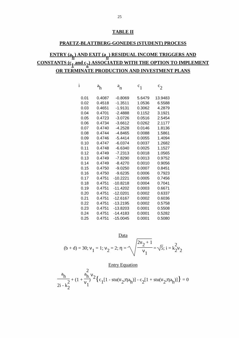
the market value of equity and the residual income stream for the Praetz-Blattberg-Gonedes processes, by employing a simple numerical example. We thus continue with

18

the assumption of the previous section that the book value of the firm’s equity plus decommissioning costs are (b + d) = 30. In addition, however, we also assume that ν1 = 1

and ν2 = 1 + β

k22

= 2. Since, by an earlier assumption i = β + k22, this also implies

i = k22ν2 = 2k

22. The entry, ah, and exit, an, residual income triggers and the constants, c1

and c2, associated with the option to implement or terminate the firm’s production and

investment plans for this example, are summarised in Table II. Probably the most

________________________________________________

TABLE TWO ABOUT HERE

________________________________________________

striking feature of this Table is that the entry residual income trigger, ah, quite quickly

converges towards an asymptotic value (of about 0.475) whereas the exit residual income trigger, an, continuously declines as the rate of discount increases. Whether this is a

“quirk” of the particular example employed is an interesting question which, because of space limitations, we cannot address in further detail here. The important point we wish to stress is that a firm’s ability to implement or terminate its production and investment plans has a potentially significant (and non-linear) impact on its equity value. Thus, we can consider, for example, a firm whose cost of equity is 10% and which is operating marginally above the residual income level, an = -6.0374, at which the abandonment

option will be exercised. Then from equation (22), the residual income variable reduces

equity value by an

2i - k22

= -6.0374

(2*0.1 - 0.05) = -40.25. Against this, the abandonment option

increases equity value by

c1(1 + a2n

ν1)ν2[1 - stu(ν2;

2ν2 + 1

ν1.an)] = 0.0037*(1 + 6.03742)2*2 = 10.38, or by

about a quarter of the value lost on account of the negative value of the residual income variable. Thus, it is again clear that a firm’s ability to terminate its production and investment plans has a potentially significant (and non-linear) impact on its equity value. 4. Implications for Empirical Work

The results contained in previous sections have important implications for the

increasingly popular area of empirical work based on the Garman-Ohlson structural model [Tippett and Warnock (1997), Myers (1999), Collins, Pincus and Xie (1999)]. We cannot hope to provide an exhaustive treatment of these implications here for obvious reasons and so, we focus our attention on just two of the more significant issues. The first

19

relates to the estimation of parameters of a continuous time process when the underlying variables (or more likely, transformations of them) are observed at discrete points in time only (e.g. on a yearly basis rather than continuously). Here, the focus of our attention is on estimating the speed of adjustment coefficient, β, in the stochastic differential equation (14) which, it will be recalled, relates instantaneous changes in the residual income variable, da(t), to the levels of this variable, a(t). For pedagogical reasons our analysis is based on the particular interpretation of this equation for which k2 = 0 in

which case this differential equation is known as an Uhlenbeck and Ornstein (1930) process. This is a continuous time version of the regression equation on which much of the empirical and analytical work in this area is based [Ohlson (1995, pp. 667-668), Myers (1999, p. 8)] and takes the form:

(27) da(t) = -βa(t)dt + k1dz(t)

where, as previously, β > 0 is a measure of the speed with which abnormal profits decay

away, k21 is the variance (per unit time) of instantaneous changes in the residual income

variable and dz(t) is a white noise process with unit variance parameter. Doob (1942, p. 364) shows that the solution to this differential equation takes the form:

a(1) = a(0)e-β + k1 ⌡⌠0

1

e-β(1-s)dz(s)

or, upon subtracting a(0) from both sides of this equation, in finite difference form:

(28) ∆a(0) = -(1 - e-β)a(0) + k1 ⌡⌠0

1

e-β(1-s)dz(s)

where ∆a(0) = a(1) - a(0) is the increment in the instantaneous residual income variable over the unit (annual) time period. Furthermore, we can use the procedures laid down in Cox and Miller (1965, p. 226) to show that annual increments, ∆a(0), in the instantaneous residual income variable will have a normal distribution whose mean and variance are

E0[∆a(0)] = -(1 - e-β)a(0) and Var0[∆a(0)] = k21

2β(1 - e-2β), respectively. These results

show that we can expect any abnormal profits (or losses) to dissipate at a rate which depends on the speed of adjustment coefficient, β. Higher values of β imply that abnormal profits (or losses) dissipate more quickly than will be the case for lower values of β. Now suppose, in common with much of the literature in the area [e.g. Myers (1999)], we fall into the error of using a simple discretisation of the stochastic differential equation (27) as the basis for the following time series regression equation:

20

(29) ∆q(0) = -βq(0) + ε(0) where ∆q(0) = q(1) - q(0) is the first difference in the residual income variable on which

the regression is based, q(1) = ⌡⌠0

1x(t)dt - ib(0) is the residual income earned by the firm

over the unit (annual) time period and ε(0) is a stochastic noise term which is assumed to satisfy the “standard” least squares regression assumptions. Here, it will be recalled that i is the (annual) cost of the firm’s equity capital and b(0) is the opening book value of equity and so, ib(0) will be the capital charge applicable to equity for the year beginning at time zero. Furthermore, x(t) is the instantaneous (book or accounting) earnings (on an

annualised basis) and so, ⌡⌠0

1x(t)dt will be the annual earnings figure for the year beginning

at time zero. It thus follows that q(1) = ⌡⌠0

1x(t)dt - ib(0) will be the residual income

accruing over the year beginning at time zero. Similar arguments show that the regressor

in this equation, q(0) = ⌡⌠-1

0x(t)dt - ib(-1), is the residual income accruing to equity over the

year beginning at time -1.

Now, it is clear from equations (27) and (28) that the regression procedures which underscore equation (29) involve at least two errors of fundamental importance. The first arises out of the fact that the regression equation (29) is based on the incorrect variables. Note that both equations (27) and (28) are based on the instantaneous residual income variables, a(1) = x(1) - ib(1) and a(0) = x(0) - ib(0), and not the “discrete time” residual

income variables, q(1) = ⌡⌠0

1x(t)dt - ib(0) and q(0) = ⌡⌠

-1

0x(t)dt - ib(-1). However, ever since

the work of Bartlett (1946) it has been known that approximating procedures like those which underscore equation (29), return biased estimates of the parameters on which the regression equation is based. Second, even if we abstract from this problem (and thus falsely assume that q(0) and q(1) are good instruments for a(0) and a(1)) it still remains that the regression equation itself is mis-specified. Note that the simple discretisation which underscores equation (29) implies that the regression procedures will estimate -β directly. However, as the correctly specified equation (28) makes clear it is not -β which the regression procedures will end up estimating but rather a transform of it; namely,

-(1 - e-β) = -β + 12β2 -

16β3 + ____. This means that the bias in the regression estimate of

the speed of adjustment coefficient, β, based on equation (29) will, in general, be of the

order of β2 or worse, depending on the statistical procedures used in the estimation process. It is a combination of these (and some other) errors which explains why empirically estimated models of the kind implied by equation (29) often return rationally untenable parameter estimates and/or exhibit evidence of serious model mis-specification, similar to those reported by Myers (1999).

21

We can get a rough idea of the potential errors arising out of these approximation

procedures by examining the regression model employed by Myers (1999) in further detail. Myers (1999, p. 17) uses a large sample of publicly listed American companies to estimate speed of adjustment coefficients based on regression procedures that are very similar to those which underscore equation (27). These procedures return an estimate of the median speed of adjustment coefficient for the sample of 0.766. However, the analysis which underscores equation (27) shows that if the discrete time residual income measures, q(0) and q(1), turn out to be good instruments for their instantaneous equivalents, a(0) and a(1), then the Myers (1999) regression procedures will return an

estimate for (1 - e-β) and not β itself. In other words, the “correct” estimate of the median speed of adjustment coefficient using the Myers (1999) regression procedures will be

obtained by solving the equation (1 - e-β) = 0.766 or β = -log(1 - 0.766) = 1.452. Hence, even if q(0) and q(1) do turn out to be good instruments for their instantaneous equivalents, a(0) and a(1), Myers’ (1999) empirical results indicate that there will be significant errors from employing the mis-specified regression procedures which characterise this area of the accounting literature. For Myers’ (1999) sample, the “correct” estimate of the median speed of adjustment coefficient is nearly twice that which he reports in his paper.

A second issue stems from the fact that our analysis also has relevance to the steadily increasing stream of papers which purport to estimate the cost of equity capital using equity prices, based on the assumption that the firm’s accounting policies are compatible with a clean surplus interpretation of the Garman-Ohlson structural model. The paper by Botosan (1997) for U.S. data and Butler, Holland and Tippett (1994) and O’Hanlon and Steele (2000) for U.K. data are good examples of such empirical work although Walker (1997) provides a reasonably detailed account of some of the other work conducted in the area. The conventional procedure is best demonstrated by Botosan (1997, pp. 358-359) who estimates the cost of equity capital for 122 companies using a four year “window” (commencing in 1991) based on the fact that the clean surplus requirement implies that the market value of equity is equal to its book value, b, plus the

expected present value of the residual income stream, E0[⌡⌠0

∞e-ita(t)dt]. These assumptions

return a median estimate of the cost of equity capital of about 19% (per annum) which Botosan (1997, p. 340) notes may “appear [to be] inflated”.12 However, the results she obtains are based on a model which assumes that the firm’s production and investment plans are completely irreversible. If the value of the option to terminate or reverse the firm’s investment and production plans is included in the valuation equation, however, then ceteris paribus Botosan’s (1997) procedures will under (over) estimate the cost of equity if the option value at the beginning of the four year window exceeds (is less than) the expected option value at the end of the four year window. Hence, the accuracy of

12 Using different procedures and a slightly larger sample of about 150 UK companies, Butler, Holland and Tippett (1994, p. 311) obtain a median estimate of the cost of equity of about 20%.

22

Botosan’s (1997) estimates hinge critically on their being insignificant variations in option values over the period examined in her study.13 5. Conclusions

Continuous time reformulations of the Garman and Ohlson (1980) equity valuation model show that the linear pricing technologies which characterise this area of accounting research are special cases of a more general non-linear pricing relationship. These non-linearities arise from the fact that firms have the option of terminating their production and investment plans, especially if they turn out to be “significant” loss making ventures. We demonstrate the potential significance of these non-linearities for alternative stochastic specifications of the residual income stream. The first assumes residual income follows a pure random walk (based on the normal distribution) and as such, has increments with a zero mean and constant variance. A second and in our view, more satisfactory process, however, takes the residual income stream to be generated by an elastic random walk based on the Student distributions of Praetz (1972) and Blattberg and Gonedes (1974). For these processes the variance of instantaneous increments in the residual income stream increases with its absolute value.

It is important to note, however, that our analysis is based on the simplest possible

interpretation of the Ohlson (1995) model. More general versions of the model can be developed and include “information” and other variables which are not immediately captured by the firm’s accounting system. Whilst the inclusion of these variables leads to a more refined formulation of the irreversibility problem, our preliminary analysis shows that the technical demands associated with such models goes far beyond anything contained in the present paper. Thus, a useful area for future research would be to explore whether there are parsimonious ways of generalising the models summarised here so that they accommodate these other variables in a relatively simple manner. Our analysis also has relatively little to say about some important “supply side” issues; in particular, how the factor and product markets available to the firm shape its capital expenditure decisions and how these, in turn, might be consistent with residual income streams based on the normal and Student distributions. The potential inconsistencies which can arise from partially developed supply side models are well documented in the literature [Merton (1973, pp. 870-871), Cox, Ingersoll and Ross (1985, pp. 385-387)] and means that this might also be a fruitful area of future research.

Another possible improvement stems from the fact that the two stochastic

processes employed in our analysis are based on a form “unbiased” accounting. By this we mean our assumptions imply that residual income gravitates towards a long term mean of zero and so, on average we can expect unrecorded goodwill to be zero. Whilst this is a particularly useful assumption from a pedagogical and expositional point of view, intuition suggests it is unlikely to be the case in general. However, amending our analysis to permit “biased” accounting requires that we invoke stochastic processes which are much more complicated than those contained in the text and so, pedagogical considerations dictate that we leave both this and the other issues raised in this section to the capable hands of future researchers.

13 Similar criticisms apply to the Butler, Holland and Tippett (1994) study.

23

TABLE I

PURE RANDOM WALK

ENTRY (ah) AND EXIT (an) RESIDUAL INCOME TRIGGERS AND

CONSTANTS (c1 and c2) ASSOCIATED WITH THE OPTION TO IMPLEMENT

OR TERMINATE PRODUCTION AND INVESTMENT PLANS

i ah an c1 c2

0.01 1.8429 -2.1429 184.2934 170.9770 0.02 2.2587 -2.8587 88.9585 76.5673 0.03 2.5266 -3.4266 57.8383 46.1848 0.04 2.7241 -3.9241 42.5381 31.5130 0.05 2.8795 -4.3795 33.4904 23.0176 0.06 3.0063 -4.8063 27.5360 17.5577 0.07 3.1126 -5.2126 23.3322 13.8023 0.08 3.2031 -5.6031 20.2128 11.0930 0.09 3.2813 -5.9813 17.8103 9.0683 0.10 3.3496 -6.3496 15.9058 7.5134 0.11 3.4097 -6.7097 14.3607 6.2934 0.12 3.4629 -7.0629 13.0834 5.3193 0.13 3.5102 -7.4102 12.0105 4.5303 0.14 3.5527 -7.7527 11.0973 3.8834 0.15 3.5908 -8.0908 10.3110 3.3475 0.16 3.6251 -8.4251 9.6273 2.8997 0.17 3.6562 -8.7562 9.0275 2.5226 0.18 3.6843 -9.0843 8.4974 2.2029 0.19 3.7099 -9.4099 8.0254 1.9302 0.20 3.7331 -9.7331 7.6028 1.6964 0.21 3.7544 -10.0544 7.2222 1.4951 0.22 3.7738 -10.3738 6.8778 1.3209 0.23 3.7915 -10.6915 6.5646 1.1696 0.24 3.8077 -11.0077 6.2786 1.0379 0.25 3.8226 -11.3226 6.0166 0.9227

Data

(b + d) = 30; η = 2iσ =

14

Entry Equation

ahi + c2exp(-ηah) = c1exp(ηah)

Exit Equation

(b + d) + ani + c2exp(-ηan) = c1exp(ηan)

24

Smooth Pasting Conditions

ah, an = 1η.log[ 1

2c1ηi ± 1

4c21η2i2

– c2c1

]

25

TABLE II

PRAETZ-BLATTBERG-GONEDES (STUDENT) PROCESS

ENTRY (ah) AND EXIT (an) RESIDUAL INCOME TRIGGERS AND

CONSTANTS (c1 and c2) ASSOCIATED WITH THE OPTION TO IMPLEMENT

OR TERMINATE PRODUCTION AND INVESTMENT PLANS

i ah an c1 c2

0.01 0.4087 -0.8069 5.6479 13.9483 0.02 0.4518 -1.3511 1.0536 6.5588 0.03 0.4651 -1.9131 0.3062 4.2879 0.04 0.4701 -2.4888 0.1152 3.1921 0.05 0.4723 -3.0726 0.0516 2.5454 0.06 0.4734 -3.6612 0.0262 2.1177 0.07 0.4740 -4.2528 0.0146 1.8136 0.08 0.4744 -4.8465 0.0088 1.5861 0.09 0.4746 -5.4414 0.0055 1.4094 0.10 0.4747 -6.0374 0.0037 1.2682 0.11 0.4748 -6.6340 0.0025 1.1527 0.12 0.4749 -7.2313 0.0018 1.0565 0.13 0.4749 -7.8290 0.0013 0.9752 0.14 0.4749 -8.4270 0.0010 0.9056 0.15 0.4750 -9.0250 0.0007 0.8451 0.16 0.4750 -9.6235 0.0006 0.7923 0.17 0.4751 -10.2221 0.0005 0.7456 0.18 0.4751 -10.8218 0.0004 0.7041 0.19 0.4751 -11.4202 0.0003 0.6671 0.20 0.4751 -12.0201 0.0002 0.6337 0.21 0.4751 -12.6167 0.0002 0.6036 0.22 0.4751 -13.2195 0.0002 0.5758 0.23 0.4751 -13.8203 0.0001 0.5508 0.24 0.4751 -14.4183 0.0001 0.5282 0.25 0.4751 -15.0045 0.0001 0.5080

Data

(b + d) = 30; ν1 = 1; ν2 = 2; η = 2ν2 + 1

ν1 = 5; i = k

22ν2

Entry Equation

ah

2i - k22

+ (1 + a2h

ν1)ν2{c1[1 - stu(ν2;ηah)] - c2[1 + stu(ν2;ηah)]} = 0

26

Exit Equation

(b + d) + an

2i - k22

+ (1 + a2n

ν1)ν2{c1[1 - stu(ν2;ηan)] - c2[1 + stu(ν2;ηan)]} = 0

Smooth Pasting Conditions

Determine the ah and an which satisfy the following condition:

2aν2ν1

(1 + a2

ν1)ν2-1

{c1[1 - stu(ν2;ηa)] - c2[1 + stu(ν2;ηa)]} + 1

2i - k22

= 2(c1 + c2)Γ(ν2 + 1)

πν1.Γ(2ν2 + 1

2 ).(1 +

a2

ν1)-1

27

APPENDIX Series Expansion for the Value of the Option to Reverse Production and Investment

Plans for a Mean Reversion Process Based on the Student Distribution (Praetz-Blattberg-Gonedes Process)

In the text we showed that the benefits which accrue from being able to terminate

or reverse the firm’s investment and production plans, φ(a), are determined by solving the differential equation (17):

12(k

21 + k

22a2)φ"(a) - βa φ'(a) - iφ(a) = 0

Suppose we seek a solution of the form φ(a) = ∑j=0

∞ αja

j, where the αj are parameters to be

determined. Now since φ'(a) = ∑j=0

∞ jαja

j-1 and

φ"(a) = ∑j=0

∞ j(j-1)αja

j-2 = ∑j=0

∞ (j+2)(j+1)αj+2aj are the first and second derivatives of this

solution we can substitute into the differential equation to give:

∑j=0

∞ {1

2(j+2)(j+1)k21αj+2 +

12j(j-1)k

22αj - jβαj - iαj}aj = 0

Thus, the coefficient associated with aj must be zero, or:

αj+2 = {2(jβ + i) - j(j-1)k

22

(j+2)(j+1)k21

}αj

Letting j assume only even integral values leads to equation (18a), the first complementary series expansion contained in the text for the Praetz-Blattberg-Gonedes process, whilst letting j assume odd integral values leads to equation (18b), the second complementary series expansion.

28

REFERENCES Anderson, T., An Introduction to Multivariate Statistical Analysis, New York: John Wiley & Sons, Inc., 1958. Bartlett, M., “On the Theoretical Specification and Sampling Properties of Autocorrelated Time Series”, Journal of the Royal Statistical Society Supplement, 8, 1 (January 1946), pp. 27-41. Bergstrom, A., Continuous Time Econometric Modelling, Oxford: Oxford University Press, 1990. Bernard, V., “Accounting Based Valuation Methods, Determinants of Market-to-Book Ratios, and Implications for Financial Statement Analysis”, Working Paper, University of Michigan, 1994. Biekpe, N., M. Tippett and R. Willett., “Accounting Earnings, Permanent Cash Flow and the Distribution of the Earnings to Price Ratio”, British Accounting Review, 30, 2 (June 1998), pp. 105-140. Blattberg, R. and N. Gonedes., “A Comparison of the Stable and Student Distributions as Statistical Models for Stock Prices”, Journal of Business, 47, 2 (April 1974), pp. 244-280. Botosan, C., “Disclosure Level and the Cost of Equity Capital”, Accounting Review, 72, 3 (July 1997), pp. 323-349. Boyce, W. and R. DiPrima., Elementary Differential Equations and Boundary Value Problems, New York: John Wiley & Sons, Inc., 1969. Burgstahler, D. and I. Dichev., “Earnings, Adaptation and Equity Value”, Accounting Review, 72, 2 (April 1997), pp. 187-215. Butler, D., K. Holland and M. Tippett., “Economic and Accounting (Book) Rates of Return: Application of a Statistical Model”, Accounting and Business Research, 24, 96 (Autumn 1994), pp. 303-318. Carnahan, B., H. Luther and J. Wilkes., Applied Numerical Methods, New York: John Wiley & Sons, Inc., 1969. Chambers, M., “Discrete Time Representation of Stationary and Non-Stationary Continuous Time Systems”, Journal of Economic Dynamics and Control, 23, 4 (February 1999), pp. 619-639. Collins,D., M. Pincus and H Xie., “Equity Valuation and Negative Earnings: The Role of Book Value of Equity”, Accounting Review, 74, 1 (January 1999), pp. 29-61. Cox, J., J. Ingersoll and S. Ross., “A Theory of the Term Structure of Interest Rates”, Econometrica, 53, 2 (March 1985), pp. 385-407.

29

Cox, D. and H. Miller., The Theory of Stochastic Processes, London: Chapman and Hall, 1965. Dechow, P., A. Hutton and R. Sloan., “An Empirical Assessment of the Residual Income Valuation Model”, Journal of Accounting and Economics, 26, 1 (January 1999), pp. 1-34. Dixit, A. and R. Pindyck., Investment Under Uncertainty, Princeton, New Jersey: Princeton University Press, 1994. Doob, J., “The Brownian Movement and Stochastic Equations”, Annals of Mathematics, 43, 2 (April 1942), pp. 351-369. Edey, H., “Business Valuation, Goodwill and the Super-Profit Method”, in Baxter, W. and S. Davidson., Studies in Accounting Theory, London: Sweet & Maxwell Limited, 1962, pp. 201-217. Freund, J. and R. Walpole., Mathematical Statistics, Englewood Cliffs, New Jersey: Prentice-Hall, Inc., 1987. Garman, M. and J. Ohlson., “Information and the Sequential Valuation of Assets in Arbitrage Free Economies”, Journal of Accounting Research, 18, 2 (Autumn, 1980), pp. 420-440. Hamilton, J., Time Series Analysis, Princeton: Princeton University Press, 1994. Karlin, S. and H. Taylor., A Second Course in Stochastic Processes., New York: Academic Press, Inc., 1981. Lahiri, K., “The ET Interview: Professor G. S. Maddala”, Econometric Theory, 15, 5 (October 1999), pp. 753-776. Lo, A., “Maximum Likelihood Estimation of Generalized Itô Processes with Discretely Sampled Data”, Econometric Theory, 4, 2 (August 1988), pp. 231-247. Merton, R., “An Intertemporal Capital Asset Pricing Model”, Econometrica, 41, 5 (September 1973), pp. 867-887. Myers, J., “Implementing Residual Income Valuation with Linear Information Dynamics”, Accounting Review, 74, I, (January 1999), pp. 1-28. O’Hanlon, J. and A. Steele, “Estimating the Equity Risk Premium using Accounting Fundamentals”, Journal of Business Finance and Accounting, forthcoming. Ohlson, J., “Earnings, Book Values, and Dividends in Security Valuation”, Contemporary Accounting Research, 11, 2 (Spring 1995), pp. 661-687. Phillips, C., “The ET Interview: Professor Albert Rex Bergstrom”, Econometric Theory, 4, 2 (August 1988), pp. 301-327.

30

Praetz, P., “The Distribution of Share Price Changes”, Journal of Business, 45, 1 (January 1972), pp. 49-55. Rubinstein, M., “An Aggregation Theorem for Securities Markets”, Journal of Financial Economics, 1 (1974), pp. 225-244. Rubinstein, M., “The Valuation of Uncertain Income Streams and the Pricing of Options”, Bell Journal of Economics and Management Science, 7 (1976), pp. 407-425. Spiegel, M., Advanced Calculus, New York: McGraw-Hill Book Company, 1974. Tippett, M. and T. Warnock., “The Garman-Ohlson Structural System”, Journal of Business Finance and Accounting, 24, 7&8 (September 1997), pp. 1075-1099. Uhlenbeck, G. and L. Ornstein., “On the Theory of the Brownian Motion”, Physical Review, 36 (September 1930), pp. 823-841. Walker, M., “Clean Surplus Accounting Models and Market Based Accounting Research: A Review”, Accounting and Business Research, 27, 4 (Autumn 1997), pp. 341-355.