Resonant Mass Gravitational Wave Detectors

David BlairUniversity of Western Australia

• Historical Introduction

• Intrinsic Noise in Resonant Mass Antennas

• Transducers

• Transducer-Antenna interaction effects

• Suspension and Isolation

• Data Analysis

Sources and Materials

• These notes are about principles and not projects.

• Details of the existing resonant bar network may be found on the International Gravitational Events Collaboration web page.

• References and some of the content can be found in

• Ju, Blair and Zhou Rep Prog Phys 63,1317,2000.

• Online at www.iop.org/Journals/rp

• Draft of these notes available www.gravity.uwa.edu.au

•Sao Paulo

•Leiden

•Frascati

•Sphere developments

Existing Resonant Bar Detectors and sphere developments

  

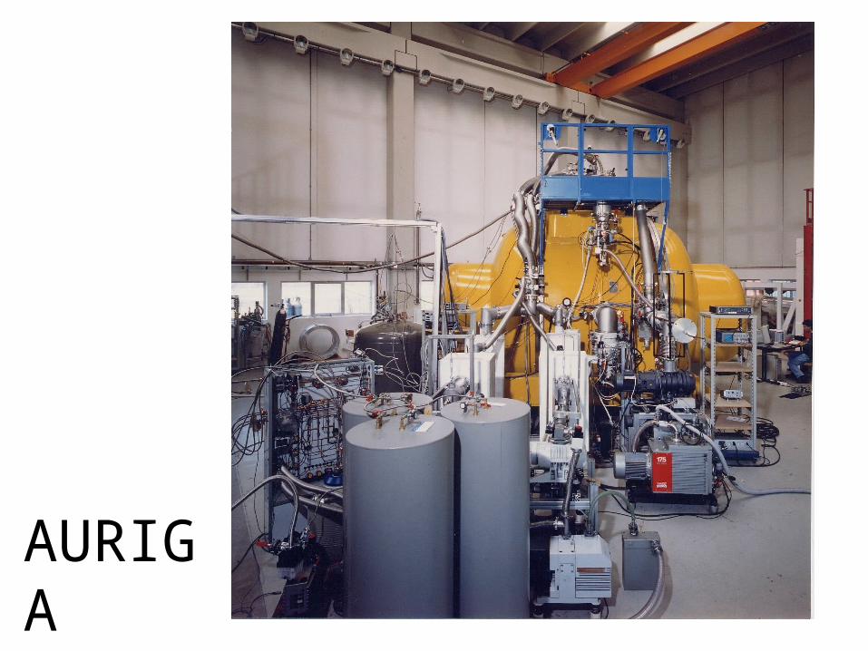
AURIGA

  

EXPLORER

Weber’s Pioneering Work• Joseph Weber Phys Rev 117, 306,1960• Mechanical Mass Quadrupole Harmonic

Oscillator: Bar, Sphere or Plate• Designs to date:

Bar

Sphere

Torsional Quadrupole Oscillator

Weber’s suggestions:

Earth: GW at 10-3 Hz.

Piezo crystals: 107 Hz

Al bars: 103 Hz

Detectable flux spec density: 10-7Jm-2s-1Hz-1

( h~ 10-22 for 10-3 s pulse)

Gravity Wave Burst Sources and Detection

223

16 hhG

cS

Energy Flux of a gravitational wave:

Short Bursts of duration g

Assume ghh /2 2

23 4

16 g

h

G

cS

J m-2 s-1

gG

h

G

cE

23 4

16

Total pulse energy density EG = S.g

J m-2 s-1

Jm-2

Flux Spectral Density

Bandwidth of short pulse: ~ 1/g

Reasonable to assume flat spectrum: F() ~ E/ g

ie: G

hcF

4)(

23 J.m-2.Hz-1

For short bursts: F() ~ 20 x 1034 h2

Gravitational wave bursts with g~10-3s were the original candidate signals for resonant mass detectors.

However stochastic backgrounds and monochromatic signals are all detectable with resonant masses.

Black Hole Sources and Short Bursts

Start with Einstein’s quadrupole formula for gravitational wave luminosity LG:

jk

jkG

dt

Dd

c

GL

2

3

3

55

where the quadrupole moment Djk is defined as: xdxxxtD jkkj

jk32

3

1

Notice: for a pair of point masses D=ML2 ,

for a spherical mass distribution D=0

for a binary star system in circular orbit D varies as sin2t

Burst Sources Continued

Notice also that represents non-spherical kinetic energy

ie the kinetic energy of non-spherically symmetric motions.

D

For binary stars (simplest non sperically symmetric source), projected length (optimal orientation) varies sinusoidally,

D~ML2sin22t,

64255

16~

LMc

GLG

32~ MLDThe numerical factor comes from the time average of the third time derivative of sin2t.

Now assume isotropic radiation

24 r

LS G

2

3

16h

G

cS

but also use

Note that KE=1/2Mv2= 1/8ML22

To order of magnitude2

22

532

r

E

c

G

c

Gh ns

andr

E

c

Gh ns

4

Maximal source: Ens=Mc2……merger of two black holes r

r

r

Mc

c

Gh s~

2

4

In general for black hole births r

rh s Here is conversion

efficiency to gravitational waves

•Weber used arguments such as the above to show that gravitational waves created by black hole events near the galactic centre could create gravitational wave bursts of amplitude as high as 10-16.

•He created large Al bar detectors able to detect such signals.

•He identified many physics issues in design of resonant mass detectors.

• His results indicated that 103 solar masses per year were being turned into gravitational waves.

•These results were in serious conflict with knowledge of star formation and supernovae in our galaxy.

•His data analysis was flawed.

•Improved readout techniques gave lower noise and null results.

Weber’s Research

Energy deposited in a resonant mass

Energy deposited in a resonant mass EG

dFEG

is the frequency dependent cross section

F is the spectral flux density

Treat F as white over the instrument bandwidth

Then dFE aG

28

c

v

c

Gmd s

Paik and Wagoner showed for fundamental quadrupole mode of bar:

x

y

zEnergy deposited in an initially stationary bar Us

Us=F(a).sin4sin22 Mc

v

c

G s 2

28

Incoming wave

Energy and Antenna Pattern for Bar

Sphere is like a set of orthogonal bars giving omnidirectional sensitivity and higher cross section

M, TA

Ta a

F

v

Z11 Z12

Z21 Z22

Se

SiG

V

Ii

Bar Transducer Amplifier Recorder

Detection Conditions

• Detectable signal Us Noise energy Un

•Transducer: 2-port device:

Current

velocity

Z

Z

Z

Z

Voltage

Force

22

12

21

11

computer

•Amplifier , gain G, has effective current noise spectral density Si and voltage noise spectral density Se

Mechanical input impedance Z11

Forward transductance Z21 (volts m-1s-1)

Reverse transductance Z12 (kg-amp-1)

Electrical output impedance Z22

X2

X1

P1P2

X1=AsinResonant

masstransducer

Vsinat ~

XG

X2=Acos

Reference oscillator

multiply

0o 90o

Bar, Transducer and Phase Space Coordinates

determines time for transducer to reach equilibrium

•X1 and X2 are symmetrical phase space coordinates

•Antenna undergoes random walk in phase space

•Rapid change of state measured by length of vector (P1,P2)

•High Q resonator varies its state slowly

Asin(at+

Bar

C

Pump Oscillator

Modulated Output

Persistent Current 1

SQUIDOutput a

Two Transducer Concepts

Parametric Direct

•Signal detected as modulation of pump frequency

•Critical requirements: low pump noise low noise amplifier at

modulation frequency

•Signal at antenna frequency

•Critical requirements: low noise SQUID amplifier low mechanical loss circuitry

Mechanical Impedance Matching

•High bandwidth requires good impedance matching between acoustic output impedance of mechanical system and transducer input impedance

•Massive resonators offer high impedance

•All electromagnetic fields offer low impedance (limited by energy density in electromagnetic fields)

•Hence mechanical impedance trasformation is essential

•Generally one can match to masses less than 1kg at ~1kHz

Mechanical model of transducer with intermediate mass resonant transformer

Resonant transformer creates two mode system

Two normal modes split byeff

a M

m

T r a n s d u c e r A s s e m b l y

B a r

B e n d in g f l a p

G lu e j o in t2 4 h r e p o x y

P u m p F r e q u e n c y : 9 .5 G H z

f / x = T u n i n g C o e f f : 3 0 0 M H z / µ m

T o a c h i e v e 9 .5 0 0 1 M H zr e q u i r e x = x 0 3 n m ( x 0 = 1 0 µ m )

Bending flap secondary resonatorMicrowave

cavity

Data Acquisition

Mixers

Phase shifters

Filter

Electronically adjustable phase shifter & attenuator

SO Filter

Phase servo

Frequency servo

W-amplifierPrimaryW-amplifier

SpareW-amplifier

Microstripantennae

Microwave interferometer

Cryogenic components

Bar

Bending flap

Transducer

RF

9.049GHz 451MHz

9.501GHz

CompositeOscillator

Microwave Readout System of NIOBÉ (upgrade)

Secondary Resonator (“mushroom”) and Transducer

Pickup Coil

DC SQUID (Amplifier. Its output is proportioanl to the motion of the mushroom)

Direct Mushroom Transducer

A superconducting persistent current is modulated by the motion of the mushroom resonator and amplified by

a DC SQUID.

Aluminium antenna

Niobium Coils

Niobium Diaphragm

Heat Switch

Heat Switch

SQUID Amplifier input coil

Pair of pick-up coils

Current supply leads

resonant superconducting diaphragm

Niobium Diaphragm Direct Transducer (Stanford)

Three Mode Niobium Transducer (LSU)

•Two secondary resonators

•Three normal modes

•Easier broadband matching

•Mechanically more complex

Three general classes of noise

Brownian Motion Noise

kT noise energy

Series Noise Back Action Noise

2

2

22

1

4

aeff

ath

M

kTx

Low loss angle compresses thermal noise into narrow bandwidth at resonance.

Decreases for high bandwidth.(small i)

Broadband Amplifier noise, pump phase noise or other additive noise contributions.

Series noise is usually reduced if transductance Z21 is high.

Always increases with bandwidth

Amplifier noise acting back on antenna.

Unavoidable since reverse transductance can never be zero.

A fluctuating force indistingushable from Brownian motion.

Noise Contributions

Total noise referred to input:

i

eeffii

effa

ian

S

Z

MS

M

ZkTU

)(2

)(2

22

21

212

Reduces as i/a because of predictability of high Q oscillator

Reduces as i/M because fluctuations take time to build up and have less effect on massive bar

Increases as M/i reduces due to increased bandwidth of noise contribution, and represents increased noise energy as referred to input

Quantum Limits

Noise equation shows any system has minimum noise level and optimum integration time set by the competing action of series noise and back action noise.

Since a linear amplifier has a minimum noise level called the standard quantum limit this translates to a standard quantum limit for a resonant mass.

Noise equation may be rewritten

where A is Noise Number: equivalent number of quanta.

The sum AB+AS cannot reduce below~1: the Standard Quantum Limit

SBTa

n AAAU

A

s

a

seff

aSQL v

kms

M

tonne

kHz

f

vMh

15.05.021

5.0

22

101

1101.1~

2

Burst strain limit~10-22 (100t sphere) corres to h()~3.10-24

Thermal Noise Limit

Thermal noise only becomes negligible for Q/T>1010 (100Hz bandwidth)

5.0

22

QvM

kTh

seff

aith

(Q=a/

5.09

2

1021 100

1.0

1010

110

B

Hz

K

T

QvM

J

kHz

fh

seffth

Thermal noise makes it difficult to exceed hSQL

Ideal Parametric Transducer

Noise temperature characterises noise energy of any system.Since photon energy is frequency dependent, noise number is more useful.Amplifier effective noise temperature must be referred to antenna frequency For example a = 2 x 700Hz pump= 2 x 9.2 GHz

Tn = 10K: Hence and Teff = 8 10-7 K

Cryogenic microwave amplifiers greatly exceed the performance of any existing SQUID and have robust performance•Oscillator noise and thermal noise degrade system noise

np

aeff TT

pump

nkTA

BPF

LOOP OSCILLATOR

Microwave Interferometer

LORF

LNA

Circulator

Phase error detector

mixer

Loop filter

Sapphire loaded cavity resonator

Qe~3107

varactor

DC Bias

W-amplifier

W-amplifier

Filtered output

+

+

Non-filtered output

Pump Oscillators for Parametric Transducer

A low noise oscillator is an essential component of a parametric transducer

A stabilised NdYAG laser provides a similar low noise optical oscillator for optical parametric transducers and for laser interferometers which are similar parametric devices.

Nb bar primary mechanical oscilator

microstrip antenas

re-entrant cavity transducer

cryogenic circulator

AM noise reduction system

low noise SLOCSC oscillator mixed with a HP 8662A synthesizer (9.5GHz)

low pass filter

output signal

room temperature low-noise amplifier

cryogenic low-noise amplifier

3dB Hybrid TEE

attenuatorphase shifter

phase tracking

quadrature channel

frequency trackingin-phase channel

carrier suppression interferometer

bending flap secondary mechanical oscillator

Two Mode Transducer Model

Coupling and Transducer Scattering Picture

a

p

+=p+a

-=p-a

?

transducer

Pump photons

Signal phonons

Output sidebands

Treat transducer as a photon scatterer

Because transducer has negligible loss use energy conservation to understand signal power flow- Manley-Rowe relations.

Note that power flow may be altered by varying asper previous slide

0

PPP

a

a

0

PPP

p

p

Formal solution but results are intuitively obvious

Upper mode Lower modeCold damping of bar modes by parametric transducer

Bar mode

frequency tuning by pump tuning

Parametric transducer damping and elastic stiffness

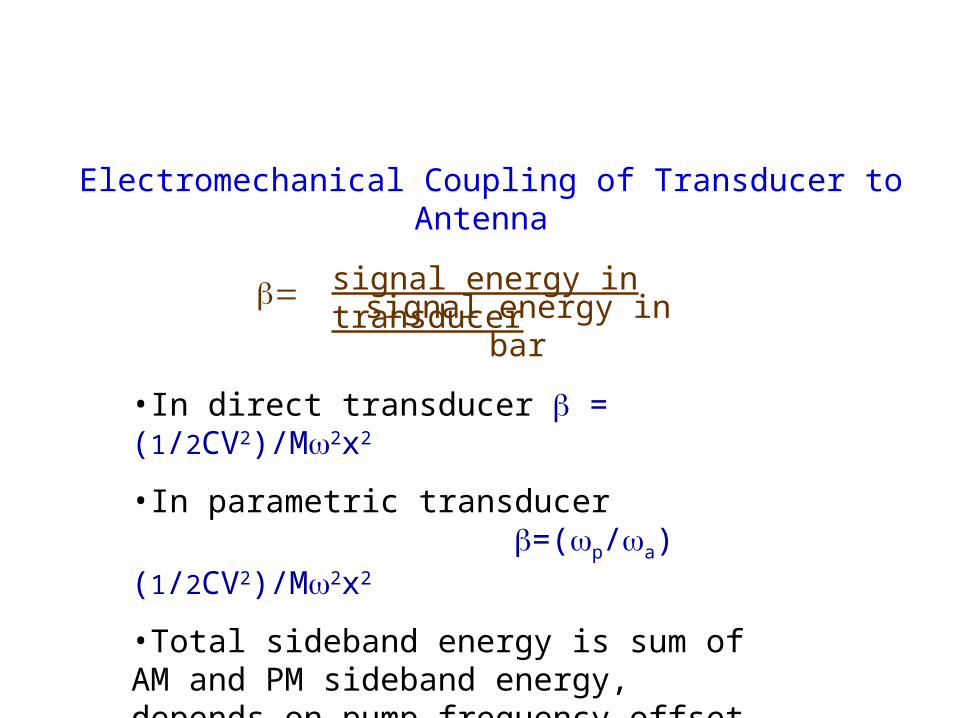
Electromechanical Coupling of Transducer to Antenna

signal energy in transducersignal energy in bar

•In direct transducer = (1/2CV2)/M2x2

•In parametric transducer =(p/a)(1/2CV2)/M2x2

•Total sideband energy is sum of AM and PM sideband energy, depends on pump frequency offset

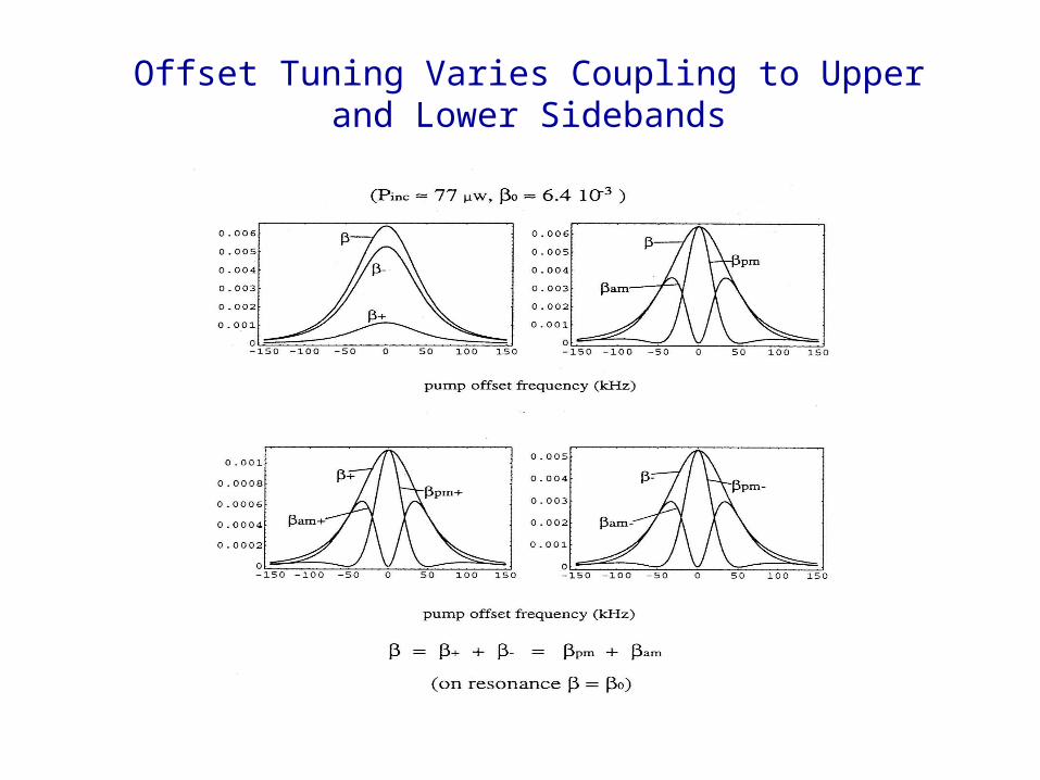
Offset Tuning Varies Coupling to Upper and Lower Sidebands

Manley-Rowe Solutions

If p>>a, Pp ~ -(P++P-).

If P+/+ < P-/- ,then Pa< 0…..negative power flow…instability

If P+/+ > P-/- ,then Pa> 0…..positive power flow…cold damping

By manipulating using offset tuning can cold-damp the resonator…very convenient and no noise cost.Enhance upper sideband by operating with pump frequency below resonance.

Offset tuning to vary Q and in high Q limit

If transducer cavity has a Qe>p/a , then

b is maximised near the cavity resonance or at the sideband frequencies. Strong cold damping is achieved for p=cavity-a .

Thermal noise contributions from bar and secondary resonator

Thermal noise components for a bar Q=2 x108 (antiresonance at mid band) and secondary resonator Q=5 x 107

m2 H

z-1

Frequency Hz

bar

Secondary resonator

Low high series noise,

low back action noise

Spectral Strain

sensitivity

SNR/Hz/mK

Transducer Optimisation

This and the following curves from M Tobar

Thesis UWA 1993

Reduced Am noiseSpectral

Strain sensitivity

SNR/Hz/mK

Higher secondary mass Q-

factor

Spectral Strain

sensitivity

SNR/Hz/mK

Reduced back

action noise from pump

AM noise

Spectral Strain

sensitivity

SNR/Hz/mK

High Qe, high coupling

Spectral Strain

sensitivity

SNR/Hz/mK

Allegro Noise Theory and Experiment

Relations between Sensitivity and Bandwidth

effT

T

Q

fBandwidth

42

M

kT

v

L

f

Sh

gs

ah

g

222

)(1

Minimum detectable energy is defined by the ratio of wideband noise to narrow band noise

Express minimum detectable energy as an effective temperature

fnoisenarrowband

isewidebandnoTE 2min

Optimum spectral sensitivity depends on ratioMQ

T

Independent of readout noise

Bandwidth and minimum detectable burst depends

on transducer and amplifier

Burst detection: maximum total

bandwidth important

Search for pulsar signals (CW) in spectral minima.

More bandwidth=more sources

at same sensitivity

Stochastic background: use two detectors with coinciding spectral

minima

Improving Bar Sensitivity with Improved Transducers

High , low noise,3 mode

Two mode, low , high series noise

Optimal filter

Signal to noise ratio is optimised by a filter which has a transfer function proportional to the complex conjugate of the signal Fourier transform divided by the total noise spectral density

d

S

FjGSNR

x

)(

)()(

2

122

Fourier tfm of impulse response of displacement sensed by transducer for force input to bar

Fourier tfm of input signal force

Double sided spectral density of noise refered to the transducer displacement

Monochromatic and Stochastic Backgrounds

Both methods allow the limits to bursts to be easily exceeded.

Monochromatic (or slowly varying) : (eg Pulsar signals):Long term coherent integration or FFTVery narrow bandwidth detection outside the thermal noise bandwidth.

Stochastic Background: Cross correlate between independent detectors.

Thermal noise is independent and uncorrelated between detectors.

Allegro Pulsar Search

Niobe Noise Temperature

Excess Noise and Coincidence Analysis

Log

num

ber

of

sam

ples

Energy

Excess noiseD

etector noise

•All detectors show non-thermal noise.

•Source of excess noise is not understood

•Similar behaviour (not identical) in all detectors.

•All excess noise can be elliminated by coincidence analysis between sufficient detectors. (>4)

Measure noise performance by noise temperature.

Typically h~(few x 10-17).Tn1/2

Coincidence Statistics

rRP 1Probability of event above threshhold:

(Event rate R, resolving time r)

Prob of accidental coincidence in coincidence window c

If all antennas have same background

Hence in time ttot the number of accidental

coincidences is

Ni

iNcN RP

,1

Nc

NN RP

1 Nc

Nac RN

0 5 10 15 20

10-14

10-12

10-10

10-8

10-6

10-4

10-2

100

102

104

events/day

1 bar 1982

2 bars 1991

3 bars 1999

4 bars 1999 (not enough data)

hburst

x 1018

Improvements through coincidence analysis

Suspension Systems•General rule:Mode control. Acoustic resonance=short circuit.

• Low acoustic loss suspension: many systems.

•Low vibration coupling to cryogenics:

•Cable couplings: Taber isolators or non-contact readout

•Multistage isolation in cryogenic environment

•Room Temperature isolation stages

Dead bug

cables

Nodal point

Important tool: Finite element modelling

Suspension choices

Intermediate MassLiquid Helium

Niobium Bar

Microwave Electronics

Transducer

Conning Tower Ti alloy suspesion rod Lead/Rubber vibration isolation Non-contacting radiative heat shunt Bellows to decouple the dewar from the antenna suspension Antenna suspension supports Experimental tank suspension tube

Experimental tank

Liquid nitrogen shield30 K shield

Cryogenic cantilever suspension

Interface for electrical leads, vacuum lines and cryogenic liquids

Niobe: 1.5 tonne Niobium Antenna with Parametric Transducer

Niobe Cryogenic System

Niobe Cryogenic Vibration Isolation

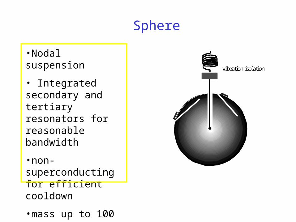
vibration isolation

•Nodal suspension

• Integrated secondary and tertiary resonators for reasonable bandwidth

•non-superconducting for efficient cooldown

•mass up to 100 tonnes

Sphere

Current limits set by bars

Bursts: 7 x 10-2 solar masses converted to gravity waves at galactic centre (IGEC)

Spectral strain sensitivity: h(f)= 6 x 10-23/Rt Hz (Nautilus)

Pulsar signals in narrow band (95 days): h~ 3 x 10-24

(Explorer)

Stochastic background: h~10-22

(Nautilus-Explorer)

Summary

Bars are well understood

Major sensitivity improvements underway

SQUIDs for direct transducers now making progress (see Frossati’s talk)

All significant astrophysical limits have been set by bars.

At high frequency bars achieve spectral sensitivity in narrow bands that is likely to exceed interferometer sensitivity for the forseeable future.