R E S E A R C H R E P O R T

Response Modifi cation for Enhanced Operation and Safety of Bridges

Andrew GastineauArturo Schultz

Steven Wojtkiewicz

Department of Civil EngineeringUniversity of Minnesota

CTS 11-14

Technical Report Documentation Page 1. Report No. 2. 3. Recipients Accession No. CTS 11-14

4. Title and Subtitle 5. Report Date

Response Modification for Enhanced Operation and Safety of Bridges

August 2011 6.

7. Author(s) 8. Performing Organization Report No.

Andrew Gastineau, Arturo Schultz and Steven Wojtkiewicz

9. Performing Organization Name and Address 10. Project/Task/Work Unit No. Department of Civil Engineering University of Minnesota 550 Pillsbury Drive, SE Minneapolis, MN 55455

CTS Project #2010037 11. Contract (C) or Grant (G) No.

12. Sponsoring Organization Name and Address 13. Type of Report and Period Covered Center for Transportation Studies University of Minnesota 200 Transportation and Safety Building 511 Washington Ave. SE Minneapolis, MN 55455

Final Report 14. Sponsoring Agency Code

15. Supplementary Notes http://www.its.umn.edu/Publications/ResearchReports/ 16. Abstract (Limit: 250 words)

This report shows that safe extension of the service life of existing bridge structures is possible through bridge health monitoring and structural response modification. To understand bridge health monitoring and structural response modification and control, it is necessary to examine: 1) common bridge vulnerabilities, 2) bridge loading models, 3) response modification devices, and 4) bridge monitoring systems. The efficacy of response modification techniques on a realistic bridge system were demonstrated using the Cedar Avenue Bridge in Minnesota as a specific example. The Cedar Avenue Bridge is a steel tied arch bridge which means that it is fracture critical. Due to the non-redundant nature of a fracture critical bridge, fatigue failure could be catastrophic and is of concern. Previous research has shown that stress concentrations exist at the joints where the hangers and floor beams are attached to the box girder [7]. Using a simulation of response modification on the Cedar Avenue Bridge model, stress ranges have been reduced on these specific details that are of concern. Modeling using a scissor jack and simple damping device has shown that stress ranges can be reduced by approximately 39% which can lead to life extension of as much as 346%.

17. Document Analysis/Descriptors

Crash analysis software, Software, Crash phases, Accident analysis, Accident data, Incident management

18. Availability Statement No restrictions. Document available from: National Technical Information Services, Alexandria, Virginia 22312

19. Security Class (this report) 20. Security Class (this page) 21. No. of Pages 22. Price Unclassified Unclassified 54

Response Modification for Enhanced Operation and Safety of Bridges

Final Report

Prepared by:

Andrew Gastineau Arturo Schultz

Steven Wojtkiewicz

Department of Civil Engineering University of Minnesota

August 2010

Published by:

Center for Transportation Studies University of Minnesota

200 Transportation & Safety Building 511 Washington Avenue SE

Minneapolis, Minnesota 55455 This report represents the results of research conducted by the authors and does not necessarily represent the views or policies of the University of Minnesota. The authors and the University of Minnesota do not endorse products or manufacturers. Any trade or manufacturers’ names that may appear herein do so solely because they are considered essential to this report.

Acknowledgments

The authors would like to extend their appreciation to the Center for Transportation Studies for supporting this work. The authors would also like to thank David Thompson for the use of his SAP2000 numerical model of the Cedar Avenue Bridge. In addition, the authors are grateful to Professor Richard Christenson of the University of Connecticut for his advice on structural control of bridges.

Table of Contents

Chapter 1: Introduction ............................................................................................................. 1

1.1 Discussion of Infrastructure ............................................................................................ 1

1.2 Motivation for Project ..................................................................................................... 1

1.3 Outline of Report ............................................................................................................ 1

Chapter 2: .... Overview of Bridge Monitoring and Structural Response Modification Components......................................................................................................................................................... 3

2.1 Common Bridge Vulnerabilities ..................................................................................... 3

2.1.1 Bridge Failures ............................................................................................................ 3

2.1.2 Recent Bridge Vulnerabilities and Deterioration ........................................................ 7

2.2 Bridge Loading ............................................................................................................. 10

2.3 Modification Devices .................................................................................................... 11

2.4 Health Monitoring Systems .......................................................................................... 13

Chapter 3: Development of Mathematical Models ................................................................. 17

3.1 Common Bridge Vulnerabilities ................................................................................... 17

3.1.1 Bridge Life Expectancy ............................................................................................ 17

3.1.2 Bridge Vulnerability Mathematical Formulations .................................................... 19

3.2 Bridge Loading Models ................................................................................................ 20

3.3 Control Devices ............................................................................................................ 21

3.3.1 Magneto-rheological Damping Devices ................................................................... 21

3.3.2 Scissor Jack Amplification Device ........................................................................... 23

3.3.3 Simple Finite Element Scissor Jack Analysis ........................................................... 30

3.4 Bridge monitoring systems ........................................................................................... 31

3.4.1 Control System Monitoring ...................................................................................... 32

3.4.2 Stress Reduction Verification Monitoring ................................................................ 32

Chapter 4: Response Modification Techniques Example ....................................................... 33

4.1 Vulnerable Bridge Selection ......................................................................................... 33

4.2 Scissor Jack Parameter Study ....................................................................................... 35

4.3 Cedar Avenue Bridge Modified with Scissor Jack Device Example ........................... 37

4.4 Cedar Avenue Bridge Example Conclusions ................................................................ 40

Chapter 5: Summary and Conclusions ................................................................................... 41

References ..................................................................................................................................... 43

List of Tables

Table 2.1 Steel details with fatigue problems ................................................................................. 9

Table 2.2 Common health monitoring systems ............................................................................ 15

Table 3.1 Stress resistance constants by detail category ............................................................... 18

Table 3.2 Nominal stress thresholds by detail category ............................................................... 18

Table 3.3 Bridge skew constants for Lindberg stress concentration formula ............................... 19

Table 3.4 Analytic and SAP2000 results for scissor jack stiffening device ................................. 30

Table 4.1 Scissor jack parameter study results ............................................................................. 36

Table 4.2 Moment envelope at vulnerable joint on the Cedar Avenue Bridge with different scissor jack configurations ............................................................................................................ 39

List of Figures

Figure 1.1 Structural response modification flowchart for addressing problematic details ........... 2

Figure 3.1 AASHTO standard truck (www.tfhrc.gov) ................................................................. 21

Figure 3.2 Magneto-rheological device [28] ................................................................................ 22

Figure 3.3 Bingham plasticity model [28] .................................................................................... 23

Figure 3.4 Mechanical device used to approximate system [28] .................................................. 23

Figure 3.5 Scissor jack configuration (not to scale) on a simple beam ........................................ 24

Figure 3.6 Deformed scissor jack configuration (not to scale) with damper on a simple beam ... 24

Figure 3.7 Forces within the scissor jack due to spring placed across the jack ............................ 27

Figure 3.8 Moments imparted on the system due to a scissor jack with a spring ......................... 27

Figure 3.9 Deflections for beam with 𝜸 = 𝟓.𝟖𝟏𝟗 and without rotational springs ....................... 29

Figure 3.10 Moments for beam with 𝜸 = 𝟓.𝟖𝟏𝟗 and without rotational springs ........................ 29

Figure 3.11 SAP2000 scissor jack with fully restrained moment connections configuration ...... 31

Figure 3.12 SAP2000 scissor jack with fully restrained moment connections moment results ... 31

Figure 3.13 SAP2000 scissor jack with truss connections configuration ..................................... 31

Figure 3.14 SAP2000 scissor jack with truss connections moment results .................................. 31

Figure 4.1 Elevation view of the Cedar Avenue Bridge [7] ......................................................... 34

Figure 4.2 Moment distribution in global SAP2000 model for dead load [7] .............................. 34

Figure 4.3 Moment distribution in global SAP2000 model for dead and live load [7] ................ 34

Figure 4.4 Von Mises stresses at L3 connection (box girder exterior) [7] ................................... 35

Figure 4.5 Von Mises stresses at L3 connection (box girder interior) [7] .................................... 35

Figure 4.6 Cedar Avenue Bridge showing the scissor jacks in 3D ............................................... 37

Figure 4.7 Cedar Avenue Bridge with scissor jack placed across one joint ................................. 37

Figure 4.8 Cedar Avenue Bridge with scissor jack placed across two joints ............................... 38

Figure 4.9 Moment range diagram for the Cedar Avenue Bridge with a scissor jack placed across the vulnerable region ..................................................................................................................... 40

Executive Summary

This report shows that safe extension of the service life of existing bridge structures is possible through bridge health monitoring and structural response modification. To understand bridge health monitoring and structural response modification and control, it is necessary to examine the components of these systems: 1) common bridge vulnerabilities, 2) bridge loading models, 3) response modification devices, and 4) bridge monitoring systems.

Information on common bridge vulnerabilities is readily available. For example, Akesson recently documented 20 catastrophic bridge failures that have occurred throughout the world over the past 150 years, and, in the process, identifies some of the most dangerous bridge vulnerabilities [1]. Many of these significant failures led to changes in bridge design and maintenance such as the implementation of inspection practices. Additionally, a report by Lindberg and Schultz [6] enumerates the vulnerabilities associated with steel details. A subsequent survey completed by 15 departments of transportation across the U.S. was used to define the frequency of occurrence of these details. Details such as cover plates and web gaps (distortional fatigue) are both common and problematic and are a focus of this report.

The most widely used bridge loading model is the standard AASHTO truck. According to the AASHTO specifications [23], this truck is used to calculate bridge fatigue life. Other loading models exist as well using equipment such as weigh in motion (WIM) to obtain more realistic truck weights for a particular roadway or bridge. One report found that for one set of WIM data in Minnesota the average truck weight was 60 kips; additionally, the same report found that increasing truck weight by 10% could reduce fatigue life by 25% or more [10].

Response modification devices, another necessary component of the proposed approach, can be broken down into passive, semi-active, and active devices. Though many structural response modification techniques have been applied to earthquake response mitigation, these can also be applied to bridge structures under service loads equally as well. These techniques have been described in [17] and are mainly applied to earthquake response applications. Passive devices include retrofits, repairs, and damping or stiffening devices that are incorporated into the bridge and have permanent characteristics and consume no power. Semi-active devices include damping and stiffening devices that have adaptable parameters that can be manipulated to change bridge response due to variable loading conditions while using small amounts of power. Active devices include damping and stiffening devices that provide large controlling forces and consume large amounts of power, but are the most versatile for applying control forces. For bridge response modification, it has been suggested in [14] and [15] that semi-active devices are most applicable and the authors of this report agree with that assessment as their small required power consumption is essential for bridge response modification.

Bridge health monitoring systems are becoming more widely used to better understand bridge response. Bridge health monitoring can be used to verify assumed responses to known loadings, monitor specific members locally, or monitor the global health of the structure. These systems can be for short-term, long-term or inspection purposes [20]. Multiple reports help to enumerate the commercial availability and capabilities of different types of bridge health monitoring equipment [20], [21]. Some relevant technologies such as accelerometers, acoustic emission,

strain gauges, global positioning system (GPS) devices, and fatigue sensing devices, among others could be helpful for response modification and control.

To be able to formulate bridge models to simulate control design, mathematical models for each of the four components described previously have been defined and described. For problematic details, remaining fatigue life has been defined in [22]. The fatigue life depends on the stress ranges experienced by a particular detail, the stress concentrations of a particular detail, and the average daily truck traffic. Interestingly, the fatigue life is inversely proportional to the cube of the stress range experienced by the detail so a small decrease in the stress range can have a large impact on fatigue life. Cover plates and web gaps both have stress concentration equations to estimate the stress ranges experienced by the detail [6], [24], [25], [26], [27].

The mathematical concepts behind general bridge loading models have been well defined by AASHTO [23] and the AASHTO standard truck serves as the best starting point unless more refined data is available. For modeling purposes, SAP2000 can apply dynamic loads to gain the best understanding of bridge response behavior. Once analysis has been completed, bridge member stress range envelopes can be reported in SAP2000 to identify stress ranges experienced by a particularly vulnerable detail.

The mathematical formulation for the modification devices needs to be understood as well. One device called a scissor jack that can aid in bridge response modification has been suggested by researchers at the University of Connecticut [15] and has previously been applied to frames in earthquake applications [29]. The scissor jack device amplifies the relatively small bridge displacements into larger displacements to allow for larger control forces from semi-active or passive damping and stiffness devices. The scissor jack has a magnification factor that depends on the geometry of the device and an expression for that factor has been derived. One control device that could be placed in the scissor jack, that has been tested for large-scale applications, and that has a well-defined loading history, is the magneto-rheological damper [28]. This device uses variable currents to create variable magnetic fields in a fluid that can control stiffness and damping parameters. Using this device, the scissor jack can impart variable control forces on the structure to reduce stress ranges and safely extend bridge life.

For response modification, bridge health monitoring systems have two goals: (1) provide feedback for the response modification control system in the form of device forces and global bridge behavior and (2) provide verification that stress ranges are being reduced at the vulnerable detail. Bridge specifics will govern monitoring system specifications, but most global behavior can be reported reliably by accelerometers and local behavior by load transducers and strain measurements.

The efficacy of response modification techniques on a realistic bridge system has been demonstrated using the Cedar Avenue Bridge in Minnesota as a specific example. The Cedar Avenue Bridge is a steel tied arch bridge which means that it is fracture critical. Due to the non-redundant nature of a fracture critical bridge, fatigue failure could be catastrophic and is of concern. Previous research has shown that stress concentrations exist at the joints where the hangers and floor beams are attached to the box girder [7]. Using a simulation of response modification on the Cedar Avenue Bridge model, stress ranges have been reduced on these specific details that are of concern. Modeling using a scissor jack and simple damping device

has shown that stress ranges can be reduced by approximately 39%, which can lead to life extension of as much as 346%.

1

Chapter 1: Introduction

1.1 Discussion of Infrastructure

Many of the bridges in the United States are being used beyond their initial design intentions, classified as structurally deficient, and are in need of rehabilitation or replacement. According to Minnesota Department of Transportation (Mn/DOT) records, as of July 2010, 270 trunk highway bridges in Minnesota are classified as structurally deficient or obsolete. Of those, 99 are structurally deficient signifying that one or more members or connections of the bridge should be repaired or replaced in the near future. Additionally, according to the Federal Highway Administration (FHWA), out of the 13,108 local and trunk highway bridges in Minnesota, 1,537 bridges are structurally deficient or functionally obsolete. The majority of these bridges were built in the 1950s and 60s and are at or near the end of their intended design life. This situation prompts one to pose the questions: How can bridge owners extend the life of these bridges while funds are allocated for bridge replacement? What options are both safe and affordable?

1.2 Motivation for Project

A large portion of bridges that are structurally deficient have details that are prone to fatigue damage. Due to the fiscal constraints of many bridge owners, the replacement of these bridges is cost prohibitive and it will be necessary to extend the life of these bridges in a safe and cost effective manner. The service life of these fatigue prone details is governed by the size and number of cyclic stress ranges experienced by the detail. As a result, if the stress ranges encountered by the detail can be reduced, the safe extension of bridge life can be accomplished. This report aims to show that by using bridge health monitoring and structural response modification techniques, stress range reduction can be achieved to safely extend bridge life.

1.3 Outline of Report

Chapter 2 presents an overview of bridge health monitoring and structural response modification to better understand the needs and components of health monitoring and control strategies. The chapter addresses previous research in four main categories: 1) common bridge vulnerabilities, 2) bridge loading models, 3) response modification devices, and 4) bridge monitoring systems, which are critical elements for successful bridge monitoring and response reduction. Figure 1.1 depicts the interactions between the four components.

Chapter 3 examines the mathematical expressions for the four parts of bridge health monitoring and structural modification addressed in this project: 1) common bridge vulnerabilities, 2) bridge loading, 3) response modification devices and 4) bridge monitoring systems. Defining these mathematical models allows for deterministic modeling to be formulated and analyses carried out. Without understanding of each component of the system, defining properties in the analysis would be difficult.

Chapter 4 demonstrates the efficacy of response modification techniques on a realistic bridge system using the Cedar Avenue Bridge in Minnesota as a specific example. The Cedar Avenue Bridge is a tied arch bridge which means that it is fracture critical. Due to the non-redundant nature of a fracture critical bridge, fatigue failure could be catastrophic and is of concern. Using

2

response modification on the Cedar Avenue Bridge, it is shown that stress ranges can be reduced on specific details that are of concern.

Figure 1.1 Structural response modification flowchart for addressing problematic details

3

Chapter 2: Overview of Bridge Monitoring and Structural Response Modification Components

To successfully understand monitoring and modification techniques for the purpose of bridge safety and life extension, four main components need to be considered: 1) common bridge vulnerabilities, 2) bridge loading models, 3) modification devices, and 4) bridge monitoring systems.

2.1 Common Bridge Vulnerabilities

The identification of bridge vulnerabilities can be a difficult task because of the diversity of factors that can contribute to bridge failure. This diversity of vulnerabilities encompasses possible vehicle or barge impacts to stress concentrations caused by specific bridge details and can be problematic to classify and recognize. The goal of this section is to identify vulnerabilities that could decrease safe bridge life and that need to be monitored to maintain or extend bridge life. To help identify what vulnerabilities affect bridge safety, it is important to understand previous bridge collapses and their causes. It is also important to understand bridge components that decrease the operational life of the bridge such as fatigue prone details that limit the safe fatigue life of the bridge.

2.1.1 Bridge Failures

To understand common vulnerabilities, one must consider the factors causing collapses in the past. Historically, bridge collapses have been caused by many different issues. Most collapses have been closely researched and reasons for the collapse are generally agreed upon. In [1], Akesson outlines five key bridge collapses that have changed the way engineers think about bridges in addition to documenting many other collapses that have occurred. The key collapses identified are: the Dee Bridge in 1847, the Tay Bridge in 1879, the Quebec Bridge in 1907, the Tacoma Narrows Bridge in 1940, and the multiple box-girder bridge failures from 1969-1971. In addition to the collapses highlighted by Akesson, other bridge failures are of interest for particularly dangerous issues and have been documented by others. Some of these collapses include: the Hoan Bridge, the Silver Bridge, the Grand Bridge, and, most recently, the 35W bridge in Minneapolis, Minnesota. Each of these failures provided insight and caution into more recent bridge designs and problems.

2.1.1.1 Dee Bridge – Brittle Fracture Collapse

The Dee Bridge was one of the world’s first iron bridges. The use of new materials (something other than wood) in bridge design began in 1779 with the erection of the Ironbridge. Following its success, more iron bridges were erected including the Dee Bridge, a three span iron girder train bridge built in 1846 which incorporated tension flanges reinforced with a Queen Post truss system (tension bars attached with a pin to the girder). Prior to the bridge’s collapse, cracking had been found in the lower flanges during inspections. Upon further investigation, it was realized that the tension bars had not been properly installed and the bars were reset; however, the cracking may have been a warning that something other than improper installation might be wrong. In 1847, the bridge collapsed as a train crossed it, killing five people and the exact reason the bridge failed is still disputed. While lateral instability and fatigue cracking have been

4

proposed as potential causes of the failure, Akesson believes that repeated loadings caused the pin holes in the web plate to elongate [1]. This elongation negated the composite action of the girders and tension rods, leaving the girder to carry the entire load. Regardless of the actual cause of the collapse, multiple lessons were learned from the failure of the Dee Bridge. It was realized that the brittle and weak nature of cast iron in tension is undesirable; consequently, more ductile materials like wrought iron and eventually steel replaced cast iron. It was also realized that a designer’s assumptions are not always correct and that if problems such as cracking occur, all possibilities of their cause should be investigated.

2.1.1.2 Tay Bridge – Stability Issues Due to Load Combinations

The Tay Bridge was built in 1878 to cross the Firth of Tay in Scotland. The bridge was the longest train bridge in the world at the time and consisted of wrought iron trusses and girders supported by trussed towers [1]. In 1879, while a mail train was crossing it at night, the bridge collapsed during a storm with high winds killing 75 people. The next morning, it was realized that thirteen of the tallest spans, having higher clearances to allow for ship passage beneath, had collapsed. It was determined that wind loading had not been taken into account in the design of the bridge. The open truss latticework was assumed to allow the wind to pass through; however, it was not considered that, when loaded with a train, the surface area of the train would transfer wind loading to the structure. During the gale, the extremely top heavy portion of the bridge, upon which the train rode, acted like a mass at the end of a cantilever. The narrow piers could not withstand the lateral thrust and collapsed into the water. This collapse highlighted problems with tall structures in windy environments, which require that the stability of the structure be considered and also highlighted the need to consider the effects of load combinations.

2.1.1.3 Quebec Bridge – Buckling Failure

Construction on the cantilever steel truss Quebec Bridge began in 1900. During construction in 1907, a compression chord was found to be distorted out of plane, and the designer ordered construction to be halted [1]. However, the contractor was falling behind schedule and continued construction which resulted in a complete collapse, killing seventy-five workers. Multiple reasons led to the collapse. First, the bridge had been designed using higher working stresses than ever allowed before to save money, and second, the designers underestimated the self-weight of the steel, causing additional stresses. The combination of these two factors resulted in large stresses causing the buckling of a compression member which led to complete collapse. A new bridge was planned and erected using compression chords with almost twice the cross-sectional area to avoid buckling; however, the bridge partially collapsed again in 1916 killing an additional 13 workers. The second collapse was blamed on a weak connection detail, which was redesigned, and the bridge was finally completed in 1917. These collapses highlighted the need for not only economical, but also safe designs. Increasing working stresses without proper testing and safety investigations can lead to devastating consequences.

5

2.1.1.4 Tacoma Narrows Bridge – Stability Issues Due to Wind

The Tacoma Narrows Bridge collapse in 1940 is one of the most well known bridge collapses. A quick internet search yields multiple videos of the collapse with millions of views. The narrow and elegant suspension bridge spanned the Puget Sound, and a gale caused the bridge to begin to oscillate and slowly swing out of control. A natural frequency of the bridge was excited, causing resonance and large deflections. The flexible nature of suspension bridges needed to be reconsidered and it was realized that a roadway needed to be stiff both laterally and vertically. The bridge had been designed to withstand a static wind pressure three times the one that resulted in collapse, but the dynamic effects of the wind loading on the bridge had not been taken into account. According to Akkeson, vortices formed on the leeward side of the deck causing oscillations at a natural frequency of the bridge to begin [1]. After the collapse, the bridge was rebuilt with a wider bridge deck and deeper girders to yield a much stiffer design . The new bridge was also tested in a wind tunnel prior to erection. These design changes helped form the standard for future suspension bridges.

2.1.1.5 Various Box-Girder Failures – Local Buckling Failures

A series of box-girder bridge failures occurred in the late 1960s and early 1970s with the majority of failures occurring during erection [1]. In 1969, the Fourth Danube Bridge in Austria experienced a buckling failure on the evening the bridge was completed. The cantilever method had been used during erection which caused high moment regions at the supports. As the final piece was placed to close the gap between the two segments, the piece had to be shortened on the top due to the sag of the cantilevers. The inner supports needed to be lowered to reduce the stress distribution to the designed continuous span distribution; however, this was to be completed the next day. As the bridge cooled that evening, tension was introduced in the shortened region and compression in the bottom flange. Areas designed to be in tension for in-service loads were instead in compression, causing buckling failures. The bridge never fully collapsed due to the inherent redundancies in a continuous girder system and was repaired. Four other box girder failures occurred in the next four years, one of which was kept secret for over 20 years. These other failures also had buckling issues during erection. Because of the large amount of collapses in a small period of time, it was clear that erection loads and practices needed to be included in the design process and that local buckling problems were not well understood.

2.1.1.6 Cosens Memorial Bridge – Brittle Fracture Due to Structural Change

Another collapse featured in [1] is the failure of the Sgt. Aubrey Cosens VC Memorial Bridge in Ontario, Canada. This tied arch bridge built in 1960 partially collapsed in 2003 when a large truck was crossing. Previously, other pieces of the bridge had failed but had gone unnoticed and, when the truck crossed, the first three vertical hangers connecting the girder to the arch failed in succession. When the first two hangers failed, the next few were able to redistribute and carry the load; however, when the third hanger finally fractured, a large portion of the deck displaced. It was learned that the hangers were designed with the ends free to rotate, but these ends had slowly seized up over time with rust and became fixed. When fixed, they were subjected to bending, which caused hidden fracturing to occur on the portions of the hangers hidden inside the arch. Fortunately, no lives were lost in this collapse, but this failure highlights the necessity

6

of understanding initial bridge design assumptions and ensuring these original design assumptions continue to hold true.

2.1.1.7 Hoan Bridge Failure – Brittle Fracture Due to Stress Concentrations

In addition to the collapses enumerated in [1], other recent collapses have been investigated and reported as well. In 2000, the Hoan Bridge failed in Wisconsin. This steel bridge built in 1970 had full depth cracking in two of three girders, with at least some cracking in all three [2]. The cracks initiated where the diaphragm connected to the girder near the tension flange because stress concentrations led to stress levels 60% above the yield level for the steel in the girder web. Steel toughness levels met the American Association of State Highway and Traffic Officials (AASHTO) requirements, but due to the excessive stress levels, cracking occurred. Clearly, this detail led to brittle fracture, and problematic details that amplify stress levels need more attention in the future.

2.1.1.8 Silver Bridge – Cleavage Fracture in Eyebar

The Silver Bridge connecting Ohio and West Virginia was the first suspension bridge in the United States to use heat treated steel eyebars as the tension members connecting the stringers to the suspension cable [3]. The bridge was constructed in the late 1920s and collapsed in 1967 killing 46 people. During rush hour, an eyebar fractured at the head which caused a complete collapse of the bridge, and the incident led to new bridge inspection standards mandated by Congress. The eyebar chains consisted of only two bars so that if one bar failed, the other would not be able to take the additional load due to the asymmetric loading. It was also realized that a gap had been left in all of the pin joints for ease of erection, which was a perfect site for the initiation of corrosion. Also, the factor of safety for these eyebars was only 2 for ultimate loads, but the original design specification had intended a factor of safety of 2.75. The tragedy led to the adoption of systematic inspections on all bridges in the United States and made engineers painfully aware of the consequences of cutting corners on design specifications to save money.

2.1.1.9 Grand Bridge Partial Failure and I-35W Bridge Failure – Gusset Plate Design

Authors in [4] and [5] discuss gusset plate issues that have caused recent collapses. In 1996 the Grand Bridge, a suspended deck truss bridge built in 1960 near Cleveland, Ohio, suffered a gusset plate failure. The failed gusset plate buckled under the compressive load and displaced, but the bridge only shifted three inches both laterally and vertically and did not completely collapse. The bridge was closed and an investigation into the cause was initiated. The Federal Highway Administration (FHWA) found that the design thickness of the plate was only marginal and which had been decreased due to corrosion. An independent forensic team concluded that the plates had lost up to 35% of their original thickness in some areas. On the day of the failure, the estimated load compared to the design load was approximately 90 percent, and it was concluded that sidesway buckling occurred in the gusset plates. The buckling occurred because the actual load that the plates could carry was exceeded, possibly due to the deterioration of the plates. The damaged gusset plates were replaced and other plates throughout the bridge deemed inadequate were retrofitted with supporting angles. Clearly gusset plates on bridges designed during the 1960s need to be analyzed for sufficient design and load capacity strength.

7

The I-35W Bridge in Minneapolis Minnesota collapsed on August 1, 2007 killing 13 people. In [5] the author discusses the undersized gusset plates that the FHWA found to be the cause of the collapse. Due to the way the design was carried out, the design forces in the diagonal members were not correctly incorporated into the gusset plate design and significantly higher forces dominated the actual stresses in the gusset plates. These higher stresses in the undersized plates led to significant yielding under service loadings and ultimately collapse.

Engineers have learned many lessons from the bridge collapses described in this section. These lessons included considering new materials, wind stability, safety factors, local buckling, construction practices, inspections practices, and connection design flaws. Although these collapses have provided many insights into bridge design and construction, other problems that have not caused major collapses also exist.

2.1.2 Recent Bridge Vulnerabilities and Deterioration

Most recently, the collapse of the I-35W Bridge highlighted issues with the aging steel bridges that were built in the early 1960s. In addition to the problems observed from bridge collapses, recent information has been written on steel bridge vulnerabilities and issues specifically in Minnesota [6]. Other issues have been reported on concrete bridges along with safety concerns in other states as well.

Authors in [6] focus on steel fatigue issues and, although these vulnerabilities will not cause immediate collapse, the high cycle fatigue issues will reduce safe bridge life. If it is possible to retrofit these details or reduce the working stress ranges on these details, bridge life could be extended. A list of common problems with steel bridges was enumerated in [6] and is repeated in Table 2.1. The authors surveyed 15 DOTs around the country and found that transverse stiffener web gaps, insufficient cope radius, and partial length cover plates were the most common details displaying fatigue cracking. The authors also mention that diaphragm distortional fatigue (due to web gapping) is common as well. In addition, connections on the box girders of tied arch bridges, specifically the Cedar Avenue Bridge in Minnesota are known to have high stress concentrations [7]. Decreasing stresses at these particular details could and should lead to increased bridge life for aging steel girder bridges in Minnesota and throughout the U.S.

In addition to steel bridge vulnerabilities, Enright and Frangopol surveyed damaged concrete bridges, and it was found that the majority of damage was caused by corrosion issues [8]. Water ingress at deck joints caused most of the corrosion problems, and other issues were typically caused by shear cracking as opposed to flexural cracking. Deck joints (generally over supports) were found to be the most likely locations on concrete bridges to have damage and need particular attention.

Taking both steel and concrete bridge vulnerabilities into account, O’Conner describes the safety assurance plan implemented for New York State’s bridge infrastructure [9]. Bridges in the New York state inventory were rank ordered using six collapse categories: hydraulic (scour), collision, steel details, concrete details, overload, and seismic. In a separate, related program, the bridges were ranked using an additional category of deterioration.

8

By modifying bridge responses using bridge monitoring and control, the life of many bridges containing the steel and concrete bridge vulnerabilities enumerated in this section may be safely extended. This report will focus on a few specific steel details vulnerable to fatigue cracking that will be more fully developed in the next chapter.

9

Table 2.1 Steel details with fatigue problems

Steel Detail Description Collapse/Cracking Example

Partial Length Cover Plate

Welded plate to flange for increased moment resistance with fatigue issues near welds. Crack begins at plate joint and initiates into the beam flange then proceeds to web. The cover plate is one of the most common problems.

Yellow Mill Pond Bridge (Connecticut)

Transverse Stiffener Web Gap

Stiffeners used to be placed with a gap between the stiffener and bottom tension flange. Cracks begin in or near welds due to distortion. 50% of bridges with the detail have cracking.

I-480 Cuyahoga River Bridge (Ohio)

Insufficient Cope Radius

Copes with small radii have stress concentrations causing cracking.

Canadian Pacific Railroad Bridge No. 51.5 (Ontario)

Shelf Plate Welded to Girder Web

Cracking initiates near welded plate, stiffener and web girder.

Lafayette Bridge (Minnesota)

Welded Horizontal Stiffener

Insufficient welding causes a fatigue crack that propagates as a brittle failure.

Quinnipiac River Bridge (Connecticut)

Stringer or Truss floor beam Bracket

Suspension bridges and truss bridges have seen issues of cracking in the beam floor bracket near expansion joints.

Walt Whitman Bridge (Delaware River)

Haunch Insert Cracks began near a poor transverse weld. However, at point near zero moment so generally not a large issue (many cycles, but low stress range).

Aquasabon River Bridge (Ontario)

Web Penetration

Cracking near backing bar of welds for beams that penetrate box stringers.

Dan Ryan Train Structure (Illinois)

Tied Arch Floor Beam

Cracks between beam flange (tie) and plate due to unexpected rotation.

Prairie Du Chien Bridge (Wisconsin)

Box Girder Corner

Continuous longitudinal weld had cold cracking in the core, undetectable to the naked eye. Fatigue caused cracking, but quite small due to small stress range.

Gulf Outlet Bridge (Louisiana)

Cantilever Floor-beam Bracket

Cracking occurs near tack welds used for construction purposes.

Allegheny River Bridge (Pennsylvania)

Cantilever: Lamellar Tear

Lamellar tear occurred in highly restrained connection. Cracks occurred prior to erection.

I-275 Bridge (Kentucky)

10

2.2 Bridge Loading

In addition to bridge vulnerabilities, bridge loading models are another crucial component necessary for the successful health monitoring and response modification of a structure. Many different types of loading for bridge structures are possible such as vehicles, earthquake loadings, vehicle impacts, in addition to other extreme events. Defining the way vehicles and other loads interact with the bridge is necessary for computer modeling of the structure. Due to the fatigue vulnerabilities of the steel details that are focused on in this report, the most important bridge loading is heavy truck loading.

French et al. reports on the modeling of heavy truck loading [10]. Therein, suggestions from NCHRP 12-51 were utilized and improved upon to refine loading and girder analysis. Truck tests were used to verify their results and beam grillage models were suggested as the easiest way to define and distribute truck loading. Finite element modeling is the best way to define truck loading but is very time consuming and generally not cost effective. The grillage method provides reasonable accuracy without overwhelming computational complexity. Additionally, the authors concluded that the truck loading defined by AASHTO seems to be fairly reasonable, but local weigh in motion (WIM) data for actual truck weights should probably be used. In Minnesota, over 70% of trucks are 5 axle trucks around the 60 kip range for weight. It may be necessary to increase this average weight depending on the types of trucks travelling over a particular bridge considering that average weights around 70 kips are possible. It was found that increasing truck weights by only 10% could reduce fatigue life by 25% and, for an increase in legal truck weight of 20%, the reduction in the remaining life in these older steel bridges could be as high as 42%.

Nowak describes the necessary components of general loading, but also states the need for better loading models for extreme events such as scour, vessel collisions, and earthquakes [11]. The dead load, or self-weight, can be subdivided into three categories: weight of premade elements, cast-in-place elements, and wearing surfaces. These are treated as bridge dependent, normal random variables. The live loadings include both static and dynamic effects from vehicles (specifically trucks) crossing the bridge and are affected by span length, position of vehicles, truck weight, axle positions and loads, and structural layout. Truck weights have a general trend, but can be very site specific, and the dynamic loads induced by the trucks depend on vehicle dynamics (shocks), bridge dynamics, and wearing surfaces. Dynamic deflection is generally constant and independent of truck weight and the extra dynamic load does not exceed 0.15 of the static live load of a single truck. Extreme loading cases such as scour, vessel collisions, and earthquakes that need to be considered are very site specific and can be quite difficult to quantify due to the rarity of occurrence and their large range of possible loading situations.

Similar to the work just discussed, Nowak describes bridge loading models, but only for static live loadings [12]. The parameters that affect the live load model are: span length, position of vehicles, truck weight, axle positions and loads, structural layout (stiffness), and future bridge/traffic growth. Using a major truck survey of 10,000 heavily loaded trucks (about 2 weeks) from 1975, probabilities based on a 75 year design period were calculated. Next, three assumptions were stated for deciding whether trucks are next to one another and are heavily loaded or not. It was found that for spans less than around 100 feet, a single truck heavily loaded governs the response and for anything larger, two heavily loaded trucks govern the response. A

11

similar study was performed for two lane bridges and it was found that two heavily loaded trucks traveling side by side governs the response. The maximum moments and shears were calculated for periods of 1 day to 75 years.

Miao and Chan studied the differences in loading models around the world [13]. The authors found that countries use models consisting of a concentrated load representing the truck, a distributed load or a combination of the two. The United States uses a concentrated truck load plus a distributed load for bridge strength design; for fatigue design, a single truck is used without the distributed load. The use of WIM data was also investigated for live load design characteristics and a statistical analysis of the data was used to find design loads instead of the traditional normality assumption. In the data for Hong Kong bridges, these WIM loads were found to be less than typical design loads.

Bridge loading models can vary widely depending on which loads are most important. Truck configurations and weights are a very important characteristic for defining vehicle loadings and can be site specific. If WIM data is present for a particular bridge, this data can be used to refine the truck loading models. After choosing which vulnerabilities and loading models will be critical for a particular health bridge application, the next important step is the selection of a modification device.

2.3 Modification Devices

Response modification devices are another component necessary for monitoring and response modification of structures. It is possible to accomplish response modification and control through either passive, semi-active, or active devices. Passive devices modify bridge behavior and, once installed, become a permanent change in the bridge structure. A retrofit to stiffen a member or the replacement of a connection would be considered a passive device along with passive damping devices. Semi-active and active devices change bridge behavior as well; however, these devices have the ability to adapt to changing bridge behavior due to changes in loading conditions unlike their passive counterparts. The ability to adapt distinguishes a control device from being a more simple modification technique. Once a particular bridge vulnerability is identified, understanding these techniques will aid in the selection of the complementary modification technique.

Previously, few have used modification devices to reduce bridge response due to typical service loading. Patten et al. showed on an in-service bridge that reductions in bridge stresses due to traffic loads could be achieved through a variable stiffening device [14]. The authors in [14] attached a system with a semi-active device that could be turned on or off depending on loading conditions. In the off position, the device acted as a passive damper but in the on position, the device added a large amount of stiffness to reduce bridge deflections. The safe life of the modified bridge was extended by over 50 years.

Work in progress on semi-active control strategies has been reported by Christenson and co-workers at the University of Connecticut [15]. The equations that govern fatigue life used by AASHTO are described and it is noted that there are three ways to increase fatigue life: 1) truck traffic reduction, 2) replacing fatigue critical details, and 3) stress range reduction. Replacing the problematic details of the bridge is quite expensive and limiting truck use would be unacceptable

12

in many highway networks. Stress range reduction can be achieved by altering the dynamic response of the bridge to reduce deflections. Reduced deflections mean reduced strains and reduced stresses, which would safely extend bridge life. In the AASHTO equations, fatigue life is inversely proportional to the cube of the stress range so that decreasing stress ranges would have a profound effect. To accomplish the reduced deflections, different control devices are discussed and semi-active control applications are described as ideal due to their small power consumption and adaptable nature. Semi-active control seems to the most logical type of control system because it is both stable and uses minimal power. The system modeled involves a semi-active resettable damping system with a mass that vibrates as the bridge vibrates and helps dissipate vibratory energy in the bridge. The damper has two chambers and, when moving in one direction, the valve closes to resist movement until maximum displacement is reached. As the direction of motion reverses, the valve opens and the other valve closes to resist motion in the new direction. By dissipating some energy and adding stiffness, the deflections in the bridge can be inducing a reduced strain or, equivalently, a reduced stress. Decreasing stress ranges can lead to bridge life extension in most cases. Many of the steel bridges built in the 1960s have finite fatigue lives due to particular details included in the bridge (cover plates, welding issues, diaphragm connections, etc.). If these stress ranges can be reduced, the life of the bridge could possibly be increased to nearly infinite (in terms of fatigue life). Some generic and basic bridge configurations are modeled and deflection reductions of close to 50% were found in simulations.

Andrawes and DesRoches investigated an interesting passive device that uses an alloy called nitinol to control the unseating of girders during excessive ground motions [16]. This alloy remains elastic throughout loading while still dissipating energy and, because the alloy does not fail and remains elastic, the device can easily re-center the displaced girder joint. Typical steel restrainers can either yield or break, causing the joint to not return to the original position.

In their book, Cheng et al. focus on systems for seismic control [17]. Though not focused on bridge applications, the book provides background for passive, semi-active, and active devices. All of these devices focus on energy dissipation to decrease overall displacements. Passive devices are generally engineered to help resist either the most likely or the most dangerous loading conditions and require no external power; however, these passive devices cannot adapt to changing conditions making them act similarly to a retrofit. The passive devices described are tuned mass dampers, tuned liquid dampers, friction devices, metallic yield devices, viscoelastic dampers, and viscous fluid dampers.

Another type of energy dissipation device discussed in [17] is the semi-active device which uses minimal power and can adapt to changing bridge conditions. The semi-active systems use sensors and a control computer to change the characteristics of the system to “smartly” apply a damping force to the structure. An advantage of semi-active devices is that when power is lost, the system is still stable and acts like a passive device. Another advantage is that their required power can be supplied by battery power which is advantageous at a bridge site. The semi-active devices described are mass dampers, liquid dampers, friction dampers, vibration absorbers, stiffness control devices, electro-rheological dampers, magneto-rheological dampers, and viscous fluid dampers.

The third type of damping system discussed in [17] involves active devices which require external power and generally use heavy equipment. Active systems are usually more expensive

13

than passive or semi-active systems but can control multiple vibration modes simultaneously. One problem with these active systems is that they require large amounts of power and forcing capabilities; however, these systems are the most adaptable and have the ability to greatly change structural responses. Another problem is the complexity of the active system which leads to a higher probability of problems arising. The active devices described are mass damper systems, tendon systems, brace systems, and pulse generation systems. Hybrid systems are also described, and it is offered that these systems which combine both passive and active devices are the most reliable because the active system can maintain the most control, but in the event of a power failure, the passive system would completely take over and maintain a stable environment. Past application of hybrid systems seems to be limited to seismic loadings and have not been proposed for bridge use.

In their article, Kim et al. present the case for adding a retrofit of passive restrainers to resist seismic unseating [18]. Using SAP2000 and nonlinear finite element modeling, the authors showed that a spring and nonlinear viscous damper connected in parallel can be effective in restraining the expansion joints. These energy dissipating devices are in the spirit of the linear cable devices initially used to retrofit the expansion joints.

Vukobratovic discusses four different failures: Tacoma Narrows, a cooling tower collapse, a vertical shaft vehicle collapse, and the St. Francis Dam collapse [19]. Each of these collapses was caused by different problems, but all involved dynamic effects that had been ignored in design. Active control strategies are discussed that could have been applied to the structures that failed. Particularly interesting was the description of controlling of suspension bridge vibrations similar to the Tacoma Narrows Bridge vibrations that caused the failure. It was suggested that by adding a damping device, one could induce the eigenvalues of the torsional modes to change sign thus stabilizing unstable modes of the uncontrolled structure. For a damping device, it is suggested that either spring mass dampers are installed between girders or a set of dampers be installed on the hangers. Interestingly, the Akashi-Kaikyo Bridge presently incorporates tuned mass dampers (passive) and hybrid mass dampers (semi-active and passive) in the towers to mitigate wind vibrations present in the towers. It is noted that while active systems are best at mitigating dangerous responses, they also require maintenance and power.

Many different types of modification devices exist and can be used for response modification. These devices each have their own advantages and disadvantages and the ideal device will vary depending on the structure and site conditions. Once vulnerabilities, loading models, and modification devices have been identified and selected, the final step is the selection of monitoring systems.

2.4 Health Monitoring Systems

The goals of bridge health monitoring, the last component for structural response modification, can vary. One may monitor a bridge to identify changes in structural behavior which can be evaluated to find possible damage or predict impending failure. However, data interpretation can be very difficult and does not seem to be reliable at the moment. One may also use bridge health monitoring to observe bridge response to loading and coupled with control design strategies, to modify and reduce structural response below damaging levels. Therefore, another crucial component to successfully modify bridge behavior is the proper selection of a specific

14

monitoring system to record bridge behavior. Many different types of systems exist, each monitoring different bridge response metrics. Understanding these systems will guide the selection of a proper system for monitoring a particular bridge vulnerability.

A report by Gastineau et al. presents a large sampling of monitoring devices that are commercially available and which are able to monitor a wide variety of bridge metrics [20]. The available systems can be lumped into three categories: inspection, short-term, and long-term monitoring systems. For the purpose of response modification, the long-term monitoring solutions seem to be the most germane. For long-term control purposes, inspection systems that require a human controller would not work particularly well and will not be further investigated. Short-term systems may work, but those that cannot be left on a bridge for extended periods seem unworthy. System types that could be useful are included in Table 2.2.

In a series of two reports, researchers at Iowa State University have also surveyed bridge health monitoring technologies [21]. The first report provides the background and history of the different classifications of sensing technology and explains that the technology needs to serve two purposes: (1) the technology should monitor the global system to see how it is functioning overall and (2) should monitor the local system as to detect damage (i.e., cracks). A "smart" system is defined as one that can detect and automatically determine whether or not some action needs to be taken concerning the bridge. The second volume describes the existing commercial monitoring products, which range from monitoring services to sensing equipment to complete monitoring systems, and further classifies these products by their intended purpose.

Many different health monitoring systems are available to provide measurement for a variety of metrics. For response modification, one system to monitor the bridge vulnerability will be necessary. If semi-active or active devices are present, it may be necessary to monitor the global bridge response as well as the control device to provide feedback for the control system.

15

Table 2.2 Common health monitoring systems

System Type Description Acoustic Emission

Acoustic emission systems use an array of sensors to detect energy in the form of elastic waves. From the array, position of the origin of the energy can usually be determined (if enough sensors pick up the signal). The release of the energy usually corresponds to an area where a crack has formed or is growing. This type of system could be used for trying to control crack formation and propagation in both steel and concrete bridges.

Accelerometers Accelerometers are one of the most basic and well-known methods of monitoring. An array of sensors detects instantaneous acceleration at a particular point. Changes in vibratory properties can mean changes in the structure. The acceleration can be numerically integrated to find velocities and displacements at a particular point. Some error can be present due to integrations, but usually decent results can be achieved. This type of system could be used when trying to control particular bridge vibrations. It may be useful in displacement control, but real time displacements are difficult to obtain due to the processing needs.

Fatigue sensing Fatigue systems try to predict the remaining fatigue life of a steel member. These systems use either a sensor that measures the growth of an initiated crack or the voltage in a fluid adjacent to the component to predict the fatigue life left in the member. Generally, these systems would be used on critical connections or members. This type of system could be used to monitor and verify a fatigue critical place on a bridge such as a critical weld or cover plate.

Fiber Optics Fiber optics use changes in light to detect a large range of metrics. Sensors exist to monitor acceleration, corrosion, cracking, displacement, loading, pressure, slope, strain, and temperature. These systems are not affected by electromagnetic radiation. These could be used to measure loads of trucks crossing the bridge to decide when control should be initiated or used for the same purposes of acceleration and displacement type systems.

LVDTs Linear variable differential transducers are used to measure displacement. One of the oldest, most common and reliable methods of measuring displacement, two ends of a magnetic core are attached at the endpoints of the distance to be measured. LVDTs could measure changes in expansion joints or other small displacements within a bridge. They could also be used to measure relative out of plane displacement between two girders.

Linear Potentiometer

Linear potentiometers measure displacement using a wire attached to a spool. The sensor detects the spool position and converts it into a linear distance. Potentiometers have similar uses as LVDTs but can be used over greater distances.

16

Tilt/Inclinometers Tilt and inclinometer systems are used to measure relative angle changes of piers or bridge segments. Knowing these angles, deflections can be calculated for many positions on the bridge. A large number of sensors are necessary for displacement calculations to be accurate. Pier angles could be monitored during temperature loading while trying to control bridge response.

Scour Scour measurements can be carried out in a variety of ways. These systems measure the amount of soil that has been carried away from the pier footing. Too much riverbed loss can lead to an unstable pier. This type of system could be used to measure pier stability during high water periods while controlling bridge response.

GPS Global positioning systems measure absolute position at discrete points by communicating with satellites orbiting the earth. Using GPS systems, global and local displacements can be measured down to the centimeter or even millimeter. These systems could be used to measure displacements at midspan (lateral and vertical) while minimizing these displacements using a control system.

Strain (vibrating wire, fiber optic, electrical resistance)

Strain gauges work in a variety of ways to measure relative strain of a member. Absolute strain can only be measured if the sensor is mounted before loading of the member. Strain gauges could be used to measure additional strains caused by traffic or temperature loading while trying to control stresses in the bridge.

17

Chapter 3: Development of Mathematical Models

This chapter seeks to address the mathematical modeling of the four components of bridge health monitoring and structural modification addressed in this project: 1) common bridge vulnerabilities, 2) bridge loading, 3) modification devices, and 4) bridge monitoring systems. As explained in the previous chapter, each of these categories is critical for successful monitoring and response modification and each needs mathematical relationships to be able to define model parameters and safe life quantification.

3.1 Common Bridge Vulnerabilities

To understand the effects of bridge monitoring and response modification techniques, mathematical representations for remaining bridge life and stress concentrations are crucial for quantifying safe life extension.

3.1.1 Bridge Life Expectancy

Remaining bridge life expectancy is a necessary component for understanding which elements might be vulnerable to high cycle fatigue cracking. AASHTO requires a design check for fatigue and has classified many connections types as being vulnerable. Chotickai and Bowman [22] state the finite life estimation as

𝑌 =𝑅𝑅𝐴

365𝑛(𝐴𝐷𝑇𝑇)𝑆𝐿(𝑅𝑠𝑓𝑟𝑒)3

where Y = fatigue life (years), A = constant depending on the detail in question found in table 3.1, 𝑅𝑅= resistance factor, n = number of stress range cycles per truck, (𝐴𝐷𝑇𝑇)𝑆𝐿 =average daily truck traffic for a single lane, 𝑅𝑠 = partial load factor, and 𝑓𝑟𝑒 = effective stress range at detail. For monitoring and control applications, 𝑅𝑠𝑓𝑟𝑒 will be considered the effective stress range calculated by simulations in SAP2000 and can be used to calculate the finite life estimation. The number of stress cycles per truck can be taken conservatively as 2 as long as long as a cantilever is not present; however, by examining the number of stress cycles larger than a particular value in SAP2000, it may be found that this number could be lower.

Another goal could be to have infinite fatigue life or a very high fatigue life for the connections in consideration. According to Section 6 of the AASHTO LRFD Bridge Design Specifications (Interim 2009) [23], the fatigue load must satisfy:

𝛾(𝛥𝑓) ≤ (𝛥𝐹)𝑛

where γ = fatigue load factor = 0.75 for finite fatigue life or 1.50 for infinite fatigue life; 𝛥𝑓=live load stress range; (𝛥𝐹)𝑛 = nominal fatigue resistance. The nominal fatigue resistance, (𝛥𝐹)𝑛, can be defined in two ways; it is (𝛥𝐹)𝑇𝐻 for infinite fatigue life and for finite fatigue life

(𝛥𝐹)𝑛 = �𝐴

365(75)𝑛(𝐴𝐷𝑇𝑇)𝑆𝐿 �

13

18

where (𝛥𝐹)𝑇𝐻 can be found in table 3.2 which comes from Section 6 of the AASHTO LRFD Bridge Design Specifications (Interim 2009) [23].

Table 3.1 Stress resistance constants by detail category

Detail Category Constant, A times 108 (ksi3)

A 250.0 B 120.0 B` 61.0 C 44.0 C` 44.0 D 22.0 E 11.0 E` 3.9 A 325 Bolts in Tension 17.1 A 490 Bolts in Tension 31.5

Table 3.2 Nominal stress thresholds by detail category

Detail Category Threshold (ksi) A 24.0 B 16.0 B` 12.0 C 10.0 C` 12.0 D 7.0 E 4.5 E` 2.6 A 325 Bolts in Tension 31.0 A 490 Bolts in Tension 38.0

Another useful form of the fatigue life equation involves remaining fatigue life. Lindberg and Schultz [6] state the equations from NCHRP-299 for remaining fatigue life for a bridge already in service as

𝑌𝑓 = 𝑌𝑁 �1 −𝑌𝑃𝑌1

�

where 𝑌𝑓 = remaining fatigue life, 𝑌𝑁 = fatigue life based on future volume, 𝑌𝑃 = bridge age, and 𝑌1 = fatigue life based on past volume. For calculating new fatigue life for monitored and controlled bridges, this equation would have to be utilized.

19

3.1.2 Bridge Vulnerability Mathematical Formulations

In addition to safe life quantification, many different bridge vulnerabilities were enumerated in Chapter 2 and this section will focus on three of the identified vulnerabilities: cover plates, web gaps (distortional fatigue), and the Cedar Avenue Bridge box girder connections. To be able to quantify the safe life of bridges with these vulnerabilities, it is necessary to know how these vulnerabilities behave.

3.1.2.1 Cover Plates

According to Lindberg [6], Minnesota bridges known to have examples of cover plates include: #9779, #9780, #19843, #82801, #02803, and #27015. The AASHTO classifications state that cover plates are in a fatigue stress category of E’. This stress category will be necessary for the calculation of the remaining fatigue life once the stress ranges have been decreased using bridge health monitoring and structural control.

3.1.2.2 Web Gap (Distortional Fatigue)

In Minnesota, multiple bridges exist with distortional fatigue vulnerabilities, including bridge #9330. Multiple studies have been compiled regarding web gap stresses and studies by Jajich et al. [24], Berglund and Schultz [25], Severtson et al. [26], Li and Schultz [27], and Lindberg and Schultz [6] have continued to refine the web gap stress formula. The most recent formula reported by Lindberg is

𝜎𝑤𝑔𝑤 1 2 3 = 2.5𝐸 �𝑡𝑔 �

�𝐴 𝐿2 + 𝐴 𝐿 + 𝐴

𝐿�

where E is the modulus of elasticity, tw is the girder web thickness, A1, A2, and A3, are constants for bridge skew (see table 3.3), g is the web gap, and L is the bridge span length. This equation will be used to help identify which bridge layouts have the largest stress ranges due to skew and can also be checked and verified with the computer models.

Table 3.3 Bridge skew constants for Lindberg stress concentration formula

for L in inches Deg. Skew A1 A2 A3 20 -3.3700E-07 0.001486 -0.3399 40 -3.1150E-07 0.001522 -0.4065 60 -4.3520E-07 0.002185 -0.9156

3.1.2.3 Cedar Avenue Bridge

Currently, for the Cedar Avenue Bridge, no mathematical approximations for the stress concentrations that exist at the box girder and hanger connections are available. The connection type may fit into one of the categories defined by AASHTO, but needs to be further investigated. Using the results from the global SAP2000 analyses, it will be necessary to do a refined analysis

20

of each troublesome hanger to find exactly what stress concentrations will be seen in the vicinity of the problematic details; however, it is already known that areas that see the highest global moment are the most problematic [7].

The mathematical representations for remaining bridge life and stress concentrations for web gaps, cover plates and the Cedar Avenue tied arch Bridge have been developed for response modification. Now that these mathematical relationships for vulnerabilities are fully understood, the next step is to define the loading models that will be used for response modification modeling.

3.2 Bridge Loading Models

The bridge loading suggested by AASHTO seems to be the natural starting place for evaluating bridge health monitoring and structural modification techniques. Because the fatigue equations that govern bridge life are evaluated using the AASHTO loading criteria, this model is a good choice of possible loading models. If more loading data is present for a particular bridge, the AASHTO model could be modified, but for now it is the most logical loading choice. According to the AASHTO standards for fatigue loading [23], the “fatigue load shall be one design truck or axles thereof specified in Article 3.6.1.2.2, but with a constant spacing of 30 feet between the 32 kip axles. The dynamic load allowance specified in Article 3.6.2 shall be applied to the fatigue load.” The standard truck has three point loads with the front axle 8 kips, the second 14 feet back 32 kips, and the third 32 kips 30 feet back from the second axle (see figure 3.1); the width of the truck is 6 feet.

The dynamic load allowance or impact factor is meant to amplify the static load to account for two effects: the dynamic interaction of the suspension system and the pavement and also the deflection amplification caused by dynamic versus static loading; the impact factor is 15% for the fatigue loading state. According to article 3.6.1.4.3a the “truck shall be positioned transversely and longitudinally to maximize stress range at the detail under consideration, regardless of the position of traffic or design lanes on the deck.” Therefore, for this load analysis, we must consider a range of possible placements of the truck.

Another bridge loading model that should be of interest is a dynamic truck load. Using the AASHTO standard truck, SAP2000 can do a time-stepped analysis of the truck load. For the moving point loads, SAP2000 uses a triangular pulse that starts at zero at the previous time step, goes to the max of the load at the current time step, and back to zero at the next time step. The placement of the point loads depends upon the speed of the truck and the time step that the analysis is currently calculating. Then, SAP2000 uses Hilber-Hughes-Taylor direct linear integration to calculate the bridge response and will output the moment envelope for any member.

21

Figure 3.1 AASHTO standard truck (www.tfhrc.gov)

Many loading models exist for bridges and specific models such as WIM are very site specific. Either a general model can be chosen, or, if refined models exist, these can be used as well. Once the vulnerabilities have been identified and bridge loading models have been chosen for a particular bridge, control devices that can help increase safe bridge life can be chosen.

3.3 Control Devices

Many types of control devices could possibly help to modify and control deflections. This section focuses on the magneto-rheological damper; it is an attractive potential control strategy due to the small amount of power required to run the equipment and the relative simplicity of the mechanics in the device. Also, the scissor jack system is thoroughly analyzed to understand the displacement amplification effects of the device and how it may be beneficial for scaling down the size of these devices. An example of the scissor jack device is analyzed in SAP2000 to not only verify the analytical formulation, but also to show the benefits of the system.

3.3.1 Magneto-rheological Damping Devices

Magneto-rheological (MR) devices use magnetic particles suspended in a fluid to cause damping forces. These devices use a variable magnetic field to induce polarization of these particles, and, in turn, change the yield stress of the fluid. The devices have large temperature operating ranges (-40 to 150 ºC) and yield stresses of at least 100 kPa (2.09 ksf) depending on the type of magnetic suspension. Yang et al. [28] analyzed one large scale MR damping device, the LORD RheoneticTM Seismic Damper (MRD-9000) (figure 3.2). MR damping devices generally follow a simple Bingham plasticity model (see figure 3.3) which can be written mathematically as

𝜏 = 𝜏0(𝐻)sgn(��) + 𝜂��; |𝜏| > |𝜏0|

�� = 0; |𝜏| < |𝜏0|

where 𝜏0is the yield stress and a function of the applied field H, �� is the shear strain rate, and 𝜂 is the post-yield plastic viscosity, which is the shear stress divided by the shear strain rate [28]. The sgn in the equation is the signum function which is defined as:

sgn(𝑥) = �−1 if𝑥 < 00 if𝑥 = 01 if𝑥 > 0

�

22

The Bingham plasticity model is the simplest way to represent the behavior and to initially design the device; however, this equation used in conjunction with a parallel plate theory correctly predicts quasi-static forces at higher velocities, but at low velocities it fails to be accurate. More complicated mathematical representations exist but are cumbersome for use in design; yet, to correctly predict the dynamic behavior, a numerical approach is necessary. This approach uses the Bouc-Wen hysteresis model and assumes the mechanical model shown in figure 3.4. Yang et al. [28] found that the force imparted by the damper follows

𝐹 = 𝛼𝑧 + 𝑐0(�� − ��) + 𝑘0(𝑥 − 𝑦) + 𝑘1(𝑥 − 𝑥0) = 𝑐1�� + 𝑘1(𝑥 − 𝑥0)

where 𝑦 = 1𝑐0+𝑐1

{𝛼𝑧 + 𝑐0𝑥 + 𝑘0(𝑥 − 𝑦)} and 𝑧 = −𝛾|𝑥 − 𝑦|𝑧|𝑧|𝑛−1 − 𝛽(𝑥 − 𝑦)|𝑧|𝑛 +.

𝐴(�� − ��)

The parameters α, c0, c1, are all functions of the current, i, and are assumed to be third order polynomials. For the particular damper used by Yang et al. [28], the parameters are as follows:

𝛼(𝑖) = 16566𝑖3 − 87071𝑖2 + 168326𝑖 + 15114

𝑐0(𝑖) = 437097𝑖3 − 1545407𝑖2 + 1641376𝑖 + 457741

𝑐1(𝑖) = −9363108𝑖3 + 5334183𝑖2 + 48788640𝑖 − 2791630

1, γ, β=647.46 m-1, k0=137810 N/m, n=10, x0=0.18 m, k1=617.31 N/m. and A=2679 m-

To design these devices, it is necessary to identify the range of forces that need to be imparted into the system. The controllable force in the system is inversely proportional to the gap size in the damper; therefore, a small gap size is ideal for larger forces. However, a smaller gap size leads to a smaller overall range of possible forces so that some optimization needs to take place.

Figure 3.2 Magneto-rheological device [28]

23

Figure 3.3 Bingham plasticity model [28]

Figure 3.4 Mechanical device used to approximate system [28]

3.3.2 Scissor Jack Amplification Device

In addition to damping devices, it may also be advantageous to use other mechanical devices as well. Typically, bridge slopes and deflections are quite small making it necessary to amplify the displacements for use with damping devices. Amplification will also allow these devices to be as small as possible, which means that the devices can target a much more precise area. The scissor jack is one possible way to amplify displacements and has been proposed and tested previously in frames as a seismic energy dissipation system [29]. Christenson et al. mention the scissor jack, but do not derive and discuss the mathematics behind the scissor jack for bridge application [15]. The general layout of a scissor jack can be seen in figure 3.5. The damping or stiffness device is placed across the middle of the scissor jack in the vertical direction and, when the beam deflects, the slope of the beam causes a displacement at the end of the jack. This small end displacement is amplified as a larger displacement across the middle of the scissor jack. The goal of displacement amplification is to allow for smaller jack sizes so that stress reduction can be targeted for very specific regions of the bridge. Fixed parameters of L, β, and z, can be used to characterize these devices (figure 3.5) where L is the length of the side of the quadrilateral, β is the angle between the horizontal and one side of the quadrilateral, and z is the distance from the centerline of the beam to the horizontal of the quadrilateral. In figure 3.6, the configuration with a damper can be seen.

24

Figure 3.5 Scissor jack configuration (not to scale) on a simple beam

Figure 3.6 Deformed scissor jack configuration (not to scale) with damper on a simple beam

x

scissor jack d

β

z simple beam

L

x

scissor jack

simple beam

zθ θ

d

load

If L, β, and z are assumed to be fixed parameters, then:

𝑥(𝜃) = �𝐿2 − (𝑑 + 𝑧 sin𝜃)2

but 𝑑 = 𝐿 cos𝛽, so

𝑥 = �𝐿2 − (𝐿 cos𝛽 + 𝑧 sin𝜃)2 = �𝐿2(1 − cos2 𝛽) − 2𝐿𝑧 cos𝛽 sin𝜃 − (𝑧 sin𝜃)2

= �𝐿2 sin2 𝛽 − 2𝐿𝑧 cos𝛽 sin𝜃 − (𝑧 sin𝜃)2.

Without the scissor-jack, the device would be placed horizontally across the system and only depend on . To know how much the displacement is magnified by the scissor jack, the change in x with respect to should be calculated. Then,

(𝑧 sin𝜃)(𝑧 sin𝜃)

𝑑𝑥𝑑(𝑧 sin𝜃) = −

12

(2𝐿 cos𝛽 + 2𝑧 sin𝜃)

�𝐿2 sin2 𝛽 − 2𝐿𝑧 cos𝛽 sin𝜃 − (𝑧 sin𝜃)2

25

and

𝑑𝑥𝑑(𝑧 sin𝜃)

2 2 2= −

(𝐿 cos𝛽 + 𝑧 sin𝜃)

�𝐿 sin 𝛽 − 2𝐿𝑧 cos𝛽 sin𝜃 − (𝑧 sin𝜃).

It is possible to make some small angle approximations in the analysis to simplify the analysis. Again, the exact equations are

𝑥(𝐿,𝛽, 𝑧, 𝜃) = �𝐿2𝑠𝑖𝑛2𝛽 − 2𝐿 cos𝛽 (𝑧 sin𝜃) − (𝑧 sin𝜃)2

𝑚 = �𝑑𝑥

� =𝐿𝑧 cos𝛽 + sin𝜃

. 𝑑(𝑧 sin𝜃)

�(𝐿𝑧)2𝑠𝑖𝑛2𝛽 − 2 𝐿𝑧 (cos𝛽) (sin𝜃) − 𝑠𝑖𝑛2𝜃

The small angle approximation assumes that and higher order terms are approximately zero so that

(𝑧 sin𝜃) ≈ (𝑧𝜃)

𝑥(𝐿,𝛽, 𝑧, 𝜃) ≈ �𝐿2𝑠𝑖𝑛2𝛽 − 2𝐿 cos𝛽 (𝑧𝜃)

𝑚 = �𝑑𝑥

𝑑(𝑧𝜃) 𝐿 2 2 𝐿� ≈

𝐿𝑧 cos𝛽 + 𝜃

. �(𝑧) 𝑠𝑖𝑛 𝛽 − 2 𝑧 𝜃 cos𝛽

Lastly, when the slope starts at neutral (𝜃 = 0),

𝑚 = �𝑑𝑥

𝑑(𝑧 sin𝜃) � ≈

𝐿 cos𝛽�𝐿2𝑠𝑖𝑛2𝛽

= cot𝛽.

In the case of a spring placed across the scissor jack, it is necessary to know how x is changing compared to so that the jack can be treated as a rotational spring at the point of attachment. Then,

𝜃

𝑑𝑥𝑑𝜃

2 2 2

𝑑𝑥𝑑𝜃

= −𝐿𝑧 cos𝜃 cos𝛽 + 𝑧2 sin𝜃 cos 𝜃

�𝐿2𝑠𝑖𝑛2𝛽 − 2𝐿𝑧 cos𝛽 sin𝜃 − (𝑧 sin𝜃)2.

𝑑𝑥 𝐿𝑧 cos𝛽 + 𝑧2𝜃

= −12

2𝐿𝑧 cos 𝜃 cos𝛽 + 𝑧22 sin𝜃 cos𝜃�𝐿 𝑠𝑖𝑛 𝛽 − 2𝐿𝑧 cos𝛽 sin𝜃 − (𝑧 sin𝜃)

For small θ,

𝑑𝜃≈ −

�𝐿2𝑠𝑖𝑛2𝛽 − 2𝐿𝑧𝜃 cos𝛽

26

and at neutral (𝜃 = 0),

𝑑𝑥𝑑𝜃

≈ −𝐿𝑧 cos𝛽�𝐿2𝑠𝑖𝑛2𝛽

= −𝑧 cot𝛽.

In the case of a damper, it is necessary to know how quickly x is changing because the force from the damper depends on the velocity. So,

𝑑𝑥𝑑𝑡

=𝑑𝑥

𝑑(𝑧 sin𝜃)𝑑(𝑧 sin𝜃)

𝑑𝑡= −

𝐿 cos𝛽 + 𝑧 sin𝜃�𝐿2𝑠𝑖𝑛2𝛽 − 2𝐿𝑧 cos𝛽 sin𝜃 − (𝑧 sin𝜃)2

(𝑧 cos 𝜃)��

and assuming is small, 𝜃

�� ≈ −𝐿 cos𝛽 + 𝑧𝜃

�𝐿2𝑠𝑖𝑛2𝛽 − 2𝐿 cos𝛽 (𝑧𝜃) 𝑧��

Then, at 𝜃 = 0

�� ≈ −𝐿 cos𝛽�𝐿2𝑠𝑖𝑛2𝛽

�� = − cot𝛽 𝑧��.

Next, it is necessary to examine how much force is exerted by the device and translate that into a moment seen by the bridge member. Looking at how the geometry is defined, the change in distance dx needs to be multiplied by two in order to get the change in the whole distance across the device; therefore, for the spring, the force is (see figure 3.7),

𝐹𝑑 = 2𝑘𝑑𝑥

where k is the spring stiffness. If we approximate it at , then the force exerted at the end of the scissor jack is:

𝜃 = 0

𝐹𝑗 ≈ 𝐹𝑑 cot𝛽 ≈ 2𝑘 cot𝛽 𝑑𝑥 = −2𝑘𝑧 cot2 𝛽 𝑑𝜃

Therefore, the moment is (see figure 3.8),

𝑀 ≈ 2𝑘𝑧2 cot2 𝛽 𝑑𝜃

For the damper, the force is:

𝐹𝑑 = 2𝑐𝑑𝑥𝑑𝑡

= −2𝑐𝐿 cos𝛽 + 𝑧𝜃

�𝐿2𝑠𝑖𝑛2𝛽 − 2𝐿 cos𝛽 (𝑧𝜃)𝑧�� ≈ −2𝑐 cot𝛽 𝑧��

where c is the damping coefficient. Then, the force exerted at the end of the jack is

𝐹𝑗 ≈ −2𝑐 cot2 𝛽 𝑧��

27

so that the moment is

𝑀 ≈ 2𝑐𝑧 cot2 𝛽 ��.

Figure 3.7 Forces within the scissor jack due to spring placed across the jack

Figure 3.8 Moments imparted on the system due to a scissor jack with a spring

𝐹𝑑 = 𝑘2𝑑𝑥

𝐹𝑑2

csc𝛽

𝐹𝑑2

csc𝛽

𝐹𝑑2

csc𝛽

𝐹𝑑2

csc𝛽

𝐹𝑑 cot𝛽

𝐹𝑑 cot𝛽

𝑀 = 2𝑘𝑧2 cot2 𝛽 𝑑θ

𝑀 = 2𝑘𝑧2 cot2 𝛽 𝑑θ

load

restraint moments due to scissor jack deformation

A scissor jack fitted with a spring is analogous to

2

attaching rotational springs to the structure and the simplest example would be to assume the scissor jack spans the whole length of the bridge. The rotational spring constant would be 2 and the problem can be solved exactly from a fourth order differential equation,

𝛼 = 2𝑘𝑧 cot 𝛽

𝐸𝐼𝑑4𝑦𝑑𝑥4

= −𝑃𝛿 �𝑥 −𝐿2�

with boundary conditions

𝑦(0) = 0; 𝑦(𝐿) = 0; 𝐸𝐼𝑦′′(0) = 𝛼𝑦′(0); 𝐸𝐼𝑦′′(𝐿) = −𝛼𝑦′(𝐿).

Solving for y,

28

𝑦 =−𝑃

48𝐸𝐼�8 �𝑥 −

𝐿2�

3

𝑢 �𝑥 −𝐿2�

− 4𝑥3 + 3𝐿𝑥2 �𝛾

𝛾 + 2�+ 6𝐿2𝑥

1𝛾 + 2

�

where u is the Heavyside function and

𝛾 =𝛼𝐿𝐸𝐼

; 𝛼 = 2𝑘𝑧2 cot2 𝛽.

For 0 < 𝑥 < 𝐿2

𝑦 =−𝑃

48𝐸𝐼 �−4𝑥3 + 3𝐿𝑥2 �

𝛾𝛾 + 2�

+ 6𝐿2𝑥1

𝛾 + 2�

and the solution for no springs where is 𝛾 = 0; 𝛼 = 0

𝑦 =−𝑃

48𝐸𝐼 (−4𝑥3 + 3𝐿2𝑥).

S

𝛾

in

=

ce

5.819

depends on E, I, L, , possible values must be assumed for each and then deflections and moments can

;𝛼 be co

= 600000mpared for the case with no springs ( to the case with springs

( k-ft). Although α is quite large, the rotational springs are only being used for comparison and would not actually be implemented as a device. It can be seen from figure 3.9 that the reduction in deflection for the spring case at the midpoint is about 50 percent and the moment reduction at the midpoint is about 33 percent (figure 3.10). If the spring stiffness is doubled, deflection can be reduced by 60% and moments by around 40 percent. This example was compared to a finite element beam model with rotational springs in SAP2000 and identical results were achieved.

𝛾 𝛼𝛾 = 0; 𝛼 = 0)

29

Figure 3.9 Deflections for beam with 𝜸 = 𝟓.𝟖𝟏𝟗 and without rotational springs

Figure 3.10 Moments for beam with 𝜸 = 𝟓.𝟖𝟏𝟗 and without rotational springs

0 5 10 15 20 25-0.035

-0.03

-0.025

-0.02

-0.015

-0.01

-0.005

0

L (feet)

Def

lect

ion(

feet

)

Deflection of a beam with rotational springs for 0<x<L/2

γ = 5.8190no springs

0 5 10 15 20 25-400

-200

0

200

400

600

800

L (feet)

Mom

ent (

k-ft)

Moment of a beam with rotational springs for 0<x<L/2

γ = 5.8190no springs

30

3.3.3 Simple Finite Element Scissor Jack Analysis

It is possible to compare the aforementioned derived analytic solution to a finite element solution of an actual scissor jack attached to a beam modeled in SAP2000. Clearly, the analytic solution assumes perfectly rigid scissor jack components and perfectly rigid connections to the beam. The example SAP2000 frame model uses a W40x324 (I=25,600 in4, E=29,000 ksi) to span the 50 feet between the simple supports and rigid elements (E=1x1010ksi) for all members in the scissor jack. The fixed parameters are: L=50 ft, β=4.574º, and z=4 ft and the spring placed across the scissor jack has a stiffness of k=120 kip-ft. All connections within the scissor jack are pin connections except for the connection to the wide flange section which is a rigid moment connection (figure 3.11). The moment at the midspan for the SAP2000 solution is 493.27 k-ft compared to 470.92 k-ft for the analytic solution (figure 3.12, table 3.4). The difference of about 4 percent between the analytic and finite element solution is because SAP2000 takes shear deformations into account when solving for the deflection, causing a small drop in stiffness. The beam end moments for the SAP2000 solution are 256.73 k-ft compared to 279.08 k-ft for the analytic solution and it can be seen that the total static moment is 750 k-ft for both systems.

In the second example (figure 3.13), a truss connection is used to transfer the moment to the beam. This connection has pinned joints and is more practical for implementation. The configuration should change the results because the moment is applied as a force couple which is different than the point moment assumed in the analytical solution. From the results, it can be seen that this configuration acts less stiff than the analytic solution, but more stiff than the rigid moment connection (figure 3.14); however, it should be noted that the beam is extended past the supports to accommodate the truss connection.

Table 3.4 Analytic and SAP2000 results for scissor jack stiffening device

Analytic Rigid Moment Connection Truss Connection Midspan moment (k-ft) 470.92 493.27 484.31 Moment at support (k-ft) -279.08 -256.73 -132.85 Displacement across spring (in) - 0.5134 0 .5313 Displacement at connection (in) - 0.0411 0.0425 Magnification 12.50 12.49 12.5

31

Figure 3.11 SAP2000 scissor jack with fully restrained moment connections configuration

Figure 3.12 SAP2000 scissor jack with fully restrained moment connections moment results

Figure 3.13 SAP2000 scissor jack with truss connections configuration

Figure 3.14 SAP2000 scissor jack with truss connections moment results

Mathematical relationships for the magneto-rheological damper and the scissor jack amplification device have been defined for use in modeling response modification. Verification of the scissor jack mathematical relationships has been accomplished using finite element analysis in SAP2000. Now that the mathematical definitions for the modification devices are understood, bridge monitoring equipment should be selected.

3.4 Bridge Monitoring Systems

It is important to consider many aspects when choosing a monitoring system including cost, accuracy, bandwidth, repeatability, resolution, range, environmental conditions, reliability, and serviceability. Clearly, the system must also be able to help achieve and verify the goal of deflection or moment reduction. It will probably be necessary to consider one system that will

32

be used by the control algorithm and another that will verify the reduction of stresses near the problem area.

3.4.1 Control System Monitoring

The control system monitoring can be broken down into two parts: device monitoring and global monitoring. The device response will need to be monitored for communication with the control algorithm. Force transducers will be necessary on one side of the device along with a string potentiometer placed across the scissor jack to record both displacements and velocities. It may also be helpful to place transducers at the ends of the scissor jack so that calculated forces imparted into the system can be more accurately measured. Monitoring of the structural response could best be accomplished by accelerometers, because for many control algorithms, accelerometer data will be the most helpful for targeting the correct parameters in the scissor jack system to achieve maximum efficiency.

3.4.2 Stress Reduction Verification Monitoring

A system for monitoring the stresses around the problem area can be best accomplished using strain gauges. Although a system to monitor the stresses at the vulnerable connection may be difficult to loop into the control system, it is still valuable for checking that these modified stress ranges are within the new targeted range.

33

Chapter 4: Response Modification Techniques Example

Bridge health monitoring and structural control may be able to successfully and safely extend the life of the bridge infrastructure. The preceding chapters have addressed other health monitoring and control applications and the mathematical concepts necessary for understanding and implementing response modification techniques. This chapter seeks to demonstrate the benefits of response modification techniques on a realistic bridge system using the Cedar Avenue Bridge in Minnesota as a specific example.

4.1 Vulnerable Bridge Selection

The Cedar Avenue Bridge (figure 4.1) is located in the greater metropolitan area of the Twin Cities in Minnesota and is a candidate for structural health monitoring and response modification. Although this bridge currently shows no sign of visible damage, the bridge is a tied arch bridge and possesses fracture critical features. Due to the fracture critical nature of the bridge, bridge member connections are of the utmost importance and may need to be modified or monitored for the safe extension of bridge life. Thompson and Schultz created a finite element model of the Cedar Avenue Bridge and performed analyses using SAP2000 to find connections that had the highest stress ranges [7]. The authors first calibrated the model by comparing moments and axial forces presented by the designers in the bridge plans to those moments and axial forces reported by analysis using SAP2000. The authors then conducted a global frame element analysis of the bridge to determine the connections with the highest combined moment, shear, and axial forces (figures 4.2 and 4.3). The areas with the highest stress concentrations were modeled locally using 3D shell elements and it can be seen in figures 4.4 and 4.5 that stress concentrations do exist at the connection (darkest spots).

Due to the findings in [7], a reduction in stress range at the vulnerable connection location identified by the authors would be advantageous to alleviate the severity of the stress concentrations; therefore, this joint would be a good candidate for response modification to reduce the risk of high cycle fatigue failure at this particular joint. The scissor jack device described in chapters 2 and 3 can be placed across this joint to provide counter moments, thereby potentially reducing the moment range experienced by the joint. In some cases this device may not be feasible due to clearance concerns, but for the Cedar Avenue Bridge the device has potential.

34

Figure 4.1 Elevation view of the Cedar Avenue Bridge [7]

Figure 4.2 Moment distribution in global SAP2000 model for dead load [7]

Figure 4.3 Moment distribution in global SAP2000 model for dead and live load [7]

Mmax at L3

Mmax at L3

35

Figure 4.4 Von Mises stresses at L3 connection (box girder exterior) [7]

Figure 4.5 Von Mises stresses at L3 connection (box girder interior) [7]

4.2 Scissor Jack Parameter Study

Prior to attaching the scissor jack to the Cedar Avenue Bridge, a scissor jack parameter study was carried out to understand the effect on performance of different jack configurations. This study was performed to help successfully design a scissor jack for the vulnerable bridge that will be presented in the example.

The scissor jack device (figure 3.5) is fully explained in Chapter 3 but a few details will be again presented for clarity. Fixed parameters of L, β, and z, can be used to characterize the scissor jack where L is the length of the side of the quadrilateral, β is the angle between the horizontal and

36

one side of the quadrilateral, and z is the distance from the centerline of the beam to the horizontal of the quadrilateral. The scissor jack amplifies the rotations experienced by the beam to create larger displacements across the middle of the jack where a damping and/or stiffening device can be placed. The magnification factor is cot β and can also be related using the distances xi and d where xi is x before deflection. Therefore, the magnification factor is

𝑚 = cot𝛽 =𝑑𝑥𝑖

.

By varying d and xi, different magnification factors can be achieved for different scissor jack configurations. In this parameter study, a sinusoidal load with a peak value of 60 kips was placed at the quarter point of a simply supported beam. A device of stiffness 15 kips/in and damping 10 kips-s/in was placed across the scissor jack device. The simulation was carried out in both SAP2000 and Simulink [30] and the results are very similar. In general, Simulink uses a smaller, automatically chosen variable time step to ensure that results are accurate whereas SAP2000 uses a constant time step to speed up simulation time. Table 4.1 shows the results of this parameter study which demonstrate that the magnification factor plays a large role in reducing the maximum deflection at midspan. It can also be seen that z, the moment arm distance, is important in determination of the deflection as well. Interestingly, a deeper device, corresponding to a larger xi, does not translate into better magnification or better performance. A long narrow device provides the largest amplification.

Table 4.1 Scissor jack parameter study results

Trial

deflection at midspan (in) range %

reduction static load 0.2500

d xi m z SAP2000 Simulink max min max min

- no jack 0.2799 0.2799 0.5598 - 1 25 3.33 7.5 4 0.1107 0.1151 0.1101 0.1236 0.2337 58.3 2 25 2.5 10 4 0.1078 0.1086 0.1069 0.1170 0.2239 60.0 3 25 2 12.5 4 0.1067 0.1071 0.1064 0.1137 0.2201 60.7 4 25 1 25 4 0.1056 0.1059 0.1070 0.1094 0.2164 61.3 4 10 2 5 4 0.1816 0.1941 0.1842 0.1988 0.383 31.6 6 10 1 10 4 0.1556 0.1666 0.1587 0.1691 0.3278 41.4 7 10 .8 12.5 4 0.1547 0.1625 0.1576 0.1647 0.3223 42.4 8 10 1 10 2 0.2006 0.2115 0.1977 0.2120 0.4097 26.8 9 10 .8 12.5 2 0.1934 0.2042 0.1921 0.2054 0.3975 29.0

From the parametric study, it is clear that larger values for z, m, and d improve performance (i.e., reduce the displacement). In some cases, the reduction in displacement range is more than 60% of the range for the case of no jack. From the mathematical analysis carried out in Chapter 3, it was implied that a larger z and m should improve performance and the parametric study verifies this assumption. Additionally, a larger d would not only increase m since m depends on xi and d, but also provide larger displacements in the device. This is because, thinking back to a simply supported member, the farther apart the location is on the member, the larger the slope difference

37

will be. A larger slope difference will cause larger displacement that will be magnified by the scissor jack. For the case of the Cedar Avenue Bridge, although the problem area is local, the high stress range region extends to multiple hanger connections. Therefore, it would be advantageous to extend the scissor jack device across multiple connections to increase d and also increase the number of vulnerable connections that are modified by the control device.

4.3 Cedar Avenue Bridge Modified with Scissor Jack Device Example

After carrying out the parameter study, suitable scissor jack configurations were chosen and attached to the Cedar Avenue Bridge model across joint L3 (see figure 4.1 for location). In this example, the effect of the scissor jack modification device was evaluated when placed across both one connection and two connections (see figures 4.7 and 4.8). It should also be noted that identical scissor jacks were placed on each box girder on each transverse side of the bridge (figure 4.6). In practice, a similar jack system would also be placed across joint L3' due to the symmetry of the bridge and moment diagram but is not attached for this example.

Figure 4.6 Cedar Avenue Bridge showing the scissor jacks in 3D

Figure 4.7 Cedar Avenue Bridge with scissor jack placed across one joint

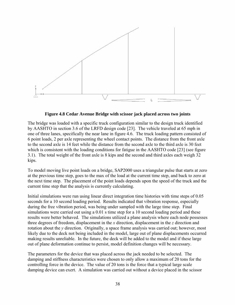
38

Figure 4.8 Cedar Avenue Bridge with scissor jack placed across two joints

The bridge was loaded with a specific truck configuration similar to the design truck identified by AASHTO in section 3.6 of the LRFD design code [23]. The vehicle traveled at 65 mph in one of three lanes, specifically the near lane in figure 4.6. The truck loading pattern consisted of 6 point loads, 2 per axle representing the wheel contact points. The distance from the front axle to the second axle is 14 feet while the distance from the second axle to the third axle is 30 feet which is consistent with the loading conditions for fatigue in the AASHTO code [23] (see figure 3.1). The total weight of the front axle is 8 kips and the second and third axles each weigh 32 kips.

To model moving live point loads on a bridge, SAP2000 uses a triangular pulse that starts at zero at the previous time step, goes to the max of the load at the current time step, and back to zero at the next time step. The placement of the point loads depends upon the speed of the truck and the current time step that the analysis is currently calculating.

Initial simulations were run using linear direct integration time histories with time steps of 0.05 seconds for a 10 second loading period. Results indicated that vibration response, especially during the free vibration period, was being under sampled with the large time step. Final simulations were carried out using a 0.01 s time step for a 10 second loading period and these results were better behaved. The simulations utilized a plane analysis where each node possesses three degrees of freedom, displacement in the x direction, displacement in the z direction and rotation about the y direction. Originally, a space frame analysis was carried out; however, most likely due to the deck not being included in the model, large out of plane displacements occurred making results unreliable. In the future, the deck will be added to the model and if these large out of plane deformation continue to persist, model definition changes will be necessary.

The parameters for the device that was placed across the jack needed to be selected. The damping and stiffness characteristics were chosen to only allow a maximum of 20 tons for the controlling force in the device. The value of 20 tons is the force that a typical large scale damping device can exert. A simulation was carried out without a device placed in the scissor

39

jack, and maximum displacements and velocities across the device were calculated. By equating the maximum force exerted by the device to 20 tons (40 kips), the stiffness constant k, for a pure linear stiffness element included in the scissor jack, was calculated to be 110 kips/in, and the damping constant c was determined to be 3 kips*s/in when a pure, linear damping element was placed in the scissor jack. This assured that the forces would not be larger than 40 kips and in reality, much less than 40 kips because displacements across the jack will be much smaller when a device with stiffness and damping is present. In fact, maximum forces actually exerted by the device were found to be only about 4 kips.

Multiple trials were run using different jack parameters and connections and the maximum positive and negative moments were calculated. The jack connections refer to how the jack is connected to the deck and can be either moment connections, as seen in figure 3.11, or truss connections, as seen in figure 3.13. Table 4.2 shows the results along with the overall reduction in moment range compared to the Cedar Avenue Bridge with no jack and an identical loading. The reason overall reduction in moment range is pertinent is because fatigue life is inversely proportional to the cube of the stress range [22]. It can be seen from table 4.2 that a higher magnification, m, leads to a higher moment range reduction. It can also be seen that the moment connection leads to larger reductions in moment range, but it should be noted that a rigid moment connection is more difficult to achieve than a truss connection in practice. If it is assumed that the moment range seen by the connection is proportional to the stress range, a 39% reduction in stress range leads to a 346% increase in fatigue life. Figure 4.9 shows the moment envelope for the scissor jack with a truss connection placed across two joints. Although it is difficult to discern in the figure, the moment ranges in each member within the jack have been reduced by almost 40%.

Table 4.2 Moment envelope at vulnerable joint on the Cedar Avenue Bridge with different scissor jack configurations

Trial Connection Type m k

(kip/in) c (kip*s/in)

Moment (kip-in) % reduction max min range

1 No jack - - 11654 -6827 18481 - 2 moment 30 0 0 11620 -6564 18184 1.61 3 moment 30 110 3 6811 -4412 11223 39.27 4 truss 30 0 0 11558 -6748 18306 0.95 5 truss 30 110 3 7669 -4792 12461 32.57 6 moment 15 0 0 11610 -6790 18400 0.44 7 moment 15 110 3 7346 -4524 11870 35.77 8 truss 15 0 0 11600 -6786 18386 0.51 9 truss 15 110 3 8434 -5145 13579 26.52

40

Figure 4.9 Moment range diagram for the Cedar Avenue Bridge with a scissor jack placed across the vulnerable region

4.4 Cedar Avenue Bridge Example Conclusions

The application of the response modification methodology on the Cedar Avenue Bridge example demonstrates the efficacy of the scissor jack device for reducing moment ranges seen by a connection or member in a bridge structure. By reducing the moment range, bridge life can be safely extended in structures with a finite fatigue life. Since the fatigue life is inversely proportional to the cube of the stress range, even small reductions in ranges can have a large effect on fatigue life. Assuming the connections in the Cedar Avenue Bridge had a finite fatigue life due to their stress concentrations, the scissor jack device could safely extend fatigue life by 346% giving bridge owners time to allocate funds to replace a bridge that has reached its design life limit.

41

Chapter 5: Summary and Conclusions

With a large number of bridges reaching the end of their intended design life, options for safe bridge life extension are becoming paramount for maintaining our infrastructure. Bridge health monitoring and structural response modification techniques are one possible mechanism for the safe extension of bridge life. To accomplish successful response modification, it is necessary to understand the four components addressed in this report: 1) common bridge vulnerabilities, 2) bridge loading models, 3) bridge monitoring systems, and 4) modification devices.

Due to the complexities of bridge failures, bridge vulnerabilities are not always easy to identify and classify. However, previous major bridge collapses have been reviewed and many common steel details with fatigue vulnerabilities have been identified as candidates for response modification and bridge health monitoring to safely extend bridge life. The mathematical concepts for the stress concentrations in cover plates and web gaps have been presented along with the equations for fatigue life adopted by AASHTO.

Bridge loading models can be defined in multiple ways. To extend bridge fatigue life, loading the bridge with an AASHTO specified truck is the most logical choice to allow for safe bridge life extension calculations. Because fatigue life is based on millions of loadings at a typical value, a standard truck loading is appropriate. Other models such as WIM are another possibility and would be helpful for bridges that see typical truck loads that are higher than the AASHTO specified truck.

The various applications of different bridge health monitoring systems have been categorized and useful systems have been identified. These systems can be used to analyze bridge responses to vehicle loading and verify that stress reduction has been achieved for safe life extension. Multiple systems will be necessary to provide both global bridge response measurements and local stress range readings. These systems can be linked to the control device and used for feedback control to allow for optimized stress range reduction at the vulnerable element.

Although many modification devices are currently deployed in earthquake applications, devices relevant to bridge health monitoring and structural response modification techniques have been identified. Passive, semi-active, and active devices can all be used in a bridge setting, but it seems that the best candidates are passive and semi-active devices due to their low or zero power consumption. These devices can be used to provide added stiffness and damping to allow for safe bridge life extension. Additional devices such as the scissor jack have been explored to allow for larger control forces by amplifying the typically small displacements seen in bridge applications. The mathematical relationships for the magnification of bridge displacements have been addressed and presented.

To successfully and safely extend the life of the bridge infrastructure, it is necessary to further extend the aforementioned principles and apply them to specific bridges and bridge vulnerabilities. The application of the response modification methodology on the Cedar Avenue Bridge demonstrates the efficacy of the scissor jack device for reducing moment ranges seen by a connection or member in a bridge structure. Due to the stress concentrations experienced by the connection detail, fatigue cracking is a major concern of the bridge owners. By reducing the moment range, bridge life can be safely extended in structures with a finite fatigue life. Since

42

the fatigue life is inversely proportional to the cube of the stress range, even small reductions in ranges can have a large effect on fatigue life. Assuming the connections in the Cedar Avenue Bridge had a finite fatigue life due to their stress concentrations, the scissor jack device could safely extend this life by 350% giving bridge owners time to allocate funds to replace a bridge that has reached its design life limit.

Response modification through scissor jack implementation has been successfully accomplished on the Cedar Avenue Bridge model. Future work should include adding the bridge deck to the Cedar Avenue Bridge model and carrying out a spatial analysis to confirm analysis results and refine the stress range calculations. Also, modeling response modification of bridges with other vulnerabilities such as cover plate and web gap distortion vulnerabilities is another potential demonstration of the value of response modification. Two potential modifications for these vulnerabilities are a device placed longitudinally across cover plates and a device installed laterally across diaphragm connections. Both would reduce deflection ranges (one in plane and one out of plane) and the associated stress ranges to help reduce the possibility of fatigue cracking. If stress ranges can be decreased on these details with stress category designations, fatigue life extension calculations can be carried out to quantify safe bridge life extension. A more detailed parameter study involving scissor jack configuration would also be helpful for determining ideal jack parameters.

In conclusion, bridge health monitoring and structural response modification techniques are a promising solution to address our aging bridge infrastructure in the United States. These techniques can reduce stress ranges at vulnerable bridge details by providing controlling forces along the member. By reducing and monitoring these stress ranges, bridge life extension can be accomplished in a safe and effective manner. Hopefully, it can also be shown that these techniques are not only viable as has been demonstrated in this report, but that they are also cost effective as well.

43

References

[1] Akesson, B. Understanding Bridge Collapses, Taylor and Francis, London, UK, 2008. [2] Fisher, J.W., Kaufmann, E.J., Wright, W., Xi, Z., Tjiang, H., Sivakumar, B., Edberg, W.

Hoan Bridge Forensic Investigation Failure Analysis, Final Report, Wisconsin Department of Transportation and FHWA, June 2001.

[3] Lichtenstein, A. “The Silver Bridge Collapse Recounted.” Journal of Performance of Constructed Facilities, Vol. 7, No. 4, November 1993. pp. 249-261.

[4] Richland Engineering Limited. Truss Gusset Plate Failure, Analysis, Repair and Retrofit: Interstate 90 Bridge over Grand River, Final Report, Mansfield, OH, April 1997.

[5] Hao, S. “I-35W Bridge Collapse.” Journal of Bridge Engineering, Vol. 15, No. 5, September/October 2010. pp. 608-614.

[6] Lindberg, A.Y., Schultz, A.E. Incorporation of Fatigue Detail Classification of Steel Bridges into the Minnesota Department of Transportation Database, Final Report 2007-22. Minnesota Department of Transportation, St. Paul, MN, June 2007.

[7] Thompson, D.J., Schultz, A.E. Development of an Advanced Structural Monitoring System, Final Report, University of Minnesota, Minneapolis, MN, September 2010.

[8] Enright, M.P., Frangopol, D.M. “Survey and Evaluation of Damaged Concrete Bridges.” Journal of Bridge Engineering, February 2000. pp. 31-38.

[9] O’Conner, J.S. “Bridge Safety Assurance Measures Taken in New York State.” Transportation Research Record, 1696, 2000. pp. 187-192.

[10] French C., Dexter, R., Altay, A. Effects of Increasing Truck Weight on Steel and Prestressed Bridges, Final Report 2003-16, Minnesota Department of Transportation, St. Paul, MN, May 2002.

[11] Nowak, A. “Bridge Live-Load Models.” Journal of Structural Engineering, Vol. 117, No. 9, September 1991. pp. 2757-2767.

[12] Nowak, A. “Bridge Load Models.” Proceedings of the 2003 ASCE/SEI Structures Congress and Exposition: Engineering Smarter, Seattle, WA, May 29-June 1, 2003.

[13] Miao, T.J., Chan, T.H.T. “Bridge Live Load Models from WIM Data.” Engineering Structures, Vol. 24, 2002. pp. 1071–1084.

[14] Patten, W.N., Sun, J., Li, G., Kuehn, J., Song, G. “Field Test of an Intelligent Stiffener for Bridges at the I-35 Walnut Creek Bridge.” Earthquake Engineering and Structural Dynamics, Vol. 28, No. 2, 1999. pp. 109-126.

[15] Christenson, R.E., Loebach, L.E. University of Connecticut, unpublished manuscript, private communication, 2009.

[16] Andrawes, B., DesRoches, R. “Unseating Prevention for Multiple Frame Bridges using Superelastic Devices.” Smart Materials and Structures, Vol. 14, 2005. pp. S60-S67.

[17] Cheng, F.Y., Jiang, H., Lou, K. Smart Structures, Innovative Systems for Seismic Response Control, CRC Press, Boca Raton, FL, 2008.

[18] Kim, J.M., Feng, M.Q., Shinozuka, M. “Energy Dissipating Restrainers for Highway Bridges.” Soil Dynamics and Earthquake Engineering, Vol. 19, 2000. pp. 65-69.

44

[19] Vukobratovic, M.K. “Active Structures in Advanced Engineering – An Overview.” International Journal of Computer Applications in Technology, Vol. 13, No. 1-2, 2000. pp. 10-24.

[20] Gastineau, A., Johnson, T., Schultz, A. Bridge Health Monitoring and Inspection Systems, Final Report, Minnesota Department of Transportation, St. Paul, MN, September 2009.

[21] Phares, B., Wipf, T., Greimann, L., Lee, Y. Health Monitoring of Bridge Structures and Components Using Smart Structure Technology, Wisconsin Highway Research Program Report, Vol. 1 and 2, Madison, WI, January 2005.

[22] Chotickai, P., Bowman, M. “Comparative Study of Fatigue Provisions for the AASHTO Fatigue Guide Specifications and LRFR Manual for Evaluation.” Journal of Bridge Engineering, Vol. 11, No. 5, September 2006. pp. 655-660.

[23] AASHTO. LRFD Bridge Design Specifications, 4th Ed., interim revisions, Washington D.C., 2009.

[24] Jajich, D., Schultz, A.E., Bergson, P.M., Galambos, T.V. Distortion-Induced Fatigue in Multi-Girder Steel Bridges, Final Report 2000-16, Minnesota Department of Transportation, St. Paul, MN, 2000.

[25] Berglund, E., Schultz, A.E. Analysis Tools and Rapid Screening Data for Assessing Distortional Fatigue in Steel Bridge Girders, Final Report 2002-06, Minnesota Department of Transportation, St. Paul, MN, 2002.

[26] Severtson, B., Beukema, F., Schultz, A.E. Rapid Assessment of Distortional Stresses in Multi Girder Steel Bridges, Final Report 2004-48, Minnesota Department of Transportation, St. Paul, MN, 2004.

[27] Li, H., Schultz, A.E. Rapid Assessment of Girder Differential Deflection and Distortional Fatigue Stress in Multi-Girder Steel Bridges, Final Report 2005-38, Minnesota Department of Transportation, St. Paul, MN, May 2005.

[28] Yang, G., Spencer, B., Carlson, J., Sain, M. “Large-scale MR fluid dampers: modeling and dynamic performance considerations.” Engineering Structures, Vol. 24, 2002. pp. 309-323.

[29] Sigaher, A., Constantinou, M. “Scissor-Jack-Damper Energy Dissipation System.” Earthquake Spectra, Vol. 19, No. 1, February 2003. pp. 133–158.

[30] Mathworks. Simulink 7 Reference. Accessed June 2010 http://www.mathworks.com/help/pdf_doc/simulink/slref.pdf.