response of micropiles in earth slopes from large …

RESPONSE OF MICROPILES IN EARTH SLOPES FROM LARGE-SCALE PHYSICAL MODEL TESTS

A Thesis Presented to the Faculty of the Graduate School University of Missouri-Columbia

In Partial Fulfillment Of the Requirements for the Degree

Master of Science

by ÖMER BOZOK

Dr. J. Erik Loehr, Thesis Supervisor

JULY 2009

The undersigned, appointed by the dean of the Graduate School, have examined the thesis

entitled

RESPONSE OF MICROPILES IN EARTH SLOPES FROM LARGE-SCALE PHYSICAL MODEL

TESTS

presented by Ömer Bozok,

a candidate for the degree of Master of Science in Civil Engineering,

and hereby certify that, in their opinion, it is worthy of acceptance.

Professor J. Erik Loehr, P.E.

Professor John Bowders, P.E.

Professor Michael Underwood

ii

Acknowledgements

It has been great pleasure for me to work with Dr. Loehr on this outstanding project. I

really appreciate the given opportunity. Dr. Loehr provided me everything that I asked for this

study to come true and he never minded setting up extra meetings in his already busy schedule.

His knowledge, diligence and innovativeness extended my desire to be a great engineer. I

consider myself one of the luckiest people to be his student. I would like to thank to Dr. Loehr for

not only providing me guidance throughout the research and in my coursework but also

expanding my academic vision.

I am sincerely thankful to Dr. Bowders for providing an enthusiasm to us, his students. It

has been a great honor to be one of his students. Projects that I have done for him not only

improved my ability to think critically but also improved my writing skill. I appreciate his concern

for student’s development. I am also grateful to Dr. Underwood for sparing his valuable time to

participate on my thesis committee and give me his valuable input.

I would like to thank Andrew Boeckmann and Nathan Textor, who worked on this

research previously for helping me when I needed assistance. Kyle Murphy, David Schone, John

Brightmann, Cory Ramsey and Wyatt Jenkins worked with me as undergraduate researchers and

performed every task I asked of them. I appreciate their friendship and would like to thank to each

of them for their willingness to help. I am thankful for Richard Coffman, Ryan Goetz, Daniel

Huaco, Amod Koirala, Tayler Day and Hamilton Puangnak who were also always willing to help. I

also appreciate the College of Engineering’s technical staff. This work would not have been

possible without Richard Oberto, Rex Gish, Rick Wells and Brian Samuels. And special thanks to

Dr. Peng Li. His study in numerical analysis helped this work to come true.

I would like to thank to National Science Foundation (Grant CMS 0093164) for providing

testing apparatus. I am also very grateful to Civil and Environmental Engineering Department for

providing me teaching assistantship.

Finally, I would like to thank my mother for her invaluable support and caring for me.

Without her support I would not be able to complete my studies.

iii

Table of Contents Acknowledgements............................................................................................ ii List of Tables ...................................................................................................... v List of Figures................................................................................................... vii Abstract ............................................................................................................ xxi Chapter 1: Introduction...................................................................................... 1

1.1 Background.........................................................................................................................1 1.2 Objectives & Methodology.................................................................................................3 1.3 Organization of Thesis .......................................................................................................4

Chapter 2: Literature Review............................................................................. 6 2.1 Micropiles ............................................................................................................................6 2.2 Design for Slopes Stabilized with Micropiles ..................................................................8

2.2.1 Loehr and Bowders (2003).........................................................................................9 2.2.2 Reese (1992)..............................................................................................................10 2.2.3 Isenhower (1999) ......................................................................................................11 2.2.4 FHWA Method ...........................................................................................................12

2.3 Limit Soil Pressure ...........................................................................................................14 2.4 Effect of Spacing on Resistance.....................................................................................15 2.5 Modeling in Geotechnical Engineering ..........................................................................16 2.6 Geotechnical Similitude in 1-g Physical Models ...........................................................18 2.7 Physical Modelling of Slopes Stabilized with Micropiles .............................................19

2.7.1 Deeken (2005)............................................................................................................20 2.7.2 Boeckmann (2006)....................................................................................................21 2.7.3 Textor (2007) .............................................................................................................22

2.8 Summary............................................................................................................................24 Chapter 3: Experimental Apparatus & Testing Procedure............................ 25

3.1 Model Container & Lifting Mechanism ...........................................................................25 3.2 Pore Pressure Control System........................................................................................28 3.3 Soil Properties...................................................................................................................29 3.4 Model Slope Geometry.....................................................................................................31 3.5 Model Reinforcement .......................................................................................................32 3.6 Instrumentation System...................................................................................................34

3.6.1 Pore Pressure Measurement...................................................................................34 3.6.2 Displacement Measurement ....................................................................................36 3.6.3 Strain Measurement & Data Reduction ..................................................................38 3.6.4 Kaolinite Marking Columns .....................................................................................45 3.6.5 Photographic Record of Test Progress .................................................................45

3.7 Testing Procedure ............................................................................................................46 3.7.1 Model Slope Construction .......................................................................................46 3.7.2 Reinforcing Member Installation.............................................................................48 3.7.3 Model Slope Testing.................................................................................................50 3.7.4 Forensic Evaluation .................................................................................................51

3.8 Summary............................................................................................................................52 Chapter 4: Testing Program & Results........................................................... 53

4.1 Testing Program ...............................................................................................................53 4.1.1 Test 3-D......................................................................................................................56 4.1.2 Test 3-E......................................................................................................................65 4.1.3 Test 3-F ......................................................................................................................75 4.1.4 Test 4-C......................................................................................................................84

4.2 Summary............................................................................................................................93

iv

Chapter 5: Analysis .......................................................................................... 94 5.1 Analysis Procedure ..........................................................................................................94 5.2 Results of Analyses for Individual Tests .....................................................................100

5.2.1 Results of Analyses for Tests in Group 1 ............................................................101 5.2.2 Results of Analyses for Tests in Group 2 ............................................................108 5.2.3 Results of Analyses for Tests in Group 3 ............................................................116 5.2.4 Results of Analyses for Tests in Group 4 ............................................................142

5.3 Summary..........................................................................................................................156 Chapter 6: Interpretation of Results ............................................................. 159

6.1 Effect of Pile Spacing .....................................................................................................159 6.2 Effect of Pile Batter Angle..............................................................................................164 6.3 Isolating Contributions to p- and y-multipliers............................................................165

6.3.1 “Model” Contribution, pm.......................................................................................167 6.3.2 First Approach Considering Spacing, Batter, and “Model” Contributions ......167 6.3.3 Second Approach...................................................................................................169 6.3.4 Contributions to y-multipliers ...............................................................................171

6.4 Recommended Method for Computing p- and y-multipliers......................................172 6.5 Methods for Estimating Limit Soil Pressure ................................................................172 6.6 Summary..........................................................................................................................175

Chapter 7: Summary, Conclusions & Recommendations .......................... 176 7.1 Summary..........................................................................................................................176 7.2 Conclusions ....................................................................................................................178 7.3 Recommendations..........................................................................................................180

References ...................................................................................................... 182 APPENDIX ....................................................................................................... 185

Test 1-A..................................................................................................................................186 Test 1-B..................................................................................................................................191 Test 1-C..................................................................................................................................198 Test 2-A..................................................................................................................................203 Test 2-B..................................................................................................................................211 Test 3-A..................................................................................................................................217 Test 3-B..................................................................................................................................226 Test 3-C..................................................................................................................................237 Test 3-D..................................................................................................................................248 Test 3-E ..................................................................................................................................259 Test 3-F ..................................................................................................................................270 Test 4-A..................................................................................................................................279 Test 4-B..................................................................................................................................286 Test 4-C..................................................................................................................................293

v

List of Tables

Table 2-1. Similitude for model tests in 1-g gravitational field (after Iai, 1989).............................19 Table 2-2. Summary of tests on models with stiff reinforcement by Deeken, 2005. ....................20 Table 2-3. Summary of tests on models with micropile reinforcement by Boeckmann, 2005. .....22 Table 2-4. Summary of tests on models with micropile reinforcement by Textor (2007). .............23 Table 3-1. Summary of results of index tests on model soil. ........................................................29 Table 3-2. Important quantities used to analyze strain gage data for upper bound

interprestations. ......................................................................................................................43 Table 3-3. Important quantities used to analyze strain gage data for lower bound interpretations.

................................................................................................................................................43 Table 4-1. Summary of testing parameters and results for each test. Test numbers with an

asterisk indicate tests reported by Boeckmann (2006) whereas test numbers with an apostrophe indicate tests reported by Textor (2007)..............................................................55

Table 5-1. Summary of tests in Group 1. .....................................................................................101 Table 5-2. Test parameters used for back-analyses of pile response for Test 1-A.....................101 Table 5-3. Back-calculated p- and y-multipliers for Test 1-A. ......................................................102 Table 5-4. Test parameters used for back-analyses of pile response for Test 1-B.....................104 Table 5-5. Back-calculated p- and y-multipliers for Test 1-B. ......................................................104 Table 5-6. Test parameters used for back-analyses of pile response for Test 1-C.....................106 Table 5-7. Back-calculated p- and y-multipliers for Test 1-C.......................................................106 Table 5-8. Summary of tests in Group 2. .....................................................................................108 Table 5-9. Test parameters used for back-analyses of pile response for Test 2-A.....................108 Table 5-10. Back-calculated p-, y- and t-multipliers for Test 2-A.................................................109 Table 5-11. Test parameters used for back-analyses of pile response for Test 2-B...................112 Table 5-12. Back-calculated p-, y- and t-multipliers for Test 2-B.................................................112 Table 5-13. Summary of Tests in Group 3. Test numbers with an asterisk indicate tests reported

by Boeckman (2006) whereas test numbers with an apostrophe indicate tests reported by Textor (2007). .......................................................................................................................116

Table 5-14. Test parameters used for back-analyses of pile response for Test 3-A...................117 Table 5-15. Back-calculated p-, y- and t-multipliers for Test 3-A.................................................117 Table 5-16. Test parameters used for back-analyses of pile response for Test 3-B...................121 Table 5-17. Back-calculated p-, y- and t-multipliers for Test 3-B.................................................121 Table 5-18. Test parameters used for back-analyses of pile response for Test 3-C...................125 Table 5-19. Back-calculated p-, y- and t-multipliers for Test 3-C. ...............................................125 Table 5-20. Test parameters used for back-analyses of pile response for Test 3-D...................129 Table 5-21. Back-calculated p-, y- and t-multipliers for Test 3-D. ...............................................129 Table 5-22. Test Parameters used for back-analyses of pile response for Test 3-E. .................133 Table 5-23. Back-calculated p-, y- and t-multipliers for Test 3-E.................................................133 Table 5-24. Test parameters used for back-analyses of pile response for Test 3-F. ..................138 Table 5-25. Back-calculated p-, y- and t-multipliers for Test 3-F.................................................138 Table 5-26. Summary of Tests in Group 4. Test numbers with an apostrophe indicate tests

reported by Textor (2007). ....................................................................................................142 Table 5-27. Test parameters used for back-analyses of pile response for Test 4-A...................143 Table 5-28. Back-calculated p-, y- and t-multipliers for Test 4-A.................................................143 Table 5-29. Test parameters used for back-analyses of pile response for Test 4-B...................147 Table 5-30. Back-calculated p-, y- and t-multipliers for Test 4-B.................................................147 Table 5-31. Test parameters used for back-analyses of pile response for Test 4-C...................152 Table 5-32. Back-calculated p-, y- and t-multipliers for Test 4-C. ...............................................152 Table 5-33. Summary of back-calculated p-, y- and t- multipliers for model tests.......................156 Table 6-1. Summary of back-calculated p- and y-multipliers for model tests. ............................166

vi

Table A 1. Summary of back-calculated p-, y- and t- multipliers for model tests.........................185 Table A 2. Test parameters used for back-analyses of pile response for Test 1-A.....................186 Table A 3. Back-calculated p- and y- multipliers for Test 1-A......................................................186 Table A 4. Test parameters used for back-analyses of pile response for Test 1-B.....................191 Table A 5. Back-calculated p- and y- multipliers for Test 1-B......................................................191 Table A 6. Test parameters used for back-analyses of pile response for Test 1-C. ...................198 Table A 7. Back-calculated p- and y- multipliers for Test 1-C......................................................198 Table A 8. Test parameters used for back-analyses of pile response for Test 2-A.....................203 Table A 9. Back-calculated p-, y- and t- multipliers for Test 2-A..................................................203 Table A 10. Test parameters used for back-analyses of pile response for Test 2-B...................211 Table A 11. Back-calculated p-, y- and t- multipliers for Test 2-B. ..............................................211 Table A 12. Test parameters used for back-analyses of pile response for Test 3-A...................217 Table A 13. Back-calculated p-, y- and t- multipliers for Test 3-A. ..............................................217 Table A 14. Test parameters used for back-analyses of pile response for Test 3-B...................226 Table A 15. Back-calculated p-, y- and t- multipliers for Test 3-B. ..............................................226 Table A 16. Test parameters used for back-analyses of pile response for Test 3-C. .................237 Table A 17. Back-calculated p-, y- and t- multipliers for Test 3-C. ..............................................237 Table A 18. Test parameters used for back-analyses of pile response for Test 3-D. .................248 Table A 19. Back-calculated p-, y- and t- multipliers for Test 3-D. ..............................................248 Table A 20. Test Parameters used for back-analyses of pile response for Test 3-E. .................259 Table A 21. Back-calculated p-, y- and t- multipliers for Test 3-E. ..............................................259 Table A 22. Test parameters used for back-analyses of pile response for Test 3-F. ..................270 Table A 23. Back-calculated p-, y- and t- multipliers for Test 3-F................................................270 Table A 24. Test parameters used for back-analyses of pile response for Test 4-A...................279 Table A 25. Back-calculated p-, y- and t- multipliers for Test 4-A. ..............................................279 Table A 26. Test parameters used for back-analyses of pile response for Test 4-B...................286 Table A 27. Back-calculated p-, y- and t- multipliers for Test 4-B. ..............................................286 Table A 28. Test parameters used for back-analyses of pile response for Test 4-C. .................293 Table A 29. Back-calculated p-, y- and t- multipliers for Test 4-C. ..............................................293

vii

List of Figures

Figure 1-1. Schematic of a slope stabilized with micropiles (from FHWA, 2005). ...........................2 Figure 2-1. Free body diagram for an individual slice where reinforcement intersects the sliding

surface. Note the reinforcement scheme shown is not a typical application of micropiles but rather some other type of in-situ reinforcement. The application of the limit equilibrium approach is the same for all types of in-situ reinforcement. .....................................................8

Figure 2-2. Schematic illustrating calculation of limit lateral resistance force for the method proposed by Loehr and Bowders (2003): (a) limit lateral soil pressure distribution and (b) location of equivalent resistance force. ..................................................................................10

Figure 2-3. Variation in limit soil pressure predicted by two common methods (from Parra, 2004).................................................................................................................................................15

Figure 2-4. Group efficiency for piles in a row (from Reese et al, 2006). .....................................16 Figure 2-5. Computed factors of safety as a function of slope angle for reinforced models (after

Deeken, 2005). .......................................................................................................................20 Figure 2-6. Schematic showing idealized lateral loading for stiff piles (from Deeken, 2005). ......21 Figure 3-1. Photograph of model container showing bottom drainage layer and Lexan® sheeting.

................................................................................................................................................26 Figure 3-2. Photograph of model container showing bottom grating after cleaning and before

replacing sand.........................................................................................................................26 Figure 3-3. Bracing system used to support the model container between tilting events. ...........27 Figure 3-4. Photograph of pore pressure control system. ............................................................28 Figure 3-5. Grain size distribution for the soil used in model slopes. ...........................................30 Figure 3-6. Proctor curves for the model soil. For both Proctor tests, specimens were

constructed in three lifts, and compaction was performed using a 5.5-lb hammer dropped from 12 in. Standard Proctor specimens were compacted with 25 blows per lift. Reduced Proctor specimens were compacted with 10 blows per lift. ....................................................30

Figure 3-7. Effective stress failure envelopes for model soil from direct shear tests. ..................31 Figure 3-8. Typical model slope geometries in (a) profile and (b) plan views. .............................32 Figure 3-9. SoilMoisture® tensiometer before installation. ...........................................................35 Figure 3-10. Tensiometer reservoirs mounted on the side of the model container. .....................36 Figure 3-11. Schematic representation of typical distribution of tensiometer tips within model

slopes......................................................................................................................................36 Figure 3-12. Deadman washer used to measure soil displacement.............................................37 Figure 3-13. Schematic showing typical distribution of displacement gages within models.........37 Figure 3-14. String potentiometer in protective housing. ..............................................................38 Figure 3-15. Strain gages are attached to a clean surface using strain gage glue. Inset shows

close view of attached strain gage. ........................................................................................39 Figure 3-16. Four-point bending tests used to calibrate strain gages. .........................................40 Figure 3-17. Analysis conditions for strain gage data: (a) upper bound interpretation, (b)

intermediate interpretation, (c) lower bound interpretation.....................................................41 Figure 3-18. Kaolinite marking column exposed during deconstruction. Break in the column is

interpreted as the failure surface. ...........................................................................................45 Figure 3-19. Example photograph recorded by overhead network camera. ................................46 Figure 3-20. Photographs of the model construction process: (a) tilling soil, (b) placing loose soil,

(c) spreading soil into lifts, and (d) compacting soil with smooth drum roller. ........................47 Figure 3-21. Model slope at end of construction. Model shown was built with a capping beam,

shown in the middle of the slope. ...........................................................................................48 Figure 3-22. Reinforcing member installation process: (a) drilling hole, (b) checking hole

inclination and length, (c) partially filling hole with grout, and (d) inserting steel pipe while vibrating to remove air voids in grout......................................................................................49

Figure 3-23. (a) Auger used to install model micropiles. (b) Photograph of model pile exhumed following test completion.........................................................................................................49

viii

Figure 3-24. Photograph of the model container after initial tilting during testing.........................50 Figure 3-25. Example of a vertical cut exposed during forensic investigation..............................51 Figure 4-1. Schematic drawings showing model reinforcement arrangements: (a) Group 1 - tests

with single row of micropiles perpendicular to slope; (b) Group 2 – tests with micropiles battered at ±30° from perpendicular without a capping beam; (c) Group 3 - tests with micropiles battered at ±30° from perpendicular with a capping beam; (d) Group 4 - tests with micropiles battered at ±15° from perpendicular with a capping beam. Drawings are not to scale........................................................................................................................................54

Figure 4-2. Model 3-D during test. ................................................................................................56 Figure 4-3. Inclination in time history for Test 3-D. .......................................................................57 Figure 4-4. Instrumentation placement for Test 3-D: (a) wireline extensometers; (b) tensiometers;

and (c) strain gages. Numerals indicate gage numbers and centers of circles are the gage locations..................................................................................................................................58

Figure 4-5. Failure of Model 3-D: (a) no apparent crack on model; (b) tension cracks propagate across crest while toe fails; (c) cracks widen as model deforms; (d) soil flows through micropiles................................................................................................................................59

Figure 4-6. Model 3-D after failure. ...............................................................................................60 Figure 4-7. Observed failure surface for Model 3-D. ....................................................................60 Figure 4-8. Total soil movement records for Test 3-D. Numerals next to line indicate the gage

number. Numbers at top indicate the slope inclinations.........................................................61 Figure 4-9. Pore pressure records for Test 3-D. Numerals next to lines indicate gage number.

Numbers at top indicate the slope inclinations. ......................................................................62 Figure 4-10. Mobilized loads in Member 2 (inclined downslope) from Test 3-D at slope inclination

of 46º: (a) bending moment; (b) axial force. ...........................................................................64 Figure 4-11. Mobilized loads in Member 3 (inclined upslope) from Test 3-D at slope inclination of

46º: (a) bending moment; (b) axial force. ...............................................................................64 Figure 4-12. Model 3-E during test. ...............................................................................................65 Figure 4-13. Inclination history for Test 3-E. ..................................................................................66 Figure 4-14. Instrumentation scheme for Test 3-E: (a) wireline extensometers; (b) tensiometers;

and (c) strain gages. Numerals indicate gage numbers, and circles indicate gage locations.................................................................................................................................................67

Figure 4-15. Failure of Model 3-E: (a) no apparent cracks on model; (b) toe failure that occurred at slope inclination of 45 degrees; (c) soil flowing through members on left side of model; (d) overall failure at slope inclination of 47 degrees.....................................................................68

Figure 4-16. Observed failure surface for Model 3-E.....................................................................69 Figure 4-17. Model 3-E after toe failure at slope inclination of 45 degrees. ..................................70 Figure 4-18. Model 3-E after overall failure....................................................................................70 Figure 4-19. Total soil movement records for Test 3-E. Numerals next to line indicate the gage

number. Numbers at top indicate the slope inclinations.........................................................71 Figure 4-20. Pore pressure records for Test 3-E. Numerals next to line indicates gage number.

Numbers at top indicate the slope inclinations. ......................................................................72 Figure 4-21. Mobilized loads in Member 2 (inclined downslope) from Test 3-E at slope inclination

of 45º: (a) bending moment; (b) axial force. ...........................................................................74 Figure 4-22. Mobilized loads in Member 3 (inclined upslope) from Test 3-E at slope inclination of

45º: (a) bending moment; (b) axial force. ...............................................................................74 Figure 4-23. Inclination history for Test 3-F. ..................................................................................75 Figure 4-24. Instrumentation scheme for Test 3-F: (a) wireline extensometers; (b) tensiometers;


Figure 4-25. Failure of Model 3-F: (a) no apparent cracks on model; (b) toe failure that occurred at slope inclination of 40 degrees; (c) failure of slope above capping beam; (d) overall failure that occurred at slope inclination of 46 degrees. ....................................................................78

Figure 4-26. Model 3-F after overall failure....................................................................................79 Figure 4-27. Observed failure surface for Model 3-F.....................................................................79 Figure 4-28. Total soil movement records for Test 3-F. Numerals next to lines indicate the gage

number. Numbers at top indicate the slope inclinations.........................................................80

ix

Figure 4-29. Pore pressure records for Test 3-F. Numerals next to line indicates gage number. Numbers at top indicate the slope inclinations. ......................................................................81

Figure 4-30. Mobilized loads in Member 1 (inclined downslope) from Test 3-F at slope inclination of 45º: (a) bending moment; (b) axial force. ...........................................................................83

Figure 4-31. Mobilized loads in Member 3 (inclined upslope) from Test 3-F at slope inclination of 45º: (a) bending moment; (b) axial force. ...............................................................................83

Figure 4-32. Model 4-C during test. ...............................................................................................84 Figure 4-33. Inclination history for Test 4-C...................................................................................85 Figure 4-34. Instrumentation scheme for Test 4-C: (a) wireline extensometers; (b) tensiometers;


Figure 4-35. Failure of Model 4-C: (a) no apparent cracks on model; (b) toe failure that occurred at a slope inclination of 48 degrees; (c) cracks forming above the capping beam; (d) overall failure of model at slope inclination of 48 degrees. ................................................................87

Figure 4-36. Photograph of Model 4-C after failure at 48 degrees. ...............................................88 Figure 4-37. Observed failure surface for Model 4-C. ...................................................................88 Figure 4-38. Total soil movement records for Test 4-C. Numerals next to line indicate the gage

number. Numbers at top indicate the slope inclinations.........................................................89 Figure 4-39. Pore pressure records for Test 4-C. Numerals next to line indicates gage number.

Numbers at top indicate the slope inclinations. ......................................................................90 Figure 4-40. Mobilized loads in Member 2 (inclined downslope) from Test 4-C at slope inclination

of 46º: (a) bending moment; (b) axial force. ...........................................................................92 Figure 4-41. Mobilized loads in Member 1 (inclined upslope) from Test 4-C at slope inclination of

46º: (a) bending moment; (b) axial force. ...............................................................................92 Figure 5-1. Example of soil movement profiles used for analyses of pile response to moving soil

(from Test 3-A). Numbers in legend indicate slope inclination. ..............................................95 Figure 5-2. p-y curves for Reese sand model with p- and y-multipliers.........................................97 Figure 5-3. Effect of p-multiplier on the limit soil pressure of the Reese sand model. Profiles

indicate the limit resistance at a given depth (- = pile pushing upslope). ...............................97 Figure 5-4. Effect of t-multiplier on elastic-perfectly plastic t-z model. ..........................................98 Figure 5-5. Comparisons of measured and predicted response for Member 2 from Test 1-A when

inclined at 40°: (a) bending moment (+ = tension upslope); (b) shear force (- = pushing upslope); (c) net soil pressure (- = pushing upslope). For legend, number in parentheses indicates magnitude of soil movement in inches. .................................................................103

Figure 5-6. Comparisons of measured and predicted response for Member 3 from Test 1-B when inclined at 42°: (a) bending moment (+ = tension upslope); (b) shear force (- = pushing upslope); (c) net soil pressure (- = pushing upslope). For legend, number in parentheses indicates magnitude of soil movement in inches. .................................................................105

Figure 5-7. Comparisons of measured and predicted response for Member 3 from Test 1-C when inclined at 44°: (a) bending moment (+ = tension upslope); (b) shear force (- = pushing upslope); (c) net soil pressure (- = pushing upslope). For legend, number in parentheses indicates magnitude of soil movement in inches. .................................................................107

Figure 5-8. Comparisons of measured and predicted response for Member 2 from Test 2-A when inclined at 44°: (a) bending moment (+ = tension upslope); (b) shear force (- = pushing upslope); (c) net soil pressure (- = pushing upslope); (d) axial force (+ = tension). For legend, number in parentheses indicates magnitude of soil movement in inches. ...........................110


Figure 5-10. Comparisons of measured and predicted response for Member 2 from Test 2-B when inclined at 42°: (a) bending moment (+ = tension upslope); (b) shear force (- = pushing upslope); (c) net soil pressure (- = pushing upslope); (d) axial force (+ = tension). For legend, number in parentheses indicates magnitude of soil movement in inches. ...........................113

x






Figure 5-16. Comparisons of measured and predicted response for Member 3 from Test 3-C when inclined at 43°: (a) bending moment (+ = tension upslope); (b) shear force (- = pushing upslope); (c) net soil pressure (- = pushing upslope); (d) axial force (+ = tension). For legend, number in parentheses indicates magnitude of soil movement in inches. ...........................127

Figure 5-17. Comparisons of measured and predicted response for Member 2 from Test 3-C when inclined at 42°: (a) bending moment (+ = tension upslope); (b) shear force (- = pushing upslope); (c) net soil pressure (- = pushing upslope); (d) axial force (+ = tension). For legend, number in parentheses indicates magnitude of soil movement in inches. ...........................128

Figure 5-18. Comparisons of measured and predicted response for upslope members from Test 3-D when inclined at 46°: (a) bending moment (+ = tension upslope); (b) shear force (- = pushing upslope); (c) net soil pressure (- = pushing upslope); (d) axial force (+ = tension). For legend, number in parentheses indicates magnitude of soil movement in inches. Horizontal bars indicate upper and lower bound for Member 3............................................131

Figure 5-19. Comparisons of measured and predicted response for downslope members from Test 3-D when inclined at 46°: (a) bending moment (+ = tension upslope); (b) shear force (- = pushing upslope); (c) net soil pressure (- = pushing upslope); (d) axial force (+ = tension). For legend, number in parentheses indicates magnitude of soil movement in inches. Horizontal bars indicate upper and lower bound for Member 2............................................132

Figure 5-20. Comparisons of measured and predicted response for upslope members from Test 3-E when inclined at 45°: (a) bending moment (+ = tension upslope); (b) shear force (- = pushing upslope); (c) net soil pressure (- = pushing upslope); (d) axial force (+ = tension). For legend, number in parentheses indicates magnitude of soil movement in inches. Horizontal bars indicate upper and lower bound for Member 3............................................135

Figure 5-21. Comparisons of measured and predicted response for upslope members from Test 3-E when inclined at 43°: (a) bending moment (+ = tension upslope); (b) shear force (- = pushing upslope); (c) net soil pressure (- = pushing upslope); (d) axial force (+ = tension). For legend, number in parentheses indicates magnitude of soil movement in inches. Horizontal bars indicate upper and lower bound for Member 3............................................136

Figure 5-22. Comparisons of measured and predicted response for downslope members from Test 3-E when inclined at 45°: (a) bending moment (+ = tension upslope); (b) shear force (- = pushing upslope); (c) net soil pressure (- = pushing upslope); (d) axial force (+ = tension). For legend, number in parentheses indicates magnitude of soil movement in inches. Horizontal bars indicate upper and lower bound for Member 2............................................137

xi

Figure 5-23. Comparisons of measured and predicted response for upslope members from Test 3-F when inclined at 45°: (a) bending moment (+ = tension upslope); (b) shear force (- = pushing upslope); (c) net soil pressure (- = pushing upslope); (d) axial force (+ = tension). For legend, number in parentheses indicates magnitude of soil movement in inches. Horizontal bars indicate upper and lower bound for Member 3............................................140

Figure 5-24. Comparisons of measured and predicted response for downslope members from Test 3-F when inclined at 45°: (a) bending moment (+ = tension upslope); (b) shear force (- = pushing upslope); (c) net soil pressure (- = pushing upslope); (d) axial force (+ = tension). For legend, number in parentheses indicates magnitude of soil movement in inches. Horizontal bars indicate upper and lower bound for Member 1............................................141






Figure 5-30. Comparisons of measured and predicted response for upslope members from Test 4-C when inclined at 47°: (a) bending moment (+ = tension upslope); (b) shear force (- = pushing upslope); (c) net soil pressure (- = pushing upslope); (d) axial force (+ = tension). For legend, number in parentheses indicates magnitude of soil movement in inches. Horizontal bars indicate upper and lower bound for Member 1............................................154

Figure 5-31. Comparisons of measured and predicted response for downslope members from Test 4-C when inclined at 47°: (a) bending moment (+ = tension upslope); (b) shear force (- = pushing upslope); (c) net soil pressure (- = pushing upslope); (d) axial force (+ = tension). For legend, number in parentheses indicates magnitude of soil movement in inches. Horizontal bars indicate upper and lower bound for Member 2............................................155

Figure 6-1. Back-calculated p-multipliers vs. pile spacing ratio for (a) upslope piles, and (b) downslope piles. ...................................................................................................................160

Figure 6-2. Back-calculated y-multiplier vs. spacing ratio. Data are from tests where piles were installed through a capping beam. Numbers in legend indicate batter angle (negative sign for upslope pile)..........................................................................................................................161

Figure 6-3. Schematic drawing of models prepared by Goh et al., (2008). Piles (5/8in diameter) were installed vertically into (12in x 12in) container with pinned head and tip condition, (a) spacing ratio of 3, soil flow around the piles (b) spacing ratio of 6, soil flow through and around the piles. Numbers next to piles indicate the mobilized resistance compared to single pile. Drawings are not to scale.............................................................................................162

Figure 6-4. Schematic drawing of models prepared in this study. Soil flows through the piles. Drawing is not to scale..........................................................................................................162

Figure 6-5. Combined effect of capping beam, pile spacing and batter angle on pile response vs. pile spacing. ..........................................................................................................................163

Figure 6-6. Back-calculated p-multipliers vs. batter angle for various spacing ratios..................164

xii

Figure 6-7. Effect of batter angle on soil resistance and trend recommended by Reese et al. 2006. .....................................................................................................................................165

Figure 6-8. Computed batter multiplier, pb, vs. batter angle established for tests with pile spacing ratios greater than 9, assuming pm = 0.5 and ps = 1.0 . Positive batter for downslope pile. .168

Figure 6-9. Spacing multiplier, ps, established assuming that pm = 0.5 and pb taken from Figure 6-8, vs. spacing ratio.............................................................................................................169

Figure 6-10. Batter multiplier, pb, vs. batter angle for second approach......................................170 Figure 6-11.Cap multiplier, pc, vs. spacing ratio for second approach. .......................................170 Figure 6-12. y-multiplier vs. spacing ratio. Numbers next to trends indicate the batter angle. Solid

lines are for piles with the capping beam while dashed lines are for piles without the capping beam. ....................................................................................................................................171

Figure 6-13. Scaled limit soil pressure prediction of methods vs. prediction from pile response analysis for piles battered 30° (a) upslope pile; (b) downslope pile. ....................................174

Figure 6-14. Distribution of mobilized load along the full length of pile just prior to failure. Data belongs the Test 1-A. Profile of limit soil pressure is obtained by extending the trend that increases quasi-linearly with depth (the dashed line in the figure).......................................175

Figure A 1. Comparisons of measured and predicted response for Member 2 from Test 1-A when

inclined at 30°: (a) bending moment (+ = tension upslope); (b) shear force (- = pushing upslope); (c) net soil pressure (- = pushing upslope). For legend, number in parentheses indicates magnitude of soil movement in inches. .................................................................187

Figure A 2. Comparisons of measured and predicted response for Member 2 from Test 1-A when inclined at 35°: (a) bending moment (+ = tension upslope); (b) shear force (- = pushing upslope); (c) net soil pressure (- = pushing upslope). For legend, number in parentheses indicates magnitude of soil movement in inches. .................................................................188



Figure A 5. Comparisons of measured and predicted response for Member 3 from Test 1-B when inclined at 30°: (a) bending moment (+ = tension upslope); (b) shear force (- = pushing upslope); (c) net soil pressure (- = pushing upslope). For legend, number in parentheses indicates magnitude of soil movement in inches. .................................................................192





xiii


Figure A 11. Comparisons of measured and predicted response for Member 3 from Test 1-C when inclined at 34°: (a) bending moment (+ = tension upslope); (b) shear force (- = pushing upslope); (c) net soil pressure (- = pushing upslope). For legend, number in parentheses indicates magnitude of soil movement in inches. .................................................................199













xiv















xv















xvi




Figure A 55. Comparisons of measured and predicted response for upslope piles from Test 3-D when inclined at 30°: (a) bending moment (+ = tension upslope); (b) shear force (- = pushing upslope); (c) net soil pressure (- = pushing upslope). For legend, number in parentheses indicates magnitude of soil movement in inches. Horizontal bars indicate upper and lower bound for Member 3. ............................................................................................................249





Figure A 60. Comparisons of measured and predicted response for downslope piles from Test 3-D when inclined at 30°: (a) bending moment (+ = tension upslope); (b) shear force (- = pushing upslope); (c) net soil pressure (- = pushing upslope). For legend, number in parentheses indicates magnitude of soil movement in inches. Horizontal bars indicate upper and lower bound for Member 2.............................................................................................254



xvii



Figure A 65. Comparisons of measured and predicted response for upslope piles from Test 3-E when inclined at 36°: (a) bending moment (+ = tension upslope); (b) shear force (- = pushing upslope); (c) net soil pressure (- = pushing upslope). For legend, number in parentheses indicates magnitude of soil movement in inches. Horizontal bars indicate upper and lower bound for Member 3. ............................................................................................................260





Figure A 70. Comparisons of measured and predicted response for downslope piles from Test 3-E when inclined at 36°: (a) bending moment (+ = tension upslope); (b) shear force (- = pushing upslope); (c) net soil pressure (- = pushing upslope). For legend, number in parentheses indicates magnitude of soil movement in inches. Horizontal bars indicate upper and lower bound for Member 2.............................................................................................265




xviii


Figure A 75. Comparisons of measured and predicted response for upslope piles from Test 3-F when inclined at 34°: (a) bending moment (+ = tension upslope); (b) shear force (- = pushing upslope); (c) net soil pressure (- = pushing upslope). For legend, number in parentheses indicates magnitude of soil movement in inches. Horizontal bars indicate upper and lower bound for Member 3. ............................................................................................................271




Figure A 79. Comparisons of measured and predicted response for downslope piles from Test 3-F when inclined at 34°: (a) bending moment (+ = tension upslope); (b) shear force (- = pushing upslope); (c) net soil pressure (- = pushing upslope). For legend, number in parentheses indicates magnitude of soil movement in inches. Horizontal bars indicate upper and lower bound for Member 1.............................................................................................275






xix











Figure A 95. Comparisons of measured and predicted response for upslope piles from Test 4-C when inclined at 30°: (a) bending moment (+ = tension upslope); (b) shear force (- = pushing upslope); (c) net soil pressure (- = pushing upslope). For legend, number in parentheses indicates magnitude of soil movement in inches. Horizontal bars indicate upper and lower bound for Member 1. ............................................................................................................294



xx



Figure A 100. Comparisons of measured and predicted response for downslope piles from Test 4-C when inclined at 30°: (a) bending moment (+ = tension upslope); (b) shear force (- = pushing upslope); (c) net soil pressure (- = pushing upslope). For legend, number in parentheses indicates magnitude of soil movement in inches. Horizontal bars indicate upper and lower bound for Member 2.............................................................................................299





xxi

Abstract

Slope failures can arise from many factors and of such failures can have a big impact on

public and private infrastructure. Micropiling is a relatively new approach in slope stabilization

applications that has been adopted by many agencies and used in many problematic sites across

the globe. However, limited knowledge reggarding load transfer for piles within moving soil may

cause design of micropiles to be more conservative than is actually needed. The objective of the

research presented is to provide needed experimental data to improve prediction of limit loads for

micropiles in slope stabilization applications. More specifically, the objective is to provide

guidance on the effects of pile batter and spacing so designers can reasonably account for these

effects when predicting the limit resistance values for micropiles.

Experimental data was obtained from tests of large-scale physical models of slopes

stabilized with micropiles. The experimental apparatus includes a model container, a pore

pressure/soil movement control system, model reinforcement, and an instrumentation system.

The container accommodates model slopes that are up to 7.4 ft by 14 ft in plan view with slope

heights of up to 5 ft. This scale is large enough to permit construction of model slopes and

associated stabilization schemes using techniques that closely mimic common field procedures,

thereby reducing issues with scale effects that are commonly encountered with smaller scale

models. The reinforcement consisted of 1.5 and 2.0-in. diameter gravity-grouted micropiles

reinforced with 0.75-in. and 1.25-in. diameter steel pipe with 0.095-in. wall thickness. The

reinforcement was designed so that its flexural stiffness was appropriately scaled down from a

common flexural stiffness values for full-scale micropiles. Instrumentation utilized included

tensiometers for monitoring pore water pressures (or suctions), wire-line extensometers for

monitoring soil movement within the model slopes, as well as strain gages to monitor loads in the

micropiles.

The testing program includes fourteen tests, including those reported by Boeckmann

(2006) and Textor (2007). These tests were divided into four different groups. For the first group

of tests, three tests were performed using models with micropiles installed perpendicular to the

xxii

slope face. The second group of tests included two models with micropiles installed in an A-

frame arrangement with piles installed 30 degrees upslope and downslope of the line

perpendicular to the slope face. For the third group, six tests were performed using models with

micropiles installed in an A-frame arrangement through a capping beam with piles alternating

between 30 degrees upslope and 30 degrees downslope of the perpendicular to the slope face.

For the final group, three tests were performed using models prepared in a similar manner to

models these in Group 3, except that the piles were battered at 15 degrees from the perpedicular.

Within each group of tests, member spacing was varied to evaluate its effect in addition to that of

member inclination and member size. Pore pressures, soil movement, and loads in the

micropiles were monitored and recorded throughout each test.

Load transfer to the model piles within the moving soil mass was analyzed using soil-

structure interaction methods. Based on measured soil movements and sliding surface locations,

p-y and t-z analyses were performed to back-calculate “best fit” p-; y-; and t-multipliers that would

lead to prediction of the measured bending moments and axial loads in the model micropiles. The

back-calculated p-y and t-z parameters were compared with values from literature and with one

another to develop recommendations for predicting axial and lateral resistance in micropiles for

slope stabilization applications.

As a result of this study, a method was established to obtain p- and y-multipliers for any

combination of spacing and batter angle, both with and with out capping beam. Results of

analysis indicate that spacing ratio and batter angle are important factors that influence the limit

soil pressure/resistance. Data suggests that closer spacing increases the limit soil pressure, but

batter angle was observed to have the greatest effect on limit soil pressure. Data shows that

available resistance increases with batter angle from the lower values for piles inclined upslope to

the greater values for piles inclined downslope. No clear trend was observed among

spacing/batter and maximum bending moment for the tests due to changes in the location of

sliding surface for each pile and for each test. The effect of pile diameter was observed to be

limited within the scatter of data for the small range of diameters considered in this work.

1

Chapter 1:Introduction

1.1 Background Slope failures and landslides cause significant hazards to all types of both public and

private infrastructure. The Transportation Research Board has reported that direct costs for

maintenance and repair of landslides involving U.S highways exceed about $100 million annually

(Transportation Research Board, 1996). There are many ways to deal with problematic slopes.

One way is to increase the stability of slope by micropiling, which is relatively new approach.

Micropiles (also known as minipiles, pin piles, root piles, pali radice, and a series of other names)

are small diameter drilled and grouted in-situ reinforcement as shown in Figure 1-1.1. The

approach is based on techniques developed in the 1950’s for underpinning of historic structures

in Europe (Lizzi, 1982). Micropiles may or may not include steel reinforcing bars or pipes and may

be installed with distributed spacing or in closely spaced groups or networks to form a three-

dimensional, “reticulated” structure. Use of micropiles for slope stabilization is similar to the

practice of “soil doweling” in which large piles or drilled shafts are installed in a single row, or

occasionally multiple rows, to stabilize a slope (Bruce and Juran, 1997). However, micropiles

differ from soil dowels in that they have significantly lower bending resistance and therefore

transfer load in a combination of tension, bending, and shear (Bruce and Juran, 1997).

2

Figure 1-1. Schematic of a slope stabilized with micropiles (from FHWA, 2005).

Micropiles have been successfully used for stabilization of many problematic slopes in

the U.S. and abroad (e.g. Pearlman et al., 1992; Brown and Wolosick, 1995; Guilloux and

Schlosser, 1982; Turner et al., 1998). Their effectiveness on slope stabilization is therefore

apparent. However, this technique has not been adopted widely due to two reasons: (1) limited

knowledge and data on the development of forces within reinforcing members and (2) a lack of

fundamental understanding of the interaction between the soil and reinforcing members (Bruce

and Juran, 1997). Therefore, designs are generally conservative out of necessity, which often

produces uneconomical solutions when compared to other potential stabilization methods.

There is general agreement in the literature (e.g. Bruce and Juran, 1997; Pearlman et al.,

1992; Brown and Wolosick, 1995; Chen and Poulos, 1997; Parra et al., 2004) that the current

state of knowledge in the area of slope stabilization with piling is limited by:

3

Lack of understanding of interaction among closely spaced reinforcing members and

the surrounding soil;

Lack of accurate measurements to determine the mobilization of forces within

reinforcing elements during loading of the piles;

Lack of knowledge of the limiting soil pressures; and

Lack of knowledge on optimum geometric arrangements for in-situ reinforcing

members;

Reducing these uncertainties would most likely make the application of micropiles more

economical for slope stabilization applications.

1.2 Objectives & Methodology The uncertainties mentioned in the previous section may lead to uneconomical design. The

main objective of this study is to provide guidance on the effects of pile spacing and pile batter

when predicting loads in micropiles for slope stabilization. This includes developing better

estimates of limit soil pressure and a better understanding of the load transfer process between

moving soil and micropiles. Specifically, a better understanding of the load transfer process

includes knowledge of the effects of member spacing, batter angle, and pile diameter.

The method adopted to achieve these objectives is to test large-scale physical models of

slopes stabilized with micropiles at different pile spacing ratios, batter angles, and arrangements.

The models were built in a large-scale landslide simulator that has several distinct advantages

over other related techniques such as centrifuge modeling and full-scale field testing. The basic

principle behind the device is to induce failure by incrementally increasing the slope angle to the

point of failure. By doing so, it is possible to load the model slope up to and including failure

without the consequences and complexities present in performing full-scale field tests. Loading

can also be controlled more precisely than in field applications and instrumentation can be more

reliably monitored and maintained in a controlled laboratory environment. The apparatus used is

capable of modeling much larger models than is possible with the largest geotechnical

centrifuges available at this time. In doing so, difficulties with scaling down soil particles and soil-

reinforcement interface features are diminished (of particular importance for in-situ reinforcement

4

applications since the interaction between the soil and reinforcing elements and among

reinforcing elements is likely scale dependent). Preparation of soil "samples" and model

reinforcing elements mimic field construction processes more closely than is possible with the

centrifuge, and the large size of the tilt apparatus limits the influence of boundary effects. While

tilt loading does not precisely model field conditions (no model test ever does), it enables a large

amount of valuable data to be obtained at a relatively rapid rate.

The large-scale landslide simulator was used to test fourteen models for this research.

Three of these models contained micropiles installed perpendicular to slope face without a

capping beam. Two contained micropiles in an A-frame arrangement installed without a capping

beam. Nine models contained micropiles in an A-frame arrangement installed through a capping

beam that fixes the heads of the micropiles to one another. Each model was instrumented to

measure pore pressures, soil movement, and loads induced in the micropiles. Additional

instrumentation was used to identify the location of the failure surface and to record photographs

of the failure process. After collecting and analyzing the data, p-y and t-z analyses were

performed to match the load transfer data measured during each test with predictions produced in

the analyses. The resulting “back-calculated” parameters for each model were then analyzed to

evaluate the effects of member spacing, batter angle, and pile diameter. They were also

compared with values reported in literature. The results of all tests and analyses are reported in

this thesis.

1.3 Organization of Thesis This thesis is organized into seven chapters. A review of pertinent literature is presented in

Chapter 2. This begins with a general description of micropiles, followed by a summary of current

design methods for slopes with in-situ reinforcement and methods for predicting the limit soil

pressure. Geotechnical engineering modeling topics are then presented, including comparisons

of 1-g physical modeling with centrifuge modeling and full-scale field testing. A discussion of

similitude follows. Lastly, a summary of previous work on physical modeling of micropiles is

presented. This includes previous work performed using the large-scale landslide simulator.

5

A description of the experimental apparatus is presented in Chapter 3. The apparatus

consists of a model container, a pore pressure control system, model reinforcement, and an

instrumentation system to measure pore pressure, soil movement, and loading of the micropiles.

Chapter 3 also contains a summary procedures used for each test, from construction through

forensic evaluation.

The testing program is described and experimental results are presented in Chapter 4.

The description explains how the fourteen tests were divided among four groups depending on

the member inclination and whether a capping beam was used. Results for each test, including

details about model construction and failure, instrumentation, records of pore pressure and soil

movement, and micropile loading, are also presented.

Data analysis procedures and results are presented in Chapter 5. Methods for back-

calculating parameters to match the measured data are explained before presenting the results of

analyses for instrumented micropiles. In Chapter 6, the back-calculated parameters are then

compared with values from literature and one another to evaluate load transfer to the micropiles.

Finally, a summary of this thesis, conclusions based on the results of this work, and

recommendations for the design of micropiles and future work are presented in Chapter 7.

6

Chapter 2:Literature Review

In this chapter, the history, applications, and classification of micropiles are summarized.

This is followed by explanation of existing design methods related to slope stabilization with in-

situ reinforcement. Several limit soil pressure theories are then presented. Next, 1-g physical

modeling is compared with centrifuge modeling and full-scale field testing for geotechnical

engineering applications. An overview of important similitude considerations for 1-g physical

modeling of geotechnical applications is then presented. Finally, previous work on physical

modeling of micropiles are summarized, including tests performed using the apparatus used for

the work described in this thesis.

2.1 Micropiles Micropiles are small-diameter piles that are drilled and grouted and typically reinforced

with steel. Usually, the diameter of a micropile is less than 12 in. (FHWA, 2005). Steel

reinforcement in a micropile often occupies a greater percentage (up to one half) of the shaft

volume than is common for other cast-in-place piles (FHWA, 2005). Micropiles can resist axial

and/or lateral loads. The ground-grout bond value for micropiles is often high as a result of

grouting and installation procedures. Because of the high friction and small bearing area of a

micropile, end bearing is often ignored.

Micropiles can be installed in any ground condition, requiring only minimal site access

and headroom which makes micropiles efficient in low head conditions. Also, micropiles are

installed with minimal disturbance to surrounding structures. These advantages make micropiles

particularly well-suited for underpinning existing structures. Indeed, this is the historical

application that resulted in the development of the micropile by Dr. Fernando Lizzi in the early

1950s. Early use of micropiles, then called pali radice, was limited to underpinning historical

structures and monuments that had been damaged during World War II. By the late 1950s,

reticulated micropile schemes began to be used for slope stabilization and earth retention

applications. In a reticulated scheme, multiple inclined micropiles are installed in close proximity

to form a three-dimensional network of piles. Although the use of micropiles took off quickly in

7

Europe, micropiles were not used in the United States until the 1970s. Even then, the use of

micropiles in America grew slowly due to relatively cheap material costs, relatively expensive

labor costs, an abundance of infrastructure projects in non-urban settings, and a skeptical piling

market (Bruce, 1988; FHWA, 2005). Today, with construction costs similar worldwide, growth in

the use of micropiles occurs globally and is achieved primarily through specialty design-build

contractors (FHWA, 2005).

The Micropile State-of-the-Practice Report (Bruce and Juran, 1997) classifies micropiles

according to their philosophy of behavior (design) and method of grouting (construction). The

classification system designates a number indicating the philosophy of behavior and a letter

indicating the method of grouting. CASE 1 micropiles are loaded directly and act as individual

micropiles. Structurally, the load applied to a CASE 1 micropile is resisted by the steel

reinforcement; geotechnically, the load is resisted by friction in the grout-ground bond zone.

FHWA (2005) estimates that at least 90 percent of international micropile projects to date have

involved only CASE 1 micropiles. CASE 2 micropiles are installed in groups that internally

reinforce the soil, forming a reticulated network that resists load. CASE 2 micropiles often are

reinforced lightly since they are not loaded directly.

The second part of the FHWA designation refers to one of four grouting methods, which

control the grout-ground bond capacity. Type A micropiles are gravity grouted; the grout is not

pressurized during installation. Grout for Type A micropiles can be either a sand-cement mortar

or a neat (i.e. only cement and water) cement grout. Type B micropiles are pressure grouted. A

cased hole is filled with neat cement grout installed through a tremie pipe. As the casing is

removed, additional grout is injected under pressures as great as 145 psi. Type C micropiles are

also pressure grouted with neat cement grout. 15 to 25 minutes after filling the hole with grout,

more grout is injected through a tube (or reinforcing pipe) at pressures of at least 145 psi. Type C

micropiles apparently are used only in France (FHWA, 2005). Type D micropiles, like Type C,

are postgrouted but with several differences. There is usually about 2 hours between the initial

grouting and the first postgrouting, subsequent injections are likely to achieve the desired bond,

the injection pressures are typically between 300 and 1200 psi, and a packer may be used to

8

treat specific horizons several times (FHWA, 2005). Type D micropiles are more common

worldwide (FHWA, 2005).

2.2 Design for Slopes Stabilized with Micropiles Despite the uncertainties associated with the loads that develop in micropiles or other

similar structural members used for slope stabilization, design procedures for slopes reinforced

with such members are available. Current procedures generally utilize the limit equilibrium

approach wherein the force mobilized in a reinforcing element is specified a priori. For this

approach, the resistance force Fr is assumed known, so it does not change the determinacy of

the limit equilibrium equations. Fr is often applied using a method of slices approach as shown in

Figure 2-1. Definitions of the other forces included in the analysis are the same as for the case

where there is no reinforcement, including the weight of the slice, W, the normal force, N, the

resisting force provided by the soil shear strength, S, and the interslice force, Z, with its inclination

from horizontal, .

W

N

SZ

Z

RF

Figure 2-1. Free body diagram for an individual slice where reinforcement intersects the sliding surface. Note the reinforcement scheme shown is not a typical application of micropiles but rather some other type of in-situ reinforcement. The application of the limit equilibrium approach is the same for all types of in-situ reinforcement.

9

Since the resistance provided by reinforcing members is assumed known from the

perspective of stability analysis, it is necessary to establish the resistance provided by reinforcing

members prior to performing stability analysis. Because this resistance may vary with position

along the member, it is necessary to define the resistance as a function of position along the

member. The resistance is generally estimated using a limit state design approach, and is

therefore referred to as the limit resistance. Currently, there are several methods for predicting

this resistance as described in the following sections.

2.2.1 Loehr and Bowders (2003)

Loehr and Bowders (2003) proposed a method for predicting the limit lateral resistance

for recycled plastic reinforcement for application to stabilization of small shallow slides. In this

method, two general failure mechanisms are considered to determine the distribution of limit

lateral resistance along the reinforcing members: failure of soil around or between reinforcing

members and structural failure of the reinforcing member due to mobilized forces from the

surrounding soil. The soil failure mechanism can occur within the soil above the sliding surface or

within the soil below the sliding surface; the structural failure mechanism can occur in bending or

in shear. Each of these limit states is calculated as a function of position along the member, and

the “composite” limit resistance function, which is input into the limit equilibrium analysis, is

established by taking the least of these at any position along the member.

Limit lateral resistance for the soil failure mechanism is calculated assuming the limit soil

pressure is fully mobilized along the entire length of the member either above or below the sliding

surface, as shown in Figure 2-2a. The method also assumes the limit lateral resistance force

acts perpendicular to the reinforcing member at the sliding surface (Figure 2-2b). Since the depth

of the critical sliding surface is unknown, the limit lateral resistance is computed for varying sliding

depths to establish the limit resistance as a function of position along the length of the reinforcing

member. A similar analysis is used to check moment capacity along the length of the member

based on limit soil pressures and elasticity theory. The method only considers the lateral

resistance provided by the reinforcing members; axial contributions are ignored although it is

clear that axial forces can have an effect on stability.

10

Slope Surface

ReinforcingMember

Sliding Surface

Limit Lateral Soil Pressure

Area under curve = limit lateral resistance

Slope Surface

ReinforcingMember

Sliding Surface Equivalent Lateral

Resistance Force

Figure 2-2. Schematic illustrating calculation of limit lateral resistance force for the method proposed by Loehr and Bowders (2003): (a) limit lateral soil pressure distribution and (b) location of equivalent resistance force.

2.2.2 Reese (1992)

Reese (1992) presented a rational method for the analysis of drilled shafts used for slope

stabilization. The method assumes a vertical shaft and considers only the horizontal forces

imposed by the moving soil above the sliding surface. The method uses the p-y method, based

on soil-structure interaction principles, to determine the horizontal forces acting on the shaft.

These forces are applied to the stability analysis in an eight-step procedure:

1. Perform a stability analysis for the slope in the as-is condition to determine

the unreinforced factor of safety.

2. Define the soil and pile properties necessary for the soil-structure interaction

analyses. These include p-y curves for the soil, and the shaft length,

stiffness, an ultimate bending moment, among others.

3. Select a shaft section. Using its diameter and bending stiffness, calculate

the ultimate bending moment.

4. Assuming the limit soil pressure fully develops along the length of the shaft

above the critical sliding surface found in Step 1, compute the resulting

forces acting on the shaft. Apply the horizontal component of these forces to

a p-y analysis of the shaft.

(a) (b)

11

5. Verify that the bending moment resulting from the p-y analysis of Step 4 does

not exceed the maximum bending moment calculated in Step 3. If it does,

select a new shaft section and repeat Step 4.

6. Apply the resisting shear force and bending moment from the p-y analysis of

Step 4 in a new stability analysis.

7. Using the new depth of sliding, repeat Steps 4 through 6 until the computed

depth of sliding (Step 6) matches the assumed one (Step 4). Also, adjust the

shaft section so that the maximum bending moment found in the analysis is

close to the ultimate value computed in Step 3.

8. Compare the reinforced and unreinforced factors of safety to determine if the

level of improvement is adequate.

Reese’s (1992) method is similar to that presented by Loehr and Bowders (2003). Both

assume full development of the limit soil pressure above the sliding surface. However, Reese’s

(1992) method uses soil-structure interaction analysis (the p-y method) to determine the shaft

response, particularly the maximum bending moment acting on the shaft, whereas Loehr and

Bowders (2003) used elastic analyses.

2.2.3 Isenhower (1999)

Isenhower (1999) presents a method for predicting loads that develop in piles subjected

to deep-seated soil movement. Although the method was not specifically developed for slope

stabilization applications, it nevertheless provides a framework for predicting forces that can be

applied to limit equilibrium analyses in a manner similar to that described for other methods. Like

Reese’s (1992) method, Isenhower’s (1999) method is based on soil-structure interaction

analyses. The first step of Isenhower’s (1999) method is to break the soil deformation vector into

components along the axial and transverse directions of the pile. The axial component of

movement is used to predict the axial load-settlement response of the pile. The lateral

component of movement is used to predict the lateral loading response of the pile.

12

To solve for the lateral response of the pile, a variation of the p-y method is used.

Isenhower (1999) presents a version of the beam-column equation that governs the p-y method,

modified to account for the effect of moving soil:

0x s soilEIy P y E y y W '''' '' (2.1)

where the primes indicate differentiation and

the bending stiffness of the pile

lateral pile displacement

the axial thrust force acting on the pile

the "soil modulus" computed at displacement on the - curve

soil displacement s

soil

EI

y

P

E y p y

y

transverse to the axis of the pile

external distributed loading on the pileW

Isenhower (1999) presents a finite difference solution for Equation 2.1. Some of the lateral load

analyses presented in Chapter 5 are based on this approach, but they were performed using

software (LPile 5.0®) that automates the solution.

The axial load-settlement response of the pile is computed using a solution procedure

that breaks the pile into elements referred to here as the t-z method. For each element, a t-z

curve models skin friction between the pile and soil, and a Q-z curve models end bearing at the

pile tip. The first step of the analysis is to assume a value of pile-tip displacement. From this

value, the relative movement between the soil and the pile tip is found. End bearing is then

computed from the Q-z curve. The force distribution along the length of the pile is then calculated

incrementally, working from the pile tip to the pile head. Equilibrium equations and t-z models are

used to solve for forces acting on each element, and elasticity equations and the soil movement

profile are used to solve for displacements. The solution procedure is iterative to satisfy

displacement and force compatibility between successive elements. The axial load analyses

presented in Chapter 5 are based on this solution, but the end bearing contribution was ignored.

2.2.4 FHWA Method

Chapter 6 of the Micropile Design and Construction Manual (FHWA, 2005) describes a

procedure for the design of slopes stabilized with micropiles. The procedure includes the

following steps:

13

1. Evaluate the feasibility of stabilization by micropiles based on the project

characteristics. This includes comparison with other stabilization techniques.

2. Establish the required factor of safety for the slope.

3. Review available project and geotechnical data.

4. Compute the factor of safety of the existing slope.

5. Quantify the additional force needed to stabilize the slope. This involves

determining the location within the cross-section of the slope where the

micropile is most effective and determining the resisting force required to

provide the minimum factor of safety. This estimate of the force is

preliminary, so it is obtained assuming a vertical micropile of sufficient length.

Stability upslope and downslope of the micropile should also be checked.

6. Choose a micropile cross section.

7. Determine the required micropile length. This is the length necessary to

prevent pullout of the micropile below the failure surface from the analysis of

Step 5. The length calculation is based on side resistance that develops

below the sliding surface, which, in turn, is based on grout-ground bond

values. FHWA recommends a factor of safety of 2 for the grout-ground

bound in the length calculation.

8. Determine the ultimate bending moment capacity of a single vertical

micropile. FHWA recommends determining the moment capacity using a

soil-structure interaction method (e.g. p-y analyses).

9. Determine the shear capacity of a single vertical micropile. This is the force

applied at the sliding surface that results in development of the ultimate

bending moment (rather than the force that results in shear failure). The

shear capacity is determined using a soil-structure interaction method in

which the head of the micropile is modeled as free.

10. Select batter angles for the micropiles, typically one upslope and one

downslope. The angle between the axis perpendicular to the sliding surface

14

and the micropile, or the inclination angle, is used to determine the lateral

resistance provided by each micropile by adding components of the shear

and axial loads in the micropile that act parallel to the sliding surface. The

shear load is determined from Step 9. The axial load is assumed to be zero

for inclination angles less than 10 degrees, maximum (Step 5) for inclination

angles greater than 30 degrees, and interpolated between these two values

for inclination angles between 10 and 30 degrees. The sum of the lateral

resistance for each micropile is used as an input for the stability analysis.

11. Determine the required micropile spacing. This is found by dividing the

group resistance found in Step 9 by the required resistance found in Step 5.

The method does not account for any effect of spacing on resistance.

12. Check potential for flow between micropiles according to Ito and Matsui’s

(1975) theory.

13. Perform structural design of concrete capping beam.

The FHWA method calculates the resistance provided by micropiles assuming the limit state is

failure of the micropile in bending and subsequently checking the potential for soil failure leading

to flow of the soil between micropiles. An important assumption included in Step 9 is that the

axial forces that develop in the micropiles only affect the stability by increasing the lateral

resistance provided by the micropiles. The axial components normal to the sliding surface are

not included explicitly in the stability analysis, so effects such as decreasing the normal force on

the base of a slice (and thereby potentially decreasing the shear resistance) are ignored.

2.3 Limit Soil Pressure The limit soil pressure is a key parameter for predicting the resistance of reinforcing

members for the methods described in Section 2.2. Unfortunately, the limit soil pressure resulting

from mass movement of soil adjacent to reinforcing members is difficult to predict. Several

methods exist to estimate the limit soil pressure, but the limit soil pressures predicted by these

methods vary greatly.

15

Limit soil pressures for a typical case from two commonly cited methods by Ito and

Matsui (1975) and Broms (1964) are plotted in Figure 2-3. Ito and Matsui’s (1975) method is

referred to as the “theory of plastic deformation” since it assumes the soil between two piles in a

row is in a plastic state according to the Mohr-Coulomb criterion. Broms’ (1964) method assumes

the ultimate lateral pressure in a cohesionless soil is equal to three times the Rankine passive

pressure of the soil. As can be seen in Figure 2-3, the limit soil pressures predicted by these

methods may vary by up to an order of magnitude. One of the objectives of the work described in

this thesis is to evaluate the appropriateness of these methods for predicting the limit soil

pressure.

0

5

10

15

20

25

30

35

40

45

0 50 100 150 200

Limit Soil Pressure (lb/in)

Pile

Len

gth

(in.)

Broms (1964)

I&M (1975), S/D=3.2

Figure 2-3. Variation in limit soil pressure predicted by two common methods (from Parra, 2004).

2.4 Effect of Spacing on Resistance

Reese (2006) compiled data relating soil resistance to pile spacing as shown in Figure

2-4. The group efficiency shown is defined as the ratio of the averaged capacity (P) of the

individual piles in a group to the capacity of a single pile and is equivalent to p-multiplier that is

used subsequently in this thesis. The spacing ratio is defined as the ratio of pile spacing (S) to

pile diameter (b). The data are based on five experimental studies (Prakash, 1962; Cox et al,

1984; Franke, 1991; and Lieng, 1988) that included loading tests on side-by-side piles. The

16

curve fit through the data shows some scatter for spacing ratios less than 3, but the data strongly

suggest there is no reduction in group capacity if the spacing is greater than about four times the

pile diameter.

Figure 2-4. Group efficiency for piles in a row (from Reese et al, 2006).

The limit soil pressure theory developed by Ito and Matsui (1975) predicts an effect of

spacing on limit soil pressure, unlike the theories presented by Broms (1964) and Poulos and

Davis (1980) that are not dependent on pile spacing. As the spacing between members

increases, Ito and Matsui’s (1975) method predicts the limit soil pressure will decrease, contrary

to the experimental results presented by Reese et al (2006) and shown in Figure 2-4 . One of the

objectives of the work presented in this thesis is to better establish the relationship between

spacing and resistance for micropiles used in slope stabilization applications.

2.5 Modeling in Geotechnical Engineering Because soil is a complex material, modeling is commonplace in geotechnical

engineering practice and research. Muir Wood (2004) surveys all types of geotechnical models,

including empirical models, theoretical models, numerical models, and physical models, among

17

others. Empirical models are based on experience and thus have a long tradition in geotechnical

practice since more complex models tend to develop much more slowly than practice allows (Muir

Wood, 2004). Examples of empirical models include the vane shear correction and the

pressuremeter test. Theoretical models involve mathematical solutions and typically significant

assumptions. Examples include steady-state seepage and one-dimensional consolidation.

Numerical models offer an alternative to theoretical models when reality does not conform to the

ideal situation assumed in theoretical solutions. Numerical approximations, typically involving the

finite element or similar methods, differ primarily from theoretical solutions in that they only

provide solutions at a finite number of points in time and space (Muir Wood, 2004).

The primary objective of physical modeling is often to advance understanding and thus

develop better theoretical models (Muir Wood, 2004). Such physical modeling experiments can

be classified in three groups: (1) full-scale physical models, (2) reduced scale physical models,

and (3) centrifuge models. Each type offers unique advantages and disadvantages.

Full-scale physical models, typically field tests, include all details of a geotechnical

system (Muir Wood, 2004). They can be used for verification (e.g. pile load test, test

embankment) or for research. The primary advantage of field tests is their unquestionable reality.

Disadvantages include high costs, difficulties maintaining and monitoring instrumentation, long

testing periods, and testing conditions that are often impossible to control.

Reduced scale physical models are fabricated and tested under controlled conditions,

which offers several advantages over full-scale models. The models are necessarily smaller and

loading can be controlled precisely, so tests are shorter and cheaper and data are more reliable

than for full-scale models. Typically, any variable that cannot be controlled can be measured.

These advantages enable thorough parametric studies to develop better theoretical models. The

main concern with reduced-scale physical models is assuring their validity. Scaling effects must

be minimized to ensure the behavior observed at a reduced scale can be extrapolated to predict

full-scale behavior (Muir Wood, 2004).

Most aspects of geotechnical behavior, particularly stress and strain, are difficult to model

at reduced scale, and scaling effects increase because stresses in the model decrease with the

18

model’s size. If the stresses in the model are the same as those in the prototype, most scaling

effects can be minimized, even for small models. This is the primary motivation for centrifuge

modeling (Muir Wood, 2004). In centrifuge modeling, the model is rotated in a device (a

centrifuge) to produce a centrifugal force that mimics local gravitational forces throughout the

model, resulting in stresses that would be experienced if the model were the same size as its

prototype. The increase is conventionally normalized by the earth’s gravitational acceleration,

hence the use of ‘1-g’ to describe physical models not tested in a centrifuge. Although centrifuge

models minimize scaling effects associated with stress and strain, other scaling effects are often

introduced as a result of using a necessarily small geometric scale. For such small scale models,

soil particle size, construction techniques, soil-reinforcement interface features, and

reinforcement stiffness are difficult to model, despite stress similarity. The drawbacks of small

scale models led Terzaghi (1936) to comment on the “utter futility” of tests on “materials with very

little if any resemblance to real soils.” Nevertheless, centrifuge modeling has a solid base of

support (e.g. Schofield, 1998; Muir Wood, 2004), particularly in England and Japan.

The work described in this thesis was performed on large-scale 1-g physical models.

The appeal of centrifuge models (stress similarity) is outweighed by drawbacks that are

particularly disadvantageous for modeling slopes with in-situ reinforcement. Construction

techniques must be modeled appropriately since the grout-ground bond is thought to control

micropile capacity (FHWA, 2005). Also, work by Deeken (2005) described in Section 2.7.1

showed reinforcement stiffness to govern reinforcement behavior, so modeling a stiffness

appropriate for micropiles is imperative. At the same time, overall scaling effects associate with

reduced-scale physical models needed to be avoided. Thus, the models were constructed in a

relatively large apparatus to closely mimic geometric and construction features and to reduce

stress scaling to the extent possible.

2.6 Geotechnical Similitude in 1-g Physical Models Scaling laws must be followed in physical modelling to ensure validity in extrapolating

behaviour from the models to predict prototype behaviour. When the results of model testing can

be applied to the prototype, similitude is said to be achieved. Iai (1989) presented dimensional

19

analyses establishing similitude for 1-g models. His results are summarized in Table 2-1, which

also includes the calculated scaling parameters used for the work described in this thesis. Each

scaling factor is defined as the ratio of the value in the prototype to that in the model, where the

value of interest is indicated in the subscript.

Table 2-1. Similitude for model tests in 1-g gravitational field (after Iai, 1989).

Symbol Item Scale Factor For this work† x Length (geometric scale factor) 8 Density 1 Strain 2.8 Total Stress 8 ' Effective Stress 8 p Pore Pressure 8 u Displacement 22.6 n Porosity 1 1 EI Flexural Rigidity 4/ 1448 EA Longitudinal Rigidity 2/ 22.6 M Bending Moment 3 512 S Shear Force 2 64 F Axial Force 2 64

† For the work presented in this research, 8, 1, 2.8

In general, only three independent scale factors must be defined for geotechnical models,

(Iai, 1989). According to Iai (1989), the three commonly defined scale factors are the geometric

scale factor, the soil density scale factor, and the soil strain scale factor. The geometric scale

factor, which has no subscript, is easily defined by comparing lengths in the model and prototype

(e.g. for this research, it is defined as the ratio of the prototype height to that of the model). Since

nearly all geotechnical models use real soil, the soil density scale factor is typically 1. Soil strain

scale factors are between 1 and , the geometric scale factor. For sands, experimental evidence

suggests using a soil strain scale factor equal to the square root of the geometric scale factor,

while for clays, a soil strain scale factor of 1 may be appropriate (Muir Wood, 2004).

2.7 Physical Modelling of Slopes Stabilized with Micropiles Physical modeling has played a significant role in the development of geotechnical

theories, as mentioned previously. Few tests of physical models of micropiles have been

reported in literature, and none of these include the slope stabilization application. Nevertheless,

three bodies of work related to the one presented in this thesis are summarized below.

20

2.7.1 Deeken (2005)

The device used to test models for the work described in this thesis was previously used

to test similar models with stiffer reinforcement (i.e. not micropiles). Deeken (2005) described the

results of a series of seven tests performed in the apparatus. The first four were used to calibrate

the apparatus and accordingly are described in Chapter 3 with other components of the

apparatus. The final three tests evaluated the performance of models with “stiff” reinforcement.

The reinforcement consisted of two aluminum channels welded together to form a 3-in. by 2-in.

box section with 0.1-in. wall thickness. The flexural stiffness (EI) of this section is such that an

example of an appropriately scaled (Iai, 1989) prototype member is an 8.25-in. square steel pile.

A summary of the results of the three reinforced tests is shown in Table 2-2. A plot of

computed factor of safety versus inclination for each test is shown in Figure 2-5. The

reinforcement spacing ratio, S/D, defined as the ratio of member spacing to member diameter,

was varied for each test. The inclination of the slope face at failure for each test and the data

shown in Figure 2-5 indicate the reinforcement provided mild improvement in stability, and that

this improvement was slightly better for closely spaced piles.

Table 2-2. Summary of tests on models with stiff reinforcement by Deeken, 2005.

Test Designation S/D Failure Angle (deg.) R1 14 49 R2 9 50 R3 7 51

0.8

1.0

1.2

1.4

1.6

1.8

2.0

2.2

24 28 32 36 40 44 48 52Inclination (deg.)

Fac

tor

of

Saf

ety

UnreinforcedR1, S/D = 14R2, S/D = 9R3, S/D = 7

Figure 2-5. Computed factors of safety as a function of slope angle for reinforced models (after Deeken, 2005).

21

Deeken (2005) observed that load transfer to the stiff members in the sliding zone was different

from what is commonly assumed using, for example, the method presented in Section 2.2.1. The

schematic shown in Figure 2-6 is Deeken’s (2005) interpretation of the mobilization of lateral

resistance for stiff members. Because the members had relatively high flexural stiffness, they

maintained their shape and experienced rigid-body rotation downslope, instead of deforming with

the sliding soil as one might expect of a more flexible pile. This behavior caused passive failure

of the soil downslope of the top of the members. This type of loading was used to explain gaps

that frequently formed near the top of the members on the upslope side of the member (Deeken,

2005).

Slope Surface

ReinforcingMember

Sliding Surface

FailedSoil

Relative Movement

Passive PressureMobilized

Rotated PileMovement

Passive PressureMobilized

Figure 2-6. Schematic showing idealized lateral loading for stiff piles (from Deeken, 2005).

2.7.2 Boeckmann (2006)

The device used to test models for the work described in this thesis was previously used

to test similar models with micropiles. Boeckmann (2006) describes results of a series of eight

tests performed in the apparatus. The first three tested micropiles installed perpendicular to the

slope face. The next two tested micropiles installed in an A-frame arrangement with successive

micropiles alternating 30 degrees upslope and downslope of perpendicular. The final three tests

tested micropiles installed in this same A-frame arrangement with the addition of being installed

22

through a capping beam placed on the slope surface. The micropiles had the same cross section

and were installed in the same manner as tests discussed in Chapter 3.

A summary of the results of Boeckmann’s tests is shown in Table 2-3. The reinforcement

spacing ratio, S/D, was varied for tests in each group. The inclination of the slope face at failure

for each test and the data shown indicate the reinforcement provided an improvement in stability,

especially for tests performed with the capping beam.

Attempts were made to match the measured axial load and moment in the members with

computed loads using p-y and t-z analyses. The data computed matched well with the measured

data except for the upslope pile for tests with a capping beam (Group 3). In general, it was found

that the limit soil pressure and limit side friction increased with pile spacing.

Table 2-3. Summary of tests on models with micropile reinforcement by Boeckmann, 2005.

2.7.3 Textor (2007)

Six large scale model tests were performed by Textor (2007) using the same device used

for this research. In the first two tests, micropiles were installed in an “A-frame” arrangement

wherein member inclinations alternate between 15 degrees upslope of perpendicular and 15

Test No. Arrangement

Number of

Members

Reinforcement Spacing Ratio,

S/D

Pore Pressures at Failure

Slope Face

Angle at Failure

psf Deg.

1-A Perpendicular 2 30 -100 –

+85 40

1-B Perpendicular 4 15 -150 –

+25 45

1-C Perpendicular 6 10 -200 – 0 45

2-A A-frame 6 10 -180 – +160 44

2-B A-frame 12 5 -150 – +150 42

3-A

A-frame with Capping Beam 6 10

-150 – +100 44

3-B


-175 – +10 46

3-C


-100 – +100 47

23

degrees downslope of perpendicular and members were installed through a capping beam at the

slope surface. In the next two tests, model reinforcement was installed through a capping beam

in a reticulated arrangement wherein member inclinations alternate between 30 degrees upslope

of perpendicular and 30 degrees downslope of perpendicular and 22 degrees left of plane and 22

degrees right of plane for successive members. The last model was constructed with micropiles

installed in an A-frame arrangement wherein member inclinations alternate between 30 degrees

upslope of perpendicular and 30 degrees downslope of perpendicular for successive members

and reinforcement was installed through a capping beam at the model slope surface. Table 2-4

summarizes result of tests performed by Textor (2007). In general, it was found that the use of

micropiles installed in a reticulated fashion showed the greatest improvement to stability if the

inclination of the slope face at failure is used as an indication of the performance of each model.

Table 2-4. Summary of tests on models with micropile reinforcement by Textor (2007).

Test No. Arrangement

Number of

Members

Reinforcement Spacing Ratio,

S/D

Pore Pressures at Failure

Slope Face

Angle at Failure

psf Deg.

4-A A-frame, 15

degrees 6 10 -500 to -

200 40

4-B A-frame, 15

degrees 12 5 -500 to -

250 44

5-A Reticulated, 30 degrees 6 10

-500 to -250 47

5-B Reticulated, 30 degrees 12 5

-450 to - +150 47

5-C Reticulated, 30 degrees 18 3.33

-200 to +100 45

3-C A-frame, 30

degrees 18 3.33 -200 to

+50 43

24

2.8 Summary In this chapter, background information regarding a variety of topics related to the work

presented in this thesis was described. Micropiles were defined, and their history and

classification were explained. Several methods for evaluating the stability of slopes reinforced

with micropiles or similar structural members were introduced. Two methods for predicting the

limit soil pressure were shown to differ by as much as an order of magnitude. Different forms of

modeling in geotechnical engineering were described, with an emphasis on physical modeling.

Large-scale physical modeling was presented as an effective method of modeling slopes

stabilized with micropiles with distinct advantages over smaller scale centrifuge models and full-

scale field testing. A discussion of similitude in 1-g models followed. Finally, summaries for three

related modeling projects were presented. Two involved modeling of micropiles and the other

involved modeling slopes with stiff in-situ reinforcement.

25

Chapter 3:Experimental Apparatus & Testing Procedure

The unique experimental apparatus used in this work to evaluate load transfer in

micropiles is described in this chapter. The apparatus consists of a container in which model

slopes are built, a lifting mechanism to control the inclination of the models, a water delivery

system to control pore water pressures, model reinforcement, and an instrumentation system.

Each of these components is described in this chapter, along with the characteristics of the soil

used in the testing program. Construction and testing procedures used for each model test are

then described.

3.1 Model Container & Lifting Mechanism Models are constructed and tested to failure in a steel container with plan dimensions of 8

ft. by 14 ft. and a height of 5 ft. A view of the container is shown in Figure 3-1. The container is

mounted on a reaction frame constructed of W10x30 steel beams. As shown in Figure 3-2, the

base of the container is lined with steel grating that is filled with clean, well-graded sand prior to

testing to prevent sliding along the base and to serve as a drainage control layer. Each side of

the container is lined with a 0.1-in. thick sheet of Lexan® plastic (Figure 3-1) and two layers of 2-

mil plastic sheeting to reduce friction along the sides to maintain a plane strain condition.

Additionally, each interface between the sheets of plastic is coated with oil.

26

Figure 3-1. Photograph of model container showing bottom drainage layer and Lexan® sheeting.

Figure 3-2. Photograph of model container showing bottom grating after cleaning and before replacing sand.

27

A hydraulic system is used to tilt the container. The hydraulic cylinder is affixed to the

back of the container to allow a maximum container inclination of 30 degrees. The hydraulic

pump is mobile and lifts the container at roughly 1000 psi, which is sufficiently low to tilt the

container slowly. Slow tilting allows for precise determination of container inclination and

prevents dynamic loading of the model during tilting. Stability braces, shown in Figure 3-3, are

used to maintain the tilt of the device between tilting events. The two braces connect the back

corners of the container to the reaction frame. Two mounting points on each corner, one near the

top of the container and one at the bottom, are used to allow extended range and ease of

operation. To provide a continuous range of motion, each brace is composed of two telescoping

box sections with multiple securing locations and the bottom of each brace slides along a 1.5-in.

diameter, 4-ft. long Acme screw attached to the reaction frame. The braces can be adjusted to

any necessary length by extending the telescoping section and/or adjusting the sliding pivot

connection along the reaction frame.

Figure 3-3. Bracing system used to support the model container between tilting events.

28

3.2 Pore Pressure Control System The apparatus also includes a pore pressure control system to facilitate maintaining

appropriate pore pressure conditions within model slopes. The system consists of a series of

distribution pipes fitted with 30 misting nozzles distributed above the model slopes as shown in

Figure 3-4. Each nozzle is capable of delivering up to 0.9 gallons/hour in a uniform pattern

across the surface of the model. To allow continuous cycling, the system is automated with

solenoid valves controlled by the data acquisition program (Section 3.6) via solid state relays.

Water that drains from the container, either from surface runoff or from the base drainage layer,

travels along a gutter at the front (open end) of the container to one of two plastic collection bins,

where it is pumped to a nearby drain by a 0.5-hp pump controlled by a float switch in the

collection bin.

Figure 3-4. Photograph of pore pressure control system.

29

3.3 Soil Properties Soil used for the model slopes is a silty sand dredged from the Missouri River near

Jefferson City, Missouri. To characterize the soil, a series of index tests was performed in the

University of Missouri-Columbia geotechnical engineering lab. Results of all tests are

summarized in Table 3-1. A plot of the grain size distribution is shown in Figure 3-5. Standard

and reduced Proctor compaction curves are shown in Figure 3-6. Results of direct shear tests

are plotted in Figure 3-7. To account for the method of compaction used during construction

(Section 3.7.1), a reduced Proctor test was performed to accompany the standard Proctor test.

Both tests were performed according to ASTM D698, but the reduced Proctor test used 10 blows

per lift instead of the specified 25. The drained direct shear tests were performed on specimens

compacted using reduced compactive effort and different compaction moisture contents, with one

specimen compacted at 10% and the other at 18%.

Table 3-1. Summary of results of index tests on model soil.

Parameter Value ASTM Classification SM Plastic Limit 14 Liquid Limit 23 Plasticity Index 9 Organic Content 1% Fines Content (percent passing #200 sieve) 19% Maximum Dry Unit Weight, Standard Proctor 120 pcf Optimum Water Content, Standard Proctor 11% Maximum Dry Unit Weight, Reduced Proctor 115 pcf Optimum Water Content. Reduced Proctor 12% Drained Angle of Internal Friction, 18% water content 33o Drained Angle of Internal Friction, 10% water content 36o Effective Stress Cohesion Intercept, 18% water content 70 psf Effective Stress Cohesion Intercept, 10% water content 70 psf

30

0%

10%

20%

30%

40%

50%

60%

70%

80%

90%

100%

0.01 0.1 1 10Grain Size (mm)

Pe

rce

nt

Fin

er b

y W

eig

ht

SILT SAND GRAVEL

Figure 3-5. Grain size distribution for the soil used in model slopes.

95

100

105

110

115

120

3% 6% 9% 12% 15% 18% 21%

Moisture Content (%)

Dry

Un

it W

eig

ht

(lb

/ft3 )

Standard Proctor

Reduced Proctor

Zero Air Voids

Figure 3-6. Proctor curves for the model soil. For both Proctor tests, specimens were constructed in three lifts, and compaction was performed using a 5.5-lb hammer dropped from 12 in. Standard Proctor specimens were compacted with 25 blows per lift. Reduced Proctor specimens were compacted with 10 blows per lift.

31

= ' tan 36o + 0.5 psi

= ' tan 33o + 0.5 psi

0

1

2

3

4

5

6

0 1 2 3 4 5 6 7 8Effective Normal Stress, ' (psi)

Sh

ear

Str

ess,

(

psi

)

= 10% :

= 18% :

Figure 3-7. Effective stress failure envelopes for model soil from direct shear tests.

3.4 Model Slope Geometry As shown in Figure 3-8, model slopes were typically 5 ft. in height and 14 ft. long at the

base with an initial inclination of 24 degrees. Considering a prototype slope that is 40 ft. tall, the

geometric scale factor is 8. Based on this factor, the prototype slope is 112 ft. long, measured

along the base. The inclination is independent of scale, so the inclination of the prototype slope

is also 24 degrees. Because the unit weight of the soil cannot be scaled in a 1-g model, it is

impossible to scale the stresses that would occur in a 40-ft. tall slope. However, the geometry

and flexural rigidity (EI) of the reinforcement can be scaled appropriately, as discussed in Chapter

2 and below. This is important since member stiffness is an important variable affecting load

transfer to the reinforcement.

32

Figure 3-8. Typical model slope geometries in (a) profile and (b) plan views.

3.5 Model Reinforcement Two prototype micropiles have been used in this work. The first is a 5.9-in diameter

micropile reinforced with 5.2-in diameter steel pipe with 0.3-in wall thickness. The second is a

10.5-in diameter micropile reinforced with 9.5-in diameter steel pipe with 0.55-in wall thickness.

The smaller prototype is similar to that used in previous field installations (Brown and Wolosick,

1995; Brown and Chancellor, 1997) while the larger prototype reflects larger micropiles that are

more common today. The flexural rigidity (EI) of the smaller prototype micropile is 3,200,000 lb-

ft2 whereas it is 32,300,000 lb-ft2 for the larger prototype. For a geometric scale factor of 8

(Section 3.4), the appropriate scale factor for flexural rigidity (EI) is 1448 (Iai, 1989). Therefore,

the model reinforcement should have a flexural rigidity (EI) value of 2,250 lb-ft2 and 22,400 lb-ft2

for the smaller and larger prototypes, respectively. Two different sizes of micropiles were used in

these tests. The first is a 1.5-in nominal diameter drilled and gravity-grouted micropile reinforced

with a 0.75-in diameter steel pipe. The second is a 2.0-in nominal diameter drilled and gravity-

grouted micropile reinforced with a 1.25-in diameter steel pipe. Both pipes have 0.095-in wall

thicknesses. The flexural rigidity (EI) of model piles is 2252 lb-ft2 and 11,655 lb-ft2, respectively.

33

Both models satisfy dimensional and flexural rigidity similitude requirements for the respective

prototypes.

The model micropiles were primarily designed to appropriately model flexural rigidity and

geometry, but moment capacity of the micropile was considered as well. The moment capacity of

the smaller and larger prototypes, assuming a steel yield stress of 80 ksi, are respectively

497,000 lb-in and 1,422,000 lb-in. For a geometric scale factor of 8 (Section 3.4), the appropriate

scale factor for bending moment (M) is 512 (Iai, 1989). Based on this value, the model

reinforcement should have moment capacites of 970 and 2770 lb-in for smaller and larger piles,

respectively. Unfortunately, no practical model pile sections could be identified to satisfy

similitude for moment capacity while still maintaining similitude for the flexural rigidity and

geometry. As such, the model micropiles described above were selected as being most

representative of the prototype models. The nominal moment capacity of the model micropiles

are 2260 lb-in and 6400 lb-in, which is significantly greater than the value required for similitude.

The practical significance of this fact is that yielding of the micropiles, and the behavior of the

slope beyond this point, cannot be accurately modeled in the tests. However, since the moment

capacity of the model piles exceeds that required by similitude, it is possible to consider yielding

of the micropiles by simply comparing the measured moments in the model piles to the desired

yield moment from similitude. Such comparisons are made in Chapter 5.

The model micropiles are installed by drilling a hole using a 1.5-in or 2.0-in diameter

helical auger and partially filling the hole with a neat cement grout (water/cement ratio of 0.45)

using a common grout bag. The steel pipe is then placed within the hole and the remaining

volume is filled with grout, including the interior of the pipe for the smaller micropiles. More

details about the reinforcing member installation process is provided in Section 3.7.2.

Selected model micropiles in each test were instrumented with five pairs of strain gages

mounted on the outside of the steel pipe. Several coats of polyurethane and one piece of 2.5-mm

thick butyl rubber were used to prevent shorting of the gages during and after installation. More

details about the strain gages is provided in Section 3.6.3. The model piles were not reused.

34

3.6 Instrumentation System A data acquisition system collects three sets of data: (1) pore pressures at select

locations to establish the state of effective stress in the soil; (2) slope displacements to

continuously monitor stability and to define failure surfaces; and (3) strain in the reinforcing

members to determine load transfer in the members as the test is performed. In addition,

marking columns were used to help identify the failure surface during forensic evaluation of the

model slopes. The last component of the instrumentation system is an overhead camera that

provides a photographic record of the failure that also helps identify failure mechanisms. Each of

these components is described in detail in the following sections.

The data acquisition system consists of three multiplexers and a data acquisition card

connected to a computer operating data acquisition software. The relay multiplexers are

Campbell Scientific® model AM16/32, capable of switching between 16 groups of 4 lines or 32

groups of 2 lines. Readings from strain gages for three instrumented reinforcing members are

transferred across two of the multiplexers, with each gage using 4 lines. The other multiplexer

accepts readings from the pore pressure and slope displacement gages, with each gage using 2

lines. The data acquisition card is National Instruments® model SCB-68. Each multiplexer

connects to a different channel of the card, which has 8 channels. The card also provides clock

and reset lines to switch the multiplexers. The laboratory computer reads values from the data

acquisition card using a National Instruments® LabView program designed specifically for this

work. The program reads data from each multiplexer continuously and records the data at

intervals specified during testing (typically 20 minutes). It also manages the pore pressure control

system (Section 3.2).

3.6.1 Pore Pressure Measurement

Flexible tube tensiometers manufactured by SoilMoisture Equipment Corporation were

used to monitor pore pressures at discrete points throughout the models. A photograph of a

SoilMoisture® tensiometer is shown in Figure 3-9. The operating principle of the tensiometer is

that unsaturated soil imposes a negative pressure (suction) on the saturated porous ceramic tip.

The suction is transferred through the flexible line to a reservoir and pressure gage at the

35

opposite end of the instrument. As shown in Figure 3-10, tensiometer gages are mounted atop

the container to allow positive pore water pressures to be measured in addition to suction. With

this installation, the gages are elevated above the tensiometer tips, and the transducers therefore

can measure a maximum pore pressure equal to the pressure exerted by a column of water as

tall as the elevation difference. To prevent trapped air in the line, the outer plastic tube contains

an inner vent tube that can be used to flush air from the tubes from the gage end of the

instrument.

The tensiometers are equipped with both electronic pressure transducers and analog

Bourdon tube gages to allow for visual inspection of pore pressures and to verify output from the

voltage transducers. The transducers, also manufactured by SoilMoisture®, are linear and output

0 to 100 mV for pressures from 0 to -14.5 psi. Measured pore pressure values were adjusted

for the elevation difference between the transducer and the tensiometer tip based on the model

geometry and inclination at each stage of testing. Typically, 9 or 10 tensiometers were installed

throughout each model slope as shown in Figure 3-11.

Figure 3-9. SoilMoisture® tensiometer before installation.

36

Figure 3-10. Tensiometer reservoirs mounted on the side of the model container.

Figure 3-11. Schematic representation of typical distribution of tensiometer tips within model slopes.

3.6.2 Displacement Measurement

Slope displacements were measured using wire-line extensometers consisting of small

anchors attached to monofilament lines placed through the models and attached to rotary

potentiometers to record movement. An example anchor, consisting of a 1-in. diameter washer

secured to an I-hook, is shown in Figure 3-12. Monofilament line was attached to each anchor

and run through flexible tubing (to minimize friction) placed through the slope, exiting behind the

crest to the back of the model container. There, the line was connected to a rotary potentiometer

37

that records movements of the deadman washers. Nine displacement gages were installed in the

slope during model construction, typically in the arrangement shown in Figure 3-13.

Each rotary potentiometer, as shown in Figure 3-14, is a Micro-Epsilon® Draw-Wire

Displacement Sensor Series WPS Model MK30. The resistance of the potentiometer varies

linearly with the length of string pulled from it, so by placing the potentiometer in a voltage divider

circuit, the voltage across the potentiometer varies linearly with string movement. The maximum

string displacement for the sensors is 30 in. To protect the sensors from damage, each

potentiometer was placed in a protective housing, also shown in Figure 3-14. The housing is

mounted to the back of the model slope container as described previously.

Figure 3-12. Deadman washer used to measure soil displacement.

Figure 3-13. Schematic showing typical distribution of displacement gages within models.

38

Figure 3-14. String potentiometer in protective housing.

3.6.3 Strain Measurement & Data Reduction

Electrical foil resistance type strain gages (inset of Figure 3-15) were used on select

members to measure member strain, from which member stresses were determined. Five pairs

of gages were attached to the steel pipe used in the model piles (Section 3.5) at equally spaced

intervals along the length of the micropile that would be installed beneath the model slope face.

The gages are Vishay Micromeasurements® model EA-06-250BG-120/LE, which are temperature

compensated for steel and have leads pre-attached. The resistance of the gages is 120 Ohms ±

0.3%, and the gage factor at 24 oC is 2.070 ± 0.5%. The manufacturer’s recommendations were

followed during application of the gages, shown in Figure 3-15. To protect the gages from

shorting out after installation, polyurethane coating and strips of butyl rubber, both also

manufactured by Vishay Micromeasurements®, were used to cover the gages. Again, both were

installed following the manufacturer’s instructions.

As mentioned in the description of the data acquisition system (Section 3.6) with three

multiplexers, there was only capacity for continuous monitoring of three instrumented members.

For most of the tests, there was fear this would be inadequate, especially in a situation where

many of the strain gages shorted out. As a result, a fourth member was generally instrumented

for each test, but values from the strain gages were read and recorded only once per tilt

increment.

39

Figure 3-15. Strain gages are attached to a clean surface using strain gage glue. Inset shows close view of attached strain gage.

Four-point bending tests were performed on the instrumented pipes as shown in Figure

3-16 to calibrate them before installing them into the model slopes. The calibration procedure

consists of a series of three four-point bending tests using 1, 2, and 5 lb weights. Using

mechanics theory with known properties for the steel, the anticipated bending strain was

calculated for each load at each gage location, and these strains were plotted against

corresponding readings for each gage in mV. A linear regression line, usually with a correlation

coefficient of 0.99 or better, was created for the strain-mV response of each gage. This line was

subsequently used to determine total strain during testing.

40

Figure 3-16. Four-point bending tests used to calibrate strain gages.

Values of total strain obtained in this manner were used to determine the axial loads and

bending moments in the member. The first step in the analyses was to calculate bending

moments from measured strains. In this process, strains zeroed right before the first tilt increment

were used so that mobilized loads on the piles (e.g. due to wetting induced settlement) prior to

tilting were excluded. Moments were calculated using three different plausible methods of

interpretation illustrated in Figure 3-17. The first or “upper bound” interpretation was established

assuming the integrity of the micropiles would remain regardless of the strains in pile. In other

words, the first interpretation assumes the grout does not crack and the axial and flexural

stiffness of the pile are taken to be that of the entire section. The second or “lower bound”

interpretation was established assuming that all of the grout would crack. For this interpretation

the axial and flexural stiffness of the piles were taken to be that of the steel pipe alone. Finally,

the “intermediate” and most plausible interpretation was established assuming that grout under

tension would crack but that grout in compression would contribute to resistance. In the

intermediate interpretation, the grout was modeled using an equivalent rectangular shape for

simplicity in calculations with the same base flexural stiffness, (EI) as in the upper bound

41

interpretation. From this base, the axial and flexural stiffness were modified according to the

measured total strains to account for cracking of the grout.

Figure 3-17. Analysis conditions for strain gage data: (a) upper bound interpretation, (b) intermediate interpretation, (c) lower bound interpretation.

42

For the upper bound interpretations, the neutral axis is through the centerline of the

member. By definition, there is no bending at the neutral axis, so the total strain at the neutral

axis is equal to the axial strain (axial). Therefore, the axial strain for any pair of gages can be

taken as the average of the total strain (total) for each gage, where total strain in each gage is

determined from the respective calibration. The bending strain (bending) at each gage for this case

is taken as the difference between total strain and axial strain. These relations are shown in

Equations 3.1 and 3.2. Calculating the axial force (Q), as shown in Equation 3.3, requires the

axial strain, modulus of elasticity (E), and member area (A). Calculating the bending moment

(M), as shown in Equation 3.4, requires the bending strain, modulus of elasticity, moment of

inertia (I), and distance between the neutral axis and the respective gage (x). The area and

moment of inertia for the micropile were calculated using a transformed section to account for the

difference in modulus of elasticity between the steel and grout.

, ,

2total upslope total downslope

axial

(3.1)

bending total axial (3.2)

axialQ E A (3.3)

transformed bendingI EM

x

(3.4)

A summary of the constant parameters used for upper bound analyses is presented in

Table 3-2. The modulus of elasticity (E) used is the modulus for steel. The geometric parameters

presented were determined after transforming the grout into an equivalent area of steel based on

the difference in modulus of elasticity. As a result of converting grout into the steel, the

transformed shape became an ellipse with a major axis length of 1.5-in or 2.0-in, and a minor axis

length of 0.15-in or 0.20-in, for piles with nominal diameter of 1.5-in and 2.0in, respectively. The

major axis is in the direction perpendicular to the neutral axis. The modulus of elasticity of grout

was assumed to be 10% of that for steel, so for axial load calculations the area of grout is

reduced to 10% of the actual value.

43

Table 3-2. Important quantities used to analyze strain gage data for upper bound interprestations.

Quantity 1.5-in Diameter

Micropile 2.0-in Diameter

Micropile

Modulus of Elasticity, E 29,000,000 psi 29,000,000 psi

Area, A 0.37 in2 0.61 in2

Moment of Inertia (Steel), I 0.01 in4 0.05 in4

Transformed Moment of Inertia, Itransformed

0.036 in4 0.14 in4

For the lower bound interpretations, the same process was followed as in upper bound

interpretations. However, the contribution of grout to resistance was ignored. The neutral axis is

through the centerline of the member. Axial strain is still equal to total strain at the neutral axis,

but the total axial load is the axial load attributed only to the steel pipe, and the total bending

moment is the bending moment attributed only to the steel pipe. Table 3-3 summarized pertinent

characteristics for the lower bound interpretations.

Table 3-3. Important quantities used to analyze strain gage data for lower bound interpretations.

Quantity 1.5-in Diameter

Micropile 2.0-in Diameter Micropile

Modulus of Elasticity, E 29,000,000 psi 29,000,000 psi Area, A 0.20 in2 0.38 in2

Moment of Inertia (Steel), I 0.01 in4 0.05 in4

For the intermediate interpretations, unlike the upper bound analyses, grout was not

transformed into steel. Thus, moment and axial load on the piles were calculated separately for

grout and steel as shown in Equations 3.5 through 3.8. Moments and axial loads attributed to

steel and grout were then summed together to determinate the overall response as shown in

Equations 3.9 and 3.10. In order to find the bending moment and axial load contributions of steel,

lower bound analyses were performed. To calculate moment and axial load due to the grout, the

first step is to extrapolate strains out to the edges of the pile (assuming uniform bending) to find

the point beyond which strains become tensile. The grout that is in tension is then assumed to be

cracked while grout in compression would be still intact, forming a rectangular shape with shorter

length. The neutral axis for the grout is assumed to be through the centerline of this rectangular

44

shape as shown in Figure 3-17b. The axial strain is calculated by taking the average of

interpolated total strains at the edges of the intact grout. The value is then subtracted from the

total strain to find bending strain as shown in Equations 3.11 and 3.12.

steel

steelsteelsteelbendingsteel x

IEM

(3.5)

grout

groutgroutgroutbendinggrout x

IEM

(3.6)

steelsteelsteelaxialsteel AEQ (3.7)

groutgroutgroutaxialgrout AEQ (3.8)

groutsteel MMM (3.9)

groutgroutgroutaxialsteelsteelsteelaxial AEAEQ (3.10)

22

0 grouttotalgrouttotalgroutaxial

(3.11)

groutaxialgrouttotalgroutbending (3.12)

Reducing the strain gage data involves establishing the point during testing where strain

is zeroed. Two approaches were taken. The first approach zeroes strain as soon as the strain

gage readings remain relatively constant after installation. The second approach zeroes strain

just before the container is tilted for the first time. Strains interpreted using the first approach

should include strains due to grout curing, settlement of the soil around the members during

wetting, and anything else that might transfer load to the members prior to tilting. Strains

interpreted using the second approach are assumed to include only the effect of load transfer to

the members due to soil movement as the model slope is tilted. Strains from the first approach

are useful for determining total loads acting on the member and therefore whether the member is

close to structural limit states; strains from the second approach are more useful for analyzing

load transfer from the soil. For second approach, upper bound, lower bound and intermediate

interpretations were performed as described above. For the intermediate interpretation, the area

45

of the cracked grout is calculated based on strains interpreted from the first approach because

the overall strains (inclusive of strains due to curing, wetting, etc.) will dictate whether the grout

cracks.

3.6.4 Kaolinite Marking Columns

After model construction, several 1-in. diameter holes were drilled in the model slopes

and filled with kaolinite. The white kaolinite clay contrasts with the model slope soil to provide a

readily identifiable break in the column upon failure. During forensic evaluation (Section 3.7.4),

such breaks as shown in Figure 3-18 are noted and interpreted as a realization of the failure

surface.

Figure 3-18. Kaolinite marking column exposed during deconstruction. Break in the column is interpreted as the failure surface.

3.6.5 Photographic Record of Test Progress

During testing, a camera mounted to the model container using a 10-ft pole records still

photographs of the model slope. Additionally, the camera posts a streaming image of the model

slope to a network website that can be monitored remotely. After testing, photographs from the

network camera, an example of which is shown in Figure 3-19, were used to create a time-lapse

46

video of the failure. The video provides qualitative data about the nature of the failure.

Furthermore, markers placed on the surface of the model slope allow quantitative estimates of

surficial deformation to be made from the photographs.

Figure 3-19. Example photograph recorded by overhead network camera.

3.7 Testing Procedure The experimental cycle involves constructing the model slope, installing the reinforcing

members, wetting the model to bring the soil as near saturation as possible, testing the model by

tilting incrementally until failure, and forensically deconstructing the failed model to determine the

failure surface. Typically, the experimental cycle lasts at least four weeks. Each phase of the

testing procedure is described in more detail in this section.

3.7.1 Model Slope Construction

Models are constructed with the soil near optimum water content (Section 3.3).

Photographs of model construction are shown in Figure 3-20. First, the soil is conditioned using a

47

mechanical tiller to thoroughly mix it and to produce consistent moisture content. Next, the soil is

placed into the model container by emptying skid loader buckets over the side of the model

container. Enough soil is placed into the container to produce 5-in. thick lifts, which are

compacted using three passes of a 400-lb smooth drum roller. A skid loader pulls the drum roller

up the model slope using a cable-and-pulley system. The edges of the models where the roller

cannot reach are then compacted using a 25-lb hand tamp. A model slope at end-of-construction

is shown in Figure 3-21.

Figure 3-20. Photographs of the model construction process: (a) tilling soil, (b) placing loose soil, (c) spreading soil into lifts, and (d) compacting soil with smooth drum roller.

48

Figure 3-21. Model slope at end of construction. Model shown was built with a capping

beam, shown in the middle of the slope.

3.7.2 Reinforcing Member Installation

After the model slope is constructed, reinforcing members are installed as described in

Section 3.5 and shown in Figure 3-22. A wooden guide is used to align the auger shown in

Figure 3-23a during drilling to ensure proper hole inclination. After the hole is drilled, the

inclination and length of the hole are checked and noted, and grout with a 0.45 water-to-cement

(w/c) ratio is mixed. After filling approximately half the hole with grout, the steel member is placed

in the hole. In order to remove air voids from the grout, a power sander vibrates the steel pipe as

the remaining volume is filled with grout. Figure 3-23b shows a completed model micropile

exhumed following one of the tests. In general, the model micropiles closely resemble field scale

micropiles in that the pile-soil interface is generally rough and often has classical helical grooves

created on the wall of the hole by the helical auger.

49

Figure 3-22. Reinforcing member installation process: (a) drilling hole, (b) checking hole inclination and length, (c) partially filling hole with grout, and (d) inserting steel pipe while vibrating to remove air voids in grout.

Figure 3-23. (a) Auger used to install model micropiles. (b) Photograph of model pile exhumed following test completion.

50

3.7.3 Model Slope Testing

Following model construction, models are intermittently wetted to produce pore pressures

that are both reasonably uniform and reasonably close to zero. Wetting is performed

intermittently to allow for equilibration of flow conditions and to prevent development of relatively

high pore pressures near the slope face. Intermittent wetting is continued throughout the test to

maintain pore pressure conditions as uniformly as possible.

Once the desired pore pressure conditions are established, failure is induced by

incrementally tilting the model container as shown in Figure 3-24. Initial tilting increments are

generally large, perhaps as great as 10º. Subsequent tilting is performed in sequentially smaller

increments as the model approaches failure and can be as small as 1 degree. Following each

load increment, the model is allowed to sit for at least 24 hours or until seepage has reached

steady state conditions to ensure that loading occurs under fully-drained conditions.

Figure 3-24. Photograph of the model container after initial tilting during testing.

51

3.7.4 Forensic Evaluation

Upon failure, model slopes are carefully deconstructed to reveal the location of the sliding

surface. A shovel is used to remove 1- to 2-ft thick vertical slices of the failed slope at a time.

The exposed cuts are photographed as shown in Figure 3-25 and examined for any visual

discontinuities that might indicate the location of the failure surface. Similarly, a 0.5-in. diameter

rod is used to penetrate the failed slope at various locations for each cut to identify discontinuities

in stiffness that might also indicate the failure surface. Lastly, the kaolinite marking columns

described in Section 3.6.4 were examined closely to provide another record of the failure surface

location.

Figure 3-25. Example of a vertical cut exposed during forensic investigation.

52

3.8 Summary In this chapter, the experimental apparatus developed to model reinforced earth slopes

was described. The apparatus includes a model container, a pore pressure control system, soil,

model reinforcement, and an instrumentation system to measure pore pressure, soil movement,

and loading of the reinforcing members. Each component was described in detail. The testing

procedure, including model construction, reinforcing member installation, model wetting and

inclination to failure, and model deconstruction, was also described.

53

Chapter 4:Testing Program & Results

Results of four laboratory tests are presented to supplement results reported by

Boeckman (2006) and Textor (2007). After summarizing the testing program, detailed results for

each test are presented. Data presented include written summaries of testing conditions and

accompanying photographs, distributions of pore pressures, and soil movements at different

locations in the model slope at a given time. Distributions of axial force and bending moment

along reinforcing members for one tilt increment are also presented in this chapter. Additional

moment and axial force profiles are provided in the appendix.

4.1 Testing Program The results of four tests performed as part of this research are part of a larger research

effort that, to date, includes a total of fourteen tests. The fourteen tests are organized into four

groups based on reinforcement arrangement as shown in Figure 4-1. Tests in Group 1 were

performed on models reinforced with members installed perpendicular to the slope face without a

capping beam. For tests in Group 2, model reinforcements were installed using an A-frame

arrangement wherein member inclinations alternate between 30 degrees upslope of

perpendicular and 30 degrees downslope of perpendicular, again without a capping beam. An A-

frame arrangement was also used in tests in Groups 3 and 4, but the reinforcing members were

installed through a capping beam placed on the slope surface. Batter angles for tests in Groups 3

and 4 were 30 and 15 degrees, respectively. The capping beam was fabricated by drilling 2-in

diameter holes through a 5.5-in by 5.5-in timber beam extending across the model. For all tests,

reinforcing members were installed so that they intersected the slope face along the same

horizontal line, which was positioned approximately halfway between the crest and toe of the

model slopes. For tests in Groups 3 and 4, this line was the centerline of the capping beam.

54

Figure 4-1. Schematic drawings showing model reinforcement arrangements: (a) Group 1 - tests with single row of micropiles perpendicular to slope; (b) Group 2 – tests with micropiles battered at ±30° from perpendicular without a capping beam; (c) Group 3 - tests with micropiles battered at ±30° from perpendicular with a capping beam; (d) Group 4 - tests with micropiles battered at ±15° from perpendicular with a capping beam. Drawings are not to scale.

A summary of testing parameters and results are shown in Table 4-1. Tests are

numbered according to their group and the order in which they were performed. Test 3-C, for

example, is the third test performed of all Group 3 tests. Within all groups of tests, pile spacing

ratio and micropile sizes were intentionally modified. Spacing ratio, S/D, is defined as the ratio of

centerline spacing between members (S) to the member diameter (D). Two sizes of micropiles

have been used. The first is 1.5-in nominal diameter micropiles while the second is 2.0-in nominal

diameter micropiles. The micropile size used in each test is shown in Table 4-1. Additional

information about micropiles is provided in Section 3.5. Additional details of tests performed by

55

the author are provided in the following sections. Details of the remaining tests are provided in

Boeckmann (2006) and Textor (2007).

Table 4-1. Summary of testing parameters and results for each test. Test numbers with an asterisk indicate tests reported by Boeckmann (2006) whereas test numbers with an apostrophe indicate tests reported by Textor (2007).

Test No Arrangement

Number of Piles

Nominal Pile Diameter (in)

Reinforcement Spacing

Slope Angle at Failure

(degree)

1A* Perpendicular 2 1.5 29 40

1B* Perpendicular 4 1.5 14.4 45

1C* Perpendicular 6 1.5 9.6 42

2A* A-Frame, 30º 6 1.5 9.6 44

2B* A-Frame, 30º 12 1.5 4.8 42

3A* A-Frame, 30º 6 1.5 9.6 44

3B* A-Frame, 30º 12 1.5 4.8 47

3C' A-Frame, 30º 18 1.5 3.2 43

3D A-Frame, 30º 10 1.5 5.8 47

3E A-Frame, 30º 10 2.0 4.3 47

3F A-Frame, 30º 6 2.0 7.2 46

4A’ A-Frame, 15º 6 1.5 9.6 40

4B’ A-Frame, 15º 12 1.5 4.8 44

4C A-Frame, 15º 18 2.0 3.2 48

56

4.1.1 Test 3-D

Model 3-D was constructed in July 2008. The grating at the base of the container was

cleaned and new drainage sand was placed before constructing the model. Ten 1.5-in diameter

micropiles were installed through a capping beam to produce an S/D value of 5.8. Micropiles

were installed at a batter of ±30 degrees from perpendicular to the slope face. A photograph of

the model during the test is shown in Figure 4-2. For this test, the model was wetted for 5 minutes

over every 20 minute cycle. The model was wetted for one day to allow settlement to occur. Once

soil movement due to settlement had stopped and pore pressures became constant, the model

was tilted 6 degrees to create slope inclination of 30 degrees. A similar process was used for the

remainder of the test, with the model being tilted when soil movement stopped and pore

pressures stabilized. The model inclination vs. time history for Test 3-D is shown in Figure 4-3.

Figure 4-2. Model 3-D during test.

57

20

25

30

35

40

45

50

0 100 200 300 400 500 600

Time (hour)

Slo

pe

An

gle

(D

eg

.)

Overall Failure

Figure 4-3. Inclination in time history for Test 3-D.

Instrumentation for Test 3-D included extensometers, tensiometers and strain gages.

Extensometers were mostly placed near the micropiles since soil movement close to the

micropiles is an essential parameter for analysis and interpretation. Tensiometers were mostly

placed close to the slope surface with typical depths of 1 to 2 feet. Strain gages were placed on

both the downslope and upslope sides of micropiles. The first pair of strain gages for all members

were mounted 3.0-in below the capping beam to monitor bending moments close to the cap.

Each side of the micropiles had five strain gages mounted equally spaced. Locations of each

instrument are shown in Figure 4-4. Members 1 and 3 were inclined upslope while Members 2

and 4 were inclined downslope. Data for Members 1, 2 and 3 were collected every twenty

minutes by the data acquisition system. Data for Member 4 was collected manually, with readings

taken immediately prior to each tilt increment.

58

Figure 4-4. Instrumentation placement for Test 3-D: (a) wireline extensometers; (b) tensiometers; and (c) strain gages. Numerals indicate gage numbers and centers of circles are the gage locations.

59

Figure 4-5. Failure of Model 3-D: (a) no apparent crack on model; (b) tension cracks propagate across crest while toe fails; (c) cracks widen as model deforms; (d) soil flows through micropiles.

60

Figure 4-6. Model 3-D after failure.

Figure 4-7. Observed failure surface for Model 3-D.

The model slope for Test 3-D showed no apparent evidence of failure until the slope

angle reached 47 degrees. The first sign of failure was tension cracks that developed at the crest

of the model at a slope inclination of 47 degrees. As these cracks propagated across the crest,

the toe of the model failed. A few hours after failure of toe, the soil above the reinforcement

started flowing through the micropiles. A series of photographs taken by the overhead camera are

61

shown in Figure 4-5 to show the failure sequence. A photograph of model after failure and the

failure surface observed by post-failure forensic evaluations are shown in Figure 4-6 and Figure

4-7, respectively. The failure surface was deeper between the slope crest and the micropiles, and

shallower as it approached the toe.

0.0

0.2

0.4

0.6

0.8

1.0

1.2

1.4

1.6

1.8

2.0

2.2

2.4

2.6

2.8

3.0

3.2

3.4

0 50 100 150 200 250 300 350 400 450 500

Elapsed Time (hours)

So

il M

ove

men

t (i

nch

es)

8

7

51

24 36 40 43 4530 38 44 46 47

6

Figure 4-8. Total soil movement records for Test 3-D. Numerals next to line indicate the gage number. Numbers at top indicate the slope inclinations.

Records of total soil movement for Model 3-D are shown in Figure 4-8. The most

reasonable soil movement data came from Extensometer 7, which was placed close to the slope

surface and adjacent to Member 1. Movement from settlement prior to first tilt increment was 0.1

inch. Extensometer 7 shows 0.9-in soil movement caused by the first tilt increment, which is the

largest soil movement among all tilting stages. Negligible movements occurred when the model

was tilted to slope inclinations of 36, 38 and 40 degrees. Increasing soil movements were then

observed with increasing tilt angle, until the failure was observed at a slope inclination of 47

degrees. Total soil movement just prior to the failure was approximately 2.2 inches. Four of the

62

extensometers showed negative soil movement ranging from 0-in to -1.0-in of displacement.

Therefore these results are not presented.

Pore pressure records for Model 3-D are shown in Figure 4-9. Gages that did not

experience problems during testing (such as broken ceramic tip) showed almost identical trends

with pore pressures ranging from -120 psf to -550 psf. Four of the tensiometer experienced

problems during the test. Tensiometers 7 and 8 showed pore water pressures above 50 psf and

600 psf, respectively. Data from Tensiometer 1 had substantial noise. Data from Tensiometer 9

followed the same trend as Tensiometer 10 until the slope angle reached 38 degrees, after which

the data showed sharp peaks up to 150 psf. Tensiometers showed that pore pressures were

relatively constant during the test, meaning that the drainage layer was able to effectively drain

the water so that pore water pressure did not build up in the model.

-700

-650

-600

-550

-500

-450

-400

-350

-300

-250

-200

-150

-100

-50

0

50

100

150

200

0 50 100 150 200 250 300 350 400 450 500

Elapsed Time (Hours)

Po

re P

ress

ure

(p

sf)

3

4

6

10

52

24 30 36 38 40 43 44 45 46 47

Figure 4-9. Pore pressure records for Test 3-D. Numerals next to lines indicate gage number. Numbers at top indicate the slope inclinations.

63

Mobilized axial force and bending moment profiles measured just prior to failure are

shown in Figure 4-10 and Figure 4-11 for Members 2 and 3, respectively. Similar plots for other

tilt increments are provided in the appendix. These profiles were established based on strains

zeroed prior to the first tilt increment (see Section 3.6.3). Horizontal bars in the figures indicate

the range between values determined using the upper and lower bound interpretations of the

data, while solid squares indicate values from the rigorous interpretations where the cracked

section of grout was calculated based on overall strains.

Strain gage 10 (the gage closest to pile tip and facing to toe of the model) on Member 2

(inclined downlsope) shorted out. Therefore moment and axial force were calculated using data

from Member 4. On the other hand, none of the gages shorted out on Member 3. For Members 2

and 3, moments and axial forces determined using rigorous interpretations were similar to or

slightly larger than moments and axial forces determined by the lower bound interpretation,

indicating that both members were mostly under tension.

Looking at the rigorous interpretations, maximum moments were produced below the

failure surface for both members. The maximum measured moment for the downslope member

was -250 lb-in where the negative sign indicaties the downslope side of the member is in tension.

For the upslope member, the maximum measured moment is -530 lb-in. Maximum axial forces of

4500 lb and 3500 lb were measured for the Members 2 and 3, respectively, where positive

indicates tension. Note that “maximum” here means the largest value measured among the five

pair of strain gages. It is possible or even likely to have greater moment or axial force along the

member where no strain gages were attached.

64

0

5

10

15

20

25

-1000 -500 0Bending Moment (lb-in)

Pos

ition

Alo

ng P

ile (

in.

from

bot

tom

)

Measured(1.8)

Failuresurface

(a)

0

5

10

15

20

25

0 3000 6000 9000Axial Force (lb)

Pos

ition

Alo

ng P

ile (

in.

from

bot

tom

)

(b)

Figure 4-10. Mobilized loads in Member 2 (inclined downslope) from Test 3-D at slope inclination of 46º: (a) bending moment; (b) axial force.

0

5

10

15

20

25

30

35


Pos

ition

Alo

ng P

ile (

in.

from

bot

tom

) Measured(1.8)

Failure surface

(a)

0

5

10

15

20

25

30

35

-2000 0 2000 4000 6000Axial Force (lb)

Pos

ition

Alo

ng P

ile (

in.

from

bot

tom

)

(b)

Figure 4-11. Mobilized loads in Member 3 (inclined upslope) from Test 3-D at slope inclination of 46º: (a) bending moment; (b) axial force.

65

4.1.2 Test 3-E

Model 3-E was constructed in September 2008. Micropiles with 2.0-in nominal diameter

were used for this test. Ten micropiles were installed in the model slope through a capping beam,

resulting in an S/D ratio of 4.3. Micropiles were installed at an angle of 30 degrees from

perpendicular to the slope face in both directions. A photograph of the model during testing is

shown in Figure 4-12.

Figure 4-12. Model 3-E during test.

The model slope was wetted using a twenty minute wetting cycle that included 5 minutes

of watering and 15 minutes of resting. The model was wetted for two days to allow settlement to

occur. Once soil movement due to settlement had stopped and pore pressures had stabilized, the

model was tilted 6 degrees to create a slope inclination of 30 degrees. A similar process was

used throughout the remainder of the test, with the model being tilted when soil movement

stopped and pore pressures stabilized. Early tilt increments were relatively large with respect to

other increments. After the slope angle reached 42 degrees, the model was tilted in 1 degree

66

increments until the slope angle reached 51 degrees. The model inclination vs. time history for

Test 3-E is shown in Figure 4-13.

20

25

30

35

40

45

50

55

0 100 200 300 400 500 600

Time (hours)

Slo

pe

An

gle

(D

eg.)

Failure of toe

Overall failure

Figure 4-13. Inclination history for Test 3-E.

Locations of instruments in Model 3-E are shown in Figure 4-14. Nine extensometers, ten

tensiometers and four instrumented piles were placed in the model. Extensometers 1 and 9 were

placed below the slope crest, while the rest were placed near the micropiles. Tensiometers were

dispersed in the model with typical depths of 1 to 2 feet. Strain gages were placed on both

downslope and upslope sides of micropiles. Each side of the instrumented micropiles had five

strain gages mounted on them. The first pair of strain gages for all members were attached 3.0-in

below the capping beam to allow monitoring of moments close to the cap. The distance between

each strain gage was 5.0-in and 7.0-in for downslope and upslope piles, respectively. Members 1

and 3 were inclined upslope while Members 2 and 4 were inclined downslope. Data for Members

1, 2 and 3 were collected every thirty minutes by the data acquisition system. Data for Member 4

was collected manually, with readings taken immediately prior to each tilt increment.

67

Figure 4-14. Instrumentation scheme for Test 3-E: (a) wireline extensometers; (b) tensiometers; and (c) strain gages. Numerals indicate gage numbers, and circles indicate gage locations.

No evidence of failure (such as tension cracks) were apparent during the test until the

slope angle reached 45 degrees, when the toe of the model failed. A series of photographs taken

by the overhead camera are shown in Figure 4-15 to show the failure sequence.

68

Figure 4-15. Failure of Model 3-E: (a) no apparent cracks on model; (b) toe failure that occurred at slope inclination of 45 degrees; (c) soil flowing through members on left side of model; (d) overall failure at slope inclination of 47 degrees.

69

Post-failure forensic evaluations revealed that the failure surface intersected with grating

near toe of the model (Figure 4-16). In spite of the toe failure that occurred when the slope was

inclined at 45 degrees (Figure 4-17), no tension cracks were observed at the crest until the slope

angle reached 48 degrees. At a slope angle of 48 degrees, soil started flowing through the

micropiles at the left side of model (looking upslope) as well as between Members 1 and 2. After

a few of hours, tension cracks were observed across the crest and the model failed as soil above

the reinforcement flowed through members (Figure 4-18).

Figure 4-16. Observed failure surface for Model 3-E.

70

Figure 4-17. Model 3-E after toe failure at slope inclination of 45 degrees.

Figure 4-18. Model 3-E after overall failure.

Records of total soil movement for Test 3-E are shown in Figure 4-19. Data showed that

0.2-in to 1.1-in of movement occurred during the wetting period prior to tilting of the model. Most

of the extensometers showed reasonable results while data from Extensometers 7 had

substantial noise. Results from Extensometer 7 therefore are not presented. Extensometers 5, 4

71

and 3 showed similar patterns of soil movement. These extensometers also showed the greatest

incremental soil movement indicating that the shallower part of model was deforming at higher

rate. Data suggest that the model was relatively stable until the slope angle reached 44 degrees.

Total soil movement just prior to failure was about 1.4 inch.

0.00.10.20.30.40.50.60.70.80.91.01.11.21.31.41.51.61.71.81.92.02.12.22.32.42.5

0 50 100 150 200 250 300 350 400Elapsed Time (hours)

So

il M

ov

eme

nt

(in

che

s)

3

5

4

9

24 36 40 43 4530

1

2

42 44 46 47

6

8

Figure 4-19. Total soil movement records for Test 3-E. Numerals next to line indicate the gage number. Numbers at top indicate the slope inclinations.

Records of pore pressure for Test 3-E are shown in Figure 4-20. Pore pressure trends for

the tensiometers were generally consistent with values ranging from 40 psf to -345 psf.

Tensiometers 3, 5 and 10 showed pore pressures ranging from 0 psf to -50 psf while

tensiometers 4 and 6 showed pore pressure of -100 psf and -350 psf, respectively. Tensiometer 2

showed pore pressures of about 40 psf during the entire test. Pore pressure measurements were

almost constant during the test, meaning that drainage layer was able to drain the water

effectively so that no substantial pore water pressures would build up in the model. Tensiometers

7 and 8 showed pore pressures above 400 psf while data from Tensiometer 1 changed

72

inconsistently between -60 psf to -700 psf. Results from Tensiometers 1, 7 and 8 are therefore

not presented.

-700

-650

-600

-550

-500

-450

-400

-350

-300

-250

-200

-150

-100

-50

0

50

100

150

200

0 20 40 60 80 100 120 140 160 180 200 220 240 260 280 300 320 340 360 380 400 420 440


Po

re P

ress

ure

(p

sf)

5 3

6

9

4

10

24 30 36 4240 43 44 45 46 47

2

Figure 4-20. Pore pressure records for Test 3-E. Numerals next to line indicates gage number. Numbers at top indicate the slope inclinations.

Mobilized axial force and bending moment profiles from the test when inclined at 45

degrees are shown in Figure 4-21 and Figure 4-22 for Members 2 and 3, respectively. Additional

moment and axial force profiles are provided in the appendix. These profiles were established

based on strains zeroed prior to the first tilt increment (see Section 3.6.3). Horizontal bars in the

figures indicate the range between values determined using the upper and lower bound

interpretations of the data, while solid squares indicate values from the rigorous interpretations

where the cracked section of grout was calculated based on overall strains.

Strain gages on Members 2 and 3 did not have problem. Moments and axial forces

determined using the rigorous interpretation were generally similar to or slightly greater than

moments and axial forces determined by lower bound interpretations, indicating that both

73

members were mostly under tension. The maximum moment for the upslope pile was measured

3.0-in below the capping beam while the downslope member had the maximum moment a few

inches below the sliding surface. These values are -1800 lb-in for the downslope member and

170 lb-in for the upslope member, where the negative sign indicates that the downslope part of

the member is in tension. The general shape of moment profiles for both members did not

change during the test, which indicates that the sliding surface was relatively fixed throughout the

test (moment profiles at different slope inclinations are provided in the appendix). On the other

hand, the magnitude of moments increased with increasing soil movement.

Axial forces measured at five different locations on Member 2 were all compression from

the beginning of the test until slope angle reached to 44 degrees. Afterwards, measurements

showed that the compression forces turned into tension at depths of 13 and 18 inches. For the

upslope member, tensile forces were observed along the member during the entire test, except

for the fifth pair of strain gages closest to pile tip. Measurements showed that -400 lb and 600 lb

axial force was mobilized 3.0-in below capping beam for the downslope and upslope members,

respectively.

74

0

5

10

15

20

25


Pos

ition

Alo

ng P

ile (

in.

from

bot

tom

)

Measured(1.45)

(a)

Failure surface

0

5

10

15

20

25

-2000 0 2000 4000 6000Axial Force (lb)

Pos

ition

Alo

ng P

ile (

in.

from

bot

tom

)

(b)

Figure 4-21. Mobilized loads in Member 2 (inclined downslope) from Test 3-E at slope inclination of 45º: (a) bending moment; (b) axial force.

0

5

10

15

20

25

30

35

-250 0 250 500Bending Moment (lb-in)

Pos

ition

Alo

ng P

ile (

in.

from

bot

tom

)

Measured(1.45)

(a)

Failure surface

0

5

10

15

20

25

30

35

-2000 0 2000Axial Force (lb)

Pos

ition

Alo

ng P

ile (

in.

from

bot

tom

)

(b)

Figure 4-22. Mobilized loads in Member 3 (inclined upslope) from Test 3-E at slope inclination of 45º: (a) bending moment; (b) axial force.

75

4.1.3 Test 3-F

Model 3-F was constructed in November 2008. Micropiles with 2.0-in nominal diameter

were used for this test. Six reinforcing members were installed through a capping beam, resulting

in an S/D ratio of 7.2. Micropiles were installed at an angle of ±30 degrees from perpendicular to

the slope face creating an A-frame arrangement. The wetting cycle, which continued throughout

testing, was 20 minutes in length and consisted of 5 minutes wetting followed by 15 minutes rest

for each cycle. The model was wetted for three days to allow settlement to occur. Once soil

movement due to settlement had stopped and pore pressures had stabilized, the model was tilted

6 degrees to create a slope inclination of 30 degrees. A similar process was used during testing,

with the model being tilted when soil movement stopped and pore pressures stabilized. The

model inclination vs. time history for Test 3-F is shown in Figure 4-23.

20

25

30

35

40

45

50

0 100 200 300 400 500

Time (hours)

Slo

pe

An

gle

(d

eg.)

Toe Failure

OverallFailure

Figure 4-23. Inclination history for Test 3-F.

Instrumentation for Test 3-F, as indicated in Figure 4-24, included nine extensometers,

ten tensiometers and four instrumented piles. Extensometer 1 was placed close to the toe of the

model while Extensometers 3 and 6 were placed below the crest. The rest of the extensometers

were placed near the micropiles. Tensiometers were dispersed throughout the model covering

76

depths of 1 to 2 feet. Strain gages were placed on both downslope and upslope sides of

micropiles. Each side of the instrumented micropiles had five gages mounted on them with a

distance between each strain gage of 5.0-in and 7.0-in for downslope and upslope piles,

respectively. Members 2 and 3 were inclined upslope while Members 1 and 4 were inclined

downslope. Data for Members 1, 2 and 3 were collected every thirty minutes by the data

acquisition system. Data for Member 4 was collected manually, with readings taken immediately

prior to each tilt increment.

Figure 4-24. Instrumentation scheme for Test 3-F: (a) wireline extensometers; (b) tensiometers; and (c) strain gages. Numerals indicate gage numbers, and circles indicate gage locations.

77

The magnitude of soil movement was about 0.5-in at the toe of model just before the

model was tilted to a slope inclination of 40 degrees. At this inclination, visible deformations were

observed at the right front of the toe and subsequently progressed back to the capping beam.

There was no apparent failure above the capping beam at this stage. However, when model was

tilted to 42 degrees, the left side of the model (looking upslope) started deforming and

progressing back towards the crest. There was no evidence of failure on the upper right side of

model at this point. When the slope angle was increased to 43 degrees, tension cracks were

observed at the crest and the upper right part of model started failing visibly. Eventually, the

model failed including the large portion of the crest at a slope inclination of 46 degrees. The

failure sequence of Model 3-F and a picture taken after the overall failure are shown in Figure

4-25 and Figure 4-26, respectively. Post failure forensic evaluations showed that the sliding

surface reached deep below the crest and became shallower as it reached the toe as shown in

Figure 4-27.

78

Figure 4-25. Failure of Model 3-F: (a) no apparent cracks on model; (b) toe failure that occurred at slope inclination of 40 degrees; (c) failure of slope above capping beam; (d) overall failure that occurred at slope inclination of 46 degrees.

79

Figure 4-26. Model 3-F after overall failure.

Figure 4-27. Observed failure surface for Model 3-F.

80

0.0

0.2

0.4

0.6

0.8

1.0

1.2

1.4

1.6

1.8

2.0

2.2

2.4

2.6

2.8

3.0

3.2

3.4

0 20 40 60 80 100 120 140 160 180 200 220 240 260 280 300 320 340 360 380 400 420 440 460 480


So

il M

ove

men

t (i

nch

es)

8

4

5

1

24 34 38 40 4330

9

36 42 44 45

6

46

2

37

Figure 4-28. Total soil movement records for Test 3-F. Numerals next to lines indicate the gage number. Numbers at top indicate the slope inclinations.

A plot of total soil movement versus time is shown in Figure 4-28. Extensometer 7 was

broken at the beginning of the test and repaired during the test. The sharp increase in movement

from Extensometer 7 just prior to tilting to 30 degrees was due to this repair. Measured settlement

prior to tilting ranged from 0.4-in to 1.7-in. Extensometer 4 showed 1.7-in of settlement occurred

at shallower depths prior to tilting while Extensometers 3 and 6, which were below the crest

showed settlement of 0.4-in at greater depths. The abrupt increase in Extensometer 1 at a slope

inclination of 40 degrees indicates the toe failure. Total soil movement just prior to the overall

failure was about 1.4-in (calculated as averaging data from Extensometers 2, 4 and 9).

Pore pressure records for Test 3-F are shown in Figure 4-29. Figure 4-29 shows pore

pressures ranged from 50 psf to -350 psf. Data from most of the tensiometers (except

Tensiometers 3 and 6) suggest that pore water pressure during testing was relatively constant.

Tensiometers 3 and 6 did not show constant trends during the test because they experienced

81

problems with water leaks due to broken ceramic tips. Tensiometers 1, 8 and 9 showed large

fluctuations (over 300 psf) in pore pressures that are believed to be unreasonable.

-500

-450

-400

-350

-300

-250

-200

-150

-100

-50

0

50

100

150

200

0 20 40 60 80 100 120 140 160 180 200 220 240 260 280 300 320 340 360 380 400 420 440 460 480


Po

re P

res

sure

(p

sf) 3

4

10

52

7

24 30 34 36 38 40 42 43 44 45

6

46

Figure 4-29. Pore pressure records for Test 3-F. Numerals next to line indicates gage number. Numbers at top indicate the slope inclinations.

Mobilized bending moment and axial force profiles just prior to failure for Member 1

(inclined downslope) and Member 3 (inclined upslope) are shown in Figure 4-30 and Figure 4-31,

respectively. Collected data for the remaining tilt increments are provided in the appendix.

Member 1 had only Strain gage 10 (the gage closest to pile tip and facing to toe of the model)

short out at a slope inclination of 45 degrees whereas strain gages on Member 3 experienced no

problems. Moment and axial force profiles were calculated based on strains zeroed prior to first

tilt increment (see Section 3.6.3). Horizontal bars in the figures indicate the range between values

determined using upper and lower bound interpretations of the data, while solid squares indicate

values from rigorous interpretations where the cracked section of grout is calculated based on

overall strains.

82

The maximum measured moment on Member 1 prior to failure was near the cap, and

measured by the second pair of strain gages (from pile head) near to the cap, while the maximum

measured moment on Member 3 was measured 3-in below the capping beam. Maximum

moments in Member 1 and Member 3 were -1800 lb-in and 460 lb-in, respectively, where the

negative sign indicates that the downslope side of pile was in compression. The axial force profile

for Member 1 is shown in Figure 4-30, which shows that tensile force was mobilized at all five

measurement points on the pile. The maximum measured axial force was found to be 7500 lb just

above failure surface. The axial force profile of Member 3 is shown in Figure 4-31. Load was

mobilized as tension along the pile except 7-in above the pile tip. This trend was consistently

observed during the test, except at a slope inclination of 40 degrees where all strain gages

showed compression load was mobilized along the full length of pile. The maximum measured

axial force at a slope inclination of 45 degrees was 780 lb, mobilized 3-in below the cap.

83

0

5

10

15

20

25

-4000 -2000 0 2000Bending Moment (lb-in)

Pile

Len

gth

(in.

from

bot

tom

)

Measured(1.25)

Failure surface

(a)

0

5

10

15

20

25

0 5000 10000Axial Force (lb)

Pile

leng

th (

in.

from

bot

tom

)

(b)

Figure 4-30. Mobilized loads in Member 1 (inclined downslope) from Test 3-F at slope inclination of 45º: (a) bending moment; (b) axial force.

0

5

10

15

20

25

30

35


Pos

ition

Alo

ng P

ile (

in.

from

bot

tom

)

Measured(1.25)

Failure surface

(a)

0

5

10

15

20

25

30

35


Pos

ition

Alo

ng P

ile (

in.

from

bot

tom

)

(b)

Figure 4-31. Mobilized loads in Member 3 (inclined upslope) from Test 3-F at slope inclination of 45º: (a) bending moment; (b) axial force.

84

4.1.4 Test 4-C

Model 4-C was constructed in February 2009. Eighteen 2.0-in diameter reinforcing

members were installed through a capping beam, resulting in an S/D ratio of 2.5. Both upslope

and downslope piles were battered at 15 degrees from perpendicular. A photograph of the model

slope is shown in Figure 4-32. The wetting cycle for this test was twenty minutes, including 5

minutes of watering followed by 15 minutes of resting. The model was wetted for three days

before the first tilt increment. Once soil movement due to settlement had stopped and pore

pressures had stabilized, the model was tilted 6 degrees to create a slope inclination of 30

degrees. Later on, model was tilted when soil movement and pore pressure values remained

constant. Tilting stages throughout the test is shown in Figure 4-33.

Figure 4-32. Model 4-C during test.

85

20

25

30

35

40

45

50

0 50 100 150 200 250 300 350 400

Time (hour)

Slo

pe

An

gle

(d

eg

ree

)Toe and

overall failure

Figure 4-33. Inclination history for Test 4-C.

Locations of instruments in Model 4-C are shown in Figure 4-34. Nine extensometers, ten

tensiometers and four instrumented piles were placed in the model. Since S/D for this test was

2.5, it was possible to lose deadman washers while drilling for the micropiles. Therefore, to obtain

as much soil movement data as possible, most of the extensometers (except 1 and 2) were

placed close to the piles at different depths. Extensiometer 1 and 2 were placed below the crest.

Tensiometers were mostly placed close to the slope surface with typical depths of 1 to 2 feet.

Strain gages were placed on both the downslope and upslope sides of the instrumented

micropiles. The first pair of strain gages were attached 1-in below the capping beam for upslope

members and 3-in below the capping beam for downslope members. Each side of micropiles had

five gages mounted on them. Distance between strain gage were 6.0-in and 7.0-in for downslope

and upslope piles, respectively. Members 1 and 3 were inclined upslope while Members 2 and 4

were inclined downslope. Data for Members 1, 2 and 3 were collected every thirty minutes by the

data acquisition system. Data for Member 4 was collected manually, with readings taken

immediately prior to each tilt increment.

86

Figure 4-34. Instrumentation scheme for Test 4-C: (a) wireline extensometers; (b) tensiometers; and (c) strain gages. Numerals indicate gage numbers, and circles indicate gage locations.

A series of photographs from the overhead camera summarizing the failure sequence is

shown in Figure 4-35. No visible cracks on the slope face were observed until the slope angle

reached 48 degrees. When the model was tilted to a slope angle of 48 degrees deformations

were observed as the entire slope face between toe of the model and capping beam slid down.

Later, at the same slope angle, cracks formed in the soil above the capping beam formed and

progressed upwards to the crest of the slope. During the same time as cracks were forming, soil

above the capping beam started to displace and flow through the piles, causing the capping

beam to displace a foot downslope. A photograph of the model after failure and the failure surface

observed by post-failure forensic evaluations are shown in Figure 4-36 and Figure 4-37,

respectively.

87

Figure 4-35. Failure of Model 4-C: (a) no apparent cracks on model; (b) toe failure that occurred at a slope inclination of 48 degrees; (c) cracks forming above the capping beam; (d) overall failure of model at slope inclination of 48 degrees.

88

Figure 4-36. Photograph of Model 4-C after failure at 48 degrees.

Figure 4-37. Observed failure surface for Model 4-C.

89

0.0

0.1

0.2

0.3

0.4

0.5

0.6

0.7

0.8

0.9

1.0

1.1

1.2

1.3

0 20 40 60 80 100 120 140 160 180 200 220 240 260 280 300 320 340 360 380


So

il M

ove

men

t (i

nch

es)

8

3

5

1

24 36 42 43 4630

9 7

40 44 47 48

6

4

Figure 4-38. Total soil movement records for Test 4-C. Numerals next to line indicate the gage number. Numbers at top indicate the slope inclinations.

Records of soil movement throughout the test are shown in Figure 4-38. The total amount

of settlement prior to tilting varied between 0.05-in to 0.6-in depending on the depth of the

extensometers. Generally, most extensometers showed similar soil movement at all stages.

Figure 4-38 indicates that the sliding surface was shallow until the slope inclination reached 46

degrees, beyond which data from Extensometers 7, 8 and 9 showed increases in soil movement

at the bottom of model indicating that the sliding surface was deeper immediately before the

overall failure. Total soil movement was approximately 0.5-in at the end of the tilt increment with a

slope angle of 46 degrees, and increased rapidly when the model was tilted to a slope inclination

of 47 degrees.

90

-700

-650

-600

-550

-500

-450

-400

-350

-300

-250

-200

-150

-100

-50

0

50

100

150

200

0 20 40 60 80 100 120 140 160 180 200 220 240 260 280 300 320 340 360 380


Po

re P

ress

ure

(p

sf)

4

4

3

6

10

5

2

7

9

24 30 36 38 40 43 44 46 47 48

Figure 4-39. Pore pressure records for Test 4-C. Numerals next to line indicates gage number. Numbers at top indicate the slope inclinations.

Pore pressure records for Test 4-C are shown in Figure 4-39. Pore pressures generally

varied between 0 psf to -350 psf. The general trend observed was decreasing pore pressure as

the slope angle increased. This trend might be a due to change in seepage path of water as the

model was inclined to greater slope angles. However, pore pressures during all stages were

consistent. Just prior to the overall failure, large fluctuations were observed among tensiometers

with some showing increases in pore pressure and some showing decreases in pore pressure.

Tensiometers 5 and 9 showed pore pressures increased by 150 psf and 130 psf, respectively.

One potential explanation for this increase in pore pressure might be due to water pounding on

top of Tensiometers 5 and 9. Figure 4-36 shows that water was pounded below the capping

beam down to the front of the model upon failure. On the other hand, Tensiometers 6 and 3

showed rapid decreases where pore pressures dropped by -150 psf and -80 psf, respectively.

Possible reasons for this decrease in pore pressures are unknown. The remaining tensiomenters

91

had small fluctuations in pore pressures at this stage, but they were generally much smaller.

Tensiometers 1 and 9 showed large fluctuations in pore pressures with values above 300 psf and

650 psf, respectively. Therefore, results from these tensiometers are not presented.

Mobilized bending moment and axial force profiles immediately before the failure for

Member 2 (inclined downslope) and Member 3 (inclined upslope) are shown in Figure 4-40 and

Figure 4-41, respectively. Collected data for the remaining tilt increments is provided in the

appendix. Moment and axial force profiles were calculated based on strains zeroed prior to the

first tilt increment (see Section 3.6.3). Horizontal bars in the figures indicate the range between

values determined using upper and lower bound interpretations of the data, while solid squares

indicate values from the rigorous interpretations where the cracked section of grout was

calculated based on overall strains.

Moment measurements for Member 2 were about -800 lb-in within the upper half of the

pile and decreased downward where measurements showed less bending moment below the

failure surface. The moment profile for the upslope pile (Member 1) shows that the maximum

moment was measured to be -800 lb-in close to pile tip, and -100 lb-in just below the capping

beam. All moments determined using rigorous interpretations were close to those from the lower

bound interpretation, indicating that most of the grout was in tension. Axial force in the upslope

pile was measured as tensile and large axial forces were observed below the failure surface.

Axial force measurements for the downslope pile also revealed mobilization of tensile forces

similar to other downslope piles from Test 3-D and Test 3-F. Similar to the upslope pile, the

maximum axial force was also observed below the failure surface. The axial force 3-in below the

capping beam was measured to be about 1400 lb for both piles.

92

0

5

10

15

20

25


Pos

ition

Alo

ng P

ile (

in.

from

bot

tom

)

Measured(0.45)

(a)

Failure surface

0

5

10

15

20

25

0 3000Axial Force (lb)

Pos

ition

Alo

ng P

ile (

in.

from

bot

tom

)

(b)

Figure 4-40. Mobilized loads in Member 2 (inclined downslope) from Test 4-C at slope inclination of 46º: (a) bending moment; (b) axial force.

0

5

10

15

20

25

30

35

-2000 -1500 -1000 -500 0Bending Moment (lb-in)

Pos

ition

Alo

ng P

ile (

in.

from

bot

tom

) Measured(0.45)

Failure surface

(a)

0

5

10

15

20

25

30

35


Pos

ition

Alo

ng P

ile (

in.

from

bot

tom

)

(b)

Figure 4-41. Mobilized loads in Member 1 (inclined upslope) from Test 4-C at slope inclination of 46º: (a) bending moment; (b) axial force.

93

4.2 Summary In this chapter, results of four model tests were presented in detail. General information

about each test was given. The failure mechanism for each test, important points on the

performance of instrumentation, and the measured soil movement and pore pressures during the

tests were presented along with bending moments and axial forces on the piles. The bending

moments and axial forces presented are from measurements taken just prior to failure. Results

corresponding to other test stages are provided in the appendix. Notable observations from the

model test results include:

Moments and axial forces determined using rigorous interpretations were similar to or

slightly greater than moments and axial forces determined by lower bound

interpretations.

Axial forces were mostly mobilized as tension for both upslope and downslope members.

Measured bending moments closest the capping beam for both upslope and downslope

members were similar in magnitude and opposite in sign.

Soil movement due to settlement prior to tilting generally varied from 0.1-in to 1.0-in

depending on the depth of instrument.

Pore water pressures were generally constant throughout the tests with values varying

between 50 psf to -400 psf. Trends of pore water pressures from different gages were

generally similar to one another.

The depth of sliding surfaces (observed by post-forensic evaluations) that crossed the

upslope and downslope members were around 12-in to 15-in below the capping beam for

all tests. However, soil movement data indicated a deeper sliding surface for Test 4-C.

94

Chapter 5:Analysis

The results presented in Chapter 4 were analyzed along with results presented by

Boeckmann (2006) and Textor (2007) to develop a better understand of the load transfer to

micropiles from moving soil. Analyses were performed using three computer programs, MU Pile

Group (Li, 2008), LPile 5.0®, and a spread sheet program for t-z analysis of individual piles. For

these analyses, measured soil movements were used as input to predict the lateral and axial

response of micropiles to moving soil using current p-y and t-z models. These models were then

modified using p-, y- and t- modifiers to produce the best match between the measured and the

predicted pile response. After explaining the methods of analysis in detail, results of these pile

response analyses are presented for each model in this chapter.

5.1 Analysis Procedure The first step in the analyses for individual tests was to establish a soil movement profile

using the extensometer data as shown in Figure 5-1. These profiles were then input into the

appropriate analyses for comparison and subsequent matching between measured and predicted

bending moments and axial loads in the model piles. p-y analyses performed using the computer

program LPile 5.0® were used to assess lateral performance while t-z analyses performed using

a spread sheet program were used to assess axial performance of individual piles. A third

program, MU Pile Group was used to assess the axial and lateral response of pile groups to

moving soil for cases when a capping beam was used.

LPile 5.0® is a commercial computer software that uses the p-y method to model the soil-

structure interaction when piles are subjected to lateral loading. The p-y approach couples beam

theory to model the structural response of piles with p-y models to model the soil response. The

p-y model parameters are mostly established empirically based on instrumented load tests. LPile

5.0® was used to analyze lateral performance of individual piles in tests in Groups 1 and 2,

because LPile 5.0® does not have the capability to account for coupling of pile response due to a

capping beam.

95

MU Pile Group is a computer code written by Li (2008). This program is similar to LPile

5.0® but has the ability to account for both soil movement and interaction among piles in a group.

MU Pile Group does not have the capability to account for changes in flexural rigidity along the

pile due to cracking of the grout. Therefore, analyses were carried out using lower bound

assumptions where the bending stiffness was taken to be that of the pipe alone, since moments

from rigorous interpretations were found to be similar to moments from lower bound

interpretations as described in Chapter 4. The response of piles installed through a capping beam

(tests in Groups 3 & 4) were analyzed using MU Pile Group using the same p-y models used in

LPile 5.0®.

0

5

10

15

20

25

30

35

40

45

50

0 0.5 1 1.5 2 Soil Movement (in)

Pos

ition

Alo

ng P

ile (

in. f

rom

top)

30

38

42

44

Figure 5-1. Example of soil movement profiles used for analyses of pile response to moving soil (from Test 3-A). Numbers in legend indicate slope inclination.

The Reese sand model (Reese et al., 2006) was used in both LPile 5.0® and MU Pile

Group for modeling the silty sand used in all tests. An example of the non-linear p-y model is

shown in Figure 5-2. The Reese sand model is based on a series of lateral load tests performed

at a site on Mustang Island, near Corpus Christi, Texas (Cox et al., 1974). This p-y model starts

with a linear line, followed by a parabolic curve, which finally reaches the ultimate soil pressure as

shown in Figure 5-2.

96

In order to produce better matches with the experimental data, p-multipliers and y-

multipliers were used to modify the Reese sand model to reasonably predict the observed

performance. The effects of p- and y-multipliers on the Reese sand model are shown in Figure

5-2. p-multipliers serve to increase or decrease the resistance without modifying the required

relative movement (yult) between the pile and soil (Equation 5.1) where the p is the resistance

(lb/in)

p = pReese • p-mult. (Eq. 5.1)

y-multipliers, on the other hand, serve to increase or decrease the soil stiffness without

changing the limit pressure (pult) (Equation 5.2) where y is the relative movement between the pile

and soil.

y= yReese • y-mult. (Eq. 5.2)

Figure 5-2 shows that when the y-multiplier is less than 1.0, the relative movement

required to mobilize the limit resistance (yult) decreases, which produces a stiffer soil response.

The effect of only p-multiplier on limit soil pressure is also illustrated in Figure 5-3. Based on the

value of p-multiplier, the limit soil pressure at a given depth either increases (for p-multipliers >

1.0) or decreases (for p-multiplier < 1.0). Figure 5-3 shows that the limit soil pressure for the

modified Reese sand model increases non-linearly with depth.

97

y (in)

p (lb

/in)

p-mul=1; y-mul=1

p-mul=0.5; y-mul=1

p-mul=1; y-mul=0.5

yult

pult

Figure 5-2. p-y curves for Reese sand model with p- and y-multipliers.

0

5

10

15

20

25

30

-300 -200 -100 0 100 200 300


Pos

ition

Alo

ng P

ile (

in. f

rom

top)

p-mul=1.0

p-mul=0.3

p-mul=1.4

Figure 5-3. Effect of p-multiplier on the limit soil pressure of the Reese sand model. Profiles indicate the limit resistance at a given depth (- = pile pushing upslope).

98

For axial response analyses, an elastic-perfectly plastic t-z model was utilized to model the

mobilization of side friction. For tests in Groups 3 and 4, axial load analyses were performed

using MU Pile Group, while spread sheet software which only performs t-z analyses was used for

analyzing data from tests in Groups 1 and 2. Both software programs follow the algorithm

described by Isenhower (1999). In order to produce better matches with the experimental data, t-

multipliers were used to modify the elastic-perfectly plastic t-z model to reasonably predict the

observed performance. The effect of a t-multiplier on the elastic-perfectly plastic model is shown

in Figure 5-4. The t-multipliers serve to increase or decrease the ultimate unit side shear, fult,

without modifying the required relative movement (quake) between the pile and soil as

t = fult • t-mult. (Eq. 5.3)

Where the t is the axial force. The z- multiplier of 1.0 was used for all the analyses presented

here.

z(in)

t(lb

)

t-mul=1.0, z-mul=1

t-mul=0.6, z-mul=1

fult

quake

Figure 5-4. Effect of t-multiplier on elastic-perfectly plastic t-z model.

Pile models in MU Pile Group were created using an A-shaped pile group (depending on

the batter angle), including an upslope pile, a dowslope pile, and a capping beam located on top

of the slope face. The ground surface was assumed to be horizontal and appropriate batter

angles were assigned relative to this surface. Coordinates of the pile heads were taken to be at

the center of the base of the pile cap. The micropiles were modeled as hollow steel piles (the

99

lower bound interpretation) with elastic response. Soil movement was assumed to be uniform

above the sliding surface. The magnitude of soil movement was applied to the pile group without

any external loads.

Models in LPile 5.0® were created in a similar manner. The major difference was that

each pile was modeled separately without any interaction due to capping beam. The micropiles

were modeled as nominally constructed (1.5-in or 2.0-in diameter grout shaft with 0.095-in wall

thickness pipe). Analyses were performed using non-linear pile response.

After creating each model, analyses were performed to establish the p-, y- and t-

multipliers that would produce the best overall matches with observed performance from the lab

tests. The analysis procedure for both LPile 5.0® and MU Pile Group consisted of three steps:

1. Perform the analysis with p- and y-multipliers equal to 1.0.

2. Vary the sliding depth to match the general shapes of the measured and predicted

moment profiles.

3. Vary p- and y-multipliers to match the magnitudes of measured and predicted moments.

Initial analysis for a given soil movement and sliding depth was generally performed with p-

and y-multipliers equal to 1.0. Analyses were first performed for the failure point and then

subsequently working back to beginning of the test. This was done because the location of the

sliding surface is reasonably well defined by forensic evaluations (see section 3.7.4) and because

it is likely that the ultimate soil pressure is mobilized at failure so analyses could focus on

establishing the appropriate p-multiplier without considering the y-multiplier. Once the appropriate

p-multiplier was established, analyses were run for intermediate soil movement profiles following

the same procedure but focusing on the y-multiplier, which has a greater influence on response

prior to failure. Once the y-multiplier that produces the closest general match for all soil

movements was found, the model was run again for the largest soil movement to make sure

moment profiles still match. If not, y-multiplier was changed and analyses were re-run for all soil

movements until the y-multiplier which produced the closest agreement among all the predicted

and measured moment responses was found.

100

The analysis for t-multiplier was performed similarly, varying the t-multiplier until the

measured and predicted axial load responses show close match for all soil movements.

5.2 Results of Analyses for Individual Tests Results of analyses for fourteen tests, including those reported by Boeckman (2006) and

Textor (2007) are presented in this section. For each test and each instrumented pile, measured

and predicted bending moments, shear forces, lateral soil pressure and axial force profiles are

presented. “Measured” moments were calculated from measured strains (see Section 3.6.3 for

equations). “Measured” shear forces on the piles were calculated by differentiating the bending

moment using simple difference approximations.

x

MV

(Eq. 5.4)

Where V is the shear force, M is the difference in moment between a pair of adjacent gages

and x is the distance between these gages. Similarly, lateral soil pressure was calculated by

differentiating the calculated shear force, using Equation 5.5

x

VP

(Eq.5.5)

Where P (lb/in) is the net lateral soil pressure on the pile, V (lb) is the difference in shear

force, and x (in) is the distance between points of shear force. The calculated values of shear

force and net lateral soil pressure were assumed to be located at the mid-point between strain

gages (for shear force) and at the mid-point between locations where the shear force was

calculated (for soil pressure).

t-z analyses were conducted for models that had battered piles. t-z analyses were not

performed for Tests in Group 1, because the soil was assumed to move parallel to the slope face,

so that no axial component of soil movement existed for piles installed perpendicular to the slope

face.

101

5.2.1 Results of Analyses for Tests in Group 1

Three tests in Group 1 were performed by Boeckmann (2006). Piles in these tests were

installed perpendicular to the slope face without a capping beam at different spacing ratios.

General information about the tests are presented in Table 5-1. The p-y analyses were conducted

using LPile 5.0®, attempting to match the predicted bending moment profiles to measured

moment profiles for members reported as representative by Boeckmann (2006). Horizontal bars

in the figures indicate the range between values determined using upper and lower bound

interpretations of the data, while solid squares indicate values from the rigorous interpretations.

Table 5-1. Summary of tests in Group 1.

Test No Number of Piles


Batter Angle (deg.)


1-A 2 29 ±0 1.5

1-B 4 14.4 ±0 1.5

1-C 6 9.6 ±0 1.5

5.2.1.1 Test 1-A

Two, 1.5-in diameter piles were installed perpendicular to the slope face without a

capping beam for Test 1-A, resulting in an S/D ratio of 30. The model failed at a slope inclination

of 40 degrees. p-y analyses were performed using LPile 5.0® to match the predicted bending

moment profile to the measured moment profile for Member 2. Test parameters used for back-

analyses of pile response for Test 1-A are summarized in Table 5-2. A summary of p- and y-

multipliers that produce the best match between measured and predicted moment profiles are

presented in Table 5-3.

Table 5-2. Test parameters used for back-analyses of pile response for Test 1-A.

Slope Angle (deg.)

Soil Movement (in.)

Sliding Depth (in.)

30 0.1 21 35 0.2 22 38 1.2 15 40 1.7 13

102

Table 5-3. Back-calculated p- and y-multipliers for Test 1-A.

Pile Batter Member

No Back-calculated Multipliers

p-multiplier y-multiplier Perpendicular 2 0.5 1

The p-multiplier of 0.5 and y-multiplier of 1.0 were back-calculated as “best” fit

parameters. Bending moment, shear, and net soil pressure profiles computed from the p-y

analysis are shown in Figure 5-5 along with measured and calculated profiles at a slope

inclination of 40 degrees. The figure displays close agreement between measured and predicted

profiles of bending moment, shear force and net soil pressure. The moment profile shows that the

upslope part of pile was in compression all along the pile length. The maximum moment is

predicted below the failure surface, which is also very close to maximum measured moment.

Figure 5-5b shows that the maximum predicted and calculated shear forces are similar in

magnitude and about at the same depth. The quasi-linear increase in net soil pressure from the

pile head down to the sliding surface indicates that the limit resistance was fully mobilized above

sliding surface. The negative sign for the net soil pressure and shear force values indicate that

the pile pushed the soil upslope, which contributed to resisting forces.

103

0

5

10

15

20

25

30

-1000 -500 0

Bending Moment (lb-in)

Pos

ition

Alo

ng P

ile (

in.

from

bot

tom

)

Memeber 2 (1.7)

Predicted

(a)

Sliding surface

0

5

10

15

20

25

30

-100 -50 0 50 100

Shear Force (lb)P

ositi

on A

long

Pile

(in

. fr

om b

otto

m)

(b)

0

5

10

15

20

25

30

-30 -15 0 15 30Net Soil Pressure (lb/in)

Pos

ition

Alo

ng P

ile (

in.

from

bot

tom

)

(c)

Figure 5-5. Comparisons of measured and predicted response for Member 2 from Test 1-A when inclined at 40°: (a) bending moment (+ = tension upslope); (b) shear force (- = pushing upslope); (c) net soil pressure (- = pushing upslope). For legend, number in parentheses indicates magnitude of soil movement in inches.

104

5.2.1.2 Test 1-B

Four reinforcing members were installed perpendicular to the slope face without a

capping beam for Test 1-B, resulting in an S/D value of 14.4. Nominal diameters of the piles were

1.5 inches. The model failed at a slope inclination of 45 degrees. LPile 5.0® was used for soil-

structure interaction analyses, attempting to match the moment prediction to measured moments

for Member 3. Test parameters used for back-analyses of pile response for Test 1-B and back-

calculated p- and y-multipliers are summarized in Table 5-4 and Table 5-5, respectively.

Table 5-4. Test parameters used for back-analyses of pile response for Test 1-B.

Slope Angle (deg.)

Soil Movement (in.)

Sliding Depth (in.)

30 0.2 21

34 0.25 10 36 0.3 9 40 0.5 10 42 0.75 14 44 1.7 14

Table 5-5. Back-calculated p- and y-multipliers for Test 1-B.

Pile Batter Member



A p-multiplier of 0.6 and y-multiplier of 1.0 resulted in close agreement among predicted

and measured moment profiles as shown in Figure 5-6a. Data at a slope inclination of 42 degrees

is presented, since one of the strain gages shorted out when model was inclined at 44 degrees.

Both measured and predicted moment profiles turned out to be similar to moments from Test 1-A.

The p-y analyses resulted in moments that are close to values from rigorous interpretations at

most measurement points. As a result of the close agreement between moment profiles,

predicted and calculated shear force profiles also displayed good agreement and calculated net

soil pressures had close agreement with predictions from p-y analysis at most of the points.

105

0

5

10

15

20

25

30

-1000 -500 0


Pos

ition

Alo

ng P

ile (

in.

from

bot

tom

)

Member 3 (0.75)

Predicted

Sliding surface

(a)

0

5

10

15

20

25

30

-200 -100 0 100 200

Shear Force (lb)P

ositi

on A

long

Pile

(in

. fr

om b

otto

m)

(b)

0

5

10

15

20

25

30

-50 0 50Net Soil Pressure (lb/in)

Pos

ition

Alo

ng P

ile (

in.

from

bot

tom

)

(c)

Figure 5-6. Comparisons of measured and predicted response for Member 3 from Test 1-B when inclined at 42°: (a) bending moment (+ = tension upslope); (b) shear force (- = pushing upslope); (c) net soil pressure (- = pushing upslope). For legend, number in parentheses indicates magnitude of soil movement in inches.

106

5.2.1.3 Test 1-C

Six, 1.5-in diameter micropiles were installed perpendicular to the slope face without a

capping beam for Test 1-C, resulting in an S/D value of 9.6. The model failed at a slope

inclination of 45 degrees. Pile response analyses were performed using LPile 5.0®, attempting to

match the predicted response with data from Member 3. Test parameters used for back-analyses

of pile response for Test 1-C are shown in Table 5-6.

Table 5-6. Test parameters used for back-analyses of pile response for Test 1-C.

Slope Angle (deg.)

Soil Movement (in.)

Sliding Depth (in.)

34 0.4 22

38 0.9 22 40 1.45 22 44 3 20

Table 5-7. Back-calculated p- and y-multipliers for Test 1-C.

Pile Batter Member



The multipliers that produced the best fit with the measured response of Member 3 are

shown in Table 5-7. The back-calculated p-multiplier of 0.1 seems low when compared to p-

multipliers for Test 1-A and Test 1-B, which are 0.5 and 0.6, respectively. Nevertheless, the

predicted bending moment profile from the p-y analyses match the measured data closely,

indicating a double-curvature shape with small bending moments above the failure surface but a

peak on the bottom half of the member just below the sliding surface. The predicted and

measured responses in Figure 5-7 are for the stage immediately prior to failure. Figure 5-7b

shows that good agreement among the predicted and calculated shear force profiles exists. As a

product of this close match, a good agreement between predicted and calculated net soil

pressure profiles also occurs. An increase in the value of net soil pressure from the pile head to

the pile tip indicates that the limit resistance was mobilized along the entire length of the pile.

107

0

5

10

15

20

25

30


Pos

ition

Alo

ng P

ile (

in.

from

bot

tom

)

Member 3(3.0)

Predicted

(a)

Sliding surface

0

5

10

15

20

25

30

-120 -60 0 60Shear Force (lb)

Pos

ition

Alo

ng P

ile (

in.

from

bot

tom

)

(b)

0

5

10

15

20

25

30

-30 0Net Soil Pressure (lb/in)

Pos

ition

Alo

ng P

ile (

in.

from

bot

tom

)

(c)

Figure 5-7. Comparisons of measured and predicted response for Member 3 from Test 1-C when inclined at 44°: (a) bending moment (+ = tension upslope); (b) shear force (- = pushing upslope); (c) net soil pressure (- = pushing upslope). For legend, number in parentheses indicates magnitude of soil movement in inches.

108


Two tests in Group 2 were reported by Boeckmann (2006). Piles were installed in an A-

frame arrangement with piles battered 30 degrees upslope and downslope of the line

perpendicular to the slope face as shown in Figure 4-1b. A capping beam was not used to attach

to piles in this group of tests. A general summary of the tests in Group 2 is presented in Table

5-8. Similar to analyses of tests in Group 1, p-y analyses were performed using LPile 5.0®,

attempting to match the predicted bending moment profiles to measured moment profiles for

members reported as representative by Boeckmann (2006). Horizontal bars in the figures indicate

the range between values determined using upper and lower bound interpretations of the data,

while solid squares indicate values from the rigorous interpretations.

Table 5-8. Summary of tests in Group 2.



Batter Angle (deg.)


2-A 6 9.6 ±30 1.5

2-B 12 4.8 ±30 1.5

5.2.2.1 Test 2-A

Six, 1.5-in diameter piles were installed in Model 2-A in an A-frame arrangement with

piles battered 30 degrees upslope and downslope of the line perpendicular to the slope face,

resulting in an S/D ratio of 9.6. The model failed at a slope inclination of 44 degrees. Soil-

structure interaction analyses were performed using LPile 5.0® to match the predicted moments

to measured moments for Members 2 and 3 for upslope and downslope piles, respectively. Test

parameters used for back-analyses of pile response for Test 2-A are summarized in Table 5-9.


Upslope Pile Downslope Pile Slope Angle (deg.)

Soil Movement (in.) Sliding Depth

(in.) Sliding Depth

(in.)

38 1.2 22 18

40 1.3 25 18 42 2.3 21 15 44 2.5 20 15

109

Table 5-10. Back-calculated p-, y- and t-multipliers for Test 2-A.

Pile Batter Member


p-multiplier y-multiplier t-multiplier Upslope 2 0.2 1 3

Downlsope 3 0.9 1 1

Back-calculated p- and y-multipliers are summarized in Table 5-10. Figure 5-8 compares

the predicted and measured response for Member 2 (inclined upslope) from Test 2-A just prior to

failure. Close agreement among predicted and measured moment, shear force and net soil

pressure profiles is apparent. Figure 5-8c shows that the limit resistance was fully mobilized along

most of the pile length. The result of t-z analysis for upslope pile is shown in Figure 5-8d.

Agreement among the predicted and measured axial forces turned out to be quite good

compared to piles that were installed through a capping beam.

Figure 5-9 shows comparisons of predicted and measured pile response for the

downslope pile in Test 2-A for the tilt increment just prior to failure. Similar to the upslope pile,

predictions of p-y analysis show close agreement with measured moments and calculated shear

and net soil pressure profiles. Results of p-y analyses for both upslope and downslope piles are a

single curvature shape that it indicates small moments above the sliding surface and maximum

moments below the failure surface. Figure 5-9b shows that both the maximum measured and

predicted shear forces are very close and at the same depth. An increase in the value of net soil

pressure indicates that limit soil resistance was fully mobilized from pile head down to 4-in below

the sliding surface as displayed in Figure 5-9c. The result of t-z analysis for downslope pile is

shown in Figure 5-9d. A close agreement below the sliding surface is apparent. However, above

the sliding surface, measurements indicate tensile force was mobilized while the prediction of t-z

analysis indicates compressive force.

110

0

5

10

15

20

25

30

35

40

-3000 -2000 -1000 0 1000


Pos

ition

Alo

ng P

ile (

in.

from

bot

tom

)

Member 2 (2.5)

Predicted

(a)

Sliding surface

0

5

10

15

20

25

30

35

40

-500 0 500Shear Force (lb)

Pos

ition

Alo

ng P

ile (

in.

from

bot

tom

)

(b)

0

5

10

15

20

25

30

35

40

-100 -50 0 50 100

Net Soil Pressure (lb/in)

Pos

ition

Alo

ng P

ile (

in.

from

bot

tom

)

(c)

0

5

10

15

20

25

30

35

40

-2000 0 2000 4000 6000 8000Axial Force (lb)

Pos

ition

Alo

ng P

ile (

in.

from

bot

tom

)

(d)

Figure 5-8. Comparisons of measured and predicted response for Member 2 from Test 2-A when inclined at 44°: (a) bending moment (+ = tension upslope); (b) shear force (- = pushing upslope); (c) net soil pressure (- = pushing upslope); (d) axial force (+ = tension). For legend, number in parentheses indicates magnitude of soil movement in inches.

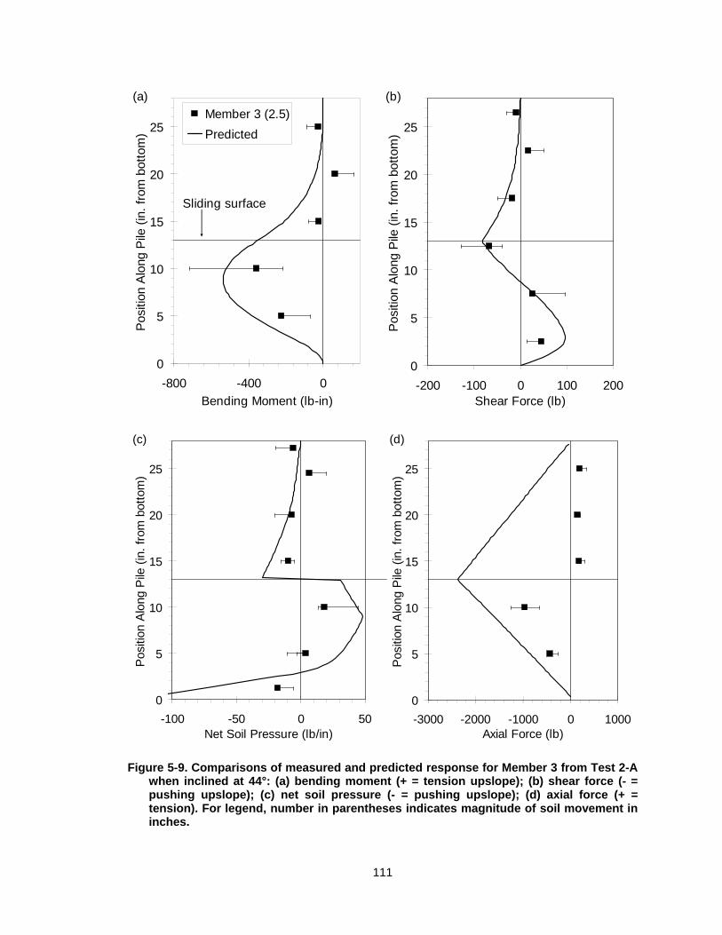
111

0

5

10

15

20

25

-800 -400 0


Pos

ition

Alo

ng P

ile (

in.

from

bot

tom

)

Member 3 (2.5)

Predicted

Sliding surface

(a)

0

5

10

15

20

25

-200 -100 0 100 200Shear Force (lb)

Pos

ition

Alo

ng P

ile (

in.

from

bot

tom

)

(b)

0

5

10

15

20

25

-100 -50 0 50Net Soil Pressure (lb/in)

Pos

ition

Alo

ng P

ile (

in.

from

bot

tom

)

(c)

0

5

10

15

20

25

-3000 -2000 -1000 0 1000Axial Force (lb)

Pos

ition

Alo

ng P

ile (

in.

from

bot

tom

)

(d)


112

5.2.2.2 Test 2-B

Twelve micropiles were installed without a capping beam in an A-frame arrangement

resulting in an S/D value of 9.6. All piles were battered 30 degrees upslope and downslope of the

line perpendicular to the slope face. The nominal diameters of all piles were 1.5 inches. The

model failed when inclined at 42 degrees. p-y analyses were conducted using LPile 5.0®,

attempting to match the predictions to measured values for Member 2 (inclined upslope) and

Member 3 (inclined downslope). Test parameters used for back-analyses of pile response for

Test 2-B are summarized in Table 5-11.




(in.) Sliding Depth

(in.)

34 0.2 3 6

40 0.3 18 11 42 1.4 16 11

Table 5-12. Back-calculated p-, y- and t-multipliers for Test 2-B.

Pile Batter Member



Downslope 3 0.2 1 1

Back-calculated p- and y-multipliers that produce the best fit between predicted and

measured moment profiles for both upslope and downslope members are summarized in Table

5-12. Results of p-y analysis with measured and predicted responses for Member 2 just prior to

failure are displayed in Figure 5-10. Good agreement among moment profiles is observed. Shear

force profiles display close agreement, and are similar to upslope member in Model 2-A. Soil

pressure predictions from p-y analysis match closely with calculated values. The near linear

increase in soil pressure with depth also indicates that the limit resistance was fully mobilized

from the pile head down to 10-in below the sliding surface. Result of t-z analysis for upslope pile

shows that decent match was obtained between the predicted and measured responses.

113

0

5

10

15

20

25

30

35

40

-2000 -1500 -1000 -500 0


Pos

ition

Alo

ng P

ile (

in.

from

bot

tom

)

Member 2 (1.4)

Predicted

(a)

Sliding surface

0

5

10

15

20

25

30

35

40

-200 -100 0 100 200

Shear Force (lb)P

ositi

on A

long

Pile

(in

. fr

om b

otto

m)

(b)

0

5

10

15

20

25

30

35

40


Pos

ition

Alo

ng P

ile (

in.

from

bot

tom

)

(c)

0

5

10

15

20

25

30

35

40

-2000 0 2000 4000Axial Force (lb)

Pos

ition

Alo

ng P

ile (

in.

from

bot

tom

)

(d)

Figure 5-10. Comparisons of measured and predicted response for Member 2 from Test 2-B when inclined at 42°: (a) bending moment (+ = tension upslope); (b) shear force (- = pushing upslope); (c) net soil pressure (- = pushing upslope); (d) axial force (+ = tension). For legend, number in parentheses indicates magnitude of soil movement in inches.

114

The p-multiplier of 0.2 and y-multiplier of 1.0 produced the closest match for data of

Member 3. Figure 5-11 shows predictions of p-y analysis along with measured and calculated

responses for the downslope member just prior to failure. Note that strain gage 7 malfunctioned

(at second level from pile head, facing downslope) and data for this strain gage was calculated by

taking the average of strains measured just above and below the malfunctioning gage. Figure

5-11a shows good agreement between measured and predicted moments. As a result of a good

agreement between moment profiles, calculated and predicted shear force and net soil pressure

profiles match closely as displayed in Figure 5-11d and Figure 5-11c, respectively. The quasi-

linear increase in net soil pressure from the pile head down to the sliding surface indicates that

the limit soil resistance was only mobilized above the sliding surface. The agreement between

measured and predicted axial force profiles for the downslope member (Figure 5-11d) is weak.

Measurements indicate that tensile load was mobilized above the sliding surface and

compressive load below the sliding surface. However, t-z analysis indicates that compression

load was mobilized along the full length of pile.

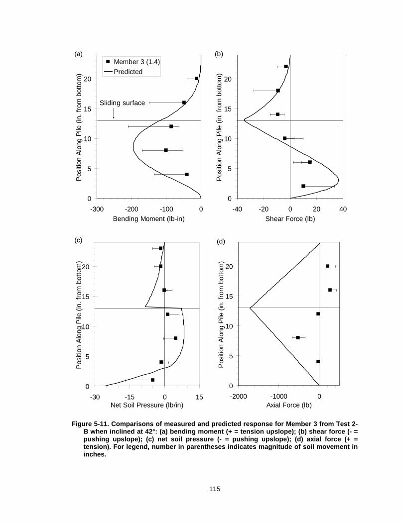
115

0

5

10

15

20

-300 -200 -100 0


Pos

ition

Alo

ng P

ile (

in.

from

bot

tom

)

Member 3 (1.4)

Predicted

(a)

Sliding surface

0

5

10

15

20

-40 -20 0 20 40

Shear Force (lb)P

ositi

on A

long

Pile

(in

. fr

om b

otto

m)

(b)

0

5

10

15

20


Pos

ition

Alo

ng P

ile (

in.

from

bot

tom

)

(c)

0

5

10

15

20

-2000 -1000 0Axial Force (lb)

Pos

ition

Alo

ng P

ile (

in.

from

bot

tom

)

(d)


116


Six tests were performed in Group 3. Three of these tests were reported by Boeckmann

(2006) and Textor (2007) as indicated in Table 5-13. For all tests in Group 3 piles were installed

with a capping beam in an A-frame arrangement with piles battered 30 degrees upslope and

downslope of the line perpendicular to the slope face as shown in Figure 4-1c. The pile response

analyses were performed using MU Pile Group to account for group effects. For analyses of test

results reported by Boeckmann (2006) and Textor (2007), predictions were matched with the

measured response for members reported as representative by Boeckmann (2006) and Textor

(2007). Horizontal bars in the figures indicate the range between values determined using upper

and lower bound interpretations of the data, while solid squares indicate values from rigorous

interpretations.

Table 5-13. Summary of Tests in Group 3. Test numbers with an asterisk indicate tests reported by Boeckman (2006) whereas test numbers with an apostrophe indicate tests reported by Textor (2007).



Batter Angle (deg.)


3A* 6 9.6 ±30 1.5

3B* 12 4.8 ±30 1.5

3C' 18 3.2 ±30 1.5

3D 10 5.8 ±30 1.5

3E 10 4.3 ±30 2.0

3F 6 7.2 ±30 2.0

5.2.3.1 Test 3-A

Six, 1.5-in diameter micropiles were installed through a capping beam in an A-frame

arrangement resulting in an S/D ratio of 9.6. The piles were battered 30 degrees upslope and

downslope of the line perpendicular to the slope face. The model failed at a slope inclination of 44

degrees. Pile response analyses were performed using MU Pile Group to account for group

effects between members. p- and y-multipliers were back-calculated attempting to match

predictions with measured responses for Member 2 (inclined upslope) and Member 3 (inclined

117

downslope). Test parameters used for back-analyses of pile response for Test 3-A and back-

calculated p- and y-multipliers are summarized in Table 5-14 and Table 5-15, respectively.




(in.) Sliding Depth

(in.)

30 0.1 13 10

38 0.3 18 11

42 0.8 28 15

44 1.0 27 14


Pile Batter Member


p-multiplier y-multiplier t-multiplier Upslope 2 0.18 0.83 40

Downlsope 3 1.35 1.0 40

The p-multiplier of 0.18 and y-multiplier of 0.8 were back-calculated to produce the best

fit with measured results for the upslope piles. Moment prediction and the response of Member 2

just prior to failure is shown in Figure 5-12a. The profiles match well in terms of shape, but the

magnitudes differ slightly with predicted values of moments being greater than measured values.

Moments predicted at the capping beam for both upslope and downslope members are ±890 lb-

in, indicating that moment equilibrium is satisfied at the pile cap. As a result of close agreement in

the shape of measured and predicted moments, shear force and net soil pressure profiles tend to

match closely. The predicted axial forces also show good agreement with measurements at most

points along the pile.

Figure 5-13 shows predictions of pile response along with the measured response for

Member 3 immediately before failure. The p-multiplier of 1.35 and y-multiplier of 1.0 were back-

calculated to have closest agreement between predicted and measured responses. Below the

sliding surface, both measured and predicted moments match closely in terms of shape and

magnitude. However, the agreement above the sliding surface is unknown, because there were

not any strain gages above the sliding surface. Similar to moment profiles, close agreements

118

between predicted and calculated shear force and net soil pressure profiles are observed (Figure

5-13b and Figure 5-13c). However, Figure 5-13d shows that a close match between the axial

force measurements and predictions is not observed, since measurements indicate mobilization

of tensile force at all measurement points while predictions show compressive force.

119

0

5

10

15

20

25

30

35

40

-1000 -500 0 500 1000


Pos

ition

Alo

ng P

ile (

in.

from

bot

tom

)

Predicted

Member 2(1.0)

Sliding surface

(a)

0

5

10

15

20

25

30

35

40

-200 -100 0 100 200Shear Force (lb)

Pos

ition

Alo

ng P

ile (

in.

from

bot

tom

)

(b)

0

5

10

15

20

25

30

35

40


Pos

ition

Alo

ng P

ile (

in.

from

bot

tom

)

(c)

0

5

10

15

20

25

30

35

40


Pos

ition

Alo

ng P

ile (

in.

from

bot

tom

)

(d)


120

0

5

10

15

20

25

30

35

-3000 -2000 -1000 0 1000Bending Moment (lb-in)

Pos

ition

Alo

ng P

ile (

in.

from

bot

tom

)

Predicted

Member 3(1.0)

Sliding surface

(a)

0

5

10

15

20

25

30

35


Pos

ition

Alo

ng P

ile (

in.

from

bot

tom

)

(b)

0

5

10

15

20

25

30

35

-250 -150 -50 50 150 250Net Soil Pressure (lb/in)

Pos

ition

Alo

ng P

ile (

in.

from

bot

tom

)

(c)

0

5

10

15

20

25

30

35

-2000 0 2000 4000 6000Axial Force (lb)

Pos

ition

Alo

ng P

ile (

in.

from

bot

tom

)

(d)


121

5.2.3.2 Test 3-B

Twelve, 1.5-in diameter micropiles were installed through a wooden capping beam for

Test 3-B, resulting in an S/D value of 4.8. Six of the members were installed 30 degrees upslope

and six were installed 30 degrees downslope of the line perpendicular to the slope face. The

model failed at a slope inclination of 47 degrees. The pile response analyses were performed

using MU Pile Group, attempting to match the predicted bending moments to the measured

response of Member 2 (inclined upslope) and Member 3 (inclined downslope). Test parameters

used for back-analyses of pile response for Test 3-B is summarized in Table 5-16. Back-

calculated multipliers are summarized in Table 5-17.




(in.) Sliding Depth

(in.)

30 0.03 30 23

40 0.05 28 25

44 0.2 32 26

46 0.6 32 24 47 1 32 24


Pile Batter Member



Downlsope 3 1.3 0.5 40

The p-multiplier of 0.3 and y-multiplier of 0.5 produced the best fit with measured results

for Member 2. The measured and predicted moments for the upslope member immediately

before failure are shown in Figure 5-14. The moment prediction matches well with measured data

below the failure surface, and follows the general trend of measurements above the failure

surface. Pile response analysis predicted a double curvature shaped moment distribution with a

maximum value above the sliding surface and little moment at the pile cap. This fact is a result of

sliding surface being relatively deep, in this case 32 inches. Figure 5-14b shows that predicted

122

shear force profile matches closely with calculated values at most points. A generally linear

increase in net soil pressure with depth (Figure 5-14c) indicates that the limit resistance was fully

mobilized along the most of the pile length. Figure 5-14d shows good agreement among

predicted and measured axial force profiles; both of them show that tensile load was mobilized

along the whole length of pile, with maximum measured values at similar depths. Predicted and

measured axial forces also match well for the upslope pile and indicate that little load was

transferred to the pile cap.

Figure 5-15 compares the predicted and measured response for Member 3 (inclined

downslope) just prior to failure. A back-calculated p-multiplier of 1.4 and y-multiplier of 0.5

produced the closest match with measured moments for Member 3. Both predicted and

measured profiles match reasonably well at four measurement points. Since the failure surface

for Member 3 was also relatively deep, in this case 24 inches, little moment was observed at the

pile cap. This is similar to moments predicted and measured for the upslope pile, indicating

moment equilibrium was satisfied. Calculated and predicted shear force profiles tend to match

well along the lower part of pile where moment agreement was strong. The maximum predicted

shear force for Member 3 is three times greater than the maximum predicted shear force for

Member 2, indicating that the downslope members provided three times more resistance. Similar

to the net soil pressure profile for Member 2, increasing value of soil pressure with depth

indicates that limit resistance was fully mobilized along most of the pile length for Member 3.

Measured and predicted axial force profiles show decent match as shown in Figure 5-15d.

123

0

5

10

15

20

25

30

35

40

-500 0 500 1000 1500Bending Moment (lb-in)

Pos

ition

Alo

ng P

ile (

in.

from

bot

tom

)

Predicted

Member 2(1.0)

Sliding surface

(a)

0

5

10

15

20

25

30

35

40

-300 -200 -100 0 100 200Shear Force (lb)

Pos

ition

Alo

ng P

ile (

in.

from

bot

tom

)

(b)

0

5

10

15

20

25

30

35

40


Pos

ition

Alo

ng P

ile (

in.

from

bot

tom

)

(c)

0

5

10

15

20

25

30

35

40

0 2000 4000 6000Axial Force (lb)

Pos

ition

Alo

ng P

ile (

in.

from

bot

tom

)

(d)


124

0

5

10

15

20

25

30

-2000 0 2000Bending Moment (lb-in)

Pos

ition

Alo

ng P

ile (

in.

from

bot

tom

)

Predicted

Member 3(1.0)

Slidingsurface

(a)

0

5

10

15

20

25

30

-800 -400 0 400Shear Force (lb)

Pos

ition

Alo

ng P

ile (

in.

from

bot

tom

)

(b)

0

5

10

15

20

25

30

-300 -200 -100 0 100 200 300Net Soil Pressure (lb/in)

Pos

ition

Alo

ng P

ile (

in.

from

bot

tom

)

(c)

0

5

10

15

20

25

30

-8000 -4000 0 4000Axial Force (lb)

Pos

ition

Alo

ng P

ile (

in.

from

bot

tom

)

(d)


125

5.2.3.3 Test 3-C

Eighteen, 1.5-in diameter reinforcing members were installed through a capping beam for

Test 3-C in an A-frame arrangement, resulting in an S/D ratio of 3.2. Piles were battered 30

degrees upslope and downslope of the line perpendicular to the slope face. The model failed

when inclined at 43 degrees. MU Pile Group was used for pile response analyses and predictions

were attempted to match with responses for Members 2 and 3, which are downslope and upslope

piles, respectively. Test parameters used for back-analyses of pile response for Test 3-C are

summarized in Table 5-18.




(in.) Sliding Depth

(in.)

30 0.2 26 12

38 0.4 26 12

40 0.45 26 14

42 0.5 26 11

43 0.7 26 14

Table 5-19. Back-calculated p-, y- and t-multipliers for Test 3-C.

Pile Batter Member




Comparisons between predictions and response for Member 3 immediately before failure

can be seen in Figure 5-16. At this stage, Strain gage 3 (at third level from pile head, facing

upslope) had shorted out and the fourth pair of gages showed 11960 lb-in moment. This value is

almost double the moment capacity of pile, which is 6400 lb-in. Nevertheless, a p-multiplier of 0.4

and y-multiplier of 0.33 resulted in a close match among the prediction and measured bending

moment. The predicted and calculated shear force profiles show good agreement, with the

resulting maximum values located at similar depth. Figure 5-16c shows that agreement between

the predicted and calculated net soil pressures is decent. Increase in net soil pressure values with

126

depth indicates that limit resistance was mobilized along the most of the pile length. Test

measurements show tensile forces between 24000 lb and 45000 lb in the middle of the pile.

These values are greater than the axial capacity of pile, which is 22000 lb. Therefore both axial

force profiles lacked agreement as shown in Figure 5-16d.

The closest agreement among bending moment profiles for Member 2 was obtained

using a p-multiplier of 1.8 and y-multiplier of 0.33. Figure 5-17 compares the predicted and

measured response for Member 2 when the model was inclined at 42 degrees, because strain

gage 1 (at first level from pile head, facing upslope) shorted out at a slope inclination of 43

degrees. Figure 5-17a shows that both predicted and measured profiles are consistent with one

another. Predicted moment 3-in below the capping beam is close the moment from the rigorous

interpretation. The predicted and calculated shear force profiles show generally good agreement

at most points. However, net soil pressure and axial force profiles lacked agreement unlike

moment and shear force profiles.

127

0

5

10

15

20

25

30

35

-2000 -1000 0 1000 2000Bending Moment (lb-in)

Pos

ition

Alo

ng P

ile (

in.

from

bot

tom

)

Member 3(0.7)

Predicted

Sliding surface

(a)

0

5

10

15

20

25

30

35

-1000 -500 0 500 1000Shear Force (lb)

Pos

ition

Alo

ng P

ile (

in.

from

bot

tom

)

(b)

0

5

10

15

20

25

30

35


Pos

ition

Alo

ng P

ile (

in.

from

bot

tom

)

(c)

0

5

10

15

20

25

30

35

-10000 -5000 0 5000 10000Axial Force (lb)

Pos

ition

Alo

ng P

ile (

in.

from

bot

tom

)

(d)

Figure 5-16. Comparisons of measured and predicted response for Member 3 from Test 3-C when inclined at 43°: (a) bending moment (+ = tension upslope); (b) shear force (- = pushing upslope); (c) net soil pressure (- = pushing upslope); (d) axial force (+ = tension). For legend, number in parentheses indicates magnitude of soil movement in inches.

128

0

5

10

15

20

25

30


Pos

ition

Alo

ng P

ile (

in.

from

bot

tom

)

Predicted

Member 2(0.5)

Sliding surface

(a)

0

5

10

15

20

25

30

-400 -200 0 200Shear Force (lb)

Pos

ition

Alo

ng P

ile (

in.

from

bot

tom

)

(b)

0

5

10

15

20

25

30


Pos

ition

Alo

ng P

ile (

in.

from

bot

tom

)

(c)

0

5

10

15

20

25

30


Pos

ition

Alo

ng P

ile (

in.

from

bot

tom

)

(d)

Figure 5-17. Comparisons of measured and predicted response for Member 2 from Test 3-C when inclined at 42°: (a) bending moment (+ = tension upslope); (b) shear force (- = pushing upslope); (c) net soil pressure (- = pushing upslope); (d) axial force (+ = tension). For legend, number in parentheses indicates magnitude of soil movement in inches.

129

5.2.3.4 Test 3-D

Ten, 1.5-in diameter reinforcing members were installed through a capping beam to

create an A-frame arrangement for Test 3-D. Upslope and downslope piles were divided equally

and inclined 30 degrees upslope and 30 degrees downslope of the line perpendicular to the slope

face. Resulting S/D ratio was of 5.8 and model failed at slope inclination of 47 degrees. Members

1 and 3 were battered upslope while Members 2 and 4 were battered downslope. Three of the

instrumented members were monitored continuously while Member 4 was monitored manually

and served as back up for Member 2, in case it had unreasonable results. Member 1 had two

strain gages short out when model inclined at 47 degrees, and Member 2 had only one strain

gage short out at slope inclination of 36 degrees. On the other hand, strain gages on Members 3

and 4 did not experience problem. Pile response analyses were performed using MU Pile Group,

attempting to match predictions to response for Members 2 and 3. Test parameters used for

back-analyses of pile response for Test 3-D and back-calculated p- and y-multipliers are

summarized in Table 5-20 and Table 5-21, respectively.

Table 5-20. Test parameters used for back-analyses of pile response for Test 3-D.



(in.) Sliding Depth

(in.)

30 0.6 16 12 40 0.8 14 16 43 1 14 16 45 1.4 16 15 46 1.8 16 16

Table 5-21. Back-calculated p-, y- and t-multipliers for Test 3-D.

Pile Batter Member No Back-calculated Multipliers p-multiplier y-multiplier t-multiplier

Upslope 1, 3 0.35 0.5 40 Downlsope 2, 4 1.4 0.5 40

Closest agreement between predictions and response for Member 3 is obtained using p-

multiplier of 0.35 and y-multiplier of 0.5. Comparisons between prediction of analyses and

measured response for upslope members just prior to failure are shown in Figure 5-18. Close

130

agreement between predicted and measured moment profiles for upslope piles can be seen in

Figure 5-18a. Result of pile response analysis indicates 530 lb-in moment at the pile cap as a

result of load transfer among the pile group. As shown in Figure 5-18b and Figure 5-18c,

predicted shear force and net soil pressure profiles also display good agreement with calculated

response. However, decent match between predicted and measured axial force responses for

Members 2 and 4 is observed as displayed in Figure 5-18d.

The p-multiplier of 1.4 and y-multiplier of 0.5 were back-calculated to produce best fit with

response for Member 2. Figure 5-19 compares the predicted and measured response for

downslope members just prior to failure. Predicted bending moment (Figure 5-19a) from pile

response analyses matches the measurements at most of the points except one, where they

indicated same magnitude but different in sign. Close agreement between predicted and

calculated shear force profiles is observed, except the first point from pile head. Both shear force

profiles indicate maximum values at the same depth. Maximum shear force for downslope

member is predicted as four times greater than the amount predicted for upslope member,

indicating downslope member provided four times more resistance. Predicted net soil pressure

matches closely with calculated response, as a result of good agreement between shear force

profiles. As shown in Figure 5-19c, increasing in net soil pressure value down to 4-in below the

sliding surface indicates the mobilization of limit resistance. A good agreement between axial

force profiles is not observed, since predictions show compressive force along the full length of

pile while most of the measurements indicated tensile force.

131

0

5

10

15

20

25

30

35


Pos

ition

Alo

ng P

ile (

in.

from

bot

tom

)

Member 3(1.8)Predicted

Member 1

Sliding surface

(a)

0

5

10

15

20

25

30

35


Pos

ition

Alo

ng P

ile (

in.

from

bot

tom

)

(b)

0

5

10

15

20

25

30

35

-30 0 30 60Net Soil Pressure (lb/in)

Pos

ition

Alo

ng P

ile (

in.

from

bot

tom

)

(c)

0

5

10

15

20

25

30

35

-2000 0 2000 4000 6000Axial Force (lb)

Pos

ition

Alo

ng P

ile (

in.

from

bot

tom

)

(d)

Figure 5-18. Comparisons of measured and predicted response for upslope members from Test 3-D when inclined at 46°: (a) bending moment (+ = tension upslope); (b) shear force (- = pushing upslope); (c) net soil pressure (- = pushing upslope); (d) axial force (+ = tension). For legend, number in parentheses indicates magnitude of soil movement in inches. Horizontal bars indicate upper and lower bound for Member 3.

132

0

5

10

15

20

25

-1500 -1000 -500 0 500 1000Bending Moment (lb-in)

Pos

ition

Alo

ng P

ile (

in.

from

bot

tom

)


Member 4

Slidingsurface

(a)

0

5

10

15

20

25

-300 -150 0 150Shear Force (lb)

Pos

ition

Alo

ng P

ile (

in.

from

bot

tom

)

(b)

0

5

10

15

20

25


Pos

ition

Alo

ng P

ile (

in.

from

bot

tom

)

(c)

0

5

10

15

20

25

-3000 0 3000 6000 9000Axial Force (lb)

Pos

ition

Alo

ng P

ile (

in.

from

bot

tom

)

(d)

Figure 5-19. Comparisons of measured and predicted response for downslope members from Test 3-D when inclined at 46°: (a) bending moment (+ = tension upslope); (b) shear force (- = pushing upslope); (c) net soil pressure (- = pushing upslope); (d) axial force (+ = tension). For legend, number in parentheses indicates magnitude of soil movement in inches. Horizontal bars indicate upper and lower bound for Member 2.

133

5.2.3.5 Test 3-E

Six, 2.0-in diameter reinforcing members were installed for Test 3-E in an A-frame

arrangement resulting in an S/D ratio of 4.3. Piles were battered 30 degrees upslope and

downslope of the line perpendicular to the slope face. A wooden capping beam was used to

attach members to each other. The model failed at slope inclination of 47 degrees. Members 1

and 3 were battered upslope while Members 2 and 4 were battered downslope. Three of the

members were monitored continuously while data for Member 4 was collected manually and

served as back up for Member 2, in case it had unreasonable results. One of the strain gages on

Member 1 shorted out while strain gages on Members 2, 3 and 4 did not experience any problem.

Therefore, pile response analyses were conducted using MU Pile Group, attempting to match

predictions to response for Member 2 and Member 3. Test parameters used for back-analyses of

pile response for Test 3-E is presented in Table 5-22.

Table 5-22. Test Parameters used for back-analyses of pile response for Test 3-E.



(in.) Sliding Depth

(in.) 36 0.1 14 12 40 0.25 8 10 43 0.5 13 13 44 0.9 16 16 45 1.45 14 16

Table 5-23. Back-calculated p-, y- and t-multipliers for Test 3-E.



Back-calculated p- and y-multipliers that produce the best fit with measured results for

upslope and downslope members are summarized in Table 5-23. Figure 5-20 compares the

measured and predicted response for upslope members at slope inclination of 45 degrees.

Although the predicted moment profile does not match with measured response as well as in Test

3-D, good agreement is observed among predicted and measured moment profiles at

134

intermediate tilt stages. As an example, predicted and measured response for Member 3 at slope

inclination of 43 degrees is shown in Figure 5-21. It is displayed in Figure 5-21a that good

agreement among predicted and measured moments is apparent below sliding surface as well as

3-in below the capping beam. The predicted shear force profile shows close match with

calculated values (when model inclined at 43 degrees) along most of the pile length as shown in

Figure 5-21b. However, shear force agreement is not as good at slope inclination of 45 degrees.

As a cumulative result of weak agreements among moment and shear profiles at 45 degrees of

slope angle, net soil pressures profiles do not display good agreement. However, better match for

soil pressure profiles is obtained at slope inclination of 43 degrees. The axial force predictions at

both slope inclinations do not display good agreement with measured response.

Comparisons between predicted and measured response for downslope members just

prior to failure are displayed in Figure 5-22. Considering the data from Member 2, shape of

predicted bending moment is similar to shape of measured moment profile. Generally, predictions

under estimated the moment, and indicated maximum moment at pile cap which is -930 lb-in.

Same amount of moment but different in sign is observed on upslope pile, indicating that moment

equilibrium at pile cap was established. As a result of moment profiles being similar in terms of

shape, shear force prediction, in fact showed better agreement with calculated shear force

values. Maximum mobilized shear force at the sliding surface is -320 lb, which is about three

times greater than the maximum shear force on upslope pile, indicating that downslope pile

provided three times more resistance. As displayed in Figure 5-22c, there is a close match

between predicted and calculated soil pressures, especially at first three point from pile head. An

increase in prediction of net soil pressure until failure surface indicates that limit soil resistance

was fully mobilized only above the failure surface. Result of pile response analysis and measured

response for downslope members lacked agreement similar to axial force profiles for upslope

members.

135

0

5

10

15

20

25

30

35


Pos

ition

Alo

ng P

ile (

in.

from

bot

tom

)

Member 3(1.45)

Predicted

Member 1

(a)

Sliding surface

0

5

10

15

20

25

30

35

-150 -100 -50 0 50 100 150Shear Force (lb)

Pos

ition

Alo

ng P

ile (

in.

from

bot

tom

)

(b)

0

5

10

15

20

25

30

35


Pos

ition

Alo

ng P

ile (

in.

from

bot

tom

)

(c)

0

5

10

15

20

25

30

35

-2000 0 2000 4000Axial Force (lb)

Pos

ition

Alo

ng P

ile (

in.

from

bot

tom

)

(d)

Figure 5-20. Comparisons of measured and predicted response for upslope members from Test 3-E when inclined at 45°: (a) bending moment (+ = tension upslope); (b) shear force (- = pushing upslope); (c) net soil pressure (- = pushing upslope); (d) axial force (+ = tension). For legend, number in parentheses indicates magnitude of soil movement in inches. Horizontal bars indicate upper and lower bound for Member 3.

136

0

5

10

15

20

25

30

35


Pos

ition

Alo

ng P

ile (

in.

from

bot

tom

)

Member 3(0.5)

Predicted

Member 1

Slidingsurface

(a)

0

5

10

15

20

25

30

35


Pos

ition

Alo

ng P

ile (

in.

from

bot

tom

)

2

(b)

0

5

10

15

20

25

30

35


Pos

ition

Alo

ng P

ile (

in.

from

bot

tom

)

(c)

0

5

10

15

20

25

30

35

-2000 -1000 0 1000 2000 3000Axial Force (lb)

Pos

ition

Alo

ng P

ile (

in.

from

bot

tom

)

(d)

Figure 5-21. Comparisons of measured and predicted response for upslope members from Test 3-E when inclined at 43°: (a) bending moment (+ = tension upslope); (b) shear force (- = pushing upslope); (c) net soil pressure (- = pushing upslope); (d) axial force (+ = tension). For legend, number in parentheses indicates magnitude of soil movement in inches. Horizontal bars indicate upper and lower bound for Member 3.

137

0

5

10

15

20

25


Pos

ition

Alo

ng P

ile (

in.

from

bot

tom

)


Member 4

(a)

Sliding surface

0

5

10

15

20

25


Pos

ition

Alo

ng P

ile (

in.

from

bot

tom

)

(b)

0

5

10

15

20

25


Pos

ition

Alo

ng P

ile (

in.

from

bot

tom

)

(c)

0

5

10

15

20

25

-4000 -2000 0 2000 4000 6000Axial Force (lb)

Pos

ition

Alo

ng P

ile (

in.

from

bot

tom

)

(d)

Figure 5-22. Comparisons of measured and predicted response for downslope members from Test 3-E when inclined at 45°: (a) bending moment (+ = tension upslope); (b) shear force (- = pushing upslope); (c) net soil pressure (- = pushing upslope); (d) axial force (+ = tension). For legend, number in parentheses indicates magnitude of soil movement in inches. Horizontal bars indicate upper and lower bound for Member 2.

138

5.2.3.6 Test 3-F

Six, 2.0-in diameter micropiles were installed through capping beam for Test 3-F in an A-

frame arrangement. Piles were battered 30 degrees upslope and downslope of the line

perpendicular to the slope face, resulting in an S/D ratio of 7.2. The model failed at a slope

inclination of 46 degrees. Members 2 and 3 were battered upslope while Members 1 and 4 were

battered downslope. Members 1, 2 and 3 were monitored continuously while data for Member 4

was collected manually prior to each tilt increment and served as back up for Member 1, in case

strain gages short out. Two of the strain gages on Member 2 shorted out during the test while

none of the strain gages for Member 3 had problem. Member 1 had one strain gage and Member

4 had two strain gages shorted out. Therefore, pile response analyses were performed using MU

Pile group to match predictions with response for Members 1 and 3. Test parameters used for

back-analyses of pile response for Test 3-F are described in Table 5-23.

Table 5-24. Test parameters used for back-analyses of pile response for Test 3-F.



(in.) Sliding Depth

(in.) 34 0.25 14 15 36 0.3 13 16 40 0.8 13 16 45 1.3 13 16

Table 5-25. Back-calculated p-, y- and t-multipliers for Test 3-F.

Pile Batter Member


p-multiplier y-multiplier t-multiplier Upslope 2, 3 0.25 0.65 40

Downlsope 1, 4 1.5 0.8 40

Multipliers that produced the best fit among predictions and response for Members 1 and

3 are summarized in Table 5-25. Figure 5-23 compares the predicted and measured response for

upslope piles just prior to failure. Moment prediction matches fairly well with test measurements

above the sliding surface and falls between the ranges of measured data below the sliding

surface. Maximum moment is predicted at pile cap as 825 lb-in, and this is a result of sliding

139

depth being relatively shallow, which is causing load to be concentrated at pile cap. The match

between predicted and calculated shear force profiles is shown in Figure 5-23b. Although

calculated response for Member 2 matches closely with predictions, better agreement for

Member 3 is not observed. Similarly, agreement for net soil pressure profiles is also decent as

shown in Figure 5-23c. An increase in prediction of net soil pressure down to sliding surface

indicates the mobilization of limit resistance. As shown in Figure 5-23d, predicted and measured

axial force profiles only matches 3-in below the capping beam and lack agreement at the

remaining points.

The p-multiplier of 1.5 and y-multiplier of 0.8 were found as the multipliers that produced

the best fit with measured results for Member 1. Measured moment responses for downslope

members are shown in Figure 5-24a, which is similar to response of Member 2 in Test 3-E

(Figure 5-22a). General agreement among predicted and measured moment profiles seems

good. As shown in Figure 5-24b, good match between predicted and calculated shear force

profiles is observed below and right above the sliding surface. However, close match is not

observed for net soil pressure profiles as displayed in Figure 5-24c. Axial force measurements

generally show tensile force along the pile and no clear trend exists among these measurements.

Predictions show compressive force along the pile similar for any dowslope member. Figure

5-24d shows the distinction between measured and predicted axial forces.

140

0

5

10

15

20

25

30

35


Pos

ition

Alo

ng P

ile (

in.

from

bot

tom

)

Member 3(1.25)

Predicted

Member 2

Sliding surface

(a)

0

5

10

15

20

25

30

35

-120 -90 -60 -30 0 30Shear Force (lb)

Pos

ition

Alo

ng P

ile (

in.

from

bot

tom

)

(b)

0

5

10

15

20

25

30

35


Pos

ition

Alo

ng P

ile (

in.

from

bot

tom

)

(c)

0

5

10

15

20

25

30

35

-1000 0 1000 2000 3000Axial Force (lb)

Pos

ition

Alo

ng P

ile (

in.

from

bot

tom

)

(d)

Figure 5-23. Comparisons of measured and predicted response for upslope members from Test 3-F when inclined at 45°: (a) bending moment (+ = tension upslope); (b) shear force (- = pushing upslope); (c) net soil pressure (- = pushing upslope); (d) axial force (+ = tension). For legend, number in parentheses indicates magnitude of soil movement in inches. Horizontal bars indicate upper and lower bound for Member 3.

141

0

5

10

15

20

25


Pos

ition

Alo

ng P

ile (

in.

from

bot

tom

)

Member 1(1.25)

Predicted

Member 4

Sliding surface

(a)

0

5

10

15

20

25


Pos

ition

Alo

ng P

ile (

in.

from

bot

tom

)

(b)

0

5

10

15

20

25


Pos

ition

Alo

ng P

ile (

in.

from

bot

tom

)

(c)

0

5

10

15

20

25

-5000 0 5000 10000Axial Force (lb)

Pos

ition

Alo

ng P

ile (

in.

from

bot

tom

)

(d)

Figure 5-24. Comparisons of measured and predicted response for downslope members from Test 3-F when inclined at 45°: (a) bending moment (+ = tension upslope); (b) shear force (- = pushing upslope); (c) net soil pressure (- = pushing upslope); (d) axial force (+ = tension). For legend, number in parentheses indicates magnitude of soil movement in inches. Horizontal bars indicate upper and lower bound for Member 1.

142


Three tests were performed in Group 3. Two of these tests were reported by Textor

(2007) as indicated in Table 5-26. Piles were installed through capping beam in an A-frame

arrangement with piles battered 15 degrees upslope and downslope of the line perpendicular to

the slope face as shown in Figure 4-1d. The pile response analyses were performed using MU

Pile Group to account for group effects. For analyses of test results reported by Textor (2007), p-

and y-multipliers were back-calculated, attempting to match the predictions to response for

members reported as representative by Textor (2007). Horizontal bars in the figures indicate the

range between values determined using upper and lower bound interpretations of the data, while

solid squares indicate values from the rigorous interpretations.

Table 5-26. Summary of Tests in Group 4. Test numbers with an apostrophe indicate tests reported by Textor (2007).

Test No

Number of Piles


Batter Angle (deg.)

Nominal Pile

Diameter (in)

4A’ 6 9.6 ±15 1.5

4B’ 12 4.8 ±15 1.5

4C 18 3.2 ±15 2.0

5.2.4.1 Test 4-A

Six, 1.5-in micropiles were installed through a wooden capping beam to create an A-

frame arrangement resulting in an S/D ratio of 9.6. All piles were battered 15 degrees upslope

and downslope of the line perpendicular to the slope face. The model failed at a slope inclination

of 40 degrees. MU Pile Group was performed to back-calculated p- and y-multipliers that produce

the best fit with response for Members 1 and 2, which were inclined as the upslope and

downslope piles, respectively. Test parameters used for back-analyses of pile response for Test

4-A is summarized in Table 5-27.

143




(in.) Sliding Depth

(in.) 30 0.2 10 12 36 0.3 12 16 38 0.5 12 16



Upslope 1 0.3 0.9 40 Downlsope 2 1.2 1 40

The p-multiplier of 0.3 and y-multiplier of 0.9 were back-calculated as best fit multipliers

as shown in Table 5-28. Predicted moment profile shows close match with response for Member

1, as displayed in Figure 5-25a. The measured moment profile belongs to stage just prior to

failure. A good agreement exists among predicted and calculated shear force responses as a

result of close match between moment profiles as shown in Figure 5-25b. However, agreement

among net soil pressure profiles is not as close as agreements in moment and shear force

profiles. Nevertheless, predicted response matches some what close with test data below the

sliding surface. An increase in net soil pressure value from pile head down to 4-in below the

sliding surface indicates the mobilization of limit resistance. The axial force prediction show

tensile force along the full length of pile, and it matches decent with test measurements, except at

the middle of pile as displayed in Figure 5-25d.

Predicted moment profile was matched with measurements for Member 2, using p-

multiplier of 1.2 and y-multiplier 1.0. Similar to presented data for Member 1, comparisons

between predicted and measured responses were made for stage just prior to failure. A close

match below the sliding surface and near the capping beam is observed as shown in Figure

5-26a. Predicted moment at pile cap is -470 lb-in, which is identical to prediction on upslope pile,

but different in sign, indicating that model satisfied moment equilibrium at pile cap. Figure 5-26b

compares the predicted and calculated shear force responses. Both profiles show difference near

the sliding surface and 6-in below the pile cap, but display close match at the remaining points. A

144

good agreement for net soil pressure profiles is not observed, as shown in Figure 5-26c. Unlike

the axial force measurements for most downslope members, values of prediction falls between

the ranges of upper and lower bound near the sliding surface as well as below the capping beam,

and prediction generally display close match with measurements.

145

0

5

10

15

20

25

30


Pos

ition

Alo

ng P

ile (

in.

from

bot

tom

)

Member 1(0.5)

Predicted

Sliding surface

(a)

0

5

10

15

20

25

30


Pos

ition

Alo

ng P

ile (

in.

from

bot

tom

)

(b)

0

5

10

15

20

25

30


Pos

ition

Alo

ng P

ile (

in.

from

bot

tom

)

(c)

0

5

10

15

20

25

30

-1000 0 1000 2000 3000Axial Force (lb)

Pos

ition

Alo

ng P

ile (

in.

from

bot

tom

)

(d)


146

0

5

10

15

20

25


Pos

ition

Alo

ng P

ile (

in.

from

bot

tom

)

Predicted

Member 2(0.5)

Sliding surface

(a)

0

5

10

15

20

25

-400 -200 0 200Shear Force (lb)

Pos

ition

Alo

ng P

ile (

in.

from

bot

tom

)

(b)

0

5

10

15

20

25

-100 -50 0 50 100 150Net Soil Pressure (lb/in)

Pos

ition

Alo

ng P

ile (

in.

from

bot

tom

)

(c)

0

5

10

15

20

25

-4000 -2000 0 2000 4000Axial Force (lb)

Pos

ition

Alo

ng P

ile (

in.

from

bot

tom

)

(d)


147

5.2.4.2 Test 4-B

Twelve, 1-5-in micropiles were installed through a wooden capping beam for Test 4-B in

an A-frame arrangement with 15 degrees upslope and downslope of the line perpendicular to the

slope face, resulting in an S/D value of 4.8. The model failed when it was inclined at 44 degrees.

Pile response analyses were conducted using MU Pile Group to match predictions to measured

moments for Members 2 and 3. It is reported by Textor (2007) that data acquisition system did

not record any data until 40 degrees of slope angle. Therefore, all the moment measurements

were interpreted based on strains zeroed at beginning of 40 degrees slope angle. Test

parameters used for back-analyses of pile response for Test 4-A is summarized in Table 5-29.




(in.) Sliding Depth

(in.)

41 0.1 14 12 42 0.25 12 12 43 0.7 18 12


Pile Batter Member




Multipliers that produce the best fit with measured response for Members 2 and 3 are

summarized in Table 5-30. The pile response analysis produced a moment profile that matches

fairly well with measured response in terms of general shape. Furthermore, values of predictions

are identical to moments from rigorous interpretations at 3-in below the capping beam and near

the pile tip. Comparisons displayed in Figure 5-27 are from the data obtained just prior to failure.

Better match between predicted and measured responses were established for earlier stages of

the test. Therefore, a comparison at earlier stage is presented as an example in Figure 5-28. The

shear force prediction (just prior to failure) shows decent match with calculated response as

opposed to close match at earlier stage as shown in Figure 5-28b. Similarly, the predicted and

148

calculated net soil pressure profiles show better match at earlier stage as well. In Figure 5-28c,

quasi-linear increase in net soil pressure values from pile head down to sliding surface indicates

that limit resistance was only mobilized along the pile length above the failure surface. However,

an increase in Figure 5-27c shows that limit resistance was fully mobilized from pile head down to

4-in below sliding surface just prior to failure. The predicted and measured axial force profiles

generally show good agreement, especially at earlier stage. The predicted response shows

tensile force along the whole length of pile, which falls between the upper and lower bound

interpretations at most points. Agreement is strong below the failure surface and near the capping

beam just prior to failure. At slope inclination of 42 degrees, axial force profiles show good

agreement at most points, except right below the sliding surface.

The p- and y-multipliers were back-calculated as 1.3 and 0.8, respectively, which

produced the best fit with response for Member 2. Figure 5-29a compares the predicted and

measured responses just prior to failure. There is a good agreement below the sliding surface,

and distinction above. However, values are almost identical, but different in sign. The agreement

among shear force profiles is strong below the sliding surface as a result of close match in

moment profiles. Predictions for both upslope and downslope members show the same amount

of shear force at the sliding surface just prior to failure, which is about -150 lb, indicating both

members provided same amount of resistance (considering only lateral performance). Decent

match is observed for net soil pressure profiles. Increase in net soil pressure value down to

sliding depth indicates that limit resistance was mobilized only above the failure surface and not

below, similar to upslope member. The predicted axial force profiles show mobilization of

compression force along the pile length. However, close match is only obtained at fourth and fifth

level from pile head.

.

149

0

5

10

15

20

25

30


Pos

ition

Alo

ng P

ile (

in.

from

bot

tom

)

Member 3(0.7)

Predicted

Slidingsurface

(a)

0

5

10

15

20

25

30

-400 -200 0 200 400Shear Force (lb)

Pos

ition

Alo

ng P

ile (

in.

from

bot

tom

)

(b)

0

5

10

15

20

25

30


Pos

ition

Alo

ng P

ile (

in.

from

bot

tom

)

(c)

0

5

10

15

20

25

30

-2000 0 2000 4000 6000 8000Axial Force (lb)

Pos

ition

Alo

ng P

ile (

in.

from

bot

tom

)

(d)


150

0

5

10

15

20

25

30


Pos

ition

Alo

ng P

ile (

in.

from

bot

tom

)

Member 3(0.25)

Predicted

Slidingsurface

(a)

0

5

10

15

20

25

30


Pos

ition

Alo

ng P

ile (

in.

from

bot

tom

)

(b)

0

5

10

15

20

25

30


Pos

ition

Alo

ng P

ile (

in.

from

bot

tom

)

(c)

0

5

10

15

20

25

30

0 500 1000 1500 2000Axial Force (lb)

Pos

ition

Alo

ng P

ile (

in.

from

bot

tom

)

(d)


151

0

5

10

15

20

25


Pos

ition

Alo

ng P

ile (

in.

from

bot

tom

)

Member 2(0.7)

Predicted

Sliding surface

(a)

0

5

10

15

20

25

-150 -75 0 75 150Shear Force (lb)

Pos

ition

Alo

ng P

ile (

in.

from

bot

tom

)

(b)

0

5

10

15

20

25


Pos

ition

Alo

ng P

ile (

in.

from

bot

tom

)

(c)

0

5

10

15

20

25

-2500 -1500 -500 500 1500Axial Force (lb)

Pos

ition

Alo

ng P

ile (

in.

from

bot

tom

)

(d)


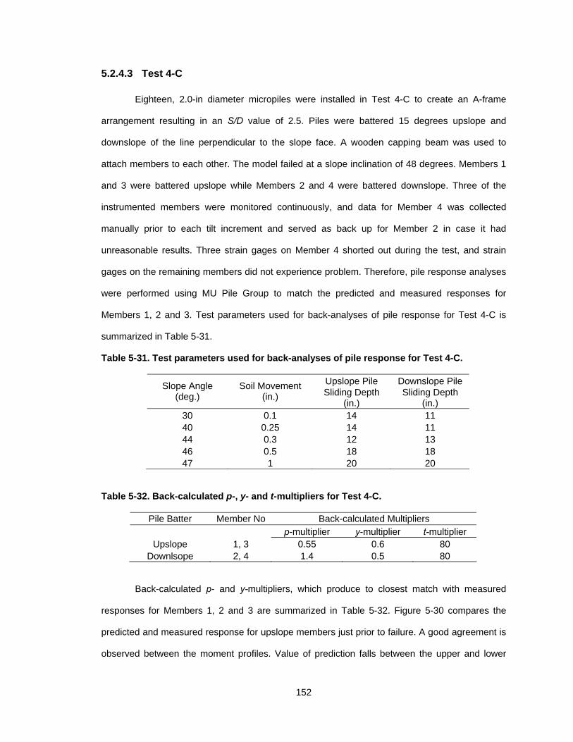
152

5.2.4.3 Test 4-C

Eighteen, 2.0-in diameter micropiles were installed in Test 4-C to create an A-frame

arrangement resulting in an S/D value of 2.5. Piles were battered 15 degrees upslope and

downslope of the line perpendicular to the slope face. A wooden capping beam was used to

attach members to each other. The model failed at a slope inclination of 48 degrees. Members 1

and 3 were battered upslope while Members 2 and 4 were battered downslope. Three of the

instrumented members were monitored continuously, and data for Member 4 was collected

manually prior to each tilt increment and served as back up for Member 2 in case it had

unreasonable results. Three strain gages on Member 4 shorted out during the test, and strain

gages on the remaining members did not experience problem. Therefore, pile response analyses

were performed using MU Pile Group to match the predicted and measured responses for

Members 1, 2 and 3. Test parameters used for back-analyses of pile response for Test 4-C is

summarized in Table 5-31.




(in.) Sliding Depth

(in.) 30 0.1 14 11 40 0.25 14 11 44 0.3 12 13 46 0.5 18 18 47 1 20 20

Table 5-32. Back-calculated p-, y- and t-multipliers for Test 4-C.



Back-calculated p- and y-multipliers, which produce to closest match with measured

responses for Members 1, 2 and 3 are summarized in Table 5-32. Figure 5-30 compares the

predicted and measured response for upslope members just prior to failure. A good agreement is

observed between the moment profiles. Value of prediction falls between the upper and lower

153

bound interpretations for Member 1 below the sliding surface as well as near the capping beam.

Moment profiles also indicate the maximum moments below the sliding surface. The predicted

and calculated shear force profiles show close match with one another as shown in Figure 5-30b.

However, decent agreement is observed for net soil pressure profiles as displayed in Figure

5-30c. The axial force prediction matches fairly well with measurements. Both predicted and

measured response for upslope members show the maximum axial force values about at the

same depth.

Figure 5-31 compares the predicted and measured response for downslope members

just prior to failure. Unlike the good agreement observed in moment profiles for upslope

members, close match was not obtained for downslope members as shown in Figure 5-31.

However, general trends of measured and predicted moments show similarity above the sliding

surface. Therefore, shear force and net soil pressure responses match closely at upper part of

pile as displayed in Figure 5-31b and Figure 5-31c, respectively. The axial force data from

interpretations suggest the mobilization of tensile force at all measurement points. However,

predictions indicate compressive force along the full length of pile. Therefore, a good agreement

was not established among axial force responses for downslope members.

154

0

5

10

15

20

25

30

35


Pos

ition

Alo

ng P

ile (

in.

from

bot

tom

)


Member 3

Sliding surface

(a)

0

5

10

15

20

25

30

35

-400 -200 0 200Shear Force (lb)

Pos

ition

Alo

ng P

ile (

in.

from

bot

tom

)

(b)

0

5

10

15

20

25

30

35


Pos

ition

Alo

ng P

ile (

in.

from

bot

tom

)

(c)

0

5

10

15

20

25

30

35

0 5000 10000 15000Axial Force (lb)

Pos

ition

Alo

ng P

ile (

in.

from

bot

tom

)

(d)

Figure 5-30. Comparisons of measured and predicted response for upslope members from Test 4-C when inclined at 47°: (a) bending moment (+ = tension upslope); (b) shear force (- = pushing upslope); (c) net soil pressure (- = pushing upslope); (d) axial force (+ = tension). For legend, number in parentheses indicates magnitude of soil movement in inches. Horizontal bars indicate upper and lower bound for Member 1.

155

0

5

10

15

20

25


Pos

ition

Alo

ng P

ile (

in.

from

bot

tom

)

Sliding surface

(a)

0

5

10

15

20

25

-500 0Shear Force (lb)

Pos

ition

Alo

ng P

ile (

in.

from

bot

tom

)


Member 4

(b)

0

5

10

15

20

25


Pos

ition

Alo

ng P

ile (

in.

from

bot

tom

)

(c)

0

5

10

15

20

25


Pos

ition

Alo

ng P

ile (

in.

from

bot

tom

)

(d)

Figure 5-31. Comparisons of measured and predicted response for downslope members from Test 4-C when inclined at 47°: (a) bending moment (+ = tension upslope); (b) shear force (- = pushing upslope); (c) net soil pressure (- = pushing upslope); (d) axial force (+ = tension). For legend, number in parentheses indicates magnitude of soil movement in inches. Horizontal bars indicate upper and lower bound for Member 2.

156

5.3 Summary

In this chapter, results of analyses performed to establish “test specific” multipliers were

presented. A summary of the back-calculated p-, y-, and t-multipliers is provided in Table 5-33. It

is important to note that these multipliers were established based on the general consistency of

measured and predicted pile response at all stages during the tests, rather than producing the

closest match just prior to failure of the models. It is also important to note that p- and y-

multipliers were established relative to the Reese sand p-y model.

Table 5-33. Summary of back-calculated p-, y- and t- multipliers for model tests.

Upslope Pile Downslope Pile Perpendicular

Pile Test # Pile

Spacing Ratio p-mult. y-mult. t-mult. p-mult. y-mult. t-mult. p-mult. y-mult.

1A 29 - - - - - - 0.5 1 1B 14.4 - - - - - - 0.6 1 1C 9.6 - - - - - - 0.1 1 2A 9.6 0.2 1 3 0.9 1 1 - - 2B 4.8 0.2 1 2 0.2 1 1 - - 3A 9.6 0.18 0.83 40 1.35 1 40 - - 3B 4.8 0.3 0.5 40 1.4 0.5 40 - - 3C 3.2 0.4 0.33 40 1.8 0.33 40 - - 3D 5.8 0.35 0.5 40 1.4 0.5 40 - - 3E 4.3 0.35 0.45 40 1.6 0.4 40 - - 3F 7.2 0.25 0.65 40 1.5 0.8 40 - - 4A 9.6 0.3 0.9 40 1.2 1 40 - - 4B 4.8 0.5 0.8 40 1.3 0.8 40 - - 4C 2.5 0.55 0.6 80 1.4 0.5 80 - -

Throughout the comparisons presented in Section 5.2, several observations were noted

for specific cases. For models where piles were installed without a capping beam (tests in Groups

1 and 2), the predicted pile response from analyses showed close agreement with measurements

in terms of both magnitude and general shape of moment along the full length of pile. Since

members in these groups were not connected with a capping beam, no moment or shear force

was observed at the pile head. For tests in Group 2, t-z analyses for upslope piles showed good

agreement with measured axial forces, both in terms of magnitude and shape. However, this was

not the case for downslope piles, where axial load measurements showed some mobilization of

tensile loads, especially on the portion of piles above the sliding surface, while t-z analysis

157

predicted mobilization of compressive axial loads. This was true regardless of the t-z parameters

used for the analyses. Nevertheless, measured and predicted axial loads generally had good

agreement on the portion of pile below the sliding surface for downslope piles.

For tests in which members were connected to each other with a capping beam (tests in

Groups 3 and 4), the existence of moment was observed close to the pile cap by both

measurements and pile response analyses because of load transfer between piles through the

capping beam. However, the magnitude of moment at the pile cap changed based on the depth

of sliding surface. For example, in Test 3-B the failure surface crosses the upslope and

downslope piles at 32-in and 24-in depth, respectively. For this case, pile response analysis

predicted small moments compared to other models, indicating that little load transfer occurred

between piles in a group. In most of the other tests, the failure surface crossed both piles at

relatively shallow depth (compared to Test 3-B) and at relatively similar depths for upslope and

downslope piles. Measured and predicted moments at the pile cap in these cases turned out as

some positive value for the upslope pile and similar negative values for the downslope pile.

Predictions of pile response analyses were successful in matching with the general

moment shapes. In some cases, both measurements and predictions matched closely while in

other cases the matches were not as good. It is hard to say if the model overestimates or

underestimates the moment at specific point on pile, since both cases were observed. Generally,

analyses for upslope piles produced a closer match with measurements than the analyses for

downslope piles.

Shear force profiles had generally good agreement as a result of similarity between

measured and predicted moment shapes. Comparisons among maximum shear forces that were

mobilized on the upslope and downslope piles indicated that shear force on downslope piles were

2 to 3.5 times more than on the upslope piles, depending on where failure surface crossed them.

There was only one case where both piles mobilized similar shear forces at the failure surface,

and this happened in Model 3-C where the failure surface crossed the upslope pile at 26-in depth

and crossed downslope pile at 11-in depth. The limit soil resistance was not only fully mobilized

158

above the failure surface but also fully mobilized along some portion below the failure surface for

most of the piles, indicating that piles acted in intermediate mode.

Analyses of axial performance were not as successful as analyses of lateral

performance. Pile response analyses experienced difficulties in matching with measured axial

load, especially for downslope piles, where measurements often revealed mobilization of tensile

loads while analyses predicted compressive loads. Axial force measurements for upslope piles on

the other hand, generally showed tensile loads as expected. Close matches were usually

obtained close to the pile head.

159

Chapter 6:Interpretation of Results

Results presented in Chapter 5 are useful for establishing the appropriate p-y and t-z

models for each individual test. However, it is necessary to synthesize the data from all tests to

evaluate larger trends to satisfy the objectives outlined in Chapter 1 and produce guidance that is

useful for design. The results of such evaluations and comparisons with information from the

literature are presented in this chapter. First, the effects of pile spacing, batter angle, and member

size are presented. Then, a method for establishing p-, y- and t-multipliers is proposed for the

design of micropiles based on the results of this study. Finally, the accuracy of current methods

for estimating the limit soil pressure are compared with results obtained from soil-structure

interaction analyses.

6.1 Effect of Pile Spacing

The effect of pile spacing on the lateral response of piles in moving soil is shown in

Figure 6-1 and Figure 6-2. In Figure 6-1, p-multipliers determined from the pile response analyses

described in Chapter 5 are plotted versus spacing ratio. This figure shows the p-multiplier needed

to match the observed pile response decreases with increasing spacing ratio, which suggests that

for a given set of pile and soil conditions, resistance increases as the distance between piles

decreases. Some differences in p-multipliers are noted for different batter angles and for cases

where a capping beam was or was not used, but for similar conditions the trend shown is

consistent. It is important to note that the p- and y- multipliers determined in this work are

established relative to the Reese sand model (Reese, 2006) and that different p- and y-

multipliers would be determined for a different reference model.

Figure 6-2 shows y-multipliers determined from analyses presented in Chapter 5. This

figure shows that the appropriate y-multiplier increases with increasing spacing ratio. This

indicates that the pile-soil response becomes stiffer as the pile spacing is reduced. The data

shown in Figure 6-2 again suggests differences for different batter angle. Batter effects are

described in more detail in Section 6.2.

160

0

0.1

0.2

0.3

0.4

0.5

0.6

0.7

0 5 10 15Spacing Ratio

p-

mul

tiplie

r

-30 w/ cap -15 w/ cap

-30 w/o cap 0 w/o cap

(a)

Upslope Piles

0.8

1

1.2

1.4

1.6

1.8

2


p-

mul

tiplie

r

30 w/ cap 15 w/cap 30 w/o cap(b)

Downslope Piles

Figure 6-1. Back-calculated p-multipliers vs. pile spacing ratio for (a) upslope piles, and (b) downslope piles.

161

0

0.2

0.4

0.6

0.8

1

1.2


y-

mul

tiplie

r

-30

-15

30

15

Batter Angle

Figure 6-2. Back-calculated y-multiplier vs. spacing ratio. Data are from tests where piles were installed through a capping beam. Numbers in legend indicate batter angle (negative sign for upslope pile).

The observed trend of p-multipliers versus spacing is contrary to data presented by

Reese (2006), (shown in Figure 2.4) and by Goh et al. (2008). The distinction between the

observed trends in Figure 6-1 and trend shown in Figure 2.4 is believed to be a result of the

arrangement of the micropiles and whether the piles were installed as an isolated group or as a

continuous row of piles across the width of model. Goh et al. (2008) reported on a series of small

scale tests performed to evaluate the effects of spacing and group arrangement on the limit

resistance provided by piles. One conclusion of this study was that pile resistance increases with

increasing pile spacing. Figure 6-3 shows a schematic illustration of the models prepared by Goh

et al., (2008). As pile spacing decreases, the piles in the group act as one stiff pile where soil

tends to flow around, rather than through, the group as would happen with greater pile spacing.

On the other hand, in this study, reinforcing members were installed in a row across the entire

width of the model, which forces the soil to flow between the piles. Therefore, as the spacing

decreased, soil could not flow around the whole pile group, creating more force between the piles

as the soil flowed through the piles (see Figure 6-4).

162

Figure 6-3. Schematic drawing of models prepared by Goh et al., (2008). Piles (5/8in diameter) were installed vertically into (12in x 12in) container with pinned head and tip condition, (a) spacing ratio of 3, soil flow around the piles (b) spacing ratio of 6, soil flow through and around the piles. Numbers next to piles indicate the mobilized resistance compared to single pile. Drawings are not to scale.

Figure 6-4. Schematic drawing of models prepared in this study. Soil flows through the piles. Drawing is not to scale.

163

The effect of a capping beam on the p-y response is apparent in Figure 6-1. Even though

there are few data from tests where piles were battered ±30° without a capping beam, back-

calculated p-multipliers suggest that attaching piles to one another with a capping beam

increases the p-multipliers over those appropriate for when a capping beam is not used. In Figure

6-5, the “overall cap effect” determined from the model tests is plotted versus pile spacing. Here

the “overall cap effect” is quantified as the ratio of p-multipliers determined for piles attached to a

capping beam to the p-multiplier determined for a single pile having large spacing (S/D=10) but

with the same batter angle. The word “overall” is used because it is not only the capping beam

that increases the resistance, but rather the combined effect of the pile cap, the pile spacing and

the pile batter angle. Figure 6-5 suggests that installing piles through a capping beam improves

the p-y response of the piles in that it increases the resistance at a given relative pile-soil

displacement. The figure also shows that the effect of the capping beam decreases for upslope

piles, whereas its effect is practically constant for downslope piles at spacing values greater than

4.

0

0.5

1

1.5

2

2.5


Ove

rall

Cap

Eff

ect

Downslope

Upslope

Figure 6-5. Combined effect of capping beam, pile spacing and batter angle on pile response vs. pile spacing.

164

6.2 Effect of Pile Batter Angle

Back-calculated p-multipliers presented in Chapter 5 are plotted versus pile batter angle

for different pile spacing ratios in Figure 6-6. These data indicate that the p-multipliers needed to

match the observed response from model tests clearly increase with batter angle when upslope

piles are taken to be negatively battered. Differences in the back-calculated p-multipliers are

observed for different spacing ratios. However, the slope of the trends is consistent for the cases

when a capping beam was used. This, in turn, suggests that the effects of batter are consistent

for different pile spacing, but may differ when a cap is or is not used.

The data shown in Figure 6-6 are generally consistent with data compiled from two

previous experimental studies (Kubo, 1965; Awoshika and Reese, 1971) as shown in Figure 6-7.

Kubo (1965) used model tests and full-scale field studies in sand, and Awoshika and Reese

(1971) tested 2-in diameter piles in sand. These two studies show improving pile lateral response

when piles are battered into the direction of soil movement or battered away from the direction of

active loading of the pile.

0

0.2

0.4

0.6

0.8

1

1.2

1.4

1.6

1.8

2

-40 -30 -20 -10 0 10 20 30 40

Batter Angle

p-

mul

tiplie

r

S/D=9.6 w/ cap S/D=9.6, w/o capS/D=4.8 w/cap S/D=3.2 w/capLinear (S/D=9.6 w/ cap) Linear (S/D=9.6, w/o cap)Linear (S/D=4.8 w/cap) Linear (S/D=3.2 w/cap)

Figure 6-6. Back-calculated p-multipliers vs. batter angle for various spacing ratios.

165

0

0.5

1

1.5

2

2.5

-45 -30 -15 0 15 30 45

Batter angle (Degree)

Bat

ter

mul

tiplie

r

Kubo's tests Awoshika's tests

Recommended by Reese et al., 2006

Figure 6-7. Effect of batter angle on soil resistance and trend recommended by Reese et al. 2006.

6.3 Isolating Contributions to p- and y-multipliers

A summary of the back-calculated p- and y-multipliers that produced the closest

agreement among the predicted and measured pile responses is provided in Table 6-1. It is

important to note that these multipliers were established based on the general consistency of

measured and predicted moment profiles at all stages during the tests, rather than producing the

closest match just prior to failure of the models. It is also important to note that these multipliers

were established relative to the Reese sand p-y model.

166

Table 6-1. Summary of back-calculated p- and y-multipliers for model tests.

Upslope Pile Downslope Pile Perpendicular Pile Test #

Pile Spacing

Ratio p-mult. y-mult. p-mult. y-mult. p-mult. y-mult.

1A 29 - - - - 0.5 1 1B 14.4 - - - - 0.6 1 1C 9.6 - - - - 0.1 1 2A 9.6 0.2 1 0.9 1 - - 2B 4.8 0.2 1 0.2 1 - - 3A 9.6 0.18 0.83 1.35 1 - - 3B 4.8 0.3 0.5 1.4 0.5 - - 3C 3.2 0.4 0.33 1.8 0.33 - - 3D 5.8 0.35 0.5 1.4 0.5 - - 3E 4.3 0.35 0.45 1.6 0.4 - - 3F 7.2 0.25 0.65 1.5 0.8 - - 4A 9.6 0.3 0.9 1.2 1 - - 4B 4.8 0.5 0.8 1.3 0.8 - - 4C 2.5 0.55 0.6 1.4 0.5 - -

The p- and y- multipliers established in Chapter 5 generally include the combined effects

of pile spacing and batter, as well as the influence of having a pile cap. In normal design

situations, it is necessary to isolate these effects so that they can be appropriately accounted for

individually. Thus, further study was performed to isolate the individual effects of these

parameters on p- and y-multipliers. This was accomplished by first assuming that the overall p-

multiplier can be taken as the product of contributions due to several factors. Thus, if the overall

p-multiplier is assumed to be the result of contributions due to pile spacing, pile batter, and a

“model” correction, the overall p-multiplier would be computed as:

msbmult pppp (6.1)

where ps is a multiplier to account for pile spacing, pb is a multiplier to account for pile batter and

pm is a multiplier to account for general differences between the reference model (the Reese sand

model) and the data provided from experimental measurements. This approach is referred to as

the “first approach” in subsequent discussions. An alternative approach, referred to here as the

“second approach”, is to assume that the overall contribution is a result of pile spacing, pile

batter, and a model correction as in the first approach, but with an additional contribution due to

the presence of lack or a pile cap. Thus, the second approach can be expressed as:

167

mcsbmult ppppp (6.2)

where pc is a multiplier associated with the presence or lack of a pile cap.

6.3.1 “Model” Contribution, pm

The first step in the evaluations performed to isolate the contributions to the p- and y-

multipliers was to establish a constant “model” multiplier to account for the fact that use of the

Reese sand model does not accurately predict the observed pile response from the lab tests,

even when the piles are installed with wide spacing and no batter. This can be accomplished by

establishing a model multiplier, pm, that, when applied to the Reese sand model, results in close

matches to observed performance for cases with widely spaced piles inclined perpendicular to

the slope face. Of the tests performed for this research, Test 1-A most closely satisfies these

conditions. The inferred p-multiplier for this case was 0.5 (Table 6-1). Thus, for all subsequent

analyses, pm was taken to be 0.5.

6.3.2 First Approach Considering Spacing, Batter, and “Model” Contributions

In the first approach, the overall multiplier is assumed to be the product of multipliers due

to spacing, batter, and a model correction as in Equation 6.1. Assuming that pm = 0.5 as per

Section 6.3.1, the remaining modifiers to be established are ps and pb. These two multipliers were

further isolated by assuming that the spacing multiplier would be equal to unity for spacing ratios

of 9 or greater. This assumption seems justified given the data in Figure 6-1 and Figure 6-2, as

well as data from the literature (e.g. from Reese et. al., 2006 shown in Figure 2.4), which indicate

little influence of pile spacing at spacing ratios greater than about 5.

Six tests were performed at spacing ratios of 9 or greater (Tests 1-A, 1-B, 1-C, 2-A, 3-A,

and 4-A). For each of these tests, the batter multiplier, pb, was calculated from Equation 6.1 and

the inferred overall multipliers (shown in Table 6-1) assuming ps = 1.0 and pm = 0.5. These values

are plotted versus pile batter in Figure 6-8. As shown in figure, there is some scatter in the data

but a consistent trend is apparent. The best fit trend line shown in the figure was subsequently

taken to be the relation for prediction of the batter multiplier, pb.

168

Once the batter multiplier was established, the magnitude of the spacing multiplier, ps,

was computed for each test using Equation 6.1 assuming that pb is predicted by the best fit trend

in Figure 6-8 and pm = 0.5. These values are plotted against spacing ratio in Figure 6-9. As shown

in the figure, there is substantial scatter in the inferred spacing multipliers for piles inclined

upslope. Some of the multiplier values fall well above the trend of data shown for downslope

piles. Because it is generally conservative to use lower values of multipliers, the “lower bound”

trend line shown in Figure 6-9 was adopted to account for pile spacing.

p b = 1.25 + η /29

0

0.5

1

1.5

2

2.5

3

-45 -30 -15 0 15 30 45Batter Angle, η (deg.)

Bat

ter

Mul

tiplie

r, p

b

Figure 6-8. Computed batter multiplier, pb, vs. batter angle established for tests with pile spacing ratios greater than 9, assuming pm = 0.5 and ps = 1.0 . Positive batter for downslope pile.

169

p s = 2.0(s/d )-0.26

0.5

1

1.5

2

2.5

3

3.5

4

0 2 4 6 8 10 12Spacing Ratio, s/d

Spa

cing

Mul

tiplie

r,p s

Upslope pile w/ cap

Upslope pile w/out cap

Downslope pile w/ cap

Downslope Pile w/out cap

Figure 6-9. Spacing multiplier, ps, established assuming that pm = 0.5 and pb taken from Figure 6-8, vs. spacing ratio.

6.3.3 Second Approach

At least part of the source of scatter in Figure 6-9 can be attributed to adoption of

Equation 6.1, which does not include the a term to account for capping beam. The second

approach seeks to establish a single relation where additional term is involved to account for the

presence of a pile cap. As shown in Equation 6.2, the second approach is similar to the first

except that it includes the pc term to account for the effects of a pile cap. The individual multipliers

were established as follows. Four tests were performed at a pile spacing ratio of 9.6 or greater

without a capping beam. By setting the spacing and cap multipliers to 1.0 for these cases and

assuming pm = 0.5, the batter multipliers were calculated from Equation 6.2 and plotted against

the batter angle as shown in Figure 6-10. The batter multipliers were then established from the

best fit trend in Figure 6-10, while spacing multipliers were taken to be the relation shown in

Figure 6-9 (which is conservative) for tests having spacing ratio less than 9.6. Once the spacing

and batter multipliers were set, the cap multipliers for each model were calculated from Equation

6.2 using the inferred p-multipliers presented in Table 6-1 and assuming pm = 0.5. These values

are plotted against the spacing ratio in Figure 6-11.

170

p b =1.0+ η /43

00.20.40.60.8

11.21.41.61.8

2

-45 -30 -15 0 15 30 45Batter Angle, η (deg.)

Bat

ter

Mul

tiplie

r, p

b

Figure 6-10. Batter multiplier, pb, vs. batter angle for second approach.

As shown in Figure 6-11, the cap multipliers established in this way differ depending on

the orientation of the piles. For the downslope piles, even though the best fit linear trend indicates

that pc increases with increasing spacing ratio, the data are essentially consistent and equal to

approximately 1.5. For upslope piles, however, pc varies linearly with pile spacing, varying from

approximately 1.5 for closely spaced piles to approximately 1.0 for widely spaced piles.

p c = 0.05(s/d) + 1.3

p c = -0.05(s/d) + 1.46

0.6

0.8

1

1.2

1.4

1.6

1.8

0 5 10Spacing Ratio, s/d

Cap

Mul

tiplie

r, p

c

Upslope

Downslope

Figure 6-11.Cap multiplier, pc, vs. spacing ratio for second approach.

171

6.3.4 Contributions to y-multipliers

Similar evaluations were performed for y-multipliers to try to isolate contributions to the

overall y-multipliers. The back-calculated y-multipliers, that produced the closest match between

the predicted and measured pile responses are plotted as function of pile spacing ratio in Figure

6-12. As shown in the figure, the y-multipliers for piles having the same batter angle follow a

consistent trend with pile spacing regardless of the batter orientation. However, the y-multiplier

relation is somewhat dependent on the magnitude of the batter angle. The back-calculated y-

multipliers for tests with 15 degree batter is greater than for tests with 30 degree batter for a given

spacing ratio. The data suggest that both trends tend to merge and the y-multiplier approaches

1.0 at spacing ratios of approximately 10. For piles installed without the capping beam, y-

multipliers are near 1.0 regardless of pile spacing and batter angle.

y -mult. = 0.3Ln(s/d ) + 0.3

y -mult. = 0.53Ln(s/d ) - 0.34

0

0.2

0.4

0.6

0.8

1

1.2

0 5 10 15Spacing Ratio, s/d

y-m

ultip

lier

Battered ±30° w/ cap Battered ±15° w/ cap

Battered ±30° w/out cap Battered ±0° w/out cap

±15

±30

±0 ±30

Figure 6-12. y-multiplier vs. spacing ratio. Numbers next to trends indicate the batter angle. Solid lines are for piles with the capping beam while dashed lines are for piles without the capping beam.

172

6.4 Recommended Method for Computing p- and y-multipliers Both the first and second approaches described in the previous section can be used to

determine overall p- and y-multipliers that are consistent with results of model tests. The first

approach is recommended here for routine use, primarily because it is simpler than the second

and seems more justified. For the recommended first approach, pm should be taken as 0.5 for the

Reese sand model. The batter multiplier, pb should be calculated as:

25.129

bp (6.3)

where η is the batter angle of the pile. For spacing ratios less than 10, ps should be computed as:

26.0)/(0.2 dsps (6.4)

where s/d is the pile spacing ratio. For spacing ratios greater than 10, ps should be taken as 1.0.

If piles are to be installed without a capping beam, a y-multiplier of 1.0 should be used.

For piles installed through a capping beam with a batter angle of 15 degree or greater, the y-

multiplier should be calculated as:

3.0)/ln(3.0 dsymult (6.5)

Equation 6.5 should be used for the spacing ratios less than 10. This relation is the upper bound

function shown in Figure 6-12, which is conservative because it will require more relative

movement between the pile and soil in order to mobilize the same resistance. For spacing ratios

greater than 10, the y-multiplier should be set equal to 1.0.

6.5 Methods for Estimating Limit Soil Pressure

The limit soil pressure is the maximum soil resistance per unit length at a given depth that

can be mobilized by a pile. There are a number of methods to estimate the limit soil pressure.

However, predictions from these methods may vary by an order of magnitude as noted in Section

2.3. In this section, the accuracy of these methods is evaluated by comparing the predictions from

these methods to back-calculated limit soil pressures from the model tests. Methods by Ito &

Matsui (1975), Broms (1964), Reese et al (1974), and API RP2A (1987) were considered

(equations for Reese and API method were obtained from Reese et al., 2000). None of these

173

methods explicitly account for pile batter and spacing simultaneously. The Ito & Matsui (1975)

method does explicitly account for the effect of pile spacing but not batter. For the other methods,

predictions are independent of spacing and batter angle. Therefore, it is appropriate to apply

multipliers to account for the spacing and batter. Such multipliers were obtained using the method

recommended in Section 6.3.

Figure 6-13 shows comparisons among observed and predicted limit soil pressure

profiles for piles installed through a capping beam with ±30 degree batter and a pile spacing ratio

of 3.2. The method used for finding the observed limit soil pressure profile is illustrated in Figure

6-14. The method proposed by Ito & Matsui (1975) generally predicts the limit soil pressure to be

well below the observed values and values predicted by other methods. As such its use is not

recommended. Conversely, the remaining methods reasonably predict the observed limit soil

pressures if the appropriate multipliers are applied. Use of these multipliers is therefore generally

appropriate. Use of the Reese sand model is particularly encouraged for use with the

recommended method since that method is the reference method upon which the modifiers were

established.

174

0

5

10

15

20

25

30

35

40

45

50

0 100 200 300 400 500


Pos

ition

Alo

ng P

ile (

in.)

Reese

I&M

Broms

API

Observed

(a)

S/D=3.2

0

5

10

15

20

25

30

35

40

45

50

0 20 40 60 80 100


Pos

ition

Alo

ng P

ile (

in.)

I&M

Broms API

Observed

Reese

(b)

S/D=3.2

Figure 6-13. Scaled limit soil pressure prediction of methods vs. prediction from pile response analysis for piles battered 30° (a) upslope pile; (b) downslope pile.

175

0

5

10

15

20

25

30


Pos

ition

Alo

ng P

ile (

in.

from

bot

tom

)

Figure 6-14. Distribution of mobilized load along the full length of pile just prior to failure. Data belongs the Test 1-A. Profile of limit soil pressure is obtained by extending the trend that increases quasi-linearly with depth (the dashed line in the figure).

6.6 Summary In Chapter 6, the effects of pile spacing and batter angle on pile response were evaluated

and compared to data from literature. Two different approaches were described to isolate the

effects of pile spacing, batter angle, and presence or lack of a capping beam, and a method is

recommended for obtaining p- and y-multipliers for various pile arrangements. Finally, the

accuracy of several methods for estimating the limit soil pressure were evaluated. In general,

results presented in this chapter indicate: (1) pile resistance increases as spacing between piles

decreases; (2) downslope piles often provide more resistance than upslope piles; (3) attaching

piles to one another with a capping beam provides more resistance compared to cases without a

pile cap. The Broms (1964), Reese (1974) and API (1987) methods are recommended for

estimating the limit soil pressures as long as the appropriate multipliers are applied.

176

Chapter 7:Summary, Conclusions & Recommendations

7.1 Summary Slope failures can arise from many factors and the hazards of such failures can have a big

impact on public and private infrastructure (Fujisawa, 2005). Micropiling is a relatively new

approach in slope stabilization applications that has been adopted by agencies and used in

problematic sites across the globe. However, load transfer in micropiles within moving soil is not

well understood. Therefore, fourteen large scale physical model tests were performed in a lab

environment to provide experimental data to improve our understanding of this load transfer and

the accuracy of design predictions for micropiles. This thesis provides a description of the work

performed for completion of these tests, the methods and results from analyses performed to

interpret the experimental data, comparison of results with the current state or knowledge found

in the literature and recommendations for design of micropiles within moving soil.

A review of current design methods of reinforced slopes was presented in Chapter 2. The

limit soil pressure, which is often the governing parameter for design, was explained and the

variation in predicted limit soil pressures from different methods was shown. The effect of batter

and pile spacing was also discussed based on existing literature data. Alternative modeling

methods in geotechnical engineering (full scale, reduced scale and centrifuge modeling) were

compared with one another and the advantages and disadvantages of these techniques were

discussed. Finally, previous work performed by Deeken (2005), Boeckmann (2006), and Textor

(2007) was summarized.

A description of the experimental apparatus and instrumentation system was presented in

Chapter 3. The apparatus consists of a model container, a pore pressure – soil movement control

system, soil, model reinforcement and a data acquisition system to measure pore pressure, soil

movement and strain in micropiles. The testing procedure was also described, from construction

through forensic evaluations for finding the failure surface.

Experimental tests and results for four tests were presented in Chapter 4. Three model

tests were performed for piles installed in an A-frame arrangement with piles battered at ±30

177

degrees from the perpendicular to the slope face. The fourth test also included piles in an A-

frame arrangement, but with piles inclined ±15 degrees from perpendicular. Data presented for

each test included details about the model construction, inclination history, location of each

instrument, and records of pore pressures, soil movements, mobilized axial forces and bending

moments in the reinforcement. Additional tests performed by Boeckmann (2006), and Textor

(2007) were also summarized.

Analyses performed to interpret the fourteen tests (including those performed by

Boeckmann (2006) and Textor (2007)) were presented in Chapter 5. The first step in the analysis

was to calculate bending moments from measured strains. Given the soil movement and sliding

depth obtained from forensic evaluation, pile response analyses were performed trying to match

predicted bending moments and axial loads with measured bending moments and axial loads by

varying p-, y- and t-multipliers. Analyses were performed using two computer programs: MU Pile

Group and LPile 5.0®. For each analysis, measured/predicted moment, calculated/predicted

shear force, calculated/predicted net soil pressure and measured/predicted axial force profiles

were presented and compared. The end result of these analyses were p-, y- and t-multipliers for

each test that produced the closest match of measured and predicted pile response throughout

the duration of the test.

After examining all of the results collectively, several trends were noted regarding the load

transfer in micropiles and these were compared with the literature in Chapter 6. In particular, the

effect of pile spacing and pile batter angle were evaluated. Then, a recommended method for

establishing p- and y-multipliers for design was described. Finally, the accuracy of several current

methods for estimating the limit resistance were compared with the results obtained from soil-

structure interaction analyses.

This chapter provides a summary of the entire thesis. A series of conclusions derived from

this work and recommendations are also provided.

178

7.2 Conclusions The large-scale modeling device and the general technique utilized for this research

proved to be an effective means for evaluating load transfer on micropiles in moving soil. Soil-

structure interaction analysis was an efficient tool to interpret the test data. MU Pile Group and

LPile 5.0M® were used to predict bending moments for each pile. Predictions from LPile 5.0®

were successful in predicting the moment for inclined and perpendicular members installed

without a capping beam where predicted and measured moments closely matched in both shape

and magnitude. Predictions from MU Pile Group generally matched the general shape of the

measured moment profile and usually, but not always, matched the magnitude of the measured

moments for members installed through capping beam. Moments from rigorous interpretations

were close to moments from lower bound interpretations, which suggests that, the piles were

mostly in tension. It is observed that most of the piles behaved in a intermediate mode of

behavior, where predictions showed full mobilization of the limit soil pressure above the failure

surface as well as along some portion of pile length below the failure surface.

Results of the presented analyses suggest that closer spacing causes the mobilized

resistance to increase. This result is both consistent and contradictory with studies reported in the

literature. The contradictions are believed to arise from the way that the physical models are set

up. In this study, reinforcing members were installed across the whole width of the slope. This set

up forced soil to flow between the piles. Models in studies from the literature were prepared in an

environment where flow of soil around the entire pile group was possible. In these cases, piles in

a group are believed to have acted as a single stiff pile such that the soil failed around the pile

group as the spacing ratio decreased. Therefore, the piles mobilized less force against the

moving soil.

Batter angle was observed to have the greatest effect on the mobilized resistance. Results

showed that available resistance increases from piles battered upslope to piles battered

downslope. The results suggest that the effect of batter increases linearly and is generally

consistent with results reported in the literature.

179

Use of a capping beam for attaching piles to one another showed evidence of improved

load transfer among the piles. Comparisons between back-calculated p-multipliers for piles with

and without the capping beam showed that installing piles through a capping beam increases the

resistance for similarly spaced piles. The effect was more apparent on the resistance of

downslope piles at all spacing ratios whereas the resistance of upslope piles was affected less at

spacing ratios of 7 or above. Nevertheless, as the spacing ratio decreased, resistance provided

by the upslope pile increased by at most fifty percent at about a spacing ratio of three. Interaction

among the piles was also observed in terms of the developed moment and mobilized axial forces

at the capping beam for those tests where the failure surface was 14-in depth or less. However,

when the failure surface was relatively deep, little force was mobilized at the pile cap, indicating

that piles in groups act more like individual piles as the failure surface becomes deeper.

The recommended approach for predicting pile response using multipliers computed as the

product of factors attributed to pile spacing, pile batter, and a model correction seems

appropriate. This approach allows the isolated influence of pile spacing and pile batter to be

separately accounted, while still producing pile response that is consistent with the experimental

model tests produced in this study. The recommended relations for predicting effects of spacing

and batter inherently include the effects of a capping beam

Results of analyses for tests performed with a capping beam, show that the y-multiplier is

directly proportional to spacing. However, a y-multiplier of 1.0 was back-calculated for all tests

performed without a capping beam. This difference might be due to the effect of the capping

beam, but there is insufficient data from tests without a capping beam to support this hypothesis.

Considering the results of tests performed with a capping beam, the y-multiplier does not vary

with the orientation of the piles (upslope or downslope). However, batter angle was observed to

have an effect on the y-multiplier with lower batter angles causing the y-multiplier to be greater,

indicating the soil behaved as a less stiff material. This difference was more apparent for

relatively small spacing ratios; y-multipliers tended to merge and approach 1.0 as spacing ratio

reached to 10.

180

The accuracy of methods for estimating the limit soil pressure was evaluated by comparing

the predicted pile response to result of several methods, which were scaled by the proposed

multipliers. The method by Ito & Matsui (1975) significantly underprecicted the observed limit soil

pressure while the API (1987), Broms’ (1964) and Reese (1974) methods all produced

reasonable predictions.

7.3 Recommendations Based on results obtained from this study, the following recommendations are presented

for design of micropiles for slope stabilization as well as for future work to further evaluate the

load transfer on micropiles due to moving soil:

1. For design of micropiles, p- and y-multipliers proposed in Chapter 6 should be used if

micropiles will be installed across and beyond the whole width of problematic site and if

loading of piles by soil movement is expected to happen under drained condition. These

multipliers are not recommended for undrained loading, since the fourteen tests were

performed under drained conditions. To address this issue, experiments on models with

the same batter angle and spacing should be performed under undrained conditions. For

such tests, a layer of thin clay seem can be constructed in the model slope to fix the

location of the surface with the least factor of safety, which will prevent deep seated

sliding under undrained conditions

2. The proposed batter multipliers should be used if piles are being designed with batter

angles between -30° to 30°. Engineers should use their judgment beyond this range,

because there is no data to prove that the proposed trend is still valid outside of this

range. However, it is likely that the effect of batter to decrease in terms of lateral

performance as batter angle increases beyond 30 degrees because components of soil

movement that cause lateral loading also decrease. To find this “threshold” batter angle,

physical model tests should be performed with batter angles greater than 30 degree.

3. For design of micropiles without a capping beam, LPile 5.0M® analysis should be

conducted. If designing micropiles with a capping beam, a software that accounts for

group effect, such as MU Pile Group, should be used.

181

4. More tests should be performed using models with inclined piles without a capping beam

(Group 2). With the additional data, analyses similar to those described in Chapter 6

should be performed to develop recommendations for piles installed without a capping

beam.

5. If the objective is to stabilize deep sliding surfaces, piles can be designed without a

capping beam since most of the load will be dispersed along the pile length and little load

will be mobilized at the pile head. Analyses using a program such as MU Pile Group, with

the appropriate p-y and t-z models and associated multipliers, can be used to predict the

magnitude of loading at the pile cap for different sliding depths.

6. MU Pile Group should be improved and a better method for t-z analysis should be

developed. With the new method, the t-z model should be able to clearly match with the

measured axial force trends, which does not necessarily increase from pile head/tip to

the failure surface. Such improvements are likely to involve large strain analyses. Once, a

better method for t-z analysis is developed, with the aid of further experiments, studies

should be performed to investigate the most efficient pile arrangement.

7. Limit soil pressure predictions from the Broms (1964), Reese (1974) and API (1987)

methods should be scaled based on the proposed multipliers to estimate the profile of

limit resistance.

8. To produce better measurements of bending moment, shear force, soil pressure and

axial force, more strain gages should be mounted on the model piles in future tests. The

capability of the data acquisition system should also be improved. The current method

used for mounting strain gages should be continued.

182

References

American Petroleum Institute (1987), Recommended Practice for Planning, Designing and Consturcting Fixed Offshore Platforms, API Recommended Practice 2A (RP 2A), Seventeenth Edition.

Awoshika, K., and L.C. Reese (1971), “Analysis of Foundation with Widely Spaced Batter Piles,”

Research Report 117-3F, Project 3-5-68-117, Center for Highway Research, University of Texas at Austin.

Boeckmann, Andrew. (2006), “Load Transfer in Micropiles for Slope Stabilization from Tests of

Large-Scale Physical Models,” Thesis presented to the University of Missouri-Columbia in partial fulfillment of the requirements for Masters of Science degree.

Broms, B.B. (1964), “Lateral Resistance of Piles in Cohesionless Soil,” Journal of the Soil

Mechanics and Foundations Division, ASCE, SM 3, 123-156. Bruce, D.A. (1988), “Developments in Geotechnical Construction Processes for Urban

Engineering,” Civil Engineering Practice, Boston Society of Civil Engineering, Spring. Brown, D.A., and J. Wolosick (1995), “Instrumentation and Measurements of a Type-A Insert

Wall,” Foundation Upgrade and Repair for Infrastructure Improvement, ASCE, GSP50, pp. 27-41.

Brown, D.A., and K. Chancellor (1997), “Instrumentation, Monitoring, and Analysis of the

Performance of a Type-A INSERT Wall: Littleville, Alabama,” Highway Research Center, Auburn University.

Bruce, D.A., and I. Juran (1997), Drilled and Grouted Micropiles: State-of-Practice Review, Four

Volume Set, FHWA Reports FHWA-RD-96-016 through 019, Vol. I-IV, 657 pp. Chen, L.T., and H.G. Poulos (1997), "Piles Subjected to Lateral Soil Movements," Journal of

Geotechnical and Geoenvironmental Engineering, Vol. 123, No. 9, pp. 802-811. Cox, W.R., D.A. Dixon, and B.S. Murphy (1984), “Lateral Load Tests of 25.4 mm Diameter Piles

in Very Soft Clay in Side-by-Side and In-line Groups,” Laterally Loaded Deep Foundations: Analysis and Performance, SPT 835. American Society for Testing and Materials.

Cox, W. R., Reese, L. C., and Grubbs, B. R. (1974). “Field Testing of Laterally Loaded Piles in

Sand,” Proceedings, Offshore Technology Conference, Houston, Texas, Paper No. 2079, pp. 459-472

Deeken, John (2005), “Large Scale Laboratory Testing of Model Slopes with Slender

Reinforcement,” Thesis presented to the University of Missouri-Columbia in partial fulfillment of the requirements for Masters of Science degree.

Federal Highway Administration (2005), “Micropile Design and Construction Guidelines:

Implementation Manual,” USDOT Publication No. FHWA-SA-97-070. Franke, E. (1991), “Measurements beneath Piled Rafts,” Keynote Lecture, ENPC Conference on

Deep Foundations, Paris, March.

183

Fujisawa, K., G. Marcato, Y. Nomura, and A. Pasuto (2005), “A Land Slide Triggered by Typhoons in Otomura, Nara Prefecture (Japan),” Sixth International Conference on Geomorphology, Zaragoza.

Goh, A.T.C., K.S. Wong, C.I. The and L.F. Miao (2008), “ Ultimate Soil Pressure for Pile Groups

in Soft Clay Subjected to Lateral Soil Movements,” DFI Journal, Vol 2. No. 1, pp. 42-51. Guilloux, A., and F. Schlosser (1982), “Soil Nailing: Practical Applications,” Symposium on

Recent Developments in Ground Improvement Techniques, Bangkok, pp. 389-397. Iai, S. (1989), “Similitude for Shaking Table Tests on Soil-Structure-Fluid Model in 1-g

Gravitational Field,” Soils and Foundations. 29(1), 105-118. Isenhower, W.M. (1999), “Analysis of Pile Groups Subjected to Deep-Seated Soil

Displacements,” Analysis, Design, Construction, and Testing of Deep Foundations, Proceedings of the OTRC Conference, April.

Ito, T., and Matsui, T. (1975), “Methods to Estimate Lateral Force Acting on Stabilizing Piles,”

Soils and Foundations. 15 (4), 43-59. Kubo, K. (1965), “Experimental Study of the Behavior of Laterally Loaded Piles,” Proceedings,

Sixth International Conference on Soil Mechanics and Foundation Engineering, Montreal, Vol. 2, pp. 275-279.

Li, Peng (2008), “Numerical Analysis of Pile Group within Moving Soil,” Dissertation presented to

University of Missouri-Columbia in partial fulfillment of the requirements for Doctor of Philosophy degree.

Lieng, J.T. (1988), “Behavior of Laterally Loaded Piles in Sand-Large Scale Model Tests,” Ph.D.

Thesis, Department of Civil Engineering, Norweigian Institute of Technology. Lizzi, F (1982), Static Restoration of Monuments, Sagep Publishers, 146 pp. Loehr, J.E. and J.J. Bowders (2003), “Slope Stabilization Using Recycled Plastic Pins: Phase II –

Assessment in Varied Site Conditions,” Report RDT 03-016, Missouri Department of Transportation, Jefferson City, Missouri.

Muir Wood, D. (2004), Geotechnical Modelling, Spon Press, London. Parra, J.R. (2004), “Evaluation of Uncertainties in the Resistance Provided by Slender

Reinforcement for Slope Stabilization,” Dissertation presented to the University of Missouri-Columbia in partial fulfillment of the Requirements for Doctor of Philosophy degree.

Parra, J.R., E.-C. Ang, and E. Loehr (2004), “Sources of Uncertainty in Lateral Resistance of

Slender Reinforcement Used for Slope Stabilization,” GeoSupport 2004: Drilled Shafts, Micropiling, Deep Mixing, Remedial Methods, and Specialty Foundation Systems, ASCE GSP No. 14, pp. 187-198.

Pearlman, S.L., B.D. Campbell, and J.L. Withiam (1992), “Slope Stabilization Using In-Situ Earth

Reinforcements,” Stability and Performance of Slopes and Embankments, Vol. 2, ASCE GSP No. 31, pp. 1333-1348.

Poulos, H.G., and E.H. Davis (1980), Pile Foundation Analysis and Design, John Wiley & Sons. Prakash, S. (1962), “Behavior of Pile Groups Subjected to Lateral Load,” Ph.D. Dissertation,

Department of Civil Engineering, University of Illinois.

184

Reese, L.C., S.-T. Wang, and W.M. Isenhower (1992), “Use of Drilled Shafts in Stabilizing a

Slope,” Stability and Performance of Slopes and Embankments, Vol. 2, ASCE GSP No. 31, pp. 1318-1332.

Reese, L.C., S.-T. Wang, W.M. Isenhower, J.A. Arréllaga, and J. Hendrix, "Computer Program

LPILE Plus Version 4.0 User’s Guide: A Program for the Analysis of Piles and Drilled Shafts Under Lateral Loads," Ensoft, Inc., Austin, TX, Oct. 2000.

Reese, L.C., W.M. Isenhower, and S.-T. Wang (2006), Analysis and Design of Shallow and Deep

Foundations, John Wiley & Sons, New York. Reese, L.C., W. R. Cox, and F. D. Koop, “Field Testing and Analysis of Laterally Loaded Piles in

Stiff Clays,” Proceedings, Offshore Technology Conference, Houston, Texas, Vol. II, Paper No. 2080, pp. 473-484.

Schofield, A.N. (1998), “Geotechnical Centrifuge Development Corrects Terzaghi’s Errors,”

Lecture, ISSMFE Conference on Centrifuge and Physical Model Testing, Tokyo, September. Terzaghi, K.T. (1936), Proceedings of the 1st International Conference of ISSMFE, Harvard,

Various Passages. Textor, Nathan. (2007), “Load Transfer in Reticulated and Non-Reticulated Micropiles From Large

Scale Tests,” Thesis presented to the University of Missouri-Columbia in partial fulfillment of the requirements for Masters of Science degree.

Transportation Research Board (1996), “Landslides: Investigation and Mitigation,” A.K. Turner

and R.L. Schuster, editors, National Research Council Special Report 247, 673 pp. Turner, J., R. Hasenkamp, and J. Wolosick (1998), “Micropile and Tieback Reinforced Walls for

Landslide Stabilization, Snake River Canyon, WY,” submitted to 1998 Highway Geology Symposium.

185

APPENDIX

COMPARISON BETWEEN TEST RESULTS AND PREDICTIONS FROM P-Y &

T-Z ANALYSES

The results presented in this appendix include rest of the analyses presented in Chapter

5. Comparisons between predicted and measured/calculated pile responses are presented in the

form of bending moment, shear force, net soil pressure and axial force.

Table A 1. Summary of back-calculated p-, y- and t- multipliers for model tests.

Upslope Pile Downslope Pile Perpendicular

Pile Test # Pile

Spacing Ratio p-mult. y-mult. t-mult. p-mult. y-mult. t-mult. p-mult. y-mult.

1A 29 - - - - - - 0.5 1 1B 14.4 - - - - - - 0.6 1 1C 9.6 - - - - - - 0.1 1 2A 9.6 0.2 1 3 0.9 1 1 - - 2B 4.8 0.2 1 2 0.2 1 1 - - 3A 9.6 0.18 0.83 40 1.35 1 40 - - 3B 4.8 0.3 0.5 40 1.4 0.5 40 - - 3C 3.2 0.4 0.33 40 1.8 0.33 40 - - 3D 5.8 0.35 0.5 40 1.4 0.5 40 - - 3E 4.3 0.35 0.45 40 1.6 0.4 40 - - 3F 7.2 0.25 0.65 40 1.5 0.8 40 - - 4A 9.6 0.3 0.9 40 1.2 1 40 - - 4B 4.8 0.5 0.8 40 1.3 0.8 40 - - 4C 2.5 0.55 0.6 80 1.4 0.5 80 - -

186

Test 1-A

Table A 2. Test parameters used for back-analyses of pile response for Test 1-A.

Slope Angle (deg.)

Soil Movement (in.)

Sliding Depth (in.)

30 0.1 21 35 0.2 22 38 1.2 15 40 1.7 13

Table A 3. Back-calculated p- and y- multipliers for Test 1-A.

Pile Batter Member



187

0

5

10

15

20

25

30


Pos

ition

Alo

ng P

ile (

in.

from

bot

tom

)

Measured(0.1)

Predicted

Failure surface

(a)

0

5

10

15

20

25

30

-150 -100 -50 0 50 100Shear Force (lb)

Pos

ition

Alo

ng P

ile (

in.

from

bot

tom

)

(b)

0

5

10

15

20

25

30


Pos

ition

Alo

ng P

ile (

in.

from

bot

tom

)

(c)

Figure A 1. Comparisons of measured and predicted response for Member 2 from Test 1-A when inclined at 30°: (a) bending moment (+ = tension upslope); (b) shear force (- = pushing upslope); (c) net soil pressure (- = pushing upslope). For legend, number in parentheses indicates magnitude of soil movement in inches.

188

0

5

10

15

20

25

30


Pos

ition

Alo

ng P

ile (

in.

from

bot

tom

)

Measured(0.2)

Predicted

Sliding surface

(a)

0

5

10

15

20

25

30

-200 -100 0 100Shear Force (lb)

Pos

ition

Alo

ng P

ile (

in.

from

bot

tom

)

(b)

0

5

10

15

20

25

30

-60 -40 -20 0 20 40 60


Pos

ition

Alo

ng P

ile (

in.

from

bot

tom

)

(c)


189

0

5

10

15

20

25

30


Pos

ition

Alo

ng P

ile (

in.

from

bot

tom

)

Measured (1.2)

Predicted

Slidingsurface

(a)

0

5

10

15

20

25

30

-200 -100 0 100 200Shear Force (lb)

Pos

ition

Alo

ng P

ile (

in.

from

bot

tom

)

(b)

0

5

10

15

20

25

30


Pos

ition

Alo

ng P

ile (

in.

from

bot

tom

)

(c)


190

0

5

10

15

20

25

30

35

-1000 -500 0


Pos

ition

Alo

ng P

ile (

in.

from

bot

tom

)

Measured (1.7)

Predicted

(a)

Sliding surface

0

5

10

15

20

25

30

-100 -50 0 50 100

Shear Force (lb)P

ositi

on A

long

Pile

(in

. fr

om b

otto

m)

(b)

0

5

10

15

20

25

30


Pos

ition

Alo

ng P

ile (

in.

from

bot

tom

)

(c)


191

Test 1-B

Table A 4. Test parameters used for back-analyses of pile response for Test 1-B.

Slope Angle (deg.)

Soil Movement (in.)

Sliding Depth (in.)

30 0.2 21

34 0.25 10 36 0.3 9 40 0.5 10 42 0.75 14 44 1.7 14

Table A 5. Back-calculated p- and y- multipliers for Test 1-B.

Pile Batter Member



192

0

5

10

15

20

25

30


Pos

ition

Alo

ng P

ile (

in.

from

bot

tom

)

Measured(0.2)

Predicted

Slidingsurface

(a)

0

5

10

15

20

25

30


Pos

ition

Alo

ng P

ile (

in.

from

bot

tom

)

(b)

0

5

10

15

20

25

30


Pos

ition

Alo

ng P

ile (

in.

from

bot

tom

)

(c)

Figure A 5. Comparisons of measured and predicted response for Member 3 from Test 1-B when inclined at 30°: (a) bending moment (+ = tension upslope); (b) shear force (- = pushing upslope); (c) net soil pressure (- = pushing upslope). For legend, number in parentheses indicates magnitude of soil movement in inches.

193

0

5

10

15

20

25

30


Pos

ition

Alo

ng P

ile (

in.

from

bot

tom

)

Measured(0.25)

Predicted

Sliding surface

(a)

0

5

10

15

20

25

30

-100 -50 0 50 100Shear Force (lb)

Pos

ition

Alo

ng P

ile (

in.

from

bot

tom

)

(b)

0

5

10

15

20

25

30


Pos

ition

Alo

ng P

ile (

in.

from

bot

tom

)

(c)


194

0

5

10

15

20

25

30


Pos

ition

Alo

ng P

ile (

in.

from

bot

tom

)

Measured(0.3)

Predicted

Slidingsurface

(a)

0

5

10

15

20

25

30

-100 -50 0 50 100Shear Force (lb)

Pos

ition

Alo

ng P

ile (

in.

from

bot

tom

)

(b)

0

5

10

15

20

25

30


Pos

ition

Alo

ng P

ile (

in.

from

bot

tom

)

(c)


195

0

5

10

15

20

25

30


Pos

ition

Alo

ng P

ile (

in.

from

bot

tom

)

Measured(0.5)

Predicted

Sliding surface

(a)

0

5

10

15

20

25

30

-200 -100 0 100 200Shear Force (lb)

Pos

ition

Alo

ng P

ile (

in.

from

bot

tom

)

(b)

0

5

10

15

20

25

30

-100 -50 0 50 100


Pos

ition

Alo

ng P

ile (

in.

from

bot

tom

)

(c)


196

0

5

10

15

20

25

30

-1000 -500 0


Pos

ition

Alo

ng P

ile (

in.

from

bot

tom

)

Measured (0.75)

Predicted

Sliding surface

(a)

0

5

10

15

20

25

30

-200 -100 0 100 200

Shear Force (lb)P

ositi

on A

long

Pile

(in

. fr

om b

otto

m)

(b)

0

5

10

15

20

25

30


Pos

ition

Alo

ng P

ile (

in.

from

bot

tom

)

(c)


197

0

5

10

15

20

25

30

-2500 0


Pos

ition

Alo

ng P

ile (

in.

from

bot

tom

)

Measured (1.7)

Predicted

Sliding surface

(a)

0

5

10

15

20

25

30

-500 -250 0

Shear Force (lb)P

ositi

on A

long

Pile

(in

. fr

om b

otto

m)

(b)

0

5

10

15

20

25

30

-150 -100 -50 0 50 100Soil Pressure (lb/in)

Pos

ition

Alo

ng P

ile (

in.

from

bot

tom

)

(c)


198

Test 1-C

Table A 6. Test parameters used for back-analyses of pile response for Test 1-C.

Slope Angle (deg.)

Soil Movement (in.)

Sliding Depth (in.)

34 0.4 22

38 0.9 22 40 1.45 22 44 3 20

Table A 7. Back-calculated p- and y- multipliers for Test 1-C.

Pile Batter Member



199

0

5

10

15

20

25

30


Pos

ition

Alo

ng P

ile (

in.

from

bot

tom

)

Measured(0.4)

Predicted

Slidingsurface

(a)

0

5

10

15

20

25

30


Pos

ition

Alo

ng P

ile (

in.

from

bot

tom

)

(b)

0

5

10

15

20

25

30

-30 -10 10 30


Pos

ition

Alo

ng P

ile (

in.

from

bot

tom

)

(c)

Figure A 11. Comparisons of measured and predicted response for Member 3 from Test 1-C when inclined at 34°: (a) bending moment (+ = tension upslope); (b) shear force (- = pushing upslope); (c) net soil pressure (- = pushing upslope). For legend, number in parentheses indicates magnitude of soil movement in inches.

200

0

5

10

15

20

25

30

-250 0 250 500


Pos

ition

Alo

ng P

ile (

in.

from

bot

tom

)

Measured (0.9)

Predicted

(a)

Slidingsurface

0

5

10

15

20

25

30

-100 0

Shear Force (lb)P

ositi

on A

long

Pile

(in

. fr

om b

otto

m)

(b)

0

5

10

15

20

25

30

-30 0


Pos

ition

Alo

ng P

ile (

in.

from

bot

tom

)

(c)


201

0

5

10

15

20

25

30


Pile

Len

gth

(in.

from

bot

tom

)

Measured(1.45)

Predicted

Sliding surface

(a)

0

5

10

15

20

25

30

-100 -50 0 50 100Shear Force (lb)

Pile

Len

gth

(in.

from

bot

tom

)

(b)

0

5

10

15

20

25

30


Pos

ition

Alo

ng P

ile (

in.

from

bot

tom

)

(c)


202

0

5

10

15

20

25

30

-500 -100Bending Moment (lb-in)

Pos

ition

Alo

ng P

ile (

in.

from

bot

tom

)

Measured(3.0)

Predicted

(a)

Sliding surface

0

5

10

15

20

25

30


Pos

ition

Alo

ng P

ile (

in.

from

bot

tom

)

(b)

0

5

10

15

20

25

30

-30 0Net Soil Pressure (lb/in)

Pos

ition

Alo

ng P

ile (

in.

from

bot

tom

)

(c)


203

Test 2-A




(in.) Sliding Depth

(in.)

38 1.2 22 18

40 1.3 25 18 42 2.3 21 15 44 2.5 20 15

Table A 9. Back-calculated p-, y- and t- multipliers for Test 2-A.

Pile Batter Member



Downlsope 3 0.9 1 1

204

0

5

10

15

20

25

30

35

40


Pos

ition

Alo

ng P

ile (

in.

from

bot

tom

)

Measured(1.2)Predicted

Slidingsurface

(a)

0

5

10

15

20

25

30

35

40

-200 -100 0 100 200Shear Force (lb)

Pos

ition

Alo

ng P

ile (

in.

from

bot

tom

)

(b)

0

5

10

15

20

25

30

35

40


Pos

ition

Alo

ng P

ile (

in.

from

bot

tom

)

(c)

0

5

10

15

20

25

30

35

40

-2000 0 2000 4000Axial Force (lb)

Pos

ition

Alo

ng P

ile (

in.

from

bot

tom

)

(d)


205

0

5

10

15

20

25

30

35

40

-1000 -500 0 500 1000


Pos

ition

Alo

ng P

ile (

in.

from

bot

tom

)

Measured(1.3)

Predicted

Slidingsurface

(a)

0

5

10

15

20

25

30

35

40

-200 -100 0 100 200Shear Force (lb)

Pos

ition

Alo

ng P

ile (

in.

from

bot

tom

)

(b)

0

5

10

15

20

25

30

35

40


Pos

ition

Alo

ng P

ile (

in.

from

bot

tom

)

(c)

0

5

10

15

20

25

30

35

40

-2000 0 2000 4000Axial Force (lb)

Pos

ition

Alo

ng P

ile (

in.

from

bot

tom

)

(d)


206

0

5

10

15

20

25

30

35

40


Pos

ition

Alo

ng P

ile (

in.

from

bot

tom

)

Measured (2.3)

Predicted

Sliding surface

(a)

0

5

10

15

20

25

30

35

40


Pos

ition

Alo

ng P

ile (

in.

from

bot

tom

)

(b)

0

5

10

15

20

25

30

35

40


Pos

ition

Alo

ng P

ile (

in.

from

bot

tom

)

(c)

0

5

10

15

20

25

30

35

40

-2000 0 2000 4000Axial Force (lb)

Pos

ition

Alo

ng P

ile (

in.

from

bot

tom

)

(d)


207

0

5

10

15

20

25

30

35

40

-3000 -2000 -1000 0 1000


Pos

ition

Alo

ng P

ile (

in.

from

bot

tom

)

Measured (2.5)

Predicted

(a)

Sliding surface

0

5

10

15

20

25

30

35

40


Pos

ition

Alo

ng P

ile (

in.

from

bot

tom

)

(b)

0

5

10

15

20

25

30

35

40

-100 -50 0 50 100


Pos

ition

Alo

ng P

ile (

in.

from

bot

tom

)

(c)

0

5

10

15

20

25

30

35

40

-2000 0 2000 4000 6000 8000Axial Force (lb)

Pos

ition

Alo

ng P

ile (

in.

from

bot

tom

)

(d)


208

0

5

10

15

20

25

-600 -450 -300 -150 0 150 300Bending Moment (lb-in)

Pos

ition

Alo

ng P

ile (

in.

from

bot

tom

)Measured(1.25)Predicted

Sliding surface

(a)

0

5

10

15

20

25

-200 -100 0 100 200Shear Force (lb)

Pos

ition

Alo

ng P

ile (

in.

from

bot

tom

)

(b)

0

5

10

15

20

25


Pos

ition

Alo

ng P

ile (

in.

from

bot

tom

)

(c)

0

5

10

15

20

25

-4000 -2000 0 2000Axial Force (lb)

Pos

ition

Alo

ng P

ile (

in.

from

bot

tom

)

(d)


209

0

5

10

15

20

25


Pos

ition

Alo

ng P

ile (

in.

from

bot

tom

)

Measured (2.3)

Predicted

Sliding f

(a)

0

5

10

15

20

25

-150 -75 0 75 150Shear Force (lb)

Pos

ition

Alo

ng P

ile (

in.

from

bot

tom

)

(b)

0

5

10

15

20

25


Pos

ition

Alo

ng P

ile (

in.

from

bot

tom

)

(c)

0

5

10

15

20

25

-2500 -1500 -500 500Axial Force (lb)

Pos

ition

Alo

ng P

ile (

in.

from

bot

tom

)

(d)


210

0

5

10

15

20

25

-800 -400 0


Pos

ition

Alo

ng P

ile (

in.

from

bot

tom

)

Measured (2.5)

Predicted

Sliding surface

(a)

0

5

10

15

20

25

-200 -100 0 100 200Shear Force (lb)

Pos

ition

Alo

ng P

ile (

in.

from

bot

tom

)

(b)

0

5

10

15

20

25


Pos

ition

Alo

ng P

ile (

in.

from

bot

tom

)

(c)

0

5

10

15

20

25

-3000 -2000 -1000 0 1000Axial Force (lb)

Pos

ition

Alo

ng P

ile (

in.

from

bot

tom

)

(d)


211

Test 2-B




(in.) Sliding Depth

(in.)

34 0.2 3 6

40 0.3 18 11 42 1.4 16 11

Table A 11. Back-calculated p-, y- and t- multipliers for Test 2-B.

Pile Batter Member



Downslope 3 0.2 1 1

212

0

5

10

15

20

25

30

35

40

-1000 -750 -500 -250 0 250Bending Moment (lb-in)

Pos

ition

Alo

ng P

ile (

in.

from

bot

tom

)

Measured (0.3)

Predicted

Slidingsurface

(a)

0

5

10

15

20

25

30

35

40

-150 -50 50Shear Force (lb)

Pos

ition

Alo

ng P

ile (

in.

from

bot

tom

)

(b)

0

5

10

15

20

25

30

35

40


Pos

ition

Alo

ng P

ile (

in.

from

bot

tom

)

(c)

0

5

10

15

20

25

30

35

40


Pos

ition

Alo

ng P

ile (

in.

from

bot

tom

)

(d)


213

0

5

10

15

20

25

30

35

40

-2000 -1500 -1000 -500 0


Pos

ition

Alo

ng P

ile (

in.

from

bot

tom

)

Measured (1.4)

Predicted

(a)

Sliding surface

0

5

10

15

20

25

30

35

40

-200 -100 0 100 200

Shear Force (lb)P

ositi

on A

long

Pile

(in

. fr

om b

otto

m)

(b)

0

5

10

15

20

25

30

35

40


Pos

ition

Alo

ng P

ile (

in.

from

bot

tom

)

(c)

0

5

10

15

20

25

30

35

40

-2000 0 2000 4000Axial Force (lb)

Pos

ition

Alo

ng P

ile (

in.

from

bot

tom

)

(d)


214

0

5

10

15

20


Pos

ition

Alo

ng P

ile (

in.

from

bot

tom

)

Measured(0.2)

Predicted

Slidingsurface

(a)

0

5

10

15

20


Pos

ition

Alo

ng P

ile (

in.

from

bot

tom

)

(b)

0

5

10

15

20


Pos

ition

Alo

ng P

ile (

in.

from

bot

tom

)

(c)

0

5

10

15

20


Pos

ition

Alo

ng P

ile (

in.

from

bot

tom

)

(d)


215

0

5

10

15

20

-200 -150 -100 -50 0Bending Moment (lb-in)

Pos

ition

Alo

ng P

ile (

in.

from

bot

tom

)

Measured (0.3)

Predicted

Slidingsurface

(a)

0

5

10

15

20


Pos

ition

Alo

ng P

ile (

in.

from

bot

tom

)

(b)

0

5

10

15

20

-30 -20 -10 0 10Soil Pressure (lb/in)

Pos

ition

Alo

ng P

ile (

in.

from

bot

tom

)

(c)

0

5

10

15

20


Pos

ition

Alo

ng P

ile (

in.

from

bot

tom

)

(d)


216

0

5

10

15

20

-300 -200 -100 0


Pos

ition

Alo

ng P

ile (

in.

from

bot

tom

)

Measured (1.4)

Predicted

(a)

Sliding surface

0

5

10

15

20

-40 -20 0 20 40

Shear Force (lb)P

ositi

on A

long

Pile

(in

. fr

om b

otto

m)

(b)

0

5

10

15

20


Pos

ition

Alo

ng P

ile (

in.

from

bot

tom

)

(c)

0

5

10

15

20


Pos

ition

Alo

ng P

ile (

in.

from

bot

tom

)

(d)


217

Test 3-A




(in.) Sliding Depth

(in.)

30 0.1 13 10

38 0.3 18 11

42 0.8 28 15

44 1.0 27 14


Pile Batter Member



Downlsope 3 1.35 1.0 40

218

0

5

10

15

20

25

30

35

40


Pos

ition

Alo

ng P

ile (

in.

from

bot

tom

)

Predicted

Measured(0.1)

Slidingsurface

(a)

0

5

10

15

20

25

30

35

40


Pos

ition

Alo

ng P

ile (

in.

from

bot

tom

)

(b)

0

5

10

15

20

25

30

35

40


Pos

ition

Alo

ng P

ile (

in.

from

bot

tom

)

(c)

0

5

10

15

20

25

30

35

40

-500 0 500 1000 1500 2000Axial Force (lb)

Pos

ition

Alo

ng P

ile (

in.

from

bot

tom

)

(d)


219

0

5

10

15

20

25

30

35

40


Pos

ition

Alo

ng P

ile (

in.

from

bot

tom

)

Predicted

Measured(0.3)

Slidingsurface

(a)

0

5

10

15

20

25

30

35

40

-100 -50 0 50 100Shear Force (lb)

Pos

ition

Alo

ng P

ile (

in.

from

bot

tom

)

(b)

0

5

10

15

20

25

30

35

40


Pos

ition

Alo

ng P

ile (

in.

from

bot

tom

)

(c)

0

5

10

15

20

25

30

35

40

-1000 1000 3000 5000Axial Force (lb)

Pos

ition

Alo

ng P

ile (

in.

from

bot

tom

)

(d)


220

0

5

10

15

20

25

30

35

40


Pos

ition

Alo

ng P

ile (

in.

from

bot

tom

)

Predicted

Measured(0.8)

Sliding surface

(a)

0

5

10

15

20

25

30

35

40

-200 0 200 400Shear Force (lb)

Pos

ition

Alo

ng P

ile (

in.

from

bot

tom

)

(b)

0

5

10

15

20

25

30

35

40


Pos

ition

Alo

ng P

ile (

in.

from

bot

tom

)

(c)

0

5

10

15

20

25

30

35

40


Pos

ition

Alo

ng P

ile (

in.

from

bot

tom

)

(d)


221

0

5

10

15

20

25

30

35

40

-1000 -500 0 500 1000


Pos

ition

Alo

ng P

ile (

in.

from

bot

tom

)

Predicted

Measured(1.0)

Sliding surface

(a)

0

5

10

15

20

25

30

35

40

-200 -100 0 100 200Shear Force (lb)

Pos

ition

Alo

ng P

ile (

in.

from

bot

tom

)

(b)

0

5

10

15

20

25

30

35

40


Pos

ition

Alo

ng P

ile (

in.

from

bot

tom

)

(c)

0

5

10

15

20

25

30

35

40


Pos

ition

Alo

ng P

ile (

in.

from

bot

tom

)

(d)


222

0

5

10

15

20

25

30

35


Pos

ition

Alo

ng P

ile (

in.

from

bot

tom

)

Predicted

Measured(0.1)

Sliding surface

(a)

0

5

10

15

20

25

30

35

-100 -50 0 50 100Shear Force (lb)

Pos

ition

Alo

ng P

ile (

in.

from

bot

tom

)

(b)

0

5

10

15

20

25

30

35


Pos

ition

Alo

ng P

ile (

in.

from

bot

tom

)

(c)

0

5

10

15

20

25

30

35

-2000 -1000 0 1000Axial Force (lb)

Pos

ition

Alo

ng P

ile (

in.

from

bot

tom

)

(d)


223

0

5

10

15

20

25

30

35


Pos

ition

Alo

ng P

ile (

in.

from

bot

tom

)

Predicted

Measured(0.3)

Sliding surface

(a)

0

5

10

15

20

25

30

35


Pos

ition

Alo

ng P

ile (

in.

from

bot

tom

)

(b)

0

5

10

15

20

25

30

35


Pos

ition

Alo

ng P

ile (

in.

from

bot

tom

)

(c)

0

5

10

15

20

25

30

35

-3000 -1000 1000 3000Axial Force (lb)

Pos

ition

Alo

ng P

ile (

in.

from

bot

tom

)

(d)


224

0

5

10

15

20

25

30

35

-3000 -2000 -1000 0 1000


Pos

ition

Alo

ng P

ile (

in.

from

bot

tom

)

Predicted

Measured(0.8)

Sliding surface

(a)

0

5

10

15

20

25

30

35

-500 -250 0 250 500 750Shear Force (lb)

Pos

ition

Alo

ng P

ile (

in.

from

bot

tom

)

(b)

0

5

10

15

20

25

30

35


Pos

ition

Alo

ng P

ile (

in.

from

bot

tom

)

(c)

0

5

10

15

20

25

30

35

-2500 0 2500 5000Axial Force (lb)

Pos

ition

Alo

ng P

ile (

in.

from

bot

tom

)

(d)


225

0

5

10

15

20

25

30

35


Pos

ition

Alo

ng P

ile (

in.

from

bot

tom

)

Predicted

Measured(1.0)

Sliding surface

(a)

0

5

10

15

20

25

30

35


Pos

ition

Alo

ng P

ile (

in.

from

bot

tom

)

(b)

0

5

10

15

20

25

30

35


Pos

ition

Alo

ng P

ile (

in.

from

bot

tom

)

(c)

0

5

10

15

20

25

30

35

-2000 0 2000 4000 6000Axial Force (lb)

Pos

ition

Alo

ng P

ile (

in.

from

bot

tom

)

(d)


226

Test 3-B




(in.) Sliding Depth

(in.)

30 0.03 30 23

40 0.05 28 25

44 0.2 32 26

46 0.6 32 24 47 1 32 24


Pile Batter Member




227

0

5

10

15

20

25

30

35

40


Pos

ition

Alo

ng P

ile (

in.

from

bot

tom

)

Predicted

Measured(0.03)

Sliding surface

(a)

0

5

10

15

20

25

30

35

40


Pos

ition

Alo

ng P

ile (

in.

from

bot

tom

)

(b)

0

5

10

15

20

25

30

35

40

-20 -10 0 10 20 Net Soil Pressure (lb/in)

Pos

ition

Alo

ng P

ile (

in.

from

bot

tom

)

(c)

0

5

10

15

20

25

30

35

40

-500 0 500 1000 1500Axial Force (lb)

Pos

ition

Alo

ng P

ile (

in.

from

bot

tom

)

(d)


228

0

5

10

15

20

25

30

35

40


Pos

ition

Alo

ng P

ile (

in.

from

bot

tom

)

Predicted

Measured(0.05)

Sliding surface

(a)

0

5

10

15

20

25

30

35

40

-150 -50 50 150Shear Force (lb)

Pos

ition

Alo

ng P

ile (

in.

from

bot

tom

)

(b)

0

5

10

15

20

25

30

35

40


Pos

ition

Alo

ng P

ile (

in.

from

bot

tom

)

(c)

0

5

10

15

20

25

30

35

40

-1000 0 1000 2000 3000 4000Axial Force (lb)

Pos

ition

Alo

ng P

ile (

in.

from

bot

tom

)

(d)


229

0

5

10

15

20

25

30

35

40


Pos

ition

Alo

ng P

ile (

in.

from

bot

tom

)

Predicted

Measured(0.2)

Slidingsurface

(a)

0

5

10

15

20

25

30

35

40


Pos

ition

Alo

ng P

ile (

in.

from

bot

tom

)

(b)

0

5

10

15

20

25

30

35

40


Pos

ition

Alo

ng P

ile (

in.

from

bot

tom

)

(c)

0

5

10

15

20

25

30

35

40

-2000 0 2000 4000 6000Axial Force (lb)

Pos

ition

Alo

ng P

ile (

in.

from

bot

tom

)

(d)


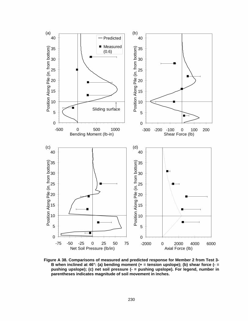
230

0

5

10

15

20

25

30

35

40


Pos

ition

Alo

ng P

ile (

in.

from

bot

tom

)

Predicted

Measured(0.6)

Sliding surface

(a)

0

5

10

15

20

25

30

35

40

-300 -200 -100 0 100 200Shear Force (lb)

Pos

ition

Alo

ng P

ile (

in.

from

bot

tom

)

(b)

0

5

10

15

20

25

30

35

40


Pos

ition

Alo

ng P

ile (

in.

from

bot

tom

)

(c)

0

5

10

15

20

25

30

35

40

-2000 0 2000 4000 6000Axial Force (lb)

Pos

ition

Alo

ng P

ile (

in.

from

bot

tom

)

(d)


231

0

5

10

15

20

25

30

35

40


Pos

ition

Alo

ng P

ile (

in.

from

bot

tom

)

Predicted

Measured(1.0)

Sliding surface

(a)

0

5

10

15

20

25

30

35

40

-300 -200 -100 0 100 200Shear Force (lb)

Pos

ition

Alo

ng P

ile (

in.

from

bot

tom

)

(b)

0

5

10

15

20

25

30

35

40


Pos

ition

Alo

ng P

ile (

in.

from

bot

tom

)

(c)

0

5

10

15

20

25

30

35

40

0 2000 4000 6000Axial Force (lb)

Pos

ition

Alo

ng P

ile (

in.

from

bot

tom

)

(d)


232

0

5

10

15

20

25

30

35


Pos

ition

Alo

ng P

ile (

in.

from

bot

tom

)

Predicted

Measured(0.03)

Sliding surface

(a)

0

5

10

15

20

25

30

35


Pos

ition

Alo

ng P

ile (

in.

from

bot

tom

)

(b)

0

5

10

15

20

25

30

35


Pos

ition

Alo

ng P

ile (

in.

from

bot

tom

)

(c)

0

5

10

15

20

25

30

35

-6000 -4000 -2000 0Axial Force (lb)

Pos

ition

Alo

ng P

ile (

in.

from

bot

tom

)

(d)


233

0

5

10

15

20

25

30


Pos

ition

Alo

ng P

ile (

in.

from

bot

tom

)

Predicted

Measured(0.05)

Sliding surface

(a)

0

5

10

15

20

25

30

-300 -150 0 150 300Shear Force (lb)

Pos

ition

Alo

ng P

ile (

in.

from

bot

tom

)

(b)

0

5

10

15

20

25

30


Pos

ition

Alo

ng P

ile (

in.

from

bot

tom

)

(c)

0

5

10

15

20

25

30


Pos

ition

Alo

ng P

ile (

in.

from

bot

tom

)

(d)


234

0

5

10

15

20

25

30


Pos

ition

Alo

ng P

ile (

in.

from

bot

tom

)

Predicted

Measured(0.2)

(a)

Sliding surface

0

5

10

15

20

25

30

-600 -300 0 300Shear Force (lb)

Pos

ition

Alo

ng P

ile (

in.

from

bot

tom

)

(b)

0

5

10

15

20

25

30


Pos

ition

Alo

ng P

ile (

in.

from

bot

tom

)

(c)

0

5

10

15

20

25

30

-6000 -4000 -2000 0 2000 4000Axial Load (lb)

Pos

ition

Alo

ng P

ile (

in.

from

bot

tom

)

(d)


235

0

5

10

15

20

25

30


Pos

ition

Alo

ng P

ile (

in.

from

bot

tom

)

Predicted

Measured(0.6)

(a)

Slidingsurface

0

5

10

15

20

25

30

-750 -500 -250 0 250 500Shear Force (lb)

Pos

ition

Alo

ng P

ile (

in.

from

bot

tom

)

(b)

0

5

10

15

20

25

30


Pos

ition

Alo

ng P

ile (

in.

from

bot

tom

)

(c)

0

5

10

15

20

25

30

-6000 -3000 0 3000Axial Force (lb)

Pos

ition

Alo

ng P

ile (

in.

from

bot

tom

)

(d)


236

0

5

10

15

20

25

30


Pos

ition

Alo

ng P

ile (

in.

from

bot

tom

)

Predicted

Measured(1.0)

Slidingsurface

(a)

0

5

10

15

20

25

30

-800 -400 0 400Shear Force (lb)

Pos

ition

Alo

ng P

ile (

in.

from

bot

tom

)

(b)

0

5

10

15

20

25

30


Pos

ition

Alo

ng P

ile (

in.

from

bot

tom

)

(c)

0

5

10

15

20

25

30

-8000 -4000 0 4000Axial Force (lb)

Pos

ition

Alo

ng P

ile (

in.

from

bot

tom

)

(d


237

Test 3-C




(in.) Sliding Depth

(in.)

30 0.2 26 12

38 0.4 26 12

40 0.45 26 14

42 0.5 26 11

43 0.7 26 14

Table A 17. Back-calculated p-, y- and t- multipliers for Test 3-C.

Pile Batter Member




238

0

5

10

15

20

25

30

35


Pos

ition

Alo

ng P

ile (

in.

from

bot

tom

)


Sliding surface

(a)

0

5

10

15

20

25

30

35


Pos

ition

Alo

ng P

ile (

in.

from

bot

tom

)

(b)

0

5

10

15

20

25

30

35


Pos

ition

Alo

ng P

ile (

in.

from

bot

tom

)

(c)

0

5

10

15

20

25

30

35

-5000 0 5000 10000Axial Force (lb)

Pos

ition

Alo

ng P

ile (

in.

from

bot

tom

)

(d)


239

0

5

10

15

20

25

30

35


Pos

ition

Alo

ng P

ile (

in.

from

bot

tom

)

Measured(0.4)

Predicted

Sliding surface

(a)

0

5

10

15

20

25

30

35

-1500 -1000 -500 0 500 1000Shear Force (lb)

Pos

ition

Alo

ng P

ile (

in.

from

bot

tom

)

(b)

0

5

10

15

20

25

30

35


Pos

ition

Alo

ng P

ile (

in.

from

bot

tom

)

(c)

0

5

10

15

20

25

30

35

-10000 -5000 0 5000 10000Axial Force (lb)

Pos

ition

Alo

ng P

ile (

in.

from

bot

tom

)

(d)


240

0

5

10

15

20

25

30

35


Pos

ition

Alo

ng P

ile (

in.

from

bot

tom

)

Measured(0.45)

Predicted

Slidingsurface

(a)

0

5

10

15

20

25

30

35

-1500 -750 0 750 1500Shear Force (lb)

Pos

ition

Alo

ng P

ile (

in.

from

bot

tom

)

(b)

0

5

10

15

20

25

30

35


Pos

ition

Alo

ng P

ile (

in.

from

bot

tom

)

(c)

0

5

10

15

20

25

30

35

-10000 0 10000 20000Axial Force (lb)

Pos

ition

Alo

ng P

ile (

in.

from

bot

tom

)

(d)


241

0

5

10

15

20

25

30

35


Pos

ition

Alo

ng P

ile (

in.

from

bot

tom

)


Slidingsurface

(a)

0

5

10

15

20

25

30

35

-1000 -500 0 500 1000Shear Force (lb)

Pos

ition

Alo

ng P

ile (

in.

from

bot

tom

)

(b)

0

5

10

15

20

25

30

35


Pos

ition

Alo

ng P

ile (

in.

from

bot

tom

)

(c)

0

5

10

15

20

25

30

35

-10000 0 10000 20000Axial Force (lb)

Pos

ition

Alo

ng P

ile (

in.

from

bot

tom

)

(d)


242

0

5

10

15

20

25

30

35


Pos

ition

Alo

ng P

ile (

in.

from

bot

tom

)

Measured(0.7)

Predicted

Sliding surface

(a)

0

5

10

15

20

25

30

35

-1000 -500 0 500 1000Shear Force (lb)

Pos

ition

Alo

ng P

ile (

in.

from

bot

tom

)

(b)

0

5

10

15

20

25

30

35


Pos

ition

Alo

ng P

ile (

in.

from

bot

tom

)

(c)

0

5

10

15

20

25

30

35

-10000 -5000 0 5000 10000Axial Force (lb)

Pos

ition

Alo

ng P

ile (

in.

from

bot

tom

)

(d)


243

0

5

10

15

20

25

30

-750 -500 -250 0 250 500 750Bending Moment (lb-in)

Pos

ition

Alo

ng P

ile (

in.

from

bot

tom

)

Predicted

Measured(0.2)

Slidingsurface

(a)

0

5

10

15

20

25

30

-300 -150 0 150Shear Force (lb)

Pos

ition

Alo

ng P

ile (

in.

from

bot

tom

)

(b)

0

5

10

15

20

25

30


Pos

ition

Alo

ng P

ile (

in.

from

bot

tom

)

0

5

10

15

20

25

30


Pos

ition

Alo

ng P

ile (

in.

from

bot

tom

)

(d)


244

0

5

10

15

20

25

30


Pos

ition

Alo

ng P

ile (

in.

from

bot

tom

)

Predicted

Measured(0.4)

Sliding surface

(a)

0

5

10

15

20

25

30

-500 -250 0Shear Force (lb)

Pos

ition

Alo

ng P

ile (

in.

from

bot

tom

)

(b)

0

5

10

15

20

25

30

-60 -30 0 30 60 90 120Net Soil Pressure (lb/in)

Pos

ition

Alo

ng P

ile (

in.

from

bot

tom

)

(c)

0

5

10

15

20

25

30

-2000 -1000 0 1000 2000 3000Axial Force (lb)

Pos

ition

Alo

ng P

ile (

in.

from

bot

tom

)

(d)


245

0

5

10

15

20

25

30


Pos

ition

Alo

ng P

ile (

in.

from

bot

tom

)

Predicted

Measured(0.45)

Sliding surface

(a)

0

5

10

15

20

25

30

-500 -250 0 250Shear Force (lb)

Pos

ition

Alo

ng P

ile (

in.

from

bot

tom

)

(b)

0

5

10

15

20

25

30


Pos

ition

Alo

ng P

ile (

in.

from

bot

tom

)

(c)

0

5

10

15

20

25

30


Pos

ition

Alo

ng P

ile (

in.

from

bot

tom

)

(d)


246

0

5

10

15

20

25

30


Pos

ition

Alo

ng P

ile (

in.

from

bot

tom

)

Predicted

Measured(0.5)

Sliding surface

(a)

0

5

10

15

20

25

30

-400 -200 0 200Shear Force (lb)

Pos

ition

Alo

ng P

ile (

in.

from

bot

tom

)

(b)

0

5

10

15

20

25

30


Pos

ition

Alo

ng P

ile (

in.

from

bot

tom

)

(c)

0

5

10

15

20

25

30


Pos

ition

Alo

ng P

ile (

in.

from

bot

tom

)

(d)


247

0

5

10

15

20

25

30


Pos

ition

Alo

ng P

ile (

in.

from

bot

tom

)

Measured(0.7)

Predicted

Slidingsurface

(a)

0

5

10

15

20

25

30

-500 -250 0 250Shear Force (lb)

Pos

ition

Alo

ng P

ile (

in.

from

bot

tom

)

(b)

0

5

10

15

20

25

30


Pos

ition

Alo

ng P

ile (

in.

from

bot

tom

)

(c)

0

5

10

15

20

25

30


Pos

ition

Alo

ng P

ile (

in.

from

bot

tom

)

(d)


248

Test 3-D

Table A 18. Test parameters used for back-analyses of pile response for Test 3-D.



(in.) Sliding Depth

(in.)

30 0.6 16 12 40 0.8 14 16 43 1 14 16 45 1.4 16 15 46 1.8 16 16

Table A 19. Back-calculated p-, y- and t- multipliers for Test 3-D.



249

0

5

10

15

20

25

30

35


Pos

ition

Alo

ng P

ile (

in.

from

bot

tom

)

Member 3(0.6)

Predicted

Member 1

Slidingsurface

(a)

0

5

10

15

20

25

30

35


Pos

ition

Alo

ng P

ile (

in.

from

bot

tom

)

(b)

0

5

10

15

20

25

30

35


Pos

ition

Alo

ng P

ile (

in.

from

bot

tom

)

(c)

0

5

10

15

20

25

30

35

-1000 0 1000 2000Axial Force (lb)

Pos

ition

Alo

ng P

ile (

in.

from

bot

tom

)

(d)

Figure A 55. Comparisons of measured and predicted response for upslope piles from Test 3-D when inclined at 30°: (a) bending moment (+ = tension upslope); (b) shear force (- = pushing upslope); (c) net soil pressure (- = pushing upslope). For legend, number in parentheses indicates magnitude of soil movement in inches. Horizontal bars indicate upper and lower bound for Member 3.

250

0

5

10

15

20

25

30

35


Pos

ition

Alo

ng P

ile (

in.

from

bot

tom

)


Member 1

Slidingsurface

(a)

0

5

10

15

20

25

30

35

-100 -50 0 50 100Shear Force (lb)

Pos

ition

Alo

ng P

ile (

in.

from

bot

tom

)

(b)

0

5

10

15

20

25

30

35


Pos

ition

Alo

ng P

ile (

in.

from

bot

tom

)

(c)

0

5

10

15

20

25

30

35

-500 0 500 1000 1500 2000Axial Force (lb)

Pos

ition

Alo

ng P

ile (

in.

from

bot

tom

)

(d)


251

0

5

10

15

20

25

30

35

-750 -500 -250 0 250 500 750Bending Moment (lb-in)

Pos

ition

Alo

ng P

ile (

in.

from

bot

tom

)


Member 1

Sliding surface

(a)

0

5

10

15

20

25

30

35

-200 -100 0 100Shear Force (lb)

Pos

ition

Alo

ng P

ile (

in.

from

bot

tom

)

(b)

0

5

10

15

20

25

30

35


Pos

ition

Alo

ng P

ile (

in.

from

bot

tom

)

(c)

0

5

10

15

20

25

30

35


Pos

ition

Alo

ng P

ile (

in.

from

bot

tom

)

(d)


252

0

5

10

15

20

25

30

35


Pos

ition

Alo

ng P

ile (

in.

from

bot

tom

)

Member 3(1.4)

Predicted

Member 1

Sliding surface

(a)

0

5

10

15

20

25

30

35


Pos

ition

Alo

ng P

ile (

in.

from

bot

tom

)

(b)

0

5

10

15

20

25

30

35


Pos

ition

Alo

ng P

ile (

in.

from

bot

tom

)

(c)

0

5

10

15

20

25

30

35

-2500 0 2500 5000Axial Force (lb)

Pos

ition

Alo

ng P

ile (

in.

from

bot

tom

)

(d)


253

0

5

10

15

20

25

30

35


Pos

ition

Alo

ng P

ile (

in.

from

bot

tom

)


Member 1

Sliding surface

(a)

0

5

10

15

20

25

30

35


Pos

ition

Alo

ng P

ile (

in.

from

bot

tom

)

(b)

0

5

10

15

20

25

30

35

-30 0 30 60Net Soil Pressure (lb/in)

Pos

ition

Alo

ng P

ile (

in.

from

bot

tom

)

(c)

0

5

10

15

20

25

30

35

-2000 0 2000 4000 6000Axial Force (lb)

Pos

ition

Alo

ng P

ile (

in.

from

bot

tom

)

(d)


254

0

5

10

15

20

25


Pos

ition

Alo

ng P

ile (

in.

from

bot

tom

)

(a)

Sliding Surface

0

5

10

15

20

25

-150 -100 -50 0 50 100 150Shear Force (lb)

Pos

ition

Alo

ng P

ile (

in.

from

bot

tom

)


Member 4

(b)

0

5

10

15

20

25


Pos

ition

Alo

ng P

ile (

in.

from

bot

tom

)

(c)

0

5

10

15

20

25

-2000 0 2000 4000Axial Force (lb)

Pos

ition

Alo

ng P

ile (

in.

from

bot

tom

)

(d)

Figure A 60. Comparisons of measured and predicted response for downslope piles from Test 3-D when inclined at 30°: (a) bending moment (+ = tension upslope); (b) shear force (- = pushing upslope); (c) net soil pressure (- = pushing upslope). For legend, number in parentheses indicates magnitude of soil movement in inches. Horizontal bars indicate upper and lower bound for Member 2.

255

0

5

10

15

20

25


Pos

ition

Alo

ng P

ile (

in.

from

bot

tom

)

Member 2(0.8)

Predicted

Member 4

(a)

Sliding surface

0

5

10

15

20

25

-400 -200 0 200Shear Force (lb)

Pos

ition

Alo

ng P

ile (

in.

from

bot

tom

)

(b)

0

5

10

15

20

25


Pos

ition

Alo

ng P

ile (

in.

from

bot

tom

)

(c)

0

5

10

15

20

25

-3000 0 3000 6000Axial Force (lb)

Pos

ition

Alo

ng P

ile (

in.

from

bot

tom

)

(d)


256

0

5

10

15

20

25


Pos

ition

Alo

ng P

ile (

in.

from

bot

tom

)

Member2 (1.0)Predicted

Member4

Sliding surface

(a)

0

5

10

15

20

25

-400 -200 0 200Shear Force (lb)

Pos

ition

Alo

ng P

ile (

in.

from

bot

tom

)

(b)

0

5

10

15

20

25


Pos

ition

Alo

ng P

ile (

in.

from

bot

tom

)

(c)

0

5

10

15

20

25

-3000 0 3000 6000 9000Axial Force (lb)

Pos

ition

Alo

ng P

ile (

in.

from

bot

tom

)

(d)


257

0

5

10

15

20

25


Pos

ition

Alo

ng P

ile (

in.

from

bot

tom

)

Measured2 (1.4)

Predicted

Member 4

Slidingsurface

(a)

0

5

10

15

20

25

-300 -200 -100 0 100 200Shear Force (lb)

Pos

ition

Alo

ng P

ile (

in.

from

bot

tom

)

(b)

0

5

10

15

20

25


Pos

ition

Alo

ng P

ile (

in.

from

bot

tom

)

(c)

0

5

10

15

20

25

-3000 0 3000 6000 9000Axial Force (lb)

Pos

ition

Alo

ng P

ile (

in.

from

bot

tom

)

(d)


258

0

5

10

15

20

25

-1500 -1000 -500 0 500 1000Bending Moment (lb-in)

Pos

ition

Alo

ng P

ile (

in.

from

bot

tom

)


Member 4

Slidingsurface

(a)

0

5

10

15

20

25

-300 -150 0 150Shear Force (lb)

Pos

ition

Alo

ng P

ile (

in.

from

bot

tom

)

(b)

0

5

10

15

20

25


Pos

ition

Alo

ng P

ile (

in.

from

bot

tom

)

(c)

0

5

10

15

20

25

-3000 0 3000 6000 9000Axial Force (lb)

Pos

ition

Alo

ng P

ile (

in.

from

bot

tom

)

(d)


259

Test 3-E

Table A 20. Test Parameters used for back-analyses of pile response for Test 3-E.



(in.) Sliding Depth

(in.) 36 0.1 14 12 40 0.25 8 10 43 0.5 13 13 44 0.9 16 16 45 1.45 14 16

Table A 21. Back-calculated p-, y- and t- multipliers for Test 3-E.



260

0

5

10

15

20

25

30

35


Pos

ition

Alo

ng P

ile (

in.

from

bot

tom

)


Member 1

Sliding surface

(a)

0

5

10

15

20

25

30

35

-75 -50 -25 0 25 50Shear Force (lb)

Pos

ition

Alo

ng P

ile (

in.

from

bot

tom

)

(b)

0

5

10

15

20

25

30

35


Pos

ition

Alo

ng P

ile (

in.

from

bot

tom

)

(c)

0

5

10

15

20

25

30

35

-1000 0 1000 2000 3000Axial Force (lb)

Pos

ition

Alo

ng P

ile (

in.

from

bot

tom

)

(d)

Figure A 65. Comparisons of measured and predicted response for upslope piles from Test 3-E when inclined at 36°: (a) bending moment (+ = tension upslope); (b) shear force (- = pushing upslope); (c) net soil pressure (- = pushing upslope). For legend, number in parentheses indicates magnitude of soil movement in inches. Horizontal bars indicate upper and lower bound for Member 3.

261

0

5

10

15

20

25

30

35


Pos

ition

Alo

ng P

ile (

in. f

rom

bot

tom

)


Member 1

Sliding surface

(a)

0

5

10

15

20

25

30

35

-40 -20 0 20 40Shear Force (lb)

Pos

ition

Alo

ng P

ile (

in.

from

bot

tom

)

(b)

0

5

10

15

20

25

30

35


Pos

ition

Alo

ng P

ile (

in.

from

bot

tom

)

(c)

0

5

10

15

20

25

30

35

-5000 0 5000 10000

Axial Force (lb)

Pos

ition

Alo

ng P

ile (

in.

from

bot

tom

)

(d)


262

0

5

10

15

20

25

30

35


Pos

ition

Alo

ng P

ile (

in.

from

bot

tom

)

Member 3(0.5)

Predicted

Member 1

Slidingsurface

(a)

0

5

10

15

20

25

30

35


Pos

ition

Alo

ng P

ile (

in.

from

bot

tom

)

2

(b)

0

5

10

15

20

25

30

35


Pos

ition

Alo

ng P

ile (

in.

from

bot

tom

)

(c)

0

5

10

15

20

25

30

35

-2000 -1000 0 1000 2000 3000Axial Force (lb)

Pos

ition

Alo

ng P

ile (

in.

from

bot

tom

)

(d)


263

0

5

10

15

20

25

30

35


Pos

ition

Alo

ng P

ile (

in.

from

bot

tom

)


Member 1

Slidingsurface

(a)

0

5

10

15

20

25

30

35

-150 -100 -50 0 50Shear Force (lb)

Pos

ition

Alo

ng P

ile (

in.

from

bot

tom

)

(b)

0

5

10

15

20

25

30

35


Pos

ition

Alo

ng P

ile (

in.

from

bot

tom

)

(c)

0

5

10

15

20

25

30

35

-2000 0 2000 4000Axial Force (lb)

Pos

ition

Alo

ng P

ile (

in.

from

bot

tom

)

(d)


264

0

5

10

15

20

25

30

35


Pos

ition

Alo

ng P

ile (

in.

from

bot

tom

)

Member 3(1.45)

Predicted

Member 1

(a)

Sliding surface

0

5

10

15

20

25

30

35

-150 -100 -50 0 50 100 150Shear Force (lb)

Pos

ition

Alo

ng P

ile (

in.

from

bot

tom

)

(b)

0

5

10

15

20

25

30

35


Pos

ition

Alo

ng P

ile (

in.

from

bot

tom

)

(c)

0

5

10

15

20

25

30

35

-2000 0 2000 4000Axial Force (lb)

Pos

ition

Alo

ng P

ile (

in.

from

bot

tom

)

(d)


265

0

5

10

15

20

25


Pos

ition

Alo

ng P

ile (

in.

from

bot

tom

)

Member 2(0.1)

Predicted

Member 4

Sliding surface

(a)

0

5

10

15

20

25

-200 -100 0 100Shear Force (lb)

Pos

ition

Alo

ng P

ile (

in.

from

bot

tom

)

(b)

0

5

10

15

20

25


Pos

ition

Alo

ng P

ile (

in.

from

bot

tom

)

(c)

0

5

10

15

20

25

-2000 -1500 -1000 -500 0Axial Force (lb)

Pos

ition

Alo

ng P

ile (

in.

from

bot

tom

)

(d)

Figure A 70. Comparisons of measured and predicted response for downslope piles from Test 3-E when inclined at 36°: (a) bending moment (+ = tension upslope); (b) shear force (- = pushing upslope); (c) net soil pressure (- = pushing upslope). For legend, number in parentheses indicates magnitude of soil movement in inches. Horizontal bars indicate upper and lower bound for Member 2.

266

0

5

10

15

20

25


Pos

ition

Alo

ng P

ile (

in.

from

bot

tom

)

Member 2(0.25)

Predicted

Member 4

Sliding surface

(a)

0

5

10

15

20

25

-200 -100 0 100Shear Force (lb)

Pos

ition

Alo

ng P

ile (

in.

from

bot

tom

)

(b)

0

5

10

15

20

25


Pos

ition

Alo

ng P

ile (

in.

from

bot

tom

)

(c)

0

5

10

15

20

25

-1000 0 1000 2000 3000Axial Force (lb)

Pos

ition

Alo

ng P

ile (

in.

from

bot

tom

)

(d)


267

0

5

10

15

20

25


Pos

ition

Alo

ng P

ile (

in.

from

bot

tom

)


Member 4

(a)

Slidingsurface

0

5

10

15

20

25

-160 -80 0 80 160Shear Force (lb)

Pos

ition

Alo

ng P

ile (

in.

from

bot

tom

)

(b)

0

5

10

15

20

25

-50 0 50Soil Pressure (lb/in)

Pos

ition

Alo

ng P

ile (

in.

from

bot

tom

)

(c)

0

5

10

15

20

25


Pos

ition

Alo

ng P

ile (

in.

from

bot

tom

)

(d)


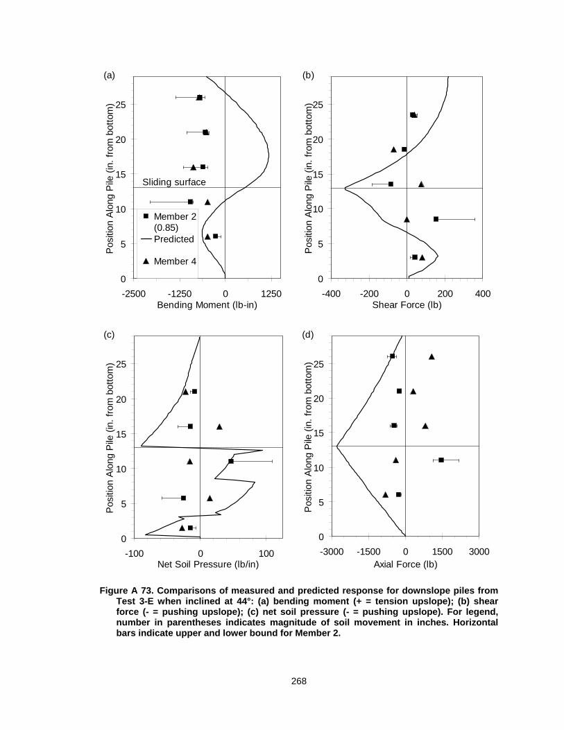
268

0

5

10

15

20

25


Pos

ition

Alo

ng P

ile (

in.

from

bot

tom

)


Member 4

Sliding surface

(a)

0

5

10

15

20

25

-400 -200 0 200 400Shear Force (lb)

Pos

ition

Alo

ng P

ile (

in.

from

bot

tom

)

(b)

0

5

10

15

20

25


Pos

ition

Alo

ng P

ile (

in.

from

bot

tom

)

(c)

0

5

10

15

20

25

-3000 -1500 0 1500 3000Axial Force (lb)

Pos

ition

Alo

ng P

ile (

in.

from

bot

tom

)

(d)


269

0

5

10

15

20

25


Pos

ition

Alo

ng P

ile (

in.

from

bot

tom

)


Member 4

(a)

Sliding surface

0

5

10

15

20

25


Pos

ition

Alo

ng P

ile (

in.

from

bot

tom

)

(b)

0

5

10

15

20

25


Pos

ition

Alo

ng P

ile (

in.

from

bot

tom

)

(c)

0

5

10

15

20

25

-4000 -2000 0 2000 4000 6000Axial Force (lb)

Pos

ition

Alo

ng P

ile (

in.

from

bot

tom

)

(d)


270

Test 3-F

Table A 22. Test parameters used for back-analyses of pile response for Test 3-F.



(in.) Sliding Depth

(in.) 34 0.25 14 15 36 0.3 13 16 40 0.8 13 16 45 1.3 13 16

Table A 23. Back-calculated p-, y- and t- multipliers for Test 3-F.

Pile Batter Member


p-multiplier y-multiplier t-multiplier Upslope 2, 3 0.25 0.65 40

Downlsope 1, 4 1.5 0.8 40

271

0

5

10

15

20

25

30

35


Pos

ition

Alo

ng P

ile (

in.

from

bot

tom

)

Member 3(0.25)

Predicted

Member 2

Sliding surface

(a)

0

5

10

15

20

25

30

35

-75 -50 -25 0 25Shear Force (lb)

Pos

ition

Alo

ng P

ile (

in.

from

bot

tom

)

(b)

0

5

10

15

20

25

30

35


Pos

ition

Alo

ng P

ile (

in.

from

bot

tom

)

(c)

0

5

10

15

20

25

30

35

0 1000 2000 3000Axial Force (lb)

Pos

ition

Alo

ng P

ile (

in.

from

bot

tom

)

(d)

Figure A 75. Comparisons of measured and predicted response for upslope piles from

Test 3-F when inclined at 34°: (a) bending moment (+ = tension upslope); (b) shear force (- = pushing upslope); (c) net soil pressure (- = pushing upslope). For legend, number in parentheses indicates magnitude of soil movement in inches. Horizontal bars indicate upper and lower bound for Member 3.

272

0

5

10

15

20

25

30

35


Pos

ition

Alo

ng P

ile (

in.

from

bot

tom

)

Member 3(0.3)

Predicted

Member 2

Sliding surface

(a)

0

5

10

15

20

25

30

35

-75 -50 -25 0 25Shear Force (lb)

Pos

ition

Alo

ng P

ile (

in.

from

bot

tom

)

(b)

0

5

10

15

20

25

30

35


Pos

ition

Alo

ng P

ile (

in.

from

bot

tom

)

(c)

0

5

10

15

20

25

30

35

0 1000 2000 3000Axial Force (lb)

Pos

ition

Alo

ng P

ile (

in.

from

bot

tom

)

(d)

Figure A 76. Comparisons of measured and predicted response for upslope piles from Test 3-F when inclined at 36°: (a) bending moment (+ = tension upslope); (b) shear force (- = pushing upslope); (c) net soil pressure (- = pushing upslope). For legend, number in parentheses indicates magnitude of soil movement in inches. Horizontal bars indicate upper and lower bound for Member 3.

273

0

5

10

15

20

25

30

35


Pos

ition

Alo

ng P

ile (

in.

from

bot

tom

)

Member 3(0.8)

Predicted

Member 2

Sliding surface

(a)

0

5

10

15

20

25

30

35

-75 -50 -25 0 25Shear Force (lb)

Pos

ition

Alo

ng P

ile (

in.

from

bot

tom

)

(b)

0

5

10

15

20

25

30

35


Pos

ition

Alo

ng P

ile (

in.

from

bot

tom

)

(c)

0

5

10

15

20

25

30

35

-1000 0 1000 2000 3000Axial Force (lb)

Pos

ition

Alo

ng P

ile (

in.

from

bot

tom

)

(d)


274

0

5

10

15

20

25

30

35


Pos

ition

Alo

ng P

ile (

in.

from

bot

tom

)

Member 3(1.25)

Predicted

Member 2

Sliding surface

(a)

0

5

10

15

20

25

30

35

-120 -90 -60 -30 0 30Shear Force (lb)

Pos

ition

Alo

ng P

ile (

in.

from

bot

tom

)

(b)

0

5

10

15

20

25

30

35


Pos

ition

Alo

ng P

ile (

in.

from

bot

tom

)

(c)

0

5

10

15

20

25

30

35

-1000 0 1000 2000 3000Axial Force (lb)

Pos

ition

Alo

ng P

ile (

in.

from

bot

tom

)

(d)


275

0

5

10

15

20

25


Pos

ition

Alo

ng P

ile (

in.

from

bot

tom

)

Member 1(0.25)

Predicted

Member 4

Slidingsurface

(a)

0

5

10

15

20

25


Pos

ition

Alo

ng P

ile (

in.

from

bot

tom

)

(b)

0

5

10

15

20

25


Pos

ition

Alo

ng P

ile (

in.

from

bot

tom

)

(c)

0

5

10

15

20

25


Pos

ition

Alo

ng P

ile (

in.

from

bot

tom

)

(d)

Figure A 79. Comparisons of measured and predicted response for downslope piles from Test 3-F when inclined at 34°: (a) bending moment (+ = tension upslope); (b) shear force (- = pushing upslope); (c) net soil pressure (- = pushing upslope). For legend, number in parentheses indicates magnitude of soil movement in inches. Horizontal bars indicate upper and lower bound for Member 1.

276

0

5

10

15

20

25


Pos

ition

Alo

ng P

ile (

in.

from

bot

tom

)

Member 1(0.3)

Predicted

Member 4

Sliding surface

(a)

0

5

10

15

20

25


Pos

ition

Alo

ng P

ile (

in.

from

bot

tom

)

(b)

0

5

10

15

20

25


Pos

ition

Alo

ng P

ile (

in.

from

bot

tom

)

(c)

0

5

10

15

20

25

-3000 -1000 1000 3000 5000Axial Force (lb)

Pos

ition

Alo

ng P

ile (

in.

from

bot

tom

)

(d)


277

0

5

10

15

20

25


Pos

ition

Alo

ng P

ile (

in.

from

bot

tom

)


Member 4

Slidingsurface

(a)

0

5

10

15

20

25

-500 -250 0 250 500 750Shear Force (lb)

Pos

ition

Alo

ng P

ile (

in.

from

bot

tom

)

(b)

0

5

10

15

20

25


Pos

ition

Alo

ng P

ile (

in.

from

bot

tom

)

(c)

0

5

10

15

20

25

-3000 0 3000 6000 9000Axial Force (lb)

Pos

ition

Alo

ng P

ile (

in.

from

bot

tom

)

(d)


278

0

5

10

15

20

25


Pos

ition

Alo

ng P

ile (

in.

from

bot

tom

)

Member 1(1.25)

Predicted

Member 4

Sliding surface

(a)

0

5

10

15

20

25


Pos

ition

Alo

ng P

ile (

in.

from

bot

tom

)

(b)

0

5

10

15

20

25


Pos

ition

Alo

ng P

ile (

in.

from

bot

tom

)

(c)

0

5

10

15

20

25

-5000 0 5000 10000Axial Force (lb)

Pos

ition

Alo

ng P

ile (

in.

from

bot

tom

)

(d)


279

Test 4-A




(in.) Sliding Depth

(in.) 30 0.2 10 12 36 0.3 12 16 38 0.5 12 16



Upslope 1 0.3 0.9 40 Downlsope 2 1.2 1 40

280

0

5

10

15

20

25

30


Pos

ition

Alo

ng P

ile (

in.

from

bot

tom

)

Measured(0.2)

Predicted

Slidingsurface

(a)

0

5

10

15

20

25

30

-40 -20 0 20 40Shear Force (lb)

Pos

ition

Alo

ng P

ile (

in.

from

bot

tom

)

(b)

0

5

10

15

20

25

30


Pos

ition

Alo

ng P

ile (

in.

from

bot

tom

)

(c)

0

5

10

15

20

25

30

-500 0 500 1000 1500 2000Axial Force (lb)

Pos

ition

Alo

ng P

ile (

in.

from

bot

tom

)

(d)


281

0

5

10

15

20

25

30


Pos

ition

Alo

ng P

ile (

in.

from

bot

tom

)

Measured(0.3)

Predicted

Slidingsurface

(a)

0

5

10

15

20

25

30

-75 -50 -25 0 25 50 75Shear Force (lb)

Pos

ition

Alo

ng P

ile (

in.

from

bot

tom

)

(b)

0

5

10

15

20

25

30


Pos

ition

Alo

ng P

ile (

in.

from

bot

tom

)

(c)

0

5

10

15

20

25

30

-1000 0 1000 2000Axial Force (lb)

Pos

ition

Alo

ng P

ile (

in.

from

bot

tom

)

(d)


282

0

5

10

15

20

25

30


Pos

ition

Alo

ng P

ile (

in.

from

bot

tom

)

Measured(0.5)

Predicted

Sliding surface

(a)

0

5

10

15

20

25

30


Pos

ition

Alo

ng P

ile (

in.

from

bot

tom

)

(b)

0

5

10

15

20

25

30


Pos

ition

Alo

ng P

ile (

in.

from

bot

tom

)

(c)

0

5

10

15

20

25

30

-1000 0 1000 2000 3000Axial Force (lb)

Pos

ition

Alo

ng P

ile (

in.

from

bot

tom

)

(d)


283

0

5

10

15

20

25


Pos

ition

Alo

ng P

ile (

in.

from

bot

tom

)

Predicted

Measured(0.2)

Slidingsurface

(a)

0

5

10

15

20

25

-100 -50 0 50 100Shear Force (lb)

Pos

ition

Alo

ng P

ile (

in.

from

bot

tom

)

(b)

0

5

10

15

20

25


Pos

ition

Alo

ng P

ile (

in.

from

bot

tom

)

(c)

0

5

10

15

20

25

-2000 -1000 0 1000Axial Force (lb)

Pos

ition

Alo

ng P

ile (

in.

from

bot

tom

)

(c)


284

0

5

10

15

20

25

-800 0Bending Moment (lb-in)

Pos

ition

Alo

ng P

ile (

in.

from

bot

tom

)

Predicted

Measured(0.3)

Failure surface

(a)

0

5

10

15

20

25

-400 -200 0 200 400Shear Force (lb)

Pos

ition

Alo

ng P

ile (

in.

from

bot

tom

)

(b)

0

5

10

15

20

25


Pos

ition

Alo

ng P

ile (

in.

from

bot

tom

)

(c)

0

5

10

15

20

25


Pos

ition

Alo

ng P

ile (

in.

from

bot

tom

)

(d)


285

0

5

10

15

20

25


Pos

ition

Alo

ng P

ile (

in.

from

bot

tom

)

Predicted

Measured(0.5)

Sliding surface

(a)

0

5

10

15

20

25

-400 -200 0 200Shear Force (lb)

Pos

ition

Alo

ng P

ile (

in.

from

bot

tom

)

(b)

0

5

10

15

20

25


Pos

ition

Alo

ng P

ile (

in.

from

bot

tom

)

(c)

0

5

10

15

20

25

-4000 -2000 0 2000 4000Axial Force (lb)

Pos

ition

Alo

ng P

ile (

in.

from

bot

tom

)

(d)


286

Test 4-B




(in.) Sliding Depth

(in.)

41 0.1 14 12 42 0.25 12 12 43 0.7 18 12


Pile Batter Member




287

0

5

10

15

20

25

30


Pos

ition

Alo

ng P

ile (

in.

from

bot

tom

)

Measured(0.1)

Predicted

Sliding surface

(a)

0

5

10

15

20

25

30


Pos

ition

Alo

ng P

ile (

in.

from

bot

tom

)

(b)

0

5

10

15

20

25

30


Pos

ition

Alo

ng P

ile (

in.

from

bot

tom

)

(c)

0

5

10

15

20

25

30

0 500 1000 1500Axial Force (lb)

Pos

ition

Alo

ng P

ile (

in.

from

bot

tom

)

(d)

Figure A 89. Comparisons of measured and predicted response for Member 3 from Test 4-

B when inclined at 41°: (a) bending moment (+ = tension upslope); (b) shear force (- = pushing upslope); (c) net soil pressure (- = pushing upslope). For legend, number in parentheses indicates magnitude of soil movement in inches.

288

0

5

10

15

20

25

30


Pos

ition

Alo

ng P

ile (

in.

from

bot

tom

)

Measured(0.25)

Predicted

Slidingsurface

(a)

0

5

10

15

20

25

30


Pos

ition

Alo

ng P

ile (

in.

from

bot

tom

)

Measured(0.25)

Predicted

Slidingsurface

(a)

0

5

10

15

20

25

30


Pos

ition

Alo

ng P

ile (

in.

from

bot

tom

)

(c)

0

5

10

15

20

25

30

0 500 1000 1500 2000Axial Force (lb)

Pos

ition

Alo

ng P

ile (

in.

from

bot

tom

)

(d)


289

0

5

10

15

20

25

30


Pos

ition

Alo

ng P

ile (

in.

from

bot

tom

)

Measured(0.7)

Predicted

Slidingsurface

(a)

0

5

10

15

20

25

30

-400 -200 0 200 400Shear Force (lb)

Pos

ition

Alo

ng P

ile (

in.

from

bot

tom

)

(b)

0

5

10

15

20

25

30


Pos

ition

Alo

ng P

ile (

in.

from

bot

tom

)

(c)

0

5

10

15

20

25

30

-2000 0 2000 4000 6000 8000Axial Force (lb)

Pos

ition

Alo

ng P

ile (

in.

from

bot

tom

)

(d)


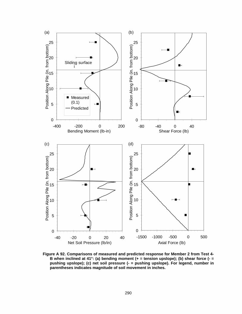
290

0

5

10

15

20

25


Pos

ition

Alo

ng P

ile (

in.

from

bot

tom

)

Measured(0.1)

Predicted

Sliding surface

(a)

0

5

10

15

20

25


Pos

ition

Alo

ng P

ile (

in.

from

bot

tom

)

(b)

0

5

10

15

20

25


Pos

ition

Alo

ng P

ile (

in.

from

bot

tom

)

(c)

0

5

10

15

20

25

-1500 -1000 -500 0 500

Axial Force (lb)

Pos

ition

Alo

ng P

ile (

in.

from

bot

tom

)

(d)


291

0

5

10

15

20

25


Pos

ition

Alo

ng P

ile (

in.

from

bot

tom

)

Measured(0.25)

Predicted

Sliding surface

(a)

0

5

10

15

20

25

-150 -100 -50 0 50 100Shear Force (lb)

Pos

ition

Alo

ng P

ile (

in.

from

bot

tom

)

(b)

0

5

10

15

20

25


Pos

ition

Alo

ng P

ile (

in.

from

bot

tom

)

(c)

0

5

10

15

20

25


Pos

ition

Alo

ng P

ile (

in.

from

bot

tom

)

(d)


292

0

5

10

15

20

25


Pos

ition

Alo

ng P

ile (

in.

from

bot

tom

)

Measured(0.7)

Predicted

Sliding surface

(a)

0

5

10

15

20

25

-150 -75 0 75 150Shear Force (lb)

Pos

ition

Alo

ng P

ile (

in.

from

bot

tom

)

(b)

0

5

10

15

20

25


Pos

ition

Alo

ng P

ile (

in.

from

bot

tom

)

(c)

0

5

10

15

20

25

-2500 -1500 -500 500 1500Axial Force (lb)

Pos

ition

Alo

ng P

ile (

in.

from

bot

tom

)

(d)


293

Test 4-C




(in.) Sliding Depth

(in.) 30 0.1 14 11 40 0.25 14 11 44 0.3 12 13 46 0.5 18 18 47 1 20 20

Table A 29. Back-calculated p-, y- and t- multipliers for Test 4-C.



294

0

5

10

15

20

25

30

35


Pos

ition

Alo

ng P

ile (

in.

from

bot

tom

)

Member 1(0.1)

Predicted

Member 3

Sliding surface

(a)

0

5

10

15

20

25

30

35


Pos

ition

Alo

ng P

ile (

in.

from

bot

tom

)

(b)

0

5

10

15

20

25

30

35


Pos

ition

Alo

ng P

ile (

in.

from

bot

tom

)

(c)

0

5

10

15

20

25

30

35

-1000 0 1000 2000 3000Axial Force (lb)

Pos

ition

Alo

ng P

ile (

in.

from

bot

tom

)

(d)

Figure A 95. Comparisons of measured and predicted response for upslope piles from Test 4-C when inclined at 30°: (a) bending moment (+ = tension upslope); (b) shear force (- = pushing upslope); (c) net soil pressure (- = pushing upslope). For legend, number in parentheses indicates magnitude of soil movement in inches. Horizontal bars indicate upper and lower bound for Member 1.

295

0

5

10

15

20

25

30

35


Pos

ition

Alo

ng P

ile (

in.

from

bot

tom

)

Member 1(0.25)

Predicted

Member 3

Sliding surface

(a)

0

5

10

15

20

25

30

35


Pos

ition

Alo

ng P

ile (

in.

from

bot

tom

)

(b)

0

5

10

15

20

25

30

35


Pos

ition

Alo

ng P

ile (

in.

from

bot

tom

)

(c)

0

5

10

15

20

25

30

35

-2000 0 2000 4000 6000Axial Force (lb)

Pos

ition

Alo

ng P

ile (

in.

from

bot

tom

)

(d)


296

0

5

10

15

20

25

30

35


Pos

ition

Alo

ng P

ile (

in.

from

bot

tom

)

Member 1(0.3)

Predicted

Member 3

(a)

Sliding surface

0

5

10

15

20

25

30

35

-200 -100 0 100 200Shear Force (lb)

Pos

ition

Alo

ng P

ile (

in.

from

bot

tom

)

(b)

0

5

10

15

20

25

30

35


Pos

ition

Alo

ng P

ile (

in.

from

bot

tom

)

(c)

0

5

10

15

20

25

30

35

0 5000 10000 15000Axial Force (lb)

Pos

ition

Alo

ng P

ile (

in.

from

bot

tom

)

(d)


297

0

5

10

15

20

25

30

35


Pos

ition

Alo

ng P

ile (

in.

from

bot

tom

)

Member 1(0.45)

Predicted

Member 3

Sliding surface

(a)

0

5

10

15

20

25

30

35

-300 -200 -100 0 100 200Shear Force (lb)

Pos

ition

Alo

ng P

ile (

in.

from

bot

tom

)

(b)

0

5

10

15

20

25

30

35


Pos

ition

Alo

ng P

ile (

in.

from

bot

tom

)

(c)

0

5

10

15

20

25

30

35


Pos

ition

Alo

ng P

ile (

in.

from

bot

tom

)

(d)


298

0

5

10

15

20

25

30

35


Pos

ition

Alo

ng P

ile (

in.

from

bot

tom

)


Member 3

Sliding surface

(a)

0

5

10

15

20

25

30

35

-400 -200 0 200Shear Force (lb)

Pos

ition

Alo

ng P

ile (

in.

from

bot

tom

)

(b)

0

5

10

15

20

25

30

35


Pos

ition

Alo

ng P

ile (

in.

from

bot

tom

)

(c)

0

5

10

15

20

25

30

35

0 5000 10000 15000Axial Force (lb)

Pos

ition

Alo

ng P

ile (

in.

from

bot

tom

)

(d)


299

0

5

10

15

20

25


Pos

ition

Alo

ng P

ile (

in.

from

bot

tom

)

(a)

Sliding surface

0

5

10

15

20

25


Pos

ition

Alo

ng P

ile (

in.

from

bot

tom

)


Member 4

(b)

0

5

10

15

20

25


Pos

ition

Alo

ng P

ile (

in.

from

bot

tom

)

(c)

0

5

10

15

20

25

-2000 -1000 0 1000Axial Force (lb)

Pos

ition

Alo

ng P

ile (

in.

from

bot

tom

)

(d)

Figure A 100. Comparisons of measured and predicted response for downslope piles from Test 4-C when inclined at 30°: (a) bending moment (+ = tension upslope); (b) shear force (- = pushing upslope); (c) net soil pressure (- = pushing upslope). For legend, number in parentheses indicates magnitude of soil movement in inches. Horizontal bars indicate upper and lower bound for Member 2.

300

0

5

10

15

20

25


Pos

ition

Alo

ng P

ile (

in.

from

bot

tom

)

Sliding surface

(a)

0

5

10

15

20

25


Pos

ition

Alo

ng P

ile (

in.

from

bot

tom

)

Member 2(0.25)

Predicted

Member 4

(b)

0

5

10

15

20

25


Pos

ition

Alo

ng P

ile (

in.

from

bot

tom

)

(c)

0

5

10

15

20

25

-2000 -1000 0 1000Axial Force (lb)

Pos

ition

Alo

ng P

ile (

in.

from

bot

tom

)

(d)


301

0

5

10

15

20

25


Pos

ition

Alo

ng P

ile (

in.

from

bot

tom

)


Member 4

Sliding surface

(a)

0

5

10

15

20

25

-200 -100 0 100 200Shear Force (lb)

Pos

ition

Alo

ng P

ile (

in.

from

bot

tom

)

(b)

0

5

10

15

20

25


Pos

ition

Alo

ng P

ile (

in.

from

bot

tom

)

(c)

0

5

10

15

20

25


Pos

ition

Alo

ng P

ile (

in.

from

bot

tom

)

(d)


302

0

5

10

15

20

25


Pos

ition

Alo

ng P

ile (

in.

from

bot

tom

)

(a)

Sliding surface

0

5

10

15

20

25

-500 -250 0 250Shear Force (lb)

Pos

ition

Alo

ng P

ile (

in.

from

bot

tom

)


Member 4

(b)

0

5

10

15

20

25


Pos

ition

Alo

ng P

ile (

in.

from

bot

tom

)

(c)

0

5

10

15

20

25


Pos

ition

Alo

ng P

ile (

in. f

rom

bot

tom

)

(d)


303

0

5

10

15

20

25


Pos

ition

Alo

ng P

ile (

in.

from

bot

tom

)

Sliding surface

(a)

0

5

10

15

20

25


Pos

ition

Alo

ng P

ile (

in.

from

bot

tom

)


Member 4

(b)

0

5

10

15

20

25


Pos

ition

Alo

ng P

ile (

in.

from

bot

tom

)

(c)

0

5

10

15

20

25


Pos

ition

Alo

ng P

ile (

in.

from

bot

tom

)

(d)


response of micropiles in earth slopes from large …

Documents