Retail Store Scheduling for Profit

Nicolas Chapadosa, Marc Joliveaub, Pierre L’Ecuyera, Louis-Martin Rousseaub

aUniversité de Montréal, Montréal, CanadabÉcole Polytechnique de Montréal, Montréal, Canada

Abstract

In spite of its tremendous economic significance, the problem of sales staff schedule optimizationfor retail stores has received relatively scant attention. Current approaches typically attempt tominimize payroll costs by closely fitting a staffing curve derived from exogenous sales forecasts,oblivious to the ability of additional staff to (sometimes) positively impact sales. In contrast, thispaper frames the retail scheduling problem in terms of operating profit maximization, explicitlyrecognizing the dual role of sales employees as sources of revenues as well as generators of op-erating costs. We introduce a flexible stochastic model of retail store sales, estimated from store-specific historical data, that can account for the impact of all known sales drivers, including thenumber of scheduled staff, and provide an accurate sales forecast at a high intra-day resolution.We also present solution techniques based on mixed-integer (MIP) and constraint programming(CP) to efficiently solve the complex mixed integer non-linear scheduling (MINLP) problem witha profit-maximization objective. The proposed approach allows solving full weekly schedules tooptimality, or near-optimality with a very small gap. On a case-study with a medium-sized retailchain, this integrated forecasting–scheduling methodology yields significant projected net profitincreases on the order of 2-3% compared to baseline schedules.

Keywords: Shift Scheduling, Constraint Programming, Mixed Integer Programming,Non-Identical Workforce, Statistical Forecasting, Retail

1. Introduction

The retail sector accounts for a major fraction of the world’s developed economies. In theUnited States, retail sales represented about $3.9 trillion in 2010, over 25% of GDP, employingmore than 14M people at some $300B annual payroll costs (U.S. Census Bureau, 2011). Giventhese figures, it stands to reason that effective sales staff scheduling should be of critical im-portance to the profitable operations of a retail store, since staffing costs typically represent thesecond largest expense after the cost of goods sold (Ton, 2009): as a result, all efficiencies com-ing from better workforce deployment translate into an implicit margin expansion for the retailer,which immediately accrues to the bottom line.

Email addresses: chapados@iro.umontreal.ca (Nicolas Chapados), marc.joliveau@gmail.com(Marc Joliveau), lecuyer@iro.umontreal.ca (Pierre L’Ecuyer),louis-martin.rousseau@polymtl.ca (Louis-Martin Rousseau)

Preprint submitted to Elsevier November 7, 2013

The best retailers today rely on a staff schedule construction process that involves a decom-position into three steps (Netessine et al., 2010). First, the future sales over the planning horizonare forecasted, usually a few weeks to one month ahead at a 15- to 60-minute resolution. Second,this forecast is converted into labor requirements using so-called “labor standards” establishedby the business (e.g., every $100 in predicted sales during a given 15-minute period requires anadditional salesperson that should be working during that period). Finally, work schedules areoptimized in a way that attempts to match those labor requirements as snugly as possible, whilemeeting other business and regulatory constraints (e.g., one may have that an employee cannotbe asked to come to work for less than three consecutive hours or for more than eight hours intotal, must have breaks that follow certain rules, etc.).

It may be somewhat unsettling that nowhere does this process acknowledge, explicitly or tac-itly, that in many retail circumstances, salespeople actively contribute to revenue by doing theirjob well—advising an extra belt with those trousers, or these lovely earrings with that necklace—and not only represent a salary cost item to store operations. In other words, the presence of anadditional staff working at the right time drives up expected sales, a crucial dynamics ignoredwhen sales forecast tranquilly descends “from above”.

This paper, in contrast, formalizes the retail staff scheduling problem by formulating it asone of expected net operating profit maximization. It introduces a modeling decomposition thatallows representing the expected sales during a time period as a function of the number of sales-persons working, thereby capturing the impact of varying staffing hypotheses on the expectedsales. The profit-maximizing labor requirements are obtained, for a given time period, as thenumber of employees beyond which the marginal payroll cost exceed the marginal revenue gainfrom having an additional staff working. Finally, it introduces new solution techniques that areable to capture the profit maximization aspects of the problem. On a case-study with a medium-sized Canadian clothing and apparel chain, this integrated forecasting–scheduling methodologyyields significant projected net profit increases on the order of 2 to 3% with respect to baselineschedules.

Given the retail industry’s overall economic significance, the impact of staffing decisions hasreceived some attention in the literature, albeit perhaps not any commensurate with the gainsthat are to be expected from improved planning. Thompson (1995) proposed a scheduling modelthat takes into accounts a linear estimate of the marginal benefit of having additional employees,but not accounting for understaffing costs. Lam et al. (1998) and Perdikaki et al. (2012) haveshown that store revenues are causally and positively related to staffing levels, opening the doorto staffing rules based on sales forecasts. Moreover, using data from a large retailer, Ton (2009)finds that increasing the amount of labor at a store is associated with an increase in profitabilitythrough its impact on conformance quality but, surprisingly, not its impact on service quality.Mani et al. (2011) find systematic understaffing during peak hours in a study with a large retailchain, using a structural estimation technique to estimate the contribution of labor to sales. Ad-ditionally, in what is probably the most potent case to date for improving scheduling practices,Netessine et al. (2010) find—with another large retailer—strong cross-sectional association be-tween labor practices at different stores and basket values, and observe in their examples thatsmall improvements in employee scheduling and schedule execution can result in a 3% salesincrease for a moderate (or zero) cost.

Perhaps the contribution closest in flavor to what we suggest in this paper comes from thework of Kabak et al. (2008): similarly to the present paper, these authors introduce a two-stageapproach to retail workforce scheduling based on a statistical forecasting model of sales incorpo-rating an explicit labor effect. The profit-maximizing number of salespeople under this model is

2

then computed to obtain the desired hourly staffing levels in the store, assuming workforce costhomogeneity. This is followed by a optimization phase, which assigns individual employees toa set of pre-existing shifts. The approach is then validated through simulation to demonstrate itseffectiveness on a Turkish apparel store.

As we show later, our paper extends this approach by suggesting the use of complete salescurves within the schedule optimization stage, better reflecting the uncertainty surrounding thesales response model (which often exhibits a rather flat shape around the optimal number of sales-people), and easily allows optimizing schedules with non-homogenous staff costs. To achievethis goal, we first propose a stochastic model of retail store sales in terms of a revenue decompo-sition that is particularly amenable to robust and modular modeling. This decomposition allowsto obtain an accurate 15-minute-resolution forecast of sales, conditional on any desired determi-nant, opening the path to operating profit maximization.

Furthermore, in contrast to Kabak et al. (2008), the proposed schedule optimization does notuse a set of predefined shifts, but rather builds those that, while meeting labor and union regula-tions, allow to maximize profit. The main difficulty is to efficiently combine two distinct sets ofobjectives and constraints: those of the retailer, defined in terms of the number of working em-ployees in each time period, and those of the workers, defined in terms of the “friendliness” ofthe working shifts assigned to them. We formulate the profit-maximization problem as a mixedinteger non-linear problem (MINLP) where the decision variables specify the work status (work-ing, break, lunch, rest) of each employee, and we examine two ways of solving this problem.The first approach linearizes the problem and turns it into a mixed integer program (MIP), whichis then solved either directly or approximately using piecewise linear functions. The second ap-proach expresses the original MINLP as a constraint program (CP), which is solved directly. Itprovides better performance, especially on larger problems. The proposed problem formulationsare based on the use of a regular language to specify the admissibility of shifts with respect tounion agreements. Schedules are constructed both over a day and a week.

The rest is organized as follows. In Section 2 we formulate the problem, setting forth overallschedule construction objectives. In Section 3, we explain the stochastic models we developedfor sub-hour sales forecasts, and we evaluate the forecasting ability of these models on out-of-sample sales at several locations of a mid-sized clothing and apparel chain of retail stores. Wecontinue in Section 4 with two scheduling problem formulations, one as a MIP and the other asa CP, whose solutions are employee schedules that maximize expected profits, over a day andover a week (as shown in Section 5). Section 6 concludes. This paper extends work previouslypresented by Chapados et al. (2011).

2. Problem Formulation

Here we present an overview of the proposed approaches. The global schedule constructionprocess has two main steps, summarized in Figure 1:

1. Analyzing the historical workforce sales performance to construct a stochastic model ofstore behavior and to build sales curves, which give the expected sales at each store foreach time period, as a function of the number of staffs assigned to sales during that period.

2. Using these sales curves to construct admissible work schedules, for the employees, thatmaximize the expected profit.

3

!"#$%&'()$*"%+

,$$-#.&!*/$01#$%

2&3+$4%&!(#0&56(#14$7

86$)"9$&:);*$&<&3+$4

!"#$%&=1)6$%

!+()$&>)"?*&'()$*"%+

@3: =:AB"*+ 8CC)(BD

E FC$)"GH9&I(1)%E !+"JE K$91#"G(H%

Figure 1: Overview of the proposed methodology to address the problem of retail scheduling for profit.

2.1. Forecasting Sales as a Function of Staffing

Each sales curve provides a functional characterization of how the expected sales at a givenstore and time period are impacted by varying the staffing. A classical staffing demand curve, incontrast, indicates the desired number of employees at a given store, for each time period.

As outlined earlier and in Fig. 1, we model store sales through a decomposition into twosimpler quantities: (i) the number of items sold during a time period, and (ii) the average priceper item. Of course, sales could be forecast without such a decomposition, by applying standardstatistical time series approaches directly. But at the high intra-day resolutions (15-minute pe-riods) that we are considering, we found forecasts based on the decomposition to be markedlymore accurate than standard time series models having similar parametric complexity, not onlyin expectation but with respect to the whole distribution as well.

An important driving factor affecting the number of items sold is the in-store traffic, of whichwe require a precise forecast at a high intra-day resolution over the entire planning horizon,accounting for all known explanatory variables and capable of yielding sensible forecasts forstores for which little amounts of historical data are available. To this end, we introduce a trafficforecasting methodology that allows sharing statistical power across multiple locations (for achain of stores), yet allowing store-specific effects to be accurately handled.

To forecast sales, a key aspect of our contribution is the ability to parsimoniously model thejoint distribution between the two factors in the decomposition; to achieve this, we require amodel of the full posterior distribution of the number of items sold during a time period, condi-tional on the known sales drivers. This distribution exhibits significantly higher dispersion than aconditional Poisson, and a standard Poisson Generalized Linear Model (McCullagh and Nelder,1989)—which linearly relates the intensity of a conditional Poisson random variable to a setof covariates—proves insufficient for the purpose. We adapt the statistical technique of ordinalregression to obtain an accurate estimator of the posterior distribution of the number of itemssold.

The aforementioned decomposition is related to one often used by retail practitioners (e.g., Lamet al. 2001) wherein sales during a given period are written as the product of three factors: thenumber of shoppers in the store during the period, the conversion rate (how many shoppers be-

4

come buyers during that period), and the average basket (given that a shopper buys, how muchdoes s/he buy on average). However, this conventional decomposition is very sensitive to havinga precise measure of the number of shoppers in the store at any time—an information that manyretailers cannot measure precisely, or do not have at all.

A “demand curve” can be obtained from the sales curve by subtracting from the latter thewage cost incurred at each staffing level—yielding the profit curve—and finding, on the profitcurve for each store/time-period pair, the staffing that maximizes profit. This demand curve isoften useful for management purposes, providing a concise and interpretable summary of howmany employees “should” be working at any particular time. As mentioned previously thistype of optimal staffing for profit maximization is studied by Kabak et al. (2008) and also byKoole and Pot (2011) in the context of call centers where successful calls can bring revenue.However, as we show in Section 4, it is generally preferable to incorporate the sales curvesdirectly into the mathematical program that constructs the schedules, rather than trying to fit thedemand curve. This overcomes two limitations of traditional demand curves. Firstly, it allowstrue staff costs to be accounted for, at the individual employee level, allowing to dispense with acost homogeneity assumption. Secondly, it frequently happens that the profit curve is fairly flataround its maximum, in which case there is a large confidence band around the “truly optimal”number of employees; this allows for more flexibility during the scheduling process to producebetter schedules with only minor impact on the cost.

2.2. Scheduling for profit

In the retail store context, finding the optimal number of salespersons for each time period(the optimal staffing) is not sufficient, because there is generally no way to match these optimalnumbers exactly given the various constraints on the admissible shifts of employees. We couldthink of a two-stage approach that computes the optimal staffing in a first stage and then finds aset of admissible shifts that cover these required staffings, say by having a number of salespersonslarger or equal to the optimal number in each time period, at minimal cost. But such a procedureis generally suboptimal, as illustrated for example in Avramidis et al. (2010) in the context ofwork schedule construction for telephone call centers.

Here we solve the optimization problem in a single stage. The decision variables select a setof admissible working shifts, one for each employee, over the considered time horizon (one dayor one week, for example). The objective is to maximize the total expected profit, rather thanmerely minimizing salary costs under staffing constraints as usually done. That is, we recognizeexplicitly the dual role played by employees, who generate costs from their salaries but alsorevenues by driving up sales. This gives a novel problem formulation.

In the objective, the expected revenue as a function of the number of working employees, foreach time period of each day, is given by the sales curves, which are generally nonlinear, andthese expected revenues are added over the considered time horizon. The cost of each shift isassumed to be decomposable as a sum of costs over the time periods it covers, where the costover a time period depends on the day, the period, and the activity performed over that period.These costs are added up over all selected shifts, and subtracted from the total expected revenues.

This gives an integer programming problem with a nonlinear objective. The nonlinearity canbe handled by various techniques, such as extending the formulation by using boolean variablesfor every possible number of working employees in each period, approximating the sales curveswith piecewise linear functions, and modeling the nonlinear objective directly with a constraintprogram (see Section 4 for the details).

5

Table 1: Summary statistics of the data used in the case studies: the traffic refers to the number of clients entering thestore as measured by people counters and the staff-hours refers to the staffing levels historically scheduled for the storesduring the period covered.

Daily Traffic (persons) Daily Sales (C$) Daily Items Sold Daily Staff-HoursAvg Std. Dev. Avg Std. Dev. Avg Std. Dev. Avg Std. Dev.

Smallest store 199 77 2486 1560 29 20 19 5.6Average store 402 299 4329 2865 54 49 26 8.1Largest store 955 681 8494 5891 163 129 42 8.5

The constraints are of two kinds. Some address operational issues of employers, such asimposing a minimal number of working employees at any given time, constraints on the numberof full-time and part-time employees, and operating hours of the store. Other constraints dealwith union regulations or labor law, such as minimum and maximum number of hours of workper day for an employee, minimum and maximum number of hours of work per week, breakand meal placement regulations, minimum rest time (delay) between successive shifts for anemployee, etc. Each shift specifies a sequence of activities over the entire time horizon (e.g., aday or a week). In our formulation, employees can have different availabilities, but are assumedhomogenous in terms of selling efficiency.

2.3. Data for the Case study and Experimentation Context

The data used for our case study was provided by a medium-sized chain of upscale clothingand apparel retail stores. It comes from 15 stores, located in major Canadian cities, which obeynormal retail opening hours and sales cycle, including increased holiday activity and occasionalpromotional events, such as a mid-year sale and an after-Christmas sale. Stores are of two types:regular “signature” stores in standard shopping locations such as malls, and discount outlets,which exhibit substantially higher volume.

All stores are open seven days a week, with varying hours per day and per store; they areclosed only a small number of days per year on major holidays (Christmas, New Year, Easter). Atotal of 20 months of historical data was used, covering the January 2009–August-2010 period.For the purpose of estimating and evaluating the statistical forecasting models, a total of 8038store–days and 167,725 store–intra-day (30-minute) intervals were used. The available trafficdata was aggregated by 30-minute intervals, so we were able to construct sales curves for thoseintervals. On the other hand, the work schedules are defined based on 15-minute time intervals(the breaks last 15 minutes, for example). So for the scheduling, each 30-minute period wassplit in two 15-minute intervals with the same sales curve. To evaluate the schedule optimiza-tion methods, the 5089 store–days covering the latter portion of the data were used. Summarystatistics of the average traffic, sales, items sold, and historical staffing are shown in Table 1.Confidentiality agreements preclude from giving additional details.

3. Stochastic Modeling and Forecasting for Sales Curves Construction

3.1. Model Overview and Decomposition of Expected Sales

In this section, we develop stochastic models to construct the sales curves. For this, we de-compose the expected sales in any given time period as the expectation of the product of thenumber of items sold by the expected average price per item conditional on the first number.

6

Then we develop a stochastic model for the cumulative distribution function (cdf) of the numberof items sold as a function of the number of working employees on the floor, the estimated in-store traffic (or traffic proxy), and certain explanatory variables that account for seasonal effectsand special events. This model uses ordinal regression with cubic spline basis functions. Theestimated daily in-store traffic is modeled in log scale by a mixed-effects linear model, whosefixed effects are indicators that account for the month of the year, day of the week, interactions,and special events, and whose residuals follow a SARMA process. This estimated traffic is as-sumed to be distributed across opening hours of the day according to a multinomial distribution,estimated by multinomial regression. The overall model is summarized on the left of Figure 1.Sections 3.3 to 3.5 detail the submodels for the traffic proxy, the sales volume, and the condi-tional average item price, respectively. Reports on experimental results and validation are givenat the same time.

Simple ways of measuring the in-store traffic in a given time period could be by countingthe number of people entering the store during that period, or perhaps by the average number ofpeople in the store during that period. However, in practical settings, this type of informationis often unavailable, and one must rely on some indirect measure of store activity which weshall call a traffic proxy. In our case study, each store was equipped with people counters thatregister a “tick” each time a customer enters or leaves the store (the device does not distinguishthe direction), and simply count the number of ticks in each period. This recorded data does nottell precisely how many people are present in the store at any given time, or how many entered ina given time period, but nonetheless correlates well with store activity and was the best availableinformation in our case. Our traffic proxy was thus the “tick count” within each given timeperiod.

We consider j∗ stores indexed by j, over d∗ days indexed by d. Each day is divided in t∗(d, j)time periods indexed by t (the number of time periods generally depends on the day of the weekand on the store). For period t of day d in store j, let ywd,t,j be the number of employees assignedto sales on the floor (the selling employees), Td,t,j denote the traffic proxy, Xd,t,j a vector ofselected explanatory variables such as calendar regressors (time of the day, day of the week,month of the year) and indicators for special events, Vd,t,j the number of items sold (the salesvolume), Pd,t,j the average price per item, and Rd,t,j = Vd,t,jPd,t,j the total amount of sales.The number ywd,t,j of selling employees excludes the employees that (we assume) have no directimpact in turning shoppers into buyers; for instance cashiers that do not directly assist customerson the floor and employees tasked with replenishing shelves, as well as those on break. In thispaper, when scheduling the employees, we assume that there is only one type of work activity:each considered employee is assigned to sales. That is, we do not consider the situation where anemployee works on the floor for some periods and as a cashier or something else on other periods.To cover this type of situation we could extend our framework to a multi-activity setting, whichwould make the resolution more complicated (but still feasible).

The sales curves express the expected sales rd,t,j(y) = E[Rd,t,j | ywd,t,j = y] for period t ofday d in store j as a function of the number y of selling employees in the store for that period.To estimate the sales curves, we decompose the expectation as follows (the dependence of each

7

term on the deterministic explanatory variables Xd,t,j is implicit):

rd,t,j(y) = E[E[Rd,t,j | Td,t,j , ywd,t,j = y]]

= E[E[Vd,t,j E[Pd,t,j | Vd,t,j ] | Td,t,j , ywd,t,j = y]]

=

∞∑v=0

v E[P(Vd,t,j = v | Td,t,j , ywd,t,j = y)]E[Pd,t,j | Vd,t,j = v]. (1)

We shall construct separate models for the two expectations that appear in (1): the expected con-ditional probability (the conditional distribution of the volume) and the expected average priceper item as a function of the volume. The first expectation is with respect to Td,t,j , so we needa model for this random variable, and also for the conditional probability inside the expectation.The reason for introducing such a decomposition is that it reduces significantly the estimationerror in comparison with a direct model of the expected sales (see Section 3.6). With the de-composition, our model for E[Pd,t,j | Vd,t,j = v] can use a single parameter vector estimatedfrom all the data, which makes the model much more accurate. This idea of decomposing thesales in terms of more fundamental quantities is traditional in retail sales modeling. Different de-compositions have been proposed; e.g., a popular one in retail expresses the sales as the productof the traffic, conversion rate, and average basket value (Lam et al. 2001). But with the trafficproxy measurements available in our case, we found the latter decomposition to be less robust tostatistical estimation errors than the one we have adopted.

To speed up computations, we will in fact replace E[P(Vd,t,j = v | Td,t,j , ywd,t,j = y)] in(1) by the approximation P(Vd,t,j = v | E[Td,t,j ], y

wd,t,j = y)], in which Td,t,j is replaced by its

expectation E[Td,t,j ]. This introduces an approximation error due to the nonlinearity of theconditional probability as a function of Td,t,j in (1), resulting in slightly less probability massin the tails and more mass near the mean for the random variable Vd,t,j . The accurate (butmore expensive) option would be to integrate numerically with respect to the density of Td,t,j tocompute E[P(Vd,t,j = v | Td,t,j , ywd,t,j = y)]. In our case study, we found that using the cruderapproximation did not bring significant changes on the sales curves and scheduling solutions.

3.2. Model Comparison Methodology

In this subsection, we explain how we will test the goodness of fit of our proposed mod-els. To account for the sequential nature of the data and possible non-stationarities, our testingexperiments are conducted in a sequential validation framework (also known as “simulated out-of-sample”): the models are initially trained on the 2009/01–2010/02 time interval, and testedout-of-sample on the one-month period of 2010/03. This month is then added to the training set,the model is retrained and tested on the subsequent month; this whole process is repeated until2010/08, the last month in our data set. The reported performance results are the average acrossall such training/testing runs.

3.2.1. Measures of Forecasting AccuracyThe following measures are used to evaluate the statistical accuracy of model forecasts. We

consider a generic time series of random variables Yi, i = 1, . . . , n with observed realizations(“targets”) yi, i = 1, . . . , n, and corresponding model responses giving the forecasts yi, i =1, . . . , n. For example, when predicting the daily traffic Td,j at store j, we have i = d andYi = Td,j .

8

The mean squared error (MSE) is defined as

MSE =1

n

n∑i=1

(yi − yi)2,

the root mean squared error (RMSE) is defined as√

MSE, and the mean absolute percentageerror (MAPE) is defined as

MAPE =100

n

n∑i=1

∣∣∣∣yi − yiyi

∣∣∣∣ .The MAPE is appropriate when we are interested in relative errors for strictly positive targetquantities. To avoid numerical instability in the results, we eliminate from the error computationthe very small targets in absolute value (|yi| < 10−4).

For Yi = Vd,t,j (the sales volume), which has a discrete distribution conditional on (Td,t,j , ywd,t,j),

we also evaluate the negative log likelihood (NLL), defined as

NLL = −n∑i=1

log P(Yi = yi | Td,t,j , ywd,t,j),

where P denotes the conditional probability under the considered model. This NLL measures thefit of the entire distribution; it evaluates the ability of a model to put conditional probability massin the “right places”, as opposed to just getting the conditional expectation right (the latter beingevaluated by the MSE, since the conditional expectation minimizes the MSE; see Lehmann andCasella, 1998).

Recall that the q-quantile of a random variable Y is defined as yq = infy ∈ R : P[Y ≤y] ≥ q. For continuous-response models that yield prediction intervals (traffic and item-pricemodels), we evaluate interval coverage by measuring at which actual quantiles (in the test data)are mapped nominal quantiles given by the prediction intervals. For example, when we computea 95% prediction interval, we estimate the 0.025 and 0.975 quantiles, and we would like to knowhow good are these estimates. We estimate a q-quantile yq by the q-quantile yq of the model’spredictive distribution, and we test the accuracy of this estimate by computing the fraction fq ofobservations y1, . . . , yn that fall below yq . Ideally, fq should be very close to q. We will reportthe values of fq for q = 0.025, 0.1, 0.9, and 0.975. To a certain extent, these values also measurethe goodness of our models in terms of distributional forecasts.

3.2.2. Significance of the Predictive Performance ComparisonsWhen we compare models against each other and we want to test the significance of the

difference in predictive ability between any two models, we proceed as follows. Let y1,i, i =1, . . . , n and y2,i, i = 1, . . . , n be the forecast time series of two models to be compared,and let g(yi, yi) be a measure of error between the realization yi and the forecast yi; for exampleg(yi, yi) = (yi − yi)2 if we use the square error. We define the sequence of error differencesbetween models 1 and 2 by di = g(yi, y1,i) − g(yi, y2,i), i = 1, . . . , n. Let d = 1

n

∑ni=1 di be

the empirical mean difference. It is important to note that these di are generally dependent, so totest if there is a difference in forecasting performance, one cannot just apply a standard t-test asif the di were independent. For this purpose, to test the statistical significance of d, we use theDiebold-Mariano (D-M) test (Diebold and Mariano, 1995), which estimates the variance of d by

9

estimating the correlations as follows. If di, i ≥ 1 is assumed to be a stationary time serieswith lag-k autocovariance γk for k ≥ 0, then

Var[d] =1

n2

n∑i=1

n∑j=1

Cov(di, dj) =1

n2

n−1∑k=−n+1

(n− k)γk.

The γk’s are assumed negligible outside a certain window; that is, one assumes that γk = 0for |k| > k0 for some window length k0. If γk is a consistent estimator of γk for |k| ≤ k0,and n is large compared with k0, then we can estimate Var[d] by vDM = 1

n

∑k0k=−k0 γk. Under

(standard) mild conditions, the D-M statistic d/√vDM is asymptotically distributed as aN (0, 1)

random variable under the null hypothesis that there is no predictive difference between the twomodels, and a classical test can be carried out based on this. In this paper we use k0 = 5; thiswas determined from the observed autocorrelation structure in the results. In our results, we willreport the p-value p(D-M) for each D-M (two-side) test that we perform.

3.3. Traffic Estimation

3.3.1. Data on TrafficThe traffic at retail stores is characterized by yearly, weekly, and intraday seasonalities, as

illustrated in Figure 2, which shows the evolution of the traffic proxy for one clothing and apparelstore in our case study over 8 months (left) and over 5 days (right). On the left, one can observea significant traffic increase during the end-of-year shopping season (including after-Christmassales). Traffic is also much higher over the weekends, which correspond to the regular “splikes”in the traffic pattern. On the right, one can observe the patterns at the individual-day level Thisplot is based on counts per 30-minute periods while the store is open and these counts have alarge relative variance.

Although not a traffic characterization per se, one endemic problem with store traffic datais the prevalence of missing values (shown as gaps in the solid traffic curve in the left panel ofFigure 2). These may be due to a number of factors: sensor failure, downtime of the recordingcomputer, staff changing store mannequins and obstructing sensors for a long time, etc. It isimportant that the forecasting methodology be robust to the regular occurrence of such missingdata.

The goal of traffic modeling is to characterize the customer arrival process to a store and tomake forecasts about future traffic (or its proxy) over the planning horizon. For scheduling pur-poses, we need forecasts at a high intraday resolution, such as 15- or 30-minute periods. Theseforecasts should account for all known characteristics of retail traffic patterns, such as season-alities, autocorrelations, impact of special events and other covariates. We also want to sharestatistical power across stores, namely use historical data from other stores to help predictionsmade about any given store. This is particularly valuable when new stores can open on a regularbasis, having little historical data of their own.

Our strategy is to first model the total traffic (proxy) at any given store during the wholeday using a mixed-effects log-linear model, whose covariates have a multiplicative effect on theresponse variable. Then, a store-specific SARMA process is fitted to the residuals of this log-linear daily model, to capture the dependence across successive days at a given store. Finally, anintraday distribution model spreads the daily traffic across the intraday periods that correspondto the store-specific opening hours for that day, according to a multinomial distribution. Thesethree model pieces are summarized in Fig. 3 and detailed in Subsections 3.3.2 to 3.3.4.

10

Tota

l Tra

c

0

500

1000

1500

2000

May 2009 Jun Jul Aug Sep Oct Nov Dec

Tota

l Tra

c

0

20

40

60

2 May 3 May 4 May 5 May1 May 2009

Figure 2: Left: Daily traffic at a retail store, illustrating seasonalities at the weekly and yearly horizons. Right: Intraday(30-minute) traffic, showing some seasonal behavior but also high noise levels. Throughout, there are missing data,indicated by gaps in the curve.

Global Daily Traffic(multivariate log-linear, shared across locations)

ExplanatoryVariables Location 1

Daily Residuals(SARMA)

Location 2Daily Residuals

(SARMA)

Location nDaily Residuals

(SARMA)

Location 1 Static

Daily Traffic Fcast

Location n Static

Daily Traffic Fcast

Location 1 Intraday Distribution

(Multinomial)

Loc. 1 DynamicDaily Traffic Fcast

Location 2 Intraday Distribution

(Multinomial)

Location n Intraday Distribution

(Multinomial)

Loc. n DynamicDaily Traffic Fcast

Location 1 IntradayTraffic Fcast

Location 2 IntradayTraffic Fcast

Location n IntradayTraffic Fcast

Loc. 2 DynamicDaily Traffic Fcast

Figure 3: Overall modeling strategy for forecasting the intraday traffic at a number of retail locations, while being capableof exploiting the commonalities across locations.

3.3.2. Static Total Daily Traffic ModelWe model the total daily traffic Td,j on day d at store j, for j = 1, . . . , j∗, with a log-linear

mixed-effects model (McCulloch et al., 2008; Pinheiro and Bates, 2000) of the general form

log Td,j = β0,j + β′xd,j + εd,j , (2)

where β0 = (β0,1, . . . , β0,j∗) is a vector of random store-specific intercepts, β is a vector of re-gression coefficients shared among all stores, xd,j is a vector of store-specific indicator variablesfor day d, and εd,j is a zero-mean residual with variance σ2

d,j . These residuals are discussed inSubsection 3.3.3.

For our dataset, we ended up with the specific formulation:

log Td,j = β0,j + β′DDd + β′MMd + β′DLDLd,j + β′EEd,j + εd,j , (3)

where Dd, Md, DLd,j , and Ed,j are vectors of 0–1 indicators (dummy variables) for the day ofthe week, month of the year, interactions between the day of week and the store, and specialevents occurring at store, for store j on day d. For example, each Dd is a six-dimensional unitvector with a 1 at the position that corresponds to the day type of day d (the effect of the firstday is absorbed in the intercept β0,j , so we have six remaining daily effects instead of seven),

11

and zeros elsewhere, while βD is a six-dimensional vector of coefficients. The vector β is theconcatenation of β′D, β′M , β′DL, and β′E . The coefficients in βD,βM ,βE are shared acrossstores, which allows sensible forecasts to be carried out even for stores which have relativelylittle data. Obviously, for store chains with greater cross-sectional variability than in our sam-ple, additional interaction terms could be incorporated to better capture store specificities; in ourcase, such refinements did not help. Although not used for the results presented in this paper,additional variables can be added, such as meteorological conditions (or forecasts thereof), sig-nificant sports events, macroeconomic variables or a continuous time variable for a long-termtrend. Preliminary investigations suggest that wheather-related variables can provide materialimprovements in traffic forecast quality in a retail context.

The model parameters β0 and β are estimated by ordinary least squares (OLS) regression.For the purposes of estimating the model parameters, the residual variance σ2

d,j is assumed to bea common constant σ2, but when using the model for forecasts, we take the variance obtainedfrom the residual model introduced in section 3.3.3. Under this model, the predictive distributionof Td,j is lognormal, so the traffic cannot take negative values. If we denote µd,j ≡ E[log Td,j |xd,j ], the conditional expected traffic can be written as

E[Td,j | xd,j ] = exp(µd,j + σ2

d,j/2). (4)

Note that this model is reasonable only in situations where the traffic level Td,j is distributedover sufficiently large values, i.e., not concentrated over just a few non-negative integers closeto 0, and with no significant point mass at zero. Were this not the case, an alternative is to use aPoisson regression model (McCullagh and Nelder, 1989).

3.3.3. Residual ModelThe residual model aims at extracting the dynamic structure present in the process of daily

residuals εd,j that remains unexplained by (3). This model operates at the individual store level,each store yielding a univariate time series of daily residuals εd,j—where the store j is kept con-stant and the day d varies—modeled by a SARMA(p, q)×(P,Q)S form (seasonal autoregressivemoving average; see, e.g., Brockwell and Davis, 1991), specified as

ΦP (LS)φp(L)εd,j = ΘQ(LS)θq(L)νd,j , j held fixed, (5)

where φp and θq are polynomials of orders p and q in the lag operator L, ΦP and ΘQ are polyno-mials of orders P andQ in the seasonal lag operator LS , respectively, and νd,j , d = 1, . . . , d∗,is an i.i.d. zero-mean innovations process with finite variance σ2

ν,j , for each j. In our context, theseasonality S is taken to be 7 days. The model parameters (coefficients of the polynomials ΦP ,φp, ΘQ, and θq) are estimated by maximum likelihood. The choice of model order (values ofp, q, P,Q) is carried out automatically using an AIC criterion; see, e.g., Makridakis et al. (1997).This procedure is implemented with the help of the forecast package in the R statistical lan-guage (Hyndman et al., 2012). We emphasize that since a distinct model is estimated for eachstore, the model order across stores can be completely different.

3.3.4. Comparison of Daily Traffic ModelsWe will compare three variants of our daily traffic model: (a) the static model in (3) with the

indicator covariates only, with the residuals assumed to be independent (termed covariates only);(b) the model for the SARMA residuals only, without the covariates (termed SARMA residuals

12

020

060

010

00

F itted (RMS E =136.715 / MAE =67.157 / MAPE =30.947%)Target (avg=201.179)

2009-01-12 2009-03-23 2009-06-02 2009-08-11 2009-10-21 2009-12-31

020

060

010

00

F itted (RMS E =128.789 / MAE =48.179 / MAPE =22.594%)Target (avg=201.179)

Covariates-Only Model

Covariates + SARMA Residuals

Figure 4: Training fit of the daily traffic forecasting model at a single retail location for the year 2009, using the modelwith covariates only (top panel) and the model with covariates + SARMA residuals (bottom panel). The latter gives amuch better fit. In both cases, the blue line indicates the realized (target) traffic, and the grey line gives the fitted values.Vertical lines indicate days where the relative error exceeds 100%.

Table 2: In- and out-of-sample performance results for several specifications of the daily traffic model. The D-M columncompares a given model to the ‘full model’ in the first row on the MSE basis. The other performance statistics areexplained in the text.

Model RMSE (Persons) MAPE (%) Quantiles D-M

Train Test Train Test 0.025 0.1 0.9 0.975

Covariates + SARMA resid. 181.65 213.56 18.34 22.74 0.019 0.068 0.935 0.977Covariates only 223.64 216.88 25.30 24.91 0.008 0.041 0.950 0.977 1.240SARMA residuals only 197.69 247.95 21.55 27.42 0.003 0.013 0.921 0.973 2.440 **

only); and (c) the model that combines the previous two, with the covariates at the highest leveland a SARMA model for its residuals (termed covariates + SARMA residuals).

When reporting the results and test the goodness of fit, we convert all model responses fromthe logarithmic scale back to their original scale in “daily persons count.” For the conditionalexpectation, this involves accounting for the conditional variance due to Jensen’s inequality,namely for a random variable X ∼ N (µ, σ2), we have E[eX ] = eµ+σ2/2.

Figure 4 shows the training fit (in-sample) for one of the 15 stores, under the model withcovariates only (top) and the model with covariates + SARMA residuals (bottom). The lattergives a much better fit.

Table 2 shows the performance results of the three models. The combined model exhibitsthe best performance, both in-sample (the Train column) and out-of-sample (the Test column),and on both the RMSE and MAPE measures. This is corroborated by the D-M statistic, whichcompares each model with the combined one (although the difference is statistically significantonly for the SARMA model). The combined model also exhibits the most accurate predictioninterval coverage.

13

Table 3: In- and out-of-sample performance results for the intraday traffic model, given the several possible specificationsof the daily traffic model. The D-M column compares a given model to the ‘full model’ in the first row on the MSE basis.The other performance statistics are explained in the text.

Model RMSE (Persons) MAPE (%) Quantiles D-M

Train Test Train Test 0.025 0.1 0.9 0.975

Covariates + SARMA resid. 15.31 16.00 41.51 43.73 0.111 0.207 0.781 0.863Covariates only 17.03 16.14 46.53 45.81 0.083 0.185 0.808 0.889 2.037 **SARMA residuals only 15.61 17.10 43.14 43.47 0.043 0.103 0.782 0.881 5.073 ***

3.3.5. Intraday PatternsOur intraday traffic model takes a forecast for the total traffic within the day at a given store

(obtained from the daily model), and distributes it across the store opening hours, given theexplanatory variables. An appropriate model for this is the multinomial regression model, whichassumes that a set of random variables is jointly multinomially distributed given explanatoryvariables. For time period t of a given day, let yd,t,j = β′tzd,j , where βt is a set of regressioncoefficients and zd,j is a vector of day- and store-specific explanatory variables. The intradayprobability attributed to interval t is

P(t | zd,j) =exp yd,t,j∑t′ exp yd,t′,j

.

The coefficients βt can be estimated by maximum likelihood. We then have

E[Td,t,j | xd,j , zd,j ] = P(t | zd,j)E[Td,j | xd,j ],

with E[Td,j | xd,j ] given in (4).

3.3.6. Comparison of Intraday Traffic ModelsGoodness-of-fit results for the intraday traffic model (30-minute periods) are given in Table 3.

The only difference between the tested models lies in the choice of daily model. We observethat the best daily model yields the best intraday forecasts, both in- and out-of-sample. Thesignificance of the performance advantage is confirmed by the D-M test, whose results are moresignificant than for the daily models, largely because there are considerably more intraday testobservations.

The interval coverage is narrower than the nominal intervals since none of the intraday mod-els account for intraday autocorrelations in traffic patterns; these autocorrelations are indeedsignificant, but they do not impact significantly the ex ante traffic expectation for any given timeperiod, which are the relevant quantities for making schedules.

3.4. Volume ModelingAt a typical small- to medium-sized retail store, the number of items sold during an intraday

period (e.g., 30 minutes) will be a small integer. Due to the decomposition in (1), one needsto estimate the entire distribution of sales volume, not only the expected value. Empirically, wefind that standard parametric forms, such as a conditional Poisson distribution, generally providesimperfect fits to the data distribution: the latter is significantly more dispersed and exhibits richershapes than the former generally admit. We propose to adapt a more flexible framework, that ofordinal regression to estimate the volume distribution.

14

Ordinal regression models (McCullagh, 1980; McCullagh and Nelder, 1989) attempt to fitmeasurements that are observed on a categorical ordinal scale. Let Z ∈ R be an unobservedvariable and V ∈ 1, . . . ,K be defined by discretizing Z according to ordered cutoff points

−∞ = ζ0 < ζ1 < · · · < ζK =∞.

We observe V = k if and only if ζk−1 < Z ≤ ζk, k = 1, . . . ,K. The proportional odds ordinalregression model assumes that the cumulative distribution of V on the logistic scale is modeledby a linear combination of explanatory variables x, i.e.

logit P(V ≤ k |x) = logit P(Z ≤ ζk |x) = ζk − θ′x,

where θ are regression coefficients and logit(p) ≡ log(p/(1− p)). Model parameters ζi,θcan be estimated by maximum likelihood (e.g., McCullagh 1980). Although ordinal regression isusually employed in contexts where discrete-valued observations only have ordering constraints(without explicit magnitude information), it is important to emphasize that in this work the or-dered values are the non-negative integers themselves (up to K): hence magnitude informationis preserved, and ordinal regression can be used as a bona fide discrete distributional model, withobservations spanning a finite range. Within this range, it provides more flexible distributionsthan typical discrete regression models (e.g. Poisson generalized linear models), while remainingreasonably easy to fit.

In our application, V = Vd,t,j , and we use the following explanatory (input) variables:

• Indicators for the store, the month, and day of week;

• Cubic B-spline basis of the traffic Td,t,j , with 6 degrees of freedom, whose knots areplaced automatically for a uniform coverage of the quantiles of the training data up to thespecified number of degrees of freedom;

• Product (interaction) between the store indicators and the traffic B-spline traffic basis;

• Cubic B-spline basis of the number of employees working during the time period, with 6degrees of freedom.

This provides a flexible distributional forecast of the sales volume. As mentioned earlier, toreduce the computations in the construction of the sales curves, we replace Td,t,j in x by itsexpectation. But to estimate the models parameters, we use the observed traffic.

Figure 5 illustrates two different operation points for a store that was part of our case study.We see that for low traffic and a single employee on the floor, most of the probability massis concentrated towards selling zero items, whereas when the traffic or the number employeesincreases, the mass shifts rightwards, reflecting an increase in sales volume.

The prediction errors for this ordinal regression volume model are in Table 3.4. For com-parison, we report the corresponding results for a Poisson generalized linear model (GLM; e.g.,McCullagh and Nelder (1989)) and a negative binomial (NB) GLM (Hilbe, 2011) with the sameinput variables. These models are frequently used in integer-valued observations models, withthe negative binomial distribution allowing to represent “overdispersion” (variance greater thanthe mean) of the response with respect to the Poisson. For these models, the predictive distribu-tion is respectively a Poisson or NB with the log-expectation given by a linear mapping betweenthe input variables and the regression coefficients.

15

0.0

0.1

0.2

0.3

0.4

0 1 2 3 4 5 6 7 8 9 10 11 12 13 14 15 0 1 2 3 4 5 6 7 8 9 10 11 12 13 14 15

Pro

bab

ility

Number of Items Sold

Traffic = 15 persons / 30 min.Nb of Employees = 1

Traffic = 50 persons / 30 min.Nb of Employees = 7

Number of Items Sold

Figure 5: Predictive distribution of the number of items sold during a period of 30 minutes at a retail store under theintraday sales volume model, at two operation points. Left: With a single employee in the store, and relatively low storetraffic, the most likely number of items sold during a 30-minute period is zero (with 45% probability). Right: With sevenemployees and higher traffic, the distribution shifts rightward, exhibiting a mode between two and three items sold.

Table 4: In- and out-of-sample performance results for several specifications of the ‘volume’ (number of items sold)model. The D-M column compares a given model to the ‘full model’ in the first row on the NLL basis. The otherperformance statistics are explained in the text.

Model RMSE (Nb Items) MAPE (%) NLL D-M

Train Test Train Test Test

Ordinal Regression 4.172 5.222 47.554 46.447 2.015Poisson GLM 3.932 4.887 48.372 48.112 2.417 30.600 ***Negative Binomial GLM 3.823 4.722 48.326 47.888 2.021 2.550 **

From Table 3.4, the Poisson and NB models produce better estimates of the expected num-ber of items sold than the ordinal regression model. However, the latter—owing to its greaterflexibility—is better at assigning probability mass in the ‘right places’, as ascertained by theNLL criterion. The D-M test statistic confirms the significance of the difference. This is of con-sequence in practice inasmuch as the complete probability distribution for the number of itemssold is necessary in (1) to compute the conditional expectation of sales.

3.5. Item Price Modeling

Our item-price model takes the simple log-linear form, logPd,j = β′pwd,j + ηd,j , where βpis a vector of regression coefficients (a single vector for all the data), wd,j is a vector of item-price explanatory variables at day d for store j, and ηd,j is a residual. Two specifications of thismodel are compared: a linear and a log-linear form. They both use of the following explanatoryvariables:

• Indicators for the store, the month of the year, and interactions thereof;

• Cubic B-spline basis of the number of items sold, with 8 knots placed on a power scale be-tween 1 and 30 (so that small integers are more finely covered than larger ones), impactingthe average item price non-linearly.

The number of working employees was not found to be a significant determinant of the averageitem price.

Results are given in Table 5. The log-linear model performs slightly but significantly betterthan the purely linear one. It also has the advantage of never allowing negative prices to occur.

16

Table 5: In- and out-of-sample performance results for two specifications of the average item price model. The D-Mcolumn compares a second to the first model on the MSE basis. The other performance statistics are explained in thetext.

Model RMSE ($) MAPE (%) Quantiles D-M

Train Test Train Test 0.025 0.1 0.9 0.975

Log-linear 38.94 34.05 26.69 28.15 0.037 0.094 0.943 0.986Linear 38.83 34.21 26.94 28.41 0.010 0.054 0.951 0.983 5.954 ***

If product returns occur frequently, it would make sense to handle them separately, perhaps byallowing negative quantities in the volume distribution of the previous section. In our data,product returns were very infrequent and were ignored.

3.6. Comparison with Other Models

We compare in Table 6 the sale curves model based on our proposed decomposition (denotedDecomposition (full expectation)) to two alternatives:

1. A model based on the same decomposition, but which treats the volume and average itemprice as independent quantities. This amounts to making the following approximation in(1):

rd,t,j(y) = E[E[Vd,t,jPd,t,j | E[Td,t,j ], ywd,t,j = y]]

≈ E[E[Vd,t,j | E[Td,t,j ], ywd,t,j = y]] E[E[Pd,t,j | E[Td,t,j ], y

wd,t,j = y]].

This is referred to as Decomposition (independence assumption) in the results table.

2. A model that attempts to directly model intraday sales in log scale. It is based on thesame daily/intraday break-down that is used for traffic modeling, but using the log of salesas the target quantity instead of traffic. In addition, the intraday model makes use of thefollowing variables:

• Indicators for the store, month, day of the week, and time period;

• Cubic B-spline basis for the traffic, with 6 degrees of freedom;

• Interaction terms between the store and the traffic B-spline basis;

• Cubic B-spline basis for the number ywd,t,j of working employees during the timeperiod, with 6 degrees of freedom.

Overall, the direct model has about the same number of free parameters as all the modelsthat are part of the decomposition. It is named Direct in the table.

On an out-of-sample basis, the model based on the decomposition, with the full expectationcomputation, is seen to outperform both the expectation approximation, and much more signifi-cantly the direct model. Our subsequent results are based on this model.

17

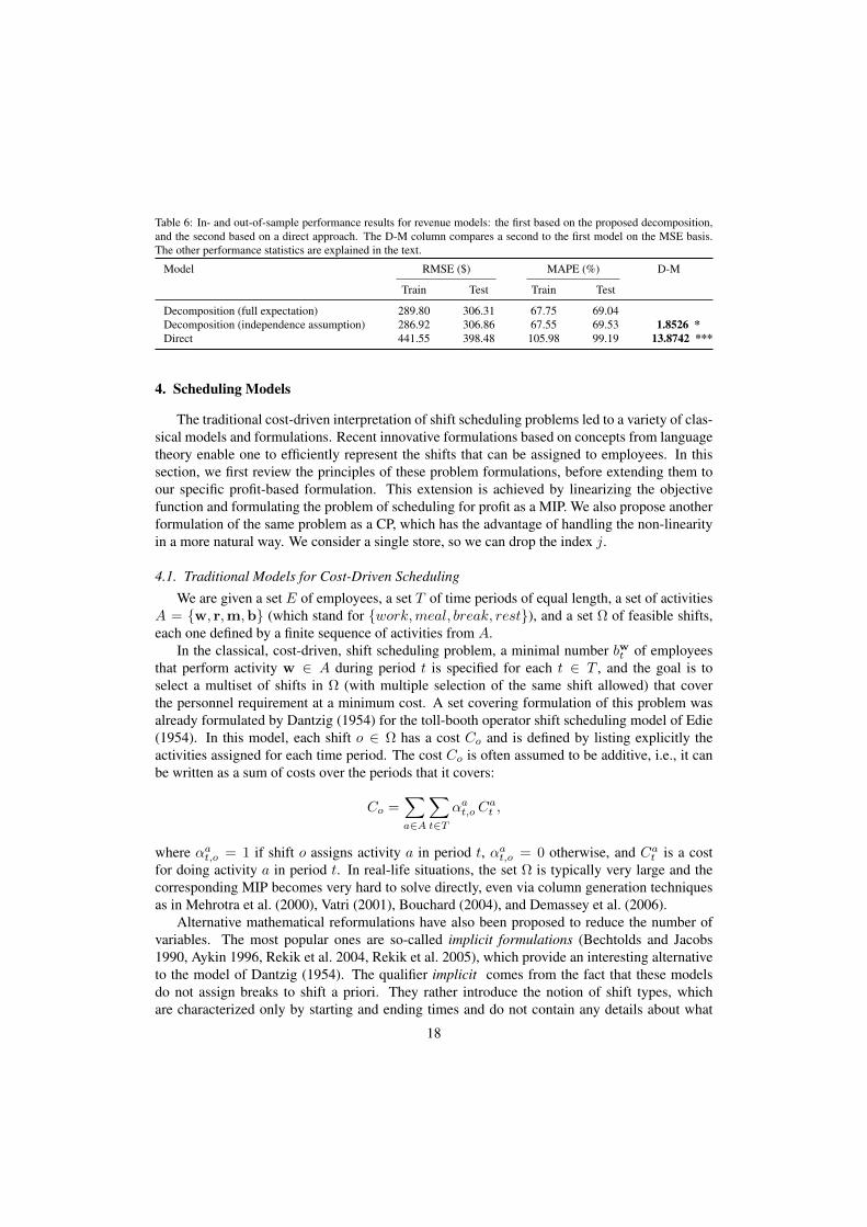
Table 6: In- and out-of-sample performance results for revenue models: the first based on the proposed decomposition,and the second based on a direct approach. The D-M column compares a second to the first model on the MSE basis.The other performance statistics are explained in the text.

Model RMSE ($) MAPE (%) D-M

Train Test Train Test

Decomposition (full expectation) 289.80 306.31 67.75 69.04Decomposition (independence assumption) 286.92 306.86 67.55 69.53 1.8526 *Direct 441.55 398.48 105.98 99.19 13.8742 ***

4. Scheduling Models

The traditional cost-driven interpretation of shift scheduling problems led to a variety of clas-sical models and formulations. Recent innovative formulations based on concepts from languagetheory enable one to efficiently represent the shifts that can be assigned to employees. In thissection, we first review the principles of these problem formulations, before extending them toour specific profit-based formulation. This extension is achieved by linearizing the objectivefunction and formulating the problem of scheduling for profit as a MIP. We also propose anotherformulation of the same problem as a CP, which has the advantage of handling the non-linearityin a more natural way. We consider a single store, so we can drop the index j.

4.1. Traditional Models for Cost-Driven Scheduling

We are given a set E of employees, a set T of time periods of equal length, a set of activitiesA = w, r,m,b (which stand for work,meal, break, rest), and a set Ω of feasible shifts,each one defined by a finite sequence of activities from A.

In the classical, cost-driven, shift scheduling problem, a minimal number bwt of employeesthat perform activity w ∈ A during period t is specified for each t ∈ T , and the goal is toselect a multiset of shifts in Ω (with multiple selection of the same shift allowed) that coverthe personnel requirement at a minimum cost. A set covering formulation of this problem wasalready formulated by Dantzig (1954) for the toll-booth operator shift scheduling model of Edie(1954). In this model, each shift o ∈ Ω has a cost Co and is defined by listing explicitly theactivities assigned for each time period. The cost Co is often assumed to be additive, i.e., it canbe written as a sum of costs over the periods that it covers:

Co =∑a∈A

∑t∈T

αat,o Cat ,

where αat,o = 1 if shift o assigns activity a in period t, αat,o = 0 otherwise, and Cat is a costfor doing activity a in period t. In real-life situations, the set Ω is typically very large and thecorresponding MIP becomes very hard to solve directly, even via column generation techniquesas in Mehrotra et al. (2000), Vatri (2001), Bouchard (2004), and Demassey et al. (2006).

Alternative mathematical reformulations have also been proposed to reduce the number ofvariables. The most popular ones are so-called implicit formulations (Bechtolds and Jacobs1990, Aykin 1996, Rekik et al. 2004, Rekik et al. 2005), which provide an interesting alternativeto the model of Dantzig (1954). The qualifier implicit comes from the fact that these modelsdo not assign breaks to shift a priori. They rather introduce the notion of shift types, whichare characterized only by starting and ending times and do not contain any details about what

18

0

1

r

r

2w

ww

3b

4w

w

5m

w

6w

r

7r

r

Figure 6: A DFA Π with each state represented as a circle, the two final states are shaded, and each transition as an arc.

happens in between. Typically, these models capture the number of employees assigned to eachshift type and to each break with different sets of variables. From an optimal solution to such animplicit model, one can retrieve the number of employees assigned to each shift type and eachbreak, and construct an optimal set of shifts through a polynomial-time procedure.

More recently, Côté et al. (2011a,b) showed how to exploit the expressiveness of automataand context-free grammars to formulate MIP models in which any feasible shift is representedby a word in a regular language, and the set of admissible staffing solutions (which correspondto an admissible collection of shifts) is defined implicitly by an integral polyhedron that can beconstructed automatically even for complex work regulations such as those mentioned earlier. Inwhat follows, we will adapt this approach to our profit-maximizing problem. Our use of automatatogether with CP for this type of scheduling problem is novel.

4.2. Regular Language and Workforce Scheduling

Following Côté et al. (2011a,b), we will represent each admissible shift by a word definedover the alphabet A = w, r,m,b, where the ith letter in the word indicates the activity ofthe employee during the ith time period of its shift. In our case study, those time periods have15 minutes. As an illustration, the word “wwbwwwmmwwww” symbolizes a 3-hour shiftwhere the employee works for 30 minutes, takes a 15 minutes break, gets back to work for 45minutes, takes a lunch break of 30 minutes, and goes back to work for the remaining hour.

To recognize the valid words, i.e., those that correspond to admissible shifts, we define adeterministic finite automaton (DFA) that specifies the rules that regulate the transitions in thesequence of activities that can be assigned to an employee in a shift. The DFA is defined as a5-tuple Π = 〈Q,A, τ, q0, F 〉, where

• Q is the finite set of states;

• A is the alphabet;

• τ : Q×A→ Q is the transition function;

• q0 ∈ Q is the initial state;

• and F ⊆ Q is a set of final states.

A word is recognized by a DFA if, by processing its symbols one by one from the initial stateand following the transitions, we end up in a final state after processing the last symbol.

Figure 6 illustrates a DFA Π that recognizes a language defined over the alphabet A. It hasQ = 0, 1, . . . , 6, q0 = 0 and F = 5, 6. This language contains, for instance, the words“wwbwwmww”, “rr” and “r”, but it does not include the words “wwr” or “wwbm” as theyare not recognized by Π.

19

0.0

1.1

r

1.2r

2.1

w

2.2

w

w 2.3

w

w

3.2

b

3.3

b

3.4

b

4.3

w

4.4

w

w 4.5

w

w

5.4

m

5.5

m

w 5.6

m

w

6.5

w

6.6

w

r 6.7

w

r

7.1

r

7.2r 7.3r 7.4r 7.5r 7.6r 7.7r

Figure 7: An automaton Π7 that recognizes all the words of length ` = 7 of the language defined by Π

From a given DFA that specifies the set of admissible shifts, one can obtain a MIP by re-formulating the constraints expressed in the DFA as a set of network flow constraints which,together with the profit-maximizing objective, define a network flow optimization problem. Thisis similar to what was done by Côté et al. (2011a). For this, we first introduce for each word(each admissible shift) of length ` the binary decision variables xat = 1 if the word has activitya ∈ A in position (time period) t, xat = 0 otherwise, for t = 1, . . . , `. This representationpermits one to directly formulate complex rules that regulate the sequence of activities (e.g., anemployee must work at least an hour before taking a break), which are usually complex to han-dle by traditional approaches, in a much more efficient way by expressing them as network flowconstraints.

To control the length of words that can be accepted by the DFA, we derive from Π anotherautomaton Π` that recognizes only the sequences of length ` that are accepted by Π (Pesant,2004). The automaton Π` is represented by an acyclic directed layered graph with ` + 1 layers,whose set of states in layer t has the form q.t : q ∈ N t, where N t ⊆ Q, for t = 0, . . . , `.One has N0 = q0 and N ` ⊆ F . Figure 7 illustrates the automaton Π7 that represents all thewords of length ` = 7 included in the language defined by the automaton Π of Figure 6. Eachword is obtained by taking a path from node 0.0 to one of the two shaded nodes, and collectingthe symbols on the arcs taken along the road. The lower branch corresponds to an off day (nowork). The automaton Π`, with ` equal to the number of periods in the day, can be used toconstruct a graph G as in Figure 7, from which the network flow formulation is obtained. Fort = 0, . . . , ` and each q ∈ N t, each pair q.t is a node of G and each transition in Π` is an arcofG. A flow variable stq,a,q′ is assigned to each arc ofG, indicating that the symbol a is assignedto position t in the sequence by transiting from state q to state q′ of Π (and state q.(t− 1) to stateq′.t) of Π`). The unique element q0 of N0 is identified as the source node, and the nodes q.`in N ` correspond to the set of final states F of Π. Note that the actual length of the shift can beless than `; this can be handled by assigning the activity r to some of the periods, usually at the

20

beginning or at the end of the shift.Let

πaq,q′ =

1, if the transition function τ allows a transition from state q ∈ Q

to state q′ ∈ Q with label a ∈ A in the automaton Π,

0, otherwise.

A word of length ` is included in the language defined by Π if and only if its corresponding flowvariables satisfy the following constraints:∑

a∈A

∑q∈Q

s1q0,a,q = 1 (6)

∑a∈A

∑q′∈Q

st−1q′,a,q =

∑a∈A

∑q′∈Q

stq,a,q′ ∀t ∈ 2, ..., `, q ∈ Q (7)

∑a∈A

∑q∈Q

∑f∈F

s`q,a,f = 1 (8)

stq,a,q′ ≤ πaq,q′ ∀t ∈ 1, ..., `, a ∈ A, (q, q′) ∈ Q2 (9)∑(q,q′)∈Q2

stq,a,q′ = xat ∀t ∈ 1, ..., `, a ∈ A (10)

stq,a,q′ ∈ 0, 1 ∀t ∈ 1, ..., `, a ∈ A, (q, q′) ∈ Q2. (11)

Constraints (6)–(8) ensure that one unit of flow enters the graph by the source and leaves it bya final state, and that the amount of flow entering and leaving each other node in the graph isthe same. Constraints (9) guarantee that the transition function τ of Π is respected, whereasconstraints (10) link the decision variables xat and the flow variables. Finally, constraints (11)define the domain of the flow variables.

4.3. Mixed Integer Programming for Schedule Construction

We are now ready to formulate our profit-driven workforce scheduling problem as a MIPby building over the network flow formulation of constraints on feasible shifts as given in theprevious subsection. We consider a single store j at a time, so we drop the index j. We use E todenote the set of employees, D for the set of days for which we want to construct the schedule(e.g., Monday to Sunday if it is over a week, or a single element if it is over a single day), and Tdfor the set of time periods when the store is open on day d. LetM = 0, 1, . . . , |E| (the possiblenumber of employees that can perform a given task during a given period) and A = w,b,m(the non-rest activities, which are the only ones considered to determine the real length of a shift).We introduce two sets of binary variables: xe,ad,t indicates if employee e performs task a duringperiod t on day d, while ym,ad,t indicates if exactly m employees perform task a during period ton the day d. Each flow variable se,d,tq,a,q′ indicates whether employee e is transiting from state q

21

to state q′ (of Π) during period t of day d by performing task a. Our MIP formulation is:

max∑m∈M

∑d∈D

∑t∈Td

(rd,t(m) ym,wd,t −

∑a∈A

m Cad,t ym,ad,t

)(12)

subject to ∑a∈A

∑q∈Q

se,d,1q0,a,q = 1 ∀e ∈ E, d ∈ D (13)

∑a∈A

∑q′∈Q

se,d,t−1q′,a,q =

∑a∈A

∑q′∈Q

se,d,tq,a,q′ ∀e ∈ E, d ∈ D, t ∈ 2, ..., |Td|, q ∈ Q

(14)∑a∈A

∑q∈Q

∑f∈F

se,d,|Td|q,a,f = 1 ∀e ∈ E, d ∈ D (15)

se,d,tq,a,q′ ≤ πaq,q′ ∀e ∈ E, d ∈ D, t ∈ Td, a ∈ A, (q, q′) ∈ Q2

(16)∑(q,q′)∈Q2

se,d,tq,a,q′ = xe,ad,t ∀e ∈ E, d ∈ D, t ∈ Td, a ∈ A

(17)∑e∈E

xe,ad,t =∑m∈M

mym,ad,t ∀d ∈ D, t ∈ Td, a ∈ A (18)∑a∈A

xe,ad,t = 1 ∀e ∈ E, d ∈ D, t ∈ Td (19)∑m∈M

ym,ad,t = 1 ∀d ∈ D, t ∈ Td, a ∈ A (20)

δ−e ≤∑t∈Td

∑a∈A

xe,ad,t ≤ δ+e ∀e ∈ E, d ∈ D (21)

∆−e ≤∑d∈D

∑t∈Td

∑a∈A

xe,ad,t ≤ ∆+e ∀e ∈ E (22)

se,d,tq,a,q′ ∈ 0, 1 ∀e ∈ E, d ∈ D, t ∈ Td, a ∈ A, (q, q′) ∈ Q2

(23)

xe,ad,t ∈ 0, 1 ∀e ∈ E, d ∈ D, t ∈ Td, a ∈ A(24)

ym,ad,t ∈ 0, 1 ∀m ∈M, d ∈ D, t ∈ Td, a ∈ A(25)

In the objective function, we find the sales curves rd,t(·) defined in (1) (where we have droppedthe store index j), which give the expected revenue from sales in each time period as a function ofthe number of working employees, and the total salary expenses, where Cad,t is the per-employeecost for performing activity a during period t on day d. We want to maximize the total expectedprofit. We have used binary variables ym,ad,t ∈ 0, 1 instead of integer variables yad,t ∈ Mto represent the number of employees performing each activity in each time period becauseit provides a linear MIP formulation of the problem, despite the nonlinear sales curves in the

22

Figure 8: A sales curve defined over 1, . . . , 8 and its PLA with p = 4 pieces separated at 2, 4, and 6.

objective function. Constraints (13)–(17) guarantee that all shifts assigned to employees onday d correspond to words of length |Td| in the language defined by Π, by deriving a flowproblem over the variables se,d,tq′,a,q and linking them to the variables xe,ad,t (as in subsection 4.2).Constraints (18) link the variables xe,ad,t and ym,ad,t , whereas constraints (19) guarantee that a singletask a is assigned to each employee e for every period t of a day d, and constraints (20) ensure thatym,ad,t captures the number of employees performing task a in period t of day d. Constraints (21)–(22) impose a minimum duration of δ−e and a maximum duration of δ+

e to the shift length of eachemployee (excluding the r activity) over any given day d, as well as a minimum duration of ∆−eand maximum duration of ∆+

e for the total shift duration over all days covered by the schedule(e.g., over the week). Finally, constraints (23)–(25) define the domain of all variables.

4.4. Estimation of the Revenues by Piecewise Linear Approximations (PLA)The linearization of the objective function in our MIP formulation has introduced a huge

number of binary variables ym,ad,t , which increases significantly the size of the problem. Oneway to reduce this size is to approximate the sales curves by piecewise linear functions. Ifp ≥ 1 denotes the number of linear pieces in the approximation, the PLA formulation, whichwe denote by MIP-PLAp, use p binary variables to indicate the piece in which we are, and aninteger variable yad,t ≥ 0 to indicate the number of employees performing activity a in period tof day d. Typically, the sales curves are concave, in which case the PLA will underestimate theexpected revenue (see Figure 8). When p = |E| − 1, MIP-PLAp is equivalent to the originalMIP formulation, whereas if p < |E| − 1, MIP-PLAp is an estimation of the MIP, so the optimalsolution of MIP-PLAp might not be optimal for MIP. However, any feasible solution to MIP-PLAp is feasible for MIP, because the PLA does not modify the constraints.

4.5. Constraint Programming for Schedule ConstructionWe now consider another efficient approach, based on a problem formulation as a CP. This

formulation handles the non-linearity naturally without altering the model by using approxima-23

tions and without adding extra variables. Our CP formulation is based on three sets of variables:xed,t specifies the activity a ∈ A performed by employee e in period t of day d, yad,t represents thenumber of employees that perform activity a in period t of day d, and sed,t ∈ Q describes the stateof the automaton that led to the assignment of the activity performed by employee e in period tof day d. We represent a transition from state q to state q′ labeled by a by the triplet 〈q, a, q′〉,and we define Θ as the set of triplets 〈q, a, q′〉 that correspond to transitions allowed under theDFA Π. Before stating the CP model, we recall to the reader that in Constraint Programmingthe expression “(variable = value)”, when used within a constraint, is automatically transformed(known as reification) into a boolean variable that takes value 1 when the expression holds and 0otherwise. The proposed CP model is then:

max∑d∈D

∑t∈Td

(rd,t(y

wd,t)−

∑a∈A

Cad,t yad,t

)(26)

subject tosed,0 = q0 ∀e ∈ E, d ∈ D (27)

〈sed,t−1, xed,t, s

ed,t〉 ∈ Θ ∀e ∈ E, d ∈ D, t ∈ 1, ..., |Td|

(28)

sed,|Td| ∈ F ∀e ∈ E, d ∈ D (29)∑e∈E

(xed,t = a) = yad,t ∀d ∈ D, t ∈ Td, a ∈ A (30)

δ−e ≤∑t∈Td

(xed,t 6= r) ≤ δ+e ∀e ∈ E, d ∈ D (31)

∆−e ≤∑d∈D

∑t∈Td

(xed,t 6= r) ≤ ∆+e ∀e ∈ E (32)

sed,t ∈ Q ∀e ∈ E, d ∈ D, t ∈ Td (33)

xed,t ∈ A ∀e ∈ E, d ∈ D, t ∈ Td (34)

yad,t ∈M ∀a ∈ A, d ∈ D, t ∈ Td (35)

The objective function in (26) is the same as in the MIP, but is expressed more concisely, as itcan use directly the integer variables ywd,t. The constraints (27)–(29) ensure that the shift per-formed by any employee e over a day d is recognized as a word of length |Td| in the languagedefined by Π. Constraints (27) and (29) ensure that the exploration of the automaton begins at itsinitial state and ends in a final state (in F ), whereas constraints (28) guarantee that the transitionfunction τ of the DFA is respected when moving from state to state. Constraints (30) link thexed,t and yad,t variables. Constraints (31)–(32) guarantee that the length of each employee’s shiftrespects the minimum and maximum durations defined over a day and over a week, respectively.Finally, constraints (33)–(35) define the domain of all variables. In constraint programming ter-minology, contraints (28) are known as table constraints and contraints (30) as global cardinalityconstraints. Most constraint programming solvers can handle these families of constraints usingspecial-purpose algorithms. This CP is exactly equivalent to the MIP introduced earlier. How-ever, the two formulations give rise to different solutions methods, whose performance can bevery different. In particular, the large number of binary variables in the MIP can have a significantimpact on the speed of resolution.

24

5. Solving the Scheduling Problem for the Case Study: Numerical Comparisons

We have implemented the MIP and CP formulations of Section 4 for our case study, andsolved them using the ILOG CPLEX optimization tool on 2.1 GHz dual core processors with3.5 GB of memory. In this section, we demonstrate and compare the accuracy and the efficiencyof the proposed approaches to construct schedules for one day and one week, while consideringthe work regulation rules of the retailer. Note that a new labor regulation impacting schedulingwas put in place by the retailer in all its stores after the period for which we have data. Althoughthe regulations defined over a day did not change, the new regulations impose a new set of rulescommon to all stores, over a week. Before the change, each store manager was constructingweekly schedules according to his own set of rules, which could potentially change betweenweeks. In this sense, we do not have full access to the exact weekly scheduling rules for theperiod studied, and therefore a fair comparison between our schedules and the schedules histori-cally used in the stores can only be perform over a day. However, our models integrate the newregulation of the retailer and the performance of the schedules they provide for each week canstill be measured from the gap between the expected profit they generate and an accurate upperbound of the maximum expected profit that can be generated over a week while respecting theregulations.

5.1. Work regulation rules and other informationIn addition to the generic constraints given in our MIP or CP formulation, there are other

daily and weekly constraints specific to our retailer. In their formulation, two types of employeesare distinguished: part-time and full-time.

• Daily regulations:

– Work and rest distribution: each day, the employee can have a day off or work forone shift;

– Shift duration: a shift over a day lasts from 3 to 8 hours;

– Break and meal distribution: non-working stretches (break, meal, rest) have to beseparated by at least one hour of work;

– Break and meal authorization: an employee working a shift lasting less than 5 hoursmust take a single 15-minute break, whereas an employee working a shift of 5 hoursor more must take two 15-minute breaks, separated by a 30-minute meal break.

– Minimum presence:

* Stores with external back stores must have a minimum of two employees at alltimes during opening hours, else a minimum of one employee is required;

* Part-time employees must never work alone, a full-time employee must alwaysbe present..

• Weekly regulations:

– Work and rest distribution

* An employee cannot work more than 5 shifts in a week;

* An employee must have two consecutive days off in a week or one week-endday off;

25

0

1

2

3

4

5

6

7

8

9

10

11

12

13

14

15

16

17

18

19

20

21

22

r

w

w

w

w

w

b

w

w

w

w

w

m

m

m

m

w

w

w

w

w

b

w

w

w

w

w

rw

Figure 9: Illustration of the DFA Π that defines the formal language used by our model.

– Shift duration

* A part-time employee must work between 10 hours and 30 hours over a week;

* A full-time employee must work between 25 hours and 40 hours over a week.

We used data coming from 15 stores, for 5089 days in total (the same portion of data thatwas used to evaluate the forecasting models). In every store, half the workforce are full-timeemployees, and we must have at least three employees with a full-time contract. These storeshire between 4 and 9 employees, and their opening hours vary from 9 hours to 12 hours per day.Table 7 gives additional details on these values. Only stores 14 and 15 have an external backstore. Each day is split into 15-minute intervals. All employees earn the same hourly salary,from which the costs Cat are extracted. Breaks and meals are not paid. Note that, although thenumber of employees of each kind (partial time vs full time) is fixed, the amount of time spentworking on the floor over a day and a week by each of them is only constrained to be inside aspecific range, namely [δ−e , δ

+e ] for a day and [∆−e ,∆

+e ] for a week for every employee e ∈ E,

so the total cost of employees over a day or a week has to be determined during the optimizationprocess.

5.2. Automaton for retail store scheduling

Figure 9 illustrates the automaton Π that defines the formal language for our model. Thisautomaton is used to construct a word for each employee, that represents his admissible dailyshift, in which the sequence of activities he performs obeys all the sequencing rules (e.g., anemployee must work at least one hour before his first break, he must work for a shift of at leastfive hours to be allowed to take two breaks, etc.). The other regulation rules are incorporatedusing traditional MIP and CP constraints based on the number of occurrences of each activity inthe word of each employee or the states of the automaton explored by an employee.

To formulate these extra constraints, we use E to denote the set of full-time employees, Dfor the set of the first four days of the week (Monday to Thursday), D for the set of weekenddays (Saturday and Sunday), and q1 to denote state 1 of the automaton of Figure 9. For the extraconstraints in the MIP formulation, we introduce two new sets of binary variables: ved indicates

26

if employee e is off for both day d and the following day, while ze indicates if employee e has aday off over the weekend. The extra constraints for the MIP are:

δ−e∑tinTd

se,d,tq0,w,q1 ≤∑t∈Td

∑a∈A

xe,ad,t ≤ δ+e

∑tinTd

se,d,tq0,w,q1 ∀e ∈ E, d ∈ D (36)

∑t∈Td

y0,wd,t = 0 ∀d ∈ D (37)

∑e∈E

xe,rd,t ≤ |E| − 1 ∀d ∈ D, t ∈ Td (38)

∑d∈D

se,d,|Td|q0,r,q0 ≥ 2 ∀e ∈ E, d ∈ D (39)

2 ved ≤ se,d,|Td|q0,r,q0 + s

e,d+1,|Td+1|q0,r,q0 ∀e ∈ E, d ∈ D (40)

ze ≤∑d∈D

se,d,|Td|q0,r,q0 ∀e ∈ E (41)

ze +∑d∈D

ved ≥ 1 ∀e ∈ E (42)

ved ∈ 0, 1 ∀e ∈ E, d ∈ D (43)ze ∈ 0, 1 ∀e ∈ E (44)

while the extra constraints to be added to the CP are:

δ−e∑t∈Td

(sed,t = q1

)≤∑t∈Td

(xed,t 6= r

)≤ δ+

e

∑t∈Td

(sed,t = q1

)∀e ∈ E, d ∈ D

(45)

ywd,t ≥ 1 ∀d ∈ D, t ∈ Td(46)∑

e∈E

(xed,t 6= r

)≥ 1 ∀d ∈ D, t ∈ Td

(47)∑d∈D

(sed,|Td| = q0

)≥ 2 ∀e ∈ E, d ∈ D

(48)(∑d∈D

((∑t∈Td

(xed,t = w) = 0

)∧ (

∑t∈Td+1

(xed+1,t = w) = 0

))≥ 1)

∨(∑d∈D

(∑t∈Td

(xed,t = w) = 0

)≥ 1)

∀e ∈ E.

(49)

The constraints (36) and (45) are reformulation of the generic constraints (21) and (31) that stillguarantee that the length of each employee’s shift respects the minimum and maximum durationsdefined over a day, while adding the possibility that an employee does not work over a day (i.e.,the employee has a day off). The constraints (37) and (46) ensure that there is at least one

27

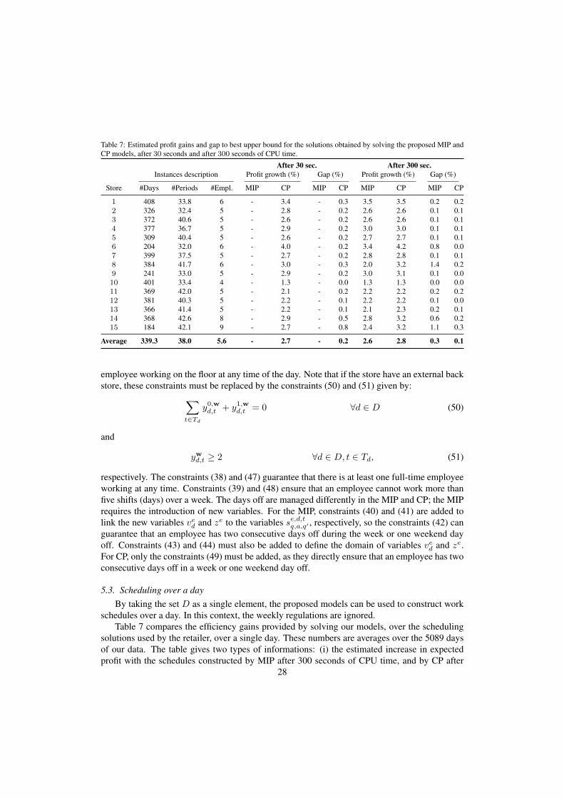
Table 7: Estimated profit gains and gap to best upper bound for the solutions obtained by solving the proposed MIP andCP models, after 30 seconds and after 300 seconds of CPU time.

After 30 sec. After 300 sec.Instances description Profit growth (%) Gap (%) Profit growth (%) Gap (%)

Store #Days #Periods #Empl. MIP CP MIP CP MIP CP MIP CP

1 408 33.8 6 - 3.4 - 0.3 3.5 3.5 0.2 0.22 326 32.4 5 - 2.8 - 0.2 2.6 2.6 0.1 0.13 372 40.6 5 - 2.6 - 0.2 2.6 2.6 0.1 0.14 377 36.7 5 - 2.9 - 0.2 3.0 3.0 0.1 0.15 309 40.4 5 - 2.6 - 0.2 2.7 2.7 0.1 0.16 204 32.0 6 - 4.0 - 0.2 3.4 4.2 0.8 0.07 399 37.5 5 - 2.7 - 0.2 2.8 2.8 0.1 0.18 384 41.7 6 - 3.0 - 0.3 2.0 3.2 1.4 0.29 241 33.0 5 - 2.9 - 0.2 3.0 3.1 0.1 0.010 401 33.4 4 - 1.3 - 0.0 1.3 1.3 0.0 0.011 369 42.0 5 - 2.1 - 0.2 2.2 2.2 0.2 0.212 381 40.3 5 - 2.2 - 0.1 2.2 2.2 0.1 0.013 366 41.4 5 - 2.2 - 0.1 2.1 2.3 0.2 0.114 368 42.6 8 - 2.9 - 0.5 2.8 3.2 0.6 0.215 184 42.1 9 - 2.7 - 0.8 2.4 3.2 1.1 0.3

Average 339.3 38.0 5.6 - 2.7 - 0.2 2.6 2.8 0.3 0.1

employee working on the floor at any time of the day. Note that if the store have an external backstore, these constraints must be replaced by the constraints (50) and (51) given by:∑

t∈Td

y0,wd,t + y1,w

d,t = 0 ∀d ∈ D (50)

and

ywd,t ≥ 2 ∀d ∈ D, t ∈ Td, (51)

respectively. The constraints (38) and (47) guarantee that there is at least one full-time employeeworking at any time. Constraints (39) and (48) ensure that an employee cannot work more thanfive shifts (days) over a week. The days off are managed differently in the MIP and CP; the MIPrequires the introduction of new variables. For the MIP, constraints (40) and (41) are added tolink the new variables ved and ze to the variables se,d,tq,a,q′ , respectively, so the constraints (42) canguarantee that an employee has two consecutive days off during the week or one weekend dayoff. Constraints (43) and (44) must also be added to define the domain of variables ved and ze.For CP, only the constraints (49) must be added, as they directly ensure that an employee has twoconsecutive days off in a week or one weekend day off.

5.3. Scheduling over a dayBy taking the set D as a single element, the proposed models can be used to construct work

schedules over a day. In this context, the weekly regulations are ignored.Table 7 compares the efficiency gains provided by solving our models, over the scheduling

solutions used by the retailer, over a single day. These numbers are averages over the 5089 daysof our data. The table gives two types of informations: (i) the estimated increase in expectedprofit with the schedules constructed by MIP after 300 seconds of CPU time, and by CP after

28

Table 8: Evolution of the gap of the solutions identified by CP when building schedules over a week with two hours ofCPU time, according to the best upper bound obtained after 24 hours.

Instances description Gap with upper bound obtained from MIP (in %)

Store #Weeks #Periods #Empl. after 30 min after 60 min after 120 min

1 37 236 6 2.2 2.0 1.62 23 224 5 1.9 1.7 1.53 21 282 5 3.8 3.6 3.44 34 256 5 2.5 2.3 2.15 17 280 5 4.4 4.0 3.66 15 232 6 2.8 2.5 2.47 38 262 5 3.1 2.7 2.58 38 288 6 3.4 3.3 3.19 14 230 5 2.0 1.8 1.610 36 234 4 2.0 1.9 1.711 22 294 5 3.4 3.3 3.212 23 282 5 2.9 2.7 2.613 22 288 5 3.0 2.8 2.714 18 296 8 1.9 1.7 1.715 12 292 9 8.3 7.2 6.9

Average 24.7 265.1 5.6 3.2 2.9 2.7

30 seconds and 300 seconds of CPU time, compared with the schedules used by the retailer; and(ii) the gap between those MIP and CP solutions and the best upper bound extracted from the MIPsolution after 300 seconds. As the solutions provided by solving MIP with PLA generate lessprofit than the solutions of the full MIP while using the same amount of CPU time to constructfeasible schedules, we always used the full MIP (no PLA) in this section. For many instances,the MIP failed to return a feasible solution after 30 seconds; for this reason we do not reportthe results. The solutions returned by either MIP or CP after 300 seconds are very accurate.They are nearly optimal with a respective average gap of only 0.3% and 0.1%, and correspondto estimated profit increases of 2.6% and 2.8%, respectively (in terms of the estimated expectedsales given by the sales curves). CP seems to provide a slightly larger profit growth than MIP,and also provides good solutions already after 30 seconds. Unfortunately, CP does not providean upper bound on the optimal value during the resolution. In practice, the CP approach seemsto be the most efficient method overall.

5.4. Scheduling over a week

Only CP was able to construct feasible weekly schedules consistently in less than two hoursof CPU time, for the week instances in our data. For MIP, even the combination with PLAwith a single linear piece (MIP-PLA1) failed to provide feasible solutions for over 30% of theweeks. Table 8 shows the evolution of the gap between the solutions identified by solving theCP model after 30 minutes, 60 minutes, and 120 minutes of CPU time, and the best upper boundextracted after 24 hours of CPU time with the MIP model. Given that the weekly schedulesused historically in the stores do not satisfy the new rules imposed by the retailer, we cannotmake a fair comparison with our solutions. This is why we only compare with an upper bound.The quality of the schedules constructed by CP is demonstrated by the small average gap (lessthan 3% after 60 minutes) between the value of these solutions the corresponding upper bounds(which are likely to be larger than the optimal values).

29

6. Conclusion

We have proposed a new methodology to construct schedules for the non-identical workforceof retail stores, to optimize the expected net revenue, based on sales curves that provide theexpected revenue from sales as a function of the number of working employees on the floor. Wedeveloped two formulations of the profit-maximization problem, as a MIP and as a CP, whichincorporate both the operating revenue and the context of a non-identical workforce, and consideremployees as a source a revenue, an approach that differs markedly from the traditional approachwhere employees are considered as a sole expense and have the same specificity (availability,skills, etc.).

Our numerical experiments indicate that although both CP and MIP are able to provide near-optimal solutions in a few minutes for the scheduling problems over one day, CP is faster andprovides better solutions. When constructing schedules for larger problem instances (over aweek), CP provides a solution that respect all the regulation rules of the retailer in less than anhour of CPU time, with a gap of around 3% with respect to the upper bound given by the solutionof the linear relaxation of the equivalent MIP model obtained after 24 hours of computation. Forthe MIP, we were unable to consistently generate feasible solution within an hour.

Further work will focus on the elaboration of better branching and cutting strategies to helpthe resolution of CP, as well as the consideration of multiple skills and multiple working ac-tivities. We also plan to improve the accuracy of the staffing forecast models by consideringinter-period dependence and events, such as customers that leave the store before buying itemsin order to come back later the same day, when more sellers are available.

References

Avramidis, A.N., Chan, W., Gendreau, M., L’Ecuyer, P., Pisacane, O., 2010. Optimizing daily agent scheduling in amultiskill call centers. European Journal of Operational Research 200, 822–832.

Aykin, T., 1996. Optimal shift scheduling with multiple break windows. Management Science 42, 591–602.Bechtolds, S., Jacobs, L., 1990. Implicit optimal modeling of flexible break assigments. Management Science 36,

1339–1351.Bouchard, M., 2004. Optimisation des pauses dans le problème de fabrication des horaires avec quarts de travail.

Memoire de maitrise, Ecole Polytechnique de Montreal.Brockwell, P.J., Davis, R.A., 1991. Time Series: Theory and Methods. 2nd ed., Springer.Chapados, N., Joliveau, M., Rousseau, L.M., 2011. Retail store workforce scheduling by expected operating income

maximization, in: Achterberg, T., Beck, J. (Eds.), Integration of AI and OR Techniques in Constraint Programmingfor Combinatorial Optimization Problems. Springer Berlin / Heidelberg. volume 6697 of Lecture Notes in ComputerScience, pp. 53–58.

Côté, M.C., Gendron, B., Quimper, C.G., Rousseau, L.M., 2011a. Formal languages for integer programming modelingof shift scheduling problem. Constraints 16, 54–76.

Côté, M.C., Gendron, B., Rousseau, L.M., 2011b. Grammar-based integer programming models for multi-activity shiftscheduling. Management Science 57, 151–163.

Dantzig, G., 1954. A comment on Edie’s traffic delay at toll booths. Journal of Operation Research Society of America2, 339–341.

Demassey, S., Pesant, G., Rousseau, L.M., 2006. A cost-regular based hybrid column generation approach. Constraints11, 315–333.

Diebold, F.X., Mariano, R.S., 1995. Comparing predictive accuracy. Journal of Business & Economic Statistics 13,253–263.

Edie, L., 1954. Traffic delays at toll booths. Operations Research 2, 107–138.Hilbe, J.M., 2011. Negative Binomial Regression. Second edition ed., Cambridge University Press, Cambridge, UK.Hyndman, R.J., Razbash, S., Schmidt, D., 2012. forecast: Forecasting functions for time series and linear models. URL:

http://CRAN.R-project.org/package=forecast. r package version 3.21.Kabak, Ö., Ülengin, F., Aktas, E., Önsel, S., Topcu, Y.I., 2008. Efficient shift scheduling in the retail sector through

two-stage optimization. European Journal of Operational Research 184, 76–90.30

Koole, G., Pot, A., 2011. A note on profit maximization and monotonicity for inbound call centers. Operations Research59, 1304–1308.

Lam, S.Y., Vandenbosch, M., Hulland, J., Pearce, M., 2001. Evaluating promotions in shopping environments: Decom-posing sales response into attraction, conversion, and spending effects. Marketing Science 20, 194–215.

Lam, S.Y., Vandenbosch, M., Pearce, M., 1998. Retail sales force scheduling based on store traffic forecasting. Journalof Retailing 74, 61–88.

Lehmann, E.L., Casella, G., 1998. Theory of Point Estimation. Second ed., Springer.Makridakis, S.G., Wheelwright, S.C., Hyndman, R.J., 1997. Forecasting: Methods and Applications. 3rd ed., Wiley.Mani, V., Kesavan, S., Swaminathan, J.M., 2011. Understaffing in retail stores. Working Paper.McCullagh, P., 1980. Regression models for ordinal data (with discussion). Journal of the Royal Statistical Society B

42, 109–142.McCullagh, P., Nelder, J.A., 1989. Generalized Linear Models. Second ed., Chapman & Hall, London.McCulloch, C.E., Searle, S.R., Neuhaus, J.M., 2008. Generalized, Linear, and Mixed Models. Wiley Series in Probability

and Statistics. second ed., John Wiley & Sons, Hoboken, NJ.Mehrotra, A., Murthy, K., Trick, M., 2000. Optimal shift scheduling: A branch-and-price approach. Naval Research

Logistics 47, 185–200.Netessine, S., Fisher, M.L., Krishnan, J., 2010. Labor planning, execution, and retail store performance: an exploratory

investigation. Working Paper, University of Pennsylvania.Perdikaki, O., Kesavan, S., Swaminathan, J.M., 2012. Effect of traffic on sales and conversion rates of retail stores.

Manufacturing and Service Operations Management 14, 145–162.Pesant, G., 2004. A regular language membership constraint for finite sequences of variables., in: Proceedings of the

tenth international conference on principles and practice of Constraint Programming (CP 2004), pp. 482–495.Pinheiro, J.C., Bates, D.M., 2000. Mixed Effects Models in S and S-Plus. Springer-Verlag, New York, NY.Rekik, M., Cordeau, J.F., Soumis, F., 2004. Using Benders decomposition to implicitly model tour scheduling. Annals

of Operations Research 128, 111–133.Rekik, M., Cordeau, J.F., Soumis, F., 2005. Implicit shift scheduling with multiple breaks ans work stretch duration

restrictions. Publication GERAD-2005-15 .Thompson, G.M., 1995. Labor scheduling using npv estimates of the marginal benefit of additional labor capacity.

Journal of Operations Management 13, 67–86.Ton, Z., 2009. The effect of labor on profitability: The role of quality. Working Paper, Harvard Business School.U.S. Census Bureau (Ed.), 2011. Statistical Abstract of the United States: 2012. U.S. Census Bureau. chapter Wholesale

and Retail Trade.Vatri, E., 2001. Integration de la generation de quart de travail et de l’attribution d’activites. Memoire de maitrise, Ecole

Polytechnique de Montreal.

31