Rethinking the choice between core and headline in�ation:

Does it matter which one to target?

Chi-Young Choi

University of Texas at Arlington

Jianning Kong�

Shandong University

Donggyu Sul

University of Texas at Dallas

December 3, 2016

Abstract

This study addresses two important questions relating to the appropriate measure of in�ation

for monetary policy purposes: (1) whether core in�ation is statistically di¤erent from headline

in�ation in estimating underlying in�ation; and (2) whether core in�ation is a better predictor

of future headline in�ation. Our answer to both questions is �No�. We �nd that headline

in�ation is not statistically di¤erent from popular alternative measures of in�ation, such as core

or trimmed-mean in�ation in providing information on underlying in�ation. Notwithstanding

the statistical equivalence, however, core in�ation is still preferred due to its lower volatility than

headline in�ation, reinforcing the original view. When it comes to forecasting future headline

in�ation, we �nd that core in�ation is not necessarily superior to headline in�ation within the

framework of the conventional univariate forecasting model. Moreover, our results suggest that

multivariate forecasting models deliver signi�cantly more accurate forecasts of headline in�ation

than their univariate counterparts.

Keywords: Headline in�ation, core in�ation, monetary policy, weights, forecasting.

JEL Classi�cation Numbers: E31,E37

�Corresponding author. E-mail: Jianningkong@gmail.com. We bene�ted from helpful comments from Róisín

O�Sullivan, the seminar participants at DePaul University, and the session participants at the Southern Economic

Association Meeting in Washington D.C. We are also grateful to Mark Watson for sharing the Matlab codes. Any

errors or omissions are the responsibility of the authors.

1 Introduction

What is the more appropriate measure of in�ation for monetary policy purposes? Although headline

(or overall) in�ation has been a typical goal variable of monetary policy with regard to prices1, it is

often claimed in the literature (Bernanke et al. 1999, Bryan and Cecchetti 1994, Mishkin 2007, to

cite just a few) that a subset like core in�ation that strips of highly volatile food and energy prices

is a preferred measure of in�ation for monetary policy. Popular rationales for this argument range

from the compatibility of core in�ation with the basic propositions of monetary theory to its ability

to predict future headline in�ation. Bryan and Cecchetti (1994), for instance, favor the use of core

in�ation not just because the highly volatile movements in food and energy prices are typically

driven by supply-side shocks that do not constitute underlying monetary in�ation, but because the

high volatilities of those prices are out of the control of the monetary authorities. Moreover, core

in�ation is often viewed as a better predictor of future in�ation possibly because it measures the

more persistent in�uences of the underlying in�ation that is of ultimate interest to policymakers

(e.g., Clark 2001, Cogley 2002, Smith 2004, Wynne 1999,2008).2 Given the forward-looking nature

of monetary policymaking due to non-negligible time lags between policy action and policy e¤ect,

this feature of core in�ation has been a particular appeal to policymakers.

Recently, however, this view has been challenged by some researchers (e.g., Bullard 2011,

Crone et al. 2013) who maintain that the empirical evidence in support of core in�ation is inconclu-

sive, if not misleading. As highlighted by Crone et al. (2013), empirical results vary considerably

across studies depending on the forecasting model, the sample period and the measures of in�ation

used. As such, despite the growing evidence on the basic empirical facts, the debate regarding the

appropriate measure of in�ation remains largely unsettled. More importantly, previous research

has little to say about whether di¤erent measures of in�ation are directly comparable on an equal

footing in a statistical sense. If they are statistically di¤erent measures, then the superiority of

one measure over another cannot be properly evaluated because they capture di¤erent underlying

1For example, the Fed has adopted an explicit target of 2% PCE headline in�ation since 2012 (https :

==www:federalreserve:gov=faqs=economy14400:htm).2Although the term �underlying in�ation�is widely used in the literature, there does not seem to be a well-de�ned

or widely agreed upon de�nition of what exactly underlying in�ation is. Instead, there seem to be as many de�nitions

of underlying in�ation as there are researchers who have studied the topic. Nevertheless, Sweden�s Riksbank de�nes

it as �in�ation that measures the more lasting in�ation rate, or in�ation trend ...� and the Parliament of Australia

de�nes it as �in�ation which measures the in�ationary pressures in the economy that are predominantly due to market

forces, i.e. changes in prices that re�ect only the supply and demand conditions in the economy.�To our knowledge,

neither the Fed nor the ECB has a formal de�nition of underlying in�ation. With this in mind, we focus on the

fundamental part of monetary in�ation throughout the paper.

1

in�ation rates.

The primary objective of this study is to provide further insight on these unsettled issues

from a couple of statistical perspectives. We �rst explore whether or not core in�ation is indeed

di¤erent from headline in�ation in a statistical sense. To this end, we develop a tool for testing the

statistical equivalence of di¤erent measures of in�ation by exploiting the information embedded

in the correlation between price changes of subaggregate in�ation and the weights given to the

subcomponents of the overall headline in�ation. Since headline in�ation is a weighted average

of many subcomponents, excluding a subset of it could lead to a mismeasurement of the true

underlying in�ation if their weights vary with price changes in individual products. For example,

in the PCE in�ation where the weights of individual components are allowed to change over time

by the change in their relative expenditure shares, the weight of a product would rise if the product

is purchased relatively more after its price drops. In this case, core in�ation will not be statistically

equivalent to headline in�ation in measuring the true underlying in�ation (denoted as �t throughout

the paper) because it excludes some weight-varying subcomponents. In consequence, competing

measures of in�ation cannot be compared on equal footing. By contrast, if the weights of individual

products are uncorrelated with price changes in the lack of su¢ cient substitution e¤ect, di¤erent

measures of in�ation will not be statistically di¤erent as they are consistently estimating �t. In fact,

using monthly PCE data for the period 1977.M1 to 2015.M8, we �nd little evidence that headline

in�ation is statistically di¤erent either from core in�ation or from a simple cross-sectional mean of

disaggregate in�ation series.3 The core in�ation, however, is still preferred for the monetary policy

due to its lower volatility compared to the headline in�ation.

Second, in terms of the performance of forecasting the future headline of in�ation, we

fail to �nd any compelling evidence on the dominance of core in�ation over headline in�ation

in the conventionally popular univariate forecasting models. Moreover, our analysis reveals that

multivariate forecasting models based on rolling regression tend to enhance greatly the precision of

forecasting headline in�ation, compared to their univariate counterparts. Interestingly, including

core in�ation in forecasting models along with headline in�ation and its subaggregate series helps

to deliver more accurate forecasts of future headline in�ation, regardless of the subsample periods.

This comes as surprise in light of the common view embedded in the literature that there is no

reliable multivariate models for forecasting in�ation. However, it corroborates the more recent

�nding by Stock and Watson (forthcoming) that multivariate models are superior to univariate

models in the estimation of trend in�ation.3To conserve space, we provide here the results for the monthly data only, while leaving the results for the quarterly

data to the online Appendix (www.utdallas.edu/~d.sul/papers/online_appendix_July22_2016.xls).

2

The remainder of the paper proceeds as follows. The next section brie�y outlines the

statistical concept of headline and core in�ation in relation to the underlying in�ation. This section

also introduces a statistical tool to test whether or not they are statistically di¤erent. Section

3 compares the out-of-sample forecasting performance of diverse measures of in�ation in both

univariate and multivariate frameworks. Section 4 concludes the paper.

2 Testing statistical equivalence of di¤erent measures of in�ation

Throughout the paper, we focus on the PCE in�ation with 178 disaggregate components as the

benchmark to investigate whether or not the headline PCE in�ation is statistically di¤erent from

two alternative competing measures of in�ation in estimating underlying in�ation: (i) PCE in�ation

excluding food and energy items (henceforth, CORE in�ation); and (ii) the Federal Reserve Bank of

Dallas�s trimmed-mean PCE in�ation (hereafter, TRIM in�ation). Our scheme here is to compare

each of these in�ation measures with a simple cross-section mean.

Since headline in�ation is a weighted sample average where the weights are based on the

real expenditure, it can be written as

�ht =

nXi=1

!it�it

! nXi=1

!it

!�1=

nXi=1

~!it�it;

where �it = (Pit � Pit�1) =Pit�1 ' � lnPit is the in�ation rate for item i at time t and ~!it =

!it=Pni=1 !it is its weight in the PCE in�ation. Notice that the PCE in�ation is based on the

Fisher-Ideal index, which is a geometric average of the Laspeyres and the Paasche indexes, and

hence higher weights are assigned to more purchased items. The CORE in�ation (�COREt ) is then

computed by imposing the restriction of !jt = 0 for j 2 ffood, energyg at each t such that theexcluded items are largely �xed over time. By contrast, the TRIM in�ation (�TRIMt ) removes

fat-tailed outliers that can vary in each period.4

A critical issue with regard to these alternative measures of in�ation is whether or not

excluding certain outliers, regardless of the same components over time, leads to a mismeasurement

of the true underlying in�ation that is unobservable. The answer depends on the correlation

between subcomponent in�ation rates and their weights. If the weights are uncorrelated with

4Although CORE in�ation is sometimes broadly de�ned to include TRIM in�ation (e.g., Clark 2001), here

we refer CORE in�ation to the PCE excluding food and energy. According to the FRB Dallas�s website

(http://www.dallasfed.org/research/pce/descr.cfm), the current trimmed-mean PCE in�ation is calculated by dis-

carding 24 percent of the weight from the lower tail and 31 percent of the weight in the upper tail (see also Dolmas

2009). As such, the measure deals with not just a fat-tail but also an asymmetry in the distribution of price changes.

3

individual in�ation rates, then headline in�ation will consistently estimate the underlying in�ation

like CORE or TRIM in�ation (e.g., Bickel and Lehmann 1975). In this vein, testing whether or not

headline in�ation is statistically di¤erent from CORE or TRIM in�ation is equivalent to testing

whether the weights of subcomponents are correlated with individual in�ation rates.

To be speci�c, if weights (~!i;t) are uncorrelated with subcomponent in�ation (�it), then

Cov(~!i;t; �it) = E(~!i;t � E~!i;t)(�it � E�it) = 0. Given thatPni=1 ~!i;t = 1 and E(

P~!i;t)=n = 1=n,

we can set up the following null hypothesis that weights are uncorrelated with subcomponent

in�ation,

H0 : EXn

i=1(~!i;t � 1=n) (�it �

1

n

Xn

i=1�it) = 0;

which can be rewritten as

H0 : E�Xn

i=1~!i;t�it

�= E

�Xn

i=1�it=n

�: (1)

That is, no correlation between weights (~!it) and �it implies that the expected weighted average

of subcomponent in�ation is equal to the expected cross-sectional mean. To simplify it,

H0 : Ezt = 0;

where

zt =Xn

i=1~!i;t�it �

Xn

i=1�it=n =

Xn

i=1(~!i;t � 1=n)�it:

Under the null hypothesis, the following t-test can be formulated

tz =ztq�2z

!d N (0; 1) ; (2)

where �2z is the estimated sample variance of zt which is de�ned as

�2z = �2�;t

Xn

i=1(~!i;t � 1=n)2 ;

where �2�;t is the sample variance of �it at time t. It is straightforward to show that the limiting

distribution of tz is the standard normal if �it is cross-sectionally independent. If either �it or ~!i;t

are cross-sectionally dependent, however, the limiting distribution of the t-statistics will not be the

standard normal. This leads us to adopt a nonparameteric sieve bootstrap approach which is known

to be useful for approximating the sampling distribution (e.g., Chang 2004). This bootstrap method

is particularly well suited to our case in which the correlation between weights and individual

in�ation is unknown on a priori ground.

4

Before turning to the bootstrap procedure, we assume that individual in�ation rates are

approximated by the following static factor model"�it

� lnWit

#=

"��;i

�!;i

#+

"�0i�t

�0i�t

#+

""it

�it

#; (3)

where Wit represents the real expenditure for the i�th item at time t such that the corresponding

weight is calculated as !it = Wit=Pni=1Wit: ��;i and �!;i are the long run growth rates, �t and

�t are mean zero vector of the unknown common factors, and �i and �i are the vector of factor

loadings. The remaining approximation errors ("it and �it), which is dubbed as �leftover�term, is

assumed to follow an AR(p) process as""it

�it

#=

" Ppij=1 �

"ij"it�jPqi

j=1 ��ij�it�j

#+

"vit

�it

#; (4)

where vit and �it may have weak common factors.5

Since the common factors may have di¤erent dynamic structures, we model it separately as"�`;t

�`;t

#=

" Pp`j=1 �

�`j�`;t�jPq`

j=1 ��`j�`;t�j

#+

"m`t

$`t

#; with ` = 1; :::; k: (5)

The sieve parameters aren��i; �!i; �i; �i; �

"ij ; �

�`j ; �

�`j ; �

�`j

o: The lag lengths are selected by the

BIC rule where the maximum lag length is set to be 24. The common factors are estimated by

the principal component (PC) method. The resulting residuals are then used in the bootstrap

procedure outlined in Appendix A. Note that this sieve bootstrap procedure becomes consistent

when both n and T !1.

Tables 1 presents the equivalence test results based on the sieve bootstrap for the monthly

in�ation data that spans from 1977.M1 to 2015.M8, resulting in 463 monthly observations.6 Recall

that the PCE data consist of 178 subcomponents at each time t, or the cross-section dimension

of 178. We set the maximum factor number as eight. The number of the common factors to

the in�ation rates is then selected by using the Bai and Ng (2002)�s IC criteria. IC1 and IC2

select one, while IC3 chooses four. The number of the common factors to the �rst di¤erenced log

5Also note that if the factor loadings are time varying, then the leftover term includes the remaining common

factors. To see this, assume that �it = ��;i + �0it�t + "

�it = ��;i + �

0i�t + (�

0it � �0i) �t + "�it: Hence the leftover term

"it becomes (�0it � �0i) �t + "�it:6The disaggregate, subaggregated, and aggregated PCE prices and nominal quantities are collected from the BEA

Tables 2.4.4U and 2.4.5U and the real quantity is calculated by the nominal divided by price. The data on TRIM

in�ation rate come from the FRB Dallas and the CPI data are taken from the BLS�s website.

5

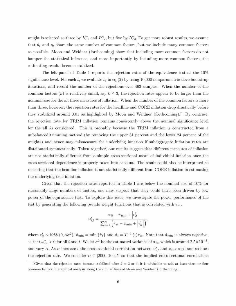
weight is selected as three by IC1 and IC2; but �ve by IC3: To get more robust results, we assume

that �t and �t share the same number of common factors, but we include many common factors

as possible. Moon and Weidner (forthcoming) show that including more common factors do not

hamper the statistical inference, and more importantly by including more common factors, the

estimating results become stablized.

The left panel of Table 1 reports the rejection rates of the equivalence test at the 10%

signi�cance level. For each t, we evaluate tz in eq.(2) by using 10,000 nonparametric sieve bootstrap

iterations, and record the number of the rejections over 463 samples. When the number of the

common factors (k) is relatively small, say k � 3, the rejection rates appear to be larger than thenominal size for the all three measures of in�ation. When the number of the common factors is more

than three, however, the rejection rates for the headline and CORE in�ation drop drastically before

they stabilized around 0.01 as highlighted by Moon and Weidner (forthcoming).7 By contrast,

the rejection rate for TRIM in�ation remains consistently above the nominal signi�cance level

for the all ks considered. This is probably because the TRIM in�ation is constructed from a

unbalanced trimming method (by removing the upper 31 percent and the lower 24 percent of the

weights) and hence may mismeasure the underlying in�ation if subaggregate in�ation rates are

distributed symmetrically. Taken together, our results suggest that di¤erent measures of in�ation

are not statistically di¤erent from a simple cross-sectional mean of individual in�ation once the

cross sectional dependence is properly taken into account. The result could also be interpreted as

re�ecting that the headline in�ation is not statistically di¤erent from CORE in�ation in estimating

the underlying true in�ation.

Given that the rejection rates reported in Table 1 are below the nominal size of 10% for

reasonably large numbers of factors, one may suspect that they could have been driven by low

power of the equivalence test. To explore this issue, we investigate the power performance of the

test by generating the following pseudo weight functions that is correlated with �it,

!�i;t =�it � �min +

����jit���Pni=1

��it � �min +

����jit���� ;where �jit � iidN (0; ��2); �min = min f�ig and �i = T�1

P�it. Note that �min is always negative,

so that !�i;t > 0 for all i and t:We let �2 be the estimated variance of �it; which is around 2.5�10�3;

and vary �: As � increases, the cross sectional correlation between !�i;t and �it drops and so does

the rejection rate. We consider � 2 [2000; 100; 5] so that the implied cross sectional correlations7Given that the rejection rates become stabilized after k = 3 or 4, it is advisable to add at least three or four

common factors in empirical analysis along the similar lines of Moon and Weidner (forthcoming).

6

between !�i;t and �it are approximately (0:030; 0:130; 0:482) ; respectively. The right panel of Table

1 reports the rejection rates of the pseudo in�ation rates at the 10% level for monthly in�ation.

Inspection of the table suggests that the discriminatory power is overall satisfactory, even when the

average cross sectional correlation (�) is as small as 0.03. This seems to suggest that the results in

Table 1 can hardly be viewed as an artifact of the low-power problem of the test.

In sum, our results in this section convincingly suggest that the PCE headline in�ation is not

statistically di¤erent from CORE or TRIM in�ation in consistently estimating the true underlying

in�ation (�t). At �rst, this comes as surprise in view of the fact that the relevant literature on

the appropriate measure of in�ation is largely split between studies that favor headline in�ation

and those that advocate the use of core in�ation. While the advocates of core in�ation claim that

the in�ation rates of food and energy are not in�uential to the true underlying in�ation but only

create noise, an obvious criticism of the focus on core in�ation is that it excludes the central items

to consumers like food and energy which are more related to their daily purchases (e.g., Bullard

2011). On one hand, our key �nding seems at odds with these con�icting views by not taking any

side, but on the other hand it can be usefully reconciled with both sides by asserting that the two

measures of in�ation are basically tracking the same underlying in�ation. Even if the prices of food

and energy items indeed capture the true underlying in�ation, core in�ation can still consistently

estimate the true underlying in�ation. To show this, let �fet denote the in�ation rate of the food and

energy which is assumed to follow the true underlying common factor, and n1 be the total number

of non-food and energy items. Then, the remaining individual in�ation rates can be written as

�cit = ai + �i�fet + �

coit ;

so that the weighted mean becomesnXi6=fe

!itPni6=fe !it

�cit =

nXi6=fe

!itPni6=fe !it

ai +

nXi6=fe

!itPni6=fe !it

�i�fet +

nXi6=fe

!itPni6=fe !it

�coit

= �+ ��fet +Op(n�1=21 )

! �+ ��fet as n1 !1:

Hence the weighted average of individual in�ation consistently captures the key underlying in�ation,

�fet ; even when �fet is excluded because all the other individual in�ation rates are closely linked to

the true underlying in�ation. That is, to the extent that individual in�ation rates follow a factor

model and that the true underlying in�ation is a function of the linear combination of common

factors, the probability limit of any weighted mean of in�ation becomes the true underlying in�ation

irrespective of the non-random weight functions.8

8 In a similar context, modeling the dynamics of in�ation within the structure of a common factor model, Stock

7

That being said, since our interpretation was mainly deduced from the fact that the expen-

diture weights in PCE data are not much correlated with individual in�ation rates, it is illuminating

to o¤er some intuitive explanations. A plausible explanation is that the substitution e¤ect of in-

dividual price changes is dominated by the income e¤ect. In that case, a lower price of a product

does not necessarily increase the PCE weight for the corresponding product unless the real ex-

penditure on the product increases more than the decrease in price. Consequently, the weights

of subcomponent in�ation will not vary much with individual price changes. Another possibility

is that the level of disaggregation of the PCE data is not �ne enough to capture the substitution

e¤ect satisfactorily. The PCE item of �New motor vehicles�, for instance, comprises cars of di¤erent

brands that are by nature close substitutes. If the price of a car rises and hence consumers switch

from one brand to another brand, the current PCE data cannot capture this substitution e¤ect

because they belong to the same item. If the substitution e¤ect mainly takes place within the PCE

product level, weights will not be responsive to the price changes of individual products.9

3 Out-of-sample forecasting performance

Another important issue is whether or not core in�ation is a better predictor of future headline

in�ation. Advocates of core in�ation often argue that core in�ation is more useful in forecasting

future headline in�ation probably because it measures the persistent or durable component of

headline in�ation. Before proceeding, it is instructive to brie�y discuss two popular approaches for

forecasting: recursive and rolling methods. While the recursive method utilizes all data observations

up to the forecasting point, the rolling regression method exploits a �xed number of observations at

each time. In consequence, the recursive method is known to perform better when the underlying

parameters are stable over time, whereas the rolling regression approach is preferred when structural

change or time-variation is suspected in the key parameters. To explore which approach is better

suited to our data, we plot in Figure 1 the AR(1) coe¢ cient estimates of the monthly PCE in�ation

rate (pt+1 � pt) with a 60-month rolling window. A visual inspection of Figure 1 favors the use ofthe rolling regression approach because the AR coe¢ cient estimates clearly exhibit time-varying

behavior, which cannot be e¤ectively captured by recursive regression.

and Watson (forthcoming) show that the forecasting performance based on the smoothed trend in�ation - which is

another estimate of the true underlying in�ation - is better than a simple random walk model.9Since the substitution e¤ect seems to hinge on the level of disaggregation, one might surmise that use of �ne

micro-level price data such as the ELI-level data adopted by Nakamura and Steinsson (2008) could change the key

results. This is an interesting avenue of research, but we leave it to future research it is beyond the scope of this

paper.

8

To substantiate this point, we plot in Figure 2 the squared forecast errors (SFE) of both

rolling and recursive regression methods which are estimated from the forecasting model shown in

eq.(6) below. Since the SFE of the rolling method tends to vary with the choice of rolling window

with poorer forecasting performance for longer rolling window, we set a rolling window of 60 months

at which the variance of SFE appears to stabilize. Not surprisingly, the SFE of the recursive method

is highly sensitive to the starting point of sample period. Moreover, the forecasting performance

of the recursive method becomes very poor when the sample includes the transition period from

the great in�ation to the great moderation in the 1970s and 80s, while the performance improves

greatly for the subsample periods after 1992 when in�ation has been relatively stable. This con�rms

our prior intuition that the recursive method is not appropriate for data with obvious structural

changes. Nevertheless, we �nd that forecasting based on the rolling regression outperforms the one

based on the recursive method in terms of the mean squared forecast error (MSFE) even for the

sample period beginning from 1992.M1. This validates our use of the rolling regression method in

evaluating the forecasting performance of di¤erent measures of in�ation.

3.1 Benchmark forecasting model

To compare the out-of-sample forecasting performance of the three measures of in�ation under

study, we consider the following benchmark forecasting model with 60-month rolling window for

the h-horizon. �ppce,t+h � ppce,t

12

�h = �h + �h (pjt � pjt�12) + �t+h;t; (6)

where pjt denotes price index of jth in�ation measure at t for j = fHeadline; CORE; TRIMg. Theleft-hand side of eq.(6) therefore represents the annualized PCE headline in�ation between t and

t+h with the h-month forecasting horizon. Note that in�ation rates are converted into percentage

changes. The corresponding mean squared forecasting error (MSFE) can then be obtained as

MSFE =1

P

To+PXt=To+1

�ppce,t+hjt � ppce,t+h

�2;

where To is the end of the sample used in the rolling estimation, and ppce,t+hjtis the �tted value

from eq.(6).

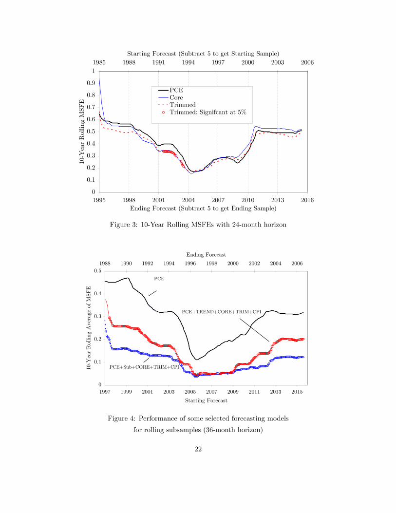
The results from this exercise are summarized in Figure 3 for the three measures of in�ation

under comparison. The thick solid line represents the average MSFEs for the PCE headline in�ation,

and the thin solid line and the dotted line respectively depict the average MSFEs for the CORE and

TRIM in�ation. Each point on the chart represents a 10-year average of the 60-month rolling MSFE

for the 24-month forecasting horizon. The numbers on the horizontal axis represent respectively

9

the beginning year (top) and the ending year (bottom) of each 10-year subsample period. For

instance, 1985 (top) and 1994 (bottom) on the horizontal axis capture the subsample period of

1985�1994, and so on. As in Crone et al. (2013), we assess the forecasting precision of the three

competing measures of underlying in�ation by reporting the Giacomini-White (2006) statistic for

testing whether there is a statistically signi�cant di¤erence in MSFEs between the models with

di¤erent measures of in�ation at the 5% signi�cance level.10 Any period in which the MSFEs of

headline in�ation are statistically di¤erent from those of TRIM in�ation is noted in symbols (circle).

A few things are of note from Figure 3. The �rst feature that is apparent in Figure 3 is

that the MSFEs of all three measures of in�ation takes on a U-shape pro�le over time, as they

decline initially but begins to rise back after the 1995-2004 subsample period. This largely mimics

the U-shaped pro�le seen in the AR coe¢ cient estimates in Figure 1, which is not surprising in

light of the close association between the forecasting error and the persistence of in�ation series.

Forecasting error is likely to be bigger (a larger MSFE) when in�ation series is more persistent (a

larger value of AR(1) coe¢ cient estimate).

Second, the CORE in�ation appears to outperform the PCE headline in�ation until around

2005. This con�rms the �ndings by earlier studies (e.g., Bryan et al. 1997, Clark 2001, Cogley

2002) that CORE in�ation is a better predictor of future headline in�ation. The outperformance

of the CORE in�ation, however, disappears quickly after 1996-2005 period when it is dominated by

the headline in�ation. This corroborates the recent �nding by Crone et al. (2013) who refute the

earlier �ndings based on a post-1990 dataset. Judging from the Giacomini-White�s (2006) statistics,

however, there is no statistically signi�cant di¤erence in the MSFE between the CORE in�ation

and the headline in�ation in the entire sample period considered. That is, there is no clear-cut

superiority between the two measures of in�ation in predicting future headline in�ation.

Third, a similar story is told when the headline in�ation is compared with the TRIM

in�ation, except for the subsample period of 1992 and 2003 when the MSFE of the TRIM in�ation

is signi�cantly smaller than that of the headline in�ation. Interestingly, this period coincides

with the data span studied by Clark (2001) who documents the dominance of the TRIM in�ation

over the headline in�ation in terms of forecasting precision. Other than this period, however, the

headline in�ation performs quite comparably, if not marginally better, in forecasting future headline

in�ation.10See eq.(3) in Crone et al. (2013,p.510) for the GW statistic.

10

3.2 Out-of-sample performance of competing forecasting models

The overall assessment of our results in the previous section is that headline in�ation is not out-

performed by CORE or TRIM in�ation in terms of forecasting accuracy. The results, however,

are not much informative about which speci�c forecasting model is better in predicting headline

in�ation. To address this issue, we conduct another set of exercise in a general multivariate fore-

casting model framework that encompasses conventional univariate models (e.g., Clark 2001) and

random-walk models (e.g., Stock and Watson forthcoming) to bivariate forecasting models (e.g.,

Crone et al. 2013). The novelty of our approach here is to extending the forecasting model to

a multivariate model that includes not only conventional regressors such CORE and TRIM, but

also subcomponents of PCE in�ation that received little attention in the literature. Although it is

widely agreed that in�ation forecasters have a dearth of reliable multivariate models for forecasting

in�ation, more recent studies (e.g., Crone et al. 2013) tend to suggest that forecasting performance

can be enhanced in a multivariate framework. Crone et al. (2013) also document that CPI in�ation

is helpful to enhance the precision of forecasting future headline in�ation. Since the forecasts from

the PCE headline in�ation per se are at least comparable to those from the alternative measures

of in�ation considered, we here focus on the headline PCE in�ation as a benchmark speci�cation.

To identify the best performing forecasting model, we consider the following general multi-

variate model speci�cation that nests many popular forecasting models of interest.�ppce;t+h � ppce;t

12

�h = �h + �h (pjt � pjt�12) +

kX`=1

`;h (x`;t � x`;t�12) + �t+h;t; (7)

where pjt denotes price index of j-th in�ation measure as before and x`t represents other price

variables such as CPI in�ation and subaggregate in�ation series for durable (D), nondurable (ND),

and service (S), dubbed as �Sub�throughout the paper. We also consider the principal component

estimated static common factors (PC, hereafter) as well as the smoothed trend with CORE (here-

after, TREND) which bears a close resemblance in spirit to the �multivariate UCSVO�discussed

in Stock and Watson (forthcoming).11 Note that the multivariate model in eq.(7) embraces (i)

random walk models (e.g., Stock and Watson 2007) when �h = 1;h = � � � = k;h = 0; (ii) single

regressor models (e.g., Clark 2001, Smith 2004) when 1;h = � � � = k;h = 0; and (iii) bivariate

regressor models (e.g., Crone et al. 2013) when 2;h = � � � = k;h = 0.11As an extension of the univariate unobserved components/stochastic volatility outlier-adjustment (UCSVO)

model that expresses the rate of in�ation as the sum of a permanent component (trend) and a transitory component,

the multivariate UCSVO (MUCSVO) model includes a common latent factor in both the trend and idiosyncratic

components of in�ation by allowing the factor loadings to vary over time. In this regard, the model with smooth

trended CORE considered in our analysis takes a similar structure with the MUCSVO.

11

For the multivariate models, we consider the following seven di¤erent model speci�cations

with various combinations of some key variables such as CORE, TRIM, CPI, Sub and TREND,

together with the PCE headline in�ation.12 As a result, the total number of models considered here

is 20 and the performance of each of these competing models is evaluated relative to the benchmark

model (BM) in eq.(6).

Case 1: PCE + Subs (ND, D and S) + CORE + TRIM + CPI

Case 2: PCE + PC + CORE + TRIM + CPI

Case 3: PCE + TREND + CORE + TRIM + CPI

Case 4: PCE + Sub + CORE + TRIM

Case 5: PCE + Sub + CORE

Case 6: PCE + Sub + TRIM

Case 7: Sub + CORE + TRIM

Table 2 reports the results of such an exercise with the forecasting horizons of h =24 and

36 months for the rolling window of 60 months.13 The �rst column of Table 2 presents the results

for the 24-month forecasting horizon and those for the 36-month horizon are reported in the third

column. The table displays a horse race of the forecasting errors that each of the 20 models make

in predicting future headline in�ation. Since the entries reported in the table are MSFEs from

corresponding forecasting models, forecasting models with lower values in the MSFE can be seen

as a better predictor of headline in�ation. The MSFEs with the smallest values are denoted in

bold-face.

The results in Table 2 illustrate several important points. First, as is obvious from the

table, all models make smaller errors in predicting headline in�ation when the forecasting hori-

zon is longer. Second, unlike the common perception built in the literature, multivariate models

appear to deliver signi�cantly more accurate forecasts of headline in�ation than their univariate

counterparts, lending credence to the recent �nding by Stock and Watson (forthcoming) and Crone

et al. (2013). It seems improbable that any one measure of in�ation alone has a signi�cant enough

forecasting power in predicting future headline in�ation. This �nding obviously runs counter to one

of the most robust �ndings from the empirical forecasting literature on the superiority of univariate

models to their multivariate counterparts. Among the seven multivariate models under study, the12The inclusion of the three sub-panels of headline in�ation as regressor is mainly guided by the number of common

factors chosen by using the Bai and Ng (2002)�s IC criteria. In addition to the three conventional product categories

of Durable (D), Non-Durable (ND) and Service (S), we also consider three sub-panels that are randomly selected

from 5,000 sub-panel combinations.13While the table only includes the results for the speci�c forecasting horizons, they are representative of the cases

for other horizons which are not reported to conserve the space.

12

model including both PCE headline in�ation and three sub-panels (ND, D and S) together with

CORE, TRIM and CPI in�ation performs the best. Third, a detailed review of Table 2 suggests

the combination of PCE and three sub-panels as superior regressors in predicting future headline

in�ation. Any forecasting models containing the combination appear to consistently outperform

those that do not, implying that those components are essential components in tracking the under-

lying in�ation. However, unlike Stock and Watson (forthcoming) and Crone et al. (2013), we fail to

�nd that including TREND in�ation or CPI in�ation alone improves the forecasting performance

of multivariate models.

Speaking of the role of three sub-panels, it is worth noting that we reach the same conclusion

on the best performing forecasting model even when three randomly generated sub-panels are used

in place of ND, D and S. As presented in the second column of the table, the average value of

MSFE obtained from 5,000 randomly generated combinations of three sub-panels (0.207 for �PCE

+ Sub�) is smaller than those from many other multivariate models under comparison. However, it

is still larger than that from the �All (sub)�model with the three conventional product categories as

sub-panels (0.167). Moreover, although the minimum value of MSFE from the randomly generated

sub-panels is slightly smaller than the case with the conventional large product categories, there

is no guarantee that the selected subpanels robustly outperform in di¤erent subsamples because

they are not consistently estimable. Our suggestion to practitioners is therefore to utilize the

three conventional sub-components of headline in�ation as the proxy for the common factors of

underlying in�ation. These conclusions carry over to the cases with 36-month forecasting horizon

which are presented in the right-hand side panel of Table 2.

The results in Table 2 illustrate already interesting points, but they are based on the entire

sample period. To ensure the robustness of our conclusions across subsample periods, we compare

the MSFEs of the two leading multivariate models, the one with �Sub�and the other with �TREND�,

for various sub-sample periods based on a rolling regression approach. Figure 4 displays the results

with the 36-month horizon, which are very similar to those outlined above in Table 2, clearly

demonstrating the dominance of the multivariate models relative to the benchmark model. Notice

that the 5% signi�cant cases that the MSFE from multivariate model is di¤erent from that of

the benckmark model are marked as a circle for the model with �PCE+Sub+CORE+TRIM+CPI�

and as a square for the model with �PCE+TREND+CORE+TRIM+CPI�. As displayed in Figure

4, the MSFEs of the best performing multivariate model with �PCE+Sub+CORE+TRIM+CPI�

are not only signi�cantly di¤erent from those of the benchmark model, but also are consistently

below those of the competing multivariate model with �TREND�in almost all subsample periods

considered. That is, our conclusions on the best performing forecasting model are fairly robust to

13

the choice of sample periods.

4 Conclusion

This paper makes two major arguments with regard to the much-debated issue on the measure

of in�ation for monetary policy purpose. First, the headline in�ation is not much statistically

di¤erent from CORE or TRIM in�ation in consistently tracking unobservable underlying in�ation.

Due to the lower volatility of the latter in practice, however, our results defend the use of CORE

in�ation as in Bryan and Cecchetti (1994). Second, when it comes to the choice of forecasting

model for predicting future headline in�ation, our results suggest that a multivariate model with

PCE headline in�ation and three sub-panels along with CORE, TRIM and CPI in�ation has the

best forecasting performance among 20 models under study. Its outperformance turns out to be

quite robust to the selection of sample periods.

14

References[1] Bai, Jushan and Serena Ng. (2002) �Determining the number of factors in approximate factor

models.�Econometrica, 70(1), 191-221.

[2] Bernanke, Ben S. and Mark Gertler. (1999) �Monetary policy and asset price volatility.�Federal Reserve Bank of Kansas City, Economic Review, 84 (Fourth Quarter), 17�51.

[3] Bickel, P.J. and E.L. Lehmann. (1975) �Descriptive statistics for nonparameteric models II.Location.�The Annals of Statistics, 3(5), 1045�1069.

[4] Bryan, Michael F., and Stephen G. Cecchetti. (1994) �Measuring Core In�ation.�In MonetaryPolicy, edited by N. Gregory Mankiw, pp.195�215. Chicago: University of Chicago Press.

[5] Bryan, Michael F., Stephen G. Cecchetti, and Rodney L. Wiggins II. (1997) �E¢ cient in�ationestimation.�NBER Working Papers No. 6183, National Bureau of Economic Research.

[6] Bullard, James. (2011) �Measuring In�ation: The Core is Rotten.�Federal Reserve Bank ofSt. Louis, Review, 93(4), 223�33.

[7] Chang, Yoosoon. (2004) �Bootstrap unit root tests in panels with cross-sectional dependency.�Journal of Econometrics, 120(2), 263�293.

[8] Clark, Todd. (2001) �Comparing Measures of Core In�ation.�Federal Reserve Bank of KansasCity, Economic Review, 86 (Second Quarter), 5�31.

[9] Cogley, Timothy. (2002) �A Simple Adaptive Measure of Core In�ation.�Journal of Money,Credit and Banking, 34(1), 94�113.

[10] Crone, Theodore M., N. Neil K. Khettry, Loretta J. Mester, and Jason A. Novak (2013) �CoreMeasures of In�ation as Predictors of Total In�ation.�Journal of Money, Credit and Banking,45(2-3), 505�519.

[11] Dolmas, Jim. (2009) �Excluding items from personal consumption expenditures in�ation,�Federal Reserve Bank of Dallas, Sta¤ Papers, No. 7, June.

[12] Giacomini, Ra¤aella and Halbert White. (2006) �Tests of Conditional Predictive Ability.�Econometrica, 74(6), 1545�1578.

[13] Mishkin, Frederic S. (2007) �Housing and the monetary transmission mechanism.�Board ofGovernors of the Federal Reserve System, Finance and Economics Discussion Series, 2007-40.

[14] Moon, Roger H. and Martin Weidner. (2015) �Linear Regression for Panel with UnknownNumber of Factors as Interactive Fixed E¤ects.�Econometrica, forthcoming.

[15] Nakamura, Emi and Jón Steinsson. (2008) �Five Facts about Prices: A Reevaluation of MenuCost Models.�Quarterly Journal of Economics 123, 1415�1464.

[16] Smith, Julie K. (2004) �Weighted Median In�ation: Is This Core In�ation?� Journal of Money,Credit and Banking, 36, 253�63.

[17] Stock, James H., and Mark W. Watson. (2007) �Has In�ation Become Harder to Forecast?�Journal of Money, Credit and Banking, 39, 3�33.

[18] Stock, James H., and Mark W. Watson. (2016) �Core In�ation and Trend In�ation.�Reviewof Economics and Statistics, forthcoming.

15

[19] Wynne, Mark A. (1999) �Core In�ation: A Review of Some Conceptual Issues.� FederalReserve Bank of Dallas, Review, research department working paper no. 99-03, June.

[20] Wynne, Mark A. (2008) �Core In�ation: A Review of Some Conceptual Issues.� FederalReserve Bank of St. Louis, Review, 90, 205�28.

16

Appendix

Appendix A: The sieve bootstrap procedure

Denote et = ["t; �t] where "t = ["1t; :::; "nt] ; �t = [�1t; :::; �nt] : Also de�ne �t = [mt; $t] wheremt = [m1t; :::; mkt]; $t = [$1t; :::; $kt]; and k is the assigned number of the common factors.

1. Estimate the sieve parameters: Constant terms (��i and �!i ) and AR(pi) coe¢ cients. To es-

timate the factor loading coe¢ cients, �rst standardize the in�ation rates and the �rst di¤er-enced log weights by their standard deviations, and then estimate the k largest eigen-vectorsof the n�n covariance matrixes (Principal Components (PC) estimators). The factor loadingcoe¢ cients can be estimated by running an individual in�ation rate (non-standardized series)on constant and the estimated PC factors.

2. Generate a (T +M) � 1 vector of random integers with the range of f1; :::; T � 24g : Drawthe pseudo errors from the residuals et and �t by selecting the entire n and k-dimensionalvectors to preserve the cross-sectional dependence.

3. Generate e�t from ��t using eq. (4) and (5). Discard the �rst M observations to avoid theinitial e¤ects. Here we set M = 200:

4. Re-center e�t and ��t : Subtract its time series mean to ensure that the pseudo error e

�it and �

�t

have zero means over t.

5. Generate ��it by combining �i + �0i��t with "

�it in eq. (3).

6. Construct ln!�it by taking cumulative sum of � ln!�it: Take exponential to get back !�it:

Standardize !�it.

7. Construct z�t by taking the di¤erence in the two pseudo weighted means.

8. Construct t-statistics, t�z = (z�t � zt) =

q��2z , where �

�2z is the bootstrapped variance.

9. Repeat the above steps (1 through 7) 10,000 times and construct the critical value at a givensigni�cance level.

Appendix B: Common factor estimationThe common factors are often estimated by using two popular approaches: principal component(PC) and cross-sectional averages of the subsamples. Under the assumption that individual in�ationfollows the following static factor model,

�it = ai + �0i�t + �

oit;

and the empirical common trend in�ation is de�ned as

� t =1

n

Xn

i=1ai +

1

n

Xn

i=1�0i�t;

where �t is an estimate of the common factors �t: Rather than including � t in the forecastingregression, we include �t directly in the forecasting regression because the direct inclusion improvesforecasting performance. The PC estimators are required the assumption of the stationarity of

17

�it;t+h meanwhile the cross sectional averages of the subpanels requires the stationarity of �oit.Since we assume that the number of the common factors is three, we split the 178 items into threesubpanels. And then we take the cross sectional averages to approximate the common factors. Let�pc

t and �cs

t be the PC and the cross sectional averages, respectively. Then it is straightforward toshow under the regularity conditions that

�pc

t = H 0�t +Op�C�1=2nT

�;

�cs

t = B0�t +Op�n�1=2

�:

where CnT = min [n; T ] ; H is an invertable (3� 3) rotating matrix and B is the (3� 3) matrix ofthe sample cross sectional averages �i for subpanels.

18

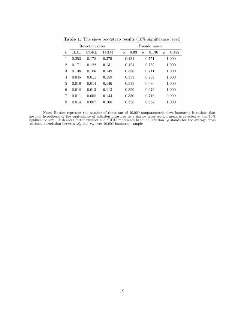
Table 1: The sieve bootstrap results (10% signi�cance level)

Rejection rates Pseudo power

k HDL CORE TRIM � = 0:03 � = 0:130 � = 0:482

1 0.253 0.178 0.379 0.431 0.751 1.000

2 0.171 0.122 0.131 0.424 0.739 1.000

3 0.138 0.106 0.149 0.386 0.711 1.000

4 0.045 0.011 0.159 0.373 0.739 1.000

5 0.010 0.014 0.146 0.333 0.686 1.000

6 0.018 0.013 0.113 0.359 0.673 1.000

7 0.011 0.008 0.144 0.330 0.716 0.999

8 0.014 0.007 0.166 0.328 0.654 1.000

Note: Entries represent the number of times out of 10,000 nonparametric sieve bootstrap iterations thatthe null hypothesis of the equivalence of in�ation measures to a simple cross-section mean is rejected at the 10%signi�cance level. k denotes factor number and �HDL�represents headline in�ation. � stands for the average crosssectional correlation between !�it and �it over 10,000 bootstrap sample

19

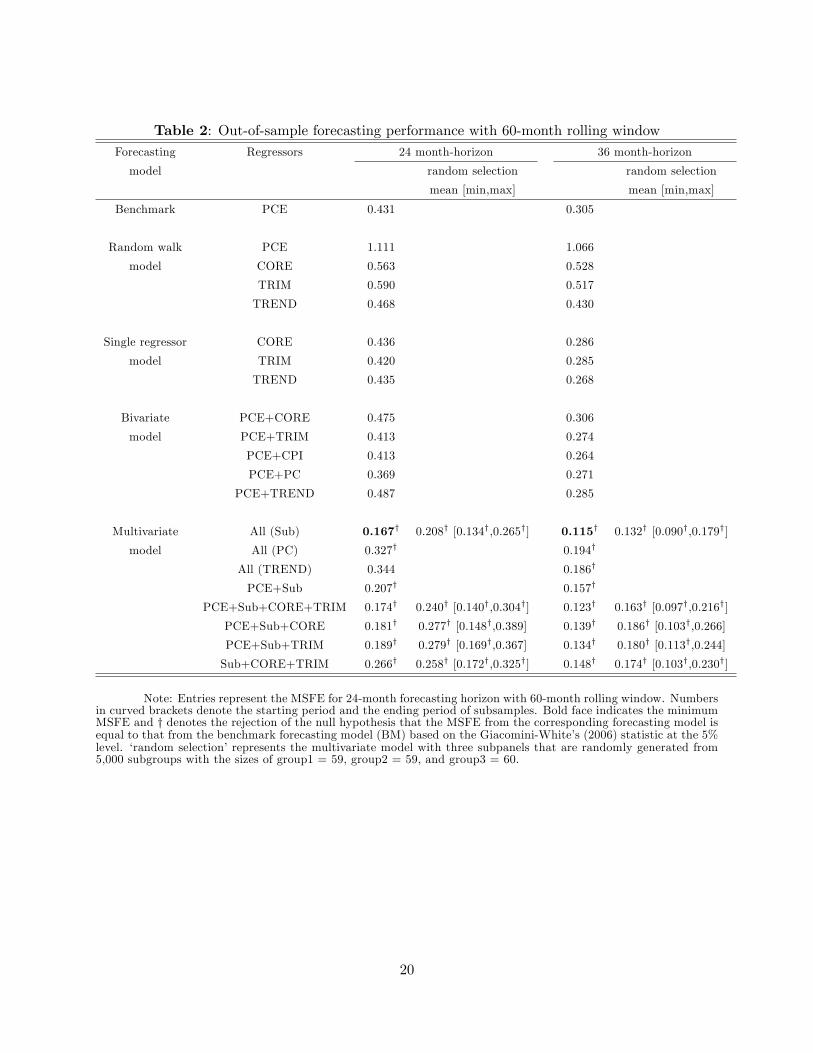
Table 2: Out-of-sample forecasting performance with 60-month rolling windowForecasting Regressors 24 month-horizon 36 month-horizon

model random selection random selection

mean [min,max] mean [min,max]

Benchmark PCE 0.431 0.305

Random walk PCE 1.111 1.066

model CORE 0.563 0.528

TRIM 0.590 0.517

TREND 0.468 0.430

Single regressor CORE 0.436 0.286

model TRIM 0.420 0.285

TREND 0.435 0.268

Bivariate PCE+CORE 0.475 0.306

model PCE+TRIM 0.413 0.274

PCE+CPI 0.413 0.264

PCE+PC 0.369 0.271

PCE+TREND 0.487 0.285

Multivariate All (Sub) 0.167y 0.208y [0.134y,0.265y] 0.115y 0.132y [0.090y,0.179y]

model All (PC) 0.327y 0.194y

All (TREND) 0.344 0.186y

PCE+Sub 0.207y 0.157y

PCE+Sub+CORE+TRIM 0.174y 0.240y [0.140y,0.304y] 0.123y 0.163y [0.097y,0.216y]

PCE+Sub+CORE 0.181y 0.277y [0.148y,0.389] 0.139y 0.186y [0.103y,0.266]

PCE+Sub+TRIM 0.189y 0.279y [0.169y,0.367] 0.134y 0.180y [0.113y,0.244]

Sub+CORE+TRIM 0.266y 0.258y [0.172y,0.325y] 0.148y 0.174y [0.103y,0.230y]

Note: Entries represent the MSFE for 24-month forecasting horizon with 60-month rolling window. Numbersin curved brackets denote the starting period and the ending period of subsamples. Bold face indicates the minimumMSFE and y denotes the rejection of the null hypothesis that the MSFE from the corresponding forecasting model isequal to that from the benchmark forecasting model (BM) based on the Giacomini-White�s (2006) statistic at the 5%level. �random selection�represents the multivariate model with three subpanels that are randomly generated from5,000 subgroups with the sizes of group1 = 59, group2 = 59, and group3 = 60.

20

0

0.1

0.2

0.3

0.4

0.5

0.6

0.7

0.8

1987 1992 1997 2002 2007 2012 2017

Ending Sample

Est

imate

 fro

m t

he 

Rollin

g R

egre

ssio

n

1977 1982 1987 1992 1997 2002 2007

Starting Sample

Figure 1: Rolling Estimated AR(1) Parameters with Monthly PCE In�ation

0

1

2

3

4

5

6

1986 1991 1996 2001 2006 2011 2016

Forecasts

Square

s of Fore

cast

 Err

ors

60­month rolling forecast

Recursive forecast (starting from 1977.M2)

Recursive forecast (starting from 1992.M1)

Figure 2: The Rolling and Recurisve MSFEs with 36-month Horizon

21

0

0.1

0.2

0.3

0.4

0.5

0.6

0.7

0.8

0.9

1

1995 1998 2001 2004 2007 2010 2013 2016

Ending Forecast (Subtract 5 to get Ending Sample)

10­Y

ear 

Rollin

g M

SFE

1985 1988 1991 1994 1997 2000 2003 2006

Starting Forecast (Subtract 5 to get Starting Sample)

PCECoreTrimmedTrimmed: Signifcant at 5%

Figure 3: 10-Year Rolling MSFEs with 24-month horizon

0

0.1

0.2

0.3

0.4

0.5

1997 1999 2001 2003 2005 2007 2009 2011 2013 2015

Starting Forecast

10­Y

ear 

Rollin

g A

ver

age 

of M

SFE

1988 1990 1992 1994 1996 1998 2000 2002 2004 2006

Ending Forecast

PCE

PCE+TREND+CORE+TRIM+CPI

PCE+Sub+CORE+TRIM+CPI

Figure 4: Performance of some selected forecasting models

for rolling subsamples (36-month horizon)

22