retrieving sea surface salinity with multiangular l-band

Retrieving sea surface salinity with multiangular L-band

brightness temperatures: Improvement by spatiotemporal

averaging

A. Camps, M. Vall-llossera, L. Batres, F. Torres, N. Duffo, and I. Corbella

Department of Signal Theory and Communications, Universitat Politecnica de Catalunya, Barcelona, Spain

Received 4 February 2004; revised 30 August 2004; accepted 3 January 2005; published 31 March 2005.

[1] The Soil Moisture and Ocean Salinity (SMOS) mission was selected in May 1999 bythe European Space Agency to provide global and frequent soil moisture and sea surfacesalinity maps. SMOS’ single payload is Microwave Imaging Radiometer by ApertureSynthesis (MIRAS), an L band two-dimensional aperture synthesis interferometricradiometer with multiangular observation capabilities. Most geophysical parameterretrieval errors studies have assumed the independence of measurements both in time andspace so that the standard deviation of the retrieval errors decreases with the inverse ofsquare root of the number of measurements being averaged. This assumption is especiallycritical in the case of sea surface salinity (SSS), where spatiotemporal averaging isrequired to achieve the ultimate goal of 0.1 psu error. This work presents a detailed studyof the SSS error reduction by spatiotemporal averaging, using the SMOS end-to-endperformance simulator (SEPS), including thermal noise, all instrumental error sources,current error correction and image reconstruction algorithms, and correction ofatmospheric and sky noises. The most important error sources are the biases that appear inthe brightness temperature images. Three different sources of biases have beenidentified: errors in the noise injection radiometers, Sun contributions to the antennatemperature, and imaging under aliasing conditions. A calibration technique has beendevised to correct these biases prior to the SSS retrieval at each satellite overpass.Simulation results show a retrieved salinity error of 0.2 psu in warm open ocean, and up to0.7 psu at high latitudes and near the coast, where the external calibration method presentsmore difficulties.

Citation: Camps, A., M. Vall-llossera, L. Batres, F. Torres, N. Duffo, and I. Corbella (2005), Retrieving sea surface salinity

with multiangular L-band brightness temperatures: Improvement by spatiotemporal averaging, Radio Sci., 40, RS2003,

doi:10.1029/2004RS003040.

1. Introduction

[2] The scientific objectives of the SMOS mission arelisted in Table 1. These objectives can be achieved bymicrowave radiometry at L band. However, real apertureradiometers require antennas of several meters in diam-eter to achieve the required spatial resolution from space.To overcome this problem, SMOS exploits for the firsttime in Earth observation from space, the 2-D aperturesynthesis interferometric radiometry concept used fordecades in radiastronomy [Thompson et al., 1986].

[3] The data processing involved to obtain a brightnesstemperature image is complex and includes detailedinstrument modeling of receivers [Torres et al., 1997]and antennas [Camps et al., 1997b, 1998b], error cor-rection by distributed noise injection [Torres et al., 1996;Corbella et al., 1998], and image reconstruction algo-rithms [Camps et al., 1998a, 2004b]. In the ideal case ofidentical receivers and antenna voltage patterns, andnegligible spatial decorrelation effects, the relationshipbetween the samples of the so-called ‘‘visibility func-tion’’ (obtained from the cross-correlation products of thesignals collected by each pair of receiving elements) andthe brightness temperature images (Tx and Ty in theantenna reference frame) expressed in the directioncosines domain (x, h) = (sin q cos j, sin q sin j) reduces

RADIO SCIENCE, VOL. 40, RS2003, doi:10.1029/2004RS003040, 2005

Copyright 2005 by the American Geophysical Union.

0048-6604/05/2004RS003040$11.00

RS2003 1 of 13

to a Fourier transform. The samples of the visibilityfunction are measured by the interferometric radiometerat a set of spatial wave numbers (u, v) determined by thespacing between the pair of antennas normalized to thewavelength: (u, v) = (x2 � x1, y2 � y1)/l.[4] In SMOS the antennas are distributed along three

arms 120� apart and are spaced d = 0.875 wavelengths(Figure 1a). However, the Nyquist criterion for hexago-nal sampling requires that the antenna separation be d =1/

ffiffiffi3

pwavelengths to avoid aliasing in the unit circle

(x2 + h2 = 1) [Camps et al., 1997a]. Therefore thereconstructed 2-D brightness temperature images sufferfrom aliasing and replicas of the Earth image (‘‘aliases’’)overlap with the Earth image in the fundamental period(Figure 1b), which defines the alias-free field of view(AF-FOV). Each pixel in the AF-FOV is seen at adifferent incidence angle, radiometric sensitivity, andspatial resolution (Figure 1c). As the satellite moves,the projection of the AF-FOV in cross-track/along-trackEarth coordinates is displaced from snapshot to snap-shot, and pixels are then seen in different positions in theAF-FOV at different incidence angles. Figure 1b repre-sents the equi-incidence angle contours in the AF-FOVas shown in the work of Camps et al. [2003a, 2003b].[5] As in the work of Camps et al. [2003a], the SSS

retrieval algorithm is stated as a minimization problem ofthe mean squared error between the measured firstStokes parameter (computed as the sum of the brightnesstemperature images at both polarizations measured in theantenna reference frame and the one modeled usingestimated parameters for all pixels within the swathwidth (Figure 2). (Existing measurements and theoreticalpredictions show that the third Stokes parameters at Land is negligible.)

e ¼ 1

Nobservations

XNobservations

n¼1

� Imodeln qn;U10; SST; SSS� �

� Idatan

� �2 t q;fð Þcos q

� �: ð1Þ

The parameters to be recovered are the sea surfacesalinity (SSS), the sea surface temperature (SST), and theeffective 10 m height wind speed (U10), which accountsfor sea state effects (wind-induced waves, swell, etc.) andnot just the waves induced by the wind. This procedurehas shown a better performance than having SST and U10

constant with a value equal to the ancillary data providedby other instruments [Gabarro et al., 2003]. Since In

data

are independent, the covariance matrix is diagonal, andonly the terms t(q, f) (average normalized antennaradiation pattern of all receiving elements) and cos q =ffiffiffiffiffiffiffiffiffiffiffiffiffiffiffiffiffiffiffiffiffiffiffi

1� x2 � h2p

(obliquity factor) are needed to weight theradiometric measurements according to the noise in each

pixel of the 2-D brightness temperature image. Thenumber Nobservations is the number of measurementsacquired of the same location (pixel) in a satelliteoverpass, and it is determined by the satellite’s groundspeed and the length of the dwell line (maximumdistance in the AF-FOV in the along-track direction).Owing to the instrument’s limited angular resolution,Earth ‘‘aliases’’ enter in the nominal AF-FOV. (MIRAS’angular resolution is 2.25� if the visibility samples aretapered with a Blackman window prior to the imagereconstruction.) Contribution from Earth aliases isnegligible if a guard region of width �1.5� (or Dx =0.026) is kept, which also reduces slightly the maximumswath width. Figure 2 presents the pixels that are imagedfor the first time in an overpass. As the distance to theground track (abscissa in Figure 1c) increases, thenumber of observations decreases (length of dwell lineshortens) and measurements become noisier (Figure 1c)due to the antenna pattern and obliquity factorcompensation in the image reconstruction process, whichincreases the magnitude of the retrieved parameter errors.This effect is seen more clearly in the series of simulatedbrightness temperature observations over the Earth fordifferent cross-track distances to the satellite’s groundtrack (Figures 3a–3f). The number of observationsincreases as the dwell line approaches the ground track,reaching a maximum around the cross-track position250 km and then slightly decreases again. In addition,each observation is acquired at a different incidenceangle, and pixels in dwell lines close to the ground trackare imaged twice at the same incidence angle in the foreand aft directions (Figure 3f).[6] The minimization of equation (1) is performed

using a recurrent Levenberg-Marquardt least squares fit[Press et al., 1992]. Without loss of generality, the firstguess values are assumed to be ancillary data from othersensors, and the search limits are determined by typicalsensors’ errors: SSTancillary� 0.3�C�SST� SSTancillary +0.3�C and U10 ancillary � 2.5 m/s � U10 � U10 ancillary +

Table 1. Main Scientific Objectives of the SMOS Mission

Scientific Objectives Requirements

OceanGlobal sea surface salinitymaps

0.1 psu every 10–30 days

200 km spatial resolution

LandGlobal soil moisture 0.035 m3/m3 every 3 daysVegetation water contentmaps

0.2 kg/m2

Cryosphere (experimental) 60 km spatial resolutionimproved snow mantlemonitoring andmultilayer ice structure.

RS2003 CAMPS ET AL.: SALINITY RETRIEVAL AND AVERAGING

2 of 13

RS2003

2.5 m/s. In the case of sea surface salinity, no a prioriinformation has been used except the minimum andmaximum values found in the oceans and open seas:28 psu � SSS � 40 psu.

[7] The proposed approach has the following advan-tages [Camps et al., 2003a]: (1) avoids the singularitiesin the transformation from the antenna (Tx, Ty) to theEarth (Th, Tv) reference frames [Waldteufel and Caudal,

Figure 1. (a) SMOS payload module phase B configuration (courtesy of EADS-CASA Espacio,Spain). (b) SMOS observation geometry. Half-space is mapped into the unit circle in (x, h)coordinates. The alias-free field of view (FOV) that is imaged by the instrument is marked in lightgray is enlarged up to the Earth ‘‘aliases’’ limit by taking into account the sky contribution.(c) Incidence angle (dashed lines from 10� to 60�, circles centered at (0, 0)); spatial resolution(dash-dot lines from 40 to 80 km, best spatial resolution 32 km); and radiometric sensitivity (dottedlines from 4 to 6 K, best radiometric sensitivity �2.4 K if all available redundancies used and�3.6 K if not).


3 of 13

RS2003

2002] since Imeasured = Tx + Ty = Th + Tv; (2) avoids theFaraday rotation correction; (3) minimizes the angulardependence of the difference between the emissivitiescomputed with different dielectric constant models(e.g., Klein and Swift [1977] or Ellison et al. [1998];see Camps et al. [2003a, Figure 4]); and (4) minimizesthe emissivity angular dependence induced by otherfactors as the swell [Miranda et al., 2003] (notaccounted for in equation (1) but found in actualmeasurements).[8] This study is organized as follows. Section 2

explains the atmospheric and sky radiometric correctionsthat have to be applied. Section 3 details the originof different sources of bias in the brightness temper-ature images and explains an external calibrationtechnique devised to compensate them and get usefulSSS estimates. Section 4 presents a complete set ofsimulation results of the techniques presented usingthe SEPS with high spatial (geophysical data maps at1/16 of degree) and temporal resolution (daily vari-ation) covering a whole period of 30 days. These

results are used to analyze the improvement factorby spatial and temporal averaging. Finally, section 5summarizes the main results: the conditions forproper operation of the proposed external calibration,and the error reduction expected by spatiotemporalaveraging.

2. Radiometric Correction of Brightness

Temperature Images on Top of the

Atmosphere

[9] The brightness temperature models in the SMOSend-to-end performance simulator include many geo-physical parameters from the atmosphere, the sea,the land and the ionosphere [Camps et al., 1997c;Corbella et al., 2003; Camps et al., 2003b]. (Thegeophysical parameters used in SEPS are as follows:atmospheric liquid water and rain rate; land, snow, andvegetation albedos; soil surface temperature, moisture,and roughness; vegetation height, snow depth, seasurface salinity, temperature, wind speed, and ice coverfraction; as well as the galactic noise map, the inter-national reference ionosphere, and the internationalgeomagnetic reference field model to model the iono-sphere and the Faraday rotation.) Therefore, beforeapplying the SSS retrieval algorithm (equation (1)) anumber of radiometric corrections must be performedto derive the first Stokes parameter over the Earth’ssurface (Idata in equation (1)) from the apparent bright-ness temperatures measured by the instrument on topof the atmosphere (Imeasured = Tx + Ty):

Idata|{z}I referred to

Earth0s surface

¼ Tx þ Ty

� �|fflfflfflfflfflffl{zfflfflfflfflfflffl}I measured on

Top Of Atmosphere ðTOAÞ

� L qð Þ � Gh qð Þ þ Gv qð Þð ÞTSKY

L qð Þ

�þTUP atm qð ÞL qð Þ

�

� Gh qð Þ þ Gv qð Þð ÞTDN atm qð Þ; ð2Þ

to account for the upwelling atmospheric noise (TUP atm),and the downwelling atmospheric noise (TDN atm) andthe cosmic and galactic noises (TSKY) that are scatteredover the Earth’s surface. In equation (2) L = Latm +Lion � Latm (>1) is the total attenuation (atmosphere +ionosphere) and Gh,v(q) is the effective reflectivity of thesea surface at horizontal or vertical polarizations, and qis the incidence angle. The effective reflectivity of thesea surface is computed as Gh,v(q) = 1 � eh,v(q), whereeh,v(q) is an estimate of the sea surface’s emissivity

Figure 2. Evolution of nadir pixels in along-track/cross-track coordinates (gray dots at cross track = 0 km).Hexagonal-like contours indicate the position of the first(solid line) and last (dashed line) alias-free field of views.Black dots, pixels under study covering the whole swathup to the guard pixels the first time they are seen in anoverpass.


4 of 13

RS2003

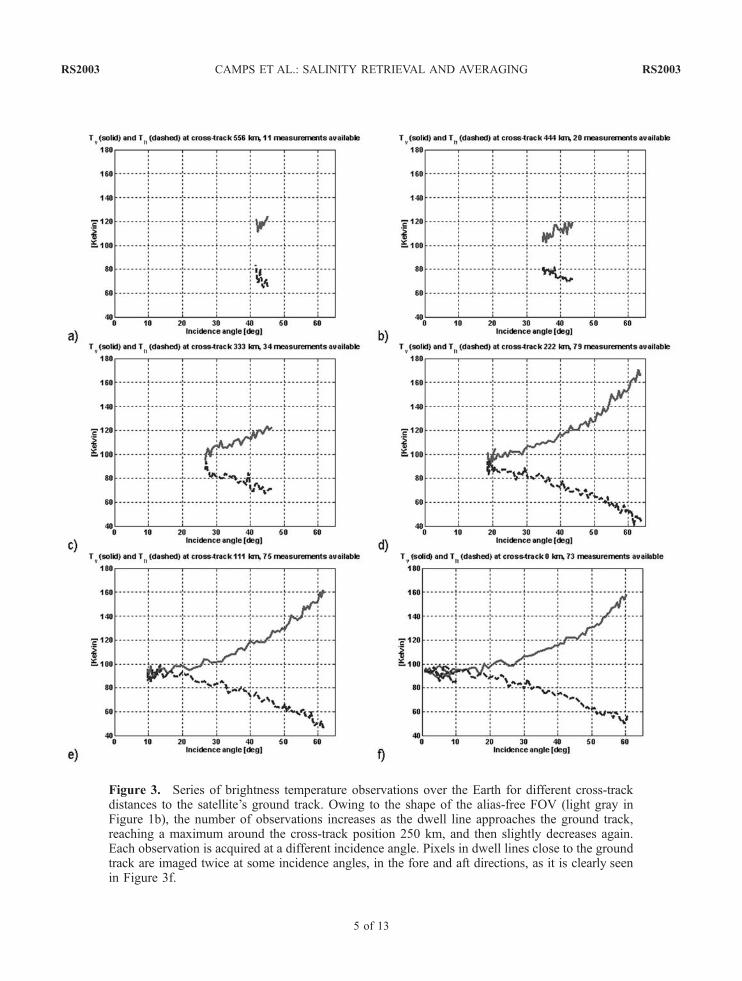
Figure 3. Series of brightness temperature observations over the Earth for different cross-trackdistances to the satellite’s ground track. Owing to the shape of the alias-free FOV (light gray inFigure 1b), the number of observations increases as the dwell line approaches the ground track,reaching a maximum around the cross-track position 250 km, and then slightly decreases again.Each observation is acquired at a different incidence angle. Pixels in dwell lines close to the groundtrack are imaged twice at some incidence angles, in the fore and aft dir ections, as it is clearly seenin Figure 3f.


5 of 13

RS2003

(equation (3)), which is computed from Gh,vspecular, the

square of the module of the Fresnel reflection coeffi-cient, and the ancillary data:

eh � 1� Gspecularh SSTancillary; SSSancillary; q

� � �

þ 0:2 1þ q55�

� �U10 ancillary

SSTancillary

; ð3aÞ

ev � 1� Gspecularv SSTancillary; SSSancillary; q

� �� þ 0:2 1� q

55�

� �U10 ancillary

SSTancillary

: ð3bÞ

Ancillary data used in the simulations are as follows: seasurface temperature (SSTancillary), sea surface salinity(SSSancillary), and wind speed (U10 ancillary). Sea state ismodeled by a simple linear fit to Hollinger’s data[Hollinger, 1971] with U10 as parameter. Other effectsare neglected. More recent measurements [Camps et al.,2003a, 2004a] have found new values for the wind-dependent terms in equations (3a) and (3b). Within themeasurements error bars, these values can be fitted by alinear expressions as in equations (3a) and (3b), withslightly different parameters. In the present study thecorrection terms in equation (2) are assumed to be atzenith equal to: TUP atm � 1.86 K, TDN atm � 2.10 K[Goodberlet and Miller, 1997], and L � Latm �0.0402 dB. Off-zenith, to account for the actual atmo-spheric path due to Earth’s curvature, these values aredivided by the cosine of an equivalent incidence angle:

cos qeq ¼hatmffiffiffiffiffiffiffiffiffiffiffiffiffiffiffiffiffiffiffiffiffiffiffiffiffiffiffiffiffiffiffiffiffiffiffiffiffiffiffiffiffiffiffiffiffiffiffiffiffiffiffiffiffiffiffiffiffiffiffiffi

R2T cos

2 qð Þ þ hatm þ 2RTð Þhatmq

� RT cos qð Þ;

ð4Þ

where hatm is the atmosphere height, and RT is theEarth’s radius.[10] Last, the sky (cosmic+galactic) noise in equation (2)

is estimated from satellite’s position, attitude, time, andthe 1420 MHz sky map [Reich, 1982; Reich and Reich,1986] (see also http://skyview.gsfc.nasa.gov/) as de-scribed in the work of LeVine and Abraham [2004].[11] It should be pointed out that in this simplified

model: (1) the azimuthal signature of eh and ev has beenneglected since to date no field experiments have pro-vided an evidence of it within the measurement accuracy(±0.1 K), except in very particular cases [Camps et al.,2004a]; (2) equations (3a) and (3b) represent the first-order Taylor’s expansion of eh(U10) and ev(U10), which isvery accurate at L band for wind speeds in the range 2–18 m/s [Etcheto et al., 2004, Figure 8]; and (3) in thescattered terms (Gh(q) + Gv(q))TSKY/L(q) and (Gh(q) +

Gv(q))TDN atm(q) only the specular reflection terms areconsidered.

3. External Calibration of the Brightness

Temperature Images

[12] The properties of the brightness temperatureimages obtained from SEPS exhibit an excellent agree-ment with the SMOS error budget predictions in terms ofradiometric accuracy and sensitivity [Camps et al.,2003c]. However, when comparing these images withrespect to the ideal ones (same angular resolution butwithout noise and instrumental errors), there is often abias. Three sources of bias have been identified:[13] 1. Instrumental inaccuracies in the noise injec-

tion radiometers (NIRs) used to measure the antennatemperature (average value of the scene). These errorsare: thermal noise (DT�0.2 K), offset, and linearityerrors. While the offset causes a scene-independentbrightness temperature bias, the linearity error causesa brightness temperature error, which is dependent on theantenna temperature corresponding to the scene beingimaged. These terms are also temperature-dependent andtherefore depend on satellite’s argument of the latitude.[14] 2. Inherent difference between the antenna tem-

perature (average value of the brightness temperature ofthe scene in the unit circle) and the average brightnesstemperature in the AF-FOV (Figure 1b) since the AF-FOV does not cover the whole space. This error has beenfound to be more important in inhomogeneous scenes(e.g., near the coastline).[15] 3. Sun contribution to the antenna temperature.

Even though some image reconstruction algorithmsinclude Sun brightness temperature estimators and can-cellators such as Camps et al. [2004b], Sun cancellationis never perfect and there is always a residual error whichappears as ripples (‘‘tails’’ of the quasi-impulse response)and a residual contribution to the antenna temperature.[16] If the sensitivity of the brightness temperature at

nadir to the sea surface salinity is DT/DSSS � 0.5 K/psuat 25�C (even smaller at lower temperatures) and the goalis to achieve an SSS error of 0.1 psu, the absoluteaccuracy of a real aperture radiometer should be 0.05 K,which is very challenging for any type of radiometer. Thislevel of accuracy is very unlikely in a MIRAS-type ofinstrument with internal calibration only [Torres et al.,1996; Corbella et al., 1998], and therefore some sort ofexternal calibration must be envisaged.[17] The use of one or several tie points to match the

retrieved brightness temperature does not produce satis-factory results since the radiometric sensitivity ofMIRAS is �2.4 K at boresight, and worsens away fromthis direction [Camps et al., 2004c]. The proposedexternal calibration technique relies on the use of ancil-


6 of 13

RS2003

lary SST and U10 data, and SSS estimates to predict thebrightness temperature of nadir pixels (0� incidenceangle, gray dots in Figure 2), for all the snapshot imagescontaining the pixels where the SSS is going to beretrieved (pixels marked as black dots the first time theyare seen in an overpass, Figure 2). For the whole series ofsnapshots, the nadir brightness temperatures at bothpolarizations are added together to form the estimatedfirst Stokes parameter at nadir (In), and finally, the Invalues corresponding to each snapshot are then averagedto reduce its noise (Figure 2):

�I ¼ 1

Nobservations

XNobservations

n¼1

In ¼1

Nobservations

XNobservations

n¼1

� TmodelBh q ¼ 0�; SSTancillary; SSSancillary;U10 ancillary

�n

��

þ TmodelBv

�q ¼ 0�;SSTancillary;SSSancillary;U10 ancillary

�n

�;

ð5Þ

The same procedure is followed with the measured data.Finally, the average bias for the set of snapshots used inthe retrieval is computed as

DI ¼ �Idata � �

I; ð6Þ

which is then subtracted from Indata, for all image pixels in

equation (1), and for all the snapshots in which the pixelis visible.

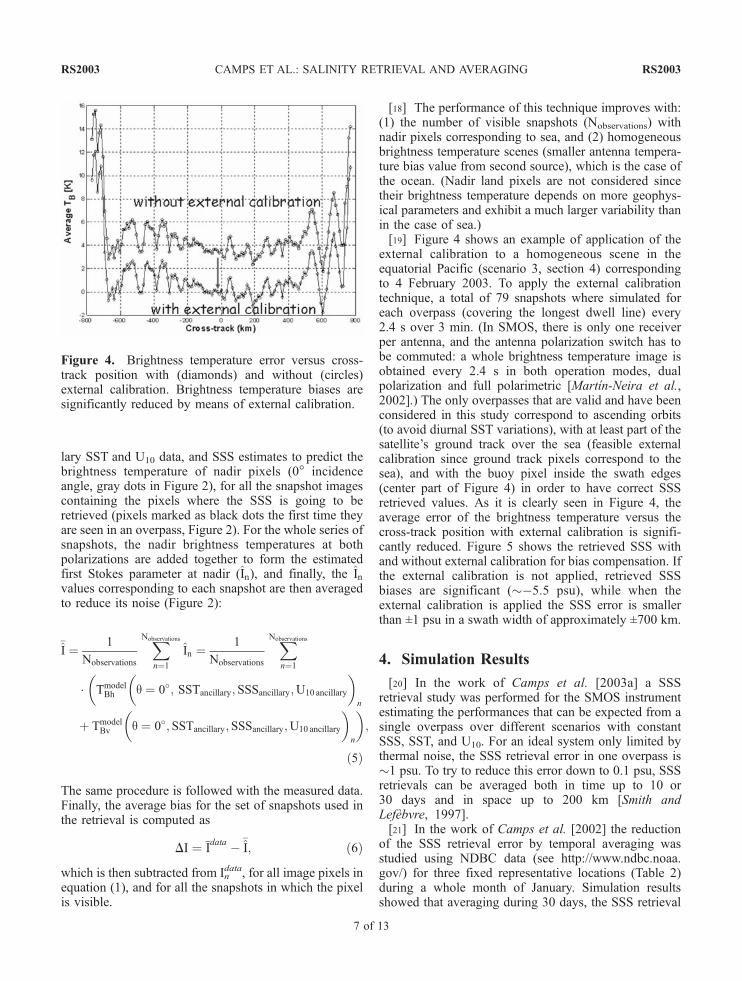
[18] The performance of this technique improves with:(1) the number of visible snapshots (Nobservations) withnadir pixels corresponding to sea, and (2) homogeneousbrightness temperature scenes (smaller antenna tempera-ture bias value from second source), which is the case ofthe ocean. (Nadir land pixels are not considered sincetheir brightness temperature depends on more geophys-ical parameters and exhibit a much larger variability thanin the case of sea.)[19] Figure 4 shows an example of application of the

external calibration to a homogeneous scene in theequatorial Pacific (scenario 3, section 4) correspondingto 4 February 2003. To apply the external calibrationtechnique, a total of 79 snapshots where simulated foreach overpass (covering the longest dwell line) every2.4 s over 3 min. (In SMOS, there is only one receiverper antenna, and the antenna polarization switch has tobe commuted: a whole brightness temperature image isobtained every 2.4 s in both operation modes, dualpolarization and full polarimetric [Martın-Neira et al.,2002].) The only overpasses that are valid and have beenconsidered in this study correspond to ascending orbits(to avoid diurnal SST variations), with at least part of thesatellite’s ground track over the sea (feasible externalcalibration since ground track pixels correspond to thesea), and with the buoy pixel inside the swath edges(center part of Figure 4) in order to have correct SSSretrieved values. As it is clearly seen in Figure 4, theaverage error of the brightness temperature versus thecross-track position with external calibration is signifi-cantly reduced. Figure 5 shows the retrieved SSS withand without external calibration for bias compensation. Ifthe external calibration is not applied, retrieved SSSbiases are significant (��5.5 psu), while when theexternal calibration is applied the SSS error is smallerthan ±1 psu in a swath width of approximately ±700 km.

4. Simulation Results

[20] In the work of Camps et al. [2003a] a SSSretrieval study was performed for the SMOS instrumentestimating the performances that can be expected from asingle overpass over different scenarios with constantSSS, SST, and U10. For an ideal system only limited bythermal noise, the SSS retrieval error in one overpass is�1 psu. To try to reduce this error down to 0.1 psu, SSSretrievals can be averaged both in time up to 10 or30 days and in space up to 200 km [Smith andLefebvre, 1997].[21] In the work of Camps et al. [2002] the reduction

of the SSS retrieval error by temporal averaging wasstudied using NDBC data (see http://www.ndbc.noaa.gov/) for three fixed representative locations (Table 2)during a whole month of January. Simulation resultsshowed that averaging during 30 days, the SSS retrieval

Figure 4. Brightness temperature error versus cross-track position with (diamonds) and without (circles)external calibration. Brightness temperature biases aresignificantly reduced by means of external calibration.


7 of 13

RS2003

error ranged from 0.12 psu to 1.06 psu, depending on thescenario location and the meteorological/oceanographicconditions. The impact of geophysical modeling errorsand biases in the first Stokes parameter were also

analyzed, indicating a maximum allowable bias ofjIbiasj < 0.22 K to achieve the 0.1 psu goal.[22] In this study the SSS error reduction by spatial

averaging is analyzed at four different levels: SMOS

Figure 5. (a and b) Sea surface salinity retrieval without and (c and d) with external calibration,retrieved sea surface salinity (Figures 5a and 5b), and sea surface salinity error (Figures 5c and 5d).

Table 2. Number of Satellite Overpasses for Each Scenarioa

ScenarioReferenceBuoy Location

DescendingOrbits

Ground TrackPixels = Land

Location atSwath Edge

ValidOverpasses

1 station 46184,North Nomad

53.91�N,138.85�W(coast of Alaska)

51 9 4 39

2 station 41025,Diamond Shoals

35.15�N,75.29�W(coast of North Carolina)

27 4 2 14

3 station 51028,Christmas Island DWA

0.00�N,153.88�W(equatorial Pacific)

28 0 4 24

aThe present study has only considered overpasses in ascending orbits, with valid external calibration (external calibration pixels = ocean pixels),and with the reference SMOS pixel outside the swath edges to provide correct SSS retrieved values.


8 of 13

RS2003

pixel size (�30 km, varying with pixel location in theAF-FOV), 50 km, 100 km, and 200 km. The errorreduction by temporal averaging is then also studied inperiods of 10 or 30 days. The global data used in SEPS[Meeson et al., 1995] are at 1� � 1� resolution, whichcorresponds to �110 km at the equator, larger than theSMOS spatial resolution. Therefore, in order to be ableto study the improvement by spatial averaging, SSS,SST, and U10 input data is needed for the SEPS bright-ness temperature generator at a spatial resolution higherthan the best SMOS spatial resolution [Camps et al.,2003b]. The SST and U10 input data were provided bythe Naval Research Laboratory (NRL) as outputs of thelayered ocean model (see http://www7320.nrlssc.navy.mil/global_nlom/) at a spatial resolution of 1�/16 and adaily variation covering a whole period of 30 days from14 January to 13 February 2003. The only SSS dataavailable were the original Levitus data at 1� resolution.However, taking into account that the SMOS revisit timeis 3 days at the equator, small-scale (�7 km at theequator) and temporal (1 day) variabilities are retainedsince they are mostly induced by the wind fields. Only athigh latitudes, the temporal variability is lost (revisit time<1 day), but some randomness is kept owing to instru-

mental noise and the changing position of the pixelunder observation in the swath.[23] The average values of the SSS, SST, and U10

for the period under study in the reference scenariosare: (1) scenario 1, SSS = 32.797 psu, SST = 6.83�C,and U10 = 6.60 m/s; (2) scenario 2, SSS = 36.551 psu,SST = 22.54�C, and U10 = 8.41 m/s; and (3) scenario3,SSS = 35.402 psu, SST = 25.54�C, and U10 = 3.85 m/s.[24] End-to-end simulations have been performed

using the phase B SMOS configuration (Figure 1a), with2.4 s between consecutive snapshots (1.2 s per polariza-tion in dual-polarization mode) during the 3 min over-pass. (An end-to-end simulation means the modeling ofthe whole process from geophysical parameters tobrightness temperatures at the antenna reference frame,to raw visibility samples (including all instrumentalerrors), to error-corrected visibility samples, to recon-structed brightness temperatures in the antenna (or Earth)reference frame, and to retrieved geophysical parameters[Camps et al., 2003b].) Table 2 summarizes the totalnumber of descending orbits; the number of descendingorbits in which the ground track is over land andtherefore cannot be used for external calibration; thenumber of descending orbits in which the scenario

Figure 6. (a–c) Gray level indicates sea surface salinity retrieval error (psu) as a function of thevalid satellite overpass and the cross-track coordinate. Scenario positions in the cross-track areindicated by stars. (d–f) Spatial averaging requires the alignment of different overpasses so that allcross-track coordinates are referred to the same geographical locations (kilometers referred to pixelunder study).


9 of 13

RS2003

appears in the edge of the swath and the retrievals are toonoisy; and finally, the number of remaining descendingorbits that are valid.[25] As shown in the work of Camps et al. [2002,

2003a], the SSS retrieval RMS error in one overpass ison the order of 1 psu. To reduce this error down to0.1 psu, SSS retrievals can be averaged both in time upto 10 or 30 days, and in space up to 200 km [Smith andLefebvre, 1997]. For proper intercomparison, the averageretrieved SSS values are compared with the averageoriginal SSS values. The SSS retrievals at location ofscenario 3 are better than the rest for two reasons: (1) thewater is warmer and the average wind speed is small, and(2) the buoy is farther away from the coast than haft

swath, and nadir pixels in all overpasses can be used inthe external calibration. This is not the case of scenarios 1and 2, which are very close to the coast.[26] Figure 6 shows the sea surface salinity retrieval

error as a function of the cross-track coordinate for allvalid overpasses (Table 2). As expected, the SSS retrievalerror is larger at swath edges due to the smaller numberof observations (Nobservations), the smaller angular varia-tion, and the higher noise, and it is larger for scenario 1than for scenarios 2 and 3 owing to the cooler sea.Figure 7 shows the sea surface salinity retrieval for thethree buoys in blocks of 10 days (days 1–10, days 11–20, and days 21–30) and 30 days, at different levels ofspatial averaging (at buoy position, in blocks of 50,

Figure 7. Sea surface salinity (SSS) retrieval for buoy numbers (a–d) 1, (e–h) 2, and (i–l) 3 inblocks of 10 days (Figures 7a, 7e, and 7i, days 1–10; Figures 7b, 7f, and 7j, days 11–20;Figures 7c, 7g, and 7k, days 21–30) and 30 days (Figures 7d, 7h, and 7l) for different levels ofspatial averaging (circles at cross track = 0 km, average value at buoy position; thick black line,time average of actual SSS values; gray line, time average retrieved SSS values; thin black solidline, time average retrieved SSS values averaged in blocks of 50 km; black dashed line: timeaverage retrieved SSS values averaged in blocks of 100 km; black dotted line, time averageretrieved SSS values averaged in blocks of 200 km.


10 of 13

RS2003

100, and 200 km). Numerical results are provided inTable 3.[27] A close look to Figures 6b and 6c shows that the

SSS retrieval error is correlated with the cross-trackcoordinate (vertical strips), indicating that antenna pat-tern errors are not fully corrected by the image recon-struction algorithms and translate into the brightnesstemperature images. (Receiver errors are uncorrelatedfrom overpass to overpass since the intercalibrationperiod is smaller than the revisit time.) In principle, itwould be expected that averaging different SSS retrievalswould reduce the SSS error since the SSS retrievals atthe scenarios’ positions appear in different swath posi-tions at each overpass (stars in Figure 6 indicate the buoyposition of the pixel under study), and the error correla-tion with the cross-track position is lost. However, theexamination of Table 3 shows that, for a given buoy andtime period, it is 10 or 30 days and spatial averaging doesnot produce an improvement of the error (except inFigure 7j), although it does reduce the spatial oscillationsof the error (see Figure 7).[28] In the ideal case, if N statistically independent

measurements have an error with a zero-mean Gaussiandistribution and standard deviation equal to s, thestandard deviation of their average is s/

ffiffiffiffiN

p. That is,

the error is reduced by a 1/ffiffiffiffiN

pfactor. The question now

is to understand the error reduction factor that can beexpected from temporal averaging of SSS retrievals atdifferent spatial resolution levels: at SMOS pixel size, at50 km, at 100 km, and at 200 km. In order to make anhomogeneous comparison with the ideal case, the errorreduction factor is computed taking as the first measure-ment the one with the largest error and normalizing theresulting standard deviation of the error of the SSSaverage with respect to it.[29] Figures 8a, 8b, and 8c show the computed error

reduction factor for the three scenarios under study. Inall three cases and for all levels of spatial averaging:

(1) when the number of overpasses that are averagedis large, the error reduction factor tends to 1/

ffiffiffiffiN

p(black

solid line with dots), which means that the measure-ments acquired (or simulated) at different times areuncorrelated; (2) the error reduction factor is best whenthe temporal average is performed directly at SMOSpixel level (no spatial averaging); and (3) the errorreduction factor (for the same number of overpassesaveraged) is larger when the variability is larger(scenario 1, cooler sea and scenario 2, largest windspeed). The same performance is obtained if the spatialaveraging is performed after the temporal averaging.

5. Conclusions

[30] This study has completed previous SMOS-orientedSSS retrieval studies [Camps et al., 2002, 2003a] analyz-ing the reduction of the SSS retrieval error that can beexpected from temporal and spatial averaging. In order toachieve salinity retrievals with the required accuracy foroceanographic applications, an external calibration tech-nique has been devised to compensate the biasesthat appear in brightness temperature images obtainedby 2-D synthetic aperture radiometers.[31] We found the following.[32] 1. SSS retrieval errors are correlated with the

cross-track position, indicating the presence of residualantenna patterns in the brightness temperature images.[33] 2. In general, spatial averaging does not reduce the

SSS retrieval error as expected. This is probably due tothe intrapixel variability in one side, and on the otherside, to the spatial correlation of geophysical parametersand the partial correlation of residual radiometric errorsin the cross-track direction, which reduces the effective-ness of spatial averaging.[34] 3. Temporal averaging reduces the error approxi-

mately as the inverse of the square root of the number of

Table 3. SSS Retrieval Errors for Different Time and Spatial Averaging Levels

ScenarioTemporal

Averaging, days

Spatial Averaging

DSSSSMOS pixel, psu DSSS50 km, psu DSSS100 km, psu DSSS200 km, psu

Figure 7a 1 1–10 0.089 0.280 0.392 0.647Figure 7b 11–20 0.414 0.614 0.731 0.948Figure 7c 21–30 0.350 0.528 0.575 0.505Figure 7d 1–30 0.284 0.474 0.566 0.700Figure 7e 2 1–10 0.040 0.019 0.184 0.205Figure 7f 11–20 0.009 0.061 0.289 0.167Figure 7g 21–30 0.284 0.293 0.619 1.259Figure 7h 1–30 0.099 0.112 0.346 0.493Figure 7i 3 1–10 0.286 0.244 0.324 0.307Figure 7j 11–20 0.161 0.240 0.176 0.026Figure 7k 21–30 0.061 0.157 0.246 0.206Figure 7l 1–30 0.169 0.214 0.249 0.180


11 of 13

RS2003

measurements being averaged (noise in brightness tem-perature measurements is independent from overpass tooverpass and the pixel position in the cross track variesfrom snapshot to snapshot). The error reduction isslightly higher for large retrieval errors and slightly lowerfor small retrieval errors (homogeneous scenes).

[35] The SSS retrieval accuracy at 30 days temporalresolution and 200 km spatial resolution for a SMOS-likeinstrument including thermal noise, all instrumentalerrors, error correction, image reconstruction, and radio-metric corrections for atmospheric and sky noises, isexpected to be �0.7 psu for a cold sea (scenario 1),�0.5 psu for a medium latitude sea (scenario 2), and�0.2 psu for a tropical sea (scenario 3). These quotesmay be improved if the descending orbits are processedincluding corrections for diurnal SST variations, and ifthe external calibration technique proposed is extendedto off-nadir pixels, and eventually to all sea pixels, whichwould require an accurate modeling of the seawateremissivity versus incidence angle and mainly sea state.This modification of the external calibration can signif-icantly improve the performance for locations close tothe coast (case of scenarios 1 and 2).

[36] Acknowledgments. This work has been supported bythe Spanish Government under grants MCYT and EU FEDERTIC2002-04451-C02-01 and PNE-009/2001-C-02. The authorsare very grateful to Jerry L. Miller, Associate Director forOcean, Atmosphere, and Space Research Office of NavalResearch-Global (ONRG), for providing the sea surface tem-perature and wind speed outputs from the Naval ResearchLaboratory (NRL) Layered Ocean Model (NLOM) used inthese simulations. The authors would also like to thanks threeanonymous reviewers for their comments to improve the clarityof this work.

References

Camps, A., J. Bara, I. Corbella, and F. Torres (1997a), The

processing of hexagonally sampled signals with standard

rectangular techniques: Application to 2D large aperture

synthesis interferometric radiometers, IEEE Trans. Geosci.

Remote Sens., 35, 183–190.

Camps, A., J. Bara, F. Torres, I. Corbella, and J. Romeu

(1997b), Impact of antenna errors on the radiometric accu-

racy of large aperture synthesis radiometers: Study Applied

to MIRAS, Radio Sci., 32(2), 657–668.

Camps, A., F. Torres, J. Bara, I. Corbella, M. Pino, andM.Martın

Neira (1997c), Evaluation of MIRAS spaceborne instrument

performance: Snap shot radiometric accuracy and its im-

provement by means of pixel averaging, Proc. SPIE, 3221,

43–52.

Camps, A., J. Bara, F. Torres, and I. Corbella (1998a), Exten-

sion of the CLEAN technique to the microwave imaging of

continuous thermal sources by means of aperture synthesis

radiometers, Progr. Electromagn. Res., 18, 67–83.

Camps, A., F. Torres, I. Corbella, J. Bara, and P. de Paco

(1998b), Mutual coupling effects on antenna radiation pat-

tern: An experimental study applied to interferometric radio-

meters, Radio Sci., 33(6), 1543–1552.

Camps, A., N. Duffo, M. Vall-llossera. and B. Vallespın (2002),

Sea surface salinity retrieval using multi-angular L-band

Figure 8. Averaging improvement factor at differentspatial resolution levels and theoretical improvement(1/

ffiffiffiffiN

p) for scenarios: (a) 1, (b) 2, and (c) 3.


12 of 13

RS2003

radiometry: Numerical study using the SMOS end-to-end

performance simulator, paper presented at IGARSS 2002,

Inst. of Electr. and Electron. Eng., Toronto, Ont., Canada.

Camps, A., et al. (2003a), L-band sea surface emissivity: Pre-

liminary results of the WISE-2000 campaign and its appli-

cation to salinity retrieval in the SMOS mission, Radio Sci.,

38(4), 8071, doi:10.1029/2002RS002629.

Camps, A., I. Corbella, M. Vall-llossera, N. Duffo, F. Marcos,

F. Martınez-Fadrique, and M. Greiner (2003b), The

SMOS end-to-end performance simulator: Description

and scientific applications, paper presented at International

Geoscience and Remote Sensing Symposium, Toulouse,

France.

Camps, A., I. Corbella, F. Torres, N. Duffo, and M. Vall-llossera

(2003c), SMOS system performance model and error budget,

Rep. SO-TN-UPC-PLM-02, Eur. Space Res. and Technol

Cent., Noordwijk, Netherlands.

Camps, A., et al. (2004a), The WISE 2000 and 2001 campaigns

in support of the SMOS Mission: Sea surface L-band bright-

ness temperature observations and their application to multi-

angular salinity retrieval, IEEE Trans. Geosci. Remote Sens.,

42(4), 804–823.

Camps, A., M. Vall-llossera, N. Duffo, M. Zapata, I. Corbella,

F. Torres, and V. Barrena (2004b), Sun effects in 2D aperture

synthesis radiometry imaging and their cancellation, IEEE

Geosci. Remote Sens., 42(6), 1161–1167.

Camps, A., M. Zapata, I. Corbella, F. Torres, M. Vall-llossera,

N. Duffo, C. Garcıa, and F. Martın (2004c), SMOS radio-

metric performance evaluation using SEPS: Evaluation of

thermal drifts, paper presented at International Geoscience

and Remote Sensing Symposium IGARSS 2004, Inst. of

Electr. and Electron. Eng., Anchorage, Alaska.

Corbella, I., F. Torres, A. Camps, and J. Bara (1998), A new

calibration technique for interferometric radiometers, Proc.

SPIE, 3498, 359–366.

Corbella, I., A. Camps, M. Zapata, F. Marcos, F. Martınez,

F. Torres, M. Vall-llossera, N. Duffo, and J. Bara (2003),

End-to-end simulator of two-dimensional interferometric

radiometry, Radio Sci., 38(3), 8058, doi:10.1029/

2002RS002665.

Ellison, W., A. Balana, G. Delbos, K. Lamkaouchi, L. Eymard,

C. Guillou, and C. Prigent (1998), New permittivity mea-

surements of sea water, Radio Sci., 33(3), 639–648.

Etcheto, J., E.Dinnat, J. Boutin, A.Camps, J.Miller, S. Contardo,

J. Wesson, J. Font, and D. Long (2004), Wind speed effect on

L-band brightness temperature inferred from EuroSTARRS

and WISE 2001 field experiments, IEEE Trans. Geosci.

Remote Sens., 42(10), 2206–2213.

Gabarro, C., M. Vall-llossera, J. Font, and A. Camps (2003),

Determination of sea surface salinity and wind speed by

L-band microwave radiometry from a fixed platform, Int.

J. Remote Sens., 24, 1–18.

Goodberlet, M., and J. Miller (1997), NPOESS-sea surface

salinity: Final report, NOAA contract 43AANE704017,

Silver Spring, Md.

Hollinger, J. P. (1971), Passive microwave measurements of sea

surface roughness, IEEE Trans. Geosci. Electron., 9(3),

165–169.

Klein, L. A., and C. T. Swift (1977), An improved model for

the dielectric constant of sea water at microwave frequen-

cies, IEEE J. Ocean. Eng., 2(1), 104–111.

LeVine, D. M., and S. Abraham (2004), Galactic noise and

passive remote sensing from space at L-band, IEEE Trans.

Geosci. Remote Sens., 42(1), 119–129.

Martın-Neira, M., S. Ribo, and A. J. Martın-Polegre (2002),

Polarimetric mode of MIRAS, IEEE Trans. Geosci. Remote

Sens., 40(8), 1755–1768.

Meeson, B. W., F. E. Corprew, J. M. P. McManus, D. M. Myers,

J. W. Closs, K. J. Sun, D. J. Sunday, and P. J. Sellers (1995),

ISLSCP Initiative I—Global Data Sets for Land-Atmosphere

Models, 1987–1988 [CD-ROM], vol. 1–5, NASA, Green-

belt, Md.

Miranda, J. J., M. Vall-llossera, A. Camps, N. Duffo, I. Corbella,

and J. Etcheto (2003), Sea state effect on the sea surface

emissivity at L-band, IEEE Trans. Geosci. Remote Sens.,

41(10), 2307–2315.

Press, W., S. Teukolsky, W. Vetterling, and B. Flannery (1992),

Numerical Recipes in C: The Art of Scientific Computing,

2nd ed., Cambridge Univ. Press, New York.

Reich, W. (1982), A radio continuum survey of the northern sky

at 1420 MHz—Part I, Astron. Astrophys. Suppl. Ser., 48,

219–297.

Reich, P., and W. Reich (1986), A radio continuum survey of

the northern sky at 1420 MHz—part II, Astron. Astrophys.

Suppl. Ser., 63, 205–292.

Smith, N., and M. Lefebvre (1997), The Global Ocean Data

Assimilation Experiment (GODAE), Monitoring the oceans

in the 2000s: An integrated approach, paper presented at

International Symposium, Cent. Natl. d’Etudes Spatiales,

Biarritz, France, 15–17 Oct.

Thompson, A. R., J. M. Moran, and G. W. Swenson (1986),

Interferometry and Synthesis in Radio Astronomy, John

Wiley, Hoboken, N. J.

Torres, F., A. Camps, J. Bara, I. Corbella, and R. Ferrero

(1996), On-board phase and modulus calibration of large

aperture synthesis radiometers: Study applied to MIRAS,

IEEE Trans. Geosci. Remote Sens., 34, 1000–1009.

Torres, F., A. Camps, J. Bara, and I. Corbella (1997), Errors on

the radiometric resolution of large 2D aperture synthesis

radiometers: Study applied to MIRAS, Radio Sci., 32(2),

629–642.

Waldteufel, P., and G. Caudal (2002), About off-axis radio-

metric polarimetric measurements, IEEE Trans. Geosci.

Remote Sens., 40(6), 1435–1439.

��L. Batres, A. Camps, I. Corbella, N. Duffo, F. Torres, and

M. Vall-llossera, Department of Signal Theory and Commu-

nications, Universitat Politecnica de Catalunya, Campus Nord,

D4-016, E-08034 Barcelona, Spain. ([email protected])


13 of 13

RS2003

retrieving sea surface salinity with multiangular l-band

Documents