rev frbclev 197203

Digitized for FRASER http://fraser.stlouisfed.org/ Federal Reserve Bank of St. Louis

Additional copies of the ECONOMIC REVIEW may be obtained from the Research Department, Federal Reserve Bank of Cleveland, P. O. Box 6387, Cleveland, Ohio 44101. Permission is granted to reproduce any material in this publication providing credit is given.


MARCH 1972

IN THIS ISSUE

Banking Structure and

Performance: Some

Evidence From Ohio . . . 3

The Structure o f

State Revenue ..............15

BANKING STRUCTURE AND

PERFORMANCE: SOME

EVIDENCE FROM OHIORobert F. Ware

Numerous studies have examined the relationship

between the structure o f banking markets and the perfor

mance of banks in those markets. The assumption generally

made in these studies is that banks operating in compet

itively structured markets w ill produce greater ou tput at

lower prices. Nearly all o f the investigations employed

basically four sets of variables designed to measure (1) bank

performance, (2) banking market structure, (3) bank size

and efficiency, and (4) economic activ ity in a banking

market. Bank performance was usually measured as an

aggregate variable fo r all banks in a specified market. Such

measures as the average loan rate and the average service

charge on demand deposits were commonly used. The

competitive structure o f a banking market was generally

approximated in these studies by a concentration ratio,

which measures the percentage o f deposits held by the

largest banks in a market. In most cases, bank size and

efficiency were represented by deposits, costs, and loan

portfo lios; and economic activ ity o f a market, by popu

lation and income.

3Digitized for FRASER http://fraser.stlouisfed.org/ Federal Reserve Bank of St. Louis

ECONOMIC REVIEW

The results o f the studies have been generally

mixed because o f differences in techniques,

markets, and variable specifications. Five studies,

found a relationship between market structure and

performance, although in some cases the relation

ship appeared to be relatively small. Kaufman, fo r

example, "found the market structure variable

consistently significantly related to various

measures o f bank performance in directionso

predicted by economic theory.' While the

relationship was statistically significant, however,

the effect o f structure on performance was not

strong. Relatively large changes in structure were

associated w ith relatively small changes in per

formance.

Phillips also found a statistically significant and

positive relationship between interest rates and

concentration ratios, although the relationship

appeared to be "economically small.” He

concludes that "the weight o f the evidence is

tha t—w ith the effects of loan size, bank size,

region, and time removed—concentration is

positively associated w ith interest rates on business

loans charged by the banks in these 19 metro-o

politan areas."

1Franklin R. Edwards, “ Concentration in Banking and Its

Effects on Business Loan Rates," The Review o f Econom ics and S tatistics, August 1964; Franklin R. Edwards, "The Banking Competition Controversy," The N ationa l Banking Review, September 1965; George Kaufman, "Bank Market Structure and Performance: The Evidence from Iowa," The Southern Econom ic Journal, April 1966; Almarin Phillips, "Evidence on Concentration in Banking Markets and Interest Rates,” Federal Reserve B u lle tin , June 1967; Charles T. Taylor, "Average Interest Charges, The Loan Mix, and Measures of Competition: Sixth Federal Reserve District Experience," The Journa l o f Finance, December 1968.

2Kaufman, op. c it., p. 438.

^Phillips, op. c it., p. 925.

One study that found an insignificant relation

ship between bank structure and performance in

metropolitan areas concluded that average bank

size was the most im portant banking structure

determinant of local loan rates.4 Moreover, results

indicated that the number of banks in a metro

politan area was an insignificant determinant of

the loan rates. In a recent study of bank structure

in Texas, the authors also found " th a t variations in

the level of concentration appear to have little

impact on six im portant measures o f banking

performance."5 They concluded that the results

lend support to the position that small shifts in the

structure o f banking markets (such as through the

merger o f tw o competing institutions) do not have

an appreciable impact on performance.

Differences in market areas and banking laws,

however, make it d iff ic u lt to apply the structure-

performance results from one state to another.

This study, therefore, examined the bank

structure-performance relationship in Ohio. To

obtain a homogeneous sample, the study was

lim ited to effects o f market structure on bank

performance in counties that are not included in

Standard Metropolitan Statistical Areas (non-

SMSA). This type o f sampling holds condi

tions constant across markets and provides fo r a more sensitive test o f the structure-

performance relationship than some o f the other

studies. This means, however, that the study

results cannot be generalized to other types of

4Paul A. Meyer, "Price Discrimination, Regional Loan

Rates, and the Structure of the Banking Industry," The Journa l o f Finance, March 1967, p. 48.

5Donald R. Fraser and Peter S. Rose, "More on Banking

Structure and Performance: The Evidence from Texas," Journa l o f F inancia l and Q uan tita tive Analysis, January 1971, p . 611.

5 Counties in which no city has a population over 50,000.


MARCH 1972

markets. Results o f this study indicate that

changes in bank structure have little effect on

overall bank performance.

DEFINING THE MARKET AREAA major reason fo r restricting this study to

nonSMSA counties relates to the problem of

defining a relevant bank market area. Since

commercial banks are m ulti-product firm s, it

becomes d ifficu lt, in some cases, to isolate a single

geographic area that includes a large percentage of

all the d ifferent products that are offered by a

bank. For example, the relevant market area for

demand deposits may be confined to a much

narrower area than the market fo r commercial

loans.

In this study, each of the 57 nonSMSA counties

in Ohio was considered a single geographic market

fo r banking services. There are two reasons why

these counties should approximate relevant market

areas. First, the banks in the nonSMSA counties

are, on average, smaller (less than $30 m illion in

deposits) than banks in metropolitan areas and

generally derive from 80 to 90 percent of all types

of deposit and loan business from their respective

counties. Secondly, under Ohio banking laws, a

bank cannot establish branch offices outside of the

county in which the main office is located.7 This

aspect of the law has a tendency to restrict the

influence o f a nonurban bank to the county

market.

PERFORMANCE OF BANKSJust as the geographic market areas fo r m u lti

product firm s are often d ifficu lt to define, the

7 An exception to this law is made if a bank is headquartered in a city where the limits overlap into two or more counties. The bank may then branch into each of the counties. This situation only existed in two of the 57 counties in this study.

operating performance concepts fo r these firm s are

also d iff ic u lt to measure. When a firm produces

one product, such as automobiles or steel, perfor

mance can be measured in terms o f similar units

produced. Banks, however, produce such diverse

services as loans, trust services, and demand

deposit accounts. Several performance measures

must therefore be used to take account o f this

variety o f products.

In this study, five d ifferent performance

measures (V j) were used to determine the effect of

banking structure on the performance o f banks

operating in 57 county markets in Ohio.

The firs t performance measure is the ratio of

total service charges on demand deposits to total

demand deposits (V ^). This ratio measures the

average price charged fo r a dollar o f demand

deposits. The assumption was made that the more

competitive the environment in a particular

market, the lower would be the average price for

the demand deposits. The second performance

variable (X^) is the ratio o f yearend average net

operating earnings to average total capital fo r the

banks in each market. This ratio is one measure of

the average p ro fitab ility o f the banks in a market,

and it was assumed that a lower average p ro fit rate

would be found in markets w ith a highly

competitive environment.

The th ird performance measure (Vg) is the

ratio o f the total revenue received on loans fo r a

year to the average gross loans outstanding at the

end of the year. This ratio is intended to reflect

the average loan price charged by the banks in a

market, and it was assumed that the more

competitive the market environment, the lower

the rate would be. However, many problems are

involved w ith an aggregate performance measure

such as this. First, aggregating all types o f loans fo r

the banks in a particular market may conceal the


ECONOMIC REVIEW

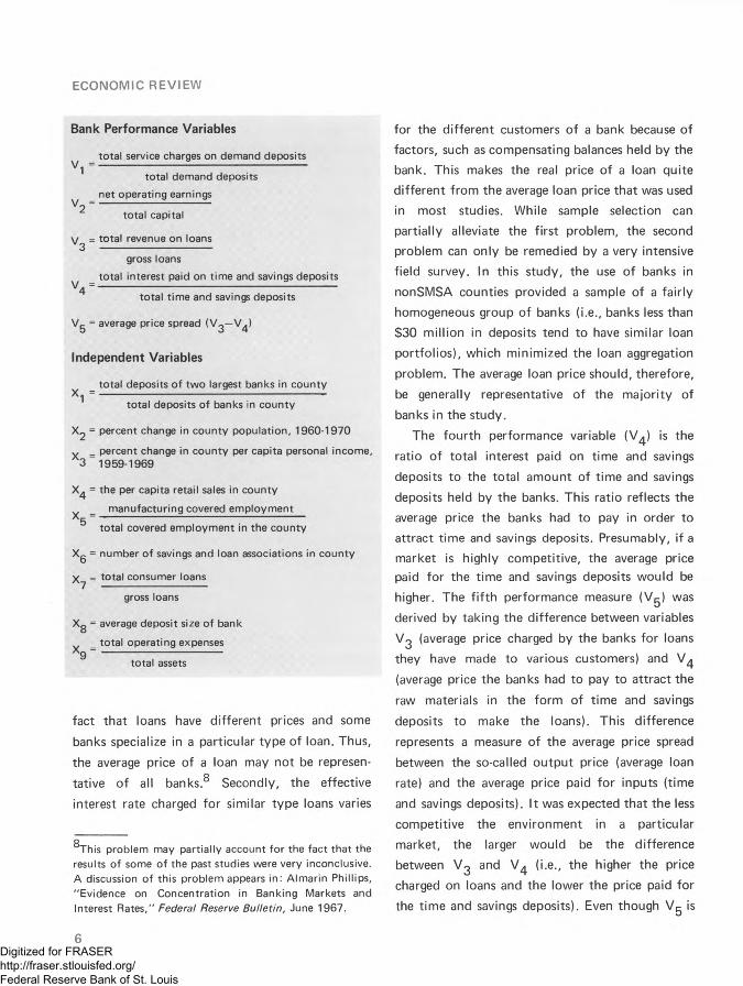
Bank Performance Variables

total service charges on demand depositsV1 =

V2 =

total demand deposits

net operating earnings

total capital

V = total revenue on loans3 ------------------------------------

gross loans

_ total interest paid on time and savings deposits

total tim e and savings deposits

Vj- = average price spread (V ^ —V^)

Independent Variables

total deposits o f two largest banks in countyX1 = total deposits of banks in county

= percent change in county population, 1960-1970

y _ percent change in county per capita personal income, 3 1959-1969

= the per capita retail sales in county

v _ manufacturing covered employment

total covered employment in the county

Xg = number of savings and loan associations in county

y = total consumer loans7 ---------------------------------

gross loans

Xg = average deposit size of bank

total operating expensesX9 =

total assets

fact that loans have d ifferent prices and some

banks specialize in a particular type o f loan. Thus,

the average price o f a loan may not be represen

tative o f all banks.8 Secondly, the effective

interest rate charged fo r similar type loans varies

This problem may partially account for the fact that the results of some of the past studies were very inconclusive. A discussion of this problem appears in: Almarin Phillips, "Evidence on Concentration in Banking Markets andInterest Rates," Federal Reserve B u lle tin , June 1967.

fo r the d ifferent customers o f a bank because o f

factors, such as compensating balances held by the

bank. This makes the real price o f a loan quite

d ifferent from the average loan price that was used

in most studies. While sample selection can

partia lly alleviate the firs t problem, the second

problem can only be remedied by a very intensive

field survey. In this study, the use o f banks in

nonSMSA counties provided a sample o f a fa irly

homogeneous group o f banks (i.e., banks less than

$30 m illion in deposits tend to have similar loan

portfo lios), which minimized the loan aggregation

problem. The average loan price should, therefore,

be generally representative o f the m ajority of

banks in the study.

The fourth performance variable (V^) is the

ratio o f to ta l interest paid on time and savings

deposits to the tota l amount o f time and savings

deposits held by the banks. This ratio reflects the

average price the banks had to pay in order to

attract time and savings deposits. Presumably, if a

market is highly competitive, the average price paid fo r the time and savings deposits would be

higher. The f if th performance measure (Vg) was

derived by taking the difference between variables

Vg (average price charged by the banks fo r loans

they have made to various customers) and V ^

(average price the banks had to pay to attract the

raw materials in the form o f time and savings

deposits to make the loans). This difference

represents a measure o f the average price spread

between the so-called ou tput price (average loan

rate) and the average price paid fo r inputs (time

and savings deposits). I t was expected that the less

competitive the environment in a particular

market, the larger would be the difference

between Vg and V ^ (i.e., the higher the price

charged on loans and the lower the price paid fo r

the time and savings deposits). Even though V ^ is


MARCH 1972

dependent upon Vg and V ^, it does perm it an

observation o f the structure-performance question

in a slightly d ifferent manner.

DETERMINANTS OF BANK PERFORMANCE

The operating performance o f banks was

assumed to be a function o f banking structure as

well as other bank and market variables. In most

structure-performance studies, the structure of a

market was generally proxied by a concentration

ratio, which indicates the percentage of deposits

held by the largest bank or banks in the market.9

In this study, the two-bank concentration ratio, or

the percentage of deposits held by the two largest

banks in the market (X ^), was used to proxy

banking structure. The two-bank ratio was used

because it provided an accurate picture of banking

structure in the nonSMSA county markets that

were used in the study. The assumption was made

that the higher the concentration ratio in any

single market, the less competitive would be the

environment in that market.

Market variables that could affect the perfor

mance o f banks can generally be put in to the

classification of "economic ac tiv ity ” or "demand”

variables. It can be expected that the comparative

performance o f banks in two separate markets

would be affected by the d iffering levels of

economic activ ity, or demand fo r banking services,

even if the banking structure is the same. Four

variables were used in this study as proxies for

economic activ ity in the individual markets: (1)

the percentage change in county population from

gThe number of banks in a market is sometimes used as a

structural proxy. However, both Fraser and Rose and Kaufman found that from a statistical viewpoint the concentration ratio and the number of banks in a market area were equally good proxies for the banking structure.

1960-1970 (X 2 ), (2) the percentage change in

county per capita personal income from 1959 to

1969 (Xg), (3) the per capita retail sales in the

county (X^) fo r 1969 and 1970, and (4) manufac

tu r in g employment covered by the State

unemployment insurance as a percent o f total

covered employment in the county (X^). Variables

X 2 and Xg serve as proxies fo r shifts in demand

for banking services in a market, and X ^ is a proxy

fo r the level of demand. Variable Xg was used to

control fo r differences in the level of industrial

activity among the markets. It was assumed that

the more highly industrialized markets would have

a higher level of economic activ ity.

A sixth market variable was also included to

take account o f existing and potential competition

provided by other financial institutions in each

market. The proxy used fo r this effect was the

number o f savings and loan associations operating

in each market (Xg). Presumably, if a large

number o f savings and loan associations are

operating in a particular market, there would be a

significant amount o f com petition fo r time

deposits and certain types of loans in the

markets.10

Three bank variables were used to take account

of bank operations that could alter bank perfor

mance. One of these variables is the percent of

total loans held in the consumer loan category by

the banks in each market (Xy). Even though the

banks in the sample are fa irly homogeneous, this

variable was intended to help control fo r d iffe r

ences in loan mix that could have an effect upon

10The same values for variables X 2 , X 3 , X 5 , and Xg wereused in both the 1969 and 1970 regression equations. This should not hinder the analysis since these data do not change significantly in one year. The number of savings and loan associations was used in X q because data were not available on the deposits of savings and loan associations by nonSMSA counties.


ECONOMIC REVIEW

the performance variables. Another bank variable,

average bank size (Xg), provided an additional

control fo r d iffering bank behavior among

markets. Larger banks tend to behave d ifferently

w ith respect to loan mix and some prices. The

ratio o f average tota l operating expenses to average

total assets fo r the banks in each market (Xg)

presumably measures, on a market level, how

e ffic ien tly banks are managed.11 Some banks may

be operated more e ffic ien tly than others, which

would have an effect on market performance. In

order to isolate the effect of market structure

upon performance, it is necessary, therefore, to

control fo r the effect that other variables, such as

efficiency, may have on performance.

TECHNIQUES AND RESULTSThe structure-performance relationship among

banks headquartered in the 57 nonSMSA counties

in Ohio was investigated using m ultip le regression

te c h n iq u e . Cross-sectional regressions were

computed fo r two d ifferent years, 1969 and 1970,

to observe the structure-performance relationships

under d ifferent monetary conditions. Data fo r

the banks in the 57 counties were taken from the

December 1969 and December 1970 "Reports of

C ond ition" and "Reports o f Earnings and D ivi

dends," as compiled by bank regulatory agencies.

It was assumed that the performance variable

(V), which is the average of the values o f this

variable fo r all o f the banks in a market, was a

function o f the concentration (X-|) and economic

1 1 Under certain circumstances the bank cost ratio could be viewed as a bank performance variable. However, in this study the cost ratio is only assumed to be a proxy for the differences in bank efficiency that may have an effect on bank performance.

12The year 1969 was a relatively tight money period while 1970 was a period of relative monetary ease.

activity (X 2 —Xg) in the county as well as the

types o f banks operating in the market (X y—Xg).

Therefore,

V jj = F (X^j,...,Xg j) where i = performance measure

and j = market

There are 57 separate markets or observations in

the study. The fo llow ing sections discuss the study

results in detail. The Table summarizes the

empirical findings; the actual statistical results are

presented in the Appendix.

Service Charge or Demand Deposits. Results

from this set o f equations fail to indicate that

bank concentration has an im portant effect on the

average service charge on demand deposits. The

relationship between service charges and concen

tration in the 57 nonSMSA counties is weak, w ith

the degree o f association insignificant (at the 5

percent level) in both 1969 and 1970. On the

other hand, increases in concentration (as

indicated by positive coefficients) may tend to

increase the average service charge, but the size of

this increase would be relatively small.

Bank cost and bank size are significantly related

to service charges on demand deposits. The

variable fo r bank costs is significant (at the 0.1

percent level) in both 1969 and 1970, and the

positive sign on the coefficients indicates that

banks w ith relatively high total operating cost/

asset ratios tend to charge more fo r their demand

deposits. This result may simply im ply that the

less e ffic ien t banks must, and are able to , charge a

13 The estimated change in the average service charge brought about by an increase in the concentration ratio can be computed by taking the concentration coefficient and multiplying it by a representative change in the concentration ratio.


Summary o f Results o f Structure-Performance Tests for NonSMSA Counties in Ohio Independent Variables

Number ofPercent Percent Savings and

Performance Concentration Change in Change in Retail Sales Industrialization Loan Consumer Loans/ Average BankVariables Ratio Population Income Per Capita Ratio Associations Gross Loans Size Cost Ratio

1969X 1 X 2 X 3 X 4 X 5 X 6 X 7 X 8 X 9

V ^—Average service charge on demand deposits

insignificant insignificant insignificant insignificant insignificant insignificant insignificant significantpositive

significantpositive

V j —Profit rate insignificant insignificant insignificant insignificant insignificant insignificant significantpositive

insignificant significantnegative

V g —Average loan rate insignificant insignificant insignificant significantnegative

insignificant significantpositive

insignificant insignificant significantpositive

V ^ —Average savings rate insignificant significantpositive




V ,-—Price spread

1970

insignificant insignificant insignificant significantnegative

insignificant insignificant insignificant insignificant insignificant

V ^—Average service charge on demand deposits

insignificant insignificant insignificant insignificant insignificant insignificant insignificant significantpositive

significantpositive

Profit rate insignificant significantpositive

insignificant insignificant significantnegative


significantpositive

significantnegative

V g —Average loan rate insignificant insignificant significantpositive



significantpositive

V ^—Average savings rate insignificant insignificant significantpositive

significantpositive

insignificant insignificant insignificant significantpositive

significantnegative

V g —Price spread significant insignificant insignificant insignificantpositive

NO TE : Coefficients are significant at the 5 percent critical level. When significant, the sign is indicated.

Source: Federal Reserve Bank of Cleveland



insignificant


ECONOMIC REVIEW

1 4higher price fo r their demand deposits. Bank

size and the average service charges on demand

deposits are also significantly and positively

related fo r both 1969 and 1970. This means that

those banks located in counties w ith a relatively

high average deposit size tended to charge more

fo r their demand deposits than banks in counties

w ith a low average deposit size. This result may

im ply that relatively large banks in the study are

located in less competitive market areas. There

fore, they were able to implement higher service

charges on demand deposits.1 5

The coefficients o f the savings and loan associ

ation variables and the four variables fo r economic

activ ity show no significant relationship to

demand deposit service charges fo r either 1969 or

1970.

Net Operating Earnings to Total Capital. The

performance variable in this analysis measures

p ro fita b ility of a bank related to its total invested

capital. It was hypothesized that banks would be

less profitable in a highly competitive market. This

hypothesis was somewhat confirmed by the test

results, but the findings are relatively insignificant.

For 1969, the concentration variable is significant

at the 20 percent level, but is insignificant fo r

1970. The positive sign on the coefficients,

however, suggests that a high rate o f p ro fit is

positively related to a high concentration ratio.

On the other hand, bank p ro fitab ility is s ignifi

cantly affected by tw o of the three bank

variables—costs and consumer loan/gross lo a n -

according to equations fo r both 1969 and 1970.

14The simple correlation coefficients between bank costs and concentration are —0.18 and —0.14 for 1969 and 1970, respectively.

15This point is substantiated somewhat by positive correlation coefficients between bank size and concentration of 0 .22 and 0.19 for 1969 and 1970, respectively.

The cost ratio is negatively related to the p ro fit

rate, indicating that banks in markets w ith rela

tive ly higher average costs generally have lower

profits. The consumer loan/gross loan variable has

a positive sign, indicating that the banks in the

more profitable markets had a larger percentage of

consumer loans in their po rtfo lio . This result is

consistent w ith other evidence tha t indicates

consumer loans tend to be more profitable fo r

banks than some other types of loans.

There is no significant impact on bank p ro fit

ab ility from the economic activ ity variables fo r

1969. For 1970, however, the population variable

and the industrialization variable are significantly

related to the p ro fit rate.16 The sign on the

population variable is positive, indicating that

banks in markets that had large increases in

population also had high p ro fit rates. The indus

tria lization variable has a coeffic ient w ith a

negative sign, which implies that banks operating

in the more industrialized markets tended to have

lower p ro fit rates. This may reflect the fact that

these banks must compete w ith large c ity banks

for the more profitable commercial and industrial

loans that are available in these markets.

Bank p ro fita b ility in the 57 nonSMSA counties

does not appear to have been affected by compe

titio n from savings and loan institutions.

Average Loan Rate. The conclusion that

emerges from the analysis o f variables that affect

loan rates o f the banks under study is that the

relationship between bank concentration and the

loan rate is weak, while the relationship between

costs, income, and the number o f savings and loan

associations is significant. Specifically, the rela

tionship between concentration and average loan

16This result implies that the economic activity variables become more sensitive with respect to profit rates duringperiods of monetary ease.


MARCH 1972

rates is weak fo r both 1969 and 1970, and the

impact o f an increase in bank concentration

appears relatively small; i.e., an increase in the

concentration ratio o f 20 percentage points would

have only increased the average loan rate in 1970

by approximately 0.1 percent.1 7

The bank cost variable is highly significant fo r

both years, and the positive sign on the coefficient

indicates tha t banks w ith relatively high costs also

charged high average rates on their loans. This

result is similar to the one on average service

charges on demand deposits and suggests that the

less effic ient banks in these markets are able to

charge higher rates fo r their services.

Per capita retail sales and per capita income

were found to be significantly related to higher

loan rates, although fo r d ifferent years. For 1969,

the retail sales per capita variable implies that

counties w ith high retail sales per capita had

relatively lower average loan rates. The level of

retail sales per capita was assumed to proxy the

intensity of economic activ ity in a market; and,

therefore, the lower average loan rate would be

consistent w ith this assumption. For 1970, the per

capita income variable indicates increasing demand

fo r bank services; and, therefore, it would be

directly related to the average loan rates.

Finally, the operation of savings and loan

associations has a significant and positive relation

ship w ith bank loan rates. Results of equations fo r

1969 and 1970 indicate that banks operating in

17The average loan rate may have been more precisely

measured for 1970 than for 1969, which was a tight money period with increasing loan rates. Since there are usury ceilings in Ohio, the 1969 average loan rate may not represent the effective loan rate. In 1970, however, monetary policy was less restrictive, and loan rates tended to be lower. Therefore, the 1970 average loan rate and the effective loan rate would probably be approximately at the same level.

markets that contain a relatively large number of

savings and loan associations had a higher average

loan rate. This may im ply that, because savings

and loan institutions specialize in real estate loans,

banks in markets w ith several such institutions

tend to concentrate on selling other types o f loans,

possibly because the com petition is less intense in

these other areas.18 Since the rates on real estate

loans are generally lower than the rates on

consumer and some other types o f loans, the

tendency o f holding fewer real estate loans in a

po rtfo lio would therefore result in a higher average

loan rate fo r the commercial banks in those

markets. Thus, it appears that in markets where

there are a relatively large number o f saving and

loan associations, banks had a higher average loan

rate.

Average Time and Savings Rate. Bank concen

tration in nonSMSA county markets in Ohio does

not appear to have had an im portant impact on

the average savings rate paid by banks in those

markets. In both the 1969 and 1970 equations,

the relationship between concentration and the

rate paid on deposits is insignificant.

Bank costs, however, are highly significant in

both equations, and the sign on the coefficients

indicates a direct relationship between the average1 Qsavings rate and the cost ratio. This relationship

implies that those banks operating in high average

18This result is supported by the correlation coefficients between the number of savings and loan associations in a market and the percentage of various types of loans held by banks in those markets. There was a negative correlation between the number of savings and loan associations and the percentage of consumer and commercial loans held by banks in these markets.

19 Part of the significance of this relationship is because of the fact that the total operating costs include the interest paid on time and savings deposits.


ECONOMIC REVIEW

cost markets paid a relatively high average savings

rate.

The level of retail sales per capita is also

significant in both the 1969 and 1970 equations.

This result implies that a high level o f per capita

retail sales was associated w ith a high average time

and savings deposit rate. Since retail sales per

capita was viewed as a proxy fo r the level of

economic activ ity in a market, this result is

consistent w ith a high average time and savings

rate.

F inally, there is little relationship between the

number o f savings and loan associations and the

rates paid on time and savings deposits, according

to equations fo r 1969 and 1970. This result is a

little surprising because it could be expected that

savings and loan associations compete d irectly

w ith banks fo r time and savings deposits and

would, therefore, drive up the average savings rate.

However, the relationship could be distorted by

the rate ceilings imposed on both types o f ins titu

tions, which would lim it their com petition w ith

each other.20 This factor could account fo r the

absence o f a relationship between the number of

savings and loan associations and the banks'

average savings rate.

Average Price Spread. The relationship between

the average price spread and concentration is

highly significant in the 1970 equation, but is

insignificant in the 1969 equation. Both equations

show a positive association, im plying that a

relatively large price spread is associated w ith a

high level o f concentration in the 57 banking

20 Savings and loan associations have higher ceiling rates than commercial banks. The Federal Reserve System, however, lifted some of the rate ceilings in 1970 for large denomination time deposits. This change would probably not have a great effect on the present findings since many of the banks in this sample do not offer that type of time deposit.

markets. However, the relationship is relatively

weak, as evidenced by the fact tha t a 20

percentage po in t increase in the two-bank concen

tration ratio would have only increased the average

price spread by approximately .002 percent in

1970.

The wide difference in the relationship between

the price spread and concentration fo r 1969 and

1970 is most like ly a result o f the type of

monetary policy that was being pursued in both

years. In 1969, policy was restrictive and loan

rates and deposit rates were relatively high.

However, usury laws in Ohio kept some loans rates

from increasing to their natural level, and Regu

lation Q prohibited the deposit rates fo r increasing

beyond their stated ceilings, causing the spread

between the rates to be distorted. In 1970, as the

supply o f credit expanded, both loan rates and

savings rates fell somewhat from their ceiling

levels. The demand and supply forces operating in

the market, therefore, were relatively free to

produce a price spread that was essentially undis

torted. As a result, it can be expected that the

relationship between concentration and the

average price spread is measured more accurately

fo r 1970 than fo r 1969.

The number o f savings and loan associations in

the banking markets under study was found to

exert some influence on price spread. The positive

sign on the savings and loan variable indicates that

a relatively large number o f these institu tions in a

market is associated w ith a large price spread fo r

the banks in those markets. This is consistent w ith

the earlier findings on the average loan rate and

average savings rate equations. It could be hypoth

esized that savings and loan associations do not

offer commercial banks as much direct compe

tition fo r financial services as m ight be expected.

In fact, the presence o f a relatively large number


MARCH 1972

of savings and loan associations in a market may

provide banks w ith an incentive to concentrate on

providing financial services that are not offered by

savings and loan associations.

The relationship between price spread and

other variables examined—such as per capita retail

sales—is generally insignificant. The retail sales per

capita variable is significant in the 1969 equation,

but insignificant fo r 1970. The negative relation

ship between retail sales per capita and the price

spread is consistent w ith earlier results.

SUMMARY AND CONCLUSIONSThis study generally concludes that the

structure o f markets (as represented by a two-bank

concentration ratio) is not strongly related to the

aggregate performance o f banks in the nonSMSA

markets in Ohio. The study differs somewhat from

other such studies in that it was lim ited specif

ically to nonSMSA county markets in order to

obtain a more homogenous sample fo r the

empirical tests.

The only specific variable that appeared to have

had a consistent impact on bank performance is

the bank cost ratio. This variable is significant in

three o f the four equations fo r both 1969 and

1970, implying that bank efficiency may be an

im portant determinant of the performance of

banks in the nonSMSA county markets. There

may be at least tw o reasons why most studies of

this type have not consistently shown a strong

relationship between market structure and bank

performance. First, banking is a regulated

industry. Many o f the regulations tend to diminish

the significance o f the relationship between

structure and bank performance since the market

is not entirely free to determine prices and output

and to reward the e ffic ient or punish the

ineffic ient performer.21

Secondly, the results from this study may

imply that the approach used to measure bank

performance was not suffic iently disaggregated to

isolate the structure-performance relationship as it

exists fo r banks in these nonSMSA county

markets. While the structure of a market affects

some aspects o f bank performance, it may be very

d iff ic u lt to detect the extent o f the relationship

w ith aggregate performance variables. Additional

research using disaggregated variables of bank

performance (mortgage loan rates or business loan

rates instead of average loan rates) is necessary to

measure precisely how great an impact marketo o

structure has on bank performance. This type of

research must be completed fo r individual states

and fo r d ifferent markets w ith in states before any

generalized statements can be made w ith regard to

the b a n k in g industry and the structure-

performance relationship.

21 For a discussion of this point see: Almarin Phillips, "Com petition, Confusion, and Commercial Banking," The Journa l o f Finance, March 1964.

22 For example see: Donald Jacobs, Business Loan Costs and Bank M arke t S truc tu re (New York: National Bureau of Economic Research, 1971).


APPENDIX TABLE

Statistical Results of Structure-Performance Relationship Tests for NonSMSA Counties in Ohio

PerformanceVariables Intercept

ConcentrationRatio

Percent Change in Population

Percent Change in

Income

1969 X1 x2 X3V j— Average service charge

on demand deposits-.29112 X 10~2 .94213 X 10- 3

(.78239).26268 X 10- 4

(.81942)-.56828 X 10-6

(-.70743)

V2— Profit rate .13929 .36004 X 10-1 (1.49472)

.34542 X 10~3 (.53865)

-.33158 X 10 -5 (-.20634)

V^—Average loan rate .44813 X 10—1 .66914 X 10~3 (.22360)

.11717 X 10~3 (1.47080)

.46376 X 10~6 (.23230)

V^—Average savings rate .16587 X 10-1 .22414 X 10- 3 (.97930 X 10~1)

.12226 X 10- 3 * (2.00654)

.14487 X 10~5 (.94884)

Vg—Price spread .28226 X 1CT1 .44500 X 10- 3 (.14438)

-.50878 X 10~5 (-.62007 X 10~1

.98500 X 10-6 ) (-.47906)

1970

V^—Average service charge on demand deposits

-.24666 X 10- 2 .91616 X 10- 3 (.70129)

.39042 X 10~4 (1.15806)

-.27094 X 10-6 (-.30953)

V j—Profit rate .27117 .26421 X 10~1 (1.16675)

.11794 X 10- 2 * (2.01821)

.15707 X 10~5 (.10351)

Vg—Average loan rate .42282 X 10-1 .56482 X 10- 2 (1.48064)

.11218 X 10- 3 (1.13958)

.45742 X 10"5* (1.78961)

V4~Average savings rate .24809 X 10“ 1 -.29472 X 10~2 (-1.24553)

.66502 X 10~4 (1.08903)

.35315 X 10~5* (2.22741)

Vg—Price spread .17472 X 10~1 .85955 X 10~2* (2.41178)

.45683 X 10-4 (.49670)

.10427 X 10-5 (.43664)

NOTE: Figures in parentheses are t-values.

* Significant at the 5 percent level, t Significant at the 1 percent level.

Source: Federal Reserve Bank of Cleveland

Retail Sales Per Capita

IndustrializationRatio

Number of Savings and

Loan Associations

Consumer Loans/ Gross Loans

Average Bank Size Cost Ratio R2

X4 X5 X6 X7 X8 X9.73054 X 10- 3

(-1.14822).29635 X 10~5

(.19977).16071 X 10- 3

(1.18134).28650 X 10- 3

(.13477).66004 X 10- 7 *

(2.11502).17510t

(3.61064)51.4

.15612 X 10~1 (1.22672)

-.60545 X 10- 4 (-.20590)

.18304 X 10- 2 (.67260)

.93011 X 10_ 1 * (2.18729)

-.47945 X 10-6 (-.76802)

—1.72600* (-1.77914)

26.1

-.28203 X 10- 2 * (-1.78375)

.14805 X 10-4 (.40529)

.58994 X 10_3# (1.74493) I

-.1 3 8 4 9 X 1 0 3 -.3 259 2X 10 8 [-.26216 X 10—1) (-.42024 X 10- 1 )

.48180t (3.99762)

43.2

.20935 X 10_2# (1.73115)

-.35645 X 10- 4 (-1.27582)

-.71634 X 10- 4 (-.27703)

-.88715X 10 2* (2.19566)

-.19796 X 10 7 (-.33373)

.50038t(5.42831)

60.6

-.49138 X 10_ 2 t (-3.01747)

.50450 X 10-4 (1.34095)

.66157 X 10- 3 (1.34095)

.87330 X 10- 2 (1.60506)

.16536 X 10~7 (.20702)

-.18575 X 10“ (-.14964)

1 32.8

-.69165 X 10- 3 (-1.37266)

.53850 X 10- 6 (.33964 X 10~1)

.23438 X 10- 3 (1.54791)

-.54663 X 10- 3 (-.21476)

.61106 X IQ '7* (2.05432)

.15238t (3.33138)

48.6

-.31025 X 10- 2 - (-.35520)

-.55160 X 10- 3 * (-2.00705)

.20936 X 10~2 (.79767)

.11881 + (2.69298)

.28658 X 10- 6 (.55581)

—3.64484t (-4.59683)

44.7

-.19429 X 10- 3 (-.13205)

-.49444 X 10—4 (-1.06799)

.100088 X 10_2# (2.28170)

.56415 X 10- 2 (.75906)

.56205 X 10- 8 (.64710 X 10 1)

.43478t(3.25515)

41.8

.17197 X 10- 2 * (1.88431)

-.23025 X 10~4 (-.80178)

-.20095 X 10- 3 (-.73270)

-.40452 X 10- 2 (-.87745)

.34851 X 10” 7 (.64686)

.33504t(4.04385)

49.2

-.19140 X 10“ 2 (-1.39242)

-.26418 X 10- 4 (-.61078)

.12097 X 10- 2 t (2.92872)

.96868 X 10- 2 (1.39505)

-.29231 X 10-7 (-.36021)

.99741 X 10-1 (.79929)

35.8


MARCH 1972

THE STRUCTURE OF STATE REVENUE

INTRODUCTIONState governments have been faced w ith both

increased operational costs and continually

growing demands fo r public services. As a result,

the states have found it necessary to increase tax

rates and institute new taxes. They have also

turned to the Federal Government fo r financial

aid. In the past. Federal aid has been in the form

of grants fo r specific programs; but in the future,

some funds may be distributed through a form o f

revenue sharing fo r use largely at the discretion o f the recipient government. The proposals fo r

revenue sharing that are currently being considered

are based on factors such as population, per capita

income, and tax e ffo rt o f the individual govern

ment unit.

This article discusses the variation in state tax

structure and tax e ffo rt and d ifferent aspects o f

the principal taxes now used by the states,

particularly those states in the Fourth D istrict.

The possible impacts o f a revenue sharing program

and state funding o f local schools on the state

revenue structures are also examined. The dis

cussion and data relate only to taxation at the

state level (thus excluding taxes imposed by cities,

counties, and school districts) and do not account

fo r differences in services provided at the state

Warren E. Farb

level. (Services provided at the state government

level in some states may be provided by counties

or municipalities in other states.)1

TAX STRUCTUREThe amount o f revenue that a taxing authority

is able to raise is necessarily lim ited by the size of

the relevant tax bases. The principal bases are

income, sales, and wealth (property tax), although

other measurable concepts could be used. A range

in possible rates as well as numerous combinations

of taxes leads to greatly d iffering tax structures

and, consequently, variations in tax e ffo rt among

the states. The d iffe ren t tax structures make it

v irtua lly impossible to develop a clear-cut measure

of e ffo rt. For example, one state may be making a

strong e ffo rt in terms o f the wealth base, but its

e ffo rt may appear weak when compared to the

income base.

The measure o f tax e ffo rt discussed in this

article is revenue per $1,000 o f personal income,

which tends to remove the effects o f differences in

income levels among states stemming from either

1For a more complete study, see: "State and Local

Revenues and Expenditures," E conom ic Review, Federal Reserve Bank of Cleveland, November 1970.


ECONOMIC REVIEW

TABLE I

Rank o f States' Revenue Per $1,000 o f Personal Income*Selected Revenue Sources1970

Per Capita Personal Income

Total Tax Revenue

General Sales or Gross Receipts

Individual Income Tax

1 Connecticut $4 ,595 Hawaii $111.26 Hawaii $53.17 Hawaii $34.322 Alaska 4,460 New Mexico 94.99 Mississippi 43 .55 Wisconsin 31.863 Nevada 4,458 Verm ont 94 .80 Washington 41.72 Delaware 30.884 New York 4,442 Mississippi 92.81 West Virginia 38.38 New York 30.805 California 4 ,290 Delaware 8 8 . 2 1 Arizona 30.43 Vermont 30.62

46 South Carolina 2,607 Missouri 51 .03 New York 12.44 Louisiana 4.6147 West Virginia 2,603 Nebraska 49 .96 Oklahoma 11.99 New Hampshire 1.3948 Alabama 2,582 New Jersey 43.95 Verm ont 11.97 Tennessee 1.0849 Arkansas 2,488 Ohio 42.41 New Jersey 11.73 New Jersey 0.5850 Mississippi 2,218 New Hampshire 38.07 Massachusetts 7.41 Connecticut 0.36

* Personal income data are U. S. Department o f Commerce estimates for calendar year 1969.

Source: U. S. Department of Commerce

d iffe ren t populations or levels o f per capita

income.2 Although this measure ignores "w ea lth "

and levels o f economic activ ity, most states

recognize income as the major source of tax revenue.

Tax e ffo rt—as measured by revenue per $1,000

of personal income—varies greatly among the

states because o f variations in income or d iffe r

ences in tax structure (see Table I). The average

state tax was $67 per $1,000 of personal

income in 1970, and ranged from $38 in New

Hampshire to $111 in Hawaii. O f the five states

that ranked highest in per capita personal income

in 1970, none was among the top five in tax

e ffo rt; on the other hand, o f the lowest ranked

states in per capita income, one state (Mississippi)

ranked among the top five in revenues collected.

In general, tax e ffo rt and per capita income show ao

Tax effort measured by tax per $1 ,000 of income is a widely used definition, but it does have many shortcomings and is by no means the only measure of tax effort found in economic literature. For a more detailed discussion of measures o f tax effort and tax capacity see: Allen D. Manvel, “ Differences in Fiscal Capacity and E ffort: Their Significance for a Federal Revenue Sharing System," N ation a l Tax Journa l, Vol. X X IV , No. 2 (1971).

weak negative correlation, suggesting that states

w ith relatively high per capita incomes do not

necessarily have the lowest tax efforts. Of the five

states w ith the highest revenue per $1,000 o f

personal income, all but New Mexico are among

the five top states in either income or sales tax

efforts. S im ilarly, those states having the lowest

overall tax e ffo rt either do not use one o f the two

major types o f state taxation or use them to only a

lim ited extent. Ohio, which did not have a state

income tax in 1970, and New Hampshire, which

does not have a sales tax, are examples o f the

former, and New Jersey is an example o f theo

latter. The sources and relative d istribution o f tax

revenue fo r the five states that rank as the highest

in overall tax e ffo rt and the five states that rank

the lowest are shown in Table II. Tables I and II

both illustrate the large disparity in revenues raised

per $1,000 o f income between the five top ranked

states and the five lowest ranked states. On

average, revenues raised by the five leading states

3Pennsylvania instituted a state income tax in 1971; and

Ohio began levying an income tax in 1972.


MARCH 1972

TABLE II

Percent D istribution o f State Tax Revenue1970

General SalesNationalRank*

Individual I ncome Tax

and Gross Receipts Tax

Corporation Income Tax

AllO thert

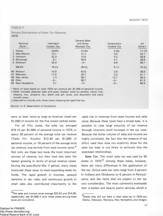
1 Hawaii 30.9% 47.8% 4.3% 17.1%2 New Mexico 13.1 31.3 3.0 52.73 Vermont 32.3 1 2 . 6 4.3 50.84 Mississippi 9.1 46.9 4.1 39.95 Delaware 35.0 - 0 - 6.9 58.1

M EAN 19.2$ 29 .5$ 9 .1 $ 42 .2$

46 Missouri 15.8 42.0 2 . 6 39.647 Nebraska 17.0 28.7 3.3 51.148 New Jersey 1.3 26.7 12.7 59.349 Ohio - 0 - 38.7 - 0 - 61.350 New Hampshire 3.7 - 0 - - 0 - 96.4

* Rank of state based on total 1970 tax revenue per $1 ,000 of personal income, t Other includes selective sales and gross receipts taxes on alcohol, motor fuel,

tobacco, etc., property tax, death and gift taxes, and document and stock transfer taxes.

| Adjusted to include only those states imposing the specified tax.


were at least tw ice as large as revenues raised per

$1,000 o f income fo r the five lowest ranked states.

For all f i f ty states, the sales tax averaged

$19.12 per $1,000 o f personal income in 1970, or

about 30 percent o f the average total tax revenue

(Table III). Another $12.40 per $1,000 o f

personal income, or 19 percent o f the average total

tax revenue, was derived from state income taxes.4

Not only are these tw o taxes the most im portant

sources o f revenue, but they have also been the

fastest growing in terms o f actual revenue raised.

During the post-World War II period, many states

instituted these taxes to meet expanding needs fo r

funds. The rapid growth in incomes, upward

revisions in tax rates, and continuous growth in

retail sales also contributed im portantly to the

4 The sales and income taxes average $22.63 and $14.69 , respectively, per $ 1 , 0 0 0 if only those states levying these taxes are considered.

rapid rise in revenues from state income and sales

taxes. Because these taxes have a broad base, it is

possible to raise large amounts o f tax revenue

through relatively small increases in the tax rates.

Because the dollar volume o f sales and income are

highly correlated, the fact that the measure o f tax

e ffo rt used here does not exp lic itly allow fo r the

sales tax base is not like ly to seriously bias the

expressed relationships.

Sales Tax. The retail sales tax was used by 45

states in 1970.5 Among these states, however,

there are many differences in the application o f

the tax. Actual sales tax rates range from 2 percent

in Indiana and Oklahoma to 6 percent in Pennsyl

vania, and the items that are subject to the tax

vary considerably. The most commonly exempted

item is barber and beauty parlor services, which is

5States that did not have a retail sales tax in 1970 are:

Alaska, Delaware, Montana, New Hampshire, and Oregon.


ECONOMIC REVIEW

TABLE III

Sources and D istribution o f Revenue Per $1,000 o f Personal Income*Average, A ll States 1Q70

Per $1 ,000 Percent of Percent ofSource of Income Total Revenue Total Tax Revenue

Total general revenue Intergovernmental revenue

$104.95 1 0 0 .0 %

from Federal government 25.99 24.8Total tax revenue 64.73 61.7 1 0 0 .0 %

General sales tax 19.12 29.5Individual income tax 12.40 19.2Other taxest 33.21 51.3

Other revenue^ 14.23 13.5

* Personal income data are U. S. Department of Commerce estimates for calendar year 1969.

tO ther taxes include "other" as defined in Table II plus comparable income taxes and property taxes.

t Consists of revenue received from local governments in the form of shared revenues and grants-in-aid, as reimbursed for services, or in lieu of taxes.


taxed by only seven states. U tilities, especially

local transportation, are also exempted from the

retail sales tax by many states. Other exemptions

range from food and clothing to repair services.

In addition to exempting entire classes o f goods

from general sales taxation, some states allow

special taxes and tax rates on specific items. For

example, Connecticut and some other states

exempt admission charges from the general sales

tax, but impose a separate admission tax. Twenty-

five states allow county and municipal govern

ments to impose a sales tax levy in addition to the

state sales tax. In most states, the additional tax

rate is lim ited to either 0.5 or 1 percent; however,

Alaska allows municipalities to tax at a rate up to

5 percent, and Colorado and New York allow up

to 3 percent.

Regardless o f its form, however, the sales tax is

relatively simple to understand and administer. It

can also be used to obtain large amounts of

revenues, is relatively easy to increase if the need 0

For a complete list of exemptions by state see, State and Loca l Sales Taxes, (New York: Tax Foundation, Inc., 1970).

arises, and is adaptable to sharing w ith other

government units.7

Income Tax. A state personal income tax is

more complicated to administer than the sales tax,

but most states that use the income tax try to keep it as simple as possible. In comparison w ith

the Federal income tax, these efforts have been

successful.

O f the 44 states that used a personal income

tax in 1970, Verm ont and Alaska opted fo r the

simplest o f all methods—a fixed percentage tax

levy on individual Federal income tax liab ility . For

the other states, complications are introduced at

two levels: (1) in calculating the tax base and (2)

in determining the applicable tax rate.

In some states, the defin ition o f income fo r tax

purposes is related to one o f the several income

concepts used in the Federal income tax return,

while in other states the tax base is independent of

the Federal income tax. States may or may not

a llow standard or itemized deductions or

7Of the 25 states that permit a local sales tax levy in addition to the state sales tax, 19 administer the entire tax at the state level.


MARCH 1972

deductions fo r Federal taxes. A ll states provide fo r some type o f personal exemption, but both the

size and the rules governing the exemption vary

w idely. For example, Maryland allows $800 per

person; Mississippi allows $4,000 fo r a single

individual and $6,000 fo r a fam ily; and Wisconsin

allows a tax credit o f $10 per person to be applied

to the actual tax bill.

The rate structures o f the state personal income

taxes can be classified into two general categories:

graduated and fla t. By far the most popular

method is the graduated rate structure, and it is

used by over two-thirds o f the income taxing

states. The New York income tax structure begins

w ith a 2 percent rate on the first $1,000 o f income

and increases to 14 percent on income over

$23,000. The fla t rate tax generally tends to be a

relatively low rate, such as the 2 percent used in

Indiana. Another form o f the fla t rate tax is a

fixed percentage o f Federal income tax liab ility ,

which is used by Alaska and Vermont. This

method, although a fla t rate, tends to tax high

incomes more heavily than low incomes because o f

the graduated rates bu ilt into the Federal tax

structure.

When the fla t rate income tax is used, revenue

can be increased in a manner similar to retail sales

tax; all that is required is the enactment of

appropriate legislation. With a graduated tax,

however, new schedules must be constructed.

Depending on the priorities o f the state, the

increase can be evenly spread out over all incomes

or concentrated on one or more income levels.

With an income tax, it is also possible to change

the amount o f total revenue raised by the tax

w ithou t changing the tax rate structures. This can

be accomplished by changing the rules concerning

exemptions, deductions, and credits or by altering

the defin ition o f taxable income.

The graduated income tax is generally regarded

to be the most progressive o f the major sources o fO

state tax revenue w ith respect to income. An

income tax based on a fla t rate generally is

considered to be proportional; and a sales tax,

regressive. However, the various adjustments and

alternatives to the tax base that are permitted

under the state laws have drastically altered these

general relationships. The fla t rate personal

exemption, fo r instance, which is used in many

graduated income taxes, tends to lessen the degree

o f progressiveness because an individual in a high

tax bracket w ill benefit more from the exemption

than an individual in a lower tax bracket. With

respect to the retail sales tax, exemptions can

make the tax less regressive. Therefore, the low

income individual would receive the greatest

benefit from the exemption o f a necessity such as

food from the sales tax base, causing a lower

degree o f regressiveness.

Intergovernmental Transfers. Another major

source of revenue fo r state governments, which has

been increasing rapidly in recent years, is inter

governmental transfers from the Federal Govern

ment. Most o f the funds are currently earmarked

fo r specific uses, such as highway construction,

education, and welfare. However, there has been

considerable debate concerning the desirability o f

allowing the recipient, both governments and

individuals, fu ll discretion in spending transferred

funds. Under most "revenue sharing" plans, the

ONo other single source of tax revenue contributes as

much as 1 0 percent of total revenue, and only the corporate income tax contributes as much as 5 percent (see Table II) . In this article, a tax is considered to be progressive if the amount of tax paid as a percentage of income increases as income increases. If the percentage of income paid as tax is equal for all income levels, the tax is considered to be proportional; and if the percentage decreases, the tax is considered regressive.


ECONOMIC REVIEW

recipient government un it would be granted a

specified share o f designated funds instead o f

receiving fixed amounts o f money fo r a specific

project. One o f the prime objectives o f such plans

is to transfer Federal tax revenue from those areas

o f the country w ith the least pressing need to areas

w ith the greatest relative need. The revenue

sharing plans under consideration in Congress

would make the size o f the grant dependent upon

a complicated formula based on the population,

income level, and possibly the tax e ffo rt o f the

recipient government. In the version recently

approved by the House Ways and Means

Committee, an additional allowance is made fo r

the degree o f urbanization, w ith large urban areas

eligible to receive the greatest benefits.9

In 1970, Federal transfers provided nearly 25

percent o f to ta l state revenue and 40 percent o f

total tax revenue. Nationally, these transfers repre

sented an average o f $25.99 per $1,000 o f

personal income. The range o f Federal transfers,

however, was from $82.24 in Alaska to $15.13 in

New Jersey. In Alaska, only 8.7 percent o f the

general revenue came from the Federal Govern

ment, even though the transfers were 120 percent

o f to ta l tax revenue.10 In New Jersey, even

though the transfers per $1,000 o f income appear

to be small, the Federal payments provided 21.7

percent o f the State's general revenue from all

sources and 34 percent o f its tax revenue.

gThe $5 .3 billion revenue sharing plan agreed to by the

House Ways and Means Committee contains both general and special revenue features. The proposal contains no restrictions on the $ 1 . 8 billion allocated to state governments, while $3 .5 billion allocated to local government units would be restricted to certain types of spending, including capital outlays, maintenance, and operations.

10This is caused by the large amount of general revenuederived through state oil and gas holdings and leases.

In view o f the current debate involving the

relationship o f Federal revenue sharing to state tax

efforts, tax e ffo rt and Federal transfers to states

were statistically related by simple regression

analysis. Results indicate that 21 percent o f the

Federal transfer payments per $1,000 o f personal

income in 1970 were distributed as if they

depended on the tax efforts o f the states

(measured by the tax paid per $1,000 o f personal

income). If the population o f the state were added

to the regression, an additional 10 percent o f the

Federal transfer can be explained. Per capita

transfer payments to states were not as strongly

related to tax e ffo rt and population as were

transfers per $1,000 o f personal income, although

tax e ffo rt did account fo r 12 percent o f the

Federal transfers per capita and population an

additional 4 percent. In general, then, w ithou t

revenue sharing and a specifc formula fo r the

d istribution o f Federal funds, a state's own tax

e ffo rt and population were in fact related to the

state's revenue per $1,000 o f personal income

from the Federal Government in 1970. To date,

revenue sharing proposals have contained formulas

that would take in to consideration a state's

population, some aspects o f its tax e ffo rt, and its

level o f personal income in determining the alio-1 1cation o f funds. It should be noted, however,

that revenue sharing would not replace all o f the

current Federal revenue transfers to states.

Property Tax. In 1970, property tax accounted

fo r only 2.3 percent o f state tax revenue, but 84.9

percent o f local tax revenue. This tax is relatively

unim portant at the state level, but i t does provide

11 It is likely that, if only those funds that are transferred to states at the discretion of the Federal Government—not depending on matching funds or other fixed programs— are studied, the importance of the level of income in the state would increase.


MARCH 1972

the major portion o f local educational funds. Recent rulings by the California Supreme Court

and other state supreme courts, however, have

raised the question o f whether or not the property

tax can be considered an equitable source o f funds

for com m unity schools.12 If the "Californ ia

decision" is upheld, the financing o f public educa

tion could become a state function. If this should

occur, the states would be required to increase

their tax revenue, on average, as much as 80

percent, ceteris paribus. An increase o f such large

proportion in state tax revenue could be financed

through a broad-based tax such as the income or

sales tax. A lthough the additional state taxation

could be offset by lower local property taxes, it is

unlikely that individuals would find the changes

offsetting. Many would find their total state and

local tax burden increased, while others would

find their burden decreased. A lternatively, a

state may decide to maintain the current property

tax structure and to make the state the recipient

rather than the local school district. Either method

would require a greatly expanded revenue e ffo rt

by the state, but would perm it equal d istribution

o f funds among all schools in the state, thus

elim inating the objections raised by the California

court.

TAX STRUCTURE AND FEDERAL TRANSFERS IN THE FOURTH FEDERAL RESERVE DISTRICT

Of the four states included w holly or partly

w ith in the Fourth Federal Reserve D istric t—Ohio, 1~2

Several other state courts, including those in Texas, Minnesota, and New Jersey, have also ruled that the property tax can no longer be used as the primary source of school financing.

13 Alternatively, the Federal Government may provide the needed financing required for education either through general revenue sharing or earmarked grants.

Pennsylvania, Kentucky, and West V irginia—only

Kentucky and West Virginia had both a personal

income tax and a retail sales tax in 1970.14 Ohio

and Pennsylvania rely prim arily on a sales tax,

although Pennsylvania does receive substantial

income from its corporate income tax (see Table

IV). It is, therefore, not surprising that Ohio and

Pennsylvania receive considerably lower tax

revenue per $1,000 o f personal income than

Kentucky and West Virginia. As might be expected

from the previous discussion, Kentucky and West

Virginia, which ranked 43rd and 47th, respec

tively, in per capita personal income among the 50

states—received more intergovernmental transfers

per $1,000 o f personal income (and per capita)

from the Federal Government than Ohio and

Pennsylvania, which ranked 15th and 16th, respec

tively, in per capita personal income. This

d istribution pattern o f Federal transfer payments

possibly reflects the greater need in the relatively

low income states. This is especially true o f West

Virginia, which received more than double the

national average transfer per $1,000 o f personal

income.

The 1970 d istribution o f Federal transfers to

Fourth D istrict states can be compared w ith the

d istribution that would result from any o f the

proposed revenue sharing plans by calculating the

share o f all intergovernmental transfers from the

Federal Government that is allocated to each of

the Fourth D istrict states. The most notable

difference between the 1970 d istribution pattern

and the revenue sharing plan proposed by the

Adm inistration in 1971 is that the two most

populated states in the D istrict (Pennsylvania and

Ohio) would receive a greater proportion o f total

14 Exactly how the tax burden will shift among individuals depends on what taxes are used, what tax schedules are used, and on how the property tax is administered.


TABLE IV

Sources and Distribution of Tax Revenue in the Fourth District States Per $1,000 of Personal Income*1970 Ohio Pennsylvania

Tax Percent of Tax Percent ofper Total Tax National per Total Tax Nation;

$1 ,000 Revenue Rank $1,000 Revenue Rank

Total tax revenue $42.41 100.0% 49 $64.32 100.0% 30

Sales tax 16.41 38.7 34 21.96 34.1 21Individual income tax n.a. n.a. n.a. n.a. n.a. n.a.

Corporation income tax n.a. n.a. n.a. 12.27 19.1 n.a.

Revenue from FederalOther taxest 26 .00 61 .3 n.a. 30.09 46.8 n.a.

Revenue from Federal21.81: 42Government 16.38 23 .5$ 48 20.45

Per capita personal income $3 ,738 15 $3,659 16

n.a. Not applicable.* Personal income data are U. S. Department of Commerce estimates for calendar

year 1969. t As defined in Table II.| As percent of total general revenue.


Kentucky

Tax Percent ofper Total Tax National

$1 ,000 Revenue Rank

$76.40 100.0% 1529.09 38.1 813.20 17.3 19

4.29 5.6 n.a.

29.82 39.0 n.a.

36.66 28.8$ 17

West Virginia

Tax per

$1 ,000

Percent of Total Tax Revenue

NationalRank

$81.31 100.0% 838.38 47.2 4

8.46 10.4 310.82 1.0 n.a.

33.65 41.4 n.a.

53.71 35 .8$ 4

$2,847 43 $2 ,603 47


MARCH 1972

Federal funds, while the other tw o states (West

Virginia and Kentucky) would receive a smaller

proportion o f funds (see Table IV). It is like ly,

however, that the programs that are most sensitive

to need and low levels o f income would continue

independently o f any revenue sharing plan,

although the House Ways and Means Committee

proposal favors those areas w ith the greatest need,

particularly cities and areas w ith low average

incomes.

In the Fourth D istrict, as would be expected,

the tw o states w ith the largest income bases—Ohio

and Pennsylvania—are also the most capable of

increasing their tax revenue. Neither o f these states

had a personal income tax in 1970, although

Pennsylvania did receive 19 percent o f its tax

revenue from a corporate income tax. The revenue

per $1,000 o f personal income received from sales

taxes in these states is also relatively low;

this is probably because o f the exemption o f food

and numerous other items. West Virginia and

Kentucky, however, already rank among the top

15 states in terms o f tax e ffo rt and use both a sales

and in co m e ta x , as well as a c o rp o ra te in com e

tax. In spite o f a relatively low retail sales tax rate

o f 3 percent, West Virginia ranks fourth among all

states in revenue per $1,000 o f personal income

from a sales tax because o f its low level o f per

capita income. The regressions discussed in the

previous section, however, indicate that fo r all 50

states the relation between per capita income and

tax e ffo rt is weak.

SUMMARY AND CONCLUSIONSNearly one-half o f all the 1970 tax revenue at

the state level o f Government was raised through

two broad-based taxes—the personal income tax

and the retail sales tax. The implementation o f

these taxes and the resultant tax e ffo rt vary

greatly among the states. Many o f the state income

taxes have graduated rate structures allowing

progressiveness, but often the degree o f progres

siveness is lessened by income exemptions, deductions, and credits.

Being broad-based, the sales and income taxes

are capable o f raising large amounts o f revenue.

Small increases in the tax rates result in large

increases in tax revenue. Although the property

tax is also broad-based, other things being equal,

its base can be increased only through property

revaluation, and actual rate increases usually

require voter approval. If recent state court

decisions are upheld in higher courts, it is possible

that the financing o f education—which is currently

financed prim arily through property taxation—

may become a state function requiring an increase,

on average, of as much as 80 percent in state tax

revenue.

Another major source o f state revenue that has

been growing in importance is transfers and grants

from the Federal Government. In coming years,

intergovernmental transfers are like ly to increase,

although the method o f d istribution may become

more formalized w ith the advent o f a revenue

sharing or similar program. Congressional pro

posals c u r r e n t l y under consideration fo r

distributing Federal funds to the states include

provisions that take in to consideration not only a

state's population, but also its income level and

possibly its tax e ffort.


rev frbclev 197203

Documents