review of statistical aspects of capital asset …. submission 56... · review of statistical...

Review of Statistical Aspects of Capital

Asset Pricing Model

February 2016

Project: DBP/1

DATA ANALYSIS AUSTRALIA PTY LTD

Review of Statistical Aspects of Capital Asset Pricing Model

February 2016

Client: DBP

Project: DBP/1

Consultants: Dr John Henstridge Dr Kathy Haskard

Anna Munday Jennifer Bramwell

Data Analysis Australia Pty Ltd 97 Broadway

Nedlands, Western Australia 6009 (PO Box 3258 Broadway, Nedlands 6009)

Website: www.daa.com.au Phone: (08) 9468 2533 or (08) 9386 3304

Facsimile: (08) 9386 3202 Email: [email protected]

A.C.N. 009 304 956 A.B.N. 68 009 304 956


DBP/1 ~ Page 1 ~ February 2016 (Ref: Q:\job\dbp1\reports\dbp1_audit_report_20160224.docx)

Table of Contents Expert Opinion – Dr John Henstridge ............... ........................................... 1

Qualifications and Experience ..................... .............................................. 1

Materials Provided ................................ ...................................................... 2

Context ........................................... .............................................................. 3

Structure of This Report ........................................................................... 4

Statistical Background ............................ ...................................................... 5

Linear Models and Prediction .................................................................. 5

Estimation and Regression ...................................................................... 7

Model Adequacy ....................................................................................... 8

Models in the Submission .......................... ................................................. 11

Evaluation Framework Using Portfolios ............................................... 16

Implementation ....................................................................................... 17

Model Adequacy Tests in the Submission ............ .................................... 20

Additional Models ................................................................................... 21

Comparison of Models ........................................................................... 25

Review of the Draft Decision....................... ................................................ 29

Conclusions ....................................... .......................................................... 33

Appendix A – Project Briefing Notes

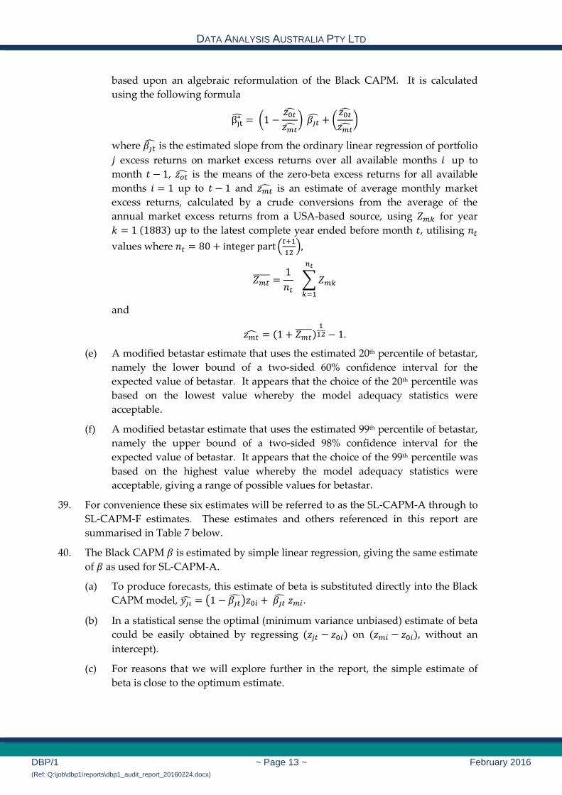
Appendix B – Brief for Extension of Scope

Appendix C – Curriculum Vitae of Dr John Henstridge

Appendix D – Guidelines for Expert Witnesses in Pro ceedings in the Federal Court of Australia



Expert Opinion – Dr John Henstridge 1. I have been asked by DBP to provide an expert statistical opinion on matters related

to the Model Adequacy Test performed as part of their Proposed Revisions DBNGP

Access Arrangement, 2016 – 2020 Regulatory Period, Rate of Return, Supporting

Submission: 12, submitted 31 December 2014. I refer to this below as “the

Submission”.

2. Following ERA’s release of the Draft Decision on Proposed Revisions to the Access

Arrangement for the Dampier to Bunbury Natural Gas Pipeline 2016 – 2020, made

available on 22 December 2015, referred to below as “the Draft Decision”, I have been

further asked by DBP to respond to the statistical issues referenced in this Draft

Decision. Unless I explicitly say otherwise, I refer to Appendix 4 of this Draft

Decision.

3. A copy of the “Project Briefing Notes” dated 17 November 2015 is attached as

Appendix A.

4. A copy of the “Brief for Extension of Scope” dated 31 December 2015 is attached as

Appendix B.

Qualifications and Experience Dr John Henstridge – 97 Broadway, Nedlands WA 6009

5. I provide this evidence in my capacity as an experienced statistician. My

qualifications include a Bachelor of Science degree with Honours in Statistics from

Flinders University of South Australia and a Doctor of Philosophy degree in Statistics

from the Australian National University.

(a) I am accredited as a Chartered Statistician by the Royal Statistical Society of

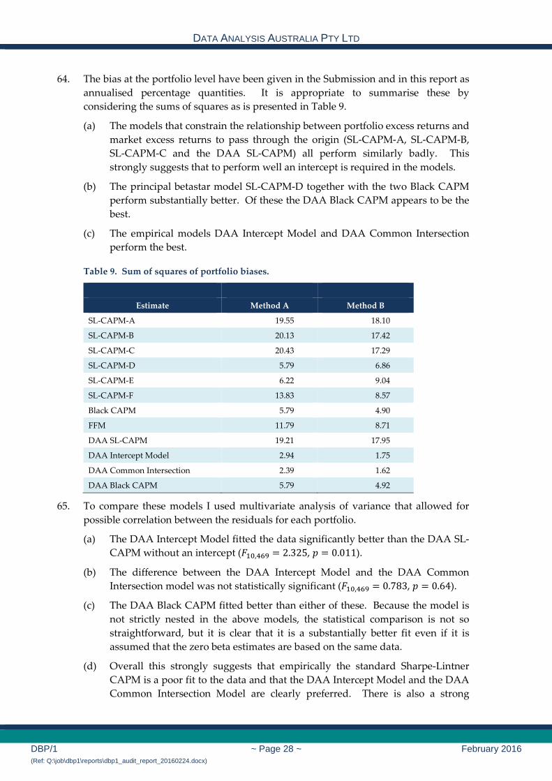
London, as an Accredited Statistician by the Statistical Society of Australia, and

as a Qualified Practicing Market Researcher by the Australian Market and

Social Research Society. Since 2003, I have been an Adjunct Professor of

Statistics within the School of Mathematics and Statistics of the University of

Western Australia.

(b) I am a Fellow of the Royal Statistical Society and a member of the Statistical

Society of Australia, the Australian Mathematical Society, the American

Statistical Association, the Institute of Mathematical Statistics, the International

Association for Statistical Computing, the Australian Society for Operations

Research, the Society for Industrial and Applied Mathematics, the

Geostatistical Association of Australasia and the Australian Market and Social

Research Society.

(c) I am current national Vice President (and acting President) of the Statistical

Society of Australia. I am also a past President of the Statistical Society of

Australia, the Geostatistical Association of Australasia and of the Western

Australian Branch of the Statistical Society of Australia. Between 2004 and 2010

I was a Member of the Accreditation Committee of the Statistical Society of

Australia and chaired the Committee between 2006 and 2010.



(d) Since 1988, I have been the Chief Consultant Statistician and Managing

Director of Data Analysis Australia, a firm I established to provide consulting

services in the areas of statistics and mathematics. Between 1983 and 1987, I

was a Senior Consultant with Siromath, a similar consulting company. Prior to

that I taught at the University of Western Australia in mathematics, statistics,

biometrics and quantitative genetics.

6. I consider that I have specialist knowledge in relation to the subject matter of this

report sufficient to enable me to provide an expert opinion on the matters set out in

this report.

7. I attach my curriculum vitae as Appendix C.

8. In preparing this report I was assisted by the following Data Analysis Australia staff:

(a) Dr Kathy Haskard, Senior Technical Consultant Statistician, BSc (Hons)

Adelaide, MSc La Trobe, PhD Adelaide, with over thirty years’ experience;

(b) Anna Munday, Principal Managing Consultant Statistician, BSc (Hons) UWA,

AStat, with over fifteen years’ experience; and

(c) Jennifer Bramwell, Consultant Statistician, BSc / BCom (Hons), MSc (Hons)

Auckland, with three years’ experience.

9. All worked under my direction and I wrote and take responsibility for this report in

its entirety.

Materials Provided 10. In preparing this report the materials provided to me from DBP were, in order of

receipt:

(a) “Submission 12 - Rate of Return Final“, and all the supporting Appendixes,

dated 2 November 2015.

(b) “Guidelines for Expert Witnesses in Proceedings in the Federal Court of

Australia – Practice Direction”, dated 6 November 2015, attached as

Appendix D.

(c) “Project Briefing Notes”, dated 17 November 2015, attached as Appendix A.

(d) “Proposed Revisions DBNGP Access Arrangement, 2016 – 2020 Regulatory

Period, Data and econometric code, Supporting submission 23”, via DropBox,

dated 25 November 2015.

(e) “Draft Decision on Proposed Revisions to the Access Arrangement for the

Dampier to Bunbury Natural Gas Pipeline 2016 – 2020” and supporting

appendix 4, 5, 6 dated 22 December 2015, received 23 December 2015.

(f) “Review Of Arguments On The Term Of The Risk Free Rate” by Martin Lally,

obtained 23 December 2015.

(g) “Brief for Extension of Scope”, dated 31 December 2015, attached as

Appendix B.



11. The code and data DBP provided to me for auditing purpose were, in order of

receipt:

(a) “Code and data for analysis (2014 version)”, obtained from Nick Wills-Johnson,

same as what was submitted to ERA, via DropBox, dated 25 November 2015.

(b) Supplementary data required for the 2014 version, obtained from Nick Wills-

Johnson after request, via multiple email.

(c) “Code and data for analysis (2015 version)”, obtained from Nick Wills-Johnson,

via Thumb drive, dated 12 January 2016.

12. In addition I have consulted the following papers:

(a) “Economic Forecasts and Expectations” by J Mincer and V Zarnowitz,

published 1969.

(b) “Industry costs of equity” by Eugene F. Fama and Kenneth R. French,

published 1997.

(c) “The Capital Asset Pricing Model: Theory and Evidence” by Eugene F. Fama

and Kenneth R. French, published 2004.

(d) “Estimating �: An update” by Olan T. Henry, April 2014.

(e) “National Gas Rules Version 28”, downloaded 17 December 2015 from

http://www.aemc.gov.au/Energy-Rules/National-gas-rules/Current-rules.

(f) “ERA Rate of Return Guidelines”, downloaded 15 January 2016 from

https://www.erawa.com.au/gas/gas-access/guidelines/rate-of-return-guidelines.

(g) “AER Rate of Return Guidelines”, downloaded 15 January 2016 from

https://www.aer.gov.au/networks-pipelines/guidelines-schemes-models-reviews/rate-

of-return-guideline.

13. I have also maintained email correspondence with Nick Wills-Johnson to receive

clarification regarding the DBP work and general Finance background as required.

Context 14. I understand that DBP has made a Submission to the ERA regarding methodological

issues in how to determine the most appropriate rate of return on their investments

in the Dampier to Bunbury Natural Gas Pipeline. I have been asked to restrict my

attention to Section 5, “Return on Equity”.

(a) These issues include the most appropriate Capital Asset Pricing Model

(CAPM) and how certain parameters in these models might be best estimated.

(b) The CAPM models claim to give a means of estimating an appropriate rate of

return in response to the level of risk involved in the investment. In general a

higher level of risk is compensated for by a higher expected rate of return.

(c) Risk is essentially defined as the uncertainty or unpredictability in the return.

This is usually measured using the statistical concept of the variance of the

distribution of returns.



(d) Risk is usually measured in terms of how the returns vary relative to the

market. To this end, the quantity “beta” (sometimes represented by the Greek

�) is defined as the average change in a return relative to a unit change in the

market. This is therefore equal to zero for a return that is uncorrelated with the

market, greater than zero for a return that moves in the same direction as the

market on average, equal to one if it moves the same as the market on average,

larger than one if it moves with the market but in a more extreme manner,

between zero and one if the movement is less strong than the market, and less

than zero if it moves against the market trend.

(e) The focus of the Submission is the most appropriate estimation of the

appropriate rate of return. The economic theory of capital asset pricing is a

means to this end, creating the need for the Submission consider the most

appropriate estimates of beta and how beta may be then used to determine an

appropriate rate of return commensurate with the risk.

(f) To this end DBP have presented both a methodological argument and an

analysis of data that it considers relevant to demonstrate that their proposed

methodology – model choice, model fitting and model use in prediction – is

more appropriate than that proposed by the ERA. Particular emphasis is given

in the Submission to the assessment of model validity or adequacy when used

in a predictive manner since this directly relates to the overall focus of

estimating the appropriate rate of return.

15. My review is limited to the statistical issues involved, and in particular:

(a) Whether the statistical methods are appropriate and have been properly

implemented;

(b) Whether the statistical models may be considered “adequate” according to

various standard tests;

(c) Whether the ERA comments in their Draft Decision on the statistical

procedures are appropriate; and

(d) Any other statistical issues that arise in this context.

Structure of This Report

16. The report considers:

(a) The role of linear models and linear statistical regression in the estimation of

parameters in such models, with a discussion of statistical measures of model

goodness of fit and model adequacy;

(b) The role of models and the particular economic models referenced in the

Submission, highlighting the regressions used in the models presented in the

Submission and the model adequacy measures used in the Submission;

(c) My empirical analysis of the data presented in the Submission which leads to

models which better fit the data and provide statistically improved predictions

of the risk premium; and



(d) Comments on the statistical comments of the Draft Decision.

17. The overall finding is that both the Submission and the Draft Decision use methods

that are not statistically ideal, some from a theoretical perspective and some from a

data perspective.

(a) The issues relate specifically to the inclusion or otherwise of intercept terms in

regression models. I understand that the statistical methods of both the

Submission and the Draft Decision are widely used in finance, but they

strongly conflict with standard statistical theory and practice.

(b) However, while the statistical methods of the Submission are less than ideal,

they do provide reasonable estimates of the appropriate risk premiums,

performing substantially better than those suggested by the ERA.

18. The alternative methods of estimating the rates of return that I present have parallels

with the models presented in the Submission and the Draft Decision but are

theoretically robust and, in my opinion, significantly better supported by the data.

19. Much of the discussion in this report involves statistical concepts and methods that

are so well established that it is not clear which references to give – the original

papers are not particularly accessible to the modern reader and the material is

covered to varying levels of detail in many undergraduate texts. As general

references I recommend Everitt, B.S. (1998), The Cambridge Dictionary of Statistics,

CUB, Cambridge and Kotz, S., Johnson N.L. and Read, C.B. (1982-89), Encyclopedia of

Statistical Sciences, Wiley New York.

Statistical Background

Linear Models and Prediction

20. The Submission and the Draft Decision both refer to various models to express the

relationship between appropriate returns on an investment and the associated risks.

(a) I understand that these models have certain justifications based upon economic

theories, particularly those related to optimal investments. I do not comment

upon those economic approaches.

(b) To a statistician the models can be considered as approximations to reality,

typically involving some simplifications. In this approach a model is judged by

its usefulness in making correct inferences or predictions.

21. A model typically has a structure that includes one or more parameters or

coefficients that must be estimated for the model to be useful.

(a) A linear model has a particularly simple structure. In the case of a model with

one input variable, it represents a relationship between that input variable

(here termed “�”) and the output variable (here termed “�”) in the form

� = � + ��

where � and � are parameters.



(b) The description of this model as “linear” refers to the manner in which

changing a parameter value changes the value of �, with the change in � being

precisely proportional to the change in the parameter.

(c) Linear models are not restricted to only one input variable x. Typically each

input variable will have its corresponding parameter equivalent to � above.

22. In practice the relationship between the input variable and the output variable will

often be imprecise due to errors in the data or to shortcomings in the model.

(a) This is often represented by introducing an “error term” in the model, so the

relationship can be given as

� = � + �� + �

where the term � represents a random quantity.

(b) Usually the term � is assumed to have certain statistical qualities, such as

having an average or expected value of zero and having a well defined

distribution, such as the normal distribution.

(c) The model given in 22(a) also makes an assumption on how the error term

interacts with the parameters. In particular this model assumes that the error

acts directly upon the output � and this action does not depend upon the

parameter values.

(d) There are a number of alternative models, one being of the form:

� = � + �� + ��. In this the effect of the error term � on the output � is affected by the value of�.

This model has different statistical properties and gives rise to what are called

“errors in variables” problems.

(e) It is possible to combine these models to incorporate more than one source of

error. For example, the model might be of the form:

� = � + �� + �� + �

Where � and � represent the two error terms. In general such models give rise

to difficult estimation problems.

(f) Some linear models may be assumed to have constraints on the parameters.

For example, in the above models it might in some circumstances be

appropriate to assume that the parameter a (often termed the “intercept”)

should be zero.

23. A typical application of a model is to predict what the output might be for a

particular value of the input. That is, for a particular value of � what will the value

of � be. For such applications it is necessary that the values of the parameters be

known. However in most cases the prediction will not be precisely correct.

(a) With the model given in 22(a), it will impossible to predict the value of the

error term �. This might be termed the intrinsic prediction uncertainty.



(b) In situations where the parameter values are not known with certainty,

estimates must be used. To the extent that the estimates are not the true values,

there may be some further uncertainty in the prediction. This might be termed

the estimation prediction uncertainty.

(c) In practice the prediction uncertainty, also known as the prediction error, is

usually a combination of these two forms of uncertainty.

(d) A final form of uncertainty relates to whether the model itself is appropriate.

While the prediction error as described above is well understood by methods

of mathematical statistics, the uncertainty due to an incorrect or approximate

model is usually less tangible.

Estimation and Regression

24. The estimation of these parameters is usually based upon the analysis of relevant

data. The precise estimation method will depend upon the statistical characteristics

of the model and the data.

(a) It is not unusual for there to be more than one estimation method for a given

parameter. Estimation methods will typically differ in the assumptions they

might make about the statistical characteristics of the data, their accuracy and

their tendency to have biases.

(b) While there are certain theoretical findings that some methods of estimation are

optimal in that they achieve estimates with minimal uncertainty, such findings

invariability depend upon the correctness of the assumptions and upon the

measure of uncertainty used.

25. The estimation methods used in this report for the analysis of the data are examples

of linear regression.

(a) Generally a linear regression model is of the form

� = � + �� + � where � is the dependent variable (also called the endogenous variable in

some economic contexts), � is the independent variable (also called the

exogenous variable in some economic contexts), � and � are parameters to be

estimated and � is a so-called error term. Here the index � indicates the �th

data value.

(b) Linear regression (sometimes called ordinary least squares or OLS) is a

standard procedure for estimating the coefficients � and �. Linear regression

usually makes several assumptions about the data, namely that the errors � have expected average value zero, that they are statistically independent of

each other and that they all follow the same normal distribution with a

common variance. Under these assumptions it can be shown by the Gauss-

Markov Theorem that linear regression gives optimal estimates of � and �.

These estimates are often denoted as �� and ��.

(c) In this case optimal means that the estimates �� and �� will not be biased and

they will have minimal variability as measured by the variance. The variance



is a commonly used measure of uncertainty of a quantity, being the average

squared departure from the average value.

(d) There is also an implicit assumption that the model given in 25(a) above is

correct, that is that the relationship between � and � is in fact linear.

(e) If these assumptions do not hold then the estimates �� and �� may no longer be

optimal and may be biased and non-optimal. In such circumstances the

models have the potential to be misleading.

Model Adequacy

26. In evaluating the quality of a model, it is common to:

(a) Consider the “goodness of fit” to the data used in estimating the parameters of

the model; and

(b) Compare predictions of the model with the actual values, using data beyond

that used to estimate the parameters.

27. The goodness of fit is usually considered in terms of the residuals � . These are

defined by the difference between the actual output values and the predicted output

values for the data used in fitting the model. That is

� =� − �� where

�� = �� + �� .28. The scale of the residuals is usually measured by the sum of squares ∑ � � and most

statistical methods that guide the selection of a model use this quantity.

(a) In particular, models can be compared by comparing their respective sum of

squares of residuals. There is a well-developed statistical theory of model

comparisons based upon this which can indicate whether differences in model

fit are likely to have arisen by chance or not.

(b) Such comparisons are usually made in the context of having a model that is a

simplified version of the second model. The comparison can indicate whether

the terms removed or constrained in the simplification process are statistically

significant. The common statistical test in this context is Fisher’s F-test.

(c) Here statistical significance refers to a low probability that the difference in the

residual sum of squares could have arisen by chance rather than being due the

terms being actually present in the data.

29. While the examination of residuals can highlight problems with a model, the fact that

they use the one data set to both fit the model and to evaluate it is often regarded as

providing less than ideal assurance that the model can be applied more generally.

(a) This concern has led to methods that either use additional data to validate the

adequacy of the model, or to use the one data set in more sophisticated ways.

While the terminology is not standardised in the statistical literature, such

methods can be called prediction analysis.



(b) The use of additional data is common in situations where there is ample data.

In such contexts it is not uncommon to have a “training” data set which is used

to fit the model and a “test” data set to evaluate it.

(c) An alternative is to use the one data set but repeat the model fitting process

many times, each time leaving out a subset of the data (most typically one

record) and then testing the fitted model on the subset left out. This is

approach is often called cross validation.

(d) Cross validation methods are particularly easily applied when the data

structure is simple so that removing part of the data does not affect the validity

of the data. They are more difficult to apply in more structured data such as

time series (data collected at regular intervals in time) where the omission of

some data may create gaps that affect the statistical structure. Recursive

methods in time series that use an expanding window on the data are

consistent with the cross validation approach.

30. In the prediction analysis, the prediction errors, or the differences between the

predictions and the actual values, should ideally be small. There are two aspects of

the prediction errors that are commonly considered:

(a) Whether the prediction errors are predominantly in one direction, commonly

termed a bias.

(i) Unbiasedness is often considered to be a highly desirable but not

absolutely essential property of estimators. In the context of linear

regression unbiasedness is usually not difficult to achieve provided that

the model is appropriate for the data. Hence in the case of linear

unbiasedness across a range of contexts is almost equivalent to model

adequacy.

(ii) Bias is typically assessed by a “t-test” as is further discussed below.

(iii) Where multiple assessments of bias are considered, it is rarely

appropriate to examine numerous possibly related t-tests. In such

situations omnibus tests such as the Wald test and Hotelling’s T test that

consolidate the t-tests into a single value is more appropriate. Such tests

are still concerned with bias.

(iv) In the case of linear regression models, the Wald test and Hotelling’s T

test are identical. The Wald test uses a quadratic approximation to the

likelihood function to provide a test of significance. In linear regression

the likelihood function is precisely quadratic and corresponds to a

natural multivariate extension of the t-test.1 In this form it is commonly

referred to as Hotelling’s T test.

(v) Such tests are only concerned with whether the bias is statistically

significant. A statistically significant bias might or might not have

practical significance.

1 Hotelling, H., (1931) The generalization of Student’s ratio, Ann. Math. Statist., 2,360-378.



(vi) Conversely, because the statistical test examines possible biases relative

to the inherent uncertainty in the data, if the inherent uncertainty is large

then the statistical test will have low power in detecting biases that may

actually be present. Therefore particular care must be taken with small

data sets as that will accentuate the problem of low power.

(b) Whether the prediction errors are spread out or highly variable.

(i) Even in the absence of a bias, it is still undesirable for the predictions to

be highly variable.

(ii) This variability is often measured by the standard deviation or the

variance of the prediction errors (“prediction error variance”).

(iii) Whilst statistical tests exist for comparing the variability against a

benchmark or similar criterion, typically F-tests, the frequent absence of

accepted benchmarks or criteria means that they are less frequently used.

31. A measure that combines both forms of error (bias and variability) is the mean

square prediction error – the average of the squares of the prediction errors. In many

contexts this provides a single measure that can be used to compare prediction

methods.

32. In some contexts other properties of the prediction errors might also be considered.

(a) It is common in applied statistical work to plot residuals or prediction errors

against other variables to explore if there is some systematic structure.

(b) A common plot is of the prediction errors against the predicted values,

typically used when non-linear relationships are suspected.

(c) The Mincer-Zarnowitz test is a formal test of model adequacy, specifically

testing for a linear relationship between predicted values and prediction errors.

That is, it tests for variability in the bias across the range of prediction values.

(d) The Mincer-Zarnowitz test is usually implemented by regressing the actual

values upon the predicted values for which the hypothesised regression line

will have an intercept of zero and a slope of one. It can be equivalently

implemented as a regression of the prediction errors on the predicted values in

which case the hypothesised regression line will have an intercept of zero and a

slope of zero. The test involves considering whether the estimated coefficients

collectively differ to a statistically significant amount from the hypothesised

values.

(e) While the Mincer-Zarnowitz test normally regresses the actual values only on

the predicted values, the regression need not be restricted to such terms. It can

be extended to include any terms to cover possible biases that are considered

either possible or critical, and can consider biases in particular subsets of the

data.



33. Care is required when interpreting the t test, the Wald test (and in this context the

identical Hotelling T test) and the Mincer-Zarnowitz tests.

(a) The tests consider biases relative to the variability in the predictions.

Furthermore the tests are mathematically interrelated.

(b) A low value of the test statistic can be due to a small bias or a high variability

or a combination of the two.

(c) The test statistics themselves do not quantify the magnitude of a bias.

(d) For these reasons it is common to also consider the mean square error, one that

combines the effects of bias and lack of precision.

Models in the Submission 34. The models refer to excess returns, which are returns on an investment above the

expected return on a risk free investment, typically an investment in government

guaranteed bonds.

(a) The Submission uses the Reserve Bank of Australia bond rate for the risk free

investment. I can make no comment upon whether this is an appropriate

choice, although I understand that it is consistent with common practice.

(b) The expected value of the excess return (abbreviated ER) on an investment is

referred to as the risk premium (abbreviated RP).

35. The Submission and the Draft Decision refer to three distinct models relating risk

premiums from a portfolio to risk premiums from the market overall:

(a) The Sharpe-Lintner Capital Asset Pricing Model (SL-CAPM),

portfolioRP = �marketRP; (b) The Black Capital Asset Pricing Model (Black CAPM),

portfolioRP = 1 − ��zerobetaRP + �marketRP; (c) The Fama French Model (FFM),

portfolioRP = & + �marketRP +��HML +�*SMB. 36. These three models have, respectively, one, one and four parameters. In each case

one parameter is termed “beta” or �.

(a) Beta is a measure of how the return from an investment moves with the overall

market (refer to Paragraph 14(d)). It can be considered to be the slope of the

relationship between the return on an investment and return in the overall

market.

(b) Implicit in each of the three models are assumptions on the nature of the

relationship between a portfolio’s returns and market returns.

(c) The Black CAPM is a variation of the SL-CAPM with an additional term

(explanatory variable, zero-beta risk premium) but a constraint between the

two coefficients, so it still has only one free parameter. It is a generalisation of



the SL-CAPM in that the SL-CAPM is equivalent to the Black CAPM with the

zero-beta risk premium set to zero.

(d) The FFM is a generalisation of the SL-CAPM, with an added intercept and two

additional terms (“High minus Low” and “Small minus Big”).

37. To apply each model, it is necessary to estimate the relevant parameters. There can

be several means of estimating the parameters and it is clear from both the

Submission and the Draft Decision that there are concerns amongst economists that

some methods might be biased, leading to several different estimates being

proposed.

(a) The estimation of parameters needs to be considered in the context of the

model itself. Different models can imply different assumptions about the data

and parameters.

(b) This is particularly the case with the beta parameters, since their precise

definition varies between models. Care must be taken to avoid general

definitions that do not clearly reference the assumptions or the context.

(c) For example, the value of beta coefficient in the Fama French model will be

affected by the additional terms in the model is those terms are correlated to

the market excess returns. Hence there is no statistical reason to expect that the

value of beta in the Fama French model would be similar to the value in (say)

the Black CAPM.

(d) In my opinion the Submission could have been clearer in this regard.

38. The Submission considers six estimates for the beta in the SL-CAPM.

(a) A simple linear regression estimate, described in the Submission as a “vanilla”

method. Note that the regression used in the Submission includes an intercept

as well as the slope (beta), so is not a true SL-CAPM regression which has no

intercept.

(b) A method that uses a similar regression but instead of using the central

estimate of beta uses the upper bound of the two-sided 95% confidence interval

for beta. This is described as using the 95% quantile (95th percentile) but is

actually associated with the 97.5% quantile or 97.5th percentile. In the

Submission this is termed the “ERA empirical SL-CAPM” as it is, I understand,

the approach of the ERA.

(c) A similarly modified estimate using the upper bound of the 99% confidence

interval. This is described as using the 99% quantile (99th percentile) but is

actually associated with the 99.5% quantile or 99.5th percentile. In the

Submission this is termed the “empirical SL-CAPM with the 99th percentile beta

estimate”.

(d) The “betastar” estimate that begins with the simple linear regression estimate

(Paragraph 38(a)) as if it was a Black CAPM estimate, but modifies it for use in

the SL-CAPM. The Submission provides a theoretical justification for this



based upon an algebraic reformulation of the Black CAPM. It is calculated

using the following formula

β/0∗2 =31 − 45674867 9 �:62 + 345674867 9

where �:62 is the estimated slope from the ordinary linear regression of portfolio

; excess returns on market excess returns over all available months � up to

month < − 1, 4=67 is the means of the zero-beta excess returns for all available

months � = 1 up to < − 1 and 4867 is an estimate of average monthly market

excess returns, calculated by a crude conversions from the average of the

annual market excess returns from a USA-based source, using >8? for year

@ = 11883� up to the latest complete year ended before month <, utilising C6 values where C6 = 80 + integerpart G6HII� J,

>86LLLLL = 1C6 M >8?

NO

?PI

and

4867 = 1 + >86LLLLL� II� − 1.

(e) A modified betastar estimate that uses the estimated 20th percentile of betastar,

namely the lower bound of a two-sided 60% confidence interval for the

expected value of betastar. It appears that the choice of the 20th percentile was

based on the lowest value whereby the model adequacy statistics were

acceptable.

(f) A modified betastar estimate that uses the estimated 99th percentile of betastar,

namely the upper bound of a two-sided 98% confidence interval for the

expected value of betastar. It appears that the choice of the 99th percentile was

based on the highest value whereby the model adequacy statistics were

acceptable, giving a range of possible values for betastar.

39. For convenience these six estimates will be referred to as the SL-CAPM-A through to

SL-CAPM-F estimates. These estimates and others referenced in this report are

summarised in Table 7 below.

40. The Black CAPM � is estimated by simple linear regression, giving the same estimate

of � as used for SL-CAPM-A.

(a) To produce forecasts, this estimate of beta is substituted directly into the Black

CAPM model, �:Q7 = R1 − �:62S45 +�:6248 .

(b) In a statistical sense the optimal (minimum variance unbiased) estimate of beta

could be easily obtained by regressing 4T6 − 45 � on 48 − 45 �, without an

intercept).

(c) For reasons that we will explore further in the report, the simple estimate of

beta is close to the optimum estimate.



41. The Fama French Model parameters including beta are estimated with an intercept

but applied without an intercept.

42. Several statistical comments can be made at this stage.

(a) In general, it is expected that models will perform best if the form of the model

equation on which parameters are estimated corresponds to the model

equation used to implement forecasts.

(b) Indeed, where different models are used to estimate parameters and to

implement forecasts there should be no automatic expectation that the

combination will perform well unless the data is statistically consistent with

both models. Typically this will require that:

(i) The model used for the forecasts is consistent with the data; and

(ii) The model fitted to estimate the parameters is an extension of the forecast

model, that is, containing additional but unnecessary terms that are

therefore likely to have a minimal effect of the parameter estimates.

(c) For example, suppose a linear model without an intercept term is consistent

with the data. Then it is possible to fit a linear model with an intercept term

and use the estimate of the slope from this in a model without an intercept,

since the estimated intercept will be statistically insignificant. However if the

linear model without an intercept is not consistent with the data then such a

process will lead to a significant bias in predictions.

43. None of the regressions fitted corresponds exactly to either SL-CAPM or Black

CAPM. The theoretical SL-CAPM has a zero intercept and is a regression through

the origin of portfolio excess returns on market excess returns. The Black CAPM also

has no intercept, but two explanatory variables with a constraint between the two

parameters, and is equivalent to a regression through the origin of “portfolio excess

returns minus zero-beta excess returns” on “market excess returns minus zero-beta

excess returns”.

(a) However for both SL-CAPM and Black CAPM the estimate of � was based on a

simple linear regression of portfolio excess return (ER) on market ER, with

intercept, namely

portfolioER = & + �marketER, which can be expected to be sub-optimal when applied in a different model.

(b) In all the SL-CAPM-based forecasts, the model assumed was the true SL-

CAPM, portfolioER = �marketER, but using an estimate �V calculated in some

way other than the statistically natural method of fitting the natural regression

of portfolio ER on market ER without intercept.

(c) In the Black CAPM-based forecasts, the model assumed was the true Black

CAPM, portfolioER = 1 − ��zerobetaER + �marketER, but using an estimate

�V calculated in some way other than the statistically natural method of fitting

the natural regression of “portfolio ER minus zerobeta ER” on “market ER

minus zerobeta ER”.



44. The Fama French Model was correctly fitted with an intercept, providing optimal

estimates of all the parameters including the intercept, but forecasts were derived

ignoring the intercept. Again, this is unlikely to produce optimal forecasts.

45. The inclusion of an intercept in the model fitted to derive estimates SL-CAPM-A, SL-

CAPM-B and SL-CAPM-C is surprising and can potentially lead to poor

performance.

(a) I would expect the SL-CAPM-A estimate of beta to be frequently biased

towards zero, that is, to be too small in magnitude, relative to the theoretical

SL-CAPM.

46. It appears that the justification for SL-CAPM-B and SL-CAPM-C is to overcome bias.

(a) If so, it is a badly flawed approach as it confuses the potential bias due to an

inappropriate model with the uncertainty or error in estimation as measured

by the confidence interval when the model is correct.

(b) The falsity of this approach is evident if the situation of an arbitrarily large

sample size is considered – the confidence interval would become arbitrarily

small resulting in an insignificant “correction”, but the bias which is not related

to the sample size would remain the same.

(c) If this approach gives seeming good forecasts in a particular situation, it would

still be difficult to justify as it would be a chance event. A larger sized sample

would give forecasts that performed less well since the bias “correction” would

be reduced.

47. The SL-CAPM-D estimate uses a different “bias-correction” approach, which is likely

to yield an estimate closer to the ideal SL-CAPM estimate, and hence might be

expected to perform better and have potentially smaller bias. I understand that this

method, termed the betastar method, has been developed for the Submission

(a) Effectively the method uses the regression with an intercept to estimate the

expected portfolio excess return at a nominated average market excess return

and then choses the value of betastar that ensures that the SL-CAPM predicts

this.

(b) The “corrections” of the SL-CAPM-E and SL-CAPM-F estimators are flawed in

the same way as the SL-CAPM-B and SL-CAPM-C estimators. However they

are primarily used to provide a range of potentially acceptable values of the

beta parameter of the SL-CAPM.

(c) The so-called delta method was used to determine the standard error of

betastar. The asymmetry of the SL-CAPM-E and SL-CAPM-F estimators, that

is the 20th and 99th percentiles, is a reflection of the skewness of the distribution

that was not captured by the delta method.

(d) The process by which the SL-CAPM-E and SL-CAPM-F estimators were

obtained, that is, a search across the percentiles of the confidence interval

distribution for the estimates of betastar that provide predictions that do not

display significant bias, weakens the conceptual link to the original estimate of



betastar. In principle any estimate for beta could have been used to start such a

search and hence the SL-CAPM-E and SL-CAPM-F estimators are actually

bounds on reasonable values of beta in the SL-CAPM-D.

Evaluation Framework Using Portfolios

48. To evaluate the adequacy of the models and the estimators, the Submission presents

a set of empirical results using Australian stock exchange data for major companies.

49. A set of portfolios was created using the following steps:

(a) For each company their beta was estimated for each month using the previous

five years of monthly data, for companies that have data for the previous ten

years.

(i) A linear regression model of stock return to market return was used to

estimate the beta for each stock.

(ii) However, the linear model has estimated intercept as well the slope

which conflicts with the beta as defined by the SL-CAPM but which is

consistent with the usage in other parts of the Submission.

(iii) In considering returns, adjustments are made to take into account factors

such as franked versus unfranked returns.

(b) Only stocks in the top 100 (before 1974) and top 500 (from 1974 onwards) as

defined by total market capitalisation are used for portfolio formation.

(c) For each year, 10 portfolios containing the same numbers of companies are

formed based on their betas for January that year.

(i) One implication of this is that a company may move from one portfolio to

another portfolio between years.

(d) Returns for portfolios for each month are calculated using total capitalisation,

using that of the current month relative to that of previous month.

(e) Then the values are adjusted using risk free rate as estimated by Reserve Bank

data, to provide excess returns.

50. Additional data was provided for each time period: annual market excess returns as

obtained from NERA, and derived monthly market excess returns.

51. The method used in constructing the portfolios can be expected to give ten portfolios

with a range of beta values and each portfolio being based upon sufficient stocks that

they will not be strongly affected by the idiosyncrasies of any single stock. In that

sense it appears to be a reasonable method of understanding how returns may relate

to betas in the Australian market.



Implementation

52. The analyses were implemented using the statistical program R and the associated

“R Markdown” package.

(a) R is a widely used statistical program described as “a language and

environment for statistical computing” and is produced under the auspices of

the R Foundation for Statistical Computing.

(b) R Markdown package works in conjunction with R to provide better control

over the formatting of the output. R Markdown input files, with the filename

extension “.Rmd” or “.rmd” were the principal programs examined in this

review.

(c) Much of the code, while presented in R, is acknowledged as a literal translation

of earlier SAS code.

(d) There is also some evidence that some manipulations of the data were carried

out in Excel. It is not possible to fully verify what was done in Excel as these

were manual rather than programmed steps.

(e) Specific files examined in detail were:

(i) Finding bias with Simons beta-sorted

portfolios_nowait_final version.rmd. This is the main file

where t-test, Wald test, Hotelling’s T test statistics and Mean Square

Errors for all the models are produced. From now on we will refer to it

as the Model Adequacy Test (MAT) code .

(ii) simon_betapf_nowait.csv. This is the input file for doing Model

Adequacy Tests for the SL-CAPM models A – C. It contains portfolio

excess returns for the 10 portfolios as well as two measures of market

excess returns.

(iii) GMM_MZ.Rmd. This implements the Mincer-Zarnowitz tests using the

generalised method of moments.

(iv) simon_betapf_4pics_nowait_newFFM.csv. This is the input file

for doing the Model Adequacy Test for the Black CAPM model and the

Fama French Model. In addition to the data in the

“simon_betapf_nowait.csv”, it also contains HML and SMB

variables for the FFM model, as well as the zero-beta portfolio excess

returns necessary for the Black CAPM model.

(v) simon_calc_recurbetastar_nowait.csv. This is the input file for

doing the Model Adequacy Test for the SL-CAPM models using betastar.

In addition to the data in the “simon_betapf_nowait.csv”, it contains

betastar estimates and estimates of standard deviations of betastar for all

10 portfolios.

(vi) BetaStarSASConversion.Rmd, the R code for calculating betastar and

its estimated standard error, for each of the ten portfolios, for January

1979 to December 2013.



(vii) SRCBET_SASConversion.csv, input data for monthly excess returns

for each of the ten portfolios, the market, and the zero-beta, for months

March 1963 to December 2013, although the portfolio and market data

has a number of missing values preceding January 1979. This was

derived from SIRCA data.

(viii) NERMRP_SASConversion.csv, input data for annual market excess

returns from NERA Economic Consulting, for years 1883 to 2013, and a

monthly version of an historical average of all the annual values prior to

the current year.

(f) A number of other files were also examined only to ensure that they were not

relevant to this review.

53. Several versions of the programs were provided, corresponding to:

(a) Programs supporting the 2014 Submission and using data up to and including

2013 (the “2014 Programs”);

(b) Programs subsequently supplied to the ERA in 2015 using data up to and

including 2014 (the “2015 Programs”). In general the changes from the 2014

Programs were minor, adjusting for the different numbers of rows in the data

files and correcting minor errors. The 2015 program also has code for

additional tests that was not included in the 2014 code, although their outputs

were available in the 2014 Submission; and

(c) Programs as modified by Data Analysis Australia to ensure they would run on

our computer systems (the “DAA Programs”). In general these were based

upon the 2014 Programs with minimal modifications to ensure that they were

compatible with the later versions of R that I used and that file conventions

were compatible with our systems.

54. The 2014 Programs and the 2015 Programs were not well documented and used poor

programming style, suggesting that they were originally developed for internal

purposes.

(a) Comments in the program files were minimal and not always helpful.

(b) The code was highly repetitive using repeated copies of code with minor

changes rather than using looping structures that are normally recommended.

This led to superficially long programs which could be off-putting to the

reader. While this is poor practice and is potentially error prone, I did not find

any errors due to this.

(c) The code refitted the same models many times, resulting in execution times

that were substantially longer than necessary. This was not necessarily a major

problem since most execution times were sufficiently manageable.

(d) The code reused or overwrote key quantities making verification of the

correctness of the code unnecessarily difficult.

(e) More seriously, some code was clearly changed between runs that were

presented in the Submission. In particular the code for betastar model at the



20th percentile is missing as I understand that the same code was repeatedly

run for different percentiles. The code as provided corresponded to the 99th

percentile.

(f) Some of the code was clearly converted from earlier versions designed to run

on the SAS statistical program. This led to various inefficiencies including

several steps that while not incorrect in R, were unnecessary.

(g) Despite the code being poorly structured, I found no errors associated with this

lack of structure with the exception of the following in the MAT code file:

(i) A typographic error where a value of 2.36 was used instead of 2.326 for

the 99th percentile of the normal distribution. The effect of this error is

small but it does make some comparisons more confusing than they need

be.

(ii) The code for calculating the t-test statistics for the Fama French Model

used data up to time < instead of < − 1 to estimate the coefficients. That

is, the data used to estimate the coefficients for prediction already

contains the actual return to be predicted. The effect of this is small.

(iii) The code for calculating the Wald test statistics for the SL-CAPM-E and

SL-CAPM-F failed to incorporate results from the first 60 time periods

(equivalent to first five years of estimates). The effect of this is detailed in

Table 1.

55. The implementation of the Mincer-Zarnowitz test uses the R package gmm that is

based upon the generalized method of moments.

(a) This is nominally a departure from the normal implementation of the Mincer-

Zarnowitz test, but the moment conditions used actually make it equivalent

with the exception of how the statistical significance is computed.

(b) No explanation has been provided for this approach but it appears that it was

used to account for the correlations between the prediction errors for differ

portfolios. If not for this correlation, the standard approach could use the R

function lm that provides for easier programming and much easier testing.

(c) The gmm package provides standard errors for the estimates of the coefficients

and an estimate of the corresponding covariance matrix. That allows for a

single test of the collective significance of the coefficients. However the

Submission only reports the individual coefficients with their standard errors,

without a formal test of significance.

(d) Despite the findings with other tests of model adequacy that the biases appear

to vary between portfolios, the Mincer-Zarnowitz test was implemented as a

test for a uniform bias across all the portfolios. This would greatly weaken the

statistical power of the test.

(e) While I was provided with code for the Mincer-Zarnowitz test set up for

application to the portfolio data for several estimation methods, the results

presented in the Submission table 13 did not match these results. It appears



that the R code was written to replicate previous calculations carried out in

SAS and to then compare the results with those from SAS. The results were

different and the Submission reports the SAS results.

Model Adequacy Tests in the Submission 56. The focus in the Submission is upon model adequacy in terms of prediction beyond

the data set used to fit the models.

(a) This corresponds to the prediction analysis as described in paragraph 30 above.

As such it avoids some of the shortcomings of only examining the residuals.

(b) The approach is to use an expanding set of data – data up to time < − 1, to fit

the model and to then test the prediction for time <. This constitutes one form

of cross validation that is well suited for application to time series. In my

opinion this is a reasonable approach.

(c) Each predictive modal was used with two possible inputs – the historical

average monthly market excess returns (called Method A) and actual monthly

market excess returns (Method B). Method A reflects the real life situation

where the future value of the market return must be estimated and hence

provides a more realistic assessment of model adequacy. Method B removes

this form of uncertainty and hence provides some insights on other aspects of

model performance.

(d) This approach generates a time series of prediction errors for each estimator

and each portfolio. Normally a time series would give concern that there may

be autocorrelation, with each prediction error correlated to the ones before it

and after it. Such autocorrelation has the potential to invalidate the test

statistics used for model adequacy in the Submission. This is not referenced in

the Submission. Consequently I examined the time series of prediction errors

for autocorrelation using both estimates of the autocorrelation function and of

the power spectra. For all time series it was evident that autocorrelation was

not significant and would not affect the validity of the test statistics.

57. I have replicated the analysis given in the Submission and with the exception of the

minor coding errors referenced above, my calculations agree with the Submission

with the following exceptions:

(a) The values of the Wald statistic for models SL-CAPM-E and SL-CAPM-F are, I

believe, incorrect in the submission. The Submission and the true values are

given in Table 1 below.

Table 1. Betastar percentiles, Wald test statistics output obtained from DAA,

corresponding to Table 12 in the Submission.

20th percentile 99th percentile

Method A Method B Method A Method B

DBP Submission 12 11.637 13.398 9.935 7.265

DAA calculated value 11.635 21.158 9.820 11.150



(b) The results for the Fama French Model presented in Table 9 of the Submission

have several errors. We understand that an attempted correction was included

in a subsequent Submission (as referenced in 10(d)), but this was also incorrect.

What we believe to be the correct values are given in below.

Table 2. Fama French Model – corrected Wald and t-test results, corresponding to Table 9

in the Submission.

Method A Method B

Wald test 16.000 16.095

Portfolio betaMRP betaHML betaSMB Mean

forecast error

T tests Mean

forecast error

T tests

1 0.626 0.071 0.304 -3.67% -1.492 -4.31% -2.322

2 0.720 0.255 0.083 -2.09% -0.788 -2.80% -1.533

3 0.724 0.225 0.112 -1.67% -0.623 -2.26% -1.308

4 0.827 0.251 0.072 -2.95% -1.026 -3.94% -2.363

5 0.920 0.197 0.019 -0.41% -0.127 -1.19% -0.673

6 0.955 0.188 -0.026 0.98% 0.306 -0.04% -0.028

7 1.034 0.234 0.030 3.88% 1.101 2.78% 1.634

8 1.209 0.043 -0.057 3.09% 0.797 1.66% 0.863

9 1.323 -0.158 -0.002 5.79% 1.354 3.95% 1.702

10 1.435 -0.101 0.326 5.42% 1.029 3.55% 0.978

58. In Tables 6 to 12 of the Submission the results of the t-tests and the Wald tests are

presented using this approach.

(a) As noted above, the code used in the Submission calculated both the Wald and

Hotelling T tests, but these, as expected, gave identical values. Hence what is

described as a Wald test in the Tables could equally be described as the

Hotelling T test.

(b) The critical (5%) value for the Wald test with 10 degrees of freedom is 18.3,

while the expected value under the hypothesis of no bias is 10.0.

(c) The critical value is exceeded for the SL-CAPM-A, SL-CAPM-B and SL-CAPM-

C estimates with both Methods A and B. I do not regard this as surprising

since they all involve a statistically questionable combination of a simple linear

regression with an intercept to estimate the slope in a model without an

intercept, with the “corrections” in SL-CAPM-B and SL-CAPM-C lacking a

statistical basis.

(d) Several of the other models, namely the SL-CAPM-D, SL-CAPM-E, SL-CAPM-F

the Black CAPM and the FFM are not above the critical value.

Additional Models

59. As stated in Paragraph 43, the estimator SL-CAPM-A is based upon linear regression

without the regression line being constrained to pass through the origin, while the

SL-CAPM does assume such a constraint. As a means of better understanding the



implications of this, two further models were fitted that provide statistical

consistency between the estimation step and the prediction step:

(a) A regression model constrained to pass through the origin, that is, with the

intercept fixed at zero. The results of this approach are presented in Table 3,

with the same performance measures as used for other six estimators in the

Submission. I term this the DAA SL-CAPM estimator.

Table 3. Summary prediction performance for the DAA SL-CAPM estimator.

Method A Method B

Wald test

26.340 29.829

Portfolio Betas

Mean

forecast error t statistic

Mean


1 0.543 -4.66% -2.000 -5.32% -2.903

2 0.614 -4.57% -1.863 -5.30% -2.937

3 0.581 -4.11% -1.638 -4.83% -2.768

4 0.774 -4.51% -1.707 -5.31% -3.195

5 0.866 -2.36% -0.779 -3.24% -1.880

6 0.886 -0.85% -0.284 -1.89% -1.257

7 0.966 1.80% 0.538 0.75% 0.438

8 1.179 2.44% 0.633 1.05% 0.558

9 1.354 7.54% 1.702 5.86% 2.510

10 1.377 6.32% 1.157 4.64% 1.217

(b) An alternative where the regression is not constrained to pass through the

origin (the intercept can be non-zero) and the prediction is made using this

intercept as well as the slope (beta). The results of this approach are presented

in Table 4, with the same performance measures as used for other estimators in

the Submission. I term this the DAA Intercept Model and estimator.

Table 4. Summary prediction performance for the DAA Intercept estimator.

Method A Method B

Wald test 5.971 6.187

Portfolio Betas

Mean


Mean


1 0.536 -0.11% -0.047 -0.78% -0.413

2 0.608 -0.27% -0.108 -1.01% -0.542

3 0.576 -0.25% -0.097 -0.97% -0.544

4 0.766 1.13% 0.415 0.31% 0.180

5 0.857 4.14% 1.328 3.22% 1.815

6 0.882 2.32% 0.765 1.28% 0.836

7 0.966 1.42% 0.424 0.38% 0.221

8 1.182 -0.19% -0.049 -1.54% -0.826

9 1.362 1.40% 0.324 -0.22% -0.097

10 1.384 1.20% 0.225 -0.44% -0.118



Figure 1. The fitted relationships for the ten portfolios in the DAA Intercept Model (in

black). The red lines correspond to zero excess returns and the green diagonal line to

portfolio excess return equalling the market excess return. (Note that these are not security

market lines – the slopes of the lines are the portfolio betas.)

60. The fitted lines for each of the ten portfolios using the DAA Intercept Model are

shown in Figure 1.

(a) Of particular note is that the ten fitted relationships appear to all pass very

close to a single point that is in turn close to the diagonal line where portfolio

excess returns equal market excess returns.

(b) This observation suggests a further model where all the individual portfolio

fitted lines are constrained to pass through a point on this diagonal. This is

similar to the SL-CAPM model but with an offset. Hence I have fitted such a

model, which I shall call the DAA Common Intersection Model. The results of

this approach are presented in Table 5, with the same performance measures as

used for other estimators in the Submission.

(c) I recognise that the DAA Common Intersection Model could be interpreted as a

special case of the Black CAPM with a constant zero-beta portfolio risk

premium. I am not able to comment upon whether such a model is sensible

from an economics perspective, but from a statistical perspective such a model

is clearly a very good representation of the structure of the data. I note that the

-0.10 -0.05 0.00 0.05 0.10

-0.1

0-0

.05

0.00

0.05

0.10

Market Excess Return

Por

tfolio

Exc

ess

Ret

urn



common intersection point corresponds to a return of 0.955% per month or 12%

per annum.

Table 5. Summary prediction performance for the DAA Common Intersection estimator.

Method A Method B

Wald test

5.105 5.394

Portfolio Betas

Mean


Mean


1 0.537 0.50% 0.211 -0.16% -0.086

2 0.608 -0.21% -0.086 -0.94% -0.510

3 0.577 0.63% 0.247 -0.09% -0.049

4 0.762 -1.95% -0.727 -2.74% -1.626

5 0.851 -0.77% -0.253 -1.64% -0.942

6 0.879 0.49% 0.162 -0.54% -0.356

7 0.967 2.19% 0.655 1.15% 0.673

8 1.183 0.34% 0.090 -1.01% -0.541

9 1.365 3.22% 0.742 1.57% 0.685

10 1.385 1.80% 0.336 0.14% 0.036

61. An appealing fourth additional model is the DAA Black CAPM fitted using the zero-

beta excess returns data provided, regressing “portfolio excess return minus zero-

beta excess return” on “market excess return minus zero-beta excess return”,

constrained to pass through the origin. The zero-beta return is similarly used in the

equation to predict for portfolio excess returns.

(a) The results of this approach are presented in Table 6, with the same

performance measures as used for other estimators in the Submission. I term

this the DAA Black CAPM and estimator.

Table 6. Summary prediction performance for the DAA fitting of the Black CAPM

estimator.

Method A Method B

Wald test

8.733 9.933

Portfolio Betas

Mean


Mean


1 0.538 -1.43% -0.604 -2.10% -1.126

2 0.607 -1.88% -0.756 -2.61% -1.425

3 0.576 -1.19% -0.467 -1.91% -1.076

4 0.768 -2.93% -1.098 -3.72% -2.217

5 0.859 -1.40% -0.461 -2.28% -1.314

6 0.882 -0.06% -0.019 -1.09% -0.721

7 0.965 2.02% 0.605 0.98% 0.572

8 1.181 1.09% 0.286 -0.27% -0.143

9 1.363 4.81% 1.100 3.15% 1.365

10 1.384 3.45% 0.640 1.78% 0.474



Comparison of Models

62. The Submission presents the results of the model adequacy tests across a number of

tables. The sequence in which they are calculated in the R code (across two files)

does not match the Submission or the order which we discussed them above. To

assist an understanding of this I have summarised the references in Table 7 below.

(a) The table gives the method of estimation and the method of predicting excess

returns, the key features that distinguish between the models.

(b) For the models considered in the Submission, the relevant tables of

performance in the Submission.

(c) The Wald statistics are given for the biases in all the models. In the cases

where the DBP Submission values are incorrect, the corrected values are given.

63. The Submission also provides mean square prediction errors (Table 14 of the

Submission) but without sufficient precision to be useful. I have recalculated these

for both the models presented in the Submission and the further models presented

here. The results, scaled by a factor of 10,000 for readability, are shown in Table 8

below.

(a) It can be seen that the mean square errors are uniformly higher for Method A

that uses historical data to forecast the marker excess return, whereas Method B

that uses the actual market excess return has a substantially lower excess

return. This is a commonly reserved result and reflects the added uncertainty

when using an estimated marker return, the situation that is relevant to

predicting future portfolio returns.

(b) Method B indicates that even when the market excess return is known, there is

still considerable uncertainty in the predictions. While this would be of

concern if the prediction was just to be carried out for one month, in practice it

is applied to several years and hence the bias which would affect the return

over such an extended period is much more relevant.



Table 7. Summary of the models considered in this report, with references to the relevant

tables in the Submission (items market † below are corrected by DAA as appropriate).

Wald Test

Model/Estimate Origin Estimation of beta Prediction Tables in

Submission

A B

SL-CAPM-A DBP Simple regression

with intercept

No intercept 10 26.766 29.792

SL-CAPM-B DBP/ERA Simple regression

with intercept, 97.5%

quantile

No intercept 6 24.910 25.821

SL-CAPM-C DBP Simple regression

with intercept, 99.5%

quantile

No intercept 7 24.355 24.557

SL-CAPM-D DBP Beta star Nominally no

intercept

11, 12 8.733 9.379

SL-CAPM-E DBP Beta star 20%

quantile

Nominally no

intercept

12 11.635† 21.158†

SL-CAPM-F DBP Beta star 99%

quantile

Nominally no

intercept

12 9.820† 11.150†

Black CAPM DBP Simple regression

with intercept

Black CAPM 8 8.733 9.880

FFM DBP Multiple regression

with intercept

No intercept 9 16.000† 16.095†

DAA SL-CAPM DAA Simple regression

without intercept

No intercept 26.340 29.829

DAA Intercept

Model

DAA Simple regression

with intercept

With intercept 5.971 6.187

DAA Common

Intersection

DAA Constrained to

common intersection

Through

common

intersection

5.105 5.394

DAA Black

CAPM

DAA Direct black CAPM Black CAPM 8.733 9.933



Table 8. Mean square Prediction errors for each model, method and portfolio, together with the mean for each portfolio. Scaled by a factor of 10,000

relative to those in the Submisson.

Portfolio

Model Method 1 2 3 4 5 6 7 8 9 10 Mean

SL-CAPM-A A 16.69 18.45 19.16 21.37 27.22 26.22 32.01 42.24 53.70 82.34 33.94

B 10.47 10.21 9.51 8.69 9.04 6.73 8.50 10.27 15.27 40.64 12.93

SL-CAPM-B A 16.65 18.41 19.13 21.34 27.19 26.21 32.02 42.26 53.76 82.43 33.94

B 10.59 10.18 9.18 8.82 8.97 6.58 8.37 10.23 15.48 41.08 12.95

SL-CAPM-C A 16.64 18.40 19.12 21.33 27.19 26.20 32.02 42.26 53.78 82.46 33.94

B 10.72 10.26 9.15 8.92 9.01 6.59 8.37 10.26 15.61 41.40 13.03

SL-CAPM-D A 16.58 18.33 19.04 21.30 27.20 26.20 32.01 42.21 53.46 82.14 33.85

B 15.62 12.91 10.96 9.55 8.90 6.45 8.40 11.65 18.08 44.12 14.66

SL-CAPM-E A 16.63 18.40 19.09 21.33 27.22 26.22 32.01 42.21 53.39 82.08 33.86

B 12.26 10.66 8.85 8.69 8.67 6.34 8.42 12.65 21.52 48.37 14.64

SL-CAPM-F A 16.59 18.26 19.03 21.23 27.15 26.18 32.02 42.24 53.75 82.41 33.88

B 36.50 29.01 29.34 15.17 11.12 8.31 8.75 10.38 15.71 40.78 20.51

Black CAPM A 16.58 18.33 19.04 21.30 27.20 26.20 32.01 42.21 53.46 82.14 33.85

B 10.33 10.06 9.36 8.58 8.99 6.70 8.49 10.28 15.11 40.53 12.84

Fama-French Model Method A 18.33 20.85 21.25 24.83 30.10 29.31 34.94 42.52 50.66 77.04 34.98

B 10.55 10.00 8.92 8.51 9.13 6.81 8.28 10.57 15.21 37.19 12.52

DAA SL-CAPM with no

intercept

A 16.68 18.45 19.16 21.37 27.22 26.22 32.01 42.24 53.70 82.33 33.94

B 10.47 10.16 9.44 8.67 9.00 6.69 8.49 10.28 15.26 40.61 12.91

DAA Intercept Model A 16.61 18.46 19.12 21.32 27.31 26.33 32.12 42.29 53.32 82.08 33.90

B 10.34 10.12 9.39 8.52 8.99 6.72 8.53 10.31 15.13 40.73 12.88

DAA Common Intersection

0.00955

A 16.53 18.26 19.00 21.25 27.16 26.18 32.00 42.20 53.38 82.06 33.80

B 10.27 9.99 9.31 8.53 8.98 6.69 8.48 10.28 15.05 40.48 12.81

DAA Black CAPM A 16.58 18.33 19.04 21.30 27.19 26.20 32.01 42.21 53.46 82.14 33.85

B 10.33 10.04 9.34 8.59 8.99 6.69 8.49 10.29 15.11 40.52 12.84



64. The bias at the portfolio level have been given in the Submission and in this report as

annualised percentage quantities. It is appropriate to summarise these by

considering the sums of squares as is presented in Table 9.

(a) The models that constrain the relationship between portfolio excess returns and

market excess returns to pass through the origin (SL-CAPM-A, SL-CAPM-B,

SL-CAPM-C and the DAA SL-CAPM) all perform similarly badly. This

strongly suggests that to perform well an intercept is required in the models.

(b) The principal betastar model SL-CAPM-D together with the two Black CAPM

perform substantially better. Of these the DAA Black CAPM appears to be the

best.

(c) The empirical models DAA Intercept Model and DAA Common Intersection

perform the best.

Table 9. Sum of squares of portfolio biases.

Estimate Method A Method B

SL-CAPM-A 19.55 18.10

SL-CAPM-B 20.13 17.42

SL-CAPM-C 20.43 17.29

SL-CAPM-D 5.79 6.86

SL-CAPM-E 6.22 9.04

SL-CAPM-F 13.83 8.57

Black CAPM 5.79 4.90

FFM 11.79 8.71

DAA SL-CAPM 19.21 17.95

DAA Intercept Model 2.94 1.75

DAA Common Intersection 2.39 1.62

DAA Black CAPM 5.79 4.92

65. To compare these models I used multivariate analysis of variance that allowed for

possible correlation between the residuals for each portfolio.

(a) The DAA Intercept Model fitted the data significantly better than the DAA SL-

CAPM without an intercept (WI5,XYZ = 2.325, ] = 0.011).

(b) The difference between the DAA Intercept Model and the DAA Common

Intersection model was not statistically significant (WI5,XYZ = 0.783, ] = 0.64).

(c) The DAA Black CAPM fitted better than either of these. Because the model is

not strictly nested in the above models, the statistical comparison is not so

straightforward, but it is clear that it is a substantially better fit even if it is

assumed that the zero beta estimates are based on the same data.

(d) Overall this strongly suggests that empirically the standard Sharpe-Lintner

CAPM is a poor fit to the data and that the DAA Intercept Model and the DAA

Common Intersection Model are clearly preferred. There is also a strong



suggestion that the DAA Black CAPM Model performs particularly well,

although the interpretation of this may be affected by the dependence on how

the zero beta values were estimated.

Review of the Draft Decision 66. In Paragraphs 1022 to 1025 the Draft Decision discusses the “bias-variance trade-off”,

referring to Chapter 6 of a standard reference The Elements of Statistical Learning by

Hastie, Tibshirani and Friedman. It is not clear how this relates to the criticisms of

the Submission.

(a) The reference is primarily concerned with non-parametric solutions to non-

linear problems where it is not possible to achieve unbiased estimators with a

finite sized data set. In such cases there is genuine need to counterbalance the

detail of a model as might be measured by the effective number of parameters

with the statistical stability of the results. Figure 15 of the Draft Decision is a

simple illustration of this where the tuning parameter might be the degree of

smoothing applied when estimating a curve.

(b) It is important to note that the reference focuses on situations where the true

model is not known and where the effective number of parameters (degrees of

freedom) in a fitted model can be quite large, even in the hundreds or

thousands.

(c) The models considered in the Submission and in the Draft Decision are by

comparison assumed to be of known form, to be by statistical measures quite

simple and linear. The models all have similar numbers of parameters. The

biases discussed in the Submission essentially come from the possible choice of

an inappropriate models for the data and no attempt is made to reduce biases

by making the models more complex.

(d) Hence the criticisms concerning bias-variance trade-off are not relevant to the

models discussed in the Submission. It is also not clear where the Draft

Decision uses the points raised in this section.

67. In paragraphs 1026 to 1042 the Draft Decision criticises the approach to model

adequacy in the Submission.

(a) In paragraph 1028 the Draft Decision outline the main issues as:

(i) The test does not evaluate prediction bias as claimed by DBP, only

overall prediction accuracy which is comprised of irreducible, bias and

variance components.

(ii) The test does not include uncertainty of prediction estimates within the

test.

(iii) The testing of each portfolio through the use of a t-test will suffer from

the multiple comparison problem, which will increase with the number

of portfolios.



(iv) The method of generating predictions potentially suffers from

pseudoreplication.

(v) The t-test is not specified, and for discussion purposes it is assumed to be

a two-sample t-test. In contrast, a paired t-test is a uniformly more

powerful test in discriminating differences between two dependent

samples of data.

(vi) The model adequacy test described is not de rigueur in the statistical

literature for assessing model performance, with no reference in the

literature in defence of the method cited by the authors.

(b) I will now address these issues.

68. I find the claim that the Submission does not address bias but only overall prediction

accuracy surprising, when the focus of the Submission is almost wholly is on bias.

(a) My understanding is that the overarching aim is to estimate appropriate rates

of return. The beta parameters are simply a step in this estimation process and

hence the Submission focuses on biases in predictions rather than biases in

estimates of beta.

(b) The summary results for each model provide an estimate of bias for each

portfolio and a t-statistics to allow evaluation of the statistical significance at

this level.

(c) The Wald statistics summarise these portfolio level measures of bias in the

statistically correct manner.

(d) The Draft Decision, especially in paragraph 1029, appears to have concerns

about the particular sources of bias and perhaps the effect of the uncertainty in

the estimation of model coefficients. In the context of the Submission, where

the data used to test the predictions is closely related to the data used to fit the

models, the principal source of bias will always be the inadequacy of the

models to fit the data, described in paragraph 1031 as the Type III error. The

Submission itself and my further analysis have both shown that the choice of

model and how it is used to predict returns is a substantial issue where

different models have quite different bias properties. However it is not clear

what the concerns of the Draft Decision might be beyond this.

69. In paragraph 1030 the Draft Decision references an “Appendix 1” and to the paper of

Henry “Estimating �: an update”:

(a) It is not clear what report that appendix may be part of.

(b) The Henry paper references the optimality of estimates of beta using the Best

Linear Unbiased Estimator (BLUE) criterion. The Henry paper does not make

it clear under what circumstances the simple linear regression (OLS) estimate

of beta is unbiased. In particular Equation (1) of Henry representing the

Sharpe-Lintner CAPM

a� � = �b + �caR�8 − �bSd Is essentially the same as Equation (4) of Henry,



� 6 = &�e6 + � 6 but with expectations. This implicitly assumes that aR�bS = &.

(c) However if the risk free rate �bis known, then the BLUE for � is no longer that

given by the simple linear regression with an intercept – the BLUE is the

regression without an intercept.

(d) In paragraph 1031, second dot point, the Draft Decision recognises that the

Henry approach can effectively estimate aR�bS. Indeed the reference to “type

III errors”, that is, that the model itself is incorrect is a good reason to follow

such an approach, highlights the benefit of having models that embody

sufficient flexibility to overcome problems of assumptions not being met.

(e) If the Henry approach does permit the estimation of the expected risk free rate

aR�bS, then the regression of the “raw” returns – that is the portfolio and

market returns not adjusted for the risk free rate – should give similar results to

the regressions presented here and in particular the DAA Intercept Model with

the intercepts differing by the average risk free rate for every portfolio. I have

conducted such regressions and the change to the intercepts is not uniform

across the portfolios as is shown in Table 10.

(f) The � quoted in Table 10 are obtained by regressing using all available data

(480 months), unlike the averages over an expanding window as given in the

Submission.

Table 10. Comparison of the DAA Intercept Model with the Henry Regression

Model.

DAA Intercept Henry Difference

Portfolio Intercept Beta Intercept Beta Intercept Beta

1 0.00409 0.5415 0.00738 0.5411 0.00329 -0.0005

2 0.00347 0.6238 0.00612 0.6278 0.00265 0.0040

3 0.00321 0.6529 0.00569 0.6538 0.00248 0.0009

4 0.00416 0.7949 0.00560 0.7974 0.00144 0.0026

5 0.00271 0.9308 0.00315 0.9355 0.00044 0.0047

6 0.00118 0.9472 0.00153 0.9502 0.00034 0.0030

7 -0.00121 1.0484 -0.00158 1.0508 -0.00037 0.0024

8 -0.00105 1.2168 -0.00258 1.2144 -0.00153 -0.0024

9 -0.00409 1.3453 -0.00652 1.3415 -0.00243 -0.0038

10 -0.00296 1.3875 -0.00567 1.3814 -0.00271 -0.0061

(g) This strongly suggests that the justification given by Henry for the using the

intercept in the estimation for beta in the Sharpe-Lintner CAPM does not apply

to this data.



70. In paragraph 1033, the Draft Decision raises concerns about multiple comparisons in

the context where the Submission gives results for the ten portfolios.

(a) The concerns of the Draft Decision are appropriately addressed in the

Submission by the use of the Wald statistics that combines the ten t-tests into a

single statistic, thus avoiding the problem of multiple comparisons. This

approach is both more statistically powerful and more accurate than the

Bonferroni method suggested by the Draft Decision since it is able to take into

account the correlation structure between the portfolios.

(b) The individual t-statistics are, in my opinion, very useful in understanding the

nature of biases once the Wald statistic has indicated that the overall bias may

be statistically significant.

71. In paragraph 1034 the Draft Decision raises concerns about pseudo replication. This

is a valid concern that was not explicitly addressed in the Submission. However the

tests that I have carried out for autocorrelation suggest that there is no need for this

concern.

72. The remarks about t-tests in paragraph 1035 of the Draft Decision correctly identify

the t-test being applied to the differences between the model predictions and actual

values. This might be termed a paired test, the pairs the predicted and actual values,

or one sample test, the values being the differences.

(a) The Draft Decision points out the need to properly take into account the

dependence between the “two samples” when carrying out such a test. The

Submission does this by directly calculating the standard error of the pairwise

differences and hence the tests in the Submission are the most powerful tests in

this context.

(b) Apart from clarifying this point (which may have led to the curious remark on

the Diebold-Mariano test in paragraph 1036), this remark does not appear to

raise any substantive issues.

73. In paragraph 1036 the Draft Decision claims that the use of the t-test and the Wald

test in this context “is not explicitly referenced in the statistical literature”.

(a) I find this comment curious as the highly generic t-test, as used here, is very

standard and totally appropriate for use here.

(b) Similarly the Wald test is a generic tool and is used appropriately here,

although the statistical literature in this context of linear models and implicit

assumptions of normality, it would be referred to as Hotellings T test. (It is the

natural multivariate extension to the t-test.)

(c) I would strongly disagree with the contention that the Mincer-Zarnowitz test is

more appropriate in this context. In particular the global form of the test, as

implemented in the Submission, lacks any power for the structured biases

likely to be encountered with the models considered here. In contrast, the

Wald test clearly identified problematic biases.



(d) The issue of pseudo replication raised again is not relevant for the reasons I

give above.

74. In paragraph 1037 of the Draft Decision reference is made to theoretical models

including the Sharpe-Lintner CAPM to “be more biased in their predictions than

their empirical counterparts”. The work contained in the Submission and analysis I

have carried out supports this statement.

75. In paragraphs 1043 to 1055 of the Draft Decision a discussion of cross validation

methods is presented with the suggestion that they should have been used in the

Submission.

(a) Cross validation is an accepted part of statistical practice and has enabled

statisticians to handle certain problems far better than more traditional

methods. It is a computationally intensive approach and hence has only come

to the fore in recent years when the required computational power has been

readily available.

(b) It is a method that, in a similar manner to the bootstrap, can be applied as a

black box to a variety of problems by repeated the calculations leaving out

subsets of the data each time. This is particularly useful when the analytic

methods of accessing models are impractical due to the complexity of the

mathematics.

(c) Cross validation is always problematic in the time series context since leaving

data out creates gaps that create theoretical and practical problems. One

method that avoids gaps is the expanding window approach that is used in the

Submission (and by Henry in his “recursive” estimates”).

(d) For linear regression models computationally efficient methods of

implementing cross validation have been available since the 1970s, making use

of standard matrix algebra. Despite this cross validation has never been a

preferred method in this context. Methods such as the Akaike Information

Criterion (AIC) and its derivatives have been preferred as being simpler and

just as good.

(e) The example of its use given in the Draft Decision – determining an optimal

window in time series forecasting – is a mathematically more complex situation

where the absence of practical analytic methods means that cross validation is

appropriate. In that sense the example is not relevant to comments on the

Submission.

Conclusions 76. In summary, I have found statistical shortcomings in both the Submission and the

Draft Decision. However the shortcomings of the Submission do not, in my opinion,

materially affect the reliability of predictions of excess returns and hence appear to

provide a reasonable basis for setting a risk premium. The shortcomings of the Draft

Decision appear to have, from a statistical viewpoint, a high likelihood of poor

predictions of returns and subsequently inappropriate estimates of risk premiums.



77. I have made all the inquiries that I believe are desirable and appropriate and no

matters of significance that I regard as relevant have, to my knowledge, been

withheld from this Report.

Dr John Henstridge

CStat, AStat, AFAIM, QPMR

24 February 2016


DBP/1 February 2016 (Ref: Q:\job\dbp1\reports\dbp1_audit_report_20160223.docx)

Appendix A – Project Briefing Notes

L\317347396.1

Every five years, DBP files a proposed Access Arrangement with the Economic Regulation Authority of Western Australia which contains, among other things, proposals for an appropriate return on equity for DBP’s equity owners. In its proposal filed on 31 December 2014, DBP developed a model of the statistical forecast bias of different asset pricing models when their projections are compared with subsequent actual returns over a sufficiently long timeframe. Now, DBP seeks an independent expert's opinion following a review of the statistical work undertaken as part of this modelling. In particular DBP seeks:

1. An assessment of the work undertaken and your opinion as to whether or not the calculations are accurate.

2. An assessment of the technical statistical work and your opinion as to whether or not that work was undertaken to a best practice standard.

3. An assessment of DBP’s findings from the statistical work undertaken and your opinion as to whether or not the findings represent sound, robust conclusions given the evidence in the empirical analyses.

We will provide you with:

The original data.

All regression codes and manipulations of the data we produced.

All our final outputs. The original data are supplied on a commercial-in-confidence basis and must be returned to DBP or destroyed upon completion of the assignment. Since it is possible that your expert report may be relied on in future proceedings before the Australian Competition Tribunal, we require that the work be undertaken in accordance with the Federal Court Guidelines for Expert Witnesses (attached). Please provide a quotation for this work which represents a capped fee, with check-points during the work such that, should the work be less than the capped fee, DBP will be liable only for costs incurred. Please also provide an indication of your hourly rates, in the event that, by mutual agreement, the above scope of work is expanded.



Appendix B – Brief for Extension of Scope

Statistical issues with respect to the Model Adequacy Test In its Draft Decision on Proposed Revisions to the Access Arrangement for the Dampier to Bunbury

Natural Gas Pipeline 2016 -2020, dated 22 December 2015 (Draft Decision), the ERA rejected the

"Model Adequacy Test" proposed by DBP for estimating the return on equity in its Access

Arrangement Proposal dated 31 December 2014, including DBP's Submission 12. The ERA rejected

the Model Adequacy Test on the basis of conceptual and empirical considerations. Amongst the

latter, it lists the following “other issues” of a statistical nature on page 46 of Appendix 4 to the Draft

Decision, and then elaborates further in respect of each on pages 225 to 231:

A. The test does not evaluate prediction bias as claimed by DBP, only overall prediction accuracy

which is comprised of irreducible bias and variance components.

B. The test does not include the uncertainty of prediction estimates within the test.

C. The testing of each portfolio through the use of a t-test will suffer from the multiple

comparison problem, which will increase with the number of portfolios.

D. The method of generating predictions potentially suffers from pseudo-replication.

E. The t-test is not specified: for discussion purposes – it is assumed to be a two-sample t-test.

In contrast, a paired t-test is a uniformly more powerful test in discriminating differences

between two dependent samples of data.

F. The model adequacy test described is not state of the art in the statistical literature for

assessing model performance. There are no references in the literature in defence of the

method cited by DBP.

DBP seeks an expert report which comments on each of the issues raised by the ERA and identified

as A to E above (an opinion in respect of the final point, F, will be sought separately). In particular,

we are seeking an expert opinion on the following:

1. Whether in relation to each of the issues identified as A to E above, the particular issue

raised by the ERA does in fact exist exists in respect of DBP’s Model Adequacy Test.

2. Whether each issue, if it does in fact exist in respect of DBP’sModel Adequacy Test, makes a

material difference to that evidence. That is if each error is corrected, would the conclusions

of DBP’s Model Adequacy Test likely change significantly?

3. Whether best practice dictates that DBP’s approach should be altered to account for these

issues and, if so, how?

4. Is each of these issues sufficiently material such that DBP’s approach, including the Model

Adequacy Test, should be rejected?

In answering each of questions 1 to 4 above, your attention is drawn to the requirements of the

National Gas Rules, including rule 87 concerning the calculating rate of return, particularly the

allowed rate of return objective set out in rule 87(3), available here.

In answering the questions above, it is not anticipated that the consultant will necessarily need to

recalculate all aspects of DBP’s model, but rather that much of the assessment can be made on the

basis of principle and statistical expertise. This is not intended, in other words, to be an empirical

exercise.

http://www.aemc.gov.au/getattachment/b8e9b223-6fbc-4aab-a22c-df5f2f9a095d/National-Gas-Rules-Version-28.aspx

As a final point, at the bottom of page 46 (and in more detail in Appendix 4B(i)), the ERA concludes

that, were one to use some kind of model adequacy test (which it does not endorse; favouring in its

conclusions which largely reflect its own Rate of Return Guidelines dated 16 December 2013

(available here) and its recent (revised) Final Decision dated 10 September 2015 for the Mid-West

and South-West Gas Distribution System for ATCO Gas Australia concerning where no such tests

were undertaken) it would be more appropriate to use cross-validation. DBP seeks an expert

opinion on this conclusion by the ERA, particularly having regard to the nature of the particular cross

validation tests which the ERA has proposed and the time series nature of the data. In particular, we

seek your opinion on whether cross-validation is likely to be materially preferable to the empirical

DBP approach adopted by DBP, such that DBP’s approach should be rejected in favour of cross-

validation. Again, this assessment should be on the basis of principle, rather than the result of an

empirical investigation, which is being considered as a separate project. It should also be brief.

Please provide a short written, fixed fee, quotation responding to the points above by the 8th of

January. Given the tight timeframes required for a response to the regulator, it is anticipated that all

work will be completed to a Draft Report stage by February 5th, with comments back from DBP by

February 12th and a Final Report by February 19th. Also having regard to those timeframes, this

request for quotation, including the particular questions raised above, is provided to you as a draft in

the first instance. We anticipate working closely with consultants during the project to address any

additional issues as they arise. If, having regard to additional issues that arise, it becomes necessary

to seek your opinion on additional or different matters, we will seek to agree that additional or

revised scope with you. Accordingly, please also provide an hourly rate for relevant consultants to

allow for an expansion of scope where this becomes necessary.

Since it is possible that your expert report may be relied on in future proceedings before the

Australian Competition Tribunal, we require that the work be undertaken in accordance with the

Federal Court Guidelines for Expert Witnesses (attached). Further, your report should contain a

declaration that you have been given and have read, understood and complied with Practice Note

CM7 issued by the Federal Court of Australia concerning guidelines for expert witnesses. It should

also contain a declaration that you have made all the inquiries that you believe are desirable and

appropriate and that no matters of significance that you regard as relevant have, to your knowledge,

been withheld.

https://www.erawa.com.au/cproot/11953/2/Rate%20of%20Return%20Guidelines.PDF



Appendix C – Curriculum Vitae of Dr John Henstridge


(Ref:Q:\portfolios\daaproman\staff_cvs\managers\_master_copies\daacvjh_201512_short.docx) 1

Dr John Henstridge Managing Director Chief Consultant Statistician Adj. Professor, University of Western Australia

Qualifications • B.Sc. (1st class Honours, Statistics), Flinders University, Adelaide

• Ph.D. (Statistics), Australian National University, Canberra

• Chartered Statistician, Royal Statistical Society, London

• Accredited Statistician, Statistical Society of Australia

• QPMR, Australian Market and Social Research Society

Professional Memberships • Statistical Society of Australia Inc.

(National Vice-President 2016, National President 2013-2015, National

Vice-President 2012-2013, Deputy Chair of Organising and Program Committees

for Australian Statistical Conference 2010, Chair of the Accreditation Committee

2006-2010, Member of the Accreditation Committee 2004-2010, President of WA

Branch 1993-1995)

• Australian Mathematical Society (Program Review Committee 2007-2011)

• Royal Statistical Society (Fellow)

• International Association for Statistical Computing

• The Australian Society for Operations Research Inc.

(WA Chapter, Committee Member 1999)

• Australian Market and Social Research Society

(Committee Member of WA Branch 2003-2005)

• American Statistical Association

• Geostatistical Association of Australasia

(Founding Committee Member 1996-2004, Vice-President 1998-1999,

President 1999-2000)

• Australian and New Zealand Society of Criminology

• Society for Industrial and Applied Mathematics

• Australian Institute of Management (Associate Fellow)

John has over thirty five years’ experience as a consultant in both industry and

academia. His approach to statistics and mathematics is oriented towards practical

applications and the use of modern information technology environments. John also

provides advice to legal teams and appears as an expert witness in court cases, a sign

of his highly regarded qualifications and expertise.

John founded Data Analysis Australia in 1988 and has managed its growth into the

largest commercial group of statisticians and mathematicians in Australia.



Examples of Consulting Experience

John's experience in surveys emphasises innovative methods of achieving high

quality results through design, management and analysis. The surveys have covered

a range of areas from customer satisfaction - business to business as well as

consumer - through to highly technical household issues.

• The Perth And Regions Travel Survey (PARTS) was a four year study of day-to-

day travel patterns. The survey has implications beyond transport planning - the

depth of information collected will be used for strategic planning in land use,

public and private transport networks and locational planning for industries such

as health, justice and other public services. John led the development of

sophisticated sampling methodologies to optimise the quality of data collected

while minimising data collection problems through the use of modern

geographical information system techniques. He also introduced innovative web

based data management software to this area. (WA Department for Planning and

Infrastructure)

• John led major reviews of the National Visitor Survey (NVS), the International

Visitor Survey (IVS), the Northern Territory Travel Monitor (NTTM) and the

wider research needs of the tourism industry. These are large and complex

tourism surveys with many challenges in their design and implementation. John

delivered actionable reports, with most of the recommendations being

implemented. (Bureau of Tourism Research, Australian Standing Committee on

Tourism, Northern Territory Tourism Commission)

• Expert advice on survey design has been provided by John for the HILDA

(Household Income and Labour Dynamics in Australia) Survey as part of the

consortium led by the Melbourne Institute of Applied Economic and Social

Research. This longitudinal survey is a major investment by the Department of

Family and Community Services and tracks almost 10,000 households over many

years. John’s role continues as a member of the Technical Reference Group that

oversees the statistical and methodological research that supports the survey.

• Since 2008 John has led the Data Analysis Australia team using survey methods

to enable the Department of Defence to better manage their inventory values in

excess of eight billion dollars. Prior to this work, the Defence accounts were

subject to audit qualifications since the precision of the inventory record keeping

was not known. Data Analysis Australia has designed and managed over thirty

projects in this area.

• Utilities supplying electricity, gas and water need accurate information to

understand how households use their products so they can understand drivers of

demand. This requires geographically based surveys that can be matched

against actual usage as measured by the utilities. John has designed survey

approaches that achieved high quality results that could drive conditional

demand models. (Western Power, Water Corporation)



• Survey evidence has become accepted as necessary in many liquor licensing

applications to demonstrate need or to assess the impact on the public. As these

surveys must withstand detailed legal scrutiny, the design and implementation

must be of the highest standard. Since 1996 John has led the development of

survey approaches that solved these problems for over 50 such licensing matters.

Applied Statistics

Advanced statistical analysis is practical in helping to identify and understand the

key numbers in a mass of data.

• The understanding of data collected in mining and exploration requires

advanced statistical analysis in many cases. John has carried out statistical work

for a wide range of clients in the mining industry, examining a range of statistical

issues associated with both mining and processing of mineral ores. A key factor

in this work is that advanced statistical techniques can frequently reduce the

substantial costs in the collection and assaying of mineral samples. (Argyle

Diamond, Anaconda Nickel, BHP Billiton, Rio Tinto Iron, Iluka, and MMG)

• John led a team investigating the benefits of preventative maintenance work

carried out on public housing. The results of the statistical analysis gave insights

into the effectiveness of their maintenance programme in this regard. The project

also made recommendations concerning the information requirements necessary

for more effective monitoring of the maintenance and refurbishment processes.

(Western Australian Ministry of Housing)

• The evaluation of pole strength measures and consequent system reliability has

been carried out in the context of safe electricity distribution systems. This work

has contributed to major capital investment to improve the electricity network.

(EnergySafety WA)

• As part of the evaluation of evidence in a legal matter, John reviewed a large

body of work relating the density of liquor outlets and possible associated harm.

This review highlighted surprising shortcomings in much of this evidence,

largely due to poor analysis of admittedly difficult data. The review, conducted

to the highest legal standards, has led to licensing authorities placing less weight

on such evidence.

Forecasting and Modelling

John's expertise in time series provides a firm base to his forecasting work. These

projects are characterised by an emphasis on forecasting through structural models.

• For many years, John has been providing Courts forecasts to assist in the

planning of Court services in Western Australia. This has required the

integration of information from sources such as Police and Court records and the

establishment of process models to account for economies of scale as a Court

system grows. A key aspect of this work is the use of risk analysis methods to

combine quantitative data with more qualitative expert opinions. The results

have been used both for planning purposes and to evaluate the performance of

Court systems. Parallel work has also explored customer satisfaction in the Court

context. (Department of the Attorney General, South Australian Court Services)



• John developed a set of electricity demand forecasting models designed to assist

in the planning of generation and maintenance of the South-West Interconnected

System. Two unique features of these forecasting systems are their emphasis on

predicting peak rather than simple average demands and the advanced

modelling of the effects of weather upon total demand. A side benefit of this

modelling has been the development of methods of “weather correcting”

historical electricity demands, making them more amenable to business analysis.

More recent forecasting work has involved the development of a short term

automated forecasting system for use in energy trading in the disaggregated

electricity market. (Western Power, Synergy and Horizon Power)

• The management of water conservation measures in the Perth metropolitan

region has been based on consumption models developed by John. These have

used statistical analysis to understand the quantitative relationship between

weather, consumer behaviour and water consumption, and the interaction of

water restrictions with these relationships. The models were a key contribution

to the management of water shortage during the 2001-2002, 2002-2003 and 2003-

2004 summers. These models have since been applied to the evaluation of water

conservation initiatives, ranging from rebate schemes to major behavioural

change programs. (Water Corporation)

• John developed a comprehensive data model that linked information from a

number of sources including the morbidity database, Census information and the

transport system to provide a rational means of making decisions on the location

and size of health facilities. A set of optimisation procedures was also

developed as part of this model to investigate the optimal staging of

infrastructure development. (Department of Health Western Australia)

Mathematics

John has provided mathematical advice to a number of clients, particularly in the

areas of efficient algorithm development.

• Optimisation of pipe networks for the Water Corporation allowed the

development of software to manage much larger networks than previously

possible. This led to significant cost savings in the design of new networks.

• The mathematical analysis of gaming machine algorithms provides the

verification that they will function as intended and, additionally, that the

principles are unique for the purposes of copyright and patent protection.

• Integer linear programming systems have been used to optimally locate health

and justice facilities in metropolitan areas. This has included the integration of

transport models to provide realistic measures of access.

• Game theory has been used to assist developing optimal pricing strategies in an

emerging electricity market. A key aspect was the derivation of a monetary value

on the information about a customer.

• Optimisation approaches to the problem of wagering on horse races have been

developed. These combined a statistical understanding of outcomes with

totaliser odds to give wagering strategies with positive returns.



Appendix D – Guidelines for Expert Witnesses in Proceedings in the Federal Court of Australia

Practice Direction: Guidelines for Expert Witnesses in Proceedings in the Federal Court of Australia May 2008 Page 1

Annexure B

Guidelines for Expert Witnesses in Proceedings in the

Federal Court of Australia

Practice Direction

This replaces the Practice Direction on Guidelines for Expert Witnesses in Proceedings in the

Federal Court of Australia issued on 6 June 2007.

Practitioners should give a copy of the following guidelines to any witness they propose to

retain for the purpose of preparing a report or giving evidence in a proceeding as to an

opinion held by the witness that is wholly or substantially based on the specialised knowledge

of the witness (see - Part 3.3 - Opinion of the Evidence Act 1995 (Cth)).

M.E.J. BLACK

Chief Justice

5 May 2008

Explanatory Memorandum

The guidelines are not intended to address all aspects of an expert witness’s duties, but are

intended to facilitate the admission of opinion evidence (footnote #1), and to assist experts to

understand in general terms what the Court expects of them. Additionally, it is hoped that the

guidelines will assist individual expert witnesses to avoid the criticism that is sometimes

made (whether rightly or wrongly) that expert witnesses lack objectivity, or have coloured

their evidence in favour of the party calling them.

Ways by which an expert witness giving opinion evidence may avoid criticism of partiality

include ensuring that the report, or other statement of evidence:

(a) is clearly expressed and not argumentative in tone;

(b) is centrally concerned to express an opinion, upon a clearly defined question or

questions, based on the expert’s specialised knowledge;

(c) identifies with precision the factual premises upon which the opinion is based;


(d) explains the process of reasoning by which the expert reached the opinion expressed in

the report;

(e) is confined to the area or areas of the expert’s specialised knowledge; and

(f) identifies any pre-existing relationship (such as that of treating medical practitioner or a

firm’s accountant) between the author of the report, or his or her firm, company etc,

and a party to the litigation.

An expert is not disqualified from giving evidence by reason only of a pre-existing

relationship with the party that proffers the expert as a witness, but the nature of the pre-

existing relationship should be disclosed.

The expert should make it clear whether, and to what extent, the opinion is based on the

personal knowledge of the expert (the factual basis for which might be required to be

established by admissible evidence of the expert or another witness) derived from the

ongoing relationship rather than on factual premises or assumptions provided to the expert by

way of instructions.

All experts need to be aware that if they participate to a significant degree in the process of

formulating and preparing the case of a party, they may find it difficult to maintain

objectivity.

An expert witness does not compromise objectivity by defending, forcefully if necessary, an

opinion based on the expert’s specialised knowledge which is genuinely held but may do so if

the expert is, for example, unwilling to give consideration to alternative factual premises or is

unwilling, where appropriate, to acknowledge recognised differences of opinion or approach

between experts in the relevant discipline.

Some expert evidence is necessarily evaluative in character and, to an extent, argumentative.

Some evidence by economists about the definition of the relevant market in competition law

cases and evidence by anthropologists about the identification of a traditional society for the

purposes of native title applications may be of such a character. The Court has a discretion to

treat essentially argumentative evidence as submission, see Order 10 paragraph 1(2)(j).

The guidelines are, as their title indicates, no more than guidelines. Attempts to apply them

literally in every case may prove unhelpful. In some areas of specialised knowledge and in


some circumstances (eg some aspects of economic evidence in competition law cases) their

literal interpretation may prove unworkable.

The Court expects legal practitioners and experts to work together to ensure that the

guidelines are implemented in a practically sensible way which ensures that they achieve

their intended purpose.

Nothing in the guidelines is intended to require the retention of more than one expert on

the same subject matter – one to assist and one to give evidence. In most cases this

would be wasteful. It is not required by the Guidelines. Expert assistance may be

required in the early identification of the real issues in dispute.

Guidelines

1. General Duty to the Court (footnote #2)

1.1 An expert witness has an overriding duty to assist the Court on matters relevant to

the expert’s area of expertise.

1.2 An expert witness is not an advocate for a party even when giving testimony that

is necessarily evaluative rather than inferential (footnote #3).

1.3 An expert witness’s paramount duty is to the Court and not to the person retaining

the expert.

2. The Form of the Expert Evidence (footnote #4)

2.1 An expert’s written report must give details of the expert’s qualifications and of

the literature or other material used in making the report.

2.2 All assumptions of fact made by the expert should be clearly and fully stated.

2.3 The report should identify and state the qualifications of each person who carried

out any tests or experiments upon which the expert relied in compiling the report.

2.4 Where several opinions are provided in the report, the expert should summarise

them.

2.5 The expert should give the reasons for each opinion.

2.6 At the end of the report the expert should declare that “[the expert] has made all

the inquiries that [the expert] believes are desirable and appropriate and that no

matters of significance that [the expert] regards as relevant have, to [the expert’s]

knowledge, been withheld from the Court.”


2.7 There should be included in or attached to the report; (i) a statement of the

questions or issues that the expert was asked to address; (ii) the factual premises

upon which the report proceeds; and (iii) the documents and other materials that

the expert has been instructed to consider.

2.8 If, after exchange of reports or at any other stage, an expert witness changes a

material opinion, having read another expert’s report or for any other reason, the

change should be communicated in a timely manner (through legal

representatives) to each party to whom the expert witness’s report has been

provided and, when appropriate, to the Court (footnote #5).

2.9 If an expert’s opinion is not fully researched because the expert considers that

insufficient data are available, or for any other reason, this must be stated with an

indication that the opinion is no more than a provisional one. Where an expert

witness who has prepared a report believes that it may be incomplete or

inaccurate without some qualification, that qualification must be stated in the

report (footnote #5).

2.10 The expert should make it clear when a particular question or issue falls outside

the relevant field of expertise.

2.11 Where an expert’s report refers to photographs, plans, calculations, analyses,

measurements, survey reports or other extrinsic matter, these must be provided to

the opposite party at the same time as the exchange of reports (footnote #6).

3. Experts’ Conference

3.1 If experts retained by the parties meet at the direction of the Court, it would be

improper for an expert to be given, or to accept, instructions not to reach

agreement. If, at a meeting directed by the Court, the experts cannot reach

agreement about matters of expert opinion, they should specify their reasons for

being unable to do so.

footnote #1

As to the distinction between expert opinion evidence and expert assistance see Evans Deakin Pty Ltd v Sebel

Furniture Ltd [2003] FCA 171 per Allsop J at [676].

footnote #2

See rule 35.3 Civil Procedure Rules (UK); see also Lord Woolf “Medics, Lawyers and the Courts” [1997] 16

CJQ 302 at 313.


footnote #3

See Sampi v State of Western Australia [2005] FCA 777 at [792]-[793], and ACCC v Liquorland and

Woolworths [2006] FCA 826 at [836]-[842]

footnote #4

See rule 35.10 Civil Procedure Rules (UK) and Practice Direction 35 – Experts and Assessors (UK); HG v the

Queen (1999) 197 CLR 414 per Gleeson CJ at [39]-[43]; Ocean Marine Mutual Insurance Association (Europe)

OV v Jetopay Pty Ltd [2000] FCA 1463 (FC) at [17]-[23]

footnote #5

The “Ikarian Reefer” [1993] 20 FSR 563 at 565

footnote #6

The “Ikarian Reefer” [1993] 20 FSR 563 at 565-566. See also Ormrod “Scientific Evidence in Court” [1968]

Crim LR 240.

review of statistical aspects of capital asset …. submission 56... · review of statistical...

Documents