Review of the Semester’s Themes

Barry Eichengreen

1

We heard…

• Barry Eichengreen: China

• David Card: Immigration

• John Morgan: Internet Competition

• Fred Finan: Corruption

• David Romer: Monetary Policy at the Zero Lower Bound

• Brad DeLong: Fiscal Policy in a Depressed Economy

2

• Methodological takeaway: while technique is important, research has an impact when there is: – A clear statement of a problem or question – An explicit theoretical model – Careful use of detailed data to analyze it – A clear link between theory and evidence

– While not all presentations necessarily had all four

elements, I will argue that this is the common thread that runs through the research projects you have seen this semester – and that it should run through your research paper as well.

3

My lecture started with a reminder of why we care about the Chinese economy

• China’s rapid growth is

the single most important success story of the 21st century.

• Everyone knows by what this has been driven: abundant supplies of cheap labor, a competitively-valued currency, and exceptionally high investment rates.

4

Why it matters

5

Why it matters

6

Why it matters

7

Leading to the worries

8

Inflation is a worry

9

Housing is a worry

10

The banks are a worry

11

Exchange rate and trade conflict is a worry

12

So can it continue?

• At what point will the Chinese economy slow down?

– Note that in the last two months, since this lecture was given, talk about an impending Chinese slowdown has been widespread.

– Growth in the most recent quarter came in at a disappointing 8.1%.

– But some say that it will accelerate now. So what does theory and evidence say we should expect?

13

• Historical evidence suggests that all fast-growing economies have slowed down at some point in time. • No country grows by 10% a

year indefinitely…

• Japan’s near-10-percent-annual grow lasted for less than two decades.

• China has surpassed that benchmark already.

14

• Neoclassical growth theory (the Solow Growth Model) predicts this: growth invariably slows as a catch-up economy begins to approach the technological frontier. • More investment is absorbed simply by making good

depreciation on a now larger capital stock. • This is a basic prediction of the neoclassical growth model due to

Robert Solow (1956) et al.

• Followers can no longer grow simply by importing advanced technology from abroad; eventually they must develop their own, which is costly. • This is what Alexander Gerschenkron emphasized in Economic

Backwardness in Historical Perspective (1964).

• With higher living standards come increased demands for social services, etc. and lower rates of fixed capital formation. • A point emphasized by Karl Polanyi, The Great Transformation (1944).

15

At what point does that growth slowdown occur?

• My research project attempted to precisely define growth slowdowns, and then to assemble and analyze data on all such slowdowns since WWII.

• In identifying slowdowns I use three criteria: – Initial growth was “fast” (at least 3.5 per cent per annum

in per capita terms) – The growth slowdown is “sharp” and “persistent” – at least

2 percentage points per capita per annum between successive seven-year periods.

– We also rule out, for these purposes, troubled still-poor economies with very low per capita incomes. • Is all this sensible? Or are there reasons to question this definition

of slowdowns?

16

What do we find?

• Growth slowdowns occur, on average, when countries reach the level of per capita income where China will be in 2016. – Assuming that its economy continues growing by roughly

7.5-8 per cent per annum between now and then. – (Note that this is consistent with the targets in the latest 5

year plan.) – Importantly, growth slowdowns are preponderantly

productivity-growth (TFP growth) slowdowns. • This suggests that what will be key for China is not whether it can

maintain its current high investment, or that its labor force is destined to grow more slowly, but rather when it can maintain its “customary” 6 per cent rate of TFP growth. – And historical evidence suggests that the answer is likely to be no.

17

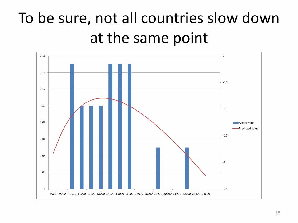
To be sure, not all countries slow down at the same point

18

Importantly, however, the right tail is made up of very small economies (not so reassuring…)

19

What increases the likelihood of a slowdown sooner rather than later?

• Answer: three factors: – Increasingly unfavorable demography.

• Sounds like China.

• Population aged 15-24 will fall by 21% over the next decade.

– Very high investment rate. • Sounds like China.

– Undervalued currency. • Sounds like China.

20

What lies behind the demography result?

• Higher share of the elderly in the population means that you can’t grow simply by increasing the share of the population working.

• Elderly require more public spending on social services (health care and the like).

• Savings rates will be lower, other things equal. • Slower labor force growth will mean more upward

pressure on wages. – All these factors will operate with a vengeance in China

owing to its long-standing One Child Policy. • At the same time, cases like Germany suggest that, while a

growing demographic burden makes a slowdown more likely, it by no means makes it unavoidable.

21

What explains investment result?

• Quite simply, no country can invest 50 per cent of its GDP, as China does currently, productively for an extended period.

• We have all heard the tales of ghost towns, idle airports, empty bullet trains, excess capacity in cement, aluminum, steel, auto parts.

• A high investment supports growth now but causes financial vulnerabilities to build up.

• It also creates a façade of prosperity, allowing the authorities to put off needed reforms.

22

What explains undervaluation result?

• A cheap (“undervalued”) currency is good for promoting the growth of unskilled labor-intensive manufacturing.

• But this same reliance on cheap labor weakens the pressure to move up the ladder into the production of more technologically sophisticated products.

• Eventually the pool of cheap rural labor is drained, and other even cheaper-labor countries come along.

• Hence undervaluation can boost growth for a time but becomes a liability as a country approaches Chinese levels of per capita income.

23

The conclusion follows that a growth slowdown is coming, but not tomorrow

• Growth is likely to step down by 3.5 percentage points or

more between 2003-10 and 2011-18 if the experience of other countries and my analysis is any guide.

• Consistent with this, at the most recent People’s Congress, which concluded in March, Chinese leaders suggested that growth would average on 7.5% this coming year.

• But, if so, a further slowdown to levels lower than 7.5% will likely be coming subsequently.

• The only question is whether this slowdown will be smooth and gradual or disruptive and abrupt. – In January I said “stay tuned.” – So what does the recent evidence suggest?

24

But an immediate slowdown?

• The picture is murky.

• Housing prices in the 100 largest cities (at upper right) continue to fall.

• Export growth (at lower right) is slowing.

25

But an immediate slowdown?

• But consumer confidence (upper right) continues to recover, weak housing prices notwithstanding.

• And the authorities still have plenty of policy levers to pull (bank loans continue to grow at a 15 per cent annual pace, as seen at right).

26

And if that isn’t confusing enough • While the latest official

purchasing managers’ survey (at right) points to strong growth in March, HSBC’s alternative was weak (48.3).

• While industrial production has been rising, inventories have been rising faster.

• While consumer confidence has been rising, retail sales growth has been slowing.

• Data released 10 days ago showed that China grew by 8.1% in 2012 Q1 (below consensus). But these numbers are subject substantial revision. – Murky is the word…. 27

David Card, in his lecture, asked the following questions about immigration

28

29

30

While immigrants have lower educational attainment, this is mainly

associated with Hispanics

31

And immigrants clearly like California

32

Why this geographic pattern?

33

You can see this here

34

35

36

And what are the effects of immigration? Do more immigrants cause lower wages for low skilled natives? Not obviously

37

38

Questions about methodology

• Immigrants don’t arrive randomly.

• Maybe the flow to cities where wages for unskilled natives are high.

• In this case, even if they drive down wages, ceteris paribus, we would not see effects.

• So look for a natural experiment.

• That’s why Card looks at the Mariel Boatlift…

39

John Morgan on Online Markets

• John inquired into the efficiency of these markets.

• And if there are anomalies, what accounts for them?

• Why can multiple on line auction sites coexist when thickness externalities matter?

• Many results in the presentation; this evening I will mention only a few.

40

Are prices necessarily driven to equality?

41

Answer is no: Price dispersion is considerable and persistent

42

But market structure matters (The more sellers, the less price dispersion –

reassuringly to economists, competition does appear to help)

43

Why this persistent price dispersion?

• It could be that sellers are trying to achieve two goals at the same time: to sell to “loyal customers” who will buy even at a high price, and to comparison shoppers who are very sensitive to prices.

• We thus may be seeing “hit and run” pricing where prices are cut sharply on occasion to attract comparison shoppers, who are continuously surfing but otherwise kept high to extract surplus from loyal customers.

• This is a more complicated pricing strategy than described in the textbooks. It’s an example of how modeling the behavior of sellers can be importantly informed by real world observation (in this case, of internet markets).

44

John finds suggestive evidence of this when comparing products

• In a study of computer memory chips, he finds that highly elastic (he estimates elasticities of -25 to -40). Evidently, first do not mark up prices to near-monopoly levels.

• In a study of Amazon’s book sales, in contrast, he finds that demand is inelastic (he estimates elasticities of -0.6). The firm has marked up prices to the inelastic range, where lowering the price by $1 gains you less than one additional volume of sales.

45

So why this difference?

• Books are sold on line: – In a concentrated market

– With heavy branding activity

– Direct sales

– Repeat customers • These are the “loyal customers”

• Computer memory is sold on line: – In a fragmented market

– With little branding by retailers

– There exist comparison site sales

– Consumers are sophisticated • These are the “comparison shoppers” who are surfing all the time.

46

Next question: why hidden fees?

47

Statement of hypothesis: This kind of pricing is efficient

48

Alternative hypothesis: It allows firm to shroud prices from naïve consumers

• Thereby transferring a larger portion of the market prices to shipping fees or baggage fees (that are not advertised as part of the headline price) increases revenue.

• Even when there are many sellers, market competition does not eliminate this so-called framing effect. – Some support in the data, as we saw, for both

interpretations.

49

Finally, do more efficient platforms outcompete less efficient ones?

• Famous hypothesis: in network markets, the first mover prevails whether more efficient or not.

• QWERTY keyboard vs. Dvorak Simplified keyboard.

• But there is also an alternative telling of the story.

50

When we speak of platforms, what do we mean?

51

Consider following experimental design

• John’s experiment assumes that 2 platforms have the same match technology (same payoffs).

• But platforms differ in their access fees (so there is a Pareto ranking of which platform yields the most surplus to consumers). – Note that this is a good example of how well designed

laboratory experiments can be used to ask and answer important economic questions.

– But, as with any experiment, having a well-designed experimental setting is key.

52

Seems like the cheaper platform prevails even if it lacks first-mover advantage

53

Same result obtains when the platform with higher user fee also delivers better matches and therefore should prevail: it prevails even if it starts out behind

54

• There is no support here for QWERTY.

– The (Pareto) inferior platform wins 0% of time.

• There is no evidence of expectational lock-in.

– First mover has no enduring advantage.

• Surplus is what matters.

– Platform offering the higher surplus triumphs 100% of the time.

55

Next we had Fred Finan on corruption

• Causes and effects of corruption may not seem like a mainstream economic question.

• But, to the contrary, it is a prime example of the kind of new questions to which economists have increasingly turned.

• Why? Because of evidence (and the presumption) that corruption is bad for economic growth.

56

57

But this kind of evidence has limits

• Illicit nature of corruption makes it hard to measure accurately.

• Aggregate measures (from NGOs Transparency International) are arbitrary and less than convincing.

• They are based on surveys of, inter alia, investors, whose opinions are often subjective.

• Corruption measures are correlated with other country characteristics.

• This creates an evaluation problem (what is the counterfactual?).

• Even “natural experiments” like corruption crackdowns are not always natural (their imposition is targeted where corruption is the worst…?).

58

Indeed, some arguments suggest that corruption is not all that bad

• The surplus (what the driver gains from obtaining a license) may simply go to the bureaucrat instead of the public coffers (just redistribution, no inefficiency).

• Theory of the second best: in an overregulated system, bribes to get around regulation may actually improve efficiency (people need licenses, and bribes are an efficient way of getting them).

59

Research solution: randomization

• Bretrand and her coauthors randomly assigned Indian driver’s license applicants to 2 groups:

• This is a slight simplification of what they actually do…

– Group 1: People who were offered a financial reward (a bonus) if they obtained their license fast.

– Group 2: A control group offered nothing. • The control group illustrates extent of corruption: 71 per cent of

those obtaining a license avoided the mandated driving test. Those in the control group also pay more than twice the official fee (bribe).

• Bonuses increase the prevalence of bribes (suggesting that corruption may simply “grease the wheels” – that they are a response to incentives. But they also result in more incompetent licensed drivers, suggesting that bribes may be inefficient.

60

Second solution: use natural experiments like when Brazilian municipalities cracked

down on corruption

• Authors’ question: does greater transparency about discourage corruption?

• And, if so, through what channels?

• Specifically, does disclosing local government corruption practices reduce mayors’ probability of reelection?

61

• As Fred notes, the previous literature could say little about such questions because: – A) Information about corruption was nonrandom

– B) Corruption was poorly measured. • In Finan’s data, in contrast, municipalities were

randomly selected for audits of how they used federal funds/grants (some audits were before elections, some after). Each month 60 municipalities were randomly selected for audits. Audits were rigorous (measures of corruption were rigorous). And results were widely disseminated by media.

62

• Measure of corruption in this study: – Number of irregularities associated with, inter alia,

fraud in procurement, diversion of public resources, over-invoicing.

• Result: – One violation reduced reelection probability by 5%.

Three violations reduced it by 17%.

• This is clear evidence that public cares about corruption: – That the grease-in-the-wheels story is at best a minor

part of what is going on.

63

David Romer: Monetary Policy at the Zero Lower Bound

• How to think about it?

• How much does it matter?

• Policies to address the problem

64

• The standard framework.

• Starts with the IS curve: lowering interest rates makes borrowing less expensive, stimulates spending, resulting in higher income.

65

• Superimpose the MP (monetary policy curve): a standard central bank reaction function makes the interest rate r rise with inflation ᴨ and output y.

• Note that we are holding ᴨ constant for purposes of constructing the diagram (you can only show the relationship between 2 variables in two-dimensional space…)

66

• What is the effect of lowering the expected rate of inflation in this model (as in lower quadrant)?

• Answer: the central bank will lower the r that corresponds to any y (MP schedule shifts down in upper quadrant).

67

• But the nominal interest rate can’t be less than 0.

• Meaning that the real interest rate on which spending depends will be stuck at (0-ᴨ) if expected inflation is stuck at ᴨ. – (Everyone should be sure

they understand the definition and meaning of “nominal” and “real” interest rate.)

68

• This also means that if output falls the normal stabilizing impact of interest rate cuts will be missing.

• As now. We would have a -4% federal funds rate now if we could, given prevailing levels of output and inflation.

69

What can be done about this?

• You want to reduce the real interest rate (0-ᴨ) on which spending depends.

• You can do this by raising ᴨ. • How to accomplish this?

– Expand the central bank’s balance sheet (QE) to raise expected future inflation.

– Use communications policy (use open mouth operations), and through that channel raise expected future inflation.

– Create expectations of currency depreciation (create expected import-price inflation).

70

• So has the zero lower bound been a problem in practice?

• And, if so, how has that problem been solved?

– David pointed to three instances where it has been a problem in practice:

• US in 1930s

• Japan in 1990s

• US in 2010s

71

Japan in 1990s

• Interest rates were certainly close to zero (see right).

• How were they dealt with?

• Answer: ineffectively. – BOJ was slow to act.

– Communications policy was ineffective (the central bank sent mixed messages).

– Afraid to create inflationary expectations.

– Afraid to depreciate the yen.

– Is now different? (We shall see.)

72

US in 1930s

• Interest rates were close to zero (see right).

• Nothing was done until 1933. But then: – Roosevelt took the US off

the dollar (communicating that there was a new regime).

– He depreciated the exchange rate.

– This transformed expectations (real interest rates fall sharply starting in 1933).

73

US in 2010s

• Interest rates are clearly near zero.

• Fed is trying to generate expected inflation.

• How: – Quantitative easing to

create expectations of higher future inflation.

– Forward guidance committing to future policy.

– Communications policy in general.

74

But has the Fed been too tentative?

• Too worried about creating inflationary expectations when that is exactly what we need at the zero lower bound.

• Reluctant to pursue QE on a larger scale, when that is exactly what we need to create inflationary expectations.

• Reluctance to depreciate the exchange rate. – For reasons Brad DeLong emphasized.

• Unwilling to make unconditional policy commitments about keeping interest rates low for an extended period (Fed’s language in its statements is conditional, which doesn’t help). – Why this reluctance, one might ask? Political pressure?

75

76

• Brad DeLong covered many of these same issues.

• In addition, he discussed the role of fiscal policy in an environment of near zero interest rates.

77

A core argument is that fiscal policy has a larger impact when interest rates

are at the zero lower bound

• The intuition is pretty clear. • Shifting the IS curve to the right

(through spending increases or tax cuts should have an even bigger impact when the MP curve is horizontal than otherwise).

• Think of it this way (following DeLong): in normal circumstances, the Fed offsets the impact of any fiscal-policy impulse on the level of output (since it is already at a desirable output-interest rate combination). But at the zero lower bound, it does not.

78

• This also points us to the more general point that the effects of fiscal policy (of shifting the IS curve) depend on the monetary policy response (the Fed can control, presumably, the steepness of the upward-sloping portion of the MP curve).

79

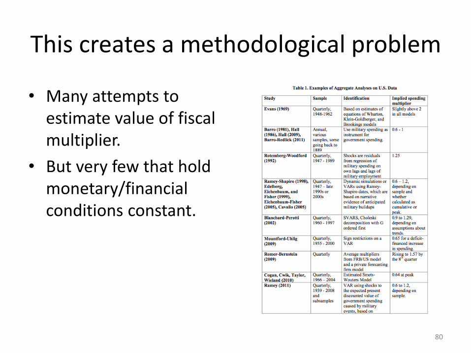
This creates a methodological problem

• Many attempts to estimate value of fiscal multiplier.

• But very few that hold monetary/financial conditions constant.

80

• I would observe that there is at least one attempt to do this.

• Almuna, Benetrix, Eichengreen, O’Rourke and Rua, Economic Policy (2010).

• And we get a multiplier of approximately two.

• How we do it (we control separately for the stance of monetary policy and use an instrument for fiscal expansion…)

81

• The problem today being, as Brad noted, that not everyone has the same, or adequate, fiscal room for maneuver.

82

• Bottom line: good research in economics (as in any empirical discipline) requires: – Clearly-stated question

– Explanation of why it’s important

– A clear methodology/set-up for addressing it

– Detailed data

– Careful though on relating theory to analysis of the data

• And that is what you should aspire to achieve in your research paper.

83