richard holden - econstor.eu
TRANSCRIPT
econstorMake Your Publications Visible.
A Service of
zbwLeibniz-InformationszentrumWirtschaftLeibniz Information Centrefor Economics
Aghion, Philippe; Fehr, Ernst; Holden, Richard; Wilkening, Tom
Working Paper
The Role of Bounded Rationality and ImperfectInformation in Subgame Perfect Implementation: AnEmpirical Investigation
IZA Discussion Papers, No. 8971
Provided in Cooperation with:IZA – Institute of Labor Economics
Suggested Citation: Aghion, Philippe; Fehr, Ernst; Holden, Richard; Wilkening, Tom (2015) : TheRole of Bounded Rationality and Imperfect Information in Subgame Perfect Implementation: AnEmpirical Investigation, IZA Discussion Papers, No. 8971, Institute for the Study of Labor (IZA),Bonn
This Version is available at:http://hdl.handle.net/10419/110701
Standard-Nutzungsbedingungen:
Die Dokumente auf EconStor dürfen zu eigenen wissenschaftlichenZwecken und zum Privatgebrauch gespeichert und kopiert werden.
Sie dürfen die Dokumente nicht für öffentliche oder kommerzielleZwecke vervielfältigen, öffentlich ausstellen, öffentlich zugänglichmachen, vertreiben oder anderweitig nutzen.
Sofern die Verfasser die Dokumente unter Open-Content-Lizenzen(insbesondere CC-Lizenzen) zur Verfügung gestellt haben sollten,gelten abweichend von diesen Nutzungsbedingungen die in der dortgenannten Lizenz gewährten Nutzungsrechte.
Terms of use:
Documents in EconStor may be saved and copied for yourpersonal and scholarly purposes.
You are not to copy documents for public or commercialpurposes, to exhibit the documents publicly, to make thempublicly available on the internet, or to distribute or otherwiseuse the documents in public.
If the documents have been made available under an OpenContent Licence (especially Creative Commons Licences), youmay exercise further usage rights as specified in the indicatedlicence.
www.econstor.eu

DI
SC
US
SI
ON
P
AP
ER
S
ER
IE
S
Forschungsinstitut zur Zukunft der ArbeitInstitute for the Study of Labor
The Role of Bounded Rationality and Imperfect Information in Subgame Perfect Implementation: An Empirical Investigation
IZA DP No. 8971
April 2015
Philippe AghionErnst FehrRichard HoldenTom Wilkening
The Role of Bounded Rationality and Imperfect Information in Subgame Perfect
Implementation: An Empirical Investigation
Philippe Aghion Harvard University, CEPR and NBER
Ernst Fehr
University of Zurich and IZA
Richard Holden University of New South Wales
Tom Wilkening University of Melbourne
Discussion Paper No. 8971 April 2015
IZA
P.O. Box 7240 53072 Bonn
Germany
Phone: +49-228-3894-0 Fax: +49-228-3894-180
E-mail: [email protected]
Any opinions expressed here are those of the author(s) and not those of IZA. Research published in this series may include views on policy, but the institute itself takes no institutional policy positions. The IZA research network is committed to the IZA Guiding Principles of Research Integrity. The Institute for the Study of Labor (IZA) in Bonn is a local and virtual international research center and a place of communication between science, politics and business. IZA is an independent nonprofit organization supported by Deutsche Post Foundation. The center is associated with the University of Bonn and offers a stimulating research environment through its international network, workshops and conferences, data service, project support, research visits and doctoral program. IZA engages in (i) original and internationally competitive research in all fields of labor economics, (ii) development of policy concepts, and (iii) dissemination of research results and concepts to the interested public. IZA Discussion Papers often represent preliminary work and are circulated to encourage discussion. Citation of such a paper should account for its provisional character. A revised version may be available directly from the author.
IZA Discussion Paper No. 8971 April 2015
ABSTRACT
The Role of Bounded Rationality and Imperfect Information in Subgame Perfect Implementation: An Empirical Investigation* In this paper we conduct a laboratory experiment to test the extent to which Moore and Repullo’s subgame perfect implementation mechanism induces truth-telling in practice, both in a setting with perfect information and in a setting where buyers and sellers face a small amount of uncertainty regarding the good’s value. We find that Moore-Repullo mechanisms fail to implement truth-telling in a substantial number of cases even under perfect information about the valuation of the good. This failure to implement truth-telling is due to beliefs about the irrationality of one’s trading partner. Therefore, although the mechanism should – in theory – provide incentives for truth-telling, many buyers in fact believe that they can increase their expected monetary payoff by lying. The deviations from truth-telling become significantly more frequent and more persistent when agents face small amounts of uncertainty regarding the good’s value. Our results thus suggest that both beliefs about irrational play and small amounts of uncertainty about valuations may constitute important reasons for the absence of Moore-Repullo mechanisms in practice. JEL Classification: D23, D71, D86, C92 Keywords: implementation theory, incomplete contracts, experiments Corresponding author: Ernst Fehr Department of Economics University of Zurich Bluemlisalpstrasse 10 CH-8006 Zurich Switzerland E-mail: [email protected]
* We owe special thanks to Michael Powell and Eric Maskin. We also thank Christopher Engel, Oliver Hart, Martin Hellwig, Andy Postlewaite, Klaus Schmidt, Larry Samuelson, and seminar participants at the 2010 Asian-Pacific ESA Conference (Melbourne, Australia), Bocconi, Chicago Booth, Harvard, MIT, Stanford, the IIES in Stockholm, the Max Planck Institute in Bonn, UNSW and University of Queensland for helpful comments. We gratefully acknowledge the financial support of the Australian Research Council including ARC Future Fellowship FT130101159 (Holden) and ARC Discovery Early Career Research Award DE140101014 (Wilkening), the University of Melbourne Faculty of Business and Economics, and the European Research Council grant on the Foundations of Economic Preferences (Fehr).
1 Introduction
Subgame Perfect Implementation has attracted much attention since it was introduced by
Moore & Repullo (1988). A main reason for this success is the remarkable property that
almost any social choice function can be implemented as the unique subgame perfect equi-
librium of a suitably designed dynamic mechanism.1 This was perceived as a substantial
improvement over Nash implementation, which suffered from two main limitations: first, it
would allow only a certain class of social choice rules to be implemented, those which are
“Maskin Monotonic” (Maskin, 1977; Maskin, 1999); roughly speaking, Nash implementation
does not permit the implementation of social choice rules that involve distributional concerns
between the agents. Second, Nash implementation typically involves multiple equilibria, so
that even if a desirable equilibrium exists, an undesirable one may too.2
A common objection to subgame perfect implementation mechanisms, however, is that
they are hardly observed in practice. This in turn raises the question as to why one does
not observe them. A first type of answer, developed by Fudenberg, Kreps & Levine (1988),
is that the behavioral assumptions embedded in subgame perfection may not be a good
approximation of actual behavior. Another type of answer, recently put forward by Aghion,
Fudenberg, Holden, Kunimoto & Tercieux (2012), henceforth AFHKT, is that subgame
perfect implementation is not robust to arbitrarily small deviations from common knowledge.
In this paper we use a laboratory experiment to test the extent to which the Moore-
Repullo mechanism implements truth-telling in practice, both in a setting with perfect in-
formation and in a setting where buyers and sellers do not share common knowledge about
the good’s valuations. We implement three treatments: one with perfect information about
the value of the good (we refer to it as the no-noise treatment); one with 5% imperfect in-
formation (i.e., traders receive information about the good’s valuation that is 95% correct);
and one with 10% imperfect information (traders have information that is 90% correct). We
also conducted a robustness check with only 1% imperfect information to examine whether
even very small deviations from complete information can cause serious failures in inducing
truth-telling.
Our environment is taken from Hart & Moore (2003) where a seller is about to receive a
buyer-specific good of either high or low quality. Before learning the value of the good, the
buyer and seller would like to write a contract where the buyer pays a high price if the good
1Subgame perfect implementation also assumes that individuals are sequentially rational and that transfersof any size are allowed.
2Uniqueness can be obtained through the use of so-called “integer games” whereby parties simultaneouslyannounce an integer and the player with the largest announcement has her preferred option implemented.These have been widely criticized, particularly since the infinite strategy means that best responses are notwell-defined (Jackson 1992), and for being unimportant in practice.
2
is of high quality and a low price if the good is of low quality. However, the quality of the
good is not verifiable by a third-party court and thus a state-dependent contract cannot be
directly enforced.
While the state is not verifiable, public announcements can be recorded and used in legal
proceedings. Thus the two parties can in principle write a contract that specifies trade prices
as a function of announcements made by the buyer. If the buyer always tells the truth, then
his announcement can be used to set state-dependent prices. One way of doing this is to
implement a mechanism that allows announcements to be challenged by the seller and to
punish the buyer any time he is challenged. If the seller challenges only when the buyer has
told a lie, then the threat of punishment will ensure truth-telling.
The key challenge of developing the implementation mechanism is to construct a set of
actions such that the seller has an incentive to challenge lies but to prevent the seller from
challenging the buyer when he has in fact told the truth. The SPI mechanism we consider
accomplishes this by having a sellers challenge trigger two actions: a punishment, in the
form of a fine, and a counter-offer. This counter-offer is structured so that if the buyer was
lying he will accept the counter-offer and if he was telling the truth he will reject it. By
conditioning additional award and punishments to the seller based on whether the counter-
offer was accepted or rejected, the mechanism can prevent sellers from abusing their power
by challenging when the buyer had indeed told the truth.
For the SPI mechanism to induce truth-telling, it must be structured so that (i) buyers
have an incentive to accept counter-offers after a lie and to reject counter-offers after the truth
and (ii) sellers have an incentive to challenge lies and not challenge truthful announcements.
When experimenting with the SPI mechanism outlined above under full information, we find
that the mechanism is very successful in inducing these behaviors. In line with what the
theory would predict, buyers always reject counter-offers after a truthful announcement and
accept counter-offers over 90% of the time after a lie; sellers challenge lies over 90% of time
and challenge truthful announcements in less than 5% of cases.
Surprisingly, however, the mechanism in our full information treatment fails to induce
truth-telling in a substantial number of cases. Despite correct pecuniary incentives, buyers
who observe a high quality good lie over 30% of the time and about 10% of buyers lie in
every period. Based on beliefs data, these lies appear to be due to buyers who are pessimistic
about the rationality of the sellers and fear that truthful announcements will be challenged.
To better understand the extent to which beliefs are playing a role, we ran an additional
treatment where we elicit incentive compatible beliefs using a mechanism developed by Karni
(2009). We find that not only do the majority of individuals who lie believe that they have
a higher expected pecuniary payoff for lying than for telling the truth, but the majority of
3
individuals who tell the truth also hold these beliefs. This finding is due primarily to a large
majority of buyers who believe that truth-telling may be challenged. Thus paradoxically,
while the mechanism is designed to induce truth-telling based on pecuniary incentives, the
mechanism is in fact associated with beliefs that render lying profitable for the buyers —
even for the majority of buyers who tell the truth. Thus, it appears that a substantial
amount of the observed truth-telling is not due to the mechanism but to the buyers’ intrinsic
preferences for honesty.
Next, we analyze how the SPI mechanism performs in the presence of imperfect informa-
tion. More specifically, we introduce two noise treatments where we give buyers and sellers
imperfect signals about the underlying quality of the good which are correct either 90% or
95% of the time. According to AFHKT the introduction of noise should induce buyers to
believe that lying, i.e., the announcement of a low value after a high signal, is less likely to be
challenged by the sellers. For this reason, the buyers are also predicted to increase their rate
of lying. We find that these predictions are well supported in the data. The introduction of
noise increases the proportion of buyers who announce a low value with a high signal by 15
to 25 percentage points relative to the no-noise treatment. These buyer lies are persistent in
the noise treatment and do not diminish with experience. Further, the introduction of noise
causes a significant change in buyers’ beliefs; they are now much more likely to believe that
lying will not be challenged. In addition to the patterns predicted by AFHKT, we observe
that the introduction of noise also exacerbates a pattern that we already observed in the
perfect information treatment: the buyers have even more pessimistic beliefs about being
challenged after truth-telling although — according to the theory — truthful announcements
should never be challenged.
In a further experiment, we study how the introduction of even small amounts of noise
impacts the mechanism. In a treatment where individuals are given the correct signal 99%
of the time, we find that the introduction of noise increases buyer lies to the levels observed
in the 95% noise treatment. Thus, even very small deviations from common knowledge can
have a big effect on the outcome of the mechanism.
The buyers’ beliefs that even truthful announcements will be challenged by the sellers
seems to play an important role for the mechanism’s failure to induce truth-telling both
under complete and incomplete information. But does this belief indeed cause buyers’ lies?
To examine this question, we also study what Moore (1992) refers to as a simple mechanism
where we prevent buyers from being challenged if they announce a high valuation for the
good. This simple mechanism can implement the first best in our setting but would not
function in more complicated environments where both parties must announce truthfully.
In a treatment of this mechanism with no noise, the new mechanism dramatically reduces
4
the proportion of buyer lies, providing direct evidence that strategic uncertainty is driving
most of the lies in the no-noise treatments. With noise, however, buyer lies continue to be
common. Overall, our findings suggest that small amounts of private information do indeed
lead to large deviations from truth-telling and significantly more lies than under perfect
information.
This paper relates to several strands of literature. It first contributes to the literature on
mechanism design and more specifically on subgame perfect implementation (Maskin, 1999;
Moore & Repullo, 1988; Maskin & Tirole, 1999a; Chung & Ely, 2003) by pointing to two
main sources for the failure of SPI mechanisms: namely, players’ beliefs about the possibility
of irrational challenges by other players, and (small) deviations from common knowledge. In
particular we show that beliefs about the irrationality of the trading partner undermine the
SPI mechanism even in the case of perfect information about the good’s value. This in turn
suggests that future work should concentrate on the design and examination of mechanisms
that are robust to deviations from perfect information and perfect rationality.3 Our results
also point to a preference for truth-telling that causes some individuals to go against their
belief-based pecuniary payoffs and make truthful announcements. This result suggests that
it may be possible to design more efficient implementation mechanisms that utilize these
preferences for honesty.4
Second, our paper contributes to the debate on the foundations of incomplete contracts.
In their influential 1986 paper, Grossman and Hart argued that in contracting situations
where states of nature are observable but not verifiable, asset ownership (or vertical in-
tegration) can help limit ex post hold-up and thereby encourage ex-ante investments (see
Grossman & Hart (1986)). However, in subsequent work, Maskin & Tirole (1999a, 1999b)
used subgame perfect implementation to show that the non-verifiability of states of nature
can be overcome using a 3-stage subgame perfect implementation mechanism which induces
truth-telling by all parties as the unique equilibrium outcome. Our paper sheds light on
why such mechanisms are not observed in practice, which in turn helps explain why vertical
integration or control allocation matter.
Finally, our paper also contributes to the experimental literature on implementation.
Sefton & Yavas (1996) study extensive-form Abreu-Matsushima mechanisms that vary in
the number of stages used and find that incentive-compatible mechanisms with 8 and 12
stages perform worse than a mechanism with 4 stages that is not incentive compatible.
3The systematic under estimation of the rationality of others is similar to results in Huck & Weizsacker(2002) who find that beliefs about the play of others are distorted towards the uniform prior.
4Our result that many individuals tell the truth when their monetary gain from truth-telling is negative isrelated to the literature on lying aversion (Gneezy, 2005; Sanchez-Pages & Vorsatz, 2007; Ederer & Fehr,2009).
5
Katok, Sefton & Yavas (2002) study both simultaneous and sequential versions of the Abreu-
Matsushima mechanism and conclude that individuals use only a limited number of iterations
of dominance and steps of backward induction. Based on these papers, we limited out
attention to mechanisms that require only two levels of backward induction.5 Fehr, Powell, &
Wilkening (2014) study a related subgame-perfect implementation mechanism in the context
of a hold-up problem. They find that reciprocity and other-regarding preferences cause the
SPI mechanism to fail: The mechanism often does not solve the hold-up problem and the
trading parties have generally higher pecuniary returns in the absence of the mechanism such
that they refuse to enter the mechanism in the majority of the cases. In the current paper
we intentionally designed our mechanism and environment in such a way that reciprocity
was unlikely to play a role.6 Therefore, we could concentrate on how imperfect information
and other forces such as irrational beliefs and strategic uncertainty affect the performance
of the mechanism. Our results show that these forces strongly impair the functioning of the
mechanism.
The remaining part of the paper is organized as follows. Section 2 presents the sim-
ple model which guides our experimental design. Section 3 describes the experiment and
hypotheses. Section 4 presents the experimental results under perfect and imperfect infor-
mation. Section 5 concludes by suggesting broader implications from our experiment and
avenues for future research.
2 Theoretical Motivation
In this section we present a simple example which will guide our experimental design.
2.1 Common Knowledge
The following example is a slight modification of one used in AFHKT, and based on Hart
& Moore (2003).7 There are two parties, a B(uyer) and a S(eller) of a single unit of an
5An extensive experimental literature also exists looking at efficiency of implementation mechanisms in thepublic goods provision problem. Chen & Plott (1996), Chen & Tang (1998), and Healy (2006) studylearning dynamics in public good provision mechanisms. Andreoni & Varian (1999) and Falkinger, Fehr,Gachter, & Winter-Ebmer (2000) study two-stage compensation mechanisms that build on work fromMoore-Repullo (1988), while Harstad & Marese (1981, 1982), Attiyeh, Franciosi, & Isaac (2000), Arifovic& Ledyard (2004), and Bracht, Figuieres, & Ratto (2008) study the voluntary contribution game, Groves–Ledyard, and Falkinger mechanisms respectively. Masuda, Okano & Saijo (2014) study approval mechanismsand emphasize the need for implementation mechanisms to be robust to multiple reasoning processes andbehavioral assumptions.
6We deliberately chose parameters in our experiment that made reciprocal behavior very costly and thusvery unlikely to occur. We show this more explicitly in Section 3.3.1.
7The original example is also reported in Aghion & Holden (2011).
6
indivisible good. If trade occurs then B’s payoff is VB = θ − p, where θ is the value of the
good and p is the price. S’s payoff is just VS = p.
The good can be of either high (the state is θ = θH) or low quality (θ = θL). If it is
high quality then B values it at 70, and if it is low quality then B values it at 20. Before θ
is realized both parties would prefer to trade at a price p(θ) = θ2. This price always ensures
that trade occurs when it is efficient and splits the surplus evenly between the buyer and
the seller in all states of the world so that inequity aversion does not influence the desire for
trade.
The value θ is observable and common knowledge to both parties but non-verifiable by
a court. The assumption that the value θ is non-verifiable implies that no contract can be
written that is credibly contingent on θ. However, truthful revelation of θ can be achieved
through the following Moore-Repullo (MR) mechanism which can indirectly generate the
desired price schedule:
1. B announces either “high” or “low”. If “high” and S does not “challenge” B’s an-
nouncement, then B pays S a price equal to 35 and the game then ends.
2. If B announces “low” and S does not “challenge” B’s announcement, then B pays a
price equal to 10 and the game ends.
3. If S challenges B’s announcement then:
(a) B pays a fine of F = 25 to T (a third party).
(b) B is made a counter-offer for the good at a price of 75 if his announcement was
“high” and a price of 25 if his announcement was “low.”
(c) If B accepts the counter-offer then S receives the fine F = 25 from T (and also
the counter-offer price from B) and the game ends.
(d) If B rejects the counter-offer then S pays F = 25 to T . S also gives the good to
T who destroys it and the game ends.
When the true value of the good is common knowledge between B and S this mechanism
yields truth-telling as the unique subgame-perfect equilibrium. The logic of this equilibrium
is that the initial-prices, counter-offer prices, and fines are constructed so that if B and S are
commonly known to be sequentially rational, B only has an incentive to announce “high” if
θ = θH and “low” if θ = θL. For this to be true, the mechanism must satisfy three conditions.
(i) Counter-Offer Condition. B must prefer to accept any counter-offer for which he
has announced “low” when θ = θH . B must prefer to reject any counter-offer for which
he has announced “low” when θ = θL or for which he announced “high”.
7
(ii) Appropriate-Challenge Condition. S must prefer to challenge an announcements
of “low” when θ = θH and must prefer not to challenge an announcement of “low”
when θ = θL. S must prefer to never challenge “high”.
(iii) Truth-Telling Condition. B must prefer to announce “low” if θ = θL and “high” if
θ = θH .
We refer to challenging “low” when θ = θH as an appropriate challenge. The Counter-
Offer Condition requires that after an appropriate challenge, the counter-offer price is below
the value of the good so that B has a pecuniary incentive to accept the counter-offer. Since the
counter-offer price after “low” is 25, this requirement is met. The Counter-Offer Condition
also requires that after any other challenge, the counter-offer price is above the value of the
good so that B has a pecuniary interest to reject the counter-offer. Since the counter-offer
prices for “low” is 25 and the counter-offer price for “high” is 75, this second requirement is
met.
As prices and counter-offers are constructed to satisfy the Counter-Offer Condition, B
will reject counter-offers following inappropriate challenges and will accept counter-offers fol-
lowing appropriate challenges. This implies the Appropriate-Challenge Condition is satisfied
if S has an incentive to challenge only in cases when B will accept such a challenge (i.e.,
when B announces “low” when θ = θH). This condition is satisfied since the counter-offer
price of challenging a “low” announcement (25) plus the fine (25) exceeds the price that
occurs if the announcement is not challenged (10).
Finally, for the Truth-Telling Condition to be satisfied, B must prefer to announce “low”
if θ = θL and “high” if θ = θH . Since the price paid by announcing “high” is higher than the
price paid by announcing “low” and an appropriate challenge never occurs when θ = θL, B
never has an incentive to overreport his value by announcing “high” when θ = θL. Further,
B will always be challenged for announcing “low” when θ = θH . Adding the counter-offer
price and the fine, a buyer’s total payment if he lies by announcing “low” when θ = θH is
50. As the price paid for announcing “high” is 35 and lower than the total payments from
lying, B has no incentive to underreport and announces truthfully when θ = θH as well.
Thus the above mechanism yields unique implementation in subgame perfect equilibrium.
That is, for any realization of θ, there is a unique subgame perfect equilibrium which yields
different prices for different valuations of the good. Moreover, in each state, the unique
subgame perfect equilibrium is appealing from a behavioral point of view since it consists of
telling the truth and it splits the surplus equally among B and S. Both of these properties
fail once we introduce small common p-belief perturbations.
8
2.2 The Failure of Truth-Telling Under (Small) Informational Per-
turbations
We now introduce a small common p-belief perturbation from common knowledge about the
valuation θ. We assume (i) the players have a common prior µ, (ii) µ(θ = θH = 70) = .5,
and (iii) µ(θ = θL = 20) = .5.8 Each player receives an independent draw from a signal
structure with two possible signals: sH or sL, where sH is a high signal where θ equals 70
with probability 1− ε, and sL is a low signal where θ is equal to 20 with probability 1− ε.We use the notation sHB (resp. sLB) to indicate that B received the high signal sH (resp. the
low signal sL).
First, as in AFHKT, we can show that there is no equilibrium in pure strategies in
which the buyer and seller always report truthfully. To see this, suppose instead that such
an equilibrium exists, and further suppose that B gets signal sLB, announces “low,” and is
challenged. Under a truth-telling equilibrium, the buyer’s belief is that his signal and the
seller’s signal are incorrect with equal probability, and thus the expected value of the good
is 45. As this is above the counter-offer price of 25, the buyer has an incentive to purchase
regardless of his signal.
Anticipating the acceptance of challenges with a low signal and “low” announcement, the
seller now has an incentive to challenge even if his signal is sLS . It follows that there does not
exist an equilibrium where all parties are truth-telling in pure strategies. For slight changes
in the environment, a similar pattern can hold in the case of a buyer who receives signal sHBand is considering whether to make the “high” or “low” announcement. In this case, under
the truth-telling equilibrium, the seller will be unsure as to the value of the good and may
not challenge the announcement if she believes the buyer will reject the counter-offer.9
AFHKT further show that when introducing even a small level of noise, the set of consis-
tent beliefs expands markedly, which gives rise to equilibria that involve a positive amount
8AFHTK consider a more general setting with an arbitrary prior. However, to map closest to the experiment,we develop the theoretical part with the same values, priors, and error distributions as those used in theactual experiment in the next section.
9These arguments extend to the limiting case where the value perturbations get very small. AFKHT showthat one can find a sequence of p-belief value perturbations parameterized by some noise variable ε, suchthat convergence to common knowledge corresponds to ε −→ 0, but truth-telling by the buyer (call itthe “good” equilibrium) is not approximately implementable as a mixed strategy sequential equilibrium ofthe above MR mechanism when ε −→ 0. They also show that one can find a sequence of p-belief valueperturbations parameterized by some noise variable ε and converging to common knowledge as ε −→ 0, suchthat the above MR mechanism under these perturbations admits a “bad” sequential equilibrium in whichthe probability of the buyer misreporting her signal remains bounded away from zero as ε −→ 0. Moregenerally, AFHKT show that, given any mechanism which “subgame-perfect” implements a non-monotonicsocial choice function f(θ), there always exists arbitrarily small common p-belief value perturbations underwhich a “bad” sequential equilibrium, whose outcome remains bounded away from f(θ) for at least onestate of nature θ, also exists.
9
of lies by buyers and/or false challenges by sellers. We consider particular deviations from
perfect information and derive the corresponding mixed strategy Perfect Bayesian Equilibria
(PBEs) in the experimental design section.
3 The Experiment
3.1 The Subgame-Perfect Implementation Game
At the center of our experimental design is a computerized version of the Subgame-Perfect
Implementation game we discussed in the previous section. In each of twenty periods, a buyer
is matched with a seller and randomly assigned one of two sealed containers.10 One container
is worth 70 ECU to the buyer while the other container is worth 20 ECU.11 Containers are
selected with equal probability and both the buyer and seller do not initially know which
container has been chosen while trading.
Each of the two containers is filled with red and blue balls whose composition changes
by treatment:
1. No-Noise Treatment: In the no-noise treatment, the container worth 70 ECU is
filled with 20 red balls and 0 blue balls. The container worth 20 ECU is filled with 20
blue balls and 0 red balls.
2. 5% Noise Treatment: In the 5% noise treatment, the container worth 70 ECU is
filled with 19 red balls and 1 blue ball. The container worth 20 ECU is filled with 19
blue balls and 1 red ball.
3. 10% Noise Treatment: In the 10% noise treatment, the container worth 70 ECU is
filled with 18 red balls and 2 blue balls. The container worth 20 ECU is filled with 18
blue balls and 2 red balls.
At the beginning of each period, one of the balls in the container assigned to the buyer is
randomly drawn and secretly shown to the seller. This ball is put back into the container and
a second ball is randomly drawn for the buyer but held privately to one side. These signals
provide perfect information regarding the container being traded in the no-noise treatment
10Subjects are randomly assigned the role of a buyer or of a seller and remain in this role throughout theexperiment.
11The experiment was conducted in experimental currency (ECU) and converted to Australian dollars at arate of 10 ECU = 1 AUD.
10
and almost perfect information in the 5% and 10% noise treatments.12
Before the buyer knows the color of his ball he is asked to make a public announcement
concerning the value of the container for the case in which the ball drawn for him is red
or blue. He may announce a value of either 70 ECU or 20 ECU in each of the two cases.
After making choices for both possible signals, the color of the ball drawn is revealed to him
and his declared strategy is implemented by the computer. This strategy method gives us a
complete set of announcement data in each period which precludes changes in the frequency
of lies over time due to random assignment of signals to different subsets of buyers. The
strategy method also allows for a complete panel of choices which improves our ability to
control for heterogeneity across individuals.13
The public announcement of the buyer is next seen by the seller as well as a computerized
arbitrator who acts as the implementation mechanism. After observing the announcement,
the seller has the option of accepting the announcement or calling the arbitrator. If the seller
accepts the announcement, trade occurs at a price equal to 1/2 of the announcement. If,
however, the seller elects to call the arbitrator, the buyer is immediately charged a fine of 25
ECU and the game continues on to the arbitration response stage.
In the arbitration response stage, the buyer is given a counter-offer by the computerized
arbitrator which is based on his initial announcement. If he announced a value of 70 ECU,
the arbitrator gives a counter-offer of 75 ECU. If he announced a value of 20 ECU, the
arbitrator gives a counter-offer of 25 ECU.
If the buyer accepts the counter-offer, trade occurs at the counter-offer price. In this
case the seller is given the 25 ECU which was previously charged as a fine to the buyer. If,
however, the buyer rejects the counter-offer, no trade occurs and the seller is also charged a
fine of 25 ECU yielding a loss of 25 ECU for both parties. Note that the structure of fines
ensures that under full information the subgame-perfect equilibrium is unique.14
In the event that trade occurs, the actual value of the container is revealed and the profits
of the buyer and seller are realized based on the value of the container, the price, and any
fines. The profits of each individual are calculated after each period.
In addition to action profiles of the implementation mechanism, we also elicited beliefs
12In the control quiz, subjects are asked to calculate the likelihood of the other party having the same colorball as them in each treatment. For the no-noise treatment we announce in the verbal summary that “ifyou see a red ball, you know with 100% certainty that your matched partner has also seen a red ball.Likewise, if you see a blue ball, you know with 100% certainty that your matched partner has also seena blue ball.” For the noise treatments we announce the probability that both parties observe the samesignal.
13We ran two pilot sessions without the strategy method. The lying rates in these pilot sessions were similarto those reported in the results section.
14The mechanism can also be made renegotiation proof by allowing for Nash bargaining in the case ofdisagreement and placing the fines in escrow so they cannot be recovered in cases of disagreement.
11

about the likelihood of actions of the other party. Likelihoods were recorded using a 4-point
likert scale (Never/Unlikely/Likely/Always). The belief elicitation was done in each period
directly after the buyer or seller took their action. For a buyer, we elicited the likelihood that
the seller would challenge an announcement of 20 ECU and 70 ECU in each period given his
observed signal, and we did so right after the buyer made her announcement decision but
before discovering the seller’s action. For a seller, we asked about his beliefs right after the
seller made his challenge decision. We asked each seller the likelihood that their challenge
would be rejected given their signal and the announcement of the buyer.
We did not pay subjects for their beliefs because in the main sessions we were primarily
interested in the behavioral data. If we had compensated subjects for both their beliefs
and their actions, risk averse subject could have found it optimal to hedge risk by stating
beliefs which differ from their true estimates - a possibility that is discussed in more detail
in Blanco, Engelmann, Koch & Normann (2010). Moreover, we ran four additional sessions
to check whether belief elicitation affects behavior. In these sessions subjects faced 5% noise
for 10 periods and then no noise for 10 periods. We find no behavioral differences between
these control sessions and the main sessions with the same treatment ordering and with
belief elicitation. In particular, the distribution of buyer announcements after a high signal
neither differs in the 5% noise treatments (Mann-Whitney-Wilcoxen test, p-value = .3930)
nor in the no-noise treatments (Mann-Whitney-Wilcoxen test, p-value = .3303).
3.2 Experimental Design and Protocols
Our experimental design utilizes a within-subjects design in which each subject is exposed
to 10 periods of the no-noise treatment and 10 periods of one of the two noise treatments.
A total of 16 sessions were run: eight with a 5% noise level and eight with a 10% noise
level. We conducted half the sessions starting with the no-noise treatment and switching
to the noise treatment in period 11. We reversed the order of the two treatments in the
remaining sessions. Each session contained between 20 and 24 subjects who were evenly
divided between buyers and sellers at the beginning of the experiment. Buyers and sellers
were matched with each other at most once in each of the two treatments.
Treatment 1 Treatment 2 Number of SubjectsSession 1-4 No Noise 5% Noise 88Session 5-8 5% Noise No Noise 84Session 9-12 No Noise 10% Noise 90Session 13-16 10% Noise No Noise 86
Table 1: Treatments and Observations - 10 Periods per Treatment
12
All of the experiments were run in the Experimental Economics Laboratory at the Uni-
versity of Melbourne in September and October of 2009. The experiments were conducted
using the programming language z-Tree (Fischbacher 2007). All of the 348 participants were
undergraduate students at the University, who were randomly invited from a pool of more
than 3000 volunteers using ORSEE (Greiner 2004). An additional 340 participants were
recruited in follow-up sessions conducted in 2010 and 2013.
Upon arrival to the laboratory, participants were divided into buyers and sellers and asked
to read the instructions. To be as fair as possible to the mechanism, the instructions described
the game in detail, explaining each possible signal, announcement, and arbitration action
profiles in order to make the payoff consequences of a challenge and the rejection/acceptance
of a challenge transparent. The instructions also included a summary table which showed
the payoff consequences of each combination of container value, announcements, challenges,
and responses to challenges for both the buyer and the seller. The instructions then ended
with a set of practice questions which tested subjects’ understanding of the signal valuations
and the payoff consequences of accepting or rejecting counter-offers after a lie and after a
truthful announcement. Once the answers of all participants were checked, the experimenter
read aloud a summary of the instructions. The purpose of the summary was to ensure that
the main features of the experiment were common knowledge amongst the participants.
Subjects then participated in the main experiment which was conducted in two parts.
Subjects first played 10 periods of their assigned treatment, being matched with a different
partner on the other side of the market in each period. At the start of period 11, new instruc-
tions were distributed concerning the change in information structure between treatments,
which were read aloud. Subjects then played 10 additional periods, again matching with the
same partner at most once.
Following a short questionnaire in which gender and other demographic information were
recorded, payments to the subjects were made in cash based on the earnings they accumu-
lated throughout the experiment with an exchange rate of 10 ECU to $1 AUD. In addition,
each subject received a show-up fee of $10. Since payoffs during the experiment could be
negative, the subjects could use the show-up fee to prevent bankruptcy during the experi-
ment.15 The average salient payment at the end of the experiment was $51.10 AUD. At the
time of the 2009 experiments $1 AUD = $0.80 USD.
15While we had no bankruptcies in the experiment, there is a potential that the description of bankruptcyrules could prime individuals to be more loss averse in the experiment. To check for this, the additionalcontrol treatments without beliefs paid only for a single period and increased the show-up fee to $35 tocover the worst outcome. We find no significant difference in our results.
13
3.3 Hypotheses
3.3.1 The No-Noise Treatment
The Moore-Repullo mechanism used in our experiment is designed to implement truthful
announcements and efficient trade. Our predictions in the no-noise treatment are as follows:
Hypothesis 1 In the no-noise treatment buyers truthfully announce their signals and sellers
do not challenge these announcements.
As discussed in the theoretical section, Hypothesis 1 is based on three conditions that
must be satisfied in order for the mechanism to function: the counter-offer condition, the
appropriate-challenge condition and the truth-telling condition. Each of these conditions
has implicit assumptions about how individuals behave and require at least some consistency
between an individual’s beliefs and the actions of other individuals at later stages of the game.
We briefly discuss some of the potential issues that might cause the conditions underlying
the mechanism to be violated.
The counter-offer condition requires that a buyer who is appropriately challenged is
willing to accept the counter-offer instead of rejecting it. If individuals care only about their
own payoffs in the mechanism, as is assumed by theory, this condition is satisfied for any
counter-offer price that is below the value of the good in the high state and above the value
of the good in the low state. Given our two-state design, any counter-offer price between 20
and 70 would thus suffice in creating a pecuniary incentive to accept appropriate challenges.
As discussed in detail in Fehr, Powell & Wilkening (2014), there is strong evidence of
non-pecuniary benefits for rejecting an appropriate challenge when individuals are negatively
reciprocal. A buyer who lies and is challenged suffers a pecuniary reduction in his income
that unambiguously reduces his utility relative to what he would receive if he had not been
challenged. If buyers view this reduction in their payment as an unkind act they may retaliate
against sellers by rejecting appropriate counter-offers. This implies that for the mechanism
to function properly, the monetary gain from accepting the counter-offer must exceed the
combined pecuniary and non-pecuniary values of rejecting.
As we wanted to concentrate in this paper on the impact of imperfect information, ir-
rational beliefs and strategic uncertainty on the functioning of SPI mechanisms, we chose
experimental parameters that were likely to rule out negative reciprocity. In this context,
we were particularly concerned with the counter-offer condition and used parameters that
both maximized the net pecuniary value from accepting the counter-offer and minimized the
non-pecuniary value for rejecting. To maximize the pecuniary value, we set the counter-offer
price at 25 so that the buyer’s return for accepting the challenge (45 ECU) is very large. We
14
also chose a relatively low fine as the desire to retaliate is likely to be influenced by (1) the
amount of money lost by being challenged and (2) the amount of the seller’s payoffs that can
be destroyed by rejecting. On net, a buyer who retaliates after a low announcement must
prefer the payoffs of {−25,−25} for the Buyer and Seller over payoffs of {20, 50}. Equiva-
lently, he must be willing to destroy $.60 of his own money to destroy $1.00 of the seller’s
money after a low announcement and a challenge. This is much larger than what is seen
in standard ultimatum games. For example, in a $10 ultimatum game such a high level of
required reciprocity implies that an offer of $3.75 is rejected - an event that almost never
occurs in subject pools such as ours. Moreover, structural estimates of reciprocity using
data from Fehr, Powell & Wilkening (2014) indicate that subjects are willing to sacrifice
only between $.25 and $.4 to destroy $1 of wealth of the seller after a legitimate challenge in
a related subgame perfect implementation mechanism. Thus, if subjects in our experiment
display a similar amount of reciprocity, the counter-offer condition is met.16
Moving up to the next stage of the game, the appropriate-challenge condition requires
that sellers make appropriate challenges but not inappropriate challenges. For this condition
to hold it must be that individuals have beliefs about the actions of the buyer that lead to
the desired challenge decisions.
While subgame perfection assumes that the beliefs of individuals are consistent with
the actions other individuals make in later stages of the game, there are reasons to believe
that forming consistent beliefs is particularly difficult in the acceptance and rejection stage.
When the counter-offer condition and the appropriate-challenge condition are met, a buyer
who announces “low” in the high state is deviating in a way that reduces his material payoffs
relative to a truthful announcement. For beliefs to be fully consistent with the subgame-
perfect Nash equilibrium, the seller must believe that such a buyer will come back to his
senses and accept the counter-offer at the next stage. This consequence of the “one-shot
deviation” principle is likely to be violated if, for example, B’s lies are correlated with
B’s choices at a later stage as would be the case if (for instance) lies were generated by
confusion.17
In order to maximize the incentive of sellers to make challenges across a large range of
potential beliefs, we chose to pass the fine F to the seller in the case that the counter-offer is
accepted. Given a belief ρL|Hs that a buyer will reject a counter-offer after a low announcement
in the high state, a seller’s expected value for challenging is 50(1−ρL|Hs )−25ρL|Hs . Comparing
this to the return of 10 that the seller could guarantee by not challenging, the seller has a
16Our empirical results (see Section 4.1 and 4.2 and Fig. 2c and 3c) strongly support this claim.17See Bolton & Dewatripont (2005) for a general discussion of this issue in subgame-perfect implementation.
15
pecuniary incentive to challenge if:
50(1− ρL|Hs )− 25ρL|Hs > 10 (1)
which is satisfied when ρL|Hs < .533. Under risk neutrality, this implies that the seller has
an incentive to challenge even if she believes a buyer who lies will randomly accept or reject
counter-offers after a lie.
Finally, for the truth-telling condition to hold, it must be that a buyer, given his beliefs
about the actions of the seller, has an incentive to make a truthful announcement rather
than a lie. For the truth-telling condition to hold, both the buyer’s belief about the likeli-
hood of being challenged after a lie and the likelihood of being challenged after a truthful
announcement guide his decision. Given belief ρL|Hb that the buyer will be challenged after
a low announcement in the high state, a buyer who will accept the counter-offer receives
a pecuniary utility of lying of 60(1 − ρL|Hb ) + 20(ρL|Hb ). Likewise, given belief ρ
H|Hb that a
truthful announcement will be challenged in the high state, the pecuniary utility of a truthful
announcement is 35(1 − ρH|Hb ) − 25(ρ
H|Hb ). For the buyer to have a pecuniary incentive for
truthful announcement in the high state, it must be the case that:
35(1− ρH|Hb )− 25(ρ
H|Hb ) > 60(1− ρL|Hb ) + 20(ρ
L|Hb ) (2)
or2
3ρL|Hb >
5
12+ ρ
H|Hb . (3)
Note that if ρH|Hb = 0, this requirement would be satisfied for ρ
L|Hb > 5
8.
Informed by the discussion above, we parameterized the model with an eye toward making
each of the intermediate conditions as slack as possible. In places where parameters affected
multiple constraints simultaneously (such as the fine size or counter-offer price), we erred
toward ensuring that the counter-offer condition was satisfied as this condition feeds into
the other two conditions. We also set the price in the absence of a challenge equal to half
of the buyer’s announcement in order to minimize the importance of fairness considerations
and make the subgame perfect equilibrium salient.
3.3.2 The Noise Treatments
As soon as one introduces noise in agents’ information about the state of nature (i.e about
the valuation of the good to be traded), the truth-telling equilibrium vanishes and pure and
mixed strategy equilibria arise in which either: (i) the buyer makes announcements which
are different to his signal; and/or (ii) the seller challenges announcements which are the same
16
as her signal. This section discusses these equilibria and shows that the introduction of noise
is likely to lead to:
(i) an increase in buyers lies,
(ii) a decrease in the probability that sellers challenge a lie by the buyer,
(iii) an increase in the probability of false challenges, i.e., that sellers challenge low an-
nouncement although they received a low signal themselves, and
(iv) a decrease in the probability that buyers reject a false challenge
We begin by discussing a pure strategy sequential equilibrium that exists in the model.
For any amount of noise, one can sustain the following “bad” (sequential) equilibrium with
the appropriate sequence of beliefs: B announces low (i.e a value of 20 ECU) in stage 1
regardless of his signal, S never challenges in stage 2, and (off-equilibrium) B always rejects
a counter-offer made in stage 3 if that stage were to be reached. Note that if some subjects
play this equilibrium we should observe an increase in buyers lies because they announce
a low value after a high signal. We should also observe a decrease in the probability that
sellers challenge these lies.
More specifically, this equilibrium can be sustained as a sequential equilibrium with the
buyer’s (off-equilibrium) belief that the true state is low (θ = θL) when he is challenged
and the arbitrator’s counter-offer is made. To establish sequential rationality, we proceed
by backward induction. It stage 3, regardless of his signal, B believes with probability one
that the state is θL. Accepting S’s offer at a price of 25 (resp. 75) leads to a payoff of
20− 25− 25 = −30 (resp. 20− 25− 75 = −80) whereas rejecting it leads to a payoff of −25.
Thus, it is optimal for B to reject the offer. Moving back to stage 2, if S chooses “Challenge,”
S anticipates that her offer will be rejected by B in stage 3, and thus anticipates that, as
ε goes to zero, the payoff is approximately equal to −25 if her signal is high and to −25 if
the signal is low. On the contrary, if S chooses “No Challenge,” S guarantees a payoff of 10.
Thus, regardless of her signal, it is optimal for S not to challenge. Moving back to stage 1,
suppose first that B receives the high signal sHB . Then, as ε becomes small, B believes with
high probability that the true state is θH so that his expected payoff from announcing “low”
is close to 70− 10 = 60, greater than 35, which B obtains when announcing “high.” Thus,
it is optimal for B to announce “low.” A similar reasoning applies if B receives the low
signal sLB. Finally, consistency of beliefs follows by identical arguments to those in AFHKT
(footnote 13). Thus, the above is indeed a sequential equilibrium.
A second pure strategy (sequential) equilibrium can be sustained where the buyer always
announces high regardless of his signal. In this equilibrium, the buyer’s (off-equilibrium)
17
belief is that the true state is high with probability .1 in stage 2 when he receives the low
signal, announces a low valuation, and is challenged. The expected value for accepting the
challenge is .9×−5+ .1×45 = 0. Thus, he is indifferent between accepting and rejecting the
challenge. If in stage 1 the buyer believes that the seller will always challenge, the expected
value of this sequence of play is -25. The buyer can do strictly better by announcing a high
value with the low signal and thereby guarantee himself a return of .9×−15+ .1×35 = −10.
Note that if buyers play this equilibrium we should see an increase in the proportion of
buyers making high announcements with the low signal. Buyers taking this action should
believe that they will be challenged if they make a low announcement.
In addition to the “bad” pure strategy equilibria described above, the noise treatments
also generate a mixed strategy equilibrium which is described in more detail in the appendix
to this paper. In this equilibrium, the buyer announces his signal truthfully and the seller
who has a low signal and observes a low announcement mixes between challenging and not
challenging, which implies that we observe false challenges (i.e., challenging a low announce-
ment after observing a low signal) by the sellers. A buyer in this equilibrium who has followed
his signal and announced low in stage 1, and then has been challenged in stage 2, mixes in
stage 3 between accepting the challenge and rejecting it. Thus, if some subjects play this
equilibrium we should observe that the introduction of noise decreases the probability of
rejecting a false challenge.
While different equilibria lead to slightly different point predictions regarding the impact
of noise, a property of these equilibria is that total lies by buyers and false challenges by
sellers increases when noise is introduced. In addition, the challenges of buyers’ lies and
the rejection of false challenges decreases. We summarize these prediction in the following
hypotheses.
Hypothesis 2 The likelihood that a buyer announces a low valuation with a high signal is
higher in the treatments with imperfect information. The likelihood that a seller challenges a
low announcement with a high signal is lower in the treatments with imperfect information.
Hypothesis 3 The likelihood that a seller with a low signal challenges a low announcement
is higher in the treatments with imperfect information. The likelihood that a buyer accepts
such a challenge although he received a low signal is also higher in the imperfect information
treatments.
18
4 Experimental Results
We describe the results of the experiment in this section. Section 4.1 uses the data from
the no-noise treatments to study Hypothesis 1. Section 4.2 uses data on beliefs and from a
number of additional experiments to interpret some of the results from Section 4.1. Section
4.3 uses data from both the no-noise and noise treatments to study Hypotheses 2 and 3.
We call a draw of a red ball the high signal, a draw of a blue ball the low signal,
an announcement of 70 a high announcement and an announcement of 20 a low an-
nouncement. As before, we define a lie as an announcement by B of a low value after
observing a high signal. We define an appropriate challenge as a challenge by S of a low
announcement with the high signal, an inappropriate challenge as a challenge by S of a
high announcement with the high signal, and a false challenge as a challenge by S of a low
announcement with the low signal.
4.1 The Mechanism Under Perfect Information
Under Hypothesis 1, our experimental design predicts that in the no-noise treatment, the
counter-offer condition, appropriate-challenge condition, and truth-telling condition will
hold. These conditions imply that B will always tell the truth, S will make only appropriate
challenges, and B will accept counter-offers if and only if they result from an appropriate
challenge. The data from the no-noise treatment provides support for only two of these
conditions.
Result 1 The mechanism fails to induce truth-telling in a substantial number of cases. This
occurs despite the fact that sellers appropriately challenge buyers’ lies most of the time and
buyers accept these (appropriate) challenges and reject false challenges most of the time.
An interesting feature of Result 1 is that although the trading parties play according to
the theoretical predictions after a lie in the vast majority of the cases, the buyers nevertheless
lie in a substantial number of cases. Thus, contrary to the predictions of the theory, the
buyers are not deterred by the subgame perfect behavior of the trading parties after a lie.
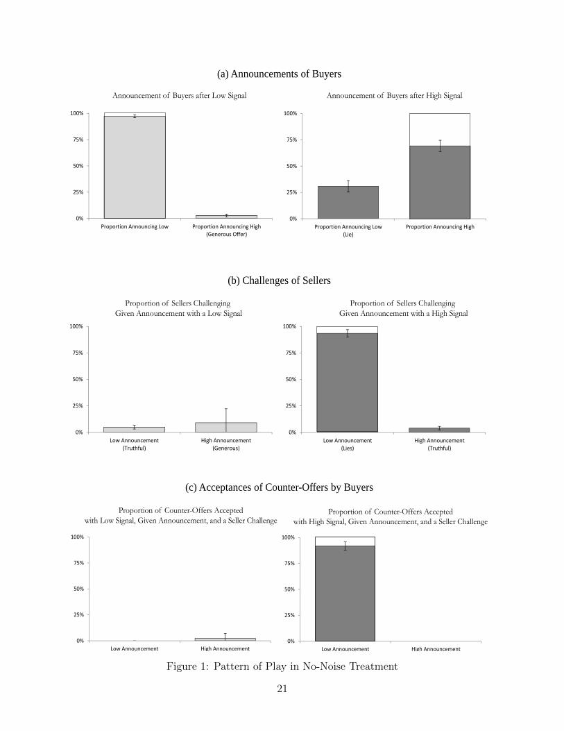
Figure 1 displays the patterns of play we observed in the no-noise treatment of the ex-
periment. The left column examines play when an individual receives a low signal while the
right side examines play when an individual receives a high signal. Panel (a) summarizes
B’s announcement decision, Panel (b) summarizes S’s challenge decision, and Panel (c) sum-
marizes B’s decision to accept or reject counter-offers. The error bars show 95% confidence
intervals of each proportion with standard errors clustered at the individual level.
19
Panel (a) shows that after a low signal, 97.2% of individuals announce that the value
is low. By contrast, after a high signal, 30.8% deviate from the theoretical prediction of
Hypothesis 1 and lie. We discuss this deviation from truth-telling in greater detail below
after detailing play in the other stages of the game.
Panel (b) shows the proportion of announcements that are challenged after each combi-
nation of announcement and signal. As can be seen, a low announcement with a low signal is
challenged only 4.1% of the time while a high announcement with a high signal is challenged
only 4.8% of the time. This implies that inappropriate challenges rarely occur in the data.
By contrast, S’s challenge a low announcement with a high signal 93.4% of the time implying
that S’s almost always make appropriate challenges.
Finally, Panel (c) shows the proportion of counter-offers that are accepted for each com-
bination of announcement and signal. In the case of a high signal, B’s always reject counter-
offers after truthful announcements and almost always accept counter-iffers after a lie. In
the case of a low signal, B’s always reject challenges after a low announcement.
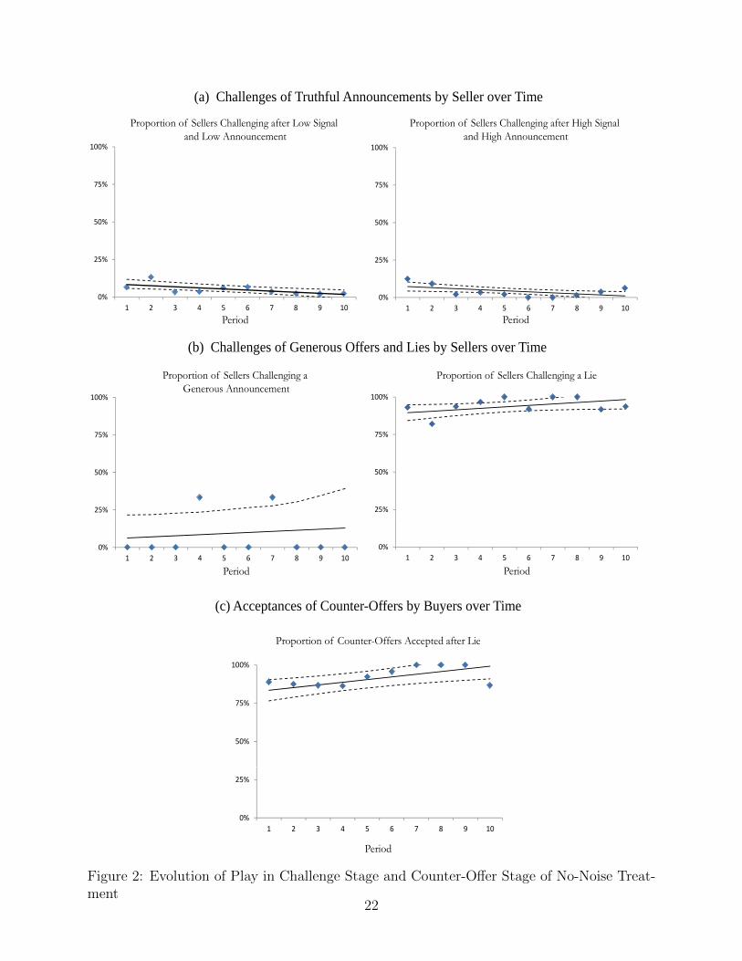
While there are small deviations from the theoretical predictions of the model in the
challenge stage and counter-offer stage, these deviations tend to vanish over time. Panel
(a) of Figure 2 tracks the proportion of truthful announcements that are challenged in each
period. This data is overlayed with the predictions and 95% confidence intervals from a
simple linear random effects regression that regresses the challenge decision on the period.
As can be seen, challenges of truthful announcements are diminishing and the proportion of
truthful announcements that are challenged is not significantly different from the theoretical
prediction of 0% by period 10. Similarly, as seen on the right side of Panel (b), challenges
of lies are increasing over time and the proportion of lies is not significantly different to the
theoretical prediction of 100% by period 10. Taken together, the data strongly supports the
appropriate-challenge condition.
Panel (c) of Figure 2 tracks the proportion of counter-offers that are accepted after a lie
over time using the same construction of the prediction line and 95% confidence intervals
as in the previous panels. While some B’s initially reject counter-offers, the proportion of
counter-offers being accepted increases over time and is not significantly different to the
theoretical prediction by period 10. Thus, there is strong evidence that the counter-offer
condition is met in the data.
Given that the appropriate-challenge condition and the counter-offer condition hold, B’s
have pecuniary incentives to announce truthfully by construction of the mechanism. Thus,
we might expect that lies converge to zero over time. Figure 3 shows that this is not the
case. As can be seen in Panel (a), the proportion of B’s who are lying is indeed slightly
decreasing over time. However, this proportion is above 20% and significantly different from
20
0%
25%
50%
75%
100%
Low Announcement(Lie)
High Announcement(Truthful)
0%
25%
50%
75%
100%
Low Announcement(Truthful)
High Announcement(Generous)
Proportion of Counter-Offers Acceptedwith Low Signal, Given Announcement, and a Seller Challenge
Proportion of Counter-Offers Acceptedwith High Signal, Given Announcement, and a Seller Challenge
0%
25%
50%
75%
100%
Low Announcement(Lies)
High Announcement(Truthful)
0%
25%
50%
75%
100%
Low Announcement(Truthful)
High Announcement(Generous)
Proportion of Sellers Challenging Given Announcement with a Low Signal
Proportion of Sellers Challenging Given Announcement with a High Signal
(c) Acceptances of Counter-Offers by Buyers
(b) Challenges of Sellers
0%
25%
50%
75%
100%
Proportion Announcing Low(Lie)
Proportion Announcing High
0%
25%
50%
75%
100%
Proportion Announcing Low Proportion Announcing High(Generous Offer)
Announcement of Buyers after Low Signal Announcement of Buyers after High Signal
(a) Announcements of Buyers
Figure 1: Pattern of Play in No-Noise Treatment
21
100% 100%
Proportion of Sellers Challenging after Low Signal and Low Announcement
Proportion of Sellers Challenging after High Signal and High Announcement
(a) Challenges of Truthful Announcements by Seller over Time
25%
50%
75%
100%
25%
50%
75%
100%
100%100%
Proportion of Sellers Challenging a Generous Announcement
Proportion of Sellers Challenging a Lie
0%
1 2 3 4 5 6 7 8 9 10
0%
1 2 3 4 5 6 7 8 9 10
Period Period
(b) Challenges of Generous Offers and Lies by Sellers over Time
25%
50%
75%
100%
25%
50%
75%
100%
Proportion of Counter-Offers Accepted after Lie
0%
1 2 3 4 5 6 7 8 9 10
0%
1 2 3 4 5 6 7 8 9 10
Period Period
(c) Acceptances of Counter-Offers by Buyers over Time
50%
75%
100%
Proportion of Counter Offers Accepted after Lie
0%
25%
1 2 3 4 5 6 7 8 9 10
Period
Figure 2: Evolution of Play in Challenge Stage and Counter-Offer Stage of No-Noise Treat-ment
22
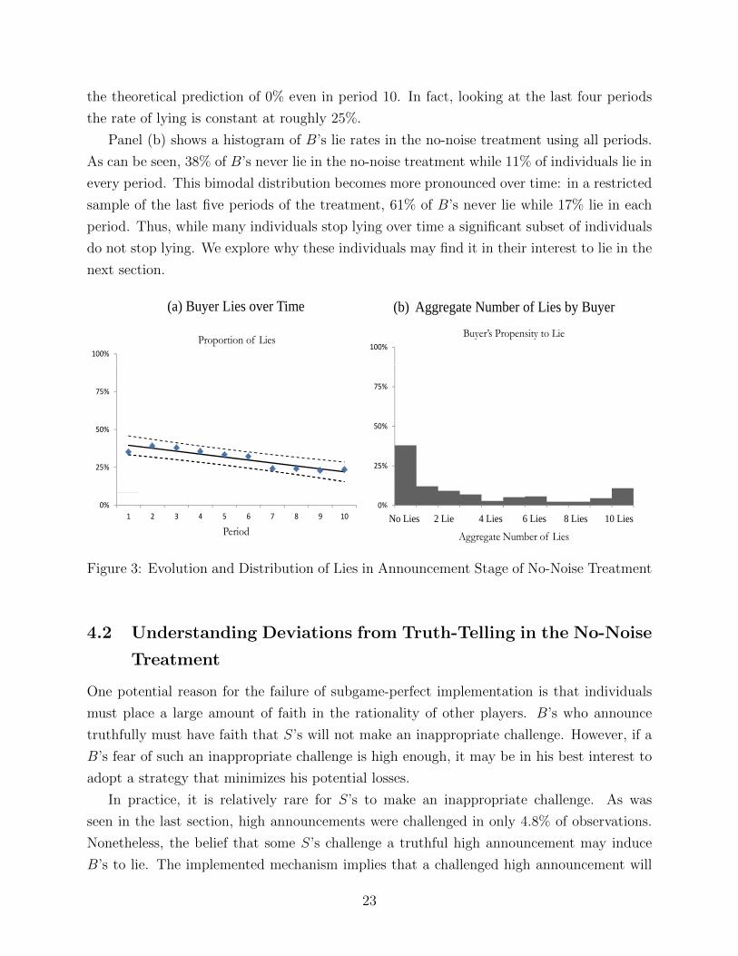
the theoretical prediction of 0% even in period 10. In fact, looking at the last four periods
the rate of lying is constant at roughly 25%.
Panel (b) shows a histogram of B’s lie rates in the no-noise treatment using all periods.
As can be seen, 38% of B’s never lie in the no-noise treatment while 11% of individuals lie in
every period. This bimodal distribution becomes more pronounced over time: in a restricted
sample of the last five periods of the treatment, 61% of B’s never lie while 17% lie in each
period. Thus, while many individuals stop lying over time a significant subset of individuals
do not stop lying. We explore why these individuals may find it in their interest to lie in the
next section.
100%100%
Buyer’s Propensity to Make Generous Announcements Buyer’s Propensity to Lie
(b) Aggregate Number of Lies by Buyer
100%
Proportion of Lies
(a) Buyer Lies over Time
25%
50%
75%
25%
50%
75%
25%
50%
75%
0%
0 2 4 6 8 10
0%
0 2 4 6 8 10No Lies 2 Lie 4 Lies 6 Lies 8 Lies 10 Lies No Lies 2 Lie 4 Lies 6 Lies 8 Lies 10 Lies
Aggregate Number of Generous Announcements Aggregate Number of Lies
0%
1 2 3 4 5 6 7 8 9 1010
Period
Figure 3: Evolution and Distribution of Lies in Announcement Stage of No-Noise Treatment
4.2 Understanding Deviations from Truth-Telling in the No-Noise
Treatment
One potential reason for the failure of subgame-perfect implementation is that individuals
must place a large amount of faith in the rationality of other players. B’s who announce
truthfully must have faith that S’s will not make an inappropriate challenge. However, if a
B’s fear of such an inappropriate challenge is high enough, it may be in his best interest to
adopt a strategy that minimizes his potential losses.
In practice, it is relatively rare for S’s to make an inappropriate challenge. As was
seen in the last section, high announcements were challenged in only 4.8% of observations.
Nonetheless, the belief that some S’s challenge a truthful high announcement may induce
B’s to lie. The implemented mechanism implies that a challenged high announcement will
23
lead to relatively large losses for B regardless of whether B accepts or rejects the challenge.
If B accepts the challenge, he will earn 70 - 75 - 25 = -30; if he rejects the challenge, he will
earn -25. These losses contrast sharply with the payoff of 20 that B can guarantee himself
by lying, being challenged by S, and accepting the counter-offer.
Looking at the beliefs data of B, it appears that the fear of inappropriate challenges is
indeed an important determinant of lies. Table 2 reports the results of regression analysis
where the dependent variable is 1 if B lies after the high signal and 0 if B makes a truthful
announcement. This variable is regressed on the belief that a lie will be challenged and the
belief that a truthful announcement will be challenged. To allow for potential non-linearities
in the beliefs data we treat B’s beliefs as categorical data and split the 4-point Likert scale
into a series of dummy variables. We use the category “Never” as the omitted dummy
category. Column (1) reports the results of a simple linear probability model with errors
clustered at the individual level. Column (2) reports the results of a fixed effects regression
with both time and individual level fixed effects.
As can be seen in column (1), B’s belief about the likelihood that he will be challenged
after a truthful announcement is a good predictor of his likelihood of making a lie. B’s are
39.7 (59) percentage points more likely to lie if they believe that a truthful announcement
is “Likely” (“Always”) to be challenged relative to an individual who believes a truthful
announcement will “Never” be challenged. The probability of making a lie is increasing as
an individual’s beliefs becomes more pessimistic suggesting a monotonic relationship between
beliefs and lies. This conclusion also holds if we control for individual and time fixes effects
(see column 2)
4.2.1 Precise quantification of beliefs to better understand buyer lies
To explore further the way in which beliefs may be guiding lies in the no-noise treatment we
ran an additional experiment in which we elicited probabilistic beliefs of being challenged
using an incentive-compatible elicitation mechanism developed in Karni (2009).18 In this
follow-up treatment, we restricted attention to only the no-noise treatment and ran additional
periods to study convergence. We ran two sessions with 30 periods and two sessions with 40
18Akin to a standard BDM mechanism (Becker, DeGroot & Marschak, 1964), the belief elicitation mechanismgives B a dominant strategy to announce his true beliefs by using B’s reported belief to assign him toone of two lotteries — one that is contingent on S’s challenge decision and one that is independent of thisdecision — across a set of binary lottery pairs. We randomly select one of these lottery pairs to be playedso that beliefs impact the assignment of B to a lottery but not the explicit characteristics of this lottery.We use the strategy method in this follow up experiment for S’s challenge decisions as we want to elicitincentive-compatible beliefs from B about the likelihood of being challenged after a truthful announcementand after a lie. To do so we need to know S’s challenge decision for both announcements. See the appendixfor full details.
24
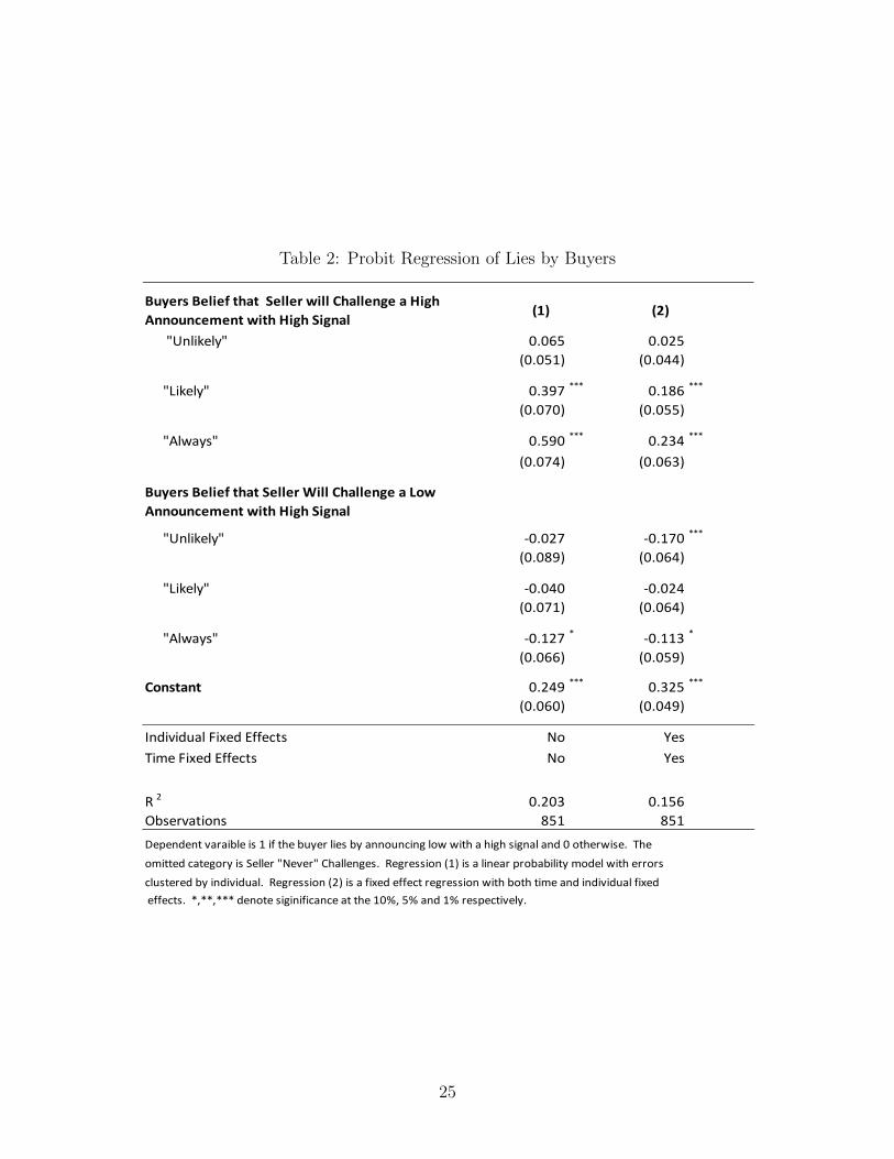
Table 2: Probit Regression of Lies by Buyers
Buyers Belief that Seller will Challenge a High
Announcement with High Signal(1) (2)
"Unlikely" 0.065 0.025
(0.051) (0.044)
"Likely" 0.397 *** 0.186 ***
(0.070) (0.055)
"Always" 0.590 *** 0.234 ***
(0.074) (0.063)
Buyers Belief that Seller Will Challenge a Low
Announcement with High Signal
"Unlikely" ‐0.027 ‐0.170 ***
(0.089) (0.064)
"Likely" ‐0.040 ‐0.024
(0.071) (0.064)
"Always" ‐0.127 * ‐0.113 *
(0.066) (0.059)
Constant 0.249 *** 0.325 ***
(0.060) (0.049)
Individual Fixed Effects No Yes
Time Fixed Effects No Yes
R 2 0.203 0.156
Observations 851 851
Dependent varaible is 1 if the buyer lies by announcing low with a high signal and 0 otherwise. The
omitted category is Seller "Never" Challenges. Regression (1) is a linear probability model with errors
clustered by individual. Regression (2) is a fixed effect regression with both time and individual fixed
effects. *,**,*** denote siginificance at the 10%, 5% and 1% respectively.
25
periods with random matching across periods. A total of 90 individuals participated in the
experiment. The details of this elicitation mechanism can be found in the appendix.19
Result 2 The majority of B’s have pessimistic beliefs about being challenged after a truthful
announcement of 70. The majority of B’s have optimistic beliefs about being challenged after
a lie of 20.
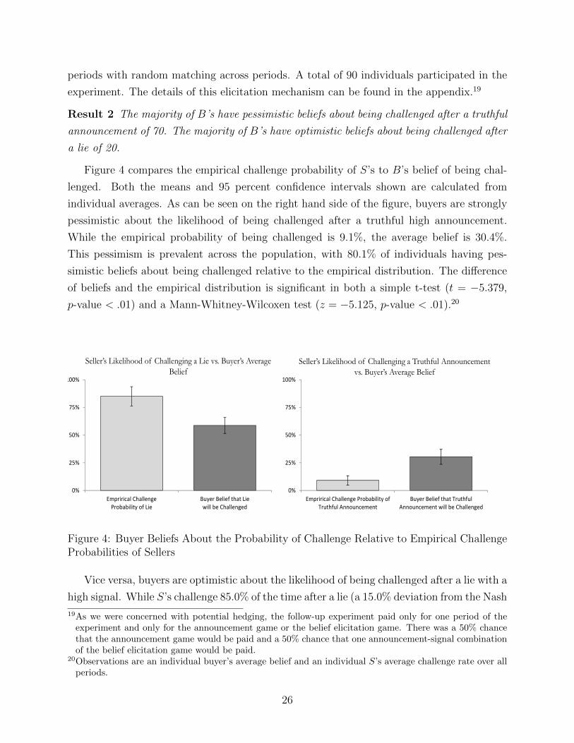
Figure 4 compares the empirical challenge probability of S’s to B’s belief of being chal-
lenged. Both the means and 95 percent confidence intervals shown are calculated from
individual averages. As can be seen on the right hand side of the figure, buyers are strongly
pessimistic about the likelihood of being challenged after a truthful high announcement.
While the empirical probability of being challenged is 9.1%, the average belief is 30.4%.
This pessimism is prevalent across the population, with 80.1% of individuals having pes-
simistic beliefs about being challenged relative to the empirical distribution. The difference
of beliefs and the empirical distribution is significant in both a simple t-test (t = −5.379,
p-value < .01) and a Mann-Whitney-Wilcoxen test (z = −5.125, p-value < .01).20
0%
25%
50%
75%
100%
Emprirical ChallengeProbability of Lie
Buyer Belief that Liewill be Challenged
0%
25%
50%
75%
100%
Emprirical Challenge Probability ofTruthful Announcement
Buyer Belief that TruthfulAnnouncement will be Challenged
Seller’s Likelihood of Challenging a Lie vs. Buyer’s AverageBelief
Seller’s Likelihood of Challenging a Truthful Announcementvs. Buyer’s Average Belief
Figure 4: Buyer Beliefs About the Probability of Challenge Relative to Empirical ChallengeProbabilities of Sellers
Vice versa, buyers are optimistic about the likelihood of being challenged after a lie with a
high signal. While S’s challenge 85.0% of the time after a lie (a 15.0% deviation from the Nash
19As we were concerned with potential hedging, the follow-up experiment paid only for one period of theexperiment and only for the announcement game or the belief elicitation game. There was a 50% chancethat the announcement game would be paid and a 50% chance that one announcement-signal combinationof the belief elicitation game would be paid.
20Observations are an individual buyer’s average belief and an individual S’s average challenge rate over allperiods.
26
Equilibrium), the average belief is 58.7% (a 41.3% deviation from the Nash Equilibrium).
This optimism is again prevalent across the population, with 76.7% of individuals having
optimistic beliefs about being challenged relative to the empirical distribution. The difference
between beliefs and the empirical distribution is again significant (t-test: t = 4.703, p-value
< .01; Mann-Whitney-Wilcoxen test: z = 5.56, p-value < .01).
Given the optimistic beliefs about outcomes after a lie and pessimistic beliefs about
outcomes after truthful announcing, a natural hypothesis is that B’s may believe that they
are monetarily better off lying than telling the truth. To test this hypothesis, we use B’s
reported beliefs to compute the expected value of lying and telling the truth after a high
signal if B’s respond optimally to a subsequent challenge. We next take the difference
between these expected values to estimate the expected monetary gain from truth-telling.
Result 3 The majority of B’s believe they have a higher expected value from lying compared
to truth-telling after a high signal. B’s with more optimistic beliefs about being challenged
after a lie and more pessimistic beliefs about being challenged after a truthful announcement
are more likely to lie.
Figure 5 show the empirical cumulative density functions of the expected gain from truth-
telling split between observations where an individuals is lying (N = 543) and observations
where an individual is telling the truth (N = 491).21 As can be seen, the empirical CDF of
the expected monetary gain from truth-telling for individuals who tell the truth first order
stochastically dominates the CDF for individuals who lie, suggesting that heterogeneity in
beliefs is an important factor in the decision to announce truthfully.22 For both distributions,
however, the proportion of individuals where the expected monetary gain from truth-telling
is negative is large, with 79.2% (72.7%) of observations where the buyer lies (tells the truth)
falling into this category.
One potential reason for the high level of pessimism seen in B’s beliefs about being
inappropriately challenged is that at least a subset of individuals are choosing announcement
strategies that limit their ability to learn over time. 28.9% of individuals lie in each of the
last 10 periods of the session and in at least 90% of periods overall. These individuals account
for 60.7% of overall lies and 71.7% of lies that occur in the last 10 periods. As a B who
21We restrict attention to observations where (i) the buyer believed that announcing low with a high sig-nal had a higher chance of being challenged than announcing high with a low signal and (ii) the buyerannounced low with a low signal. There is a very small fraction of individuals in our sample that do notsatisfy these plausibility conditions. If we include them, all the qualitative results remain the same andsignificant.
22These distributions are significantly different in a bootstrapped version of the Mann-Whitney-Wilcoxentest where we randomly sampled a single period from each buyer in each iteration. p-value < .01. SeeDatta & Satten (2005) for a discussion.
27
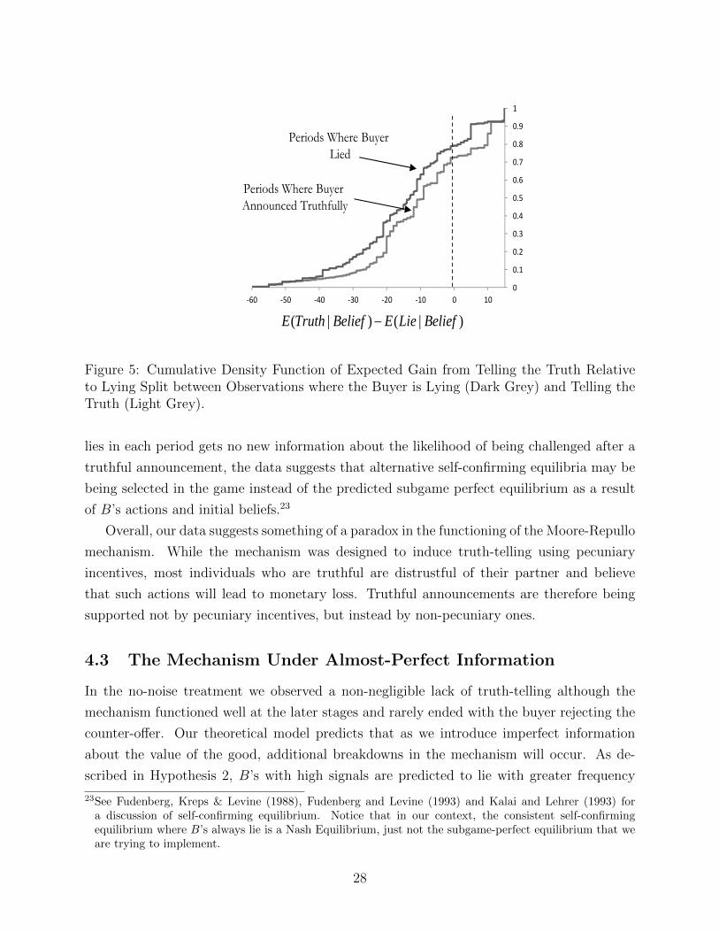
0
0.1
0.2
0.3
0.4
0.5
0.6
0.7
0.8
0.9
1
‐60 ‐50 ‐40 ‐30 ‐20 ‐10 0 10
( | ) ( | )E Truth Belief E Lie Belief
Cumulative Density Function of Expected Value of Telling the Truth
Periods Where BuyerLied
Periods Where BuyerAnnounced Truthfully
Figure 5: Cumulative Density Function of Expected Gain from Telling the Truth Relativeto Lying Split between Observations where the Buyer is Lying (Dark Grey) and Telling theTruth (Light Grey).
lies in each period gets no new information about the likelihood of being challenged after a
truthful announcement, the data suggests that alternative self-confirming equilibria may be
being selected in the game instead of the predicted subgame perfect equilibrium as a result
of B’s actions and initial beliefs.23
Overall, our data suggests something of a paradox in the functioning of the Moore-Repullo
mechanism. While the mechanism was designed to induce truth-telling using pecuniary
incentives, most individuals who are truthful are distrustful of their partner and believe
that such actions will lead to monetary loss. Truthful announcements are therefore being
supported not by pecuniary incentives, but instead by non-pecuniary ones.
4.3 The Mechanism Under Almost-Perfect Information
In the no-noise treatment we observed a non-negligible lack of truth-telling although the
mechanism functioned well at the later stages and rarely ended with the buyer rejecting the
counter-offer. Our theoretical model predicts that as we introduce imperfect information
about the value of the good, additional breakdowns in the mechanism will occur. As de-
scribed in Hypothesis 2, B’s with high signals are predicted to lie with greater frequency
23See Fudenberg, Kreps & Levine (1988), Fudenberg and Levine (1993) and Kalai and Lehrer (1993) fora discussion of self-confirming equilibrium. Notice that in our context, the consistent self-confirmingequilibrium where B’s always lie is a Nash Equilibrium, just not the subgame-perfect equilibrium that weare trying to implement.
28
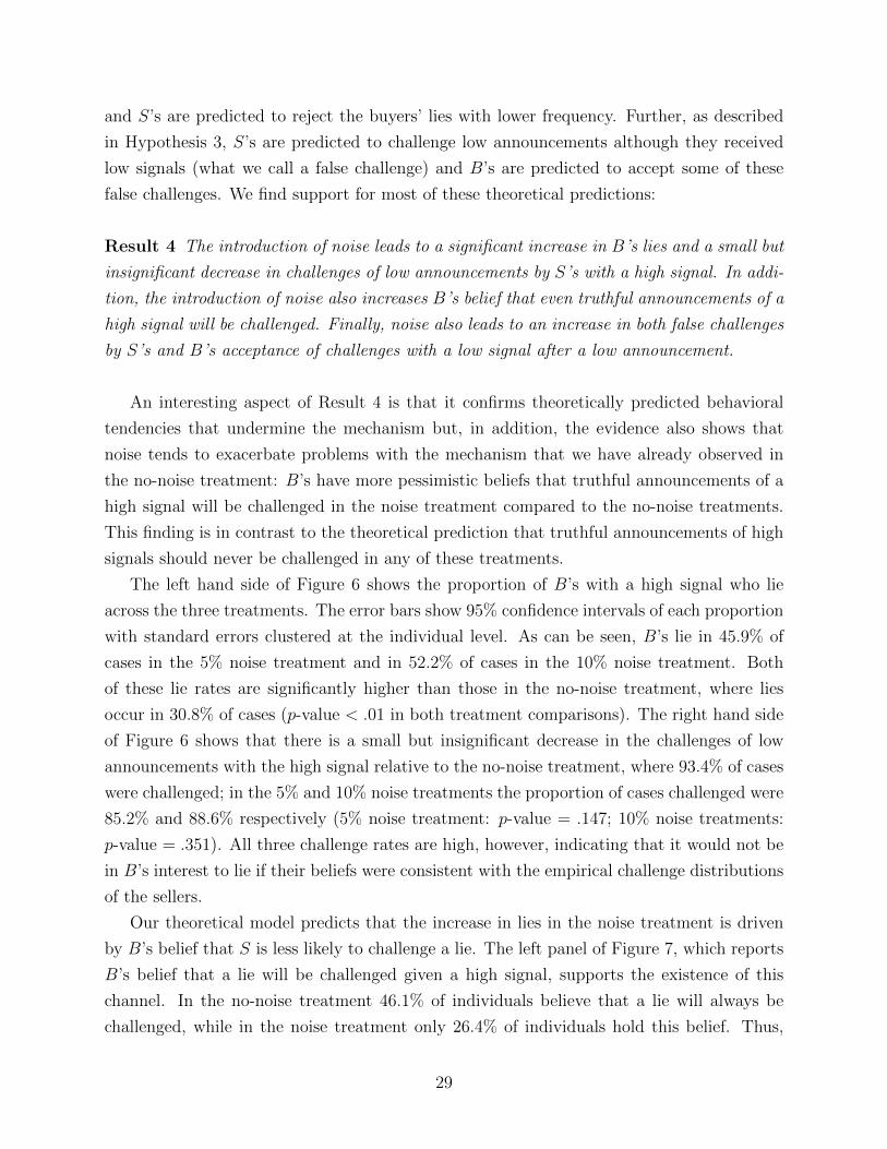
and S’s are predicted to reject the buyers’ lies with lower frequency. Further, as described
in Hypothesis 3, S’s are predicted to challenge low announcements although they received
low signals (what we call a false challenge) and B’s are predicted to accept some of these
false challenges. We find support for most of these theoretical predictions:
Result 4 The introduction of noise leads to a significant increase in B’s lies and a small but
insignificant decrease in challenges of low announcements by S’s with a high signal. In addi-
tion, the introduction of noise also increases B’s belief that even truthful announcements of a
high signal will be challenged. Finally, noise also leads to an increase in both false challenges
by S’s and B’s acceptance of challenges with a low signal after a low announcement.
An interesting aspect of Result 4 is that it confirms theoretically predicted behavioral
tendencies that undermine the mechanism but, in addition, the evidence also shows that
noise tends to exacerbate problems with the mechanism that we have already observed in
the no-noise treatment: B’s have more pessimistic beliefs that truthful announcements of a
high signal will be challenged in the noise treatment compared to the no-noise treatments.
This finding is in contrast to the theoretical prediction that truthful announcements of high
signals should never be challenged in any of these treatments.
The left hand side of Figure 6 shows the proportion of B’s with a high signal who lie
across the three treatments. The error bars show 95% confidence intervals of each proportion
with standard errors clustered at the individual level. As can be seen, B’s lie in 45.9% of
cases in the 5% noise treatment and in 52.2% of cases in the 10% noise treatment. Both
of these lie rates are significantly higher than those in the no-noise treatment, where lies
occur in 30.8% of cases (p-value < .01 in both treatment comparisons). The right hand side
of Figure 6 shows that there is a small but insignificant decrease in the challenges of low
announcements with the high signal relative to the no-noise treatment, where 93.4% of cases
were challenged; in the 5% and 10% noise treatments the proportion of cases challenged were
85.2% and 88.6% respectively (5% noise treatment: p-value = .147; 10% noise treatments:
p-value = .351). All three challenge rates are high, however, indicating that it would not be
in B’s interest to lie if their beliefs were consistent with the empirical challenge distributions
of the sellers.
Our theoretical model predicts that the increase in lies in the noise treatment is driven
by B’s belief that S is less likely to challenge a lie. The left panel of Figure 7, which reports
B’s belief that a lie will be challenged given a high signal, supports the existence of this
channel. In the no-noise treatment 46.1% of individuals believe that a lie will always be
challenged, while in the noise treatment only 26.4% of individuals hold this belief. Thus,
29
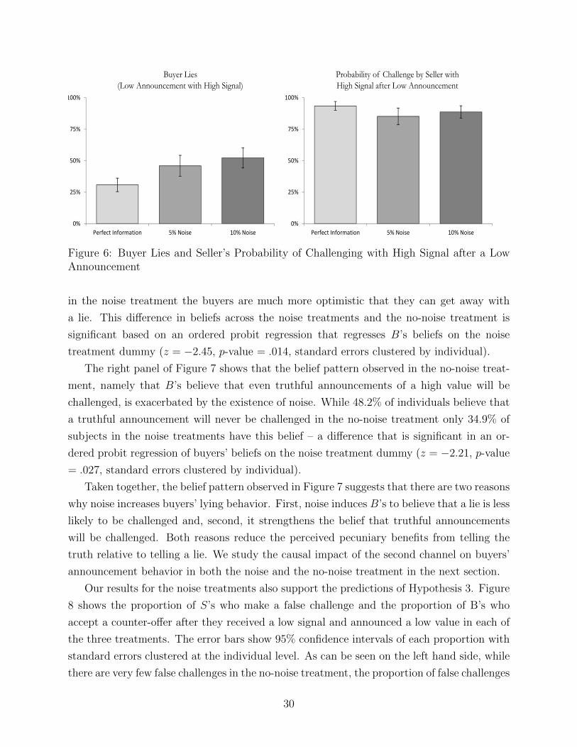
0%
25%
50%
75%
100%
Perfect Information 5% Noise 10% Noise
0%
25%
50%
75%
100%
Perfect Information 5% Noise 10% Noise
Buyer Lies(Low Announcement with High Signal)
Probability of Challenge by Seller withHigh Signal after Low Announcement
Figure 6: Buyer Lies and Seller’s Probability of Challenging with High Signal after a LowAnnouncement
in the noise treatment the buyers are much more optimistic that they can get away with
a lie. This difference in beliefs across the noise treatments and the no-noise treatment is
significant based on an ordered probit regression that regresses B’s beliefs on the noise
treatment dummy (z = −2.45, p-value = .014, standard errors clustered by individual).
The right panel of Figure 7 shows that the belief pattern observed in the no-noise treat-
ment, namely that B’s believe that even truthful announcements of a high value will be
challenged, is exacerbated by the existence of noise. While 48.2% of individuals believe that
a truthful announcement will never be challenged in the no-noise treatment only 34.9% of
subjects in the noise treatments have this belief – a difference that is significant in an or-
dered probit regression of buyers’ beliefs on the noise treatment dummy (z = −2.21, p-value
= .027, standard errors clustered by individual).
Taken together, the belief pattern observed in Figure 7 suggests that there are two reasons
why noise increases buyers’ lying behavior. First, noise induces B’s to believe that a lie is less
likely to be challenged and, second, it strengthens the belief that truthful announcements
will be challenged. Both reasons reduce the perceived pecuniary benefits from telling the
truth relative to telling a lie. We study the causal impact of the second channel on buyers’
announcement behavior in both the noise and the no-noise treatment in the next section.
Our results for the noise treatments also support the predictions of Hypothesis 3. Figure
8 shows the proportion of S’s who make a false challenge and the proportion of B’s who
accept a counter-offer after they received a low signal and announced a low value in each of
the three treatments. The error bars show 95% confidence intervals of each proportion with
standard errors clustered at the individual level. As can be seen on the left hand side, while
there are very few false challenges in the no-noise treatment, the proportion of false challenges
30
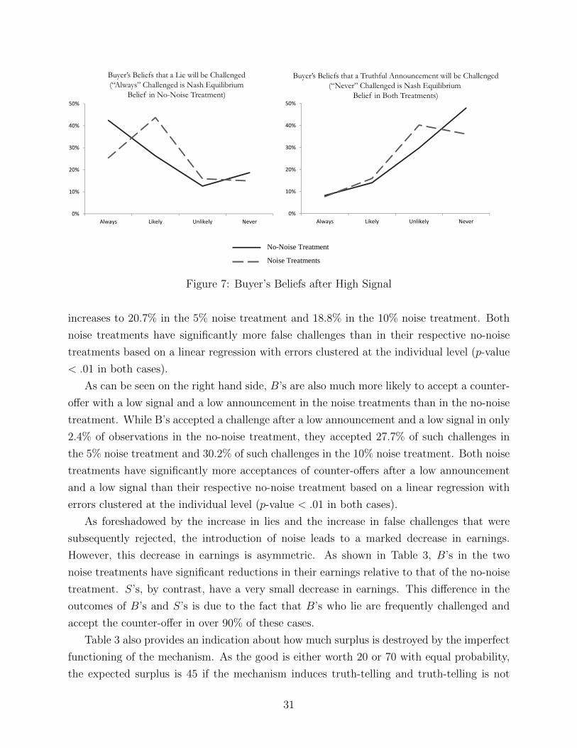
0%
10%
20%
30%
40%
50%
Always Likely Unlikely Never
0%
10%
20%
30%
40%
50%
Always Likely Unlikely Never
Buyer’s Beliefs that a Lie will be Challenged(“Always” Challenged is Nash Equilibrium
Belief in No-Noise Treatment)
Buyer’s Beliefs that a Truthful Announcement will be Challenged(“Never” Challenged is Nash Equilibrium
Belief in Both Treatments)
No-Noise Treatment
Noise Treatments
Figure 7: Buyer’s Beliefs after High Signal
increases to 20.7% in the 5% noise treatment and 18.8% in the 10% noise treatment. Both
noise treatments have significantly more false challenges than in their respective no-noise
treatments based on a linear regression with errors clustered at the individual level (p-value
< .01 in both cases).
As can be seen on the right hand side, B’s are also much more likely to accept a counter-
offer with a low signal and a low announcement in the noise treatments than in the no-noise
treatment. While B’s accepted a challenge after a low announcement and a low signal in only
2.4% of observations in the no-noise treatment, they accepted 27.7% of such challenges in
the 5% noise treatment and 30.2% of such challenges in the 10% noise treatment. Both noise
treatments have significantly more acceptances of counter-offers after a low announcement
and a low signal than their respective no-noise treatment based on a linear regression with
errors clustered at the individual level (p-value < .01 in both cases).
As foreshadowed by the increase in lies and the increase in false challenges that were
subsequently rejected, the introduction of noise leads to a marked decrease in earnings.
However, this decrease in earnings is asymmetric. As shown in Table 3, B’s in the two
noise treatments have significant reductions in their earnings relative to that of the no-noise
treatment. S’s, by contrast, have a very small decrease in earnings. This difference in the
outcomes of B’s and S’s is due to the fact that B’s who lie are frequently challenged and
accept the counter-offer in over 90% of these cases.
Table 3 also provides an indication about how much surplus is destroyed by the imperfect
functioning of the mechanism. As the good is either worth 20 or 70 with equal probability,
the expected surplus is 45 if the mechanism induces truth-telling and truth-telling is not
31
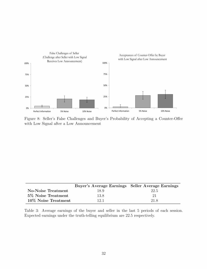
0%
25%
50%
75%
100%
Perfect Information 5% Noise 10% Noise
0%
25%
50%
75%
100%
Perfect Information 5% Noise 10% Noise
False Challenges of Seller (Challenge after Seller with Low Signal
Receives Low Announcement)
Acceptances of Counter-Offer by Buyer with Low Signal after Low Announcement
Figure 8: Seller’s False Challenges and Buyer’s Probability of Accepting a Counter-Offerwith Low Signal after a Low Announcement
Buyer’s Average Earnings Seller Average EarningsNo-Noise Treatment 18.9 22.55% Noise Treatment 13.8 2110% Noise Treatment 12.1 21.8
Table 3: Average earnings of the buyer and seller in the last 5 periods of each session.Expected earnings under the truth-telling equilibrium are 22.5 respectively.
32
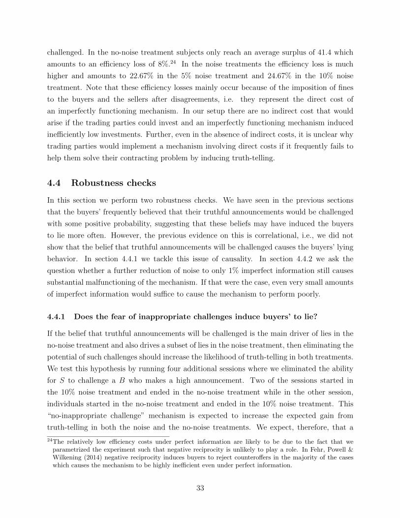
challenged. In the no-noise treatment subjects only reach an average surplus of 41.4 which
amounts to an efficiency loss of 8%.24 In the noise treatments the efficiency loss is much
higher and amounts to 22.67% in the 5% noise treatment and 24.67% in the 10% noise
treatment. Note that these efficiency losses mainly occur because of the imposition of fines
to the buyers and the sellers after disagreements, i.e. they represent the direct cost of
an imperfectly functioning mechanism. In our setup there are no indirect cost that would
arise if the trading parties could invest and an imperfectly functioning mechanism induced
inefficiently low investments. Further, even in the absence of indirect costs, it is unclear why
trading parties would implement a mechanism involving direct costs if it frequently fails to
help them solve their contracting problem by inducing truth-telling.
4.4 Robustness checks
In this section we perform two robustness checks. We have seen in the previous sections
that the buyers’ frequently believed that their truthful announcements would be challenged
with some positive probability, suggesting that these beliefs may have induced the buyers
to lie more often. However, the previous evidence on this is correlational, i.e., we did not
show that the belief that truthful announcements will be challenged causes the buyers’ lying
behavior. In section 4.4.1 we tackle this issue of causality. In section 4.4.2 we ask the
question whether a further reduction of noise to only 1% imperfect information still causes
substantial malfunctioning of the mechanism. If that were the case, even very small amounts
of imperfect information would suffice to cause the mechanism to perform poorly.
4.4.1 Does the fear of inappropriate challenges induce buyers’ to lie?
If the belief that truthful announcements will be challenged is the main driver of lies in the
no-noise treatment and also drives a subset of lies in the noise treatment, then eliminating the
potential of such challenges should increase the likelihood of truth-telling in both treatments.
We test this hypothesis by running four additional sessions where we eliminated the ability
for S to challenge a B who makes a high announcement. Two of the sessions started in
the 10% noise treatment and ended in the no-noise treatment while in the other session,
individuals started in the no-noise treatment and ended in the 10% noise treatment. This
“no-inappropriate challenge” mechanism is expected to increase the expected gain from
truth-telling in both the noise and the no-noise treatments. We expect, therefore, that a
24The relatively low efficiency costs under perfect information are likely to be due to the fact that weparametrized the experiment such that negative reciprocity is unlikely to play a role. In Fehr, Powell &Wilkening (2014) negative reciprocity induces buyers to reject counteroffers in the majority of the caseswhich causes the mechanism to be highly inefficient even under perfect information.
33
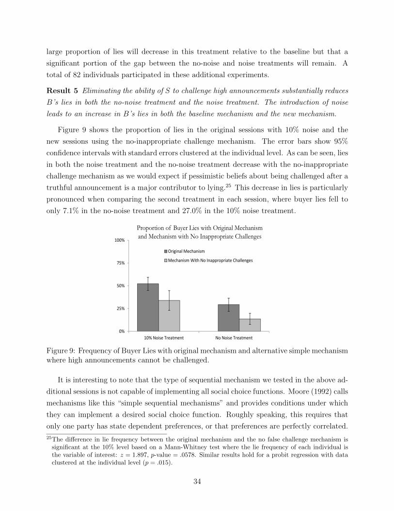
large proportion of lies will decrease in this treatment relative to the baseline but that a
significant portion of the gap between the no-noise and noise treatments will remain. A
total of 82 individuals participated in these additional experiments.
Result 5 Eliminating the ability of S to challenge high announcements substantially reduces
B’s lies in both the no-noise treatment and the noise treatment. The introduction of noise
leads to an increase in B’s lies in both the baseline mechanism and the new mechanism.
Figure 9 shows the proportion of lies in the original sessions with 10% noise and the
new sessions using the no-inappropriate challenge mechanism. The error bars show 95%
confidence intervals with standard errors clustered at the individual level. As can be seen, lies
in both the noise treatment and the no-noise treatment decrease with the no-inappropriate
challenge mechanism as we would expect if pessimistic beliefs about being challenged after a
truthful announcement is a major contributor to lying.25 This decrease in lies is particularly
pronounced when comparing the second treatment in each session, where buyer lies fell to
only 7.1% in the no-noise treatment and 27.0% in the 10% noise treatment.
0%
25%
50%
75%
100%
10% Noise Treatment No Noise Treatment
Original Mechanism
Mechanism With No Inappropriate Challenges
Proportion of Buyer Lies with Original Mechanismand Mechanism with No Inappropriate Challenges
Figure 9: Frequency of Buyer Lies with original mechanism and alternative simple mechanismwhere high announcements cannot be challenged.
It is interesting to note that the type of sequential mechanism we tested in the above ad-
ditional sessions is not capable of implementing all social choice functions. Moore (1992) calls
mechanisms like this “simple sequential mechanisms” and provides conditions under which
they can implement a desired social choice function. Roughly speaking, this requires that
only one party has state dependent preferences, or that preferences are perfectly correlated.
25The difference in lie frequency between the original mechanism and the no false challenge mechanism issignificant at the 10% level based on a Mann-Whitney test where the lie frequency of each individual isthe variable of interest: z = 1.897, p-value = .0578. Similar results hold for a probit regression with dataclustered at the individual level (p = .015).
34
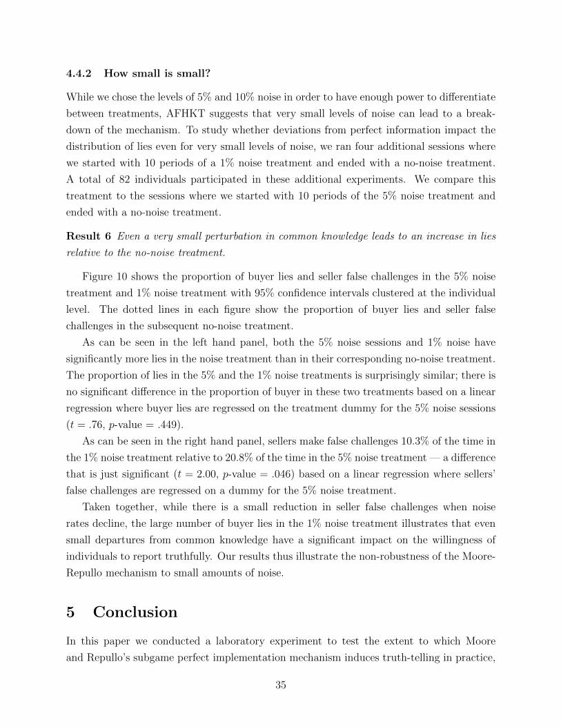
4.4.2 How small is small?
While we chose the levels of 5% and 10% noise in order to have enough power to differentiate
between treatments, AFHKT suggests that very small levels of noise can lead to a break-
down of the mechanism. To study whether deviations from perfect information impact the
distribution of lies even for very small levels of noise, we ran four additional sessions where
we started with 10 periods of a 1% noise treatment and ended with a no-noise treatment.
A total of 82 individuals participated in these additional experiments. We compare this
treatment to the sessions where we started with 10 periods of the 5% noise treatment and
ended with a no-noise treatment.
Result 6 Even a very small perturbation in common knowledge leads to an increase in lies
relative to the no-noise treatment.
Figure 10 shows the proportion of buyer lies and seller false challenges in the 5% noise
treatment and 1% noise treatment with 95% confidence intervals clustered at the individual
level. The dotted lines in each figure show the proportion of buyer lies and seller false
challenges in the subsequent no-noise treatment.
As can be seen in the left hand panel, both the 5% noise sessions and 1% noise have
significantly more lies in the noise treatment than in their corresponding no-noise treatment.
The proportion of lies in the 5% and the 1% noise treatments is surprisingly similar; there is
no significant difference in the proportion of buyer in these two treatments based on a linear
regression where buyer lies are regressed on the treatment dummy for the 5% noise sessions
(t = .76, p-value = .449).
As can be seen in the right hand panel, sellers make false challenges 10.3% of the time in
the 1% noise treatment relative to 20.8% of the time in the 5% noise treatment — a difference
that is just significant (t = 2.00, p-value = .046) based on a linear regression where sellers’
false challenges are regressed on a dummy for the 5% noise treatment.
Taken together, while there is a small reduction in seller false challenges when noise
rates decline, the large number of buyer lies in the 1% noise treatment illustrates that even
small departures from common knowledge have a significant impact on the willingness of
individuals to report truthfully. Our results thus illustrate the non-robustness of the Moore-
Repullo mechanism to small amounts of noise.
5 Conclusion
In this paper we conducted a laboratory experiment to test the extent to which Moore
and Repullo’s subgame perfect implementation mechanism induces truth-telling in practice,
35
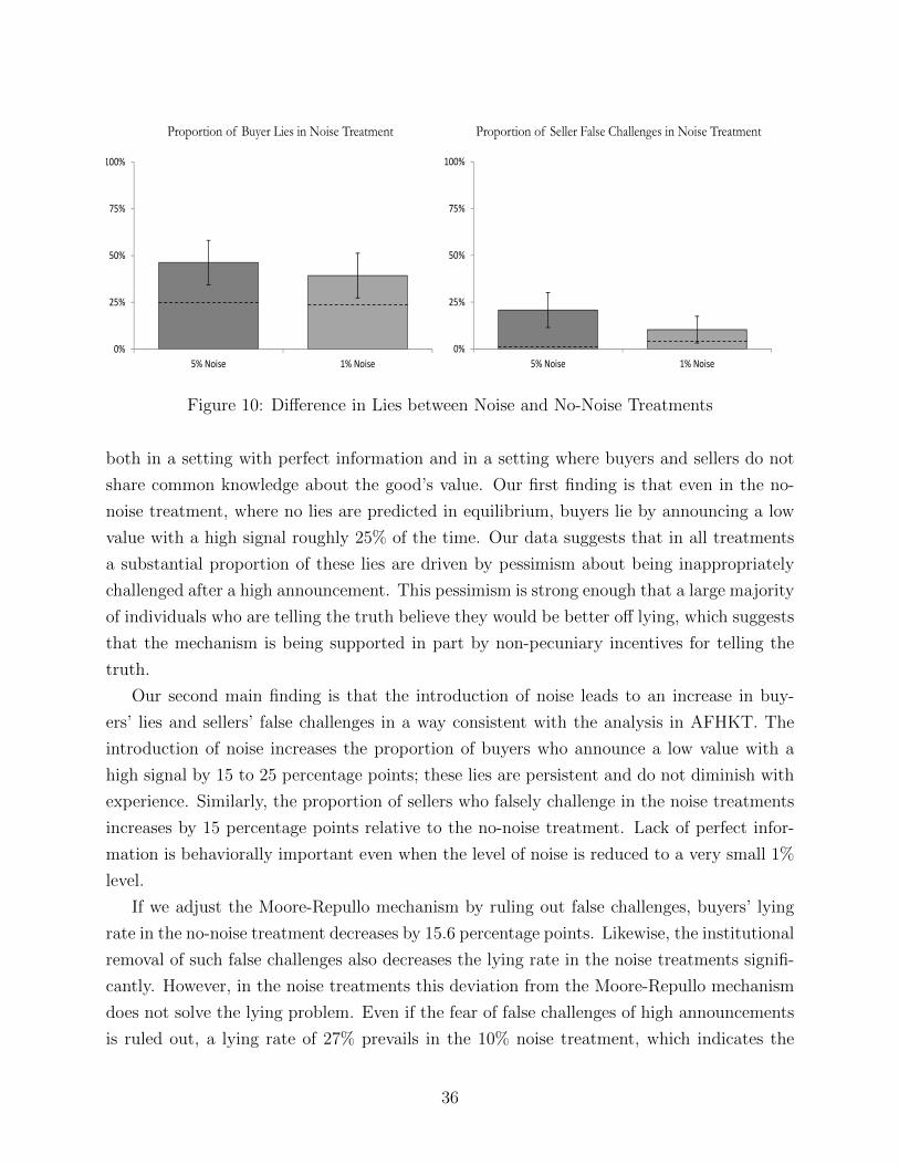
0%
25%
50%
75%
100%
5% Noise 1% Noise
0%
25%
50%
75%
100%
5% Noise 1% Noise
Proportion of Buyer Lies in Noise Treatment Proportion of Seller False Challenges in Noise Treatment
Figure 10: Difference in Lies between Noise and No-Noise Treatments
both in a setting with perfect information and in a setting where buyers and sellers do not
share common knowledge about the good’s value. Our first finding is that even in the no-
noise treatment, where no lies are predicted in equilibrium, buyers lie by announcing a low
value with a high signal roughly 25% of the time. Our data suggests that in all treatments
a substantial proportion of these lies are driven by pessimism about being inappropriately
challenged after a high announcement. This pessimism is strong enough that a large majority
of individuals who are telling the truth believe they would be better off lying, which suggests
that the mechanism is being supported in part by non-pecuniary incentives for telling the
truth.
Our second main finding is that the introduction of noise leads to an increase in buy-
ers’ lies and sellers’ false challenges in a way consistent with the analysis in AFHKT. The
introduction of noise increases the proportion of buyers who announce a low value with a
high signal by 15 to 25 percentage points; these lies are persistent and do not diminish with
experience. Similarly, the proportion of sellers who falsely challenge in the noise treatments
increases by 15 percentage points relative to the no-noise treatment. Lack of perfect infor-
mation is behaviorally important even when the level of noise is reduced to a very small 1%
level.
If we adjust the Moore-Repullo mechanism by ruling out false challenges, buyers’ lying
rate in the no-noise treatment decreases by 15.6 percentage points. Likewise, the institutional
removal of such false challenges also decreases the lying rate in the noise treatments signifi-
cantly. However, in the noise treatments this deviation from the Moore-Repullo mechanism
does not solve the lying problem. Even if the fear of false challenges of high announcements
is ruled out, a lying rate of 27% prevails in the 10% noise treatment, which indicates the
36
pervasive influence of uncertainty regarding the good’s value on lying behavior.
One important potential objection to our findings is that when parties themselves design a
mechanism one should be less concerned about the fears of irrationality that play a prominent
role in our experiment. As Eric Maskin suggested to us, when the parties are designing a
contract they may engage in all sorts of discussion about how the game might be played.
This is an important point to which we have two responses. First, pre-play communication
can naturally be modelled as a cheap-talk stage prior to the mechanisms studied in this
paper. To understand the benefits or otherwise of such communication one should, and
can, model this additional stage. Second, pre-play communication does not obviate the fact
that in our setting, players observe conditionally independent signals, and thus higher-order
beliefs are relevant to play in the game induced by the mechanism. The fact that the players
in the game designed the game itself does not alter the fact that common knowledge of the
underlying state — something that is not a design variable — is crucial to the success of
the mechanism. That said, understanding how pre-play communication intersects with the
issues studied in this paper is an enticing avenue for both theoretical and experimental work.
Our findings suggest several important avenues for future research, in addition to that
mentioned in the preceeding paragraph. First, the fact that individuals are willing to sacrifice
their material well-being to tell the truth suggests that preferences for honesty should help
implementation.26 Second, in view of the empirical relevance of common knowledge, it also
is important to design mechanisms that are robust to at least small amounts of imperfect
information about the good’s value. Third, it would be interesting to know (theoretically and
empirically) how the introduction of asset ownership affects the functioning of extensive form
mechanisms. In particular, asset ownership could be naturally modeled as an outside option
for the asset holder, which in turn would affect either party’s incentive to report the good’s
value truthfully or to challenge the other party. It would be interesting to see whether asset
ownership helps achieve better equilibrium outcomes that are also robust to introducing
small amounts of private information. Finally, similar experiments could be used to test
the robustness of other implementation mechanisms, starting with virtual implementation.
Overall, our analysis and findings in this paper raise a number of exciting issues to be tackled
by future research.
26Current research by Kartik, Tercieux and Holden (2014) suggests that when individuals have a knownpreference for honesty, full implementation can be achieved with simple mechanisms requiring only tworounds of iterated deletion of strictly dominated strategies.
37
References
Aghion, P., Fudenberg, D., Holden, R., Kunimoto, T. & Tercieux, O. (2012), ‘Subgame-
perfect implementation under value perturbations’, Quarterly Journal of Economics
127(4), 1843–1881.
Aghion, P. & Holden, R. (2011), ‘Incomplete contracts and the theory of the firm: What have
we learned over the past 25 years?’, Journal of Economic Perspectives 25(2), 181–197.
Andreoni, J. & Varian, H. (1999), ‘Pre–play contracting in the prisoners’ dilemma’, Proceed-
ings of the National Acadamy of Science of the United States of America 96, 10933–
10938.
Arifovic, J. & Ledyard, J. (2004), ‘Scaling up learning models in public good games’, Journal
of Public Economic Theory 6(2), 203–238.
Attiyeh, G., Franciosi, R. & Isaac, R. (2000), ‘Experiments with the pivot process for pro-
viding public goods’, Public Choice 102(1-2), 95–114.
Becker, G., DeGroot, M. H. & Marschak, J. (1964), ‘Measuring utility by a single-response
sequential method’, Behavioral Science 9(3), 226–232.
Blanco, M., Engelmann, D., Koch, A. K. & Normann, H.-T. (2010), ‘Belief elicitation in
experiments: Is there a hedging problem?’, Experimental Economics 25(4), 412–438.
Bolton, P. & Dewatripont, M. (2005), Contract Theory, The MIT Press, The Massachusetts
Institute of Technology.
Bracht, J., Figuires, C. & Ratto, M. (2008), ‘Relative performance of two simple incentive
mechanisms in a public goods experiment’, Journal of Public Economics 92(12), 54 –
90.
Chen, Y. & Plott, C. (1996), ‘The Groves–Ledyard mechanism: An experimental study of
institutional design’, Journal of Public Economics 59(3), 335–364.
Chen, Y. & Tang, F. (1998), ‘Learning and incentive-compatible mechanisms for public goods
provision: an experimental study’, Journal of Political Economics 106(3), 633–662.
Chung, K. S. & Ely, J. (2003), ‘Implementation with near-complete information’, Economet-
rica 71(857-871).
Datta, S. & Satten, G. (2005), ‘Rank-sum tests for clustered data’, Journal of the American
Statistical Association 471(1), 908–915.
Ederer, F. & Fehr, E. (2009), Deception and incentives: How dishonesty undermines effort
provision, Working paper.
38
Falkinger, J., Fehr, E., Gachter, S. & Winter-Ebrner, R. (2000), ‘A simple mechanism for the
efficient provision of public goods: experimental evidence’, American Economic Review
90(1), 247–264.
Fehr, E., Powell, M. & Wilkening, T. (2014), ‘Handing out guns at a knife fight: Behav-
ioral limitations of subgame perfect implementation’, CESIFO Working paper No. 4948,
CESIFO Group Munich.
Fischbacher, U. (2007), ‘z-tree: Zurich toolbox for ready-made economic experiments’, Ex-
perimental Economics 10(2), 171–178.
Fudenberg, D., Kreps, D. M. & Levine, D. K. (1988), ‘On the robustness of equilibrium
refinements’, Journal of Economic Theory 44(2), 354–380.
Fudenberg, D. & Levine, D. K. (1993), ‘Self–confirming equilibrium’, Econometrica
61(3), 523 – 545.
Gneezy, U. (2002), ‘Deception: The role of consequences’, American Economic Review
95(1), 384 – 394.
Greiner, B. (2004), The online recruitment system orsee 2.0 - a guide for the organization of
experiments in economics, Working Paper Series in Economics 10, University of Cologne,
Department of Economics.
Grossman, S. J. & Hart, O. (1986), ‘A theory of vertical and lateral integration’, Journal of
Political Economy 94(691-719).
Harstad, R. M. & Marese, M. (1981), ‘Implementation of mechanism by processes: public
good allocation experiments’, Journal of Economic Behavior & Organization 2(2), 129–
151.
Harstad, R. M. & Marese, M. (1982), ‘Behavioral explanations of efficient public good allo-
cations’, Journal of Public Economics 19(3), 367–383.
Hart, O. & Moore, J. (2003), ‘Some (crude) foundations for incomplete contracts’, Mimeo.
Healy, P. J. (2006), ‘Learning dynamics for mechanism design: An experimental comparison
of public goods mechanisms’, Journal of Economic Theory 129(1), 114 – 149.
Huck, S. & Weizsacker, G. (2002), ‘Do players correctly estimate what others do?: Evidence
of conservatism in beliefs’, Journal of Economic Behavior & Organization 47(1), 71 –
85.
Jackson, M. (1992), ‘Implementation in undominated strategies: A look at bounded mecha-
nisms’, Review of Economic Studies 59, 757–775.
39
Kalai, E. & Lehrer, E. (1993), ‘Rational learning leads to nash equilibrium’, Econometrica
61(5), 1019 – 1045.
Karni, E. (2009), ‘A mechanism for eliciting probabilities’, Econometrica 77(2), 603–606.
Kartik, N., Tercieux, O. & Holden, R. (2014), ‘Simple mechanisms and preferences for hon-
esty’, Games and Economic Behavior 83(C), 284 – 290.
Katok, E., Sefton, M. & Yavas, A. (2002), ‘Implementation by iterative dominance and back-
ward induction: An experimental comparison’, Journal of Economic Theory 104, 89–
103.
Maskin, E. (1977. Published 1999), ‘Nash equilibrium and welfare optimality’, Review of
Economic Studies 66(1), 39–56.
Maskin, E. & Tirole, J. (1999a), ‘Two remarks on the property-rights literature’, Review of
Economic Studies 66(1), 139–49.
Maskin, E. & Tirole, J. (1999b), ‘Unforseen contingencies and incomplete contracts’, Review
of Economic Studies 66(1), 39–56.
Masuda, T., Okano, Y. & Saijo, T. (2014), ‘The minimum approval mechanism implements
the efficient public good allocation theoretically and experimentally’, Games and Eco-
nomic Behavior 83(1), 73–85.
Moore, J. (1992), Advances in Economic Theory: Sixth World Congress Volume I, Cambridge
University Press, chapter Implementation, contracts, and renegotiation in environments
with complete information, pp. 182–282.
Moore, J. & Repullo, R. (1988), ‘Subgame perfect implementation’, Econometrica
56(5), 1191–1220.
Sanchez-Pages, S. & Vorsatz, M. (2007), ‘An experimental study of truth-telling in a sender-
receiver game’, Games and Economic Behavior 61(1), 86 – 112.
Sefton, M. & Yavas, A. (1996), ‘Abreu-matsushima mechanisms: experimental evidence’,
Games and Economic Behavior 16(2), 280–302.
Appendix A: Point Predictions of the Mixed Strategy
Equilibrium
As in the main text, let the true valuation of the good be θ ∈ {θH = 70, θL = 20}, with
both states being equally likely. Let each player receive one of two possible signals, sH and
40
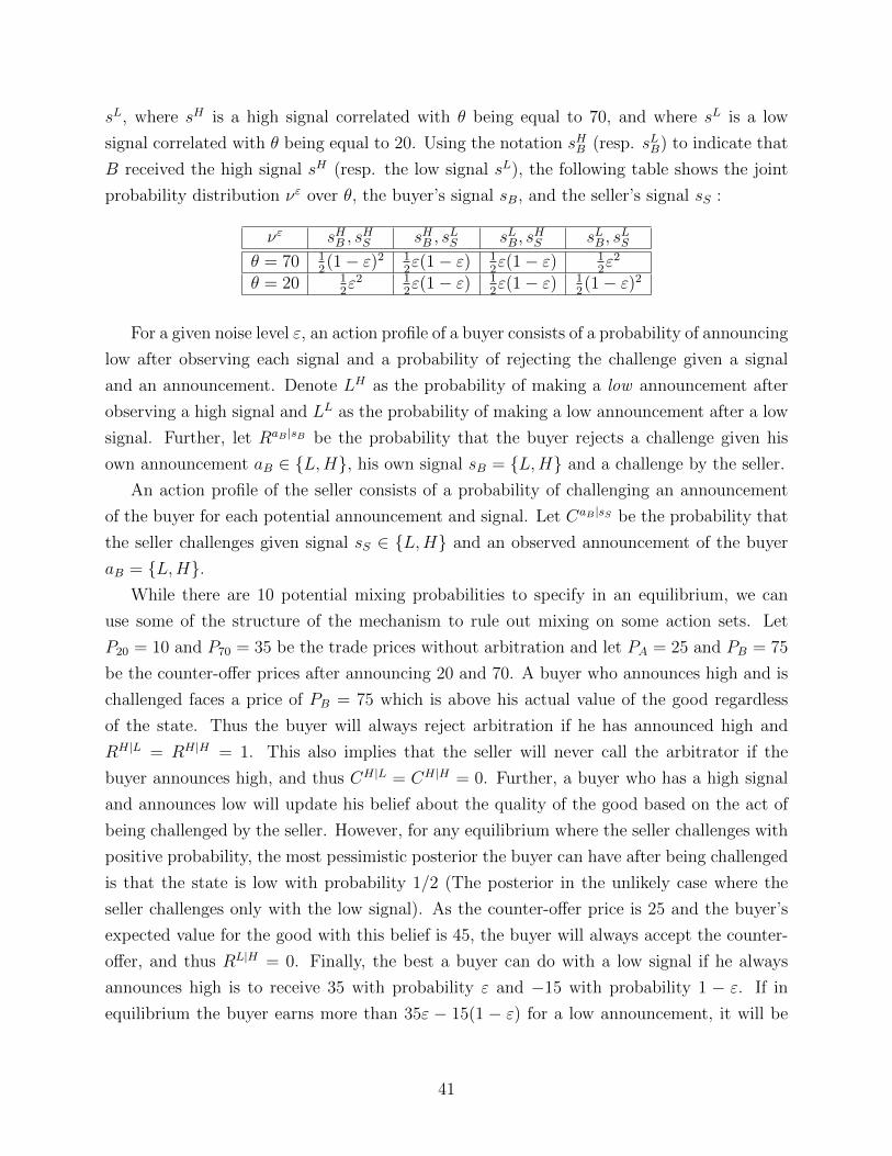
sL, where sH is a high signal correlated with θ being equal to 70, and where sL is a low
signal correlated with θ being equal to 20. Using the notation sHB (resp. sLB) to indicate that
B received the high signal sH (resp. the low signal sL), the following table shows the joint
probability distribution νε over θ, the buyer’s signal sB, and the seller’s signal sS :
νε sHB , sHS sHB , s
LS sLB, s
HS sLB, s
LS
θ = 70 12(1− ε)2 1
2ε(1− ε) 1
2ε(1− ε) 1
2ε2
θ = 20 12ε2 1
2ε(1− ε) 1
2ε(1− ε) 1
2(1− ε)2
For a given noise level ε, an action profile of a buyer consists of a probability of announcing
low after observing each signal and a probability of rejecting the challenge given a signal
and an announcement. Denote LH as the probability of making a low announcement after
observing a high signal and LL as the probability of making a low announcement after a low
signal. Further, let RaB |sB be the probability that the buyer rejects a challenge given his
own announcement aB ∈ {L,H}, his own signal sB = {L,H} and a challenge by the seller.
An action profile of the seller consists of a probability of challenging an announcement
of the buyer for each potential announcement and signal. Let CaB |sS be the probability that
the seller challenges given signal sS ∈ {L,H} and an observed announcement of the buyer
aB = {L,H}.While there are 10 potential mixing probabilities to specify in an equilibrium, we can
use some of the structure of the mechanism to rule out mixing on some action sets. Let
P20 = 10 and P70 = 35 be the trade prices without arbitration and let PA = 25 and PB = 75
be the counter-offer prices after announcing 20 and 70. A buyer who announces high and is
challenged faces a price of PB = 75 which is above his actual value of the good regardless
of the state. Thus the buyer will always reject arbitration if he has announced high and
RH|L = RH|H = 1. This also implies that the seller will never call the arbitrator if the
buyer announces high, and thus CH|L = CH|H = 0. Further, a buyer who has a high signal
and announces low will update his belief about the quality of the good based on the act of
being challenged by the seller. However, for any equilibrium where the seller challenges with
positive probability, the most pessimistic posterior the buyer can have after being challenged
is that the state is low with probability 1/2 (The posterior in the unlikely case where the
seller challenges only with the low signal). As the counter-offer price is 25 and the buyer’s
expected value for the good with this belief is 45, the buyer will always accept the counter-
offer, and thus RL|H = 0. Finally, the best a buyer can do with a low signal if he always
announces high is to receive 35 with probability ε and −15 with probability 1 − ε. If in
equilibrium the buyer earns more than 35ε − 15(1 − ε) for a low announcement, it will be
41
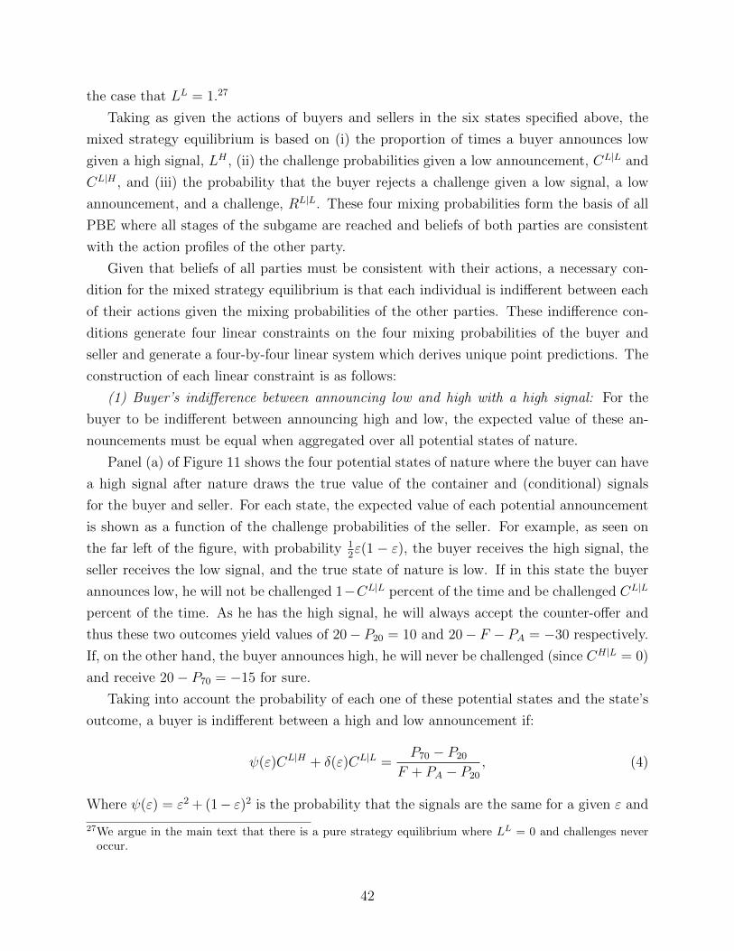
the case that LL = 1.27
Taking as given the actions of buyers and sellers in the six states specified above, the
mixed strategy equilibrium is based on (i) the proportion of times a buyer announces low
given a high signal, LH , (ii) the challenge probabilities given a low announcement, CL|L and
CL|H , and (iii) the probability that the buyer rejects a challenge given a low signal, a low
announcement, and a challenge, RL|L. These four mixing probabilities form the basis of all
PBE where all stages of the subgame are reached and beliefs of both parties are consistent
with the action profiles of the other party.
Given that beliefs of all parties must be consistent with their actions, a necessary con-
dition for the mixed strategy equilibrium is that each individual is indifferent between each
of their actions given the mixing probabilities of the other parties. These indifference con-
ditions generate four linear constraints on the four mixing probabilities of the buyer and
seller and generate a four-by-four linear system which derives unique point predictions. The
construction of each linear constraint is as follows:
(1) Buyer’s indifference between announcing low and high with a high signal: For the
buyer to be indifferent between announcing high and low, the expected value of these an-
nouncements must be equal when aggregated over all potential states of nature.
Panel (a) of Figure 11 shows the four potential states of nature where the buyer can have
a high signal after nature draws the true value of the container and (conditional) signals
for the buyer and seller. For each state, the expected value of each potential announcement
is shown as a function of the challenge probabilities of the seller. For example, as seen on
the far left of the figure, with probability 12ε(1 − ε), the buyer receives the high signal, the
seller receives the low signal, and the true state of nature is low. If in this state the buyer
announces low, he will not be challenged 1−CL|L percent of the time and be challenged CL|L
percent of the time. As he has the high signal, he will always accept the counter-offer and
thus these two outcomes yield values of 20− P20 = 10 and 20− F − PA = −30 respectively.
If, on the other hand, the buyer announces high, he will never be challenged (since CH|L = 0)
and receive 20− P70 = −15 for sure.
Taking into account the probability of each one of these potential states and the state’s
outcome, a buyer is indifferent between a high and low announcement if:
ψ(ε)CL|H + δ(ε)CL|L =P70 − P20
F + PA − P20
, (4)
Where ψ(ε) = ε2 + (1− ε)2 is the probability that the signals are the same for a given ε and
27We argue in the main text that there is a pure strategy equilibrium where LL = 0 and challenges neveroccur.
42
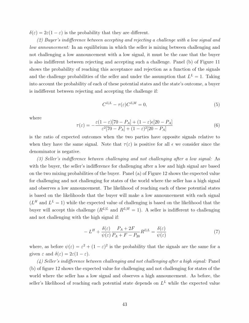
δ(ε) = 2ε(1− ε) is the probability that they are different.
(2) Buyer’s indifference between accepting and rejecting a challenge with a low signal and
low announcement: In an equilibrium in which the seller is mixing between challenging and
not challenging a low announcement with a low signal, it must be the case that the buyer
is also indifferent between rejecting and accepting such a challenge. Panel (b) of Figure 11
shows the probability of reaching this acceptance and rejection as a function of the signals
and the challenge probabilities of the seller and under the assumption that LL = 1. Taking
into account the probability of each of these potential states and the state’s outcome, a buyer
is indifferent between rejecting and accepting the challenge if:
CL|L − τ(ε)CL|H = 0, (5)
where
τ(ε) = −ε(1− ε)[70− PA] + (1− ε)ε[20− PA]
ε2[70− PA] + (1− ε)2[20− PA](6)
is the ratio of expected outcomes when the two parties have opposite signals relative to
when they have the same signal. Note that τ(ε) is positive for all ε we consider since the
denominator is negative.
(3) Seller’s indifference between challenging and not challenging after a low signal: As
with the buyer, the seller’s indifference for challenging after a low and high signal are based
on the two mixing probabilities of the buyer. Panel (a) of Figure 12 shows the expected value
for challenging and not challenging for states of the world where the seller has a high signal
and observes a low announcement. The likelihood of reaching each of these potential states
is based on the likelihoods that the buyer will make a low announcement with each signal
(LH and LL = 1) while the expected value of challenging is based on the likelihood that the
buyer will accept this challenge (RL|L and RL|H = 1). A seller is indifferent to challenging
and not challenging with the high signal if:
− LH +δ(ε)
ψ(ε)
PA + 2F
PA + F − P20
RL|L =δ(ε)
ψ(ε)(7)
where, as before ψ(ε) = ε2 + (1 − ε)2 is the probability that the signals are the same for a
given ε and δ(ε) = 2ε(1− ε).(4) Seller’s indifference between challenging and not challenging after a high signal: Panel
(b) of figure 12 shows the expected value for challenging and not challenging for states of the
world where the seller has a low signal and observes a high announcement. As before, the
seller’s likelihood of reaching each potential state depends on LL while the expected value
43
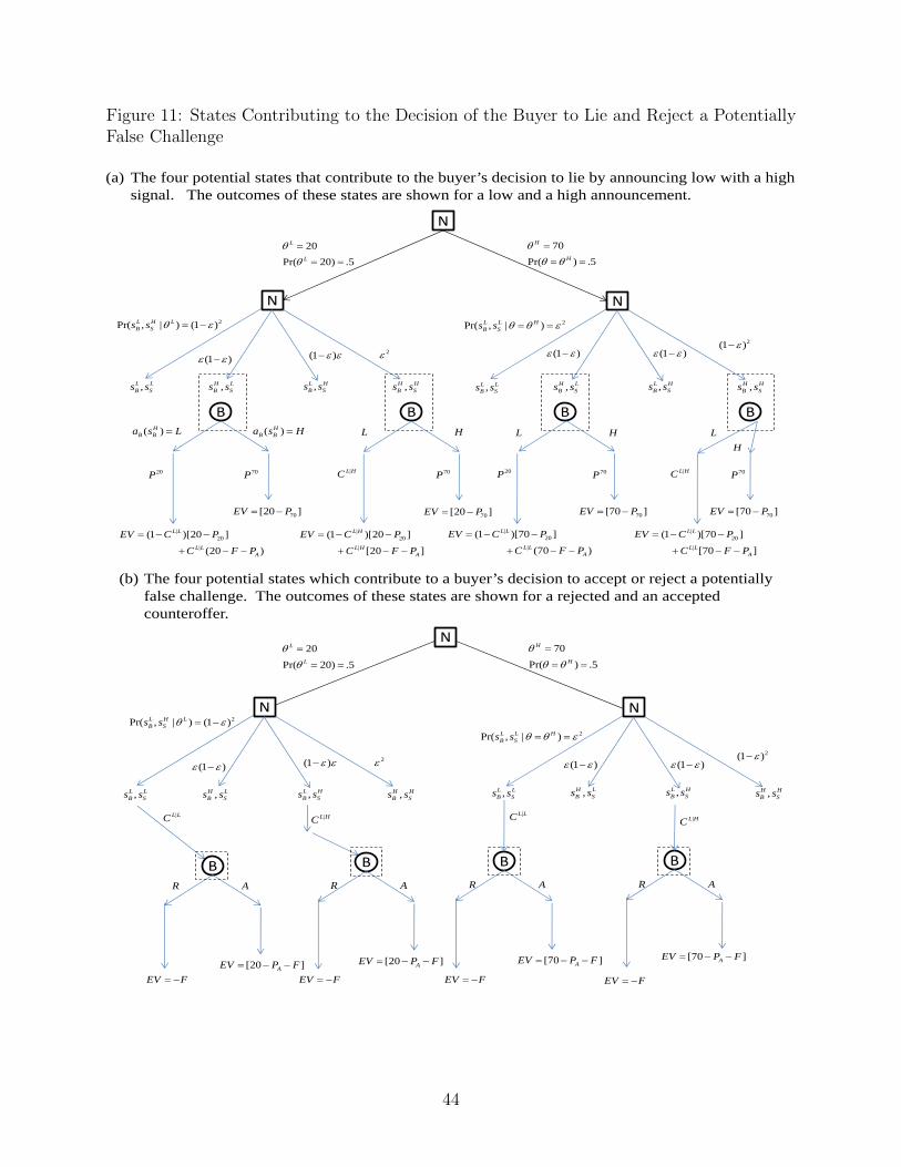
Figure 11: States Contributing to the Decision of the Buyer to Lie and Reject a PotentiallyFalse Challenge
N
N N
|L LC
BR A
B B B
EV F
[20 ]AEV P F
|L HC
R A R A R A
EV F
[20 ]AEV P F
EV F
[70 ]AEV P F
EV F
[70 ]AEV P F
20
Pr( 20) .5
L
L
70
Pr( ) .5
H
H
,L LB Ss s
2Pr( , | ) (1 ) L H LB Ss s
(1 )
,H LB Ss s
(1 )
,L HB Ss s ,H H
B Ss s
2
,L LB Ss s
2Pr( , | ) L L HB Ss s
(1 ) (1 ) 2(1 )
,H LB Ss s ,L H
B Ss s ,H HB Ss s
|L LC |L HC
N
20
Pr( 20) .5
L
L
70
Pr( ) .5
H
H
N
,L LB Ss s
2Pr( , | ) (1 ) L H LB Ss s
(1 )
,H LB Ss s
(1 )
,L HB Ss s ,H H
B Ss s
2
N
,L LB Ss s
2Pr( , | ) L L HB Ss s
(1 ) (1 ) 2(1 )
20P
|20
|
(1 )[20 ]
[20 ]
L H
L HA
EV C P
C F P
|20
|
(1 )[20 ]
(20 )
L L
L LA
EV C P
C F P
|20
|
(1 )[70 ]
[70 ]
L L
L LA
EV C P
C F P
B B B B( ) H
B Ba s L ( ) HB Ba s H
70P
70[20 ]EV P
70P
70[20 ]EV P
20P
|20
|
(1 )[70 ]
(70 )
L L
L LA
EV C P
C F P
70P
70[70 ]EV P
70P
70[70 ]EV P
,H LB Ss s ,L H
B Ss s ,H HB Ss s
L H L H L
H
|L HC |L HC
(a) The four potential states that contribute to the buyer’s decision to lie by announcing low with a high signal. The outcomes of these states are shown for a low and a high announcement.
(b) The four potential states which contribute to a buyer’s decision to accept or reject a potentially false challenge. The outcomes of these states are shown for a rejected and an accepted counteroffer.
44
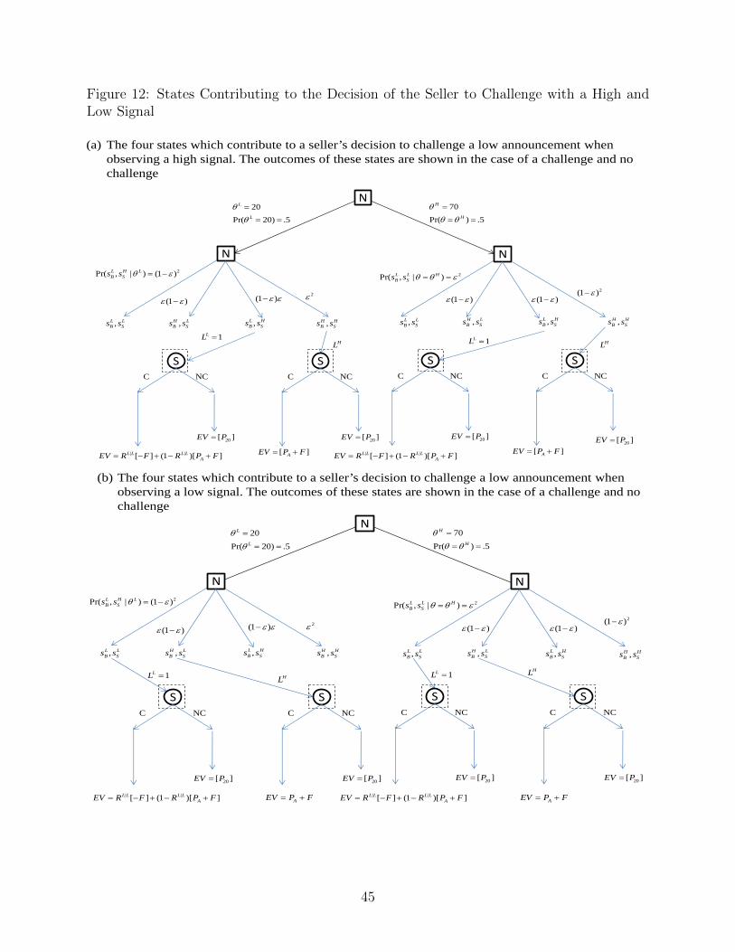
Figure 12: States Contributing to the Decision of the Seller to Challenge with a High andLow Signal
N
N N
1LL HL1LL
HL
SC NC
SC NC
SC NC
SC NC
| |[ ] (1 )[ ] L L L LAEV R F R P F
20[ ]EV P 20[ ]EV P 20[ ]EV P 20[ ]EV P
| |[ ] (1 )[ ] L L L LAEV R F R P FAEV P F AEV P F
20
Pr( 20) .5
L
L
70
Pr( ) .5
H
H
,L LB Ss s
2Pr( , | ) (1 ) L H LB Ss s
(1 )
,H LB Ss s
(1 )
,L HB Ss s ,H H
B Ss s
2
,L LB Ss s
2Pr( , | ) L L HB Ss s
(1 ) (1 ) 2(1 )
,H LB Ss s ,L H
B Ss s ,H HB Ss s
N
N N
HL1LL
SC NC
20[ ]EV P
SC NC
[ ]AEV P F
20[ ]EV P
SC NC
20[ ]EV P
SC NC
[ ]AEV P F 20[ ]EV P
| |[ ] (1 )[ ] L L L LAEV R F R P F | |[ ] (1 )[ ] L L L L
AEV R F R P F
20
Pr( 20) .5
L
L
70
Pr( ) .5
H
H
,L LB Ss s
2Pr( , | ) (1 ) L H LB Ss s
(1 )
,H LB Ss s
(1 )
,L HB Ss s ,H H
B Ss s
2
,L LB Ss s
2Pr( , | ) L L HB Ss s
(1 ) (1 ) 2(1 )
,H LB Ss s ,L H
B Ss s ,H HB Ss s
HL1LL
(a) The four states which contribute to a seller’s decision to challenge a low announcement when observing a high signal. The outcomes of these states are shown in the case of a challenge and no challenge
(b) The four states which contribute to a seller’s decision to challenge a low announcement when observing a low signal. The outcomes of these states are shown in the case of a challenge and no challenge
45
within these nodes depends on RL|L. A seller is indifferent to lying and not lying if:
− LH +ψ(ε)
δ(ε)
PA + 2F
PA + F − P20
RL|L =ψ(ε)
δ(ε). (8)
Note that this is identical to the seller’s indifference condition for challenging with the low
signal except that the ratio of states is inverted.
Given the four indifference conditions, the point predictions of the model come from
solving the four-by-four system of simultaneous equations. The solution to this system is as
follows:
Result 7 With selfish agents, the mixed strategy equilibrium with ε = .05 is LH = 0, RL|L =
.53333, CL|H = .66, and CL|L = .285. The mixed strategy equilibrium with ε = .1 is LH = 0,
RL|L = .53333, CL|H = .625, and CL|L = .625.
The surprising restriction that LH = 0 is due to the fact that the seller must be indifferent
to mixing in the case of a high and low signal.
Appendix B: Mechanism used to elicit incentive com-
patible beliefs
In the follow-up treatment with incentive compatible beliefs, we use the following belief
elicitation game based on a mechanism developed by Karni (2009). For each potential
combination of announcement and signal, buyers are asked to submit a belief, b, between 0
and 100 corresponding to the percentage chance that the seller will call in the arbitrator.
A random number c ∈ [0, 100] is then drawn by the computer which corresponds to the
“computer’s percentage chance of calling in the arbitrator.”
At the end of the experiment, one of the periods is randomly selected for payment.
Using an eight-sided dice, the main experiment is paid 50% of the time while each of the
four potential beliefs are paid 12.5% of the time. If a belief elicitation game is selected, the
belief elicitation game is resolved as follows. If b ≤ c the buyer is matched with the seller
and his outcome is based on the arbitration decision of the seller. If the seller does not
call the arbitrator, the buyer receives $20. If, however, the seller calls the arbitrator, the
buyer receives $0. If b > c, the buyer is matched to the computer. The computer calls the
arbitrator with probability c/100 and thus the buyer receives $20 with probability 1−(c/100)
and $0 otherwise.
The mechanism is similar to the Becker, DeGroot, Marshack (1964) mechanism and is
shown by Karni (2009) to induce truthful reporting of beliefs for rational agents with any
46
von Neumann-Morgenstern utility function. Further, as individuals are paid only for the
main experiment or the bonus game, there is no concerns about hedging. The mechanism
and payment scheme are thus robust to heterogeneity in risk aversion and are incentive
compatible.
As the belief elicitation mechanism is relatively complex, we provide extensive training
with the mechanism before the start of the experiment. Buyers receive both written and oral
instructions about the mechanism, which include a series of examples that make clear that
under reporting or over reporting beliefs can lead to worse outcomes. Subjects are also told
explicitly that it is best to write down their true belief. Following the instructions, subjects
are also given a series of quiz questions about the elicitation mechanism where they must
calculate various potential outcomes for truthfully reported and misreported beliefs.
47