riemann surfaces; s. k. donaldson
TRANSCRIPT

Riemann Surfaces
S. K. Donaldson
December 2, 2004

2

Contents
I Preliminaries 7
1 Holomorphic functions 9
1.1 Simple examples; algebraic functions . . . . . . . . . . . . . . 9
1.2 Analytic continuation; differential equations . . . . . . . . . . 12
2 Surface Topology 17
2.1 Classification of surfaces . . . . . . . . . . . . . . . . . . . . . 17
2.2 Discussion: the mapping class group . . . . . . . . . . . . . . 22
II Basic Theory 25
3 Basic definitions 27
3.1 Riemann surfaces and holomorphic maps . . . . . . . . . . . . 27
3.2 Examples . . . . . . . . . . . . . . . . . . . . . . . . . . . . . 30
3.2.1 . . . . . . . . . . . . . . . . . . . . . . . . . . . . . . . 30
3.2.2 Algebraic curves . . . . . . . . . . . . . . . . . . . . . 31
3.2.3 Quotients. . . . . . . . . . . . . . . . . . . . . . . . . 35
4 Maps between Riemann surfaces 37
4.1 General properties . . . . . . . . . . . . . . . . . . . . . . . . 37
4.2 Monodromy and the Riemann Existence Theorem . . . . . . . 41
4.2.1 Digression in algebraic topology . . . . . . . . . . . . . 41
4.2.2 Monodromy of covering maps . . . . . . . . . . . . . . 43
4.2.3 Compactifying algebraic curves . . . . . . . . . . . . . 46
4.2.4 The Riemann surface of a holomorphic function . . . . 48
3

4 CONTENTS
5 Calculus on surfaces 515.1 Smooth surfaces . . . . . . . . . . . . . . . . . . . . . . . . . . 51
5.1.1 Cotangent spaces and 1-forms . . . . . . . . . . . . . . 515.1.2 2-forms and integration . . . . . . . . . . . . . . . . . . 55
5.2 de Rham cohomology . . . . . . . . . . . . . . . . . . . . . . . 625.2.1 Definition and examples . . . . . . . . . . . . . . . . . 625.2.2 Cohomology with compact support and Poincare duality 65
5.3 Calculus on Riemann surfaces . . . . . . . . . . . . . . . . . . 695.3.1 Decomposition of the 1-forms . . . . . . . . . . . . . . 695.3.2 The Laplace operator and harmonic functions . . . . . 725.3.3 The Dirichlet norm . . . . . . . . . . . . . . . . . . . . 73
6 Elliptic functions and integrals 776.0.4 Elliptic integrals . . . . . . . . . . . . . . . . . . . . . 776.0.5 The Weierstrasse function . . . . . . . . . . . . . . . . 82
7 Applications of the Euler characteristic 857.1 The Euler characteristic and meromorphic forms . . . . . . . . 85
7.1.1 Topology . . . . . . . . . . . . . . . . . . . . . . . . . . 857.1.2 Meromorphic forms . . . . . . . . . . . . . . . . . . . . 87
7.2 Applications . . . . . . . . . . . . . . . . . . . . . . . . . . . . 887.2.1 The Riemann-Hurwitz formula . . . . . . . . . . . . . . 887.2.2 The degree-genus formula . . . . . . . . . . . . . . . . 897.2.3 Real structures and Harnack’s bound . . . . . . . . . . 907.2.4 Modular curves . . . . . . . . . . . . . . . . . . . . . . 93
III Deeper Theory 95
8 Meromorphic functions and the Main Theorem for compactRiemann surfaces 978.1 Consequences of the main theorem . . . . . . . . . . . . . . . 99
9 Proof of the Main Theorem 1039.1 Discussion and motivation . . . . . . . . . . . . . . . . . . . . 1039.2 The Riesz representation theorem . . . . . . . . . . . . . . . . 1069.3 The heart of the proof . . . . . . . . . . . . . . . . . . . . . . 1089.4 Weyl’s Lemma . . . . . . . . . . . . . . . . . . . . . . . . . . . 112

CONTENTS 5
10 The Uniformisation Theorem 11710.1 Statement . . . . . . . . . . . . . . . . . . . . . . . . . . . . . 11710.2 Proof of the analogue of the Main Theorem . . . . . . . . . . 120
10.2.1 Set-up . . . . . . . . . . . . . . . . . . . . . . . . . . . 12010.2.2 Classification of behaviour at infinity . . . . . . . . . . 12210.2.3 The main argument . . . . . . . . . . . . . . . . . . . . 125

6 CONTENTS

Part I
Preliminaries
7


Chapter 1
Holomorphic functions
1.1 Simple examples; algebraic functions
This is an introductory Chapter in which we recall some examples of holo-morphic functions in complex analysis. We emphasise the idea of “analyticcontinuation” which is a fundamental motivation for Riemann surface theory.
One naturally encounters holomorphic functions in various ways. Oneway is through power series, say f(z) =
∑anz
n. It often happens that afunction which is initially defined on some open set U ⊂ C turns out to havenatural extensions to larger open sets. for example the power series
f(z) = 1 + z + z2 + z3 + . . .
converges only for |z| < 1, but writing f(z) = 1/(1 − z) we see that thefunction actually extends to C \ 1. A more subtle example is the Gammafunction. For <(z) > 0 we write
Γ(z) =∫ ∞
0tz−1e−tdt.
The integral is convergent and defines a holomorphic function of z on thishalf-plane. Integration by parts shows that
Γ(n) = (n− 1)!
if n is a positive integer. It is clear that Γ(z) tends to infinity as z tends to0 but let us examine this more carefully by writing
Γ(z) =∫ 1
0tz−1e−tdt+
∫ ∞1
tz−1e−tdt.
9

10 CHAPTER 1. HOLOMORPHIC FUNCTIONS
The second integral is defined for all z, and holomorphic in z. We write thefirst integral as ∫ 1
0tz−1(et − 1)dt+
∫ 1
0tz−1dt.
Now the term ∫ 1
0tz−1(et − 1)dt
is defined, and holomorphic in z, for <(z) > −1. The other integral we canevaluate explicitly: ∫ 1
0tz−1dt =
1
z.
So we conclude that, for <(z) > 0,
Γ(z) =1
z+ Γ1(z)
say, where Γ1 extends to a holomorphic function on the larger half-planez : <(z) > −1. So Γ has a meromorphic extension to the larger half-plane.Repeating the procedure, by considering
e−t − (1− t+t2
2!− t3
3!+ . . .+
(−t)kk!
),
we get a meromorphic extension to <(z) > −(k+1), and thence to the wholeof C.
Exercise. Show that Γ has a simple pole at the point z = −k for positiveintegers k, with residue (−1)k/k!.
It often happens that when extending a function one encounters “multiplevalued functions”. For example
f(z) = 1 +z
2− z2
222!+
3z3
233!− 5.3z5
244!+ . . . ,
is a perfectly good holomorphic function on the disc |z| < 1 which we recog-nise as
√1 + z. This cannot be extended holomorphicaly to z = −1 but,
more, if we try to extend the function to C \ −1 we find that going oncearound the origin the function switches to the other branch of the squareroot. Particularly important examples of this phenomena occur for “alge-braic functions”.

1.1. SIMPLE EXAMPLES; ALGEBRAIC FUNCTIONS 11
Let P (z, w) be a polynomial in two complex variables. We want to thinkof the equation P (z, w) = 0 as defining w “implicitly” as a function of z.For example if P (z, w) = w2 − (1 + z) then we would get the function w =√
1 + z above. Or if P (z, w) = z3 + w2 − 1 we would get the functionw =
√1− z3. Of course this does not make sense precisely because of the
problem of multiple values. The next theorem, which will be fundamentallater, expresses precisely the way in which such functions are defined.
First, some notation. Let X ⊂ C2 be the set of points (z, w) withP (z, w) = 0. Second, we define the partial derivatives
∂P
∂z,∂P
∂w,
in the obvious way. They are again polynomial functions of the two variablesz, w.
Theorem 1 Suppose (z0, w0) is a point in X and ∂P∂w
does not vanish at(z0, w0). Then there is a disc D1 centred at z0 in C and a disc D2 centred atw0 and a holomorphic map φ : D1 → D2 with φ(z0) = w0 such that
X ∩ (D1 ×D2) = (z, φ(z)) : z ∈ D1.The reader will recognise the set in the statement as the “graph” of the
map φ. Essentially the theorem says that w = φ(z) gives the unique localsolution to the equation P (z, w) = 0, where local means close to (z0, w0).
To prove the Theorem, recall that if f is a holomorphic function on anopen set containing the closure of a disc D which does not vanish on theboundary ∂D then the number of solutions of the equation f(w) = 0 in D,counted with multiplicity, is given by the contour integral
1
2πi
∫∂D
f ′(w)
f(w)dw.
If there is only one solution, w1, it is given by another contour integral
w1 =1
2πi
∫∂D
wf ′(w)
f(w)dw.
We apply these formulae to the family of functions of the variable w: fz(w) =P (z, w), where we regard z as a parameter. First take z = z0. Then thehypothesis that ∂P
∂w6= 0 means that f ′z0 does not vanish at w0. Thus we can

12 CHAPTER 1. HOLOMORPHIC FUNCTIONS
find a small disc D2 centred at w0 so that fz0 has no other zeros in the closureof D2. Since the boundary of D2 is compact there is some δ > 0 such that|fz0 | > 2δ on ∂D2. By continuity, this means that if z is sufficiently close toz0 we still have |fz| > δ, say, on ∂D2. Thus we can apply the formula abovefor the number of roots of the equation fz(w) = 0. When z = z0 this mustbe 1 so, by continuity, the same is true for z close to z0. Then we define φ(z)to be this unique root. The second formula shows that
φ(z) =∫∂D2
w
P
∂P
∂wdw,
which is clearly holomorphic in the variable z. This completes the proof.
1.2 Analytic continuation; differential equa-
tions
Next we want to give a precise meaning to possibly many-valued extensionsof a holomorphic function.
Definition 1 Let φ be a holomorphic function defined on a neighbourhoodof a point z0 ∈ C. Let γ : [0, 1] → C be a continuous map with γ(0) = z0.An analytic continuation of φ along γ consists of a family of holomorphicfunctions φt, for t ∈ [0, 1], where φt is defined on a neighbourhood Ut of γ(t)such that
• φ0 = φ on some neighbourhood of z0;
• for each t0 ∈ [0, 1] there is a δt0 > 0 such that if |t− t0| < δt0 the func-tions φt and φt0 are equal on their their common domain of definitionUt ∩ Ut0.
For example suppose z0 = 0 and φ is the function defined by the powerseries above, giving a branch of
√1 + z. Let γ be the path which traces out
the circle centred at −1γ(t) = −1 + e2πit.
The the reader will see how to construct an analytic continuation of φ alongthis path with φ1 equal to the other branch of the square root,
φ1 = −φ,

1.2. ANALYTIC CONTINUATION; DIFFERENTIAL EQUATIONS 13
on a suitable neighbourhood of 0.Alongside the algebraic equations discussed above, another very impor-
tant way in which holomorphic functions arise is as solutions to differentialequations. Of course the simplest example here is the differential equation
du
dz= g,
where g is a given function, whose solution is the indefinite integral of g andis given by a contour integral. We know that we may again encounter manyvalued functions, for example when g is the function 1/z. In our currentlanguage, the contour integral along a (smooth) path γ furnishes an analyticcontinuation of a local solution along γ.
We will consider second order linear, homogeneous equations of the form;
u′′ + Pu′ +Qu = 0,
where P and Q are given functions of z and u is to be found. Supposefirst that P and Q are holomorphic near z = 0. So they have power seriesexpansions
P (z) =∑
pnzn , Q(z) =
∑qnz
n,
valid in some common region |z| < R. We seek a solution to the equation inthe form u(z) =
∑unz
n. Equating terms we get, for each n ≥ 0,
(n+ 2)(n+ 1)un+2 +∑i≥0
(n+ 1− i)piun+1−i +∑j≥0
qjun−j = 0.
Both the sums are finite and only contain terms ui for i < n+2, so this givesrecursion formula. Given any choice of u0, u1 there is a unique way to defineall the ui satisfying the equations.
Exercise Show that the power series∑unz
n converges for |z| < R.We conclude that the solutions of our equation on the disc |z| < R form
a 2-dimensional complex vector space.Now suppose that P,Q are holomorphic on some open set Ω ⊂ C and let
γ : [0, 1]→ Ω be a path in Ω.
Proposition 1 If u is a solution to the equation (*) on a neighbourhood ofγ(0) then u has an analytic continuation along γ, through solutions of theequation

14 CHAPTER 1. HOLOMORPHIC FUNCTIONS
We leave the proof as an exercise. (In fact one can generalise the resultto the case when P,Q are themselves defined initially in a neighbourhood ofγ(0) and have analytic continuations along γ.)
This leads to the notion of the “monodromy” of solutions to a differentialequation. Suppose γ is a loop in Ω, with γ(0) = γ(1). Let u1, u2 be a basis forthe solutions of the differential equation on a small neighbourhood of γ(0).Analytic continuation of u1, u2 along γ yields another pair of solutionsu1, u2
say. these are linear combinations of the original pair
u1 = au1 + bu2, u2 = cu1 + du2.
In more invariant language, let V be the two dimensional vector space oflocal solutions, then analytic continuation along γ gives a linear map
Mγ : V → V.
Interesting examples arise when the complement of Ω is a discrete subsetof C and P,Q are meromorphic.
Definition 2 A point z0 ∈ C is a regular singular point of the equationu′′ + Pu′ +Qu = 0 if P has at worst a simple pole at z0 and Q has at worsta double pole.
Consider a model case,
u′′ +A
zu′ +
B
z2u = 0,
where A,B are complex constants. We try a solution u = zα defined on acut plane, say. This satisfies the equation if
α(α− 1) + Aα +B = 0.
If this quadratic equation (the indicial equation) has two distinct roots α1, α2
we get two solutions to our equation zα1 , zα2 in the cut plane. If there is adouble root α, the second solution is zα log z. The general case is similar
Proposition 2 If P (z) = Az
+ P0(z) and Q(z) = Bz2 + C
z+ Q0(z) where
P0, Q0 are holomorphic near 0 and if the indicial equation has roots α1, α2
with α1 − α2 /∈ Z then there are solutions
u1(z) = zα1w1(z) , u2(z) = zα2w2(z),
to the equation u′′ + Pu′ +Qu = 0 where w1, w2 are holomorphic in a neigh-bourhood of 0.

1.2. ANALYTIC CONTINUATION; DIFFERENTIAL EQUATIONS 15
The proof goes by power series expansion, as before. If α1 − α2 ∈ Z thesecond solution may involve log terms. Expressed in terms of monodromy, ifz0 is a regular single point of the equation u′′ + Pu′ +Q = 0 and γ is a looparound z0 then in the case when α1−α2 /∈ Z the monodromy around γ is (ina suitable basis) the diagonal matrix with entries e2πiα1 , e2πiα2 . In the othercase we may get a nontrivial Jordan form.
A very important example, which we will return to later, is the hyperge-ometric equation:
z(1− z)u′′ + (c− (a+ b+ 1)z)u′ − abu = 0,
which has regular singular points at 0, 1. (It also has a regular single point“at infinity” as we will explain later.) Here a, b, c are fixed parameters.
Exercise Show that the indicial equation at z = 0 has roots 0, c and thatthe solution corresponding to the root 0 is the hypergeometric function
F (z) = 1 +ab
cz+
a(a+ 1)b(b+ 1)
c(c+ 1)2!z2 +
a(a+ 1)a+ 2)b(b+ 1)(b+ 2)
c(c+ 1)(c+ 2)3!z3 + . . . ,
in |z| < 1.

16 CHAPTER 1. HOLOMORPHIC FUNCTIONS

Chapter 2
Surface Topology
2.1 Classification of surfaces
In this second introductory chapter we change direction completely. Wediscuss the topological classification of surfaces, and outline one approachto a proof. Our treatment here is almost entirely informal; we do not evendefine precisely what we mean by a “surface”. (Definitions will be found inthe following Chapter.) However it is not in fact too hard to turn our informalaccount into a precise proof. The reasons for including this material here are,first, that it gives a counterweight to the previous chapter: the two togetherillustrating two themes—complex analysis and topology—which run throughthe subject of Riemann surfaces; and, second, that we are able to introducesome more advanced ideas that will be taken up later in the book.
The statement of the clasification of closed surfaces is probably well-known to many readers. We write down two families of surfaces Σg,Ξh forintegers g ≥ 0, h ≥ 1.
The surface Σ0 is the 2-sphere S2. The surface Σ1 is the 2-torus T 2. Forg ≥ 2 we define the surface Σg by taking the “connected sum” of g copiesof the torus. In general if X and Y are (connected) surfaces the connectedsum X]Y is a surface constructed as follows. We choose small discs DX in Xand DY in Y and cut them out to get a pair of “surfaces-with-boundaries”,coresponding to the circle boundaries of DX and DY . Then we glue theseboundary circles together to form X]Y . [DIAGRAM 1]
One can show that this resulting surface is (up to natural equivalence)
17
18 CHAPTER 2. SURFACE TOPOLOGY
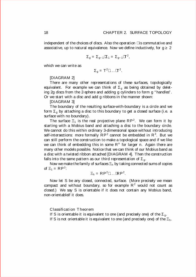
independent of the choices of discs. Also the operation ] is commutative andassociative, up to natural equivalence. Now we define inductively, for g ≥ 2
Σg = Σg−1]Σ1 = Σg−1]T2,
which we can write as
Σg = T 2] . . . ]T 2.
[DIAGRAM 2]There are many other representations of these surfaces, topologically
equivalent. For example we can think of Σg as being obtained by delet-ing 2g discs from the 2-sphere and adding g cylinders to form g “handles”.Or we start with a disc and add g ribbons in the manner shown:
[DIAGRAM 3]The boundary of the resulting surface-with-boundary is a circle and we
form Σg by attaching a disc to this boundary to get a closed surface (i.e. asurface with no boundary).
The surface Ξ1 is the real projective plane RP 2. We can form it bystarting with a Mobius band and attaching a disc to the boundary circle.We cannot do this within ordinary 3-dimensional space without introducingself-intersections: more formally RP 2 cannot be embedded in R3. But wecan still perform the construction to make a topological space and if we likewe can think of embedding this in some Rn for larger n. Again there aremany other models possible. Notice that we can think of our Mobius band asa disc with a twisted ribbon attached [DIAGRAM 4]. Then the constructionfalls into the same pattern as our third representation of Σg.
Now we make the family of surfaces Ξh by taking connected sums of copiesof Ξ1 = RP 2:
Ξh = RP 2] . . . ]RP 2.
Now let S be any closed, connected, surface. (More precisely we meancompact and without boundary, so for example R2 would not count asclosed.) We say S is orientable if it does not contain any Mobius band,non-orientableif it does.
Classification TheoremIf S is orientable it is equivalent to one (and precisely one) of the Σg.If S is not orientable it is equivalent to one (and precisely one) of the Ξh.

2.1. CLASSIFICATION OF SURFACES 19
(We emphasise again that this statement has quite a different status fromthe other “Theorems” in this book, since we have not even defined the termsprecisely.)
To see an example of this, consider the “Klein bottle” K. This can bepictured in R3 as shown in [DIAGRAM 5], except that there is a circle ofself-intersection. So we should think of pushing the handle of the surface intoa fourth dimension where it passes through the “side”, just as we can take acurve in the plane as pictured in [DIAGRAM 6] and remove the intersectionpoint by lifting one branch into three dimensions.
Now it is true but perhaps not immediately obvious, that K is equivalentto Ξ2. To see this cut the picture in Diagram 5 down the vertical plane ofsymmetry. Then you can see that K is formed by gluing two Mobius bandsalong their boundaries. By definition of the connected sum this shows thatK = RP 2]RP 2, since the complement of a disc in RP 2 is a Mobius band.
Now we will outline a proof of the classification theorem. The proofuses ideas that (when developed in a rigorous way of course), go under thename of “Morse Theory”. A detailed technical account is given in the bookDifferential Topology by Hirsch. The idea is that, given our closed surface S,we choose a typical real valued function on S. Here “typical” means, moreprecisely, that f is what is called a Morse function. What this requires is thatif we introduce a choice of gradient vector field of f on S then there are onlya finite number of points Pi, called critical points, in S where v vanishes, andnear any of one of these points Pi we can parametrise the surface by two realnumbers u, v such that the function is given by one of three local models:
• u2 + v2 + constant.
• u2 − v2 + constant.
• −u2 − v2 + constant.
The critical point Pi is said to have index 0, 1 or 2 respectively in these threecases.
For example if S is a typical surface in R3 we can take the functionf to be the restriction of the z co-ordinate (say): the “height” function

20 CHAPTER 2. SURFACE TOPOLOGY
on S. The vector field v is the projection of the unit vertical vector tothe tangent spaces of S and the critical points are the points where thetangent space is horizontal. The points of index 0 and 2 are local minima andmaxima respectively and the critical points of index 1 are “saddle points”.[DIAGRAM 8]
Now for each t ∈ R we can consider the subset St = x ∈ S : f(x) ≤ t.There are a finite number of special cases, the “critical values” f(Pi) wherePi is a critical point. If f is a sufficiently typical function then the valuesf(Pi) will all be different, so to each critical value we can associate just onecritical point. If t is not a critical value then St is a surface with boundary.Morover if t varies over an interval not containing any critical values thenthe surfaces-with boundaries St are equivalent for different parameters t inthe interval. To see this, if t1 < t2 and [t1, t2] does not contain any criticalvalue then one deforms St2 into St1 by pushing down the gradient vector fieldv. [DIAGRAM 9]
Now consider the exceptional case when t is a critical value, t0 say. Theset St0 is no longer a surface. However we can analyse the difference betweenSt+ε and St−ε for small positive ε. The crucial thing is that this analysis isconcentrated around the corresponding critical point, and the change is thesurface follws one of three standard local models, depending on the index.
Index 0 Near the critical point the St0±ε corresponds to u2 + v2 ≤ ±εwhich is empty in one case and a disc in the other case. In other words, St0+ε
is obtained from St0−ε by adding a disc as a new connected component.Index 2 This is the reverse of the index 0 case. The surface St0+ε is formed
by attaching a disc to a boundary component of St0−ε.index 1 This is a little more subtle. The local picture is to consider
u2 − v2 ≤ ±ε,as shown in [DIAGRAM 10]. This is equivalent to adding a strip to theboundary [DIAGRAM 11]. Thus St0+ε is formed by adding a strip to theboundary of St0−ε.
We can now see a stratgy to prove the Classification Theorem. Whatwe should do is to prove a more general theorem, classifying surfaces withboundary (not necessarily connected, and including the case of empty bound-ary). Suppose we have any class of model surfaces with boundary which isclosed under the three operations associated to index 0,1,2 critical pointsexplained above. Then it follows that our original closed surface S must liein this class, since it is obtained by a sequence of these operations.

2.1. CLASSIFICATION OF SURFACES 21
For r ≥ 0 let Σg,r be the surface with boundary (possibly empty) obtainedby removing r disjoint discs from Σg. Similarly for Ξh,r. Now we aim toprove that the class of disjoint unions of copies of the Σg,r and Ξh,r (for anycollection of g’s h’s and r’s) is closed under the three operations above. Thatis if X is in our class (a disjoint union of copies of Σg,r and Ξh,r and we obtainX ′ by performing of the operations then X ′ is also in our class. This doesrequire a little thought, and consideration of various cases.
Index 0 This is obvious, since Σ1,1 is the disc so we can include a new disccomponent in our class.
Index 2 Also obvious. We cap off some boundary component with a discturning some Σg,r into a Σg,r−1 or a Ξh,r into a Ξh,r−1.
Index 1 This requires more work. There are various cases to consider.Case 1. The ends of the attaching strip lie on different components of X.Case 2. The ends of the attaching strip lie on the same component of X.Now Case 2 subdivides intoCase 2(i) The ends of the strip lie on the same boundary component of a
component of X.Case 2(ii) The ends of the strip lie on the different boundary components
of one common component of X.Further, each of these cases 2(i), 2(ii) subdivide because there are two
ways we can make the attaching, diferring by a twist, in just the same fashionas when we form a Mobius band from a disc above. (The reader may like tothink through why we do not need to make this distinction in Case 1.)
Now let us get to work.Case 1. Let the relevant components of X be A and B say. Then we can
write A = A′ \ disc, B = B′ \ disc for some A′, B′ and \ disc means that theoperation of removing a disc, so of course the boundaries of the indicateddiscs contain the attaching regions. Then we can see that the manifold weget when we attach a strip is (A′]B′) \ disc. [DIAGRAM 12].
Case 2(i). Let the component of X to which we attach the strip beA = A′ \disc. Then in the untwisted case we get, after the strip attachment,A′ \ disc \ disc. [DIAGRAM 13]
In the twisted case we get (A′]RP 2) \ disc. [DIAGRAM 14]Case 2(ii). Here the distinction between the “twisted” and “untwisted”
attachments are more subtle.Suppose again that the component of X wherewe attach the disc has the form A = A′ \ disc \ disc with the two indicateddiscs corresponding to the attaching regions. Choose a path Γ in A betweenpoints in the two attaching regions. [DIAGRAM 15]. Then we will say the

22 CHAPTER 2. SURFACE TOPOLOGY
twisted case is when the union of the attached strip and a strip about Γin A form a Mobius band, and that the untwisted case is when the unionforms an ordinary band. Then a little thought shows that the operation takesA′\disc\disc to A′]T 2\disc in the untwisted case and to A′]K in the twistedcase. However we have seen that K is equivalent to Ξ2 so we can write thenew surface as A′]RP 2]RP 2 \ disc.
At this point we have the proof of a result, although not quite the one wewant. Our agrument shows that any connected surface S is equivalent to aconnected sum Σg]Ξh.
This holds because the class of disjoint unions of surfaces with boundaryof the form Σg]Ξh \ r discs is closed under the operations above.
To complete the proof of the classification Theorem stated we needLemma The surfaces T 2]RP 2 and RP 2]RP 2]RP 2 are equivalent.
Given this we see that if h > 1 the surface Σg]Ξh is equivalent to Ξh+2g
so the the result we obtained above implies the stronger form.
To prove the Lemma it suffices to show that K]RP 2 is equivalent toT 2]RP 2 since we know that K is equivalent to RP 2]RP 2. Now RP 2 \ discand T 2 \ disc are pictures together in [DIAGRAM 16] From this one can seeeasily that (T 2]RP 2) \ disc is pictured in [DIAGRAM 17].
Similarly a little thought shows that K \ disc is as in [DIAGRAM 18].(That is, it is similar to the torus case but with one strip twisted.) So(K]RP 2) \ disc is pictured in [DIAGRAM 19].
We can deform this picture into the other by sliding handles around theboundary as shown in [DIAGRAMS 20, 21]. When we attach the disc thisgives an equivalence between K]RP 2 into T 2]RP 2 as desired
2.2 Discussion: the mapping class group
This topological classification of surfaces has been known for many years and,while our discussion above is completely informal, a fully rigorous proof isnot really difficult by modern standards. From this one might be temptedto think that the subject of surface topology is a closed, fully understood,area. One might be further tempted to think that the analogous classification

2.2. DISCUSSION: THE MAPPING CLASS GROUP 23
problem in higher dimensions—the topological classification of manifolds—should not be too much harder. However the second of these notions iscertainly false and the first is false if one broadens the conception of surfacetopology slightly. Moreover these two issues are tightly connected as we willnow explain.
Suppose one tries to implement the same strategy to classify 3-dimensionalmanifolds. Then it is not hard to show that any close 3-manifold can bebuilt up from standard pieces in a similar fashion to what we have discussedabove. More precisely, any closed 3-manifold has a Heegard decomposition.This is defined as follows. Take the standard picture of the surface Σg inR3 and let Ng be the 3-dimensional region enclosed by the surface. So Ng
is a 3-manifold with boundary Σg. Now let N ′g be another copy of Ng withboundary Σ′g; another copy of Σg. Let φ : Σg → Σ′g be a homeomorphism.Then we can obtain a 3-manifold Mφ by gluing Ng to N ′g along their bound-aries by φ. More precisely we define Mφ to be the quotient of the disjointunion Ng ∪N ′g by the equivalence relation which identifies x ∈ Σg ⊂ Ng withφ(x) ∈ Σ′g ⊂ N ′g. Then a Heegard decomposition of a 3-manifold M is ahomeomorphism M ∼= Mφ for some φ, and , as we have said, any M arisesin this way, determined up to equivalence by a φ. Of course if we fix somestandard identification between Σg and Σ′g as a reference then we can regardφ as a self-homeomorphism from Σg to itself.
Now the point is that the apparent simplicity of this description of 3-manifolds is illusory, because the set of self-homeomorphisms of a surface Σg
is enormously complicated (at least once g ≥ 2). These self-homeomorphismsobviously form a group and there is a natural notion of equivalence (isotopy)such that the set of equivalence classes of self-homeomorphisms modulo iso-topy forms a countable discrete group Γg called the “mapping class group” ofgenus g. The complication which we refer to really resides in the complexityof this group. Looking back at the clasification of surfaces from this perspec-tive we can see that what made the argument run so smoothly in that caseis that the analogous group associated to the 1-dimensional manifold—thecircle– is very simple. The group of self-homeomorphisms of the circle mod-ulo isotopy has just two elements, realised by the identity and a reflectionmap. This means that when we talked about “attaching a disc to a circleboundary” say, the meaning was essentially unambiguous. (However thereis an issue lurking here because we do have two distinct ways of attachingsurfaces along circle boundaries, and we should really have kept track ofthis throughout our discussion above. In the end it turns out that this does

24 CHAPTER 2. SURFACE TOPOLOGY
not matter, because it happens that for any surface with boundary there isa self-homeomorphism of the surface inducing the non-trivial map on anygiven boundary component. This was much the same issue as that which thereader was invited to consider when attaching twisted or untwisted bands inCase 1 above.)
Expressing our main point in another way: the complexity of surfacetopology arises not from the relatively easy fact that any orientable surface Sis equivalent to some Σg but from the fact that there is a vast set of essentiallydifferent choices of equivalence between Σg and S, any two differing by anelement of the mapping class group.
To illustrate these remarks we introduce “Dehn twists”. Let S be anorientabl surface and C ⊂ S be an embedded circle. Since S is orientablethere is a neighbourhood N of C which we can identify with a standard bandor cylinder S1 × [−1, 1]. We define a homeomorphism φ0 : S1 × [−1, 1] →S1 × [−1, 1] as follows. Regard S1 as the unit circle in C and fix a functionf(t) on [−1, 1] which is equal to 0 for t ≤ −1/2 say and to 2π for t ≥ 1/2say. Then set
φ0(eiθ, t) = (ei(θ+f(t)), t).
The choice of f means that φ0 is the identity near the boundary of thecylinder. Now if we identify the cylinder with the neighboourhhod N in Swe can regard φ0 as a homeomorphism from N to N , equal to the identitynear the boundary. Define φ : S → S by
φ(x) = x if x /∈ N, φ(x) = φ0(x) if x ∈ N.The fact that φ0 is the identity near the boundary means that φ is a homeo-morphism from S to itself, the “Dehn twist” around C [DIAGRAM 22]. Ofcourse the construction depends on various particular choices: the functionf , the neighboorhood N and the identification of N with the cylinder, butup to isotopy the map φ is independent of these choices and we get a well-defined element of the mapping class group. We will see later that these Dehntwists, and the mapping class group generally, arise naturally in questions ofcomplex analysis and geometry.

Part II
Basic Theory
25


Chapter 3
Basic definitions
3.1 Riemann surfaces and holomorphic maps
Definition 3 A Riemann surface is given by the following data.
• A Hausdorff topological space X.
• A collection of open sets Uα ⊂ X, where α ranges over some index set,which cover X (i.e. X =
⋃α Uα).
• For each α a homeomorphism
ψα : Uα → Uα,
where Uα is an open set in C with the property that for all α, β thecomposite map ψα ψ−1
β is HOLOMORPHIC on its domain of defini-tion.
The maps ψα are referred to as “charts”, or “co-ordinate charts” or just“local co-ordinates”, and the entire collection of data (Uα, Uα, ψα) is calledan “atlas” of charts.
The reader who has never encountered this kind of notion before may findthe definition hard to digest, so a few remarks are in order.
First, we define ψ−1β to be the obvious homeomorphism from Uβ to Uβ so
ψα ψ−1β is well defined as a map
ψα ψ−1β : Vα,β → Vβ,α
27
28 CHAPTER 3. BASIC DEFINITIONS
where Vα,β = ψβ(Uα ∩ Uβ) and Vβ,α = ψα(Uα ∩ Uβ). Since Vα,β and Vβ,α areopen sets in C the notion of a holomorphic map, as specified in the definition,makes sense. Notice that, interchanging α and β, it is a consequence ofthe definition that ψα ψ−1
β is a homeomorphism from Vα,β to Vβ,α with aholomorphic inverse.
The second remark is that in practice, when working with Riemann sur-faces, one rarely sees this bulky collection of data explicitly. Suppose we havea point p in X. This lies in at least one Uα, so we choose one. The map ψα isjust a complex-valued function defined on a neighbourhhod of p, and we willnormally denote this by a symbol such as z. Then in making calculationsnear to p we label points by the corresponding value of the variable z in C,so we are effectively working in the traditional notation of complex analysis.On the other hand we might have chosen a different co-ordinate chart, ψβ,which we might call w. Thus the map ψα ψ−1
β expresses, in more classicalnotation, z as a holomorphic function of w. The key feature of Riemannsurface theory is that we have to study the behaviour of our calculations andconstructions under such a holomorphic change of variable to obtain resultswhich are independent of the choice of co-ordinate chart.
The third remark has more mathematical content. The main ideas em-bodied in the definition are not specific to the particular case at hand. If wetake the same definition but replace the word HOLOMORPHIC by anotherappropriate condition (****) on maps between open sets in C then we geta definition of another kind of mathematical object. The main instances weneed are
• Taking (****) to be SMOOTH we get the definition of a smooth surface.Here a smooth map between open sets in C is one which is differentiableinfinitely often (C∞) in the sense of two real variables, identifying Cwith R2.
• Taking (****) to be SMOOTH WITH POSITIVE JACOBIAN we getthe definition of an oriented smooth surface. Here the Jacobian is, asusual, the determinant of 2 × 2 matrix of first derivatives of the map.
But there are many other interesting possibilities. For example, we could take(****) to be SMOOTH WITH JACOBIAN 1, to get the notion of a “surfacewith an area form”. More generally, there is no need to restrict to two realdimensions. If we modify our definition to allow Uα to be open sets in Rn
(for fixed n) and if we fix a suitable condition on maps between open sets in

3.1. RIEMANN SURFACES AND HOLOMORPHIC MAPS 29
Rn we get the definition of a corresponding class of n-dimensional manifolds.Taking smooth maps, we get the notion of a n-dimensional smooth manifold.So a smooth surface is the same as a 2-dimensional smooth manifold. Slightlymore sophisticated, if n = 2m and we identify R2m with Cm we may considerthe condition that a map between open sets in Cm be holomorphic in the senseof several complex variables. Then we get the notion of an m-dimensionalcomplex manifold. So a Riemann surface is the same thing as a 1-dimensionalcomplex manifold.
Exercise 1. Show that a Riemann surface is naturally an orientedsmooth surface.
Exercise 2. Suppose F = F (x, y, z) is a smooth function on R3 withF (0, 0, 0) = 0 and that the partial derivative Fz = ∂F
∂zdoes not vanish at
(0, 0, 0). Then one can show that there is a smooth function f(x, y), definedon a disc D = (x, y) ∈ R2 : x2 + y2 < r2 and taking values in an intervalI = (−ε, ε) ⊂ R, such that the intersection of F−1(0) with the cylinder D×Iis the graph of f . (This result is analogous to Theorem 1, and is anotherinstance of the implicit function theorem.) Using this, prove the followingresult. Let F be a smooth function on R3 and S = F−1(0). Suppose thatat each point of X at least one of the partial derivatives Fx, Fy, Fz does notvanish. Then X is naturally an oriented smooth surface.
Carrying on with the theory, we consider maps between Riemann surfaces.
Definition 4 Let X be a Riemann surface with an atlas (Uα, Uα, ψα) and letY be another Riemann surface with atlas (Vi, Vi, φi). A map f : X → Y iscalled holomorphic if for each α and i the composite φifψ−1
α is holomorphicon its domain of definition.
Here φi f ψ−1α is a map from ψα(Uα ∩ f−1(Vi)) to Vi; these are open
sets in C so the condition of being holomorphic is the usual one of complexanalysis.
Again, this definition has obvious variants which we will not spell out indetail. For example we get the definition of a smooth map between smoothsurfaces, a smooth function on a smooth surface, a smooth map from R toa surface etc.
Now of course we say that two Riemann surfaces X and Y are equivalentif there is a holomorphic bijection f : X → Y with holomorphic inverse. Wewill often treat equivalent Riemann surfaces as identical. For example this

30 CHAPTER 3. BASIC DEFINITIONS
allows us to remove the dependence of the definition of a Riemann surface onthe particular choice of atlas. If we have one atlas (Uα, Uα, ψα) we can alwaysconcoct another one, for example by adding in some extra charts. Strictly,according to our definition, this gives a different Riemann surface, with sameunderlying set X. However the surfaces that arise are all equivalent, sincethe identity map gives a holomorphic equivalence between them.
3.2 Examples
3.2.1
First, any open set in C is naturally a Riemann surface. Familiar examplesare the unit disc D = z : |z| < 1 and the upper half-plane H = w ∈C : Im(w) > 0. These Riemann surfaces are equivalent, via the well knownmap
z =w − iw + i
.
Next we consider the Riemann sphere S2. As a set this is C with oneextra point∞. The topology is that of the “one point compactification”: i.e.open sets in S2 are either open sets in C or unions
∞ ∪ (C \K)
where K is a compact subset of C. Alternatively (as our notation has alreadysuggested), we can define the topology by an obvious identification of C∪∞with the unit sphere in R3. We make S2 into a Riemann surface with anatlas of two charts:
U0 = z ∈ C : |z| < 2 , U1 = z ∈ C : |z| > 1/2 ∪ ∞.
We take U0 = U1 = U0 and we let ψ0 : U0 → U0 be the identity map. Wedefine ψ1 by ψ1(∞) = 0 and ψ1(z) = 1/z for z ∈ C, |z| > 1/2. Then themaps ψ0 ψ−1
1 and ψ1 ψ−10 are each the map z 7→ 1/z from the annulus
z1/2 < |z| < 2 to itself, so these are both holomorphic and the conditionof the definition is realised.
This example is perhaps confusing in its simplicity but we have spelled itout in detail to illustrate how the definition works. Notice that the Riemannsphere is an example of a compact Riemann surface.

3.2. EXAMPLES 31
3.2.2 Algebraic curves
. This is a much more extended example, in which we cover some importanttheory. We begin with “affine curves”.
Let P (z, w) be a polynomial in two complex variables. Define X, as atopological space, to be the set of zeros of P in C2,
X = (z, w) ∈ C2 : P (z, w) = 0.
Let us suppose that P has the following property. For each point (z0, w0) ofX, at least one of the partial derivatives Pz, Pw does not vanish. Then wecan make X into a Riemann surface in the following way. Suppose (z0, w0)is a point of X where Pw does not vanish. Then according to Theorem 1 wecan find small discs D1, D2 and a holomorphic map f : D1 → D2 such thatX ∩ (D1 × D2) is the graph of f—points of the form (z, f(z). We make aco-ordinate chart with Uα = X ∩ (D1 ×D2), with Uα = D1 and with ψα therestriction of the projection from D1 ×D2 to D1. Symmetrically, if (z1, w1)is a point of X where Pz does not vanish we can find discs B1, B2 say anda holomorphic map g : B2 → B1 describing X ∩ (B1 × B2) as the set ofpoints of the form (g(w), w). Clearly then we can find a collection of charts,either of the first kind or the second kind, which cover X. We have to checkthat the “overlap maps” between the charts are holomorphic. Now betweencharts of the first kind the overlap map will be the identity map on a suitableintersection of discs in C. Likewise for the two charts of the second kind.Between a chart of the first kind, say Uα, Uα, ψα as above, and a chart of thesecond kind, the overlap map will be given by the composite
z 7→ (z, f(z)) 7→ f(z),
i.e. by the holomorphic map f .
The preceding discussion is crucial in understanding the historical rootsand the significance of the notion of a Riemann surface. Our Theorem 1made precise the idea of an algebraic function, defined locally, and leads tothe question of understanding how the different local pictures fit together.Now we can say, roughly speaking that this is encoded in the topology of theRiemann surface X ⊂ C which is described locally by the branches of thealgebraic function.

32 CHAPTER 3. BASIC DEFINITIONS
The addition of the point at infinity turns the non-compact Riemannsurface C into the compact Riemann sphere. We extend this idea to thealgebraic curves considered above, defining projective curves.
Recall that complex projective space CPn is the quotient of Cn+1\0 bythe equivalence relation which identifies vectors v, λv in Cn+1 \0 for any λin C \ 0. A point in CPn can be represented by homogeneous coordinates[Z0, . . . , Zn], with the understanding that [λZ0, . . . , λZn] represents the samepoint.
Exercise Prove that CPn is compact, in its natural topology.
Let U0 be the subset of CPn consisting of points with the co-ordinateZ0 6= 0. Since, in this case,
[Z0, Z1, . . . , Zn] = [1, Z1/Z0, . . . , Zn/Z0],
we can identify U0 with Cn. That is, a point (z1, . . . , zn) in Cn is identifiedwith the point [1, z1, . . . , zn] in CPn. The complement of U0 in CPn is a copyof CPn−1, the “hyperplane at infinity”. For example when n = 1 , CPn−1
is a single point so CP1 = C ∪ ∞ and CP1 can be canonically identifiedwith Riemann sphere. For general n and any i ≤ n we can define a subsetUi ⊂ CPn as the set of points where the co-ordinate Zi does not vanish.Then
CPn = U0 ∪ U1 . . . ∪ Unand each Ui is a copy of Cn. When making calculations around a point inCPn we can always choose a Ui containing that point, and then performour calculations in Cn. (In fact, CPn is an n-dimensional complex manifold,with charts furnished by the Ui, although we will not make explicit use ofthis notion.)
Now let p be a homogeneous polynomial in the variables Z0, . . . , Zn. Thismeans that p can be written as
p(Z0, . . . , Zn) =∑
i0,...,in
ai0...inZi00 . . . Z in
n ,
where for each term in the sum i0 + . . . in = d for some fixed integer d,the degree of p. Equivalently
p(λZ0, . . . , λZn) = λdp(Z0, . . . Zn).

3.2. EXAMPLES 33
Thus the equation p(Z0, . . . , Zn) = 0 defines a subset of CPn in the obviousway. For example, if p is the polynomial p(Z0, Zn) = Z0 then this zero-setwould just be the hyperplane at infinity considered above. (More generally,if p has degree 1 then the zero set is a copy of CPn−1 in CPn.) The upshotof this is that if we have a collection of homogeneous polynomials p1, pr (ofany degrees d1, . . . , dr) then we define a subset V of CPn as the intersectionof the zero sets of the pi. Such a set in CPn is called a projective algebraicvariety, and their study is the field of projective algebraic geometry. Noticethat V is compact, as a closed subset of the compact space CPn.
To make things more concrete, we will now suppose that n = 2 andconsider a single homogeneous polynomial p(Z0, Z1, Z2) of degree d. Wedenote its zero set in CP2 by X. Let P be the corresponding inhomogeneouspolynomial in two variables z, w:
P (z, w) = p(1, z, w).
By definition, the intersection of X with U0 = C2 is the zero set X of P thatwe considered before: an affine algebraic curve. Thus
X = X ∪ (X ∩ L∞),
where L∞ = CP2 \ U0 is the line at infinity. There is an exceptional casewhen P is the polynomial Zd
0 , in which case X is empty (since P (z, w) = 1)and X = L∞, but otherwise X ∩ L∞ will be a finite set of points and X is acompactification of X obtained by adjoining this finite set.
Now suppose that the polynomial P (z, w) obtained from p satisfies thecondition of the previous subsection: that Pz, Pw do not both vanish at anypoint of X. Then we have made X into a Riemann surface. We can repeatthe discussion, replacing Z0 by Z1 and Z2. If the partial derivatives of thecorresponding inhomogeneous polynomials satisfy the relevant non-vanishingconditions then we make X ∩ U1 and X ∩ U2 into Riemann surfaces. It iseasy to check that the three Riemann surface structures are equivalent ontheir common regions of definition X ∩ Ui ∩ Uj, and thus we make X into acompact Riemann surface.
Exercise. Show that if p(Z0, Z1, Z2) is a homogeneous polynomial ofdegree d then
∂p
∂Z0
+∂p
∂Z1
+∂p
∂Z2
= dp.

34 CHAPTER 3. BASIC DEFINITIONS
Use this to prove the following. If for each non-zero (Z0, Z1, Z2) wherep(Z0, Z1, Z2) = 0 at least one of ∂p
∂Zidoes not vanish then X is a Riemann
surface.It is not hard to extend this discussion to Riemann surfaces obtained as
algebraic varieties in CPn for larger n, but we will not go through this here.
To see how this construction works, consider the polynomial
P (z, w) = z3 − zw2 + 10z2 + 3w + 16.
This has real co-efficients so, to aid our geometric intuition, we can considerthe corresponding real agebraic curve XR in R2, which we can sketch. Ittakes some labour to work out an accurate picture of this, but one thingwe can read off easily is the asymptotic behaviour. Informally, when z, ware large, the leading, cubic, terms in P should dominate the other terms,so we expect that the curve has asymptotes given by the zeros of z3 − zw2.Factorising this as
z3 − zw2 = z(z − w)(z + w),
we expect that the curve has asymptotic lines z = 0, z = ±w, and thisis indeed the case. Now consider the homogeneous polynomial of degree 3corresponding to P :
p(Z0, Z1, Z2) = Z31 − Z1Z
22 + 10Z2
1Z0 + 3Z2Z20 + 16Z3
0 .
This defines a subset X of CP2 as above and one can check that the conditionof the Exercise above is satisfied, so X is a Riemann surface. Now X meetsthe line at infinity L∞ at the points [0, Z1, Z2] which satisfy P (0, Z1, Z2) = 0.But
p(0, Z1, Z2) = Z31 − Z1Z
22 ,
So X ∩ L∞ consists of three points Z1 = 0, Z1 = ±Z2 which of coursecorrespond exactly to the asymptotic lines we saw in the affine picture. (Onecan carry over the entire projective space construction to the case of realco-efficients, getting a real projective curve XR ⊂ X, and in this case allthe points of X ∩ L∞ lie in XR and so were apparent as asymptotes of oursketch of XR.)
What we see from this example–and which of course holds more generally–is that the projective space construction gives us a systematic way to discussthe asymptotic phenomena of affine curves.

3.2. EXAMPLES 35
3.2.3 Quotients.
We begin with a very simple case. Consider 2πZ as an subgroup of C underaddition and form the quotient set C/2πZ. First, this has a standard quotienttopology in which it is clearly homeomorphic to a cylinder S1 ×R. Second,we can make C/2πZ into a Riemann surface in a very simple way. For eachpoint z in C we consider the disc Dz centred on z and with radius 1/2.Clearly if z1, z2 are two points in Dz and if
z1 = z2 + 2πn,
for n ∈ Z, then we must have n = 0 and z1 = z2. (Since 1/2 < π.) What thismeans is that the projection map π : C → C/2πZ maps Dz bijectively tothe quotient space. We use this to construct a chart about π(z) ∈ C/2πZ,taking U = π(Dz), U = Dz and ψz the local inverse of π. Then we coverC/2πZ by some collection of charts of this form. The overlap maps betweenthe charts will have the just have the shape
z 7→ z + 2πn,
for appropriate n ∈ Z, and these are certainly holomorphic. In fact theRiemann surface C/2πZ that we construct this way is equivalent to C \ 0,with the equivalence induced by the map z 7→ eiz.
Now let Λ be a lattice in C; that is a discrete additive subgroup. To beconcrete we can consider the lattice
Λ = Z⊕ Zλ,
where λ is some fixed complex number with positive imaginary part. We canrepeat the discussion above without essential change, all we need to do is tochoose the radius r of Dz so that
2r < minn,m|n+ λm|where n,m run over the integers, not both zero. Since |n + λm| ≥ Im(λ) ifm 6= 0 and |n+ λm| ≥ 1 if m = 0 and n 6= 0, it suffices to take
2r < min(1, Im(λ)).
In this way we see that C/Λ is a Riemann surface, clearly homeomorphic tothe torus S1 × S1 and in particular compact.

36 CHAPTER 3. BASIC DEFINITIONS
The construction of the Riemann surface structures in the examples aboveis rather trivial, but we have gone through it at some length because preciselythe same ideas apply more generally. Suppose a group Γ acts on a Riemannsurface X by holomorphic automorphisms. Suppose that the following condi-tion (*) holds. Around each point p of X we can find an open neighbourhoodN such that if q1, q2 ∈ N and g ∈ Γ with γ(q1) = q2 then we must have γ = 1and q1 = q2. Then we can go through exactly the same construction to en-dow the the quotient set X/Γ with a Riemann surface structure. Notice thatthe condition considered above implies that Γ acts freely on X. Converselyin many situations the freeness of the action will imply that this propertyholds.
With this theory in place we can easily write down some examples whichlead to very interesting Riemann surfaces, very important in Number Theory.Consider the upper half plane H. The holomorphic automorphisms of H aregiven by Mobius maps
z 7→ az + b
cz + d.
where a, b, c, d are real and ad− bc = 1. In other words
Aut(H) = PSL(2,R),
the quotient of the group SL(2, R) of 2 × 2 real matrices of determinant 1by the subgroup ±1. So if we have a suitable subgroup Γ ⊂ PSL(2,R)we can construct a Riemann surface H/Γ. Fix an integer a > 1 and let Γabe the set of matrices M with integer entries, with determinant 1 and withM = ±1 modulo a. Dividing by ±1 we get a subgroup Γa ⊂ PSL(2,R).
Exercise. Show that if a > 4 then Γa acts freely on H. Study thestabilisers of points in H for a ≤ 4.
Exercise. Suppose that Γ is any subgroup of PSL(2,Z) ⊂ PSL(2,R)(obvious definition). Show that if Γ acts freely on H then the condition (*)above holds. Deduce that, for a > 4, H/Γa is a Riemann surface.

Chapter 4
Maps between Riemannsurfaces
4.1 General properties
The foundation for this Chapter is provided by two simple Lemmas fromcomplex analysis.
Lemma 1 Let f be a holomorphic function on an open neighbourhood U of0 in C with f(0) = 0. Suppose that the derivative f ′(0) does not vanish.Then there is another open neighbourhood U ′ ⊂ U of 0 such that f is ahomeomorphism from U ′ to its image f(U ′) ⊂ C and the inverse map is alsoholomorphic.
The proof of this is very similar to that of Theorem 1. (The Lemma isan instance of the general “inverse function theorem” while Theorem 1 is aninstance of the general “implicit function theorem”.) Thus we choose a smalldisc Dε about 0 and use the fact that the number of roots of f(z) = w in Dε
is given by the contour integral∫∂Dε
f ′(z)
f(z)− wdz,
provided there are no roots on the boundary ∂Dε. The argument then runsparallel to that for Theorem 1 and we leave the details to the reader. (TheLemma can be also be deduced from a slightly more general form of Theorem1, where we take the function of two variables P (z, w) = f(z)− w. )
37

38 CHAPTER 4. MAPS BETWEEN RIEMANN SURFACES
Lemma 2 Let f be a holomorphic function on an open neighbourhood U of0 in C with f(0) = 0, but with f not identically zero. There is a uniqueinteger k ≥ 1 such that on some smaller neighborhood U ′ of 0 we can find aholomorphic function g with g′(0) 6= 0 and f(z) = g(z)k on U ′.
To see this we consider the power series expansion of f about 0 and let kbe the order of the first non-zero term:
f(z) = akzk + ak+1z
k+1 + . . . , ak 6= 0.
Thusf(z) = akz
k(1 + b1z + b2z2 + . . .),
where bi = ak+i/ak. If z is sufficiently small there is a well-defined holomor-phic function
h(z) = (1 + b1z + b2z2 + . . .)1/k,
(more precisely, we need |∑ bizi| < 1). Then f(z) = g(z)k where
g(z) = a1/kk zh(z),
taking any choice of the root a1/kk . The derivative of g at 0 is a
1/kk , hence
nonzero, so we have established the existence asserted in the Lemma. Unique-ness of k is also clear. Note that k = 1 if and only if f ′(0) 6= 0 and otherwisek − 1 is the multiplicity of the zero of f ′ at z = 0.
These simple Lemmas yield a complete local description of holomorphicmaps between Riemann surfaces.
Proposition 3 Let X and Y be connected Riemann surfaces and F : X → Ya non constant holomorphic map. For each point x in X there is a uniqueinteger k = kx ≥ 1 such that we can find charts around x in X and F (x)inY in which F is represented by the map z 7→ zk.
To spell out in more detail the statement, we mean that there are is achart (U, U , ψ) about x ∈ X, with ψ(x) = 0 ∈ U ⊂ C and a chart (V, V , φ)about F (x) ∈ Y , with φ(F (x)) = 0 ∈ V ⊂ C such that the compositeφ F ψ−1 is equal to the map z 7→ zk on its domain of definition.
To prove the proposition, we begin by choosing arbitrary charts aboutx and F (x). In these charts, F is represented by a holomorphic function,which we denote by f . We apply Lemmalem:locmodel to write f as gk. Then

4.1. GENERAL PROPERTIES 39
the derivative of g at 0 does not vanish so we can can apply Lemma 1 tosee that, after restricting the domain of definition, g gives a holomorphichomeomorphism with holomorphic inverse. Thus we can change the chartabout x by composing with g to get a new chart having the desired property.Again the uniqueness of k = kx is clear.
To get a straightforward global theory it is natural to impose some condi-tions on the holomorphic maps we wish to study. A good class to work withis that of proper holomorphic maps. Recall that a map F : S → T betweentopological spaces S, T is called proper if for any compact set K ⊂ T thepreimage f−1(K) is also compact. Note that if S itself is compact then anymap F is proper, since F−1(K) is a closed subset of S, hence compact.
Recall also that subset ∆ of topological space S is discrete if for any pointδ ∈ ∆ there is an neighbouhood U of δ in S such that ∆ ∩ U = δ.
Proposition 4 Let F : X → Y be a non-constant holomorphic map betweenconnected Riemann surfaces.
1. Let R ⊂ X be the set of points x where kx > 1, then R is a discretesubset of X.
2. If F is proper then the image ∆ = F (R) is discrete in Y .
3. If F is proper then for any y in Y the pre-image f−1(y) is a finitesubset of X.
The first item follows from the fact that, in local charts, R is given by theset of zeros of the derivative–using the standard fact that the zeros of anonconstant holomorphic function are discrete. The other two items arestraightforward exercises using the definition of properness.
Suppose, again, that F : X → Y is a proper, non constant holomorphicmap between Riemann surfaces, with Y connected. For each y ∈ Y we definean integer d(y) by
d(y) =∑
x∈F−1(y)
kx.
The sum runs over a finite set, by item (3) of the previous Proposition.Notice that if y /∈ ∆ then d(y) is just the number of points in F−1(y), and ingeneral we will refer to d(y) as the number of points in f−1(y) counted withmultiplicity.

40 CHAPTER 4. MAPS BETWEEN RIEMANN SURFACES
Proposition 5 The integer d(y) does not depend on y ∈ Y .
First, observe that this is true in the special case when X = Y = Cand F is the map F (z) = zn for some n ≥ 1. The general case can bereduced to this using the local description, in Proposition prop:chartmod, ofholomorphic maps. Fix y ∈ Y . We can find charts Ux ⊂ X about each pointx ∈ f−1(y) and a corresponding Vx ⊂ Y about y, with respect to which F isexpressed locally as z 7→ zkx . Let V be the intersection of the Vx; this is anopen neighbouhood of y in Y since there are only finitely many x′s. Usingthe properness of F we can arrange that F−1(V ) is contained in the unionof the Ux’s. Thus for another point y′ ∈ V we can study the set F−1(y′)using the local models. It follows from the special case we began with thatd(y′) = d(y). Thus d(y) is locally constant on Y and hence consntant, sinceY is connected.
The upshot of this is that we have defined an integer invariant, the degree,of a proper holomorphic map between connected Riemann surfaces. This isjust the integer d(y) for any y in the target space. (In the special case of aconstant map we define the degree to be 0.) While we have defined this ina holomorphic setting it is in fact essentially a topological invariant: see thenext Chapter.
While the proofs above are not difficult the results give us a strikingcorollary. First some terminology. A meromorphic function F on a Riemannsurface is a holomorphic map to the Riemann sphere which is not identi-cally equal to the ∞. In local charts this agrees with ordinary notion of ameromorphic function, having a Laurent series
∞∑i=−n
aizi.
The poles of F are just the points in F−1(∞) and if x is a pole its order isthe integer kx.
Corollary 1 Let X be a compact connected Riemann surface. If there is ameromorphic function on X having exactly one pole, and that pole has order1, then X is equivalent to the Riemann sphere.

4.2. MONODROMY AND THE RIEMANN EXISTENCE THEOREM 41
Let F : X → S2 be the given meromorphic function. It is proper, sinceX is compact. The hypotheses imply that the degree of F is 1 (computingusing y = ∞). This means that for any y ∈ S2 there is exactly one point xin f−1(y) (and kx = 1). Thus F is a bijection. The inverse map is continous(since the image under F of a closed set in X is compact in S2 and henceclosed), so F is a homeomorphism. It also follows from Lemmalem:invmapthat the inverse map is holomorphic.
4.2 Monodromy and the Riemann Existence
Theorem
4.2.1 Digression in algebraic topology
To take our study further we recall some algebraic topology. Let F : P → Qbe a map between topological spaces.
Definition 5 F is a local homeomorphism if around each point x in P thereis an open neighbourhood U such that F |U is a homeomorphism to its imagein Q
Definition 6 F is a covering map if around each point y ∈ Q there is aopen neighbourhood V such that F−1(V ) is a disjoint union of open sets Uαin P and F |Uα is a homeomoprhism from Uα to V .
Clearly a covering map is a local homeomorphism but the converse is nottrue in general. (Exercise: give an example). However we have
Proposition 6 A proper local homeomorphism is a covering map.
In fact, a proper local homeomorphism is the same as a finite coveringmap, where the number of points in f−1(y) is finite for each y ∈ Q.
We need to recall the relation between these notions and the fundamentalgroup. Let Q be a topological space and q0 ∈ Q a “base point”. The fun-damental group π1(Q, q0) consists of homotopy classes of loops based at q0.One often drops the base point from the notation. We give some exampleswhich will be important for us.
• If Q is C or the disc D then π(Q) is trivial.

42 CHAPTER 4. MAPS BETWEEN RIEMANN SURFACES
• If Q is the punctured plane C \ 0 then π1(Q) = Z.
• If Q is a multiply punctured plane C \ z1, . . . , zn then π1(Q) is thefree group on n generators.
• If Q is the torus T 2 then π(Q) = Z× Z.
• If Q is the standard compact surface of genus g then π1(Q) is a groupwith 2g generators a1, b1, . . . ag, bg and a single relation
[a1, b1][a2, b2] . . . [ag, bg] = 1
where [a, b] denotes the commutator aba−1b−1.
The connection between the fundamental group and coverings is the fol-lowing.
Proposition 7 Let Q be a connected and locally simply connected space andq0 a base point in Q. There is a one-to-one correspondence between:
• Equivalence classes of coverings F : P → Q where P is connected.
• Conjugacy classes of subgroups of π1(Q, q0)
Some amplification. First, a space Q is “locally path connected” if anypoint has a simply connected neighbourhood–but we can ignore this sincethe property certainly holds for the Riemann surfaces we shall be concernedwith. Second, coverings F : P → Q and F ′ : P ′ → Q are equivalentif there is a homeomorphism g : P → P ′ such that F = F ′ g. Third,and most important, the correspondence is realised in the following way.Any map F : P → Q induces a homomorphism of fundamental groupsF∗ : π1(P, p0) → π1(Q,F (p0)). The subgroup corresponding to a coveringF : P → Q is the image of F∗(π(P ), p0) → π1(Q, q0) for any choice ofp0 ∈ F−1(q0). Different choices of p0 change the subgroup by conjugation.
To construct the covering corresponding to a subgroup of π1(Q) we canbegin with the case of the trivial subgroup. The covering G : Q→ Q whichcorresponds to this is characterised by the property that π1(Q) is trivial. Asa set, we define Q to be the pairs (q, A) where q is a point in Q and A isa homotopy class of paths in Q from q0 to q. Then we define G(q, A) = q.We refer to standard text books for the details of how to put a topology on

4.2. MONODROMY AND THE RIEMANN EXISTENCE THEOREM 43
Q such that G is a covering map. We also have an action of π1(Q, q0) on Tgiven by concatenating a path with a loop based at q0, and
Q = Q/π1(Q, q0).
Granted this, for any subgroup H ⊂ π1(Q, q0) we define the associated cov-ering space SH to be Q/H. We then have a factorisation of the universalcovering as
T → SH = T /H → T = T /π1(T, t0).
The basic idea required in the proofs of the assertions above is that oflifting of paths, and homotopies of paths. Let F : P → Q be any map andγ : [0, 1] → Q a path. Given a pont p0 ∈ P with F (p0) = γ(0), a lift of γstarting at p0 is just a path γ : [0, 1]→ P with F γ = γ and γ(0) = p0.
Proposition 8 1. If F : P → Q is a local homeomorphism then a pathlift (with a given initial point) is unique, if it exists. If F is a coveringmap then path lifts (with a given initial point) always exist.
2. If F : P → Q is a local homeomorphism and γ0, γ1 are paths in Qwith the same endpoints which are homotopic (rel. end points) throughliftable paths, with lifts γs having the same initial point in P . Thenγs(1) = γ0(1) for all s ∈ [0, 1].
4.2.2 Monodromy of covering maps
Now let us return to a proper holomorphic map F : X → Y of connectedRiemann surfaces, with degree d ≥ 1. It follows immediately from Lemma *that the restriction of F to X \R is a local homeomorphism. This restrictionneed not be a proper map, but if we set R+ = F−1(∆) = F−1(F (R)) thenthe restriction of F to X \ R+ is proper, as one can easily check from thedefinition. So we have a covering map
F : X \R+ → Y \∆,
This is classified by a subgroup H ⊂ π1(Y \∆) (or more precisely a conju-gacy class of subgroups). There is another way to think about this algebro-topological data. It follows from the definitions that H has finite index inπ1(Y \∆), indeed the index is just the number of sheets of the cover which

44 CHAPTER 4. MAPS BETWEEN RIEMANN SURFACES
is the degree d. In general, the subgroups of index d in a group π correspondto transitive permutation representations
ρ : π → Sd,
where Sd denotes the symmetric group of permutations of 1, . . . , d. (Heretransitive means taht the image of ρ acts transitively on the set.) Thus in oursituation our proper holomorphic map F yields a transitive representationρ : π1(Y \ ∆) → Sd, determined up to conjugacy. This is the monodromyof the covering and we can give a more intuitive description of it as follows.Suppose we have a loop γ in Y \ ∆ beginning and ending at y0. We labelthe points in the F−1(y0) by 1, . . . , d. Now we move around the loop γ and“transport” the points, with their labelling, in F−1(γ(t)) continously aroundin X to match. When we return to y0 we recover the same set F−1(y0) butthe labelling may have changed. This change is given by a permutation inSd which is ρ([γ]), where [γ] denotes the homotopy class of the loop γ.
This point of view is close to that traditionally adopted when introducingRiemann surfaces: regarding them as formed from sheets over domains in Cjoined along “cuts”. For a very simple example, consider the Riemann surfaceX defined by the equation w2 = f(z) where
f(z) = (z − z1)(z − z2) . . . (z − z2n),
and with F : X → C the projection to the z factor. Then ∆ = z1, . . . , z2nand π1(C \ ∆) is generated by 2n loops γ1, . . . , γ2n where γi is a standardloop going once around zi. The degree d is 2 and the representation ρ mapseach generator γi to the non-trivial element of S2( a transposition of the twoobjects). In traditional language we make cuts along n disjoint paths joiningz2i−1 to z2i for i = 1, . . . , n. Then we take two copies of the cut plane andform X \ R by gluing these along the cuts. More generally we can expressthe procedure as saying that we make cuts so that ρ becomes trivial on π1 ofthe cut plane, then ρ is just the combinatorial data required to specify thegluing along the cuts.
We summarise our work so far. Starting with a proper, nonconstant,holomorphic map between connected Riemann surfaces X,Y we get a degreed, a discrete set ∆ ⊂ Y and a transitive permutation representation] (upto conjugacy) ρ : π1(Y \ ∆) → Sd. The next result, Riemann’s existencetheorem, shows that we can go in the other direction.
4.2. MONODROMY AND THE RIEMANN EXISTENCE THEOREM 45
Theorem 2 Let Y be a connected Riemann surface and ∆ a discrete subsetof Y . Given d ≥ 1 and a transitive permutation representation ρ : π1(Y \∆)→ Sd there is a connected Riemann surface X and a proper holomorphicmap F : X → Y which realises ρ as its monodromy homomorphism. MoroverX and F are unique up to equivalence.
First, the theory of covering spaces recalled above gives us a coveringmap F0 : X0 → Y \∆. It is easy to see that there is a unique way to makeX0 into a Riemann surface such that the map is holomorphic. At the end ofthe proof, the Riemann surface X0 will correspond of course to X \ R+, sowhat we need to see is how to “fill in ” the points of R+ lying over ∆. Lety1 be a point of ∆ and choose a small disc D1 in Y about y1, not containingany other points of ∆. The boundary of the disc D1 defines an elementof π1(Y \ ∆) (or, more precisely a conjugacy class). The homomorphism ρmaps this to a permutation σ of (1, . . . , d). Now σ may not act transitivelyon (1, . . . , d). This coresponds to the fact that F−1
0 (∆ \ y1 may not beconnected. If we write σ as a product of disjoint cycles then it is easy to seefrom the definitions that the cycles naturally correspond to the componentsof F−1
0 (∆\y1). Thus if Z is one such connected component, correspondingto a cycle of length d′ the restriction of F0 to Z gives a connected coveringof ∆ \ y1, determined by the homomorphism which maps the generator ofπ1(∆\y1) to the d′ cycle in Sd′ . But we know a covering which realises thisdata: if we identify D1 \ y1 with the standard punctured unit disc D∗ ⊂ Cit is given by the map z 7→ zd
′from D∗ to D∗. So we conclude that Z is
equivalent as a Riemann surface to D∗ by an isomorphism φ : D∗ → Z say.We now define a set X+ by
X+ = X0 ∪φ D,where D is the unit disc in C and the notation means that we identifyz ∈ D∗ ⊂ D with φ(z) ∈ Z ⊂ X0. We make X+ into a Riemann surfaceas follows. We take an atlas of charts in X+ to be an atlas for X0 with onefurther chart, the inverse of the obvious map from D to X+ arising from thedefinition. There is then a unique way to introduce a topology on X+ makingall these charts homomorphisms, but we have to check that this topology isHausdorff, i.e. that for any two points a, b in X+ there are disjoint open setsU, V containing a, b respectively. If a and b lie in the copy of X0 in X+ thisis clear: we just take corresponding open sets in X0. So suppose a lies in X0
and b is the point corresponding to 0 in D. Then F0(a) is not equal to y1 in

46 CHAPTER 4. MAPS BETWEEN RIEMANN SURFACES
Y so we can find a small neighbourhod N of F0(a) in Y \∆ which is disjointfrom a smaller disc D2 ⊂ D1 containing y1. The open sets F−1
0 (N) and
0 ∪ φ−1(F−10 (D2)),
are disjoint in X+ and contain b, a respectively. This shows that X+ isindeed a Riemann surface. Moreover the map F0 obviously extends to aholomorphic map from X+ to Y . (The point of dealing carefully with theHausdorff condition here is this. Suppose W is any Riemann surface andφ : D∗ → W is a holomorphic map. Then we can form the set W ∪φ D∗ asabove and equip it with charts, but in general the resulting space may notbe Hausdorff—it will be fail to be Hausdorff precisely when φ extends to aholomorphic map from D to W—that is when the “new ” point we are tryingto add in was already there!)
We repeat the procedure above for each point of ∆ and for each cycle ofthe corresponding monodromy. This gives us a Riemann surface X with aholomorphic map F to Y and one checks that this map is indeed proper.
4.2.3 Compactifying algebraic curves
This construction has an important application to algebraic curves. SupposeP (z, w) is a polynomial in two complex variables and consider again the setX of solutions to the equation P (z, w) = 0 in C2 with the projection mapπ : X → C onto the z-factor. Suppose that P is an irreducible polynomial,i.e. it cannot be written as P = QR for nonconstant polynomials Q,R. LetS be the set of points in X where both partial derivatives Pz, Pw vanish. Wewill show in Chapter 15 that the irreducibility of P implies that there areonly finitely many points in S. The proof of * shows that the complementX \S is a Riemann surface. Now we let F be the finite subset of C defined bythose values of z for which the term in P of highest degree in w (a polynomialin z) vanishes. Put
S+ = π−1(π(S) ∪ F ) ⊂ X.
The set S+ is again finite, for there are only finitely many points in π(S)∪Fand if z0 is such a point the set π−1(z0) consists of the roots of the polynomialequation in P (z0, w) = 0 in the single variable w. This has only many finitelyroots unless the polynomial vanishes identically, which would imply that

4.2. MONODROMY AND THE RIEMANN EXISTENCE THEOREM 47
(z − z0) divides P . Now let E be the discrete subset π(S) ∪ F ∪ ∞ of theRiemann sphere S2. We get a proper holomorphic map
π : X \ S+ → S2 \ E.Applying the theory above, we have a ramification set ∆ ⊂ S2\E and we canrecoverX\S+ from the monodromy homomorphism ρ : π1(S2\(∆∪E))→ Sd.On the other hand this data also defines a compact Riemann surface X∗,containing X \ S+ as a dense open set mapping holomorphically to S2.
Now recall that on the other hand we have a compact set X ⊂ CP2
defined by the homogeneous polynomial corresponding to P . This containsX and hence X \ S+, again as dense open sets.
Proposition 9 The inclusion of X \S+ in X extends to a holomorphic mapfrom X∗ to CP2, mapping onto X.
Here a holomorphic map from a Riemann surface to CP2 is defined inthe obvious way as a continous map which is holomorphic with respect tothe three charts Wi ≡ C2 covering CP2.
To prove the Lemma it suffices to work in the affine plane C2. What weneed to show is that when we attach discs to X \ S+ the inclusion of thepunctured disc extends meromorphically over 0. Thus the proposition boilsdown to the following.
Lemma 3 Suppose P is an irreducible polynomial in two variables and n isa positive integer. Suppose f is a holomorphic function on the punctured discD \ 0 with P (zn, f(z)) = 0 for all z ∈ D \ 0. Then f is a meromorphicfunction.
The irreduciblity of P implies, as above, that there are only finitely manyroots w1, . . . wN say of the equation P (0, w) = 0. Thus when |z| is small, f(z)must be close to one of the wi. We recall a result from complex analysis: iff has an essential singularity at 0 then for all w in C and ε, δ > 0 there isz with 0 < |z| < δ and |f(z) − w| < ε. This clearly does not hold in ourcase, when w is not one of the wi and ε, δ are sufficiently small. Thus f ismeromorphic as asserted.
Given the Lemma, we know that for suitable m, zmf(z) is holomorphicand non vanishing for small z. Then teh map z 7→ [zn, f(z), 1] from thepunctured disc to CP2 is equal to the map z 7→ [zn+m, zmf(z), zm] andextends to a holomorphic map of the disc to CP2.

48 CHAPTER 4. MAPS BETWEEN RIEMANN SURFACES
The conclusion is that we have associated a compact Riemann surfaceX∗ to any irreducible polynomial. This is called the “normalisation” of theprojective curve X.
Examples1. Suppose P is the polynomial w2 − z2(1 − z). Both partial deriva-
tives vanish at the point (0, 0). To help our intuition we can sketch thecorresponding real curve as below.
The origin is a singular point, where two branches of the curve cross.Following through the constructions one finds that X∗ is equivalent to theRiemann sphere and the map from X∗ to CP2 is given by τ 7→ [1, 1− τ 2, τ −τ 3]. (The point at infinity in S2 maps to [0, 0, 1].) Thus we obtain X∗ byseparating the two braches of the curve passing through the origin.
2. Let P be the polynomial w2 − z3. The real curve looks like this:
It has a “cusp” singularity at the origin. Again the normalisation is theRiemann sphere with the map τ 7→ [1, τ 2, τ 3].
4.2.4 The Riemann surface of a holomorphic function
Throughout this Chapter we have emphasised the case of “proper” maps,which most naturally arise when one considers algebraic functions. We willsay a little more now about the general case. Suppose F : X → Y isa holomorphic map between connected Riemann surfaces, without branchpoints, and let Ψ : X → C be any holomorphic function. Then F is alocal homeomorphism so given a point x0 ∈ X we can define a holomorphicfunction ψ0 = Ψ F−1
x0on a neighbourhood of y0 = F (x0) in Y , where
F−1x0
denotes a local inverse mapping y0 to x0. More generally, given a path

4.2. MONODROMY AND THE RIEMANN EXISTENCE THEOREM 49
γ : [0, 1] → Y a lift γ of γ starting at x0 defines an analytic continuation ofψ0 along γ (as defined in Chapter 1).
The converse to this construction is expressed in the following
Proposition 10 Suppose given a point y0 in a connected Riemann surfaceY and a holomorphic function ψ0 defined on a neighborhood of y0. The thereis a Riemann surface X, a holomorphic map F : X → Y without branchpoints mapping, a point x0 in F−1(y0), and a holomorphic function Ψ on Xsuch that
• ψ0 can be analytically continued along a path γ in Y if and only if γhas a lift to X starting at x0.
• The analytic continuation of ψ0 along γ has ψ1 equal to Ψ F−1γ in a
neighbourhood of γ(1).
The Riemann surface X is the “Riemann surface of the function germψ0” and the data about all possible analytic continuations of ψ0 is encodedin the holomorphic map F : X → Y .
The construction of the Riemann surface X associated to ψ0 is a variantof the construction of covering spaces. We define an equivalence realtionon analytic continuations of ψ0 as follows. Let γ, γ ′ be paths starting aty0. Recall that analytic continuations are given by one parameter families ofholomorphic functions ψt, ψ
′t say. We say these are equivalent if γ(1) = γ′(1)
and ψ1 = ψ′(1) on some neighbourhood of this point in Y . Now we defineX to be the set of equivalence classes of analytic continuations of ψ0, with amap F : X → Y induced by (γt, ψt) 7→ γ(1). We define Ψ : X → C to bethe map induced by (γt, ψt) 7→ ψ1(γ(1)). Then one has to check that there isa natural (and in fact unique) way to introduce a Riemann surface structureon X such that F and Ψ are holomorphic and F is a local homeomorphism.We leave the interested reader to work out the details, or consult suitabletexts.
This construction could be generalised. In one direction we can replaceholomorphic functions by maps to a third Riemann surface Z. This makesessentially no difference. In the other direction we can sometimes extendX by including suitable ramification points, as we did in the case of propermaps.

50 CHAPTER 4. MAPS BETWEEN RIEMANN SURFACES

Chapter 5
Calculus on surfaces
In this Chapter we develop the theory of differential forms on smooth surfacesand Riemann surfaces. This will be our main technical tool in the proofs ofthe major structural results in the following sections. Most of the materialwill be familiar to readers who have taken a standard course on manifoldtheory but for those who have not we give a fairly self-contained treatment.
5.1 Smooth surfaces
5.1.1 Cotangent spaces and 1-forms
Lemma 4 Let f be a smooth, real-valued, function define on an open neigh-bourhood U of 0 in R2 and let γ1 : (−ε1, ε1) → U and γ2 : (−ε2, ε2) → U besmooth maps (for some ε1, ε2 > 0), with γ1(0) = γ2(0) = 0. Let χ : U → Vbe a diffeomorphism to another open set in R2 with χ(0) = 0. Set γi = χ γiand f = f χ−1.
• If both partial derivatives ∂f∂x1, ∂f∂x2
vanish at 0 then the same is true of
f .
• If the derivatives dγidt
at 0 ∈ R are equal then the the same is true of γi.
The assertions here follow immediately from the chain rule for partialderivatives. Now let S be a smooth surface, p be a point in S, f be a smoothfunction on S and γi : (−εi, εi)→ S (i = 1, 2) be a pair of smooth paths withγi(0) = p. We say that f is constant to first order at p if the derivative of
51

52 CHAPTER 5. CALCULUS ON SURFACES
the function representing f in a local co-ordinate chart about p vanishes atthe point corresponding to p. By the first item of the Lemma this notion isindependent of the choice of co-ordinate chart. Similarly, we say that γ1, γ2
are equal to the first order at p if the derivaties of the paths representingthem in a local chart are equal.
Definition 7 • The tangent space TSp of S at p is the set of equivalenceclasses of maps γ : (−ε, ε) → S with γ(0) = p under the equivalencerelation γ1 ∼ γ2 if γ1 and γ2 are equal to first order at p.
• The (real) cotangent space T ∗Sp is set of equivalence classes of smoothfunctions on an open neighbourhood of p in S under the equivalencerelation f1 ∼ f2 if f1 − f2 is constant to first oder at p.
The cotangent space T ∗Sp has a natural vector space structure inducedfrom that on the smooth functions on open neighboorhoods of p. From thedefinition, if U is an open neighbourhood of p there is a map from C∞(U) toT ∗Sp which we denote by
f 7→ [df ]p.
Let x1, x2 be local co-ordinates about p. They are smooth functions so wehave elements [dx1]p, [dx2]p ∈ T ∗Sp. If f is any smooth function on a neigh-bourhood of p we write f = f(x1, x2), making the usual notation supressingexplicit dependence on the co-ordinate charts. Then the reader we readilyverify, from the definition, that
[df ]p =∂f
∂x1
[dx1]p +∂f
∂x2
[dx2]p.
One sees from this that [dx1]p, [dx2]p form a basis for the vector space T ∗Sp.If γ : (−ε, ε) → S is a smooth path with γ(0) = 0 and f is a functionon a neighboourhood of p the composite f γ is defined, as a real valuedfunction, on some possibly smaller interval, and one checks that the derivativeis independent of teh choice of f or γ in the equivalence classes defining thetangent space and cotangent space. Thus this derivative induces a map
TSp × T ∗Sp → R.
Again we leave it to the reader to check that there is a unique vector spacestructure on TSp with respect to which this is a bilinear map. In fact themap induces a duality between TS, T ∗S— there is a canonical isomorphism
T ∗Sp = Hom(TSp,R).

5.1. SMOOTH SURFACES 53
Now define the cotangent bundle T ∗S to be set
T ∗S =⋃p∈S
T ∗Sp.
A smooth 1-form α on S is a map α : S → T ∗S with α(p) ∈ T ∗Sp for allp ∈ S and which varies smoothly with p in the following sense. In localco-ordinates (x1, x2) about a point p0 we can write
α = α1dx1 + α2dx2,
where α1, α2 are functions of x1, x2, and we have dropped the [ ]p from ournotation. Then we require that α1, alpha2 are smooth functions of the localco-ordinates. Again one needs to check that this is notion is independent ofthe co-ordinate system. We do this in detail because it gives an opportunityto illustrate how to compute with these forms. Suppose y1, y2 is anothersystem of local co-ordinates, so x1, x2 are smooth functions of y1, y2 withpartial derivatives ∂xi
∂yj. Then by the chain rule, applying the definition, we
have
dxi =∂xi
∂y1
dy1 +∂xi
∂y2
dy2.
Thus if α is represented locally by α1(x1, x2)dx1 +α2(x1, x2)dx2 in the x1, x2
co-ordinates, it is represented by
α1(x1(y1, y2), x2(y1, y2))
(∂x1
∂y1
dy1 +∂x1
∂y2
dy2
)+α2(x1(y1, y2), x2(y1, y2)
(∂x2
∂y1
dy1 +∂x2
∂y2
dy2
)
in the y1, y2 co-ordinates. The co-efficients of dy1, dy2 are obviously smoothfunctions of y1, y2, as required. An example of a smooth 1-form is furnishedby the derivative of a function. If f is a function on S then we define a 1-formdf by
df(p) = [df ]p.
In local co-ordinates this is just
df =∂f
∂x1
dx1 +∂f
∂x2
dx2.
There is another important notion, which leads to the same formula *.Suppose F : S → Q is a smooth map between surfaces. Then a moments

54 CHAPTER 5. CALCULUS ON SURFACES
thought about the definitions will show the redaer how to define, for anyp ∈ S, natural linear maps
dF : TSp → TQF (p),
dF ∗p : T ∗QF (p) → T ∗Sp,
compatible with the dual pairings between tangent and cotangent spaces.Suppose α is a smooth 1-form on Q. Then we define the pull-back formF ∗(α) by
F ∗(α)(p) = dF ∗(α(F (p)).
Then F ∗(α) is a smooth 1-form on S. If now x1, x2 are local co-ordinatesabout F (p) in Q and y1, y2 are local co-ordinates about p in S the formula* gives the local representation of F ∗(α), where F is locally represented bythe functions xi(yj).
We sum up the work so far. Write Ω0S for the smooth functions on S and
Ω1S for the smooth 1-forms. Then we have defined
d : Ω0S → Ω1
S,
with the following properties
• d(fg) = fdg + gdf , where fg denotes the pointwise product;
• if F : S → Q is smooth then d(F ∗f) = F ∗(df), where f ∈ Ω0Q and
F ∗(f) = f F .
A difficulty with 1-forms is that they do not perhaps have a very obviousgeometric meaning and it takes time, on first encountering the notion, tobecome comfortable working with them. (The dual notion, of a vector fieldis probably more intuitively appealing.) One important property is that 1-forms are the objects which can naturally be integrated over 1-dimensionalsets. There are two slightly different notions here. One is to work withsmooth paths
γ : [0, 1]→ S.
Suppose first that the image of γ lies inside some local co-ordinate systemx1, x2. If α is a 1-form on S we define∫
γα =
∫ 1
0α1dγ1
dt+ α2
dγ2
dt.

5.1. SMOOTH SURFACES 55
Here γ1(t), γ2(t) are the x1 and x2 co-ordinates of the local representationof γ and α1, α2 are the co-efficients of dx1, dx2 in the local represention ofα. Thus in a less compressed notation in * we would write αi(γ1(t), γ2(t)).One checks that this is independent of the local co-ordinate system. Thus ifthe image of γ does not lie in a single chart one can define the integral bybreaking up [0, 1] into subintervals and proceeding in the obvious way. Theintegral has another invariance property. Suppose ψ : [0, 1]→ [0, 1] mapping0 to 0 and 1 to 1. Then we get another smooth path γ ψ and∫
γψα =
∫γα.
Essentially this expresses the fact that the integral depends only on theimage of γ. ( A more sophisticated way to fomrulate these definitions isto introduce the notion of a 1-form on an interval in R—or indeed on anysmooth manifold—and the integral of a 1-form over an interval. Then themap γ gives a pull-back form γ∗(α) which we integrate over [0, 1].)
Now suppose that C is an oriented embedded curve in a surface S. Thenwe can define the integral of α over C by decomposing C into pieces whichcan be parametrised by smooth paths as above. All of this is essentially thesame as the definition of contour integrals in elementary complex analysis,so we will not dwell on the details.
5.1.2 2-forms and integration
Next we want to define smooth 2-forms on a surface. To motivate the defini-tions here we consider the following question. Given a 1-form α on a surfaceS when can it be written as α = df for some function f? Consider first thecase when S is R2, so
α = α1dx1 + α2dx2,
where α1, α2 are arbitrary smooth functions of x1, x2. Writing α = df meansfinding a function f with
∂f
∂x1
= α1 ,∂f
∂x2
= α2.
The symmetry of second partial derivatives means that an obvious necessarycondition is that the function
R =∂α1
∂x2
− ∂α2
∂x1

56 CHAPTER 5. CALCULUS ON SURFACES
vanishes everywhere. The converse is a classical result (“criterion for an exactdifferential”) which the reader has very likely encountered: if R = 0 then wecan find an f . Let us recall the proof. Given α1, α2 we define a functionsf1, f2 by
f2(x1, x2) =∫ x1
0α1(t, 0)dt+
∫ x2
0α2(x1, t)dt;
f1(x1, x2) =∫ x2
0α2(0, t)dt+
∫ x1
0α1(t, x2)dt.
By construction ∂fi∂xi
= αi. But Stokes’ Theorem, applied to a rectangle Vwith vertices at (0, 0), (x1, 0), (0, x2), (x1, x2) shows that
f1(x1, x2)− f2(x1, x2) =∫VR,
so our hypothesis that R = 0 shows that f1 = f2 and the proof is complete.What we see from this argument in the plane is that the three notions
• The criterion for an exact differential,
• Integration over 2-dimensional regions,
• Stokes Theorem
are tightly bound together, and the definition of a 2-form is framed to allowus to extend these notions to surfaces.
Let E be a real vector space. We define Λ2E∗ to be the set of bilinearmaps
B : E × E → R.
which are skew-symmetric, B(e, f) = −B(f, e). We define a “wedge product”
∧ : E∗ × E∗ → Λ2E∗,
by(α ∧ β)(e, f) = α(e)β(f)− β(e)α(f).
So the wedge product is linear in each variable and α ∧ β = −β ∧ α. Nowsuppose that E has dimension 2 then (exercise for reader) Λ2E∗ is a 1-dimensional real vector space and if α1, α2 is a basis for E∗ the wedge productα1 ∧ α2 furnishes a basis element in Λ2E∗.
We apply this algebra to the case when E = TSp, so E∗ = T ∗Sp. Thusfor each point p in a surface S we have a 1-dimensional space Λ2T ∗Sp. If

5.1. SMOOTH SURFACES 57
x1, x2 are local coordinates around p we get a basis element dx1 ∧ dx2 forΛ2T ∗Sp. One often omits the wedge product symbol to write this as dx1dx2.We now proceed as before. We define a smooth 2-form ρ on S to be a mapfrom S to the union ⋃
p∈SΛ2T ∗Sp
such that ρ(p) lies in Λ2T ∗Sp and varies smootjly with p in the followingsense. In local co-ordinates we can write
ρ = R(x1, x2)dx1dx2,
and we require that R be a smooth function. Applying the definitions onefinds that in a different system of co-ordinates y1, y2 this same 2-form isrepresented by
R(x1(y1, y2), x2(y1, y2))J(y1, y2)dy1dy2),
where
J(y1, y2) =∂x1
∂y1
∂x2
∂y2
− ∂x1
∂y2
∂x2
∂y1
.
The reader will recognise this as the usual Jacobian: the determinant ofthe matrix of partial derivatives ∂yi
∂xj. Again, this formula can be read in a
different way. If F : S → Q is a smooth map and ρ is a 2-form on Q thereis a natural way to define a pulled back form F ∗(ρ) on S and the formula *expresses this in local co-ordinates.
We write Ω2S for the set of 2-forms on a surface S.
Now these 2-forms provide a natural “home” for the expression appearingin the critrion for an exact differential above. We have
Lemma 5 There is a unique way to define an R-linear map
d : Ω1S → Ω2
S
such that
• If α1 = α2 on an open set U ⊂ S then dα1 = dα2 over U .
• If f is a function on S then ddf = 0.
• If f is a function on S and α is a 1-form on S then
d(fα) = df ∧ α + fdα.

58 CHAPTER 5. CALCULUS ON SURFACES
To prove this we first check the uniqueness. Suppose that we have an oper-ator satisfying the conditions of the Lemma. By the first condition we cancalculate dα in local co-ordinates. Then we have
d(α1dx1 + α2dx2) = dα1 ∧ dx1 + dα2 ∧ dx2,
using the second and third conditions (the second condition gives ddxi = 0).Explicitly
d(α1dx1 + α2dx2) =
(∂α2
∂x1
− ∂α1
∂x2
)dx1dx2.
On the other hand, if we take this formula as the definition of dα one cancheck that it is independent of the choice of co-ordinate system.
What we see in the course of the proof is that in local co-ordinates dαis just Rdx1dx2 where R is the function, discussed above, which enters intothe criterion for an exact differential. So we can reformulate that result assaying that for a 1-form α on the surface S = R2 we can find a function withα = df if and only if dα = 0.
We now turn to integration. Suppose S is an oriented surface and ρ is a2-form with compact support and supported in the domain of a co-ordinatechart on S. Write ρ = R(x1, x2)dx1dx2 in these local co-ordinates. Thenwe define the integral of ρ on S by the following, apparently tautological,formula ∫
Sρ =
∫R2 R(x1, x2)dx1dx2,
where on the right hand side we mean the ordinary Lebesgue integral on thecompactly-supported functions on R2. If y1, y2 is another oriented chart thenthe Jacobian J relating the two is poistive by definition and the fact thatwe get the same value of the integral just expresses the usual transformationlaw for multiple integrals. To define the integral more generally we use thefollowing lemma, which we will also need later.
Lemma 6 Let K be a compact subset of a surface S and let U1, . . . , Un beopen sets in S with K ⊂ U1 ∪ . . . Un. Then there are smooth, non-negative,functions f1, . . . , fn on S, each of compact support and with the support of ficontained in Ui, such that f1 + . . .+ fn = 1 on K.
To prove this we begin with the case when n = 1. First consider the veryspecial case when n = 1, S = U1 is the unit disc in R2 and K is the closed disc

5.1. SMOOTH SURFACES 59
of radius 1/2. Then we take a non-negative function f(x1, x2) = F (√x2
1 + x22)
where F is a function of one variable with F (r) = 1 for r ≤ 1/2 and F (r) = 0for r ≥ 3/4, say.
Now consider the general case when n = 1. For each point p ∈ K wetake a local co-ordinate chart mapping a disc Dp about p to the open unitdisc in R2 and the closure Dp to the closed unit disc in R2. Let 1
2Dp be
the preimage of the half-sized open disc. We can suppose (scaling the chart)that the closure of Dp is contained in U1. The set of open discs 1
2Dp as p
ranges over K forms an open cover of K, so we can find a finite subcover,corresponding to points p1, . . . , pN say. Then for each j ≤ N we have afunction, gj say, of compact support on Dpj and equal to 1 on the closure of12Dpj using the very special case above. We extend gj by zero to regard it as
a function on S. Now g =∑gj has the following properties
• g ≥ 1 on K, since each point of K lies in at least one disc 12Dpj on
which gj = 1;
• g has compact support contained in U1, since the support of g is the (fi-nite) union of the supports of the gi which are contained in the compact
discs 12Dpj ⊂ U1.
Now take a smooth non-negative function H of one variable with H(t) = 1if t ≥ 1 and H(t) = 0 if t ≤ 1/2. Then f1 = H g has the desired property.(i.e. f1 = 1 on K and the support of f1 is a compact subset of U1.
Finally we consider the general case, when K ⊂ U1∪ . . .∪Un. Proceedingjust as before we get discs 1
2Upi ⊂ Upi for i = 1, . . . N where
• K ⊂ 12Up1 ∪ . . . 1
2UpN
• for each j there is an i(j) such that the closed (compact) disc Dpj iscontained in Ui(j).
Now for i = 1, . . . n, let
Ki =⋃
i(j)=i
1
2Dpj .
Ni =⋃
i(j)=i
Dpj
andJi =
⋃i(j)=i
Dpj .

60 CHAPTER 5. CALCULUS ON SURFACES
Thus the Ki and Ji are compact, Ni is open, we have
Ki ⊂ Ni ⊂ Ji ⊂ Ui
and K ⊂ ⋃iKi. Applying the discussion above to each Ji ⊂ Ui we find
smooth functions hi on S with hi = 1 on Ji and with hi compactly supportedin Ui. Thus if h =
∑ni=1 hi we have h ≥ 1 on J1∪ . . .∪Jn. Let N be the open
subset of SN = N1 ∪ . . . ∪Nn.
Applying the previous case again, we can find a function A of compact sup-port in N and with A = 1 on K. Thus h ≥ 1 on the support of A so theratio A/h extends to a smooth function on S. Finally put
fi =Ahi
h.
Then fi has compact support in Ui and∑fi = 1 on K since A = 1 there.
Given this Lemma and any 2-form ρ of compact support on an orientedsurface S we proceed as follows. We cover K = supp(ρ) by open sets Ui,each the domain of a local coordinate chart. By the compactness of K wemay can do this with a finite collection of sets Ui. Then let fi be a systemof functions as in the Lemma. For each i the support of fiρ is contained ina co-ordinate chart and we can define the integral of fiρ as above. Now wedefine ∫
Sρ =
∑i
∫Sfiρ.
Of course this formula must hold true if we are to have an integral with theobvious linearity properties since
∑fi = 1 on supp(ρ) implies that
ρ =∑
fiρ.
Conversely one readily shows that the linearity of the Lebesgue integral im-plies that that this value of the integral of ρ is independent of the choice ofthe functions fi.
While one must be careful to distinguish between 2-forms and functions,on an oriented surface there is a well-defined notion of a positive 2-form, justone which is given in local co-ordinates by Rdx1dx2 with R ≥ 0. By thedefinition of an oriented surface and the transformation law for 2-forms, this

5.1. SMOOTH SURFACES 61
is independent of the choice of co-ordinate system. If ρ is a positive 2-form ofcompact support then the integral of ρ is positive. With the usual conventionswe can define the integral of any positive 2-form ρ, not necessarily of compactsupport, taking values in the extended real numbers R ∪ +∞, by∫
Xρ = sup
∫Xχρ,
where χ runs over the smooth, compactly supported, functions on X with0 ≤ χ ≤ 1 everywhere.
Notice that it is not really necessary that the 2-forms we integrate aresmooth. We can define the notion of a continuous 2-form in an obviousway and the discussion above applies equally well. If ρ is any 2-form we candefine a continuous, positive 2-form |ρ| by the requirement that at each point|ρ| = ±ρ. Thus for any 2-form ρ whatsoever on a surface S we can definethe integral ∫
S|ρ|
taking values in [0,∞]. This notion will be a convenience later. By an areaform on an oriented surface S we mean a strictly positive 2-form. If we havea fixed area form then we can identify the 2-forms on S with functions, andthe notion above becomes the usual notion of integration of functions withrespect to a measure. However there atre certain important reasons why wedo not want to assume that our surface support such area forms (see thediscussion in Chapter 10 below).
The final item is the general form of Stokes’ Theorem.
Proposition 11 If ρ is a compactly supported 1-form on an oriented surfacewith boundary S then ∫
∂Sα =
∫Sdα.
To sum up we now have on any surface:
• Spaces of 0, 1, 2 forms and the exterior derivative
Ω0S → Ω1
S → Ω2S.
• The integral∫C α of a 1-form S over a curve a curve C in a surface S
the

62 CHAPTER 5. CALCULUS ON SURFACES
• The wedge product Ω1S × Ω1
S → Ω2S.
• If S is oriented, the integral∫S ρ of a compactly supported 2-form ρ.
• Stokes’ Theorem, as above.
5.2 de Rham cohomology
5.2.1 Definition and examples
Let S be a smooth surface. We define the de Rham cohomology groupsH i(S), for i = 0, 1, 2, to be the cohomology of the sequence
Ω0 → Ω1 → Ω2.
That isH0(S) = ker(d : Ω0
S → Ω1S,
H1(S) = ker(d : Ω1S → Ω2
S)/Im(d : Ω0S → Ω1
S),
H2(S) = Ω2S/Im(d : Ω1
S → Ω2S).
Clearly H0(S) = R, the constant functions, if S is connected. The classicalcriterion for an exact differential discussed above amounts to the statementthat if S is diffeomorphic to R2 then H1(S) = 0. It is also clear that, for suchS, the cohomology group H2(S) also vanishes, since any function R(x1, x2)can be written as ∂α1
∂x2− ∂α2
∂x1for some α1, α2. (In fact we can take α2 = 0 and
α1(x1, x2) =∫ x1
0R(t, x2)dt.)
Examples1. Consider the 2-sphere S2. We write this as the union of two open
sets S2 = U ∪ V where U and V are slightly enlarged upper and lowerhemispheres, intersecting in a annulus around the equator. So U and v areeach diffeomorphic to R2. Let α be a 1-form on S2 with dα = 0. Thenby the previous discussion we can find functions fU , FV on U, V respectivelysuch that dfU , dfV are the restrictions of α to U, V . Thus d(fU − fV ) = 0 onU ∩ V and, since U ∩ V is connected, this means that fU − fV is constanton the intersection, say fU − fV = c. There is no loss in supposing that this

5.2. DE RHAM COHOMOLOGY 63
constant is zero, since we can change fU to fU −c without changing dfU . Butif fU = fV on U ∩ V they arise as the restrictions of a function f on S2 to Uand V , and α = df . Hence H1(S2) = 0.
2. Consider the torus T and take standard angular co-ordinates θ, φ ∈[0, 2π). Let γ1, γ2 ⊂ T be the standard embedded circles corresponding toθ = 0, φ = 0 respectively. Then the map
α 7→ (∫γ1
α,∫γ2
α)
induces a linear map from H1(T ) to R2 since the integral of df around the γivanishes for any function f on T . The forms dθ and dφ show that this mapis surjective. We claim that the map is also injective, so H1(T ) = R2. Forif α = Pdθ + Qdφ is a closed 1-form with integral 0 around γ2 then for anyfixed φ we have, by Stokes’ Theorem,∫ 2π
0P (θ, φ)dθ = 0.
This means that the indefinite integral
f(θ, φ) =∫ θ
0P (u, φ)du,
defines a smooth function on T with ∂f∂θ
= P . Thus α = α − df is a closed
1-form of the form Qdφ. But the closed condition impllies that Q is constantand if the integral around γ1 is zero this constant be zero and α = df .
3. Consider the cylinder C = (−1, 1)×S1 and let δ be the circle 0×S1.As before, δ defines a linear map from H1(C) to R which is clearly surjective.To see that this map is also injective we proceed as in the first example,writing c = U ∪V with open sets U, V diffeomorphic to R2. This time,U ∩Vhas two components. If α is a closed 1-form on C then we obtain functionsfU , fV just as in the first example, but we cannot deduce that fU − fV isconstant, although it is constant on each component of U ∩ V . Pick pointsp, q on δ in the two components of U ∩ V . Then a moments thought showsthat
(fU − fV )(p)− (fU − fV )(q) = ±∫δα.
So if the integral of α around δ is zero then fU − fV is constant and we canproceed as in Example 1.
64 CHAPTER 5. CALCULUS ON SURFACES
3. Consider the standard surface Σ of genus 2 formed from the connectedsum of two copies T, T ′ of the torus. Thus in T we have a pair of standardloops γ1, γ2 as above, and likewise γ′1, γ
′2 in T ′. We form the conected sum by
removing two open discs D,D′ from T, T ′ and adding a copy of the cylinderC. We can suppose that the discs do not meet the circles γi, γ
′i. Then in an
obvious way we get 4 circles, which we also denote by γi, γ′i in Σ. Integration
around these circles defines a linear map from H1(Σ) to R4 and we claimthat this is an isomorphism.
To see that the map is injective we argue as follows. Suppose α is a closed1-form on Σ and the integral of α around the four loops vanishes. Let δ bethe loop in the cylinder C ⊂ Σ as in Example 3. Then by Stokes’ Theorem,the integral of α around δ vanishes, since δ is obviously the boundary of aportion of Σ. By Example 3 we can write the restriction of α to C as dg forsome function g on C. Let P be a smooth function supported in C and equalto 1 on δ (see the Lemma below). Then α = α − d(Pg) is in the same classin H1(Σ) as α and α vanishes on a neighbourhood of C. This means that αdefines 1-forms β, β ′ on T, T ′ respectively, in an obvious way, vanishing nearthe centres of the discs D,D′. The integrals of β, β ′ around the circles inT, T ′ are still zero so we know that β = df, β ′ = df ′ for some functions f, f ′
on T, T ′ with f, f ′ constant near the centres of the discs. Then the sameargument as before shows that we cannot suppose f, f ′ match up to give afunction f on Σ with df = α.
To see that the map is surjective we argue as follows. Given any four realnumbers we can find closed 1-forms β, β ′ on T, T ′ respectively realising theseas their integrals around teh circles. By applying our result for R2 we canwrite the restrictions of β, beta′ to neighbourhoods of D,D′ as dg, dg′ forfunctiosn g, g′ defined on these neighboorhoods. Arguing as in the previousparagraph, we find β, β′ in the same cohomology classes as β, β ′ and vanishingover these discs. Then β, β ′ define a 1-form α on Σ in an obviuous way, havingthe given integrals around the γi, γ
′i.
5. It should now be clear how to show that for the standard closedoriented surface Σg of genus g—the connected sum of g copies of the torus–we have
H1(Σg) = R2g,
the isomorphism being realised by integration over 2g standard circles in Σg.
6. We now take a more abstract point of view. Let S be a connected

5.2. DE RHAM COHOMOLOGY 65
smooth surface and s0 a base point in S. One can show that elements ofπ1(S, s0) can be represented by smooth loops γ : [0, 1] → S. For such loopsthe integral around γ is defined and induces a map∫
γ: H1(S)→ R.
This integral depends only on the homotopy class of the loop and is additivewith respect to the product in π1 so we get a linear map
H1(S)→ Hom(π1(S, s0), bR).
This map is an isomorphism, at least if S satsisfies the technical conditionof being “paracompact”.
5.2.2 Cohomology with compact support and Poincareduality
There is a variant of the definition of cohomology in which we consider theforms Ωi,c
S of compact support. Then we define cohomology groups H i,cS in
just the same fashion. Thus, for example, if S is connected but not compactthen H0,c
S = 0, since the non-zero constants do not have compact support. IfS is oriented, the map from Ω2,c
S to R defined by integration over S inducesa linear map ∫
S: H2,c
S → R,
since the integral of dα, for α ∈ Ω1,cS , vanishes by Stokes’ Theorem.
Proposition 12 If S is a connected, oriented, smooth surface then the map∫S is an isomorphism from H2,c
S to R.
The proof uses Lemmalem:partun, and the following Lemma.
Lemma 7 Proposition * is true for the case when S = R2.
To prove this, suppose ρ = R(x1, x2)dx1dx2 is a 2-form of compact sup-port on bR2 with integral 0. Choose a function ψ on R of compact supportand with ∫ ∞
−∞ψ(t)dt = 1.

66 CHAPTER 5. CALCULUS ON SURFACES
Letr(x1) =
∫ ∞−∞
R(x1, t)dt.
Now writeR(x1, x2) = R(x1, x2)− r(x1)ψ(x2).
So R also has compact support in R2. For each x1 we have∫ ∞−∞
R(x1, t)dt = 0.
DefineP (x1, x2) =
∫ x2
−∞R(x1, t)dt.
Then P has compact support and
∂P
∂x2
= R(x1, x2).
PutQ(x1, x2) = ψ(x2)
∫ x1
−∞r(t)dt.
Then Q has compact support and
∂Q
∂x1
= ψ(x2)r(x1).
Thus
R =∂P
∂x2
+∂Q
∂x1
,
or in other words ρ = dα where α is the compactly supported form
α = −Pdx1 +Qdx2.
We can now dispose of the proof of Proposition *. It is obvious that themap
∫is surjective so what we need to show is that if ρ is a 2-form of a
compact support on a connected, oriented, surface and the integral of ρ iszero then ρ = dα for some α of compact support. Clearly we can choose acompact connected set K containing the support of ρ and we can cover Kby a finite number of open sets U1, . . . Un, each the image of a disc under alocal chart. We use induction on n. If n = 1 then we are reduced to thecase when the surface is R2 considered above. So suppose n > 1. Write

5.2. DE RHAM COHOMOLOGY 67
V = U2 ∪ . . . ∪ Un, so K is contained in U ∪ V . If either K ∩ U or K ∩ V isempty then we are done by the inductive hypothesis, so suppose these twosets are not empty. Then since K is connected there is a point p in K∩U ∩Vand in particular in U ∩ V . Clearly we can choose a 2-form τ with compactsupport contained in the open set U ∩ V . Now apply the Lemma to choosefunctions f1, f2 supported in U and V respectively and with f1 + f2 = 1 onK. Then
ρ = f1ρ+ f2ρ,
and f1ρ, f2ρ have compact support in U, V respectively. Let
I =∫Sf1ρ = −
∫Sf2ρ.
Then f1ρ − Iτ and f2ρ + Iτ are 2-forms with compact support in U and Vrespectively and with integral 0. By the inductive hypthesis we can find a1-form α of compact support on U with dα = f1ρ− Iτ and likewise a 1-formβ of compact support in V with dβ = f2ρ + Iτ . Then ρ = d(α + beta) andthe proof is complete.
Now let γ be a loop in an oriented surface S. Integration around γ yieldsa linear map
Iγ : H1(S)→ R.
On the other hand given any closed 1-form θ of compact support we get alinear map
Jθ : H1(S)→ R
defined by
Jθ([φ]) =∫Sθ ∧ φ.
(By Stokes’ theorem the integral on the right hand side is unchanged if wetake a different representative φ for the same cohomology class.)
Proposition 13 For any loop γ there is a compactly supported form θ suchthat Jθ = Iγ.
To prove this we choose a subdivision 0 = t0 < t1 < t2 < . . . < tN = 1 ofthe unit interval such that for each i with 0 ≤ i ≤ N−1 there is a co-ordinatechart Ui (diffeomorphic to a disc) containing γ([ti, ti+1]).Choose. We can alsoeasily arrange that γ(ti) are distinct except for i = 0 and N . (But see the

68 CHAPTER 5. CALCULUS ON SURFACES
remark at the end of the proof). Now choose small discs Di containing γ(ti)such that
Di ⊂ Ui−1 ∩ Ui.and with DN = D0, but with Di∩Dj empty unless i, j = 0, N. Let ρi bea 2-form supported in the interior of Di with integral 1, and with ρN = ρ0.Then ρ1−ρ0 is a compactly supported form of integal zero on U0 and we canfind a compactly supported form θ0 on U0 such that
ρ1 − ρ0 = dθ0.
Similarly for i ≤ N − 1 we find θi such that
ρi+1 − ρi = dθi.
Now putθ = θ0 + θ1 + . . .+ θN−1.
Thendθ = (ρ1 − ρ0) + (ρ2 − ρ1) + . . .+ (ρN − ρN−1)
and this vanishes since ρN = ρ0. We claim that Jθ = Iγ . For let [φ] be aclass in H1(S) we can choose a representative that vanishes on the discs Dj .Now on one of the open sets Ui we can write φ = dfj for some function f ,since Ui is diffeomorphic to a disc and H1(Ui) = 0. Thus∫
Sθiφ =
∫Sθi ∧ dfi =
∫Sfi(ρi+1 − ρi).
Now since φ vanishes on all the discs Dj the function fi is constant on Di+1
and Di, which contain the supports of ρi+1, ρi respectively. Thus∫Sθi ∧ φ = fi(γ(ti+1)− fi(γ(ti).
On thge other hand the integral of φ over the portion of the path parametrisedby the sub-interval [ti+1, ti] is the same, since φ = dfi over the image of thepath. Summing over i finished the proof. (Remark: it is not really necessarythat the points γ(ti) are distinct–all we need do is choose ρi = ρj for anypair pair with γ(ti) = γ(tj).)
Now the linear map Jθ depends only on the class of θ in H1c (S). In other
words we have a bilinear pairing
H1c (S)×H1(S)→ R).

5.3. CALCULUS ON RIEMANN SURFACES 69
In particular if S is compact, so H1 and H1c are the same thing, we have
a bilinear form on H1(S) which is obviously skew-symmetric. Suppose Φ isany class in H1(S). If Φ is not zero we know that we can find a loop γ suchthat Iγ(Φ) is non-zero. By the Proposition above we can find a 1-form θ suchthat Jθ(Φ) is non-zero. In other words, this bilinear form is nondegenerate.Since a vector space which supports a nendegenerate skew symmetric formmust be even dimensional we get
Corollary 2 For any compact oriented surface, the de Rham cohomologyH1(S) is even dimensional.
5.3 Calculus on Riemann surfaces
5.3.1 Decomposition of the 1-forms
Now let X be a Riemann surface, so a fortiori a smooth oriented surface.Thus for each point p in X we have a tangent space TXp—a 2-dimensionalreal vector space. We also have a cotangent space
T ∗Xp = HomR(TX,R),
such that the derivative of any real valued function on X yields an elementof T ∗Xp. We may just as well consider the complex cotangent space
T ∗XCp = HomR(TX,C),
such that the derivative of any complex valued function on X yields an
element of T ∗XCp .
By a complex structure on a real vector space V we mean a R linear mapJ : V → V with J2 = −1.
Lemma 8 There is a unique way to define a complex structure on TXp suchthat the derivative of any holomorphic function, defined on a neighbourhoodof p in X, is complex linear.
This follows immediately from the definition of a holomorphic function.Now let V be a real vector space and J be a complex structure on V . We
say that an R-linear map A from V to C is complex linear if A(Jv) = iAvfor all v, and complex antilinear if A(Jv) = −iA(v) for all v.

70 CHAPTER 5. CALCULUS ON SURFACES
Lemma 9 Any R-linear map from V to C can be written in a unique wayas a sum of a complex linear and antilinear maps
For the existence we write A = A′ + A′′ where
A′(v) =1
2(A(v)− iA(Jv)), A′′(v) =
1
2(A(v) + iA(Jv)),
and check that A′, A′′ are complex linear and antilinear respectively. Unique-ness is similarly easy.
Putting this together, we see that we can write the complex cotangentspace as a direct sum
T ∗XCp = T ∗X ′p ⊕ T ∗X ′′p ,
in such a way that if f is a local holomorphic function then the derivative off lies in T ∗X ′p and the derivative of f lies in T ∗X ′′p . Now we can decomposethe complex 1-forms on X into corresponding pieces
Ω1X,C = Ω1,0
X ⊕ Ω0,1X ,
where elements of Ω1,0 lie in T ∗X ′p for each p and Ω0,1 is the complex conju-gate.
We now decompose the exterior derivative operators according to thisdecomposition of the forms, so we get a diagram
Ω0
Ω2
Ω1,0
Ω0,1
Let us see this more explicitly, in a complex local co-ordinate z = x+ iy.Thus x, y are real co-ordinates as considered in the previous section. We have
dz = dx+ idy , dz = dx− idy,and these form basis elements for T ∗X ′, T ∗X ′′ respectively. So a (1, 0) formis expressed locally as αdz and a (0, 1) form as βz. for functions α, β. If f isa complex valued function then
df =∂f
∂xdx+
∂f
∂ydy.

5.3. CALCULUS ON RIEMANN SURFACES 71
We write
dx =1
2(dz + dz), dy =
1
2i(dz − dz),
so
df =1
2(∂f
∂x− i∂f
∂y)dz +
1
2(∂f
∂x+ i
∂f
∂y)dz.
This means that
∂f =∂f
∂zdz , ∂f =
∂f
∂zdz,
where we define
∂f
∂z=
1
2(∂f
∂x− i∂f
∂y) ,
∂f
∂z=
1
2(∂f
∂x+ i
∂f
∂y).
The equation ∂f = 0 is, in this local co-ordinate, just the Cauchy-Riemannequation, as of course it should be since by definition a function is holomor-phic if and only if ∂f = 0. If f is a holomorphic function then we have, inlocal coordinates,
df = ∂f = f ′(z)dz,
where f ′ denotes the usual derivative of complex analysis.Now consider the operators ∂, ∂ on Ω0,1 and Ω1,0. By following through
the definitions we find that, in our local co-ordinate
∂(Adz) =∂A
∂zdzdz = 2i
∂A
∂zdxdy,
∂(Bdz) =∂B
∂zdzdz = −2i
∂B
∂zdxdy.
Definition 8 A (1, 0)-form β is a holomorphic 1-form if ∂β = 0.
Thus in local co-ordinates a holomorphic 1-form has the shape Bdz where Bis a holomorphic function.
Suppose S ⊂ X is a compact surface with boundary and α is a holomor-phic 1-form on a neighbourhhod of S. Then α is in particular a closed 1-formso Stokes’ Theorem gives ∫
∂Sα = 0.
This is one version of Cauchy’s Theorem on a Riemann surface.We define a meromorphic 1-form α on X in the obvious way: a holomor-
phic 1-form on X\D, where D is a discrete subset of X, which can be written

72 CHAPTER 5. CALCULUS ON SURFACES
locally as f(z)dz where f is a meromorphic function. (Of course ones needsto check that this is independent of the choice of local chart.) The pointsof the minimal such set D are the poles of the meromorphic 1-form. Let pbe such a pole and let C be a small loop in X encircling p. We define theresidue of α at p to be
Resp(α) =1
2πi
∫Cα.
Clearly this is the same as writing, in a local co-ordinate z centred at p,
α = f(z)dz,
where f(z) =∑∞−k ajz
j is a meromorphic function and taking the usualresidue a−1 of f and one can just as well take this as the definition.
Proposition 14 Suppose α is a meromorphic 1-form on a compact Riemannsurface X. Then the sum of the residues of α, running over all the poles, iszero.
To see this, we let S be the complement in X of a union of small discs aboutthe poles and apply Cauchy/Stokes’.
5.3.2 The Laplace operator and harmonic functions
On a Riemann surface we have a natural second order differential operator.We define
∆ = 2i∂∂ : Ω0 → Ω2.
Then in local co-ordinates
∆f = 2i1
4
(∂
∂x+ i
∂
∂y
)(∂
∂x− i ∂
∂y
)f(dzdz) = −
(∂2f
∂x2+∂2f
∂y2
)dxdy.
Thus if, in a given local co-ordinate system, we identify the 2-forms withfunctions using the area form dxdy the operator ∆ becomes the standardLaplace operator (up to a sign convention). A function satisfying the differ-ential equation is called a harmonic function. If f is a holomorphic functionthen the real and imaginary parts of f are harmonic since
∂∂(f ± f) = −∂∂f ± ∂(∂f) = 0± 0 = 0.
Conversely we have

5.3. CALCULUS ON RIEMANN SURFACES 73
Lemma 10 If φ is a real-valued harmonic function on a neighbourhood Nof a point p in a Riemann surface X then there is an open neighbourhoodU ⊂ N of p and a holomorphic function f on U with φ = <(f).
Being local, this is not really different from the corresponding result forfunctions on open sets in C which the reader has very likely encountered ina standard complex analysis course. However it may be helpful to see howthe proof works in our notation.
Let A be the real 1-form i∂φ+ (i∂φ). Then the hypothesis that ∂∂φ = 0shows that dA = 0. Thus if U is a small disc about p (or any open set withH1(U) = 0) we can find a real-valued function ψ with A = dψ. This meansthat ∂ψ = −i∂φ and ∂ψ = i∂φ. Then
∂(φ+ iψ) = ∂φ+ i∂ψ = 0.
So we can take f = φ+ iψ.We will also want to use the “maximum principle” occasionally.
Lemma 11 Suppose φ is a non-constant, real valued, holomorphic functionon a connected open set U in a Riemann surface X. Then for a point x inU there is a point x′ in U with φ(x′) > φ(x).
This can be seen by writing φ, near to x as the real part of a holomorphicfunction and then using the fact that holomorphic functions are open maps.
5.3.3 The Dirichlet norm
Let X be a Riemann surface and α be a (1, 0) form on X. We consider the2-form iα ∧ α. In a local complex co-ordinate z = x+ iy, if α = pdz then
iα ∧ α = i|p|2dzdz = |p|2dxdy.
So iα ∧ α is a positive 2-form. We define
‖α‖2 =∫Xiα ∧ α,
taking values in [0,∞]. Of course, if α has compact support the integral isfinite and defines a norm on the space of compactly supported (1, 0) forms.

74 CHAPTER 5. CALCULUS ON SURFACES
This norm (on the compactly supported forms) is derived from a Hermitianinner product
〈α, β〉 =∫Xiα ∧ β.
If we have an area form ω on X we can define a pointwise norm, thefunction characterised by
iα ∧ α = |α|2ω.Then we can write, tautologically,
‖α‖2 =∫X|α|2ω,
This is perhaps a more familar point of view. However the key point is thatthe “L2-norm”on (1, 0) forms is actually independent of the choice of an areaform.
We can identify the real 1-forms with the (1, 0) forms by mapping a real1-form A to its (1, 0) component A1,0. Thus we define
‖A‖2 = ‖A1,0‖2.
Again this norm is associated to a (real valued) inner product < , > on thecompactly supported real 1-forms
〈A,B〉 = i∫XA0,1 ∧B1,0.
In Chapter 10 we will need the following simple result.
Lemma 12 Let A,B be real 1-forms on a Riemann surface X. Then∫X|A ∧B| ≤ ‖A‖‖B‖.
(This needs to be interpreted in the obvious way: if either ‖A‖ or ‖B‖ isinfinite then the statement is vacuous, if both are finite then the left handside is also finite and the stated inequality holds.) This is, at bottom, veryelementary. Suppose first that A and B are supported inside some localcoordinate chart. Thus we can write A = Pdz + Pdz,B = Qdz + Qdz, forcomplex-valued functions P,Q. Then
A ∧B = (PQ−QP )dzdz = =(PQ)dxdy.

5.3. CALCULUS ON RIEMANN SURFACES 75
Thus ∫X|A ∧B| =
∫C|=(PQ)|dxdy.
By the Cauchy-Schwartz inequality∫X|A ∧B| ≤
(∫C|P |2
)1/2 (∫C|Q|2
)1/2
= ‖A‖‖B‖.Now suppose that A and B are any forms with compact support, both
supported in some compact set K ⊂ X. It is convenient to explain the proofby choosing an arbitrary area form ω over a neighbourhood of K. The proofis then essentially the same. We have, pointwise over K,
|A ∧B| ≤ |A||B|ωand the proof is just the Cuachy-Schwartz inequality (for the functions |A|, |B|with respect to the measure defined by ω). In the general case, by the defini-tuion of the integral it suffices to prove that for any function χ of compactsupport with 0 ≤ χ ≤ 1 we have∫
Xχ|A ∧B| ≤ ‖A‖‖B‖.
Since χ|A ∧B| = |(χA) ∧B| and (obviously)
‖χA‖ ≤ ‖A‖, we can reduce to teh case when A has compact support (replacing A byχA). Suppose A is supported in a compact set J . Then we can choose afunction η, with 0 ≤ η ≤ 1, equal to 1 on J and with compact support.Replacing B be ηB, which has compact support, does not change the wedgeproduct with A, and (obviously) ‖ηB‖ ≤ ‖B‖. Thus we can reduce to thecase of forms of compact support, considered above.
Suppose f and g are real-valued functions, at least one of compact sup-port, on X. We define the Dirichlet inner product to be
〈f, g〉D = 〈df, dg〉.Likewise we define the Dirichlet norm by
‖f‖D = ‖df‖,with our usual conventio that this could be +∞. The following will be crucialin Chapters 9 and 10.

76 CHAPTER 5. CALCULUS ON SURFACES
Lemma 13 If at least one of f, g have compact support then
〈f, g〉D =∫Xg∆f =
∫Xf∆g.
This really amounts to little more than the elementary identity, for func-tions f, g (at elast one of compact support) on C,
∫Cf
(∂2g
∂x2+∂2g
∂y2
)= −
∫C
(∂f
∂x
∂g
∂x+∂f
∂y
∂g
∂y
)dxdy,
which is derived immediately by integration-by-parts. In our notation, on ageneral Riemann surface, the proof becomes
〈f, g〉D = 〈df, dg〉 = i∫X∂f ∧ ∂g = i
∫X∂(f∂g)− f∂∂g) =
∫Xf∆g,
where of course we have used Stokes’ Theorem for the vanishing of the integralof ∂(f∂g).

Chapter 6
Elliptic functions and integrals
In this Chapter we study Riemann surfaces of genus 1. On the one hand,the constructions will give an important model for the more general theorywe develop in Part II. On the other hand, the constructions involve classi-cal topics in mathematics, which relate the abstractions of Riemann surfacetheory to their origin in concrete calculus problems.
6.0.4 Elliptic integrals
The problem which gives this subject is the name was that of finding thearc length between two points on an ellipse. However we will take as ourmodel problem that of finding the motion of a pendulum under gravity. Insuitable units and in an obvious notation, the motion is defined by the energyconservation condition:
θ2 − cos θ = E,
where E is constant. Thus
θ =√E + cos θ,
and
t =∫
dθ√E + cos θ
.
So the problem reduces to doing this indefinite integral. Writing u = cos θthis is transformed into
t =∫
du√(E + u)(1− u2)
.
77

78 CHAPTER 6. ELLIPTIC FUNCTIONS AND INTEGRALS
More generally, we may consider ∫du√f(u)
where f is any polynomial. In the case when f is quadratic we know how toperform these integrals in terms of elementary functions, the question is whatkind of functiosn arise for polynomials of higher degree, and particularly forcubic polynomials such as that arising in the pendulum problem.
We now have the language required to interpret this in a better way.Suppose f(z) is a polynomial of degree n, with distict roots z1, . . . , zn. LetX ⊂ C2 be the set of solutions of the equation w2 = f(z). The conditionthat f has distinct roots means that the partial derivatives of w2 − f(z) donot both vanish anywhere on X, so X is a Riemann surface. By constructionwe have a pair of holomorphic functions z, w on X with derivatives dz, dw.Since w2 − f(z) vanishes on X we have an identity
2wdw = f ′(z)dz.
Now dz/w is a holomorphic 1-form away from the points where w = 0.In punctured neighbourhoods of such points we can write
dz
w= 2
dw
f ′(z),
and f ′(z) does not vanish since f has simple roots. So we conclude that dz/wextends to a holomorphic 1-form α on X. Moreover we see that α does notvanish anywhere on X.
To summarise so far: when we write an expression such as∫ z1
z0
dz√f(z
,
what we shoudl really mean is that we choose a path γ on the Riemannsurface X, running from a point with z = z0 to a point with z = z1 and form∫
γα.
Now recall that we defined a compactification X∗ of X. We want toconsider the extension of α to X∗. This is a good exercise in the theory

79
developed in Chapter 2. We consider two cases, depending on whether n isodd or even. To construct X∗ we need to examine the monodromy of thecovering around a large circle in C (corresponding to a small circle around∞ ∈ S2). The monodromy lies in the group S2 of permutations of the twosheets. Clearly if n is even the monodromy is trivial and if n is odd it is thenontrivial element of S2. Consider the odd case. We form X∗ by attachinga single disc to X, adjoining one extra point P say. If
f(z) = zn + a1zn−1 + . . .+ an,
then in terms of a standard co-ordinate τ on the disc
z = τ−2, w =√f(z) = τ−n
√1 + a1τ 2 . . .+ anτ 2n,
where the square root is well-defined for small τ . Then we have
dz
w=
(−2
dτ
τ 3
)(τn√
1 + a1τ 2 + . . .
)=
−2√1 + a1τ 2 + . . .
τn−3dτ.
So we conclude that, if n is odd, α extends to a meromorphic 1-form on X∗
and that:
• If n = 1, α has a pole of order 2 at the point P ;
• if n = 3 then α is holomorphic near P and does not vanish at P ;
• If n > 3 then α is holomorphic near P and has a zero of order n− 3 atP .
The even case is similar. Now we adjoin two extra points P+, P− say to formX∗ and the reader can check, as above, that α is meromorphic on X∗ with
• If n = 2 then α has simple poles at P±;
• If n = 4 then α is holomorphic near P± and does not vanish at P±;
• if n > 4 then α is holomorphic near P± and has zeros of order (n−4)/2at P±.
We want to focus attention on the cases when n = 3 or 4 so α is holomor-phic on X∗ and does not vanish anywhere. In fact there is no real disticntionbetween n = 3, 4 since we can transform one case to the other by a Mobius

80 CHAPTER 6. ELLIPTIC FUNCTIONS AND INTEGRALS
transformation of the Riemann sphere: in either case X∗ is a double coverof the sphere with four brach points and the distinction is just whether wechoose ∞ to be a branch point (n = 3) or not (n = 4). We change point ofview slightly and prove a general classification theorem.
Theorem 3 Let X be a compact Riemann surface and let α be a holomor-phic 1-form on X with no zeros. Then there is a lattice Λ ⊂ C and anisomorphism ι : C/Λ → X such that π∗ι∗(α) = du, where u is the identityfunction on C and π : C→ C/Λ is the projection map.
First we sketch the idea of the proof, which is quite simple. We try todefine an indefinite integral of the holomorphic 1-form α. We can performthe integral along a path in X but the value depends on the end points sincewe have a choice of homotopy class of paths. This indeterminacy means thatthe indefinite integral is not defined as a C-valued function but it is definedas a map to C/Λ for a suitable Λ and this map is the inverse of the desiredisomorphism ι.
Now for the detailed proof. Consider the univeral cover p : X → X. Thelift p∗(α) is a holomorphic 1-form on X and, since X is simply connectedthe integral of p∗(α) along paths depends only on the endpoints. So we geta holomorphic map F : X → C with dF = p∗(α). Since α has no zeros themap F is a local homeomorphism. We claim that F is in fact a coveringmap. For each point x ∈ X we can find a radius r > 0 and an injectiveholomorphic map jx : Dr → X where Dr is the r-disc u : |u| < r in C suchthat jx(0) = x and j∗x(du) = α. That is, jx is the inverse of a locally-definedindefinite integral of α. Since x is compact we can, by a simple argument,find a single r which works for all x ∈ X. Now suppose x is a point in X.Since the disc is simply connected we can lift jp(x) to get an injective map
jx : Dr → X,
with jx(0) = x and j∗x(du) = p∗(α). Let ∆x be the image under jx of the discDr/2 of radius r/2. Then by construction F (∆x) is the r/2-disc DF (x),r/2 in
C centred on F (x). Now we observe that, for x, y ∈ X,
y ∈ ∆x ⇔ x ∈ ∆y.
For if y is in ∆x, so y = jx(v) say for some |v| < r/2 then the whole set ∆y
can be described asjx(w : |v − w| < r/2),
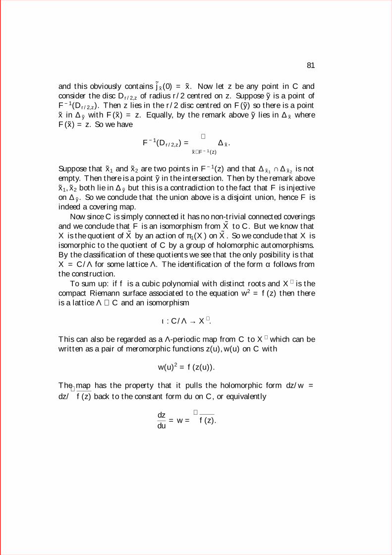
81
and this obviously contains jx(0) = x. Now let z be any point in C andconsider the disc Dr/2,z of radius r/2 centred on z. Suppose y is a point ofF−1(Dr/2,z). Then z lies in the r/2 disc centred on F (y) so there is a pointx in ∆y with F (x) = z. Equally, by the remark above y lies in ∆x whereF (x) = z. So we have
F−1(Dr/2,z) =⋃
x∈F−1(z)
∆x.
Suppose that x1 and x2 are two points in F−1(z) and that ∆x1 ∩∆x2 is notempty. Then there is a point y in the intersection. Then by the remark abovex1, x2 both lie in ∆y but this is a contradiction to the fact that F is injectiveon ∆y. So we conclude that the union above is a disjoint union, hence F isindeed a covering map.
Now since C is simply connected it has no non-trivial connected coveringsand we conclude that F is an isomorphism from X to C. But we know thatX is the quotient of X by an action of π1(X) on X. So we conclude that X isisomorphic to the quotient of C by a group of holomorphic automorphisms.By the classification of these quotients we see that the only posibility is thatX = C/Λ for some lattice Λ. The identification of the form α follows fromthe construction.
To sum up: if f is a cubic polynomial with distinct roots and X∗ is thecompact Riemann surface associated to the equation w2 = f(z) then thereis a lattice Λ ⊂ C and an isomorphism
ι : C/Λ→ X∗.
This can also be regarded as a Λ-periodic map from C to X∗ which can bewritten as a pair of meromorphic functions z(u), w(u) on C with
w(u)2 = f(z(u)).
The map has the property that it pulls the holomorphic form dz/w =
dz/√f(z) back to the constant form du on C, or equivalently
dz
du= w =
√f(z).
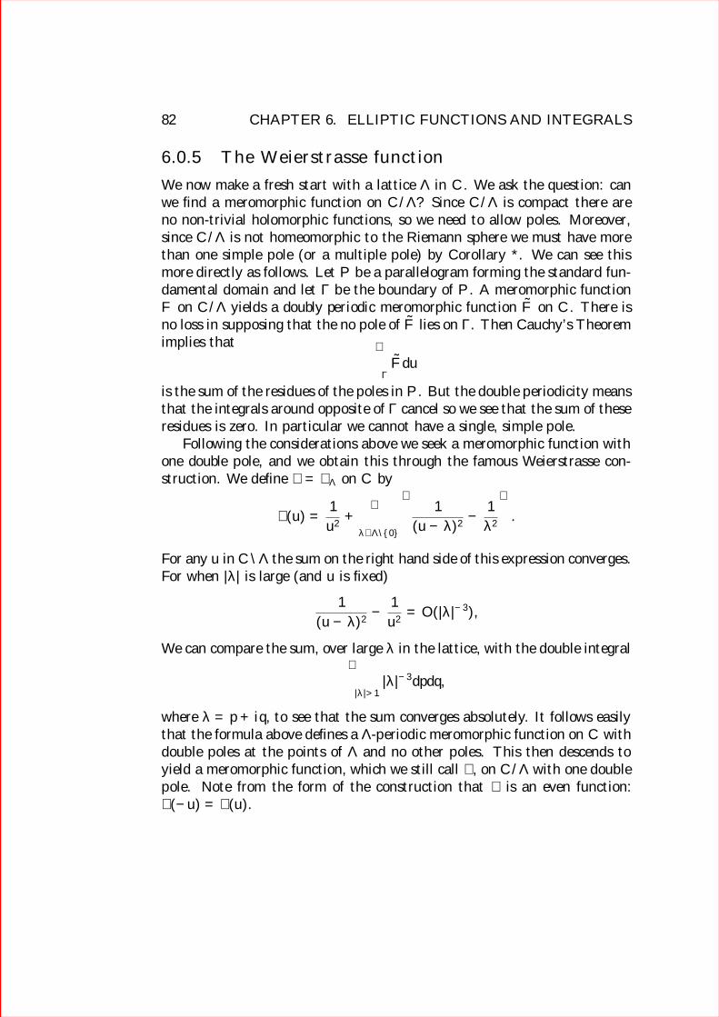
82 CHAPTER 6. ELLIPTIC FUNCTIONS AND INTEGRALS
6.0.5 The Weierstrasse function
We now make a fresh start with a lattice Λ in C. We ask the question: canwe find a meromorphic function on C/Λ? Since C/Λ is compact there areno non-trivial holomorphic functions, so we need to allow poles. Moreover,since C/Λ is not homeomorphic to the Riemann sphere we must have morethan one simple pole (or a multiple pole) by Corollary *. We can see thismore directly as follows. Let P be a parallelogram forming the standard fun-damental domain and let Γ be the boundary of P . A meromorphic functionF on C/Λ yields a doubly periodic meromorphic function F on C. There isno loss in supposing that the no pole of F lies on Γ. Then Cauchy’s Theoremimplies that ∫
ΓF du
is the sum of the residues of the poles in P . But the double periodicity meansthat the integrals around opposite of Γ cancel so we see that the sum of theseresidues is zero. In particular we cannot have a single, simple pole.
Following the considerations above we seek a meromorphic function withone double pole, and we obtain this through the famous Weierstrasse con-struction. We define ℘ = ℘Λ on C by
℘(u) =1
u2+
∑λ∈Λ\0
(1
(u− λ)2− 1
λ2
).
For any u in C\Λ the sum on the right hand side of this expression converges.For when |λ| is large (and u is fixed)
1
(u− λ)2− 1
u2= O(|λ|−3),
We can compare the sum, over large λ in the lattice, with the double integral∫|λ|>1|λ|−3dpdq,
where λ = p+ iq, to see that the sum converges absolutely. It follows easilythat the formula above defines a Λ-periodic meromorphic function on C withdouble poles at the points of Λ and no other poles. This then descends toyield a meromorphic function, which we still call ℘, on C/Λ with one doublepole. Note from the form of the construction that ℘ is an even function:℘(−u) = ℘(u).

83
Now ℘ has a Laurent expansion about 0:
℘(u) =1
u2+ 0 + au2 + bu4 + . . . ,
where the vanishing of the coefficient of u0 follows from the shape of theconstruction. This gives
℘′′(u) =6
u4+ 2a+ . . . ,
so℘′′ − 6℘2 = −10a+ . . . ,
is a holomorphic Λ-periodic function, hence constant. Thus ℘′′ − 6℘2 = 10a.We can rewrite this identity as
d
du
(℘′2)
=d
du
(4℘3 − 20a℘
)so ℘′2 = 4℘3−20a℘+a′, say, with a′ another constant. Adopting conventionalnotation, ℘ satisfies an equation
d℘
du
2
= 4℘3 − g2℘− g3,
for certain constants g2, g3 depending on the lattice.Exercise Show that
g2 = 60∑λ∈Λ′
λ−4
g3 = 160∑λ∈Λ′
λ−6
where Λ′ denotes Λ \ 0.Now this just expresses the fact that C/Λ arises as the Riemann surface
associated to an equation w2 = f(z) for cubic f so our conclusion is that theclasses of Riemann surfaces obtained in these two ways are identical. Re-turning finally to our starting point we see that the solution of the pendulumequation can be written as
θ = cos−1(℘Λ(t+ t0)),
for a suitable lattice Λ.
Exercise. Show that the lattice Λ associated to the pendulum equationis rectangular, generated by 1 and iq for some q > 0, and that for the physicalsolutions the imaginary part of the constant of integration t0 must be q/2.

84 CHAPTER 6. ELLIPTIC FUNCTIONS AND INTEGRALS

Chapter 7
Applications of the Eulercharacteristic
We have seen that the genus of a compact oriented smooth surface S can bedefined as one half the dimension of the de Rham cohomology group H1(S).There are many other possibilities. In particular another way of defining thegenus, in some respects more elementary, uses the Euler characteristic. Thiscan be done via triangulations of the surface. We do not want to take thetime to develop the theory of triangulations in detail but we will describe thisapproach slightly informally here and then develop some applications. Thereader with a suitable background in topology will know how to make the dis-cussion more rigorous and in any case we will be able to derive the corollariesas simple consequences of the more advanced theory (the Riemann-Roch for-mula) later. Howver we give this more elementary discusion now, since we donot want the reader to gain the impression that these essentially topologicalresults depend essentially on the rather deeper analysis in Part III.
7.1 The Euler characteristic and meromor-
phic forms
7.1.1 Topology
Suppose we have a surface, posibly with boundary, which is triangulated inthe manner indicated.
85

86CHAPTER 7. APPLICATIONS OF THE EULER CHARACTERISTIC
Then the Euler characteristic of the triangulation is defined to be
χ = V − E + F
where V,E, F are the number of vertices, edges and faces respectively. Thefirst basic fact is that number is independent of the choice of triangulation,hence defines an integer χ(S) the Euler characteristic of S. It is not hardto check, for example by defining explicit triangulations, that for the modelsurfaces
χ(Σg,r) = 2− 2g − r, χ(Ξh,r) = 2− h− r.We can define the genus of a closed oriented surface by g = 1 − χ(S)
2and of
course the next thing we need to know is that this coincides with our previousdefinition. If we are willing to accept the classification of surfaces of coursethere is no need to have any theory here, since we just need to check forthe model surfaces. But is preferable from many points of view (for example,extensions to higher dimensions) to understand the result independent of theclasification of surfaces. In any case, let us assume it from now on.
Now suppose S is a compact oriented surface and that α is a real 1-formon S. Suppose that the set ∆ ⊂ S where α vanishes is discrete. Given anypoint p of ∆ we choose local co-ordinates centred on p and represent α locallyas
α = α1dx1 + alpha2dx2.
Our hypothesis asserts that for small r the only zero of the vector-valuedfunction (α1, α2) on the closed r-disc about the origin is at the origin itself.Thus the restriction of this function to a circle of radius r gives a map fromthe circle to R2 \ 0 which has an integer winding number. It not hardto check that this is indpendent of teh choice of r and the local co-ordinatesystem. We define the multiplicity mp(α) of the zero p of α to be this windingnumber.
Proposition 15 In the situation above∑p∈∆
mp(α) = −χ(S).

7.1. THE EULER CHARACTERISTIC AND MEROMORPHIC FORMS87
We sometimes call the sum on the left hand side of this formula the “numberof zeros of α(counted with multiplicity)”. Of course there are many differentways of building up this theory. For example if one shows that the sumof zeros (counted with multiplicity) is independent of teh choice of α thenone can use it to define the Euler characteristic, and hence the genus. Torelate this to the count in the definition by triangulations one can consider astandard 1-form on a triangle given by df where f is the function indicatedby the following picture.
If we have a triangulation of S then we can define a 1-form on S whichrestricts to this model on each triangle. There is then one zero for eachvertex, one for each edge and one for each face: the multiplicities are all +1for the first and third case and −1 for the second. So the “count” of zerosgives precisely the count of vertices, edges and faces, with the right signs. Inany case what we will assume known is that Proposition * holds true for anysmooth 1-form α with discrete zero-set and where χ(S) = 2− 2g with g thegenus defined in Chapter *.
7.1.2 Meromorphic forms
Now suppose that X is a compact Riemann surface and that α is a holomor-phic 1-form on X, not identically zero. We associate to this the real 1-formA = α + α In a local co-ordinate z we write α = f(z)dz; the zeros of A arethe zeros of f hence discrete. Moreover the multiplicity of a zero is a positiveinteger, equal to the multiplicity of the zero of f in the usual sense. Hencein this case Proposition * says that the total number of zeros counted withthese positive multiplicities, is 2g − 2. In particular if g = 0 there can beno such α and if g = 1, the situation considered in the previous Chapter, anon-trivial holomorphic form is nowhere vanishing.
We can extend this discussion to meromorphic 1-forms. To do this we fixan area form ω on X. This means that we can define a Hermitian metric onT ∗X ′:
ξ ∧ ξ = |ξ|2ω.

88CHAPTER 7. APPLICATIONS OF THE EULER CHARACTERISTIC
Suppose α is a meromorphic 1-form on X. Choose a real-valued function pon R with p(t) = 1 for small t and p(t) = t−1 for large t. Now define
α = p(|α|2α,
away from the poles of α and α = 0 at the poles of α. Locally, around a poleof α, we have
α =1
|f(z)|2f(z)Rdz = f(z)Rdz
where R is a smooth strictly positive function. Thus tilde α is smooth andits zero set is the union of the zeros and poles of α. It is clear that the zerosof α corresponding to the poles of α have multiplicity equal to minus theorder of the pole. Thus we have
Proposition 16 If α is a nontrivial meromorphic 1-form on a compact Rie-mann surface X then the number of zeros of α minus the number of poles ofα, counted with multiplicity is equal to 2g − 2.
7.2 Applications
7.2.1 The Riemann-Hurwitz formula
Suppose that f : X → Y is a nonconstant holomorphic map between con-nected compact Riemann surfaces. In Chapter 4 we have associated a multi-plicity kx to each point of X, equal to 1 except for a finite set of ramificationpoints. We define the total ramification index to be
Rf =∑x∈X
kx − 1.
So this is really a finite sum. We have also defined the degree d ≥ 1 of themap.The following result, the Riemann Hurwitz formula, is very useful forcalculations
Proposition 17 The genus gXof X and the genus gY of Y are related
2− 2gY = d(2− 2gX)−Rf .
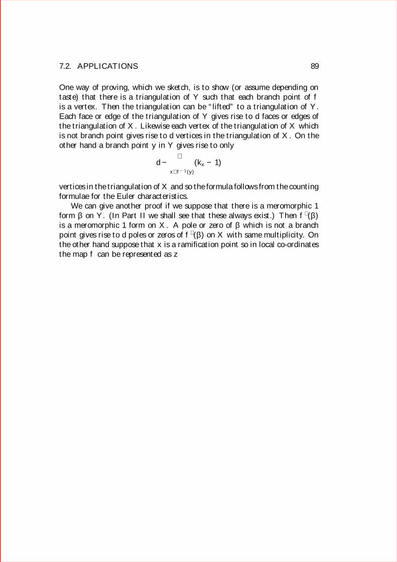
7.2. APPLICATIONS 89
One way of proving, which we sketch, is to show (or assume depending ontaste) that there is a triangulation of Y such that each branch point of fis a vertex. Then the triangulation can be “lifted” to a triangulation of Y .Each face or edge of the triangulation of Y gives rise to d faces or edges ofthe triangulation of X. Likewise each vertex of the triangulation of X whichis not branch point gives rise to d vertices in the triangulation of X. On theother hand a branch point y in Y gives rise to only
d− ∑x∈f−1(y)
(kx − 1)
vertices in the triangulation of X and so the formula follows from the countingformulae for the Euler characteristics.
We can give another proof if we suppose that there is a meromorphic 1form β on Y . (In Part II we shall see that these always exist.) Then f ∗(β)is a meromorphic 1 form on X. A pole or zero of β which is not a branchpoint gives rise to d poles or zeros of f∗(β) on X with same multiplicity. Onthe other hand suppose that x is a ramification point so in local co-ordinatesthe map f can be represented as z 7→ w = zk, where k = kx > 1. If β is thegiven in the w co-ordinate by g(w)dw for some meromorphic g the pull-backf ∗(β) is
kzk−1g(zk)dz.
If g has a zero of order l ∈ Z (where a negative value of l indiactes a polein the obvious way) then zk−1g(zk) has a zero of order kl + k − 1. So thecontribution to the count of zeros/poles of f ∗(β) from the points x in f−1(y)is ∑
x∈f−1(y)
(kxl + kx − 1) = dl +∑
x∈f−1(y)
(kx − 1),
since we know thatd =
∑x∈f−1(y)
(kx − 1).
Then applying * to β and f ∗(β) we obtain the Riemann-Hurwitz formula.
7.2.2 The degree-genus formula
Now suppose that X is a smooth complex curve of degree d in CP2. Recallthat this means that X is defined by a homogeneous polynomial p(Z0, Z1, Z2)and that not all of the partial derivatives ∂p
∂Zivanish at any point of X.

90CHAPTER 7. APPLICATIONS OF THE EULER CHARACTERISTIC
Proposition 18 The genus of X is given by
gX =1
2(d− 1)(d− 2).
For example we have already seen that when d = 1 or 2 the Riemannsurface X is equivalent to the Riemann sphere (genus 0), and when d = 3 toa complex torus C/Λ (genus 1). Notice that this shows that some compactRiemann surfaces cannot be realised as smooth curves in CP2, since not allintegers can be expressed as (d− 1)(d− 2)/2.
There are various ways of obtaining the formula in the Proposition. Wewill establish the result by contructing a meromorphic form on X and count-ing the poles and zeros. Suppose for simplicity that the curve X meets theline at infinity in d distinct points. (It is easy to show that this can be ar-ranged by a suitable linear transformation of the Zi.) Let P (z, w) be thepolynomial in 2 variables defining the corresponding affine curve X0. We fol-low the same construction that we used, in a special case, in Chapter 5. Thusdz, dw represent holomorphic 1-forms on X0 and the identity P (z, w) = 0 onX0 yields
Pzdz + Pwdw = 0.
At points where Pz, Pw are both non-zero we have
dz
Pw= −dw
Pz.
Since, by hypothesis, there are no points on X0 where Pz, Pw both vanishwe obtain a non-vanishing holomorphic 1-form θ on X0 equal to dz/Pw or−dw/Pz at the points where these are defined. We have to check that θ isa meromorphic 1-form on X, i.e. that it has at worst poles at the d pointsof intersection with the line at infinity, and then count the zeros or poles atthese points.
7.2.3 Real structures and Harnack’s bound
In Chapter 2 we discussed nonorientable surfaces, indeed this was the mostinteresting case from the point of view of the classification theorem, but sincethen they have dropped out of the picture, mainly because any Riemannsurface is oriented. However non-orientable surfaces do arise naturally incertain questions, as we will now illustrate.

7.2. APPLICATIONS 91
In Chapter 3 we have defined the notion of holomorphic maps betweenRiemann surfaces. One can just as well define antiholomorphic maps: givenin local complex coordinates by antiholomorphic functions (a function f onan open set in C is antiholomorphic if f is holomorphic. The composite ofantiholomorphic maps is holomorphic and the composite of a holomorphicmap and an antiholomorphic map is antiholomorphic. We say that a realstructure on a Riemann surface X is an antiholomrphic map σ : X → X withσσ equal to the identity. The real points XR of such a pair (X, σ) are definedto be the fixed points of σ. For example the maps σ0, σ1 : C \ 0 → C \ 0given by
σ0(z) = z , σ1(z) = −1/z,
are two different real structures on C \ 0. The real points being the realaxis in one case and the empty set in the other. Each of these extends toa real structure on the Riemann sphere and S2
R is a copy of a circle in onecase and empty in the other.
Proposition 19 Let (X, σ) be a Riemann surface with a real structure andx be a point of XR ⊂ X. There is a local holomorphic co-ordinate z aroundx in which σ is given by the map z 7→ z.
The proof is an exercise for the reader.If (X, σ) is a surface with a real structure we can form the quotient space
X/σ. Using the proposition above it is not hard to show
Proposition 20 The space X/σ is a surface with boundary, where the bound-ary of X/σ can be identified with XR.
(More precisely we should say that X/σ can be endowed with structure ofa surface with boundary.) The quotient X/σ may be orientable or non-orientable and the boundary may or may not be empty. For example withthe two real structures σ0, σ1 on S2 above S2/σ0 is a disc and S2/σ1 is thereal projective plane RP2.
Now suppose that X is a compact connected Riemann surface with a realstructure σ. Then X/σ is a compact connected surface with boundary. Wehave
Proposition 21 The Euler characteristics of X and X/σ satisfy
χ(X) = 2χ(X/σ).

92CHAPTER 7. APPLICATIONS OF THE EULER CHARACTERISTIC
Just as with the Riemann-Hurwitz formula various proofs are possible.In terms of triangulations, if we choose a triangulation of X/σ we can lift toa triangulation of X. Then to each face of X/σ correspond two faces of Xand likewise to each vertex and edge which do not lie in the boundary. Onthe other hand each edge and vertex in the boundary of X/σ correspond tojust one edge or vertex in X. But each component of the boundary of X/σis a circle, so clearly the numbers of edges and vertices in the boundary areequal. Then the result follows from simple counting.
Now for any surface with boundary Y with r boundary components wehave
χ(Y ) ≤ 2− r,with equality in the case when Y is a sphere with r discs removed. If weaccept the classification of surfaces we can read this assertion off from that:an independent proof is also possible of course. In any case we obtain theconclusion
Proposition 22 Let X be a compact connected Riemann surface of genusg. If σ is a real structure on X then the number of components of XR is atmost g + 1.
This follows immediately from the discussion above, since if r is the numberof components of XR we have
1− g =1
2χ(X) = χ(X/σ) ≤ 2− r
since r is also the number of boundary components of X/σ.Equality holds in the case when σ is the reflection map acting on the
standard picture of a surface of genus g, and the quotient is a sphere withg + 1 discs removed.
.To give a concrete application of this, suppose that P is a polynomial in
two variables with real co-efficients. Then, regarded as a complex polynomial,

7.2. APPLICATIONS 93
P defines an affine curve in C2 and a projective curve X in CP2. Suppose forsimplicity that these are smooth. Complex conjugation of the co-ordinatesinduces a real structure on X and the set XR just corresponds to the pointsof the corresponding real projective curve in RP2. So we have Harnack’sbound
Proposition 23 Let p be a homogeneous polynomial with real co-efficientsand degree d in three variables with the property that the corresponding com-plex projective curve is smooth. Let Γ ⊂ RP2 be the real projective curve de-fined by p. Then the number of components of Γ is at most 1
2(d−1)(d−2)+1.
(It is not hard to remove the hypothesis on the smoothness of the complexprojective curve.)
7.2.4 Modular curves
In Chapter 3 we introduced the modular curves Xa, the quotients of theupper half plane by the group Γa. From the definition it was not clear howto say much about these. We will now see how to understand the topologyof these Riemann surfaces, for simplicity we restrict to the case when a isprime.
Proposition 24 If p is a prime number, not equal to 2, then there is acompact Riemann surface Xp of genus
g = 1 +
((p− 6)(p2 − 1)
24
)
with a subset ∆ ⊂ Xa containing (p2−1)/2 points, such that Xp is equivalentto the complement Xp \∆.

94CHAPTER 7. APPLICATIONS OF THE EULER CHARACTERISTIC

Part III
Deeper Theory
95


Chapter 8
Meromorphic functions and theMain Theorem for compactRiemann surfaces
This Section does not contain much technical content but is crucial in ex-plaining our strategy for proving the fundamental structural results aboutRiemann surfaces. For motivation, we can review the discussion of surfacesof genus 1 in the previous section. Suppose we have a general compact Rie-mann surface X of genus 1. We can show that X is equivalent to one of thefamily of surfaces studied in the previous Chapter if we can show either:
• That there is a meromorphic function with a double pole (or two singlepoles) on X. This then represents X as a two sheeted cover of theRiemann sphere with four branch points.
or
• That there is a nowhere-vanishing holomorphic 1-form on X. Then wecan apply Theorem * to see that X is a complex torus C/Λ.
This motivates our task, which is to get a good understanding of the ex-istence of meromorphic functions, holomorphic 1-forms and the relationshipbetween these for general compact Riemann surfaces.
Recall that on any Riemann surface X we have the “square” of differentialoperators *. We define complex vector spaces
H0,0X = Ker∂ : Ω0 → Ω0,1.
97

98CHAPTER 8. MEROMORPHIC FUNCTIONS AND THE MAIN THEOREM FOR COMPACT RIEMANN SURFACES
H1,0X = Ker∂ : Ω1,0 → Ω2.
H0,1X = Coker∂ : Ω0 → Ω0,1.
H1,1X = Coker∂ : Ω1,0 → Ω2.
Thus H0,0X , H1,0
X are the spaces of holomorphic functions and holomorphic 1-forms respectively. The significance of the other groups is not so clear. Whatwe want to do now is to explain how H0,1
X arises naturally when one attemptsto construct meromorphic functions.
Let p be a point in X. We ask the question: is there a meromorphicfunction on X with a simple pole at p and no other poles? Let z be a localco-ordinate centred on p. Thus 1
zcan be regarded as a meromorphic function
on some open neighbourhood U of p. We introduce a cut-off function β; asmooth function supported in U and equal to 1 near p. Then β 1
zcan be
thought of as a function on X \ p, extending by zero outside U . Findinga meromorphic function with a pole at p is equivalent to finding a smoothfunction g on X such that g + β 1
zis holomorphic on X \ p. Now
A = ∂(β1
z) = (∂β)
1
z
has compact support in X \ p since β equals 1 near p. So we can regardA as a (0, 1) form on X, extending by zero over p. Thus our problem isequivalent to solving the equation
∂g = −Afor the given element A of Ω0,1
X and the unknown g ∈ Ω0X . By definition, a
solution exists if and only if the class [A] in the quotient H0,1X = Coker∂ =
Ω0,1/Im∂ is zero. In particular, a solution will exist if H0,1X = 0. Even if a
solution does not exist, the class [A] is, up to multiplication by a non-zeroscalar, a well-defined element of H0,1
X associated to the point p in X. Forif φ is any smooth function on X \ p which restricts to a meromorphicfunction with a pole at p on some neighbourhood of p then for a suitablechoice of λ ∈ C the difference φ − λβ 1
zextends to a smooth function on X
(holomorphic near p) so
[∂φ] = λ[A] ∈ H0,1X .
Now suppose that we have d distinct points p1, . . . pd in X. We ask ifwe can find a meromorphic, but not holomorphic, function on X with poles

8.1. CONSEQUENCES OF THE MAIN THEOREM 99
at some, or all, of the pi and no other poles. We follow through the sameprocedure as before, choosing local co-ordinates around the pi to get (0, 1)forms Ai, which we can take to be supported in small disjoint annuli aroundthe pi if we like. The same argument as before shows that we can find thedesired meromorphic function if there are scalars λi, not all zero, such that
λ1[A1] + . . .+ λd[Ad] = 0 ∈ H0,1X .
Given such a linear relation we get a meromorphic function with poles at thepoints pj for which λj 6= 0. In particular we have
Proposition 25 Suppose H0,1X has finite dimension h. Then given any h+1
points p1, . . . , ph on X there is a non-holomorphic meromorphic function onX with simple poles at some subset of the p1, . . . , ph.
This is just because there must be a non-trivial linear relation between anyh+ 1 elements of H0,1
X .The discussion aboves shows how we can cast our problem in terms of the
spaces H0,1X but it does not by itself get as very far. To go further we need
some much deeper input and we will formulate this in terms of the following“Main Theorem for compact Riemann surfaces” (not standard terminology):
Theorem 4 Let X be a compact connected Riemann surface and let ρ be a2-form on X. there is a solution f to the equation ∆f = ρ if and only theintegral of ρ over X is zero.
We will give a proof of this Theorem in the next section, but let us see someconsequences first.
8.1 Consequences of the main theorem
The relation between the “Dolbeault cohomology” H i,j and the de Rhamcohomology H i can be summarised as follows We have the following naturalmaps
• A map σ : H1,0 → H0,1 induced by α 7→ α.
• A bilinear map
B : H1,0 ×H0,1 → C,

100CHAPTER 8. MEROMORPHIC FUNCTIONS AND THE MAIN THEOREM FOR COMPACT RIEMANN SURFACES
defined by
B(α, [θ]) =∫Xα ∧ θ.
(This is well defined since changing the representative θ to θ + ∂fchanges the integral by∫
Xα ∧ ∂f = −
∫X∂(fα),
which vanishes by Stokes’ Theorem.)
• A map i : H1,0 → H1 defined by mapping a holomorphic (hence closed)1-form to its cohomology class.
• A map ν : H1,1 → H2 defined to be the natural map indced from theinclusion Im : ∂ : Ω0,1 → Ω2 ⊂ Im : d : Ω1 → Ω2,
Theorem 5 Let X be a compact connected Riemann surface.
1. The map σ induces an isomorphism from H1,0 to H0,1.
2. The pairing B induces an isomorphism H0,1 ∼= (H1,0)∗.
3. The map H1,0 ⊕H0,1 → H1 defined by
(α, θ) 7→ i(α) + i(σ−1(θ))
is an isomorphism.
4. The map ν : H1,1 → H2 is an isomorphism.
The proofs are entirely straightforward applications of the main theorem.To show that σ is surjective we start with any class [θ] in H0,1. We wantto find a representative θ′ = θ + ∂f such that ∂θ = 0. For this means thatα = overlineθ′ is a holomorphic 1-form and [θ] = −σ(α). Thus we want tosolve the equation
∂∂f = −∂θ.Since ∂∂ = 1
2i∆ the main theorem tells us that we can solve this equation
provided the integral of ∂θ vanishes, but this is so by Stokes’ theorem.Now the composite of the map i with the bilinear pairing B is up to factor
the Hermitian form〈α, β〉 =
∫Xα ∧ alpha

8.1. CONSEQUENCES OF THE MAIN THEOREM 101
which we know is positive definite. It follows that the map i must be injectiveand in turn that B is a dual pairing. We leave the other parts as an exercisefor the reader.
We see in particular from the Corollary that both H1,0, H0,1 are complexvector spaces of dimension g. Thus the genus, which was initially a topolog-ical invariant appears also as teh crucial numerical invariant of the complexgeometry of a Riemann surface.
We can give some simple consequences of the above.
Corollary 3 Any compact Riemann surface X with H1(X) = 0 is equivalentto the Riemann sphere.
Corollary 4 Any compact Riemann surface with g = 1 is equivalent to atorus C/Λ.
Corollary 5 Let X be a compact riemann surface of genus g and let p1, . . . , pgbe distinct points on X. Then there is a non-constant meromorphic functionon X with poles at some subset of the pi.

102CHAPTER 8. MEROMORPHIC FUNCTIONS AND THE MAIN THEOREM FOR COMPACT RIEMANN SURFACES

Chapter 9
Proof of the Main Theorem
9.1 Discussion and motivation
We will now embark on the proof of our main analytical result, thm:mainthmfor compact Riemann surface. Before getting to work we give some prelim-inary discussion. The Theorem really consists of the three statements, on acompact connected Riemann surface X,
• If there is a solution to the equation ∆φ = ρ then the integral of ρ iszero.
• If there is a solution it is unique up to the addition of a constant.
• Conversely if ρ is a form of integral 0 we can find a solution φ.
The first and second of these three statements are very easy to prove, sothe real content is the third statement. The first statement follows immedi-ately from Stokes’ Theorem, since for any φ,∫
X∆φ = 2i
∫X∂∂φ = 2i
∫Xd(∂φ) = 0.
The second statement is equivalent to the assertion that the only har-monic functions—solutions of the equation ∆f = 0—are the constants. Onecan see this in two ways: either by the maximum principle for harmonic func-tions or by considering the Dirichlet integral. For the first one considers apoint in X where f is maximal, which exists by the compactness assumption,and applies the maximum principle at that point. For the second one writes∫
X|df |2 =
∫Xf∆f = 0,
103

104 CHAPTER 9. PROOF OF THE MAIN THEOREM
when ∆f = 0. Thus df vanishes everywhere on X and f is a constant. Thesetwo proofs of the uniqueness are both very simple but the two approachesare manifestations of two different approaches—via the maximum principle orDirichlet integral— which can be taken to the whole theory. To illustrate thisconsider a problem which is closely related to that considered our Theorem,the solution of the Dirichlet boundary value problem. Here we consider abounded domain Ω ⊂ C with smooth boundary ∂Ω and a given function gon the boundary. The problem is to solve the equation ∆φ = 0 in Ω withthe boundary condition that φ has a continuous extension to Ω, equal to gon the boundary. Supposing that a solution φ exists one can show that it ischaracterised by two different extremal properties.
1. For each x in Ω,
φ(x) = minψ(x) : ψ|∂Ω = g,∆ψ ≥ 0.
2. The function φ minimises∫
Ω |∇ψ|2 over all functions ψ on Ω withψ|∂Ω = g.
Conversely, one can prove the existence of a solution φ by showing that suchextremal functions exist. Both of these approaches have their own merits andgeneralise in different ways. The line we will take in the proof of the MainTheorem, and the further results in the next Chapter, will follow the Dirichletintegral approach, closest to the heuristic arguments originally employed byRiemann.
The equation ∆φ = ρ is, in local co-ordinates, the Poisson equationwhich may be familiar from potential theory in Rn. In this vein, one canobtain some physical intuition into why the main theorem should be true,as follows. In this discussion we will anticipate a result proved in Chapter13, that an oriented surface in R3 is naturally a Riemann surface. Supposethe Riemann surface X arises this way. We get a standard area form onX, so we can identify the 2-forms and the functions. Think of this surfacein R3 as being made of a thin metal sheet and the function φ as being thetemperature distribution over the sheet. The function ρ represents someexternally imposed source or removal of heat, varying over the surface. Thenthe Poisson equation ∆φ = ρ is the equation for a steady-state temperaturedistribution, and the content of our Theorem is that if the integral of ρ iszero—so there is no overall gain or loss of heat—then such a temperature

9.1. DISCUSSION AND MOTIVATION 105
distribution exists. One can also think about this in terms of the time-dependent heat equation
∂φ
∂t= ρ−∆φ.
Here φ is now a function on X×[0,∞) while we still suppose that ρ is constantin time. One can prove analytically, in line with ones physical intuition, thatif the integral of ρ is zero then for any initial temperature distribution thisheat equation has a solution which converges as t→∞ to a solution of . thePoisson equation.
One case in which the Theorem can be proved easily is that of a torus.Suppose for example that X is the quotient of C by the “square” lattice2πZ ⊕ 2πiZ. We take standard real angular co-ordinates θ1, θ2 on X andidentify functions with 2-forms in the obvious way. Any smooth function onX can be written as a c=double Fourier series
f =∑n,m
fnmeinθ1+imθ2 .
The Laplacian of such a function is
∆f =∑
(n2 +m2)fn,meinθ1+imθ2 ,
and the integral of f , with respect to the standard area form, is 4π2f00. Thusif ρ has integral zero we can write down the solution to the Poisso equationin the form
φ =∑
(m,n) 6=(0,0)
1
m2 + n2ρmne
imθ1+nθ2 ,
where ρmn are the Fourier coefficients ofρ.As a final remark, it is worth pointing out that our Theorem fits into a
wider setting of elliptic differential operators on compact manifolds. We donot pause to explain what is meant by an elliptic operator: suffice it to saythat this is a class of linear differential operators which includes the Laplaceoperator ∆ as a particular case. If L is any linear differential operator overa compact manifold, and if we choose appropriate volume forms etc., thereis a formal adjoint operator L∗, characterised by the fact that for any f, g
〈Lf, g〉 = 〈f,L∗g〉,where 〈 , 〉 denotes the L2 inner product. Then the main result is that if Lis elliptic one can solve the equation
Lφ = ρ

106 CHAPTER 9. PROOF OF THE MAIN THEOREM
if and only if ρ is orthogonal, in the L2 sense, to the kernel of L∗. In theRiemann surface situation of Theorem *, if we choose a an area form on thesurface to identify functions and 2-forms the formal adjoint of the Laplacianis the same operator, ∆∗ = ∆, so the kernel of ∆∗ consists of the constantfunctions and the condition that ρ be orthogonal to this kernel is just thatthe integral of ρ is zero.
9.2 The Riesz representation theorem
We will now begin the proof. As we have said above, our approach will hingeon the Dirichlet integral and an efficient way to build this in to the argumentuses the language of Hilbert spaces. Recall that we have defined the Dirichletnorm and inner product on functions on X. The norm and inner productare unchanged if we modify our functions by the additions of constants. Welet C∞(X)/R be the vector space obtained by dividing out by the constantfunctions, so the norm and inner product descend to this quotient. Then wehave
Proposition 26 The Dirichlet norm and inner product make C∞(X)/Rinto a pre-Hilbert space.
(Our notation will sometimes blur the distinction between a function onX and the equivalence class in C∞(X)/R which it represents. Note that ifwe fix a metric, i.e. area form, on X we can identify C∞(X)/R with thespace of functions on X of integral zero.)
Now suppose that ρ is a 2-form on X. For any functions φ, ψ on X wehave∫Xψ(ρ−∆φ) =
∫Xψρ−
∫Xψ∆φ =
∫Xψρ−
∫X∇φ.∇ψ =
∫Xψρ− 〈φ, ψ〉D.
By a simple, standard, argument the equation ∆φ = ρ is equivalent to thecondition that for all functions ψ we have∫
Xψ(ρ−∆φ) = 0.
Thus the content of

9.2. THE RIESZ REPRESENTATION THEOREM 107
Theorem 6 :mainthm can be reformulated as the assertion that, when∫X ρ =
0 there is a function φ such that∫Xψρ = 〈ψ, φ〉D,
for all ψ ∈ C∞(X). To write this more compactly, define
ρ(ψ) =∫Xρψ.
Then, if the integral of ρ is zero, this induces a linear map
ρ : C∞(X)/R→ R,
and our problem is to find a φ such that
ρ(ψ) = 〈ψ, φ〉Dfor all ψ.
In this formulation, our problem falls into the class covered by the well-known Riesz representation theorem from Hilbert space theory.
Theorem 7 Let H be a real Hilbert space and σ : H → R be abounded linearmap (so there is a constant C such that |σ(x)| ≤ C‖x‖ for all x ∈ H). Thenthere is a z ∈ H such that
σ(x) = 〈z, x〉,for all x in H.
For a proof see almost any elementary functional analysis text bookWith all this background in place, we can see that the proof of * divides
into two parts. First, we want to put ourself into the position where wecan apply the Riesz represention theorem and for this we need a Hilbertspace. Thus we let H be the abstract completion of our pre-Hilbert spaceC∞(X)/R, under the Dirichlet norm ‖ ‖D. A point of H is an equivalenceclass of Cauchy sequences (ψi) in C∞(X)/R under the equivalence relation(ψi) ∼ (ψ′i) if ‖ψi − ψ′i‖D → 0. The crucial thing we need now is
Theorem 8 The functional ρ : C∞(X)/R→ R is bounded: there is a con-stant C such that |ρ(ψ)| ≤ C‖ψ‖D for all ψ in C∞(X)/R.

108 CHAPTER 9. PROOF OF THE MAIN THEOREM
Assuming this for the moment, it follows that ρ extends to a boundedlinear map from H to R (which we still denote by ρ. (The proof is just toobserve that for any Cauchy sequence (ψi) in C∞(X)/R the sequence ρ(φi)is Cauchy in R so we can define the extension of ρ by taking the limit.) Sowe can apply the Riesz representation theorem and we conclude that thereis a φ in the completion H with ρ(ψ) = 〈φ, ψ〉D for all ψ. An object of thistype is called a weak solution to our problem and the other part of the proofof Theorem * is to establish
Theorem 9 If ρ is a smooth 2-form on X of integral zero then a weak so-lution φ in H of * is smooth, i.e. lies in the subset C∞(X)/R of H.
9.3 The heart of the proof
The foundation of our proof of Theorem * will be a result from calculus oftwo real variables. Suppose Ω is a bounded, convex, open set in R2. (Forour applications it suffices to consder the case of a circular disc). Let A bethe area of Ω and d be its diameter.
Theorem 10 Let ψ be a smooth function on an open set containing theclosure Ω and let ψ denote the average
ψ =1
A
∫Ωψdµ,
where dµ is the standard Lebesgue measure on R2. Then for x ∈ Ω we have
|ψ(x)− ψ| ≤ d2
2A
∫Ω
1
|x− y| |∇ψ(y)|dµy.
(Here the notation is supposed to indicate that the variable of integration onthe right hand side is y ∈ Ω.)
To prove this there is no loss in supposing that the point x is the originin R2 (applying a translation in R2) and that ψ(0) is zero (changing ψ byaddition of a constant). We work in standard polar co-ordinates (r, θ) on theplane. Thus we can write
ψ =1
A
∫ 2π
0
∫ R(θ)
0ψ(r, θ)rdrdθ,

9.3. THE HEART OF THE PROOF 109
where R(θ) is the length of the portion of the ray at angle θ lying in Ω.(Here we use the fact that Ω is convex.) Now if we introduce another radialvariable ρ we can write, for each (r, θ)
ψ(r, θ) =∫ r
0
∂ψ
∂ρdρ,
using the fact that ψ vanishes at the origin. So now we have
ψ =1
A
∫ 2π
0
∫ R(θ)
0
∫ r
ρ=0ρ∂ψ
∂ρr∂ψ
∂ρdρdrdθ.
We interchange the order of the r and ρ integrals, so
ψ =1
A
∫ 2π
0
∫ R(θ)
ρ=0
(∫ R(θ)
r=ρrdr
)∂ψ
∂ρdrdθ.
The innermost integral is
∫ R(θ)
r=ρrdr =
1
2(R(θ)2 − r2)
which is positive and no larger than R(θ)2
2, while, by definition, R(θ) ≤ d.
Thus
|ψ| ≤ d2
2A
∫ 2π
0
∫ R(theta)
0
1
ρ|∂ψ∂ρ|ρdρdθ.
The modulus of the radial derivative ∂ψ∂ρ
is at most that of the full derivative∇ψ, so switching back to a co- ordinate free notation we have
|ψ| ≤ d2
2A
∫Ω
1
|y| |∇ψy|dµy,
as required.
Corollary 6 Under the hypotheses above
∫Ω|ψ(x)− ψ|2dµx ≤ d2π
2A
∫Ω|∇ψ|2dµ.

110 CHAPTER 9. PROOF OF THE MAIN THEOREM
To prove this, and for later use, we recall the notion of the convolution offunctions on R2. The convolution of functions f, g is defined by
(f ∗ g)(x) =∫
R2f(y)g(x− y)dµy,
The operation * is commutative and associative and if ‖ ‖T is any translation-invariant norm on functions on R2 we have
‖f ∗ g|T ≤ ‖f‖L1‖g‖T ,where ‖f‖L1 is the usual L1 norm
‖f‖L1 =∫R2|f |dµ.
In particular this holds when ‖ ‖T is the L2 norm
‖g‖2L2 =
∫R2|g|2dµ.
(Strictly we should specify what class of functions we are considering in thedefinition of the convolution, but this will be clear in the different contextsas they arise.)
To prove the corollary, we define
K(x) =d2
2A
1
|x| for |x| < d,
and K(x) = 0 if |x| ≥ d. This has a singularity at the origin but is neverthe-less an integrable function and
‖K‖L1 = 2πd2
2A
∫ d
0dr =
d3π
A.
Define a function g on R2 by
g(y) = |∇ψ|2(y),
if y ∈ Ω and g(y) = 0 if y /∈ Ω. Then K ∗ g is a positive function on R2 andTheorem * asserts that for all x ∈ Ω,
|ψ(x)− ψ| ≤ |(K ∗ g)(x).

9.3. THE HEART OF THE PROOF 111
It follows that∫Ω|ψ(x)− ψ|2dµx ≤ ‖K ∗ g‖2
L2 ≤ ‖K‖2L1‖g‖2
L2 ≤(d3π
A
)2
‖∇ψ‖2L2 ,
as asserted.We can now prove *. We begin with the case when ρ is supported in
a single coordinate chart in our Riemann surface, which we identify with abounded convex set Ω in C = R2. Working in this local coordinate systemwe use the Lebesgue area form to identify functions and 2-forms, so ρ can beregarded as a function of integral zero supported on Ω. Likewise, a functionψ on X can be regarded as defining a function, which we also call ψ, on aneighbourhood of Ω in C and we can write
ρ(ψ) =∫
Ωρψdµ.
Now since the integral of ρ is zero we also have
ρ(ψ) =∫
Ωρ(ψ − ψ)dµ,
and by the Cauchy-Schwartz inequality
|∫
Ωρ(ψ − ψ)dµ| ≤ ‖ρ‖L2(Ω)‖ψ − ψ‖L2(Ω).
Using * we then deduce that
|ρ(ψ)| ≤ C‖∇ψ‖L2(Ω),
where C = d3πA‖ρ‖L2(Ω). Finally
‖∇ψ‖L2(Ω) ≤ ‖∇ψ‖L2(X) = ‖ψ‖Dwhich completes the proof of * in this case.
To treat a general 2-form ρ on X, of integral zero, we recall from * thatintegration over X defines an isomorphism from H2(X) to R, so we canwrite ρ = dθ for some 1-form θ on X. We fix a cover of X by a finite numberof coordinate charts Uα ⊂ X of the kind considered above, and choose apartition of unity χα subordinate to this cover. Put ρα = d(χαθ). Then eachρα is supported in the corresponding coordinate chart Uα and∫
Xρα =
∫Xd(chiαθ) = 0

112 CHAPTER 9. PROOF OF THE MAIN THEOREM
On the other hand
ρ = dθ = d((∑
χα)θ) =∑
ρα.
Our previous argument shows that each of the linear maps ρα is boundedand so ρ =
∑ρα is also (as a finite sum of bounded linear maps).
9.4 Weyl’s Lemma
Suppose that φ is an element of H which is a weak solution to our problemin the sense explained above. That is, we have a sequence of functions φi onX which is Cauchy with respect the Dirichlet norm and, for any ψ
〈φi, ψ〉 → ρ(ψ),
as i tends to infinity. We want to see first that we can identify the abstractobject φ with a function (up to a constant) on X, where initially this functionwill just be locally in L2 (i.e. represented by an L2 function, in the ordinarysense, in any local co-ordinate chart). To do this we consider first any fixedco-ordinate chart, identified with Ω ⊂ C, as above. We can suppose, afterchanging the φi by the addition of suitable constants, that the integrals ofthe φi over Ω vanish and then, by cor:poinc, we have
‖φi − φj‖L2(Ω) ≤ C‖φi − φj‖D.Hence φi gives a Cauchy sequence in L2(Ω) which converges to an L2 limit bythe completeness of L2. We claim now that this same sequence φi convergeslocaly in L2 over all of X. We will give the argument in a form which willwork equally well in the generalisation considered in the next Chapter. LetA be the set of points x in X with the property that there is a co-ordinatechart around x in which φi converges to φ in L2. Then A is non-empty bythe preceding discussion and A is open in X from the nature of its definition.Since X is connected, the complement of A is not open, so either A = X orthere is a point y which is in the closure of A but not in A. But in the lattercase we could find a coordinate neighbourhood Ω′ about y and a sequence ofreal numbers c′i such that φi − ’i converges in L2 over Ω′. But now there isa point x in A ∩ Ω′ and on a small neighbourhood of x both φi and φi − c′iconverge in L2. This means that c′i tends to 0 as i→∞, so in fact y is in Aafter all, a contradiction.

9.4. WEYL’S LEMMA 113
To sum up we now have a function φ on X which is locally in L2 andwhich is a weak solution to the equation ∆φ = ρ. We need to show that φis smooth. Since smoothness is a local property we can fix attention on asingle co-ordinate chart. What we need is a version of “Weyl’s lemma”
Proposition 27 Let Ω be a bounded open set in C and ρ be a smooth 2-formon Ω. Suppose is an L2 function on Ω with the property that for any smoothfunction χ of compact support in Ω∫
Ω∆χφ =
∫Ωχρ.
Then φ is smooth and satisfies the equation ∆φ = ρ.
The proof will involve a number of steps. The first step is to reduce to thecase when ρ is zero. Since smoothness is a local property it suffices to provethat φ is smooth over any given interior set Ω′, where we suppose that the εneighbourhood of Ω′ is contained in Ω. Then we can choose a ρ′ equal to ρ ona neighboorhoos of the closure of Ω′ and of compact support in Ω. Supposewe can find some smooth solution φ′ of the equation ∆φ′ = ρ′ over Ω. Thenψ = φ− φ′ will be a weak solution of the equation ∆ψ = 0 on Ω′. If we canprove that ψ is smooth then so will φ be.
To find the smooth solution ψ′ we use the “Newton potential” in twodimensions:
K(x) =1
2πlog |x|.
Of course this is not defined at x = 0 but K is well-defined as a locallyintegrable function on C. For any smooth function f of compact support inC the convolution
K ∗ f(x) =∫K(y)f(x− y)dµy,
is defined and K ∗ f is smooth.
Lemma 14 • If σ has compact support in C then K ∗ (∆σ) = σ.
• If f has compact support then ∆(K ∗ f) = f .
This Lemma essentially expresses the stadard fact that convolution with Kfurnishes an inverse to the Laplace operator. To prove the first assertion wemay, by translation invariance, calculate at the point x = 0. Then
(K ∗∆σ)(0) =∫ 1
2πlog(|y vert)(∆σ)ydµy.

114 CHAPTER 9. PROOF OF THE MAIN THEOREM
Now ∆ log |y vert vanishes on C \ 0. We write the integral as the limitas δ tends to zero of the integral over the set where |y| ≥ δ.We then useGreen’s identity to write this as a boundary integral and then take the limitas δ tends to zero. The argument is rather stabdard so we do not give moredetails.
For the second part we write
(K ∗ f)(x) =∫K(y)f(x− y)dµy.
When we take the Laplacian with respect to x there is no problem in movingthe differential operator inside the integral, since f is smooth and x does notappear inside the argument of K. Thus
∆(K ∗ f) =∫K(y)∆xf(x− y)dµy,
where the notation means that we take the Laplcian with respect to x. Butthis is just the same as K ∗∆f , which is equal to f by the first part.
We have now reduced to the case when ρ = 0 so, changing notation, letus suppose that φ is a weak solution of ∆φ = 0 on Ω and seek to provethat φ is smooth on the interior domain Ω′, with the ε-neighbourhood ofΩ′ contained in Ω. The argument now exploits the mean value propertyof smooth harmonic functions. This says that if ψ is a smooth harmonicfunction on a neighbourhood of a closed disc then the value of ψ at thecentre of the disc is equal to the average value on the circle boundary. Fixa smooth function β on R with β(r) constant for small r and vanishing forr ≥ ε and such that
2π∫ ∞
0rβ(r)dr = 1.
Now let B be the function B(z) = β(|z|) on C. Then B is smooth and hasintegral 1 over C (with respect to ordinary Lebesgue measure). Suppose firstthat ψ is a smooth harmonic function on a neighbourhood of the closed ε-disccentred at the origin. Then we have∫
CB(−z)ψ(z)dµz =
∫ ∞0
∫ 2π
0rβ(r)ψ(r, θ)dθdr = 2πψ(0)
∫ ∞0
rβ(r)dr = 1
where we have switched to polar coordinates and used the mean value prop-erty ∫ 2π
0ψ(r, θ)dθ = ψ(0).

9.4. WEYL’S LEMMA 115
Now the integral above is just that defining the convolution B ∗ ψ at 0. Bytranslation invariance we obtain the following
Proposition 28 Let ψ be a smooth function on C and suppose that ∆ψ issupported in a compact set J ⊂ C. Then B ∗ ψ − ψ vanishes outside theε-neighbourhood of J .
We see in particular from this that if our function φ on Ω is smooth we musthave B ∗φ = φ in Ω′. Conversely, for any L2 function φ the convolution B ∗φis smooth. So proving the smoothness of φ in Ω′ is equivalent to establishingthe identity B ∗ φ = φ in Omega′. To do this we proceed as follows. Itsuffices to show that for any smooth test function χ of compact support inΩ′ we have
〈χ, φ− B ∗ φ〉 = 0,
where we are writing 〈 , 〉 for the usual “inner product”
〈f, g〉 =∫fgdµ.
We use the fact that for any functions f, g, h in a suitable class
〈f, g ∗ h〉 = 〈g ∗ f, h〉.This follows by straightforward re-arrangements of the integrals. We willnot bother to spell out conditions on the functions involved, since it will thevalidity of the identity will be fairly obvious in our applications below.
Put h = K ∗ (χ − B ∗ χ) = K ∗ χ − B ∗K ∗ χ. Now K ∗ χ is a smoothfunction on C and ∆K ∗χ = χ by the Lemma above. Thus ∆K ∗χ vanishesoutside the support of χ, and hence by the Proposition above B∗K ∗χ equalsK ∗χ outside the ε-neighbourhood of the support of χ. Thus h has compactsupport contained in Ω. So we can use h as a test function in the hypothesisthat ∆φ = 0 weakly, i.e. we have
〈∆h, φ〉 = 0.
But ∆h = ∆K ∗ (χ−B ∗ χ) = χ−B ∗ χ by the Lemma above (since χ andB ∗ χ have compact support). So we see that
〈χ− B ∗ χ, φ〉 = 0.
But applying the identity above again this gives
〈χ, φ− B ∗ φ〉 = 0,
as desired.

116 CHAPTER 9. PROOF OF THE MAIN THEOREM

Chapter 10
The Uniformisation Theorem
10.1 Statement
In this chapter we prove
Theorem 11 Let X be a connected, simply connected, non-compact Rie-mann surface. Then X is equivalent to either C or the upper half-planeH.
Corollary 7 Any connected Riemann surface is equivalent to one of
• The Riemann sphere S2;
• C or C/Z = C \ 0 or C/Λ for some lattice Λ;
• A quotient H/Γ where Γ ⊂ PSL(2,R) is a discrete subgroup actingfreely on H,
The Corollary follows because any Riemann surface is a quotient of itsuniversal cover by an action of its fundamental group, and we have seen thatthe only compact simply connected Riemann surface is the Riemann sphere.
Our proof of thm:unif will follow the same general pattern as the one wehave already given to classify compact simply connected Riemann surface,but the noncompactness will require some extra steps. Most of our work goesinto the proof of an analogue of the “Main Theorem”. To state this, recallthat if φ is real-valued function on a non-compact space X and c is a realnumber we say that φ tends to c at infinity in X if for all ε > 0 there is a
117

118 CHAPTER 10. THE UNIFORMISATION THEOREM
compact subset K of X such that |φ(x) − c| < ε if x is not in K. We saythat φ tends to +∞ at infinity in X if for all A ∈ R there is an compact setK ⊂ X such that φ(x) > A if x is not in K (and we say that φ tends to −∞at infinity in X if −φ tends to +∞).
Theorem 12 Let X be a connected, simply-connected, non-compact Rie-mann surface. Then if ρ is a (real) 2-form of compact support on X with∫X ρ = 0 there is a (real valued) function φ on X with ∆φ = ρ and such thatφ tends to 0 at infinity in X.
We now show that thm:potdecay implies thm:unif. Choose a point p ∈ Xand a local complex co-ordinate z around p. Using the same notation as inSection 5, we put
A = ∂(β
z)
where β is a cut-off function, so A is a (0, 1)-form supported in an annulusaround p. We put ρ = ∂A, so ρ is a complex-valued 2-form with integralzero, by Stokes’ Theorem. By the result (applied to the real and imaginaryparts of ρ) we can find a complex-valued function g with ∂∂g = ρ, and withthe real and imaginary parts of g tending to 0 at infinity in X. Now let a bethe real 1-form
a = (A− ∂g) + (A− ∂g).
By construction ∂(A − ∂f) = 0 and this means that da = 0. So, sinceH1(X) = 0, there is a real-valued function ψ with a = dψ. This means thatA = ∂g + ∂ψ. Hence
∂(β
z− (g + ψ)) = 0
on X \ p. Hence f = g+ψ is a meromorphic function on X with a simplepole at p and the imaginary part of f tends to zero at infinity in X, since ψis real. (Strictly the imaginary part of f is not a function on X since f hasa pole, but the meaning should be clear—to be precise we could say that theimaginary part of f tends to 0 at infinity on X \D where D is an open discabout p.)
The meromorphic function f is a holomorphic map from X to the Rie-mann sphere S2 = C∪∞. Let H+, H− denote the (open) upper and lowerhalf-planes in C. Let X± be the preimages f−1(H± in X. So X+ and X−

10.1. STATEMENT 119
are open subsets of X and X+ ∪X− is dense in X, since f is an open map.The restrictions of f gives holomorphic maps
f± : X± → H±.
We claim that f+ and f− are proper maps. For if B is a compact subset ofH+, say, there is an ε > 0 such that =(z) > ε for all z in B. The fact thatthe imaginary part of f tends to zero at infinity implies that f−1(B) is acompact subset of X, but this is the same as f−1
+ (B) ⊂ X+.We know that f yields a local homeomorphism from a neighbourhod of
p in X to a neighbourhood of ∞ in S2. What we see first from this is thatX+, X− are both non-empty. So we have degrees d+, d− ≥ 1 of f+, f−. Weclaim that d+ = d− = 1. To see this we apply the condition that =(f) tendsto zero at infinity to find a compact set K in X such that =(f)(x) < 1 if xis not in K. Suppose the degree of f+ is at least 2. Then for each integern ≥ 1 we can find a pair of points xn, xn ∈ X+ such that f(xn) = f(xn) = inand either xn, xn are distinct or xn = xn and the derivative of f vanishes atxn. The choice of K means that xn, xn lie in this compact set, so we canfind a subsequence n′ such that xn′ and xn′ converge to limits x, x. Sincethe points in, regarded as points of the Riemann sphere, converge to ∞, wemust have f(x) = f(x) = ∞ and since f has just one pole we must havex = x = p. But now we get a contradiction to the fact that f is a localhomeomorphism, with non-vanishing derivative, on a neighbourhhod of p.
So now we know that f maps X± bijectively to H± in C. We claim nextthat f is an injection from X to S2. For if x1, x2 are distinct points of Xwith f(x1) = f(x2) = Z ∈ S2 we can find disjoint open discs D1, D2 aboutx1, x2 and a neighbourhood N of Z ∈ S2 such f(D1), f(D2) each contain N .Now pick a point Z ′ in N ∩ H+. There are distinct points x′1, x
′2 in D1, D2
which map to Z ′ and this contradicts the fact that f is injective on X+.Now we know that f maps X injectively to an open subset U of the
Riemann sphere, containing H+ ∪H− ∪ infty. That is
U = S2 \ Ifor some compact subset I of R. Thus f yields an equivalence between Xand this subset U . If I has more than one component then π1(U) is nontrivial which would contradict the fact that X is simply connected. So weconclude that either
1. I is proper closed interval [a, b] for a < b, or,

120 CHAPTER 10. THE UNIFORMISATION THEOREM
2. I is a single point in R.
This completes the proof, since in the first case it is easy to write down aholomorphic equivalence between S2 \ [a, b] and the upper half plane andin the second case it is obvious that the complement of any point in theRiemann sphere is equivalent to C.
10.2 Proof of the analogue of the Main The-
orem
10.2.1 Set-up
We now turn to the proof of thm:potdec. In the proof we will make use oftwo facts which we state now.
Proposition 29 Let X be a connected, simply connected, non-compact sur-face. Then for any compact set K ⊂ X the complement X \K has exactlyone connected component whose closure is not compact.
(Remark: one says that a surface which satisfies the condition in the secondsentence of this Proposition has “only one end”. Thus the statement is thata simply connected surface has only one end.)
Our second fact involves calculus on surfaces. Recall from Chapter 5 thenotion of the “modulus” |ρ| of a 2-form.
Proposition 30 Let S be a smooth oriented surface and let F : S → R2 bea smooth map. Then for any compact set K in S
µ(F (K)) ≤∫S|F ∗(dx1dx2)|,
where x1, x2 are standard co-ordinates on R2 and µ denotes Lebesgue measureon R2.
(Of course we need to know here that F (K) is a Lebesgue measureablesubset of R2 but this follows from general facts that will be discussed later.)
We hope that each of prop:oneend and prop:areabound are, in differentways, intuitively plausible, at least, and we postpone the proofs so that wecan get on with the main argument.

10.2. PROOF OF THE ANALOGUE OF THE MAIN THEOREM 121
To prove thm:potdecay we adopt the same strategy as for the proof ofthe “Main Theorem” in the compact case. There is one crucial additionalstep required (in subsection (10.2.3) below) but to set this stage for this wewill need to prove a number of elementary, but slightly delicate, preliminaryresults (in subsection (10.2.2)).
First, just as before we can reduce to the case when the 2-form ρ issupported in a co-ordinate disc D about p (this occurs anyway for our appli-cation). We consider the vector space Ω0
c of compactly supported real valuedfunctions on X with the Dirichlet norm
‖f‖2D = i
∫∂f ∧ ∂f.
Notice that this is now a genuine norm, since the constant functions do nothave compact support. The proof that the functional ρ is bounded goesthrough just as before. We let be the completion of Ω0
c under this normand the Riesz representation theorem gives an element ψ say of H such thatρ(f) = 〈f, ψ〉D. Just as before we can find a sequence fi in Ω0
c converging toψ in H and a sequence of constants ci ∈ R such that ψi = fi + ci convergesin L2 over some co-ordinate disc. Again, the same argument as before showsthat fi+ci converges in L2 over any co-ordinate disc. We should note howeverthat ψi need not have compact support. The same argument as before showsthat ψ is smooth and satisfies the desired equation ∆φ = ρ. What we achieveat this stage in the argument is summarised by the following Proposition.
Proposition 31 Let ρ be a 2-form of integral 0 supported in a co-ordinatedisc D. There is a smooth function φ on X which satisfies the equation∆φ = ρ, and a sequence φi of smooth functions on X which have the followingproperties
1. There are real numbers ci and compact sets Bi ⊂ X such that φi = cioutside Bi.
2. For any 1-form α of compact support on X the norms ‖(φ−φi)α‖ tendto zero as i tends to infinity.
3. The norms ‖dφ− dφi)‖ tend to zero as i tends to infinity.

122 CHAPTER 10. THE UNIFORMISATION THEOREM
What should be clear now is that the only essentially new thing requiredto prove thm:potdecay is to arrange that φ tends to zero at infinity in X.Of course it is equally good to arrange that φ tends to a finite constant cat infinity, since we can replace φ by φ − c. Notice here that there is anexceptional case when the derivative of φ vanishes outside a compact set.In that case prop:oneend implies immediately that φ tends to a constant atinfinity and we are done. So we can suppose that the derivative of φ doesnot vanish on any open set in X \ supp(ρ).
We also note here
Lemma 15 label:compeq Let J be any compact set in X. There is a sequenceφi satisfying the conditions of prop:summup and with φi = φ on J .
To see this let χ be a smooth function of compact support, equal to 1 onJ . Given φi and φ as in prop:summup, we define
φ′i = χφ+ (1− χ)φi = φi + χ(φ− φi).Thus f ′i = φ′i − ci have compact support, since φi = φ′i outside the fixedcompact set supp(χ) and φ′i = φ on Γ. We have
dφ′i − dφi = χ(dφ− dφi) + (dχ)(φ− φi),and it follows that
‖f ′i − fi‖D → 0
as i → ∞. This means that the sequence φ′i has the same properties (asrequired in prop:summup) as φi.
10.2.2 Classification of behaviour at infinity
We begin with an elementary Lemma, which applies to functions on anynon-compact space.
Lemma 16 Suppose φ is a continous function on X then one of the followingfour statements holds
1. There is a constant c ∈ R such that φ tends to c at infinity in X;
2. φ tends to +∞ at infinity in X;
3. φ tends to −∞ in X;

10.2. PROOF OF THE ANALOGUE OF THE MAIN THEOREM 123
4. There are real numbers α, β with α < β such that φ−1((−∞, α]) andφ−1([β,∞) are both noncompact subsets of X.
To prove this, let
A− = t ∈ R : φ−1(−∞, t] iscompact.Clearly if t− is in A− then any t < t− is also in A−. Symmetrically, put
A+ = t ∈ R : φ−1[t,∞) iscompact.Then for any elements t± ∈ A± we must have t− < t+ otherwise φ−1(R) = Xwould be compact, a contradiction.
Define c− = supA− and c+ = inf A+ with the convention that c− = −∞if A− is empty and c+ = +∞ if A+ is empty. Thus, with obvious conventionsinvolving ±∞, we have c− ≤ c+.
Suppose c− = c+ is a finite value c ∈ R. Then for any ε > 0 we havec± ε ∈ A± so φ−1(−∞, c− ε] and φ−1[c+ ε,∞) are compact and |φ− c| ≤ εoutside the union of these two compact sets, which is compact. Thus φ tendsto c at infinity in X. Likewise if c− = c+ = ±∞ we find that φ tends to ±∞at infinity in X.
Suppose c− < c+. Then we can find real numbers α, β with c− < α <β < c+ and by definition φ−1(−∞, α] and φ−1([β,∞) are noncompact.
Now in our situation if φ tends to any real number c at infinity we canreplace φ by φ− c to get a solution to our problem. Thus our task is to ruleout the other three possibilities in Lemma *.
Lemma 17 The function φ does not tend to +∞ at infinity in X.
Suppose it did and let C be the maximum value of φ on the compact setsupp(ρ). Then the set K = φ−1(−∞, C + 1] is compact. The points inK \ supp(ρ) where the derivative of φ vanishes form a discrete set (sincea harmonic function is locally the real part of a holomorphic function). Itfollows that we can find some t0 ∈ (1/2, 1) such that the derivative of φdoes not vanish on φ−1(t0) (since we only need to avoid a finite number ofpoints). Then K0 = φ−1(−∞, C + t0] is a compact surface with boundary inX, containing the support of ρ in its interior. Now, by Stokes Theorem,∫
K0
∆φ =∫∂K0
dφ.
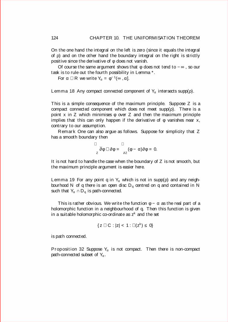
124 CHAPTER 10. THE UNIFORMISATION THEOREM
On the one hand the integral on the left is zero (since it equals the integralof ρ) and on the other hand the boundary integral on the right is strictlypositive since the derivative of φ does not vanish.
Of course the same argument shows that φ does not tend to −∞, so ourtask is to rule out the fourth possibility in Lemma *.
For α ∈ R we write Yα = φ−1(∞, α].
Lemma 18 Any compact connected component of Yα intersects supp(ρ).
This is a simple consequence of the maximum principle. Suppose Z is acompact connected component which does not meet supp(ρ). There is apoint x in Z which minimises φ over Z and then the maximum principleimplies that this can only happen if the derivative of φ vanishes near x,contrary to our assumption.
Remark One can also argue as follows. Suppose for simplicity that Zhas a smooth boundary then∫
Z∂φ ∧ ∂φ =
∫∂Z
(φ− α)∂φ = 0.
It is not hard to handle the case when the boundary of Z is not smooth, butthe maximum principle argument is easier here.
Lemma 19 For any point q in Yα which is not in supp(ρ) and any neigh-bourhood N of q there is an open disc Dq centred on q and contained in Nsuch that Yα ∩Dq is path-connected.
This is rather obvious. We write the function φ− α as the real part of aholomorphic function in a neighbourhood of q. Then this function is givenin a suitable holomorphic co-ordinate as zk and the set
z ∈ C : |z| < 1 : <(zk) ≤ 0
is path connected.
Proposition 32 Suppose Yα is not compact. Then there is non-compactpath-connected subset of Yα.

10.2. PROOF OF THE ANALOGUE OF THE MAIN THEOREM 125
Let D′ ⊂ D be an open interior disc whose closure lies in D and suchthat D′ contains the support of ρ. In our local coordinate about p we cantake D to correspond to |z| < 1 and D′ to |z| < r, for some finxed r < 1.Let C be the circle corresponding to |zvert = (1 + r)/2. It follows fromlem:obvious that we write the intersection Yα ∩ C as the union of finitelymany pieces C1, . . . CN say such that any two points in the same Cj can bejoined by a path in Yα \ D′. (We cover the compact set Yα ∩ C by finitelymany small discs of the form Dq considered in the Lemma.) Now consider thepath connected components of Yα \D′. Notice that by lem:obvious these arethe same as the connected components. If one of these is components is non-compact we are done. So suppose all these components are compact. SinceD′ has compact closure and Yα is not compact, there must be infinitely manydifferent compact components of Yα \ D′. The circle C divides X into twoconnected components one of which is a disc D′′ containing p. Any compactcomponent of Yα \D′ must either intersect the circle C or lie entirely withinthe disc D′′, for otherwise it lies in X \D′′ and gives a compact componentof Yα which does not meet supp(ρ). Contradicting Lemma *. The union ofthe components lying in D′′ is contained in a compact set—the closed discD′′. So there must be infinitely many different components which intersectC. But two of these must meet the same subset Cj and hence we get acontradiction since the points in Cj can be joined by paths in Yα \D′.
Putting together our results from this subsection we have
Proposition 33 Either φ tends to a finite limit at infinity in X, or thereare real numbers α < β and non compact, closed, path connected subsetsZα, Zβ ⊂ X such that φ(x) ≤ α for x ∈ Zα and φ(x) ≥ β for x ∈ Zβ.
10.2.3 The main argument
Our task now is to show that the second alternative of prop:summupmoredoes not occur, so we suppose it does and argue for a contradiction. Fixpoints xα ∈ Zα, xβ ∈ Zβ and a compact path-connected set Γ containing xαand xβ (for example the image of some path between the two points. Bylem:compeq there is no loss of generality in supposing that φi = φ on Γ.
Our preparations are now complete. For each i neither of the noncompactsets Zα, Zβ can be contained in the compact set supp(fi). Moreover they mustintersect a noncompact component of X \supp(fi) and by prop:oneend thereis only one such component. Thus there is a path in X \ supp(fi) joining

126 CHAPTER 10. THE UNIFORMISATION THEOREM
point yα of Zα to a point yβ of Zβ. Let γi : [0, 1]→ X be a loop in X startingand ending at xα of the following form:
• On the interval 0 ≤ t ≤ 1/4, γi traces out a path from xα to xβ in theset Γ.
• On the interval 1/4 ≤ t ≤ 1/2, γi traces out a path in Zβ from xβ toyβ.
• On the interval 1/2 ≤ t ≤ 3/4, γi traces out a path in X \supp(ρ) fromyβ to yα.
• On the interval 3/4 ≤ t ≤ 1, γi traces out a path in Zα from yα to xα.
Since X is simply connected this loop is contractible, so we can find acompact set Ki ⊂ X, containing the image of γi, such that γi is contractiblein Ki.
Now consider the smooth map F : X \R2 defined by
F (x) = (φ(x), φi(x)).
Then the composite F γ is a loop in R2 with the properties that
• For 0 ≤ t ≤ 1/4, F γ maps into the diagonal (x, x) in R2.
• For 1/4 ≤ t ≤ 1/2, F γ maps into the half plane (x1, x2) : x1 ≥ β.• For 1/2 ≤ t ≤ 3/4, F γ maps into the horzontal line (xi, ci).• For 3/4 ≤ t ≤ 1, F γ maps into the half-plane x1, x2) : x1 ≤ α.Let Z be the subset of R2 given by
Z = (x1, x2) : α < x1 < β,min(x1, ci) < x2 < max(x1, ci).
There are possible pictures for Z, depending whether c lies between α andβ , above β or below α. Howver it is elementary to see that in any case thearea satisfies
µ(Z) ≥ 1
4(β − α)2.
The conditions on our loop F γ imply that it does not meet Z. Now wehave

10.2. PROOF OF THE ANALOGUE OF THE MAIN THEOREM 127
Lemma 20 If P is any point of S the winding number of F γ around P isequal to ±1.
This is straightforward algebraic topology.
Corollary 8 F maps the compact set K ⊂ X onto Z.
This follows because if P is not in the image F (K) the composite of F with acontraction of γ would give a contraction of F γ in R2 \ P, contradictingthe homotopy invariance of the winding number.
Now we can apply prop:areabound to deduce that the integral of themodulus of the form F ∗i (dx1dx2) must be at least 1
4(β2−α2) = δ say. Writing
F ∗i (dx1dx2) = dφ ∧ dφiwe can state a conclusion to our preceding arguments as follows.
Corollary 9 If φ does not tend to a finite limit at infinity in X, then thereis some δ > 0 such that for each i∫
X|dφ ∧ dφi| ≥ δ.
Now we writedφ ∧ dφi = (dφ− dφi) ∧ dφi
and apply Lemma * from Chapter 5 to get∫X|dφ ∧ dφi| ≤ ‖dφ− dφi‖‖‖dφi‖,
but this tends to zero by cor:summup and we have the desired contradiction.