riemann surfaces - ut mathematics · 4 m392c (riemann surfaces) lecture notes thus,...
TRANSCRIPT
Riemann Surfaces
UT Austin, Spring 2016

M392C NOTES: RIEMANN SURFACES
ARUN DEBRAYMAY 6, 2016
These notes were taken in UT Austin’s M392C (Riemann Surfaces) class in Spring 2016, taught by Tim Perutz. Ilive-TEXed them using vim, so there may be typos; please send questions, comments, complaints, and corrections [email protected]. The image on the front cover is M.C. Escher’s Circle Limit III (1959), sourced fromhttp://www.wikiart.org/en/m-c-escher/circle-limit-iii. Thanks to Adrian Clough for finding a few typos.
Contents
1. Review of Complex Analysis: 1/20/16 32. Review of Complex Analysis, II: 1/22/16 53. Meromorphic Functions and the Riemann Sphere: 1/25/16 74. Analytic Continuation: 1/27/16 95. Analytic Continuation Along Paths: 1/29/16 126. Riemann Surfaces and Holomorphic Maps: 2/3/16 147. More Sources of Riemann Surfaces: 2/5/16 168. Projective Surfaces and Quotients: 2/8/16 189. Fuchsian Groups: 2/10/16 1910. Properties of Holomorphic Maps: 2/15/16 2111. The Riemann Existence Theorem: 2/22/16 2312. Normalizing Plane Algebraic Curves: 2/24/16 2413. The de Rham Cohomology of Surfaces: 2/26/16 2614. de Rham Cohomology in Degree 1: 2/29/16 2815. Poincaré Duality: 3/2/16 3116. Holomorphic 1-Forms: 3/4/16 3217. Hyperelliptic Riemann Surfaces: 3/7/16 3418. Elliptic Curves and Elliptic Functions: 3/9/16 3619. The j-invariant and Moduli of Elliptic Curves: 3/11/16 3820. The Euler Characteristic and the Riemann-Hurwitz Formula: 3/21/16 4021. Modular Curves: 3/23/16 4322. Modular Curves for Principal Congruence Subgroups: 3/25/16 4523. Euler Characteristics and Meromorphic 1-Forms: 3/28/16 4724. The Riemann-Roch Theorem: Background and Statement: 3/30/16 5025. : 4/1/16 5226. Modular Forms: 4/4/16 5227. Klein’s Quartic Curve: 4/6/16 5428. The Riemann-Roch Theorem: Towards a Proof: 4/8/16 5629. The Riemann-Roch Theorem: Exact Sequences of Sheaves: 4/11/16 5830. Serre Duality: 4/13/16 6131. Inverting the Laplacian: 4/15/16 6232. Inverting the Laplacian, II: 4/18/16 6533. Weyl’s Lemma: 4/20/16 6734. Uniformization: 4/22/16 6935. Uniformization, II: 4/25/16 71
2
Arun Debray May 6, 2016 3
36. Uniformization, III: 4/27/16 7337. Uniformization, IV: 4/29/16 7538. Uniformization, V: 5/2/16 7539. The Abel-Jacobi Map: 5/4/16 7740. The Abel-Jacobi Map, II: 5/6/16 78
Lecture 1.
Review of Complex Analysis: 1/20/16
Riemann surfaces is a subject that combines the topology of structures with complex analysis: a Riemannsurface is a surface endowed with a notion of holomorphic function. This turns out to be an extremely richidea; it’s closely connected to complex analysis but also to algebraic geometry. For example, the data of acompact Riemann surface along with a projective embedding specifies a proper algebraic curve over C, inthe domain of algebraic geometry.1 In fact, the algebraic geometry course that’s currently ongoing is veryrelevant to this one.
The theory of Riemann surfaces ties into many other domains, some of them quite applied: number theory(via modular forms), symplectic topology (pseudo-holomorphic forms), integrable systems, group theory, andso on: so a very broad range of mathematics graduate students should find it interesting.
Moreover, by comparison with algebraic geometry or the theory of complex manifolds, there’s very lowoverhead; we will quickly be able to write down some quite nontrivial examples and prove some deep theorems:by the middle of the semester, hopefully we will prove the analytic Riemann-Roch theorem, the fundamentaltheorem on compact Riemann surfaces, and use it to prove a classification theorem, called the uniformizationtheorem.
The course textbook is S.K. Donaldson’s Riemann Surfaces, and the course website is at http://www.ma.utexas.edu/users/perutz/RiemannSurfaces.html; it currently has notes for this week’s material, arapid review of complex function theory. We will assume a small amount of complex analysis (on the level ofCauchy’s theorem; much less than the complex analysis prelim) and topology (specifically, the relationshipbetween the fundamental group and covering spaces). Some experience with calculus on manifolds will behelpful. Some real analysis will be helpful, and midway through the semester there will be a few Hilbertspaces. Thus, though this is a topics course, the demands on your knowledge will more resemble a prelimcourse.
Let’s warm up by (quickly) reviewing basic complex analysis; the notes on the course website will delve intomore detail. For the rest of this lecture, G denotes an open set in C (from German gebiet, which commonlydenotes an open set).
The following definition is fundamental.
Definition 1.1. A function f : G→ C is holomorphic if for all z ∈ G, the complex derivative
f ′(z) = limh→0
f(z + h)− f(z)h
exists. The set of holomorphic functions G→ C is denoted O(G), after the Italian funzione olomorfa.
Even though it makes sense for this limit to be infinite, this is not allowed.First, let’s establish a few basic properties.• If H ⊂ G is open and f ∈ O(G), then f |H ∈ O(H).• The sum, product, quotient, and chain rules hold for holomorphic functions, so O(G) is a commutativering (with multiplication given pointwise) and in fact a commutative C-algebra.2
In other words, holomorphic functions define a sheaf of C-algebras on G.By a rephrasing of the definition, then if f is holomorphic on G, then it has a derivative f ′ on G, i.e. for all
z ∈ G, one can write f(z + h) = f(z) + f ′(z)h+ εz(h), where εz(h) ∈ o(h) (that is, εz(h)/h→ 0 as h→ 0).
1This sentence is packed with jargon you’re not assumed to know yet.2A C-algebra is a commutative ring A with an injective map C → A, which in this case is the constant functions.
4 M392C (Riemann Surfaces) Lecture Notes
Thus, a holomorphic function is differentiable in the real sense, as a function G → R2. This means thatthere’s an R-linear map Dzf : C→ C such that f(z + h) = f(z) + (Dzf)(h) + o(h): here, Dzf(h) = f ′(z)h.
However, we actually know that Dzf is C-linear. This is known as the Cauchy-Riemann condition. Sinceit’s a priori R-linear, saying that it’s C-linear is equivalent to it commuting with multiplication by i. Dzf isrepresented by the Jacobian matrix
Dzf =[∂u∂x
∂u∂y
∂v∂x
∂v∂y
].
A short calculation shows that this commutes with i iff the following equations, called the Cauchy-Riemannequations, hold:
(1.2) ∂u
∂x= ∂v
∂yand ∂u
∂y= −∂v
∂x.
The content of this is exactly that Dzf is complex linear.Conversely, suppose f : G→ C is differentiable in the real sense. Then, if it satisfies (1.2), then Dzf is
complex linear. But a complex linear map C→ C must be multiplication by a complex number f ′(z), so f isholomorphic, with derivative f ′.
Power Series. The notation D(c,R) means the open disc centered at c with radius R, i.e. all points z ∈ Csuch that |z − c| < R.
Definition 1.3. Let A(z) =∑∞n=0 an(z − c)n be a C-valued power series centered at a c ∈ C. Then, its
radius of convergence is R = sup|z − c| : A(z) converges, which may be 0, a positive real number, or ∞.
Theorem 1.4. Suppose A(z) =∑n≥0 an(z − c)n has radius of convergence R. Then:
(1) R−1 = lim sup|an|1/n;(2) A(z) converges absolutely on D(c,R) to a function f(z);(3) the convergence is uniform on smaller discs D(c, r) for r < R;(4) the series B(z) =
∑n≥1 nan(z− c)n−1 has the same radius of convergence R, so converges on D(c,R)
to a function g(z); and(5) f ∈ O(D(c,R)) and f ′ = g.
These aren’t extremely hard to prove: the first few rely on various series convergence tests from calculus,though the last one takes some more effort.
Paths and Cauchy’s Theorem. By a path we mean a continuous and piecewise C1 map [a, b] → C forsome real numbers a < b. That is, it breaks up into a finite number of chunks on which it has a continuousderivative. A loop is a path γ such that γ(a) = γ(b).
If γ is a C1 path in G (so its image is in G) and f : G→ C is continuous, we define the integral∫γ
f =∫γ
f(z) dz :=∫ b
a
f(γ(t))γ′(t) dt.
This is a complex-valued function, because the rightmost integral has real and imaginary parts. This makessense as a Riemann integral, because these real and imaginary parts are continuous. This is additive on thejoin of paths, so we can extend the definition to piecewise C1 paths. Moreover, integrals behave the expectedway under reparameterization, and so on.
Theorem 1.5 (Fundamental theorem of calculus). If F ∈ O(G) and γ : [a, b]→ G is a path, then∫γ
F ′(z) dz = F (γ(b))− F (γ(a)).
This is easy to deduce from the standard fundamental theorem of calculus. In particular, if γ is a loop,then the integral of a holomorphic function is 0.
Now, an extremely important theorem.
Definition 1.6. A star-domain is an open set G ⊂ C with a z∗ ∈ G such that for all z ∈ G, the line segment[z∗, z] joining z∗ and z is contained in G.
For example, any convex set is a star-domain.

2 Review of Complex Analysis, II: 1/22/16 5
Theorem 1.7 (Cauchy). If G is a star-domain, γ is a loop in G, and f ∈ O(G), then∫γf = 0. Indeed,
f = F ′, where
F (z) =∫
[z∗,z]f.
The proof is in the notes, but the point is that you can check that this definition of F produces aholomorphic function whose derivative is f ; then, you get the result. The idea is to compare F (z + h) andF (z) should be comparable, which depends on an explicit calculation of an integral of a holomorphic functionaround a triangle, which is not hard.
Cauchy didn’t prove Cauchy’s theorem this way; instead, he proved Green’s theorem, using the Cauchy-Riemann equations. This is short and satisfying, but requires assuming that all holomorphic functions areC1. This is true (which is great), but the standard (and easiest) way to show this is. . . Cauchy’s theorem.
Lecture 2.
Review of Complex Analysis, II: 1/22/16
Today, we’re going to continue not being too ambitious; next week we will begin to geometrify things. Lasttime, we stopped after Cauchy’s theorem for a star domain G: for all f holomorphic on G and loops γ ∈ G,∫γf = 0, and in fact one can write down an antiderivative for f , and then apply the fundamental theorem of
calculus.Then one can bootstrap one’s way up to a more powerful theorem; the next one is a version of the
deformation theorem.
Corollary 2.1 (Deformation theorem). Let G ⊂ C be open and γ0, γ1 : [a, b] ⇒ G be C1 loops that are C1
homotopic through loops in G. Then, for all f ∈ O(G),∫γ0f =
∫γ1f .
Proof sketch. Fix a C1 homotopy Γ : [a, b]× [0, 1]→ G such that Γ(a, s) = Γ(b, s) for all s, γ0(t) = Γ(t, 0),and γ1(t) = Γ(t, 1). Then, it is possible to divide [a, b]× [0, 1] into a grid of rectangles fine enough such thatthe image of each rectangle is mapped under Γ to a subset of G contained in an open disc in C, as in Figure 1.Now, by Cauchy’s theorem in a disc, the integral does not depend on path within each disc, so we can apply
a b0
1
Figure 1. Subdividing [a, b]× [0, 1] into rectangles.
Γ in over the rectangles from 0 to 1, showing that the two integrals are the same.
Corollary 2.2. Cauchy’s theorem holds in any simply connected open G ⊂ C.
This is considerably more general than star domains (e.g. the letter C is simply connected, but not a stardomain). Moreover, on such a domain, any f ∈ O(G) has an antiderivative: pick some basepoint z0 ∈ G, andlet γ(z0, z) be a path from z0 to z. Then,
F (z) =∫γ(z0,z)
f(z) dz
is well-defined, because any two choices of path differ by the integral of a holomorphic function on a loop,which is 0.
We can also use this to understand power series representations.

6 M392C (Riemann Surfaces) Lecture Notes
Proposition 2.3 (Cauchy’s integral formula). , Let G be a domain in C containing the closed disc D. Iff ∈ O(G), then
f(z) = 12πi
∫∂D
f(w)w − z
dw.
Proof idea. Suppose D is centered at z and has radius R, and let C(z, r) denote the circle centered at z andwith radius r. We’ll also let D∗ denote the punctured disc, i.e. D minus its center point. By calculating∫γ
dz/z = 2πi, one has that
12πi
∫∂D
f(w)z − w
dw − f(z) = 12πi
∫∂D
f(w)− f(z)w − z
dw.
Using Corollary 2.1, for r ∈ (0, R),
= 12πi
∫C(z,r)
f(w)− f(z)w − z
dw,
and as r → 0, this approaches f ′(z), which is bounded, and the integral over smaller and smaller circles of abounded function tends to zero.
Theorem 2.4 (Holomorphic implies analytic). If D is a disc centered at c and f ∈ O(D), then on that disc,
f(z) =∑n≥0
an(z − c)n, where an = 12πi
∫∂D
f(z)(z − c)n+1 dz.
Proof sketch. For any z ∈ D, there’s a δ > 0 such that the closed disc D(z, δ) of radius δ is contained in D.Hence, by Proposition 2.3,
f(z) = 12πi
∫C(z,δ)
f(w)w − z
dw
=∫C(c,R′)
f(w)w − z
dw
for any R′ ∈ (0, δ), by Corollary 2.1. We’d like to force a series on this. First, since
1w − z
= 1(w − c)− (z − c) = 1
w − c
(1
1− z−cw−c
),
then
f(z) = 13πi
∫C(c,R′)
f(w)w − c
11− z−c
w−cdw
= 12πi
∮f(w)w − c
∑n≥0
(z − c)n
(w − c)n dw.
Since |(z − c)/(w − c)| < 1 on C(c,R′), then this is well-defined, and since it’s a geometric series, it has niceconvergence properties, and so we can exchange the sum and integral to obtain
=∑n≥0
12πi
(∮f(w)
(w − c)n+1 dw)
︸ ︷︷ ︸an
(z − c)n.
One application of this is to understand zeros of holomorphic functions. If f ∈ O(G) and f(c) = 0, then letf(z) =
∑an(z− c)n be its power series and am be the first nonzero coefficient. Then, in a neighborhood of c,
f(z) = (z − c)m∑n≥m
an(z − c)n−m︸ ︷︷ ︸g(z)
.
This g is holomorphic and does not vanish on this neighborhood, so the takeaway is f(z) = (z − c)mg(z) nearc, with g holomorphic and nonvanishing. This m is called the multiplicity, denoted mult(f, c). In particular,if f(c) 6= 0, then m = 0.

3 Review of Complex Analysis, II: 1/22/16 7
Theorem 2.5. If G is a connected open set and f ∈ O(G) is not identically zero, then f−1(0) is discrete inC.
Proof. If f(c) = 0, then there’s a disc D on which f(z) = (z − c)mg(z), where m ≥ 1 and g is nonvanishing,so the only place f can vanish on D (i.e. near c) is at c itself.
Definition 2.6. A function f ∈ O(C), so holomorphic on the entire plane, is called entire.
Theorem 2.7 (Liouville). A bounded, entire function is constant.
Proof sketch. We’ll show that f ′(z) = 0 everywhere. By Proposition 2.3, we know
f ′(z) = 12πi
∫C(z, r) f(w)
(w − z)2 dw,
and we can deform this loop to C(0, R). Then, one bounds the integral, and the bound ends up being O(1/R),so as R→∞, this necessarily goes to 0.
Lecture 3.
Meromorphic Functions and the Riemann Sphere: 1/25/16
We’re still going to be doing classical function theory today, but we’re going to begin to geometrify it.Recall that G ⊂ C denotes an open set.
We’ll begin with the following theorem.
Theorem 3.1 (Morera). Let f : G→ C be a continuous function such that for all triangles T ⊂ G,∫∂Tf = 0.
Then, f is holomorphic.
This is surprisingly easy to prove, given what we’ve done.
Proof. Since holomorphy is a local property, we may without loss of generality work on a disc D(z0, r) ⊂ G.Then, define F : D(z0, r) → C by F (z) =
∫[z0,z] f ; using the hypothesis on triangles, F ′ = f . Thus, as we
showed last time, this means F ∈ O(G), and so it’s analytic, and therefore it has derivatives of all orders.Thus, F ′ = f is holomorphic.
This is useful, e.g. one may have a function which is defined through an improper integral, or a pointwiselimit of holomorphic functions. Then, Morera’s theorem allows for an easier, indirect way to show holomorphy.Here’s another application.
Definition 3.2. If z0 ∈ G, a function f ∈ O(G \ z0) has a removable singularity at z0 if f can be extendedholomorphically to G.
Theorem 3.3. Suppose f ∈ O(G \ z0) and |f | is bounded near z0. Then, f has a removable singularity atz0.
There are several ways to prove this quickly.
Proof. We can without loss of generality translate this to the origin, so assume z0 = 0. If g(z) = zf(z), theng(z)→ 0 as z → 0, since |f(z)| is bounded in a neighborhood of the origin. Thus, g extends continuously toall of G, with g(0) = 0.
Next, one should check that Morera’s theorem applies to g; the only nontrivial example is a triangle aroundthe origin. However, since g is holomorphic everywhere except at 0, the deformation theorem allows us toshrink the triangle as much as we want, and since g → 0, the integral goes to 0 as well. If the triangle’s edgeor vertex touches the origin, one can use the deformation theorem to push it away again.
In particular, g is holomorphic on G and has a zero at 0, so by the discussion on multiplicities last time,g(z) = z · f(z), where f is holomorphic on all of G; this produces our desired extension of f .
Definition 3.4.• If z0 ∈ G and f ∈ O(G \ z0), then f has a pole at z0 if there’s an m ∈ N such that (z − z0)mf(z)is bounded near z0 (and hence has a removable singularity there). The least such m is called theorder of the pole.

8 M392C (Riemann Surfaces) Lecture Notes
• A meromorphic function on G is a pair (∆, f) consisting of a discrete subset ∆ ⊂ G and anf ∈ O(G \∆) such that f has a pole at each z ∈ ∆.
So, nothing worse than a pole happens for a meromorphic function. There are essential singularities, whichare singularities which aren’t poles, but we will not discuss them extensively; almost everything in sight willbe meromorphic.
The Riemann Sphere. In some sense, the Riemann sphere is the most natural setting for meromorphicfunctions, and the first nontrivial example of a Riemann surface (still to be defined).
Definition 3.5. The Riemann sphere C = C ∪ ∞ is the one-point compactification of C, so its topologyhas as its open sets (1) opens in C, and (2) (C \K) ∪ ∞, where K ⊂ C is compact.
There is a homeomorphism φ : C → S2 = (x, y, z) ∈ R3 | x2 + y2 + z2 = 1 given by stereographicprojection: send∞ 7→ (0, 0, 1) (the north pole), and then any other z ∈ C defines a line from z in the xy-planeto (0, 0, 1) intersecting S2 at one other point; this is φ(z). Hence, we will use C and S2 interchangeably.
Figure 2. Depiction of stereographic projection, where N = (0, 0, 1) is the north pole.Source: http://www.math.rutgers.edu/~greenfie/vnx/math403/diary.html.
Definition 3.6. A continuous map f : G→ S2 is holomorphic if for all z ∈ G, either• f(z) ∈ C (so it doesn’t hit ∞) and f : G→ C is holomorphic, or• if f(z) ∈ C \ 0, then 1/f(w) : G→ C is holomorphic, where 1/∞ is understood to be 0.
If the image of f contains neither 0 not ∞, then both criteria hold, and are equivalent (since 1/z isholomorphic on any neighborhood not containing zero).
Proposition 3.7. The meromorphic functions on G can be identified with the holomorphic functions G→ S2.
Proof. Suppose f is meromorphic on G, so that it has a pole of order m at z0. Then, f(z) = (1/(z−z0)m)g(z)for some holomorphic g with a removable singularity at z0, and g(z0) 6= 0.
By letting 1/0 = ∞, this realizes f as a continuous map G → S2, and 1/f = (z − z0)m(1/g), which iscertainly holomorphic near z0, so f is holomorphic as a map to S2.
The converse is quite similar, a matter of unwinding the definitions, but has been left as an exercise.
You can also define a notion of a holomorphic function coming out of S2, not just into.
Definition 3.8. Let G ⊂ S2 be open. A continuous f : G→ S2 is holomorphic if one of the following is true.• If ∞ 6∈ G, then we use the same definition as above.• If ∞ ∈ G, then it’s holomorphic on G \∞ and there’s a neighborhood N of ∞ in G such that thecomposition
N−1 z 7→1/z // Nf // S2
is holomorphic.
If you’re used to working with manifolds, this sort of coordinate change is likely very familiar: every timewe talk about ∞, we take reciprocals and talk about 0.
Example 3.9. Every rational function p ∈ C(z) is meromorphic, and extends to a holomorphic map S2 → S2.

4 Meromorphic Functions and the Riemann Sphere: 1/25/16 9
Figure 3. A depiction of the map z 7→ z2 on the Riemann sphere, which fixes the poles.Source: https://en.wikipedia.org/wiki/Degree_of_a_continuous_mapping.
Now, we can talk about these geometrically: z 7→ z2 sends einθ 7→ e2inθ, so it doubles the longitude(modulo 1). In particular, it wraps the sphere twice around itself, preserving 0 and ∞, as in Figure 3.Example 3.10. A Möbius map is a map
µ(z) = az + b
cz + d,
where a, b, c, d ∈ R and ad− bc = 1. This extends to a holomorphic map S2 → S2 with a holomorphic inverse(the Möbius map associated to
[a bc d
]−1). Thus, there’s a homeomorphism SL2(R)/±I to the group ofMöbius transformations.
One interesting corollary is that the point at infinity is not special, since there’s a Möbius map sending itto any other point of S2, and indeed they act transitively on it. So we don’t really have to distinguish thepoint at infinity from this geometric point of view.Theorem 3.11. If f : S2 → S2 is holomorphic, then it’s a rational function. In particular, the Möbius mapsare the only invertible holomorphic maps S2 → S2.
The idea is to eliminate the zeros and poles by multiplying by (z − z0)m; then, one can apply Liouville’stheorem to show that the result is constant.
Lecture 4.
Analytic Continuation: 1/27/16
This corresponds to §1.1 in the textbook, and is one of the classical motivations for Riemann surfaces.The problem is: if G ⊂ C is open and f ∈ O(G), then we would like to extend f holomorphically, or
maybe meromorphically, to a larger domain H ⊃ G. Such extensions are called analytic (resp. meromorphic)continuations of f .3
Remark. If H is connected, then there exists at most one meromorphic continuation of f to H, because thedifference of two continuations vanishes on the open set G, and hence vanishes everywhere.Example 4.1. Let f(z) =
∑n≥0 z
n, which converges on the open unit disc, but diverges when |z| ≥ 1. Atfirst sight, this suggests we’ll never get any farther than the disc, but this turns out to merely be an artifactof this presentation of f : we could instead write it as f(z) = 1/(1− z), which meromorphically extends f tothe whole of C (with a single pole at z = 1). Thus, this power series representation is not per se intrinsic.
One can take this further and define analytic continuations of general functions defined by power series.Example 4.2. This example is more sophisticated, and will take longer; it reflects a common theme in thissubject, that the examples are nontrivial and are worth taking seriously. Define the Γ-function
Γ(z) =∫ ∞
0tz−1e−t dt
3Though “holomorphic continuation” would make more sense, tradition gives us the term “analytic continuation.”

10 M392C (Riemann Surfaces) Lecture Notes
on the open set Re z > 0. This integral is doubly improper, since there’s a singularity at 0 and it’s unboundedon the right, so we really should rewrite it as
Γ(z) = limε→0+
∫ 1
ε
tz−1e−t dt+ limT→∞
∫ T
1tz−1e−t dt.
Let Ha = z | Re z > a. We’re going to show that Γ extends to the entire plane, but first we need to showthat it’s holomorphic on the right half-plane.Proposition 4.3. Γ ∈ O(H0).Proof sketch. Since we need to realize Γ(z) as a limit, let
gn(z) =∫ n
1/ntz−1e−t dt.
This is an integral of a holomorphic function, so gn ∈ O(C) and
g′n(z) =∫ n
1/n
∂
∂z
(tz−1e−t
)dt = (z − 1)gn(z − 1).
If a > 0, then g converges uniformly on the strip a < Re z < b — the goal is to show that gn is uniformlyCauchy on this strip (the details of which are left to the reader) by comparing to the integral of e−t/2 fort 0, the point being that ex−1e−t ≤ e−t/2 for t sufficiently large. For t < 1, one should compare it to theintegral of tx−1. Then, we need to use the following theorem.Theorem 4.4. If fn ∈ O(G) and fn(z)→ f(z) locally uniformly, then f ∈ O(G).
The proof uses Morera’s theorem (Theorem 3.1) and can be found in the review notes (or Rudin, etc.). Inany case, this means Γ = limn→∞ gn is holomorphic on the right half-plane.
Now, we can talk about extending Γ.Theorem 4.5. Γ has a meromorphic continuation to C, whose only poles are simple poles4 at 0, −1, −2,and so on.Proof. Since the gamma function is given by an integral, let Γ0 be that integral from 0 to 1, and Γ∞ bethe integral from 1 to ∞. Then, the argument above shows that Γ∞ ∈ O(C), so the only extension that weactually need to make is of
Γ0(z) =∫ 1
0tz−1e−t dt.
The cunning idea is that we’re going to look at the nth-order Taylor polynomial for e−t, which provides anintegral we can actually do, and then treat everything else separately. Specifically, let
en(t) =n−1∑j=0
(−t)j
j! ,
so that
Γ0(z) =∫ 1
0tz−1(e−t − en(t)
)dt︸ ︷︷ ︸
Γn(z)
+∫ 1
0tz−1en(t) dt.
= Γn(z) +n−1∑j=0
(−1)j
j!(z + j) .
The (z + j) in the denominator on the right gives us simple poles at 0,−1,−2, . . . ,−n+ 1. But e−t − en(t)has a zero of order n at t = 0, so ∫ 1
0tz−1(e−t − en(t)
)dt
exists on H−n, so Γn ∈ O(H−n). Thus, we can extend Γ meromorphically to all of C, because any z ∈ C isin some H−n, so we can work this with Γn.
4A pole is simple if it’s degree 1.

4 Analytic Continuation: 1/27/16 11
It goes without saying that Γ is one of the most prominent functions in analytic number theory.
These two successful examples of meromorphic continuation are in some sense atypical; in general, there isa problem of multi-valuedness or monodromy.
Example 4.6. For an algebraic example of this problem, consider
f(z) =∑n≥0
(1/2n
)zn,
where (α
n
)= α(α− 1)(α− 2) · · · (α− n+ 1)
n! .
By a generalized binomial theorem (or checking that it satisfies the right differential equation), one canshow that f converges on D(0, 1) to a branch of
√1 + z. We can extend holomorphically to the cut plane
C \ (−∞,−1] by writing f(z) = exp((1/2) log(1 + z)), where we can choose a branch of log(1 + z) in this cutplane, such as log(reiθ) = log r + iθ, with θ ∈ (−π, π).
There’s nothing particularly special about this branch cut. Plenty of other branch cuts (paths from −1 to−∞ whose complements are simply connected) work just as fine — but we cannot extend further, because aswe go around a loop around −1, f(z) flips −f(z) (the other branch of
√1 + z), since the logarithm changes
by 2πi. This is a little unsatisfactory, since we can’t go further.
A similar story holds for just about any algebraic function, since one has to take a branch cut to resolvethe ambiguity of multiple roots.
The Riemann surfaces way to approach this is instead of making arbitrary branch cuts, it’s more canonicalinstead to study the equation w2 − (1− z) = 0, which implicitly defines w as a square root of 1 + z. Then,we consider the set
X = (z, w) ∈ C2 | P (z, w) = 0,
where P (z, w) = w2 − (1 + z). Soon, we will see that this X is a Riemann surface. We can play exactlythe same game with any P (z, w) : C2 → C that is holomorphic in each variable separately, including anypolynomial in z and w. This defines for us its zero set X = P (z, w) = 0.
Then, we have an implicit function theorem, which is a major classical motivation for the theory ofRiemann surfaces, just as the implicit function theorem on Rn is a major classical motivation for definingabstract manifolds.
Theorem 4.7 (Implicit function theorem). If (z0, w0) ∈ X and ∂P∂w (z0, w0) 6= 0, then there’s a disc D1 ⊂ C
centered at z0 ∈ C and a disc D2 ⊂ C centered at w0, and a holomorphic φ : D1 → D2 such that φ(z0) = w0and X ∩ (D1 ×D2) is the graph of φ, i.e. (z, φ(z)) | z ∈ D1.
An analogue of this function holds for C1 real functions (or C∞ ones), and this version can be extractedfrom that, but it has a simpler, direct proof.
Proof. This proof hinges on a theorem called the argument principle, that if f ∈ O(G) and D is a closed discin G with f(z) 6= 0 on ∂D, then
(4.8) 12πi
∫∂D
f ′(w)f(w) dw =
∑z∈Df(z)=0
mult(f ; z).
That is, integrating the logarithmic derivative counts the zeros inside D, with multiplicity. There’s also therelated formula
(4.9) 12πi
∫∂D
wf ′(w)f(w) dw =
∑z∈Df(z)=0
zmult(f ; z).
These are nice exercises in residue calculus.

12 M392C (Riemann Surfaces) Lecture Notes
Returning to the implicit function theorem, let fz = P (z, ·), so fz0(w0) = 0, but f ′z0(w0) 6= 0. Thus,
mult(fz0 ;w0) = 1, and therefore by isolation of zeros, there’s a disc D2 centered at w0 such that w0 is theonly zero of fz0 in D2. Hence, by (4.8),
12πi
∫∂D2
f ′z0
fz0
= 1.
Since fz0 6= 0 on the boundary, then there’s a δ > 0 such that |fz0 | > 2δ > 0 on ∂D2. Thus, there’s a disc D1centered at z0 such that for all z ∈ D1, |fz| > δ on ∂D2 because P is continuous. Hence,
12πi
∫∂D2
f ′zfz
= 1,
or, by (4.8), there’s a unique solution w = φ(z) to P (z, w) = 0 with z ∈ D1 and w ∈ D2. Thus, we need onlyto show that φ is holomorphic. By (4.9),
φ(z) = 12πi
∫∂D2
wf ′z(w)fz(w) dw = 1
2πi
∫∂D2
w
P (z, w)∂P
∂w(z, w) dw.
Hence, φ is holomorphic in z (since its derivative is given by differentiating under the integral sign).
Thus, even working just with zero sets of algebraic functions, Riemann surfaces show up very nicely.
Lecture 5.
Analytic Continuation Along Paths: 1/29/16
Today, we’re going to talk about analytic continuation along paths and the interesting things that result.There’s also a more classical Weierstrass way to look at this.
Definition 5.1. If φ is a holomorphic function defined on a neighborhood U of a z0 ∈ C and γ : [0, 1]→ Cis a path with γ(0) = z0, then an analytic continuation of φ along γ consists of a pair (Ut, φt) for all t ∈ [0, 1],where Ut is a neighborhood of γ(t) and φt ∈ O(Ut) such that:
• φ0 = φ on U0 ∩ U , and• the different φt should agree, in the sense that for all s ∈ [0, 1], there’s a δ > 0 such that if |t− s| < δ,then φs and φt agree on Us ∩ Ut.
γ
z0
Figure 4. Analytic continuation along a path; on sufficiently close circles, the extensionsmust agree.
Note, however, that if γ intersects itself, then there’s no requirement for the extensions to agree on thoseoverlaps (if δ is sufficiently small, for example). Weierstrass said this is how one should think of complexanalytic functions, and this confused a lot of people, but did lead to Weyl’s work that we’ll discuss in a fewlectures.
Example 5.2. The logarithm is a very good example. Start with a branch of log defined on some open setU0, so log(reiθ) = log r + iθ, or log z = log|z|+ i arg z, for some continuous, real-valued arg : U0 → R/2πZ.
Then, for any γ : [0, 1] → C∗ with γ(0) = z0 ∈ U0, we can uniquely lift arg γ : [0, 1] → R/2πZ to Rconsistent with arg(z0); this lift will be called argγ .5 Then, define logγt(z) = log|z|+ argγ(t)(z), which definesa continuation of the logarithm around γ.
5One can think of this in terms of the theory of covering spaces, which is one reason this function lifts.

5 Analytic Continuation Along Paths: 1/29/16 13
Example 5.3. For a more algebraic example, let
φ(z) =∑j≥0
(1/2j
)zj
on the unit disc D(0, 1), so φ(z)2 = z + 1. Then, one can continue along any γ with image in C \ −1 bysetting φt(z) = exp((1/2) logγt(1 + z)). However, if γ(t) = −1 + e2πit, then γ winds around −1, and when itreturns to a point, the extension of φ has a different value!
Example 5.4. Analytic continuation along paths works particularly well with differential equations: let pand q be meromorphic functions. Then, we want to find a u(z) such that u′′ + p(z)u′ + q(z)u = 0, which we’llcall p, q .6 If you think differential equations are boring, questions like these are still motivated by study ofD-modules and the like in algebraic geometry.
Let’s work near a point z0 where p and q are holomorphic, so z0 is a regular point, and without loss ofgenerality make z0 = 0. We’re going to look for series solutions: set p(z) =
∑n≥0 pnz
n and q(z) =∑qnz
n
on D(0, R) for some R, and we want to find u(z) =∑n≥0 unz
n. Equating the coefficients of zn in p, q , oneobtains the recurrence relation
(n+ 1)(n+ 2)un+1 +n∑i=0
(n+ i− 1)piun+1−i +n∑j=0
qjun−j = 0.
By induction, one shows that all of the uj are determined by a choice of (u0, u1) ∈ C2.
Proposition 5.5.∑unz
n converges in the same disc D(0, R).
The detailed proof is a homework assignment, and depends on the following lemma, due to an idea ofCauchy.
Lemma 5.6 (Majorization). Say |pn| ≤ Pn and |qn| ≤ Qn. Then, let P (z) =∑Pnz
n and Q(z) =∑Qnz
n.If u =
∑unz
n is a solution to p, q and Un =∑Unz
n is a solution to P,Q , and if U0 = |u0| and U1 = |u1|,then |un| ≤ |Un|.
The proof involves some straightforward estimates after the recurrence formula.
Proof sketch of Proposition 5.5. Let’s work on D(0, r) where r < R. Then, we have estimates like |pn| ≤M/rn and |qn| ≤M/rn, where M = sup
z∈D(0,r)|p(z)|, |q(z)|, which follows from Cauchy’s estimates (whichthemselves are corollaries of the Cauchy integral formula, Proposition 2.3).
Now, using the majorization lemma, we can compare p, q to
∑n≥0|pn|zn,
∑n≥0|qn|zn and
∑M
rnzn,∑M
rnzn .
It makes sense to compare this to M/(1− z/r),M/(1− z/r)2 , i.e. the equation
u′′ + Mu′
1− z/r + Mu
(1− z/r)2 = 0.
This last equation has an explicit solution µ/(1 − z/r) for some µ, and its Taylor series converges onD(0, r); now, using the majorization lemma, the coefficients of our original series are smaller, and therefore itconverges.
Thus, we have a 2-dimensional C-vector space V of solutions near z0. The tie-in to the rest of lecture isthe following proposition/exercise.
Exercise 5.7. Show that if p, q ∈ O(G) and γ : [0, 1]→ G, then any solution to p, q has a solution along γthrough solutions to p, q .
6“If you’re typing notes, feel free to call it something else, like Lp.q .”

14 M392C (Riemann Surfaces) Lecture Notes
Monodromy. If γ is now a loop in G, so γ(0) = γ(1) = z0, then analytic continuation around γ defines alinear map Mγ : V → V called the monodromy map: you go around and end up not where you started, andit’s easy to see that this dependence is linear.
Exercise 5.8. Mγ depends only on the homotopy class of γ (relative to basepoints).
Thus, this is only interesting if G isn’t simply connected, so in general we get interesting examples ofmonodromy by going around poles of p and q. In particular, there’s the oxymoronic-sounding notion ofregular singular points. The prototype is the following, simpler equation:
(5.9) u′′ + A
zu′ + B
z2u = 0,
where A,B ∈ C are just constants. We seek solutions of the form u(z) = zα, where α ∈ C; this is definedinitially near 1, and then analytically continued along paths in C∗. If you write down the left-hand side, youend up getting
u′′ + A
zu′ + B
z2u = (α(α− 1) +Aα+B)︸ ︷︷ ︸I(α)
zα−2.
In other words, to get a solution, we need I(α) = 0; this is called the indicial equation. Since it’s a quadratic,then there’s one or two roots: if the roots α1 and α2 are distinct, then (zα1 , zα2) is a basis for V (the solutionsnear 1), and if γ is the unit circle, then the monodromy matrix in this basis is
(5.10) Mγ =[e2πiα1 0
0 e2πiα2
].
If α is a related root, the basis we get is (zα, zα log z), and the monodromy matrix is a nontrivial Jordanblock:
Mγ = e2πiα[1 2πi0 1
].
One takeaway is that even an equation as simple as (5.9) has monodromy.This generalizes quite naturally.
Definition 5.11. A z0 ∈ C is a regular singular point of u′′ + pu′ + qu = 0 if p has a pole of order at most 1and q has a pole of order at most 2 at z0.
One seeks solutions via the Frobenius method: since p has a simple pole and q has a double pole, thenthere are p, q holomorphic in a neighborhood of 0 such that p(z) = A/z + p(z) and q(z) = B/z2 +C/z + q(z).Thus, the indicial equation is α(α− 1) +Aα+B = 0.
Proposition 5.12. If there are indicial roots α1 and α2 such that α1 − α2 6∈ Z, then there are solutionsu1, u2 ∈ V such that u1 = zα1w1 and u2 = zα2w2, and the monodromy matrix is as in (5.10).
Lecture 6.
Riemann Surfaces and Holomorphic Maps: 2/3/16
Today, we’ll begin with section 3.1 of the book, defining Riemann surfaces properly. This may be veryroutine to you or far from it; in any case, the notion of a manifold is central to mathematics, and now’s asgood a time as any to see it.
Definition 6.1. A Riemann surface (abbreviated R.S.) is the data of• a Hausdorff topological space X, along with• an atlas; that is, a collection (Uα, φα) | α ∈ A where the Uα ⊂ X are open,
⋃α∈A Uα = X, and
φα : Uα → C is a homeomorphism onto its image;7 we require that for all α, β ∈ A, the transitionmap ταβ = φβ φ−1
α : φα(Uα ∩ Uβ)→ C is holomorphic.We deem two atlases on X to define the same surface if their union is also an atlas satisfying the aboveconditions.
The rest of this week will be devoted to examples of Riemann surfaces, and unwinding this definition.
7Each pair (Uα, φα) is called a chart.

6 Riemann Surfaces and Holomorphic Maps: 2/3/16 15
X
Uα
φα
Uβ
ψα
φα(Uα) φα(Uβ)
ταβ
Figure 5. A transition map between charts for a Riemann surface X.
Remark.• If p ∈ Uα, we can think of φα as defining a holomorphic coordinate z neat p on X. The definitionforces us to work only with notions that are independent of the particular coordinate we chose; forexample, it does make sense to ask for a holomorphic function’s order of vanishing at p.
• There are many variants of this definition of a Riemann surface given by replacing holomorphicitywith something else. If one instead requires the maps to be smooth, the resulting definition is for asmooth surface; if we require smoothness with positive Jacobian, it’s a smooth oriented surface; andmany more.
• A C-linear map C→ C has non-negative Jacobian, because the map C→ C sending z 7→ az acts onR2 by
[Re a − Im aIm a Re a
], which has det |a|2. In particular, a Riemann surface is also a smooth oriented
surface. Thus, by the classification of compact, smooth, oriented surfaces, any connected, compactRiemann surface is equivalent to a standard genus-g surface.
• In the conventional definition of smooth surfaces, one generally assumes that a smooth surface has acountable atlas; equivalently, one may take the space to be paracompact or second-countable. Thereare tricky counterexamples if you don’t include this (e.g. they do not admit partitions of unity, andhence Riemannian metrics). However, this isn’t necessary in the world of Riemann surfaces.
Theorem 6.2 (Radó). Any connected Riemann surface has a countable holomorphic atlas.
Thus, unlike in differential geometry, where we care only about nicer surfaces, here we get that our surfacesare nice already.8
Now, we want to know not just what these are, but also how to map between them.
Definition 6.3. Let (X, (Uα, φα)) and (Y, (Vβ , ψβ)) be Riemann surfaces. Then, a holomorphic mapf : X → Y is a continuous map such that for all charts φα and ψβ , ψβ f φ−1
β is holomorphic. An invertibleholomorphic map is called biholomorphic.
Courtesy of the implicit function theorem for holomorphic functions, Theorem 4.7, the inverse of abiholomorphic function is also holomorphic.
Example 6.4.(1) Any open set Ω ⊂ C is a Riemann surface with just one chart φ : Ω→ C given by inclusion (the only
translation functions are the identity, which is holomorphic).
8Later in the class, we’ll prove the uniformization theorem, which says that every connected Riemann surface is equivalent toa quotient of C, the sphere, or the hyperbolic plane by a group action. This implies Radó’s theorem, but is now how Radóoriginally proved it.

16 M392C (Riemann Surfaces) Lecture Notes
(2) The Riemann sphere S2 = C is a Riemann surface with an atlas of two charts: the copy of C inside Cis sent to C by the identity, and C∗ ∪ ∞ is sent to C by z 7→ 1/z; the transition map is z 7→ 1/z onC∗, which is holomorphic. The Möbius maps µ : S2 → S2 given by µ(z) = (az + b)/(cz + d), wheread− bc = 1, are biholomorphic.
(3) D will denote the unit disc D(0, 1), and H = z ∈ C | Im(z) > 0, the upper half-plane. The Möbiusfunction µ : H → D sending µ(z) = (z − i)/(z + i) is biholomorphic (since it’s the restriction of aMöbius map on S2), and it sends 0 7→ −1, ∞ 7→ 1, and 1 7→ i, so µ(R ∪∞) is the unit circle., Then,µ(i) = 0, so µ(H) = D (it has to be either the inside or the outside of D, since µ is continuous).
(4) Let P (z, w) be holomorphic in both z ∈ C and w ∈ C. Then, X = (z, w) ∈ C2 | P (z, w) = 0; if weknow that there’s no (z, w) ∈ X where both partial derivatives of P vanish, then X is naturally aRiemann surface.
We proved that if ∂P∂w (w0, w0) 6= 0, then there are discs D1 ⊂ C and D2 ⊂ C centered at z0 and w0,respectively, and a holomorphic φ : D1 → D2 with φ(z0) = w0 and U = X ∩ (D1 ×D2) = graph(φ).We can use this to get a chart ψ : U → D1 given by projection onto the first factor. Alternatively, if∂P∂w vanishes at (z0, w0), then ∂P
∂z doesn’t, so we can do the same thing, but with φ : D2 → D1. Then,our map is projection onto the second coordinate.
Now, let’s look at the change-of-charts maps. If both charts have the same type, the transitionmap is just the identity on some open set in C, so let’s look at what happens on a chart map betweenthe two types, where X is locally the graph of an f : D1 → D2. Then, φ−1 sends z 7→ (z, f(z)) and ψsends (z, w) 7→ w, so the transition map is z 7→ f(z), which by construction was holomorphic; hence,X is a Riemann surface.
Lecture 7.
More Sources of Riemann Surfaces: 2/5/16
Today we’ll talk about three more sources of Riemann surfaces, with more to come on Monday.
Covering Spaces. The first, easiest example is covering spaces. Recall that a continuous map π : Y → Xis a covering map if X is the union of open sets U such that π−1(U)→ U is equivalent to U ×D → U , whereD has the discrete topology.
If X is a Riemann surface, then Y acquires a Riemann surface structure that makes π holomorphic. Theidea is that the charts X → C lift to several disjoint copies in Y . Each of these maps homeomorphically ontothe chart, and then composing with the chart map gives a chart structure on Y . There’s something to befleshed out here, but it’s straightforward; in fact, the requirement that π is holomorphic pretty much forcesone’s hand.
Suppose X is path-connected, with a basepoint x0. Then, we can construct a universal cover π : X → X,with X simply connected. We’ll see this again, so it’s useful to remember the construction: X = (x, γ) | x ∈X, γ : [0, 1]→ X, γ(0) = x0, γ(x) = x modulo the equivalence relation (x, γ) ∼ (x′, γ′) if x = x′ and γ andγ′ are homotopic. The topology on X is chosen to make it a covering map.
The fundamental group of X, π1(X,x0), acts on X by deck transformations, maps g : X → X that commutewith the projection to X; if X and Y are Riemann surfaces, the deck transformations are biholomorphic.Moreover, any connected and path-connected covering space of X takes the form X/G, where G ≤ π1(X,x0).
In summary, there’s nothing new caused by making X and Y Riemann surfaces; the whole theory mapsnicely into the category of Riemann surfaces and holomorphic maps.
The Riemann Surface of a Holomorphic Function. The idea is that we’ll construct a “maximal analyticcontinuation” of a prescribed holomorphic function. The domain will be a Riemann surface, and not alwaysan open set in the plane. It’s the realization of Weierstrass’ idea of considering all possible branches of aholomorphic function.
The input data will be an open U ⊂ C, a z0 ∈ U , and an f ∈ O(U). Then, an abstract analytic continuation(AAC) of f is X = (X,x0, π, F ), where X is a Riemann surface, x0 ∈ X, π : X → C sends x0 7→ z0 and is alocal homeomorphism (meaning π′(z) never vanishes). We require that if σ is a local right inverse to π nearz0 (so π σ = id), then we require that F σ = f in a neighborhood of z0.9
9Up to making the neighborhood smaller, σ is unique anyways; thus, it’s unique as the germ of a function.

8 More Sources of Riemann Surfaces: 2/5/16 17
There’s a natural notion of a morphism between two abstract analytic continuations X and X ′ of (U, f)(respectively given by (X,x0, π, F ) and (X ′, x′0, π′, F ′)): a holomorphic map φ : X → X ′ respecting all thestructure, i.e. it intertwines π and π′, as well as F and F ′. In particular, the AACs are a category Cf .
Definition 7.1. A terminal object in a category C is an X ∈ C such that any X ′ ∈ C maps to X in a uniqueway.
Proposition 7.2. Cf has a terminal object Xf = (Xf , x0, π, F ).
You should think of this as a sort of maximal object. More concretely, a path γ : [0, 1]→ C with γ(0) = x0lifts to a γ : [0, 1]→ X (meaning π γ = γ) iff f has an analytic continuation along the path γ.
Xf is called the Riemann surface of the function f . It can be given a more concrete construction: theset of paths γ : [0, 1] → C with γ(0) = z0 and f admits an analytic continuation fγ along γ, modulo anequivalence relation, where γ ∼ γ′ if γ(1) = γ′(1) and fγ(γ(1)) = fγ′(γ′(1)). That is, since there’s at mostone analytic continuation along any path (up to some equivalence about the size of the neighborhoods, whichis irrelevant), we identify the “same” analytic continuations: in particular, homotopic paths are identified.Thus, Xf is a quotient of the universal cover of an open set in C, so it is itself a cover: we have a coveringmap π : Xf → C sending [γ]→ γ(1). The basepoint x0 ∈ Xf is the class of the constant path at z0, and themap F : Xf → C sends γ 7→ fγ(γ(1)).10
This seems a little abstract, but working through it is probably helpful. As an example, though, supposef is a branch of
√z on some open U ⊂ C. We know that X = w2 − z = 0 ⊂ C2 is a Riemann surface
(some partial derivative-checking should be done here); then, Xf will be the subset of X where z 6= 0. Then,Xf C∗ by (z, w) 7→ z, which is a double cover.
Historically, this is one of the important examples for constructing Riemann surfaces, though “terminalobject in a category” isn’t the language one would have heard/
Plane Projective Algebraic Curves. This is also an extremely important class of examples.Recall that complex projective space, CPn, is the set of one-dimensional (complex) vector subspaces in
Cn+1. These are given by points in Cn+1 modulo the action of C∗ acting by scaling (which doesn’t changethe line through a point). That is, CPn = (Cn+1 \ 0)/C∗, and carries the quotient topology, making it atopological space, and it’s compact (since it can also be realized as the quotient topology on S2n+1/U(1), byscaling each vector in Cn+1 \ 0 to a unit vector).
Points in CPn are usually written in homogeneous coordinates [z0 : z1 : · · · : zn], which represents theequivalence class (modulo scaling) of (z0, . . . , zn) ∈ Cn+1 \ 0.
We can write CPn = U0 ∪ U1 ∪ · · · ∪ Un, where Uj is the set of classes of points where zj 6= 0, so afterrescaling, [z0 : · · · : zj−1 : 1 : zj+1 : · · · : zn]. Thus, looking at all the other coordinates, it’s identified withCn, and this places a (complex) manifold structure on CPn.
One can pass back and forth between polynomials p ∈ C[z1, z2] and homogeneous polynomials P (z0, z1, z2)in three variables: if
p(z1, z2) =∑i,j
aijzi1zj2,
and d is the largest degree (i+ j)) in p, then it corresponds to
P (Z0, Z1, Z2) =∑i,j
aijZd−i−j0 Zi1Z
j2 ,
which is homogeneous of degree d. For example z21 + z3
2 + 1 is homogenized to Z0Z21 − Z3
2 + Z30 . Thus, we
can think of X = (z1, z2) | p(z1, z2) = 0 ⊂ C2 as a subset in U0 ⊂ C2; then, the closure of X in CP 2 is thecompact space X = (Z0, Z1, Z2) | P (Z0, Z1, Z2) = 0. Next time, we’ll prove the following proposition.
Proposition 7.3. Suppose that for all q ∈ X, ∂P∂Zj
is nonvanishing for some j. Then, the Riemann structureon X ⊂ U0 extends to a Riemann surface structure on X ⊂ CP 2.
10In fact, another way to define Xf is as a quotient of the universal cover, subject to some conditions, but then it’s lessapparent that it’s unique.

18 M392C (Riemann Surfaces) Lecture Notes
Lecture 8.
Projective Surfaces and Quotients: 2/8/16
Today, we’ll discuss two fundamental and important examples of Riemann surfaces: plane projective curvesand quotients.
Plane Projective Curves. We discussed this a little bit last time, but we have a correspondence betweenpolynomials p(z1, z2) ∈ C[z1, z2] and homogeneous polynomials P (Z0, Z1, Z2) ∈ C[Z0, Z1, Z2]: z3
1 − z2z1 + 1is sent to Z3
1 − Z0Z1Z2 + Z30 . Then, if X = V (p) = (z1, z2) | p(z1, z2) = 0 ⊂ C2, then since C2 → CP 2 by
(z, w) 7→ [1 : z1 : z2], then X ⊂ X, which is [Z0 : Z1 : Z2] | P (Z0, Z1, Z2) = 0 (where p and P are identifiedby the above correspondence). Since CP 2 is compact and X is closed, then X is compact.
We’d like to make X into a Riemann surface with X → X holomorphic (in other words, extending theRiemann surface structure on X), which is the content of Proposition 7.3.
Proof of Proposition 7.3. Take q = [Z0 : Z1 : Z2] ∈ X. One of the Zj is nonzero, so by the cyclic symmetryof this problem, we can assume Z0 6= 0, and scale to set Z0 = 1. Euler’s identity on homogeneous polynomialstells us that if P (Z1, . . . , Zn) is a homogeneous polynomial (or, more generally, a homogeneous function),then ∑
Zj∂P
∂Zj= degP · P (q).
The proof is but two lines, coming down to the chain rule, but is left as an exercise.When we apply this to our choice of q, the takeaway is that
− ∂P
∂Z0= Z1
∂P
∂Z1+ Z2
∂P
∂Z2.
In particular, one of ∂P∂Z1
or ∂P∂Z2
does not vanish. Since p(z1, z2) = P (1, z1, z2), then this defines a Riemannsurface X0 ⊂ U0 = C2, as we showed last time. In the same way, we can define Riemann surfaces X1 ⊂ X,where Z1 6= 0 and Z2 ⊂ X, where Z2 6= 0, and we know that X = X0 ∪X1 ∪X2.
Finally, one needs to check that the transition functions between these three components are holomorphic,which has been left as an exercise.
In a sense, X is just X along with the “points at infinity,” which are the points in X where Z0 = 0. If youstart out with X = V (p), where
p(z1, z2) =∑i,j
aijzi1zj2, so that P (Z0, Z1, Z2) =
d∑i,j=0
aijZd−i−j0 Zi1Z
j2 ,
and we can explicitly see what these points at infinity are:
P (0, Z1, Z2) =∑i+j=d
aijZi0Z
j1 .
In some sense, we keep only the terms of maximal degree. For instance, if p(z1, z2) = z21 − z2(z2 + 1)(z2 − 1),
which is a classic example of an elliptic curve, then P (0, Z1, Z2) = −Z32 , so the only point at infinity is
[0 : 1 : 0] (since Z32 = 0). These points correspond to asymptotic behavior of your original polynomial (since
the highest-degree terms dominate), which makes the name of “points at infinity” make sense.This is a very geometric construction, depending on how you embed your Riemann surface into C; as such,
it doesn’t have a whole lot of categorical significance.
Quotients. In enough detail, one could really spend an entire semester on quotients of the upper half-plane;many interesting Riemann surfaces can be realized as quotients of other Riemann surfaces by groups ofbiholomorphic maps.11 The general construction is kind of hairy, but the idea can be conveyed well througha few examples. First, though, recall the following facts from complex analysis.
(1) Aut(S2) = PSL2(C), which is also the group of Möbius maps. This is ultimately because anyholomorphic map S2 → S2 is a rational function.
11This is kind of a lame statement, since they all arise as quotients of S2, C, or H, courtesy of the uniformization theorem.

9 Projective Surfaces and Quotients: 2/8/16 19
(2) AutC is the set of maps in PSL2(C) that send ∞ 7→ ∞, and these are therefore the maps z 7→ az + bwith a ∈ C∗ and b ∈ C.12
(3) Then, Aut(H) = µ ∈ PSL2(C) | µ(H) = H, which is also PSL2(R). Thus, understanding Riemannsurfaces often really boils down to understanding free subgroups of this group. This also subsumesAut(D), which is the same, because H ∼= D under a suitable Möbius map, so Aut(D) and Aut(H) areconjugate in PSL2(C). In fact, Aut(D) = PSU(1, 1); here, SU(1, 1) is the group of unitary matricespreserving a signature-(1, 1) quadratic form. That is, if 〈z, w〉 = z1w1 − z2w2, for z, w ∈ C2, thenSU(1, 1) = A ∈ SL2(C) | 〈Az,Aw〉 = 〈z, w〉, or more explicitly,
SU(1, 1) =[α ββ α
]| |α|2 − |β|2 = 1
.
Then, PSU(1, 1) is the image of this in PGL2(C), i.e. SU(1, 1)/±I.13
Now, what quotients do we get? If µ 6= id is in Aut(S2), then it fixes exactly two points on S2, so nonontrivial subgroup of Aut(S2) acts freely.
So instead, let’s look at Aut(C). For example, Z → Aut(C) by n · z = z + nλ, for a fixed λ ∈ C∗. That is,Z acts by translation, scaled by λ. If Γ < Aut(C) is this subgroup, then X = C/Γ, meaning the orbit space,is a Riemann surface. This looks like a cylinder, as small subsets of C project homeomorphically onto X, sowe can create a chart structure by passing such images up to C and taking charts for them.
For example, if r = |λ|/3 and z ∈ C, let Dz = D(z, r); then, the quotient π maps Dz homeomorphicallyonto its image in X (since any two points whose image in the quotient is the same are at least |λ| apart fromeach other). Then, the charts are π(Dz) → Dz, since π(Dz) ⊂ C, and the change-of-charts maps are justtranslations by hλ, which are smooth.
More generally, suppose Λ ⊂ C is a lattice: Λ = Z ⊕ Z · λ, where Imλ > 0, as in Figure 6. This againacts on C by translation, and the same construction gives the quotient X = C/Λ. Once again, takingr = 1/3 · min(1, Imλ)) and Dz = D(z, r) as the images of charts gives X a Riemann surface structure.Topologically, X looks like a torus.
Figure 6. A lattice Λ ⊂ C and a fundamental domain for the quotient, which is a Riemann surface.
Lecture 9.
Fuchsian Groups: 2/10/16
“There’s an elephant in the room, and it is hyperbolic geometry.”Today, we’ll consider a specific example of quotient Riemann surfaces, quotients by the actions of Fuchsiangroups. These are subgroups of PSL2(R) = Aut(H), or, equivalently, PSU(1, 1) = Aut(D), as we establishedan isomorphism between these two groups, and in fact a conjugacy inside PSL2(C).14
12You can prove this using the Casorati-Weierstrass theorem on essential singularities, or think of this as holomorphic rationalfunctions.
13Usually, the story runs in reverse: using the Schwarz lemma, one discovers that all of the automorphisms of the disc areMöbius transformations, and then uses this to obtain Aut(H), Aut(S2), and Aut(C).
14SL2(C) is a four(-complex)-dimensional, complex Lie group, and Aut(D) and Aut(H) are 3-dimensional, noncompact, realLie groups.

20 M392C (Riemann Surfaces) Lecture Notes
These groups have a natural topology to them. First, SL2(C) ⊂ C4 (since it’s a group of 2× 2 matrices),so it has the subspace topology. Thus, PSL2(C) has the quotient topology, and as subspaces, Aut(D) andAut(H) gain the subspace topology.
Definition 9.1. A Fuchsian group15 Γ is a discrete subgroup of Aut(H).
The conjugacy of Aut(H) with Aut(D) means that this is equivalent to defining the conjugate subgroupΓ′ ≤ Aut(D).
We’d like to study quotients H/Γ, or D/Γ′; these turn out to all be nice Riemann surfaces. In general,we should use the hyperbolic structure on H or on D when talking about these quotients (remarkably, thebiholomorphic functions exactly correspond with the isometries with respect to these hyperbolic structures).However, since we haven’t done any differential geometry in this class, we’ll adopt this perhaps more pedestrian,but more understandable approach.
To understand a γ ∈ Aut(H), we can think of it as a map S2 → S2, and think about its fixed points. We’dlike none of them to be in H, so that the action is free and its quotient is a Riemann surface. γ is a fractionallinear transformation γ(z) = (az + b)/(cz + d), where ad− bc = 1.
• First, it’s easy to check that γ(∞) =∞ iff c = 0.• If z ∈ C is fixed, then z = (az + b)/(cz + d), so cz2 + (d− a)z − b = 0. If c 6= 0 and γ 6= id, then after
some case-checking, one sees that there’s at most one fixed point in C, which is actually in R.• The more interesting case is where c 6= 0, so the discriminant is ∆ = (d − a)2 + 4bc = (trA)2 − 4,where A =
[a bc d
]. Thus, there are three cases:
(1) γ is an elliptic element if ∆ < 0, i.e. tr2(A) < 4. In this case, c 6= 0, and there are two fixedpoints, one in H and its conjugate in H (that is, the lower half-plane). By conjugating intoγ′Aut(D), there’s a unique fixed point in D, and after a conjugation this is 0. But this means γ′is a rotation of the disc (e.g. by the Schwarz lemma); there’s not quite such a simple descriptionof γ ∈ Aut(H), but the point is that elliptic elements are conjugates of rotations. In particular,they may have finite or infinite order.
(2) γ is a parabolic element if ∆ = 0, i.e. tr2(A) = 4. If c 6= 0, then γ has one fixed point which isin R. If c = 0, then A = [ 1 b
0 1 ], so ∞ is fixed. Thus, in either case, there’s one fixed point, andit’s in R ∪ ∞, and γ is conjugate in PSL2(R) to a µ fixing infinity and sending 0 to ±1 (i.e.µ(z) = z ± 1). In particular, parabolic elements have infinite order.
(3) γ is a hyperbolic element if ∆ > 0, so tr2(A) > 4. In this case, either c 6= 0, so there are twodistinct fixed points in R, or c = 0 and a 6= d, so there’s one fixed point in R, and ∞ is alsofixed. Thus, in either case, there are two distinct fixed points in R ∪ ∞; such a γ is conjugatein PSL2(R) to a µ fixing both 0 and ∞. Thus, µ(z) = λz, where λ > 0 and λ 6= 1. Thus, γ hasinfinite order.
This is somewhat elementary, but a complete description, and we can use it to talk about Fuchsian groups.
Example 9.2. Let p be a prime number, and let Γp = A ∈ SL2(Z) | A ≡ ±1 mod p ⊂ SL2(R). Then, letΓp = Γp/± I, which is a subgroup of PSL2(R). An element γ ∈ Γp has the form
γ = ±[ap+ 1 ∗∗ bp+ 1
],
where a, b ∈ Z and we don’t know what the off-diagonal entries are. Then, tr γ = ±((a+ b)p+ 2), which isgenerally not in (−2, 2). In fact, if p ≥ 5, then |tr γ| ≥ 2.16 Thus, all elements of Γp are elliptic or hyperbolic,and therefore have no fixed points in H. Hence, Γp acts freely on H.
Proposition 9.3. Let Γ ⊂ Aut(H) be a Fuchsian group.(1) For all z ∈ H, there’s a neighborhood N ⊂ H of z such that if q1, q2 ∈ N and γ ∈ Γ satisfy γ(q1) = q2,
then γ(z) = z (i.e. γ ∈ stabΓ(z)).(2) For all q1, q2 ∈ H such that q2 6∈ Γ · q1, there exist neighborhoods N1 of q1 and N2 of q2 such that
N2 ∩ Γ ·N1 = 0.
15These were named by Poincaré, not Fuchs, though Fuchs did study them.16In fact, there are no elliptic elements if p = 2 or p = 3, and this requires a small but different argument.

10 Fuchsian Groups: 2/10/16 21
Note. Part (2) says that the quotient is Hausdorff; if further Γ acts freely, then the condition from last lectureholds, and implies that the quotient is a Riemann surface. So we’re always at least Hausdorff, and often aRiemann surface.
Proof of Proposition 9.3, part (1). A really satisfying proof of this proposition would employ hyperbolicgeometry, but we can give a hands-on proof of its first part.
We can work in D and without loss of generality assume z = 0 (since we can always conjugate by anelement moving z 7→ 0). Now, let D = D(0, ε) (the disc of radius ε) and suppose q, γ(q) ∈ D for some γ ∈ Γ.γ(z) = αz + β/(βz + α), where |α|2 − |β|2 = 1, so since |q| < ε and |γ(q)| < ε, then
|αq + β| ≤ ε|βq + α| ≤ ε(|β|ε+ |α|).We can use this to bound |β|, again by the triangle inequality: |β| ≤ ε(|β|ε+ |α|)+ |α|ε, or |β| ≤ 2ε|α|/(1−ε2).But since 2ε/(1− ε2)→ 0 as ε→ 0, meaning we can make |β| arbitrarily small relative to |α|.
The hypothesis we haven’t used yet is that Γ is discrete, so suppose there is a sequence γn ∈ Γ such that|βn|/|αn| → 0 as n→∞. Since |αn|2 − |βn|2 = 1, then |αn| → 1 and |βn| → 0. But since Γ is discrete, theneventually |αn| = 1 and βn = 0. In other words, there’s a k 1 such that |β| ≤ k|α|: so β = 0 (e.g. take εsuch that 2ε/(1− ε) < k), and thus γ(z) = (α/α)z, so it’s a rotation about 0, and therefore fixes 0.
The proof of the second part can be found in the textbook.The next surprising thing is that for any Fuchsian group, acting freely or not, H/Γ has the structure of a
Riemann surface making the projection holomorphic. By part (2) of Proposition 9.3, we know it’s Hausdorff,and we know how to make charts where the action is free, so we have to address the case where stabΓ(z) 6= 1.
The model case will be where Γn = Z/n, which acts on D(0; r) by k · z = e2πk/nz. Hence, D(0; r)/Γn ∼=D(0; rn), by sending [z] 7→ zn (this defines a well-defined homomorphism). This will be compatible withcharts near the fixed point 0, so this quotient is a Riemann surface.
In general, if Γ is any Fuchsian group, then stabΓ(0) = Γn: it has to be a finite group of rotations (sinceit’s a discrete subgroup of U(1)), and for a general z ∈ D, one can move it to 0 by conjugating to get a chartfor it.
Lecture 10.
Properties of Holomorphic Maps: 2/15/16
First: there’s no lecture Wednesday, and there may be lecture Friday. Also, read §5.1 of the textbook; itreviews calculus on manifolds: tangent vectors, cotangent vectors, and two-forms. We’ll bootstrap it intocalculus on Riemann surfaces later in this class.
Today, though, we’re going to talk about holomorphic maps. We’ve seen a lot of ways in which Riemannsurfaces arise (and in fact constructed all of them, thanks to the uniformization theorem). Today, the mainfocus will be on the structure of proper holomorphic maps.
Some properties from complex analysis generalize straightforwardly.
Lemma 10.1. Let f : X → Y be a holomorphic map between Riemann surfaces, and x ∈ X. Then, thefollowing are equivalent.
(1) f maps a neighborhood U of x homeomorphically to its image V = f(U), and the inverse f−1 : V → Uis holomorphic.
(2) In local coordinates near x and f(x), f ′(x) 6= 0.17
(1) =⇒ (2) by the chain rule: f−1 f = id, and then use the chain rule to show that f ′(z) is alsoinvertible, so nonzero. (2) =⇒ (1) relates to the inverse function theorem, and is proven using the argumentprinciple in the same way as Theorem 4.7.
We have another lemma about the local behavior of holomorphic maps.
Lemma 10.2. Again let f : X → Y be a holomorphic map and x ∈ X. If ψ is a holomorphic chart nearf(x), then there’s a holomorphic chart φ near x such that f = ψ f φ−1 takes the form f(z) = zk, for someinteger k ≥ 0 independent of the chart.
17There is a way to state this in a way that’s independent of local coordinates, using the tangent bundle, and we’ll get therein a few weeks.

22 M392C (Riemann Surfaces) Lecture Notes
So holomorphic maps look very simple, at least locally. This is a much stronger constraint than for smoothmaps on smooth surfaces; Lemma 10.1 has an analogue for real manifolds, but Lemma 10.2 doesn’t.
Proof of Lemma 10.2. If f ′(x) 6= 0, this reduces to Lemma 10.1: the homeomorphism defines charts for whichf(z) = z.
Otherwise, fix coordinates ψ near f(x), and fix an initial choice of coordinates around x; by translation,we assume x = 0. In these charts,
f(z) =∑n≥k
anzn = akz
k∑m≥0
(am+k
ak
)zm︸ ︷︷ ︸
g(z)
,
where k > 1 and ak 6= 0, so f(0) = f ′(0) = 0. Thus, g(z) is holomorphic and g(0) = 1. Thus, we can defineh(z) to be a kth root of g(z), which is continuous and satisfies h(0) = 1, so if a1/k
k is any kth root of ak, thenlet φ(z) = a
1/kk zh(z), so φ(z)k = f(z), φ(0) = 0, and φ′(0) = a
1/kk 6= 0, so by Lemma 10.2, φ is the desired
coordinate chart.We need to show this is independent of k, but this follows because k = min` ≥ 1 | f (`)(x) 6= 0; this is
invariant, so we’re good.
This lemma is really part of complex analysis, but generalizes quite readily to Riemann surfaces.
Definition 10.3. If x ∈ X is such that this k 6= 1, then x is called a critical point of f . The set of criticalpoints is called crit(f).
These are exactly the same as the places where f ′ vanishes, and as the critical points of f regarded as amap between smooth manifolds.
Definition 10.4. A critical value of Y is a point in the image of crit(f). A regular value of f is a y ∈ Ythat’s not a critical value. The set of regular values is denoted Y0.
In differential topology, there’s also the useful notion of the degree of a map; we’ll find it useful andactually be able to reprove it in the holomorphic setting.
Definition 10.5. A continuous map f : X → Y of topological spaces is proper if whenever K ⊂ Y iscompact, f−1(K) is compact.
Fact. Let S and T be smooth, oriented surfaces, f : S → T be a proper smooth map, and y ∈ Y be a regularvalue of f . For any x ∈ f−1(y), let
εx =
1, if f preserves orientation near x, and0, otherwise.
Then, we define degy(f) =∑x∈f−1(y) εx. The cool fact is that this is independent of y, and is denoted
deg(f).
Returning to the world of Riemann surfaces, if f : X → Y is a proper, holomorphic map of Riemannsurfaces. Since crit(f) is the zero set of the holomorphic f ′, then it’s discrete (assuming f is nonzero). Thus,∆ = f(crit f), the critical values, is also discrete.18 Thus, if y ∈ Y \∆ is a critical value, then for all x ∈ f−1(y),f ′(x) 6= 0, so f is a local homeomorphism near x preserving orientation, so deg f =
∑x∈f−1(y) = |f−1(y)|: it
just counts points in the preimage!We can also understand this as follows: there’s a fact from topology that any proper local homeomorphism is
a covering map, so if Y0 = Y \∆, X0 = f−1(Y0), and f0 = f |X0 , then f0 is a proper local homeomorphism, so acovering map with deg(f) sheets. Now, if y ∈ Y is arbitrary (perhaps not regular), then deg(f) =
∑x∈f−1(y) kx,
where kx is the value for x coming from Lemma 10.2. At this point, the proof of this is very simple: since flocally looks like z 7→ zkx near x, then its degree there is just kx, which is the sum of the preimages, or kth
x
roots, of a y 6= 0. Again, notice how much cleaner this is than for smooth functions.As a consequence, we have the following theorem.
18A theorem from general topology shows that the image of a discrete set under a proper map must also be discrete. This isthus considerably stronger than Sard’s theorem.

11 Properties of Holomorphic Maps: 2/15/16 23
Theorem 10.6. Let X be a compact, connected Riemann surface and f : X → S2 be a holomorphic functionwith just one pole19 which is simple, then f is biholomorphic.Proof. The hypotheses imply that deg f = deg f∞ = 1, so for any y ∈ Y , a positively weighted counts inf−1(y), so f−1(y) is always a single point. Thus, f is bijective, so the result follows from Lemma 10.1.
Remark. One can state this for the preimage of any y ∈ S2, and even replace S2 with any other compactRiemann surface, but S2 is the place in which this is the most useful, because it corresponds to meromorphicfunctions on Riemann surfaces.
With f as before, f0 : X0 → Y0 = Y \∆ is a covering map with d = deg f sheets. Then, lifting of paths isa group homomorphism called monodromy, mon : π1(Y0, y0)→ AutF , where F = f−1(y0); if X is connected,then this action is transitive on F . Hence, the data from a proper holomorphic map f : X → Y consists of adiscrete set of critical values and a transitive homomorphism on the permutations of the fiber, which is apretty nice topological thing to extract. Next time, we’ll prove Riemann’s existence theorem (Theorem 11.2),which provides a converse to this.
Lecture 11.
The Riemann Existence Theorem: 2/22/16
There will be an additional, optional lecture regarding calculus on surfaces; alternatively, you can read§5.1 of the textbook.
Today, we wil, cover the Riemann existence theorem and discuss normalization of algebraic curves (a wayof removing singularities).
Covering Spaces and Monodromy. Let Z be a path-connected space that admits a universal coverp : Z → Z, e.g. a smooth surface. Fix a basepoint b ∈ Z and let π = π1(Z, b). We usually regard connectedcovering spaces of Z as arising from subgroups H ≤ π: we have p : Z/H → Z, where H acts on Z by decktransformations.
There is a variant viewpoint which may be more useful for understanding maps of covering spaces. Givena connected covering space π : Y → Z, it has a typical fiber F = π−1(b), and monodromy mon : π → Aut(F ),a group homomorphism from the fundamental group of the base to permutations of the fiber. This is definedby path lifting: the unique lift of a path moves points in the fiber around. This action is transitive (since Y isconnected) making F a transitive π-set.20 Then, if we choose an f ∈ F , let H = stabπ(f) ≤ π; then, we canrecover Y = Z ×π F . This fiber product is Z ×F modulo the equivalence relation (z, f) ∼ (z · g−1,mon(g) · f)for all g ∈ π.Theorem 11.1. In fact, this identification is an equivalence of categories between
(1) the category of connected covering spaces of Z and(2) the category of canonical π-orbits, i.e. π-sets of the form π/H, with H ≤ π, and with morphisms
given by π-equivariant maps.A reference for this is May’s A Concise Course in Algebraic Topology, which is ideal more as a second
course for covering spaces than a first one.
The Riemann Existence Theorem. Last time, we established that if X and Y are connected Riemannsurfaces and F : X → Y is a proper holomorphic map of degree d, then we can extract
• a discrete set ∆ = F (critF ) ⊂ Y of critical values, and• for any basepoint y0 ∈ Y \∆, a monodromy homomorphism π(Y \∆, y0)→ Aut(π−1(y0)).
Moreover, on Y \∆, F is a covering map, and near a critical point p ∈ critF , F has the form z 7→ zk fork > 1 in some coordinates. These critical points are called branch points, and F is called a branched coveringmap. This is a little bit tangled, but can be summed up as: if you encounter a branched cover of Riemannsurfaces, you’re really looking at a proper holomorphic map.
That’s technically the converse, but it’s still valid, and is called the Riemann existence theorem. Here, Sddenotes the symmetric group on d elements.
19Recall that a pole of a function into S2 is a point in the preimage of ∞.20A transitive G-set is just a set X with a transitive action of the group G on it.

24 M392C (Riemann Surfaces) Lecture Notes
Theorem 11.2 (Riemann existence theorem). Let Y be a connected Riemann surface, ∆ ⊂ Y be a discretesubset, y0 ∈ Y , and ρ : π1(Y \∆)→ Sd be a transitive21 group homomorphism. Then, there exists a connectedRiemann surface X and a degree-d holomorphic map F : X → Y with ∆ = critF and monodromy ρ.Remark. In fact, there’s a category of proper holomorphic maps to Y with critical values ∆, and this categoryis equivalent to the category of finite canonical π1(Y \∆, y0)-orbits.Proof of Theorem 11.2. By the theory of covering spaces, there is a d-sheeted covering F0 : X0 → Y0 = Y \∆with monodromy ρ; our job is to fill in the missing points of X which will map to ∆.
The story will be same over every δ ∈ ∆, so let’s just focus on one. Let γ be a loop starting and ending aty0, and circling δ once, and set σ = ρ(γ) ∈ Sd. We may write σ as a product of disjoint cycles, σ = c1 · · · cr,where the cj are disjoint cycles, and let `j be the length of cj .
Let D be a small coordinate disc in Y centered at δ, so D∗ = D \ 0 is a chart for Y0. Then, we havea covering map F0 : F−1
0 (D∗)→ D∗ whose sheets come together via monodromy. If D is sufficiently small(and we can shrink it if it isn’t), F−1
0 (D∗) is a disjoint union of E1, . . . , Er, where the maps F0 : Ej → D∗
is equivalent to the map mj : D∗ → D∗ sending z 7→ z`j . This equivalence follows from the classification ofcoverings of a punctured disc, so let’s make this identification for each j.
Now, let ej be a copy of D for each j, and define
X =(X0 ∪
r⋃j=1
ej
)/ ∼,
where x ∈ D∗ is identified with the corresponding point in D for all x ∈ Ej = D∗. All we’ve done is add thecenter of each disc, gluing to all the sheets of the cover; all the other points are identified with points thatalready existed. Thus, X is Hausdorff, because we only have to check the new points, and these are easy toseparate from other points. Moreover, near each new point, there’s a chart D → X, and so X is a Riemannsurface.
Once we do this to all δ ∈ ∆, we obtain a holomorphic F : X → Y extending F0, and on each Ej , this isan extension of mj : D∗ → D∗ to mj : D→ D.
Normalization of Algebraic Curves. One application of this is a canonical way to “de-singularize” planealgebraic curves, called normalization. It extends throughout algebraic geometry to any algebraic variety,which won’t remove all singularities, but will push them into codimension 2.
Let p(z, w) ∈ C[x, y] be irreducible and X = p = 0 ⊂ C2 be its zero set. Sitting C2 ⊂ CP 2, wehave a compactification X, the zero set of the homogenization of p. In general, X and X are singular; letS = (z, w) ∈ X | ∂p∂w = ∂p
∂z = 0 be the set of possible singularities of X, and the possible singularities of Xare S and the points at infinity. For example, if p(z, w) = w2 − z3 = 0, we have a single singularity at theorigin, and if p(z, w) = w2 − z2(z + 1), the zero set self-intersects itself at the origin, called a node; there aretwo distinct tangent spaces. In both cases, X \ S is a Riemann surface.
We’ll prove this result next time.Theorem 11.3. There’s a canonical construction leading to
• a compact Riemann surface X∗,• an inclusion map i : X \ S → X∗ embedding X as a dense, open subset, and• a holomorphic map ν : X∗ → CP 2 extending the inclusion X \ S → CP 2, with Im(ν) = X.
(X∗, ν) is called the normalization of X in CP 2. The idea is to replace things such as self-intersectionswith branches of a branched, 1-sheeted cover.
Lecture 12.
Normalizing Plane Algebraic Curves: 2/24/16
Today, we’ll continue (and formalize) our discussion of normalization of plane algebraic curves. Letp(z, w) ∈ C[z, w] be irreducible and P (Z0, Z1, Z2) be its homogenization. Then, we have an algebraic curveX = p = 0 ⊂ C2 and its projective closure X = P = 0 ⊂ CP 2. Then, there are possible singularities,
21A group homomorphism ϕ : G→ H is transitive if for all h1, h2 ∈ H, there’s a g ∈ G such that ϕ(g)h1 = h2; that is, theaction of G on H through ϕ is transitive. For example, Z/n acts transitively on Sn by sending i 7→ i+ 1 mod n.
12 Normalizing Plane Algebraic Curves: 2/24/16 25
which are the set S where both partials of p vanish, and these sit inside S ⊂ X, where all three partials of Pvanish.
We know that X \ S is naturally a Riemann surface, but in general, if X has singularities, it’s nota Riemann surface, and not even a topological surface. The typical example is a curve which intersectsitself (it’s hard to gain intuition about this through pictures, since they only capture the real part). Forexample, if p(z, w) = w2 − z2(1− z), the real curve intersects itself at the origin. If z is small, this factors as(w − z
√1− z)(w + z
√1− z), which makes sense when |z| < 1. The square root is holomorphic, but we do
need to choose a branch for it. Let x = w − z√
1− z and y = w + z√
1− z.In the local holomorphic coordinates (x, y) near (0, 0), X = xy = 0, so every small, punctured
neighborhood of the origin is disconnected, homeomorphic to the disjoint union of two punctured discs. Thus,X is not a surface of any kind.
We will write down a recipe to construct the normalization of X, which is a compact X∗ along with asurjective, continuous map ν : X∗ X, such that ν : ν−1(X \ S)→ X \ S is a biholomorphism, so we have acommutative diagram
µ−1(X \ S) //
o ν
X∗
incl.
!!ν
X \ S
// Xincl. // CP 2.
There are a few different ways to go about this; in algebraic geometry, it has to do with integrality of ringsof integers, but in this class we will see a more geometric construction. The idea is to consider projectionπ : X → |C given by (z, w) 7→ z. We’d like to say that π is proper, and hence a branched covering describablein terms of its critical values and monodromy data. Then, we can use the Riemann existence theorem,Theorem 11.2, to extend this to a branched covering of S2.
This is not going to work as stated, because π may not be proper. But we can throw out some “bad”points to make this work, and this is broadly how the construction is going to go.
First, let’s get rid of a degenerate case: if ∂p∂w = 0 everywhere, then p = p(z) is an irreducible polynomial in
one variable. By the fundamental theorem of algebra, this means it’s linear. Hence, X is already a Riemannsurface, so we can let X∗ = X and ν = id, which satisfies the normalization property.
Having dealt with this trivial case, we can assume ∂p∂w 6= 0 at least somewhere, i.e. the set T = x ∈ X |
∂p∂w (x) = 0 isn’t all of X. This keeps track of singular points S along with vertical tangencies, which are thecritical points of π.
Fact. T is finite.
The proof of this fact involves the Riemann-Roch theorem, which we haven’t covered yet; it’s in chapter 11of the textbook. But the point is, S is finite too, so we can ask whether π : X \ S → C is proper.
Unfortunately, this is not always the case, such as when p(z, w) = zw + z − 1. Then, the zero set is whenw = 1/z − 1, so as z → 0, w →∞; this map is not proper.
Nonetheless, we can write
p(z, w) =d∑j=0
aj(z)wj ,
where aj ∈ C[z] and ad isn’t identically zero, so let F = z ∈ C | ad(z) = 0. These are the points thatactually cause us trouble.
Lemma 12.1. π : X \ π−1(π(S) \ F )→ C \ (π(S) ∪ F ) is proper.
Proof idea. The point is that over a compact K ⊂ C \ (π(S) ∪ F ), we can divide p(z, w) by ad(z to obtainsomething of the form
p(z, w)ad(z)
= wd +d−1∑j=0
bj(z)wj = 0.
Each bj is holomorphic, and so on K, |bj(z)| is bounded. This implies that the solutions w must be boundedas well, which is essentially what it means to be proper.

26 M392C (Riemann Surfaces) Lecture Notes
We will write S+ = π−1(π(S) ∪ F ), E = π(S) ∪ F ∪ ∞, and π+ : X \ S+ → S2 \E be the restriction ofπ. If p(z, w) = w2− z2(1− z), we can work through this explicitly. Here, F = ∅ and S = (0, 0), so S+ = Sand E = 0,∞.
Now, we can apply the Riemann existence theorem to S2, the base. There will be a discrete subset∆ = E ∪ π+(critπ+), and a monodromy map around each point of ∆ which is the monodromy of π+. Theresult is a compact Riemann surface X∗ and a degree-d map π∗ : X∗ → S2, where π∗ is branched overE ∪ π+(critπ+).
In our example, the only critical value is 1, where there is a vertical tangency, so we get a π∗ : X∗ → S2,which is a degree-2 branched cover, branched over 0, 1, and ∞. This restricts to a 2 : 1 covering map ofC\0, 1. What’s the monodromy? Near z = 0, there are two distinct branches for w, given by w = ±z
√1− z.
Thus, the monodromy here is trivial, so there’s actually no branching there; we can put 0 back in, and stillhave a 2 : 1 cover. On the other hand, there is nontrivial monodromy around 1 (for reasons of time, we won’tcheck this, but it’s not hard). Thus, the cover is connected, or nontrivial.
We can identify this cover with the covering t 7→ (1− t2), which is branched over 1 (since there’s a multipleroot t = 0 to 1− t2 = 1; otherwise, there are two roots). Sending ∞ 7→ ∞ makes this into a map X∗ → S2
branched at 1.So far, for a general p this is an abstract construction, but we’d like to know that X \S+ includes into X∗,
but the uniqueness of proper maps with prescribed critical values and monodromy (the uniqueness clause inthe Riemann existence theorem) informs us that we have a diagram
X \ S+
// X∗
π∗
S2 \ E
// S2.
Here, the green arrow is an open, dense inclusion.The last step is to construct ν : X∗ X, which extends holomorphically over π in the affine case. The
proof can be found in the textbook.In our example, set z = 1 − t2 = π∗(t); for (z, w) ∈ X, w2 = z2(1 − z2) = t1(1 − t2), so we can
set w = (1 − t2)t. Then, ν is fairly clear: we extend to CP 2 by defining ν : S2 = CP 1 → CP 2 byν[z0, z1] = [1, 1 − (z0/z1)2, z0/z1 − (z0/z1)3]; after clearing denominators, this is the same thing as [Z3
1 :Z3
1 − Z20Z1 : Z0Z
21 − Z3
0 ], which is exactly the homogenization.
Lecture 13.
The de Rham Cohomology of Surfaces: 2/26/16
Today, we’re going to cover de Rham cohomology on surfaces, corresponding to §5.2 of the textbook. Afterthe differential topology treatment, this may be review to a lot of people, so we’ll give a sketchy overview andhopefully a few new things. A good reference is Bott-Tu, Differential Forms in Algebraic Topology.
For the rest of this lecture, let S be a smooth surface, which need not have a Riemann surface structure.We have an R-algebra of smooth functions C∞(S) = f : S → R | f is smooth. Then, we can define threeC∞(S)-modules.
• Ω0(S), the 0-forms, are just C∞(S) regarded as a module of itself.• Ω1(S) is the 1-forms, the functions which smoothly assign to each p ∈ S an αp ∈ T ∗p S (so a sectionof the cotangent bundle); in local coordinates (x, y), this is given by α = f(x, y) dx+ g(x, y) dy forsmooth f, g : S → R.
• Then, Ω2(S) is the 2-forms, the functions which smoothly assign to each p ∈ S an element ωp ∈ Λ2T ∗p S,which is skew-symmetric bilinear maps TpS × TpS → R. In local coordinates, this takes on the formω = f(x, y) dx ∧ dy, where f is smooth, so 2-forms are essentially functions locally. Globally, though,S can parameterize a nontrivial family of one-dimensional vector spaces Λ2T ∗p S, and hence the globalbehavior may be more interesting.
We also have the exterior derivative operators d0 and d1:
(13.1) Ω0(S) d0// Ω1(S) d1
// Ω2(S).

13 The de Rham Cohomology of Surfaces: 2/26/16 27
It takes a little bit of work to define these rigorously, but these have nice properties. For one, they’re local: ifα, β ∈ Ωj(S) are such that α|U = β|U , then djα|U = djβ|U . If f,, α, and β are smooth functions on S, thenin local coordinates,
d0f = ∂f
∂xdx+ ∂f
∂ydy and d1(α dx+ β dy) =
(∂β
∂x− ∂α
∂y
)dx ∧ dy.
In particular, d1 d0 = 0. If F : S1 → S2 is a smooth map, we have pullback operators, which are linearmaps F ∗ : Ωj(S2)→ Ωj(S1); for example, on Ω0, f 7→ f F . The fundamental fact is that F ∗ dj = dj F ∗:certainly, plenty of operators satisfy d2 = 0, but there are fairly nice uniqueness results about operatorscommuting with all pullbacks. This is particularly nice, because it means the local structure doesn’t dependon the chart.
Finally, there’s a Leibniz rule: d0(fg) = d0f + fd0g and d1(fα) = df ∧α+ f dα, where f, g ∈ C∞(S) andα ∈ Ω1(S).
Definition 13.2. A differential form α ∈ Ωj(S) has compact support if it’s zero outside of some compactK ⊂ S. The C∞(S)-module of j-forms with compact support is written Ωjc(S).
Since dj is local, it preserves the property of being compactly supported; in particular, we have a variantof (13.1).
(13.3) Ω0c(S) d0
// Ω1c(S) d1
// Ω2c(S)
We can define the de Rham cohomology to be the cohomology of the complex in (13.1).• We define a vector space H0(S) = ker(d0).• H1(S) = ker(d1)/ Im(d0: since d1 d0 = 0, this is well-defined.• H2(S) = Ω2(S)/ Im(d1).
If we use (13.3) instead of (13.1), the same definitions lead to compactly supported cohomology Hjc (S). Both
of these are diffeomorphism invariants of S: a diffeomorphism S → S′ induces an isomorphism on all of thesegroups.
Today, we’d like to understand a little about these spaces. First, if S is compact, we can see thatHjc (S) = Hj(S) simply through their constructions.
Lemma 13.4.• H0(S) is the space of locally constant functions; in particular, if S is connected, H0(S) ∼= R.• Likewise, H0
c (S) is the space of locally constant, compactly supported functions. If S is connected,H0c (S) is R if S is compact, and 0 otherwise.
This is just a matter of the definitions.
Integration. Suppose S is a smooth, oriented surface, meaning that it has an atlas where all change-of-chartsmaps have a positive Jacobian. In this case, one can define an integration map
∫S
: Ω2c(S)→ R characterized
by the properties that(1) it’s R-linear, and(2) suppose U ⊂ S is open and φ : U → U ⊂ R2 is an oriented chart. If ω ∈ Ω2
c(S) has its support insideU and ω|U = φ∗(f(x, y) dx ∧ dy), then∫
S
ω =∫U
f(x, y) dx dy.
Proving that this actually defines something takes a bit of work, but remarkably, one result is that ifF : S1 → S2 is an orientation-preserving, smooth map and ω ∈ Ω2
c(S), then∫S1
F ∗ω =∫S2
ω,
so integration is completely independent of coordinates! This is very unlike ordinary integration, and is oneof the reasons forms pop in: the Jacobian is absorbed into the pullback, and makes this coordinate-free andcanonical. It’s definitely worth saying more about this, but that’s for the differential topology prelim course.
Theorem 13.5 (Stokes). If α ∈ Ω1c(S), then
∫S
dα = 0.
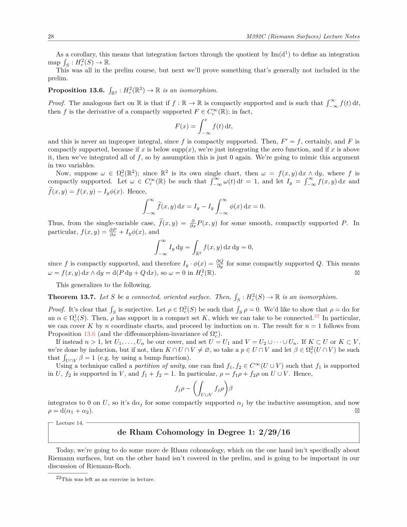
28 M392C (Riemann Surfaces) Lecture Notes
As a corollary, this means that integration factors through the quotient by Im(d1) to define an integrationmap
∫S
: H2c (S)→ R.
This was all in the prelim course, but next we’ll prove something that’s generally not included in theprelim.
Proposition 13.6.∫R2 : H2
c (R2)→ R is an isomorphism.
Proof. The analogous fact on R is that if f : R → R is compactly supported and is such that∫∞−∞ f(t) dt,
then f is the derivative of a compactly supported F ∈ C∞c (R); in fact,
F (x) =∫ x
−∞f(t) dt,
and this is never an improper integral, since f is compactly supported. Then, F ′ = f , certainly, and F iscompactly supported, because if x is below supp(x), we’re just integrating the zero function, and if x is aboveit, then we’ve integrated all of f , so by assumption this is just 0 again. We’re going to mimic this argumentin two variables.
Now, suppose ω ∈ Ω2c(R2); since R2 is its own single chart, then ω = f(x, y) dx ∧ dy, where f is
compactly supported. Let ω ∈ C∞c (R) be such that∫∞−∞ ω(t) dt = 1, and let Iy =
∫∞−∞ f(x, y) dx and
f(x, y) = f(x, y)− Iyφ(x). Hence,∫ ∞−∞
f(x, y) dx = Iy − Iy∫ ∞−∞
φ(x) dx = 0.
Thus, from the single-variable case, f(x, y) = ∂∂xP (x, y) for some smooth, compactly supported P . In
particular, f(x, y) = ∂P∂x + Iyφ(x), and∫ ∞
−∞Iy dy =
∫R2f(x, y) dxdy = 0,
since f is compactly supported, and therefore Iy · φ(x) = ∂Q∂y for some compactly supported Q. This means
ω = f(x, y) dx ∧ dy = d(P dy +Qdx), so ω = 0 in H2c (R).
This generalizes to the following.
Theorem 13.7. Let S be a connected, oriented surface. Then,∫S
: H2c (S)→ R is an isomorphism.
Proof. It’s clear that∫Sis surjective. Let ρ ∈ Ω2
c(S) be such that∫Sρ = 0. We’d like to show that ρ = dα for
an α ∈ Ω1c(S). Then, ρ has support in a compact set K, which we can take to be connected.22 In particular,
we can cover K by n coordinate charts, and proceed by induction on n. The result for n = 1 follows fromProposition 13.6 (and the diffeomorphism-invariance of Ω∗c).
If instead n > 1, let U1, . . . , Un be our cover, and set U = U1 and V = U2 ∪ · · · ∪ Un. If K ⊂ U or K ⊂ V ,we’re done by induction, but if not, then K ∩U ∩ V 6= ∅, so take a p ∈ U ∩ V and let β ∈ Ω2
c(U ∩ V ) be suchthat
∫U∩V β = 1 (e.g. by using a bump function).
Using a technique called a partition of unity, one can find f1, f2 ∈ C∞(U ∪ V ) such that f1 is supportedin U , f2 is supported in V , and f1 + f2 = 1. In particular, ρ = f1ρ+ f2ρ on U ∪ V . Hence,
fjρ−(∫
U∪Vfjρ
)β
integrates to 0 on U , so it’s dαj for some compactly supported αj by the inductive assumption, and nowρ = d(α1 + α2).
Lecture 14.
de Rham Cohomology in Degree 1: 2/29/16
Today, we’re going to do some more de Rham cohomology, which on the one hand isn’t specifically aboutRiemann surfaces, but on the other hand isn’t covered in the prelim, and is going to be important in ourdiscussion of Riemann-Roch.
22This was left as an exercise in lecture.

14 de Rham Cohomology in Degree 1: 2/29/16 29
Last time, we proved Theorem 13.7, that integration provides an isomorphism between H2c (S)→ R for all
smooth, oriented surfaces S. Today, we’re going to investigate H1(S): what does “closed 1-forms moduloexact 1-forms” mean? There are at least three or four answers, and we’ll go through two of them today.
Obstruction to Global Primitives. One answer is that it measures the obstruction to assembling localprimitives fi for a closed 1-form into a globally-defined primitive for α. Specifically, suppose S =
⋃i∈I Ui and
we know that α|Ui = afi; in this case, can we stitch these together into a global primitive? We’ll understandthis more precisely using Čech cohomology.
The answer begins with the following lemma.
Lemma 14.1 (Poincaré). H1(R2) = H2(R2) = 0.
In particular, a closed 1-form on a surface is locally exact. Thus, we can choose an open cover U of Ssuch that every U ∈ U is diffeomorphic to R2, and hence H1(U) = 0. Hence, if α ∈ Ω1(S) and dα = 0, thenα|Ui = afi, where fi ∈ Ω0(Ui). On the overlaps Uij = Ui ∩Uj , it’s not necessarily true that fi = fj . However,we do have d(fi − fj) = 0 on Uij , and hence cij = fi − fj is locally constant.
Definition 14.2.• A Čech 1-cochain ζ for (S,U) is an assignment of a locally constant ζij on Uij = Ui ∩ Uj for allUi, Uj ∈ U. These form a vector space, denoted C1(S;U) or C1.
• A Čech 1-cochain is a 1-cocycle if for all triples Ui, Uj , Uk ∈ U, the cocycle condition ζij + ζjk + ζki = 0on Ui ∩ Uj ∩ Uk. In particular, ζii = 0 and ζij + ζji = 0. 1-cocycles form a subspace Z1 ⊂ C1.
• A Čech 1-cocycle is a 1-coboundary if there exist locally constant functions fi ∈ Ω0(Ui) for eachUi ∈ U such that on Uij , ζij = fi − fj . The 1-coboundaries form a subspace B1 ⊂ Z1.
• Finally, we define the Čech cohomology H1(S;U) = Z1/B1.
The procedure above that assigned to a closed 1-form α the data (cij) defines a linear map c : H1(S)→H1(S;U), because (cij) is a cocycle, and is well-defined up to coboundaries. If α = df , we can takecij = f |Ui − fUj = 0.
Definition 14.3. A cover U of a surface S is acyclic if it’s locally finite and for all nonempty intersectionsUi1i2···iN = Ui1 ∩ · · · ∩ UiN , we have Hj(Ui1i2···iN ) = 0.
Hence, it suffices to make each intersection diffeomorphic to R2. Such an acyclic cover always exists: wecan embed S properly into RN for some N large, and then cover S by Euclidean balls in RN . By makingthem smaller if necessary (so S looks like a linear subspace).23
Theorem 14.4. If U is an acyclic cover, then c is an isomorphism.
Note. This is a special case of de Rham’s theorem; this formulation is due to André Weil. And as aninteresting corollary, this means the Čech cohomology is independent of the cover U, so long as it satisfies thehypotheses.
Proof of Theorem 14.4. Though we’ll write down an inverse map, let’s first see why c is injective. Supposec([α]) = 0, so that it’s a coboundary. Hence, α|Ui = afi and cij = fi−fj on Uij , and there exist locally constantfunctions ai ∈ Ω0(Ui) such that cij = ai − aj . Then, d(fi − ai) = α and (fi − ai)− (fj − aj) = cij − cij = 0on Uij , meaning there’s a g ∈ Ω0(S) such that g|Ui = fi − ai; hence, dg = α.
For surjectivity, let ρi be a partition of unity for U, so ρi ∈ Ω0(S), supp(ρi) ⊂ Ui, and∑ρi = 1. Now,
let ζ = (ζij) be any 1-cocycle. We do know there are smooth functions fi ∈ Ω0(Ui) such that fi − fj = ζij onUij . This is because the fi don’t have to be locally constant; in particular, we define
fi =∑Uj∈U
ρjζij .
23If you want to see this argument worked out in detail, search for the notion of a good cover, which is in between acyclicand having all intersections diffeomorphic to R2: a good cover is one for which all intersections are contractible.

30 M392C (Riemann Surfaces) Lecture Notes
A priori, this is only defined on Uij , since ζij is only defined there, but since ρj smoothly extends to 0 outsideUj , we can just define ρjζij to be 0 outside Uj . In any case, on Uij ,
fi − fj =∑k
ρk(ζik − ζjk)
=∑k
ρk(ζik + ζkj)
by the cocycle condition. Then, since all the ρk sum to 1,
=∑k
ρkζij = ζij .
Now, let αi = dfi, which is an exact 1-form on Ui, and αi − αj = d(fi − fj) = dζij = 0 on Uij , so the αi arerestrictions of a closed α ∈ H1(S), meaning ζij = c(α).
The injectivity of c is what we meant by thinking of H1 (the de Rham cohomology) as an obstruction tohaving a global primitive.
Dual to First Singular Homology. Another way of understanding H1(S) is as the dual to first singularhomology (with integral coefficients), i.e. H1(S) = HomAb(H1(S),R). That is, for any loop γ : S1 → S and aclosed 1-form α, we have the integral
I(γ, α) =∫S1γ∗α.
γ∗α is a closed 1-form on S1 ∼= R/Z, so it has the form f(t) dt for some f , and hence we can explicitlyintegrate.I is linear, and if α = dg is exact, then
I(γ,dg) =∫S1γ∗ dg =
∫S1
d(γ∗g) = 0
by the fundamental theorem of calculus. Thus, I(γ, α) depends only on the class of α in H1(S).Moreover, suppose we have a homotopy Γ : S1 × [0, 1]→ S between two loops γ0 and γ1. In this case,∫
S1γ∗0α−
∫S1γ∗1α =
∫S1×I
Γ∗(dα),
but since α is closed, then this is 0.24 In particular, I(γ, α) depends only on the free homotopy class of γ,which can be expressed as stating that I defines a bilinear map I : H1(S)×H1(S)→ R.25 In other words,we have a homomorphism of abelian groups H1(S)→ HomAb(H1(S),R) (i.e. to homomorphisms of abeliangroups), and since H1(S) is the abelianization of π1(S, ∗), this is also HomGrp(π1(S, ∗),R). (Here, ∗ is anypoint in S, regarded as the basepoint for the homotopy group.)
Theorem 14.5. The integration map I : H1(S)→ HomAb(H1(S),R) is an isomorphism.
This is another facet of de Rham’s theorem, in the form conjectured by H. Cartan, and also proved by deRham.
Proof idea. Let H1(S;R) denote Hom(H1(S),R), the first singular cohomology. The construction used inthe proof of Theorem 14.4 can be adapted to show that there’s an isomorphism H1(S;R)→ H1(S;U); then,one checks that the composition of that isomorphism with the one for de Rham cohomology is given by I.
24This calculation follows from Stokes’ theorem on surfaces, in case it seems confusing.25If the 1st homology group H1(S) isn’t intuitive to you, then think of it this way: if S is connected, H1(S) is the abelianization
of the fundamental group π1(S, ∗).

15 de Rham Cohomology in Degree 1: 2/29/16 31
Lecture 15.
Poincaré Duality: 3/2/16
Today, we’re going to finish our discussion of algebraic topology on surfaces by covering Poincaré duality,and then discuss what the complex structure does to vectors and covectors on Riemann surfaces.Theorem 15.1 (Poincaré duality). Let S be a connected, oriented smooth surface. Then, the bilinear map〈·, ·〉 : H1(S)×H1
c (S)→ R defined by〈[α], [β]〉 =
∫S
α ∧ β
is nondegenerate, so H1c (S) is dual to H1(S).
To prove this completely would be perhaps too much of a detour from our course, as we need to set upthe Mayer-Vietoris sequence for both H∗ and H∗c , and analyze what happens to the pairing under thesesequences. For a reference for the complete proof, see Bott and Tu’s book.
We will prove a weaker statement: that there is an injection ? : H1(S) → Hom(H1c (S),R) sending
[α] 7→ 〈[α], ·〉. In particular, when S is compact, the pairing is 〈·, ·〉 : H1(S) × H1(S) → R, and is skew-symmetric. Since it’s nondegnerate on one side, it’s therefore nondegenerate on the other, so the injectivityof ? implies it’s an isomorphism.
First, though, why is this pairing well-defined? Let’s compute it on an exact form dα and a closed form βwith compact support (so dβ = 0). Then,∫
S
dα ∧ β =∫S
d(α ∧ β) = 0,
by Stokes’ theorem. The analogous proof works for 〈α,dβ〉.
Proof. Suppose [α] 6= 0 in H1(S); we’d like to find a closed β ∈ Ω1c(S) such that
∫Sα ∧ β 6= 0.
Since α represents a nonzero class in cohomology, there must be a loop γ : R/Z→ S such that∫R/Z γ
∗α 6= 0.Without loss of generality, one can assume that γ is an embedding; there are several ways to argue this,e.g. homotope γ to a self-transverse immersion, thanks to the standard transversality theory package. Now,replace this immersed loop with one of its circle components (and the integral of α must be nonzero onat least one of them), so it’s now a piecewise smooth embedding, and then can be smoothed out with ahomotopy.
Now, given an embedded loop γ, we’ll construct a Thom form τγ , a closed 1-form supported in an annularneighborhood of γ such that for all closed 1-forms α on S,
(15.2)∫S
τγ ∧ α =∫R/Z
γ∗α.
That is, it will be a sort of dual to γ itself.First, let’s fix an annular neighborhood (that is, a tubular neighborhood) U for γ. This is a smooth
embedding of a cylinder Γ : (−1, 1)× S1 → S with the property that γ(0, t) = γ(t); let’s take Γ to preserveorientation. It suffices to construct τγ on (−1, 1) × S1, and then embed it in S. We want to control theintegral on the left side of (15.2), so we’d like to restrict τγ to be compactly supported.
Fix a smooth φ : (−1, 1)→ R such that• φ(s) = 1/2 for s sufficiently close to 1, and• φ(s) = −1/2 for s sufficiently close to −1.
The precise shape of φ won’t matter beyond this description.Now, we can define τ = φ∗ ds = φ′(s) ds. If α ∈ Ω1(C) is such that dα = 0, then we have an inclusion map
i : S1 → C sending t 7→ (0, t) and a projection map p : C → S1 sending (s, t) 7→ t; the homotopy invarianceof de Rham cohomology implies that α− p∗i∗α = df for some f ∈ C∞(C).
We can check that τγ is closed:
dτγ = ∂
∂tφ′(s) dt ∧ ds = 0,
so by Stokes’ theorem, since τγ is compactly supported,∫C
τγ ∧ df =∫C
d(τγ ∧ f) = 0.
32 M392C (Riemann Surfaces) Lecture Notes
In particular,∫Cτγ ∧ α =
∫Cτγ ∧ α′, where α′ = p∗i∗α, and we can compute this directly:∫
C
τγ ∧ α′ =∫∫
(−1,1)×S1
φ′(s)g(t) dsdt
=∫ 1
−1φ′(s) ds
∫S′g(t) dt
=∫S1i∗α =
∫S1γ∗α.
Poincaré duality generalizes to higher dimensions; the proof is harder, but the Thom form generalizes verynicely.
Corollary 15.3. If γ1 and γ2 are embedded loops in S, then∫Sτγ1 · τγ2 is the signed intersection number of
γ1 and γ2.
Proof sketch. The construction given in the previous proof doesn’t depend on the choice of tubular neighbor-hood, so let’s use this freedom to choose tubular neighborhoods such that the curves look “standard” nearintersection points, i.e. like coordinate axes (which entails making the curves transverse). If γ1 is travelingrightwards, assign +1 if γ2 is traveling up and −1 if it’s traveling down; then, it’s quick to check that thispoint contributes that value to
∫Sτγ1 ∧ τγ2 .
Note. Let Σg be a compact, oriented surface of genus g. In this case, H1(Σg) ∼= Z2g, spanned by loopsa1, . . . , ag, b1, . . . , bg, where ai goes around the ith hole and bj loops from that hole to the edge (if g = 1, aslice of the donut). In this case, the intersection form is ai · aj = 0, bj · bj = 0, and ai · bj = ∂ij .
Thus, by Poincaré duality, H1(Σg) ∼= R2g, with a basis αi = τai and βj = τbj . This is in fact a symplecticbasis with respect to 〈·, ·〉:
∫Σg αi ∧ αj = 0,
∫Σg βi ∧ βj = 0, and
∫Σg αi ∧ βj = −
∫Σg βj ∧ αi = 0.
Now, let’s specialize to Riemann surfaces. We’ll do a taste now, and then turn to elliptic curves; later on,we’ll need more and develop more. There is a smooth, even linear map i : C→ C that is multiplication by i.Its derivative j = D0i : T0C→ T0C is just i again, under the natural identification of T0C and C.
If X is a Riemann surface, it has a complex structure, consisting of a R-linear map Jx : TxX → TxX suchthat J2
x = −id for each x ∈ X and varying smoothly in x. This structure is just multiplication by i on thetangent space (the action of j) in holomorphic coordinates. This is independent of coordinates, because thechange-of-coordinates map is holomorphic, so its derivative is complex linear, and hence commutes with j.That is, a holomorphic atlas induces a smooth oriented atlas with a complex structure J .
One can also view J as a conformal structure; holomorphic maps C→ C with nonvanishing derivativesare conformal (infinitesimally preserving angles), thanks to the Cauchy-Riemann equations. This allowsus to measure the angle θ ∈ S1 between two nonzero tangent vectors e1, e2 ∈ TxX, where X is a Riemannsurface, because the holomorphic change-of-charts map will preserve it. In complex-structure terms, the anglebetween v and Jv is necessarily a right angle. That is, holomorphic maps with nonzero derivative are exactlythe angle-preserving maps. From this perspective, a complex structure is exactly the same as a conformalstructure, which is a way of measuring angles.
Another way to see this is that an oriented conformal structure on a smooth surface is the reduction ofthe structure group of its tangent bundle to SO(2)× R+, and a complex structure is the reduction of thestructure group to GL1(C) = C∗. In higher dimensions, the isomorphism of these groups no longer holds.
Lecture 16.
Holomorphic 1-Forms: 3/4/16
Today, we’ll discuss 1-forms on a Riemann surface, including holomorphic 1-forms on hyperelliptic Riemannsurfaces, corresponding to §5.3 and §6.1 in the textbook. This leads into calculating a distinguished,nonvanishing 1-form on certain Riemann surfaces, and to a discussion of elliptic curves.
Last time, we mentioned that a Riemann surface X comes with a complex structure J : TX → TX whichis rotation by 90 (multiplication by i) on each tangent space. In particular, above a point p ∈ X, Jp islinear, and J2
p = −id. We constructed it as the derivative of the map z 7→ iz in local coordinates.

16 Holomorphic 1-Forms: 3/4/16 33
There is an induced map J∗p on the cotangent space T ∗pX = Hom(TpX,R). Now, we can consider thecomplexified cotangent space (T ∗pX) ⊗ C, which is a two-dimensional complex vector space, and can bethought of as HomR(TpX,C). Since (J∗)2 = −id, we can decompose the complexified cotangent space intothe i- and −i-eigenspaces for J∗: T ∗pX ⊗C = T ∗pX
′ ⊕ T ∗pX ′′, where J∗ acts as +i on T ∗pX ′ and −i on T ∗pX ′′.Thus, T ∗pX ′ = HomC(TpX,C), the C-linear maps, and T ∗pX ′′ is the space of C-antilinear maps.
Similarly, we can decompose the complex-valued 1-forms (so letting p vary) Ω1(X)C = Ω1(X)⊗C∞(X,C)(the tensor is over C∞(X,R); Ω1(X) is a module over this ring). Hence, an α ∈ Ω1(X)C locally lookslike f dx + g dy, where f and g are C-valued smooth functions, so αp ∈ T ∗pX ⊗ C. Now, we apply thedecomposition into ±i-eigenspaces to get that Ω1(X)C = Ω1,0(X) ⊕ Ω0,1(X), where Ω1,0(X) is valued inT ∗pX
′ and Ω0,1(X) is valued in T ∗pX ′′. Explicitly, a complex-valued 1-form α splits as α = α1,0 + α0,1, whereif v is a tangent vector we have
α1,0(v) = 12(α(v)− iα(Jv))
α0,1(v) = 12(α(v) + iα(Jv)).
It’s quick to check that the first one is C-linear, the second is C-antilinear, and they sum to α(v).If we let dz = dx+ i dy and dz = dx− i dy, then a (1, 0)-form locally looks like f(x, y) dz and a (0, 1)-form
locally looks like g(x, y) dz. In particular, if f is a holomorphic function on X, then df ∈ Ω1,0(X): df = ∂f∂z dz,
because ∂∂z is 0 for any holomorphic function.
The exterior derivative also splits. Akin to the exterior derivative on real differential forms, we haveΩ0(X)C = C∞(X,C) and Ω2(X)C = Ω2(X)⊗ C∞(X,C). Then, d extends C-linearly, meaning our complexde Rham complex is the sequence
Ω0(X)Cd // Ω1(X)C
d // Ω2(X)C.
Now, when we split Ω1(X)C, each arrow also splits into two.
Ω1,0(X)∂
%%Ω0(X)C
∂
99
∂ %%
Ω2(X)C
Ω0,1(X)∂
99
For d : Ω0(X)C → Ω1(X)C, the splitting is d = ∂ + ∂, so for a smooth f , in local coordinates we have
df = ∂f + ∂f
= 12(fx − ify) dz + 1
2(fx + ify) dz
= ∂f
∂zdz + ∂f
∂zdz.
For d : Ω1(X)C → Ω2(X)C, we let ∂ = d|Ω1,0 and ∂ = d|Ω0,1 ; if Adz ∈ Ω0,1(X), then
∂(Adz) = ∂A
∂zdz ∧ dz = 2i∂A
∂zdx ∧ dy.
Correspondingly, if B dz ∈ Ω1,0, then
∂(B dz) = ∂B
∂zdz ∧ dz = −2i∂B
∂zdx ∧ dy.
With this C-linear algebra in mind, we have the following definition.
Definition 16.1. A holomorphic 1-form on X is an α ∈ Ω1,0(X) such that ∂α = 0.
34 M392C (Riemann Surfaces) Lecture Notes
That is, it’s closed and in Ω1,0. Such a form locally looks like α = A dz, where A is a holomorphic function.Using this, one can define the Laplacian ∆ : Ω0(X)→ Ω2(X), sending real functions to real 2-forms, given
by the formula∆ = 2i∂∂ = −2i∂∂.
In local coordinates, ∆f = −(fxx + fyy) dx ∧ dy.26
Definition 16.2. A smooth φ is harmonic if ∆φ = 0.
Lemma 16.3. If φ is harmonic, then locally, φ = Re(f), where f is holomorphic.
This is a classical theorem in complex analysis, albeit in a slightly different context.
Proof. You can prove this using the Poincaré lemma — suppose ∆φ = 0, and let A = 2 Re(i∂φ) = i∂φ+ i∂φ.Thus, dA = 2 Re(di∂φ) = 2 Re i(∂∂φ) = 0, since φ is harmonic.
Since A is closed, then it’s locally exact, so A = dψ for some real-valued function ψ. Hence, ∂ψ = A1,0 =−i∂φ and ∂ψ = A0,1 = i∂φ. Thus, ∂(φ+ iψ) = ∂φ+ i∂ψ = ∂φ− ∂φ = 0, so this function is holomorphic.
This ψ is sometimes called the harmonic conjugate of φ. The proof was really the same as the standardconstruction using the Cauchy-Riemann equations, though draped in different clothes.
From this, we immediately get the maximum principle.
Corollary 16.4 (Maximum principle). If a harmonic function φ has a local maximum near p, then it’sconstant near p.
Proof. Let φ = Re(f), for f holomorphic, and apply the open mapping theorem.
Again, this is the same proof as usual, just in a different guise.
Hyperelliptic surfaces.
Definition 16.5. A compact, connected Riemann surface Z is called hyperelliptic if there’s a degree-2 mapf : Z → S2.
Since a proper map is determined by its branching data, Z is identified with the Riemann surfaceX = (z, w) ∈ C2 | w2 = f(z), where the roots of f (the critical values) are all distinct (hence it really is aRiemann surface: repeated roots correspond to both partial derivatives vanishing). We haven’t looked at∞ yet, which will be important, but the reason this works is that f is a branched double cover for S2, andw2 = f(z) is a branched double cover, with the covering map projection onto z.
If C is a circle centered at the origin and large enough to contain all the roots of f in its interior, thenthe monodromy around C is the same as the composite of the monodromies around each root, since if weremoved the roots, the two loops would be homotopic. Hence, the monodromy is trivial if there are an evennumber of roots, and nontrivial if there’s an odd number, which allows us to understand the monodromy atinfinity. Let n be the number of roots.
In particular, if X∗ denotes the compactification of the algebraic curve X (i.e. the normalization of theprojective closure of X in CP 2), then if n is odd, then we just need to ad one branch point lying over ∞, andso X∗ = X ∪ P. If n is even, we need to add two points over ∞, and so it’s not a branch point.
Next time, we’ll construct a holomorphic 1-form α on X and see that it extends meromorphically toX∗; if n ≤ 4, this extension is holomorphic. This will lead to a discussion of Riemann surfaces that have anowhere-vanishing holomorphic one-form.
Lecture 17.
Hyperelliptic Riemann Surfaces: 3/7/16
Today, we’re going to discuss hyperelliptic Riemann surfaces and a special case of then, elliptic curves.This corresponds to §6.1 of the book.
Recall that a hyperelliptic surface is a compact, connected Riemann surface Z that admits a degree-2 mapF : Z → S2. Equivalently, there is a holomorphic action of the group Z/2 on Z, and Z/(Z/2) is biholomorphic
26This is the so-called “geometer’s Laplacian;” the “analyst’s Laplacian” has no minus sign. In Riemannian geometry, thischoice of the Laplacian is very natural.

17 Hyperelliptic Riemann Surfaces: 3/7/16 35
to S2 (which is nice because this is a branched double cover; the branched points are the fixed points of theaction).
One concrete realization of such a hyperelliptic surface is as the compactification X∗ of an algebraic curveX = (z, w) | w2 = f(z), where f has no repeated roots; then, the map F sends (z, w) 7→ z, so the criticalvalues are the roots of f , and possibly also ∞. Concretely, if n = deg(f) is odd, the X∗ = X ∪ P, and ifn is even, X∗ = X ∪ P1, P2: we know the inclusion X → CP 2 sending (z, w) 7→ [z : w : 1] extends to aholomorphic map X∗ → CP 2, so we just need to know what exists over [1 : 0] =∞. If n is odd, P ∈ crit(F ),and ∞ is a critical value; if n is even, them P± 6∈ critF , and ∞ isn’t a critical value. Hence, there’s alwaysan even number of critical values of F .
Topologically, imagine that you have a genus-g surface, and skewer it through its holes so that the skewerintersects the surface at 2g − 2 points. Then, rotating by 180 is a Z/2-action and these intersections arethe fixed points of that action. This is in fact that model for the Z/2-action on a hyperelliptic surface, andthe quotient is S2, but this is not easy to see. One way to think about it is to consider the map f : D→ Dsending z 7→ z2. If Z/2 acts on D by sending z 7→ −z, then f is Z/2-equivariant, and D = D/(Z/2). Then, ifwe excise a disc in the codomain, we have to remove two discs in the domain, as in Figure 7.
Figure 7. Visualizing the Z/2-action of a hyperelliptic surface.
Now, we can redraw this as a pair of pants mapping to the cylinder by a quotient, and the Z/2-actionbecomes rotating around the skewer in the middle. Now, if we stick several of these back-to-back, the moregeneral case of 2g − 2 branch points can be realized in this way, and capping off the cylinder gives you S2.
We’d like to relate these to holomorphic 1-forms, and the goal will be to show that if there are at most4 branch points, there exists a nowhere-vanishing holomorphic 1-form. Specifically, on X = (z, w) | w2 =f(z) ⊂ C2, the form α = dz/w is holomorphic for certain values of n.
A priori this looks meromorphic, rather than holomorphic, but on X, 2w dw = f ′(z) dz as complex 1-forms,so dz/w = z/f ′(z) dw. When w = 0, we know f(z) = 0, but therefore f ′(z) 6= 0 (since the roots of f aredistinct), and therefore there’s not actually a pole at w = 0.
To say that α is holomorphic is to say that ∂α = 0, i.e. locally, α = ϕ(z) dz, where ϕ is holomorphic. Thisis not a problem except maybe at ∞. If n is odd, then there is a holomorphic coordinate near P ∈ X∗ suchthat F takes the form F (τ) = τ2, given by τ2 = 1/z. Hence, we can directly substitute
f(z) = zn + a1zn−1 + · · ·+ an = τ−2n(1 + a1τ
2 + · · ·+ anτ2n)
and w = ±√f(z) = ±τ−n
√1 + a1τ2 + · · ·, and this square root is well-defined and holomorphic for τ in a
neighborhood of 0.The point is, α = dz/w, so
α = dzw
= τn√1 + α1τ2 + · · ·
(− 2τ3
)dτ
= −2τn−3√
1 + a1τ2 + · · ·dτ.
Hence, at P , where τ = 0:• α has a double pole if n = 1;• α is holomorphic and nonvanishing if n = 3; and• α has a 0 of order n− 3 if n > 3.

36 M392C (Riemann Surfaces) Lecture Notes
For n = 1, if you defined a “meromorphic 1-form” to be one that locally looks like a meromorphic function,then that’s what we get; for n = 3, the most interesting case, α is a holomorphic volume form on X∗, i.e. anowhere-vanishing holomorphic 1-form.
A similar analysis for n even shows that when n = 4, we once again get that α is a holomorphic volumeform.Note. Like regular volume forms, holomorphic volume forms are unique up to scaling: if Z is a compactRiemann surface and α1 and α2 are holomorphic volume forms, then there’s a c ∈ C∗ such that α2 = cα1;this is because α2 = fα1 for some holomorphic f : Z → C∗, but since Z is compact, then f must be constant(by the maximum modulus theorem).Elliptic Curves.Definition 17.1.
• An elliptic curve (E, p) is a compact, connected Riemann surface E together with a point p ∈ E suchthat E admits a holomorphic volume form.
• An isomorphism of elliptic curves f : (E1, p1)→ (E2, p2) is a biholomorphic map f : E1 → E2 thatmaps p1 7→ p2.27
Theorem 17.2. If E is a compact, connected Riemann surface and p ∈ E, then the following are equivalent.(1) (E, p) is an elliptic curve.(2) (E, p) ∼= (C/Λ, [0]) (meaning p is the equivalence class of 0) for a lattice Λ ⊂ C.(3) E embeds into CP 2 as a nonsingular Weierstrass cubic; that is, it’s the projective closure of an
equation w2 = (z − a1)(z − a2)(z − a3) for distinct a1, a2, a3, where p is the point at infinity.(4) There exists a branched cover F : E → S2 of degree 2 branched over exactly four points, where p is
one of the critical points.Remark.
• Condition (2) means that Aut(E), the biholomorphic maps E → E, acts transitively on E, and areinduced from translations of C. Hence, all choices of p are equally good.
• Nonetheless, the choice of p will be useful when we classify elliptic curves, and later, using theRiemann-Roch theorem, we’ll introduce a group law on an elliptic curve, and it will be helpful tohave p around.
• Later, there will be another equivalent condition, that E has genus 1 (so topologically a torus); rightnow, we can see that (2) implies this, and later will show that it implies (3).
We’ve proven (4) implies (1) by the discussion earlier this lecture, so our challenge is to run the rest of theproof. The idea for (1) implying (2) is that we need to construct a lattice given an elliptic curve; we’d liketo do this so that if q : C C/Λ is the projection map and β is the holomorphic 1-form on C/Λ such thatq∗β = dz, then we’d like the isomorphism F : E → C/Λ to set F ∗β = α.
If we knew H1(E) = Z2 = 〈a, b〉, we could do this more explicitly: let Λ be the period lattice of α, i.e. thepoints
Λ =∫
γ
α | γ is a 1-cycle in E.
Since a and b generate H1(E), this means Λ = Z∫aα+ Z
∫bα, so we really get a lattice; then, we can define
F : E → C/Λ by sending x 7→∫ xpα mod Λ (this is not well-defined, but does define a unique point in C/Λ).
Since we don’t yet know H1(E) = Z2 (even though a posteriori we will discover this), we will have to worka little harder to make an analogous construction.
Lecture 18.
Elliptic Curves and Elliptic Functions: 3/9/16
Today, we’re going to make some headway on Theorem 17.2; specifically, we’ll prove (1) implies (2), andthen prove that every elliptic curve embeds as a Weierstrass cubic into C2, which uses elliptic functions,which we’ll also discuss.
27This is not required to do anything special to the volume form; this means that the different scaled versions of a differentvolume give you isomorphic elliptic curves.

18 Elliptic Curves and Elliptic Functions: 3/9/16 37
Let (E, p) be an elliptic curve and α be a choice of holomorphic volume form. We have the abelian groupof periods
ΛE,α =∫
γ
α | γ is a 1-cycle in E.
This is a subgroup of C, and we can say a lot about this.
Theorem 18.1. With (E, p) and α as above,(1) ΛE,α is a lattice in C;(2) there is a unique biholomorphic map F : E → C/ΛE,α sending p 7→ [0] and such that F ∗(dz) = α;
and(3) if Λ1 and Λ2 are lattices in C and φ : C/Λ1 → C/Λ2 is a biholomorphic map such that φ∗[0] = [0],
then φ∗[z] = [cz], where c ∈ C∗ is such that c(Λ1) = Λ2.
Proving this inevitably involves working with some technical issues; the textbook tries to deal with theseminimally to avoid muddling the proof idea, but it’s not too hard to deal with them head-on.
Proof. First, we’ll attack (1). We must prove that Λ = ΛE,α is a lattice. We have a real, nowhere-vanishing1-form given by β = α + α; since α locally takes the form α = f(z) dz, then β locally takes the formβ = f dz + f dz (so their zeros would be the same).
The Poincaré-Hopf theorem28 states that the Euler characteristic is given by the number of times αvanishes, so χ(E) = 2− 2g = 0, and since 2g = dimH1(E), then g = 1, and H1(E;Z) = Z2 = Z · a⊕ Z · b.
Thus, Λ = Z∫aα+Z
∫bα. Thus, to show Λ is a lattice, it suffices to show that
∫aα and
∫bα are R-linearly
independent. So suppose they’re linearly dependent, so after rescaling α, Λ ⊂ R. Then, we can defineφ : E → R by φ(x) = Im
∫ xpα, which is independent of path. And φ is harmonic, because locally, it’s the
imaginary part of a holomorphic function, so by the maximum principle, φ is constant! Since φ(p) = 0,then φ = 0. However, dφ = Im(α), which by the open mapping theorem is not identically zero, which is acontradiction. Hence, Λ is a lattice, proving (1).
Next, for (2), define the period map or Albanese map F : E → C/Λ by
x 7−→∫ x
p
α mod Λ.
Clearly, F (p) = 0, and by construction, F ∗(dz) = α. Now, we would like to show that F is a biholomorphism.Since dF = α is nonvanishing, then F is locally biholomorphic. It’s also proper, because E is compact, andas such, it’s a covering map.
All finite coverings of C/Λ take the form C/L where L ⊂ Λ is a lattice, so (E, p) is identified with (C/L, [0]),and α is sent to dz, which is almost exactly what we wanted — but we don’t know that E is the period latticeyet. However, the period lattice of (C/L, dz) is exactly L, so the period lattice of E has to be L, i.e. L = Λ.
For (3), suppose we have such a φ. Then, φ∗(dz) = cdz for a c ∈ C∗, because these are the onlynonvanishing holomorphic 1-forms (so any two differ by a constant). In particular, φ′(z) = c and φ(0) = 0, soφ(z) = cz.
Now, we will talk about elliptic functions. The goal is to show that C/Λ is (biholomorphic to) the projectiveclosure in CP 2 of w2 = z3 + az + b ⊂ C2, where the cubic has distinct roots and the biholomorpism sends0 to the unique point at infinity.
Definition 18.2. An elliptic function for a lattice Λ ⊂ C is a meromorphic f on C with the property thatf(z + λ) = f(z) for all λ ∈ Λ and z ∈ C.
In other words, this function is translation-invariant by the lattice, so it descends to a meromorphicfunction on the quotient torus C/Λ.
Lemma 18.3. A holomorphic elliptic function is constant.
28We’ll discuss this theorem, and the Euler characteristic in general, in a few lectures; its proof does not depend on anythingwe do today.
38 M392C (Riemann Surfaces) Lecture Notes
This is by Liouville’s theorem (it’s defined just on the compact torus, and hence bounded and holomorphic);indeed, this is quite possibly why Liouville proved this theorem. Alternatively, you can use the fact that anyholomorphic function on a compact Riemann surface is constant, thanks to the maximum principle.
The most important elliptic function is the Weierstrass ℘-function.29
Definition 18.4. The Weierstrass ℘-function ℘ = ℘Λ is defined by
℘(z) = 1z2 +
∑λ∈Λ\0
(1
(z − λ)2 −1λ2
).
One also defines the Eisenstein seriesG2k(Λ) =
∑λ∈Λ\0
λ−2k.
We have a bunch of facts about these, which are somewhat straightforward estimates that are left asexercises. Alternatively, consult any text on elliptic functions.
Fact.• The series defining G2k converges absolutely for k > 1.• The series defining ℘ converges absolutely and uniformly on compact subsets of C/Λ, so ℘ is
meromorphic with double poles at each λ ∈ Λ, and is holomorphic on C \ Λ.• ℘ is an elliptic function for Λ.• ℘ is an even function: ℘(−z) = ℘(z).
The reason we care about ℘ is the following theorem.
Theorem 18.5. Any elliptic function for Λ is a rational function in ℘ and ℘′.
We can also write down the Laurent expansion for ℘ around z = 0. If |z| < |λ|, then
1(z − λ)2 −
1λ2 = 1
λ2
(1
(1− z/λ)2 − 1)
=∑n≥1
(n+ 1) zn
λn+2 .
Hence, if we take |z| ≤ min|λ| | λ ∈ Λ, then
℘(z) = 1z2 +
∑λ∈Λ\0
∑n≥1
(n+ 1) zn
λn+2
= 1z2 +
∑n≥1
((n+ 1)
∑λ∈Λ\0
λ−n−2
)zn.
Since ℘ is even, it only has even powers in its Laurent series, so
(18.6) ℘(z) = 1z2 +
∑n≥1
(2n+ 1)G2n+2(Λ)z2n.
Lecture 19.
The j-invariant and Moduli of Elliptic Curves: 3/11/16
“There are going to be some constants in this picture, and you’re going to think they lookstupid. But I promise you they’re not.”
29It’s so important that it gets its own typeface: it’s an old German p, but not the Gothic p! In LaTeX, you should use \wp totypeset ℘.

19 The j-invariant and Moduli of Elliptic Curves: 3/11/16 39
Today we’re going to finish the proof that C mod a lattice is a cubic curve, and then discuss the moduli spaceof elliptic curves and the j-invariant; this could be a whole subject, and makes contact with the world ofmodular forms.
Recall that last time, we took a lattice Λ ⊂ C and produced a Λ-invariant meromorphic function ℘ : C→ S2
(or C/Λ→ S2) defined by
℘(z) = 1z2 +
∑λ∈Λ\0
(1
(z − λ)2 −1λ2
).
We also calculated its Laurent series in (18.6) (recall that G2k(Λ) =∑λ λ−2k). We’ll now derive a differential
equation for ℘. From (18.6),
℘′(z) = − 2z3 +
∑n≥1
2n(2n+ 1)G2n+2z2n−1
= − 2z3 + 6G4z + 20G6z
3 +O(z5).
Therefore
(19.1) ℘′(z)2 = 4z6 −
24G4
z2 − 80G6 +O(z2).
Compare this to
℘(z) = 1z2 + 3G4z
2 + 5G6z4 +O(z6)(19.2)
℘(z)3 = 1z6 + 9G4
z2 + 15G4 +O(z6).(19.3)
What we would like to do is combine (19.1), (19.2), and (19.3) somehow in a way that eliminates all of theirpoles; since these are elliptic functions, such a combination would necessarily be constant, by Lemma 18.3.By inspection of the first few terms, we should take
℘′(z)2 − 4℘(z)3 + 60G4℘(z) + 140G4 = O(z2).The left-hand side is elliptic, holomorphic on C, and vanishes at 0, so it must be identically 0. Thus, if we letg2 = 60G4 and g3 = 140G6, ℘ satisfies the equation(19.4) (℘′)2 = 4℘3 − g2℘− g3.
All told, it really could have been worse; these estimates weren’t so bad.We’ll use this to map C/Λ to a cubic curve by the map θ : C/Λ→ CP 2 that sends [z] 7→ [℘(z) : ℘′(z) : 1]
(for z 6∈ Λ). Near z = 0, θ(z) = [z3℘(z) : z3℘′(z) : z3], and therefore approaches [0 : 1 : 0]. Hence, we letθ([0]) = [0 : 1 : 0]. This means that the image of θ is Im(θ) = X = y2z = 4x3 − g2xz
2 − g3z3 ⊂ CP 2.
Claim. The polynomial p(x) = 4x2 − g2x− g3 has three distinct roots, and hence X is a Riemann surfaceand the closure of y2 = p(x).
The last part does require smoothness at [0 : 1 : 0], but we’ve already checked that.
Proof. Returning to the differential equation (19.4), if 4℘(u)3 − g2℘(u)− ℘(u) = 0, then ℘′(u) = 0, whichseems like something we can work out. In fact, ℘′ is odd, so if λ ∈ (1/2)Λ, then ℘′(λ) = −℘′(−λ) = −℘′(λ),so it must be either 0 or ∞. We know (℘′)−1(∞) ∈ Λ, so all of the zeroes of ℘′ are in (1/2)Λ \ Λ, and in thefundamental domain there are three strict half-lattice points. In particular, if λ1 and λ2 are independentlattice vectors, the zeros of ℘′ are ℘(λ1/2), ℘(λ2/2), and ℘((λ1 + λ2)/2).
Are these still distinct after we’ve hit them with ℘? Yes, because ℘− ℘(λ1/2) is a degree-2, even functionwith a double zero at λ1/2< so it has no other zeroes. Thus, ℘(λ1/2) 6= ℘(λ2/2) and is also different from℘((λ1 + λ2)/2); the same argument works for λ2/2.
In particular, X is a Riemann surface. θ is non-constant, hence surjective by the open mapping theorem;since θ−1([0 : 1 : 0]) = [0], meaning it has multiplicity 1, then deg θ = 1, so it’s a biholomorphism. Thus,C/Λ ∼= X.
What does this to do an isomorphism f : C/Λ1 → C/Λ2? Last time, we saw this is of the form f([z]) = [cz],where c ∈ C∗ and cΛ1 = Λ2. Passing from Λ1 to Λ2 = cΛ1 is akin to rescaling the coefficients of the cubic:

40 M392C (Riemann Surfaces) Lecture Notes
g2(cΛ1) = c−4g2(Λ1) and g3(cΛ1) = c−6g3(Λ1), and so we get an isomorphism X1 → X2 by a change ofvariables x′ = c−2x and y′ = c−3y.
This concludes our proof of the equivalences of the various realizations of elliptic curves.
Classifying Elliptic Curves. We would like to set up and study a coarse30 moduli spaceM parameterizingelliptic curves up to isomorphism. The various models we have of elliptic curves all work to do this.
Let’s start with the Weierstrass cubic, for which an elliptic curve is represented as (the projective closureof) y2 = x3 + ax+ b. The right-hand side of this has distinct roots, so its discriminant δ is nonzero; if theroots are e1, e2, e3, then δ = (e1 − e2)2(e2 − e3)2(e3 − e1)2 = 4a3 + 27b2, which comes to us from Galoistheory.
First, let ∆ = −16δ. Then, our moduli space is M = (C2 \∆−1(0))/C∗, where C∗ acts by t · (a, b) =(t−4a, t−6b). Thus,M is in bijection with isomorphism classes of elliptic curves, by the preceding discussion.This is a one-dimensional complex manifold, or in other words, a Riemann surface!
Definition 19.5. Define the j-function (or j-invariant) j : M → C by j(y2 = x3 + ax + b) =−123a3/∆(a, b).
We can divide out by ∆(a, b) because it never vanishes. Thus, this is a pretty transparent construction ofthe j-invariant, if puzzling: why −1728?
Proposition 19.6. j is a biholomorphic map.
Well, that’s cool. Elliptic curves, up to isomorphism, are parameterized (coarsely) by C! We won’t provethis, but it’s a direct check of injectivity and surjectivity: you can use the C∗-action to work less hard.
But we can also express j in terms of lattices: if Λ is a lattice, C/Λ ∼= y2 = x3 − g2(Λ)x/4− g3(Λ)/4, soa3 = −g3
2/43 and ∆ = −16(−g32/42 + (27/4)g2
3). In particular, the j-invariant of the lattice Λ is
j(Λ) = 27(
g32
27g23 − g2
3
).
Any Λ can be rescaled to one of the form Λ = Z · 1 + Z · τ , where τ ∈ H; τ isn’t uniquely determined by Λ,but only up to the action of the modular group PSL2(Z) acting on H by Möbius maps. In other words, thislattice doesn’t have a unique Z-basis, but we can define J : H/(PSL2(Z))→ C by J([τ ]) = j(ΛZ·1⊕Z·τ ). Inparticular, H/PSL2(Z) is the space of lattices, and J is also biholomorphic. There’s a lot one could say aboutthis function as well: it’s invariant under τ 7→ τ + 1, and it has a Fourier expansion in powers of q = e2πiτ . Itturns out that this has the form
J(τ) = 1q
+ 744 +∑n≥1
cnqn,
where cn are positive integers that can be made explicit. On the one hand, this explains why we normalizedthe j-invariant we defined, but the 744?
Even more amazingly, Conway and Norton’s “monstrous moonshine“ conjecture (later a Fields Medal-winning proof) realizes these cn as dimensions of a graded algebra that the monster simple group actson!
Lecture 20.
The Euler Characteristic and the Riemann-Hurwitz Formula: 3/21/16
This week, we’re going to talk about the Euler characteristic, corresponding to Chapter 7 of the textbook.We’ll prove a bunch of interesting or cute facts, none of which are particularly deep; but after this, we moveinto the second part of the textbook, which has deeper results: Dolbeault cohomology, the Riemann-Rochtheorem, and the uniformization theorem.
30A coarse moduli space is one that does not keep track of automorphisms of a given object.

20 The Euler Characteristic and the Riemann-Hurwitz Formula: 3/21/16 41
The Riemann-Hurwitz Formula. To talk about the Euler characteristic we’ll need to exclude a fewpathological examples.
Definition 20.1. If S is a surface, it has finite (topological) type if dimHj(S) is finite for j = 0, 1, 2.
For example, all compact surfaces have finite type. A counterexample would be an infinite disjoint unionof spheres (for which H0 is infinite) or a surface with infinite genus (which has infinite-dimensional H1).
The Euler characteristic is an essentially topological definition.
Definition 20.2. If S is a surface of finite type, then its Euler characteristic is χ(S) = dimH0(S) −dimH1(S) + dimH2(S).
Proposition 20.3 (Mayer-Vietoris property). Suppose S = S0 ∪ S1 for open subsets S0, S1 ⊂ S. If S0, S1,and S0 ∩ S1 have finite type, then so does S, and χ(S) = χ(S0) + χ(S1)− χ(S0 ∩ S1).
The proof is immediate from the Mayer-Vietoris sequence for cohomology.31
The fact that singular cohomology with coefficients in R agrees with de Rham cohomology gives us thefollowing property, which is often taken as a more elementary definition of the Euler characteristic.
Proposition 20.4. If S is a surface with a finite triangulation, χ(S) is the number of vertices minus thenumber of edges plus the number of faces.
If f : S → T is a finite-degree covering map, one can pull a triangulation on T back to a triangulation onS; there are a number of different geometric or algebraic proofs of this, including one with spectral sequences!But the point is the following corollary.
Proposition 20.5. Let T be a surface of finite type and f : S → T is a degree-d covering map (d must befinite), then χ(S) = dχ(T ).
Now, we can state the Riemann-Hurwitz formula. Note, though, that there are typos in the textbook; theversion given in class is more accurate.
Theorem 20.6 (Riemann-Hurwitz formula). Let X and Y be compact Riemann surfaces and f : X → Y bea surjective holomorphic map that’s nowhere locally constant.32 Then,(20.7) − χ(X) = −deg(f)χ(Y ) +Rf ,
where Rf , the total ramification, is given by
(20.8) Rf =∑x∈X
(kx − 1),
where kx is the local multiplicity of f at x (i.e. there are coordinates centered at x in which f(z) = zkx).
The sum in (20.8) is finite because kx = 1 unless x is a critical point, and because X and Y are compact,there are only finitely many critical points. The theorem might be true for noncompact X and Y with certainproper maps f , but we’re only going to need it in the compact case.
The signs in the formula (20.7) are hard to remember, but if you can do the calculation below, you’ll befine.
Example 20.9. We know that if X is a genus-g hyperelliptic Riemann surface, then X is branched over bpoints in S2, where b = 2g + 2 (this was the “skewering” that we constructed a few lectures back). This is aconsequence of Theorem 20.6: χ(X) = 2− 2g, so −χ(X) = 2g − 2, and the right-hand side is 2(−2) + b (eachcritical point contributes 1 to the total ramification), and so 2g − 2 = b− 4, or b = 2g + 2.
Trying this with a genus-1 curve over the 2-sphere can help you remember the sign rule in a pinch.We’ll prove this momentarily; first, we present some corollaries.
Corollary 20.10. The total ramification Rf is even.
31Vietoris did work on this in the 1920s, but lived until 2002! He was Austria’s oldest citizen for some time, which is alsosurprising because the oldest citizen is usually a woman. How different the subject must have looked at the end of his life fromwhat he grew up studying!32If X and Y are connected, then all this means is that f is nonconstant.
42 M392C (Riemann Surfaces) Lecture Notes
This is because χ(X) and χ(Y ) are both even: a hyperelliptic surface can’t be branched at three pointsover the 2-sphere.
Corollary 20.11. Let X and Y be compact, connected Riemann surfaces and f : X → Y be a nonconstantholomorphic map. Then, the genus of X is at least the genus of Y .
For example, you can’t map S2 → T 2 (or any higher-genus surface) except by the constant map.
Proof. Let g(S) denote the genus of a surface S. If g(Y ) = 0, there’s nothing to prove, so suppose g(Y ) > 0,or −χ(Y ) ≥ 0, and therefore the right-hand side of (20.7) is −deg f · χ(Y ) +Rf ≥ −χ(Y ), because −deg fis nonnegative and Rf is nonnegative. Thus, 2g(X)− 2 ≥ 2g(Y )− 2.
This is interesting because it’s a restriction on what kinds of holomorphic maps can exist based on a purelytopological input. The converse is not true, however: there are Riemann surfaces of the same genus (e.g.different elliptic curves) with no nonconstant maps between them.
Proof of Theorem 20.6. Let ∆ ⊂ Y be the set of critical values; since Y is compact, this is finite, so letb = |∆|. Let N∆ be a small neighborhood of ∆ consisting of a small closed disc around each δ ∈ ∆.
Let Y0 = Y \ N∆ and X0 = f−1(Y0), so f : X0 → Y0 is a proper map with no critical points, hence acovering map of degree d = deg(f). Thus, by Proposition 20.5, χ(X0) = dχ(Y0). Now, we’ll relate χ(X) andχ(Y ) to this relation.
We can use the Mayer-Vietoris property, Proposition 20.3, to show that χ(Y ) = χ(Y0) + bχ(D)− bχ(A),where D is a disc and A is an annulus. Since D is contractible, χ(D) = 1, and since A ' S1, then χ(A) = 0.Thus, χ(Y ) = χ(Y0) + b.
Next, let’s look at X. Over each δ ∈ ∆, we’re gluing a number of discs to X0, where the fibers over pointsnear δ are grouped by monodromy cycles. Thus, for each critical point x ∈ f−1(δ), we’re gluing kx discs (e.g.if the monodromy is trivial, we glue in one disc), so the number of discs over preimages over δ is
d−∑
x∈f−1(δ)
(kx − 1).
Thus,
χ(X) = χ(X0) +∑δ∈∆
(d−
∑x∈f−1(δ)
(kx − 1))
= χ(X0) + db−∑
x∈crit(f)
(kx − 1).
Combining this with the formula for χ(Y ), we get that χ(X) +Rf = dχ(Y ).
The proof ultimately comes from the way we counted the discs that we’ve glued in.Here’s another nice application of the Riemann-Hurwitz formula.
Theorem 20.12. Let X be a compact, connected Riemann surface of genus g ≥ 2 and G be a finite group ofautomorphisms acting on X. Then, |G| ≤ 84(g − 1).
Remark.(1) It turns out that Aut(X) is also finite, so one can take G = Aut(X). This is a stronger theorem,
and doesn’t follow from the Riemann-Hurwitz theorem. The proof emerges from the Riemann-Rochformula; one has a finite set of points, called Weierstrass points permuted by Aut(X), and the inducedmap Aut(X)→ SN will be injective. Of course, the automorphism group of a genus-0 or 1 surfaceisn’t finite.
(2) Klein’s quartic curve X has genus g = 3 and |AutX| = 168 = 2 · 84, so this bound is satisfied.(Aut(X) is actually the simple group of order 168, PSL2(F7).) It’s known that the bound is sharp forsome infinite sequence of genera.
Proof of Theorem 20.12. It turns out that Y = X/G has the structure of a Riemann surface. This is notobvious, since points in X may have nontrivial stabilizers, but the proof is similar to that for Fuchsian groups.Near an x ∈ X with nontrivial stabilizer, find a G-invariant coordinate disc D, so that stabG(x) is a group ofautomorphisms of D fixing 0, and therefore a group of rotations. Thus, stabG(x) = µn: it’s the nth roots of

21 The Euler Characteristic and the Riemann-Hurwitz Formula: 3/21/16 43
unity for some n. That is, the projection X → Y is the map z 7→ zn, which we know gives the structure of asmooth manifold near x.
Now, let’s apply Riemann-Hurwitz to π : X → Y = X/G. The degree is |G|, so 2g(x)− 2 = |G|(2g(Y )−2) +Rπ. In the same way as the proof of the Riemann-Hurwitz formula, one can show (yes, this is an exercise)that
Rπ =∑
non-free orbitsy=G·x
(|G| − |stabG(x)|),
which therefore implies that2g(X)− 2|G|
= 2g(Y )− 2 +∑y
(1− 1|orbG(x)|
).
If g(X) ≥ 2, then the left-hand side of this equation is nonzero, so
(20.13) 2g(Y )− 2 +∑y=G·x
(1− 1|orbG(x)|
)> 0.
The somewhat magical fact is that if we minimize over g(Y ) ∈ Z≥0 and e1, . . . , eN ≥ 2, then the minimumpositive value of
(20.14) 2g − 2 +N∑i=1
(1− 1
ei
)is 42.33 This, together with (20.13), shows that
2g(X)− 2|G|
≥ 142 ,
which proves the theorem.So why 42? To minimize (20.14), we should definitely set g = 0. Let E =
∑Ni=1(1− 1/ei), which needs
to be greater than 2; since ei ≥ 2, then 1 > 1− 1/ei ≥ 1/2, so we need N > 2 to get anything interesting.If N ≥ 5, then E ≥ 5 · (1/2) = 2 + (1/2), so we don’t do better than 1/2. If N = 4, we can exceed 2 by1/2 + 1/2 + 1/2 + 2/3, so we can get 1/6. If N = 3, we can use 2/3 + 2/3 + 3/4, giving us 1/12, which is better.We can take e1 = 2, so e2, e3 ≥ 3, and if they’re both at least 4, we get E ≥ 1/2 + 3/4 + 4/5 = 1/20, which isanother lower bound. . . but we actually achieve the minimum with e1 = 2 and e2 = 3, so E = 1/2+2/3+6/7,giving us 2 + 1/42.
This is essentially an exercise in Hartshorne’s algebraic geometry textbook.
Lecture 21.
Modular Curves: 3/23/16
Today, we’re going to talk about modular curves, which are covered in §6.3.2 and §7.2.4 of the textbook.One beautiful aspect of Riemann surfaces is how many interesting and nontrivial things you can do withjust examples (e.g. elliptic curves, which we’re already briefly discussed). Modular curves are where modularforms live, and these are loved by number theorists and representation theorists; hopefully, we can return tothese.
We’ve already talked about the modular group Γ = PSL2(Z) = SL2(Z)/±1. This acts on the upperhalf-plane H by Möbius maps, so the modular group is a Fuchsian group; the quotient Y = H/Γ is theRiemann surface of lattice Λ ⊂ C up to homothety (i.e. Λ ∼ cΛ for all c ∈ C∗), where τ ∈ H 7→ Λτ = Z ·1⊕Z ·τ .This Y is an interesting space, because it is also the moduli space of elliptic curves up to isomorphism.Through this identification, we found that the j-invariant defines a biholomorphic map J : Y → C.
Today (and for part of Friday’s lecture), we’re going to do the following.• Establish a fundamental domain for Γ acting on H.
33It’s the answer to the Ultimate Question of Life, the Universe, and Everything!

44 M392C (Riemann Surfaces) Lecture Notes
• Talk about modular curves YN = H/ΓN , where ΓN is a principal congruence subgroup of Γ; these arethe elements that reduce mod N to the identity. We’ll also discuss their compactifications. Throughthe Riemann-Hurwitz formula (Theorem 20.6), we’ll calculate their genus.
We begin with two group-theoretic facts.
Fact.• If
S =[0 −11 0
]and T =
[1 10 1
],
then Γ is generated by S and T . Geometrically, if τ ∈ H, S(τ) = 1/τ , so S is inversion, andT (τ) = τ + 1, meaning T is translation to the right.34
• One can see that S2 = I and (ST )3 = I, and these are in fact all the relations: Γ = 〈S, T | S2 =(ST )3 = I〉.
Definition 21.1. A fundamental region for Γ acting on H is a set X such that every Γ-orbit intersects theclosure X, and no two points of X lie in the same Γ-orbit.
Since we have to use the closure, this is not the same as a fundamental domain.
Theorem 21.2. If Ω = z ∈ H | |z| > 1, |Re z| < 1/2, then Ω is a fundamental region for Γ acting on H.
See Figure 8. Geometrically, this makes sense: T marches to the right by 1, so T (Ω) and Ω are distinct,and every orbit intersects Ω, and S inverts, so the inverses of things in Ω are inside the unit circle. Thismeans that Y looks like Ω: the two points of Ω are i and ρ = eiπ/3, corresponding to the square latticeΛi ∈ Y , which is invariant under multiplication by i (rotation by 90), and the hexagonal lattice Λρ ∈ Y ,which is invariant under multiplication by ρ (which is rotation by 60).
Ω
1−1
Figure 8. A fundamental region for Γ acting on H, as in Theorem 21.2.
Proof of Theorem 21.2. Pick an A ∈ SL2(Z), so A =[a bc d
]. If c = 0, then ad = 1, so A =
[±1 b0 ±1
]; in
particular, in this case, A = ±Tm is a translation. Correspondingly, if A is a translation, then c = 0.In general, we can directly compute a useful formula: if τ ∈ H, then
(21.3) Im(A(τ)) = Im(τ)|cτ + d|2
.
Now, we’re going to march through a few lemmas. The overarching idea is that, within some Γ-orbit, we’dlike to find the point in Ω that maximizes Im(τ); we will also show that given any Γ-orbit, we do have somesuch point, and then we’re done.
Lemma 21.4. If τ ∈ Ω and c 6= 0, then Im(A(τ)) < Im(τ).
This is a quick check using (21.3).
Lemma 21.5. If τ,Aτ ∈ Ω, then A = ±I, so Aτ = τ .
Proof. If c 6= 0, then by Lemma 21.4, Im(Aτ) < Im(τ) = Im(A−1Aτ) < Im(Aτ), which is a contradiction.Hence, c = 0, so A = ±Tm is a translation. However, Tm(Ω)∩Ω = ∅ unless m = 0, so A = ±I as desired.
34For a reference, see T. Apostol, Modular Functions and Dirichlet Series in Number Theory.

22 Modular Curves: 3/23/16 45
We’ve now shown that no two points of Ω lie in the same Γ-orbit, which is half of the proof. But we stillneed to show that every Γ-orbit is represented.
Lemma 21.6. Suppose τ∗ maximizes Im(τ) within its Γ-orbit; then, |τ∗| ≥ 1.
Proof. If |τ | < 1, then Im(Sτ) = Im(−1/τ) = Im(τ)/|τ |2 > Im(τ).
So in this case, you’re almost in Ω — but might be in a translate of it.Fix a τ0 ∈ H and let h = hτ0 : Γ→ R send γ 7→ Im(γ · τ0).
Lemma 21.7. h is bounded above.
Proof. One could approach this with hyperbolic geometry, but it’s just as true if you prove it directly:Im(Aτ0) = Im(τ0)/|cτ0 + d|2 by (21.3). However, cτ0 + d is a nonzero point in the lattice Λτ0 , and thereforeit cannot be arbitrarily close to 0, and therefore its modulus is bounded.
One lemma remaining.
Lemma 21.8. h attains its maximum.
Proof. Take a sequence τn = γn · τ0 such that h(τ0)→ suph, which is finite by Lemma 21.7. Thus, Im(τn) isalso bounded above. Using translations Tm, we may assume |Re(τn)| ≤ 1/2, so τn ∈ [−1/2, 1/2]× [0, suph].This is compact, so there’s a convergent sequence τnj converging to some τ∗. We’d like this to lie inthe orbit of τ0, but this is not immediate: we do know that τ∗ ∈ Γ · τ0. However, Γ is a Fuchsian group,so its action on the upper half-plane is properly discontinuous. That means that every point p ∈ H has aneighborhood N in which N ∩ (Γ · p) = p: we can separate the points in an orbit. (This is something weproved, in Proposition 9.3.) Thus, τnj must be constant for large j, and in particular τ∗ ∈ Γ · τ0. Thus, τ∗maximizes h.
In conclusion, let τ∗ maximize h, and through translations, we may assume Re(τ∗) ≤ 1/2, and byLemma 21.6, |τ∗| ≥ 1. Thus, τ∗ ∈ Ω, so Ω intersects all Γ-orbits.
On Y = H/Γ, we have to identify the two left and right sides of Ω because of T , and the two sides of thearc on the bottom, thanks to S. This makes the Riemann surface structure on Y look a little strange: thesemicircle around i in Ω is actually promoted to a full cuircle through z 7→ z2. Similarly, the map z 7→ z3
makes a neighborhood of ρ into a disc neighborhood.Another consequence is that one can tile H by translations of Ω (as with any fundamental domain or
region).
Lecture 22.
Modular Curves for Principal Congruence Subgroups: 3/25/16
Last time, we proved Theorem 21.2, which characterized a fundamental region (almost, but not quite, afundamental domain) for the modular group Γ = PSL2(Z). This region Ω is the set of z ∈ H with |Re z| < 1/2and |z| > 1.
Today, we’re going to talk about the subgroups QN = PSL2(Z/N) for N = 1, 2, 3, . . .. It’s a standardfact in modular arithmetic that reducing mod N defines a map ϕN : Γ→ QN which is surjective! Then, letΓN = ker(ϕN ). We’ve previously studied Γp for p prime, as in Example 9.2, but the primality is actuallyirrelevant: the action of ΓN on H is free for N ≥ 2.
Define YN = H/ΓN , which carries a residual action by QN ; let πN denote the projection YN YN/QN ∼=H/Γ = Y (by the third isomorphism theorem, more or less). These YN are quotients by Fuchsian groups,hence Riemann surfaces; they will be our principal object of study today.Y parameterizes lattices Λ ⊂ C, but since we’ve quotiented by a smaller group, we also remember some
extra structure: YN parameterizes lattices along with something called a level N structure modulo homothety(where Λ ∼ cΛ as usual, and which does something sensible to level structures). Since C/Λ is an abeliangroup, we can let (C/Λ)[N ] denote its N -torsion subgroup.
Definition 22.1. A level N structure on a lattice Λ is an isomorphism (C/Λ)[N ] ∼= (Z/N)⊕ (Z/N); in otherwords, it’s a Z/N -basis for the N -torsion.

46 M392C (Riemann Surfaces) Lecture Notes
Figure 9. Tiling the upper-half plane with translations of Ω by the actions of S and T .Source: http://www.math.mcgill.ca/goren/ModularForms07-08/ModularForms.html.
Similarly, since Y is a moduli space for elliptic curves, YN should be too, and should carry some extrainformation, also called a level N structure. Using the abelian group structure of the elliptic curve, one couldalso frame the level N structure in terms of torsion subgroups, but we’ll give a different definition.
Definition 22.2. A level N structure on an elliptic curve E is an isomorphism H1(E;Z/N) ∼= (Z/N)⊕(Z/N).
The main reason we care about these things is that they’re the home of modular forms for these particularprincipal congruence subgroups; we’ll hopefully get to that by the end.
First, though, can we come up with a fundamental region for the action of ΓN on H? Since ΓN is smaller,we should get a larger region. Let q = qN = |QN |, and let g1, . . . , gq ∈ Γ be representatives for the cosets ofΓN . Then, let ΩN be the interior of g1Ω ∪ · · · ∪ gqΩ; this is a fundamental region for ΓN . Depending on therepresentatives of cosets you picked, this might not be connected.
One corollary of this is that the projection map πN : YN → Y is proper; the preimage of a compact set iscontained in finitely many giΩ, and hence is still closed and bounded in H, hence compact.
Example 22.3. Let’s see what happens when n = 2. Then, the first column of a matrix in PSL2(Z/2) canbe anything except all zeroes, and the second column has the same, but can’t be a multiple of the first; thus,this gives us (4 − 1)(4 − 2) = 6 elements. We identify them up to multiplication in (Z/2)×, but this justcontains the identity; hence, we get 6 elements in PSL2(Z/2).
Let S and T be the generators we defined last lecture; then, we will take the cosets of Γ2 to be those givenby 1, T−1, S, T−1S, STS, and ST . We choose these because they produce a nice connected region of H,bounded by a hyperbolic hexagon. This includes a point at infinity, a “end” of Ω2. If ρ = eiπ/3, then onecan check that ST (ρ2) = ρ2, so ST is a rotation of order 3 around ρ2 (the center of the hexagon). Thesegive us the three “ends at infinity,” either going to infinity in the imaginary direction or touching the x-axis.T 2 ∈ Γ2, and it identifies the two vertical boundaries going to infinity.
The point is that Y2 is this hexagon with three pairs of adjacent edges identified. Making these identificationspinches them off, and so Y2 is biholomorphic to the thrice-punctured sphere, and π2 : Y2 Y is a degree-6map branched over two critical points, ρ and i (since these are the two non-free Γ-orbits); for these points,the stabilizers have size 3 and 2, respectively.
This example should aid visualization (the pictures were drawn on the blackboard; I couldn’t reproducethem quickly, but I encourage you to draw them, or look up a program that generates such fundamentaldomains).

23 Modular Curves for Principal Congruence Subgroups: 3/25/16 47
So for Y2, we can compactify it by putting in the three points at infinity, to obtain S2. In general, we cancompactify YN ; we’ll call the compactification XN .
• First, compactify Y to get S2, by adding a point at ∞.• Using the monodromy at ∞ for πN , we get a recipe for extending πN : YN → Y to a branched
covering πn : XN → S2; this is analogous to the construction we used in things such as the Riemannexistence theorem earlier in the course. Thus, XN is YN along with a number of “cusps” over∞ ∈ S2.
QN still acts on XN , where the cusps form exactly one QN -orbit; for N = 2, there are 3 cusps, and π2 hasbranching order 2 at each cusp.
We’re going to use the Riemann-Hurwitz formula (Theorem 20.6) to compute the genus g(XN ), thuscharacterizing YN as a surface of a specified genus minus a known number of points. To do this, we’ll defineΩN by taking the set of cosets I, T, T 2, . . . , Tn−1, and some others (many others, though we won’t writethem down). Thus, ΩN consists of a bunch of translates of Ω by T , plus some extra stuff given by the actionof S. The action of TN identifies the ends of P = Ω ∪ TΩ ∪ · · · ∪ Tn−1Ω, which wraps the ends to a cylinder,giving one cusp at infinity, but doesn’t affect whatever is going on with S. And in particular, it contains theneighborhood of exactly one cusp, and at this cusp, πN is branched to order N (around this cusp, it lookslike the cyclic map z 7→ zN ).
In general, for a finite group action G on a compact Riemann surface X, the proof of Theorem 20.12implies that
(22.4) − χ(X) = |G|(−χ(X/G) +
∑orbits
(1− 1|stabG x|
)).
For QN acting on XN , the nonfree orbits are those of ρ, whose stabilizer has size 3; i, whose stabilizer hassize 2; and ∞, whose stabilizer has size N . Plugging this into (22.4),
2g(XN )− 2 = qn
(−2 +
(1− 1
3
)+(
1− 12
)+(
1− 1N
))= qN
(16 − 1N
)= qN (N − 6)
6N .
That is, we’ve derived the following genus formula.
Proposition 22.5. With XN as in the above discussion,
g(XN ) = 1 + qN (N − 6)12N ,
where qN = |PSL2(Z/N)|.
Let’s make this more explicit: if N = p is an odd prime, |GL2(Z/p)| = (p2 − 1)(p2 − p) (since the firstcolumn can be anything nonzero, and the second column can be anything other than a multiple of the first),and the kernel of the quotient GL2(Z/p)→ (Z/p)∗ is SL2(Z/p), so we’ve divided by |(Z/p)∗| = p− 1, andtherefore |SL2(Z/p)| = p(p2 − 1). Thus, |Qp| = |PSL2(Z/p)| = p(p2 − 1)/2 for an odd prime p. That is,g(Xp) = (1/24)(p+ 2)(p− 3)(p− 5).
(1) By Example 22.3, g(X2) = 0.(2) g(X3) = 0 and g(X5) = 0, and 2, 3, and 5 are the only examples with genus 0.(3) g(X7) = 3. q3 = |PSL2(Z/7)| = 168. This is a famous example: PSL2(Z/7) is a nonabelian simple
group of order 168, and its action on X7 realizes the bound we found in Theorem 20.12: it has thelargest possible symmetry group.
These XN are where modular forms live; but that’s a story for another day.
Lecture 23.
Euler Characteristics and Meromorphic 1-Forms: 3/28/16
Today, we’re going to talk about the Poincaré-Hopf theorem.Let S be a compact, oriented surface and α ∈ Ω1(S) be a 1-form whose zeros are isolated. If p is a zero
of α, we’d like to assign it a multiplicity mα(p) ∈ Z, which we do as follows. Suppose (x, y) are orientedcoordinates centered at p, so that in these coordinates, α = α1 dx+ α2 dy. If γ is a small circle around p, so

48 M392C (Riemann Surfaces) Lecture Notes
that γ(t) = (r cos(2πt), r sin(2πt)), for t ∈ [0, 1], then α γ : R/Z→ R2 \ (0, 0); then, we defined mα(p) tobe the winding number of α γ. It’s easy to show this is independent of the coordinates we chose.
Theorem 23.1 (Poincaré-Hopf theorem for surfaces).
χ(S) = −∑
p:α(p)=0
mα(p).
There’s a more general version for manifolds; moreover, there’s a version that uses vector fields insteadof 1-forms, in which case the minus sign disappears. This can be found in many textbooks on differentialtopology (though, curiously, not Guillemin and Pollack’s); the proof generally involves relating both sides tothe self-intersection number of the diagonal ∆S ⊂ S × S, which is equal to the Euler characteristic (this is atheorem, since we didn’t define the Euler characteristic in this way).
Assuming Theorem 23.1, we derive the following corollary.
Proposition 23.2. Let X be a compact Riemann surface and θ be a holomorphic 1-form on X. Assumeθ isn’t identically 0 on any connected component of X (which automatically implies its zeros are isolated).Then,
χ(X) = −∑
p: θ(p)=0
kp(θ),
where in local coordinates, θ = f(z) dz, so we define kp(θ) to be the order of vanishing of f at p.
Proof. Let α = Re(θ) = (1/2)(θ + θ), so the zeros of α are the zeros of θ. Near such a zero, z = x+ yi, so ifθ = f(z) dz, then α = (Re f) dx+ (Im f) dy, and so the winding number of (Re f, Im f) around z = reiϑ isthe order of vanishing of f at 0, by Theorem 23.1.
Corollary 23.3. S2 has no nonzero holomorphic 1-forms.
This is because χ(S2) = 2, so∑kp(θ) ≤ 0 for any such θ.
We can also define kp(θ) when p is a pole of a meromorphic 1-form: if θ = f(z) dz and f has a pole oforder n at p, then we set kp(θ) = −n. For example, a simple pole contributes −1 to the sum.
Theorem 23.4. Let X be a compact Riemann surface and θ be a meromorphic 1-form on X that isn’tidentically 0 on any connected component of X. Then,
χ(X) = −∑
p: poles and zeroskp(θ).
This is the version of the Poincaré-Hopf theorem that we will find the most useful.
Proof. We know what happens at zeros of θ, so fix a coordinate disc Dp around each pole p. By shrinkingDp if needed, we can assume that the Dps are disjoint, and that θ doesn’t vanish on any Dp. Thus, each Dp
is biholomorphic to the closed unit disc D.We’d like to obtain an ordinary 1-form out of θ, but thanks to the poles this will be a little harder. Let
ψ : [0,∞)→ [0,∞) be a smooth function defined such that:• If 0 ≤ t ≤ 1, ψ(t) = 1.• If t ≥ 2, then ψ(t) = 1/t.• On (1, 2), ψ smoothly interpolates between these two curves.
Now, for a pole p, regarding Dp as D, we can write θ(z) = cf(z) dz, where c ∈ C× and f are chosen suchthat |f | ≤ 1 on the annulus z | 1/2 ≤ z ≤ 1.
Now, on Dp, set θp(z) = ψ(|f(z)|2)cf(z) dz. For 1/2 ≤ |z| ≤ 1, θp(z) = θ(z), so we can extend to a 1-formθ, which is defined to be θ outside of all Dp, and to be θp on Dp. This is a smooth 1-form (and has no poles),but isn’t holomorphic! Near p = 0 ∈ Dp, θp(z) = cf(z)/|f(z)|2 dz = c/f(z) dz, and therefore θp(0) = 0.
Thus, θ is a complex 1-form, whose zeros are the zeros and poles of θ, and so we can repeat the argumentthat proved Proposition 23.2, checking that the multiplicities for α = Re(θ) are exactly the values of kp(θ);the trick with the poles is that the complex conjugate we had in a neighborhood of p switches the sign to thecorrect one.

24 Euler Characteristics and Meromorphic 1-Forms: 3/28/16 49
There might be ways to prove this that lie entirely within algebraic geometry.One consequence of Theorem 23.4 is that it allows a new proof of the Riemann-Hurwitz formula, Theo-
rem 20.6. Recall that this says if X and Y are compact Riemann surfaces and f : X → Y is smooth, then−χ(X) = −(deg f)χ(Y ) +Rf , where Rf is the total ramification of f , defined in (20.8).
Proof of Theorem 20.6 using Theorem 23.4. This proof is contingent on the existence of a nonvanishing,meromorphic 1-form θ on Y ; this exists by the Riemann-Roch theorem, which we will prove later. Thus, f∗θis a meromorphic 1-form on X; we’d like to apply our formula to it.
Let p ∈ X be a pole of f∗θ. Let z be a holomorphic local coordinate for X centered at p, and wbe a holomorphic local coordinate for Y centered at f(p). We can (and do) choose z and w such thatf(z) = w = zm, where k is the multiplicity of f at p.
In w-coordinates, θ = g(w) dw, so f∗θ = g(zk) d(zm) = mg(zm)zm−1 dz; hence, if mf(p)(θ) = `, then f∗θhas multiplicity m`+m− 1 at f(p).
For x ∈ X, let mx denote the multiplicity of f at x, and for all y ∈ Y , let `y = kθ(y). Thus,∑x∈f−1(y)
kf∗θ(x) =∑
x∈f−1(y)
(mx`y +mx − 1)
= (deg f)`y +∑
x∈f−1(y)
(mx − 1).
Summing over y ∈ Y , we get that
−χ(X) = −(deg f)χ(X) +∑x∈X
(mx − 1).︸ ︷︷ ︸Rf
This is useful for generalizing the Riemann-Hurwitz formula to branched coverings of higher-dimensionalcomplex manifolds.
Another useful consequence of Theorem 23.4 is to calculate the genus of plane algebraic curves.
Theorem 23.5. Let P be a degree-d homogeneous polynomial in C[z0, z1, z2] and X = P = 0 ⊂ CP 2.Suppose that the ∂P
∂zidon’t all vanish at any point, so X is a Riemann surface. Then, the genus of X is
g(X) = 12(d− 1)(d− 2).
This is quite powerful for characterizing genera of algebraic curves: a degree-1 or 2 curve must have genus0, a cubic must be degree 1, and in general we only get triangular numbers.35
Proof. Fix a projective line L ⊂ CP 2 which intersects X at d distinct points; this is a generic condition,so we can always find such an L. We can make a change of coordinates of CP 2 such that L is the line at∞, the points of the form [0 : z1 : z2]. Thus, on CP 2 \ L, we have coordinates (z, w) = (Z1/Z0, Z2/Z0); setp(z, w) = P (1, z, w). On X, this means that
dp = ∂p
∂zdz + ∂p
∂wdw = 0,
so if we let
θ = dz∂p/∂w
= − dw∂p/∂z
,
then this is a holomorphic, nowhere-vanishing 1-form on X. Then, computing the multiplicities of the zerosof θ calculates χ(X) and therefore also g(X) (see the textbook for more details).
35This is a special case of a adjunction formula characterizing the genus of a compact Riemann surface embedded in moregeneral manifolds, and which admits an entirely topological proof.

50 M392C (Riemann Surfaces) Lecture Notes
Lecture 24.
The Riemann-Roch Theorem: Background and Statement: 3/30/16
“For a while, everything is going to be formal, until it won’t be.”Today, we’re going to start part III of the textbook, which centers on the Riemann-Roch theorem, which isreally the most fundamental theorem of compact Riemann surfaces. (Uniformization would be the fundamentaltheorem for noncompact surfaces.)
Today, we’ll discuss the background, and over the next two lectures, we’ll discuss some applications. Afterthat, we’ll provide the proof, which begins geometrically and ends with the very analytic story of inverting aLaplacian.
For the rest of this lecture, X will denote a Riemann surface.
Divisors on a Riemann surface. Let MX denote the field of meromorphic functions X → S2 andM×X =MX \ 0. For any x ∈ X, we can define a valuation vx :M×X → Z as follows: in a local coordinate zcentered at x, write f ∈M×X as its Laurent series: f(z) = czm +O(zm+1). Then, we define vx(f) = m.
Here are some basic properties of this valuation.• vx(f) ≥ 0 iff f is holomorphic near x, and vx(f) > 0 iff f is holomorphic near x and f(x) = 0.• If f, g ∈M×X , vx(fg) = vx(f) + vx(g) and vx(f + g) ≥ min(vx(f), vx(g)).
It may seem a bit curious to make this anM×X -valued function, rather than an X-valued function, but thesenice properties are why we do this; some divisors arise when we think of this as an X-valued function, though.
Definition 24.1. A divisor on X is a function D : X → Z sending x 7→ Dx with finite support.
That is, Dx = 0 for all but finitely many x. A divisor is often written as the sum
D =∑x∈X
ax · x,
where ax = Dx ∈ Z. Since Z is an abelian group, one can add divisors pointwise to get an abelian groupDiv(X). Given a p ∈ X, one example of a divisor is the one D = p, whose value at p is 1 and whose valueseverywhere else is 0.
Now, assume X is compact. Then, any nonzero meromorphic function f ∈M×X defines a divisor
(f) =∑x∈X
vx(f) · x,
or vx(f) regarded as a function of x.
Definition 24.2. If D = (f) for some f ∈M×X , then D is a principal divisor.
The properties of vx imply that (fg) = (f) + (g) and (1/f) = (−f); hence, the principal divisors form asubgroup PDiv(X) ≤ Div(X). We’ll soon see that not every divisor is principal.
Definition 24.3. Two divisors D1 and D2 are linearly equivalent if D1 −D2 ∈ PDiv(X).
That is, they differ by the principal divisor associated to a nonzero meromorphic function. The group oflinear equivalence classes is called the class group C`(X) = Div(X)/PDiv(X).36
Definition 24.4. A divisor D is effective if its coefficients are all nonnegative; this is denoted D ≥ 0. Wewrite D1 ≥ D2 if D1 −D2 ≥ 0, which defines a partial order on DivX.
This partial order does not pass through to C`(X).
Definition 24.5. The degree of a divisor D =∑ax · x is
degD =∑x∈X
ax ∈ Z.
Thus, deg : DivX → Z is a homomorphism of groups.
Lemma 24.6. If D ∈ PDiv(X), then degD = 0.36A fact which we will not use: there is an isomorphism C`(X) ∼= Pic(X), where the latter is the Picard group of X.

24 The Riemann-Roch Theorem: Background and Statement: 3/30/16 51
Proof. It may come as no surprise that we’ll use the argument principle, (4.8). Choose an f ∈ M×X ; thus,deg((f)) = 0 is equivalent to the number of poles and zeros of f , counted with multiplicity, being equal.
Choose disjoint closed discs ∆1, . . . ,∆n, each containing a unique zero or pole of f . By the argumentprinciple,
deg((f)) =N∑i=1
∫∂∆i
dff.
Let X0 be X minus the interiors of all these discs, so X0 is a compact surface with boundary. Then, byStokes’ theorem,
N∑i=1
∫∂∆i
dff
= −∫∂X0
dff
= −∫X0
d(
dff
),
because df/f is nonsingular on X0. However, since f is holomorphic on X0, then d(df/f) = 0: in localcoordinates, df = f ′(z) dz, and so the only interesting thing can come from dz, but applying this to aholomorphic function gives you 0. Thus, deg((f)) = 0.
The point is that we can use Stokes’ theorem to bring the argument principle to general Riemann surfaces.37
As a consequence, we get a degree homomorphism deg : C`(X)→ Z.
Definition 24.7. Let D be a divisor; then, we will let OX(D) denote the sheaf of effective divisors, the sheafof functions defined as follows: if U ⊂ X is open, then OX(D)(U) is the set of f : X → S2 meromorphic onU and such that deg((f)) ≥ 0 on U .
These are the “functions with poles at worst D,” meaning that if D =∑axx is effective, f is allowed to
have poles only on suppD, and the order of the allowed poles at x is bounded by ax.The key definition is this one, whose notation is motivated by sheaf cohomology.
Definition 24.8. Let H0(OX(D)) = OX(D)(X) = f ∈MX | f = 0 or f ∈M×X and deg((f)) ≥ 0. Thiswill sometimes be abbreviated H0(D).
For example, if P and Q are distinct divisors on X, then H0(2P −Q) is the space of meromorphic functionswith at worst a double pole at P , and vanishing at Q.
In particular, H0(D) is a vector space, and if g ∈M×X , H0(D) ∼= H0(D + (g)) through the map f 7→ f/g.We will let h0(D) = dimH0(D), so that we have a function h0 : C`(X)→ Z≥0.
The Riemann-Roch problem is to compute h0(D). It’s worth putting this in context: a priori, for a generalcompact Riemann surface X, we don’t know if there are any nonconstant meromorphic functions!
We can make a few observations quickly, though.(1) If degD < 0, then H0(D) = 0, because if D + (f) ≥ 0, then deg(D + (f)) ≥ 0, but this was degD,
which is a contradiction.(2) IfD1 ≤ D2, thenD2 = D1+E, where E is an effective divisor. In this case, we haveH0(D1) ⊂ H0(D2):
if D = D′ + mp, where p 6∈ supp(D′), then choose f, g ∈ H0(D + p) = H0(D′ + (m + 1)p). Then,some linear combination af + bg has valuation at most m at p (intuitively, we’re canceling out largemultiple poles), i.e. af + bf ∈ H0(D). Thus, dim(H0(D + p)/H0(D)) ≤ 1, and we can repeat thisargument for the rest of supp(D) \ supp(D′).
(3) Combining these two, if D is linearly equivalent to an effective divisor, h0(D) ≤ degD + 1, since h0
is invariant under linear equivalence.On the other hand, D is linearly equivalent to an effective divisor iff H0(D) 6= 0, so in general our upperbound is
h0(D) ≤ max(0,deg(D) + 1).We still haven’t said anything that implies there are nontrivial meromorphic functions on X yet. That’swhere the Riemann-Roch inequality comes in.
Theorem 24.9 (Riemann-Roch inequality38). If X is a compact, connected Riemann surface and D is adivisor on X, then h0(D) ≥ degD + 1− g(X).
37A related theorem which is distinct, but has a very similar proof, is the residue theorem for compact Riemann surfaces, whichshows that the sum of the residues and orders of zeros of a meromorphic function on a compact Riemann surface is 0.38This is also called the weak Riemann-Roch theorem.

52 M392C (Riemann Surfaces) Lecture Notes
The proof of this will have to wait.
Corollary 24.10. Every compact Riemann surface admits nonconstant meromorphic functions.
Proof. It suffices to prove this on a connected component of a compact Riemann surface X, so we can useTheorem 24.9. Let D be effective of degree D, so h0(D) ≥ degD + 1− g(X) > 1, so H0(D) contains morethan just constant functions.
Of course, the Riemann-Roch inequality is a more precise result than this, but it’s still a nice fact to know.
Corollary 24.11. If X is a compact, connected Riemann surface and g(X) = 0, then X is biholomorphic toS2.
Before this, all we knew was that X is diffeomorphic to S2.
Proof. Take a p ∈ X, and regard it as a divisor. Then, h0(P ) ≥ 1 + 1 − 0 = 2, so there is a nonconstantf ∈ H0(p), which has a single, simple pole. In particular, f : X → S2 has exactly one pole, so it’s a degree-1map, and therefore is biholomorphic.
There’s also a strong (or full) Riemann-Roch theorem, which measures the discrepancy between h0(D)and degD + 1− g(X).
Definition 24.12. Let H0(KX(D)) denote the vector space of meromorphic 1-forms on X with poles atworst D.
This is defined in local coordinates: if α is a meromorphic 1-form, then in local coordinates z, α = f(z) dz,and we require that vf (x) ≤ m (meaning zmf(z) is holomorphic).
Theorem 24.13 (Riemann-Roch). Let D be a divisor on the compact Riemann surface X. Then,dimH0(OX(D))− dimH0(KX(−D)) = degD + 1− g.
This means that we’re comparing the dimensions of the meromorphic functions with poles at worst D andmeromorphic 1-forms with zeros at worst D.
Lecture 25.
: 4/1/16
Lecture 26.
Modular Forms: 4/4/16
“We’re not going to prove Fermat’s last theorem today; maybe next week.”Last time, we discussed some applications of the Riemann-Roch theorem motivated towards algebraic geometry,e.g. embedding surfaces in projective space.
Today, we’re going to discuss modular forms, a related but different application. There are many referencesfor this material:
• Diamond and Shurman, A First Course in Modular Forms, though they seem to make a meal of it.39
• Of course, Serre’s A Course in Arithmetic is beautiful.• Milne’s online modular forms course notes are also a great reference.
Modular forms touch on a great deal of current research in representation theory and number theory, mostfamously in the modularity theorem of Wiles et. al., which led to the proof of Fermat’s last theorem. Buttoday, we’re going to do some basics.
Throughout today, let Γ = PSL2(Z), the modular group, and ΓN be the kernel of the reduction modN , Γ → PSL2(Z/N) (so Γ1 = Γ). Thus, ΓN acts on the upper half-plane H, and YN = H/ΓN . Thecompactification XN = YN ∪ cusps, which are a single orbit of ΓN . The number of cusps is |ΓN |/N .Through the j-invariant, we proved that Y1 = H/Γ1 ∼= C, and X1 ⊃ Y1 is biholomorphic to S2 = C ∪ ∞:there’s one cusp.
Modular forms are special examples of weakly modular functions.
39If you, like me, didn’t recognize this colloquialism, it means “to make a [slight] mess of it.”

26 Modular Forms: 4/4/16 53
Definition 26.1. Let k ∈ Z. A weakly modular function of weight 2k for the group ΓN is a meromorphicfunction f : H→ S2 such that
(26.2) for all γ =(a bc d
)∈ ΓN , we have f(γ(t)) = (cτ + d)2kf(τ).
This relation appears to depend on the choice of representative for γ ∈ PSL2(Z/N), but the conditionthat det(γ) = 1 means that c and d are determined up to one choice of sign, meaning that taking (cτ + d)2k
makes the ambiguity disappear. This is why we only consider even weights.(26.2) implies that f(τ +N) = f(τ), since τ 7→ τ +N ∈ ΓN , so it’s periodic, and therefore has a Fourier
expansion: let q1/N = e2πiτ/N . In that case, there’s a meromorphic f : D∗ → S2 such that f(τ) = f(q1/N ).When N = 1 (meaning for Γ itself), (26.2) can be restated:
(26.2) ⇐⇒f(τ + 1) = f(τ)f(−1/τ) = τ2kf(τ).
We’d like to relate these to a geometric construction of differentials on a Riemann surface.
Definition 26.3. Let X be a Riemann surface and KX be its sheaf of holomorphic 1-forms (on each openU ⊂ X, it’s the holomorphic 1-forms on U). If k ≥ 0, a holomorphic k-differential is a holomorphic section ηof K ⊗k
X . That is, η attaches to each x ∈ X an element ηx ∈ ((T 1,0x )∗X)⊗k that varies holomorphically.
Locally, in a holomorphic coordinate z, there’s a holomorphic f such that η = f(z)(dz)⊗k. The holomorphick-differentials form a vector space H0(K ⊗k
X ) ∼= H0(kKX) for a canonical divisor KX , meaning it’s the kindof vector space the Riemann-Roch theorem is good at analyzing.
In the same way, one can define meromorphic k-differentials to be those valued in the sheaf of meromorphicfunctions, or in local coordinates given by a meromorphic f .
We’ve talked about two different things today; it turns out they’re closely related.
Proposition 26.4. There’s an isomorphism between the space of meromorphic k-differentials on XN andthe weakly modular functions for ΓN with weight 2k.
Proof. The idea is that if η is a meromorphic k-differential on YN and π : H→ YN is the canonical projection,then let η = π∗η. Hence, we can write ηf(τ)(dτ)⊗k, so f is meromorphic. Out bijection will send η 7→ f ; bydefinition, this is linear and injective, but why is f weakly modular?
Suppose γ =(a bc d
)∈ ΓN . Then, γ∗η = η, so
γ∗(η) = f(γ τ)(d(γ τ))⊗k
= f(γ τ)(
dτ(cτ + d)2
)⊗k= f(γ τ)
(cτ + d)2k (dτ)⊗k,
and since this is equal to η = f(τ)(dτ)⊗k, then f is invariant under γ.Finally, one needs to check that one can reconstruct γ from f , but this is easy to do.
One interesting nuance of this is that in the case N = 1, it’s worth thinking through what happens to thepoles of η versus f at the elliptic points P = [eπi/3] ∈ Y1 = H/Γ and Q = [i]. These are the orbits of pointsfor which Γ has nontrivial stabilizer: for P , it’s of order 3, and for Q, it’s of order 2.
If Y = Y1 and π : H→ Y is the quotient by Γ, let P be a preimage of P . If z is a coordinate on H nearP and w is one on Y near P , then z 7→ z3 = w, so if η = f(w)(dw)⊗k, then η = f(z3) d(z3)⊗k. Thus, if(div η)P = m, then (div η)
P= 2k+ 3m. Perhaps this is not what you expected, but at least this is only weird
for N = 1. In the same way, for a preimage of Q, we get k + 2m.One can also ask what happens at infinity, which leads to the notion of a modular form.
Definition 26.5.• Let f : H→ S2 be meromorphic, and let q1/N = e2πiτ/N , which is a holomorphic coordinate on YN
near the cusp at i∞ in D∗. The function f is holomorphic at i∞ if q1/N has a removable singularityat 0 (so it can be “filled in”).

54 M392C (Riemann Surfaces) Lecture Notes
• f is holomorphic at the cusps if for all γ ∈ Γ, f γ is holomorphic at i∞.40
• A modular form f for ΓN of weight 2k is a weakly modular function of weight 2k that is– holomorphic on H, and– holomorphic at the cusps in the sense above.
The modular forms of weight 2k for ΓN form a vector space, denoted M2k(ΓN ).
Example 26.6. Recall that the Eisenstein series for a lattice Λτ = Z⊕ Zτ is defined by
G2k(τ) =∑
λ∈Λτ\0
1λ2k .
This is a modular form for Γ of weight 2k.
We can interpret modular forms as holomorphic k-differentials on XN with certain poles. In particular,we need to pay attention to the cusps. Near i∞, there’s a model for H→ YN given in local coordinates byz 7→ ζ = e2πiz/N , and, as above, we can let ζ = q1/N ∈ D∗. If η = g(ζ)(dζ)⊗k, then when we pull back to H,
η =(
2πiN
)kg(ζ(z))ζ(z)k(dz)k,
because dζ = (2πi/N)ζ dz.This means η is holomorphic at z = 0 iff g has a pole of order at most k at ζ = 0. Thus, we can allow
k-differentials on XN which have poles of order at most k at cusps, because they’ll pull back to modularforms.
That is, if KXN is a canonical divisor for XB and N ≥ 2, M2k(ΓN ) = H0(k(KXN + C)), where C is thedivisor that’s the formal sum of the cusps of XN . When N = 1, we have the slightly more complicated result
M2k(Γ1) = H0(k(KX1 + C) +
⌊2k3
⌋P +
⌊k
2
⌋Q
).
This gives a geometric interpretation of modular forms; now, Riemann-Roch computes dimensions: it tellsus that if g > 0 and degD > degKX< then h0(D) = degD + 1 − g. One can therefore compute thatdeg(KXN + C) = |G|/6 >), and deg(k(KXN + C)) > degKXN for k > 0.
Hence, for N ≥ 2, Riemann-Roch applies, and therefore we can use some computations we’ve already doneto conclude
dimM2k(ΓN ) = deg(k(KXN + C)) + 1− g(XN )
= |G|(
2k − 112 + 1
2N
).
A similar computation goes through for N = 1.Lecture 27.
Klein’s Quartic Curve: 4/6/16
Today, we’re going to focus on a specific example of a modular form, Klein’s quartic curve Y7 = H/Γ7.Here, Γ7 is the matrices A ∈ PSL2(Z) such that A ≡ ±1 mod 7. We’ve computed that G = PSL2(Z/7) actson X7 = Y7 ∪ cusps, where the cusps form a G-orbit of size 24. We also computed that g(X7) = 3, so|G| = 168, which is the maximal group of symmetries of a genus-3 Riemann surface. This is a good reasonthat one should care about it: it’s maximally symmetric, so should be interesting and nice.
We’d like to embed X7 as a plane algebraic curve (the name suggests that it’ll be a quartic, but we don’tknow that yet). Since h0(KX7) = g(X7) = 3, then if we can find a basis (x, y, z) for H0(KX7), we’ll get amap X7 → CP 2 induced by [x : y : z].41 We’ve also seen that a homogeneous polynomial cuts a genus-3Riemann surface out of CP 2 exactly when its degree is 4, so the image of [x : y : z] will be a quartic.
This was known relatively long ago, though in a slightly different form.Theorem 27.1 (F. Klein). There is a basis (x, y, z) for H0(KX7) such that [x : y : z] is an embeddingX7 → CP 2 with image the zero set of φ(x, y, z) = x3y + y3z + z3x.
40It suffices to take one coset representative for each coset of ΓN in Γ.41KX7 has no basepoints, as with any canonical divisor on a Riemann surface of genus at least 2.

27 Klein’s Quartic Curve: 4/6/16 55
This φ is also called Klein’s quartic.The first thing we need is a quick computation, which has been left as an exercise.
Lemma 27.2. There is no (x, y, z) ∈ C3 \ 0 such that φ, φx, φy, and φz all vanish; in particular, φ−1(0)is a Riemann surface.
Hence, once we know [x : y : z] maps into φ−1(0), we’re done: it’s a holomorphic map f between twogenus-3 Riemann surfaces, so the Riemann-Hurwitz formula tells us that 4 = deg f · 4 +Rf , and so Rf = 0and deg f = 1, i.e. f is biholomorphic.
Since G ⊂ Aut(X7), then G acts on the space V = H0(KX7), the holomorphic one-forms, by linearautomorphisms. In other words, we have a representation ρ : G→ GL(V ).42
Lemma 27.3. Let X be a Riemann surface of genus g > 1 and Γ ≤ AutX be a finite subgroup.43 Then, theaction of Γ on H0(KX) is faithful.44
Proof. Once again, we can use the Riemann-Hurwitz formula! Suppose g ∈ Γ acts trivially on H0(KX), andlet Y = X/〈g〉, which is a Riemann surface. Then, if π : X → Y is projection, then π∗ : H0(KY )→ H0(KX)is injective. Since g acts trivially, then every holomorphic 1-form is pulled back via π∗, so π∗ is also surjective,hence an isomorphism. Thus, g(Y ) = dimH0(KY ) = dimH0(KX) = g(X), so by the Riemann-Hurwitzformula, deg π = 1, so Y = X and g must be the identity.
G = PSL2(Z/7) is a complicated group, so let’s focus on a parabolic subgroup of G, the upper tringularmatrices
P =±[a b0 a−1
]| a, b ∈ Z/7, a 6= 0
≤ G.
This is a subgroup of order 7 · 6/2 = 21. We’ll use P to pin down the equation of our quartic: it has to beleft-invariant under a faithful action of P , which is easier to calculate with than all of G.P is generated by the matrices
α =[3 00 5
]and β =
[1 10 1
].
Since this is a subgroup of PSL2(Z/7), α has been identified with −α, and β with −β. The relations for P(which you can check) are P = 〈α, β | α3 = 1, β7 = 1, αβα−1 = β2〉. In particular, if A = ρ(α) ∈ GL(V ) andB = ρ(β) ∈ GL(V ), then A3 = I, B7 = I, and ABA−1 = B2. If you pick a basis for V , these will be 3× 3matrices.
Let e be an eigenvector for B, so Be = λe, where λ is a 7th root of unity. Since B 6= I, then we can pick eand λ such that λ 6= 1, i.e. it’s a primitive 7th root of unity. We’d like to diagonalize B. We know
B2(Ae) = ABe = λ(Ae)B(Ae) = (B2)4(Ae) = λ4(Ae)
B2(A2e) = B2A(Ae) = ABAe = λ4A2e
B(A2e) = (B2)4A2e = (λ4)4A2e = λ2(A2e).
This seemed a little unmotivated, but the point is that (e,Ae,A2e) is a basis of eigenvectors for V , witheigenvectors λ, λ4, and λ2, respectively.
This means that we can rename e if necessary (to one of Ae or A2e) such that λ = e±2πi/7. This determinesV fully as a P -representation.
Now, let (x, y, z) be a basis for V ∗ that’s dual to (e,Ae,A2e). We’ll determine all of the quartics in (x, y, z)that are P -invariant, up to scalar factors; these will be our candidates for the things that X7 could cut out ofCP 2.
42If you’ve never seen representation theory, we’re not going to do anything fancy; ρ is simply a group homomorphism from G
to GL(V ).43As we mentioned, AutX is finite, but we can’t prove that yet, so the finiteness hypothesis isn’t really necessary, but we can’tget rid of it yet.44A representation ρ : G→ GL(V ) is faithful if ρ is an injective map.

56 M392C (Riemann Surfaces) Lecture Notes
Under B, xpyqzr scales as λw(xpyqzr), where w = −(p+ 4q + 2r) (the minus sign comes about becausewe’ve dualized). Pur quartic is a sum of monomials of the same weight w, so we need the weights to beinvariant under cyclic permutations (x 7→ y 7→ z 7→ x. Thus, we need p, q, and r to satisfy
p+ 4q + 2 ≡ q + 4r + 2p ≡ r + 4p+ 2q mod 7p+ q + 4 = 4.
One can check this forces w = 0, and the only monomials of weight 0 are x3y, y3z, and z3x. Thus, the onlything it could be is φ(x, y, z) = x3y + y3z + z3x, so if (x, y, z) obeys a quartic constraint, then this is thecorrect polynomial. But we still have to check that.
However, h0(4KX7) = deg(4KX7) + 1 − g + h0((1 − 4)KX7) by Riemann-Roch; this is also equal to4(2g − 2) + 1− g = 14. The number of monomials of degree 4 in x, y, and z is the number of monomials in xand y of degree at most 4, which is 1 + 2 + · · ·+ 5 = 15. There are too many of these, so they must satisfy alinear relation, meaning x, y, and z satisfy a quartic. Thus, we’ve proved Theorem 27.1, albeit in a prettyroundabout way.
From a modular perspective, H0(KX7) is the space of modular forms of weight 2 for Γ7 vanishing at thecusps, so-called cusp forms. Thus, (x, y, z) is dual to a basis for these cusp forms. These cusp forms havebeen explicitly identified:45 if α = (−1 +
√−7)/12, then we get q-series that are “modified Θ-functions” in
some sense:x∗ =
∑β∈Z[α]
β≡2 mod√−7
Re(β)q|β|2,
and y∗ is the same except β ≡ 4 mod√−7, and z∗ uses 1 mod
√−7.
Lecture 28.
The Riemann-Roch Theorem: Towards a Proof: 4/8/16
Today, we’re going to start talking about the proof of the Riemann-Roch theorem, Theorem 24.13. We’renot going to provide the proof today, but we’ll introduce some language.
We want to prove that if D is a divisor on a compact Riemann surfaceX, then h0(OX(D))−h0(KX(−D)) =degD + 1− g. If D ≥ 0, so D =
∑aipi with ai > 0, the basic problem is:
To what extent can we find a meromorphic function with prescribed “tails” (principal parts)of order at most ai at each pi?
We can’t always do this: there is an obstruction to defining such functions which lives in Dolbeault cohomologyH0,1(X), which is a vector space that measures the obstruction to solving ∂f = η, where η is a prescribed(0, 1)-form.
Remark.• It turns out that dimH0,1(X) = g(X), which is where the genus term emerges from in the Riemann-Roch theorem.
• ∂f = η is always locally solvable, but may not be globally solvable. This means that there’s a sheafOX and an isomorphism of H0,1(X) with the sheaf cohomology H1(OX).
In order to compute dimH0,1(X), we will define and set up the Serre pairing H0(KX)×H0,1(X)→ C,and prove that it’s nondegenerate. We’ll also need a more general form of this pairing to be nondegenerate;this is called Serre duality. The main difficulty in proving Riemann-Roch will be proving Serre duality.
There are two routes to Serre duality.(1) The first, due to Serre, uses local methods and the sheaf theory of currents. This is pretty, but uses
perhaps a bit more sheaf theory than we’d like to have in this class.(2) There’s a global method which investigates the Poisson equation ∂∂u = p, where p is a 2-form of
integral 0.
45See N. Elkies, The Klein Quartic in Number Theory.

28 The Riemann-Roch Theorem: Towards a Proof: 4/8/16 57
We’ll take the second approach, which is the one taken in the textbook. It does involve globally solving aPDE, yes, but we can leverage some theorems from analysis to help us. Moreover, very similar methods areused to prove the Hodge theorem and set up Hodge theory, which is extremely useful in complex geometryand algebraic geometry. Moreover, the same PDE appears in the proof of the uniformization theorem, so itseems like a good idea to work with it now. The idea is that we basically have to do stuff with harmonicfunctions, potentials, and their friends.
Today, though, we’re going to set up the language we need to state these results.
Invertible Sheaves. These are also known as line bundles.
Definition 28.1. A presheaf of abelian groups F on a topological space X,46 associates to each open setU ⊂ X an abelian group F (U) (such that F (∅) = 0), and to each inclusion V ⊂ U of open sets associates a“restriction” homomorphism ρUV : F (U)→ F (V ), such that
(1) ρUU = idF(U) and(2) If W ⊂ V ⊂ U , then ρVW ρUV = ρUW .
We will write f |V for ρUV (f).A sheaf of abelian groups is a presheaf of abelian groups that also satisfies the following two properties
whenever an open subset U ⊂ X is covered by an open cover U = Ui | i ∈ I.Locality: If f ∈ F (U) and f |Ui = 0 for all Ui ∈ U, then f = 0.Patching: Given fi ∈ F (Ui) for each i such that fi|Ui∩Uj = fj |Ui∩Uj for all i, j ∈ I, then there exists
an f ∈ F (U) such that fi = f |Ui for all i.
A sheaf is like a presheaf, but we can glue elements together in a unique way, as long as they agree onoverlaps.
Example 28.2.(1) If X is any topological space, C0
X , the sheaf of continuous functions on X is defined by C0X(U) =
f : Y U → R continuous, and ρUV is restriction of functions. This sheaf contains several otherimportant sheaves inside of it.
(2) If X is a smooth manifold, there’s also C∞X , the sheaf of C∞ functions, which is the same exceptassigning smooth functions, rather than continuous ones.
(3) Using locally constant, real-valued functions instead of continuous ones defines the sheaf of locallyconstant functions RX (so RX(U) is the set of locally constant functions from U → R). However,choosing just the constant functions does not define a sheaf: on a disconnected space, one couldchoose a different constant function on each connected component, and then there would be no wayto glue them. A sheaf has to be built out of data that can be checked locally.
(4) If X is a Riemann surface, its holomorphic functions form a sheaf OX (sometimes called the structuresheaf ), and its meromorphic functions form a sheaf MX .
(5) If D is a divisor on X, there’s a sheaf OX(D) for which OX(D)(U) is the set of meromorphic functionsf : U → R such that on each compact K ⊂ U , either f = 0 or vx(f) +Dx ≥ 0.
All these examples were functions, but not all sheaves are sheaves of functions.
Example 28.3.(1) Given a divisor D, the sheaf of meromorphic 1-forms with poles no worse than D is denoted KX(D)(2) Similarly, Ω0,1
X denotes the sheaf of C∞ (0, 1)-forms.
For a sheaf F , one says that H0(F ) = F (X), the global sections of F .The structure sheaf OX for a Riemann surface X is more than just a sheaf of abelian groups; in fact, it’s a
sheaf of commutative C-algebras, meaning that for every open U ⊂ X, OX(U) is a commutative C-algebraand the restriction maps are C-algebra homomorphisms (since, after all, restriction commutes with pointwisemultiplication).
Definition 28.4. A sheaf F on a Riemann surface X is a sheaf of OX-modules if each F (U) is anOX(U)-module, and the restriction maps ρUV are OX(U)-linear.
46Sheaves are often labeled F , since they are ultimately French in origin, and the French word for sheaf is faisceau.

58 M392C (Riemann Surfaces) Lecture Notes
For example, OX , KX(D), C∞(X,C), and Ω0,1X are all sheaves of OX -modules. RX is not, though.
Definition 28.5. If X is a Riemann surface, an invertible sheaf of OX-modules L is an OX -module suchthat there’s an open cover U of X such that for each U ∈ U, L (U) is a free OX(U)-module of rank 1.
That is, locally L (U) ∼= OX(U), but globally it may be “more twisted;” in particular, invertible sheavesare holomorphic line bundles. Not all of the sheaves we’ve mentioned are invertible, but KX(D) and OX(D)are.
Dolbeault cohomology. We have two operators ∂ : Ω0,0(X)→ Ω0,1(X) and ∂ : Ω1,0(X)→ Ω1,1(X) whichare related to properties of holomorphic functions.Definition 28.6. The Dolbeault cohomology of X is the collection of the following groups.
• H0,0(X) = ker(∂ : Ω0,0(X)→ Ω0,1(X)). These are the global holomorphic functions H0(OX), whichis isomorphic to C if X is compact and connected.
• H1,0(X) = ker(∂ : Ω1,0(X)→ Ω1,1(X)). These are the holomorphic 1-forms H0(KX), which suggestswhy we might care about this in the proof of the Riemann-Roch theorem.• H0,1(X) = coker(∂ : Ω0,0(X)→ Ω0,1(X)) = Ω0,1(X)/ Im(∂).• H1,1(X) = coker(∂ : Ω1,0(X)→ Ω1,1(X))− Ω1,1(X)/ Im(∂).
The cokernels are in general more challenging to understand than the kernels, but turn out to play a verycrucial role.
One can set this theory up more generally: let F be a sheaf of OX -modules. Then, we can define∂F = ∂ ⊗ idF : (Ω0,0 ⊗OX F )→ Ω0,1 ⊗OX F .
This is a little wonky: what’s the tensor product of sheaves of OX -modules? The answer is a little nuanced todefine: it’s not just the tensor product on each open subset, since that may not satisfy the gluing axiom. Instead,one has to use sheafification,47 which means defining everything on small open subsets and using gluing to definethings globally. To that end, if M and N are OX -modules, then (M ⊗OX N )(U) = M (U)⊗OX(U) N (U)for small opens U in a certain cover of X; then, gluing data determines the rest of the sheaf.
In any case, we know ∂F (f ⊗ s) = ∂(f)⊗ s at least locally, and define H0,0(F ) = ker ∂F and H0,1(F ) =coker ∂F . One can do something similar to getH1,0(F ) andH1,1(F ). We’ll have to use Dolbeault cohomologyof invertible sheaves in the proof of Riemann-Roch.
Lecture 29.
The Riemann-Roch Theorem: Exact Sequences of Sheaves: 4/11/16
Today, we’re going to talk about Serre duality, leading to part of the proof of the Riemann-Roch theorem.The goal will be to use the language of sheaves; if X is a compact Riemann surface and p ∈ X, we’d like anintrinsic description of the meromorphic functions with (for example) a simple pole at p.
Consider the exact sequence of sheaves
(29.1) 0 // OX // OX(p) // OX(p)/OX // 0.
To ease notation, we’ll let Op = OX(p)/OX . Here, OX is the sheaf of holomorphic functions on X, and OX(p)is the sheaf of meromorphic functions on X with at worst a simple pole at p.
How is the quotient Op defined? The idea is that for every x ∈ X, there’s a small open neighborhood U ofx such that Op(U) = OX(p)(U)/OX(U) as OX(U)-modules; then, for general opens, we patch these togetherusing the sheaf axiom.48 In particular, Op(V ) ∼= C if p ∈ V , and is 0 otherwise.
That (29.1) is a (short) exact sequence is not a definition, but rather a property.Definition 29.2. Let
(29.3) · · · // Aa // B
b // C // · · ·be a sequence of sheaves of abelian groups over a space X, with all arrows morphisms of sheaves.
47Maybe it’s sad that the naïve approach doesn’t work and we have to do something more complicated, but “sheafification” is somuch fun to say!48Formally, what we’re doing is taking the sheafification of the presheaf quotient, but we’re not going to be using this formalismin this class.

29 The Riemann-Roch Theorem: Exact Sequences of Sheaves: 4/11/16 59
• (29.3) is exact at B if on a small open neighborhood of every point, ker(b) = Im(a).• (29.3) is exact if it’s exact at each place in the sequence.• As with abelian groups, a short exact sequence of sheaves is an exact sequence of the form
(29.4) 0 // Aa // B
b // C // 0.
In general, if X is a compact Riemann surface and we have a short exact sequence (29.4) of OX -modules,then by the abstract nonsense of homological algebra we have a long exact sequence (of abelian groups) inDolbeault cohomology:
(29.5) 0 // H0(A ) a∗ // H0(B) b∗ // H0(C ) δ // H0,1(A ) a∗ // H0,1(B) b∗ // H0,1(C ) // 0.
The map δ is called the connecting map and is defined in the following way.• Choose a γ ∈ H0(C ), so γ ∈ (Ω0,0
X ⊗OX C )(X) and ∂C γ = (∂ ⊗ idC )γ = 0.• Since b and therefore b∗ are surjective, we can lift γ to a β ∈ (Ω0,0
X ⊗OX B)(X), so b(β) = γ. Then,b(∂Bβ) = ∂C (βb) = ∂C γ = 0, so ∂Bβ ∈ ker(b).
• Thus, by exactness, ∂Bβ ∈ Im(a), so we can choose a lift δγ ∈ Ω0,1 ⊗OX A of ∂Bβ. Finally, wedefine δ([γ]) to be the class of δγ in H0,1(A ).
One can check that this defines a homomorphism making (29.5) exact by hand, or by invoking principles ofhomological algebra.
We’re going to apply this to the short exact sequence (29.1); the long exact sequence we obtain incohomology is
0 // H0(OX) // H0(OX(p)) // H0(Op)δ // H0,1(X) // H0,1(OX(p)) // H0,1(Op) // 0.
Here, H0(Op) ∼= C.What does δ geometrically mean in this situation? Let D = D(0; 1) be a coordinate disc centered at p.
Thent = 1/z on D represents a generator for H0(Op) ∼= C, and we can lift it to (Ω0,0 ⊗OX OX(p))(X). Let χbe a smooth cutoff function for D, meaning that χ(x) = 1 on (1/3)D, but χ(X) = 0 outside (2/3)D. Then,we have another lift
t =χ⊗ (1/z), on D0, outside D.
This tensor product should be thought of as pointwise multiplication. Then, δ(t) is the lift to Ω0,1 ⊗OX OXof ∂(t): it’s equal to ∂(χ) ⊗ (1/z) on D, and is 0 elsewhere; in particular, it’s supported in the annulus(2/3)D \ (1/3)D. Then, δ[t] is the class of δ(t) in H0,1(X). That is, δ is obtained by multiplying by a cutofffunction and differentiating.
One thinks of t as the “tail” of a function (meaning the principal part of f is 1/z in this local coordinate),in the following sense.
Proposition 29.6. Given X, p, and t as above, the following are equivalent.(1) There exists a meromorphic function with a single pole at p and whose tail is t.(2) δ[t] = 0 in H0,1(X).(3) δt = ∂f for some f ∈ Ω0,0(X).
If such an f exists, ∂(χ · (1/z)− f) = 0, so χ · (1/z)− f is the desired meromorphic function.
So the obstruction is a class in Dolbeault cohomology; to progress, we need to understand H0,1(X). Thecrucial fact here is that dimH0,1(X) = g(X), meaning that for a compact Riemann surface X of genus 0,there’s always a solution, so there’s a meromorphic function with just a pole at p, and hence X ∼= S2.
We can repeat all of this replacing OX by any invertible OX -module L , especially if L = OX(D) for adivisor D. If L (p) = L ⊗OX OX(p) and Lp = L (p)/L , then by the same line of reasoning there’s a shortexact sequence of OX -modules
0 // L // L (p) // Lp// 0.

60 M392C (Riemann Surfaces) Lecture Notes
Recall that Lp is a skyscraper sheaf, supported entirely at p (and only sets containing it). The induced longexact sequence in cohomology is
0 // H0(L ) // H0(L (p)) // H0(Lp)δ // H0,1(L ) // H0,1(L (p)) // H0,1(Lp) // 0.
Lemma 29.7. H0,1(Lp) = 0.
The proof boils down to the fact that 1/z dz = ∂(z/z); in particular, we obtain a slightly shorter longexact sequence
(29.8) 0 // H0(L ) // H0(L (p)) // H0(Lp)δ // H0,1(L ) // H0,1(L (p)) // 0.
Great; so what does this have to do with the Riemann-Roch theorem? Well, there’s a lemma from linearalgebra that helps.
Lemma 29.9. Let0 // V1 // V2 // · · · // VN // 0
be an exact sequence of vector spaces. If for every adjacent 3 vector spaces, two are finite-dimensional, thenall of them are finite-dimensional, and the alternating sum
N∑i=1
(−1)i dimVi = 0.
This is a consequence of the rank-nullity theorem.Applying this lemma to the sequence (29.8), we deduce that H0(L ) and H0,1(L ) are finite-dimensional
iff H0(L (p)) and H0,1(L (p)) are finite-dimensional. In this case, we can define χ(L ) = dimH0(L ) −dimH0,1(L ), a sort of Euler characteristic of L , and because H0(Lp) ∼= C, χ(L (p))− χ(L ) = 1.
In other words, each time you add a point, you add 1 to the Euler characteristic, and vice versa.
Corollary 29.10. Let L be an invertible OX-module with finite-dimensional H0(L ) and H0,1(L ). IfD =
∑Ni=1 pi −
∑Mj=1 qj, then
χ(L ⊗ OX(D))− χ(L ) = degD.
Part of the statement is that these sheaves have finite-dimensional cohomology, so that their Eulercharacteristics make sense.
Combining this with the statement that h0,1(X) = g, then we see that for all divisors D,
(29.11) χ(OX(D)) = χ(OX) + degD = 1− g + degD.
This looks very much like the Riemann-Roch theorem.
Serre duality. We will spend the last five minutes on Serre duality. To complete the proof of Riemann-Rochfrom this point, we certainly need (29.11), but we also need to know that h0,1(OX(D)) = h0(KX ⊗OX(−1)).In fact, if we can show this, we’re done, and this is where Serre duality comes in.
Let L be an invertible sheaf of OX -modules, e.g. OX(D), and L ∗ = HomOX (L ,OX), which is the dualor inverse sheaf; in this case, OX(−D). If Ωp,q
X (L ∗) = (Ωp,qX ⊗OX L ∗)(X) denotes the (p, q)-forms valued
in L ∗, then there’s a bilinear pairing Ωp,qX (L ∗)× Ω1−p,1−qX (L )→ Ω1,1
X combining the wedge product withevaluation L ∗ ×L → OX .
Definition 29.12. The Serre pairings are σ1 : H1,1(L ∗)×H0(L )→ C and σ0 : H1,0(L ∗)×H0,1(L )→ Csending (η, θ) 7→
∫X
(η ∧ θ).
Theorem 29.13 (Serre duality). The Serre pairings are nondegenerate.
In particular, this implies H0,1(L ) ∼= (H1,0(L ∗))∗ ∼= (H0(KX ⊗ L ∗))∗. Thus, the dimensions agree:h0,1(L ) = h0(KX ⊗L ∗), and with L = OX(D), we’ve finished the proof of Riemann-Roch! But we stillneed to prove Serre duality, which we’ll do next time.

30 The Riemann-Roch Theorem: Exact Sequences of Sheaves: 4/11/16 61
Lecture 30.
Serre Duality: 4/13/16
Last time, we showed that Serre duality for OX(D) and that the rank of the Dolbeault cohomologysatisfying h0,1(X) = g(X) together imply the Riemann-Roch theorem for OX(D). This was all statedsomewhat quickly, and using some exact sequences, but nothing too deep.
Today, we’ll first show that Serre duality for OX implies Serre duality for OX(D), which is a somewhatformal argument; nothing very much will happen. Instead, all the work goes into proving Serre duality forOX and showing that h0,1(X) = g(X), which amounts to inverting the Laplacian.
Let L be an invertible sheaf on a compact Riemann surface X. If L ∗ is the dual invertible sheafL ∗ = HomOX (L ,OX),49 then L ⊗OX L ∗ ∼= OX , which is the sense in which L is invertible. Recall thatthe Serre pairings are σ0
L : H0(L )×H1,1(L ∗)→ C defined by sending (s, [ω]) 7→∫Xs(ω), evaluating ω on
s; and σ1L : H0,1(L )×H1,0(L ∗)→ C sending [θ], η 7→
∫Xθ ∧ η. That these are well-defined follows from
Stokes’ theorem.The statement of Serre duality for L (Theorem 29.13) is that that the pairings σ0
L and σ1L are non-
degenerate. That is, the maps induced by these pairings, H0(L ) → H1,1(L ∗)∗ sending s 7→ σ0L (s, ·) and
H1,0(L )→ H1,0(L ∗)∗ sending θ 7→ σ1L (θ, ·).
Serre proved that Serre duality holds for all invertible sheaves L . We don’t need this in full generality.
Theorem 30.1. If D is a divisor on a compact Riemann surface X, Serre duality holds for OX(D).
Remark.• It turns out that any invertible sheaf is OX(D) for some divisor D (induced from a meromorphic
section), but this is nontrivial and so we won’t prove it. So this is Serre duality in generality, sort of.• Serre’s proof uses sheaf cohomology, the ∂-Poincaré lemma, on solutions of the form ∂f = g, and the
theory of smoothing of currents.50
Proposition 30.2. Let p ∈ X. Then, Serre duality for L is equivalent to L (p) = L ⊗OX OX(p).
Proof. We have a commutative diagram
H0(L ) i∗ //
s0L
H0(L (p))
s0L (p)
H0,1(KX ⊗L ∗)∗ j∗ // H0,1(KX ⊗L ∗(−p))∗.
Here, i∗ is the map induced from the inclusion i : L → L (p) and j∗ is the dual of the map induced fromthe inclusion j : KX ⊗ L ∗(−p) → KX ⊗ L ∗. Since we can identify H0,1(KX ⊗ L ∗) = H1,1(L ∗) andH0,1(KX ⊗L ∗(−p)) = H1,1(L (p)∗), so the vertical arrows make sense. The commutativity of the diagramis an exercise, but amounts to definition-checking.
In the same way, there’s a commutative diagram
H0,1(L ) i′ //
σ1L
H0,1(L (p))
σ1L
H1,0(L ∗)∗ j′ // H1,0(L ∗(−p))∗.
We’ll compare the exact sequences that arise in Dolbeault cohomology from two short exact sequences ofsheaves. The first is(30.3a) 0 // L // L (p) // Lp
// 0,
where Lp = L (p)/L just like last time; the second is
(30.3b) 0 // K ⊗L ∗(−p) // K ⊗L ∗ // (K ⊗L )−p // 0,
49That is, on sufficiently small opens U ⊂ X, L ∗(U) = HomOX (U)(L (U),O(U)).50For a reference, consult Serre’s paper “Un théorème de dualité.”

62 M392C (Riemann Surfaces) Lecture Notes
where again the third term is just the quotient. Now, we get long exact sequences in cohomology from (30.3a)and the dualized version of (30.3b), and the Serre pairings define vertical morphisms making the followingbig diagram commutative.
0 // H0(L ) //
σ1L
H0(L (p)) //
σ1L (p)
H0(Lp)δ //
τ
H0,1(L ) //
σ0L
H0,1(L (p)) //
σ0L (p)
0
0 // H0(K ⊗L ∗)∗ // H0,1(K ⊗L ∗(−p))∗ δ // H0((K ⊗L ∗)−p)∗ // H0(K ⊗L ∗)∗ // H0(K ⊗L ∗(p))∗ // 0.
We can’t fill in a vertical map τ in the middle column a priori, but we will be able to construct it. Fix alocal generator s for L near p, so for small opens U containing p, L (U) = OX(U) · s. For a local coordinatez centered on p, H0(Lp) = c/z · s | c ∈ C and H0((K ⊗L ∗)−p) = adz ⊗ s∗ | a ∈ C, where s∗ is thedual generator for L ∗. One can check that the pairing (c/z · s, adz ⊗ s∗) 7→ 2πiRes(ac/z dz) = 2πiac isindependent of s and defines an isomorphism τ that makes the giant diagram commute. Now, the resultfollows from a big diagram chase, using the five lemma a few times: if certain vertical arrows are isomorphisms,then so are the rest, which gives you the if and only if.
Corollary 30.4. If Serre duality holds for OX , then it also holds for OX(D) for any divisor D.
This is because Proposition 30.2 allows us to add and subtract points until we obtain D.This means we need to prove Serre duality for OX , which no longer involves divisors, which is cool. There are
two things to check: that integration∫X
: H1,1(X)→ C is an isomorphism and σ1 : H0,1(X)×H0(KX)→ |Cdefined by ([θ], η) 7→
∫Xθ ∧ η is nondegenerate. Once we have this, h0(KX) = h0,1(X), and we need to show
this is equal to g(X). Clearly, the integral is surjective, so we need to show that if∫Xρ = 0, then there’s an
α ∈ Ω1,0(X) such that ρ = ∂α.If η ∈ Ω1,0, then it has a complex conjugate η ∈ Ω0,1(X), defined in local coordinates by f(z) dz = f(z) dz.
This defines a C-linear conjugation map c : H0(KX) → H0,1(X). For η 6= 0 in H0(KX), iσ1(η, η) =i∫η ∧ η > 0, so c is injective. If we knew c were surjective, then σ1 would be nondegenerate: surjectivity
means that given a θ ∈ Ω0,1(X), there’s an f ∈ Ω0(X) such that ∂(θ + ∂f) = 0, i.e. ∂(θ + ∂f) = 0, i.e.∂∂f = −∂θ.
To prove this, we’ll invert the Laplacian.
Theorem 30.5 (Invertibility of the Laplacian). Let ∆ = 2i∂∂, the Laplacian, Ω0(X) be the real differential0-forms, and Ω2
0(X) be the 2-forms on X whose total integral is 0. Then, the Laplacian ∆ : Ω0(X)→ Ω20(X)
is an invertible, R-linear map.
By the maximum principle, ∆u = 0 iff u is constant, and by Stokes’ theorem,∫X
∆u = 2i∫
d(∂u) = 0,
so Im(∆) ⊂ Ω20(X). The issue is surjectivity, so we want to solve ∆u = ρ. Moreover, we’ve already observed
that this theorem implies Serre duality for X. A similar argument will work for h0,1(X) = g(X).
Lecture 31.
Inverting the Laplacian: 4/15/16
Last time, we stated Theorem 30.5 on the invertibility of the Laplacian, that the Laplacian operator∆ = 2i∂∂ : Ω0(X)→ Ω2
0(X) is invertible on any compact, connected Riemann surface X. We also showed thatthis suffices to prove Serre duality for OX . We’ll also show today that it implies that 2g(X) = h0(KX)+h0,1(X), so that g(X) = h0(KX) = h0,1(X); these together imply the Riemann-Roch theorem.
Before we invert the Laplacian (and do some actual analysis!), let’s explain why 2g(X) = h0(KX)+h0,1(X).Let ι : H0(KX) → H1(X)C send η 7→ [η] and c : H0(KX) → H0,1(X) be complex conjugation, as in lasttime; we discussed why Serre duality implies that c is an isomorphism. Then, using the invertibility of theLaplacian, one can check that the map H0(KX)⊕H0,1(X)→ H1(X) sending (η, [θ]) 7→ ι(η) + ι(c−1([θ])) isan isomorphism, using the Serre pairing, and therefore their dimensions satisfy h0(KX) + h0,1(X) = 2g(X).

31 Inverting the Laplacian: 4/15/16 63
Remark. One can also show 2g − 2 = (h0,1 − 1) + (h0(KX) − 1) by taking Euler characteristics in sheafcohomology for the exact sequence of sheaves
0 // CX // OX∂ // KX
// 0,
where CX denotes the constant sheaf.
The argument for inverting the Laplacian is a prototype for understanding elliptic operators on manifolds;generalized and harder versions of these arguments are used in the Hodge theorem, the Atiyah-Singer indextheorem, and more. Our proof will not set up the general machinery, and so will be somewhat different(making fewer choices) than the general Hodge-theoretic approach. We’ll also reuse some of the story in thenoncompact case, as an ingredient in the proof of the uniformization theorem.
Definition 31.1. Let X be any (not necessarily compact) Riemann surface and α ∈ Ω1,0c (X). Then, we
define the Dirichlet norm ‖α‖ of α to be the nonnegative real number such that
‖α‖2 =∫X
iα ∧ α.
This will be the key, and it’s choice-free. Locally, z = x+ yi and α = p(z) dz, so dz ∧ dz = −2idx ∧ dy.Thus,
iα ∧ α = i|p|2 dz ∧ dz = 2|p|2 dx ∧ dy,
and therefore ‖α‖2 ≥ 0, and ‖α‖ = 0 iff α = 0.But we care about real 1-forms α ∈ Ω1
c(X); there’s an isomorphism Ω1c(X)→ Ω1,0
c (X) sending a 7→ a1,0,so we also define the Dirichlet norm for α ∈ Ω1
c(X) by
‖α‖ = ‖α1,0‖ = −i∫X
α1,0 ∧ α0,1.
This norm arises from an inner product 〈·, ·〉 on Ω1c(X): if α, β ∈ Ω1
c(X), then
〈a, b〉 = −i∫X
α1,0 ∧ β0,1.
Thus, 〈a, b〉 = 〈b, a〉 ∈ R, and ‖a‖2 = 〈a, a〉, which means that ‖·‖ really is a norm.
Lemma 31.2 (Cauchy-Schwarz). ∫|a ∧ b| ≤ ‖a‖ · ‖b‖.
The proof is similar to the proof of other Cauchy-Schwarz inequalities for inner product spaces; see p. 79of the textbook.
Definition 31.3. This allows us to define the Dirichlet inner product for smooth functions as
〈f, g〉D = 〈df, dg〉 = 2i∫X
∂f ∧ ∂g.
This makes sense as long as at least one of f and g is compactly supported. This allows us to define theDirichlet norm on functions f ∈ Ω0
c(X) by
〈f〉2D = 〈f, f〉D = 2i∫X
∂f ∧ ∂f.
This is intrinsic, and doesn’t change if you add a constant to a compactly supported function.The first hint that the Dirichlet norm relates to the Laplacian is that
(31.4) 〈f, g〉D =∫g ·∆f =
∫f ·∆g.

64 M392C (Riemann Surfaces) Lecture Notes
Indeed,
〈f, g〉D = 2i∫X
∂f ∧ ∂g
= 2i∫X
∂(f∂g)− f∂∂g
= 2i∫
d(f∂g)− f∂∂g
=∫f ·∆g,
since the integral of d of something vanishes by Stokes’ theorem, proving (31.4).
Proof of Theorem 30.5. To invert the Laplcian, we want to solve ∆u = ρ given a ρ ∈ Ω20(X). We know that
∆u = ρ iff∫v∆u =
∫vρ for all v ∈ Ω0
c(X), i.e. 〈u, v〉D =∫Xvρ for all v. This is the key insight that will
allow us to use Hilbert space techniques.At this point, we must assume X is compact and connected. We’ll proceed in a few stages, which are
absolutely typical for PDE problems involving elliptic PDEs.(1) First, we’ll find a weak solution u to ∆u = ρ, meaning u is an element of the Hilbert space completion
H of Ω0(X)/R (functions modulo constants), completed with respect to the Dirichlet norm, satisfying〈u, v〉D =
∫Xvρ for all v. If u were smooth, we’d be done.
(2) The second step is to show that u is smooth, which requires two steps.(a) First, we’ll show that u, which is formally a Cauchy sequence of functions, can be represented
by a locally L2 function on X (that is, X can be covered by coordinate charts on which u is anhonest L2 function).
(b) In a process called elliptic regularity, we’ll show that L2loc weak solutions to ∆u = ρ are necessarily
smooth.These together imply the theorem, and form a strategy that’s common to many other problems in the sametype; however, the intrinsic definition of the Dirichlet inner product makes this particularly clean.
For part 1, let’s find a weak solution. 〈·, ·〉D is a nondegenerate inner product on Ω0(X)/R, because theonly degeneracy on Ω0(X) was due to functions f with df = 0, and we’ve just killed those. Let H be the realHilbert space completion of (Ω0(X)/R, 〈·, ·〉D), i.e. the vector space of Cauchy sequences (fn) ∈ Ω0(X)/Rquotiented by the subspace of sequences converging to 0 in the Dirichlet norm.H inherits the Dirichlet inner product:
〈(fn), (gn)〉D = limn→∞
〈fn, gn〉D ∈ R,
and is a Hilbert space, so Cauchy sequences converge. Now, we can use a very standard tool, the Rieszrepresentation theorem.
Theorem 31.5 (Riesz representation theorem). Let H be a Hilbert space and L : H → R be a bounded linearfunctional; then, there’s a u ∈ H such that L(v) = 〈u, v〉 for all v ∈ H.
So we need to prove the following theorem.
Theorem 31.6 (Boundedness). ρ : Ω0(X)/R→ R defined by sending f 7→∫fρ51 is bounded in the Dirichlet
norm, meaning ‖ρ(f)‖D ≤ C‖f‖D for some constant C ∈ R.
Assuming these theorems, ρ extends to a bounded functional H → R and gives a solution u ∈ H to〈u, v〉D =
∫vρ for all v, which is part (1).
First off, it suffices to prove that ρ is bounded when ρ is compactly supported inside some coordinate chartU : by the compactness of X, we can choose a finite open cover U1, . . . , Un, and since
∫ρ = 0, then [ρ] = 0 in
H2(X), so ρ = dθ for a 1-form θ. Let χi be a partition of unity subordinate to Ui. Then, we can use thepartition of unity to write θ as a sum of forms supported on coordinate charts, and therefore their derivativessum to ρ.
51This is well-defined, because if one adds a constant to f , that’s multiplied by the integral of ρ, which is 0.

32 Inverting the Laplacian: 4/15/16 65
Lecture 32.
Inverting the Laplacian, II: 4/18/16
Recall that we’re in the middle of inverting the Laplacian: if X is a compact Riemann surface and ρ is agiven 2-form such that
∫ρ = 0, we’d like to solve the Poisson equation ∆u = ρ. This is the same equation
that governs the behavior of a point of charge in an electrical field. In the plane, this has an explicit solution,given by convolution with the function that would arise if ρ were the delta function at 0; this explicit solutionwill show up again, but not today.
Recall that H denotes the Hilbert space completion of Ω0(X)/R (i.e. modulo constants), and we definedthe Dirichlet norm on it by52
〈f, g〉D = 2i∫X
∂f ∧ ∂g.
Right now, we’re looking for a weak solution u to ∆u = ρ, so a u ∈ H such that 〈u, f〉D = ρ(f) =∫Xfρ.
By the Riesz representation theorem, it suffices to show ρ is bounded, meaning |ρ(f)| ≤ Cρ‖f‖D for someCρ ∈ R (in particular, it’s independent of f). Finally, we showed that it suffices to treat the case wheresupp ρ is contained in a coordinate neighborhood.
Proposition 32.1. If Ω ⊂ C is a bounded, convex open set, U is a neighborhood of Ω, and ψ : U → R is aC∞ function with average
ψ = 1µ(Ω)
∫Ωψ(z) dµ,
where µ denotes the usual Lesbegue measure, then there exists a constant c such that∫Ω|ψ − ψ|2 dµ ≤ c
∫Ω|∇ψ|2 dµ.
This proposition implies that ρ is bounded, because if ψ and ψ are as in Proposition 32.1, then
‖ψ − ψ‖2L2(Ω) =∫
Ω|ψ − ψ2|dµ
≤ c∫
Ω|∇ψ|2 dµ = c
∫Ω
(ψ∆ψ) dµ
≤ c∫X
ψ ·∆ψ = c‖ψ‖D.
If ρ is supported in Ω, then since∫Xρ = 0, then
ρ(ψ) =∫X
ψρ =∫X
(ψ − ψρ) =∫
Ω(ψ − ψ)ρ.
Hence, by the Cauchy-Schwarz inequality,
|ρ(ψ)| ≤ ‖ρ‖L2(Ω)‖ψ − ψ‖L2(Ω)
≤√c‖ρ‖L2(Ω)‖ψ‖D,
which shows that ρ is bounded assuming Proposition 32.1. To prove this, we’ll need the following lemma,whose proof can be found on page 122 of the book, and is pretty elementary, depending on polar coordinatesand double integrals.
Lemma 32.2. Let Ω and ψ be as in Proposition 32.1 and d = diam(Ω). Then,∣∣ψ(z)− ψ∣∣ ≤ d2
2µ(Ω)
∫Ω
1|z − w|
|∇ψ(w)|dµw.
The intuition, familiar from the mean value theorem, is that the deviation of a function from its average iscontrolled by its gradient.
52The definition was given incorrectly last time; I’ve corrected it in my notes, but check the book to be sure.

66 M392C (Riemann Surfaces) Lecture Notes
Proof of Proposition 32.1. Recall that if f and g are integrable functions on R2, their convolution is thefunction f ∗ g : R2 → R given by
(f ∗ g)(z) =∫R2f(w)g(z − w) dµw.
If we define
g(z) =|∇ψ(z)|, z ∈ Ω0, z 6∈ Ω
and K(z) =
d2
2µ(Ω) ·1|z|, |z| ≤ d
0, |z| > d,
then Lemma 32.2 implies that |ψ(z)−ψ| ≤ (K ∗g)(z). We’d like ‖ψ−ψ‖2L2(Ω) ≤ C‖g‖2L2(Ω) for some constant
C; at this point things follow almost formally.Recall that if ν is a reasonable norm on a space of functions (the L2 norm certainly satisfies this), then
ν
(∫f(·, w) dµw
)≤∫ν(f(·, w)) dµw.
If ν is also translation-invariant, meaning ν(f(·+ c)) = ν(f), then this provides an estimate for the norm ofthe convolution:
ν(f1 ∗ f2) = ν
(∫f1(w)f2(· − w) dµw
)≤∫ν(f1(w)f2(· − w)) dµw
≤∫|f1(w)|ν(f2(· − w)) dµw ≤
∫|f1(w)|ν(f2) dµw
= ‖f1‖L1ν(f2).
In our case, with ν = ‖·‖L2(Ω),‖f1 ∗ f2‖L2(Ω) ≤ ‖f1‖L1(Ω)‖f2‖L2(Ω),
and therefore‖ψ − ψ‖2L2(Ω) ≤ ‖K ∗ g‖
2L2 ≤ ‖K‖2L1(Ω) · ‖g‖
2L2(Ω),
and ‖K‖L1(Ω) = πd3/µ(Ω), so we win.
Essentially, the boundedness of ρ comes from a pointwise inequality which, by general properties ofconvolutions, is strong enough to imply an integral inequality.
Regularity: weak solutions are solutions. The second half of the theorem involves showing that allweak solutions are honest solutions. This is really an argument in the land of Sobolev spaces; we have controlover the derivative of u, and so we could think of this as an argument in L2
1, as more general approaches tothese kinds of equations do; however, we’re not going to use this formalism, since we don’t need all of it toapproach this problem.
By definition, u is represented by a Cauchy sequence (un) in Ω0(X)/R, so that for all χ ∈ Ω0(X),∫X
∆un · χ =∫X
un ·∆χ −→ ρ(χ).
We’ll upgrade the abstract solution u to a concrete one, which will be a function that’s locally L2; this isn’tquite what we’re looking for, but is easier to work with than a Cauchy sequence, and will help us place itback in Ω(X)/R. Specifically, we’ll find a function u : X → R and an atlas U of small coordinate discs suchthat for each U ∈ U, u|U ∈ L2(U) (so it’s square-integrable in local coordinates) and un|U → u|U in L2(U).53
Fix an open set in X identified with a bounded, convex neighborhood Ω ⊂ C, and let un denote theaverage of un|Ω by adding constants to un, we may assume un = 0 (though only on Ω). Now, we’ll show thatthese un are Cauchy in L2(Ω): because we’ve forced the averages to be 0,
‖un − um‖2L2(Ω) =∫
Ω|un − um|2 dµ
=∫
Ω|(un − um)− (un − um)|2 dµ.
53If we put a metric on X, this argument can be rephrased globally, but the textbook takes this approach and so will we.

33 Inverting the Laplacian, II: 4/18/16 67
By Proposition 32.1, there’s a constant C(Ω) depending only on Ω such that
≤ C(Ω)∫
Ω|∇(un − um)|2 dµ
≤ C(Ω)‖un − um‖2D −→ 0.
Thus, un|Ω is Cauchy in the L2-norm, and this norm is complete, so there’s some limit uΩ ∈ L2(Ω). We needto extend this to all of X, so let A denote the largest open set containing Ω on which there exists a functionu ∈ L2(A) such that un → u in the L2(A)-norm. A is by definition a nonempty open set, and since X isconnected, we’d like to show A is closed.
Suppose that A isn’t closed, so we can pick a y ∈ A \ A and a small coordinate neighborhood Ω′ ⊂ Xcontaining y. Just as on Ω, there’s a sequence (c′n) of real numbers such that un − c′n converges in L2(Ω′).Thus, for any x ∈ A ∩ Ω′, both un and c′n converge in L2 on a neighborhood of x, so c′n converges to somec ∈ R, and therefore un converges in L2(Ω′), which is a contradiction. Hence, A is closed and open, andhence A = X.
Next time, we’ll prove Weyl’s lemma, that this solution must be smooth.
Lecture 33.
Weyl’s Lemma: 4/20/16
“This whole proof is full of what seem to me, as a non-analyst, somewhat devious maneuvers.”Today, we will finally finish off the proof of the Riemann-Roch theorem; we’ve proven everything contingent
on the assumption that we can invert the Laplacian; that is, if ρ ∈ Ω2(X) is such that∫Xρ = 0, we would
like to find a solution u ∈ Ω0(X) such that ∆u = ρ.So far, we have showed that there’s a weak solution, specifically a Cauchy sequence (un) ⊂ Ω0(X), so that
‖um − un‖D → 0 as m,n→∞ and 〈un, χ〉D →∫Xχρ for all χ ∈ Ω0(X). After adding constants to the un,
we may assume there’s a u : X → R such that un → u in L2 on small coordinate discs U ⊂ X. Equivalently,if supp(χ) ⊂ U , then
∫Uun · χ converges to
∫Uuχ, and therefore
∫Uun ·∆χ →
∫Uun ·∆χ. Globally, this
means that for every f ∈ Ω0(X), ∫X
un ·∆f −→∫X
u ·∆f =∫X
fρ.
That is, u is a weak L2 solution to ∆u = ρ; if u were smooth, we would be done. In other words, we need toprove the following.
Lemma 33.1 (Weyl). Let Ω ⊂ C be a bounded open set and ρ a smooth 2-form on Ω. Suppose u ∈ L2(Ω) issuch that for all compactly supported χ on Ω,∫
Ωu∆χ =
∫Ωχρ.
Then, u is C∞ and ∆u = ρ.
Since smoothness is a local condition, this suffices to show that we have a solution on all of X.One might do this systematically, using Sobolev spaces, elliptic inequalities, etc., but we’ll follow the text’s
more hands-on approach.
Remark. If ρ ∈ Ω2(C) is compactly supported,54 one can find an explicit solution to ∆u = ρ. The Newtonkernel is
K(z) = 12π log|z|,
which is locally integrable and C∞ everywhere except 0; then, if f ∈ Ω0c(C), consider the convolution
K ∗ f =∫CK(y)f(• − y) dµy = lim
r→0+
∫|y|≥r
K(y)f(• − y) dµy
54This hypothesis is only needed so that the convolution is well-defined; you can also relax this to a suitable integrabilitycondition.

68 M392C (Riemann Surfaces) Lecture Notes
is an improper integral, which is why we evaluate it with a limit. By differentiating under the integral sign,(K ∗ f)′ = K ∗ (f ′), and in particular, K ∗ f must be C∞. Moreover, if ρ and σ are compactly supported,∆(K ∗ ρ) = ρ and K ∗ (∆σ) = σ; this can be proven very classically, and boils down to the fact that ∆K isthe Dirac delta at the origin.55
It’s possible to write down explicit solutions on the torus, using Fourier analysis, and the textbook doesthis, though we won’t. In general, explicit solutions are quite difficult to find.
Proposition 33.2. Weyl’s lemma for ρ = 0 (and all domains Ω) implies Weyl’s lemma for all ρ.
That is, if you can show that weakly harmonic functions are smooth, then the rest of Weyl’s lemma holds.
Proof. We want to show that ∆u = ρ weakly in L2 implies u is smooth on Ω, where we assume that ∆u = 0on L2 implies u is smooth. To prove this, it suffices to prove smoothness on coordinate neighborhoods Ω′ ⊂ Ω,where Ω contains an ε-neighborhood of Ω′ (where ε can be arbitrarily small); since Ω can be exhausted bysuch sets, this suffices.
In particular, we can find a compactly supported ρ′ on Ω such that ρ′ = ρ on the ε/2-neighborhood of Ω′.Then, the equation ∆u′ = ρ′ on Ω has the solution u′ = K ∗ ρ′, which is smooth, by the remark. We’d like uto be smooth, which is equivalent to u− u′ being smooth, but ∆(u− u′) = ρ− ρ′ = 0 weakly in L2(Ω), sothe assumption shows u− u′ is smooth, and therefore that u is.
Thus, we should focus on weakly harmonic functions u, such that∫
Ω u∆χ = 0 for all χ ∈ C∞c (Ω). To showthat u is smooth, we’ll show that u = B ∗ u for some smooth kernel B.
Let β : [0,∞)→ R be a smooth cutoff function, so β is constant in a neighborhood of 0, is 0 when x > ε(for some chosen ε > 0), and is normalized such that
(33.3)∫ ε
0rβ(r) dr = 1
2π .
Lemma 33.4. If φ is C∞ and ∆φ = 0, then B ∗ φ = 0, where B(z) = β(|z|).
Proof. This follows from the mean-value property for harmonic functions: since φ is harmonic, then if r > 0,φ(z) is equal the average of φ on a circle of radius r around z. That is,
(33.5) φ(z) = 12π
∫ 2π
0φ(z + reiθ) dθ.
By translation-invariance, it suffices to show that (B ∗ φ)(0) = φ(0), since φ is harmonic on a neighborhoodof a closed disc centered at the origin. Here we may use calculus:
B ∗ φ(0) =∫CB(−z)φ(z) dµz
=∫Cβ(|z|)φ(z) dµz.
Switching to polar coordinates,
=∫ ∞
0
∫ 2π
0rβ(r)φ(reiθ) dθ dr.
By (33.5), this is
=∫ ∞
02πrβ(r)φ(0) dr = φ(0),
since we fixed this integral in (33.3).
As a corollary, if φ is C∞ and ∆φ is compactly supported inside J ⊂ C, then B ∗ φ = φ outside theε-neighborhood of J .
55K ∗ ρ is not compactly supported; the convolution smears it out; but taking the Laplacian gets us back to ρ, which is.

34 Weyl’s Lemma: 4/20/16 69
Proof of Lemma 33.1. By Proposition 33.2, it suffices to show that if ∆u = 0 weakly on Ω, then u is smooth.In particular, by the proof of that proposition, it suffices to prove smoothness on Ω′. We’ll show that u = B ∗uon Ω′, which proves u is smooth because B is; this is equivalent to 〈χ, u − B ∗ u〉 = 0 for all χ ∈ C∞c (Ω′)(here, 〈·, ·〉 is the L2 inner product). Since 〈f, g ∗ h〉 = 〈g ∗ f, h〉 (by checking that these actually are the sameintegral), then
〈χ, u−B ∗ u〉 = 〈χ, u〉 − 〈B ∗ χ, u〉 = 〈χ−B ∗ χ, u〉.Thus, we want to show that 〈χ−B ∗ χ, u〉 is identically zero, given that 〈∆φ, u〉 = 0 for all test functions φ.
Since ∆(K ∗ χ) = χ, then ∆(K ∗ χ) = 0 outside supp(χ) ⊂ Ω′, and therefore B ∗ (K ∗ χ) = K ∗ χ outsideΩ′. If h = K ∗ χ − B ∗K ∗ χ = K ∗ (χ − B ∗ χ) (since convolution is commutative), then h is compactlysupported in Ω, so we may use it as a test function. That is, 〈u,∆h〉 = 0, i.e. 〈u,∆K ∗ (χ−B ∗ χ)〉 = 0, butthis is 〈u, χ−B ∗ χ〉, i.e. u = B ∗ u.
Next time, we will march on towards uniformization.
Lecture 34.
Uniformization: 4/22/16
Today, we’re going to begin talking about the uniformization theorem, a strong, yet amazingly simple,classification theorem. It’s very rare to find such a clean classification theorem, especially for noncompactspaces.
Theorem 34.1 (Uniformization). Any connected, simply connected Riemann surface is isomorphic to one ofS2, C, or H.
The case of bounded domains in the plane is the Riemann mapping theorem.
Corollary 34.2. Any connected Riemann surface is isomorphic to one of the following:(1) the Riemann sphere S2;(2) C or C∗ ∼= C/Z;(3) C/Λ, where Λ is a lattice; or(4) H/Γ, where Γ is a Fuchsian group acting freely.
The term “uniformization theorem” is used to describe either or both of Theorem 34.1 and Corollary 34.2,and the two aren’t usually distinguished.
Corollary 34.2 follows from Theorem 34.1 by taking the universal cover X of a connected Riemann surfaceX, so X = X/G, where G ≤ Aut X is discrete and acts freely on Aut X. Then, we know Aut(S2) = PSL2(C)has no nontrivial freely-acting subgroups, since all Möbius transformations fix points, and AutC is the set ofmaps z 7→ az + b for a, b ∈ C and a 6= 0. These are groups of translations Zτ or lattices.
History. In 1882, Poincaré and Felix Klein simultaneously announced uniformization for algebraic curves, asomewhat simpler case; the name “uniformization” meant that this result allowed one to describe a surface interms of a fundamental domain, and in particular in terms of one coordinate.
They proofs they furnished were rooted in the idea that the number of parameters needed to specify analgebraic curve of a given genus is the same as the number of parameters describing H/Γ with Γ acting freely.This was more or less what Klein had, so work continued over the next 25 years to put this (and other results,such as the Riemann mapping theorem, which Riemann didn’t get quite right) on sound footing. This workwas done by Poincaré, Schwarz, Harnack, and Hilbert.
In 1907, Poincaré and Koebe announced proofs for the uniformization theorem; Koebe devoted much ofhis life to this theorem, and produced several different proofs. The proof we’ll give is one of his.
Consequences of uniformization. This general classification result has some nice corollaries. This firstone is somewhat minor.
Corollary 34.3 (Rado’s theorem). Every connected Riemann surface has a countable atlas.
Pass to the universal cover, which has a countable atlas, and use this to define charts on the quotient. Inparticular, this means that our proof shouldn’t invoke second-countability in any way!

70 M392C (Riemann Surfaces) Lecture Notes
This next corollary is more important. A Riemannian metric on a Riemann surface X is compatible withthe complex structure J : TX → TX if in the angles defined on each tangent space by the metric, J is alwaysa rotation by π/2.
Corollary 34.4. Every Riemann surface admits a constant-curvature Riemannian metric compatible withthe complex structure.
The curvature is +1 for S2, 0 for C, C∗, and C/Λ, and −1 for H/Γ. The main idea, which occurred toRiemann as he got on a bus, is that AutH = PSL2(R) is also the isometry group of the hyperbolic metric onH.
Thurston’s geometrization conjecture for compact 3-manifolds (proved by Hamilton-Perelman) is analogous,determining to what extent a 3-manifold admits a constant-curvature Riemannian metric. Both this anduniformization have the spirit that most of the manifolds they classify are hyperbolic; the geometrizationtheorem is one of the major developments in geometry and topology over the past quarter-century, anduniformization is widely regarded as the culmination of the theory of one complex variable.
First steps. As such, it will take us a while to prove it. Much like Riemann-Roch, we’ll prove it from thetop down, reducing it to the analytic problem of solving Poisson’s equation on a non-compact surface.
Definition 34.5. If X is a Riemann surface, a slit mapping is a meromorphic map f : X → S2 which definesa biholomorphic equivalence with S2 \ I, where I ⊂ R ⊂ C ⊂ S2 is either a point or a closed, boundedinterval.
The idea is that the map hits everything except a slit in the sphere (which could have length 0).
Lemma 34.6. If X admits a slit mapping, then X ∼= C or X ∼= D (and so also H).
Proof. If I is a single point a, then X ∼= S2 \ pt ∼= C.If I = [a.b] is an interval, then X ∼= S2\ [a, b], so by some Möbius map, X ∼= S2\ [−1, 1]. Define g : S2 → S2
by g(z) = (1/2)(z+ z−1; then, g maps D isomorphically onto S2 \ [−1, 1]. Since deg g = 2, then g is surjective,and its fiber at g(z) is z, z−1. Thus, it’s injective on D, and g(D) = S2 \ g(∂D), and g(eiθ) = cos θ ∈ [−1, 1],and thus g(D) = S2 \ [−1, 1].
One big step towards uniformization is the following, which we will prove.
Theorem 34.7. Any non-compact, simply connected Riemann surface admits a slit mapping.
This implies uniformization for noncompact surfaces. If X is simply connected and compact, thenH1(X) = Hom(π1(X),R) = 0, so g(X) = 0 (as we proved). Thus, by the weak Riemann-Roch theorem,X ∼= S2. So the hard part is the noncompact case.
Definition 34.8. Let X be a Riemann surface and f : X → S2 be meromorphic. One says that Im(f)→ 0at ∞ in X if for all ε > 0, there exists a compact K ⊂ X such that |Im(f)| ≤ ε on X \K.
Proposition 34.9. Let X be a noncompact, simply connected Riemann surface and f : X → S2 bemeromorphic, with a single, simple pole such that Im(f(z))→ 0 at ∞ on X. Then, f is a slit mapping.
Proof. First, let H+ denote the open northern hemisphere in S2 and H− denote the open southern hemispherein S2, so that H+ ∼= H and H− ∼= H.56 Let X± = f−1(H±); by the open mapping theorem, X+ ∪X− isdense in X. Let f± = f |X± .
Claim. f+ and f− are proper maps.
Proof. Suppose B ⊂ H+ is compact; thus, there exists an ε > 0 such that Im z > ε for all z ∈ B, andthere’s a compact K ⊂ X such that |Im(f(z))| < ε on X \K. In particular, f−1
+ (B) ⊂ K, and thereforef−1
+ (B) = f−1(B) is a closed subset of X contained in the compact set K, and therefore is compact. Thesame argument works for f−.
56This notation might be confusing: this is the conjugate of H, not the closure.

35 Uniformization: 4/22/16 71
Since f+ and f− are proper, they have degrees. The next step is to prove that deg(f+) = deg(f−) = 1; thekey to this is that f has a simple pole at some p ∈ X, and no other poles.
Since f has a single, simple pole at p, it maps a neighborhood U of p diffeomorphically to its image. Thisin particular implies X+ and X− are nonempty.
Let K ⊂ X be compact such that |Im f | < 1 outside of K. First, suppose deg(f+) ≥ 2, so there existsequence (xn) and (x′n) in H+ such that f(xn) = f(x′n) = in and either xn 6= xn or f ′(xn) = 0. Hence,Im(f(xn)) = Im(f(x′n)) = n ≥ 1, so xn, x
′n ∈ K for all n; since K is compact, there exist convergent
subsequences of each; replace each sequence by a convergent subsequence, so we can assume xn → x∞ andx′n → x′∞. In particular, f(x∞) = f(x′∞) =∞, so for n 0, xn, x′n ∈ f(U), since f(U) is a neighborhoodof ∞. On the other hand, f is injective on U with nonvanishing derivative, which is a contradiction to ourconstruction.
Thus, deg f+ = 1, and similarly for f−; we’ll finish the rest of the proof next time.
Lecture 35.
Uniformization, II: 4/25/16
Recall that we’re in the middle of proving the uniformization theorem, that all connected Riemann surfacesare quotients of C or H by groups acting freely.
Keep in mind that it’s quite easy to create very complicated Riemann surfaces: closed sets in C can bevery complicated, including Cantor or Julia sets, and their complements are open subsets of C and henceRiemann surfaces (typically, these are quotients of H).
Riemann-Roch addressed the compact case, so we’d like to show that a connected, simply-connected,noncompact Riemann surface X is isomorphic to either C or H. To that end, we were showing that iff : X → S2 is meromorphic with a single pole p that’s simple, then f is a slit mapping, i.e. an isomoprhismX ∼= S2 \ I, where I is an interval or a point inside R ⊂ C ⊂ S2.
Continuation of Proof of Proposition 34.9. We defined X± = f−1(H±, where H+ = H ⊂ S2 and H− = H,and let f± : X± → H± be the restriction of f to H+ or H−, respectively. Importantly, we proved f+ and f−are proper of degree 1, and hence are biholomorphic maps X± → H±.
Next, we can show f is injective: if not, there exist x1, x2 ∈ X such that f(x1) = f(x2). The imagey = f(x1) must be inside R ⊂ S2, since f+ and f− are injective; let D1 and D2 be disjoint open neighborhoodsof x1 and x2, respectively. By the open mapping theorem, f(D1) and f(D2) are open neighborhoods of y.Let N = f(D1) ∩ f(D2), which is also a neighborhood of y open in S2, so there’s a z ∈ N ∩H+, so there arex′1 ∈ D1 ∩X+ an dx′2 ∈ D2 ∩X+ such that z = f(x′1) = f(x′2), which is a contradiction; hence, f is injective.
Thus, we find that f : X → S2 \ I is a biholomorphism for some closed I ⊂ R.57 We’d like to show that Iis path-connected; since X is simply connected, then so must S2 \ I.
Intuitively, this makes sense: if I isn’t path-connected, then a loop around one path component but notthe others isn’t contractible. Formally, if I isn’t path-connected, there exist x1, x2 ∈ I and a y ∈ R \ I suchthat y lies between x1 and x2 (without loss of generality, we can assume y 6=∞). Let γ be a loop through yand ∞; since S2 \ I must be simply connected, γ is contractible in it, and therefore must be contractiblein S2 \ x1, x2. However, a loop around a point p1 generates the first homology of H1(S2 \ p1, p2) ∼= Z,which is a contradiction. Thus, I must be path-connected.
Moreover, we know that I must be closed in R ∪∞, and hence is a compact interval, either a point or[a, b].
Now the analysis will begin creeping in. The next theorem is arguably the main theorem; at least 80% ofthe work will go into it.
Theorem 35.1 (Main theorem). Let X be a noncompact, simply connected Riemann surface and ρ ∈ Ω2c(X)
be such that∫Xρ = 0. Then, there’s a smooth solution u to ∆u = ρ such that u→ 0 at ∞ in X.
Here’s the reason this theorem is important on our way to uniformization.
Proposition 35.2. Theorem 35.1 implies the existence of a meromorphic function f with one pole that’ssimple such that Im f → 0 at ∞ in X.
57Notice that we haven’t yet used that X is simply connected.

72 M392C (Riemann Surfaces) Lecture Notes
That is, Theorem 35.1 implies the uniformization theorem, at least after the reductions that we’ve alreadydone. This proof strategy should feel very similar to the proof of Riemann-Roch, with an additional decay atinfinity that is part of the noncompact data, and isn’t tracked by sheaf theory, since it’s not local data.
Proof of Proposition 35.2. Choose a holomorphic coordinate z near a point p ∈ X, and let D ⊂ X be theunit disc in this coordinate. Let χ : [0,∞)→ [0, 1] be a smooth cutoff function, so χ(x) = 1 for x < 1/3 andχ(x) = 0 for x > 2/3, and let
A = ∂
(χ(|z|) · 1
z
)on D. Since A is only supported in the annulus 1/3 ≤ |z| ≤ 2/3, then we can extend it by 0 to all of X, andlet ρ = ∂A = dA; by Stokes’ theorem, this means
∫ρ = 0.
Apply Theorem 35.1 to Re ρ and Im ρ separately to obtain a C∞ u : X → C such that ∂∂u = ρ and u→ 0at ∞. The (0, 1)-form A− ∂u is ∂-closed.
There’s a bijection from the space of real 1-forms to the space of (0, 1)-forms sending b 7→ b0,1, and theinverse maps sends α 7→ 2 Re(α). Hence, let a = 2 Re(A− ∂u), so da = 2 Re d(A− ∂u) = 2 Re ∂(A− ∂u) = 0,meaning a is closed. SinceX is simply connected, then π1(X) = 1, and thereforeH1(X) = Hom(π1(X),R) = 0.Thus, a must be exact: there exists a ψ : X → R such that a = dψ, so ψ is a real 0-form.
Now, we can compute that
A− ∂u = 2(Re(A− ∂u)
)0,1 = a0,1 = (dψ)0,1 = ∂ψ,
or A = ∂(u+ ψ), and in particular, if
f =u+ ψ − χ(|z|) 1
z , z ∈ Du+ ψ, z 6∈ D,
then f is holomorphic away from p and has a simple pole at p. Off of D, Im(f) = Im(u), which goes to 0 at∞.
Example 35.3. On C, we can write down a solution to ∆u = δz0 for a z0 ∈ C. Sure, this isn’t a smoothfunction, and the u we obtain won’t be C∞, but far away at ∞, there’s no way to tell. There’s a way toformalize this with smooth approximations to δz0 , but we’re not going to discuss this in depth. Anyways, weobtain the Newton kernel
u(z) = 12π log|z − z0|.
This grows at infinity, which is weird! You might think it has something to do with the singularity, but bysmooth approximations this isn’t the case. Instead, it has to do with the “fact” (in some sense that can bemade rigorous) ∫
Cδz0 dµz = 1.
This isn’t covered by the theorem. Instead, we want to solve ∆u = δz0 − δz1 , which does have total integral 0and gives os something that decays at ∞:
2πu(z) = log|z − z0| − log|z − z1| = log∣∣∣∣z − z0
z − z1
∣∣∣∣ ∼ C
|z|,
for some constant C. So it does decay, albeit not particularly fast.
We’ve already done a lot of analysis in the compact case; let’s refresh what we’ve already obtained. Wecan use a partition of unity to reduce to the case where supp(ρ) is contained in some coordinate disc D ⊂ X.
Proposition 35.4. If ρ is such that supp(ρ) ⊂ D ⊂ X and∫Xρ = 0, then there exists a smooth solution u
to ∆u = ρ which can be approximated by a sequence (un) of functions in C∞(X) such that:(1) There’s a sequence (cn) of real numbers such that un + cn is compactly supported for each n.(2) For all α ∈ Ω1
c(X), ∫X
|u− un|2|α|2 −→ 0.58
58Here, |α| = 2iα1,0 ∧ α0,1.

36 Uniformization, II: 4/25/16 73
(3) un → u in the Dirichlet norm, i.e.
‖u− un‖2D =∫X
2i∂(u− un) ∧ ∂(u− un) −→ 0.
This was as in the proof of the Riemann-Roch theorem: the first statement follows from the existence of aweak solution in the Hilbert space completion, and the second statement is that the solution is locally L2.The last step is to show this is a strong solution.
Our task next time is to take this smooth solution and infer using cn and un that u → 0 at ∞; this isquite delicate, and will take a little while.
Lecture 36.
Uniformization, III: 4/27/16
Recal that we’re in the middle of proving the uniformization theorem, and have reduced it to Theorem 35.1,the “main theorem” that’s the analogue of inverting the Laplacian, but on a noncompact surface X (whichwill secretly be C or H, but we don’t know that yet). That is, given a ρ ∈ Ω2
c(X) such that∫Xρ = 0, then we
want to show there’s a u ∈ C∞(X) such that ∆u = ρ and u→ 0 at ∞ in X.
Remark.
• This solution u will be unique, by the maximum principle: the difference of two solutions is a harmonicfunction, but tends to 0 at ∞, so must be 0.
• It suffices to case where supp(ρ) is contained in a coordinate disc D ⊂ X.
We’ll work with the inner product space (Ω2c(X), 〈·, ·〉D), where the inner product is the Dirichlet product
〈f, g〉D = 2∫X
∂f ∧ ∂g
as before. If ‖f‖2D = 0, then∫|df |2 = 0 (where |df | = 2i∂f ∧ ∂f); this means df = 0, so f is constant, and
therefore 0 (since it goes to 0 at ∞). Thus, the Dirichlet product is nondegenerate already; unlike the proofin the compact case, we don’t need to mod out by constants.
Let H denote the Hilbert space completion of Ω0c(X); then, ∆u = ρ is equivalent to 〈u, χ〉D = ρ(χ), for all
χ ∈ Ω0c(X), where ρ(χ) is defined to be
∫Xχρ.
As in the compact case, we showed that ρ : Ω0c(X)→ R is a bounded operator, which used the fact that∫
Xρ = 0. By the Riesz representation theorem, there must be some u ∈ H such that 〈u, χ〉D = ρ(χ) for all χ.
That is, u is represented by a Cauchy sequence (un) in Ω0c(X), so that ‖um − un‖D → 0 as m,n→∞ ands
〈un, χ〉D → ρ(χ) for all χ ∈ Ω0c(X).
The next step is to show that the limit u is actually a function, as in the compact case. The goal is toshow that there exist constants cn ∈ R such that if vn = un − cn, then there’s a v : X → R such that vn → vin L2 on small coordinate discs. That is, in a fixed coordinate disc D ⊂ X we’ve estimated that if Cn is “theaverage” of un on D, in the sense that vn = un − cn has integral 0 on D, then
‖vn − vm‖L2(D) ≤ C‖vn − vm‖D(D)
≤ C‖vn − vm‖D(X) = C‖un − um‖D(X) −→ 0,
so (vn) is Cauchy on L2(D), meaning there’s a limit vD such that vn → vD in L2(D), because L2(D) iscomplete!
The new step will be to show that vn converges in L2 throughout X; let A be the set of x ∈ X where vnconverges in L2 on a small coordinate disc centered at X. By construction, A is open, and is nonempty, sinceit contains D. Suppose there exists a y ∈ A \A, so there exist c′n such that vn + c′n converges in L2 on somedisc around y, but then c′n converges to some c, which implies that (vn) converges in L2 in a neighborhood ofy. Hence, A is closed, so A = X. We now have a v : X → R that is approximated by vn = cn.

74 M392C (Riemann Surfaces) Lecture Notes
First, we can show that v is a weak solution to ∆v = ρ; for any χ ∈ Ω0c(X), since χ is compactly supported,
then
〈v, χ〉D =∫X
v∆χ
= limn→∞
∫X
vn∆χ
= limn→∞
〈vn, χ〉D= limn→∞
〈un, χ〉D = ρ(χ)
by the definition of vn.The next step was to show that v is smooth. This follows from Weyl’s lemma (Lemma 33.1) again, because
smoothness is a local condition. That is, we have everything except for the asymptotic behavior of v.There’s an infinite-dimensional space of harmonic functions on X (e.g. if X = C there are harmonic
polynomials of arbitrary degree), and therefore infinitely many solutions to ∆u = ρ. However, there’s onlyone solution u such that u→ 0 at ∞. Did we bet on the right one? It’s a reasonable guess — it’s a limit ofcompactly supported functions, which is reassuring, but the Dirichlet norm knows nothing about constants;we may have to add a constant to v to get it to go to 0 at ∞, and there’s no guarantee yet that this will work.
Proposition 36.1. For all α ∈ Ω1c(X),
(36.2)∫X
|v − vn|2|α|2 −→ 0
as n→∞, and ‖v − vn‖D → 0 as n→∞.
Proof. The first part, (36.2), is just a restatement of locally L2 convergence. For the second part, one cancheck that 〈v − vn, vm〉D = 〈u− un, um〉D and therefore 〈v − vn, v〉D = 〈u− un, u〉D, and therefore we candeduce that 〈v − vn〉2D = 〈u− un〉2D → 0.
This was a few technical, but necessary details.Our task now is to show that v goes to a constant at ∞; then, we’ll subtract that constant to obtain a
solution that goes to 0 at ∞. We won’t get to the heart of the argument today; before we do, we should setup some preliminary lemmas.
First, you might recall that we assumed X to be simply connected, but haven’t used that yet. This showsup in the following lemma from topology.
Lemma 36.3. If S is a noncompact, simply connected smooth surface, then it’s connected at infinity, i.e.for all compact K ⊂ S, S \K has a single connected component that’s noncompact.
For example, an annulus separates C into two parts, but only one is unbounded. By contrast, on a cylinderS1 ×R, removing a subcylinder in the middle produces two noncompact pieces (though of course the cylinderisn’t simply connected).
Proof. For the sake of convenience, we’ll rely on a proof of Poincaré duality that we haven’t proven; itsimplifies one’s understanding of the proof, but if you don’t like that, there’s a workaround in the textbook.The statement is that H1(S)⊗ R ∼= H1
c (S). Since π1(S) is trivial, then so is H1(S) = π1(S)ab, and thereforeH1c (S) = 0.Suppose K ⊂ X is compact and S \K has two noncompact components U0 and U)1. We can enlarge K if
necessary so that U0 ∩ U1 = ∅.. Thus, there exists a smooth f ∈ C∞(S) such that f |U0 = 0 and f |U1 = 1.Then, df is a closed, compactly supported 1-form, so defines a class [df ] ∈ H1
c (S) = 0, and therefore is exact.Hence, θ = dg, where g ∈ C∞c (S), and in particular d(f − g) = 0. Thus, g and f differ by a constant, f issupported on all of U1, and g is compactly supported; this is a contradiction, because there’s no constant onecan add to f to give it compact support.
There’s one more lemma we can get out of the way today.
Lemma 36.4. Let X be a noncompact topological space and φ : X → R be continuous. Then, one of thefollowing holds.
• φ→ c ∈ R at ∞ in X.

38 Uniformization, III: 4/27/16 75
• φ→∞ at ∞.• φ→ −∞ at ∞,• There exist a, b ∈ R such that φ−1((−∞, a]) and φ−1([b,∞)) are both noncompact.
This isn’t an incredibly strong conclusion, but perhaps that’s why this is a lemma and not a theorem. Thelast possibility is the most confusing; it encodes things such as oscillation at ∞.
Proof. Let A− = a ∈ R | φ−1((−∞, a]) is compact, and A+ = b ∈ R | φ−1([b,∞)) is compact.φ → ∞ is by definition saying that for all a ∈ R, there’s a compact K such that φ|X\K ≥ a, which is
equivalent to φ−1((−∞, a]) being compact for all a ∈ R, or that A− = R or A− = ∅. Similarly, φ→ −∞ iffA− = ∅.
Thus, we’re left considering the case where both A− and A+ are nonempty; let a− = supA− anda+ = inf A+; since X is noncompact, a− ≤ a+; if they’re equal, then φ→ a− at ∞, and if they’re not, thenwe’ve met the last condition.
This is mostly a definition-unwinding argument; it’s pretty elementary.
Lecture 37.
Uniformization, IV: 4/29/16
Lecture 38.
Uniformization, V: 5/2/16
Today, we finish the proof of Theorem 35.1, the theorem that if X is a noncompact, simply connectedRiemann surface and ρ ∈ Ω2
c(X) is such that∫Xρ = 0, then there’s a smooth solution u such that ∆u = ρ
and u→∞ in X. This last clause is what remails.So far, we’ve found a smooth solution u to ∆u = ρ, and that there exist a, b ∈ R and closed, noncompact,
and path-connected sets Za, Zb ⊂ X such that un|Za ≤ a and u|Zb ≥ b, with a ≤ b. We also figured out thatthere are sequences (un) in Ω0(X) and (cn) in R such that un + cn is compactly supported for every n and‖u− un‖D → 0 as n → ∞. We know that u is locally L2 (though we’ll no longer use that) and that X isconnected at ∞.
Thus far, this story is not terribly different than the solution of Poisson’s equation in the compact case,but here something genuinely different happens. We want to show that u goes to a constant: we’ve showedthat it can’t converge to ∞ or −∞, and have put conditions on whether it can oscillate. What we need toshow is that a = b.
Roughly speaking, our strategy will use the scenario with Za, Zb, and un to concoct some loops γn in X,which bound discs Kn. Assuming a is strictly less than b, we can show that (u, un) maps Kn to a “big” regionin R2, meaning with area above a δ > 0 independent of n. We’ll then show this contradicts ‖u− un‖D → 0.
Lemma 38.1. Let S be an oriented smooth surface (which need not have a countable atlas) and f : S → R2
be C∞. Then, for all K ⊂ X compact,
(38.2) µ(f(K)) ≤∫S
|f∗(dx ∧ dy)|,
where µ denotes the Lesbegue measure on R2.
This is a close relative of the change-of-variables formula, which states that (38.2) is an equality when f isa diffeomorphism. As such, it has a proof along the same lines.
Proof. Since K is compact, we can cover it by finitely many coordinate discs D1, . . . , Dn, and replace S by⋃ni=1Di, which only decreases the total value of an integral on S of a nonnegative function. Hence, we may
assume S has a finite atlas.By Sard’s theorem, µ(f(crit f)) = 0, and therefore µ(f(K)) = µ(f(K \ crit f)), so it’s enough to work
with the regular points of f , or equivalently to prove (38.2) when f has no critical points, K ⊂ S is closed(but maybe not compact), and S has a countable atlas.
By the inverse function theorem, there is a countable, locally finite atlas U such that on each U ∈ U, f is adiffeomorphism onto its image. We can use this to “tile” S into closed subsets with disjoint interiors, and it

76 M392C (Riemann Surfaces) Lecture Notes
suffices to prove (38.2) on each such closed subset: there may be overlaps, but since we’re proving an upperbound that’s acceptable.
Finally, on each closed tile, equality holds in (38.2) by the change-of-variables formula, since f restricts toa diffeomorphism onto its image there.
Now, fix an xa ∈ Za and an xb ∈ Zb, and let Γ be a path from xa to xb. The un we cooked up in ourpartial proof of the main theorem can be adjusted to be equal to u on any compact subset of X (since weknow u is smooth, and care about its behavior at infinity), and in particular we choose them to be equal onIm(Γ). Parameterize S1 by [0, 1], where 0 ∼ 1, and let Sn = supp(un + cn), which is a compact subset of X.
Now, we choose loops γn : S1 → X according to the following constraints:
• On [0, 1/4], γn traces out Γ from xa to xb.• Choose a y(n)
b ∈ Zb \ Sn, and on [1/4, 1/2] γ traces a path from xb to y(n)b contained entirely in Zb.
• Choose a y(n)a ∈ Za \ Sn, and on [1/2, 3/4], γ traces a path from y
(n)b to y(n)
a contained entirely inX \ Sn.
• On [3/4, 1], γ traces a path from y(n)a to xa contained entirely in Za.
This is all reasonable, except in the third step we need to verify why we can choose a path in X \ Sn. SinceX is connected at ∞, then X \ Sn has just one noncompact connected component, but ya and yb necessarilylie in noncompact components of X \ Sn, because Sn is closed, and therefore they must be in the same pathcomponent. Since X is simply connected, each γn can be “filled in,” in that for each n there’s a compactKn ⊂ X containing γn such that γn is contractible in Kn.
Let Fn = (u, un) : X → R2 and gn = Fn γn : S1 → R2, and give R2 the usual (x, y)-coordinates. Whatdoes gn do?
• On [0, 1/4], γn(t) ∈ Im(Γ), and therefore u(γ(t)) = un(γ(t)). Thus, gn(t) is in the diagonal(x, x) ⊂ R2.
• On [1/4, 1/2], γn(t) ∈ Zb, so u(γn(t)) ≥ b, so gn(t) is to the right of the line x = b.• On [1/2, 3/4], we’re outside of Sn, so un = −cn, and therefore un(γn(t)) = −cn. Thus, gn(t) iscontained in the line y = −cn.
• On [3/4, 1], γn(t) ∈ Za, so gn(t) is to the left of the line x = a.
This sharply constrains gn to one of only a few possible pictures, depending on the size order of a, b, and −cn.In particular, the region enclosed by γn necessarily contains the region Zn = (x, y) | x ∈ [a, b],min(x,−cn) <y < max(x,−cn), and (checking on a case-by-case basis) µ(Zn) ≥ (b− a)2/4.
In each case, gn encloses Zn, meaning that for all p ∈ Zn, the winding number of gn around p is ±1: aftera homotopy, Im(gn) = ∂Zn, with one or the other orientation, by “pulling it taut” at 0, 1/4, 1/2, and 3/4.This homotopy never passes through the interior of Zn, so it preserves the winding number. In particular,Zn ⊂ Fn(Kn): if not, then there would be a p ∈ Zn ⊂ Fn(Kn), so we could contract gn in R2 \ p, but weknow it has a nonzero winding number, which is a contradiction.
Now, Fn maps to an area of the plane whose area is at least δ = (b− a)2/4, so we may finish by applyingLemma 38.1 to Fn:
0 < δ ≤ µ(Zn) ≤ µ(Fn(Kn))
≤∫X
|F ∗n(dx ∧ dy)|
=∫X
|du ∧ dun|
=∫X
|d(u− un) ∧ dun|
≤ ‖u− un‖D · ‖un‖D.
This is a Cauchy sequence, but it doesn’t go to 0 unless b = a, so we’ve finially finished the proof ofuniformization.

39 Uniformization, V: 5/2/16 77
Lecture 39.
The Abel-Jacobi Map: 5/4/16
For the last two lectures, we’ll discuss the Abel-Jacobi map, which is an interesting subject tying togethera lot of interesting things from this quarter: divisors, Serre duality, and so forth. There will be some thingsthat will necessarily be glossed over, and some language of complex manifolds or Čech cohomology that wehaven’t discussed, but it should for the most part form a good conclusion. For this and the next lecture, Xwill denote a compact Riemann surface.
The geometry of the divisors X, considered collectively, is encoded in the topology and geometry ofhigher-dimensional complex manifolds and maps between them.
Definition 39.1. Let d ≥ 0.• The symmetric power Symd(X) is the space of effective59 divisors of degree d on X. Equivalently,it is the quotient Xd/Sd, where the symmetric group Sd acts on Xd by permuting the coordinates.Intuitively, this is the space of unordered n-tuples of elements of X.
• The Picard torus Picd(X) is the space of isomorphism classes of invertible sheaves of OX -modules ofdegree d.
• The Jacobian torus is the space Jac(X) defined as H0(KX)∗ modulo periods.• The Abel-Jacobi maps are the maps AJd : Symd(X)→ Picd(X) sending D 7→ [OX(D)].
Pic0(X) and Jac(X) are both complex Lie groups of dimension g = g(X); it turns out that Pic0(X) ∼=Jac(X). Hence, we can and will reinterpret one Abel-Jacobi map as a map to Jac(X). We’ll show thatAJg : Symg(X)→ Picg(X) is surjective and generically one-to-one.
First, let’s talk about Picard tori. Recall that an invertible sheaf of OX -modules L is a sheaf such thatlocally (on an open cover of X) we have L (U) = OX(U) · sU , so it’s a free module on sU . The isomorphismclasses of invertible sheaves form an abelian group under ⊗, called the Picard group; the inverse of a sheaf isits dual sheaf: L −1 = L ∗ = HomOX (L ,OX).
If U is such an open cover of X, meaning that L (Ui) is free of rank 1 on OX(Ui) for all Ui ∈ U, then wehave transition functions τij ∈ O×X(Uij) (where Uij = Ui ∩ Uj) given by τij = sUi/sUj . These obey a cocyclecondition τijτjkτki = 1, and therefore define a Čech cohomology class [τij] ∈ H1(X,O×X).
Proposition 39.2. This class completely determines L ; that is, Pic(X) ∼= H1(X,O×X) as abelian groups.
This is because any cocycle τij defines an invertible sheaf trivial over each Ui ∈ U and with transitionfunctions τij , and if this cocycle is the zero class in cohomology, then by definition τij = σi/σj , whereσi ∈ O×X(Ui). Then, we can tweak our generators si to s′i = si/σi, which agree on overlaps (the transitionfunctions are trivial) and therefore define a global section of L , trivializing it. This sets up the isomorphismas sets; then, one checks that tensor products are sent to sums.
The exponential exact sequence of sheaves is the sequence
0 // ZX // OXe2πi·
// O×X// 0,
where ZX is the constant sheaf on X valued in Z. This is an exact sequence of sheaves, meaning it’s true onan open cover of X, but may not be true on global sections. Since this is a short exact sequence, it induces along exact sequence in cohomology:
(39.3) · · · // H1(X;ZX) // H1(X; OX) // H1(X; O×X) δ // H2(X;ZX).
One can check60 that Hk(X;ZX) is isomorphic to the integer lattice Hk(X)Z inside the kth de Rhamcohomology (de Rham classes with integer coefficients), so is just Z when k = 2. Thus, this sequence isactually
· · · // Z // H1(X; OX) // Pic(X) δ // Z.
We’ve obtained a map δ : PicX → Z; let Pic0(X) = ker(δ).
59Recall that a divisor is effective if all of its coefficients are nonnegative.60No pun intended

78 M392C (Riemann Surfaces) Lecture Notes
Fact. δ(OX(D)) = degD.
This is cool, but we’re not going to prove it. In any case, it implies that Picd(X) = δ−1(d) is the a cosetof Pic0(X).
The exact sequence (39.3) induces a group isomorphism Pic0(X) ∼= H1(X; OX)/H1(X;ZX).
Proposition 39.4. There is an isomorphism of Čech and Dolbeault cohomology H1(X; OX) ∼= H0,1(X).
We’re not going to prove this; it follows from something called the ∂-Poincaré lemma and a strategy ofproof similar to de Rham’s theorem. The isomorphism sends an α ∈ Ω0,1(X) to the cocycle fi − fj, whereon an open cover Ui of X, α|Ui = ∂fi.
Proposition 39.4 and the identification H1(X;ZX) ∼= H1(X)Z together imply that Pic0(X) is isomorphicto Cg modulo the image of the lattice H1(X)Z in H1(X; OX).
Proposition 39.5. H1(X;ZX) is a lattice in the vector space H1(X; OX).
That is, we want it to be discrete and of full rank 2g.
Proof sketch. Locally constant integer-valued functions include into RX (since they’re real-valued), and theninto CX , and then into OX , so we have a commutative diagram
H1(X;ZX) // H1(X;RX) // H1(X;CX) // H1(X; OX)
H1(X)Z
OO
// H1(X) //
OO
H1(X)⊗R C[α]7→[α0,1]//
OO
H0,1(X)
OO
We emphasize that the rows are not exact.The vertical arrows are all isomorphisms, the rightmost one by Proposition 39.4, the middle two by de
Rham’s theorem, and the leftmost one as we already discussed. We know H1(X)Z is a lattice in H1(X) ∼= R2g,and the composite H1(X)→ H1(X)⊗R C→ H0,1(X) is an R-linear isomorphism, which follows from thedecomposition H1(X)⊗R C = H0(KX)⊕H0,1(X), which we established from Serre duality, so H1(X)Z is alattice inside H0,1(X) ∼= H1(X; OX).
Consequently, we know Pic0(X) is a complex, g-dimensional vector space modulo a lattice, so it is ag-dimensional complex manifold and a complex Lie group: multiplication and inversion in its group structureare holomorphic functions. Moreover, it’s C∞ diffeomorphic to H1(X)/H1(X)Z ∼= (S1)2g. Therefore Picd(X)is also a complex manifold. A better way to phrase this is that PicX is a complex Lie group, with componentsPicd(X) for each d.
The Abel-Jacobi map. Let’s return to the symmetric power Symd(X) = Xd/Sd. A priori a topologicalspace, for Riemann surfaces specifically it has a d-dimensional complex manifold structure.61 We will returnto this in the future, but assume it for now.
The Abel-Jacobi map AJd : Symd(X)→ Picd(X) was defined to send D 7→ [OX(D)]; right now we can seeonly that it’s a map of spaces. Its fibers are projective spaces: AJ−1
d (L ) is the space of divisors D such thatOX(D) ∼= L , or the divisors of nonzero holomorphic sections s ∈ H0(L ); that is, AJ−1
d (L ) = PH0(L ), andis empty if H0(L ) = 0.
Next time, we’ll show that Symd is a d-dimensional complex manifold and AJd is holomorphic. We’llcompute its derivative (which we’ve already seen in another guise), and show that AJg is surjective, alongwith a few consequences, which also uses Serre duality.
Lecture 40.
The Abel-Jacobi Map, II: 5/6/16
We return to the theorems of Abel and Jacobi; certainly, each of them has many dozens of theorems, butwe care about the ones about Abel-Jacobi maps.
61There is no analogue of this for, e.g. complex surfaces.

40 The Abel-Jacobi Map, II: 5/6/16 79
The basic version of the Abel-Jacobi map for a compact Riemann surface X is AJ1 : X → Pic1(X)sending p 7→ OX(p), where Pic1(X) is the degree-1 invertible sheaves. We showed last time that PicX hasthe structure of a complex Lie group, with a Z worth of connected components. Through the exponentialsequence, we have Pic0(X) ∼= H1(X; OX)/H1(X;ZX), which is the quotient of Cg by a lattice. This gives usa complex structure, but it’s not the best way to realize the complex structure on PicX.
Fact. There’s a nicer way to characterize the complex structure on PicX: for a complex manifold M , asmooth map φ : M → PicX is holomorphic iff φ arises from an invertible sheaf L on M ×X such that forall p ∈ X, L |p×X represents φ(p). It’s not too hard to check this agrees with the complex structure wedefined first, but it represents a moduli-theoretic point of view, in which PicX is the moduli of invertible linebundles on X.
Lemma 40.1. AJ1 is a holomorphic map, and its derivative DpAJ1 makes the following diagram commute.
TpMDpAJ1
//
a
H1(X,OX)
H0(OX(p)/O(X)),
2πiδ66
where a : ∂∂z 7→ 1/z, where z is a local coordinate near p, and δ is the connecting morphism in the cohomology
long exact sequence coming from the short exact sequence of sheaves
0 // OX // OX(p) // OX(p)/OX // 0.
Proof idea. The relevant invertible sheaf on X ×X is OX×X(∆), where ∆ is the diagonal submanifold ofX ×X, because this restricts along p×X to OX(p). One can make this explicit by writing down trabsitionfunctions for OX(p′) for p′ near p and then computing the derivative.
This is the major black box of this lecture.The next player in this story is the Jacobian Jac(X) = H0(KX)∗/Λ, where Λ is the period group, the
image of the map H1(X)→ H0(KX)∗ sending
[γ] 7−→(ω 7→
∫γ
ω
)for holomorphic 1-forms ω.
The Dolbeault isomorphism and Serre duality together provide an isomorphism σ : H1(OX)→ H0,1(X)→H0(KX)∗ such that σ(H1(X;ZX)) = Λ, so there is an isomorphism of abelian groups σ : Pic0X → JacX.Since Λ is a lattice, then JacX is a complex Lie group, and σ is also an isomorphism of complex Lie groups.
Fix a basepoint q ∈ X; we’ll define a map u : X → JacX which will secretly be the Abel-Jacobi mapagain. This sends a point p to the function ω 7→
∫ pqω; these integrals are not independent of path, but the
differences are periods, hence lie in Λ. Thus, this is well-defined as a map into JacX.
Lemma 40.2. u is a holomorphic map, and Dpu : TpX → H0(KX)∗ is the dual evaluation map ev∗, whereev : H0(KX)→ T ∗pX. That is, (Dpu)(v) is the function ω 7→ ω(v).
Compared to Lemma 40.1, this is much more hands-on, even if it’ll be the same thing in the end.
Proof. Let Ω ⊂ C be a convex open set containing the origin and φ : Ω→ X send 0 7→ 0. Then,
u(φ(z))(ω) = u(p)(ω)∫ z
0ω,
which is clearly holomorphic, and which does what we said it did.
u depends on the choice of basepoint q, but merely by a translation along a standard path between thetwo basepoints.
Now, we’d like AJ1 to be “the same as” u. More precisely, given a q ∈ X, let T−q : Pic1(X)→ Pic0(X)send L 7→ L ⊗ OX(−q), which we’ll think of as a translation (after all, it’s biholomorphic).

80 M392C (Riemann Surfaces) Lecture Notes
Theorem 40.3. The following diagram commutes.
XAJ1//
u**
Pic1(X) ∼=
T−q // Pic0(X)
σ
JacX
u and T−q are the only things in this diagram that depend on basepoint.
Proof. Let AJ = σ T−q AJ1 : X → JacX. Since AJ(q) = u(q) = 0, then it suffices to show that they havethe same derivative everywhere (equivalently, since the codomain is a complex Lie group, we can take thedifference of these functions and show it vanishes). By Lemma 40.1, the derivative of T−q AJ1 is 2πiδ, sinceTpX = H0(OX(p)/OX), and by Lemma 40.2, the derivative of u is ev∗. But when we proved Serre dualityfor OX(D) is equivalent to that for OX(D + p), we saw that 2πiδ is “Serre dual” to ev∗.
This illustrates how close Abel and Jacobi’s theory is to the theory of divisors and Serre duality.Now, we can pass to symmetric products, defining AJd : SymdX → PicdX to send D =
∑pi to
[OXD] =∑
AJ1(pi). We expect a lot of things to be very similar, since this is built out of AJ1.First, u extends to the abelian sums map ud : SymdX → JacX sending
D =∑i
pi 7−→
(ω 7→
∑i
∫ pi
q
ω
),
or sending D to the function ω 7→ u(p1) + u(p2) + · · ·+ u(pm).The diagram in Theorem 40.3 is preserved by the addition of divisors (in a sense, it’s a monoid homomor-
phism).
Theorem 40.4. The following diagram commutes.
SymdXAJd //
ud**
Picd(X) ∼=
T−d,q // Pic0(X)
σ
JacX
Everything is in place, except we only know SymdX as a topological space, rather than a complexmanifold. This is standard material and so we will only sketch it, but the starting point is a homeomorphismCd → Symd C sending (a1, . . . , ad) to the set of roots of zd +
∑aiz
d−i with multiplicity, and the inverse mapuses the elementary symmetric functions as the coordinates on Cd. More generally, let π : Xd → SymdX beprojection. Then, we define the complex structure on SymdX by saying that if M is a complex manifold, amap F : SymdX →M is holomorphic iff the composite F π.
One curious result is that there’s no canonical smooth structure on the dth symmetric power on a surface;to get one, pick a complex structure, take this complex structure on SymdX, and then forget the complexstructure!
In any case, the definitions of AJd and ud are both holomorphic in this complex structure.Abel’s theorem says we can learn about the abelian sums map using the Abel-Jacobi map.
Theorem 40.5 (Abel). The fibers of u are projective spaces: u−1(u(D)) = |D| is the set of divisors linearlyequivalent to D, i.e. P(H0(OX(D))).
The proof is that this is clear for AJd.
Corollary 40.6 (Jacobi inversion). There’s an open dense set U ⊂ PicgX consisting of points in the imageof AJg which are regular values for AJg. Hence, AJd is surjective and deg(AJg) = 1 (the zero-dimensionalfibers are zero-dimensional projective spaces).
Proof. We’ll prove it using ug : SymgX → JacX. Let ω1, . . . , ωg be a basis for H0(KX) and p1 ∈ X be apoint where ω1(p1) 6= 0; the set of possible choices is a set U1, which is a cofinite open subset of X. Then. wecan adjust ω2, . . . , ωg to vanish at our chosen p1, and repeat the process with p2, and so on.

40 The Abel-Jacobi Map, II: 5/6/16 81
Thus, the possible choices for (p1, . . . , pg) fit inside U1×· · ·×Ug, and each Ui is cofinite in X. We specifiedωi(pi) 6= 0 and ωi(pj) = 0 if i < j. Since we can choose these pi to be distinct, this gives us an isomorphismDπ : T(p1,...,pg)X
d → T(p1,...,pg) SymdX is an isomorphism.Thus, Dπ Dug is a lower triangular matrix with nonzero diagonal entries, and hence it too is nonsingular.
The desired open dense set is hence the one where ug is a local diffeomorphism.
The point is, we get some cool corollaries.
Corollary 40.7.• Every degree-g invertible sheaf has a holomorphic sectionL ∼= OX(D), because AJg is surjective.• Every invertible sheaf has a meromorphic section.
Corollary 40.8. For a “generic” effective divisor D, we have
h0(D) =
1, degD ≤ gdegD + 1− g, degD > g.
In other words, the Riemann-Roch bound is very often an equality! The genericity comes from the opendense subset that appeared in Jacobi inversion.
This opens the door to a whole lot more about the geometry about generic and special divisors.