rights / license: research collection in copyright - non ...48703/... · vi abstract...
TRANSCRIPT

Research Collection
Doctoral Thesis
Combined AC and Multi-Terminal HVDC Grids – Optimal PowerFlow Formulations and Dynamic Control
Author(s): Wiget, Roger
Publication Date: 2015
Permanent Link: https://doi.org/10.3929/ethz-a-010546428
Rights / License: In Copyright - Non-Commercial Use Permitted
This page was generated automatically upon download from the ETH Zurich Research Collection. For moreinformation please consult the Terms of use.
ETH Library

DISS. ETH NO. 23079
Combined AC andMulti-Terminal HVDC Grids –
Optimal Power FlowFormulations and Dynamic
Control
A thesis submitted to attain the degree of
DOCTOR OF SCIENCES of ETH ZURICH
(Dr. sc. ETH Zurich)
presented by
ROGER WIGET
MSc EST, ETH Zurich
born on 16.10.1984
citizen ofLauerz SZ, Switzerland
accepted on the recommendation ofProf. Dr. Göran Andersson, examiner
Prof. Dr. Dirk Westermann, co-examiner
2015

ETH ZurichEEH - Power Systems LaboratoryETL G28Physikstrasse 38092 Zurich, Switzerland
DOI: 10.3929/ethz-a-010546428ISBN: 978-3-906327-16-7
c© Roger Wiget, 2016For a copy visit: http://www.eeh.ee.ethz.ch
Printed in Switzerland by the ETH Druckzentrum


Abstract
The trend towards renewable generation and more efficient and flexibleload behavior in power systems is generally known. Nevertheless, noactual and future power system works without the connection betweenproduction and consumption. Today, and probably even more in thefuture, climate conditions define the location of generation while loadcenters remain in the same place. Therefore, the transmission systemremains essential. Nowadays, several point-to-point high voltage directcurrent (HVDC) connections are in operation. There are four convincingreasons why the grid should contain more HVDC parts in the future:lower transmission losses, capability of long cable connections, highercontrollability, and the planned refurbishing of the existing transmissioninfrastructure due to their age, which gives a good opportunity to switchfrom AC to DC technology. A high cost share of an HVDC connectionare the converter stations. Therefore, it is possible that the future HVDCsystem is constructed as a meshed grid instead of only point-to-pointconnections. Before a transmission system operator (TSO) will agree toinstall such an multi-terminal HVDC (MTDC) grid, the following pointsneed to be clarified: what is the influence to the grid in steady state anddynamic operations? How could the new expensive parts be beneficialfor the TSO? This thesis provides the tools to analyze and improve thesteady state status of a combined grid. Furthermore, a controller willbe proposed to use the flexibility of the voltage source converter (VSC)stations to share frequency containment reserves between asynchronousAC control areas.
To calculate the steady state behavior of a combined AC and HVDCgrid the existing algorithms for AC grids needed to be expanded. Thegoal is to minimize the cost of operating the power system by changingthe power setpoints of the converters and generators wherever possible
v

vi Abstract
and appropriate. The first developed formulation in this thesis gives afull power flow representation of the combined grid with the nonlinearrepresentations of the AC and HVDC lines. The converters are mod-eled with a quadratic loss model. To reduce calculation complexity asecond formulation has been developed. The known “DC power flow” isexpanded in this thesis to incorporate also meshed MTDC grids. Thisnew linearized optimal power flow can be formulated with a quadraticobjective function combined with only linear constraints. Two controlmodes are implemented for each formulation. The first is to operate theconverters as controlled fault blocking elements, which do not change thepower flow in case of contingencies. This preventive control suppressesthe expansion of faults, but ignores the flexibility of the converters.Since both grids need reserves for contingencies, the usage of the com-bined grid transmission capacity is reduced. In the second control mode,this can be avoided if post-contingency control is allowed. This correc-tive control approach is in general favorable, since its reaction can beadapted to the individual contingency. This results in significantly loweroperating cost.
Not only steady state, but also dynamic control need to be investigatedas already today numerous large off-shore wind farms are connectedto the AC grid with HVDC lines. If multiple such parks are incorpo-rated in a meshed MTDC grid, more than one converter station willbe needed to balance the power deviation from the scheduled output.Therefore, a new kind of local controller has to be installed. In case acontingency in the combined grid happens, it takes some time until thecontrol center can react and update the power and voltage setpoints. Inthe meantime, a lower control level has to react. For that case a con-troller is proposed to share the frequency containment reserves betweendifferent asynchronous AC areas. This controller has the advantage ofusing only locally available data. With the local version the dynamicfrequency deviation after an outage is reduced significantly, althougha frequency steady state error remains. The more developed controllerversion is a coordinated control between the terminals. Therefore, asimple communication system is needed. This controller influences thegenerator setpoints to achieve a better performance and brings back allthe frequencies to their nominal values.
The optimal power flow models will give the basic tools for the addedvalue and operation of a combined grid. The proposed controller showsa possible additional value-creating application of the MTDC grid.

Kurzfassung
Die Veränderungen des Produktions- und Lastverhaltens in moder-nen elektrischen Energiesystemen sind hinlänglich bekannt. Was sichjedoch zwischen den Generatoren und den Verbrauchern abspielt,wird oftmals vernachlässigt. Immer häufiger werden neue Kraftwerkean Orte gebaut, welche vorteilhafte Wetterbedingungen bieten. Diesführt zu einer langen Übertragungsdistanz zu den Lastzentren, wel-che grösstenteils standortgebunden sind. Das Übertragungsnetz wirddaher auch in Zukunft von essentieller Bedeutung sein. Bereits im heu-tigen Netz werden einige Punkt-zu-Punkt Hochspannungs-Gleichstrom-Übertragungen (HGÜ) betrieben. Folgende vier Hauptgründe sprechendafür, dass in Zukunft vermehrt Gleichstromanlagen eingesetzt wer-den sollten: HGÜs haben tiefere Verluste als Wechselstromleitungen,sie ermöglichen lange Kabelverbindungen und sie sind gut steuerbar.In praktischer Hinsicht bietet zudem das Alter der aktuellen Übertra-gungsinfrastruktur eine gute Möglichkeit auf HGÜ umzustellen, da vieleWechselstomleitungen in den nächsten Jahren sowieso erneuert werdenmüssen.
Ein grosser Teil der Investitionskosten für eine HGÜ-Anlage entfällt aufdie Konverterstationen. Deshalb ist es sehr wahrscheinlich, dass in Zu-kunft vermehrt in vermaschte HGÜ-Netze investiert wird anstelle vonPunkt-zu-Punkt Verbindungen. Der Betrieb eines solchen Netzwerkeswird auch einige Herausforderungen mit sich bringen, insbesondere diefluktuierenden Einspeisungen aus den neuen erneuerbaren Energiequel-len, wie z.B. Windparks. Bereits heute sind die meisten off-shore Wind-parks mittels einer HGÜ-Leitung an das Wechselstromnetz angeschlos-sen. Sollten in Zukunft mehrere grosse Windparks demselben vermasch-ten HGÜ-Netz angeschlossen sein, wird sicherlich mehr als, wie bis an-hin vorgeschlagen, nur eine auserwählte Konverterstation benötigt, um
vii

viii Kurzfassung
die Leistungsbilanz aufrechtzuerhalten. Dies muss mittels einer lokalenRegelung sichergestellt werden.
Kein Übertragungsnetzbetreiber wird wohl einwilligen ein HGÜ-Netz zuerstellen, solange die folgenden offenen Fragen nicht geklärt sind: Wieverhält sich das Netz im Gleichgewichtszustand? Was sind die Aus-wirkungen einer Störung? Wie kann das Übetragungsnetz von einemHGÜ-Netz profitieren? Die vorliegende Doktorarbeit stellt die grund-sätzlichen Werkzeuge zur Verfügung, um Gleichgewichtszustände eineskombiniertes Wechsel- und Gleichstromnetz zu berechnen und zu opti-mieren. Zudem wird ein Kontroller vorgeschlagen, um die Flexibilitätder HGÜ auszunützen und primäre Frequenzregelreserven zwischen ein-zelnen asynchronen Zonen zu teilen. Das Gleichgewichtsverhalten eineskombinierten Wechsel- und Gleichstromnetzes wurde mittels Erweite-rung bestehender Methoden für Wechselstromnetze untersucht. Zielset-zung war dabei u.a. die Optimierung der Gesamtkosten, unter Einbezugaller steuerbaren Elemente. Diese setzten sich einerseits aus den Konver-terstationen und andererseits aus ausgesuchten Generatoren zusammen.Im Folgenden wurden zwei verschiedene Formulierungen hergeleitet: Dieerste Formulierung ist nicht linear und widerspiegelt die tatsächlichenFlüsse auf allen Leitungen. Zudem wurde ein Verlustmodel für die Kon-verter eingebaut. Deshalb wurde eine zweite Formulierung des Problemserstellt, um die Komplexität der Berechnung zu vereinfachen. Diese ba-siert auf dem bekannten "DC-Leistungsfluss", wobei mittels einer Erwei-terung die Berechnung von vermaschten HGÜ-Netzen ermöglicht wurde.Diese zweite Formulierung besteht aus der Minimierung einer quadrati-schen Kostenfunktion unter linearen Nebenbedingungen. Für beide For-mulierungen wurden jeweils zwei Kontrollmethoden angewendet. Sollteeine Störung im Wechselstromnetz sich nicht auf das HGÜ-Netz aus-wirken und umgekehrt auch nicht, können die Konverter als steuerbareBarriere betrieben werden. In diesem Fall ändern ihre Leistungsdurch-flusssollwerte nicht im Störungsfall. Diese präventive Kontrollmethodeverhindert die Ausbreitung von Störungen. Dabei werden jedoch in bei-den Netzen Reserven geschaffen, was die verfügbare Übertragungska-pazität verringert. Zusätzlich wird auf die Nutzung der Flexibilität derKonverterstationen verzichtet. Diese kann genutzt werden, wenn einekorrigierende Steuerung der Konverter einführt wird. In dieser Methodekönnen die Sollwerte der Konverter an die jeweilige auftretende Störungim Netz angepasst werden. Dies erhöht die Ausnützung der Kapazitätdes kombinierten Netzes und senkt somit die Betriebskosten.

Kurzfassung ix
Der Betrieb des kombinierten Netzwerkes kann jedoch von den berechne-ten Werten abweichen, insbesondere wenn ein Teil des Netzes ausfallensollte. In einem solchen Fall, vergeht einige Zeit bis das Netzkontrollzen-trum reagieren und neue Sollwerte berechnen und kommunizieren kann.Für diese Zeitspanne stellt diese Doktorarbeit eine Kontrollmethode be-reit, welche es den Konverterstationen ermöglicht, autonom zu reagie-ren. Dies gewährleistet eine bessere Verteilung der Auswirkungen derStörung. In der einfachsten entwickelten Version braucht der Kontrollerkeine Kommunikation mit anderen Konvertern. Die Frequenzabweichun-gen können mit dem einfachen Kontroller zwar schon deutlich reduziertwerden, es verbleibt jedoch ein Regelfehler im Gleichgewichtszustand.Eine weiterentwickelte Version des Kontrollers benötigt ein reduziertesKommunikationsnetz. Dies ermöglicht den Einbezug von Generatoren,welche deshalb schneller reagieren können im Falle einer Änderung derLeistung in einem Konverter. Der erweiterte Kontroller bringt alle Fre-quenzen zurück zu ihren Nominalwerten.
Zusammengefasst ergeben die Berechnungen zum optimalen Lastflussdie Grundlagen wie ein kombiniertes Wechsel- und Gleichstromnetz be-trieben werden kann. Die vorgeschlagenen Kontroller zeigen eine zusätz-liche Anwendung, die ein vermaschtes Gleichstromnetz mit sich bringenkönnte.


Preface
This thesis summarizes my research activities at the Power SystemsLaboratory (PSL) at ETH Zurich, where I started working on January2011.
First of all, I would like to express my gratitude to Prof. Göran Ander-sson for providing me with the opportunity to pursue my PhD at ETHZurich. I appreciated his supervision giving me both guidance and a lotof freedom to explore my research topic.
I thank Prof. Dirk Westermann from TU Ilmenau for being the co-examiner of my thesis and contributing to the discussion at my defense.
I also want to thank my project partners, who made this work possible.It was financially supported by ABB, Alstom Grid, Siemens and theSwiss Federal Office for Energy.
Special thanks goes to the “HVDC Competence” office at the PSL and allcurrent and former members of G22 for letting me have such a nice timehere. I appreciate their support and company. I had some unforgettableevents with the “SBr” and I hope we continue our annually meetings.Every Thursday I organized a small distraction from work. I thankall members of the PSL running team. Furthermore, I would like tothank the rest of the PSL team, including the guest researchers, for theinspiring atmosphere.
Finally, I would like to thank my family for the support they gave duringmy studies. Most of all, I am deeply grateful for the efforts and patiencefrom Fabienne, who supported me during my whole thesis.
Roger WigetZurich, February 2016
xi


Contents
List of Acronyms xix
List of Symbols xxi
List of Figures xxxi
List of Tables xxxv
1 Introduction 1
1.1 Background and Motivation . . . . . . . . . . . . . . . . 1
1.2 Contributions . . . . . . . . . . . . . . . . . . . . . . . . 5
1.3 Thesis Outline . . . . . . . . . . . . . . . . . . . . . . . 6
1.4 List of Publications . . . . . . . . . . . . . . . . . . . . . 7
2 Combined AC and DC Grids 11
2.1 Comparison of Technologies – AC versus DC . . . . . . 11
2.1.1 War of Currents – History of AC and DC Systems 12
2.1.2 Revival of DC Systems . . . . . . . . . . . . . . . 13
2.1.3 Advantages of DC Systems . . . . . . . . . . . . 13
2.1.4 Current Source Converters versus Voltage SourceConverters . . . . . . . . . . . . . . . . . . . . . 19
2.2 Control System Overview . . . . . . . . . . . . . . . . . 21
2.2.1 The Super Independent System Operator . . . . 22
xiii

xiv Contents
2.2.2 The Technology Separated Independent SystemOperator . . . . . . . . . . . . . . . . . . . . . . 23
2.2.3 The Geographical Separated Independent SystemOperator . . . . . . . . . . . . . . . . . . . . . . 24
2.2.4 Control Signals . . . . . . . . . . . . . . . . . . . 26
3 Optimal Power Flow for Multi-Terminal HVDC Grids 29
3.1 Introduction to Optimal Power Flow . . . . . . . . . . . 29
3.2 Modeling of Multi-Terminal Systems . . . . . . . . . . . 30
3.2.1 AC Grid . . . . . . . . . . . . . . . . . . . . . . . 31
3.2.2 Converter Station . . . . . . . . . . . . . . . . . 31
3.2.3 DC Grid . . . . . . . . . . . . . . . . . . . . . . . 34
3.3 Nonlinear Optimal Power Flow for Combined AC andDC Systems . . . . . . . . . . . . . . . . . . . . . . . . . 34
3.3.1 General Optimization Problem . . . . . . . . . . 35
3.3.2 Problem Formulation Nonlinear Optimal PowerFlow . . . . . . . . . . . . . . . . . . . . . . . . . 35
3.3.3 Objective Function . . . . . . . . . . . . . . . . . 38
3.3.4 Equality Constraints . . . . . . . . . . . . . . . . 39
3.3.5 Inequality Constraints . . . . . . . . . . . . . . . 40
3.4 Linearized Optimal Power Flow for Combined AC andDC Systems . . . . . . . . . . . . . . . . . . . . . . . . . 44
3.4.1 General Optimization Problem with QuadraticObjective and Linear Constraints . . . . . . . . . 45
3.4.2 Linearizing of the DC Grid Power Flow Equations 46
3.4.3 Problem Formulation Linear Optimal Power Flow 48
3.5 Case Study of Nonlinear and Linear Optimal Power Flow 55
3.5.1 Study Grid Topology . . . . . . . . . . . . . . . . 55
3.5.2 Test Environment . . . . . . . . . . . . . . . . . 55
3.5.3 Simulation Results . . . . . . . . . . . . . . . . . 57
3.6 Conclusion . . . . . . . . . . . . . . . . . . . . . . . . . 62

Contents xv
4 Security Constrained Optimal Power Flow for Multi-Terminal HVDC Grids 63
4.1 Introduction to Security ConstrainedOptimal Power Flow 64
4.2 Nonlinear Security Constrained Optimal Power Flow forCombined AC and DC Grids . . . . . . . . . . . . . . . 65
4.2.1 Extended General Optimization Problem . . . . 65
4.2.2 Problem Formulation of Nonlinear Security Con-strained Optimal Power Flow . . . . . . . . . . . 66
4.2.3 Problem Formulation of Nonlinear Security Con-strained Optimal Power Flow with PreventiveControl . . . . . . . . . . . . . . . . . . . . . . . 67
4.2.4 Problem Formulation of Nonlinear Security Con-strained Optimal Power with Corrective Control 72
4.3 Linearized Security Constrained Optimal Power Flow forCombined AC and DC Grids . . . . . . . . . . . . . . . 75
4.3.1 Extended Optimization Problem with QuadraticObjective and Linear Constraints . . . . . . . . . 75
4.3.2 Problem Formulation of Linear Security Con-strained Optimal Power Flow Preventive Control 76
4.3.3 Problem Formulation of Linear Security Con-strained Optimal Power Flow with CorrectiveControl . . . . . . . . . . . . . . . . . . . . . . . 84
4.4 Case Study Security Constrained Optimal Power Flow . 86
4.4.1 Results . . . . . . . . . . . . . . . . . . . . . . . 87
4.5 Conclusion . . . . . . . . . . . . . . . . . . . . . . . . . 92
5 Case Study and Sensitivity Analyses 93
5.1 Test Setup . . . . . . . . . . . . . . . . . . . . . . . . . . 93
5.1.1 Study Grid Topology . . . . . . . . . . . . . . . . 93
5.1.2 Test Cases . . . . . . . . . . . . . . . . . . . . . . 94
5.2 Results . . . . . . . . . . . . . . . . . . . . . . . . . . . . 96
5.2.1 Costs . . . . . . . . . . . . . . . . . . . . . . . . 96
5.2.2 Flexibility of Converters . . . . . . . . . . . . . . 100
5.2.3 Converter and DC Line Capacity . . . . . . . . . 103
xvi Contents
5.3 Conclusion . . . . . . . . . . . . . . . . . . . . . . . . . 108
6 Dynamic Control of Multi-Terminal HVDC Grids 109
6.1 Introduction to Dynamics in Multi-Terminal HVDCGrids . . . . . . . . . . . . . . . . . . . . . . . . . . . . . 110
6.2 Distributed Controller for Multi-Terminal HVDC Grids 112
6.2.1 Controller 1 – Local Converter Controller . . . . 112
6.2.2 Controller 2 – Combined Converter and Genera-tor Controller . . . . . . . . . . . . . . . . . . . . 113
6.2.3 Controller 3 – Extended Controller for Converterand Generator . . . . . . . . . . . . . . . . . . . 116
6.3 Simulation . . . . . . . . . . . . . . . . . . . . . . . . . . 116
6.3.1 Simulation Framework . . . . . . . . . . . . . . . 116
6.3.2 Study Grid Topology . . . . . . . . . . . . . . . . 117
6.3.3 Simulation Models . . . . . . . . . . . . . . . . . 119
6.3.4 Controller Parameters . . . . . . . . . . . . . . . 119
6.3.5 Results Controller 1 – Local Converter Control . 120
6.3.6 Results Controller 2 – Combined Converter andGenerator Controller . . . . . . . . . . . . . . . . 125
6.3.7 Results Controller 3 – Extended Controller forConverter and Generator . . . . . . . . . . . . . 130
6.4 Conclusion . . . . . . . . . . . . . . . . . . . . . . . . . 135
7 Conclusion and Outlook 137
7.1 Conclusion . . . . . . . . . . . . . . . . . . . . . . . . . 137
7.2 Further Research . . . . . . . . . . . . . . . . . . . . . . 139
Contents xvii
Appendix 141
A Additional Information to Optimal Power Flow 141
B Matrices of Linearized Optimal Power Flow 143
C Study Grid Data 151
C.1 IEEE14 Bus System Combined with Multi-TerminalHVDC Grid . . . . . . . . . . . . . . . . . . . . . . . . . 151
C.2 RTS96 Test System Combined with Multi-TerminalHVDC Grid . . . . . . . . . . . . . . . . . . . . . . . . . 155
C.3 Dynamic Grid Data . . . . . . . . . . . . . . . . . . . . 168


List of Acronyms
AC alternating current
AVR automatic voltage regulator
AGC automatic generation control
CODF converter outage distribution factor
CSC current source converter
DC direct current
DCLODF direct current line outage distribution factor
DCGGDF direct current generalized generation distribution factor
DSAR differential switched algebraic and state reset equations
ENTSO-E European Network of Transmission System Operatorsfor Electricity
FACTS flexible alternating current transmission systems
GGDF generalized generation distribution factors
GISO geographically separated independent system operator
GOV governor
HVDC high voltage direct current
IEEE Institute of Electrical and Electronics Engineers
IEEE14 Institute of Electrical and Electronics Engineers 14 BusTest Case
xix

xx List of Acronyms
IGBT insulated gate bipolar transistor
ISO independent system operator
LCC line-commutated converter
LODF line outage distribution factor
MMC modular multilevel converter
MTDC multi-terminal HVDC
m.u. monetary units
NSCOGI North Sea Countries Offshore Grid Initiative
OPF optimal power flow
PCC point of common coupling
PSS power system stabilizer
pf power factor
PF power flow
p.u. per-unit
PV photovoltaic
RES renewable energy sources
RMS root mean square
RTS96 Reliability Test System 1996
SCOPF security constrained optimal power flow
SISO super independent system operator
SQP sequential quadratic programming
SSC series or shunt compensator
SVC static var compensator
TISO technology separated independent system operator
TSO transmission system operator
vs versus
VSC voltage source converter

List of Symbols
Notation
The following notation rules are used in this thesis:
• Variables are in italic.
• Vectors are in small letters and bold.
• Matrices are in CAPITAL letters and BOLD.
• AC and DC variables are indicated with a superscript AC/DC. Thesuperscript is neglected, if it is clear to which grid the variablebelongs, e.g. ω instead of ωAC for the grid frequency.
• Obvious alternation from a variable are not mentioned in the fol-lowing list, e.g. pgen,max,k is the maximum limit of pgen,k.
Symbols
Symbol Unit1 Description
a Vector with all transformer turn ratios.
AAC Adjacent matrix for the AC grid.
ADC Adjacent matrix for the DC grid.
akm Transformer turn ratio from bus k to m, uk
um.
1The given unit in the following table can also be used in the p.u. system.
xxi

xxii List of Symbols
Symbol Unit Description
BAC Admittance matrix for AC grid.
BDC Admittance matrix for DC grid.
bsh S Shunt susceptance.
bshkm S Shunt susceptance between bus k and m.
beq Column vector with the equality conditions.
beq,q Column vector with the equality conditions forthe constraints.
biq Column vector with the inequality conditions.
biq,q Column vector with the inequality conditionsfor the constraints.
bkm S Series susceptance between bus k and m.
ccj Controller parameter for communication be-tween converter c and j.
Ceq Matrix defining the equality constraints.
Ceq,q Matrix defining the equality constraints for thecontingencies.
Ciq Matrix defining the inequality constraints.
Ciq,q Matrix defining the inequality constraints forthe contingencies.
CODFACkm,r Converter outage distribution factor for line
from k to m if line r has a contingency.
CODFDCij,r Converter outage distribution factor for line
from i to j if line r has a contingency.
d Row vector with linear cost terms for objectivefunction.
erelativepDCij
Relative error in power flow between the non-linear and linearized case.

List of Symbols xxiii
Symbol Unit Description
epDCij
W Absolute error in power flow between the non-linear and linearized case.
f(. . . ) Objective function.
fvsc(. . . ) Special converter objective function.
g(. . . ) Inequality constraints function.
gkm S Series conductance between bus k and m.
gq(. . . ) Contingency inequality constraints function, re-sulting in q inequalities set.
G Matrix with quadratic cost terms for objectivefunction.
GGDFACkm,r Converter outage distribution factor for line
from k to m if line r has a contingency.
GGDFDCij,r Converter outage distribution factor for line
from i to j if line r has a contingency.
HAC Generation distribution matrix for the AC grid.
HDC Generation distribution matrix for the DC grid.
h(. . . ) Equality constraints function.
hq(. . . ) Contingency equality constraints function, re-sulting in q equalities set.
iACc A Current on the AC side of the converter c.
iDCc A Current on the DC side of the converter c.
In Identity matrix with the size n× n.
kc Percentage of minimum reactive power outputof converter c.
Kdroopp Droop constant of generator p.
K ic Controller parameter to weight the influence of
the other areas at converter c.

xxiv List of Symbols
Symbol Unit Description
Kuc Controller parameter to weight voltage devia-
tion at converter c.
Kωc Controller parameter to weight frequency devi-
ation at converter c.
L Matrix to define the voltage limits in the DCgrid.
LODFACkm,r Converter outage distribution factor for line
from k to m if line from v to w has a contin-gency.
LODFDCij,vw Converter outage distribution factor for line
from i to j if line from v to w has a contin-gency.
mq(. . . ) Mapping function between initial to contin-gency control variables.
nACbus Number of AC nodes in the grid.
nACgen Number of generators in the AC grid.
nACcon,gen Number of generator contingencies in the AC
grid.
nACcon,lin Number of AC line contingencies in the grid.
nAClin Number of AC lines in the grid.
nDCbus Number of DC nodes in the grid.
nACgen Number of generators in the DC grid.
nDCcon,gen Number of generator contingencies in the DC
grid.
nDCcon,lin Number of DC line contingencies in the grid.
nDClin Number of DC lines in the grid.
ncon Number of contingencies in the combined grid.
ncon,vsc Number of converter contingencies in the com-bined grid.

List of Symbols xxv
Symbol Unit Description
neq Number of equality constraints.
ngen Number of generators in the combined grid.
niq Number of inequality constraints.
npha Number of phase shifting transformers in thegrid.
nsvc Number of SVC in the AC grid.
ntap Number of tap changing transformers in the ACgrid.
nu Number of control variables.
nvsc Number of converter stations in the grid.
nx Number of state variables.
nz Number of optimization variables.
p W Active power.
pAClin,k W Sum of all active power line inflows to bus k.
pACvsc,c W Active power flow on the AC side of the con-
verters c.
pACkm W Active power flow on the AC line from bus k to
bus m.
pACvsc,k W Sum of all active power flows of converters con-
nected to bus k.
pACvsc,nom,c W Rated nominal power of converter c.
pACvw,0 W Initial flow on line from v to w.
pACmax W Vector of all active line power flows in the AC
grid.
pAClin W Vector with all active power flows ont the lines.
pDC,linearij W Linearized active power flow on the DC line
from bus i to bus j.

xxvi List of Symbols
Symbol Unit Description
pDCij W Active power flow on the DC line from bus i to
bus j.
pDClin,i W Sum of all lines power flows to DC bus i.
pDCvsc,i W Sum of all power flows through converters con-
nected to DC bus i .
pDCvsc,c W Power flow on the DC side of the converter c.
pDCvw,0 W Initial flow on line from v to w.
pDCij W Active power flow over line from bus i to j after
contingency.
pgen W Vector with all active power generation.
pgen,k W Sum of all active power generation connectedto bus k.
pgen,p W Active power generation at generator p.
pload W Vector with all active power loads.
pload,i W Sum of all active power loads connected to DCbus i.
p′load,k W Scaled active power loads at bus k.
pload,k W Sum of all active power loads connected to ACbus k.
ploss,c W Active power losses in the converter c.
pset W Active power setpoint in the converter.
pvsc W Vector with all power flows through converters.
q W Reactive power.
qgen var Vector with all reactive power generation.
qgen,k var Sum of all reactive power generation connectedto bus k.
qkm var Reactive power flow on the AC line from bus kto bus m.

List of Symbols xxvii
Symbol Unit Description
qlin,k var Sum of all reactive power infeed from lines con-nected to bus k.
qload,k var Sum of all reactive power loads connected tobus k.
qset var Reactive power setpoint in the converter.
qsvc var Vector of all reactive power supply from theSVCs.
qsvc,k var Reactive power infeed from SVC at bus k.
qvsc,k var Sum of all reactive power generation of convert-ers connected to bus k.
qvsc,c var Reactive power generation of the converter c.
rij Ω Resistance of the DC line from bus i to j.
S Converter connection matrix in the DC grid.
sACkm VA Apparent power flow on the AC line from bus
k to bus m.
sc VA Complex power in converter x.
sload Linear load power factor.
sx Continuous dynamic states.
sy Algebraic states.
sz Discrete states.
T Converter connection matrix in the AC grid.
u Control variable vector.
uAC V Vector of all voltage magnitudes in the AC grid.
uACc V Vector of all voltage magnitudes of the con-
verter buses in the AC grid.
uACk V Voltage magnitude at the AC bus k.
uDC V Vector of all voltage magnitudes in the DC grid.

xxviii List of Symbols
Symbol Unit Description
uDCi V Voltage at the DC bus i.
uDCj V Voltages at direct current (DC) bus i after con-
tingency.
uDCref,i V Voltage reference point at the DC bus i.
uDCset,i V Voltage setpoint at the DC bus.
uDCset,k V Voltage setpoint at the AC bus k.
uq Control variable vector for the contingencies.
u0 Initial control variable vector.
X Power voltage angle mapping matrix.
x State variables vector.
xq State vector for the contingencies.
x0 Initial state vector.
yc S Admittance, yc = 1zc.
Z Power voltage mapping matrix.
z Optimization variables vector.
Zij Matrix entry on row i and column j in matrixZ.
zc Ω Phase reactor of converter c.
zq Optimization variables vector for contingency.
αgen,p Constant cost term of generator p.
αloss,c Constant loss term of converter c.
βgen,p Linear cost term of generator p.
βloss,c Linear loss term of converter c.
γgen,p Quadratic cost term of generator p.

List of Symbols xxix
Symbol Unit Description
γgen,c Quadratic loss term of generator c.
∆pACmax,c W Maximum deviation in converter c from the pre-
to the post-contingency values.
∆pACgen,p|q W Changes in the active power of generator p if
contingency q happens.
∆pDCgen,p|q W Changes in the active power of generator p if
contingency q happens.
∆uDCmax,ij V Maximum voltage difference between the DC
bus i and j.
∆uDCmax V Vector of all maximum voltage difference in the
DC grid.
ηc Auxiliary controller parameter for generatorcontroller c.
θ radian Vector of all voltage angles.
θc radian Vector of all voltage angles at the converterbuses.
θk radian Voltage angle at bus k referring to slack bus.
θkm radian Voltage angle difference between bus k and busm, θkm = θk − θm.
θref,k radian Voltage angle at reference bus k defining theslack bus.
κ Auxiliary variable for converter control.
λ Dynamic simulations parameters.
φ Auxiliary controller variable for converter con-trol.
Π Design parameter for cost function.
πACkm Penalty term for flows in the AC line km.
πDCij Penalty term for flows in the DC line ij.

xxx List of Symbols
Symbol Unit Description
πscale Penalty term scaling factor.
πvsc,c Penalty term for flows in the converter c.
ϕkm radian Phase shift angle of transformer between nodek and m.
ω 1s System frequency.
ΩAC Set of all neighboring nodes in the AC grid.
ΩDC Set of all neighboring nodes in the DC grid.
ωc1s Frequency at bus c.
Indices
Symbol Description
c Converter number.
c1, c2 Internal converter bus number in the ACgrid.
i Bus number in the DC grid or from bus forDC lines.
j To bus number in the DC grid.
k Bus number in the AC grid or from bus forconnection elements.
m To bus number in the AC grid.
p Generator index.

List of Figures
2.1 Total cost comparison of AC versus DC. . . . . . . . . . 14
2.2 Right of way for different transmission lines. . . . . . . . 18
2.3 Basic operation principle of CSC and VSC. . . . . . . . 19
2.4 Schematic description of the SISO. . . . . . . . . . . . . 23
2.5 Schematic description of the TISO. . . . . . . . . . . . . 24
2.6 Schematic description of the GISO. . . . . . . . . . . . . 25
2.7 Control principles for combined AC and DC grid. . . . . 27
3.1 Steady state model of converter station. . . . . . . . . . 32
3.2 Model of the meshed DC grid with resistive lines only. . 34
3.3 Capability curve of a generator. . . . . . . . . . . . . . 42
3.4 Capability curve of a VSC station. . . . . . . . . . . . . 44
3.5 Power flow problem in a combined AC and DC grid. . . 50
3.6 IEEE14 bus test case extended by an MTDC grid. . . . 56
3.7 OPF results in the smaller grid: costs. . . . . . . . . . . 58
3.8 OPF results in the smaller grid: generators power. . . . 59
3.9 OPF results in the smaller grid: converters power. . . . 60
3.10 OPF results in the smaller grid: DC lines power. . . . . 61
3.11 OPF results in the smaller grid: AC lines power. . . . . 61
4.1 Pre- and post-contingency DC lines fault situation. . . . 78
4.2 SCOPF results in the smaller grid: costs. . . . . . . . . 87
xxxi

xxxii List of Figures
4.3 SCOPF results in the smaller grid: generators power. . . 884.4 SCOPF results in the smaller grid: converters power. . . 894.5 SCOPF results in the smaller grid: DC lines power. . . 904.6 SCOPF results in the smaller grid: AC lines power. . . . 91
5.1 Larger test grid, based on three area RTS96 test grid. . 955.2 SCOPF and OPF costs for in the smaller grid. . . . . . 975.3 Maximum infeed of generator G1 into the grid. . . . . . 985.4 SCOPF and OPF costs in the larger grid. . . . . . . . . 995.5 Sensitivity in the smaller grid: converter flexibility. . . . 1015.6 Operation range of the converters for contingencies. . . 1025.7 Sensitivity in the larger grid: converter flexibility. . . . . 1025.8 Sensitivity in the smaller grid: converter capacity. . . . 1035.9 Sensitivity in the smaller grid: DC line capacity. . . . . 1045.10 Sensitivity in the smaller grid: converter and line capacity. 1055.11 Sensitivity in the smaller grid: converter and line capacity. 1065.12 Sensitivity in the larger grid: converter capacity. . . . . 1075.13 Sensitivity in the larger grid: DC line capacity. . . . . . 107
6.1 HVDC grid and the communication network topologies. 1146.2 Test grid for dynamic simulations. . . . . . . . . . . . . 1186.3 RL-line model of a DC transmission line. . . . . . . . . . 1196.4 Controller 1: generators frequency. . . . . . . . . . . . . 1216.5 Controller 1: DC voltages deviation. . . . . . . . . . . . 1226.6 Controller 1: converters power deviation. . . . . . . . . . 1236.7 Controller 1: generators power deviation. . . . . . . . . 1246.8 Controller 2: generators frequency. . . . . . . . . . . . . 1266.9 Controller 2: DC voltages deviation. . . . . . . . . . . . 1276.10 Controller 2: converters power deviation. . . . . . . . . . 1286.11 Controller 2: generators power deviation. . . . . . . . . 1296.12 Controller 3: generators frequency. . . . . . . . . . . . . 1316.13 Controller 3: DC voltages deviation. . . . . . . . . . . . 132

List of Figures xxxiii
6.14 Controller 3: converters power deviation. . . . . . . . . . 133
6.15 Controller 3: generators power deviation. . . . . . . . . 134
A.1 Function shape for flexibility values. . . . . . . . . . . . 142

xxxiv List of Figures

List of Tables
2.1 Comparison of CSC and VSC technology. . . . . . . . . 20
3.1 Penalty terms for the linear OPF. . . . . . . . . . . . . . 57
4.1 Contingency variables for preventive control cases. . . . 68
4.2 Contingency variables for corrective control case. . . . . 73
6.1 Controller parameters for all three proposed controllers. 120
C.1 AC bus data for IEEE14 bus test case. . . . . . . . . . . 151
C.2 AC line data for IEEE14 bus test case. . . . . . . . . . . 152
C.3 DC bus data for five bus MTDC grid. . . . . . . . . . . 153
C.4 DC line data for five bus MTDC grid. . . . . . . . . . . 154
C.5 Generator cost factors extended IEEE14 grid. . . . . . . 154
C.6 AC bus data for RTS96 test case. . . . . . . . . . . . . . 155
C.7 AC line data for RTS96 test case. . . . . . . . . . . . . . 158
C.8 DC bus data for eight bus MTDC grid. . . . . . . . . . 164
C.9 DC line data for eight bus MTDC grid. . . . . . . . . . 164
C.10 Generator cost factors for extended RTS96 grid. . . . . 165
C.11 DC grid parameter for dynamic simulations. . . . . . . . 168
xxxv

xxxvi List of Tables
C.12 DC bus capacity for dynamic simulations. . . . . . . . . 169
C.13 Generator data for all generators, part 1. . . . . . . . . 169
C.14 Generator data for all generators, part 2. . . . . . . . . 169

Chapter 1
Introduction
1.1 Background and Motivation
The modern society is heavily dependent on a reliable energy supply.Electrical energy occupies a significant position, since it can hardly besubstituted in many applications where it is used. Additionally, the stor-age of electrical energy in large amounts and over longer time periods isdifficult and expensive in comparison with other energy carriers. There-fore, the cost efficient operation of a power system is given when gener-ation and load are balanced and the still expensive storage entities areonly used to correct small deviations.
The connection between the generation, load and storage plants is donethrough a transmission system. In many regions of the world there isa significant reconstruction and expansion of the existing power systemforeseen for the next two decades, e.g. in Europe [1]. There are severalreasons for this:
• demographic growth: An increase in population will necessarilylead to a higher consumption, as long as the people do not decreasetheir individual consumption and related standard of living. Anincreased efficiency could counteract this effect.
• economic growth: An increase in the industrial production willusually lead to a higher consumption of energy. After all, in the
1

2 Chapter 1. Introduction
last few years, the effect of energy efficiency measures was not ableto completely counteract the growth.
• age of existing infrastructure: The average age of power lines inthe USA is more than 30 years [2] and 30-40 years in Europe,depending on the country [3]. The lifetime of a transmission lineis about 40-50 years. Just to keep the actual status of the powergrid, many replacements have to be done.
• technology change: There are attempts to change heating and mo-bility systems from gas or oil towards electricity, for example heatpumps or E-mobility. This change should contribute to less green-house gas emissions than by using conventional sources, especiallyif the electricity is provided by renewable energy sources (RES).The use of electro motors is more efficient than the internal-combustion engines and, dependent on the electricity generation,more environmentally friendly.
• diversity in locations: To keep the transmission grid as small aspossible, large power plant used to be built close to the consumersif possible. The large power stations just needed a reliable andcheap connection to primary energy carriers, e.g. hard coal, lignite,gas or oil. In recent years, many countries at least in Europe havechanged their energy politics significantly what has led to a changein the type of new power plants. Nowadays, there are mainly RESplants, especially wind generation, which are constructed at loca-tions with appropriate climate conditions regardless of the loadlocations. This increases the average distance between the infeedand consumption.
Most of today’s electrical transmission networks are based onalternating current (AC) technology which turned out to be more suc-cessful during the first days of electrification about 130 years ago. Backin this days the “War of Current” [4] was fought between Thomas Edi-son, a direct current (DC) supporter, and George Westinghouse andNikola Tesla, both advocates for AC. Both parties had some success atthe beginning, however, there were several reasons that decided the fighttowards AC systems. The ability to transform AC between voltage lev-els was the most significant advantage. In recent years this self-evidentpredominance of AC grids is being questioned.

1.1. Background and Motivation 3
Since the 1950s transmission lines with DC have sporadically been in-stalled. The first link with line-commutated converter (LCC) technology,based on thyristors valves, connected the mainland of Sweden with theisland of Gotland. The line Gotland 1 was put into service in 1954 [5].In recent years the development in semiconductor technology made newconverter technology possible. The voltage source converter (VSC) tech-nology is based on insulated gate bipolar transistor (IGBT) switchesand have several advantages compared with LCC, which are explainedlater. This leads to an increasing number of high voltage direct cur-rent (HVDC) point-to-point connections all around the world. Severalexisting and planned links are listed in [6].
The next step for HVDC transmission would now be the constructionof meshed grids. No such grid is currently under construction, but thiscould be done by connecting existing point-to-point connections or withcompletely new infrastructure. Several proposals to construct a multi-terminal HVDC (MTDC)2 grid exist. The idea of larger MTDC gridswas connected with the idea to produce RES in Northern Africa tosupply Europe. This project is known as the DESERTEC Project [7],details are available in [8]. At the moment it is not being further pursuedmainly due to the political situation in Northern Africa. Therefore, it islikely that the first MTDC project in Europe will be the North Sea grid.The North Sea Countries Offshore Grid Initiative (NSCOGI) proposedseveral ideas to construct an MTDC grid [9]. Other consortia proposeideas for MTDC grids over whole Europe [10], or projects spread outover the whole world [11–13]. Most recent developments with a radialMTDC grid with three converter stations are made in China [14].
The influence on the power flow of any AC grid can be significant byintroducing an MTDC grid and the additional flexibility can contributeto an increased security level. A transmission system operator (TSO)requires full knowledge of this influence, before it allows the connec-tion of an MTDC grid to its control area. Therefore the MTDC gridhas to be included in all power flow (PF) calculations. If the powermarket operation allows that the TSO controls some of the genera-tors or other devices, the PF problem transfers into an optimal powerflow (OPF) problem. The flexibility introduced by MTDC grids andother controllable devices like flexible alternating current transmission
2The term terminal is used to describe a complete AC to DC conversion site,including transformers and filters. In the remainder of this thesis the term converterstation is used for the same meaning.

4 Chapter 1. Introduction
systems (FACTS) or phase shifting transformers, gives each TSO thepossibility to operate the system at different operations points. There-fore, an OPF calculation to define the different setpoints including theconverter stations needs to be applied. This thesis proposes a method toexpand the existing AC OPF formulation to incorporate meshed MTDCgrids. Since these methods for AC grids are often nonlinear and non-convex so called DC PF, DC OPF respectively, exist. This is a linearapproximation of the power flow in the grid. Based on this algorithma linear formulation including an MTDC grid is given. Since the term“DC power flow” is confusing, concerning combined AC and DC grids,the term “linearized OPF” is used in the remainder of this thesis for thisformulation.
A core responsibility of each TSO is the security of supply in its grid.This will be influenced, if large scale MTDC grids are built either toconnect asynchronous AC grids or as overlay grids on existing AC grids.Especially since the converter stations can have power ratings up toseveral gigawatts and also the DC lines will be rated in this order ofmagnitude. The combined grid has to be able to withstand the loss ofa complete converter station. For this purpose, the N-1 criterion is alsointroduced in the proposed OPF formulations. This so called securityconstrained optimal power flow (SCOPF) is also proposed in the presentthesis in a nonlinear exact version and in a linear approximation.
The next step after the security planning of the combined AC and DCgrid is the real time operation. Usually each VSC converter station iscontrolled independently, except one which guarantees the power bal-ance in the MTDC grid. The current literature proposes several ideashow this controller can be designed. Almost all proposed methods workwith a so called slack bus, which controls the DC voltage in the grid.The controller developed in this thesis does not require such a slack bus.In addition, it takes care of another possible problem in large scale grids,communication delays and communications errors, which are likely tooccur if the power system has a contingency. The proposed controllermethod works in a first stage without the need of real-time communi-cation. In a second step, communication is required to bring back thestates of the grid to its nominal values to guarantee a secure operation,also for subsequent possible contingencies.

1.2. Contributions 5
1.2 Contributions
This PhD thesis provides some fundamental principles for future MTDCgrids. Its main contributions are in the steady state planning and con-trolling of combined AC and DC grid:
• the organizational structure of a future combines AC and DC gridis investigated and three possible solutions are proposed.
• the OPF problem with the full nonlinear flow equations for AClines is extended with the model for an MTDC grid, incorporatinga loss model for the converter stations.
• the above mentioned model is approximated with a linearizedmodel. To get a solution as accurate as possible, penalty termsfor lines and converter flows are introduced.
• to incorporate security measures, the nonlinear OPF formulationis expanded to a SCOPF formulation, including contingencies ofterminal stations.
• a linear SCOPF is introduced for combined AC and DC grids.The principles of line outage distribution factor (LODF) andgeneralized generation distribution factors (GGDF) are expandedto incorporate also DC line outages and converter outages.
• a controller to share frequency containment reserves is developed.It works only locally without the need of communication. Thisdouble droop controller damps the frequency deviation peak, buthas a steady state error due to its proportional control character.
• an expanded HVDC controller is proposed which also influencesthe generators power setpoints. It increases the performance byusing a reduced communication system, and removes the steadystate error.

6 Chapter 1. Introduction
1.3 Thesis Outline
On the basis of this general introduction the thesis is divided into thefollowing chapters, including separate brief introductions:
Chapter 2: Combined AC and DC Grids describes the backgroundinformation about DC systems. It gives a comparison between AC andDC technologies for transmission grids. Some ideas of how a futureMTDC grid could be operated and further considerations in this regardare also given in this chapter.
Chapter 3: Optimal Power Flow for Multi-Terminal HVDCGrids gives an introduction to OPF, followed by a nonlinear formula-tion of the OPF problem for combined AC and DC grids. A linearizedversion of the same problem with penalty factors for line and converterflows is stated as well.
Chapter 4: Security Constrained Optimal Power Flow forMulti-Terminal HVDC Grids describes the main principles of theSCOPF. Both problems described in Chapter 3 are expanded to includethe N-1 criterion for a secure operation of the combined grid.
Chapter 5: Case Study and Sensitivity Analyses describes andevaluates several case studies comparing the methods presented inChapter 3 and 4 and presents some sensitivity analyses.
Chapter 6: Dynamic Control of Multi-Terminal HVDC Sys-tems describes three controllers for VSC stations. The first reacts im-mediately without communication. The other two need communicationbetween the converter and incorporate also generator control to bringthe system states back close to initial values.
Chapter 7: Conclusion and Outlook outlines the consequences ofthis thesis and gives some suggestions for further research.

1.4. List of Publications 7
1.4 List of Publications
The following papers have been published in the course of the work onthis thesis:
Conference Papers
1. R. Wiget and G. Andersson, “Optimal Power Flow for Com-bined AC and Multi-Terminal HVDC Grids Based on VSCConverters,” In Proceedings of IEEE Power and Energy SocietyGeneral Meeting (PES GM), San Diego, CA, 22-26 Jul., 2012,doi: 10.1109/PESGM.2012.6345448.
2. R. Wiget and G. Andersson, “DC Optimal Power Flow Includ-ing HVDC Grids,” In Proceedings of IEEE Electrical Power &Energy Conference (EPEC), Halifax, Canada, 21-23 Aug., 2013,doi: 10.1109/EPEC.2013.6802915.
Winner of Conference Paper Award
3. M. Vrakopoulou, S. Chatzivasileiadis, E. Iggland, M. Imhof, T.Krause, O. Mäkelä, J.L. Mathieu, L. Roald, R. Wiget, and G. An-dersson, “A Unified Analysis of Security-Constrained OPF Formu-lations Considering Uncertainty, Risk, and Controllability in Sin-gle and Multi-Area Systems,” In Proceedings of Symposium BulkPower System Dynamics and Control - IX Optimization, Secu-rity and Control of the Emerging Power Grid (IREP), Rethymno,Greece, 25-30 Aug., 2013, doi: 10.1109/IREP.2013.6629409.
4. R. Wiget, E. Iggland, and G. Andersson, “Security ConstrainedOptimal Power Flow for HVAC and HVDC Grids,” In Proceed-ings of Power Systems Computation Conference (PSCC), Wro-claw, Poland, 18-22 Aug., 2014, doi: 10.1109/PSCC.2014.7038444.
5. R. Wiget, M. Vrakopoulou, and G. Andersson, “Probabilistic Se-curity Constrained Optimal Power Flow for a Mixed HVAC andHVDC Grid with Stochastic Infeed,” In Proceedings of PowerSystems Computation Conference (PSCC), Wroclaw, Poland, 18-22 Aug., 2014, doi: 10.1109/PSCC.2014.7038408.
6. R. Wiget, M. Imhof, M.A Bucher, and G. Andersson, “Overviewof a Hierarchical Controller Structure for Multi-Terminal HVDCgrids,” In Proceedings of CIGRÉ International Symposium, Lund,Sweden, 27-28 May, 2015.

8 Chapter 1. Introduction
7. V. Saplamidis, R. Wiget, and G. Andersson, “Security ConstrainedOptimal Power Flow for Mixed AC and Multi-Terminal HVDCGrids,” In Proceeding of IEEE PowerTech, Eindhoven, Nether-lands, 29 Jun.-2 Jul., 2015, doi: 10.1109/PTC.2015.7232616.
Finalist for Basil Papadias Student Paper Award
8. R. Wiget, M. Andreasson, G. Andersson, D.V. Dimarogo-nas, and K.H. Johansson, “Dynamic Simulation of a Com-bined AC and MTDC Grid with Decentralized Controllers toShare Primary Frequency Control Reserves,” In Proceeding ofIEEE PowerTech, Eindhoven, Netherlands, 29 Jun.-2 Jul., 2015,doi: 10.1109/PTC.2015.7232782.
9. M. Andreasson, R. Wiget, D.V. Dimarogonas, K.H. Johans-son, and G. Andersson, “Distributed Primary Frequency Controlthrough Multi-Terminal HVDC Transmission Systems,” In Pro-ceedings of American Control Conference (ACC), Chicago, IL, 1-3 Jul., 2015, doi: 10.1109/ACC.2015.7172122.
10. M. Andreasson, R. Wiget, D.V. Dimarogonas, K.H. Johans-son, and G. Andersson, “Coordinated Frequency Control throughMTDC Transmission Systems,” In Proceedings of Distributed Esti-mation and Control in Networked Systems (Necsys), Philadelphia,PA, 10-11 Sep., 2015, doi: 10.1016/j.ifacol.2015.10.315.
11. M. Andreasson, R. Wiget, D.V. Dimarogonas, K.H. Johansson,and G. Andersson, “Distributed Secondary Frequency Controlthrough MTDC Transmission Systems,” In Proceedings of IEEEConference on Decision and Control (CDC), Osaka, Japan, 15-18 Dec., 2015, doi: 10.1109/CDC.2015.7402612.
Journal Papers
1. M.K. Bucher, R. Wiget, G. Andersson, and C.M. Franck, “Multi-terminal HVDC Networks-What is the Preferred Topology?,” InIEEE Transaction on Power Delivery, vol.29, no.1, pp. 406-413,Feb., 2014, doi: 10.1109/TPWRD.2013.2277552.

1.4. List of Publications 9
2. E. Iggland, R. Wiget, S. Chatzivasileiadis, and G. Andersson,“Multi-Area DC-OPF for HVAC and HVDC Grids,” In IEEETransactions on Power Systems, no.99, pp.1-10, Nov., 2014,doi: 10.1109/TPWRS.2014.2365724.
3. M. Andreasson, R. Wiget, D.V. Dimarogonas, K.H. Johans-son, and G. Andersson, “Coordinated Frequency Control throughMTDC Transmission Systems,” submitted (2nd round of revision)to IEEE Transaction on Power Systems, 2016.
Other Related Publications
1. L. Mackay, M. Imhof, R. Wiget, and G. Andersson, “Volt-age Dependent Pricing in DC Distribution Grids,” In Proceed-ings of IEEE PowerTech, Grenoble, France, 16-20 Jun., 2013,doi: 10.1109/PTC.2013.6652227.
2. V. Akhmatov, M. Callavik, C.M. Franck, S.E. Rye, T. Ahndorf,M.K. Bucher, H. Muller, F. Schettler, and R. Wiget, “TechnicalGuidelines and Prestandardization Work for First HVDC Grids,”IEEE Transaction on Power Delivery, vol.29, no.1, pp.327-335,Feb., 2014, doi: 10.1109/TPWRD.2013.2273978.
3. CENELEC Working Group - HVDC Grids, “Technical Guidelinesfor Radial HVDC Networks,” published at British Standards In-stitution (BSI), 31 Mar., 2014, standard number: PD CLC/TR50609:2014.
4. M.A. Bucher, R. Wiget, G.H.-B. Perez, and G. Andersson, “Op-timal Placement of Multi-Terminal HVDC Interconnections forIncreased Operational Flexibility,” In Proceedings of IEEE In-novative Smart Grid Technologies Conference Europe (ISGT-Europe), Istanbul, Turkey, 12-15 Oct., 2014, doi: 10.1109/ISG-TEurope.2014.7028948.
5. G. Andersson, C.M. Franck, R. Wiget, and M.K. Bucher, “HVDCNetworks; Under which Conditions is a True HVDC Network ofAdvantage and what Would be the Preferred Scheme? - Final re-port,” Project Report for Swiss Federal Offices of Energy (SFOE),31 Dec., 2014.


Chapter 2
Combined AC and DCGrids
This chapter describes two aspects. The first one answers in detail thequestion: why do HVDC grids have some benefits compared to AC grids?Beyond a certain transmission distance the life time costs are lower forHVDC than for AC connections, but VSC based HVDC has additionalbenefits like flexibility, black start capability, and reactive power infeed.The second topic considered in this chapter is based on [15] and [16]and answers the question: how will an operation and control structureof a future MTDC grid look like? Different possible solutions are givenand the pros and cons for each solution are discussed.
2.1 Comparison of Technologies – AC ver-sus DC
Today there is a coexistence of AC and DC systems on different voltagelevels. Therefore, the terms DC and HVDC can often be used inter-changeable. The physical principles apply to all voltage levels and thereare also studies for DC distribution or low voltage DC micro grids [17–19]. In the beginning of the development of power systems, nobody hasforeseen this coexistence.
11

12 Chapter 2. Combined AC and DC Grids
2.1.1 War of Currents – History of AC and DC Sys-tems
In the late 19th century, Thomas Edison studied the different applica-tions of electricity and tried to make it more usable for society. Theproblem he encountered was the transfer of the produced power fromhis machines to the loads. The first long distance DC power line wasbuilt in 1882 from Miesbach to Munich in Germany by Oscar von Miller.The line was 57 km long and was operated at 2 kV DC. The efficiencywas only approximately 25 % [20]. In 1883 Oscar von Miller became theco-director of the German Edison Company [21]. On the other side ofthe Atlantic, Edison hired Nicola Tesla to solve the efficiency problem.Tesla proposed an AC based system as a solution. Edison was not satis-fied with the idea and the “War of Currents” started [22]. Tesla broke upwith Edison and founded his own company with the support of GeorgeWestinghouse some time later. Edison had his supporters as well, andso both parties tried to show that their idea was superior. At this timea coexistence of both technologies was not possible to be implemented,since the systems were not compatible at all with the technology avail-able in the late 19th century. Edison tried to show that AC is muchmore dangerous than DC by killing animals with AC and commissioneda salesman to construct an electric chair with AC to execute people.He also tried to imply a new term to society. The convicted criminalswould be “Westinghoused” [22].
In 1893 Westhinhouse won the battle for the contract to light the whole“Chicago World’s Fair”. This fair brought him enough positive publicityto win the “War of Currents” and AC became an industry standard.“Edison later admitted that he regretted not taking Tesla’s advice” [22].Also Oscar von Miller changed his mind. In 1891 he built an AC trans-mission line in Germany. It connected a water power plant at Lauffenam Neckar with Frankfurt. The line was 175 km long and operated at8.8 kV AC. The efficiency was increased to approximately 75 % [20]which was three times higher, compared to the DC line about 10 yearsearlier. This was the origin of the European power grid based on ACcurrent.
René Thury a Swiss engineer worked also with Edison. Back in Switzer-land he improved Edison’s DC generators and built the “Thury system”.The technology was used to build the first DC transmission in Switzer-land in 1885 from the Taubenlochschlucht to Bözingen. The line capac-

2.1. Comparison of Technologies – AC versus DC 13
ity was 30 kW and the voltage level 0.5 kV DC, followed by other lines inGenua (1893), La Chaux-de-Fonds (1897) and between St-Maurice andLausanne (1899). His last DC line between Moutiers and Lyon (1906)was 180 km long and had a capacity of 14 700 kW at a voltage level of100 kV DC [23].
2.1.2 Revival of DC Systems
It took several years before DC lines had a comeback. A new technol-ogy based on mercury valves allowed the usage of high voltages alsofor DC connections. By 1954 the first real commercial DC link cameinto operation connecting the island of Gotland with the main land ofSweden. The link was 96 km long and was operated at 100 kV DC [24].The success of this line triggered a lot of research and development.Therefore, the mercury valves were already replaced in the middle ofthe 1960s by newer solid-state valves. Such converters are known ascurrent source converter (CSC) or line-commutated converter (LCC).Several dozen connections were built with this technology, a compre-hensive list is given in [6]. The progress in semiconductor technologyled to the IGBTs. With these devices, again a new generation of DCconverters was constructed: the voltage source converter (VSC). Thisthesis considers only VSC. The reason and the difference in operationof CSC and VSC are explained in Section 2.1.4. With the new VSC, theproposals for MTDC grids started to appear, too. Now a modern DCtransmission technology is available. But why should it be used, sincewe have a well running AC power system?
2.1.3 Advantages of DC Systems
A very brief answer to the question above is: because it is economicallybeneficial for long distance power transmission. Figure 2.1 shows a qual-itative overview of the total cost of transmission lines. It consists of theinvestment and operating cost.
The cost of a terminal for DC lines are much higher than for AC lines,since the converter stations are more expensive than transformers. Theconstruction and operating cost of DC per-kilometer line are smallerdue to several effects, explained below. The cheaper line cost can onlycompensate the high terminal cost for long distance transmissions. The

14 Chapter 2. Combined AC and DC Grids
Transmission distance
Total
cost
AC terminal cost -
including grid transformers
SSC
SSC
Total AC
cost
AC line
cost
Total DC
cost
DC line
cost
DC terminal cost
Break-even distance
Overhead lines: 400-800 km
Cables: 30-40 km
Figure 2.1: Total cost comparison of AC and DC lines for overheadand cable connections [25]. The AC lines do have step costfor each series or shunt compensator (SSC) which need tobe installed. The break-even distances for overhead linesare in the range of 400-800 km, while for cable connectionsit is about 30-40 km.
break-even point for overhead lines is between 400 and 800 km, depend-ing on project conditions [26–29]. For cable connections the distance ismuch lower. It is estimated to be between 30 and 40 km [28].
The lower DC line operating cost arise from multiple effects. One is theabsence of reactive power, and consequently no reactive power losses.The reduced losses of the transferred power is based on two physicaleffects: the skin and the proximity effect [30]. Additionally, some otheradvantages of DC lines compared to AC are listed below.

2.1. Comparison of Technologies – AC versus DC 15
Reactive Power Compensation
Figure 2.1 shows the cost of AC lines which have discrete steps in pe-riodical distances. These steps reflect the need of reactive power com-pensation for AC lines. For overhead lines this issue can be tackled withseries or shunt compensator (SSC). For long overhead lines there is ad-ditional construction space needed for such devices. Due to the highercapacitance the loading problem is even worse for cable connections.Especially for submarine cables, DC connections are the only suitablesolution. Building and operating a SSC station on a platform or at thesea ground, would be too expensive and hard to realize. On the contrarythere is no distance limit for DC cables in practice.
Skin Effect
The skin effect describes the tendency of AC current to become notuniformly distributed inside a conductor [31]. The electric current flowsmainly at the surface, “the skin”, of the conductor and the resistance isincreased due to the higher current density. The skin depth is dependenton the frequency: the higher the frequency, the lower the skin depth.The skin depth for copper wires at 50 Hz is roughly 9.38 mm. There isno frequency dependency in DC lines. Therefore, the current can flowuniformly distributed through the whole conductor which leads to lowerresistances, i.e. lower losses.
Proximity Effect
Each AC conductor produces a changing electromagnetic field. Thisfield influences the flows in other conductors nearby by inducing eddycurrents. These currents will lead to a not uniform current distributionand will therefore increase the resistance of a conductor. In a usual over-head line, you have at least one conductor per phase which influencesthe other phases. If there are multiple circuits on the same transmissioncorridor, it increases the effect even more. Since DC lines have no fastchanging electromagnetic fields this effect will not occur.

16 Chapter 2. Combined AC and DC Grids
Power per Conductor
For an AC line only the effective (root mean square (RMS)) value of thevoltage can be used to transfer power, although the insulation of theentire system has to be built considering the peak voltage of the sinuscurve. For DC lines the full rated voltage can be used per conductorat the same voltage level. For this reason, a DC line can transfer morepower per conductor. Also other minor effects influence the power perconductor, but the ratio between the AC line and DC line transmissioncapacity at the same voltage level is roughly square root of two, forcable solutions it can be up to a ratio of two [24].
Electrical Magnetic Field
The DC overhead lines have no induction or alternating electro-magnetic fields. This gives a lower impact to the environment and itshould be simpler to get building permits for DC lines [32]. This couldreduce the overall realization time and therefore safes some money.
Acoustic Noise
The VSC stations can emit noise to the environment, even though it isonly a local impact. Since the DC lines have no fast changing electricalfield, the noise emissions of DC lines are much lower than compared toAC lines [29].
Number of Conductors
Each three-phase AC system needs three conductors at an overheadline or cable connection. Bi-polar DC lines need only two. This savesabout one third of the conductor material and therefore reduces costand makes it possible to build smaller towers.

2.1. Comparison of Technologies – AC versus DC 17
Right of Way
Since for DC the power per conductor is higher and less conductors areneeded, the space required to construct a DC line is smaller. This isa major advantage at least in densely populated regions of the world.Figure 2.2 shows five different possible solutions to transfer 6000 MW.In general, the AC solutions need more space. They have either highertowers, e.g. 500 kV AC lines, or need much more horizontal space, e.g.765 kV AC connections.
Connection of Asynchronous AC Grids
The DC technology allows to connect different asynchronous AC grids,either with back-to-back installations or point-to-point connections.With an MTDC grid the underlying AC system could be split up intomultiple islands in case of an exceptional event. These islands could stillexchange power due to the DC grid [34].
Controllability and Flexibility
Each VSC in an MTDC can have an active and reactive power controller.Both can work independently, as long as the power balance in the MTDCgrid is guaranteed. Another version with multiple converters controllingthe power balance is proposed later on. This allows a more flexiblecontrol and supports the combined grid security. In addition, the VSCcan influence the AC grid voltage profile in a positive way.

18 Chapter 2. Combined AC and DC Grids
140m
50m
380 kV AC (3 double-circuits)
107m
64m
500 kV AC (2 double-circuits)
(a) (b)
185m
42m
765 kV AC (3 single-circuits)
(c)
110m
37m
500 kV DC (2 bi-poles)
83m
45m
800 kV DC (1 bi-pole)
(d) (e)
Figure 2.2: Different solutions to transfer roughly 6000 MW [33]. (a)Standard for Europe, a 380 kV AC transmission line withthree double-circuits. (b) 500 kV AC transmission with twodouble-circuits (5000 MW). (c) 765 kV AC transmissionwith three single-circuits. (d) 500 kV DC transmission withtwo bi-poles. (e) 800 kV DC transmission with one bi-pole.

2.1. Comparison of Technologies – AC versus DC 19
2.1.4 Current Source Converters versus VoltageSource Converters
The comparison of CSC and VSC technology given here is limited andfocuses on the usability of the converters for MTDC grids, a detailed ex-planation and more background information of the differences betweenCSC and VSC can be found in Chapter 2 of [35]. Figure 2.3 shows ageneral overview of a CSC and VSC.
The main difference is that the CSC keeps a constant voltage in the ACgrid and a constant current on the DC side of the converter. The VSCis working exactly the opposite way. It has a constant current on theAC side and a constant voltage on the DC side of the converter station.This allows a power flow reversal without changing the polarity of theconverter DC voltage.
Table 2.1 compares some of the major characteristics of CSC and VSCtechnology. The number in the bracket gives a comparison of typicalvalue for the individual feature. Some of them may change in the fu-ture, since the spent research time for CSC is almost 80 years comparedto 25 for VSC. The CSC have lower losses and cost, but produce muchmore harmonics. These have to be filtered with large filters. Addition-ally, a relatively strong AC grid is required for the commutation ofthe currents, since the valves can only be switched on. The VSC haveslightly higher losses and the initial investments are about 10 % higher.The IGBTs can be switched on and off. Modern modular multilevelconverter (MMC) based VSC do not produce significant harmonics andtherefore compact sites without large filters can be built. There is no
C
Constantvoltage
CSC L
Constantcurrent
LVSC C
Constantcurrent
Constantvoltage
Figure 2.3: Basic operation principle and main difference of CSC andVSC. The position of the inductance (L) and capacitance(C) is interchanged.

20 Chapter 2. Combined AC and DC Grids
Table 2.1: Comparison of the main features of CSC and VSC technol-ogy used for DC transmission.
Feature CSC VSC
Semiconductor type Thyristors IGBTSwitching of valves Only turn on Turn on and offSwitching relay on External circuit Internal circuitAC grid requirement Strong grid Black start capabilityStation losses Lower (∼ 0.75 %) Higher (∼ 1.0 %)3
Cost Lower cost (1.0) Higher cost (1.1)Harmonics Large filter required Small filters required4
Sites Large site area (1.0) Compact sites (0.5)Power reversed by Voltage polarity Current direction
strong AC grid required and even black start support can be providedby VSC.
An important consideration when constructing an MTDC grid is thehandling of power reversal in the converter. If a continental overlaygrid is installed to connect remote infeed and to balance the fluctuat-ing infeed with connections to large storage devices, many power flowreversals will occur even on a daily perspective.
The CSC needs to change its voltage polarity to get a change in powerflow direction, while the VSC can just change the current flow direction,by keeping the voltage almost constant. This gives operational problemsfor CSC in a meshed MTDC grid. Some proposals exist to build hybridgrids, where positions with only infeed, like wind parks, are connectedwith CSC. They are cheaper and have lower losses. The rest of the gridis then constructed out of VSC stations [38].
This thesis assumes that future MTDC grids consist of VSC only. When-ever a converter or converter station is mentioned in the remainder ofthis thesis, it is assumed to be VSC type. The general calculations are
3Newest generation in research are also close to 0.75 %, which is equal to CSC inoperation [36].
4For MMC the filters on AC side can be reduced to a negligible size [37].

2.2. Control System Overview 21
the same, but most of the proposed formulations require slight adjust-ments to incorporate also CSC, especially in consideration of reactivepower.
2.2 Control System Overview
Independent of the technology used for a future MTDC grid, it needs tobe operated in an efficient way. Challenges of the operation and somesolution approaches are listed in [39]. Nowadays, we are used to havea TSO which operates the grid and exchanges some limited amountsof data with their neighboring TSOs. Actually there is only a limitedcontrollability in the grid. Certain controllability is provided by tap-changing or phase shifting transformers or FACTS devices. Changes inthese devices will influence the power flow in the AC grid, but the mainflow directions will stay the same.
The introduction of an overlay MTDC grid can change this situation.The converters are capable to vary their load flow within several hundredmilliseconds. This fast controllability of the converter stations pairedwith the usual size of up to several gigawatts can introduce seriousproblems to the power grid.
On one hand the short-term perspective: the dynamics of the convertersare much faster than the inertia based dynamics of the AC grid gener-ators and machines. This could lead to short-term stability problems.On the other hand, a change of several gigawatts could also overloadsome AC lines or transformers. This gives serious problems in a longertime range.
To avoid such risks, the operation of an MTDC grid has to be well coor-dinated between all connected TSOs. There are basically three possibleoperational structures of a combined AC and DC grid [15]. Any inter-mediate solution is also possible, but this thesis focuses on the followingcases:
• the super independent system operator (SISO), who controls ev-erything connected to the AC or MTDC grid, i.e. no separationbetween AC and DC technology.
• the technology separated independent system operator (TISO),who controls only the MTDC grid, i.e. technology separation.

22 Chapter 2. Combined AC and DC Grids
• the geographically separated independent system operator(GISO), who controls all system components within a defined area,i.e. geographical separation.
Since it is not yet defined, who will own a future MTDC, the responsibleentity is called independent system operator (ISO). It has the sameoperational tasks as a TSO, but will not necessarily own the grid assets.The proposed operation schemes are explained using Europe as a studycase, but they will fit also to the rest of the world.
2.2.1 The Super Independent System Operator
The SISO combines all existing TSOs inside one connected power systeminto one entity. It has the full operational responsibility, but also thecontrol over the whole AC and DC grid, as shown in Figure 2.4.
This configuration allows the complete collection of all system informa-tion. The data stream is clearly defined as it is centralized. Measure-ments are reported to the central authority and control signals flow inthe opposite directions. The power and voltage setpoints of the VSCcan be optimized concerning the whole grid, e.g. minimize the overalllosses or maximize the level of security. In addition, the planning ofmaintenance of any part in the combined grid can be optimized to havean impact as low as possible on grid operations.
The drawback of the SISO may be its size. All connected power systemsneed to be controlled by one entity. For Europe this would be the wholearea of the European Network of Transmission System Operators forElectricity (ENTSO-E), since all asynchronous systems are connectedwith at least a DC link already. Additionally, also the northern partof Africa would be included in this SISO. There are connections fromEurope to Africa and a future MTDC grid would probably expand tothese countries. If the back-to-back coupling to the Russian grid arealso considered, this grid should also be controlled by the SISO. Thisexplains the major problem of this solution. The ISO would be too largealthough technical issues of big data and large optimization problemscould be handled with enough resources. It is doubtful that a politicalagreement would be found, which defines the same regulations in eachcountry and accepts to give away at least partly the control of a keyinfrastructure to an entity of that kind.

2.2. Control System Overview 23
AC-AAC-B
AC-CHVDC
Super-I
SO
Figure 2.4: Schematic description of the super independent system op-erator (SISO). One entity operates the entire power sys-tem. There is no separation between the AC and DC sys-tem.
2.2.2 The Technology Separated Independent Sys-tem Operator
The TISO is shown schematically in Figure 2.5. In this case the ISO isdivided by the technology used for its power systems. The whole DCgrid is operated by one entity. The underlying AC grids are controlledby regional ISOs.
This structure has the advantage of specialization. Each ISO can accu-mulate the expert knowledge about its grid technology. The operationof the DC grid will be ensured internally and the exchanges to the ACgrid will be controlled to a pre-scheduled level. The existing AC TSOscan continue their common work. This separation reduces the complex-ity for each single entity. First, the regulations need to be consistentonly within the countries connected to the MTDC grid which will bea small number, at least in the beginning. Second only the DC con-nection regulations have to be adopted. The AC grid regulation staysindependent.


26 Chapter 2. Combined AC and DC Grids
separate DC ISO with a limited decision capability is likely, which will beclose to the TISO structure. The experience in operation of a combinedAC and MTDC grid, will show if a transfer towards a SISO is needed.
2.2.4 Control Signals
Independent of the chosen ISO structure, to operate the MTDC gridsome information need to be be exchanged between the AC and DCgrid [16]. Internally the DC grid will have a grid control level whichallocates power and voltage setpoints to the VSC. The converters willhave multiple internal control loops, which are not considered in thisthesis. A schematic overview from an MTDC grid point of view is givenin Figure 2.7.
The DC grid operator requires sufficient measurements from the ACgrid to operate its grid. The measurements consist of scheduled values,like planned generations and forecasted loads as well as real time mea-surements, like frequency, line flows, and grid topology. The grid controllevel is responsible for a secure operation of the grid. Several controlscan be implemented at this level. The simplest would be to just fol-low predefined schedules, but this would not utilize the flexibility of theMTDC grid. The implementation of an OPF, to minimize costs or lossesin the overall grid would be more beneficial. Another possibility is todamp inter-area oscillations within AC areas or coordinate security lim-its between single AC ISOs [16]. Depending on the received data the DCISO can schedule setpoints to its VSC. They will continuously send theirmeasurement back to the control center. For certain control schemes,it is also possible that the converters react directly on measurementsfrom the local AC node [40]. Internally the VSC gives setpoints to thecurrent and voltage control loops, which have more loops inside. Moredetails on the internal VSC control can be found in [41].
The remainder of the thesis will focus in the first part on the algorithmsused to implement an OPF in the MTDC grid controller. In the secondpart it is shown how a possible frequency controller can be designed.

2.2. Control System Overview 27
DC Grid ISOGrid Control Level
VSC ConverterConverter Control Level
AC Grid
Internal VSC ControlVoltage & Current Controller
Setpointspset, qset, uDC
set
Measurementsp, q, uDC
Setpoints Measurements
MeasurementspAC
gen, qgen, uAC, ω, pACkm, Topology
Measurementsωc
Figure 2.7: Schematic drawing of the control principles for combinedAC and DC grids. The AC grid ISO on the left side sup-plies measurements to the DC grid and converter controllevel of the DC grid. The DC grid control gives setpointsto the converter control and needs measurements from thislevel. A level below is the internal VSC control.

Chapter 3
Optimal Power Flow forMulti-Terminal HVDCGrids
This chapter introduces the basic OPF principles. A nonlinear formu-lation to incorporate an MTDC in existing OPF formulations includingconverter losses, based on [42], is described. This nonlinear version ofan OPF is then linearized to simplify the calculation [43]. This formu-lation has no physical loss representation, but they are penalized in theobjective function.
3.1 Introduction to Optimal Power Flow
Since the introduction of power systems, the optimal operation of themis an important topic. After power flow models including losses in powerlines were identified [44], the first proposal to reduce them appeared[45], and were soon referred as the “optimal power flow problem” [46].Different research branches, e.g. how to tackle the large scale of theseproblems [47] arose in the last century, an overview of the first devel-opments is given in [48] and [49]. In the recent years the topic has stillbeen relevant, more recent literature surveys are given in [50,51] and inrecent text books about power system operation, e.g. [52].
29

30 Chapter 3. Optimal Power Flow for MTDC Grids
The construction and connection of DC lines or complete MTDC gridsto existing AC grids leads to new power flow problems. This changesflow patterns and is one of the main concerns of any ISO since it hasto guarantee the reliable power flow from the generators to the loads.In normal AC grids the flows can only be controlled with additionalexpensive devices. Depending on the market model, the ISO can controlthe generation and hence the power flows to a certain extent. By addingan MTDC grid to an existing AC system, the controllability will besignificantly increased, since the active and reactive power flows can becontrolled at each converter.
Before this thesis started, in contrast to general DC or specially VSCtechnology, only a few publications existed about the power flow in acombined AC and DC grid. A power flow calculation with a DC link inan AC grid is presented in [53], this publication has only point-to-pointDC links, and no meshed DC grids. In [54] an approach to model a VSCfor power flow calculations is shown. However, the converter losses areneglected in this model, which distorts the results, since the losses perconverter are in the range of about 1 % of the power throughput. Thiscan have an influence to the allocation of the flows between the AC andDC grid.
Meshed MTDC grid power flow models are rare in the literature. Zhan[55] presented a mathematical model for multi-terminal VSC based DCco-located in the same substation. This model uses fixed setpoints forthe active and reactive power. An algorithm to calculate the losses inVSC for a combined AC and DC power flow model is presented in[56]. This incorporates the losses of converters and lines, but the powersetpoints of the converters are fixed. Therefore, it is not possible tooptimize the entire power flow with that model.
3.2 Modeling of Multi-Terminal Systems
The combined power system can be split into different models to calcu-late the power flows.

3.2. Modeling of Multi-Terminal Systems 31
3.2.1 AC Grid
The modeling of the AC system is not explained in detail, since thereis sufficient literature on this subject and the standard formulation isutilized here. The models for the AC grid can be found summarized in[57] or in more detail in [58,59]. The unified active and reactive powerflow equations are as follows:
pACkm =
(akmu
ACk
)2
gkm
−(akmu
ACk
)(amku
ACm
)gkm cos
(θkm + ϕkm − ϕmk
)−(akmu
ACk
)(amku
ACm
)bkm sin
(θkm + ϕkm − ϕmk
)(3.1)
qkm =(akmu
ACk
)2(bkm + bshkm
)+(akmu
ACk
)(amku
ACm
)bkm cos
(θkm + ϕkm − ϕmk
)−(akmu
ACk
)(amku
ACm
)gkm sin
(θkm + ϕkm − ϕmk
)(3.2)
pACkm and qkm are the active and reactive power flows from bus k to busm. akm is the turn ratio of the transformer. gkm, bkm, and bshkm are theseries conductance, the series susceptance, and the shunt susceptancerespectively. uAC
k,m are the voltage magnitude at bus k or m respectively.θkm is the voltage angle difference and ϕkm is the voltage angle shiftbetween bus k and m. For a normal transmission line akm = amk = 1and ϕkm = ϕmk = 0, which simplifies (3.1) and (3.2). Transformers havea value akm 6= 1, which is controllable for tap changing transformers.
3.2.2 Converter Station
The converter station links the AC grid to the DC grid. The steadystate single line diagram is shown in Figure 3.1. It is a modified modelfrom [54] according to the dynamic model from a manufacturer [60] onthe converter side.
On the left side of Figure 3.1 the AC grid is schematically represented bythree lines, connected to bus k. Bus k is the point of common coupling

32 Chapter 3. Optimal Power Flow for MTDC Grids
=
ploss,cConverter losses
AC grid DC grid
zc
AC node
k c2
Converter nodeDC side
i
θk, uACk θc2 , uAC
c2 uDCi
Converter nodesAC side
c1
iACc iDC
c
pACvsc,c pDC
vsc,c
Figure 3.1: Steady state model of converter station for power flow cal-culations. The AC grid is connected on the left side on busk, and the DC grid is connected at the right side at bus i.
(PCC) of the VSC station to the AC grid. To bus k a power transformeris connected.
Power Transformer
The transformers are modeled according to (3.1) and (3.2). These trans-formers are usually equipped with tap changers which means akm isvariable. These transformers are subjected to more harmonics comparedwith conventional AC transformers [60]. Depending on the configurationof the converters and DC lines, the transformer needs to cope with aDC voltage offset which make it more complicated to build. MTDC gridare assumed to have bipolar structures, which should have no DC-offsetat the transformers. The parallel filters which are usually connected atbus c1, are neglected in this model. The most recent MMC converters,first mentioned in [61], significantly reduce the need of filters. Therefore,these small parallel filters can be neglected for steady state calculations.

3.2. Modeling of Multi-Terminal Systems 33
Phase Reactor
The phase reactor zc between c1 and c2 works as a series filter elementand has additionally the purpose to control the complex current ic. Itis also modeled according to (3.1) and (3.2).
Converter
The effective converter part is modeled as an AC voltage source, whichis linked to a DC voltage source. This guarantees the power balance.The voltage angle θc2 and magnitude uAC
c2 can be controlled within theoperational limits to get the desired active pAC
vsc,c and reactive powerqvsc,c output. On the DC side, the voltage level uDC
c can be chosen withinthe operational limits. The current is calculated with the power balancebetween the AC and DC grid deducing the losses in the converter.
pACvsc,c = pDC
vsc,c − ploss,c (3.3)
Converter Losses
The losses in the converter are modeled according to [56]. The modelis derived from the data presented in [62]. More detailed description oflosses in VSC can be found in [63] for two and three level convertersand in [64] for MMCs. The model introduces three different loss types.The no load losses are coming mainly from the filters and transformers.Additionally, there are losses depending linearly or quadratically on thephase reactor current.
ploss,c = αloss,c + βloss,ciACc + γloss,c
(iACc
)2
(3.4)
with iACc =
√(pACvsc,c
)2
+(qvsc,c
)2
√3uAC
c2
(3.5)
The same model and parameters were applied for converters in rectifierand inverter mode.

34 Chapter 3. Optimal Power Flow for MTDC Grids
1 2
3 4
r12
r34
r24r13
r14
Figure 3.2: Model of the meshed DC grid with resistive lines only. Thetopology is a possible example of a meshed DC grid.
3.2.3 DC Grid
The DC grid is modeled as shown in Figure 3.2. All transmission linesare modeled as only resistive elements. This is considered suitable sinceonly steady state considerations are done with this model. Therefore,the power flows over the lines can be calculated as follows.
pDCij = 2uDC
i
uDCi − uDC
j
rij(3.6)
The factor 2 in (3.6) results from the assumed bipolar structure of theDC connections.
3.3 Nonlinear Optimal Power Flow forCombined AC and DC Systems
The physical models described above can now be combined to a math-ematical problem formulation.
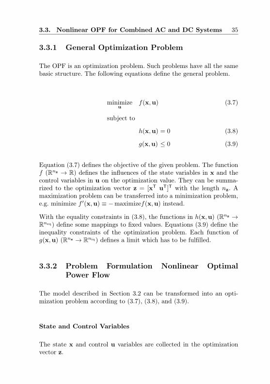
3.3. Nonlinear OPF for Combined AC and DC Systems 35
3.3.1 General Optimization Problem
The OPF is an optimization problem. Such problems have all the samebasic structure. The following equations define the general problem.
minimizeu
f(x,u) (3.7)
subject to
h(x,u) = 0 (3.8)
g(x,u) ≤ 0 (3.9)
Equation (3.7) defines the objective of the given problem. The functionf (Rnz → R) defines the influences of the state variables in x and thecontrol variables in u on the optimization value. They can be summa-rized to the optimization vector z = [xT uT]T with the length nz. Amaximization problem can be transferred into a minimization problem,e.g. minimize f ′(x,u) ≡ −maximizef(x,u) instead.
With the equality constraints in (3.8), the functions in h(x,u) (Rnz →Rneq) define some mappings to fixed values. Equations (3.9) define theinequality constraints of the optimization problem. Each function ofg(x,u) (Rnz → Rniq) defines a limit which has to be fulfilled.
3.3.2 Problem Formulation Nonlinear OptimalPower Flow
The model described in Section 3.2 can be transformed into an opti-mization problem according to (3.7), (3.8), and (3.9).
State and Control Variables
The state x and control u variables are collected in the optimizationvector z.

36 Chapter 3. Optimal Power Flow for MTDC Grids
z =
x
u
(3.10)
x =
uAC
uACc
uDC
θ
θc
(3.11)
u =
pgen
qgen
qsvc
a
ϕ
pACvsc
qvsc
(3.12)
The state variables of the AC grid are the voltage magnitudes uACk and
voltage angles θk ∀ k = 1, . . . , nACbus for each bus in the AC grid. Accord-
ing to Figure 3.1, each converter adds two additional buses to the ACgrid and therefore also to the state vector. This means uAC
c = [uACc1 uAC
c2 ]and θc = [θc1 θc2] ∀ c = 1, . . . , nvsc need to be added to the state vector.The DC grid can be defined by the voltages uDC
i ∀ 1, . . . , nDCbus, which
are added to the state vector.
The variables in vector u are controllable. It depends on the marketmodel, to which extent the ISO has control over them. The generalapproach presented, considers full control. There is the possibility toconstrain each of the variables to fixed values, as explained later on.With this approach a hybrid grid which may include uncontrollablerenewable and controllable generators can be assessed. Excluding theslack generator to balance the grid, all other generators can have a

3.3. Nonlinear OPF for Combined AC and DC Systems 37
fixed generation, and then only the power setpoints of the convertersare free to control.
The active power generation pgen,p ∀ p = 1, . . . , ngen for each generatorare the first control variables. The generators could be located eitherin the AC grid or in the DC grid. qgen,p ∀ p = 1, . . . , nAC
gen containsall variable to control the reactive power in the generators of the ACgrid. The static var compensator (SVC) are represented by qsvc,k ∀ k =1, . . . , nsvc. The controllable transformers are defined by the tap ratioakm of line k to m. There are ntap tap changing transformers in thegrid. The npha phase shifting transformers in the grid are defined withϕkm. With the described variables the AC and DC grid are definedindividually, but not linked together.
Finally the converter power flows are added to the vector u. They linkthe AC and DC systems together. In this optimization, the flow on theAC grid side of the converter is controlled, so pAC
vsc,c ∀ c = 1, . . . , nvsc isadded to u. It would also be possible to control the power on the DCside, but since they are linked with (3.3), this would have the same influ-ence on the optimization. The reactive power output of the convertersqvsc,c ∀ c = 1, . . . , nvsc is added as the last entry in u.
The number of variables nx depends on the system size. The maximallength of x is nx and can be calculated according to the entries of x. Asimilar approach can be used for u.
nx =nACbus + 2nvsc + nDC
bus + nACbus + 2nvsc
= 2nACbus + nDC
bus + 4nvsc (3.13)
nu =ngen + ngen + nsvc + ntap + npha + nvsc + nvsc
= 2ngen + 2nvsc + nsvc + ntap + npha (3.14)
nz =nx + nu
= 2nACbus + nDC
bus + 6nvsc + 2ngen + nsvc + ntap + npha (3.15)
If all described variables are specified, the system is over defined. De-pending on the implementation of the problem, the vector x can bereduced. The removed state variables change to algebraic states whichstill have to fulfill certain limits. The DC voltages uDC can be reduced

38 Chapter 3. Optimal Power Flow for MTDC Grids
to one voltage per DC grid, since all others are defined by the exchangedpower by the AC and DC grid. The voltage and phase angle at all busesc2 can be removed, since they are determined by the active and reactiveflows through the converters pAC
vsc,c and qvsc,c. One voltage angle can beset to 0, which acts as reference bus. The active power flow through oneconverter pAC
vsc,c can be removed from the vector u, since it is the onlyconverter with a DC voltage. This ensures the power balance over theDC grid.
3.3.3 Objective Function
Different objectives are possible in a combined AC and DC grid. Themost important examples are shown below.
minimizeu
f(x,u) (3.16)
where
f(x,u) =
ngen∑p=1
αgen,p + βgen,ppgen,p + γgen,p
(pgen,p
)2
(3.17)
Equation (3.17) is the most common one. The generation cost are cal-culated according to a quadratic cost model, with αgen,p as fix cost, andminimized. This cost terms are included to calculate the full produc-tion cost. They can be neglected for the optimization, but this will givean offset to the optimization value. The values βgen,p and γgen,p definethe linear and quadratic cost for the active power production of eachgenerator p. The second proposed objective is described in (3.18).
f(x,u) =
ngen∑p=1
pgen,p (3.18)
This approach minimizes the overall production in the grid, howeverdifferences in the production cost are not considered. With this objec-tive, the overall losses are minimized, since they can be influenced bychanging the generation dispatch and especially the converter setpoints.It is also possible to operate the grid as close as possible to a predefinedprofile.

3.3. Nonlinear OPF for Combined AC and DC Systems 39
f(x,u) =
nACbus∑k=1
(uACk − uAC
set,k
)2
+
nDCbus∑i=1
(uDCi − uDC
set,i
)2
(3.19)
Equation (3.19) gives an example to follow a given voltage profile asclose as possible. The distance to the set values uAC
set,k and uDCset,i are
penalized with a quadratic term. Also other deviations as voltage angles,power flows, generation, etc. could be used as variables for this objectivefunction. The last example given in (3.20) is a more exotic objectivefunction to show other possibilities.
f(x,u) =
nvsc∑c=1
(Π(pACvsc,min,c − pAC
vsc,c
)+
Π
pACvsc,max,c − pAC
vsc,min,c
(pACvsc,c − pAC
vsc,min,c
)2)
(3.20)
The idea is to have an optimal flexibility in the converter stations. Thepower setpoints of the converter pAC
vsc,c are penalized, if they are awayfrom the middle between maximum power setpoint pAC
vsc,max,c and mini-mum power setpoint pAC
vsc,min,c. The parameter Π defines the shape of thecurve. A higher Π means more curved penalty function, see AppendixA. This objective could also be added as a second term, e.g. to (3.17).
Other objective functions are also possible. This is dependent on thesystem and the control objective of the operator.
3.3.4 Equality Constraints
There are three different types of equality constraints summarized in(3.8). The first type is the AC bus power balances. Each bus k ∀ k =1, . . . , nAC
bus in the AC grid must fulfill the active and reactive powerbalance:
pACgen,k − pAC
load,k − pAClin,k − pAC
vsc,k = 0 (3.21)
qgen,k − qload,k − qlin,k − qvsc,k = 0 (3.22)

40 Chapter 3. Optimal Power Flow for MTDC Grids
pgen,k is the sum of all generator’s active power infeed at bus k. pload,k isthe sum of all active power loads at bus k. The transfer of active powerover any line or transformer away from bus k are represented by pAC
lin,k.If a converter is connected to bus k, pAC
vsc,k has to be added. The samesubscripts are used for the reactive power balance.
The same is valid for the DC grid. Each DC bus must also fulfill thepower balance:
pgen,i − pload,i − pDClin,i − pDC
vsc,i = 0 (3.23)
The second type of equality constraint is the power balance of the con-verters. A reformulation of (3.3) gives the next equality constraint:
pACvsc,c − pDC
vsc,c + ploss,c = 0 (3.24)
The last equality constraints are for the reference buses. Since multipleasynchronous AC grids could be connected with an MTDC grid, eachof these AC grids needs one reference bus. There the voltage angle isfixed to a defined value, usually
θk − θref,k = 0 (3.25)
where k is the reference bus, separate for each AC grid. The DC griddoes not need a reference bus in this formulation.
3.3.5 Inequality Constraints
In addition to the equality constraints, also inequality constraints arebounding the problem. Most of them represent the physical limits of thedevices used in the combined grid. The first constraints are the powerline ratings. The flow on each AC and DC line has to stay below theirtransmission capacity. Usually the current is the limiting value on thelines, therefore the apparent power needs to be constrained. Due to thelosses, flows at both ends of a line need to be considered.

3.3. Nonlinear OPF for Combined AC and DC Systems 41
sACmin,km ≤ sAC
km ≤ sACmax,km (3.26)
sACmin,mk ≤ sAC
mk ≤ sACmax,mk (3.27)
To simplify the problem and reduce the computational complexity, theactive and reactive power can be constrained instead of the apparentpower.
pACmin,km ≤ pAC
km ≤ pACmax,km (3.28)
pACmin,mk ≤ pAC
mk ≤ pACmax,mk (3.29)
qmin,km ≤ qkm ≤ qmax,km (3.30)
qmin,mk ≤ qmk ≤ qmax,mk (3.31)
The DC line limits also need to be incorporated.
pDCmin,ij ≤ pDC
ij ≤ pDCmax,ij (3.32)
pDCmin,ji ≤ pDC
ji ≤ pDCmax,ji (3.33)
The next inequality constraints are the active and reactive power out-put of the generators. The reactive and active power limits are coupledto each other. According to [58], there are three limitations: the fieldcurrent, the armature current, and the end region heating limits. Theylimit the possible output according to Figure 3.3. The feasible outputis inside the curve, marked as grey area, which can be approximated asintersection of three circles and the half plane right of the x-axis.
A simplification is to use only box constraints. In general, the constraintscan be formulated as:
0 ≤ pgen,min,p
(qgen,p
)≤ pgen,p ≤ pgen,max,p
(qgen,p
)(3.34)
qgen,min,p
(pgen,p
)≤ qgen,p ≤ qgen,max,p
(pgen,p
)(3.35)

42 Chapter 3. Optimal Power Flow for MTDC Grids
pf=0.95 lead
pf=0.85 lag
pgen,max
qgen,max
Ove
rexc
ited
Und
erex
cite
d
Field currentheating limits
Armatur currentheating limits
End regionheating limits
0 pgen
qgen
Figure 3.3: Capability curve of a generator according to [58]. There arethree different limitations of a generator output: the fieldcurrent, the armature current, and the end region heatinglimits.
The voltage ratings of the buses give the next inequalities. Each busvoltage in the AC and DC grid must be inside its feasibility range.
uACmin,k ≤ uAC
k ≤ uACmax,k (3.36)
uDCmin,i ≤ uDC
i ≤ uDCmax,i (3.37)
The controllable devices in the system do also have their control range.The SVC has a range for reactive power.
qsvc,min,k ≤ qsvc,k ≤ qsvc,max,k (3.38)
The tap changing transformers are also limited in range and to discretevalues. Since the steps are usually rather small, the function is chosencontinuous to simplify the optimization. The phase shifting transformers

3.3. Nonlinear OPF for Combined AC and DC Systems 43
have a defined operation range, in which it can influence the voltageangle between the buses where it is connected.
amin,km ≤ akm ≤ amax,km (3.39)
ϕmin,km ≤ ϕkm ≤ ϕmax,km (3.40)
The flow through the converter is limited by the current in the valves,which is limited with the following equation [60].
|sc| ≤ |uc2iACmax,c| (3.41)(
pACc
)2
+(qc
)2
≤(uc2i
ACmax,c
)2√3 (3.42)
Beside that the VSC can generate or consume reactive power by con-trolling the θc2 , zc is a reactive element, 1/zc = yc=gc + jbc ≈ jbc.Therefore, the flow equation is given by:
qmax,c = −bc2c1(uAC
max,c2
)2
+ uACmax,c2u
ACc1 bc2c1 cos
(θc2 − θc1
)(3.43)
The minimum reactive power of a VSC station is limited to a percentage,kc, of the rated nominal power [65].
qc,min = −kcpACvsc,nom,c (3.44)
Equations (3.41) to (3.44) limit the output of a VSC station to thefeasible region, as shown in Figure 3.4.
This results in a summarized inequality for the VSC stations flows.
pACvsc,min,c
(qvsc,c
)≤ pAC
vsc,c ≤ pACvsc,max,c
(qvsc,c
)(3.45)
qvsc,min,c
(pACvsc,c
)≤ qvsc,c ≤ qvsc,max,c
(pACvsc,c
)(3.46)

44 Chapter 3. Optimal Power Flow for MTDC Grids
pAC (p.u.)
q(p.u.)
0
Max apparentpower
Min reactivepower
Max reactivepower exactand simplified
pACmaxpAC
min
qmax
qmin
Figure 3.4: Capability curve of a VSC station. Limited by the ap-parent power (red circle), minimal (green line) and maxi-mal reactive power (light blue arc). The maximal reactivepower can be simplified by a linear approximation (dashedblue line).
3.4 Linearized Optimal Power Flow forCombined AC and DC Systems
The above described optimal power flow problem includes no approx-imations. However, it is nonlinear and non-convex and therefore oftenhard to solve. Iterative solvers need to be applied, which are computa-tionally expensive and it is not possible to guarantee a global minimum.An approach which tries to find global minimum for mixed AC and DCproblems is presented in [66]. However, it is often possible to simplifythe problem by linearizing it. The price is the reduced accuracy andneglecting the reactive power part, as well as the losses. This modelis often called DC power flow model in literature. Since they are notrelated with physical DC grids, this term is confusing and in this thesisthey are referred to as linearized power flow methods.

3.4. Linearized OPF for Combined AC and DC Systems 45
The perceived advantages achieved by using a linearized model are sum-marized in [67]:
• its solutions are non-iterative, unique and reliable.
• its software and methods are straightforward to implement.
• its models can be optimized and solved efficiently, particularlyregarding contingency analysis.
• needed network data is less than for nonlinear AC methods.
• its linearity fits to the economic theory on which plenty of thetransmission-oriented market design is based today.
• its approximated active power flows are reasonably accurate, whensystem load is not too high.
The first two methods of linearized power flow models were presented in[68] and [69]. Several developments and additional features were addedover the years and there is still research going on in this topic. A goodoverview is given in [67].
According to the author’s knowledge up to now, there are either modelswith AC existing or they include only DC point-to-point connections [54]or have predefined power setpoints for the converters [70]. A methodto incorporate also MTDC was presented by the author in [43] andexplained in the next section.
3.4.1 General Optimization Problem with Quad-ratic Objective and Linear Constraints
The linearized OPF problem has the same structure as the general op-timization problem stated in (3.7) - (3.9). The objective function ishere represented by a quadratic function. All equality and inequalityconstraints are linearized and given in matrix form.
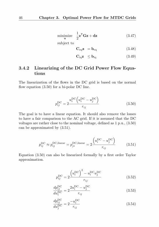
46 Chapter 3. Optimal Power Flow for MTDC Grids
minimizeu
1
2zTGz + dz (3.47)
subject toCeqz = beq (3.48)
Ciqz ≤ biq (3.49)
3.4.2 Linearizing of the DC Grid Power Flow Equa-tions
The linearization of the flows in the DC grid is based on the normalflow equation (3.50) for a bi-polar DC line.
pDCij = 2
uDCi
(uDCi − uDC
j
)rij
(3.50)
The goal is to have a linear equation. It should also remove the lossesto have a fair comparison to the AC grid. If it is assumed that the DCvoltages are rather close to the nominal voltage, defined as 1 p.u., (3.50)can be approximated by (3.51).
pDCij ≈ p
DC,linearij = pDC,linear
ji = 2
(uDCi − uDC
j
)rij
(3.51)
Equation (3.50) can also be linearized formally by a first order Taylorapproximation.
pDCij = 2
(uDCi
)2
− uDCi uDC
j
rij(3.52)
dpDCij
duDCi
= 22uDC
i − uDCj
rij(3.53)
dpDCij
duDCj
= 2−uDC
i
rij(3.54)

3.4. Linearized OPF for Combined AC and DC Systems 47
Inserting the operation point of uDC0,i = 1 p.u. and uDC
0,j = 1 p.u. leadsto:
pDCij[uDC
0,i ,uDC0,i
] = 0 (3.55)
dpDCij[uDC
0,i ,uDC0,i
]duDC
i
=2
rij(3.56)
dpDCij[uDC
0,i ,uDC0,i
]duDC
j
=−2
rij(3.57)
Applying the Taylor series at the operation point results in the followingequation:
PDC,linearij = pDC
ij[uDC
0,i ,uDC0,i
]++ ∆uDC
i
dpDCij[uDC
0,i ,uDC0,i
]duDC
i
+ ∆uDCj
dpDCij[uDC
0,i ,uDC0,i
]duDC
j
= 0 + 2(uDCi − 1
) 1
rij+ 2(uDCj − 1
)−1
rij
= 2
(uDCi − uDC
j
)rij
(3.58)
The mathematical approximation (3.58) is the same as the one in (3.51).This equation is used to approximate the power flows in the linearizedmodel. The DC voltages are then only relative values considering areference voltage.
The power flow error epDCij
can be approximated by assuming a line froma DC bus with the highest voltages allowed in the grid uDC
max to one withthe lowest voltage uDC
min.

48 Chapter 3. Optimal Power Flow for MTDC Grids
epDCij
= pDCij − p
DC,linearij (3.59)
epDCij ,max =
uDCmax
(uDC
max − uDCmin
)rij
−
(uDC
max − uDCmin
)rij
=
(uDC
max − 1)(uDC
max − uDCmin
)rij
(3.60)
The relative error erelativepDCij
can then be calculated as following.
erelativepDCij ,max =
epDCij ,max
pDCij
=uDC
max − 1
uDCmax
(3.61)
Assuming a symmetric voltage band of ±5 % around the nominal volt-age, which means ± 16 kV for a 320 kV line, the maximum relativepower flow error erelative
pDCij ,max according to (3.61) is only 4.76 %. If the volt-
age band is increased to ±10 %, which is already high for a VSC for longterm analysis, the worst case flow error increases to 9.09 %, which is stilla reasonable approximation for such an extreme case. If the minimumand maximum voltage are exchanged with each other, the same valuesoccur for the errors. In most cases the voltage deviations are rarely atthat extreme values, since the highest and lowest voltage do not occurnext to each other. Therefore, the errors are smaller in practice.
3.4.3 Problem Formulation Linear Optimal PowerFlow
The state and control variables, the objective function and the equal-ity and inequality constraints of the linearized OPF formulation areexplained below.

3.4. Linearized OPF for Combined AC and DC Systems 49
State and Control Variables
The optimization vector z is divided into state x and control variablesu. The reduced complexity of the system, also reduces the size of vectorx. The states of the AC grid are only the voltage angles θk ∀ k =1, . . . , nAC
bus. The voltages in the AC grid are assumed as 1.0 per-unit(p.u.) and therefore not calculated. Consequently, the transformer inthe VSC station shown in Figure 3.1 can be removed. Since the lossesare neglected, the line from c1 to c2 can also be removed. In that case theconverter is modeled as a special generator connected directly to the bus.The DC grid is defined by the voltage deviations ∆uDC
i ∀ i = 1, . . . , nDCbus.
The control variables are reduced to the active power generation pgen,p ∀1, . . . , ngen. The same can be said as above all not controllable generatorscan be fixed to a value and removed from the optimization vector. Tohave a fair comparison with the AC grid, also the physical losses in theconverters are neglected and therefore pAC
vsc,c = pDCvsc,c = pvsc,c ∀ c =
1, . . . , nvsc for the linearized OPF.
z =
x
u
(3.62)
x =
θ
uDC
(3.63)
u =
pgen
pvsc
(3.64)
The reduction of variable types leads to a reduction of the number ofvariables in the vectors x and u, too.
nx = nACbus + nDC
bus (3.65)
nu = ngen + nvsc (3.66)
nz = nx + nu
= nACbus + nDC
bus + ngen + nvsc (3.67)


3.4. Linearized OPF for Combined AC and DC Systems 51
minimizeu
f(x,u) (3.68)
where
f(x,u)=
ngen∑p=1
αgen,p + βgen,ppgen,p + γgen,p
(pgen,p
)2
+∑
km∈ΩAC
πACkm
(θk − θm
)2
+∑
ij∈ΩDC
πDCij
(uDCi − uDC
j
)2
(3.69)
+
nvsc∑c=1
πvsc,c
(pvsc,c
)2
The set ΩAC includes all pairs of AC buses k and m, which have a directline between them. ΩDC is the corresponding set in the DC grid. Theterm πAC
km is an individual penalty factor for each line. The losses are de-pendent on the conductance gkm of the line, compare (3.1). In linearizedpower flows, usually only the conductance is available. Therefore, it isreasonable to penalize the flows in the AC grid in reverse to the value ofthe conductance gkm. In the DC grid the resistance is the value whichdefines the losses. Therefore πDC
ij is dependent on rij . πvsc,c representsthe losses of the converters. There could be different types of converters,thus πvsc can have different values at each converter.
πACkm = πscaleπ
ACgkm (3.70)
πDCij = πscaleπ
DC rij (3.71)
πvsc,c = πscale
ploss,c
(pvsc,c
)pvsc,c
(3.72)
The factor πscale is chosen in such a way, that the generation cost,which is represented by the first factor in (3.69), is by far predominantcompared to the penalty terms, which are represented by the secondfactor in (3.69). The second term at (3.72) is pre-defined at a specific

52 Chapter 3. Optimal Power Flow for MTDC Grids
power throughput, according to (3.4) and (3.5). If the approximatedphysical losses of the grid are known, the ratio between the losses and thetotal generation is known. In such a case πscale can be chosen, that theratio of the penalty factors to the total cost be of the same magnitudeas the physical losses to the generation.
This approach can also be applied to other objective functions to opti-mize different goals in the combined AC and DC grid.
Equality Constraints
The equality constraints are mainly the same as in the nonlinear case.Positive flows of pvsc are defined from the AC into the DC grid. For ACand DC grid one gets
pACgen,k−pAC
load,k−pAClin,k−pvsc,k = 0 (3.73)
pDCgen,i−pDC
load,i−pDClin,i +pvsc,i = 0 (3.74)
Equations (3.73) and (3.74) can be written in matrix form.
Ceqz = beq (3.75)
where
Ceq =
−BAC 0 HAC T
0 −BDC HDC S
(3.76)
beq = pload (3.77)
The first row corresponds to the power balances at the AC nodes. Thesecond row is the respective equation in the DC grid. The matrices BAC
and BDC are the admittance matrices for each grid. HAC and HDC
are the generators distribution matrices, which allocate the generationcapacity to each bus. T and S define the positions of the converter inthe AC and DC grid. The detailed construction of these matrices isexplained in the Appendix B. The equality vector beq consists of thetotal load at each node for all AC and DC nodes.

3.4. Linearized OPF for Combined AC and DC Systems 53
Still a reference voltage angle is needed. The angle at the defined busper AC area is set to zero. The DC grid is now modeled in a similar wayas the AC grid and requires also a reference bus for each MTDC grid.At this DC bus the voltage reference point is set and only the deviationsfrom this voltage are considered.
θk −θref,k = 0 (3.78)
uDCi −uDC
ref,i = 0 (3.79)
The rows corresponding to the reference angle and voltage can be re-moved in (3.76).
Inequality Constraints
The inequality constraints of the linearized system are concerning thetransferred power over each transmission line, either in the AC or DCgrid. Only the active power is considered. As a consequence of neglectingthe losses, only the flow in one direction has to be verified, since it hasthe same value to the other direction.
pACmin,km ≤ pAC
km ≤ pACmax,km (3.80)
pDCmin,ij ≤ pDC
ij ≤ pDCmax,ij (3.81)
The next constraints affect the active power output of the generators inthe AC and DC grid. Here the minimum is greater or equal to zero.
0 ≤ pgen,min,p ≤ pgen,p ≤ pgen,max,p (3.82)
The power transfer of the VSC stations is also constrained. The con-verter constraints are usually symmetrical.
pvsc,min,c ≤ pvsc,c ≤ pvsc,max,c (3.83)
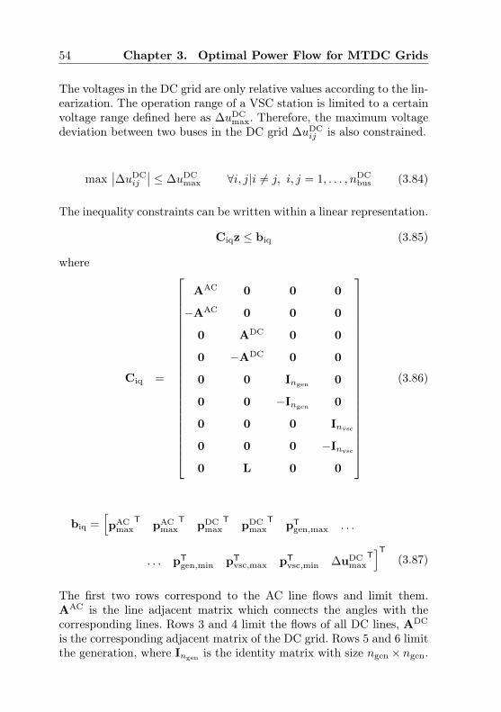
54 Chapter 3. Optimal Power Flow for MTDC Grids
The voltages in the DC grid are only relative values according to the lin-earization. The operation range of a VSC station is limited to a certainvoltage range defined here as ∆uDC
max. Therefore, the maximum voltagedeviation between two buses in the DC grid ∆uDC
ij is also constrained.
max∣∣∆uDC
ij
∣∣ ≤ ∆uDCmax ∀i, j|i 6= j, i, j = 1, . . . , nDC
bus (3.84)
The inequality constraints can be written within a linear representation.
Ciqz ≤ biq (3.85)
where
Ciq =
AAC 0 0 0
−AAC 0 0 0
0 ADC 0 0
0 −ADC 0 0
0 0 Ingen 0
0 0 −Ingen 0
0 0 0 Invsc
0 0 0 −Invsc
0 L 0 0
(3.86)
biq =[pAC
maxT
pACmax
TpDC
maxT
pDCmax
TpT
gen,max . . .
. . . pTgen,min pT
vsc,max pTvsc,min ∆uDC
maxT]T
(3.87)
The first two rows correspond to the AC line flows and limit them.AAC is the line adjacent matrix which connects the angles with thecorresponding lines. Rows 3 and 4 limit the flows of all DC lines, ADC
is the corresponding adjacent matrix of the DC grid. Rows 5 and 6 limitthe generation, where Ingen is the identity matrix with size ngen × ngen.

3.5. Case Study of Nonlinear and Linear OPF 55
Rows 7 and 8 limit the flows through the converters, where Invsc is anidentity matrix with the corresponding size. The matrix L limits themaximum voltage deviations in the DC grid. The detailed constructionof the matrices for the inequality constraints is given in Appendix B.
3.5 Case Study of Nonlinear and Linear Op-timal Power Flow
A case study for a small test grid is given here. Case studies on a largegrid, comparing all proposed methods, are given in Chapter 5.
3.5.1 Study Grid Topology
The used test system is shown in Figure 3.6. It is based on the IEEE14bus power flow test case, available at [71] combined with an overlayMTDC grid. The topology of the DC grid is not optimized for the oper-ation of this combined grid, but rather chosen as one typical possibility.In this thesis, the planning problem was not addressed. This is subjectof future research.
The grid has 14 AC buses (1 to 14) and five DC buses (DC1 to DC5).The DC bus DC5 is not directly connected to the AC grid. Therefore,there are four converter stations C1 to C4 integrated in the grid. Thecombined grid consists of six generators G1 to G6, of which five arein the AC grid and one is connected directly to the DC grid. Thiscould represent for example a wind park, but it is also imaginable thatlarge conventional generators will be connected directly to future MTDCgrids. The total load is 2.59 p.u., of which the major loads are connectedin the south of the grid. No load is connected directly to the MTDCgrid, even if this would be possible. The AC buses are connected with20 lines, of which five are transformers, including one phase shifter frombus 5 to bus 6. The DC grid has seven transmission lines. The detailedgrid data is available in Appendix C.
3.5.2 Test Environment
The above described test system is used to show the difference in the de-rived OPF formulations. Three different cases are simulated: the nonlin-

56 Chapter 3. Optimal Power Flow for MTDC Grids
1
2 3
4
5
6
78
9
101112
1314
DC1
DC2
DC3
DC4
DC5
G1
G2
G3
G4
G5G6
C1
C2
C3
C4
AC Bus AC Line Generator Load
DC Bus DC Line Transformer VSC
Figure 3.6: IEEE14 bus test case (black) with 20 AC lines and fivegenerators is extended by an MTDC grid (green) includingfour converters, five DC buses, seven DC lines and oneadditional generator.
ear case based on Section 3.3 and two linearized cases based on Section3.4. The two latter cases are distinguished by the chosen loss penaltyterms to show the important influence of them. The actual values aregiven in Table 3.1. In the “Base” case the line flow values are set to 1and the converter penalties to 0.001. In that way a even distributionresults. In the “Suitable” case the values are adjusted to the real lossesin the grid. The high number for πDC originates in the p.u. calculation.The voltage values are scaled by a base voltage of 380 kV. The differ-ences of the voltages are also squared. Therefore, the penalties for theDC lines have to be scaled with a large factor. The converter penalties

3.5. Case Study of Nonlinear and Linear OPF 57
Table 3.1: Penalty terms for the two different cases simulated with thelinear OPF.
Parameter Suitable Base
πscale 1.2·101 1·100
πAC 1·100 1·100
πDC 5·109 1·100
πvsc 1·10−2 1·10−3
are set to 1 % which represents typical losses. The general scaling factorπscale was set to 12. This value was found during several simulations. Itsets the overall penalty cost to about 3.5 % of the total generation cost,which gives the penalty terms a weight similar to the expected losses ascalculated by the nonlinear version.
The solver used for the nonlinear case is the fmincon Matlab functionwith the sequential quadratic programming (SQP) algorithm. The lin-earized version is optimized by using the quadprog function with aninterior-point-convex algorithm. The solver time (average of five) forthe cases was 1054.64 ms for the nonlinear case and 15.09 ms for thelinear case on a standard desktop computer (Intel Core 2 Quad Q95502.83 GHz, 8 GB Ram) within a Matlab environment. The calculationtime is given to show the calculation ratio. The calculation in generalcould be faster by using more optimized problem solvers, faster pro-gramming environments, or more up to date hardware, but this was notthe scope here.
3.5.3 Simulation Results
Costs
The production cost for the three cases in monetary units (m.u.) areshown in Figure 3.7. The highest cost is produced by the nonlinear case.The generation cost, represented by the filled bars in Figure 3.7, areabout 3.5 % lower for both linearized cases. This is not surprising, sincein the nonlinear case the losses have to be compensated by generation.

58 Chapter 3. Optimal Power Flow for MTDC Grids
37.5
40.0
42.5
45.0
47.5
50.0
Cost
(m.u.)
Nonlinear OPF
Linearized OPF suitable penalties
Linearized OPF base penalties
37.5
40.0
42.5
45.0
47.5
50.0
Cost
(m.u.)
Nonlinear OPF
Linearized OPF suitable penalties
Linearized OPF base penalties
Figure 3.7: Comparison of costs in m.u. for the nonlinear and lin-earized OPF in the IEEE14 bus test grid, with an addedMTDC system. The filled areas correspond to the genera-tion cost, and the striped area represent the penalty terms.
If the penalty cost is added, shown with the striped area, the cost forthe suitable penalty case is about the same range as in the nonlinearcalculation. The flat penalty case has almost no added cost, even withthe magnification in Figure 3.7, only a thin line is seen. It shows that thegeneration cost are approximately the same for the base and suitablecase.
Generators
The cost originates from the generation pattern. The different gener-ation patterns in per-unit (p.u.) are shown in Figure 3.8. GeneratorG6 placed in the DC grid is the cheapest one. In all cases it is at itsmaximum capacity. The difference lies in the generation of G1 and G2,since the other AC generators are much more expensive. The linear casewith suitable penalties is close to the nonlinear case. Its production isa bit lower since no losses needed to be compensated. The base penaltycase shows remarkable deviations, since it is hard to distinguish betweengenerator G1 and G2, because their production costs are close (see Ta-ble C.5). This indicates that the penalty terms have a large influenceon the result.

3.5. Case Study of Nonlinear and Linear OPF 59
G1 G2 G3 G4 G5 G60.0
0.2
0.4
0.6
0.8
1.0
1.2
1.4
1.6
Generator number
Pow
erflo
w(p.u.)
Nonlinear OPFLinearized OPF suitable penaltiesLinearized OPF base penalties
Figure 3.8: Comparison of generated power for all six generators be-tween nonlinear version and linearized OPF in the IEEE14bus test grid, with an added MTDC system. G1-G5 areplaced in the AC grid and G6 is connected directly to theDC grid.
Converter Stations
The same behavior is observed for the converter powers, as shown inFigure 3.9. In all three cases the same general flow pattern is the same:infeed to the DC grid at converter C1 and the generator G6 in the DCgrid, and absorption at all other converters. The transfered powers inthe nonlinear OPF and the suitable penalty case are close together withsmall deviations in both directions. Whereas the base penalty case isonly close for converter C2 and C3 and deviates a lot for C1 and C4.
DC and AC transmission lines
The power transfers through the converters of the DC grid are dis-tributed over the seven DC lines. In all three cases the flow in DC line 4connecting buses DC2 and DC5 is at the capacity limit. This is becausethe cheap generation at bus DC5 and the large load at AC bus 3. Ingeneral, the flow pattern for the first two cases are close together andthe last case has some deviation. The major grid flow direction has to

60 Chapter 3. Optimal Power Flow for MTDC Grids
C1 C2 C3 C4−0.75
−0.50
−0.25
0.00
0.25
0.50
0.75
Converter number
Con
vert
erpo
wer
(p.u
.)
Nonlinear OPFLinearized OPF suitable penaltiesLinearized OPF base penalties
Figure 3.9: Comparison of power flow through converters betweennonlinear version and linearized OPF in the IEEE14 bustest grid, with an added MTDC system. The infeed to theMTDC grid is at C1 and from G6 placed directly in theDC grid.
be in line with the converter flows. Besides the full loaded line DC2 toDC5, the flow in the DC grid has another major direction, from busDC1 to DC4. We can conclude that generator G1 supplies the north-ern part of the grid and generators G2 and G6 supply load 3 and thesouthern and eastern part of the grid loads.
Figure 3.11 shows the flows in all 20 AC lines. The pattern between thethree cases is also recognizable here. The nonlinear case is most of thetime close to the linearized OPF with suitable penalty factors and thecase with the base penalties is further away.

3.5. Case Study of Nonlinear and Linear OPF 61
DC1-D
C4
DC1-D
C5
DC2-D
C3
DC2-D
C5
DC3-D
C4
DC3-D
C5
DC4-D
C5−0.6
−0.4
−0.2
0.0
0.2
0.4
0.6
DC line from - to
Pow
erflo
w(p.u.)
Nonlinear OPFLinearized OPF suitable penaltiesLinearized OPF base penalties
Figure 3.10: Comparison of power flow through DC lines between non-linear version and linearized OPF in the IEEE14 bus testgrid, with an added MTDC system.
1 2 3 4 5 6 7 8 9 10 11 12 13 14 15 16 17 18 19 20−0.4
−0.3
−0.2
−0.1
0.0
0.1
0.2
0.3
0.4
0.5
AC line number
Pow
erflo
w(p.u.)
Nonlinear OPFLinearized OPF suitable penaltiesLinearized OPF base penalties
Figure 3.11: Comparison of power flow through AC lines between non-linear version and linearized OPF in the IEEE14 bus testgrid, with an added MTDC system.

62 Chapter 3. Optimal Power Flow for MTDC Grids
3.6 Conclusion
In this chapter the OPF problem is extended to incorporate DC grids.For TSOs to operate a future grid which includes combined AC andmeshed DC grids such a problem must be solved.
First, the full power flow equations are used and a nonlinear model ofthe DC grid is added to represent the flows as accurate as possible. Aconverter model is used to link both grids. The losses are also calculatedaccording to a flow based loss model.
Second, the same problem was analyzed using a linearized model. Theflows in the DC grid are linearized with an approximation, wherebythe error in the extreme case is maximal 9 % compared to the nonlin-ear model. This value will rarely occur in practice. This linearized flowmodel has no physical losses in the lines, therefore also the losses in theconverter needed to be removed for consistency reasons. To compen-sate this effect and ensure the balancing between the AC and DC, gridpenalty terms are added to the objective function to model losses in thetransmission lines and the converters.
The case study shows that the linearized method works well for cost,generation, converter and line flows, if the penalty terms are chosenin such a way, that they are on a similar level as the physical losseswould be. The penalty factors can be tuned according to the availableparameters of the grid. A scaling is required to reach an appropriatelevel of simulated losses. Of course this depends on the grid structureand size.
The operation of a grid with the proposed optimization could lead tosevere problems, if a contingency arises in the combined grid. Therefore,security aspects need to be added to the optimization, which is done inthe next chapter.

Chapter 4
Security ConstrainedOptimal Power Flow forMulti-Terminal HVDCGrids
The reliable and secure operation of a transmission system, under con-sideration of the costs, is the core goal of each TSO. To schedule theflows an OPF can be applied which also considers the security as-pects. This chapter investigates the security constrained optimal powerflow (SCOPF) considering the N-1 criterion. This means that each ACand DC line can have an outage as well as all generators, without vio-lating any constraint in the system. In addition to this standard imple-mentation, this chapter considers the fact that also converters can fail,and significantly influence the flows in the AC and DC grid. There aretwo ways to react to a contingency, either in a preventive or correctiveway. Both methods are considered in this chapter. First the SCOPF for-mulation is explained, followed by a small case study. This chapter isbased on [72] and [73].
63

64 Chapter 4. SCOPF for MTDC Grids
4.1 Introduction to Security ConstrainedOptimal Power Flow
The secure operation of a power grid is an old topic. A definition ofsteady state security, which is here addressed, is given in [74]. It isdefined as: “The ability of the system to operate steady-state-wise withinthe specified limits of safety and supply quality following a contingency,in the time period after the fast-acting automatic control devices haverestored the system load balance, but before the slow-acting control, e.g.transformer tapping and human decisions, have responded.”
The used approach is the N-1 criterion, which is defined according to [75]as: “The rule according to which elements remaining in operation withinTSOs responsibility area after a contingency from the contingency listmust be capable of accommodating the new operational situation withoutviolating operational security limits.” This basically means that eachsingle element can fail and the system still has to operate properly.A probabilistic approach including MTDC grids was presented by theauthor in [76] which is beyond the scope of this thesis.
Each new component added to the grid needs to be considered withregard to these formulations. An overview over the existing AC gridSCOPF formulations is given in [77], and in a more recent version in[78].
The DC grid is much more than just an additional element placed in thegrid, because it has more the structure of a parallel power system. All ofthe DC grid elements have to be studied, by taking into considerationthat they can have an outage. The advantage of the DC grid is the fastcontrollability of the power flows through the converters. This abilitycan be used to relief the stress from the grid after a contingency eitherin the DC or in AC grid.
As the N-1 criterion definition above explains there are some fast-actingcontrollers in the AC grid, but the grid security is planned in a preven-tive way. This means the grid flow reacts passively without control. Ittakes some time before the slow-acting controllers operate. The VSCadd fast controllability to the grid which can influence the power flowsin short time scales. This flexibility can be used to act after a contin-gency. This so called corrective control allows to use more of the gridcapacity during nominal operation, since the reserve margins can besmaller.

4.2. Nonlinear SCOPF for Combined AC and DC Grids 65
In general, there are two kinds of control action possible in the powergrid, the preventive and the corrective actions. The preventive actionis defined as actions which are taken before a contingency occurs inthe grid. The controllable devices are used to set up the grid in sucha way, that it can withstand any contingency and the new power flowsdo not violate any constraints. The corrective control is applied after acontingency has happened in the grid. The control actions, which can beprecalculated, change the power flow in the system after the contingencyto bring the system back to a stable operation point. For this kind ofcontrol fast detection and controllable devices are required.
The SCOPF problem can be formulated in an accurate nonlinear versionwhich is computational expensive and gives exact results. Especially thecorrective approach requires a lot of additional variables and constraintswhich increases the problem size. For each contingency a complete set ofvariables need to be considered. A linear formulation which incorporatessecurity is also possible. Several formulations for the AC only case aregiven in [79]. The linearization reduces the computational effort, but itis an approximation of the problem.
4.2 Nonlinear Security Constrained Opti-mal Power Flow for Combined AC andDC Grids
The first optimization formulation given, is the nonlinear version takingthe N-1 criterion into account. The difference between the base versionwith and without security constraints are shown below.
4.2.1 Extended General Optimization Problem
The general optimization problem (3.7)–(3.9) is expanded with the con-straints for the contingencies. This expands the equality and inequalityfunctions and the problem gets the following form:
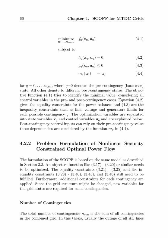
66 Chapter 4. SCOPF for MTDC Grids
minimizeu0,...,uncon
f0(x0,u0) (4.1)
subject to
hq(xq,uq) = 0 (4.2)
gq(xq,uq) ≤ 0 (4.3)
mq(u0) = uq (4.4)
for q = 0, . . . , ncon, where q=0 denotes the pre-contingency (base case)state. All other denote to different post-contingency states. The objec-tive function (4.1) tries to identify the minimal value, considering allcontrol variables in the pre- and post-contingency cases. Equation (4.2)gives the equality constraints for the power balances and (4.3) are theinequality constraints such as line, voltage and generators limits foreach possible contingency q. The optimization variables are separatedinto state variables xq and control variables uq and are explained below.Post-contingency control inputs can rely on their pre-contingency valuethese dependencies are considered by the function mq in (4.4).
4.2.2 Problem Formulation of Nonlinear SecurityConstrained Optimal Power Flow
The formulation of the SCOPF is based on the same model as describedin Section 3.3. An objective function like (3.17) - (3.20) or similar needsto be optimized. The equality constraints (3.21) - (3.25) and the in-equality constraints (3.28) - (3.40), (3.45), and (3.46) still need to befulfilled. Furthermore, additional constraints for each contingency areapplied. Since the grid structure might be changed, new variables forthe grid states are required for some contingencies.
Number of Contingencies
The total number of contingencies ncon is the sum of all contingenciesin the combined grid. In this thesis, usually the outage of all AC lines

4.2. Nonlinear SCOPF for Combined AC and DC Grids 67
(including the transformers) and DC lines are considered. Also all gen-erators, either in the AC or DC grid can fail, and each converter canhave an outage.
ncon = nACcon,lin + nDC
con,lin + nACcon,gen + nDC
con,gen + ncon,vsc (4.5)
In a meshed transmission grid nACcon,lin is equal to nAC
lin , since each linecan have a contingency. If the topology includes radial connections, theycannot be included in the N-1 criterion. Therefore the above statedequation changes to nAC
con,lin ≤ nAClin . The same is valid for the DC lines.
Generators and converters are only excluded from the N-1 criterion, ifthey are the only source for a load. This barely happens in a transmissiongrid. Of course the whole grid cannot be entitled as N-1 secure in sucha case.
4.2.3 Problem Formulation of Nonlinear SecurityConstrained Optimal Power Flow with Pre-ventive Control
If the preventive SCOPF control is applied for all line and generatorcontingencies, the DC converter power flows are kept constant. Thishas the effect that the converters are controllable barriers for the faults.If asynchronous grids are coupled, then each grid has to handle its ownproblems. The spreading of a fault can be contained. This behavior couldprevent the spread of a fault, but also limits the flexibility introducedby the converters.
Each contingency is modeled by considering the same equality and in-equality constraints as for the base problem and adding them up. De-pending on the contingency, different changes need to be done to theadded equations and inequalities.
State and Control Variables
The vector zq consists of the state variables xq and the control vari-ables uq. All possible variables in the state and control vector for thepreventive case are given as follows:

68 Chapter 4. SCOPF for MTDC Grids
zq =
xq
uq
(4.6)
xq =
x0
uACq
θq
uDCq
(4.7)
uq =
u0
pACcon,slack
qcon
(4.8)
As explained below, not each contingency requires the same amount ofadditional states and control variables in the preventive case, e.g. anAC line outage needs no changes in the DC grid. An overview of therequired variables is given in Table 4.1.
Objective Function
The objective function is still the same as in (3.16)–(3.20), since the costis based only on the nominal (base case) states. It would also be possible
Table 4.1: Additional variables for each contingency for preventivecontrol cases.
Contingency uACk,q θk,q uDC
i,q pACc,q,slack qc,q
AC line Yes Yes No No NoDC line No No Yes No NoGenerator AC grid Yes Yes No No NoGenerator DC grid No No Yes No NoConverter station Yes Yes Yes Yes Yes

4.2. Nonlinear SCOPF for Combined AC and DC Grids 69
to optimize the differences between the pre- and post-contingency states,which is not done here.
Equality Constraints
The equality constraints for the preventive controlled SCOPF are thesame as (3.22)–(3.25). Each constraint has to be fulfilled for each con-tingency case. This increases the problem size significantly.
Inequality Constraints
In general, the inequality constraints from the nominal case are validfor each contingency, but since only some variables change, not all areneeded to ensure an operation within the limits.
AC Line Outages from k to m changes the contingency problemby removing one flow equation of the kind (3.1) and (3.2). The newflows require new system states, therefore the state vector xq, whereq is equal to the number of the AC line contingency, contains the newvoltage magnitude uAC
q and voltage angles θkm,q. The generated activepower, the converter powers and the flow in the DC grid stay withinthe nominal values.
All equality constraints have to be fulfilled with the new variables. Alsothe inequality constraints add new equation in this case.
sACmin,km ≤ sAC
q,km ≤ sACmax,km (4.9)
sACmin,mk ≤ sAC
q,mk ≤ sACmax,mk (4.10)
uACmin,k ≤ uAC
q,k ≤ uACmax,k (4.11)
DC Line Outages from i to j change only the flows in the DC grid forthe preventive controlled SCOPF. Also in that case, additional statesin the DC grid are required, the contingency case voltages uDC
q arealso added to the state vector xq. In this case the generated power,the converter powers and the flows in the AC grid stay at the nominal
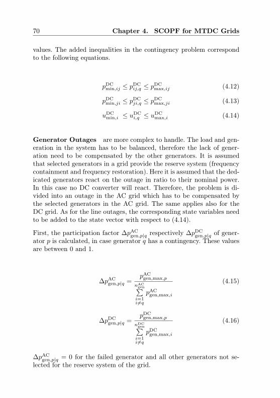
70 Chapter 4. SCOPF for MTDC Grids
values. The added inequalities in the contingency problem correspondto the following equations.
pDCmin,ij ≤ pDC
ij,q ≤ pDCmax,ij (4.12)
pDCmin,ji ≤ pDC
ji,q ≤ pDCmax,ji (4.13)
uDCmin,i ≤ uDC
i,q ≤ uDCmax,i (4.14)
Generator Outages are more complex to handle. The load and gen-eration in the system has to be balanced, therefore the lack of gener-ation need to be compensated by the other generators. It is assumedthat selected generators in a grid provide the reserve system (frequencycontainment and frequency restoration). Here it is assumed that the ded-icated generators react on the outage in ratio to their nominal power.In this case no DC converter will react. Therefore, the problem is di-vided into an outage in the AC grid which has to be compensated bythe selected generators in the AC grid. The same applies also for theDC grid. As for the line outages, the corresponding state variables needto be added to the state vector with respect to (4.14).
First, the participation factor ∆pACgen,p|q respectively ∆pDC
gen,p|q of gener-ator p is calculated, in case generator q has a contingency. These valuesare between 0 and 1.
∆pACgen,p|q =
pACgen,max,p
nACgen∑i=1i6=q
pACgen,max,i
(4.15)
∆pDCgen,p|q =
pDCgen,max,p
nDCgen∑i=1i6=q
pDCgen,max,i
(4.16)
∆pACgen,p|q = 0 for the failed generator and all other generators not se-
lected for the reserve system of the grid.
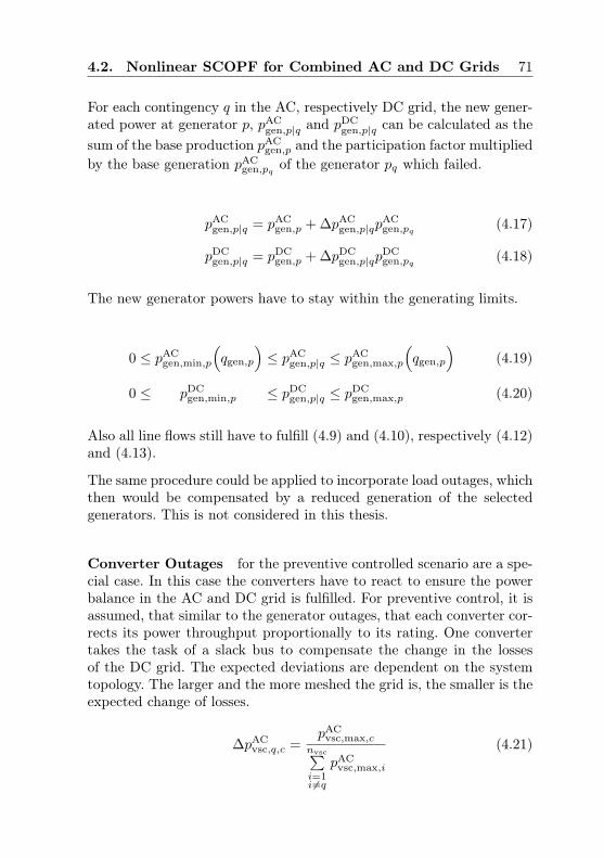
4.2. Nonlinear SCOPF for Combined AC and DC Grids 71
For each contingency q in the AC, respectively DC grid, the new gener-ated power at generator p, pAC
gen,p|q and pDCgen,p|q can be calculated as the
sum of the base production pACgen,p and the participation factor multiplied
by the base generation pACgen,pq of the generator pq which failed.
pACgen,p|q = pAC
gen,p + ∆pACgen,p|qp
ACgen,pq (4.17)
pDCgen,p|q = pDC
gen,p + ∆pDCgen,p|qp
DCgen,pq (4.18)
The new generator powers have to stay within the generating limits.
0 ≤ pACgen,min,p
(qgen,p
)≤ pAC
gen,p|q ≤ pACgen,max,p
(qgen,p
)(4.19)
0 ≤ pDCgen,min,p ≤ pDC
gen,p|q ≤ pDCgen,max,p (4.20)
Also all line flows still have to fulfill (4.9) and (4.10), respectively (4.12)and (4.13).
The same procedure could be applied to incorporate load outages, whichthen would be compensated by a reduced generation of the selectedgenerators. This is not considered in this thesis.
Converter Outages for the preventive controlled scenario are a spe-cial case. In this case the converters have to react to ensure the powerbalance in the AC and DC grid is fulfilled. For preventive control, it isassumed, that similar to the generator outages, that each converter cor-rects its power throughput proportionally to its rating. One convertertakes the task of a slack bus to compensate the change in the lossesof the DC grid. The expected deviations are dependent on the systemtopology. The larger and the more meshed the grid is, the smaller is theexpected change of losses.
∆pACvsc,q,c =
pACvsc,max,c
nvsc∑i=1i6=q
pACvsc,max,i
(4.21)

72 Chapter 4. SCOPF for MTDC Grids
The new power flow for converter c in case q is a converter contingencycan be calculated by the sum of the base flow pAC
vsc,c and the participationfactor ∆pAC
vsc,c multiplied with the base case power flow in the convertercq, which has the outage.
pACvsc,q,c = pAC
vsc,c + ∆pACvsc,q,cp
ACvsc,cq (4.22)
and has to stay within the given limits.
pACvsc,min,c
(qvsc,c
)≤ pAC
vsc,q,c ≤ pACvsc,max,c
(qvsc,c
)(4.23)
The outage of a converter station changes the flows in the AC and DCgrid. Therefore, these outages require additional state variables in bothgrids.
4.2.4 Problem Formulation of Nonlinear SecurityConstrained Optimal Power with CorrectiveControl
This formulation uses the fast controllable VSC to influence the powerflows after a contingency in the grid. This method has no fault ridethrough barriers. This means every contingency in one grid will influencethe other grid parts or connected asynchronous areas. This behaviormakes also the distinction between contingencies in either the AC or DCgrid unnecessary. Since the converters can react for each contingency, anew set of state and decision variable is required.
State and Control Variables
The vector zq consists out of the state variables xq and the controlvariables uq. All possible variables in the state and control vector forthe corrective case are given as follows:

4.2. Nonlinear SCOPF for Combined AC and DC Grids 73
zq =
xq
uq
(4.24)
xq =
x0
uACq
θq
uDCq
(4.25)
uq =
u0
pACvsc,q
qvsc,q
(4.26)
The expanded optimization variable vector zq looks similar to (4.6),but the converter flow variable pAC
vsc,q,c is different, which changes theoptimization significantly. Therefore, for each contingency a full set ofvariables need to be added which significantly increases the amount ofvariables. This is described in Table 4.2.
Table 4.2: Additional variables for each contingency for corrective con-trol case.
Contingency uACq,k θq,k uDC
q,i pACvsc,q,c qvsc,q,c
AC Line Yes Yes Yes Yes YesDC line Yes Yes Yes Yes YesGenerator AC grid Yes Yes Yes Yes YesGenerator DC grid Yes Yes Yes Yes YesConverter station Yes Yes Yes Yes Yes

74 Chapter 4. SCOPF for MTDC Grids
Objective Function
The objective function is still the same as in (3.16)–(3.20). Here it couldmake sense to consider the following additional term to the objectivefunction:
fvsc(x,u) = π
nvsc∑c=1
(pACvsc,c − pAC
vsc,q,c
)2
(4.27)
Equation (4.27) penalizes the difference between the flows before andafter a contingency through the converters. This will limit the changesand introduces some failure barriers. There is a trade-off between thecost for solving the problem within the own grid and spreading it to theother parts. The factor π is a scaling factor, which is useful to define theweight of this term if it is added to any of the other objective functions.
Equality Constraints
The equality constraints for each contingency are based on (3.22)–(3.25).The new converter transfer power pAC
vsc,q,c has to be used for each con-tingency.
Inequality Constraints
The same is valid for the inequality constraints. For each contingency aset like (3.28)–(3.46) is added to the problem formulation.
If the pre- and post-contingency deviation in the converter should notonly be penalized in the optimization function, thus a strict limit ispossible.
|pACvsc,c − pAC
vsc,q,c| ≤ ∆pACvsc,max,c (4.28)
where ∆pACvsc,max,c gives a fixed limit for each converter c, how much
its post-contingency value is allowed to vary from the pre-contingencystate.
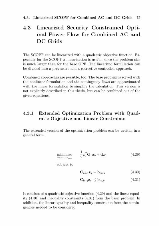
4.3. Linearized SCOPF for Combined AC and DC Grids 75
4.3 Linearized Security Constrained Opti-mal Power Flow for Combined AC andDC Grids
The SCOPF can be linearized with a quadratic objective function. Es-pecially for the SCOPF a linearization is useful, since the problem sizeis much larger than for the base OPF. The linearized formulation canbe divided into a preventive and a corrective controlled approach.
Combined approaches are possible, too. The base problem is solved withthe nonlinear formulation and the contingency flows are approximatedwith the linear formulation to simplify the calculation. This version isnot explicitly described in this thesis, but can be combined out of thegiven equations.
4.3.1 Extended Optimization Problem with Quad-ratic Objective and Linear Constraints
The extended version of the optimization problem can be written in ageneral form.
minimizeu0,...,uncon
1
2zT
0 G z0 + dz0 (4.29)
subject to
Ceq,qzq = beq,q (4.30)
Ciq,qzq ≤ biq,q (4.31)
It consists of a quadratic objective function (4.29) and the linear equal-ity (4.30) and inequality constraints (4.31) from the basic problem. Inaddition, the linear equality and inequality constraints from the contin-gencies needed to be considered.

76 Chapter 4. SCOPF for MTDC Grids
4.3.2 Problem Formulation of Linear Security Con-strained Optimal Power Flow Preventive Con-trol
The details about the problem formulation in (4.29) to (4.31) are ex-plained below.
State and Control Variables
All additional required security margins can be calculated from the nom-inal linearized optimization vector z from (3.63), therefore no changesin the vector z are required and zq = z holds for this formulation.
Objective Function
The objective function still needs to define the allocation of power flowsbetween the AC and DC grid. Therefore (3.69) is still valid as the objec-tive function which penalizes the flows according to their caused lossesin the grids and converters.
Equality Constraints
The equality constraints are the AC bus power balances (3.73) and thesame for the DC buses (3.74). The matrix formulation (3.75)–(3.77) canbe used here as well.
Inequality Constraints
The major changes are applied to the inequality constraints. The knownconcepts of line outage distribution factor (LODF) and generalized gen-eration distribution factors (GGDF), explained in [80], are expanded toinclude DC lines and converter outages.

4.3. Linearized SCOPF for Combined AC and DC Grids 77
AC Line Contingencies from k to m are considered with LODF.They are defined in (4.32) for each line km in any possible outage ofanother line vw.
LODFACkm,vw =
∆pACkm
pACvw,0
(4.32)
where ∆pACkm is the change in flow on line km and pAC
vw 0 is the flow online from v to w before the contingency occurred. The exact derivationof the LODF can be found in [80]. They can be calculated directly fromthe system parameters.
DC Line Contingencies from i to j use a similar principle as in theAC grid, since the linearized formulations have the same structure. Thedirect current line outage distribution factors (DCLODFs) are derivedbelow. The contingency of a DC line is compensated as the additionalinjection of the line power flow at the incident nodes. Figure 4.1 showsthe modeling of the pre- and post-contingency situation. This resultsin an incremental change ∆uDC. It is assumed that all converters arein power control mode. Only one converter is controlling the voltage inthe DC grid. A voltage change at this converter changes the referencevalue and all voltages have to be adjusted.
The relationship between the change in the power injections ∆p and thevoltages are described by the Z matrix.
∆uDC = Z∆pDC (4.33)
For a line outage from node i to j we have:
∆pDC = [0 . . . ∆ui . . . 0 . . . ∆uj . . . 0]T (4.34)
where ∆ui = −∆uj , due to the lossless formulation.

78 Chapter 4. SCOPF for MTDC Grids
DC bus i DC bus j
uDCi uDC
j
pDCij
Connectionto otherDC buses
Connectionto otherDC buses
(a)
DC bus i DC bus j
uDCi uDC
j
pDCij
Connectionto otherDC buses
Connectionto otherDC buses
∆pi ∆pj
(b)
Figure 4.1: Pre- and post-contingency DC lines faults situation. (a)The standard situation of the DC grid without any contin-gency. (b) The modeled situation after a DC line outage,the line outage is compensated by power injections on theend of the line.
The voltage changes can be described as follows:
∆uDCi =(Zii − Zij
)∆pi (4.35)
∆uDCj =(− Zjj + Zij
)∆pi (4.36)
The new flows over the tripped line pDCij can be calculated from the
original flow pDCij and the change in the flow ∆pij .
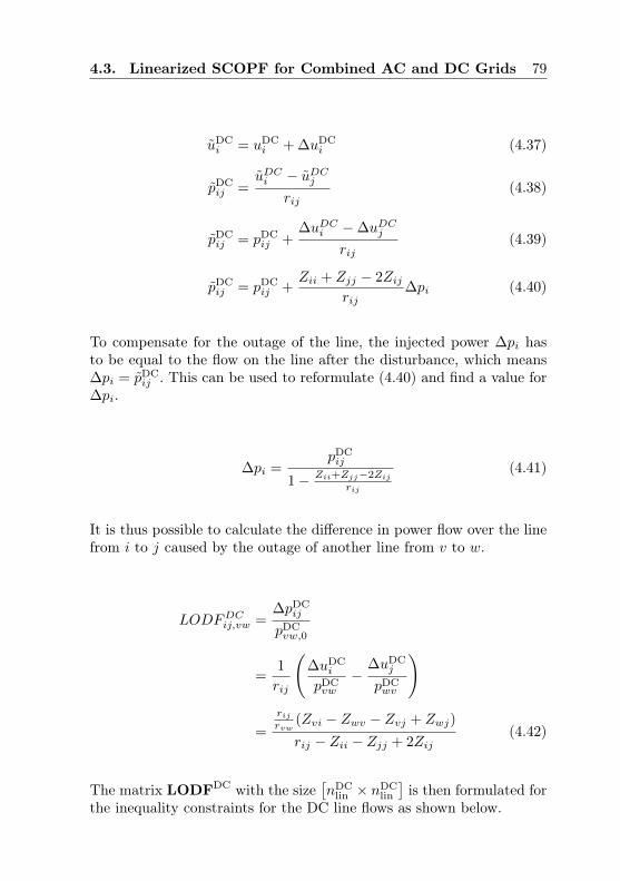
4.3. Linearized SCOPF for Combined AC and DC Grids 79
uDCi = uDC
i + ∆uDCi (4.37)
pDCij =
uDCi − uDCjrij
(4.38)
pDCij = pDC
ij +∆uDCi −∆uDCj
rij(4.39)
pDCij = pDC
ij +Zii + Zjj − 2Zij
rij∆pi (4.40)
To compensate for the outage of the line, the injected power ∆pi hasto be equal to the flow on the line after the disturbance, which means∆pi = pDC
ij . This can be used to reformulate (4.40) and find a value for∆pi.
∆pi =pDCij
1− Zii+Zjj−2Zij
rij
(4.41)
It is thus possible to calculate the difference in power flow over the linefrom i to j caused by the outage of another line from v to w.
LODFDCij,vw =∆pDC
ij
pDCvw,0
=1
rij
(∆uDC
i
pDCvw
−∆uDC
j
pDCwv
)
=
rijrvw
(Zvi − Zwv − Zvj + Zwj)
rij − Zii − Zjj + 2Zij(4.42)
The matrix LODFDC with the size[nDC
lin × nDClin]is then formulated for
the inequality constraints for the DC line flows as shown below.

80 Chapter 4. SCOPF for MTDC Grids
Generator Contingencies in the AC grid are considered by usingthe GGDF factors [80]. They are defined as:
GGDFACkm,p =
∆pACkm
∆pp(4.43)
∆pi is defined as the change in generation at generator p. The outage ofa generator is compensated by all controllable generators proportionalto their maximum power, given as rAC
gen.
Generator Contingencies in the DC grid are considered byusing the direct current generalized generation distribution factor(DCGGDF). Equation (4.33) is used as the base for their calculation.The difference compared to the LODF is the definition of ∆p. A gen-eration loss of one unit (-1 p.u.) is used to indicate the outage of agenerator q. All the other controllable generators compensate the lossof generation proportional to their maximal capacity. The assumptionis made that there is more than one generator in the DC grid, otherwisethe DC grid cannot handle the generator contingency by itself. Only thecorrective controlled case could handle such a case, which is explainedin the next section.
∆pq,p = −pgen,p,max
nDCgen∑p=1p6=q
pgen,p
· (−1) (4.44)
This gives ∆pq as follows.

4.3. Linearized SCOPF for Combined AC and DC Grids 81
∆pq = rDCgen =
∆p1
∆p2
...
−1
...
∆pnDCgen
qth row
(4.45)
The influence on DC line ij in case of an outage of generator q can thenbe calculated.
GGDFDCij,q =
∆pij∆pq
=1
rij
(∆uDC
i
∆pq−
∆uDCj
∆pp
)
=Ziq − Zjq
rij(4.46)
The matrix GGDFDC with the size[nDC
lin × nDCgen]is then used for en-
suring the DC line flow constraints as in case of a generator outageas shown below. The generator outputs have to stay within the limitsincluding the changes applied during a contingency, as shown later.
Converter Contingencies are considered by using converter outagedistribution factor (CODF). They are calculated similarly to the GGDF.They are defined as a factor about how much of the converter transferpower is shifted to an AC or DC line in case of the outage of a con-verter station. In such a case, it is assumed that the remaining converterstations take over the power proportionally to their maximal capacitypower. This results in a similar solution, as the idea of a decentralizedcontrol structure of sharing the power deviation of a disturbance in theDC grid by adjusting the voltages. The outage of a converter stationleads to new flows in the AC and DC grid.

82 Chapter 4. SCOPF for MTDC Grids
∆pvsc,q,c = − pvsc,cnvsc∑i=1i6=q
pvsc,max,c
· (−1) (4.47)
The readjusted power setpoints compensate completely the contingencyin one converter, since the losses are neglected in this approach and thereis no need for a slack converter. The same steps as for (4.45) and (4.46)lead to the solution for the outage of converter r.
CODFDCij,r =
∆pDCij
∆pDCr
=1
rij
(∆uDC
i
∆pDCr
−∆uDC
j
∆pDCr
)
=Zir − Zjq
rij(4.48)
If the converter power flows are changed, not only the DC side is af-fected, but also the AC side. The CODF on the AC side are calculatedanalogous to the GGDF.
CODFACkm,r =∆pAC
km
∆pACr
=1
zkm
(∆θkdpACp
− ∆θm∆pAC
r
)
=Xkp −Xmp
zkm(4.49)
where
∆θ = X∆pACvsc (4.50)
Equation (4.48) is similar to (4.46), since a failure of a converter stationhas a similar impact in the grid as an outage of a generator or load

4.3. Linearized SCOPF for Combined AC and DC Grids 83
which is tackled as a constant negative generator. The difference is thatfor a generator outage all other generators have to ramp up their poweroutput. When a converter has an outage, the changes in the power setpoint can be positive or negative, depending on the actual power in theconverter.
The formulated factors LODF, GGDF, rgen, CODF, and rvsc can nowbe used to formulate all linear inequality constraints for the SCOPF.I is the identity matrix of appropriate dimensions.
pgen,min ≤(I + rgen
)pgen ≤ pgen,max (4.51)
pvsc,min ≤(I + rvsc
)pvsc ≤ pvsc,max (4.52)
pACmin ≤
(I + LODFAC
)BACθ ≤ pAC
max (4.53)
pACmin ≤ BACθ + GGDFACpAC
gen ≤ pACmax (4.54)
pACmin ≤ BACθ + CODFACpvsc ≤ pAC
max (4.55)
pDCmin ≤
(I + LODFDC
)BDCuDC ≤ pDC
max (4.56)
pDCmin ≤ BDCuDC + GGDFDCpDC
gen ≤ pDCmax (4.57)
pDCmin ≤ BDCuDC + CODFDCpvsc ≤ pDC
max (4.58)
Inequality (4.51) constrains the generators, which have to stay withintheir limits by adding the nominal production to the reserves for cov-ering generator outages. The same is valid for the converters in (4.52).The next three inequalities limit the flows on the AC lines. Consider-ing other AC line outages with (4.53), followed by the line limits forgenerator outages (4.54), and converter outages (4.55). The last threeinequalities (4.56)–(4.58) ensure the limits for the DC lines and also forline, generator, and converter contingencies.

84 Chapter 4. SCOPF for MTDC Grids
4.3.3 Problem Formulation of Linear Security Con-strained Optimal Power Flow with CorrectiveControl
The implementation of corrective control into the linearized version re-sults in a more complex formulation. This still has a quadratic objec-tive function and linearized constraints, but additional variables andconstraints are required. The basic assumption is as in the nonlinearcase, that the controllable devices are the converter stations. The gen-erators react only on power imbalances in the grid, which correspond togenerator outages.
State and Control Variables
Each contingency requires a new set of variables for the converter powerflows. This allows an adjusted power setpoint for the new grid situationwhich could lead to a significant change in power flows in both gridsand also requires new state variables for voltage angles in the AC gridand voltage deviations in the DC grid.
zq =
z
θq
uDCq
pvsc,q
(4.59)
The number of variables can be calculated by taking the number ofvariables for the base case and multiply the new variables by the numberof contingencies.
nz = ngen + nACbus + nDC
bus + nvsc + ncon
(nAC
bus + nDCbus + nvsc
)= ngen +
(ncon + 1
)(nAC
bus + nDCbus + nvsc
)(4.60)

4.3. Linearized SCOPF for Combined AC and DC Grids 85
Objective Function
The objective function has to overcome the same challenges, as in thebasic linearized OPF. Therefore (3.69) is still valid as the objectivefunction, which penalizes the flows according to their caused estimatedlosses in the grids and converters.
Equality Constraints
Each contingency adds a set of matrices according to (3.75) to the equal-ity constraints. Depending on the contingency the corresponding matri-ces BAC, HAC, T, HDC, S or BDC needed to be adjusted. In case ofa converter outage T and S are changed at the same time. The corre-sponding state vector xq is used and beq,q is reduced by the affectedvalue of the contingency.
Inequality Constraints
The inequality constraints for the corrective control are also dependenton the individual contingency. Each contingency adds a similar set ofinequalities Ceq,q as defined in (3.85), with the corresponding new vari-ables. For all contingencies the generators do not change their poweroutput, thus rows 5 and 6 are removed from (3.86). For line outages inthe AC grid, AAC is adjusted. The same happens for ADC if a line in theDC grid has a contingency. The matrix Invsc ensures that the new powersetpoints for the converters are within the allowed limits. The matrixneeds to be changed only in case of a converter outage. In that case thecorresponding row has to be removed. The matrix L stays the same foreach contingency, since complete bus outages are not considered.
To limit the fault ride through behavior, the limitation of the converterdeviation between pre- and post-contingency states can also be limited,as descried in (4.28).
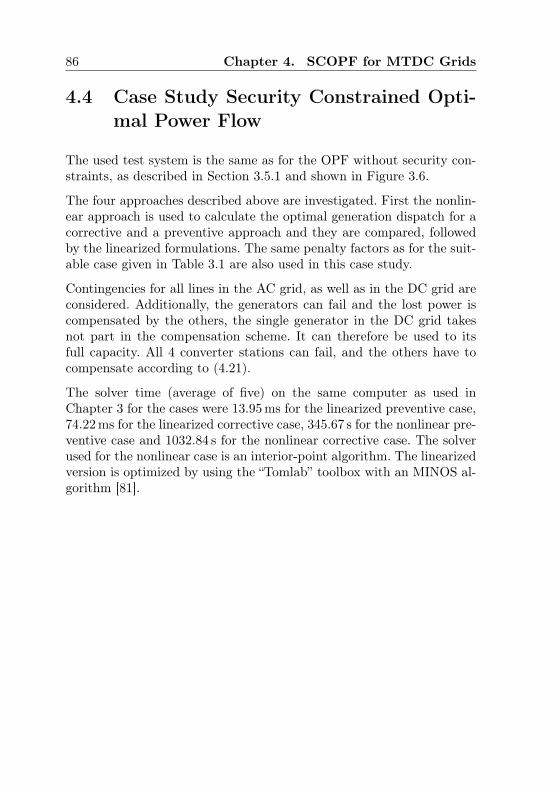
86 Chapter 4. SCOPF for MTDC Grids
4.4 Case Study Security Constrained Opti-mal Power Flow
The used test system is the same as for the OPF without security con-straints, as described in Section 3.5.1 and shown in Figure 3.6.
The four approaches described above are investigated. First the nonlin-ear approach is used to calculate the optimal generation dispatch for acorrective and a preventive approach and they are compared, followedby the linearized formulations. The same penalty factors as for the suit-able case given in Table 3.1 are also used in this case study.
Contingencies for all lines in the AC grid, as well as in the DC grid areconsidered. Additionally, the generators can fail and the lost power iscompensated by the others, the single generator in the DC grid takesnot part in the compensation scheme. It can therefore be used to itsfull capacity. All 4 converter stations can fail, and the others have tocompensate according to (4.21).
The solver time (average of five) on the same computer as used inChapter 3 for the cases were 13.95 ms for the linearized preventive case,74.22 ms for the linearized corrective case, 345.67 s for the nonlinear pre-ventive case and 1032.84 s for the nonlinear corrective case. The solverused for the nonlinear case is an interior-point algorithm. The linearizedversion is optimized by using the “Tomlab” toolbox with an MINOS al-gorithm [81].

4.4. Case Study Security Constrained OPF 87
4.4.1 Results
Costs
The costs in the different cases are shown in Figure 4.2. The nonlinearSCOPF with corrective control has cost which is 11.7 % lower thanthe nonlinear preventive case. This difference shows the value of theflexibility of the converter stations which can react after a contingency.
The linearized cases show both a similar behavior as their nonlinearequivalent. The generation cost is lower, since the losses are not con-sidered in this case. The total objective function values, including thepenalty terms, marked with the striped areas, give almost the same costas in the nonlinear case. There is a deviation of 1.7 % in the correctivecase and 1.5 % in the preventive case.
40.0
42.5
45.0
47.5
50.0
52.5
55.0
57.5
Cos
t(m
.u.)
Nonlin SCOPF Corrective Nonlin SCOPF PreventiveLinear SCOPF Corrective Linear SCOPF Preventive
Figure 4.2: Comparison of costs in m.u. for the nonlinear correc-tive, preventive and linearized corrective and preventiveSCOPF, in the IEEE14 bus test grid, with an addedMTDC system. The filled areas correspond to the gen-eration costs, and the striped area represent the penaltyterms.
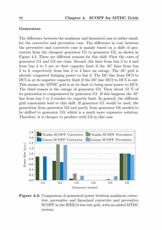
88 Chapter 4. SCOPF for MTDC Grids
Generators
The difference between the nonlinear and linearized case is rather small,for the corrective and preventive case. The difference in cost betweenthe preventive and corrective case is mainly based on a shift of gen-eration from the cheapest generator G1 to generator G2, as shown inFigure 4.3. There are different reasons for this shift. First the costs ofgenerator G1 and G2 are close. Second, the lines from bus 3 to 4 andfrom bus 4 to 5 are at their capacity limit if the AC lines from bus2 to 3, respectively from bus 2 to 4 have an outage. The AC grid isalready congested bringing power to bus 3. The DC line from DC3 toDC5 is at its negative capacity limit if the DC line DC2 to DC5 is out.This means the MTDC grid is at its limit to bring more power to DC3.The third reason is the outage of generator G2. Then about 52 % ofits generation is compensated by generator G1. If this happens the ACline from bus 1 to 2 reaches its capacity limit. In general, the differentgrid constraints lead to this shift. If generator G1 would be used, thegeneration from generator G2 and partly from generator G6 needed tobe shifted to generator G3, which is a much more expensive solution.Therefore, it is cheaper to produce with G2 in this case.
G1 G2 G3 G4 G5 G60.0
0.2
0.4
0.6
0.8
1.0
1.2
1.4
1.6
1.8
Generator number
Pow
erflo
w(p.u.)
Nonlin SCOPF Corrective Nonlin SCOPF PreventiveLinear SCOPF Corrective Linear SCOPF Preventive
Figure 4.3: Comparison of generated power between nonlinear correc-tive, preventive and linearized corrective and preventiveSCOPF in the IEEE14 bus test grid, with an added MTDCsystem.

4.4. Case Study Security Constrained OPF 89
Converters
The same behavior as for the generators is seen for the converters asshown in Figure 4.4. Since there is almost no generation at generatorG1, the converter C1 connected to bus 1 is reduced from 34.38 MW inthe linearized corrective case to 4.45 MW in the preventive case. Onthe other side the power at converter C3 is reduced significantly. Thisshows a limitation of the preventive control operation if it is applied toa rather small MTDC system.
Another effect is the remarkable difference between the nonlinear andthe linearized flow for converter C2 and C3. In sum there are more orless equal, but the allocation is different. The nonlinear corrective caseuses almost only converter C2 and the transports the power throughthe AC grid. The linearized version distributes the flow to C2 and C3.
C1 C2 C3 C4−0.6
−0.4
−0.2
0.0
0.2
0.4
0.6
0.8
Converter number
Con
vert
erpo
wer
(p.u
.)
Nonlin SCOPF Corrective Nonlin SCOPF PreventiveLinear SCOPF Corrective Linear SCOPF Preventive
Figure 4.4: Comparison of the power flow through the four convert-ers between nonlinear corrective, preventive and linearizedcorrective and preventive SCOPF in the IEEE14 bus testgrid, with an added MTDC system.

90 Chapter 4. SCOPF for MTDC Grids
AC and DC Transmission Lines
The line flows follow the converter powers as shown in Figure 4.5. Thecorrective case shows two general flow directions: one from C1 to C4and another from DC5 to all the other converters. The preventive casechanges this pattern. The infeed happens only at DC5 and flows to theother DC buses. There is also a flow from DC5 to DC1 and further toDC4. This also leads to power reversals in three lines. The overall usageis reduced and the lines are not used heavily, which gives another hintof the underutilization with the preventive case.
In order to complete the explanations above Figure 4.6 shows the flowsin all 20 AC lines. Obviously line 1 has a large difference between thecorrective and preventive flow for the same reasons as explained above.
DC1-D
C4
DC1-D
C5
DC2-D
C3
DC2-D
C5
DC3-D
C4
DC3-D
C5
DC4-D
C5−0.6
−0.4
−0.2
0.0
0.2
0.4
0.6
0.8
DC line from bus to bus
Pow
erflo
w(p.u.)
Nonlin SCOPF Corrective Nonlin SCOPF PreventiveLinear SCOPF Corrective Linear SCOPF Preventive
Figure 4.5: Comparison of power flow through seven DC lines betweennonlinear corrective, preventive and linearized correctiveand preventive SCOPF in the IEEE14 bus test grid, withan added MTDC system.

4.4. Case Study Security Constrained OPF 91
1 2 3 4 5 6 7 8 9 10 11 12 13 14 15 16 17 18 19 20
−0.3
−0.2
−0.1
0.0
0.1
0.2
0.3
0.4
0.5
0.6
AC line number
Pow
erflo
w(p.u.)
Nonlin SCOPF Corrective Nonlin SCOPF PreventiveLinear SCOPF Corrective Linear SCOPF Preventive
Figure 4.6: Comparison of power flow through 20 AC lines betweennonlinear corrective, preventive and linearized correctiveand preventive SCOPF in the IEEE14 bus test grid, withan added MTDC system.

92 Chapter 4. SCOPF for MTDC Grids
4.5 Conclusion
The SCOPF problem is extended in this chapter to also incorporate DCgrids. This provides the basic requirements for all TSOs to operate afuture grid which includes combined AC and DC grids.
Two different calculation methods combined with two different controlmethods are investigated. The nonlinear calculations are used to givea calculation as accurate as possible, with the drawback of increasedcomputational effort. To avoid this, the linearized version is given, whichapproximates the flows with linear equations.
The preventive control method sets the values of the converter flows be-fore the contingency happens. They are not allowed to react afterwards.This will limit the flexibility and blocks the expansion of a disturbancethrough the DC grid. In the corrective case, the converters are allowed toreact after a contingency and can correct their setpoints. This increasesthe flexibility, but disturbances are spread throughout both grids.
For the linearized case the concept of DCLODF is derived, which issimilar to the LODF in the AC grid. In addition, the CODFs are intro-duced, to show the influence of a converter outage to the AC line powerflows and DC line power flows.
The case study shows that the linearized method works well for theSCOPF. Additionally, it shows the limitation of the preventive con-trolled method. Whereby the flexibility of the MTDC is limited as ithas to handle outages within the DC grid by its own.
The value of this flexibility and some sensitivity analysis are shown ina more detailed study in the next chapter.

Chapter 5
Case Study and SensitivityAnalyses
This chapter presents different simulation studies. A smaller 14 bus sys-tem and a larger 73 bus system are used to perform calculations basedon the formulations described in Chapter 3 and 4. Additionally, the sen-sitivity of the solutions regarding different grid parameters is assessed.
5.1 Test Setup
This chapter is based on two different test grids. It starts by definingthe topologies and parameters of these grids. The details of both gridare given in Appendix C.
5.1.1 Study Grid Topology
Smaller Grid
The smaller grid is the IEEE14 bus power flow test case which hasalready been used in the previous chapters. It is shown in Figure 3.2.The 14 bus AC grid is expanded by a meshed five bus MTDC overlaygrid. There are five generators in the AC grid and one in the DC grid.
93

94 Chapter 5. Case Study and Sensitivity Analyses
Larger Grid
The larger grid is given in Figure 5.1. This grid is based on the ReliabilityTest System 1996 (RTS96) [82], available in [83]. Three similar areasare coupled with tie lines. The total system consists of 73 AC busesconnected with 120 AC lines. The MTDC grid, consists of eight DCbuses connected with 16 DC transmission lines. It is constructed toconnect the northern and southern part in each area and increases thetransmission capacity between the areas. The MTDC grid has two buseswith no connection to the AC grid. Buses 7 and 8 are the connectionpoints for cheap generators, which could represent e.g. wind parks. Theydo not participate in the power balancing process.
5.1.2 Test Cases
For both grids the base loads are multiplied by a load factor sload,to show the effect of the MTDC grid for different stress levels of thecombined grid.
p′load,k = sload pload,k k = 1, . . . , nACbus (5.1)
The chosen values for sload are 0.9, 1.0, 1.1 and 1.2.
Smaller Grid For the small grid the same parameters as explainedin Section 3.5.1 are used. They are based on the original values given in[84]. All other parameters are defined in Tables C.1 to C.5.
Large Grid The AC part of the large grid uses data available in[83]. The original grid has large security margins, and so there is noneed for a grid extension. Therefore, the transmission capacity betweenthe northern and southern part of the grid was reduced by 15 %. Thedetailed data is available in Table C.7. Table C.8 describes the converterparameters and Table C.9 gives the parameters of the 16 DC lines.

5.1. Test Setup 95
101
102
103 10
4
105
106
107
108
109
110
111
112
113
114
115
116
117
118
119
120
121
122
123
124
201
202
203 20
4
205
206
207
208
209
210
211
212
213
214
215
216
217
218
219
220
221
222
223
224
301
302
303 30
4
305
306
307
308
309
310
311
312
313
314
315
316
317
318
319
320
321
322
323
324
325
DC
1
DC
2
DC
3
DC
4
DC
5
DC
6D
C7
DC
8
AC
Bus
AC
Line
DC
Bus
DC
Line
Gen
erat
orLo
adTra
nsfo
rmer
VSC
Figure
5.1:
Larger
test
grid,b
ased
onthreearea
RTS9
6test
grid
(black)expa
nded
withan
eigh
tbu
sMTDC
overlaygrid
(green).

96 Chapter 5. Case Study and Sensitivity Analyses
To have inter-area flows, the base loads in Area 1 are increased by 10 %.In Area 2 the base load is decreased by the same amount. The base loadin Area 3 is not modified. The generator costs are taken from [85] andgiven in Table C.10.
If nothing else is indicated all simulations are processed by using thelinearized OPF or SCOPF. As shown in the previous chapters they givea good accuracy and guarantee a global optimum solution.
5.2 Results
The grid described above where used to perform different analyses withthe algorithms. A comparison of the cost and the sensitivity of the pricesdepending on how converter flexibility is implemented. Additionally, theconverter and DC line capacities are investigated.
5.2.1 Costs
The generation cost given in normalized m.u., including the penaltyterms for different operation principles are given in Figure 5.2 for thesmall grid and in Figure 5.4 for the large grid respectively. The base forthe normalization are the cost for the grid without an MTDC grid, ifno security assessments are applied (dark green bar).
Smaller grid
The first two bars show the operating cost with only the existing ACgrid, with and without security measures to counteract contingencies.The differences in costs are with 14.83 % quite significant, since theintroduction of the N-1 criterion leads to a shift of the generation fromthe cheapest generator G1 to the others in the grid. These points aregiven to have a reference value of the relative increase caused by addedsecurity measures. The absolute value of the cost is not directly compa-rable to the operating cost including an MTDC grid, due to the needof additional investment. This could also be done by adding AC lines.The comparison of investments in different technologies is beyond thescope of this study.

5.2. Results 97
0.5
0.6
0.7
0.8
0.9
1.0
1.1
1.2Gen
erationcost
(m.u.)
No HVDC no security No HVDC security
HVDC no security HVDC preventive security
HVDC corrective security
Figure 5.2: Comparison of costs between five different possible op-eration of the small grid. Alternately with and withoutMTDC grid and with and without security. The addedpreventive security increases the cost by about 20 %, inthe case with and without DC grid. The corrective secu-rity can limit this cost increase to about 7.5 %.
The main cost driver is the theoretical transmission capacity of thecheapest generator G1. The theoretical infeed from generator G1 for allcases is shown in Figure 5.3. The figure shows the infeed values if noother contingencies in the grid exists, beside the one with the connectionof bus 1. For the base case without HVDC, this transfer capacity is200 MW. The two connected AC lines have a capacity of 100 MW each.If security constraints are added, the outage of one of these two lineshas to be considered and therefore the available transmission capacityis halved to 100 MW.
The case including an HVDC grid, entails about 18.56 % less cost thanthe case without the additional grid. The converter C1 at bus 1, in-creased the transmission capacity from bus 1 to 300 MW.
The increase in costs for the added preventive security in the combinedAC and HVDC grid amounts to 19.43 %. This is slightly higher thanthe increase of the case without HVDC, but still in a similar range.The reason for this behavior originates in the topology of the DC grid.The main infeed at converter C1 is reduced, since only two DC lines areconnected to this converter. An outage of one of these two lines has to

98 Chapter 5. Case Study and Sensitivity Analyses
0
50
100
150
200
250
300
350
400
450
Maxim
um
theoreticalinfeed
(MW)
No HVDC no security No HVDC security
HVDC no security HVDC preventive security
HVDC corrective security
Figure 5.3: Maximum infeed of generator G1 into the grid, depend-ing on the connections to bus 1, assuming no other gridcontingencies. The cases without security shows the totalconnected capacity. The other cases are constrained by thesecurity measures.
be taken into account and the relative maximum infeed of the converteris reduced to the line capacity of the smaller DC line connected tothis converter. In this case study they both have the same transmissioncapacity of 50 MW. The converter can never exceed this limit. Sincepreventive control is applied, the operator can also not shift the powerfrom the DC grid to the AC grid in case of a contingency of one of thesetwo lines. This is only possible with corrective control. In the preventivecase the flow away from bus 1 is limited to 150 MW, since the AC grid islimited to 100 MW and the VSC converter transfer capacity to 50 MW.
If corrective control is applied, the costs of security are increased byonly 7.55 %. There is also a shift from generator G1 towards the others,especially generator G2. This shift is lower than in the preventive case,since the bottleneck around generator G1 is slightly relieved. If one ofthe two AC lines connected to bus 1 fails, the power can be shifted tothe other AC line and to the DC grid. This means there are two 100 MWAC lines and a converter with the same capacity. At least two of themare available at the same time. If one of the DC lines has an outage,the power infeed at converter C1 can be reduced by 50 MW and hasto be absorbed by the two AC lines. This leads to a theoretical totalmaximum transmission capacity of 200 MW of the lines and converter

5.2. Results 99
0.5
0.6
0.7
0.8
0.9
1.0
1.1
1.2Gen
erationcost
(m.u.)
No HVDC no security No HVDC security
HVDC no security HVDC preventive security
HVDC corrective security
Figure 5.4: Comparison of costs between five different possible opera-tions of the large grid. The costs are normalized to the casewithout security. The added security increases the cost forthe case without DC grid about 14 %. If a DC grid isoperated, the increase is only 7 %. The corrective controlreduced this increase only marginal in this grid.
connected to bus 1 for the corrective controlled case.
The case without an HVDC grid and the corrective controlled case withHVDC grid have the same transmission capacity to bus 1, even if thecosts of these two are not the same. This indicates that also other con-straints in the secure case are binding.
Larger grid
The costs for the large grid show a different behavior. The cost increasebetween a not secure and a secure operation for the grid is with 14.43 %similar to the small grid case. The added value of the HVDC grid is how-ever very limited, if no security constraints are applied. The operationcosts are only marginally reduced, compared to the case without anysecurity measures, due to the large transmission capacity reserves in theused AC grid.
The strength of the HVDC grid is visible if the security is included inthe system. The operating cost increase is limited to 7.14 % for the

100 Chapter 5. Case Study and Sensitivity Analyses
preventive case and 6.98 % for the corrective control, respectively. Thelow difference between the two control strategies is also a result of thehigh transmission capacity of the grid. The bottleneck is the transferpower from the northern to the southern parts. This can be overcomewith the added MTDC grid. Inside these two areas there are not manycongestions, therefore a bulk transmission solves most of the problemsand the grid profits only little from the added flexibility.
5.2.2 Flexibility of Converters
It is possible to limit the flexibility of the converters. Many TSOshave a critical view on the fast changing flows introduced by the VSC.The maximum ramping rate are actually limited to values between 20-60 MW/min [86], e.g. 30 MW/min in the Nordic System [87]. Embeddedpoint-to-point DC lines in AC grids are actually solutions operated asemulated AC lines [88], which gives away a lot of the potential of DClines.
Smaller Grid
Figure 5.5 shows the normalized cost evolution, if the allowed correctiveactions of the VSC are limited. It basically shows the transition fromthe full corrective controlled case to the preventive controlled case. Asnormalization base, the costs without any restrictions in converter flex-ibility are taken. Four different load levels are investigated. All loadswithin the combined grid are multiplied with the load factor indicated,according to (5.1).
There is no change in the costs until the flexibility is limited to 0.25 p.u..This is again related to the situation around bus 1. As long as the flex-ibility is higher than 0.25 p.u., converter C1 can be operated duringnominal times at 0.75 p.u. In case of an outage in the AC grid it canbe ramped up to 1.00 p.u. and fully exploit its capacity, limited only bythe capacity of the connected DC lines. If there is an outage of one ofthe two DC lines connected to the converter C1, it is ramped down to0.50 p.u. Below this point, the infeed is limited and the cost starts torise. The higher the grid loading is, the more generation is shifted to ex-pensive generators already before, which explains the different betweenthe scenarios.

5.2. Results 101
0 0.05 0.1 0.15 0.2 0.25 0.3 0.351.00
1.05
1.10
1.15
1.20
Allowed converter delta ∆PT (p.u.)
Norm
alizedcost
(m.u.)
Load factor 0.9
Load factor 1.0
Load factor 1.1
Load factor 1.2
Figure 5.5: Sensitivity of the generation cost in the smaller test grid,depending on the allowed converter flexibility after a con-tingency for different grid loading levels. The different col-ors represent different grid stress levels.
An example for the post-contingency case converter flows is given inFigure 5.6. For this case the load factor was set to 1.0 and the allowedmaximal deviation it ±0.25 p.u. The crosses indicate the flows duringnormal operations and all circles indicate the flows for a contingencyin the combined AC and DC grid. As mentioned above, converter C1has a nominal operation of 0.75 p.u. and cases spread between 0.50 and1.00 p.u.
Larger Grid
The sensitivity for the larger grid is different. As seen above, the gridcapacity reserves are high and therefore the flexibility is not really uti-lized. This is shown in Figure 5.7, which shows the normalized cost ifthe allowed converter delta ∆PT is limited. Again, the more the gridis loaded the more it profits from the HVDC grid, but in this case thereduction in cost is smaller. The higher loaded case still shows a muchsteeper curve.
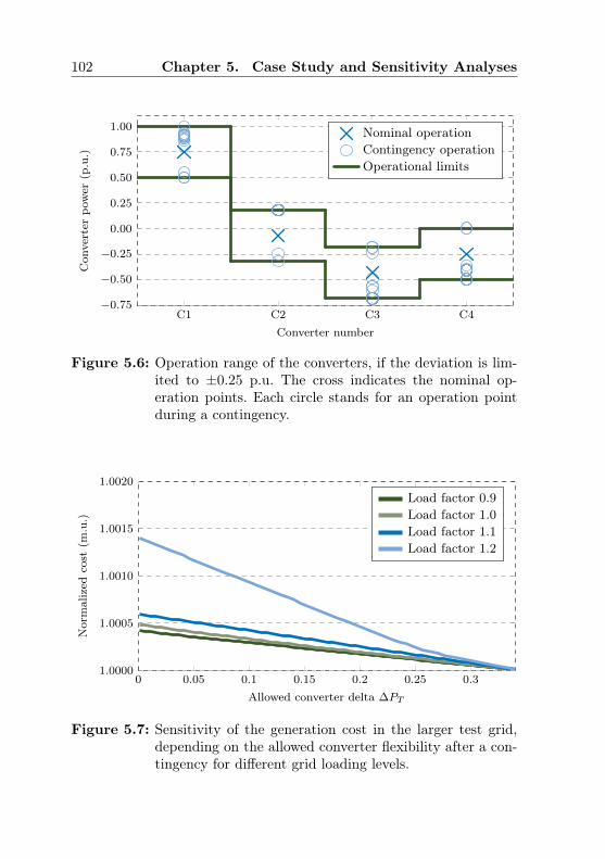
102 Chapter 5. Case Study and Sensitivity Analyses
C1 C2 C3 C4−0.75
−0.50
−0.25
0.00
0.25
0.50
0.75
1.00
Converter number
Con
vert
erpo
wer
(p.u
.)
Nominal operationContingency operationOperational limits
Figure 5.6: Operation range of the converters, if the deviation is lim-ited to ±0.25 p.u. The cross indicates the nominal op-eration points. Each circle stands for an operation pointduring a contingency.
0 0.05 0.1 0.15 0.2 0.25 0.31.0000
1.0005
1.0010
1.0015
1.0020
Allowed converter delta ∆PT
Nor
mal
ized
cost
(m.u
.)
Load factor 0.9Load factor 1.0Load factor 1.1Load factor 1.2
Figure 5.7: Sensitivity of the generation cost in the larger test grid,depending on the allowed converter flexibility after a con-tingency for different grid loading levels.

5.2. Results 103
5.2.3 Converter and DC Line Capacity
The next topic which was investigated is the required capacity of theconverters and DC lines. First an individual approach is chosen. TheDC line capacities are scaled linearly with a certain factor, while theconverter capacities are fixed, to see the influence to the operating costof the system. Second, the converter capacities are varied, while the DCline capacities stayed unchanged. Finally, the DC line and converter ca-pacities are simultaneously scaled with a linear factor and the influenceon the operating cost are investigated.
Smaller Grid
Figure 5.8 shows the change in operating cost, if the capacity of theconverters is reduced. All converter capacities are changed linearly withthe same factor. This means the cost progression from a corrective con-trolled approach to the case with security and no HVDC grid is shown.
0 0.1 0.2 0.3 0.4 0.5 0.6 0.71.00
1.10
1.20
1.30
Converter capacity factor
Nor
mal
ized
cost
(m.u
.)
Load factor 0.9Load factor 1.0Load factor 1.1Load factor 1.2
Figure 5.8: Sensitivity of the generation cost in the smaller test grid,depending on the converter capacity for different grid load-ing levels.
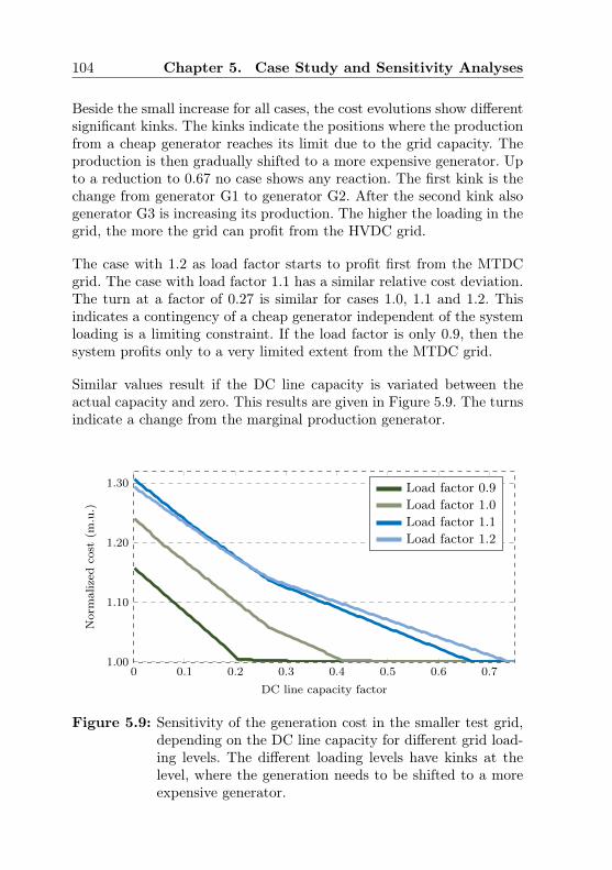
104 Chapter 5. Case Study and Sensitivity Analyses
Beside the small increase for all cases, the cost evolutions show differentsignificant kinks. The kinks indicate the positions where the productionfrom a cheap generator reaches its limit due to the grid capacity. Theproduction is then gradually shifted to a more expensive generator. Upto a reduction to 0.67 no case shows any reaction. The first kink is thechange from generator G1 to generator G2. After the second kink alsogenerator G3 is increasing its production. The higher the loading in thegrid, the more the grid can profit from the HVDC grid.
The case with 1.2 as load factor starts to profit first from the MTDCgrid. The case with load factor 1.1 has a similar relative cost deviation.The turn at a factor of 0.27 is similar for cases 1.0, 1.1 and 1.2. Thisindicates a contingency of a cheap generator independent of the systemloading is a limiting constraint. If the load factor is only 0.9, then thesystem profits only to a very limited extent from the MTDC grid.
Similar values result if the DC line capacity is variated between theactual capacity and zero. This results are given in Figure 5.9. The turnsindicate a change from the marginal production generator.
0 0.1 0.2 0.3 0.4 0.5 0.6 0.71.00
1.10
1.20
1.30
DC line capacity factor
Nor
mal
ized
cost
(m.u
.)
Load factor 0.9Load factor 1.0Load factor 1.1Load factor 1.2
Figure 5.9: Sensitivity of the generation cost in the smaller test grid,depending on the DC line capacity for different grid load-ing levels. The different loading levels have kinks at thelevel, where the generation needs to be shifted to a moreexpensive generator.

5.2. Results 105
0.250.5
0.751
0.25
0.5
0.751
1
1.05
1.1
1.15
Converter capacity factor
DC line capacity factor
Nor
mal
ized
cost
(m.u
.)
Figure 5.10: Sensitivity of the generation costs in the smaller test grid,depending on the converter capacity and DC line capac-ity for loading level of 0.9.
If the converter capacities and the DC line capacities are varied simul-taneously the interdependency can be evaluated. Figure 5.10 gives thenormalized operating cost for the case with a load factor of 0.9. As thegrid does only profit marginally from the MTDC grid, the shape in-creases towards the sides. A low level of the converter and line capacityis represented, whereas the relative increase in cost is low.
A different behavior is seen for the case with a load factor of 1.2, asshown in Figure 5.11. The cost increases significantly towards the bor-ders.
Larger Grid
The same values as for the smaller grid are given for the larger grid inFigures 5.12 and 5.13 for the converter and DC line capacities, respec-tively. The cases with load factor 1.1 and 1.2 profit most from highercapacity in the MTDC grid. At this loading the AC grid comes closerto its capacity limits.

106 Chapter 5. Case Study and Sensitivity Analyses
0.250.5
0.751
0.25
0.5
0.751
1
1.05
1.1
1.15
1.2
1.25
1.3
Converter capacity factor
DC line capacity factor
Nor
mal
ized
cost
(m.u
.)
Figure 5.11: Sensitivity of the generation costs in the smaller test grid,depending on the converter capacity and DC line capac-ity for loading level of 1.2.
The bulk transmission from the northern to the southern parts of thegrid would even profit from converters larger than the given ones forall cases. A kink in the curves is again the change from a marginalgenerator to the next, which is a function of the converter sizes.
For the DC lines a slightly different picture is visible. The capacity canbe reduced by almost 50 % before a major change is visible. The ratioof the converter to line capacity is the same as in the smaller grid. Thereason for this behavior is that the MTDC grid is more meshed in thiscase.
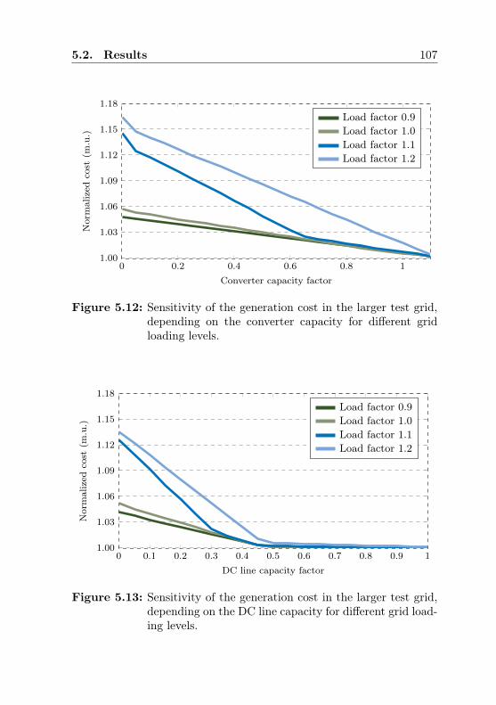
5.2. Results 107
0 0.2 0.4 0.6 0.8 11.00
1.03
1.06
1.09
1.12
1.15
1.18
Converter capacity factor
Nor
mal
ized
cost
(m.u
.)
Load factor 0.9Load factor 1.0Load factor 1.1Load factor 1.2
Figure 5.12: Sensitivity of the generation cost in the larger test grid,depending on the converter capacity for different gridloading levels.
0 0.1 0.2 0.3 0.4 0.5 0.6 0.7 0.8 0.9 11.00
1.03
1.06
1.09
1.12
1.15
1.18
DC line capacity factor
Nor
mal
ized
cost
(m.u
.)
Load factor 0.9Load factor 1.0Load factor 1.1Load factor 1.2
Figure 5.13: Sensitivity of the generation cost in the larger test grid,depending on the DC line capacity for different grid load-ing levels.

108 Chapter 5. Case Study and Sensitivity Analyses
5.3 Conclusion
This chapter provides some simulation cases and sensitivity analyses.The beforehand proposed OPF and SCOPF are applied. The two gridsshow different behaviors. The smaller grid prints out the large advantageof an added MTDC grid. The cost with and without security consider-ations can be reduced significantly. It shows that flexibility introducedby a correctively controlled MTDC grid can reduce the cost comparedto preventive control.
For the larger grid the cost for preventive and corrective control aresignificantly below the cost without the HVDC grid, but the difference isnot as large as for the small grid. Therefore, the added value of flexibilityis lower. This depends on the grid congestions, which are only a specifictransmission corridor in the latter case. This can be overcome only withbulk transmission.
Another investigation of these simulations is the ratio between the con-verters and the DC line capacities. This ratio is also case dependent,but in general the more meshed the DC grid is, the higher the ratiobetween the converters capacity and DC line capacity can be.

Chapter 6
Dynamic Control ofMulti-Terminal HVDCGrids
Besides the steady state operation of an MTDC grid, the dynamic con-trol is also of interest. This chapter presents a controller to locally con-trol the power flows in the VSC. The control objective is to share thefrequency containment reserves between asynchronous areas. First anapproach based on local measurements is given. It is expanded in twosteps by incorporating generator control and a limited communicationnetwork to achieve better performance. The chapter is based on [40],[89], [90], and [91]. The work in this chapter results from a collaborationwith Martin Andreasson [92] from KTH, Stockholm. The author’s con-tributions are the power system background and the simulations, whileMartin contributed to the controller design and mathematical stabilityproofs.
109
110 Chapter 6. Dynamic Control of MTDC Grids
6.1 Introduction to Dynamics in Multi-Terminal HVDC Grids
Existing HVDC links between AC grids are primarily used for bulkpower transfer between the AC areas. No dynamic power flow controlis applied. A possible application of the fast operation would enableservices as exchanging frequency regulation reserves between the con-nected grids. By connecting several AC grids by an MTDC system, fre-quency containment regulation reserves can be shared, which reducesthe need for frequency regulation reserves in the individual AC sys-tems [93]. Wind farms connected through HVDC links have also beenproposed to provide frequency control on connected areas [94].
One practical example of this possibility is the island of Gotland inSweden, where the first HVDC link was installed. The island is onlyconnected to the main Nordic grid through an HVDC cable [24,95].However, since the main Nordic AC grid has inertia orders of magni-tudes higher than the AC grid of Gotland, the influence of frequencyregulations on the main grid will be negligible. When connecting twoor more AC grids of similar size or different order of magnitude, theinfluence on the other AC grids must be taken into account when usingHVDC links to share frequency containment reserves.
Maintaining an adequate DC voltage is the most important practicalcontrol problem in HVDC transmission systems. If the DC voltage de-viates too far from the nominal operational voltage, equipment could bedamaged, resulting in loss of power transmission capability and highercost.
In [96] distributed control algorithms have been applied to share fre-quency containment control reserves of asynchronous AC systems con-nected through an MTDC system. However, the proposed controllerrequires a slack bus to control the DC voltage which is a drawback,especially for large grids. In [97,98] distributed controllers for frequencycontainment control of MTDC systems are proposed. They have the ad-vantage that they do not rely on a slack bus. Both of the aforementionedcontrollers however rely on the presence of a communication network.
While a communication network might already be present, it introducesthe issue of time delays due to large geographical distances in MTDCsystems. It also has an outage risk, especially in case of a contingency.

6.1. Introduction to Dynamics in MTDC Grids 111
If it is an external cause, e.g. weather, earthquake or construction ma-chines, it could influence the communications system too, either inter-rupt or at least disturb it. The impacts of delays have been analyzedin [99]. They have been found to seriously degrade performance anddestabilize the power system.
A distributed controller without the need of a slack bus is proposed in[96]. Stability of the equilibrium is guaranteed in the absence of commu-nication delays. However, the voltage dynamics of the HVDC system areneglected. Moreover, the implementation of the controller is not realis-tic as every controller needs to access the DC voltages of all convertersinstantaneously.
Two other cases with decentralized controllers sharing frequency con-tainment reserves are [100] and [101]. In [100] no stability analysis ofthe closed-loop system is performed, whereas [101] guarantees stabilityof the equilibrium provided that the connected AC areas have identicalparameters. In [102] optimal decentralized controllers for AC systemsconnected by HVDC systems are derived. In all aforementioned refer-ences the voltage dynamics of the HVDC system are neglected.
To avoid the inherent difficulties of time delays a decentralized propor-tional controller for sharing frequency containment reserves is proposed.It relies only on local measurements in the basic version. The controllergoal is to distribute the frequency control reserves between the con-nected AC systems while maintaining an adequate DC voltage.
The basic controller version without communication works for a firstapproach, but has some disadvantages concerning the long term per-formance. These can be overcome by using a communication systemto exchange data on a slower time scale. A better performance can beachieved if the generators of an area are informed by the controller assoon as it changes the power setpoint of the converter. The generatorscan react already before the grid frequency deviation shows the full ex-tent of the imbalance. To bring back the frequency to the nominal value,an extended version of the controller is required. This controller is basedon a reduced communication grid.

112 Chapter 6. Dynamic Control of MTDC Grids
6.2 Distributed Controller for Multi-Termi-nal HVDC Grids
First the three controllers are explained and later a simulation study forall controllers is given. There exist mathematical stability proofs for allthree controllers described here. A simplified system is used to show thestability of the combined AC and DC systems including the proposedcontrollers. The details of the proofs can be found in [103].
6.2.1 Controller 1 – Local Converter Controller
The proposed basic controller in [40] uses the deviation from the definedfrequency ωref,c in the AC grid and the deviation of the voltage setpointuDC
ref,i. Both deviations can be scaled to achieve different controller out-puts. The controller can then be formulated as follows:
pvsc,c = pvsc,set,c +Kωc
(ωc − ωref,c
)+Ku
c
(uDC
ref,c − uDCc
)(6.1)
The given power setpoint from the grid controller Pvsc,set,c, for examplefrom a SCOPF calculation, is the first term of the controller. The scaleddeviation from the frequency is the second term and the scaled deviationfrom the DC voltage the third one. Kω
c ≥ 0 and Kuc ≥ 0 are positive
controller gains for all c = 1, . . . , nvsc. This gives the new setpoint forthe power injections at this converter, pvsc,c. The physical limits of theconverter have to be incorporated as well. The output of (6.1) has to belimited to the converter minimum and maximum capacities. This willnullify the stability proofs.
This method works as a double droop controller. This means also adisturbance in the DC grid will influence the connected AC grids. Asimplified explanation how the Controller 1 (6.1) reacts, is describedbelow. Only two converters from different asynchronous AC areas areconsidered for this example.
• Area 1 has a frequency drop due to a disturbance.
• the second term in (6.1) becomes negative and the converter re-duces the amount of exported power from the AC grid to the DCgrid.

6.2. Distributed Controller for MTDC Grids 113
• this helps Area 1 to stabilize its frequency.
• the DC voltage at converter 1 starts to reduce due to the reducedinfeed.
• the DC voltage is spread over the grid and the third term in (6.1)of the second converter becomes positive. The second converterdetects the reduced voltage also at its side and increases the infeedto the DC grid.
• the higher consumption in Area 2 will lead to a reduction of thefrequency.
• this will in principle continue until a new equilibrium is found.
This controller works fine as a first reaction in case something happensin the combined grid. Since the converters react much faster than thegenerators, the consequences for the area suffering a contingency canthus be limited. The generators react only on the new frequency andnot on the changes in the converter, which takes some time. To compen-sate this effect a signal has to be generated as an additional input forthe generator setpoints to balance the areas after a contingency. Thisprinciple is considered in the next controller.
6.2.2 Controller 2 – Combined Converter and Gen-erator Controller
The idea of the second controller explained in [90] is to ensure a reactionalso from the generators in all connected areas and therefore tightenthe stationary error bounds of the system after a contingency. This canonly be achieved if the different AC areas coordinate their reaction. Thecoordinated reaction between different areas requires a communicationgrid, whose dynamics can be quite slow. Two general communicationconcepts are possible and shown in Figure 6.1.
There are different possibilities to construct the communication grid(dashed blue lines) for the controller. Figure 6.1a (a) shows a completegraph, which is in general denser than the MTDC grid (solid greenlines). This grid allows a centralized controller, since all connections areavailable. Figure 6.1a (b) shows the reduced communication system,

114 Chapter 6. Dynamic Control of MTDC Grids
AC 1
AC 2
AC 3
AC 6 AC 4
AC 5
(a)
AC 1
AC 2
AC 3
AC 6 AC 4
AC 5
(b)
Figure 6.1: Illustration of six AC grids connected with an HVDC gridand a communication network with different topologies.The HVDC lines are illustrated with green solid lines,while communication lines are illustrated with blue dashedlines. (a) Shows the structure of the complete communi-cation structure of controller (6.2), while (b) shows an ex-ample for the structure of the distributed communicationstructure of controller (6.4).
which has to be at least a connected graph, connection all nodes. Allintermittent solutions are also possible.
A contingency or the large distances in the HVDC grid could also lead toa reduced communication system, an example is shown in Figure 6.1b. Insuch a system each converter has active communication with at least oneof its neighbors. With this setup a distributed controller scheme has tobe used. Any possible transition between these two systems is possible.These two communication systems between the areas are the basis forthe controller laws. Inside the areas all generators can communicatewith the converter of the same area.
The converter controller (6.1) still gives the power setpoints for theconverters. Additionally, the AC generators are controlled with the fol-lowing controllers.
The centralized generation controller of the AC systems is given by:

6.2. Distributed Controller for MTDC Grids 115
pgenp = pgen
set,p −Kdroopp
(ωp − ωref,c
)− Ku
c
Kωc
K ic
1
nvsc
nvsc∑i=c
ηc (6.2)
ηc = K ic
(ωc − ωref,c
)− κηc (6.3)
where κ, K ic, ∀ c = 1, . . . , nvsc are positive constants. If κ = 0, then
ηc becomes a scaled integral state of the local frequency deviation(ωc − ωref,c). The controller (6.2) can be interpreted as a combinedfrequency droop controller and second layer frequency control whichalso incorporates the states from remote areas. Depending on the exist-ing droop controller of the generator, the second term of (6.2) can beneglected.
The distributed generation controller of the AC systems is given by:
pgenp = pgen
set,p −Kdroopp
(ωp − ωref,c
)− Ku
c
Kωc
K icηc (6.4)
ηc = K ic
(ωp − ωref,c
)−∑j∈Nc
ccj
(ηc − ηj
)(6.5)
We assume ccj = cjc, i.e. the communication graph is undirected. Ncis the set of all neighboring converters, which are connected with acommunication line. The above controller can be interpreted as a dis-tributed PI-controller, with a distributed consensus filter acting on theintegral states ηc. In contrast to the controller (6.2)-(6.3), (6.4)-(6.5) isdistributed. Note, that there is no assumption that the communicationtopology resembles the physical topology of the MTDC system.
Both controllers lead to a fast reaction from the converters according to(6.1), which is then supported by the generators in the correspondingarea. The controllers have comparable performance as later shown inthis chapter by simulations.
These two controllers reduce the frequency deviations in the grids, butthere is still a steady state error remaining due to the double droopdesign and the lack of coordination of the converter controller. To drivethe frequencies back to the nominal values an additional modificationhas to be made. This is considered in the next controller.

116 Chapter 6. Dynamic Control of MTDC Grids
6.2.3 Controller 3 – Extended Controller for Con-verter and Generator
To bring back the frequency to its nominal value, adjustments in theconverter controller are needed. The controller (6.1) is expanded by anauxiliary controller term. The new converter controller governing thepower injections from the AC systems into the HVDC grid is then givenby:
pvsc,c = pvsc,set,c +Kωc
(ωc − ωref,c
)+Ku
c
(uDC
ref,c − uDCc
)+∑j∈Nc
cφcj
(φc − φj
)(6.6)
φc =Kωc
Kuc
ωc − γφc (6.7)
where γ > 0 and cφcj = cφjc > 0. The converter controller (6.6)-(6.7) canbe interpreted as an emulation of an AC network between the isolatedAC areas. The auxiliary controller variables φc can be thought of asthe phase angles of AC area c, governing the power transfer betweenthe areas. The control system works similar to an automatic generationcontrol (AGC) system in the AC grid [104]. In contrast to an AC system,the power is fed into the HVDC grid instead of being directly transferredto the neighboring AC areas. Note that also the reference voltages uDC
ref,care not necessarily uniform, as with the reference frequency ωref,c. Thegenerators are still controlled with the controller (6.4).
This leads to a system without any steady state errors in the frequenciesafter a contingency. The performance of all controllers is shown in thenext section by simulations.
6.3 Simulation
All three above explained control systems are tested in a simulationstudy described in this section.
6.3.1 Simulation Framework
The used framework for the simulations is a phasor model taken from[105], which was also used in [106]. The power system is represented by

6.3. Simulation 117
a hybrid system capturing nonlinear continuous and discrete dynamics.In such hybrid systems “there is such a strong coupling between thesediscrete and continuous behavior of the system, so that they must beanalyzed simultaneously” [105].
The system is solved by using differential switched algebraic and statereset equations (DSAR) formulation.
sx = f(sx, sy, sz,λ) (6.8)
sz = 0 (6.9)
0 = g(0)(sx, sy, sz) (6.10)
0 =
g(i−)(sx, sy, sz,λ) ys,i ≤ 0
g(i+)(sx, sy, sz,λ) ys,i ≥ 0i = 1, . . . , ss (6.11)
sz+ = hj(sx
−, sy−, sz
−,λ) yr,j = 0 j = 1, . . . , sr (6.12)
where sx are continuous dynamic states, sz are discrete states, sy arealgebraic states and λ are parameters. The values for pre-event valuesare marked with the superscript −, the one for post-event values aremarked with +. More details about the framework are given in [105].
6.3.2 Study Grid Topology
The used grid in this simulation is shown in Figure 6.2. It is based on sixtimes the IEEE14 bus test system [71], where each of this asynchronousareas have one VSC station. Each of the octagon stands for a complete14 bus AC grid. They are connected to different AC buses as stated inFigure 6.2. The HVDC grid consists out of nine transmission lines withdifferent lengths. The grid parameters are given in the Appendix C.3.
The simulated case is a generator outage at bus 2 in Area 1 of 0.2 p.u.The remaining generation capacity at this bus is still available. Theoutage is about 6 % of the total load of one area. Therefore the impacton the system is quite significant. Higher disturbances would increasethe effect even more until the system would collapse. This effect was notinvestigated in this simulations, but it is assumed that the system canwithstand larger outages with the HVDC grid controller than without.

118 Chapter 6. Dynamic Control of MTDC Grids
1
2 3
4
5
6
7
8
9
1011
12 13 14
AC Area 4
AC Area 1
bus 1C1
AC Area 2
bus 2C2
AC Area 3
bus 4
C3
AC Area 4
bus 1C4
AC Area 5
bus 5C5
AC Area 6
bus 3C6
MTDC Grid
Figure 6.2: Test grid for dynamic simulations. Six asynchronousIEEE14 bus test cases connected with an MTDC grid.Each octagon represents a full 14 bus AC grid, as shown inthe lower part of the figure. The connection bus of the VSCstation is individual and given in the figure. The MTDCgrid is represented by the green lines. The dashed bluelines indicate the used reduced communication grid.

6.3. Simulation 119
ci
rijiij
lij
cj
ui uj
iinji
iinjj
Figure 6.3: RL-line model of a DC transmission line. Each converterhas a capacity ci to stabilize the voltage. The line itself ismodeled as a resistor rij and an inductor lij .
6.3.3 Simulation Models
All generators are modeled as standard 6th-order synchronous machinemodel [58], with the parameters given in Tables C.13 and C.14. Agovernor (GOV) and an automatic voltage regulator (AVR) is attachedto the generator to control the power and voltage output. The modelsused are described in [107].
The AC lines are modeled by a series of RL branches with different RLvalues [105]. The DC lines are modeled as single RL connections, asshown in Figure 6.3. This figure also shows that each VSC converterhas a capacitance on the DC side.
The converters themselves are not modeled dynamically, since the timeconstant is orders of magnitudes faster than the rest of the system dy-namics. They are only a power balance connection between the AC andDC side. On the DC side a capacitance limits the changes in voltagesand adds therefore some dynamic responds. On the AC side, the con-verter is connected with a reactance to the next AC bus. The loads aremodeled as constant power loads.
6.3.4 Controller Parameters
The used controller parameters are given in Table 6.1. They were definedmanually by the evaluation of several different simulation studies. For

120 Chapter 6. Dynamic Control of MTDC Grids
all controllers the same values are chosen, which seems reasonable sinceall the grids have the same size and similar structure.
The controllers work as a controllable firewall and the parameter can bechosen depending on the size and behavior of the connected AC grids.If one area has more fast controllable power plants, it is plausible tohave a lower sensitivity to spread faults to the MTDC grid than an areawith only slow controllable power plants.
6.3.5 Results Controller 1 – Local Converter Con-trol
Frequency
The first simulation was done with controller (6.1). The frequencies ofall 30 generators in the six areas are shown in Figure 6.4, where eacharea has its own color. Inside each area the individual frequencies areclose together. Therefore, the single generators are hard to detect. Themagnification shows that in Area 1 some oscillations are present, butthey are small compared to the overall area oscillations. The reasoningfor the absence of oscillations within each area is the small electricaldistance between the generators, since the used grid has not a largeextension and all generators are in the southern half of the grid.
The case without HVDC controller has the largest overall deviationby far. This was expected, since only the generators in Area 1 cancounteract the disturbance. In the case with the HVDC controller, thepeak deviation is significantly smaller. Area 1, where the outage occurs,shows the highest deviation. The reaction of the others depends on theirMTDC grid distance to Area 1. Area 2 and 3 are direct neighbors andshow the largest deviation, followed by Area 4 and 5. The smallest devi-ation occurs in Area 6. This is explained by the long transmission lines
Table 6.1: Controller parameters for all three proposed controllers.
Kωc Ku
c Kdroopp K i
c cηcj cφcj κ γ
1501 80 9 4.5 5/rij 15/rij 0 0
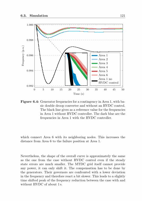
6.3. Simulation 121
0 5 10 15 20 25 30 35 40 45 50
0.992
0.994
0.996
0.998
1.000
Time (s)
Freq
uenc
y(p
.u.)
Area 1Area 2Area 3Area 4Area 5Area 6Area 1 noHVDC control
0 5 10 15 20 25 30 35 40 45 50
0.992
0.994
0.996
0.998
1.000
Time (s)
Freq
uenc
y(p
.u.)
Area 1Area 2Area 3Area 4Area 5Area 6Area 1 noHVDC control
Figure 6.4: Generator frequencies for a contingency in Area 1, with ba-sic double droop converter and without an HVDC control.The black line gives as a reference value for the frequenciesin Area 1 without HVDC controller. The dark blue are thefrequencies in Area 1 with the HVDC controller.
which connect Area 6 with its neighboring nodes. This increases thedistance from Area 6 to the failure position at Area 1.
Nevertheless, the shape of the overall curve is approximately the sameas the one from the case without HVDC control even if the steadystate errors are much smaller. The MTDC grid itself cannot provideany power, it can only shift it. The compensation has to be done bythe generators. Their governors are confronted with a lower deviationin the frequency and therefore react a bit slower. This leads to a slightlytime shifted peak of the frequency reduction between the case with andwithout HVDC of about 1 s.

122 Chapter 6. Dynamic Control of MTDC Grids
DC Voltage
The other local measurement values are the voltages in the DC grid.The voltage behavior of all converters is shown in Figure 6.5.
Area 1, reacts first with importing power from the DC grid. As a result,the voltage starts to drop. Shortly afterwards the voltage drop arrivesto the other areas consecutively and they start to feed in more powerto the MTDC grid. The voltage oscillation is stabilized, and the newequilibrium is at a lower voltage magnitude between 0.985 and 0.992 p.u.
The voltage curves show the same behavior as the frequency. The highestdeviation is in Area 1, followed by the others up to Area 6 which isfurthest away.
0 5 10 15 20 25 30 35 40 45 500.970
0.975
0.980
0.985
0.990
0.995
1.000
Time (s)
DC
volt
age
(p.u
.)
Area 1 Area 2 Area 3Area 4 Area 5 Area 6
Figure 6.5: DC voltages for a loss of 0.2 p.u. generation in Area 1with double droop converter control. The most significantreaction occurs in Area 1 (dark blue), where the contin-gency happens. The other areas react according to theirelectrical distance to the failure.

6.3. Simulation 123
Converter Flows
The deviations in frequency and DC voltage as input for the local VSCcontroller (6.1) lead to the converter flows shown in Figure 6.6.
The results in the figure clearly show the flexibility and fast reactiontime of the HVDC grid. Within 2 s all converters have reached their newpower flows, with only some small oscillations. Then a slow adoptionprocess begins which results in a new equilibrium of the power flows. Theduration of this process is related to the ramping time of the generators.Finally, converter C1 imports 0.15 p.u. and all the others export roughly0.03 p.u. each. This means about 75 % of the failing generation capacityis compensated outside of Area 1.
0 5 10 15 20 25 30 35 40 45 50
−0.15
−0.12
−0.09
−0.06
−0.03
0.00
0.03
Time (s)
Con
verter
flow
(p.u.)
Area 1 Area 2 Area 3Area 4 Area 5 Area 6
Figure 6.6: Converter flows for a loss of 0.2 p.u. generation in Area 1with double droop converter control. Area 1 (dark blue)react in decreasing its power flow from the HVDC grid,to about -0.15 p.u.. This is compensated by all the otherconverters, which contribute on average 0.03 p.u. more tothe HVDC grid.

124 Chapter 6. Dynamic Control of MTDC Grids
Generator Outputs
The behavior of the generators is shown in Figure 6.7. It shows the sumof all generators of each area. The solid lines show the electrical outputof the generators. There is a spike at the beginning, due to the voltagedrop of the disturbance. The effect of the fast changing power flows inthe converters give a similar effect to all the other generators.
The dashed lines correspond to the mechanical power of the generators.They are obviously much slower and smoother than the electrical ones,but have the same steady state values.
0 5 10 15 20 25 30 35 40 45 500.00
0.02
0.04
0.06
0.08
0.10
Time (s)
Sum
ofge
nera
tor
outp
utde
viat
ions
(p.u
.)
Area 1 Area 2 Area 3Area 4 Area 5 Area 6
Figure 6.7: Electrical (solid lines) and mechanical (dashed lines) powerdeviations per area for a loss of 0.2 p.u. generation inArea 1 with only basic double droop converter control.Area 1 (dark blue) reacts first, followed by all other areas.All areas show the same behavior for electrical and me-chanical power and diverge only in the magnitude of thereaction.

6.3. Simulation 125
6.3.6 Results Controller 2 – Combined Converterand Generator Controller
The second simulation study was done with controller (6.1) applied forthe converters, (6.2)-(6.3) for the centralized control and (6.4)-(6.5) forthe distributed control. The control goal is to get the average frequenciesand DC voltages closer to their nominal values. This section presents acomparison between Controller 1 and Controller 2.
Frequency
The reaction of the frequencies is shown in Figure 6.8. The solid lines arethe frequencies in the centralized version and the dashed lines representthe values for the distributed control. For comparison the dotted linegives the frequencies for generators in Area 1, if only the convertercontroller is active.
It is noted that the results of the centralized and distributed controllerare very close together with only some small deviations. The central-ized controller has higher frequency deviations in Area 1, due to theterm η in (6.2), which has an equalizing effect over all areas. Therefore,the reaction of the generator is damped, compared with the distributedcontroller, where only Area 2 is considered. The transfer of the voltagedeviation through the DC grid is fast and therefore almost similar tothe communication grid. The generators in the other areas start pro-ducing more, since the overall system is short in power. Therefore, localfrequencies settle the values slightly above 1 p.u. This gives an averagefrequency of exactly 1 p.u.
Compared to the converter only controller, the deviation to the nominalfrequency for Area 1 is only a third. This is a significant improvementand shows the advantage of this controller.

126 Chapter 6. Dynamic Control of MTDC Grids
0 5 10 15 20 25 30 35 40 45 500.9979
0.9982
0.9985
0.9988
0.9991
0.9994
0.9997
1.0000
1.0003
Time (s)
Freq
uenc
y(p
.u.)
Area 1Area 2Area 3Area 4Area 5Area 6
0 5 10 15 20 25 30 35 40 45 500.9979
0.9982
0.9985
0.9988
0.9991
0.9994
0.9997
1.0000
1.0003
Time (s)
Freq
uenc
y(p
.u.)
Area 1Area 2Area 3Area 4Area 5Area 6
Figure 6.8: Generator frequencies for a loss of 0.2 p.u. generation inArea 1, with coordinated converter and generator control(Controller 2). The dotted dark blue line gives the frequen-cies for Area 1 with Controller 1 as a reference value. Thesolid lines are the frequency with the centralized controllerand the dashed lines are the frequency with the distributedcontroller.

6.3. Simulation 127
DC Voltage
The actual goal of this controller is to bring the DC voltages back to anaverage value of 1 p.u. The DC voltages from the converters are shownin Figure 6.9, again solid for distributed and dashed for central control.
In this case the same picture as with the frequencies can be seen. Thedifferences in DC voltages between the central and distributed controllerare marginal. The voltage at converter C2 to C6 are above the nomi-nal voltage, but the system average voltage is 1 p.u. The deviation atconverter C1 is again only about a third of the deviation which occurswith the Controller 1.
0 5 10 15 20 25 30 35 40 45 500.970
0.975
0.980
0.985
0.990
0.995
1.000
1.005
Time (s)
DC
volt
age
(p.u
.)
Area 1 Area 2 Area 3Area 4 Area 5 Area 6
Figure 6.9: DC voltages for a loss of 0.2 p.u. generation in Area 1with coordinated converter and generator control (Con-troller 2). The dotted dark blue line gives the frequenciesfor Area 1 with Controller 1 as a reference value. The solidlines are the frequency with the centralized controller andthe dashed lines are the frequency with the distributedcontroller.

128 Chapter 6. Dynamic Control of MTDC Grids
Converter Flows
Figure 6.10 shows the converter flows. Again the same display style isused. It is seen that the flows in the converters are slightly lower forthe second controller structure, for both the central and the distributedapproach. Also a stable operation point is achieved earlier. This can bereached due to the coordinate control resulting in a faster reaction ofthe generators.
0 5 10 15 20 25 30 35 40 45 50
−0.15
−0.12
−0.09
−0.06
−0.03
0.00
0.03
Time (s)
Con
verter
flow
(p.u.)
Area 1 Area 2 Area 3Area 4 Area 5 Area 6
Figure 6.10: Converter power for a contingency in Area 1 with coordi-nated converter and generator control (Controller 2). Thedotted dark blue line gives the converter flow for Area 1with Controller 1 as a reference value. The solid lines arethe converter power with the centralized controller andthe dashed lines are the frequency with the distributedcontroller.
Generator Outputs
The generator outputs are shown in Figure 6.11. Again the electricaloutputs are solid lines for central controller and dashed lines for dis-tributed one. All mechanical outputs are marked as dash-dotted lineswith the same color. The dotted line is the electrical output from Area 1

6.3. Simulation 129
for the basic converter control, Controller 1. All outputs look quite simi-lar, but small differences occur. The major change between the convertercontrol (Controller 1) to the two others is marked with the magnifier.The dotted line leaves the rectangular to the right and slowly increasesafterward, whereby the solid and dashed line goes directly up, which re-flects a higher generation at this time. Therefore, the second controllerhas less frequency deviations although the converter flows are lower.The generators are informed about the deviations and can react beforethey see the full extent of the frequency deviation.
0 5 10 15 20 25 30 35 40 45 500.00
0.02
0.04
0.06
0.08
0.10
Time (s)
Sum
ofge
nera
tor
outp
utde
viat
ion
(p.u
.)
Area 1 Area 2Area 3 Area 4Area 5 Area 6
0 5 10 15 20 25 30 35 40 45 500.00
0.02
0.04
0.06
0.08
0.10
Time (s)
Sum
ofge
nera
tor
outp
utde
viat
ion
(p.u
.)
Area 1 Area 2Area 3 Area 4Area 5 Area 6
Figure 6.11: Electrical and mechanical power output deviation for aloss of 0.2 p.u. in area 1 with coordinated converter andgenerator control. The electrical (dotted) and mechanical(dashed) power for Area 1 (dark blue) with Controller 1 isgiven as a reference value. The solid lines are the electricalpower output with the Controller 2 and dashed-dottedlines are the mechanical power. The magnifier shows thedifferent reaction shortly after the contingency.

130 Chapter 6. Dynamic Control of MTDC Grids
6.3.7 Results Controller 3 – Extended Controller forConverter and Generator
The last controller is the extended version of the combined generator andconverter controller (6.6)-(6.7). The drawback of the second controllerwas the steady state error in the frequencies. This is now avoided asshown in the results.
Frequency
The frequency behavior of the areas is now different as shown in Fig-ure 6.12. All generator frequencies of each area are plotted as solid lines.In addition, the dashed line shows the frequency of Area 1 for the Con-troller 2 in the distributed version. The dotted line is the frequency inArea 1 for the Controller 1.
The control goal of the converter is reached, as all frequencies are goingback to 1 p.u., after about 30 s a stable operation point is reached.The frequencies of the individual areas are already synchronized before.This is followed by some oscillations at the beginning, as shown in themagnification, but after 5 s all frequencies are equivalent.

6.3. Simulation 131
0 5 10 15 20 25 30 35 40 45 500.9982
0.9985
0.9988
0.9991
0.9994
0.9997
1.0000
Time (s)
Freq
uenc
y(p
.u.)
Area 1Area 2Area 3Area 4Area 5Area 6
0 5 10 15 20 25 30 35 40 45 500.9982
0.9985
0.9988
0.9991
0.9994
0.9997
1.0000
Time (s)
Freq
uenc
y(p
.u.)
Area 1Area 2Area 3Area 4Area 5Area 6
Figure 6.12: Generator frequencies for a loss of 0.2 p.u. generation inArea 1 with the extended converter and generator con-trol (Controller 3). The dotted line is the reaction of thefrequencies in Area 1 (dark blue) for Controller 1, thedashed line is for Controller 2. The solid lines show thevalues for all areas with Controller 3. The magnifier showsthe small oscillations shortly after the contingency hashappened.

132 Chapter 6. Dynamic Control of MTDC Grids
DC Voltage
The six DC voltages are shown in Figure 6.13. The average voltage inthe grid is controlled to 1 p.u. and the deviation for the Area 1 is higherthan in the case for the second controller. This is required to ensure thehigher flows as shown in the next paragraph.
0 5 10 15 20 25 30 35 40 45 500.970
0.975
0.980
0.985
0.990
0.995
1.000
1.005
Time (s)
DC
volt
ages
(p.u
.)
Area 1 Area 2 Area 3Area 4 Area 5 Area 6
Figure 6.13: DC voltages for a loss of 0.2 p.u. generation in area 1with the extended converter and generator control (Con-troller 3). The dotted line is the reaction of the DC volt-age in Area 1 (dark blue) for Controller 1, the dashedline is for Controller 2. The solid lines show the valuesfor all areas with Controller 3.

6.3. Simulation 133
Converter Flows
The converter flows are shown in Figure 6.14. The flow at converterC1 is significantly higher, than for the other cases. All other convertershave similar power flow of 0.033 p.u., which is exactly a sixth of thedisturbance. This represents the ideal power sharing between the sixareas. This values are stable after about 7 s.
0 5 10 15 20 25 30 35 40 45 50
−0.18
−0.15
−0.12
−0.09
−0.06
−0.03
0.00
0.03
0.06
Time (s)
Con
verter
flow
(p.u.)
Area 1 Area 2 Area 3Area 4 Area 5 Area 6
Figure 6.14: Converter flows for a contingency in Area 1 with the ex-tended converter and generator control (Controller 3).The dotted line is the reaction of the converter power inArea 1 (dark blue) for Controller 1, the dashed line is forController 2. The solid lines show the values for all areaswith Controller 3.

134 Chapter 6. Dynamic Control of MTDC Grids
Generator Outputs
The same effect is also visible at the generator outputs as shown inFigure 6.15. Each area has exactly the same change of 0.033 p.u. AlsoArea 1 participates only with this factor, although it has the disturbancein its own area.
This is in line with the absence of a frequency deviation between theareas. Therefore, the change in generation has to be fully compensatedby the generators.
0 5 10 15 20 25 30 35 40 45 500.00
0.02
0.04
0.06
0.08
0.10
Time (s)
Sum
ofge
nera
tor
outp
utde
viat
ions
(p.u
.)
Area 1 Area 2Area 3 Area 4Area 5 Area 6
Figure 6.15: Electrical and mechanical power output deviation fora loss of 0.2 p.u. in area 1 with coordinated converterand generator control. The electrical power for Area 1(dark blue) with Controller 1 (dotted) and Controller 2(dashed) are given as a reference value. For Controller 3the electrical power (solid lines) and the mechanicalpower (dashed dotted) are given.
To summarize, Controller 3 fulfills its goals. All frequencies are goingback to their nominal values and the deviation is perfectly shared be-tween all connected areas.

6.4. Conclusion 135
6.4 Conclusion
Controller 1, (6.1) works well and has the advantage that no commu-nication is required. It has the largest deviations for the frequency andvoltages of all presented controllers and significant frequency steadystate errors in all areas. The second controller (6.2)- (6.3) or (6.4)-(6.5),combined with (6.1) has a much better performance. The frequencysteady state errors for Controller 2 are only a third of the Controller 1deviations and the average voltage in the DC grid is at the nominalvalue. Controller 3 consisting of (6.2)-(6.3) or (6.4)-(6.5) combined with(6.6)-(6.7) brings back the frequencies to nominal value and guaranteesa perfect sharing of the power outage. It is possible to operate the con-verters shortly after a disturbance with the Controller 1 and switch toa more advanced version, if the communication grid is available andstable.
Further research would be to add an additional control loop, such asa frequency restoration control. The task of this control loop wouldbe to bring back the generation to nominal values. After the initialstabilization, Area 1 can slowly take over the full compensation, whileall the other generators are released and the flows coming from thecontrollers in the MTDC grid are back to zero. The AGC concept hasto be expanded and not only incorporate the frequencies, but also thepower flows. Another not considered part is the reactive power controlon the AC side which could offer interesting control opportunities tostabilize the voltage in the AC grid after a contingency has happened.


Chapter 7
Conclusion and Outlook
7.1 Conclusion
The first battle in the war of currents was won by AC. Nowadays thependulum is swinging back to the other side and DC gets back the morepromising role, at least for long distance power transmission. The fu-ture power systems could contain meshed MTDC grids, since they haveimportant technological advantages compared to existing AC systems.The implementation of such new system components will increase thecontrollability of existing transmission systems. This thesis delivers thebasic tools to incorporate such MTDC grids into existing AC grids. Thepower flow for combined AC and DC grids are elaborated and two meth-ods to derive optimal power setpoints for the converters and generators,if appropriate, are shown.
A nonlinear formulation for OPF problems for combined grids is de-veloped, which is computationally expensive. Since it is a non-convexproblem there is no proof for a global minimum. Therefore, a linearizedversion of the OPF formulation is presented as well. This model neglectsthe physical losses. Therefore, it is hard to allocate the flows betweenthe AC and the DC grid. By including penalty terms for AC and DCline flows, as well as for converter flows, the physical losses can be rep-resented in the objective function and the line flows are reduced main-taining the optimal generation dispatch. If appropriate penalty terms
137

138 Chapter 7. Conclusion and Outlook
are chosen, the flows in the grid are a good approximation of the orig-inal nonlinear problem. This is verified by the case studies which showonly small deviations. The quadratic objective function with only linearconstraints can be solved much more efficiently and a global minimumcan be guaranteed.
For both OPF formulations, security aspects were considered as well.The formulation for SCOPF fulfills the N-1 criterion. The preventiveand corrective control methods for the converter setpoint are intro-duced. The preventive control builds up controllable failure barriers,between the AC and DC grid. The corrective control handles the casewere the converter setpoints are adjusted after a contingency. This ap-proach shows better performance than the preventive approach, sincethe transmission capacity reserves are significantly lower on the AC andDC lines as well as in the converters. It is shown how the operatingcost of the two test cases are influenced by the flexibility of the convert-ers. Therefore, it is proposed that the future TSO of the combined gridshould be able to utilize it with at least limited corrective control aftera contingency.
This thesis proposes also a controller to share frequency containmentreserves between different asynchronous AC areas. The basic versionrelies only on local measurements and can therefore stabilize the overallsystem without communication system. The double droop control shapeleads to a steady state control error of the frequencies. To increasethe performance, the controller was expanded to incorporate also thegenerators. Otherwise they would react only on the frequency in theirown area. A significant increase in the performance could be achieved.Finally, an expanded controller is proposed which corrects the steadystate error by using a reduced communication system.
The OPF formulations are a basic requirement to build an MTDC gridin the future. They are necessary to plan and operate combined ACand meshed MTDC grids. The proposed controller to share frequencycontainment reserves shows an example of the value-increase of the flex-ibility introduced by a meshed MTDC grid.

7.2. Further Research 139
7.2 Further Research
Since there is no meshed MTDC grid built by now, there is still sometime to investigate the planning and operational prerequisites. Someinteresting research questions, which could not be implemented in thiswork, are formulated here as inspiration for future projects.
For the OPF and SCOPF formulations:
• the loss model of the VSC converters in steady state should beinvestigated, since it is a major source of losses. There is a lot ofdevelopment going on and the structure has changed from two orthree level converters towards MMCs.
• relaxation methods could be applied to reduce the complexity tocalculate the solutions for the SCOPF. They exist already for theAC grid [108,109], but not for combined AC and DC grids. Thiscould improve the calculation speed and ensure a global minimumalso in the accurate nonlinear case.
• a side project about the preferred topology of an MTDC was donein [110]. But the research was limited to pre- and post-contingencyOPF and short circuit behavior. This model could be expandedto incorporate other parameters for example protection, flexibility,simplicity, and costs.
• the proposed formulations can be applied to find suitable algo-rithms to define the optimal location to place the VSC in an ex-isting AC grid. This could also depend on other quantities likereactive power support or the flexibility as it is proposed in [111].
For the dynamic controllers:
• the influence of time delays to the reduced communication gridshould be investigated. It would be interesting to see which timeinterval can still be handled by the controller and if there is a limitto achieve a reasonable performance.
• more studies are required to show the influence of converter orline outages to the controller performance. This could also showthe reaction of the controller if the physical limit of one converteris reached.

140 Chapter 7. Conclusion and Outlook
• the reactive power control was neglected in this thesis. Since theflexibility of the converters is not limited to the active power set-point, it would be favorable to include reactive power control aswell. This could stabilize the connected AC grid after a contin-gency.
• in general, the interaction of such a control system with the ac-tual control system installed in AC grids should be investigatedin detail, especially the interaction with the AGC controller.
• all the results are based on simulations. It would be interesting toimplement this controller in a laboratory hardware DC test gridwith a few converters and compare the measurement results withthe simulations.

Appendix A
Additional Information toOptimal Power Flow
Definitions of Parameters
ykm =1
zkm= gkm + jbkm (A.1)
where
gkm =rkm
r2km + x2
km
(A.2)
bkm = − xkmr2km + x2
km
(A.3)
141

142 Appendix A. Additional Information to OPF
Flexibility Consideration in Objective Function
Figure A.1 gives the function values for different values of Π in theobjective function given in (3.20). The parameter Π can be chosen toweight the benefit for flexibility in the objective function compared toother terms. High values of Π will provide solutions away from thelimits pAC
vsc,min,c and pACvsc,max,c, since there is a large incentive to set the
operation point of the converter in the middle. Low values of Π willinfluence the result of the OPF only marginal. This trade-off has to beevaluated by the grid operator.
pACvsc,min,c pAC
vsc,max,c
−10
−5
0
5
Flow in the terminal (p.u.)
Fle
xibi
lity
valu
e
Π=0.5Π=1.5Π=3.0Π=5.0Π=10.0
Figure A.1: Function shape for flexibility values depending on the cho-sen value for Π. The function can be added to the objec-tive function to penalize the deviation from the center ofthe operation range.

Appendix B
Matrices of LinearizedOptimal Power Flow
To define the problem in the following way, certain matrices and vectorsare requested.
minimizeu
1
2zTGz + dz (B.1)
subject to
Ceqz = beq (B.2)
Ciqz ≤ biq (B.3)
143

144 Appendix B. Matrices of Linearized OPF
Objective Function
The first matrix is G from the objective function.
G =
WAC 0 0 0
0 QC 0 0
0 0 CC 0
0 0 0 WDC
(B.4)
where
WAC = πAC
−∑k 6=1
Ik1 I12 . . . I1nACbus
I21 −∑k 6=2
Ik2 . . . I2nACbus
......
. . ....
InACbus1
InACbus2
. . . −∑
k 6=nACbus
IknACbus
(B.5)
and Ikm is a function defined as:
Ikm =
gkm if there is a branch from k to m or m to k0 otherwise
The quadratic cost matrix is a diagonal matrix.
QC = diag[γgen,1 γgen,2 . . . γgen,ngen
](B.6)
The same is valid for the converter cost matrix.
CC = diag[γcon,1 γcon,2 . . . γcon,ngen
](B.7)
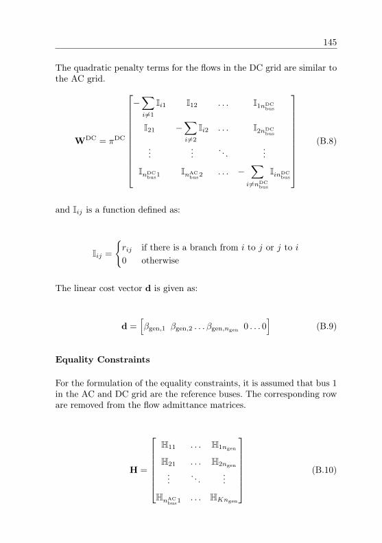
145
The quadratic penalty terms for the flows in the DC grid are similar tothe AC grid.
WDC = πDC
−∑i6=1
Ii1 I12 . . . I1nDCbus
I21 −∑i6=2
Ii2 . . . I2nDCbus
......
. . ....
InDCbus1
InACbus2
. . . −∑i6=nDC
bus
IinDCbus
(B.8)
and Iij is a function defined as:
Iij =
rij if there is a branch from i to j or j to i0 otherwise
The linear cost vector d is given as:
d =[βgen,1 βgen,2 . . . βgen,ngen 0 . . . 0
](B.9)
Equality Constraints
For the formulation of the equality constraints, it is assumed that bus 1in the AC and DC grid are the reference buses. The corresponding roware removed from the flow admittance matrices.
H =
H11 . . . H1ngen
H21 . . . H2ngen
.... . .
...
HnACbus1
. . . HKngen
(B.10)
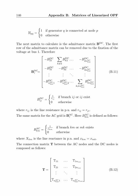
146 Appendix B. Matrices of Linearized OPF
Hpq =
1 if generator q is connected at node p0 otherwise
The next matrix to calculate is the admittance matrix BDC. The firstrow of the admittance matrix can be removed due to the fixation of thevoltage at bus 1. Therefore
BDCr =
−BDC21
∑k 6=2
BDCk2 . . . −BDC
2nACbus
−BDC31 −BDC
32 . . . −BDC3nAC
bus...
.... . .
...
−BDCnDC
bus1−BDC
nDCbus2
. . .∑
k 6=nDCbus
BDCknDC
bus
(B.11)
BDCij =
1rij
if branch ij or ij exist0 otherwise
where rij is the line resistance in p.u. and rij = rji.
The same matrix for the AC grid is BACr . Here BAC
km is defined as follows:
BACkm =
1
xkmif branch km or mk exists
0 otherwise
where Xkm is the line reactance in p.u. and xkm = xmk.
The connection matrix T between the AC nodes and the DC nodes iscomposed as follows:
T =
T11 . . . T1nvsc
T21 . . . T2nvsc
.... . .
...
TnACbus1
. . . TnACbusnvsc
(B.12)

147
Tpq =
1 if terminal q is connected at node p0 otherwise
The same is done for the DC nodes.
S =
S11 . . . S1nvsc
S21 . . . S2nvsc
.... . .
...
SnDCbus1
. . . SnDCbusnvsc
(B.13)
Spq =
−1 if terminal q is connected at DC node p0 otherwise
The equality constraint matrix Ceq can be built out of the alreadydefined matrices.
Ceq =
−BAC 0 HAC T
0 −BDC HDC S
(B.14)
beq = pload (B.15)
The first row corresponds to the power balances at the AC nodes, thesecond row is the respective equations in the DC grid. The equalityvector beq consists out of the total load at each node, for AC and DCnodes.
beq =[p1 p2 . . . p(nAC
bus+nDCbus)
]T(B.16)
Loads can be connected directly to the DC grid, if no such connectionsexist pnvsc,i = 0 for all i > nAC
bus. The inequality constraints are repre-sented by the Ciq matrix. Ingen and Invsc are identity matrices with thesize of ngen and nvsc respectively.

148 Appendix B. Matrices of Linearized OPF
Inequality Constraints
The line adjacency matrix A defines the branches. For each branch thestarting bus is marked with the positive conductivity and the endingbus with the negative. Again the first column can be neglected.
ADCr =
J21 . . . JnDC
bus1
J22 . . . JnDCbus2
.... . .
...
J2nDClin
. . . JnDCbusn
DClin
(B.17)
Jpq =
BDCp if line p starts at node q−BDC
p if line p ends at node q0 otherwise
The same procedure applies for the AC grid results in the AAC matrix,with the size of nAC
bus × nACline.
To limit the DC voltage difference in the grid, matrix L has to bedefined. It just calculates the difference between all terminal voltages.
L =
1 −1 0 0 . . . 0
−1 1 0 0 . . . 0
1 0 −1 0 . . . 0
−1 0 1 0 . . . 0
.... . . . . .
...
0 0 0 . . . 1 −1
0 0 0 . . . −1 1
(B.18)
Combining all matrices together, results in the inequality matrix.

149
Ciq =
AAC 0 0 0
−AAC 0 0 0
0 ADC 0 0
0 −ADC 0 0
0 0 Ingen 0
0 0 −Ingen 0
0 0 0 Invsc
0 0 0 −Invsc
0 L 0 0
(B.19)
The first two rows correspond to the generators limits, followed by tworows for the AC line limits. The transfer capacities of the terminal arelimited in rows 5 and 6. The last two rows limit the flow through theDC lines. The vector biq consists of eight other vectors. There bmax
gen andbmax
gen stand for the upper and lower limits of the generators. bACline and
bDClin represent the line limits for the AC and DC lines, respectively. The
active power through each terminal is limited by the values in bvsc.
bmaxgen =
[pmaxG1 pmax
G2 . . . pmaxGngen
]T(B.20)
bmingen =
[pminG1 pmin
G2 . . . pminGngen
]T(B.21)
bAClin =
[pAClin1 pAC
lin2 . . . pAClinnAC
line
]T(B.22)
bvsc =[pT1 pT2 . . . pTnvsc
]T(B.23)
bDClin =
[pDClin1 pDC
lin2 . . . pDClinnDC
lin
]T(B.24)
b∆uDC =[∆uDC,max ∆uDC,max . . . ∆uDC,max
]T(B.25)

150 Appendix B. Matrices of Linearized OPF
All this vectors together result in biq.
biq =[bmax
genT − bmin
genT bT
lin − bTlin bT
vsc
− bTvsc bT
DClin − bTDClin bT
∆uDC
]T(B.26)

Appendix C
Study Grid Data
C.1 IEEE14 Bus System Combined withMulti-Terminal HVDC Grid
This section provides the test case data for the IEEE14 bus systemcombined with a five bus MTDC overlay grid.
Table C.1: AC bus data for IEEE14 bus test case.
# pload(p.u.)
qload(p.u.)
pmax,gen(p.u.)
qmin,gen(p.u.)
qmax,gen(p.u.)
uACmin
(p.u.)uACmax
(p.u.)
1 0.0 0.0 332.4 0.0 10.0 0.94 1.06
2 21.7 12.7 140.0 -40.0 50.0 0.94 1.06
3 94.2 19.0 100.0 0.0 40.0 0.94 1.06
4 47.8 -3.9 0.0 0.0 0.0 0.94 1.06
5 7.6 1.6 0.0 0.0 0.0 0.94 1.06
6 11.2 7.5 100.0 -6.0 24.0 0.94 1.06
7 0.0 0.0 0.0 0.0 0.0 0.94 1.06
151

152 Appendix C. Study Grid Data
Table C.1: AC bus data for IEEE14 bus test case continued.
# pload(p.u.)
qload(p.u.)
pmax,gen(p.u.)
qmin,gen(p.u.)
qmax,gen(p.u.)
uACmin
(p.u.)uACmax
(p.u.)
8 0.0 0.0 100.0 -6.0 24.0 0.94 1.06
9 29.5 16.6 0.0 0.0 0.0 0.94 1.06
10 9.0 5.8 0.0 0.0 0.0 0.94 1.06
11 3.5 1.8 0.0 0.0 0.0 0.94 1.06
12 6.1 1.6 0.0 0.0 0.0 0.94 1.06
13 13.5 5.8 0.0 0.0 0.0 0.94 1.06
14 14.9 5.0 0.0 0.0 0.0 0.94 1.06
Table C.2: AC line data for IEEE14 bus test case.
# From To rkm(p.u.)
xkm(p.u.)
bkm(p.u.)
pACmax
(p.u.)
1 1 2 0.019 0.059 0.0528 1.0
2 1 5 0.054 0.223 0.0492 1.0
3 2 3 0.047 0.198 0.0438 1.0
4 2 4 0.058 0.176 0.034 1.0
5 2 5 0.057 0.174 0.0346 1.0
6 3 4 0.067 0.171 0.0128 1.0
7 4 5 0.013 0.042 0 1.0
8 4 7 0.000 0.209 0 1.0
9 4 9 0.000 0.556 0 1.0
10 5 6 0.000 0.252 0 1.0

C.1. IEEE14 Bus System Combined with MTDC Grid 153
Table C.2: AC line data for IEEE14 bus test case continued.
# From To rkm(p.u.)
xkm(p.u.)
bkm(p.u.)
pACmax
(p.u.)
11 6 11 0.095 0.199 0 0.5
12 6 12 0.123 0.256 0 0.5
13 6 13 0.066 0.130 0 0.5
14 7 8 0.000 0.176 0 0.5
15 7 9 0.000 0.110 0 0.5
16 9 10 0.032 0.085 0 0.5
17 9 14 0.127 0.270 0 0.5
18 10 11 0.082 0.192 0 0.5
19 12 13 0.221 0.200 0 0.5
20 13 14 0.171 0.348 0 0.5
Table C.3: DC bus data for five bus MTDC grid.
# ACBus
pACvsc,min
(p.u.)pACvsc,max
(p.u.)qACvsc,min
(p.u.)qACvsc,max
(p.u.)uACmin
(p.u.)uACmax
(p.u.)pgen,max
(p.u.)
1 1 -1.0 1.0 -0.5 0.5 0.94 1.06 0.00
2 3 -1.0 1.0 -0.5 0.5 0.94 1.06 0.00
3 9 -1.0 1.0 -0.5 0.5 0.94 1.06 0.00
4 13 -1.0 1.0 -0.5 0.5 0.94 1.06 0.00
5 0 0.0 0.0 0.0 0.0 0.94 1.06 1.00

154 Appendix C. Study Grid Data
Table C.4: DC line data for five bus MTDC grid.
# From To rij(p.u.)
pDCmax,ij
(p.u.)
1 1 13 0.0038 0.50
2 1 25 0.0025 0.50
3 3 25 0.0038 0.50
4 3 9 0.0032 0.50
5 9 13 0.0051 0.50
6 9 25 0.0051 0.50
7 13 25 0.0051 0.50
Table C.5: Generator cost factors for combined IEEE14 bus test casewith a five bus MTDC grid.
# αgen βgen γgen
1 0 0.043 20.0
2 0 0.250 20.0
3 0 0.010 40.0
4 0 0.010 40.0
5 0 0.010 40.0
6 0 0.010 10.0

C.2. RTS96 Test System Combined with MTDC Grid 155
C.2 RTS96 Test System Combined withMulti-Terminal HVDC Grid
This section provides the test case data for the RTS96 system combinedwith an eight bus MTDC overlay grid.
Table C.6: AC bus data for RTS96 test case.
# pload(p.u.)
qload(p.u.)
pmax,gen(p.u.)
qmin,gen(p.u.)
qmax,gen(p.u.)
uACmin
(p.u.)uACmax
(p.u.)
101 1.2 0.2 1.9 -0.5 0.8 0.94 1.06
102 1.1 0.2 1.9 -0.5 0.8 0.94 1.06
103 2.0 0.4 0.0 0.0 0.0 0.94 1.06
104 0.8 0.1 0.0 0.0 0.0 0.94 1.06
105 0.8 0.1 0.0 0.0 0.0 0.94 1.06
106 1.5 0.3 0.0 0.0 0.0 0.94 1.06
107 1.4 0.3 3.0 0.0 1.8 0.94 1.06
108 1.9 0.3 0.0 0.0 0.0 0.94 1.06
109 1.9 0.4 0.0 0.0 0.0 0.94 1.06
110 2.1 0.4 0.0 0.0 0.0 0.94 1.06
111 0.0 0.0 0.0 0.0 0.0 0.94 1.06
112 0.0 0.0 0.0 0.0 0.0 0.94 1.06
113 2.9 0.5 5.9 0.0 2.4 0.94 1.06
114 2.1 0.4 0.1 -0.5 2.0 0.94 1.06
115 3.5 0.6 2.1 -0.5 1.1 0.94 1.06
116 1.1 0.2 1.6 -0.5 0.8 0.94 1.06
117 0.0 0.0 0.0 0.0 0.0 0.94 1.06
118 0.0 0.7 4.0 -0.5 2.0 0.94 1.06

156 Appendix C. Study Grid Data
Table C.6: AC bus data for RTS96 test case continued.
# pload(p.u.)
qload(p.u.)
pmax,gen(p.u.)
qmin,gen(p.u.)
qmax,gen(p.u.)
uACmin
(p.u.)uACmax
(p.u.)
119 2.0 0.4 0.0 0.0 0.0 0.94 1.06
120 1.4 0.3 0.0 0.0 0.0 0.94 1.06
121 0.0 0.0 4.0 -0.5 2.0 0.94 1.06
122 0.0 0.0 3.0 -0.6 1.0 0.94 1.06
123 0.0 0.0 6.6 -1.3 3.1 0.94 1.06
124 0.0 0.0 0.0 0.0 0.0 0.94 1.06
201 1.0 0.2 1.9 -0.5 0.8 0.94 1.06
202 0.9 0.2 1.9 -0.5 0.8 0.94 1.06
203 1.6 0.4 0.0 0.0 0.0 0.94 1.06
204 0.7 0.1 0.0 0.0 0.0 0.94 1.06
205 0.6 0.1 0.0 0.0 0.0 0.94 1.06
206 1.2 0.3 0.0 0.0 0.0 0.94 1.06
207 1.1 0.3 3.0 0.0 1.8 0.94 1.06
208 1.5 0.3 0.0 0.0 0.0 0.94 1.06
209 1.6 0.4 0.0 0.0 0.0 0.94 1.06
210 1.8 0.4 0.0 0.0 0.0 0.94 1.06
211 0.0 0.0 0.0 0.0 0.0 0.94 1.06
212 0.0 0.0 0.0 0.0 0.0 0.94 1.06
213 2.4 0.5 5.9 0.0 2.4 0.94 1.06
214 1.7 0.4 0.1 -0.5 2.0 0.94 1.06
215 2.9 0.6 2.1 -0.5 1.1 0.94 1.06
216 0.9 0.2 1.6 -0.5 0.8 0.94 1.06

C.2. Case Study Security Constrained OPF 157
Table C.6: AC bus data for RTS96 test case continued.
# pload(p.u.)
qload(p.u.)
pmax,gen(p.u.)
qmin,gen(p.u.)
qmax,gen(p.u.)
uACmin
(p.u.)uACmax
(p.u.)
217 0.0 0.0 0.0 0.0 0.0 0.94 1.06
218 0.0 0.7 4.0 -0.5 2.0 0.94 1.06
219 1.6 0.4 0.0 0.0 0.0 0.94 1.06
220 1.2 0.3 0.0 0.0 0.0 0.94 1.06
221 0.0 0.0 4.0 -0.5 2.0 0.94 1.06
222 0.0 0.0 3.0 -0.6 1.0 0.94 1.06
223 0.0 0.0 6.6 -1.3 3.1 0.94 1.06
224 0.0 0.0 0.0 0.0 0.0 0.94 1.06
301 1.1 0.2 1.9 -0.5 0.8 0.94 1.06
302 1.0 0.2 1.9 -0.5 0.8 0.94 1.06
303 1.8 0.4 0.0 0.0 0.0 0.94 1.06
304 0.7 0.1 0.0 0.0 0.0 0.94 1.06
305 0.7 0.1 0.0 0.0 0.0 0.94 1.06
306 1.4 0.3 0.0 0.0 0.0 0.94 1.06
307 1.3 0.3 3.0 0.0 1.8 0.94 1.06
308 1.7 0.3 0.0 0.0 0.0 0.94 1.06
309 1.8 0.4 0.0 0.0 0.0 0.94 1.06
310 2.0 0.4 0.0 0.0 0.0 0.94 1.06
311 0.0 0.0 0.0 0.0 0.0 0.94 1.06
312 0.0 0.0 0.0 0.0 0.0 0.94 1.06
313 2.6 0.5 5.9 0.0 2.4 0.94 1.06
314 1.9 0.4 0.1 -0.5 2.0 0.94 1.06

158 Appendix C. Study Grid Data
Table C.6: AC bus data for RTS96 test case continued.
# pload(p.u.)
qload(p.u.)
pmax,gen(p.u.)
qmin,gen(p.u.)
qmax,gen(p.u.)
uACmin
(p.u.)uACmax
(p.u.)
315 3.2 0.6 2.1 -0.5 1.1 0.94 1.06
316 1.0 0.2 1.6 -0.5 0.8 0.94 1.06
317 0.0 0.0 0.0 0.0 0.0 0.94 1.06
318 0.0 0.7 4.0 -0.5 2.0 0.94 1.06
319 1.8 0.4 0.0 0.0 0.0 0.94 1.06
320 1.3 0.3 0.0 0.0 0.0 0.94 1.06
321 0.0 0.0 4.0 -0.5 2.0 0.94 1.06
322 0.0 0.0 3.0 -0.6 1.0 0.94 1.06
323 0.0 0.0 6.6 -1.3 3.1 0.94 1.06
324 0.0 0.0 0.0 0.0 0.0 0.94 1.06
Table C.7: AC line data for RTS96 test case.
# From To rkm(p.u.)
xkm(p.u.)
bkm(p.u.)
pACmax
(p.u.)
1 101 102 0.003 0.014 0.461 3.0
2 101 103 0.055 0.211 0.057 1.8
3 101 105 0.022 0.085 0.023 1.8
4 102 104 0.033 0.127 0.034 3.0
5 102 106 0.050 0.192 0.052 3.0
6 103 109 0.031 0.119 0.032 1.8
7 103 124 0.002 0.084 0 3.0
8 104 109 0.027 0.104 0.028 1.8

C.2. Case Study Security Constrained OPF 159
Table C.7: AC line data for RTS96 test case continued.
# From To rkm(p.u.)
xkm(p.u.)
bkm(p.u.)
pACmax
(p.u.)
9 105 110 0.023 0.088 0.024 1.8
10 106 110 0.014 0.061 2.46 1.8
11 107 108 0.016 0.061 0.017 1.8
12 107 203 0.042 0.161 0.044 1.8
13 108 109 0.043 0.165 0.045 1.8
14 108 110 0.043 0.165 0.045 1.8
15 109 111 0.002 0.084 0 3.0
16 109 112 0.002 0.084 0 3.0
17 110 111 0.002 0.084 0 3.0
18 110 112 0.002 0.084 0 3.0
19 111 113 0.006 0.048 0.1 5.0
20 111 114 0.005 0.042 0.088 5.0
21 112 113 0.006 0.048 0.1 5.0
22 112 123 0.012 0.097 0.203 5.0
23 113 123 0.011 0.087 0.182 5.0
24 113 215 0.010 0.075 0.158 5.0
25 114 116 0.005 0.059 0.082 5.0
26 115 116 0.002 0.017 0.036 5.0
27 115 121 0.006 0.049 0.103 5.0
28 115 121 0.006 0.049 0.103 5.0
29 115 124 0.007 0.052 0.109 5.0
30 116 117 0.003 0.026 0.055 5.0

160 Appendix C. Study Grid Data
Table C.7: AC line data for RTS96 test case continued.
# From To rkm(p.u.)
xkm(p.u.)
bkm(p.u.)
pACmax
(p.u.)
31 116 119 0.003 0.023 0.049 5.0
32 117 118 0.002 0.014 0.03 5.0
33 117 122 0.014 0.105 0.221 5.0
34 118 121 0.003 0.026 0.055 5.0
35 118 121 0.003 0.026 0.055 5.0
36 119 120 0.005 0.040 0.083 5.0
37 119 120 0.005 0.040 0.083 5.0
38 120 123 0.003 0.022 0.046 5.0
39 120 123 0.003 0.022 0.046 5.0
40 121 122 0.009 0.068 0.142 5.0
41 123 217 0.010 0.074 0.155 5.0
42 201 202 0.003 0.014 0.461 3.0
43 201 203 0.055 0.211 0.057 1.8
44 201 205 0.022 0.085 0.023 1.8
45 202 204 0.033 0.127 0.034 3.0
46 202 206 0.050 0.192 0.052 3.0
47 203 209 0.031 0.119 0.032 1.8
48 203 224 0.002 0.084 0 3.0
49 204 209 0.027 0.104 0.028 1.8
50 205 210 0.023 0.088 0.024 1.8
51 206 210 0.014 0.061 2.46 1.8
52 207 208 0.016 0.061 0.017 1.8

C.2. Case Study Security Constrained OPF 161
Table C.7: AC line data for RTS96 test case continued.
# From To rkm(p.u.)
xkm(p.u.)
bkm(p.u.)
pACmax
(p.u.)
53 208 209 0.043 0.165 0.045 1.8
54 208 210 0.043 0.165 0.045 1.8
55 209 211 0.002 0.084 0 3.0
56 209 212 0.002 0.084 0 3.0
57 210 211 0.002 0.084 0 3.0
58 210 212 0.002 0.084 0 3.0
59 211 213 0.006 0.048 0.1 5.0
60 211 214 0.005 0.042 0.088 5.0
61 212 213 0.006 0.048 0.1 5.0
62 212 223 0.012 0.097 0.203 5.0
63 213 223 0.011 0.087 0.182 5.0
64 214 216 0.005 0.059 0.082 5.0
65 215 216 0.002 0.017 0.036 5.0
66 215 221 0.006 0.049 0.103 5.0
67 215 221 0.006 0.049 0.103 5.0
68 215 224 0.007 0.052 0.109 5.0
69 216 217 0.003 0.026 0.055 5.0
70 216 219 0.003 0.023 0.049 5.0
71 217 218 0.002 0.014 0.03 5.0
72 217 222 0.014 0.105 0.221 5.0
73 218 221 0.003 0.026 0.055 5.0
74 218 221 0.003 0.026 0.055 5.0

162 Appendix C. Study Grid Data
Table C.7: AC line data for RTS96 test case continued.
# From To rkm(p.u.)
xkm(p.u.)
bkm(p.u.)
pACmax
(p.u.)
75 219 220 0.005 0.040 0.083 5.0
76 219 220 0.005 0.040 0.083 5.0
77 220 223 0.003 0.022 0.046 5.0
78 220 223 0.003 0.022 0.046 5.0
79 221 222 0.009 0.068 0.142 5.0
80 301 302 0.003 0.014 0.461 3.0
81 301 303 0.055 0.211 0.057 1.8
82 301 305 0.022 0.085 0.023 1.8
83 302 304 0.033 0.127 0.034 3.0
84 302 306 0.050 0.192 0.052 3.0
85 303 309 0.031 0.119 0.032 1.8
86 303 324 0.002 0.084 0 3.0
87 304 309 0.027 0.104 0.028 1.8
88 305 310 0.023 0.088 0.024 1.8
89 306 310 0.014 0.061 2.46 1.8
90 307 308 0.016 0.061 0.017 1.8
91 308 309 0.043 0.165 0.045 1.8
92 308 310 0.043 0.165 0.045 1.8
93 309 311 0.002 0.084 0 3.0
94 309 312 0.002 0.084 0 3.0
95 310 311 0.002 0.084 0 3.0
96 310 312 0.002 0.084 0 3.0

C.2. Case Study Security Constrained OPF 163
Table C.7: AC line data for RTS96 test case continued.
# From To rkm(p.u.)
xkm(p.u.)
bkm(p.u.)
pACmax
(p.u.)
97 311 313 0.006 0.048 0.1 5.0
98 311 314 0.005 0.042 0.088 5.0
99 312 313 0.006 0.048 0.1 5.0
100 312 323 0.012 0.097 0.203 5.0
101 313 323 0.011 0.087 0.182 5.0
102 314 316 0.005 0.059 0.082 5.0
103 315 316 0.002 0.017 0.036 5.0
104 315 321 0.006 0.049 0.103 5.0
105 315 321 0.006 0.049 0.103 5.0
106 315 324 0.007 0.052 0.109 5.0
107 316 317 0.003 0.026 0.055 5.0
108 316 319 0.003 0.023 0.049 5.0
109 317 318 0.002 0.014 0.03 5.0
110 317 322 0.014 0.105 0.221 5.0
111 318 321 0.003 0.026 0.055 5.0
112 318 321 0.003 0.026 0.055 5.0
113 319 320 0.005 0.040 0.083 5.0
114 319 320 0.005 0.040 0.083 5.0
115 320 323 0.003 0.022 0.046 5.0
116 320 323 0.003 0.022 0.046 5.0
117 321 322 0.009 0.068 0.142 5.0
118 325 121 0.012 0.097 0.203 5.0

164 Appendix C. Study Grid Data
Table C.7: AC line data for RTS96 test case continued.
# From To rkm(p.u.)
xkm(p.u.)
bkm(p.u.)
pACmax
(p.u.)
119 318 223 0.013 0.104 0.218 5.0
120 323 325 0.000 0.009 0 7.2
Table C.8: DC bus data for eight bus MTDC grid.
# ACBus
pACvsc,min
(p.u.)pACvsc,max
(p.u.)qACvsc,min
(p.u.)qACvsc,max
(p.u.)uACmin
(p.u.)uACmax
(p.u.)pgen,max
(p.u.)
1 102 -6.0 6.0 -1.5 1.5 0.94 1.06 0.00
2 121 -6.0 6.0 -1.5 1.5 0.94 1.06 0.00
3 202 -6.0 6.0 -1.5 1.5 0.94 1.06 0.00
4 221 -6.0 6.0 -1.5 1.5 0.94 1.06 0.00
5 302 -6.0 6.0 -1.5 1.5 0.94 1.06 0.00
6 321 -6.0 6.0 -1.5 1.5 0.94 1.06 0.00
7 0 0.0 0.0 0.0 0.0 0.94 1.06 5.00
8 0 0.0 0.0 0.0 0.0 0.94 1.06 4.00
Table C.9: DC line data for eight bus MTDC grid.
# From To rij(p.u.)
pDCmax,ij
(p.u.)
1 102 121 0.0262 2.50
2 102 202 0.1048 2.50
3 102 7 0.0655 2.50

C.2. Case Study Security Constrained OPF 165
Table C.9: DC line data for eight bus MTDC grid continued.
# From To rij(p.u.)
pDCmax,ij
(p.u.)
4 121 221 0.0786 2.50
5 121 321 0.1310 2.50
6 121 7 0.0655 2.50
7 202 221 0.0262 2.50
8 202 302 0.0917 2.50
9 202 7 0.0655 2.50
10 202 8 0.0655 2.50
11 221 321 0.0917 2.50
12 221 7 0.0655 2.50
13 221 8 0.0655 2.50
14 302 321 0.0262 2.50
15 302 8 0.0655 2.50
16 321 8 0.0655 2.50
Table C.10: Generator cost factors for combined RTS96 test case witha five bus MTDC grid.
# αgen βgen γgen
1 0 0.007 73.0
2 0 0.007 73.0
3 0 0.053 43.7
4 0 0.007 48.6
5 0 0.100 100.0

166 Appendix C. Study Grid Data
Table C.10: Generator cost factors for combined RTS96 test case witha five bus MTDC grid continued.
# αgen βgen γgen
6 0 0.275 49.2
7 0 0.008 12.4
8 0 0.000 4.4
9 0 0.000 4.4
10 0 0.001 0.0
11 0 0.007 12.2
12 0 0.007 73.0
13 0 0.007 73.0
14 0 0.053 43.7
15 0 0.007 48.6
16 0 0.100 100.0
17 0 0.275 49.2
18 0 0.008 12.4
19 0 0.000 4.4
20 0 0.000 4.4
21 0 0.000 0.0
22 0 0.007 12.2
23 0 0.007 73.0
24 0 0.007 73.0
25 0 0.053 43.7
26 0 0.007 48.6
27 0 0.100 100.0

C.2. Case Study Security Constrained OPF 167
Table C.10: Generator cost factors for combined RTS96 test case witha five bus MTDC grid continued.
# αgen βgen γgen
28 0 0.275 49.2
29 0 0.008 12.4
30 0 0.000 4.4
31 0 0.000 4.4
32 0 0.001 0.0
33 0 0.007 12.2
34 0 0.010 0.0
35 0 0.010 0.0

168 Appendix C. Study Grid Data
C.3 Dynamic Grid Data
The following tables define the dynamic grid data. All other parametersfor the IEEE14 bus grids, are the same in Table C.1.
Table C.11: DC grid parameter for dynamic simulations.
# From To Length(km)
Resistance(Ω)
Inductance(mH)
Capacitance(µF)
1 1 2 400 0.12 0.0005 0.0043
2 1 3 400 0.12 0.0005 0.0043
3 2 3 600 0.17 0.0008 0.0065
4 2 4 400 0.12 0.0005 0.0043
5 2 5 500 0.14 0.0006 0.0054
6 2 6 1,000 0.29 0.0013 0.0108
7 3 4 400 0.12 0.0005 0.0043
8 3 5 1,000 0.29 0.0013 0.0108
9 4 5 500 0.14 0.0006 0.0054
10 5 6 1,000 0.29 0.0013 0.0108

C.3. Dynamic Grid Data 169
Table C.12: DC bus capacity for dynamic simulations.
# Capacitance (µF)
1 0.0088
2 0.0314
3 0.0260
4 0.0142
5 0.0325
6 0.0217
Table C.13: Generator data for all generators, part 1.
Ra Xl Xd Xq Xd1 Xq1 Xd2 Xq2
0.0025 0.2 1.8 1.7 0.3 0.55 0.25 0.25
Table C.14: Generator data for all generators, part 2.
Td1 Tq1 Td2 Xq2 H KD
8.0 0.4 0.03 0.05 6.5 0


Bibliography
[1] “Ten Year Network Development Plan 2014,” Entso-E, Tech. Rep.,2014.
[2] R. J. Campbell, “Weather-Related Power Outages and ElectricSystem Resiliency,” Congressional Research Service Report, vol.August 28, no. R42696, pp. 1–15, 2012. [Online]. Available:http://www.fas.org/sgp/crs/misc/R42696.pdf
[3] T. Adm and S. Etu, “Energy Infrastructure Costs and Investmentsbetween 1996 and 2013 (medium-term) and further to 2023 (long-term) on the Trans-European Energy Network and its Connectionto Neighbouring Regions with emphasis on investments on renew-able energy sources and their integration into the Trans-Europeanenergy networks, including an Inventory of the Technical Statusof the European Energy-Network for the Year 2003,” CESI spa,Italy, IIT, Spain, ME, Spain Ramboll A/S, Denmark, Tech. Rep.October, 2005.
[4] P. Fairley, “DC Versus AC: The Second War of Cur-rents Has Already Begun [In My View],” IEEE Powerand Energy Magazine, vol. 10, no. 6, pp. 104–103, nov2012. [Online]. Available: http://ieeexplore.ieee.org/lpdocs/epic03/wrapper.htm?arnumber=6331742
[5] B. O. N. Hansson, “Submarine Cable for 100-kv D-C PowerTransmission,” Electrical Engineering, vol. 73, no. 7, pp. 602–602,jul 1954. [Online]. Available: http://ieeexplore.ieee.org/lpdocs/epic03/wrapper.htm?arnumber=6438864
171

172 Bibliography
[6] R. Koropatnick, “HVDC Project Listing,” HVDC and FlexibleAC Transmission Subcommitee, Tech. Rep. March, 2012. [On-line]. Available: http://www.ece.uidaho.edu/hvdcfacts/Projects/HVDCProjectsListingMarch2012-existing.pdf
[7] Deutsche Gesellschaft Club of Rome, “The Trans-MediterraneanRenewable Energy Cooperation, Network of Scientists and En-gineers around the Mediterranean Solar Mediterranean Union -Way to Energy and Climate Security?” Press release by TREC,2008.
[8] F. Zickfeld and A. Wieland, “Desert Power 2050: Perspectives ona Sustainable Power System for EUMENA,” Dii GmbH, Tech.Rep., 2012. [Online]. Available: http://www.desertenergy.org
[9] Working Group1, “Final Report Working Group 1 - GridConfiguration -Initial Findings,” The North Seas CountriesOffshore Grid Initiative, Tech. Rep. November, 2012. [On-line]. Available: http://www.benelux.int/NSCOGI/NSCOGI_WG1_OffshoreGridReport.pdf
[10] Friends of the Supergrid, “Position Paper on theEC Communication for a European Infrastructure Pack-age,” Friends of the Supergrid, Tech. Rep., 2010. [On-line]. Available: http://mainstream-downloads.opendebate.co.uk/downloads/Supergrid-Phase-1-Final.pdf
[11] D. Woodford, G. Irwin, and K. Epp, “Stage 1 AWC New JerseyEnergy Link,” in IEEE Power and Energy Society General Meet-ing (PES GM), Vancouver, Canada, 2014, pp. 1–6.
[12] R. Marais and K. Leask, “The Need for HVDC Systems in SouthAfrica and the Region R MARAIS K LEASK Eskom SouthAfrica,” in Cigré International Symposium, Lund, Sweden, 2015,pp. 1–10.
[13] M. Vinícius, G. S. Farinha, M. D. Fátima, D. C. Gama, A. R.Branco, C. Rio, and D. J. Rj, “Transmission Expansion PlanningChallenges Associated to Belo Monte Power Plants HVDC Links,”in Cigré International Symposium, Lund, Sweden, 2015.
[14] G. Bathurst and P. Bordignan, “Delivery of the Nanao Multi-terminal VSC-HVDC System,” in Cigré International Symposium,Lund, Sweden, 2015, pp. 1–12.

Bibliography 173
[15] E. Iggland, R. Wiget, S. Chatzivasileiadis, and G. Andersson,“Multi-Area DC-OPF for HVAC and HVDC Grids,” IEEE Trans-actions on Power Systems, vol. 99, pp. 1–10, 2014.
[16] R. Wiget, M. Imhof, M. A. Bucher, and G. Andersson, “Overviewof a Hierarchical Controller Structure for Multi-Terminal HVDCgrids,” in Cigré International Symposium, Lund, Sweden, 2015.
[17] L. Mackay, T. G. Hailu, G. Chandra Mouli, L. Ramirez-Elizondo,J. Ferreira, and P. Bauer, “From DC Nano- and Microgrids To-wards the Universal DC Distribution System - A Plea to ThinkFurther Into the Future,” in Power and Energy Societey GeneralMeeting (PES GM), Denver, CO, 2015.
[18] T. Dragicevic, J. C. Vasquez, J. M. Guerrero, and D. Skrlec, “Ad-vanced LVDC Electrical Power Architectures and Microgrids: Astep toward a new generation of power distribution networks.”IEEE Electrification Magazine, vol. 2, no. 1, pp. 54–65, 2014.
[19] L. Mackay, M. Imhof, R. Wiget, and G. Andersson, “Voltage de-pendent pricing in DC distribution grids,” in IEEE PowerTech,Grenoble, France, 2013, pp. 1–6.
[20] VDE-Ausschuss Geschichte der Elektrotechnik, “AktuellesGeschichte der elektrischen Energietechnik Von Miesbach nachMünchen - die erste Fernübertragung von elektrischem Strom,”Geschichte der elektrischen Energietechnik, 2007. [Online].Available: https://www.vde.com/de/fg/ETG/Arbeitsgebiete/Geschichte/Aktuelles/Seiten/Miesbach-Muenchen.aspx
[21] E. T. Center, “Oskar von Miller - Electrical Pioneer and BusinessLeader,” 2015. [Online]. Available: http://www.edisontechcenter.org/OskarVonMiller.html
[22] G. King, “Edison vs. Westinghouse: A Shocking Rivalry,” Smithso-nian, 2011. [Online]. Available: http://www.smithsonianmag.com
[23] Electrosuisse, “Technology is our business - René Thury,”Pioniere S bis Z, 2011. [Online]. Available: https://www.electrosuisse.ch/fileadmin/user_upload_electrosuisse/Verband/Verlag/Pioniere/Pioniere_S_bis_Z/ThuryR.pdf
[24] J. Arrillaga, Y. Liu, and N. Watson, Flexible Power Transmission- The HVDC Options. John Wiley & Sons Ltd, 2007.

174 Bibliography
[25] M. Milligan, E. Ela, J. Hein, T. Schneider, G. Brinkman, andP. Denholm, “Renewable Electricity Futures Study Bulk ElectricPower Systems : Operations and Transmission Planning,” Na-tional Renewable Energy Laboratory (NREL), USA, Tech. Rep.,2012.
[26] K. Padiyar, HVDC Power Transmission Systems. New Age In-ternational Ltd., 2010.
[27] C.-K. Kim, V. K. Sood, G.-S. Jang, S.-J. Lim, and S.-J. Lee,HVDC Transmission. John Wiley & Sons Ltd, 2009.
[28] D. V. Hertem, M. Ghandhari, and M. Delimar, “Technical Lim-itations Towards a SuperGrid - A European Prospective,” inIEEE International Energy Conference (ENERGYCON), Man-ama, Bahrain, 2010, pp. 302–309.
[29] K. Meah and S. Ula, “Comparative Evaluation of HVDC andHVAC Transmission Systems,” in IEEE Power and Energy So-ciety General Meeting (PES GM), Tampa, FL, 2007, pp. 1–5.
[30] D. Van Hertem and M. Ghandhari, “Multi-Terminal VSC HVDCfor the European Supergrid: Obstacles,” Renewable and Sustain-able Energy Reviews, vol. 14, no. 9, pp. 3156–3163, 2010.
[31] A. Küchler, Hochspannungstechnik. Springer-Verlag Berlin Hei-delberg, 2005.
[32] M. P. Bahrman, “Overview of HVDC Transmission,” in IEEEPower Systems Conference and Exposition (PSCE), Atlanta, GA,2006, pp. 18–23.
[33] Siemens, “Power Engineering Guide, Power Transmission andDistribution Solutions., Edition 7.0,” Siemens, Tech. Rep.,2012. [Online]. Available: http://www.energy.siemens.com/hq/en/energy-topics/publications/power-engineering-guide/
[34] M. Imhof, O. Valgaev, and G. Andersson, “Controlled IslandingUsing VSC-HVDC Links to Reduce Load Shedding,” in IEEEPowerTech, Eindhoven, Netherlands, 2015.
[35] V. K. Sood, HVDC and FACTS Controllers. Kluwer AcademicPublisher, 2004.

Bibliography 175
[36] G. Persson, “HVDC Converter Operations and Performance, Clas-sic and VSC,” Dhaka, 2011.
[37] D. Jovcic and K. Ahmed, High Voltage Direct Current Transmis-sion: Converters, Systems and DC Grids. Wiley, 2015.
[38] A. M. Isaac and K. Rathi, “Performance Analysis of HybridHVDC Transmission Systems for Connecting Offshore Wind Farmto Onshore Grid,” International Journal of Innovative Reseach inScience, Engineering and Technology, vol. 3, no. 5, pp. 201–207,2014.
[39] A.-K. Marten and D. Westermann, “Local HVDC Grid Opera-tion with Multiple TSO Coordination at a Global Optimum,”in 2014 IEEE International Energy Conference (ENERGYCON),Dubrovnik, Croatia, 2014, pp. 1549–1553.
[40] M. Andreasson, R. Wiget, D. V. Dimarogonas, and K. H. Jo-hansson, “Distributed Primary Frequency Control through Multi-Terminal HVDC Transmission Systems,” in American ControlConference (ACC), Chicago, IL, 2015.
[41] A. Yazdani and R. Iravani, Voltage-Sourced Converters in PowerSystems. John Wiley & Sons Ltd, 2010.
[42] R. Wiget and G. Andersson, “Optimal Power Flow for CombinedAC and Multi-Terminal HVDC Grids Based on VSC Converters,”in IEEE Power and Energy Society General Meeting (PES GM),San Diego, CA, 2012.
[43] ——, “DC Optimal Power Flow Including HVDC Grids,” in IEEEElectrical Power and Energy Conference (EPEC), no. 3, Halifax,Canada, 2013, pp. 1–6.
[44] E. E. George, “Intrasystem Transmission Losses,” Transactions ofthe American Institute of Electrical Engineers, vol. 62, no. 3, 1943.
[45] J. F. Calvert, “Minimization in Electric Systems,” in AIEE FallGeneral Meeting, Chicago, IL, 1957, pp. 1439–1446.
[46] H. Dommel and W. Tinney, “Optimal Power Flow Solutions,”IEEE Transactions on Power Apparatus and Systems, vol. PAS-87, no. 10, pp. 1866–1876, 1968.

176 Bibliography
[47] R. Burchett, H. Happ, and K. Wirgau, “Large Scale OptimalPower Flow,” IEEE Transactions on Power Apparatus and Sys-tems, vol. PAS-101, no. 10, pp. 3722–3732, 1982.
[48] R. Burchett, H. Happ, D. Vierath, and K. Wirgau, “Developmentsin Optimal Power Flow,” IEEE Transactions on Power Apparatusand Systems, vol. PAS-101, no. 2, pp. 406–414, 1982.
[49] M. Huneault and F. D. Galiana, “A Survey of the Optimal PowerFlow Literature,” IEEE Transactions on Power Systems, vol. 6,no. 2, pp. 762–770, 1991.
[50] K. S. Pandya and S. K. Joshi, “A Survey of Optimal Power FlowMethods,” Journal of Applied Information Technology, vol. 4,no. 5, pp. 450–458, 2005.
[51] S. Frank, I. Steponavice, and S. Rebennack, “Optimal Power Flow:A Bibliographic Survey II Non-deterministic and Hybrid Meth-ods,” in Energy Systems. Springer-Verlag Berlin Heidelberg, 2012,vol. 3, no. 3, pp. 259–289.
[52] P. M. Pardalos, Handbook of Power Systems II. Springer-VerlagBerlin Heidelberg, 2010.
[53] L. G. L. Gengyin, Z. M. Z. Ming, H. J. H. Jie, L. G. L. Guangkai,and L. H. L. Haifeng, “Power Flow Calculation of Power Sys-tems Incorporating VSC-HVDC,” in International Conference onPower System Technology (PowerCon), vol. 2, no. November, Sin-gapore, Singapore, 2004, pp. 21–24.
[54] A. Pizano-Martinez, C. R. Fuerte-Esquivel, H. Ambriz-Pérez, andE. Acha, “Modeling of VSC-based HVDC Systems for a Newton-Raphson OPF Algorithm,” IEEE Transactions on Power Systems,vol. 22, no. 4, pp. 1794–1803, 2007.
[55] X. P. Zhang, “Multiterminal Voltage-Sourced Converter-BasedHVDC Models for Power Flow Analysis,” IEEE Transactions onPower Systems, vol. 19, no. 4, pp. 1877–1884, 2004.
[56] J. Beerten, S. Cole, and R. Belmans, “A Sequential AC/DC PowerFlow Algorithm for Networks Containing Multi-Terminal VSCHVDC Systems,” in IEEE Power and Energy Society GeneralMeeting (PES GM), Minesota, MM, 2010, pp. 1–7.

Bibliography 177
[57] G. Andersson, “Modelling and Analysis of Electric Power Sys-tems,” Lecture Notes - ETH Zürich, 2012.
[58] P. Kundur, Power System Stability and Control. McGraw-Hill,Inc, 1994.
[59] A. Monticelli, State Estimation in Electric Power Systems.Boston, MA: Springer US, 1999.
[60] O. Heyman, “HVDC Light - It’s time to connect,” ABB AB GridSystems - HVDC, Tech. Rep., 2012.
[61] A. Lesnicar and R. Marquardt, “An Innovative Modular MultilevelConverter Topology Suitable for a Wide Power Range,” in IEEEPowerTech, vol. 3, Bologna, Italy, 2003, pp. 272–277.
[62] G. Daelemans, K. Srivastava, M. Reza, S. Cole, and R. Belmans,“Minimization of Steady-State Losses in Meshed Networks usingVSC HVDC,” in IEEE Power and Energy Society General Meeting(PES GM), Calgary, Canada, 2009, pp. 1–5.
[63] H. Pang, G. Tang, and Z. He, “Evaluation of Losses in VSC-HVDCTransmission System,” in IEEE Power and Energy Society Gen-eral Meeting (PES GM), Pittsburg, PA, 2008, pp. 1–6.
[64] P. S. Jones and C. C. Davidson, “Calculation of Power Losses forMMC-Based VSC HVDC Stations,” in 5th European Conferenceon Power Electronics and Applications (EPE), no. Mmc, Lille,France, 2013.
[65] W. Feng, S. Member, L. A. Tuan, L. B. Tjernberg, S. Member,A. Mannikoff, and A. Bergman, “A New Approach for BenefitEvaluation of Multiterminal VSC - HVDC Using A ProposedMixed AC / DC Optimal Power Flow,” IEEE Transactions onPower Delivery, vol. 29, no. 1, pp. 432–443, 2014.
[66] A.-K. Marten, F. Sass, and D. Westermann, “Mixed AC/DC OPFusing Differential Evolution for Global Minima Identification,” inPowerTech, Eindhoven, Netherlands, 2015, pp. 1–6.
[67] B. Stott, J. Jardim, and O. Alsac, “DC Power Flow Revisited,”IEEE Transactions on Power Systems, vol. 24, no. 3, pp. 1290–1300, 2009.
178 Bibliography
[68] W. Hahn, “Load Studies on the D-C Calculating Table,” GeneralElectric Review. Schenectady NY, vol. 34, pp. 444–45, 1931.
[69] J. A. Casazza and W. S. Ku, “The Coordinated use of A-C andD-C Network Analyzers,” in American Power Conference, Vol. 16,1954.
[70] J. Beerten, S. Cole, and R. Belmans, “A Sequential AC/DC PowerFlow Algorithm for Networks Containing Multi-Terminal VSCHVDC Systems,” in IEEE Power and Energy Society GeneralMeeting (PES GM), Detroit, MI, jul 2010, pp. 1–7.
[71] R. D. Christie, “Power Systems Test Case Archive -UWEE,” 1999. [Online]. Available: https://www.ee.washington.edu/research/pstca/
[72] R. Wiget and E. Iggland, “Security Constrained Optimal PowerFlow for HVAC and HVDC Grids,” in Power Systems Computa-tion Conference (PSCC), Wroclaw, Poland, 2014.
[73] V. Saplamidis and R. Wiget, “Security Constrained OptimalPower Flow for Mixed AC and Multi-Terminal HVDC Grids,”in PowerTech, Eindhoven, Netherlands, 2015.
[74] O. Alsac and B. Stott, “Optimal Load Flow with Steady-StateSecurity,” IEEE Transactions on Power Apparatus and Systems,vol. PAS-93, no. 3, pp. 745–751, 1974.
[75] “Network Code on Operational Security,” Entso-E, Tech. Rep.September, 2013.
[76] R. Wiget and M. Vrakopoulou, “Probabilistic Security Con-strained Optimal Power Flow for a Mixed HVAC and HVDC Gridwith Stochastic Infeed,” in Power Systems Computation Confer-ence (PSCC), Wroclaw, Poland, 2014.
[77] D. Gan, R. Thomas, and R. Zimmerman, “Stability-ConstrainedOptimal Power Flow,” IEEE Transactions on Power Systems,vol. 15, no. 2, pp. 535–540, 2000.
[78] F. Capitanescu, J. L. Martinez Ramos, P. Panciatici, D. Kirschen,A. Marano Marcolini, L. Platbrood, and L. Wehenkel, “State-of-the-Art, Challenges, and Future Trends in Security ConstrainedOptimal Power Flow,” Electric Power Systems Research, vol. 81,no. 8, pp. 1731–1741, 2011.

Bibliography 179
[79] P. Sauer, K. Reinhard, and T. Overbye, “Extended Factors forLinear Contingency Analysis,” in Annual Hawaii InternationalConference on System Sciences, Wailea Alanui, HI, 2001, pp. 1–7.
[80] A. J. Wood and B. F. Wollenberg, Power Generation Operationand Control, 2nd ed. John Wiley & Sons Ltd, 1996.
[81] K. Holmstr, O. G. Anders, and M. M. Edvall, “User ’ S Guide forTomlab / Minos 1,” Options, pp. 1–114, 2008.
[82] C. Grigg, P. Wong, P. Albrecht, R. Allan, M. Bhavaraju,R. Billinton, Q. Chen, C. Fong, S. Haddad, S. Kuruganty,W. Li, R. Mukerji, D. Patton, N. Rau, D. Reppen, A. Schnei-der, M. Shahidehpour, and C. Singh, “The IEEE Reliability TestSystem-1996. A Report Prepared by the Reliability Test SystemTask Force of the Application of Probability Methods Subcom-mittee,” IEEE Transactions on Power Systems, vol. 14, no. 3, pp.1010–1020, 1999.
[83] R. D. Christie, “Power Systems Test Case Archive - ReliabilityTest System (RTS) - 1996,” 1996. [Online]. Available: https://www.ee.washington.edu/research/pstca/rts/pg_tcarts.htm
[84] ——, “Power Systems Test Case Archive - 14 Bus PowerFlow Test Case,” 1993. [Online]. Available: https://www.ee.washington.edu/research/pstca/pf14/pg_tca14bus.htm
[85] R. D. Zimmerman, C. E. Murillo-Sanchez, and R. J. Thomas,“MATPOWER: Steady-State Operations, Planning, and AnalysisTools for Power Systems Research and Education,” IEEE Trans-actions on Power Systems, vol. 26, no. 1, pp. 12–19, feb 2011.
[86] N. MacLeod, “A Technological Roadmap for the Development ofthe European Supergrid - Questions,” Lund, Sweden, 2015.
[87] Nordic Operations Development Group (NOD), “Evaluation ofthe Ramping Restriction in the Energy Market,” Entso-E, Tech.Rep. November, 2010.
[88] K. Frey, K. Rudion, and J. Christian, “Optimal Operation Strat-egy for VSC HVDC Links within an Interconnected Power Sys-tem,” in Cigré International Symposium, Lund, Sweden, 2015.

180 Bibliography
[89] R. Wiget, M. Andreasson, G. Andersson, K. H. Johansson, andD. V. Dimarogonas, “Dynamic Simulation of a Combined AC andMTDC Grid with Decentralized Controllers to Share Primary Fre-quency Control Reserves,” in PowerTech, Eindhoven, Netherlands,2015.
[90] M. Andreasson, R. Wiget, D. V. Dimarogonas, and K. H. Johans-son, “Distributed Secondary Frequency Control through MTDCTransmission Systems,” in IEEE Conference ond Decision andControl (CDC), Osaka, Japan, 2015.
[91] ——, “Coordinated Frequency Control through MTDC Trans-mission Systems,” in Distributed Estimation and Control in Net-worked Systems (Necsys), Philadelphia, PA, 2015, pp. 1–6.
[92] M. Andreasson, “Distributed control of networked dynamical sys-tems and electrical power systems (preliminary title),” PhD The-sis, KTH, Stockholm, 2016.
[93] R. Li, S. Bozhko, and G. Asher, “Frequency Control Design forOffshore Wind Farm Grid with LCC-HVDC Link Connection,”IEEE Transactions on Power Electronics, vol. 23, no. 3, pp. 1085–1092, 2008.
[94] L. Fan, Z. Miao, and D. Osborn, “Wind Farms with HVDC De-livery in Load Frequency Control,” IEEE Transactions on PowerSystems, vol. 24, no. 4, pp. 1894–1895, 2009.
[95] U. Axelsson, “The Gotland HVDC Light Project - Experiencesfrom Trial and Commercial Operation,” in 16th InternationalConference and Exhibition on Electricity Distribution (CIRED),Amsterdam, Netherlands, 2001.
[96] J. Dai and G. Damm, “An Improved Law Using HVDC Systemsfor Frequency Control,” in Power Systems Computation Confer-ence (PSCC), Stockholm, Sweden, 2011, pp. 4–9.
[97] M. Andreasson, M. Nazari, D. V. Dimarogonas, H. Sandberg,K. H. Johansson, M. Ghandhari, and E. P. Systems, “DistributedVoltage and Current Control of Multi-Terminal High-Voltage Di-rect Current Transmission Systems,” in 19th World Congress ofthe International Federation of Automatic Control (IFAC), CapeTown, South Africa, 2014.

Bibliography 181
[98] M. Andreasson, D. V. Dimarogonas, H. Sandberg, and K. H. Jo-hansson, “Control of MTDC Transmission Systems under LocalInformation,” in Conference of Decision and Control (CDC), LosAngeles, CA, 2014.
[99] J. Dai, Y. Phulpin, A. Sarlette, and D. Ernst, “Impact of Delayson a Consensus-Based Primary Frequency Control Scheme for ACSystems Connected by a Multi-Terminal HVDC Grid,” in IREPSymposium - Bulk Power System Dynamics and Control - VIII,Rio de Janeiro, Brazil, 2010.
[100] B. Silva, C. L. Moreira, L. Seca, Y. Phulpin, and J. A. P. Lopes,“Provision of Inertial and Primary Frequency Control Services us-ing Offshore Multiterminal HVDC Networks,” IEEE Transactionson Sustainable Energy, vol. 3, no. 4, pp. 800–808, 2012.
[101] D. Jing, Y. Phulpin, A. Sarlette, and D. Ernst, “Voltage Controlin an HVDC System to Share Primary Frequency Reserves Be-tween Non-Synchronous Areas,” in Power Systems ComputationConference (PSCC), Stockholm, Sweden, 2011.
[102] J. A. Taylor and L. Scardovi, “Decentralized Control of DC-Segmented Power Systems,” in 52nd Annual Allerton Conferenceon Communication, Control, and Computing (Allerton), Urbana,IL, 2014, pp. 1046–1050.
[103] M. Andreasson, R. Wiget, D. V. Dimarogonas, K. H. Johans-son, and G. Andersson, “Coordinated Frequency Control throughMTDC Transmission Systems,” submitted (2nd round of revision)to IEEE Transactions on Power Systems, 2015.
[104] N. Jaleeli, L. VanSlyck, D. Ewart, L. Fink, and a.G. Hoffmann,“Understanding automatic generation control,” IEEE Transac-tions on Power Systems, vol. 7, no. 3, pp. 1106–1122, 1992.
[105] T. H. Demiray, “Simulation of Power System Dynamic using Dy-namic Phasor Models,” PhD Thesis, ETH Zürich, 2008.
[106] M. Imhof, “Voltage Source Converter Based HVDC – Modellingand Coordinated Control to Enhance Power System Stability,”PhD Thesis, ETH Zürich, 2015.

182 Bibliography
[107] T. Haase, “Anforderungen an eine durch Erneuerbare Energiengeprägte Energieversorgung - Untersuchung des Regelverhaltensvon Kraftwerken und Verbundnetzen,” PhD Thesis, UniversitätRostock, 2006.
[108] S. H. Low, “Convex Relaxation of Optimal Power Flow - Part I:Formulations and Equivalence,” IEEE Transactions on Control ofNetwork Systems, vol. 1, no. 1, pp. 15–27, mar 2014.
[109] ——, “Convex Relaxation of Optimal Power Flow - Part II: Exact-ness,” IEEE Transactions on Control of Network Systems, vol. 1,no. 2, pp. 177–189, jun 2014.
[110] M. K. Bucher, R. Wiget, G. Andersson, and C. M. Franck, “Mul-titerminal HVDC Networks - What is the Preferred Topology,”IEEE Transactions on Power Delivery, vol. 29, no. 1, pp. 406–413, 2014.
[111] M. A. Bucher, R. Wiget, G. H.-B. Perez, and G. Andersson, “Op-timal placement of multi-terminal HVDC interconnections for in-creased operational flexibility,” in IEEE PES Innovative SmartGrid Technologies, Europe (ISGT-Europe). Istanbul, Turkey:IEEE, oct 2014, pp. 1–6.