rising wage inequality and human capital investment rising wage inequality and human capital...
TRANSCRIPT
1
Rising Wage Inequality and Human Capital Investment
Lancelot Henry de Frahan & Carolyn M. Sloane1
November 12, 2015
University of Chicago
Abstract:
In this paper, we fill the gap in the existing literature on the causal effects of rising inequality on human
capital investment. First, we propose an instrumentation strategy that yields a vector of instruments
from a predicted local wage distribution by interacting initial industry employment shares at the
metropolitan level with changes to the within-industry distribution of wages at the national level. With
this instrumentation strategy, we are able to separately analyze the causal impact of changing inequality
from changes in mean income on postsecondary enrollments. This paper establishes an empirical fact:
predicted increases in local wage inequality depress rates of enrollment in postsecondary schooling. In
our main analysis on community college enrollments, we find that moving from the 10th to the 90th
percentile of changes in wage inequality corresponds to a 2.05 percentage point decrease in first-year,
full-time aggregate community college enrollments. Further, we find evidence of a causal relationship
between rising local inequality and residential sorting on an income basis which sheds light on a
possible mechanism driving our main result. The instrumentation strategy introduced in this paper
could allow researchers to assess the causal relationship between inequality and other economic
phenomena.
1 Email: [email protected], [email protected]. We are indebted to Marianne Bertrand, Dan Black, Kerwin
Charles, and Erik Hurst for support and guidance throughout this project. We are grateful for comments from Steven Durlauf, Michal Fabinger, Emir Kamenica, Ben Keys, Susan Mayer, Glen Weyl, and Seth Zimmerman. We thank Dan Alexander for collaboration that propelled this project. We thank seminar participants at Chicago Booth, Chicago Harris and the University of Chicago Economics Department for feedback.

2
I. Introduction
This paper analyzes the real effects of rising local wage inequality on human capital investment
and establishes an empirical fact: predicted increases in local wage inequality cause declines in
enrollment rates in both community colleges and four-year institutions. The context of our research
question is a labor market in which returns to workers have become increasingly unequal over the last
30 years. Figure 1 documents trends in wage inequality in the March Current Population Survey (CPS)
from 1980 to 2008.2 Across any measure of dispersion, inequality has been on the rise since 1980. The
Gini coefficient in wages, a measure of overall inequality, increased from 0.34 in 1980 to 0.43 in 2008.
At the upper tail, the difference in log wages between workers at the 90th and 50th percentiles of the
wage distribution, widened from 0.72 in 1980 to 0.84 in 2008. From 1980 to 2008, the difference in
log wages between those with and without four-year college attainment more than doubled from 0.30
in 1980 to 0.68 in 2008.3
The phenomenon of rising wage inequality occupies considerable space in the public forum. In
the policy realm, the declining relative position of the American middle class was a recurrent theme in
every State of the Union address during the Obama presidency, and income inequality has featured as
a topic of debate in the 2016 Presidential primary season. In bestsellers, newspaper columns and blog
posts, economists have directed public attention to the rise in inequality.4 The academic literature has
focused almost exclusively on chronicling the upward trend in wage inequality. Juhn, Murphy, and
Pierce (1993) documents the rise in wage inequality for men in the March CPS. From 1963 to 1989,
real wages for men at the 10th percentile declined by 5 percent whereas real wages for men at the 90th
percentile rose by about 40 percent.5 Autor, Katz, and Kearney (2008) highlights the slowdown in
lower tail inequality growth relative to increases at the upper tail from 1987 to 2005.6 Using
administrative tax data to follow income growth at the top of the income distribution, Piketty and
2 Time series constructed from authors’ calculations from the March CPS 1980-2008 of non-institutional individuals age 21 to 64 with strong attachment to the labor force (work at least 30 hours a week, 48 weeks a year and earn at least $5,000/ year in 2000$). The “90-50” refers to the log difference in wages of workers at the 90th and 50th percentiles of the wage distribution. The “skill premium” refers to the log difference in wages of workers with and without four-year college attainment. 3 Authors’ calculations from the March CPS 1980-2008 in wages of those who are strongly attached to the labor market in real 2000$. 4 See Cochrane (2014), Krugman (2015), Piketty (2014), Stiglitz (2012), and Putnam (2015). 5 See also Katz and Murphy (1992); Murphy and Welch (1992). 6 Using the March CPS the authors show that from 1979 to 1987, the difference in log wages between those at the 90th percentile and those at the 50th percentile (90-50) and those at the 50th percentile and the 10th percentile (50-10) increased. From 1987 there were steep increases in 90-50 persist from 1987 to present, but that growth in lower tail inequality dampens.
3
Saez (2003) establishes a Kuznets U-shaped pattern in the top decile’s income share from 1917 to
1998.7 With respect to well-being, studies such as Aguiar and Bils (2015) have tracked the simultaneous
rise of income and consumption inequality over this period.8
Concurrent to the rise in wage inequality, a compositional change was underway in the US labor
market. A hallmark of the post-War labor market was a rapid accumulation of schooling by workers.
For every birth cohort from 1875 to 1950, college completion increased. However, for birth cohorts
from 1950 to 1965 college completion flattened. This first college attainment slowdown is
documented in Goldin and Katz (2008). Using the March CPS from 1994 to 2014, we show evidence
for a second schooling slowdown. Figure 2 presents trends in predicted postsecondary schooling for
birth cohorts from 1960 to 1990.9 Among men, postsecondary schooling slows for the 1970 to 1981
birth cohorts before increasing again for later cohorts perhaps in response to the Great Recession.
For women, whose schooling rates are higher, the slowdown is less pronounced and shorter in
duration.
The timing of the increasing national trends in wage inequality and the slowdown in college
attainment is suggestive, but not informative, about the potential relationship between inequality and
human capital investment. A natural question arises: what are the causal effects, if any, of rising wage
inequality on human capital investment? Economic theory offers three primary channels through
which we may expect human capital and wage dispersion to be related: (1) by altering incentives to
invest in human capital, (2) through the non-linear impact of income on human capital investment
particularly in the presence of credit constraints, and (3) through inequality’s impact on aggregate
responses such as policy feedback and residential sorting. Each channel offers a unique prediction for
the sign of the gradient of changes in schooling on changes in wage inequality.
We begin by considering the impact of a changing wage distribution on incentives to invest in
human capital. Monetary returns to education depend on the individual’s wage once skill has been
acquired and the individual’s wage in the absence of additional skill.10 In the labor market, a premium
may be offered for worker skill whether that be formal training or experience. As the relative premium
7 Kuznets (1955) posited that trends in income inequality over time would take on a U-shape as a country grows. 8 See also Fisher, Johnson, Smeeding (2012) and Attanasio, Hurst and Pistaferri (2012). 9 Time series constructed from authors’ calculations from the March CPS 1994-2014 of non-institutional individuals age 25-54. We predict any postsecondary schooling separately for men and women by using a linear probability model of any schooling beyond grade 12 on birth year, an age quartic, and normalized year fixed effects where the first and last year effects = 0 following Hall (1968). A distinction from Goldin and Katz (2008) is that our measure of attainment is any postsecondary schooling beyond grade 12 whereas Goldin and Katz track college completion. 10 As noted in Roy (1951), this mark-up is based on a counterfactual and not directly observable. Even so, the current wage distribution likely contains considerable information about the monetary gains from college.

4
paid to skilled labor increases, the incentives to acquire skill intensify and postsecondary schooling
enrollments increase (Katz and Murphy 1992). While standard theories of the skill premium suggest
that increasing inequality may increase schooling propensities, there are other stories that suggest a
negative relationship between inequality and schooling. For example, if inequality results in more
binding liquidity constraints, this may prevent potential students from accumulating human capital
(Carneiro and Heckman 2002). If the poor are more likely to be on the margin of the enrollment decision,
an increase in wage dispersion in the presence of credit constraints may result in aggregate declines in
enrollment. Likewise, inequality may negatively impact human capital accumulation by affecting
neighborhood composition. An increase in inequality may cause changes in residential sorting patterns
based on income which may cause children from lower income households to attend lower quality
schools leaving them ill-prepared for further education (Durlauf 1996). Lastly, theories that tie rising
inequality with policy responses are ambiguous with respect to enrollment effects. If voters demand
more public goods in the face of rising inequality, and human capital production is increasing in the
quantity and quality of public goods, enrollments may increase (Meltzer and Richard 1981). On the
other hand, if increasing inequality provokes political friction this may adversely affect the quality and
quantity of public goods thereby negatively impacting human capital investment (Benabou 1996,
2000). Theoretically the causal impact of rising local wage inequality on aggregate postsecondary
enrollments is uncertain.
To date, there has been little empirical work exploring the causal relationship between recent rising
wage inequality and postsecondary schooling enrollments.11 In this paper, we fill the gap in the existing
literature on the consequences of rising inequality by proposing an instrumentation strategy that yields
a vector of instruments for the local wage distribution. Our instrumentation strategy is nested in the
universe of papers that achieve identification by exploiting regional variation in industrial mix. Early
examples of this strategy include Murphy and Topel (1987) and Bartik (1991).12 Most of this literature
has used these shift-share instruments to predict changes to mean wages. By interacting initial industry
employment shares at the metropolitan level with changes to the within-industry distribution of labor
earnings at the national level, we are able to exogenously shock the local distribution of income.
To test the effects of rising wage inequality on human capital investments, we estimate a Two
Stage Least Squares (2SLS) model in differences with first-time, full-year enrollments as the main
11 In Section II, we discuss the effects of the changing skill premium on human capital investment in more detail. 12 See also Neumann and Topel (1991) and Blanchard and Katz (1992). Recent examples include Aizer (2010); Autor, Dorn and Hanson (2013); Notowidigdo (2011); Sloane (2015).
5
outcome of interest. We use income data from the 2000 Census and the 2006 to 2008 American
Community Survey and educational data from the Integrated Postsecondary Education Data System
(IPEDS) survey and the October Education Supplement to the Current Population Survey (CPS) in
our estimations. As a preview of our results, we find consistent evidence that increasing predicted
wage inequality causes declines in local community college and four-year institution enrollments. In
our main analysis in the IPEDS data on community college enrollments, we find that moving from
the 10th to the 90th percentile of predicted changes in the 90-50 difference corresponds to a 2.05
percentage point decrease in first-year, full-time aggregate community college enrollments. Further,
predicted increases in mean wages are also associated with declines in community college enrollments
though the evidence is slightly less robust to the choice of specification. We verify the robustness of
these findings in the CPS October Education Supplement. A 1 standard deviation increase in the 90-
50 difference caused a 0.5 percentage point decline in community college enrollments from 2000 to
2008. Moving from the 10th to the 90th percentile of the predicted change in the 90-50 difference
caused a 1.28 percentage point decrease in aggregate enrollments. From 1994 to 2000, the cross-MSA
average community college enrollment rate was 7.2%. As in the IPEDS results, increased growth also
depressed community college enrollments.13
With respect to four-year enrollments, we may be concerned that declines in community college
enrollments resulting from predicted increases in inequality may reflect substitution to four-year
institutions. However, in the analysis of first-time enrollments in four-year institutions, we find that
predicted increases in inequality also depress four-year enrollments. In the four-year institution
enrollment results, using the IPEDS data on first-time, full-year enrollments in bachelor-degree-
granting institutions, a 1 standard deviation predicted increase in the 90-50 is associated with a 0.1
percentage point decrease in aggregate enrollments and gender-specific enrollments. Once we
instrument for changes to the 90-50, the standardized coefficients from growth attenuate.
The main empirical fact established in this paper, that rising predicted wage inequality causes
decreasing community college and four-year enrollments above and beyond changes in mean income,
may potentially be explained by theories tied to income sorting. In order to test this mechanism, we
directly test the causal impact of rising wage inequality on income segregation. We would think of a
segregated city as one in which richer individuals tend to live in the same neighborhoods while poor
13 As with any paper using regional variation, we may be concerned about selective migration. Specifically, we may be concerned about selected migration. In Section VI, we provide evidence that suggests that while migrants are different than nonmigrants on some observable characteristics such as gender, age, race and skill attainment, across MSAs that received large and small predicted changes in inequality, migrants are highly similar.
6
families would live close to each other. Formally, we use Census-tract level data from the National
Historical Geographic Information System (NHGIS) to construct a Herfindahl-style index of income
segregation, the Rank Order Theory Index, following the construction of such measures in a well-
developed literature on income segregation.14 We estimate a Two Stage Least Squares (2SLS) model
in differences with changes in the Rank Order Theory Index as the main outcome of interest. We find
evidence that predicted increases in local wage inequality causes increasing segregation. A 1 standard
deviation increase in the predicted 90-50 in wages causes a 0.26 of a 1 standard deviation increase in
our measure of segregation in the main sample.
Beyond exploring the causal impacts of rising wage inequality on human capital investment, our
paper develops a strategy to examine causal effects of rising wage inequality on a variety of outcomes.
There is a growing amount of empirical work in sociology, public health, and economics documenting
associations between rising income inequality and other questions of interest-- mortality, crime,
happiness, residential sorting, local government revenues, and local government expenditures on
public goods.15 This literature is largely descriptive; thus, information about the real effects of
increasing wage inequality is missing from both the academic and public debates. With our
instrumentation strategy, that uses regional variation in industrial mix to achieve identification, we gain
insight into more than simply correlations in the data and start to assess the causal impact of rising
inequality on policy relevant outcomes.
There is an existing literature that has endeavored to predict moments of the income distribution
aside from the mean. Using a manufacturing employment shift-share instrument to predict changes
to the 80-20 family income ratio, Watson (2009) examines the impacts of increasing income inequality
on residential segregation. In order to assess the effects of local inequality on tax revenues and public
expenditures, Boustan, Ferreira, Winkler and Zolt (2013) predicts changes to the Gini coefficient at
the county level by fixing the initial county income distribution using counts in income rank bins
interacted with growth in these national income bins. Bertrand, Kamenica and Pan (2014) predict
changes to the mean and specific percentiles of the income distribution by gender for each marriage
market.16 Our instrument is different from these existing strategies in the following important ways:
14 The Rank Order Theory index is developed in Reardon and Firebaugh (2002) and Reardon (2011). It is also used in Reardon and Bischoff (2011, 2013) and in Chetty et al. (2014). 15 See, respectively, Kaplan, et al (1996), Kennedy, et al (1996), Fajnzlber, et al (2002), Wilkinson and Pickett (2009), Dynan and Ravina (2007), Alesina et al (2000), Reardon and Bischoff (2011a,b; 2013), Watson(2009), Boustan, et al (2012) 16 Specifically, they predict yearly gender-specific income percentiles for each marriage market by weighting national within-industry race- and gender-specific income percentiles by base-year state-level, within-industry, race- and gender-specific employment shares.

7
(1) we are able to predict changes to the entire distribution of income; (2) we are able to pick up
national trends in between-industry dispersion in addition to shocks that tend to increase within-
industry dispersion of wages; and (3) we do not rely as much on the initial local income structure as
methods that fix the initial distribution by income bin concentrations.
In summary, this paper introduces a novel instrumentation strategy to predict changes in the wage
distribution in order to test the causal link between rising inequality and human capital investment.
We find that predicted increases in the 90-50 and the Gini coefficient, holding the mean constant, are
causally related to decreasing enrollment rates in community college. Further, we propose and provide
evidence of increased income segregation as a mechanism. Finally, our instrumentation strategy may
be employed to test the causal impact of increasing inequality on other outcomes of interest. We
proceed in Section II by detailing the main theoretical arguments that link changes to the wage
distribution with schooling decisions.
II. Literature on the Mechanisms Linking Wage Inequality and Schooling
As discussed briefly in Section I, theory is ambiguous with respect to the relationship between
changes in the wage distribution and human capital investment. Although the ensuing analysis
estimates a gross effect of changes in the wage distribution on human capital investment, the sign on
the slope coefficient is suggestive of dominant mechanisms. There are three main avenues through
which human capital and wage dispersion could be related: (1) by altering incentives to invest in human
capital, (2) through the non-linear impact of income on human capital investment particularly in the
presence of credit constraints, and (3) through inequality’s impact on other aggregate responses such
as policy feedback and residential sorting. In this section we describe the existing literature supporting
each mechanism and delineate the accompanying predictions.
Arguably the most familiar theoretical link between human capital investment and inequality rests
in how changing the distribution of income can change incentives. A large literature focused on the
skill premium posits a positive relationship between increases in a specific variety of wage inequality-
- the premium offered in the market to skilled workers over those with less skill—and investment in
human capital. Katz and Murphy (1992) argue that the large increase in inequality observed over the
last decades in the US has been driven by an increase in the demand for skilled workers relative to
unskilled workers which in turn has raised the skill premium. They show that individuals have
responded by investing in education. According to basic economic theory, increases in wage inequality
driven by increases in the skill premium would incentivize college enrollment. Curiously, if we return

8
to Figures 1 and 2, the national trend in rising wage inequality and the concurrent slowdown in
postsecondary schooling provide little initial evidence of this hypothesis at work over the 2000s.
Moving on, we consider the shape of the relationship between income and human capital.
Although the theoretical shape of the relationship between income and likelihood of college
enrollment is uncertain, most credible theories would posit that income has either a zero or a positive
effect on investments in human capital. The literature on the causal impact of income on human
capital investment has focused on credit constraints. Under a specific set of assumptions, in models
without credit constraints, family or personal income has no effect on human capital investment. In a
world with credit constraints, the relationship between human capital and income may be non-linear
(and positive); thus, changes to the distribution of income within the population may induce changes
in aggregate enrollment. For this reason, credit constraints have occupied a central space in the human
capital literature. While there is a well-documented correlation between family income and educational
attainment, the existence of a causal impact of income on college attendance and the presence of credit
constraints are still subject to debate in the literature.17 Using data from the CNLSY, Caucutt, Lochner
and Park (2015) finds richer parents spend more time and money investing in their children’s human
capital. This is particularly relevant to the college attendance decision because of the recursive nature
of human capital: human capital is an important input in the production of future human capital.18
As a result, individuals with a higher level of skills tend to have higher returns from college. If poorer
parents tend to invest less in the human capital of their children, they may be less likely to enroll in
college. If poorer students are more likely to be on the margin of postsecondary schooling, an increase
in wage inequality may induce aggregate reductions in enrollments.
Now, consider that human capital and wage inequality could be linked through an effect of
inequality on some other aggregate variables – aggregate public good provision or residential sorting,
for example. Meltzer and Richard (1981), and other papers with a pivotal median voter, predict
increased redistribution in locations with increasing inequality.19 It follows as tax revenues increase
local officials may increase public goods such as increasing the number of local community colleges
or improve the quality of existing public goods. Other models such as Benabou (1996, 2000) predict
17 Cameron and Heckman (1998, 2001), Keane and Wolpin (2001) and Cameron and Taber (2004) find little role for credit constraints on college enrollment using the NLSY79 data. Lochner and Monge-Naranjo (2012) survey studies of the impact of credit constraints on human capital and conclude that “credit constraints have recently become important for schooling and other aspects of households’ behavior”. Dahl and Lochner (2012) also find a positive, moderate effect of parental income on children’s test scores using quasi-experimental variations induced by changes in the EITC. 18 See Cunha and Heckman (2007); Heckman and Mosso (2014). 19 See also Alesina and Rodrik (1994), Persson and Tabellini (1994).

9
falling public good provision in the face of increasing inequality as a more fractured electorate cannot
settle on a consensus provision. To the extent that public goods enter into the production function of
human capital, they may be positively related. If human capital production is positively related to the
level and quality of public goods, enrollments may increase in a world with more public goods, all else
equal, and may decline in a world with declining levels and quality of public goods.
There are several models that link changes in the income distribution with increased residential
sorting on the basis of income. Tiebout (1956) develops a model in which municipalities offer different
levels of public goods associated with different tax rates. With no preference heterogeneity, income
is perfectly correlated with willingness to pay for public goods and rich and poor perfectly segregate.
Epple and Platt (1998) introduce heterogeneity in preferences. As a result, willingness to pay for
public goods is not perfectly correlated with income resulting in partial segregation in equilibrium.
When income inequality increases, income becomes a stronger predictor of willingness to pay for
public goods relative to preference heterogeneity. As a result, it becomes less likely that a poor family
will outbid a rich family to be in the neighborhood with better composition and higher level of public
goods and segregation increases in equilibrium. Durlauf (1996) develops a model of persistent poverty
in which income inequality generates incentives for rich families to segregate from poorer families. In
the model, the productivity of human capital investments depends on neighborhood income
composition. As a result of segregation, segregated poor individuals decrease human capital
investments. If individuals at the margin of the college-going decision are concentrated in the lower
end of the income distribution, increases in income inequality would reduce aggregate enrollment
through increases in segregation.
Many studies have examined the impact of neighborhood effects on returns to education.20 There
are two main channels through which neighborhood effects can potentially operate: fiscal externalities
and sociological or psychological effects. In a world where individuals are segregated, increases in
income inequality mechanically cause fiscal externalities. Fiscal externalities occur because of the local
financing of certain public goods. As an individual’s neighbors get richer, tax revenue, and the quality
of public goods, increases. This problem has been known by policy-makers who have moved to more
centralized models of school funding to avoid funding inequities. To the extent that the quality of
public goods is an input into human capital and to the extent that financing is local, fiscal externalities
may matter to individual’s college enrollment decision. The second channel through which
20 Durlauf (2004) surveys theoretical and empirical work on neighborhood effects and finds many studies with evidence of neighborhood effects.
10
neighborhood effects operate are sociological and psychological effects. An individual living in a
neighborhood with few college graduates may have uncertainty about, or a lack of awareness of, the
returns to college. If networks have high salience in job search, returns to investing in human capital
may be lower in segregated poor neighborhoods. Empirically, a recent literature on the equality of
opportunity by Chetty and Hendren (2015) and Chetty, Hendren and Katz (2015) argues the
importance of childhood location to later life outcomes.21 With this organizing framework in mind,
we proceed to the empirical analysis.
III. Describing Metropolitan-level Wage Inequality
A. Wage Data
This paper primarily uses a sample of 192 MSAs in the Census and the American Community
Survey (ACS) from 2000 to 2008.22 As our educational data has the most complete coverage for the
2000s, we focus on the period from 2000 to 2008. The panel is constructed from individual level and
household level extracts from the 2000 Census 5% file and the 2006 to 2008 ACS files from the
Integrated Public Use Microsamples (IPUMS) database (Ruggles et al., 2010). We pool the years 2006,
2007 and 2008 to represent the year 2008 in order to improve precision of estimates. In order to avoid
contamination from the Great Recession, we end in the year 2008. The sample is restricted to the non-
institutionalized population age 21 to 64 who live in a MSA and do not have business or farm income.
The sample was collapsed at the MSA level to compute MSA-specific variables. MSA-level regressions
have standard errors clustered at the state-level to account for potential correlation in error terms
related to state-level policy which may be time-varying and thus not differenced out in estimation. All
estimates are weighted by the population in a MSA in year 2000 in order to assign greater weight to
cells with less noise.
Table 1 displays summary statistics of interest from the Census and the ACS at the MSA level.
With respect to the legacy of postsecondary schooling in a MSA, there is quite a bit of variation in our
sample. We use the share of the prime age population with four years of college attainment in 1980 as
a measure of historical human capital for a MSA. Across the 192 MSAs in our sample, the mean
historical college share was 17.8%. The MSA with the smallest college share in 1980 was Danville, VA
at 8.6%. The most educated MSA in 1980 was Ann Arbor, MI at 36.6%.
21 See also Putnam (2015). 22 These 192 MSAs in the main sample do not change over time and match to MSAs in the IPEDS survey.

11
The distribution of hourly wages is estimated over a sample including individuals age 21 to 64
who report currently working at least 30 hours a week and who report having worked at least 48 weeks
during the prior year. We also restrict the sample to those who earned at least $5,000 in the prior year.
We compute the wage by dividing annual earnings during the prior year by an estimate of the number
of hours worked in the prior year. We estimate hours worked during the prior year by multiplying
reported current usual hours worked per week by the number of actual weeks worked in the previous
year. These restrictions reduce measurement error since wages are better measured for workers with
strong attachment to the labor force. All earnings measures are converted to real 2000$ using the
Consumer Price Index (CPI).23
We compute distributional measures, such as the Gini coefficient, percentiles, the skill premium,
the 90-50 and the 50-10, in wages by MSA, year. The cross-MSA mean Gini coefficient in wages in
the year 2000 was 0.34 with a standard deviation of 0.02. The MSA with the lowest overall inequality,
as measured by the Gini coefficient, in the year 2000 was St. Cloud, MN, and the MSA with the highest
overall inequality in the year 2000 was Los Angeles-Long Beach, CA. With respect to upper tail
inequality, the cross-MSA mean 90-50 difference in 2000 was 0.71. The MSA with the lowest upper
tail inequality, as measured by the 90-50, was Appleton-Oshkosh-Neenhah, WI, and the MSA with
the highest upper tail inequality in 2000 was McAllen-Edinburg-Pharr-Mission, TX. At the lower tail,
the cross-MSA mean 50-10 difference in 2000 was 0.69. The MSA with the lowest lower tail inequality
in 2000 was Wausau, WI. The MSA with the highest lower tail inequality in 2000 was Los Angeles-
Long Beach, CA.
B. Trends in Metropolitan-level Wage Inequality
In Section I, we described a national wage distribution that was becoming increasingly unequal
over time. If we look at four measures of wage inequality from the March CPS, the Gini coefficient,
variance of log wages, the 90-50, and the 50-10, from 2000 to 2008 each measure increased by 4.7%,
5.5%, 4.4%, and 2.5% respectively. However, across MSAs, the experience with respect to changes in
the wage distribution are quite different. Figure 3 presents a histogram of the changes in Gini
23 An important caveat about using income and wage data from the Census and ACS is that the data is top coded. A literature using tax data such as Piketty and Saez (2001, 2006) emphasize the dramatic increase in incomes of the top 1%. We will be able to capture inequality driven by other parts of the wage distribution. From 2000 to 2008, if we look at the growth in real wages among those strongly attached to the workforce, wages at the 90th percentile grew by 4.74%. Wages at the 50th percentile grew by 0.25%. Wages at the 10th percentile declined by 4.08%.

12
coefficient in wages for the 192 MSAs in our main sample. The cross-MSA mean change in the Gini
coefficient over the 2000s is 0.01 with a standard deviation of 0.01.
At the upper tail of the wage distribution, the cross-MSA mean change in the 90-50 over the 2000s
is 0.04 with a standard deviation of 0.04. The MSA with the largest reduction in upper tail inequality,
as defined by the change in the 90-50 difference, over the 2000s is Terre Haute, IN. The MSA with
the largest increase in upper tail inequality over the 2000s is Joplin, MO followed by Visalia-Tulare-
Porterville, CA and Bakersfield, CA. If we focus on changes in inequality at the lower end of the wage
distribution, the cross-MSA mean change in the 50-10 over the 2000s was 0.04 with a standard
deviation of 0.04. The MSA with the largest reduction in inequality at the lower end of the wage
distribution, defined as the change in the 50-10 difference, was Muncie, IN. The MSA with the largest
increase in lower tail inequality over the 2000s was Trenton, NJ followed by Greeley, CO.
With respect to changes to the mean of the wage distribution, wages grew modestly across the
MSAs in our sample over the 2000s. The cross-MSA mean change in wages in 2000$ was $0.23 with
a standard deviation of $0.59. As with changes in the dispersion of wages over the 2000s, there is a
great deal of variation in changes in wage levels across MSAs over the 2000s. The MSA with the largest
decline in mean wages over the 2000s was Flint, MI which experienced a real wage decline of $1.61
over the 2000s followed by Waco, TX and Salem, OR. The MSA with the largest increase in mean
wages over the 2000s was Washington, DC/MD/VA which experienced real wage growth of $2.36
over the 2000s followed by Baltimore, MD and Norfolk-VA Beach-Newport News, VA.
In this section, we established an important fact about changes in inequality over the 2000s: there
is heterogeneity in the sign and magnitude of changes in measures of wage dispersion across the 192
MSAs in our main sample. A second important fact about changes to the wage distribution over the
2000s is the co-movement between changes in the mean wage and changes in the Gini coefficient in
wages over the 2000s. Figure 4 plots the correlation between the change in the mean wage from 2000
to 2008 and the change in the Gini coefficient in wages over the same period. There is a positive slope
coefficient— MSAs that experienced increases in mean wages over the 2000s also experienced
increases in overall inequality—with a 1 standard deviation change in mean wages corresponding to a
0.36 of a 1 standard deviation movement in the Gini coefficient. With respect to the variance of log
wage and the mean wage, there is also a considerable amount of co-movement. From 2000 to 2008,
the correlation between changes in the variance of log wages and the Gini coefficient was 0.23.
However, with respect to changes in both upper tail and lower tail inequality, co-movement seems to
be less of a concern. The correlation between changes in the 50-10 difference and the change in mean
13
wages over the 2000s was 0.05. Similarly, the correlation between changes in the 90-50 difference and
the change in the mean wage over the 2000s was 0.02.
The co-movement between measures of overall inequality such as the Gini coefficient and the
variance of log wages and the mean wage raises an empirical concern with respect to identifying the
causal effects of changes in inequality on human capital. In order to isolate the effects of inequality, it
will be necessary to separately control for, and ideally instrument for, changes in the mean of the wage
distribution. We discuss this in more detail in Section IV.
IV. Predicting Changes in Inequality and Growth
A. Instrumentation Strategy
In Section III, we documented the changes in both the mean and the dispersion of the wage
distribution over the 2000s across the 192 MSAs in our main estimations. Our analysis aims to exploit
the considerable variation in changes in wage inequality across municipalities to draw inference about
the relationship between rising inequality and human capital investment. A proposed estimation
strategy is to regress the changes in enrollment rates on changes in a measure of inequality, such as
the local Gini coefficient in wages, controlling for baseline demographic characteristics:
∆���������AB = DE +D�∆����B + ��B + �B +�B (1)
where ∆���������AB represents the change in the enrollment rate in MSA k from t to t+1,
∆����Brepresents the change in the Gini coefficient of wages in MSA k from t to t+1, �B is a vector
of baseline controls, �B is unobservable and potentially correlated with the change in the Gini
coefficient and �B is a mean-zero regression error. The coefficient of interest, D�, aims to measure
�∆��������� !"�∆#$�$%&'�!"
, the effect of a change in local inequality on local enrollment rates. While this strategy
has the appealing feature of removing any time-invariant MSA unobservable confounders, this
difference-in-differences model introduces several identification threats which preclude causal
inference about the relationship between inequality and schooling.
There are four main concerns with the OLS results. The first is regarding permanent versus
transitory shocks. An estimation strategy that relies on differencing may absorb transitory shocks. Our
coefficients may suffer from attenuation bias. Decisions about schooling have potentially long-term
impacts; ideally, we would like to identify the responses to permanent changes in the wage distribution.
For that reason, we would like to use plausibly exogenous national, instead of local, changes in the
14
wage distribution. The second is measurement error.24 Specifically, the earnings and employment data
we use to compute wages is from survey data. Noise in this data may lead to attenuation bias in our
estimates. Third, the OLS estimation cannot rule out reverse causation. A well-defined literature on
skill-biased technological change, such as Autor, Katz and Kearney (2006), raises the possibility that
changes in the skill profile may impact the local wage distribution. In order to isolate the causal chain
that rising wage inequality impacts schooling investments, we wish to instrument for inequality. Lastly,
time-varying local factors such as local labor supply elasticity or local policy may be correlated with
changes to both the wage distribution and educational investments.
We borrow insights from labor, public, and macroeconomics to propose an instrumentation
strategy for predicting changes in local inequality. Our instrumentation approach begins with the
assumption that MSA-level earnings distributions are weighted sums of the earnings distribution of
each industry within the MSA:
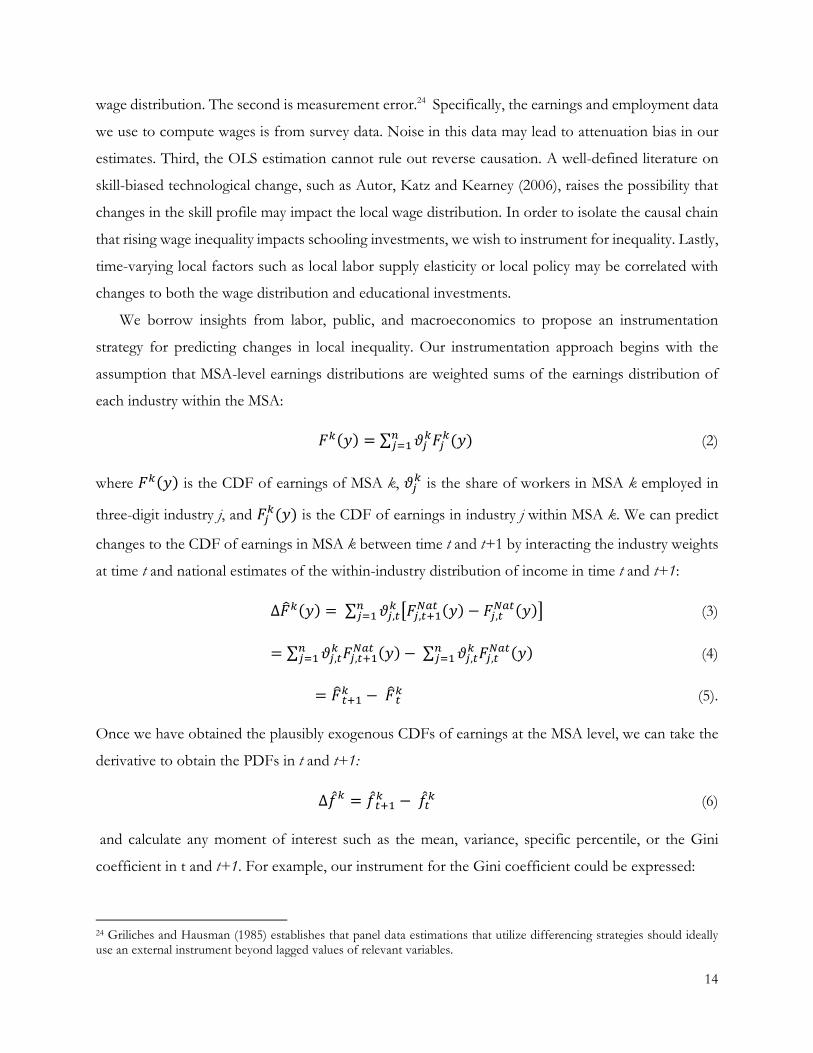
(B)*+ = ∑ -.B(.B)*+�./� (2)
where (B)*+ is the CDF of earnings of MSA k, -.B is the share of workers in MSA k employed in
three-digit industry j, and (.B)*+ is the CDF of earnings in industry j within MSA k. We can predict
changes to the CDF of earnings in MSA k between time t and t+1 by interacting the industry weights
at time t and national estimates of the within-industry distribution of income in time t and t+1:
∆(0B)*+ = ∑ -., B 2(., 3�4& )*+ − (., 4& )*+6�
./� (3)
= ∑ -., B (., 3�4& )*+ −∑ -., B (., 4& )*+�
./��./� (4)
= (0 3�B −(0 B (5).
Once we have obtained the plausibly exogenous CDFs of earnings at the MSA level, we can take the
derivative to obtain the PDFs in t and t+1:
∆78B = 78 3�B −78 B (6)
and calculate any moment of interest such as the mean, variance, specific percentile, or the Gini
coefficient in t and t+1. For example, our instrument for the Gini coefficient could be expressed:
24 Griliches and Hausman (1985) establishes that panel data estimations that utilize differencing strategies should ideally use an external instrument beyond lagged values of relevant variables.
15
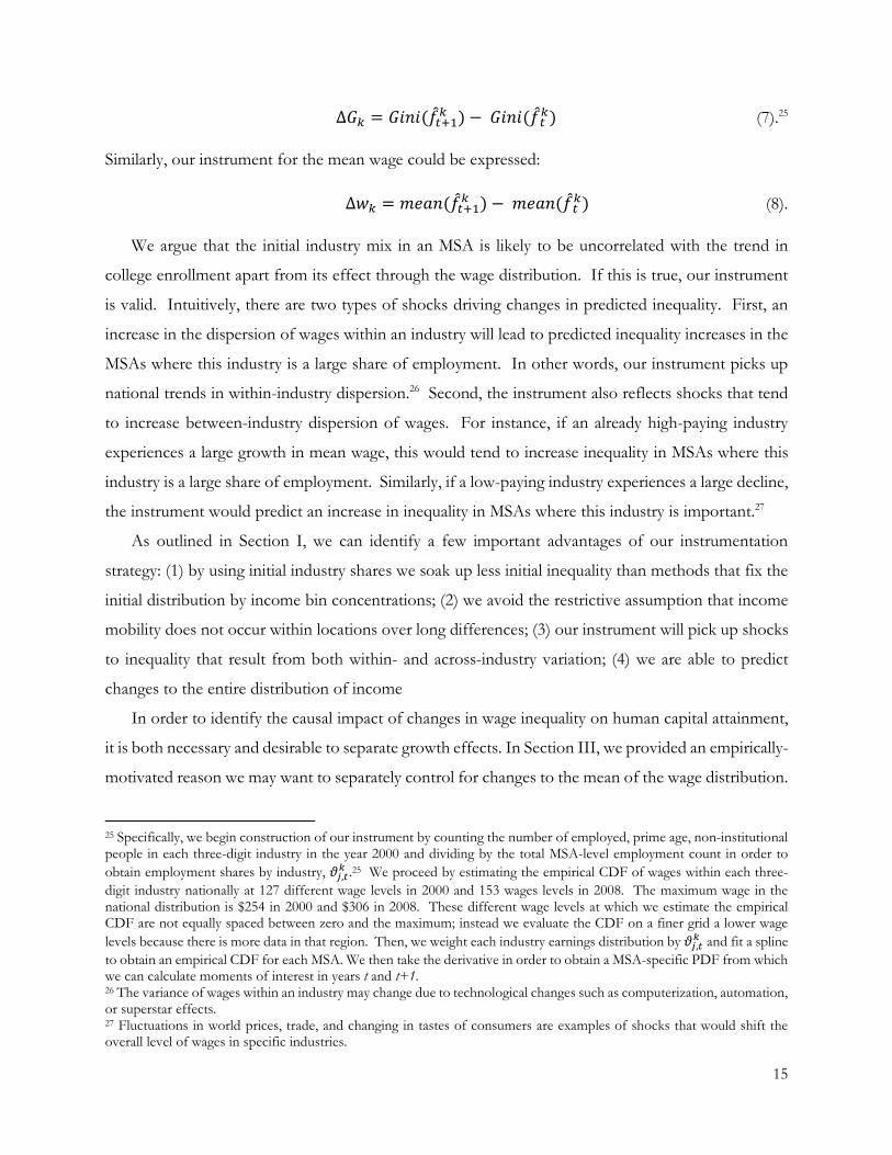
∆�B = ����)78 3�B + −����)78 B+ (7).25
Similarly, our instrument for the mean wage could be expressed:
∆9B = ��:�)78 3�B + −��:�)78 B+ (8).
We argue that the initial industry mix in an MSA is likely to be uncorrelated with the trend in
college enrollment apart from its effect through the wage distribution. If this is true, our instrument
is valid. Intuitively, there are two types of shocks driving changes in predicted inequality. First, an
increase in the dispersion of wages within an industry will lead to predicted inequality increases in the
MSAs where this industry is a large share of employment. In other words, our instrument picks up
national trends in within-industry dispersion.26 Second, the instrument also reflects shocks that tend
to increase between-industry dispersion of wages. For instance, if an already high-paying industry
experiences a large growth in mean wage, this would tend to increase inequality in MSAs where this
industry is a large share of employment. Similarly, if a low-paying industry experiences a large decline,
the instrument would predict an increase in inequality in MSAs where this industry is important.27
As outlined in Section I, we can identify a few important advantages of our instrumentation
strategy: (1) by using initial industry shares we soak up less initial inequality than methods that fix the
initial distribution by income bin concentrations; (2) we avoid the restrictive assumption that income
mobility does not occur within locations over long differences; (3) our instrument will pick up shocks
to inequality that result from both within- and across-industry variation; (4) we are able to predict
changes to the entire distribution of income
In order to identify the causal impact of changes in wage inequality on human capital attainment,
it is both necessary and desirable to separate growth effects. In Section III, we provided an empirically-
motivated reason we may want to separately control for changes to the mean of the wage distribution.
25 Specifically, we begin construction of our instrument by counting the number of employed, prime age, non-institutional people in each three-digit industry in the year 2000 and dividing by the total MSA-level employment count in order to
obtain employment shares by industry, -., B .25 We proceed by estimating the empirical CDF of wages within each three-
digit industry nationally at 127 different wage levels in 2000 and 153 wages levels in 2008. The maximum wage in the national distribution is $254 in 2000 and $306 in 2008. These different wage levels at which we estimate the empirical CDF are not equally spaced between zero and the maximum; instead we evaluate the CDF on a finer grid a lower wage
levels because there is more data in that region. Then, we weight each industry earnings distribution by -., B and fit a spline
to obtain an empirical CDF for each MSA. We then take the derivative in order to obtain a MSA-specific PDF from which we can calculate moments of interest in years t and t+1. 26 The variance of wages within an industry may change due to technological changes such as computerization, automation, or superstar effects. 27 Fluctuations in world prices, trade, and changing in tastes of consumers are examples of shocks that would shift the overall level of wages in specific industries.

16
Over the 2000s, many MSAs that experienced growth in mean wages also experienced increases in the
Gini coefficient in wages. Further, there is a theoretically-motivated reason we may wish to separate
growth effects—specifically, there may be differing theoretical predictions for the relationship
between inequality and schooling and growth and schooling. Rational agents compare the costs and
benefits of postsecondary education. An important component of educational costs is foregone
earnings.28 An empirical literature finds that increasing wages of low-skill workers, disincentivizes
postsecondary schooling.29
For these reasons, we modify our strategy by separately analyzing the effects of changes in mean
wages on enrollment rates. We could modify equation (1) to include predicted changes to the Gini
coefficient and a control for the change in mean wages:
∆���������AB = DE + D�∆�;�;<B + D=∆9:>�B + ��B + �B +�B (9).
Including actual changes in mean wages would subject our conclusions about D=, the effect of
wage growth on enrollment rates, to the same identification concerns as using actual changes in
inequality: measurement error, contamination from time-varying local unobservables such as policy,
and reverse causation. Thus, we utilize our instrumentation strategy to separately shock mean wages.
B. Identification
The main specification that we will use in testing the causal relationships between changes in
inequality and schooling and changes in growth and schooling is a Two Stage Least Squares (2SLS)
model with simultaneous first stages. We characterize the first stage for predicting changes in mean
wages:
∆9:>�B =∝E+∝� ∆9B +∝= ∆�B +��B +�B (10)
28 This is a common feature of human capital models such as Mincer (1958) and Becker (1964). 29 Charles, Hurst and Notowidigdo (2015) show strong evidence that individuals respond to increases in the opportunity cost of going to college: in the 2000s MSAs experiencing rapid growth in housing-related employment had lower enrollment in postsecondary institutions. Black, McKinnish and Sanders (2005) use coal-related booms and busts in the Appalachian States to show that an increase in the wage of low-skilled workers reduces incentives to enroll in high school. They estimate that a 10% increase in the low-skilled workers’ wage lead to a 5 to 7% decrease in high school enrollment rates. Atkin (2012) shows that growth in export manufacturing in Mexico decreased human capital investment by increasing the low-skilled wage therefore raising the opportunity cost of schooling for students at the margin.

17
where ∆9B is the distributional instrument to predict changes to mean wages, ∆�B is the distributional
instrument to predict changes in the Gini coefficient, �B is a vector of baseline controls, and �Bis a
mean-zero noise term.
We characterize the first stage for predicting changes in the Gini coefficient in wages:
∆����B =@E + @�∆9B +@=∆�B +��B +�B (11)
where ∆9B is the distributional instrument to predict changes to mean wages, ∆�B is the distributional
instrument to predict changes in the Gini coefficient, �B is a vector of baseline controls, and �Bis a
mean-zero noise term.
Thus, the second stage which is our main estimating equation is expressed:
∆���������AB = DE + D�∆�;�;<B + D=∆9:>�A B + ��B +�B (12).
where ∆9:>�A B is the predicted mean wage for MSA k from the equation (10) and ∆�;�;<B is the
predicted Gini coefficient in wages for MSA k from equation (11). The coefficient D� is the effect of
changes in local inequality on enrollment rates and D= is the effect of changes in growth on enrollment
rates.
Table 2 presents the first stage results. The top two panels present first stage results for a model
which predicts changes to the Gini coefficient in wages and mean wages. The final two panels present
first stage results for a model which predicts changes to the 90-50 difference in log wages and mean
wages. The first panel presents the point estimates for ∝�. Column 1 presents results for a reduced
model. The slope coefficient from the regression of actual changes in mean wages on predicted
changes in the mean instrument from 2000 to 2008 is 1.24 with standard error 0.25. The first stage F
statistic from the reduced model of the change in mean wages on the mean instrument is 24.12.
Column 2 presents results for a controlled model with baseline controls for log population, black share
of the population, share of the population that is non-native and does not have four-year college
attainment, and share of the population that had four-year college attainment in 1980. The slope
coefficient from the controlled regression of actual changes in mean wages on the mean instrument
from 2000 to 2008 is 1.64 with standard error 0.31. The first stage F statistic from the controlled
model of the change in mean wages on the shift-share mean instrument is 28.72. Across specifications,
the mean instrument positively predicts changes in mean wages with first stage F statistics well over
the rule of thumb of 10.

18
The second panel presents the point estimates for @�. Column 1 presents results for a reduced
model. The slope coefficient from the regression of actual changes in the Gini coefficient in wages on
the distributional instrument for the Gini coefficient from 2000 to 2008 is 1.00 with standard error
0.26. The first stage F statistic from the reduced model is 14.85. Column 2 presents results for a
controlled model with baseline controls for log population, black share of the population, share of the
population that is non-native and does not have four-year college attainment, and share of the
population that had four-year college attainment in 1980. The slope coefficient from the controlled
regression is 0.96 with standard error 0.29. The first stage F statistic from the controlled is 11.25. As
with the first stage for changes in mean wages, the instrument positively predicts changes in the Gini
coefficient in wages with first stage F statistics well over the rule of thumb of 10. We expect the
coefficient to be positive and close to 1.30
The third and fourth panels of Table 2 present first stage results for predicting changes in the 90-
50 difference in log wages and the mean wage. As with the Gini coefficient, we predict changes to the
upper tail well with the slope coefficient for the actual change in the 90-50 difference on the instrument
for the 90-50 ranging from 1.29 to 1.42 depending on specification with first stage F statistics ranging
from 14.72 to 19.70. Figure 5 visually represents the reduced form first stage for predicting changes
in the 90-50 difference—it plots the correlation between the 90-50 instrument and changes in the 90-
50 difference. The slope coefficient from this reduced form regression is 1.39 with a standard error of
0.34 and a first stage F statistic of 16.32.
As a final check on the first stages of our analysis, it is necessary to check the correlation between
the instrument that predicts changes in the wage distribution, the instrument for the inequality
measure of choice, and the instrument that predicts changes in the mean of the wage distribution. If
there was a high degree of collinearity between these instruments, and almost no residual variation in
the instrument for inequality after controlling for our growth instrument, our identification strategy
would fail. Figure 6a plots the correlation between the mean shift share instrument and the
distributional Gini coefficient instrument after we have residualized by log population in the base year.
30 Column 3 of Table 2 shows first stage results on the sample of 135 MSAs that are used in our analysis of community
college enrollments in the CPS. Consistent with the first stage results on the entire sample, coefficients for ∝�, ���&�%&'�
��&�%&'�$�! �B��� , are positive and significant with point estimates of 1.97 and 1.92 for the models including the Gini
coefficient and 90-50 instruments respectively. The first stage F statistics are over the rule of thumb of 10 with values 18.53 and 18.62 for the models including the instruments for the Gini coefficient and 90-50 respectively. The coefficient
for �#$�$C��DD$C$�� %&'�!
#$�$$�! �B��� is positive and significant with point estimate 1.83 with first stage F statistic of 15.35. The
coefficient for �EEFGE%&'�!
EEFGE$�! �B��� is positive and significant with point estimate 1.42 with first stage F statistic of 19.70.

19
Figure 6b plots the correlation between the mean shift share instrument and the distributional 90-50
difference instrument after we have residualized by log population in the base year. If all of the MSAs
were lined up on the fit line, we would conclude that our dual instrumentation strategy relies on few
locations to provide identification. In contrast, we see in both Figures 6a and 6b that many locations
lie off of the regression line. There is a negative gradient between both changes in the mean instrument
and changes in the Gini coefficient instrument and changes in the mean instrument and changes in
the 90-50 instrument. The adjusted R square for the regression of the Gini coefficient instrument on
the mean instrument is 0.03 which suggests that there is considerable variation in the predicted Gini
coefficient once we control for growth. With respect to the relationship between the instruments for
the 90-50 and the mean, we can see that they are more (inversely) related than the Gini coefficient
instrument and the mean instrument. However, the R square for the regression of the 90-50
instrument on the mean instrument is 0.07.
V. Effects of Inequality and Growth on Postsecondary Schooling
Our analysis of the causal impacts of rising wage inequality on human capital investments focuses
on first-time, full-year enrollments as the main outcome of interest. We use both administrative and
survey data in our estimations.31 Through the National Center for Education Statistics (NCES), the
US Department of Education collects enrollment information for all degree-granting, postsecondary
institutions that participate in federal financial aid programs authorized under Title IV of the Higher
Education Act of 1965. The NCES releases fall enrollment counts to the public through the IPEDS
survey. In order to construct aggregate and gender-specific enrollment counts per MSA, we use a
version of the IPEDS data set in which the MSA has been hand-coded.32 Enrollment counts are
aggregated to the MSA level. We match 192 MSAs to the sample of MSAs for which we computed
mean wage and Gini coefficients in the Census/ACS data. As the IPEDS survey is administrative data
and less prone to measurement error, our main findings focus on this data set. It should be noted that
the IPEDS survey presents aggregate enrollment counts with information tied to the institution and
not the student. This introduces a limitation in terms of controlling for relevant student characteristics
31 We focus on enrollment instead of attainment outcomes because we cannot observe degree completion in the administrative data. We are particularly interested in effects of inequality and growth on the population on the margin of community college attendance. In the survey data, it is difficult to truly measure Associate and other two-year degree completion without scooping up students in early years of bachelor-degree programs. The educational attainment outcomes constructed from survey data such as the CPS or Census and ACS would also more likely introduce contamination effects of endogenous migration. Therefore, we focus on enrollments. 32 We thank Kerwin Charles, Erik Hurst and Matthew Notowidigdo for sharing the hand-matched IPEDS data.
20
such as age, race, family structure and parental income. Importantly, the MSA identifier is tied to the
address of the institution and not the address of the student. To the extent to which students exit the
MSA that they grew up in, this could be problematic. Lau (2014) provides evidence from the Beginning
Postsecondary Survey (BPS) that this may be of less concern for community college enrollments as
the median distance from family home of a community college student is about 10 miles. In contrast,
this may be more problematic for four-year institution students as the median distance from family
home to college is about 50 miles.
In addition to the administrative data from IPEDS, we also use survey data, the Historical October
Education Supplement to the Current Population Survey (CPS), to provide robustness checks to the
main results. Our CPS sample is constructed from individual-level extracts from the IPUMS CPS
database (King et al., 2010). It is worth noting the disadvantages of the CPS; namely, we are restricted
to a smaller set of MSAs and responses may be prone to recall or other reporting error. An advantage
of the CPS lies in the ability to extract information at the student level such as age and broad residence
location.
In both the IPEDS and CPS, we evaluate effects on community college and four-year enrollments.
Community college enrollments include counts for community and technical colleges. Four-year
university enrollments include counts for public and private universities that grant bachelor degrees.
Institutions that do not receive federal financial aid through Title IV are not included in our IPEDS
data set.33 For the IPEDS analysis, we construct enrollment rates by scaling enrollment counts by the
non-institutional population age 18 to 25. In order to obtain yearly population counts, we use data
from the 1990 and 2000 Census and the 2005 to 2011 ACS. We interpolate populations for the years
1994 to 1999 and 2001 to 2004 by using a linear approximation. For the CPS analysis, enrollment rates
are calculated by combining information from questions asked about full-time enrollment status,
current year in school, and type of institution. We construct first-time, full-year enrollment counts by
counting people age 18 to 25 in first-year of community college or a four-year institution on a full-
time basis and scale by the population of non-institutional people age 18 to 25 from the CPS. For the
33 Because some for-profit schools do not receive Title IV funds, these institutions are underrepresented in IPEDS. This sector has been growing fast in recent decades. As documented in Ruch (2001), the number of for-profit postsecondary institutions grew by 112% from 1990 to 2001. To the extent to which students who attend in for-profit institutions are observably different than those who attend traditional two-year and four-year institutions, this exclusion may be important. Lau (2014) presents evidence from the Beginning Postsecondary Survey (BPS) that students who attend for-profit institutions are older, score lower on the SAT, have lower high school GPAs, are more likely to hold a GED, are less likely to receive financial support from family, and are more likely to have come from single parent, low-income homes. We should observe these students in the CPS data, however.

21
CPS, we only include MSAs with sufficient observations of non-institutional people age 18 to 25 with
non-missing educational information.
Our analysis focuses on two long differences: a difference concurrent with the shock to inequality
and a delayed long difference. For the concurrent long difference, our dependent variable is the mean
enrollment rate for years 2001 to 2008 minus the mean enrollment rate for years 1994 to 2000. We
view the years 1994 to 2000 as untreated period as they pre-date the inequality shock that we
constructed. We assume that any inequality shocks that occurred in the pre-period are orthogonal to
the constructed shock. For the delayed difference, in IPEDS, our dependent variable is the mean
enrollment rate for years 2005 to 2011 minus the mean enrollment rate for years 1994 to 2000. In the
CPS, the dependent variable for the delayed difference is the mean enrollment rate for years 2004 to
2010 minus the mean enrollment rate for years 1994 to 2000. In an alternate specification using the
IPEDS data, we difference enrollments for the year 2000 from average enrollments for the pooled
years 2006 to 2008. This strategy matches the pooling and differencing strategy used in construction
of the right hand side variables but may introduce more noise in terms of measurement of enrollment
rates.
In all of the human capital estimations, we include baseline controls for log population, black share
of the population, female employment share, share of the population that is non-native and does not
have four-year college attainment, and share of the population that had four-year college attainment
in 1980. We control for base year population, black share, female labor force participation, and low
immigrant share due to accessibility concerns. Large urban areas may have an infrastructure in place,
such as public transportation, which improves access to local campuses or may simply have more
institutions to choose from. The black share of a population may be correlated to accessibility issues
related to discrimination. The female employment share may also be related to discrimination and also
to affordable local childcare resources. Areas with large low immigrant shares may see lower
enrollments due to language-related accessibility issues. Finally, as noted in Glaeser, Resseger and
Tobio (2009), some cities have a legacy of postsecondary education which is highly correlated with
current human capital outcomes such as high school drop-out rates. Therefore, we control for
historical levels of human capital. All regressions are weighted by log population in the year 2000.
Standard errors are clustered at the state level to account for potential correlation arising from state-
level policy interventions.
Although enrollment rates in the IPEDS survey and CPS should be similar, they differ with the
CPS four-year enrollment counts outpacing those from IPEDS over the 2000s and the CPS two-year

22
enrollment counts falling below those from IPEDS for much of the 2000s.34 Figure 7 presents trends
in enrollment counts for community college and four-year institutions over the 2000s. For the 192
MSAs included in our analysis from IPEDS, the cross-MSA mean total enrollment rate in community
college for the years 1994 to 2000 was 5.20%. There is considerable variation across MSAs in baseline
enrollments. The lowest enrollment MSA for community college had an enrollment rate of 0.36%
compared to the highest enrollment MSA which had an enrollment rate of 19.32%. The cross-MSA
mean enrollment rate in four-year institutions for the years 1994 to 2000 was 6.33%. The lowest
enrollment MSA had an enrollment rate of 0.01% compared to the highest enrollment MSA which
had an enrollment rate of 26.21%. For the 135 MSAs included in our analysis from the CPS, the cross-
MSA mean total enrollment rate in community college for the years 1994 to 2000 was 3.56%. The
cross-MSA mean total enrollment rate in community college for the years 1994 to 2000 was 7.22%.
Female enrollments in four-year institutions outpaced those of men in both IPEDS and the CPS. In
the CPS, male enrollments in community colleges was higher than that of women, however, in IPEDS
women had higher enrollment rates in community colleges.35
In the following sub-sections, we discuss results of the effects of rising wage inequality and wage
growth on community college and four-year institution enrollments. Across specifications, we find
that predicted increases in the 90-50 difference and the Gini coefficient are associated with declining
enrollments. With regard to wage growth, we find that predicted increases in mean wages are
associated with declining community college enrollments. However, changes in predicted wage growth
have no effect on four-year institution enrollments. Results are robust to including controls for
baseline characteristics of the MSA.
A. Community College Estimates
We begin our analysis of the causal impacts of rising wage inequality on postsecondary schooling
investments by focusing on first-time, full-year enrollments in two-year programs such as community
college and technical schools. Table 3 presents results in IPEDS for the difference concurrent with
the shocks to wage inequality and wage growth. We present three estimation strategies in this table:
(1) Ordinary Least Squares (OLS); (2) an Instrumental Variables (IV) strategy in which we regress the
change in average enrollments directly on the instruments; (3) an Instrumental Variables strategy that
34 This is also noted in Barrow and Davis (2012) which documents community college and four-year university enrollments in both the IPEDS survey and October CPS in the wake of the Great Recession. 35 Further summary statistics for baseline enrollment information are presented in Table 1.
23
uses Two Stage Least Squares (2SLS). The top panel of the table presents results from the OLS
estimation. Columns 1 through 3 present results for changes to the upper tail of the wage distribution,
the 90-50 difference in log wages, which approximates relative skill premium. Columns 4 through 6
present results for changes to overall inequality, the Gini coefficient in wages. In the OLS model,
actual changes in upper tail inequality, the 90-50 difference, have no effect on community college
enrollments, and all effects load on growth. A 1 standard deviation increase in the mean wage is
associated with a 0.3 percentage point decrease in aggregate enrollments. With respect to overall
inequality, a 1 standard deviation increase in the Gini coefficient is associated with a 0.2 percentage
point decrease in aggregate enrollments and gender-specific enrollments. As in the OLS model with
the 90-50, a 1 standard deviation increase in the mean wage is associated with a 0.3 percentage point
decrease in aggregate enrollments.
As discussed in Section IV, there are concerns regarding the OLS results: confounding responses
to transitory shocks, measurement error, local time-varying confounders, and reverse causation. For
these reasons, we would like to instrument.36 The bottom panel of Table 3 presents 2SLS results where
changes to mean wages, the 90-50 difference, and the Gini coefficient are predicted using a shift-share
instrument constructed by interacting initial MSA-level employment shares and national within-
industry wage distributions. A 1 standard deviation predicted increase in the 90-50 difference caused
a 0.8 percentage point decline in community college enrollments from 2000 to 2008. Moving from the
10th to the 90th percentile of changes in wage inequality corresponds to a 2.05 percentage point
decrease in first-year, full-time aggregate community college enrollments. In 2000, the cross-MSA
average enrollment rate was 5.20%. If we think of changes in the 90-50 difference as approximating
changes to the skill premium, the negative coefficient provides evidence against the skill premium
hypothesis.37 Considering predicted changes in overall inequality, a 1 standard deviation predicted
increase in the Gini coefficient caused a 0.6 percentage point decline in community college enrollments
from 2000 to 2008. Moving from the 10th to the 90th percentile of changes in wage inequality
36 To the extent that local policy affected the initial industry mix and the initial industry mix is correlated with long-term trends in enrollment, our instrumentation strategy would be subject to critique. 37 The correlation between changes in the difference in log wages of those at the 90th and the 50th percentiles of the wage difference and changes in the difference in log wages of those with and without four-year college attainment is 0.39 over the 2000s. Alternatively, we estimate a 2SLS model where we predict changes in the skill premium with an instrument for the 90th percentile in log wages. The slope coefficient on the predicted change in the skill premium is -0.51 with standard error 0.29. A 1 standard deviation predicted increase in the skill premium corresponds to a 1.03 percentage point decline in community college enrollments. This seems to provide evidence against the skill premium hypothesis, locally, with respect to community college enrollments. It should be noted that the first stage is not as strong as our other models with a first stage F statistic of 5.06.

24
corresponds to a 1.54 percentage point decrease in first-year, full-time aggregate community college
enrollments. A 1 standard deviation predicted increase in mean wages caused a 0.4 percentage point
decline in community college enrollments from 2000 to 2008 although growth effects are not
significant once we instrument for either the 90-50 or the Gini coefficient.
The second panel of Table 3 presents the results for regressing directly on the instruments for
inequality and growth. A 1 standard deviation increase in the instrument for the 90-50 caused a 0.5
percentage point decline in community college enrollments. A 1 standard deviation increase in the
instrument for the Gini coefficient caused a 0.3 percentage point decline in community college
enrollments. The standardized coefficients for changes in the instruments for the 90-50 and the Gini
coefficient are smaller than the standardized coefficients from the 2SLS results.
In considering the impacts of changes to the wage distribution on human capital investment, we
may wish to consider longer term impacts. Table 4 presents results in IPEDS for the delayed
enrollment response. The dependent variable is the mean community college enrollment rate for years
2005 to 2011 minus the mean community college enrollment rate for years 1994 to 2000. Again, in
the OLS estimations, growth seems to have the strongest effects. A 1 standard deviation increase in
mean wages is associated with 0.5 and 0.4 percentage point declines in community college enrollments
in the models where we control for changes in the 90-50 and the Gini coefficient respectively. The
2SLS results for inequality are larger than the standardized effects on inequality from the shorter term
effects. A 1 standard deviation predicted increase in the 90-50 caused a 1.0 percentage point decline
in community college enrollments from 2005 to 2011. A 1 standard deviation predicted increase in
the Gini coefficient caused a 0.7 percentage point decline in community college enrollments from
2005 to 2011.
We verify the robustness of the causal impact of rising inequality on community college
enrollments established in Table 3 in the administrative data by turning to survey data. The bottom
panel of Table 5 presents 2SLS results for the effects of rising wage inequality and wage growth on
community enrollment rates as calculated in the CPS October Education Supplement. A 1 standard
deviation increase in the 90-50 caused a 0.5 percentage point decline in community college enrollments
from 2000 to 2008. A 1 standard deviation increase in the Gini coefficient caused a 0.6 percentage
point decline in community college enrollments from 2000 to 2008. Moving from the 10th to the 90th
percentile of the change in the Gini coefficient caused a 1.54 percentage point decrease in aggregate
enrollments. From 1994 to 2000, the cross-MSA average community college enrollment rate was
7.22%. Increased growth depressed community college enrollments. A 1 standard deviation increase
25
in predicted mean wages decreased community college enrollments by 0.5 and 0.3 percentage points
in models that control for predicted changes to the 90-50 and the Gini coefficient respectively.
As a falsification test on our main findings in the IPEDS data, we regress changes in first-time,
full-year enrollments from the period from 1990 to 2000 on the predicted changes in the 90-50
difference and mean wage, and the Gini coefficient and mean wage, using our shift-share
instrumentation strategy. If the changes in inequality predicted by our instruments is predictive of
changes to enrollments in the period pre-dating the shock, we may be worried that MSAs that are
moved by the instrument are serially different than those who do not receive large shocks in predicted
inequality. In the 2SLS model in which we regress changes in first-time, full-year community college
enrollments on predicted changes in the Gini coefficient, the slope coefficient is highly insignificant:
-0.23 with standard error of 2.17. The coefficient on growth is positive and also highly insignificant:
0.002 with standard error of 0.020. In the 2SLS model in which we regress changes in first-time, full-
year community college enrollments on predicted changes in the 90-50, the slope coefficient is
negative and insignificant: -0.37 with standard error of 0.38. The coefficient on growth is negative and
also highly insignificant: 0.002 with standard error of 0.018.
B. Four-Year Institution Estimates
Our analysis separately analyzes the effects of rising wage growth and inequality by postsecondary
schooling type for two important reasons. First, the tuition and time costs, entry requirements, and
benefits to a bachelor’s degree exceed those of an associate’s degree. Second, there may be a degree
of substitution across classes of degrees. As a preview of the results, we find that rising predicted wage
inequality causes modest declines in four-year enrollments. This result suggests that the decline in
community college enrollments is not resulting from substitution from community college to four-
year institutions.
Using the IPEDS data on first-time, full-year enrollments in bachelor-degree-granting institutions,
Table 6 presents results for the effects of changes in wage inequality and growth on university
enrollments. The top panel of Table 6 presents results from the OLS estimation. With respect to upper
tail inequality, a 1 standard deviation increase in the 90-50 corresponds to a 0.1 percentage point
decline in four-year college enrollments.38 A 1 standard deviation increase in the Gini coefficient is
38 Alternatively, we estimate a 2SLS model where we predict changes in the skill premium with an instrument for the 90th percentile in log wages. The slope coefficient on the predicted change in the skill premium, which is insignificant, is 0.05 with standard error 0.14. A 1 standard deviation predicted increase in the skill premium corresponds to a 0.09 percentage point increase in first-time, full-year four-year college enrollments.
26
associated with a 0.2 percentage point decrease in aggregate enrollments and gender-specific
enrollments. This result is significant and consistent with the standardized effects from the OLS
estimations on community college enrollments in Table 3. The OLS results for growth point to a
positive association between rising mean wages and four-year enrollments.
In the bottom panel of Table 6, the 2SLS model, we instrument for changes to the 90-50, Gini
coefficient, and mean wage using our shift-share instrumentation strategy. Although the slope
coefficients are insignificant, the sign is suggestive that potential students in MSAs that received
predicted inequality shocks did not substitute from community college enrollment to four-year
enrollment. Once we instrument for changes to the Gini coefficient, a 1 standard deviation change in
inequality corresponds to a 0.3 percentage point decline in four-year enrollments. A 1 standard
deviation predicted increase in the 90-50 corresponds to a 0.1 percentage point decline in four-year
enrollments. Once we instrument for changes to mean wages, the standardized coefficients from
growth attenuate.
Table 7 presents the delayed results in IPEDS for four-year institution enrollments. The
dependent variable is mean four-year enrollment rate for years 2005 to 2011 minus mean four-year
enrollment rate for years 1994 to 2000. As with the earlier period regression, the OLS effects for
predicted changes in the 90-50 are small and insignificant. With respect to overall inequality, a 1
standard deviation increase in the Gini coefficient is associated with a 0.3 percentage point decrease
in aggregate enrollments. A 1 standard deviation increase in mean wages increases four-year institution
enrollments by 0.4 percentage points. As with the IPEDS results in Table 6, once we instrument, the
point estimates for inequality and growth are not statistically significant and growth effects in the
lagged difference attenuate once we instrument. In the 2SLS model in the bottom panel of Table 7,
results for the 90-50 are highly insignificant. A 1 standard deviation predicted increase in the Gini
coefficient causes a 0.3 percentage point decrease in four-year institution enrollments.
Table 1 of the Appendix extends the analysis on four-year institution enrollments to the CPS data.
While the results from the CPS are largely insignificant, we do see negative effects of increases in
actual and predicted wage inequality on four-year enrollments. It is interesting to note that in the CPS,
the point estimates on actual and predicted increases in wage growth are positive.
In conclusion, we find that predicted increases in the 90-50 and Gini coefficient are associated
with large declines in community college enrollments. In our main analysis in the IPEDS data on
community college enrollments, we find that moving from the 10th to the 90th percentile of changes
in the 90-50 difference corresponds to a 2.05 percentage point decrease in first-year, full-time

27
aggregate community college enrollments. Further, predicted increases in mean wages are also
associated with declines in community college enrollments. This is true in the case of aggregate
enrollments, for both male and female enrollments, in the CPS data, in the later period and is robust
to the inclusion of baseline controls and to a falsification test. In the four-year institution enrollment
results, we also find evidence that predicted increases in inequality are associated with declines in first-
time, full-year enrollments in both the IPEDS survey and CPS. However, in the IPEDS survey, we
find no impacts of changes in growth on enrollments once we instrument. In the CPS, we do find
some evidence that predicted increases in mean wages are associated with increases in four-year
institution enrollments however these results are mostly not statistically significant.
The robust findings of the negative impact of increasing local wage inequality on community
college and four-year institution enrollments may suggest that a mechanism outside of the rising skill
premium may be at play.
VI. Migration
Papers utilizing regional variation are subject to concerns about selected migration. An
established literature on regional labor markets has highlighted that regional migration is a response
to employment shocks and these responses may differ by skill level.39 In this section, we address the
issue of migration by: (1) establishing that MSAs that receive large predicted inequality shocks
experience population increases among those ages 18 to 25; (2) discuss and sign the nature of the
potential bias from selected migration; and (3) show evidence that suggests our findings are not
quantitatively altered by the migration responses in the sample.
To begin, we are interested in migration of young, potential students in response to changes in
inequality and growth. Table 2 of the Appendix regresses changes in population of non-institutional
people age 18 to 25 on changes in the 90-50, the Gini coefficient and mean wages. Columns 1 and 2
examine these effects in a model where we shock upper tail inequality, the 90-50 difference in wages,
controlling for changes to mean wages. Column 1 examines effects for the whole age 18 to 25
population which would include migration from abroad, other states, and other locations within the
state. Column 2 examines changes in the population of people age 18 to 25 who reside in their state
of birth; changes in this variable would represent intrastate migration. In the OLS results, there are no
39 Blanchard and Katz (1992) document regional migration responses to rising unemployment. In Glaeser and Gyourko (2005), college workers exit cities with negative labor demand shocks. In Topel (1986), and Bound and Holzer (2000), non-college workers are less mobile than college workers. In Notowidigdo (2011), the progressive nature of transfer program eligibility formulas induces low skill workers to remain in areas with negative demand shocks.
28
significant effects of changes in inequality on population. In the instrumented model in the center
panel of Table 2 of the Appendix, we find predicted increases in inequality cause increases in
population. A 1 standard deviation increase in the instrument for the 90-50 increases the population
of those age 18 to 25 by 0.31 of 1 standard deviation. A 1 standard deviation increase in the
distributional instrument for the 90-50 increases the native-state population of those age 18 to 25 by
0.23 of 1 standard deviation. We find that wage growth also has a positive effect, yet insignificant, on
population growth. A 1 standard deviation increase in the mean wage instrument increases the
population of those age 18 to 25 by 0.04 of 1 standard deviation. A 1 standard deviation increase in
the mean wage instrument increases the native-state population of those age 18 to 25 by 0.10 of 1
standard deviation. In the bottom panel, we present the 2SLS estimates. A 1 standard deviation
predicted increase in the 90-50 corresponds to 0.47 of a 1 standard deviation increase in the total
population age 18 to 25 and a 0.34 of a 1 standard deviation increase in the native population age 18
to 25. With respect to mean growth, a 1 standard deviation predicted increase in mean wages causes a
0.09 and 0.13 of a 1 standard deviation increase in the total and native populations respectively. The
growth effects on the native population are significant.
Columns 3 and 4 examine these effects in a model where we shock overall inequality, the Gini
coefficient in wages, controlling for changes to mean wages. Column 3 examines effects for the whole
population age 18 to 25, and Column 4 examines changes in the population of people age 18 to 25
who currently reside in their state of birth. Consistent with the 90-50 results, the OLS results are not
significant for inequality. The 2SLS results for the Gini coefficient, presented in the bottom panel of
Table 2 of the Appendix, also yield large population increases. A 1 standard deviation predicted
increase in the Gini coefficient corresponds to 0.47 of a 1 standard deviation increase in the total
population age 18 to 25 and a 0.33 of a 1 standard deviation increase in the native population age 18
to 25. With respect to growth, a 1 standard deviation predicted increase in mean wages causes a 0.08
and 0.12 of a 1 standard deviation increase in the total and native populations respectively; however,
growth effects are not significant.
We have established that MSAs that experienced large predicted increases in both upper tail and
overall inequality experienced population booms both in the form of overall migration and intrastate
migration. As we are focused on human capital outcomes, migration may be particularly concerning
if migrants look different than nonmigrants on the basis of human capital attainment. Our outcome
variable is first-time, full-year enrollees at community colleges and four-year institutions. If young
migrants have already attained postsecondary education, they will be less likely to be first-time

29
enrollees. An increase in this type of migration would cause enrollment rates to decline as the
denominator increases. If high income parents migrate into MSAs with predicted increases in wage
inequality and their children are more likely to enroll in postsecondary schooling, we may see an increase
in enrollments due to the change in composition. Likewise, if young migrants have a latent taste for
human capital, even if they migrate without higher levels of human capital attainment, they may be
more likely to seek postsecondary schooling. This would result in increases in enrollment rates in the
presence of this form of selected migration. In our main analyses, we estimated negative effects of
predicted changes in inequality on community college and four-year enrollments. Thus, if these
mechanisms were at work, our main results would be even more negative in the absence of migration.
In the presence of selected migration, enrollment rates may decline even in the presence of
increasing enrollment counts if increasing inequality bids migrants into a MSA. If we only focused on
changing enrollment rates, this type of migration may lead us to falsely reject the skill premium
hypothesis due to population effects churning through the denominator. For this reason, it is
imperative to consider separately the numerator: enrollment counts. We estimate a 2SLS model using
the difference in enrollment counts instead of enrollment rates. For community college enrollments,
the slope coefficient on the predicted change in the 90-50 is -45858.56 with standard error 15470.56.
The slope coefficient on the predicted change in the Gini coefficient is also negative: -219205.8 with
standard error 105738.3. With respect to four year enrollment counts, the slope estimates in counts
are not significant. The slope coefficient on the predicted change in the 90-50 is 433.13 with standard
error 12891.54. The slope coefficient on the predicted change in the Gini coefficient is negative which
is consistent with the results in rates, but is not significant: -32053.33 with standard error 40461.24.
We find that absolute enrollment levels are declining even as the population of those age 18 to 25 is
increasing. Thus, our main findings are truly the result of declining enrollment activity not due to local
population changes.
Although overall migration of people age 18 to 25 is increasing in MSAs with large predicted
shocks in inequality, the causal effect of changes in inequality on community college enrollments is
still present absent population changes. Now, we take a deeper look into the type of people who are
migrating. As discussed in the previous section, the IPEDS survey does not provide information about
the characteristics of students. Thus, we cannot separate migrants from nonmigrants in the IPEDS
data. However, the March Historical CPS does provide information on the migration status of
30
individuals.40 Using information from a question of recent migration status, we are able to identify
migrants in the sample.41 Following the pooling strategy we used in construction of the CPS education
variables, we compute several summary statistics of interest for the 135 MSAs used in the CPS
aggregate analyses over the periods 1994 to 2000 and 2001 to 2008. Figure 8 compares demographic
characteristics of young migrant and nonmigrant populations in MSAs within and across periods
depending on whether the MSA has an above- or below-median predicted change in the Gini
coefficient. In Figure 8, we can clearly see that migrants are different than nonmigrants on at least
two dimensions: they are more likely to be white and more likely to have four-year college attainment.
However, across MSAs that receive large predicted increases in inequality and those that do not, these
patterns are stable.
In conclusion, we find that MSAs that receive large predicted increases in inequality have
population increases. However, once we remove population effects by using enrollment counts
instead of enrollment rates as our outcome variable, our main results are still present. In the CPS, we
find migrants are slightly more likely to be white and more educated than young nonmigrants.
However, the differences between migrant and nonmigrant populations are similar across large
predicted inequality and small predicted inequality MSAs and are stable over time. Thus, we do not
think that education results from the CPS are a product of selected migration.
VII. Effects of Inequality and Growth on Residential Segregation by Income
This section explores the impact of rising local wage inequality on an important feature of local
community—the income composition of neighborhoods. Income segregation refers to the spatial
distribution of income across neighborhoods. Income segregation is therefore a different concept than
wage inequality though the latter is a necessary condition: In MSAs in which most of the community’s
income is held by a small group, the rich can select to disperse throughout the MSA’s neighborhoods
or reside in a selected few neighborhoods. A segregated MSA would be one in which richer individuals
tend to live in the same neighborhoods while poor families would live close to each other.
There are two channels through which income segregation potentially matters to skill acquisition
and human capital investment: (1) fiscal externalities; and (2) “sociological or psychological effects”42.
40 In our analysis on enrollments, we use the October CPS which does not have migration variables. Thus, in this exercise we use the March CPS which does have migration variables and restrict to the same MSAs used in the October CPS to gain insight into the characteristics of migrants and nonmigrants in the MSAs used in our analysis. 41 We use the variable migrate1 in IPUMS CPS and identify migrants as people who did not live in the same house or the same county the year before. 42 For a survey of the literature on neighborhood effects see Durlauf (2004).

31
To the extent that individuals with different income sort across governments such as school districts
and municipalities, tax revenue and therefore the amount of public goods consumed by individuals
will differ and be correlated with individual income. Generally, close proximity to rich neighbors
improves local amenities such as more and better quality parks, libraries and even schools.43 In
addition to these fiscal externalities, neighborhoods matter as networks. Neighborhoods are the first
level of community outside the boundaries of family life. As such, they serve as classrooms for one’s
earliest knowledge of the labor market and serves as an entry point into civic, political and educational
networks. Therefore, these small communities may play an important role in the formation and
accumulation of both social and human capital.
A large literature on human capital acquisition has shown the recursive nature of human capital:
current level of human capital is an important input in the production of future human capital.44 As a
result, the returns to secondary education depend heavily on the quality of an individual’s past
education which in turn may have been affected by the composition of her neighborhood. Also,
returns might be lower for individuals in poorer neighborhoods if networks and personal connections
are important in order to find a job and realize the monetary gains from higher education. Finally,
perceived returns may also be lower (or uncertain) to an individual who is not surrounded by many
educated neighbors. For these reasons, income segregation may decrease enrollment in postsecondary
education in homogenously poor neighborhoods. If individuals at the margin of college enrollment
decision are concentrated in the lower end of the income distribution, income segregation would
decrease aggregate enrollment. Durlauf (1996) and Benabou (1996) develop theoretical models in
which the productivity of investment in human capital depends on neighborhood composition. In
both models, segregation causes lower social mobility and potentially inefficient aggregate output.
Between 1980 and 2008, the cross-MSA mean difference between the 10th and the 90th percentile
of mean Census tract45 income has nearly doubled from $34,592 to $68,237 (expressed in the real
value of a dollar in 2000). Of that increase, 13% can be attributed to a change in the sorting of
households46. The change in sorting appears to have the largest incidence in poorer neighborhoods.
43 Though school funding is increasingly centralized at the state-level to limit differences in school expenditures per capita across school districts. 44 Cunha and Heckman (2007); Heckman and Mosso (2014). 45 In our empirical analysis and following much of the literature on segregation, we use Census tracts as our definition of neighborhoods. 46 Mean income in each Census tract is estimated using NHGIS’ household income data at the tract level. These data only indicates the number of households in different relatively narrow “income bins”. We assume that the tract-distribution of income within each bin perfectly mirrors the MSA distribution within that bin. The fraction of the change attributable to sorting is calculated in the following way. First, we estimate a counterfactual mean income for each tract in 2008 by

32
Around 27% of the $11,012 increase in the average difference between the 10th and the 50th
percentile of mean Census tract income can be attributed to the change in sorting of households.
These large changes in relative mean neighborhood income suggest that fiscal externalities are
potentially important.
How we define income segregation is of critical importance when discussing the relationship
between segregation and inequality. For example, if income segregation is defined as the variance of
mean neighborhood income, it is mechanically related to income inequality. Consider a city with some
positive degree of sorting across neighborhoods. If income inequality increases in that city, even
holding everyone’s location and rank in the income distribution constant, mean income in the richer
neighborhoods will increase relative to mean income in the poorer neighborhoods. In a world with
non-zero degree of income segregation, increases in income inequality have direct consequences in
terms of fiscal externalities. There is another mechanism through which increases in income inequality
translate into increased differences in mean income between poor and rich neighborhoods: sorting.
To conceptualize this mechanism, let us consider a measure of income segregation that is not
mechanically related to inequality: the Rank Order Theory Index (henceforth denoted by H).47 H is a
measure of evenness of the spatial distribution of individuals with respect to income. We could
conceptualize this measure as a variant of a Herfindahl index.48 It ranks all households in the MSA
according to their income. It then compares the distribution of “ranks” in the MSA income
distribution within each neighborhood.
Specifically, we construct this measure by following Reardon and Firebaugh (2002) and Reardon
(2011). First, we estimate H(p) at every percentile p corresponding to the endpoints of the available
income bins in each MSA. H(p) is a Theil index measuring to what extent the proportion of individuals
below percentile p in each neighborhood differs from p:
H)I+ = 1 − ∑ K�KL∗�L)K+K�KNOP∗�)K+. (I)
where j indexes Census tracts and
holding the 1980 income percentile composition of each tract constant but imputing the 2008 income corresponding to each percentile in the MSA. Second, we compute the counterfactual 90-10 difference in mean neighborhood income. Third, the fraction of the change attributable to sorting is 1-(counterfactual 90-10 difference)/(actual 90-10 difference). 47 The Rank Order Theory index is developed in Reardon and Firebaugh (2002) and Reardon (2011). It is also used in Reardon and Bischoff (2011, 2013) and in Chetty et al. (2014). 48 Herfindahl (1950)
33
�)I+ = I ∗ ��>= Q�KR + )1 − I+ ∗ ��>= Q �
�FKR (II)
Both in 2000 and 2008, 16 income bins are reported. In each MSA, H(p) is evaluated at 16 different
percentiles corresponding to the endpoints of each bin.49 In theory, the Rank Theory Index is
computed as follows:
H = 2��>=)2+ T �)I+H)I+UIK (III)
As H(p) can only be measured at 16 different percentiles, we interpolate. We fit a 4th order
polynomial using OLS to approximate H(p). Reardon (2011) shows that the Rank Theory Index is
approximately equal to a weighted sum of the coefficients of this regression.
If the distribution within each neighborhood perfectly mirrors the overall distribution in the MSA
(which is a uniform distribution), H takes value zero denoting perfect integration. If all of the variation
in ranks is across neighborhoods, H takes value one, denoting perfect segregation. Because this
measure relies only on individuals’ rank in the income distribution it is insensitive to changes that leave
everyone’s rank and neighborhood constant. Increased dispersion in the distribution of household
income will leave H unchanged as long as households’ location and rank does not change.
Data to measure segregation come from the US Census 2000 summary tape files 3A and ACS
pooled sample 2005-2009.50 For simplicity, we will refer to the 2005-2009 pooled data as the 2008
data. The summary tape files report the number of households in different income bins within each
Census tract. Income segregation is regressed on the Gini coefficient and the log difference between
the 90th and 50th percentile of the pre-tax wage distribution.
The correlation between income inequality and segregation is documented in a small literature on
income segregation and inequality.51 While we use the same measure of segregation as Reardon and
Bischoff (2011) and exploit regional variation as in Watson (2009), we improve on the existing
literature by instrumenting for income inequality. Further, we are able to disentangle growth effects
through the simultaneous use of an instrument for growth and inequality.52
49 The endpoints correspond to different percentiles in different MSAs. 50 Data are obtained through the National Historical Geographic Information System (NHGIS). 51 Mayer (2001); Watson (2009); Reardon and Bischoff (2011) 52 Watson (2009) uses a manufacturing Bartik instrument to exogenously shock income inequality. Her specification does not allow her to separate the effects of inequality from growth because the manufacturing Bartik is positively correlated with inequality but also negatively correlated with growth. She finds standardized effects as high as 0.9.
34
The results that follow indicate that the sociological environment in which poor children grow up
may change as a result of wage inequality. Specifically, we show that increases in the Gini coefficient
lead to relatively large increases in H. Moving from the 10th to the 90th percentile of the predicted
increase in the Gini coefficient in wages is associated with 0.51 of a 1 standard deviation increase in
H. Moving from the 10th to the 90th percentile of the predicted increase in the 90-50 log difference
causes a 0.67 of a 1 standard deviation increase in H. Wage inequality increases sorting of households
along income rank.
This result raises the question of the theoretical underpinnings for a causal empirical link between
inequality and segregation. The model in Durlauf (1996) exhibits theoretical support for this feature.
Because the productivity of human capital investment depends on the income distribution in the
neighborhood, the incentives to segregate increase with differences in income between rich and poor.
In the model, the mechanism through which rich segregate from the poor is the imposition of zoning
restrictions. It provides a comprehensive model tying together the location decision of families and
the consequences of neighborhood composition on families’ outcomes as well as a theoretical
motivation of why increases in income inequality might lead to increases in income segregation. In
Tiebout (1956), rich and poor individuals have different preferences over public goods; they perfectly
segregate in equilibrium because they choose to locate in neighborhoods with a different level of
public goods. Epple and Platt (1998) introduce random noise in individuals’ preferences so that
willingness to pay for public good is not perfectly correlated with income: their equilibrium exhibits
partial segregation. With an increase in income inequality, income becomes a more important
predictor of preferences over public goods relative to the random noise component of preferences.
As a result, willingness to pay for public good correlates more strongly with income and it becomes
less likely that a poor family be willing to overbid a rich family to locate in the neighborhood with
better composition: income segregation increases with inequality. In Tiebout (1956) and Epple and
Platt (1998), individuals care about the amount of public good provided in the neighborhood. More
generally, individuals may have preferences directly over their neighbors’ income or over
characteristics correlated with income as in Guerrieri, Hartley and Hurst (2013). As long as neighbors’
income is a normal good, segregation will occur.
Our estimation strategy closely matches the pooling and differencing strategy used in construction
of the right hand side variables. We difference segregation (H) in 2000 from segregation for the pooled
years 2005 to 2009. In all of the segregation estimations, we include baseline controls for log
population, black share of the population, share of the population that is non-native and does not

35
have four-year college attainment, and share of the population that had four-year college attainment
in 1980. All regressions are weighted by log population in the year 2000. Standard errors are clustered
at the state level to account for potential correlation arising from state-level policy interventions.
Table 8 shows the effects of changes in inequality and growth on residential segregation. The top
panel presents the OLS results. The OLS results reveal a strong and statistically significant association
between the Gini coefficient and income segregation. The log difference between the 90th and 50th
percentile of the wage distribution is also positively correlated with residential segregation though this
relationship is not statistically significant.
As with the human capital models, we may be concerned about drawing causal inference from the
OLS results. Neighborhood selection has potentially long-term impacts and residential ownership is
sticky. We want to assess the impact of structural changes; thus, we would like to instrument and avoid
idiosyncratic local shocks that may be picked up with our differencing strategy. As with the human
capital estimations, the OLS strategy cannot rule out reverse causation. In order to isolate the causal
chain that rising wage inequality impacts residential sorting, we wish to instrument for inequality.
Thirdly, time-varying local factors such as local labor supply elasticity or local policy may be correlated
with changes to both the wage distribution and income segregation. For these three reasons, we would
also like to instrument.
The middle panel of Table 8 shows income segregation regressed directly on the instruments. The
standardized effect on the instrument for the Gini coefficient is large, positive and statistically
significant. A 1 standard deviation increase in the instrument for the Gini coefficient in wages is
associated with 0.16 of a 1 standard deviation increase in H. A 1 standard deviation increase in the
instrument for the 90-50 log difference causes 0.16 of a standard deviation increase in the Rank Order
Theory Index.
The coefficient on growth is negative but not statistically significant in all specifications. Places
with increasing wages seem to have experienced a decrease in income segregation. A potential
explanation is that individuals care about some of their neighbors’ characteristics that are correlated
with income but these preferences may exhibit strong concavity. As a result, as all boats are lifted up,
the income-rank composition of one’s neighbor may matter less and less and decrease incentives to
segregate.
The bottom panel of Table 8 reports coefficients of a 2SLS regression of changes in income
segregation on inequality and growth using the instruments described above. Coefficients on
inequality are positive and statistically significant. A 1 standard deviation increase in the Gini

36
coefficient causes 0.19 of a 1 standard deviation increase in segregation. The standardized coefficient
on the 90-50 log difference is larger in magnitude and equal to 0.26. Coefficients on growth are
negative but not statistically significant.
Table 8 also reports the results from regressing income segregation on inequality and growth in a
smaller sample of MSAs: those for which we have enough observations to get reliable measures of
enrollment in the CPS. Our results are robust to applying this sample restriction.
VIII. Conclusion
In this paper, we introduce a novel instrument for MSA-level changes in wage inequality. This
allows us to uncover an important and surprising fact: rising local wage inequality depresses aggregate
first-year enrollment rates in postsecondary education. In addition, we provide evidence that rising
wage inequality causes increased residential sorting on an income basis. Our model predicts first-year
community college enrollments will decline by 2.6 and 2.1 percentage points over the 2000s in
response to changes in the 90-50 and Gini coefficient respectively.53 Our model predicts first-year
four-year institution enrollments will decline by 0.17 and 0.93 percentage points over the 2000s in
response to changes in the 90-50 and Gini coefficient respectively.54
We do not find significant evidence for a strong effect of growth on postsecondary schooling.
Simple correlations show that growth is positively correlated with enrollment in four year universities.
After instrumenting, we find that the effect of overall wage growth is close to zero. If anything, places
with rising overall wages seem to have experienced a decrease in community college enrollment.
The coefficient on the enrollment results suggest that the skill premium hypothesis is not at work
in response to increases in local wage inequality. One theory that suggests a negative relationship
between inequality and investment in human capital is related to neighborhood effects. Specifically,
increasing inequality may cause families to increasingly sort on an income basis. That is, rich families
outbid poor families for rich neighbors. As entire MSAs become more unequal, the residents also
become more segregated from each other. To the extent to which neighborhood composition is
influential to human capital accumulation, this may have effects on postsecondary enrollments.
Through our analysis in Section VII, we established that there is, in fact, a causal relationship between
rising inequality and increasing income segregation. We find that increasing inequality both at the
53 We calculate the model prediction by multiplying the regression coefficient from the bottom panel of Column (1) of Table 3 by the cross-MSA actual change in the Gini coefficient in wages over the 2000s. 54 We calculate the model prediction by multiplying the regression coefficient from the bottom panel of Column (1) of Table 6 by the cross-MSA actual change in the Gini coefficient in wages over the 2000s.

37
upper tail, the 90-50 difference, and over the entire wage distribution, the Gini coefficient, cause
increased residential sorting on an income basis. A 1 standard deviation predicted increase in the Gini
coefficient causes 0.20 of a 1 standard deviation increase in segregation. Similarly, at the upper tail a 1
standard deviation increase in the 90-50 difference causes 0.26 of a 1 standard deviation increase in
segregation.
This mechanism is consistent with two concerns in the public discussion: (1) inequality has an
adverse effect on growth; and (2) inequality reduces intergenerational mobility. Though this paper did
not attempt to provide direct evidence of the effect of inequality on growth and intergenerational
mobility, our findings provide indirect support for these concerns. To the extent that these effects
are mediated through neighborhood externalities, there is no guarantee that the overall amount and
distribution of human capital investment within the population is efficient. As noted in work such as
Fault Lines by Raghuram Rajan (2010), the growth in educational attainment has stalled, at least in the
1980s and 1990s, despite the presumed constant increase in relative demand for skills. Our results
speak to this apparent puzzle: as the relative demand for skilled-workers increases, the skill premium
rises and translates into higher local inequality. Individuals at the margin should respond to the
increasing skill premium by investing more in their human capital. However, this effect may be muted
if marginal individuals simultaneously became less prepared to attend college due to spillovers from
local inequality.
The efficiency of human capital investments as well as intergenerational mobility are first-order
issues; this is reflected by the space these topics currently occupy in the public forum. Our future
research agenda includes securing individual finely geocoded panel data, such as the NLSY, in order
to separately analyze the direct effect of individual and parental income from the direct and indirect
effects of a changing wage distribution on an individual’s probability of postsecondary schooling. In
addition, directly observing the response at the individual level of pre-college inputs into the
production of human capital to shocks to local inequality would help separate the mechanisms.
Another interesting direction of research could be to relate our results to measures of educational
attainment as opposed to enrollment. In order to address real effects of inequality on attainment, we
would like to have data with more detailed migration information such as IRS tax data in order to
satisfactorily confront issues related to selective migration. As a final word, although the results for
income segregation are suggestive of a mechanism for our main result, we plan to explore other
potential mechanisms, particularly those related to political economy responses to wage inequality. We

38
hope that our findings will stimulate more research into the causal effects of rising inequality on human
capital investments.

39
References Acemoglu, Daron. "Changes in Unemployment and Wage Inequality: An Alternative Theory and Some Evidence." American Economic Review 89.5 (1999): 1259-1278. Aguiar, Mark, and Mark Bils. 2015. "Has Consumption Inequality Mirrored Income Inequality?" American Economic Review, 105(9): 2725-56. Aizer, Anna. "The gender wage gap and domestic violence." American Economic Review 100.4 (2010):
1847.
Alesina, Alberto, and Dani Rodrik. "Distributive Politics and Economic Growth." The Quarterly Journal
of Economics 109.2 (1994): 465-490.
Atkin, David. “Endogenous skill acquisition and export manufacturing in Mexico”. No. w18266. National Bureau of Economic Research, 2012. Attanasio, Orazio, Erik Hurst, and Luigi Pistaferri. “The evolution of income, consumption, and leisure inequality in the US, 1980-2010.” No. w17982. National Bureau of Economic Research, 2012. Autor, David, H., and David Dorn. "The Growth of Low-skill Service Jobs and the Polarization of the US Labor Market." The American Economic Review 103.5 (2013): 1553-1597. Autor, David, H., Lawrence F. Katz, and Melissa S. Kearney. "The Polarization of the US Labor Market." The American Economic Review 96.2 (2006): 189-194. Autor, D. H., Katz, L. H., & Kearney, M. S.. “Trends in US Wage Inequality: Revising the
Revisionists”. The Review of Economics and Statistics (2008), 90(2), 300-323.
Autor, David H., Frank Levy and Richard J. Murnane. "The Skill Content of Recent Technological Change: An Empirical Exploration." The Quarterly Journal of Economics 118.4 (2003): 1279-1333.
Barrow, Lisa, and Jonathan Davis. "The upside of down: Postsecondary enrollment in the Great Recession." Economic Perspectives 36.4 (2012). Bartik, Timothy J. "Who Benefits from State and Local Economic Development Policies?" Books from Upjohn Press (1991). Becker, Gary (1964). Human Capital: A Theoretical and Empirical Analysis with Special Reference to Education.
New York: Columbia University Press.
Becker, Gary S., and Nigel Tomes. "An equilibrium theory of the distribution of income and
intergenerational mobility." The Journal of Political Economy (1979): 1153-1189.
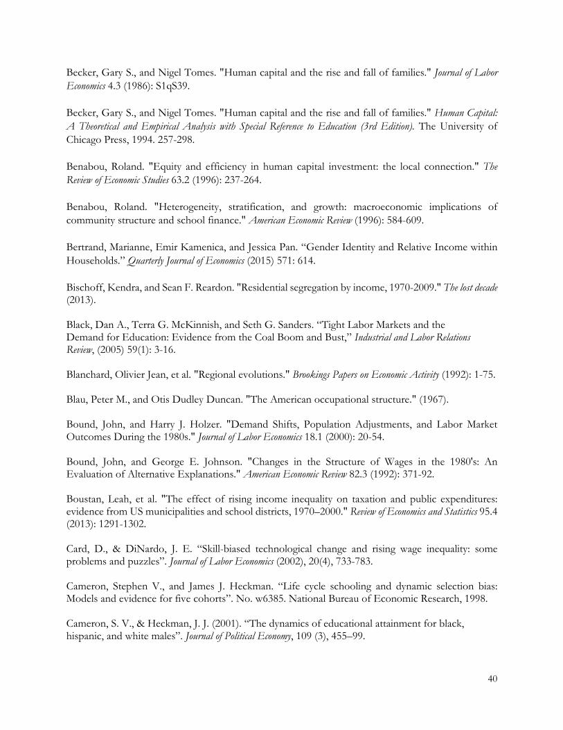
40
Becker, Gary S., and Nigel Tomes. "Human capital and the rise and fall of families." Journal of Labor
Economics 4.3 (1986): S1qS39.
Becker, Gary S., and Nigel Tomes. "Human capital and the rise and fall of families." Human Capital:
A Theoretical and Empirical Analysis with Special Reference to Education (3rd Edition). The University of
Chicago Press, 1994. 257-298.
Benabou, Roland. "Equity and efficiency in human capital investment: the local connection." The
Review of Economic Studies 63.2 (1996): 237-264.
Benabou, Roland. "Heterogeneity, stratification, and growth: macroeconomic implications of
community structure and school finance." American Economic Review (1996): 584-609.
Bertrand, Marianne, Emir Kamenica, and Jessica Pan. “Gender Identity and Relative Income within
Households.” Quarterly Journal of Economics (2015) 571: 614.
Bischoff, Kendra, and Sean F. Reardon. "Residential segregation by income, 1970-2009." The lost decade (2013). Black, Dan A., Terra G. McKinnish, and Seth G. Sanders. “Tight Labor Markets and the Demand for Education: Evidence from the Coal Boom and Bust,” Industrial and Labor Relations Review, (2005) 59(1): 3-16. Blanchard, Olivier Jean, et al. "Regional evolutions." Brookings Papers on Economic Activity (1992): 1-75. Blau, Peter M., and Otis Dudley Duncan. "The American occupational structure." (1967). Bound, John, and Harry J. Holzer. "Demand Shifts, Population Adjustments, and Labor Market Outcomes During the 1980s." Journal of Labor Economics 18.1 (2000): 20-54. Bound, John, and George E. Johnson. "Changes in the Structure of Wages in the 1980's: An Evaluation of Alternative Explanations." American Economic Review 82.3 (1992): 371-92. Boustan, Leah, et al. "The effect of rising income inequality on taxation and public expenditures: evidence from US municipalities and school districts, 1970–2000." Review of Economics and Statistics 95.4 (2013): 1291-1302. Card, D., & DiNardo, J. E. “Skill-biased technological change and rising wage inequality: some problems and puzzles”. Journal of Labor Economics (2002), 20(4), 733-783. Cameron, Stephen V., and James J. Heckman. “Life cycle schooling and dynamic selection bias: Models and evidence for five cohorts”. No. w6385. National Bureau of Economic Research, 1998. Cameron, S. V., & Heckman, J. J. (2001). “The dynamics of educational attainment for black, hispanic, and white males”. Journal of Political Economy, 109 (3), 455–99.

41
Cameron, S. V., & Taber, C. (2004). “Estimation of educational borrowing constraints using returns to schooling”. Journal of Political Economy, 112 (1), 132–182. Card, David, Thomas Lemieux, and W. Craig Riddell. "Unions and wage inequality." Journal of Labor Research 25.4 (2004): 519-559. Carneiro, P., & Heckman, J. J. (2002). “The evidence on credit constraints in post-secondary
schooling”. Economic Journal, 112 (482), 705–734.
Caucutt, Elizabeth M., Lance Lochner, and Youngmin Park. “Correlation, Consumption, Confusion, or Constraints: Why do Poor Children Perform so Poorly?”. No. w21023. National Bureau of Economic Research, 2015. Charles, Kerwin Kofi, Erik Hurst, and Matthew J. Notowidigdo. “Manufacturing Decline, Housing Booms, and Non-Employment”. No. w18949. National Bureau of Economic Research, 2013. Charles, Kerwin K., Erik Hurst, and Matthew J. Notowidigdo. "Housing Booms, Labor Market
Outcomes, and Educational Attainment." Manuscript, University of Chicago (2015).
Chetty, Raj, Nathaniel Hendren, and Lawrence F. Katz. “The Effects of Exposure to Better
Neighborhoods on Children: New Evidence from the Moving to Opportunity Experiment.” No.
w21156. National Bureau of Economic Research, 2015.
Chetty, Raj, et al. “Where is the land of opportunity? The geography of intergenerational mobility in
the United States”. No. w19843. National Bureau of Economic Research, 2014.
Chetty, Raj, et al. “Is the United States still a land of opportunity? Recent trends in intergenerational
mobility”. No. w19844. National Bureau of Economic Research, 2014.
Chetty, Raj, Nathaniel Hendren, and Lawrence F. Katz. “The Effects of Exposure to Better Neighborhoods on Children: New Evidence from the Moving to Opportunity Experiment”. No. w21156. National Bureau of Economic Research, 2015. Cochrane, John. “Why and how we care about inequality.” Web blog post. The Grumpy Economist. September 29, 2014. Cunha, F., & Heckman, J. J. “The technology of skill formation”. American Economic Review (2007), 97 (2), 31–47. Dahl, Gordon B., and Lance Lochner. "The impact of family income on child achievement: Evidence from the earned income tax credit." American Economic Review 102.5 (2012): 1927-1956. Durlauf, S. “A Theory of Persistent Income Inequality”. Journal of Economic Growth (1996), 1, 75-93.
Durlauf, Steven N. "Neighborhood effects." Handbook of regional and urban economics 4 (2004): 2173-
2242.
42
Epple, Dennis and Glenn J. Platt, “Equilibrium and Local Redistribution in an Urban Economy When Households Differ in Both Preferences and Incomes,” Journal of Urban Economics (1998), 43, 23–51. Fisher, Jonathan D., David S. Johnson, and Timothy M. Smeeding. "Measuring the trends in inequality of individuals and families: Income and consumption." The American Economic Review 103.3 (2013): 184-188. Glaeser, Edward L., and Joseph Gyourko. "Urban Decline and Durable Housing." Journal of Political Economy (2005), 113.2. Glaeser, Edward L., Matt Resseger, and Kristina Tobio. "Inequality in cities*." Journal of Regional Science
49.4 (2009): 617-646.
Goldin, Claudia and Lawrence Katz (2008). The Race Between Education and Technology, Bekknap Press.
Goos, Maarten, and Alan Manning. "Lousy and lovely jobs: The Rising Polarization of Work in Britain." The Review of Economics and Statistics 89.1 (2007): 118-133. Goos, Maarten, Alan Manning, and Anna Salomons. "Job Polarization in Europe." The American Economic Review (2009): 58-63. Griliches, Zvi, and Jerry A. Hausman. "Errors in Variables in Panel Data." Journal of Econometrics 31.1 (1986): 93-118. Guerrieri, Veronica, Daniel Hartley, and Erik Hurst. "Endogenous gentrification and housing price dynamics." Journal of Public Economics 100 (2013): 45-60.
Guryan, Jon, Erik Hurst, and Melissa Kearney. "Parental Education and Parental Time Use." Journal
of Economic Perspectives (2008): 22.
Heckman, James J., Humphries, John Eric, Veramendi, Greg and Urzua, Sergio S., “Education, Health and Wages”, No. W19971. National Bureau of Economic Research. 2014. Heckman, James J., and Stefano Mosso. “The economics of human development and social mobility”. No. w19925. National Bureau of Economic Research, 2014. Herfindahl, Orris C. “Concentration in the steel industry”. Dissertation. Columbia University., 1950. Jaimovich, Nir, and Henry E. Siu. “The Trend is the Cycle: Job Polarization and Jobless Recoveries.” No. w18334. National Bureau of Economic Research, 2012. Juhn, Chinhui, Kevin M. Murphy, and Brooks Pierce. "Wage inequality and the rise in returns to skill." Journal of political Economy (1993): 410-442. Katz, Lawrence F., and Kevin M. Murphy. "Changes in Relative Wages, 1963'1987: Supply and Demand Factors." Quarterly Journal of Economics 107.1 (1992): 35.
43
Keane, Michael P., and Kenneth I. Wolpin. "The effect of parental transfers and borrowing constraints on educational attainment." International Economic Review (2001): 1051-1103. King, Miriam Steven Ruggles, J. Trent Alexander, Sarah Flood, Katie Genadek, Matthew B. Schroeder, Brandon Trampe, and Rebecca Vick. Integrated Public Use Microdata Series, Current Population Survey: Version 3.0. [Machine-readable database]. Minneapolis: University of Minnesota, 2010. Krugman, Paul. "Explaining US Inequality Exceptionalism." Editorial. The Conscience of a Liberal. The New York Times, 4 May 2015. Web. Lau, Christopher. “The Incidence of Federal Subsidies in For-profit Higher Education.” Job Market
Paper. Northwestern University, 2014.
Lochner, Lance, and Alexander Monge-Naranjo. "Credit Constraints in Education." Annual Rev. Econ 4 (2012): 225-56. Mayer, Susan E., “How Growth in Income Inequality Increased Economic Segregation,” Joint Center For Poverty Research Working Paper 230, 2001. Meltzer, Allan H., and Scott F. Richard. "A rational theory of the size of government." The Journal of Political Economy (1981): 914-927. Murphy, Kevin M., and Robert H. Topel. "The Evolution of Unemployment in the United States: 1968--1985." NBER Macroeconomics Annual 1987, Volume 2. The MIT Press, 1987. 11-68. Murphy, Kevin M., and Finis Welch. "The structure of wages." The Quarterly Journal of Economics (1992): 285-326. Neumann, George R., and Robert H. Topel. "Employment risk, diversification, and unemployment." The Quarterly Journal of Economics (1991): 1341-1365. Notowidigdo, Matthew J. “The Incidence of Local Labor Demand Shocks.” No. w17167. National Bureau of Economic Research, 2011. Oreopoulos, Philip, and Kjell G. Salvanes. "Priceless: The nonpecuniary benefits of schooling." Journal of Economic Perspectives (2011): 159-184. Persson, Petra, and Maya Rossin-Slater. “Family ruptures and intergenerational transmission of
stress”. No. 1022. IFN Working Paper, 2014.
Persson, Torsten, and Guido Tabellini. "Is inequality harmful for growth?." The American Economic
Review 84.3 (1994): 600.
Piketty, Thomas. Capital in the Twenty-First Century. The Belknap Press of Harvard University Press
(2014).

44
Piketty, Thomas, and Emmanuel Saez. “Income Inequality in the United States, 1913-1998 (series
updated to 2000 available)”. No. w8467. National Bureau of Economic Research, 2001.
Piketty, Thomas, and Emmanuel Saez. "The evolution of top incomes: A historical and international
perspective." American Economic Review 96.2 (2006): 200-205.
Putnam, Robert. Our kids. The American dream in crisis. New York: Simon & Schuster (2015).
Rajan, Raghuram. Fault lines. HarperCollins Publishers, 2012.
Reardon, Sean F. "The widening academic achievement gap between the rich and the poor: New
evidence and possible explanations." Whither opportunity (2011): 91-116.
Reardon, Sean F. and Glenn Firebaugh, “Measures of Multigroup Segregation,” Sociological Methodology
(2002), 32, 33–67.
Reardon, Sean F., and Kendra Bischoff. "Income inequality and income segregation1." American
Journal of Sociology 116.4 (2011): 1092-1153.
Roy, Andrew Donald. "Some thoughts on the distribution of earnings." Oxford Economic Papers 3.2
(1951): 135-146.
Ruch, R.S. Higher Ed, Inc.: The Rise of the For-Profit University. (2001) Baltimore: Johns Hopkins University Press. Ruggles, Steven J. Trent Alexander, Katie Genadek, Ronald Goeken, Matthew B. Schroeder, and Matthew Sobek. Integrated Public Use Microdata Series: Version 5.0 [Machine-readable database]. Minneapolis: University of Minnesota, 2010. Sloane, Carolyn M. “Where Are the Workers? Technological Change, Rising Disability and the
Employment Puzzle of the 2000s: A Regional Approach”. Working Paper, University of Chicago,
2015.
Stiglitz, Joseph. The price of inequality. Penguin UK, 2012.
Tiebout, Charles M., “A Pure Theory of Local Expenditures,” Journal of Political Economy (1956), 64, 416–24. Topel, Robert H. "Local Labor Markets." The Journal of Political Economy (1986): S111-S143. Watson, T. Inequality and the Measurement of Residential Segregation by Income. Review of Income and Wealth (2009), 55, 820-844.

Main Tables & Figures
-0.05
0
0.05
0.1
0.15
0.2
0.25
0.3
0.35
0.4
0.45
-0.02
0
0.02
0.04
0.06
0.08
0.1
0.12
0.14
1980 1982 1984 1986 1988 1990 1992 1994 1996 1998 2000 2002 2004 2006 2008
Lo
g w
age
hig
h e
d -
log
wag
e lo
w e
d, in
dev
iati
on
s fr
om
1980
Gin
i C
oef
fici
ent
Wag
es, L
og
Wag
e 90-5
0, in
dev
iati
ons
fro
m 1
980
Year
Figure 1: US Trends in Wage InequalityHistorical March CPS
gini wages 90-50 skill premium
Note: Historical March CPS. Sample restricted to ages 21-64, non-institutional, strongly attached to labor force with MSA identifier.
����
���
����
���
����
���
����
���
��������A��B�������������������������A��B�������������������������A��B�������������������
CDE
F��
�EF����D
E��
�����
���
C���
�E��
�F�D
������
�����
����
���E�
A�
��D����E�D
Figure ��AB�C��DEF��D���F�F���DE����B������D�������D��D���F����������������B
���E E���E
�����!�D���"����D�����#$%��%��C�E�DE��D���EF ������&������'�����������(E�C�C'��������$����E���F�D����������������'FE����������������)E���F��D�FE��A���*D�����������E��'DEF����C�C'�������)E��EE��A����F���������E��'D(E���E�D���F�����F+'��EF� �D���E�E E�����,E�DEC�D��CDEF���EF����DE������E�)�D�������D�������
Notes: Data is from the 2000 U.S. Census and the American Community Survey where the years 2006, 2007, and 2008 represent
the year 2000. Wages computed for those age 21-64 who work 30 hours per week a minimum of 48 weeks/year with minimum
annual earnings of $5,000 in 2000$. We included the 192 MSAs from our main analysis.

Notes: Data is from the 2000 U.S. Census and the American Community Survey where the years 2006, 2007, and 2008 represent the year 2000.
Wages computed for those age 21-64 who work 30 hours per week a minimum of 48 weeks/year with minimum annual earnings of $5,000 in
2000$. We include the 192 MSAs from our main analysis.
Notes: Data is from the 2000 U.S. Census and the American Community Survey where the years 2006, 2007, and 2008 represent the year 2000. Wages computed for those
age 21-64 who work 30 hours per week a minimum of 48 weeks/year with minimum annual earnings of $5,000 in 2000$. We include the 192 MSAs from our main analysis.
The 90-50 is the difference in log wage at the 90th and 50th percentiles of the MSA. A shift-share instrument constructed by interacting initial MSA-level employment
shares and national within-industry wage distributions is used to predict changes to the 90-50 difference.
Notes: Data is from the 2000 U.S. Census and the American Community Survey where the years 2006, 2007, and 2008 represent the year 2000. Wages computed for those
age 21-64 who work 30 hours per week a minimum of 48 weeks/year with minimum annual earnings of $5,000 in 2000$. We include the 192 MSAs from our main analysis.
A shift-share instrument constructed by interacting initial MSA-level employment shares and national within-industry wage distributions is used to predict changes to the
mean wage and the Gini coefficient in wages.
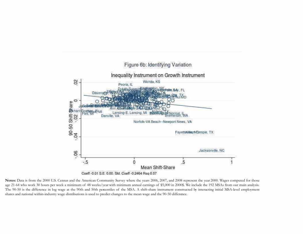
Notes: Data is from the 2000 U.S. Census and the American Community Survey where the years 2006, 2007, and 2008 represent the year 2000. Wages computed for those
age 21-64 who work 30 hours per week a minimum of 48 weeks/year with minimum annual earnings of $5,000 in 2000$. We include the 192 MSAs from our main analysis.
The 90-50 is the difference in log wage at the 90th and 50th percentiles of the MSA. A shift-share instrument constructed by interacting initial MSA-level employment
shares and national within-industry wage distributions is used to predict changes to the mean wage and the 90-50 difference.
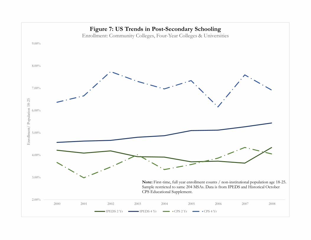
2.00%
3.00%
4.00%
5.00%
6.00%
7.00%
8.00%
9.00%
2000 2001 2002 2003 2004 2005 2006 2007 2008
En
rollm
ent/
Po
pula
tio
n 1
8-25
Figure 7: US T��DEF��D���F�-S�conda�y School�D�Enrollment: Community Colleges, Four-Year Colleges & Universities
IPEDS 2 Yr IPEDS 4 Yr CPS 2 Yr CPS 4 Yr
Not��First-time, full year enrollment counts / non-institutional population age 18-25. Sample restricted to same 204 MSAs. Data is from IPEDS and Historical October CPS Educational Supplement.

����%
10.00%
20.00%
30.00%
40.00%
50.00%
60.00%
70.00%
80.00%
90.00%
100.00%
18-25 migrants above 18-25 non-migrants above 18-25 migrants below 18-25 non-migrants below
Figure 8: Characteristics of MigrantsPeople Who Lived in Different MSA in Previous Year: Avg 2001 to 2008
%male %white %no college
Notes: Data is from the March CPS 2001-2008. Sample is restricted to non-institutional population age 18-25. We include the 135 MSAs used in anaysis of enrollments in the October CPS. Migrants identified as those not living in the same house or the same county in the prior year. "Above" ("below") denotes MSAs with values of the Gini instrument above (below) the median.

���������ABB�CD�E�EF�EF��
�����F������C��E�CF�EF��
�����F������C��E�CF�EF�� � ���� E����� �F� �� �� �� ���
�!� 1�� ������ ����� ������ ������ ������ ���� �����
"F�F��#�$$F�F��E� ��� ����A ����� ���� ����� ����� ���A� �����
%�&����F$$�C���� ��� ����� ���A ��A�A ����� ����A ���A� ���
'#!�(#)A��EF#� ��� ���� ����� ����� ������ ������ ������ ������
����*���C� ��� ����B ��CB ����B ���B ����B �����B C����B
+�B����,B)�#DB��E���C� ��� �����B A�C�B C���B �C���B ���A�B �����B ����B
'#-�.BBF!C��E���C� ��� ��A�B ��ACB ����B ����B ��C�B ��CCB �����B
(#)A��EF#����C��-FE���#���!��/EE�F�B��E�
F���%0� ��� ���CB C��B �AB �C�A�B �����B ���C�B ����CB
.(,��/��C�!���#BBA�FED��#���!��
,�C#��B��E��%%1�E#����� ��� A���B ����B ����B ����B C���B ��A�B �����B
.(,��/��C�!���#BBA�FED��#���!�������
,�C#��B��E��%%1�E#����� ��� C���B ���CB ���CB ���B C���B A���B �����B
.(,��/��C�!���#BBA�FED��#���!��
+�B����,�C#��B��E��%%1�E#����� ��� A���B ��A�B ����B ����B C���B ���B ����B
�(�/��C�!���#BBA�FED��#���!��
,�C#��B��E��%%1�E#����� ��A ��A�B ����B ��C�B ���CB ���CB C���B �����B
�(�/��C�!���#BBA�FED��#���!�������
,�C#��B��E��%%1�E#����� ��� C���B ��A�B ��CCB ����B ��C�B A���B ���AAB
�(�/��C�!���#BBA�FED��#���!��+�B����
,�C#��B��E��%%1�E#����� �� ���B ��CB ��AAB ����B ���AB C��B ���CAB
.(,��/��C�!��+#AC&2��C�,�C#��B��E�
�%%1�E#����� �� ����B C���B ����B ��B C��B ��CB �����B
.(,��/��C�!��+#AC&2��C������
,�C#��B��E��%%1�E#����� �� A��AB C�AB ����B ���CB C�A�B ����B �C��B
.(,��/��C�!��+#AC&2��C�+�B����
,�C#��B��E��%%1�E#����� �� ����B A���B ����B ����B A�CAB ����B ����B
�(�/��C�!��+#AC&2��C�,�C#��B��E��%%1�E#�
���� �A� ����B C�AB ���B C��AB ��AAB ����B �����B
�(�/��C�!��+#AC&2��C������,�C#��B��E�
�%%1�E#����� ��� ��ACB A�A�B ����B ����B ����B ���B �����B
�(�/��C�!��+#AC&2��C�+�B���,�C#��B��E�
�%%1�E#����� ��� ����B A��AB ����B C���B ���AB �����B �����B
3��F4��EF����!C�!�EF#������ ��� ����� ����� ����A ����� ���� ����� ����
3��F4��EF����!C�!�EF#��%�E��(�C���EF���
���� ��� ����C ���CC ����� ���� ����� ���A� ����C
3��F4��EF����!C�!�EF#����E��(�C���EF���
���� ��� ����� ����� ����C ����� ����� ����� �����
�#E����DEFE�������E���E��������A�����������������������������F�� ���!�!" EF�����# E�$��%E�������E ����! �&����%E���� ���������E�F��%E���E��������� ������"�EF�����%E�����������F%������������'�(��)���"����*���+��"E ��E�������!"F�������F%����E�������C���%�����$����%�"���!������$��E������"�����C����$�,&�E����F%������"��E��"E ��E E�&�-A������.�"�EF�����EFE���������F%��*�F���EF���/��F������E�&�.�"�EF����DEFE�(&�F���0*/.D(1�E���F%��2�F�#���("!! ����F����F%��)"����F�/�!" EF����("�+�&�0)/(1��*��F%��*/.D(��EFE������ ���F��EF�����E+��E�����+���&�E������C�F��������.��� ���F��EF���E����E �" EF���#&���E �������� ���F���"�F�������*/.D(�#&���F��!� EF���!�!" EF������"�F�������������F�F"F���E �!��! ��E�����F���A������F%��)���"��E���3)(� *��F%��)/(������ ���F��EF���E����E �" EF���#&����#������������EF���������4"��F�����E�$���E#�"F��" �F�������� ���F��FEF"����"����F�&�E�������%�� ��E���F&!� ������F�F"F�����5������F�"�F�����F�F������" �&�E������ ���F���"�F��#&���"�F����!��! ��E�����F���A��������F�&�E�������%�� �#&� �+� ����E��" �F����#E����E�����E ����#&�!�!" EF��������������F�F"F���E �!��! ��E�����F���A������F%��)/(� DEFE�"����F�����!"F��F%��������EF������E�"������������F%��6EF���E �7��F����E ������E!%���*�����EF����(&�F���067�*(1���6���%#��%�����������!����F��)���"��F�E�F��E���E���E�����EF���F��F%��8(3� �+� ��9� ������:�E������;���%����0����������1��������EF���������E�"����E��F%��:E�$2�����<%���&�*���=��%��%����E���E�"�������+����������F%���!EF�E ����F��#"F�����������+��"E ����F%����!��F�F����������3���E�"����������� ��F��!�����F���F���EF�����E���E�"����������� ��F��!�����F�������EF������
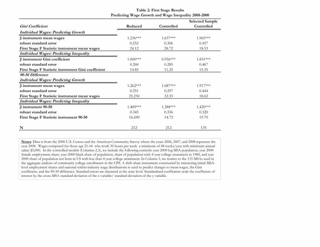
���������ABCD�ED�F����C��DC
�B��A�DA�F���F���B��D��������F���������AD������ ����
�A�A�!��""A�A��D ������� !��DB�����
E����D���E�#$���
!��DB�����
���A%A�������F�C���B��A�DA�F��B��D�
&�A�CDB�#��D�#������F�C 1.������ �������� �������
B���CD�CD����B���BB�B A��� A��A� A�B�
ABCD�ED�F���ED�DACDA��A�CDB�#��D�#������F�C �B��� �C��� �C��
���A%A�������F�C���B��A�DA�F��������AD�
&�A�CDB�#��D��A�A����""A�A��D ��AAA��� A������ ��C�����
B���CD�CD����B���BB�B A���A A��C A�B��
ABCD�ED�F���ED�DACDA��A�CDB�#��D��A�A����""A�A��D �B�C ���� ���
'� (��)A""�B����
���A%A�������F�C���B��A�DA�F��B��D�
&�A�CDB�#��D�#������F�C �������� ���C���� ��������
B���CD�CD����B���BB�B A��� A���� A�BBB
ABCD�ED�F���ED�DACDA��A�CDB�#��D�#������F�C ����A ����� �C���
���A%A�������F�C���B��A�DA�F��������AD�
&�A�CDB�#��D�'� (� ��BA���� ���CC��� ��B�A���
B���CD�CD����B���BB�B A��B A���� A���A
ABCD�ED�F���ED�DACDA��A�CDB�#��D�'� (� �����A �B��� ����A
* ��� ��� ��
*�D�CDEF���E��E����E���E�AAAE����E������E���E���E ����!��E��������"E���#�"E$����E���E"����E�AA�%E�AA�%E���E�AACE��&������E���E"���E�AAC�EE'�(��E!��&����E���E�����E�(�E��)�BEE$��E$��*E�AE�����E&��E$��*EE�E�������E��EBCE$��*�+"���E$���E�������E�����,E��,��"E-%AAA�EE.�E���E!�����,,��E����,�E/��,����E�%�0%E$�E��!,���E���E��,,�$��(E!�����,�DE"���E�AAAE,�(E1� E&�&�,�����%E"��� �AAAE����,�E��&,�"����E�����%E"���E�AAAE2,�!*E�����E��E&�&�,�����%E�����E��E&�&�,�����E$���EB)"���E!�,,�(�E����������E��E��CA%E���E"���E�AAAE�����E��E&�&�,�����E���E2���E��E��E$���E,���E����EB)"���E!�,,�(�E�����������E.�E��,���E�%E$�E������!�E��E���E��E1� �E����E��E���E�((��(���E���,"���E��E!�������"E!�,,�(�E����,,�����E��E���E�3��E E�����)�����E����������E!������!���E2"E������!���(E������,E1� ),�#�,E��&,�"����E������E���E�������,E$�����)�������"E$�(�E������2������E��E����E��E&����!�E!���(��E��E����E$�(��%E���E4���E!�����!����%E���E���E�A)AE��������!��E��������E������E���E!,�������E��E���E�����E,�#�,�E���������5��E!�����!�����E�!�,�E���E!�����!����E��E��������E2"E���E!����)1� E��������E��#������E��E���E6E#����2,�+E��������E��#������E��E���E"E#����2,��E
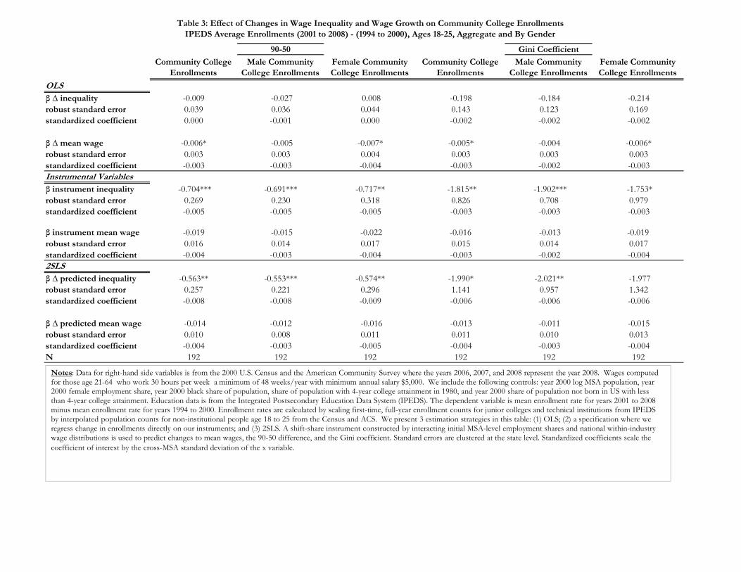
���������AA�BC�DA�EF����������������������C�������������D�CF�D��ED�����C��ED��������D�����C�
��� �!"��������D�����C��#$%%&�CD�$%%'(�)�#&**+�CD�$%%%(,�!����&')$-,�!������C������.��������
*%)-% �����ED�AA�B���C
ED�����C��ED������
��D�����C�
/����ED�����C��
ED��������D�����C�
0������ED�����C��
ED��������D�����C�
ED�����C��ED������
��D�����C�
/����ED�����C��
ED��������D�����C�
0������ED�����C��
ED��������D�����C�
12
3�4���������C� -0.00� ������� ������ ����� ����A ����A
�D���C��C����������D� ���B� ���BC ���AA ��AB ���B ��C�
�C�������5���BD�AA�B���C ����� ����� ����� ������ ������ ������
3�4���������� �����CD ������E ������D �����ED �����A �����CD
�D���C��C����������D� ����B ����B ����A ����B ����B ����B
�C�������5���BD�AA�B���C �����B �����B �����A �����B ������ �����B
���C�����C���6��������
3����C�����C���������C� ������ADDD ���C�DDD �����DD ����EDD ������DDD ����EBD
�D���C��C����������D� ���C� ���B� ��B� ����C ����� �����
�C�������5���BD�AA�B���C �����E �����E �����E �����B �����B �����B
3����C�����C���������� ����� �����E ������� ����C �����B �����
�D���C��C����������D� ���C ���A ���� ���E ���A ����
�C�������5���BD�AA�B���C �����A �����B �����A �����B ������ �����A
$ 2
3�4�7����BC�����������C� ���ECBDD ���EEBDDD ���E�ADD �����D �����DD ������
�D���C��C����������D� ���E� ���� ����C �A ���E� �BA�
�C�������5���BD�AA�B���C ������ ������ ������ �����C �����C �����C
3�4�7����BC������������ �����A ����� �����C ����B ���� ����E
�D���C��C����������D� ���� ����� ��� ��� ���� ���B
�C�������5���BD�AA�B���C �����A �����B �����E �����A �����B �����A
8 �� �� �� �� �� ��
8DC��F������������������������������������������ ����������!�"��#���$����������% ���&���#� $���'�"$���'�(���������'��������C)�����)������������*�����������'�����������+�����&� *$��������������������CA��(���(��,�B����$���*���(��,���� ��� $ ����A��(��,�-'����(���� ��� $ ����$��������'�.E)������+����&�$������������(����&�������F�'�������������/"%�*�*$������)�'����������� ����� *��' ���������)�'������������&,����������*�*$������)����������*�*$�������(����A�'����&������������� ����������)�����'������������������*�*$�������������������!"�(��������������A�'����&������������� �����0�$&����������������� �����1����������2�����&�����'�0�$&�����������"'��� �3120�"4��5�����*������������������� ���������� �������������'���� ������������ ��$�� ���������� �������������'�������A����������0����� ��������������&��&$�������'��&�������������� �)��$���'���������� ����&�$��������6$�����&��������������&���&���������$��������� �120�"��'������*�������*�*$�������&�$������������������$�������*��*�������������E���� �����#���$������%#"� +��*�������B����� ������������������������������F�34�78"9�3�4����*�&���&������(�����(����������&��������������� ���������&��'�����$�������$ ����9�����3B4��"8"��%������������������$ ����&�����$&�����'�������&�������������/"%�������� *��' ������������������������(���������$���'�(�����������$���������$�������*����&��&���������� ����(����)��������E����������&�)���������:����&�����&������"������������������ &�$���������������������������"��������;���&�����&�������&��������
&�����&������������������'�����&�����/"%���������������������������<�����������
���������AA�BCD�EA�F�����D�����������������C�������������E�C��E��FE�����C��FE��������E�����CD
��� �!"��������E�����CD�#$%%&�CE�$%''(�)�#'**��CE�$%%%(+�!��D�',)$&+�!������C���������������
*%)&% �����FE�AA�B���C
FE�����C��FE������
��E�����CD
-����FE�����C��
FE��������E�����CD
.������FE�����C��
FE��������E�����CD
FE�����C��FE������
��E�����CD
-����FE�����C��
FE��������E�����CD
.������FE�����C��
FE��������E�����CD
/0
1�2���������C� ����� ������� ����� ������ ������ ������
�E��DC�DC����������E� ���� ����A ����B ���C� ���� ����C
DC�������3���BE�AA�B���C ����� ������ ����� ������ ������ ������
1�2���������� �����CD �����D �����BD �����ED �����D �����CD
�E��DC�DC����������E� ����� ����� ����A ����� ����� �����
DC�������3���BE�AA�B���C �����A ������ �����A ������ ������ �����A
��DC�����C���4�������D
1���DC�����C���������C� ���C��DD ���EEBDD ����CE�D �����CD �����ADD �����BD
�E��DC�DC����������E� ���E ����B ����B ����B ����� �����
DC�������3���BE�AA�B���C ����� �����A ����� ������ ������ ������
1���DC�����C���������� �����E �����A �����B ������ ������ �����A
�E��DC�DC����������E� ����� ����C ����� ����� ����E �����
DC�������3���BE�AA�B���C �����A �����A ����� �����A ������ �����A
$ 0
1�2�5����BC�����������C� ����B�DD ����EADD �����ED ����CD ���ACEDD ������
�E��DC�DC����������E� ����� ����C ��� ��A�� ���CA ��E��
DC�������3���BE�AA�B���C ������ �����B ������ �����E �����E �����E
1�2�5����BC������������ �����C �����ED ������ �����C �����E �����B
�E��DC�DC����������E� ����� ����� ����� ����� ����� ����
DC�������3���BE�AA�B���C �����A �����A ����� �����A �����A �����
6 �B� �B� �B� �B� �B� �B�
6EC�DF������������������������������������������ ����������!�"��#���$����������% ���&���#� $���'�"$���'�(���������'��������)����E)��������C���*�����������'�������C���+�����&� *$������������������������(���(��,������$���*���(��,���� ��� $ �����C�(��,�-'����(���� ��� $ ����$��������'�.A)������+����&�$������������(����&�������F�'�������������/"%�*�*$������)�'����������� ����� *��' ���������)�'������������&,����������*�*$������)����������*�*$�������(������'����&������������� ��������BC�)�����'������������������*�*$�������������������!"�(����������������'����&������������� �����0�$&����������������� �����1����������2�����&�����'�0�$&�����������"'��� �3120�"4��5�����*������������������� ���������� �������������'��������A��������� ��$�� ���������� �������������'������BB�����������0����� ��������������&��&$�������'��&�������������� �)��$���'���������� ����&�$��������6$�����&��������������&���&���������$��������� �120�"��'������*�������*�*$�������&�$������������������$�������*��*��������C�����A���� �����#���$������%#"� +��*������������� ������������������������������F�3�4�78"9�3�4����*�&���&������(�����(����������&��������������� ���������&��'�����$�������$ ����9�����3�4��"8"��%������������������$ ����&�����$&�����'�������&�������������/"%�������� *��' ������������������������(���������$���'�(�����������$���������$�������*����&��&���������� ����(����)�����B��A�)���������:����&�����&������"�������������������&�$���������������������������"��������;���&�����&�������&��������&�����&������������������'�����&�����/"%���������������������������<�����������
���������AA�BCD�EA�F�����D�����������������C�������������E�C��E��FE�����C��FE��������E�����CD
F��� !��������E�����CD�"#$$%�CE�#$$&'�(�"%))*�CE�#$$$'�+� ��D�%&(#�+� ������C���������������
)$(�$ �����FE�AA�B���C
FE�����C��FE������
��E�����CD
,����FE�����C��
FE��������E�����CD
-������FE�����C��
FE��������E�����CD
FE�����C��FE������
��E�����CD
,����FE�����C��
FE��������E�����CD
-������FE�����C��
FE��������E�����CD
./�
0�1���������C� ����� ����� ������ ������ ���� ����
�E��DC�DC����������E� ���A� ��B� ��B� ����� ���� ��CB
DC�������2���BE�AA�B���C ����B ����D ����� �����B ����B �����
0�1���������� ������AEE ����B�EEE ����B� �����AE ����B�EE ����BC
�E��DC�DC����������E� ����� ����� ���B ����� ����� ���B
DC�������2���BE�AA�B���C ������ ����B� �����A ������ �����A �����D
��DC�����C���3�������D
0���DC�����C���������C� ������E ����ACD �B�CD�EE �����BEE ��� ��A���DEEE
�E��DC�DC����������E� ��D ���C� ���D� B���A ��BDC ���A�
DC�������2���BE�AA�B���C ����� ������ �����D ������ ������ ����B
0���DC�����C����������D ������� �������EE �����B ����B� �������EE ����C�
�E��DC�DC����������E� ���B� ����D ���CD ���BC ����A ���C
DC�������2���BE�AA�B���C �����C ����BB ����B� ����� ����B� �����D
#�/�
0�1�4����BC�����������C� �����A ���D�B �����BEE ���B��EEE ������E �C���BEEE
�E��DC�DC����������E� ����B ��D�C ���� ��DBC B���� ��A��
DC�������2���BE�AA�B���C ������ ����B ����BB ������ �����D ����BC
0�1�4����BC������������ ����B�EE �����D �����E ����BBE �����AE �����EE
�E��DC�DC����������E� ����� ����� ���BA ����� ���BD ���B�
DC�������2���BE�AA�B���C ������ ����B ����B� ����� ����B� ����B�
5 B� B�B A� B� B�B A�
5EC�DF������������������������������������������ ����������!�"��#���$����������% ���&���#� $���'�"$���'�(���������'���������)�����)��������D���*�����������'�������D���+�����&� *$�������������������B��C��(���(��,�����$���*���(��,���� ��� $ ����CD�(��,�-'����(���� ��� $ ����$��������'�.�)������+����&�$������������(����&�������F�'�������������/"%�*�*$������)�'����������� ����� *��' ���������)�'������������&,����������*�*$������)����������*�*$�������(����C�'����&������������� �������BAD�)�����'������������������*�*$�������������������!"�(��������������C�'����&������������� �����0�$&����������������� �����1������&���2&������0�$&��������"$**�� �����������#$������3�*$�������"$���'�4#3"5� 6�����*������������������� ���������� �������������'��������B�������D� ��$�� ���������� �������������'�����BAAC����������0����� ��������������&��&$�������'�&� ������������ ��������� �7$����������,������$���$����� �������� ��������$�)�&$������'��������&����)������'*�����������$������+��&�����$&���������� �)��$���'���������� ����&�$��������8$�����&��������������&���&���������$�������'�&�$������*��*�������BD����������������'��������&����������&� $���'�&�������������$����� �������������&�������'�*�*$��������������������$�������*��*�������BD���������� �����#3"� +����&�$���/"%��(�����$���&�������������������������������$�������*��*�������BD����(����&� *�������$&����������� �������+��*������������ ������������������������������F�4B5�29":�4�5����*�&���&������(�����(����������&��������������� ���������&��'�����$�������$ ����:�����45��"9"��%������������������$ ����&�����$&�����'�������&�������������/"%�������� *��' ������������������������(���������$���'�(�����������$���������$�������*����&��&���������� ����(����)�����A�������������&�)���������;����&�����&������"�������������������&�$���������������������������"��������<���&�����&�������&��������&�����&������������������'�����&�����/"%���������������������������=�
����������
���������AA�BCD�EA�F�����D�����������������C�������������E�C��E���E��������FE��������E�� ��CD
�!"#�$%��������E�� ��CD�&'(()�CE�'((*+���&),,-�CE�'(((+.�$��D�)*�'/.�$������C���������������
,(�/( �����FE�AA�B���C
-������FE������
��E�� ��CD
0����-������FE������
��E�� ��CD
�� ����-������FE������
��E�� ��CD
-������FE������
��E�� ��CD
0����-������FE������
��E�� ��CD
�� ����-������FE������
��E�� ��CD
12#
3�4���������C� ����1� ������ ������� ������� �����AB ����C�
�E��DC�DC����������E� ���A� ���D� ����� ����� ����� �����
DC�������5���BE�AA�B���C ������ ������ ����� ������ ������ �����D
3�4� �������� ���B� ���DE ���CB �����A ����D ������
�E��DC�DC����������E� ����� ����D ���A� ����� ����� �����
DC�������5���BE�AA�B���C ����� ����� ����D ����D ����� ����D
��DC�� ��C���6�������D
3���DC�� ��C���������C� ����A� ����BC ���EC ������C ����D�� ���ED�
�E��DC�DC����������E� ���B� ���A� ����B ���CB ����� ��C��
DC�������5���BE�AA�B���C ����� ������ ����� ������ ������ ������
3���DC�� ��C� ��������D ������� �����B ����D ������� �����B �����
�E��DC�DC����������E� ����B ����B ����� ����B ����B �����
DC�������5���BE�AA�B���C ����� ������ ����� ����� ������ �����
'#2#
3�4�7����BC�����������C� �����DC ������B ����� ����EC� ����EA ����D�
�E��DC�DC����������E� ����E ���DC ���A� ��B�E ����B �����
DC�������5���BE�AA�B���C ������ ������ ����� �����D �����D ������
3�4�7����BC��� �������� ������� �����A ����� ������ �����A ������
�E��DC�DC����������E� ����D ����A ����D ����A ����B ����A
DC�������5���BE�AA�B���C ����� ������ ����� ����� ������ �����
8 �EC �EC �EC �EC �EC �EC
8EC�DF������������������������������������������ ����������!�"��#���$����������% ���&���#� $���'�"$���'�(���������'���������)����C)��������E���*�����������'�������E���+�����&� *$����������������������A��(���(��,�D����$���*���(��,���� ��� $ ����AE�(��,�-'����(���� ��� $ ����$��������'�.B)������+����&�$������������(����&�������F�'�������������/"%�*�*$������)�'����������� ����� *��' ���������)�'������������&,����������*�*$������)����������*�*$�������(����A�'����&������������� ���������E�)�����'������������������*�*$�������������������!"�(��������������A�'����&������������� �����0�$&����������������� �����1����������2�����&�����'�0�$&�����������"'��� �3120�"4��0�$&����������������� �����1����������2�����&�����'�0�$&�����������"'��� �3120�"4��5�����*������������������� ���������� �������������'����������������E� ��$�� ���������� �������������'��������A����������0����� ��������������&��&$�������'��&�������������� �)��$���'���������� ����&�$��������������$�������(���������&����������������� �120�"��'������*�������*�*$�������&�$������������������$�������*��*��������E�����B���� �����#���$������%#"� +��*�������D����� ������������������������������F�3�4�67"8�3�4����*�&���&������(�����(����������&��������������� ���������&��'�����$�������$ ����8�����3D��"7"��%������������������$ ����&�����$&�����'�������&�������������/"%�������� *��' ������������������������(���������$���'�(�����������$���������$�������*����&��&���������� ����(����)��������B�)���� ����9����&�����&������"�������������������&�$���������������������������"��������:���&�����&�������&��������&�����&������������������'�
����&�����/"%���������������������������;�����������

���������AA�BCD�EA�F�����D�����������������C�������������E�C��E���E��������FE��������E�� ��CD
�!"#�$%��������E�� ��CD�&'(()�CE�'(**+���&*,,-�CE�'(((+.�$��D�*/�').�$������C������0��������
,(�)( �����FE�AA�B���C
-������FE������
��E�� ��CD
1����-������FE������
��E�� ��CD
�� ����-������FE������
��E�� ��CD
-������FE������
��E�� ��CD
1����-������FE������
��E�� ��CD
�� ����-������FE������
��E�� ��CD
23#
4�5���������C� ������ ����1� ����� ������ ���1�� ���A�B
�E��DC�DC����������E� ���A� ����� ���BA ���B� ����� �����
DC�������6���BE�AA�B���C ����� ������ ����� �����A ������ �����B
4�5� �������� ����� ����B ����C ����� ����� �����
�E��DC�DC����������E� ����� ����� ����A ����� ����� ����A
DC�������6���BE�AA�B���C ����A ����A ����B ����B ����A �����
��DC�� ��C���7�������D
4���DC�� ��C���������C� �����C ������ ���B� ����D� ����B� �����A
�E��DC�DC����������E� ����C ���CA ����� ��DBD ����C ����A
DC�������6���BE�AA�B���C ����� ������ ����� ������ �����A ������
4���DC�� ��C� �������� ������ ������ ����A �����A ������ �����
�E��DC�DC����������E� ����� ����� ����D ����� ����� ����D
DC�������6���BE�AA�B���C ����� ������ ����� ������ ������ �����
'#3#
4�5�8����BC�����������C� �����D ����CA ����A ����B� �����C ������
�E��DC�DC����������E� ����� ���C� ���D� ���C� ���AA ����A
DC�������6���BE�AA�B���C ����� ������ ����� �����A �����B ������
4�5�8����BC��� �������� ������ ������ ����� ������ ������ �����
�E��DC�DC����������E� ����B ����� ����� ����� ����C �����
DC�������6���BE�AA�B���C ����� ������ ����� ������ ������ �����
9 ��� ��� ��� ��� ��� ���
9EC�DEF����F���F����������F����F���������F��F��� F���F����F!�"�F#���$�F���F���F% ���&��F#� $���'F"$���'F(����F���F'����F���C)F����)F���F����F��*������F���F'���F�����FF+����F&� *$���F���F�����F���F���CBFF(��F(��,FA�F��$��F*��F(��,FF�F ��� $ F��FB�F(��,�-'���F(���F ��� $ F���$��F�����'F.�)����FF+�F��&�$��F���F�����(���F&�������EF'���F����F���F/"%F*�*$������)F'���F����F�� ���F� *��' ���F�����)F'���F����F���&,F�����F��F*�*$������)F�����F��F*�*$������F(���FB�'���F&������F������ ���F��F�D��)F���F'���F����F�����F��F*�*$������F���F����F��F!"F(���F����F����FB�'���F&������F������ ����F0�$&�����F����F��F��� F���F1���������F2�����&�����'F0�$&�����F����F"'��� F3120�"4�F0�$&�����F����F��F��� F���F1���������F2�����&�����'F0�$&�����F����F"'��� F3120�"4�F5��F��*������F��������F��F ���F������ ���F����F���F'����F����F��F����F ��$�F ���F������ ���F����F���F'����F�DDBF��F�����F0����� ���F�����F���F&��&$�����F�'F�&�����F�������� �)F�$���'���F������ ���F&�$���F���F������$�����F�(������F��&�����F�������F��� F120�"FF�'F�����*������F*�*$������F&�$���F���F����������$������F*��*��F���F��F��F��F��� F���F#���$�F���F%#"� +�F*������FAF���� �����F����������F��F����F�����EF3�4F67"8F3�4F�F�*�&���&�����F(����F(�F�������F&�����F��F������ ����F����&��'��F�$�F�����$ ����8F���F3AF�"7"�F%F�����������F�����$ ���F&�����$&���F�'F������&����F�������F/"%������F� *��' ���F������F���F��������F(���������$���'F(���F�������$�����F��F$���F��F*����&�F&������F��F ���F(����)F���FD����)F���F���F9���F&�����&�����F"�������F������F���F&�$������F��F���F�����F������F"��������:��F&�����&�����F�&���F���F&�����&����F��F��������F�'F���F
&�����/"%F��������F���������F��F���F;F���������F
���������AA�BCD�EA�F�������C��������E�C��E����D����C�����������C�E��
���������������C�E�
���������������C�E��
����BC������ �� ���������������C�E�
���������������C�E��
����BC������ ��
�!�
"�#���������C� ������� ����� ����� ����
�E��DC�DC����������E� ���AB ����� ����� �����
DC�������$���BE�AA�B���C ���CB ����� ����� ���AB
"�#����������� D������ D������ D����� D�����
�E��DC�DC����������E� ����� ����� ����� �����
DC�������$���BE�AA�B���C D����� D���� D����A D����C
F�DC�����C���%�������D
"���DC�����C���������C� ��C�A��� ������ ���B���� ������
�E��DC�DC����������E� ���A� ���� ���AA �����
DC�������$���BE�AA�B���C ���C� ���CA ���A� �����
"���DC�����C���������� D����B� D����A D���� D�����
�E��DC�DC����������E� ����� ����A ����� ����A
DC�������$���BE�AA�B���C D���� D����A D���C� D���A
&�!�
"�#� ����BC�����������C� ��C��� ������ ���C�� ���C�
�E��DC�DC����������E� ����� ����B ����� �����
DC�������$���BE�AA�B���C ����� ���C� ���C� ���C�
"�#� ����BC������������ D����� D����� D����� �����
DC����������E� ����� ����� ����� �����
DC�������$���BE�AA�B���C D����� D���C� D����B D�����
' ��� ��A ��� ��A
�����(E�AA�B���C )*+,*
'EC�D��EF���������������������������������� !���"������#��F��#�$F�DF�������������#�%��F�������&� ��'�����������F��!%�#�����'�%%����(� �#)�(�*F�#���F��(��#�����C+����+��������B�#��#�������F��(��#����B���,���)������*�$�����%��������#��F�����$����DC���*F��*�#-����F��#����#�*��-����%���%�%�����B�*��-�.(��#�*��F�%���%�%������������#(�/A+�����0�����������F�������*��$�����#���1�(��#��������$�� !�����������+�(��#����������-��F�#���������������+��F�#����������������*��F��D(��#������$��������%���������B�+�����(��#�������F�#����������������������#�����& �*��F�������F����D(��#������$��������%�����"��������������%������F����$#�$������%����#�������#�%��F��2��������3����#�����4��$#��F���,���#%������ (���%�5234, 6���2��$F��#F�������##����������'�������#����������#���$$#�$���������F��� !D��)����7����*��$�8��#���+�9���F����5����+�����6+���$#�$���������%����#�������F��8��-�:#��#�EF��#(�,���;�*F��F������%����#������)�����������F��������������#���������������)�������*��F�#��������������%���!�%����#������ #����������#���������$#�����+���%����#�������#����������#�������$#�$�������0���#������������%��������#���$��������F��������1�5�6�:< =�5�6�����������������*F�#��*��#�$#�����F��$�������#���%�������#����(������#�����#�%����=�����5�6�� < ��!��F���D�F�#������#�%���������#�������(�����#�����$���������� !D��)����%���(%�����F�#����������������*��F��D������#(�*�$������#���������������������#�������F��$������%����*�$��+��F����DA�+������F��4����������������� �����#���##�#���#��������#�������F����������)���� �����#��>�����������������������F���������������������#�����(��F��#���������F���#���D� !�������#����)�����������F��;�)�#����������F���#���D� !�������#����)�����������F��(�)�#�������

���������
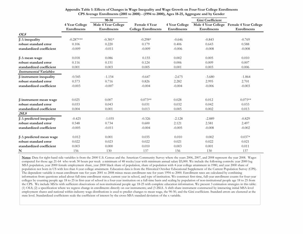
���������ABC��DE�F������������A���������A��������AC����A����A������������� ���!"�A����CC����F���CC#����
�$%��&��A���F���CC#�����'())D����())*+�!�'D,,-����()))+.������D*!(/.�������A���A���B��������
,)!/) ����������������
-�"�A����CC����
F���CC#����
0AC��-�"�A����CC����
F���CC#����
�#AC��-�"�A��
��CC����F���CC#����
-�"�A����CC����
F���CC#����
0AC��-�"�A����CC����
F���CC#����
�#AC��-�"�A����CC����
F���CC#����
12%
3�4������AC��� ��������� ������ ����A�� B���CDC ����D� ����CA
��B������A��A�������� ���C ����� ���A ��D�C ��CD� ��E��
��A��A���5�������������� �����A ���� �����A �����C ������ ������
3�4�#�A���A�� ���� ����C B��EE ����� ����E ����
��B������A��A�������� ��C ��E ���D ����C ����A �����
��A��A���5�������������� ���� ����� ����E ���� ����� ����C
������#���AC�6A��ABC��
3�������#���������AC��� ���EDE ��ED ���CD� B���C�E B���C�� B���CD
��B������A��A�������� ��E�� ���C ����C ����� ��AAE ����
��A��A���5�������������� ������ ������ �����D �����D �����C ������
3�������#����#�A���A�� ����E ����� B������� ����� ���� B����E��
��B������A��A�������� ����� ���D� ���� ����� ���D� �����
��A��A���5�������������� ����D ���� ���� ����E ����� ����
(%2%
3�4����������������AC��� B���D�E B����E �����C B����� B�����A �����A
��B������A��A�������� ��ED� ����D ��C�� ��� ��E� ��DA�
��A��A���5�������������� �����E ���� �����D �����E ������ ������
3�4�����������#�A���A�� B���� ���� ����E B���� B����� ������
��B������A��A�������� ����� ����� ����� ���� ����� ����
��A��A���5�������������� ����� ����� ���� ����� ���� ���
7 EC �� �� EC �� ��
7����FB����B���B����������B����B���������B��B��� B���B����B!�"�B#���$�B���B���B% ���&��B#� $���'B"$���'B(����B���B'����B���C)B����)B���B����B��*������B���B'���B�����BB+����B&� *$���B���B�����B���B��CDBB(��B(��,B��B��$��B*��B(��,BB�B ��� $ B��BD�B(��,�-'���B(���B ��� $ B���$��B�����'B.E)����B+�B��&�$��B���B�����(���B&�������FB'���B����B���B/"%B*�*$������)B'���B����B�� ���B� *��' ���B�����)B'���B����B���&,B�����B��B*�*$������)B�����B��B*�*$������B(���BD�'���B&������B������ ���B��BA��)B���B'���B����B�����B��B*�*$������B���B����B��B!"B(���B����B����BD�'���B&������B������ ����B0�$&�����B����B��B��� B���B1������&��B2&�����B0�$&�������B"$**�� ���B��B���B#$�����B3�*$������B"$���'B4#3"5�B6��B��*������B��������B��B ���B������ ���B����B���B'����B���B��B����B ��$�B ���B������ ���B����B���B'����BAADB��B�����B0����� ���B�����B���B&��&$�����B�'B&� ������B����� �����B��� B7$�������B��,��B���$�B�$����� �B������ ���B����$�)B&$�����B'���B��B�&����)B���B�'*�B��B������$�����B+�B&�����$&�B�������� �)B�$���'���B������ ���B&�$���B���B��$��'���B&�������B�'B&�$�����B*��*��B���B�B��B�EB��B������'���B��B�&����B��B�B��$��'���B������$����B��B�B�$����� �B�����B���B�&�����B�'B*�*$������B��B����������$������B*��*��B���B�B��B�EB��� B���B#3"� +�B��&�$��B/"%�B(���B�$���&����B������������B��B����������$������B*��*��B���B���EB(���B&� *����B��$&�����B����� ������B+�B*������B�B���� �����B����������B��B����B�����FB45B28"9B4�5B�B�*�&���&�����B(����B(�B�������B&�����B��B������ ����B����&��'B��B�$�B�����$ ����9B���B4�B�"8"�B%B�����������B�����$ ���B&�����$&���B�'B������&����B�������B/"%������B� *��' ���B������B���B��������B(���������$���'B(���B�������$�����B��B$���B��B*����&�B&������B��B ���B(���)B���BA��E�)B��� ���B:���B&�����&�����B"�������B������B���B&�$������B��B���B�����B������B"��������;��B&�����&�����B�&���B���B&�����&����B��B��������B�'B���B&�����/"%B��������B���������B��B���B<B���������B
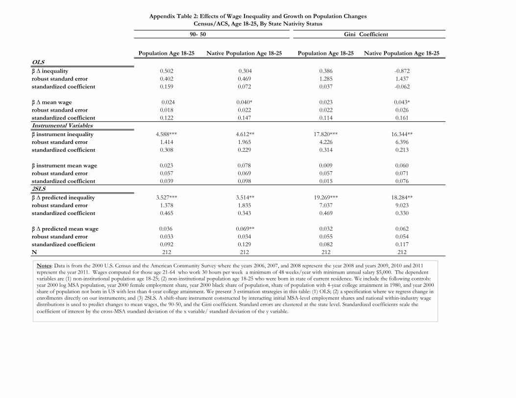
���������ABC��DE�F�����������A��������AC����A�����������������CA����� �A����
�����!� "#�����$%&D'#�(��"�A���)A��*����"�A���
+,& ', ����� ����������
����CA���������$%&D' )A��*������CA���������$%&D' ����CA���������$%&D' )A��*������CA���������$%&D'
-."
/�0������AC��� ����� ������ ���� A���B�
��B������A��A�������� ����� ���C D���� D���B
��A��A���1�������������� ��D�C ���B� ����B A����
/�0�2�A���A�� ������� �����E ����� �����E
��B������A��A�������� ���D� ����� ����� ����
��A��A���1�������������� ��D�� ��D�B ��DD� ��DD
������2���AC�3A��ABC��
/�������2���������AC��� �����EEE ���D�EE DB����EEE D����EE
��B������A��A�������� D��D� D�C� ���� ��C
��A��A���1�������������� ����� ����C ���D� ���D�
/�������2����2�A���A�� ����� ���B� ����C ����
��B������A��A�������� ����B ���C ����B ���BD
��A��A���1�������������� ����C ���C� ���D� ���B
D"."
/�0����������������AC��� ����BEEE ����D�EE DC��CEEE D�����EE
��B������A��A�������� D��B� D���� B���B C����
��A��A���1�������������� ���� ����� ���C �����
/�0�����������2�A���A�� ����� ����CEE ����� ����
��B������A��A�������� ����� ����� ����� �����
��A��A���1�������������� ���C� ��D�C ����� ��DDB
) �D� �D� �D� �D�
)����F������������������������������������� �����!����"�����������#����$�#�%���������#��������&����B&��� ��������'�����������#��� ������� �#��������C&���D���� ���DD���'�����������#������DD���(�)���"��'��� ������������)���DA���%���%��*����������'���%��*������������������%��*�+#����%�����������������,���,��#�-�&������.��� �'�� ����$����/,�������0D1����A������������,�'�'�,�������)��D�A��2�0�1����A������������,�'�'�,�������)��D�A���%���%����/����������������"����������� ��"���(����",� ��������,,�%��)�"�����,�F�#���������,�)�3�!�'�'�,�����&�#�������������,����',�#����������&�#���������/,�"*����������'�'�,�����&����������'�'�,������%�����A#����"�,,�)����������������DC��&��� �#������������������'�'�,����������/����������%����,����������A#����"�,,�)��������������(��'��������������������������)��������������/,�F�0D1�45�2�0�1����'�"���"������%�����%����)�����"���)���������,,������ ���"�,#�������������������2��� �0�1���5���!������A�����������������"������"�� �/#�������"���)�������,�3�!A,�$�,���',�#�������������� ��������,�%�����A�� ����#�%�)�� �����/������������� ����'�� �"��"���)�����������%�)��&�����C�A��&��� �����6����"�����"���������� �� ������������",������ ��������������,�$�,������ �� �7� �"�����"�������"�,������
"�����"�����������������/#�����"����A3�!����� �� � �$��������������8�$����/,�+����� �� � �$��������������#�$����/,���