risk analysis & modelling lecture 5: value at risk & solvency ii
TRANSCRIPT
Risk Analysis & Modelling
Lecture 5: Value at Risk & Solvency II


Making Sense of Quantitative Risk
In an earlier lecture we looked at the Mean-Variance ModelWe saw how we could calculate the Mean and Variance of the return on a portfolio using the Covariance Matrix, the Expected Returns and the Investment WeightsThe Expected Return was relatively easy to interpretThe Variance or Standard Deviation was abstract and could only be used to give a measure of the relative risk – the higher the Variance the higher the Risk

Value At Risk: Implying Potential Loss
People intuitively try to assess Risk in terms of worst case scenariosInformation on how much you could lose on a portfolio over the next day, month or year makes much more sense to most people than an abstract statistic such a varianceValue at Risk originated in the RiskMetrics group at the investment bank JP Morgan in the early 1990sIt quantifies the worst case scenario in terms of the probability of observing outcomes worse than this scenario (ie the Quantile of the loss)VaR is very closely related to the Probable Maximum Loss (PML) used to measure Underwriting Risks

Value At Risk
Random Asset Value
Increases in Values(Profit)
Decreases in Values(Loss)
Losses due to Random Movements in the Assets Value will only be greater than this some % of the
time
% Value at Risk

Measuring VaR From Historical Observations
Imagine we have some historical data (or simulated values) on the profits and losses experienced on an investment over a one year periodWe believe that this historical data represents the future profits and losses we might experienceWe could estimate the 5% VaR over the next year by locating the loss such that only 5% of the losses are worse (5% Empirical Quantile)We could estimate the 1% VaR over the next year by locating the loss such that only 1% of the losses are worse (1% Empirical Quantile)VaR is often calculated using statistical distributions…
VaR Assumption: Normally Distributed Returns
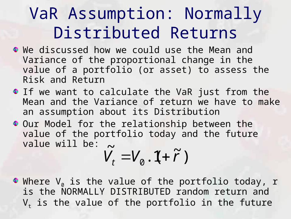
We discussed how we could use the Mean and Variance of the proportional change in the value of a portfolio (or asset) to assess the Risk and ReturnIf we want to calculate the VaR just from the Mean and the Variance of return we have to make an assumption about its DistributionOur Model for the relationship between the value of the portfolio today and the future value will be:
Where V0 is the value of the portfolio today, r is the NORMALLY DISTRIBUTED random return and Vt is the value of the portfolio in the future
)~1.(~
0 rVVt

The Value at Risk Model
0V
r~
0
0.05
0.1
0.15
0.2
0.25
0.3
0.35
0.4
0.45
0.5
-3 -2 -1 0 1 2 3
Pro
ba
bil
ity
De
ns
ity
)~1.(01 rVV

Since Value at Risk tries to measure the maximum loss we need to convert this into a model of the profit or loss
The random profit or loss (P) on holding an asset can be defined as:
The Value at Risk is simply the value that P will only go below some percentage of the time
This value can be calculated by finding the appropriate Quantile for the Normally Distributed random return r
0000 .~)~1.(~~
VrVrVVVP t

Calculating VaR from the Return
r~
rVP ~.~
0
0
0.05
0.1
0.15
0.2
0.25
0.3
0.35
0.4
0.45
0.5
-3 -2 -1 0 1 2 3
Pro
ba
bil
ity
De
ns
ity
By finding the value that Returns will be less than or equal to 5% of the time we can calculate the value
negative losses will be less than or equal to 5% of the time or the 5% VaR
0
0.05
0.1
0.15
0.2
0.25
0.3
0.35
0.4
0.45
0.5
-3 -2 -1 0 1 2 3
Pro
ba
bil
ity
De
ns
ity
P~

Example VaR CalculationThe average return on the portfolio over the next year is 4% and the standard deviation is 7%If we assume returns are Normally Distributed, we can use NORMINV to calculate the value that the annual return will be less than or equal to 5% of the time (the 5% Quantile):
=NORMINV(0.05,0.04,0.07)This gives us a value of -0.07514 (-7.514%)If the initial value of the portfolio was £10000 then the loss for this return would be -£751.4 (-0.07514 * 10000) over the next year5% of the time we will observe losses more severe than -£751.4 - this is the 5% VaR on the portfolio

5% VaR Calculation Diagram
0
0.1
0.2
0.3
0.4
0.5
0.6
0.7
0.8
0.9
1
-0.15 -0.1 -0.05 0 0.05 0.1 0.15 0.2
CDF of returns with = 0.04 and = 0.07
0.05
-0.07514
Only observe returns less than this 5% of the
time
5% VaR = -0.07514 * 10000 = -£751.4

VaR Review Question
The annual return on the portfolio is Normally Distributed with an Average of 6% and a Standard Deviation of 10%
The initial value of the portfolio is £250,000
Calculate the 5% VaR over a 1 year horizon
Calculate the 1% VaR over a 1 year horizon
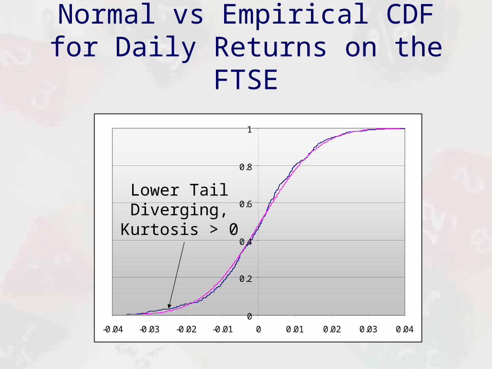
Normal vs Empirical CDF for Daily Returns on the FTSE
0
0.2
0.4
0.6
0.8
1
-0.04 -0.03 -0.02 -0.01 0 0.01 0.02 0.03 0.04
Lower Tail Diverging,
Kurtosis > 0
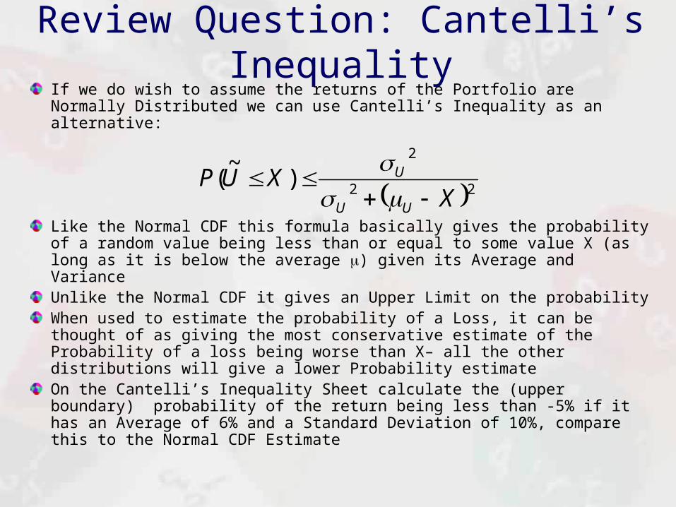
Review Question: Cantelli’s InequalityIf we do wish to assume the returns of the Portfolio are Normally Distributed we can use Cantelli’s Inequality as an alternative:
Like the Normal CDF this formula basically gives the probability of a random value being less than or equal to some value X (as long as it is below the average ) given its Average and VarianceUnlike the Normal CDF it gives an Upper Limit on the probabilityWhen used to estimate the probability of a Loss, it can be thought of as giving the most conservative estimate of the Probability of a loss being worse than X– all the other distributions will give a lower Probability estimateOn the Cantelli’s Inequality Sheet calculate the (upper boundary) probability of the return being less than -5% if it has an Average of 6% and a Standard Deviation of 10%, compare this to the Normal CDF Estimate
22
2
)~
(X
XUPUU
U

Locating Quantiles for the Normal Distribution
One useful feature of the Normal Distribution is its Quantiles can be located by simply taking a number of Standard Deviations from the AverageFor example, the 5% Quantile for a Normally Distributed random variable is located 1.645 Standard Deviations below the AverageThe 1% Quantile for a Normally Distributed random variable is located 2.326 Standard Deviations below the AverageThe 0.5% Quantile of a Normally Distributed random variable is located 2.575 Standard Deviations below the AverageThe number of Standard Deviations below the Average can be calculated using the CDF of a Standard Normal random Variable (Mean 0 and Standard Deviation of 1)
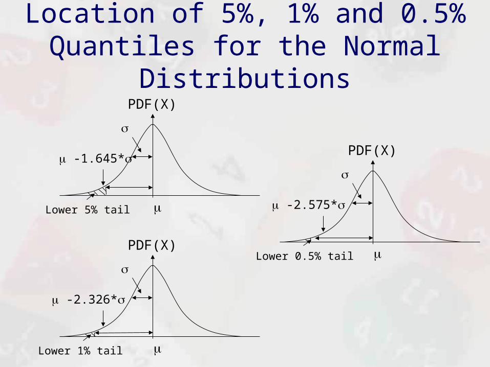
Location of 5%, 1% and 0.5% Quantiles for the Normal Distributions
Lower 5% tail
-1.645*
PDF(X)
Lower 1% tail
-2.326*
PDF(X)
Lower 0.5% tail
-2.575*
PDF(X)

5% Quantile for Normal Distribution with = 0.04 and = 0.07
0
0.1
0.2
0.3
0.4
0.5
0.6
0.7
0.8
0.9
1
-0.15 -0.1 -0.05 0 0.05 0.1 0.15 0.2
0.04 – 1.645 * 0.07 = -0.07515
0.05
The location of the 5% Quantile is 1.645 standard deviation below the mean

VaR Formula
To calculate the 5% VaR over some time horizon we can simply apply
VaR5%=V0.(-1.645*)
Where V0 is the initial value of the portfolio or asset, is the mean of random return over the period and is the standard deviation over the period
The 1% VaR formula is equal to:
VaR1%=V0.(2.326*)
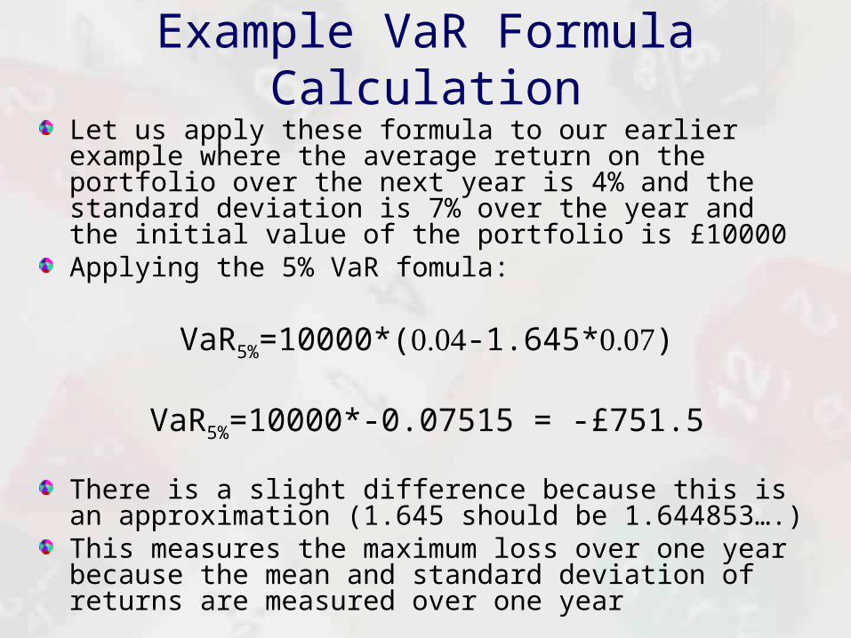
Example VaR Formula CalculationLet us apply these formula to our earlier example where the average return on the portfolio over the next year is 4% and the standard deviation is 7% over the year and the initial value of the portfolio is £10000Applying the 5% VaR fomula:
VaR5%=10000*(-1.645*)
VaR5%=10000*-0.07515 = -£751.5
There is a slight difference because this is an approximation (1.645 should be 1.644853….)This measures the maximum loss over one year because the mean and standard deviation of returns are measured over one year

Positive and Negative VaRSo far we have been calculating VaR as a negative value (signifying loss)
In practice it is often quoted as a positive number
This is achieved by multiplying the negative VaR formula by minus one:
VaR+X%=V0.(c*)
Where c is the desired confidence interval (c = 1.645 for 5% VaR)
For the rest of the lecture we will use this VaR+ measure since this in the convention

Absolute vs Relative VaR FormulaSo far our VaR calculation has measured the worst outcome by taking a number of Standard Deviations away from the Average, this is known as Absolute VaR:
This formula was based on the definition of Absolute Profit and Loss on an asset:
The formula for Relative Profit and Loss is relative to the expected FUTURE value of the investment:
0
~VVP tAbsolute
)~
(~
Re ttlative VEVP
rrAbsolute cVVaR ..0
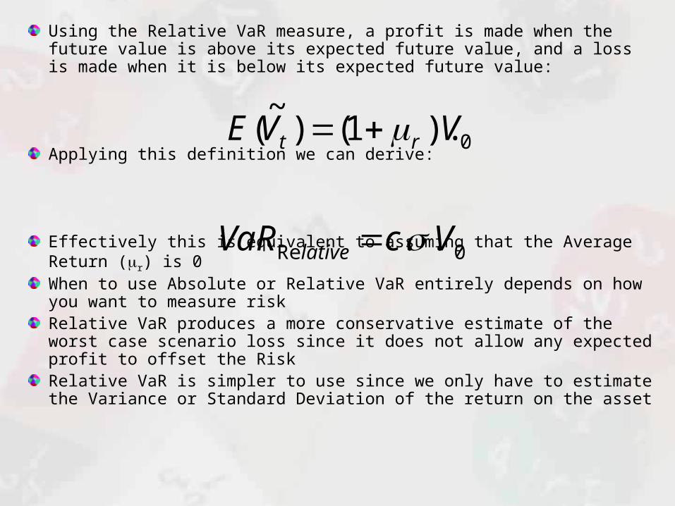
Using the Relative VaR measure, a profit is made when the future value is above its expected future value, and a loss is made when it is below its expected future value:
Applying this definition we can derive:
Effectively this is equivalent to assuming that the Average Return (r) is 0When to use Absolute or Relative VaR entirely depends on how you want to measure riskRelative VaR produces a more conservative estimate of the worst case scenario loss since it does not allow any expected profit to offset the RiskRelative VaR is simpler to use since we only have to estimate the Variance or Standard Deviation of the return on the asset
0Re .. VcVaR lative
0).1()~
( VVE rt
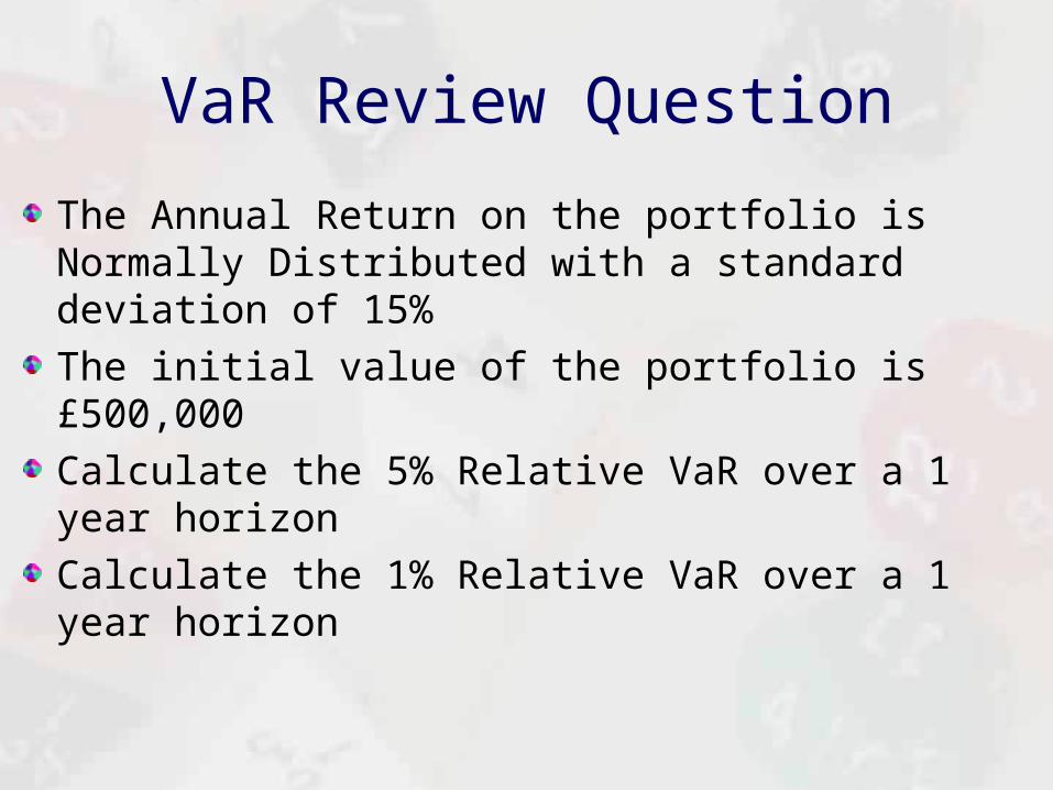
VaR Review Question
The Annual Return on the portfolio is Normally Distributed with a standard deviation of 15%
The initial value of the portfolio is £500,000
Calculate the 5% Relative VaR over a 1 year horizon
Calculate the 1% Relative VaR over a 1 year horizon
Conditional Value at Risk (CVaR)
Another Measure of Value at Risk is CVaR or Conditional Value at Risk (also known as ETL or Expected Tail Loss and ES or Expected Shortfall)
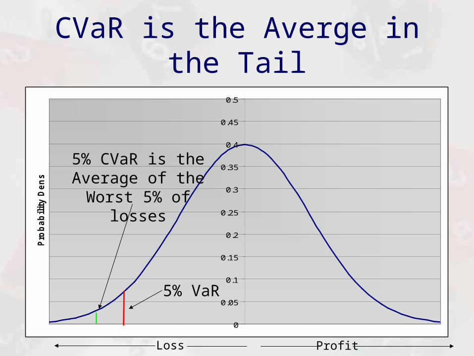
It measures the average of all the losses beyond some Quantile - for example the average of the worst 1% or 0.5% of losses
The estimate of the worst case scenario loss provided by CVaR is always greater than the VaR for a given level of confidence
CVaR has a number of advantages over traditional VaR
CVaR is the Averge in the Tail
0
0.05
0.1
0.15
0.2
0.25
0.3
0.35
0.4
0.45
0.5
-3 -2 -1 0 1 2 3
Pro
ba
bil
ity
De
ns
ity
5% VaR
5% CVaR is the Average of the Worst
5% of losses
ProfitLoss

Calculating CVaR for the Normal Distribution
)*1(
)(
cCDF
cPDFc
SN
SN
We can calculate CVaR for the Normal Distribution with by simply adjustment to the confidence interval c (c would be 1.64 for 5% VaR):
Where PDFSN and CDFSN is the Probability Density Function and Cumulative Distribution Function for the Standard Normal (Normal with mean 0 and standard deviation of 1)
We then apply this adjust confidence interval to standard VaR formula to obtain the equivalent CVaR:
.. 0Re VcCVaR lative

058.2),1,0,64.1*1(
),1,0,64.1(
TRUENORMDIST
FALSENORMDISTc
For example, if we want to find the confidence interval for the 5% CVaR we can take the 5% VaR interval (1.64) and apply the adjustment:
We could then see that the 5% Relative CVaR formula would be:
REVIEW QUESTION: Calculate the CVaR 0.5% confidence interval based on the VaR 0.5% confidence interval of 2.575 then calculate the Relative CVaR 0.5% for a portfolio with an initial value of £10000 and a standard deviation of 0.07
**058.2 0%5 VCVaR

Advantages of CVaR over VaRBoth VaR and PML (Probable Maximum Loss) are based on estimating the location of a single QuantileUnlike CVaR and ETL they do not take into account what is taking place beyond that Quantile and this can lead to problems when used with the Heavy Tailed Distributions used to model Extreme or Catastrophic LossesThe first problem with VaR and PML is that when used to measure potentially Catastrophic (Heavy Tail) Losses they can be very sensitive to small changes in the confidence intervalCVaR and ETL are less sensitive because they are not just based on a single loss but the average of losses beyond a valueAn example to highlight this sensitivity can be found on the “PML vs ETL” spreadsheet
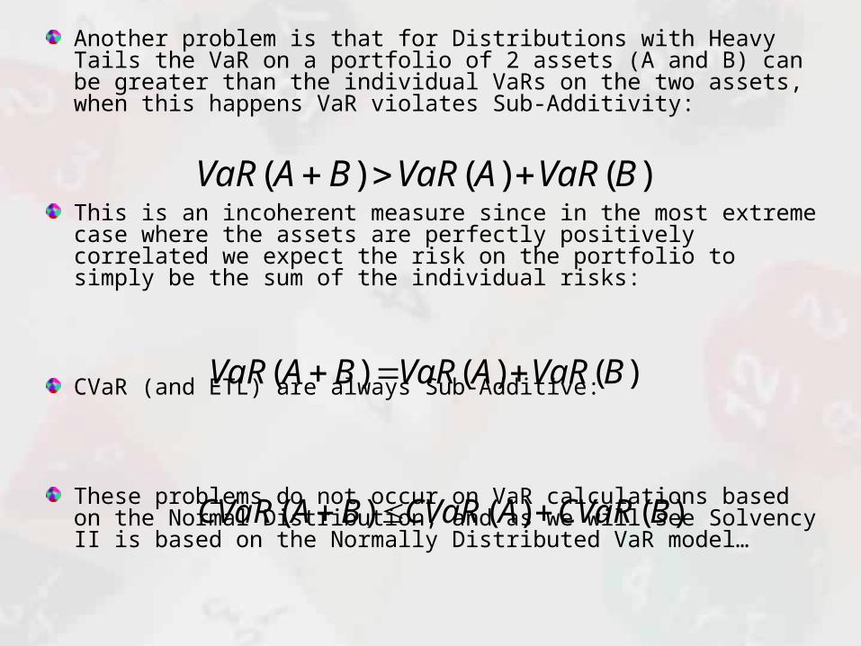
Another problem is that for Distributions with Heavy Tails the VaR on a portfolio of 2 assets (A and B) can be greater than the individual VaRs on the two assets, when this happens VaR violates Sub-Additivity:
This is an incoherent measure since in the most extreme case where the assets are perfectly positively correlated we expect the risk on the portfolio to simply be the sum of the individual risks:
CVaR (and ETL) are always Sub-Additive:
These problems do not occur on VaR calculations based on the Normal Distribution, and as we will see Solvency II is based on the Normally Distributed VaR model…
)()()( BVaRAVaRBAVaR
)()()( BCVaRACVaRBACVaR
)()()( BVaRAVaRBAVaR

VaR and the Mean Variance Framework
One of the main uses of VaR is to estimate the Risk on a Portfolio of Assets
To calculate a Portfolio’s Relative VaR we only have to calculate the Variance of its Return
In Lecture 2 we saw that this can be calculated as:
wCwTP ..2
wCwVcVcVcVaR TpPlative ........ 02
00Re
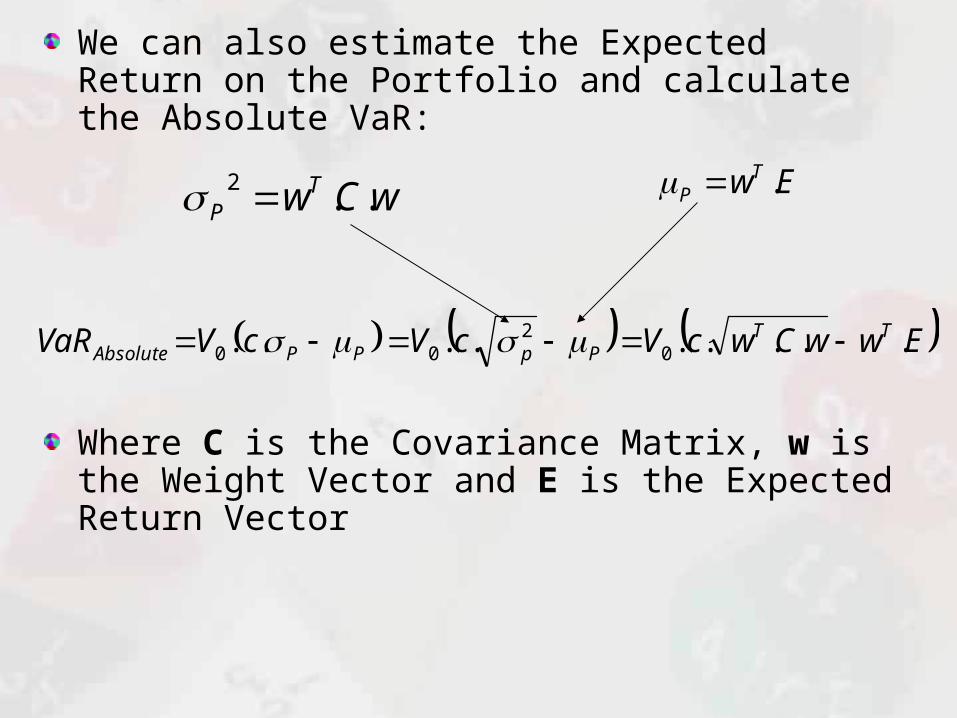
We can also estimate the Expected Return on the Portfolio and calculate the Absolute VaR:
Where C is the Covariance Matrix, w is the Weight Vector and E is the Expected Return Vector
EwwCwcVcVcVVaR TTPpPPAbsolute ......... 0
200
wCwTP ..2 EwT
P .

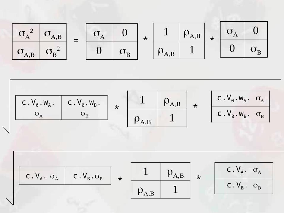
Breaking Down the Calculation
wA wB
wA
wB
* *c.V0 .
c.V0.wA c.V0.wB
c.V0.wA
c.V0.wB
* *
= * *
c.V0.wA. c.V0.wB.
c.V0.wA.
c.V0.wB. * *
c.VA. c.VB.
c.VA.
c.VB. * *
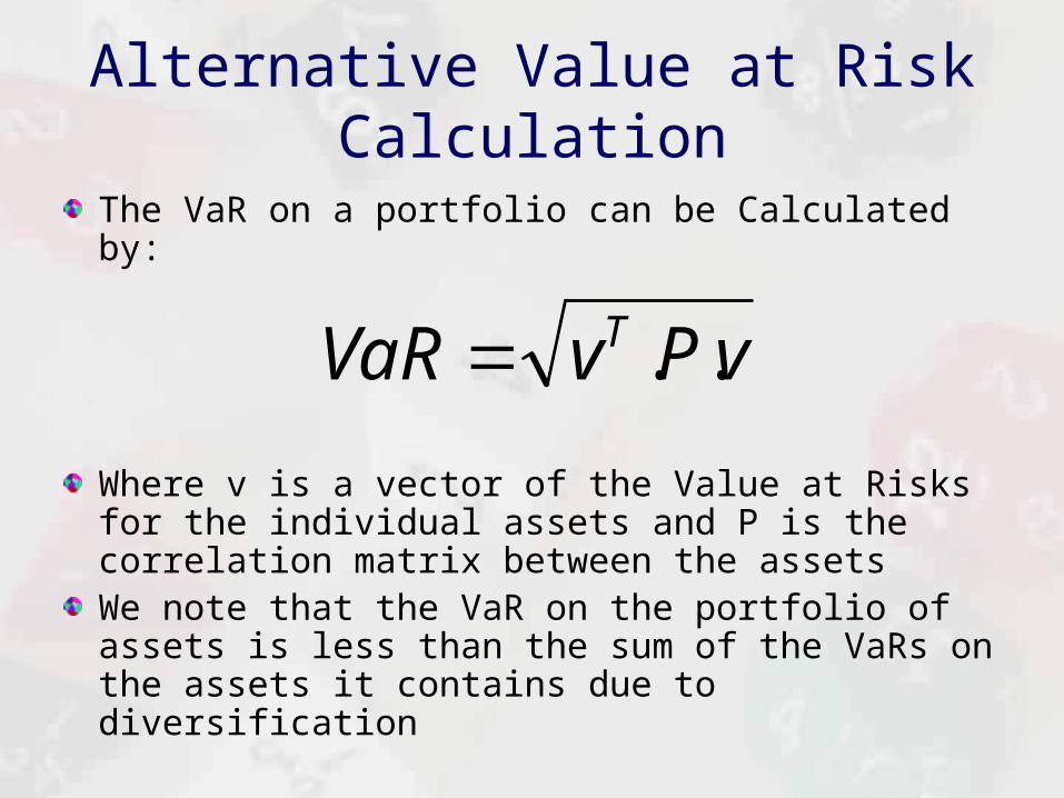
Alternative Value at Risk Calculation
The VaR on a portfolio can be Calculated by:
Where v is a vector of the Value at Risks for the individual assets and P is the correlation matrix between the assetsWe note that the VaR on the portfolio of assets is less than the sum of the VaRs on the assets it contains due to diversification
vPvVaR T ..
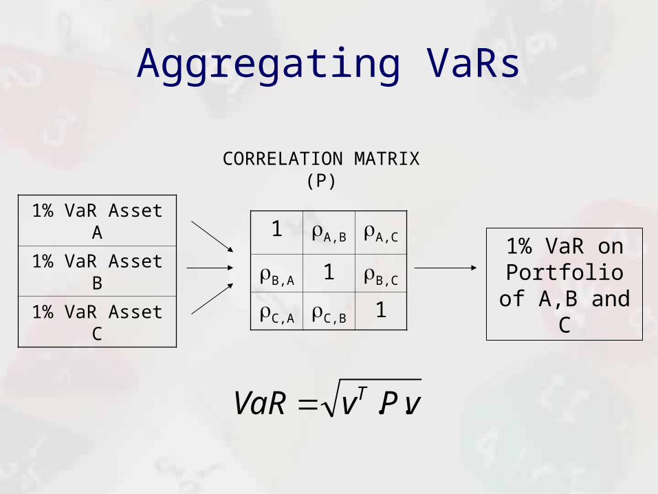
Aggregating VaRs
1 A,B A,C
B,A 1 B,C
C,A C,B 1
vPvVaR T ..
CORRELATION MATRIX(P)
1% VaR on Portfolio of A,B and C
1% VaR Asset A
1% VaR Asset B
1% VaR Asset C
What this Tells Us
What this equation is telling us is that we can derive the Maximum Loss or VaR on a Portfolio of Assets from the Maximum Losses or VaR on the Assets held in the Portfolio
The Maximum Loss or VaR on the Portfolio is less than the sum of the VaR’s on the individual assets because of the Diversification Effect
The extent of this Diversification is determined by the Correlation Matrix

Review QuestionYou are working for a company that has two potential investments A and B. The company estimates that the 0.5% VaR on investment A is £100,000 over the next year (based on a statistical model) and the 0.5% VaR on investment B is £70,000 over the next year (based a 1 in 200 worst case scenario) – the profitability of the two investments are believed to be independent or uncorrelatedThe company says the maximum loss it is willing to take is £130,000 at a 0.5% confidence level, and since these two losses sum to £170,000 the company cannot invest in bothWhy is just adding these losses incorrect and how would you calculate the 0.5% VaR across both investments?

Diversification Effect
170000
-47934.44384
122065.5562
-100000
-50000
0
50000
100000
150000
200000
Undiversified Loss Diversification Effect Diversified Loss

Assumptions: Elliptical DistributionsWe derived our Risk Aggregation Formula using the Normal DistributionThe Risk Aggregation Formula is not restricted to Risks described by the Normal Distribution it apply to any Risk that is Elliptical DistributedThe Elliptical Distributions are a family of distributions (which also include the Multivariate Student and Cauchy Distribution) whose Bivariate Iso-Density Lines form Ellipses or CirclesIn our previous example, if we look at the various independent losses that give an Aggregated VaR of £130,000 they would form an Ellipse or Circle….
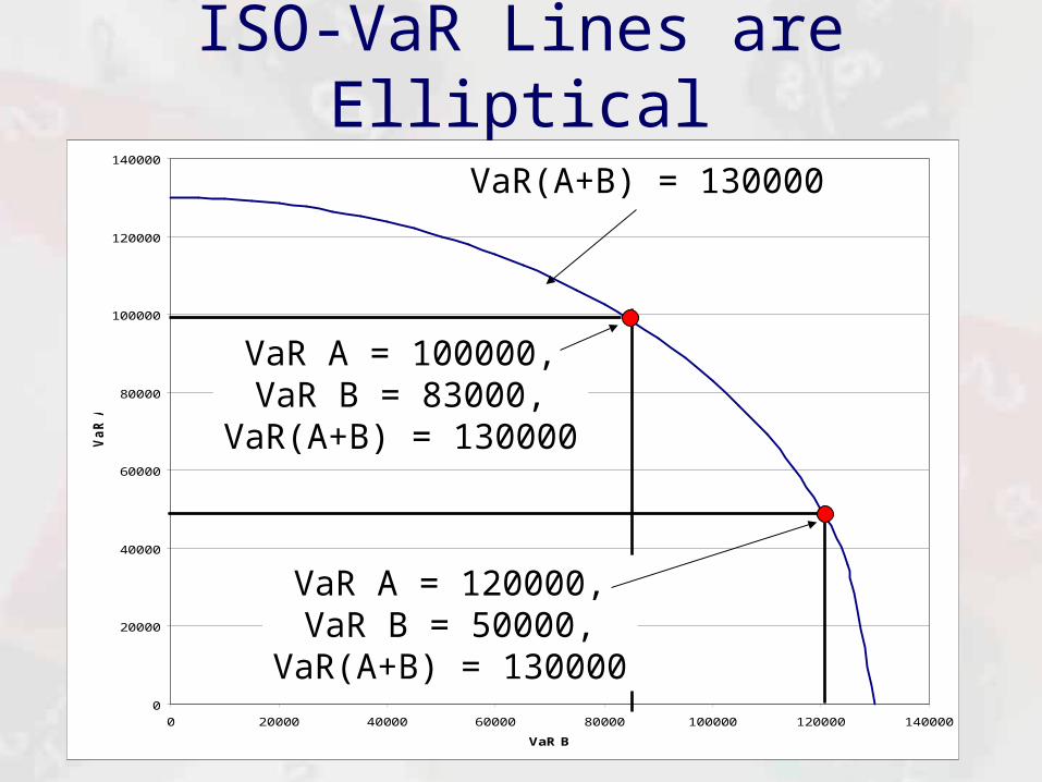
ISO-VaR Lines are Elliptical
0
20000
40000
60000
80000
100000
120000
140000
0 20000 40000 60000 80000 100000 120000 140000
VaR B
Va
R A
VaR(A+B) = 130000
VaR A = 100000,VaR B = 83000,
VaR(A+B) = 130000
VaR A = 120000,VaR B = 50000,
VaR(A+B) = 130000
SCR and Solvency IIInsurance Companies are required by Regulators to hold certainly levels of Capital to protect Policy Holders from the event of the Insurer becoming InsolventIf the insurance company falls below these required levels costly regulatory intervention is enforced and ultimately the company can be declared InsolventIn 2016 the European Union will be introducing a new Unified Risk Based Capital System called Solvency II The Solvency Capital Requirement (SCR) in Solvency II requires Insurance Companies to hold sufficient capital such that Insolvency will only occur once in every 200 years, or that over 1 year they are 99.5% likely to remain SolventFrom the perspective of the Balance Sheet this means that over a one year horizon the probability of Assets being worth less than Liabilities is only 0.5%
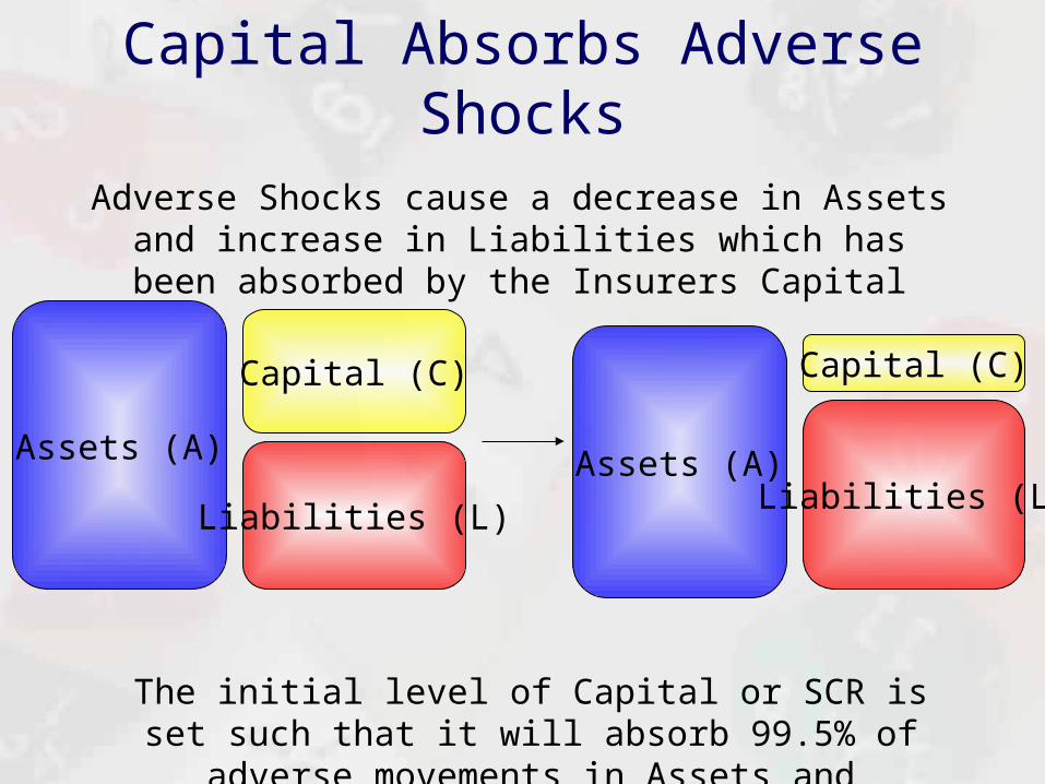
Capital Absorbs Adverse Shocks
Assets (A)
Liabilities (L)
Capital (C)
Assets (A)Liabilities (L)
Capital (C)
The initial level of Capital or SCR is set such that it will absorb 99.5% of adverse movements in Assets and Liabilities
Adverse Shocks cause a decrease in Assets and increase in Liabilities which has been absorbed by the Insurers Capital

Calculating SCR from ScenariosThe Standard Model for Solvency II provides a number of Worse Case Scenarios calibrated to a 1 in 200 year event called ShocksFor documentation of these Shocks see: https://eiopa.europa.eu/Pages/Supervision/Insurance/Solvency-II-Technical-Specifications.aspxFor each Shock the insurance company has to calculate how much capital it would need to absorb either a decrease in Assets or increase in LiabilitiesThe idea behind the SCR is quite simply: if the Insurer has enough capital to absorb this 1 in 200 year shock it will remain Solvent (Assets greater than Liabilities) 99.5% of the time over the next year

Market Risk Shock for Equities in Solvency II
An Insurance Company has £1 million invested in FTSE-100 stocks
In the Technical Specifications for Solvency II the 1 in 200 (PML 99.5%) worst case Scenario or Shock relating to this asset is that equities listed in EEA and OECD countries (Type 2 Equities) will drop by 46.5%
Under this scenario the company would have to have 46.5% of £1 million or £465,000 of Capital to absorb this loss, so the SCR for this risk is £465,000
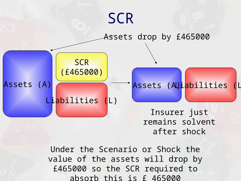
SCR
Assets (A)
Liabilities (L)
SCR(£465000)
Assets (A) Liabilities (L)
Under the Scenario or Shock the value of the assets will drop by £465000 so the SCR required to absorb
this is £ 465000
Assets drop by £465000
Insurer just remains solvent after shock
Market Risk for Equities Type 2
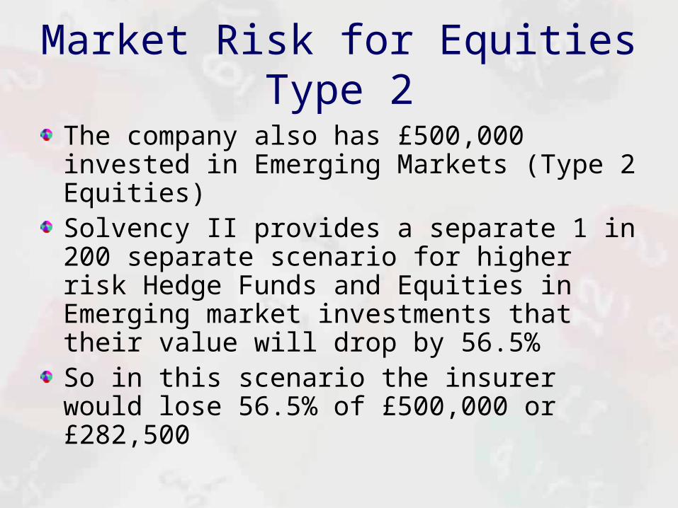
The company also has £500,000 invested in Emerging Markets (Type 2 Equities)Solvency II provides a separate 1 in 200 separate scenario for higher risk Hedge Funds and Equities in Emerging market investments that their value will drop by 56.5%So in this scenario the insurer would lose 56.5% of £500,000 or £282,500

Combining the Two Scenarios
We could simply add these two SCRs together to get the SCR required to absorb both these scenarios: £465,000 + £282,500 = £747,500As we saw adding scenarios in this way assumes they are perfectly correlatedThe Solvency II system provides a correlation matrix set by the Regulator that Insurance Company is expected to use to combine the SCRs

Equity Market Risk Correlation Matrix equity
1 0.75
0.75 1
(Type 1)EEA and OECD
Equities
(Type 2)Emerging Markets,
Hedge Funds
(Type 1) (Type 2)
Solvency II Risk Aggregation Formula
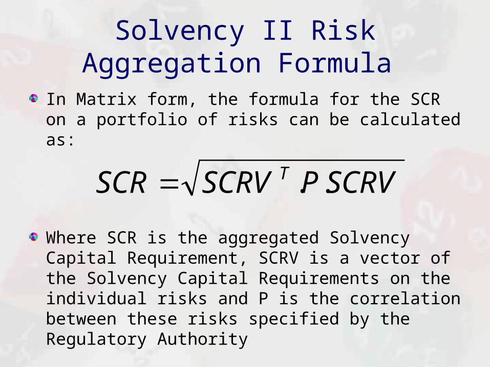
In Matrix form, the formula for the SCR on a portfolio of risks can be calculated as:
Where SCR is the aggregated Solvency Capital Requirement, SCRV is a vector of the Solvency Capital Requirements on the individual risks and P is the correlation between these risks specified by the Regulatory Authority
SCRVPSCRVSCR T ..
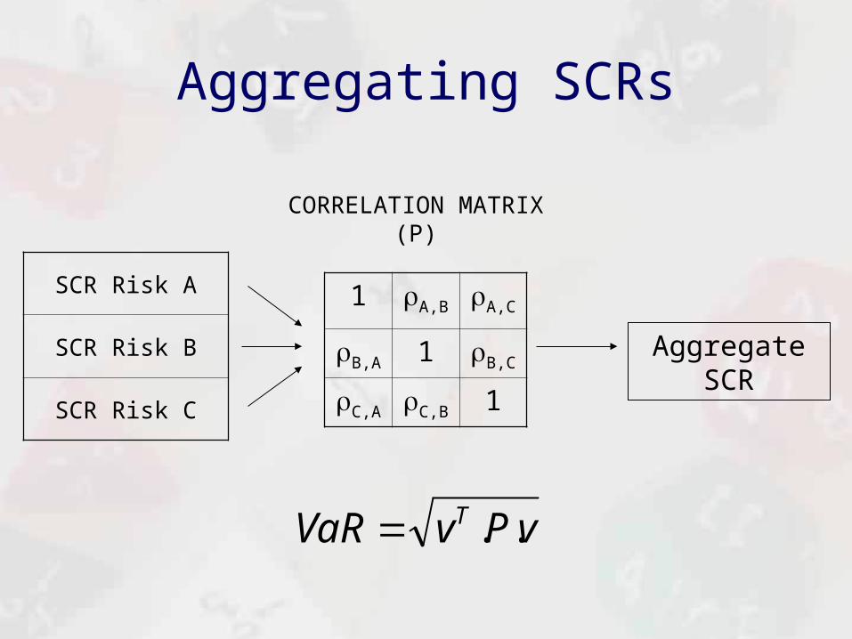
Aggregating SCRs
1 A,B A,C
B,A 1 B,C
C,A C,B 1
vPvVaR T ..
CORRELATION MATRIX(P)
Aggregate SCR
SCR Risk A
SCR Risk B
SCR Risk C

SCR Aggregation
465,000
282,500
SCRVequity=
SQRT(MMULT(MMULT(TRANSPOSE(E5:E6),H5:I6),E5:E6)) = 702192
SCRVPSCRVSCR T ..

SCR Diversification Effect
-£45307.00659
£702192£747500
-100000
0
100000
200000
300000
400000
500000
600000
700000
800000
UnDiversified SCR Diversification Effect Diversified SCR

Optimization Problems Within Solvency II
The Standard Model in Solvency II is basically an application of the Mean-Variance Model and it introduces the idea of “Efficient Combinations” of Assets and LiabilitiesFor example, in our previous example let us say the company expects a 5% return on its Investments in the FTSE and a 7% return on its Emerging Market Investments.Initially the Expected Profit on the investments is £85000 and the SCR is £702193Can we find the combination of assets that will maintain our profitability but minimize our SCR?

Shocks for Other Types of Market Risks
We just calculated the SCR for the Equity Component of the Market Risk Module
The Market Risk Module in Solvency II provides Shocks for movements in Interest Rates (1 Year Interest Rates rise by 70%), the value of Property Investments (drop by 25%), the value of Currencies (rise or fall by 25%) and so on
The Insurance Company could go away and calculate the SCR required to absorb these shocks and put them into a Vector…
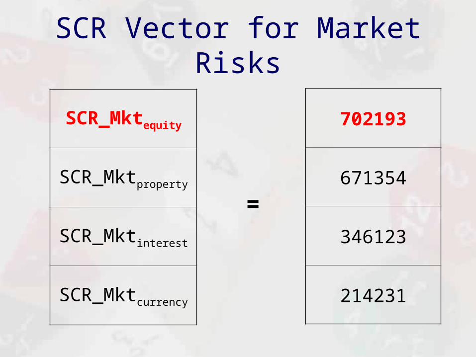
SCR Vector for Market Risks
SCR_Mktequity
SCR_Mktproperty
SCR_Mktinterest
SCR_Mktcurrency
702193
671354
346123
214231
=
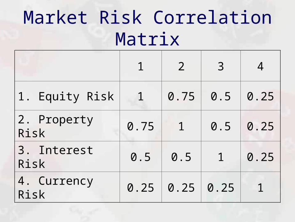
Market Risk Correlation Matrix
1 2 3 4
1. Equity Risk 1 0.75 0.5 0.25
2. Property Risk 0.75 1 0.5 0.25
3. Interest Risk 0.5 0.5 1 0.25
4. Currency Risk 0.25 0.25 0.25 1

Solvency II Modules Overview
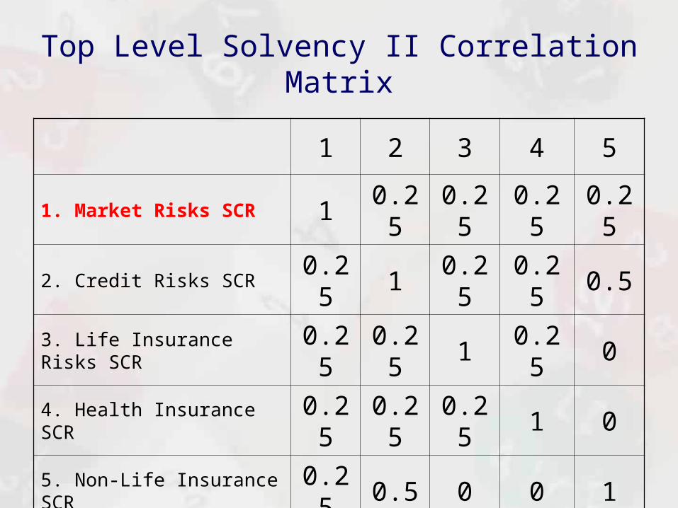
Top Level Solvency II Correlation Matrix
1 2 3 4 5
1. Market Risks SCR 1 0.25 0.25 0.25 0.25
2. Credit Risks SCR 0.25 1 0.25 0.25 0.5
3. Life Insurance Risks SCR 0.25 0.25 1 0.25 0
4. Health Insurance SCR 0.25 0.25 0.25 1 0
5. Non-Life Insurance SCR 0.25 0.5 0 0 1
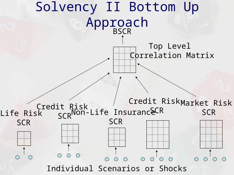
Solvency II Bottom Up Approach
Market Risk SCR
BSCR
Credit Risk SCRLife Risk
SCR
Credit Risk SCR Non-Life Insurance
SCR
Top Level Correlation Matrix
Individual Scenarios or Shocks

Premium Risk in Solvency IIWe looked at the Frequency Severity Model and how it could be used to model the risk that premiums are less than claims (Premium Risk or Underwriting Risk)In the Standard Model in Solvency II the 1 in 200 shock resulting in a loss due to claims being higher than premiums is approximately calculated using the formula**:
Where NP is the Net Premium and is a risk factor selected based on the Line of Business (the more riskier the line the higher the risk factor)The risk factor is essentially the industry average standard deviation of the Net Claims Ratio for a particular Line of Business
NPSCR ..3

Some Risk Factors for Different Classes
Line of Business Risk Factor
Motor Liability 9.5%
Other Motor 10%
MAT (Marine Aviation) 17%
Fire 10%
Liability 15%

Log Normal Distribution for the Net Claims Ratio (Net Claims / Net Premiums) for MAT: = 100% = 17%
0
0.5
1
1.5
2
2.5
40.00% 80.00% 120.00% 160.00%
%17*3%100%152
)2^17.0,1,995.0(
CDFLogNormalI
0.5% tail
When the Net Claims Ratio is 152%, Net Claims are 152% of Net Premiums and the Underwriting Loss (NP – NC) is 52% * NP or Approximately 3 * 17% * NP

Correlation Matrix by LOB
1 2 3 4 5
1. Motor Liability 1.0 0.5 0.5 0.25 0.5
2. Other Motor 0.5 1.0 0.25 0.25 0.25
3. MAT 0.5 0.25 1.0 0.25 0.25
4. Fire 0.25 0.25 0.25 1.0 0.25
5. Liability 0.5 0.25 0.25 0.25 1.0
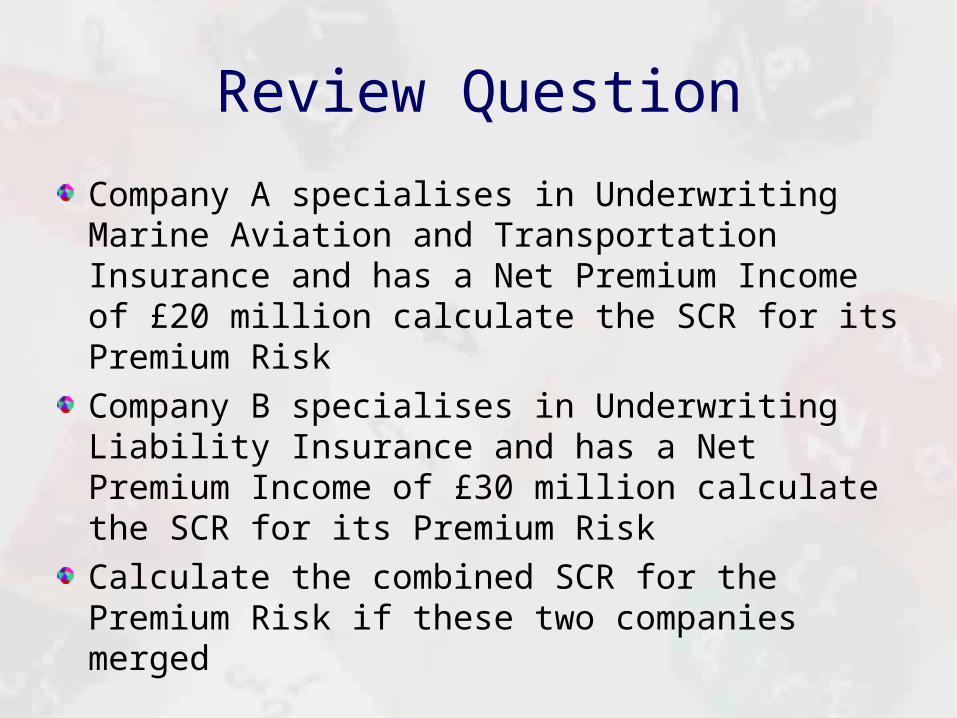
Review Question
Company A specialises in Underwriting Marine Aviation and Transportation Insurance and has a Net Premium Income of £20 million calculate the SCR for its Premium Risk
Company B specialises in Underwriting Liability Insurance and has a Net Premium Income of £30 million calculate the SCR for its Premium Risk
Calculate the combined SCR for the Premium Risk if these two companies merged
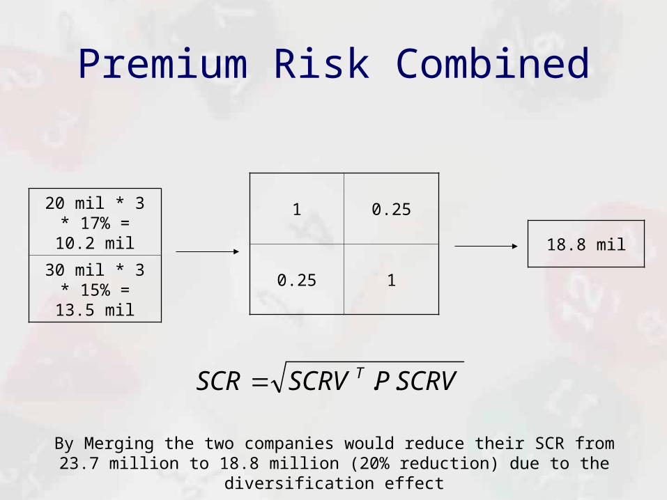
Premium Risk Combined
20 mil * 3 * 17% = 10.2 mil
30 mil * 3 * 15% = 13.5 mil
1 0.25
0.25 1
SCRVPSCRVSCR T ..
18.8 mil
By Merging the two companies would reduce their SCR from 23.7 million to 18.8 million (20% reduction) due to the diversification effect
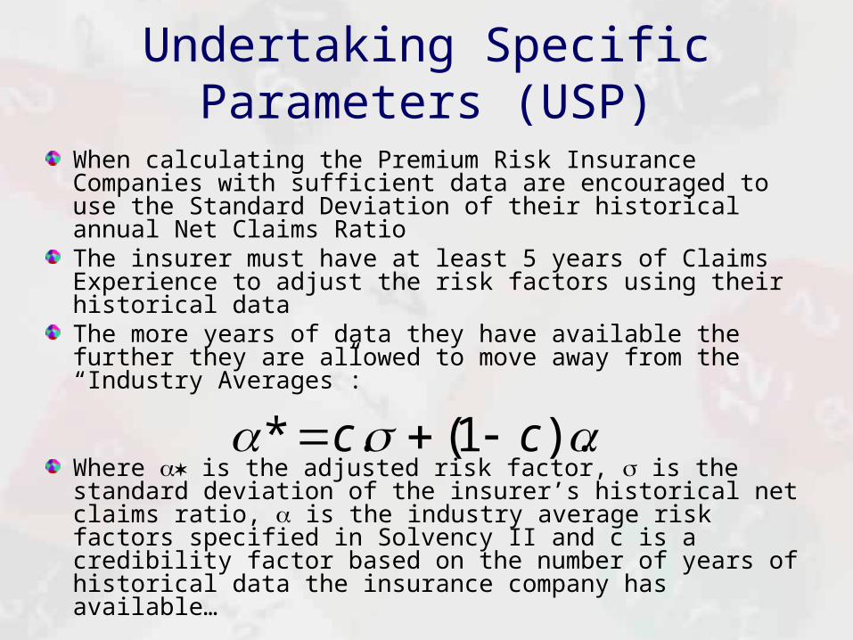
Undertaking Specific Parameters (USP)
When calculating the Premium Risk Insurance Companies with sufficient data are encouraged to use the Standard Deviation of their historical annual Net Claims RatioThe insurer must have at least 5 years of Claims Experience to adjust the risk factors using their historical dataThe more years of data they have available the further they are allowed to move away from the “Industry Averages”:
Where is the adjusted risk factor, is the standard deviation of the insurer’s historical net claims ratio, is the industry average risk factors specified in Solvency II and c is a credibility factor based on the number of years of historical data the insurance company has available…
).1(.* cc

Credibility Factors for Years of Data for Liability Insurance
5 6 7 8 9 10 11 12 13 14 >=15
34% 43% 51% 59% 67% 74% 81% 87% 92% 96% 100%
Years of Data
Credibility (c)
For example, the insurance company calculates the Standard Deviation of its Net Claims Ratio on its Liability Insurance Portfolio over the last 10 years was 12% its adjusted risk factor would be:
What would the adjusted risk factor have been if the standard deviation was still 12% and based on 15 years of data?
%78.12%15*)74.01(%12*74.0*
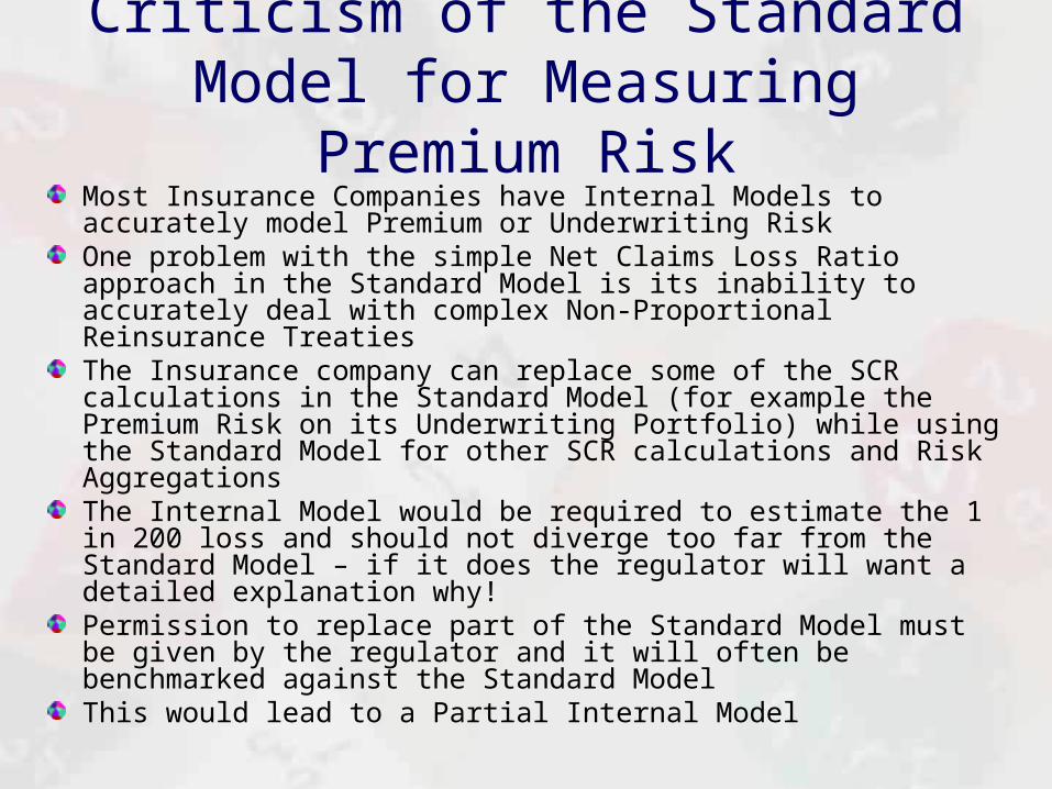
Criticism of the Standard Model for Measuring Premium Risk
Most Insurance Companies have Internal Models to accurately model Premium or Underwriting RiskOne problem with the simple Net Claims Loss Ratio approach in the Standard Model is its inability to accurately deal with complex Non-Proportional Reinsurance TreatiesThe Insurance company can replace some of the SCR calculations in the Standard Model (for example the Premium Risk on its Underwriting Portfolio) while using the Standard Model for other SCR calculations and Risk AggregationsThe Internal Model would be required to estimate the 1 in 200 loss and should not diverge too far from the Standard Model – if it does the regulator will want a detailed explanation why!Permission to replace part of the Standard Model must be given by the regulator and it will often be benchmarked against the Standard ModelThis would lead to a Partial Internal Model
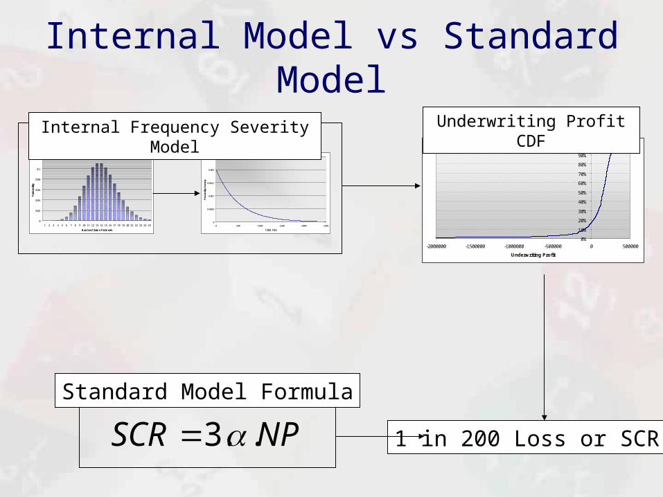
Internal Model vs Standard Model
0
0.02
0.04
0.06
0.08
0.1
0.12
1 2 3 4 5 6 7 8 9 10 11 12 13 14 15 16 17 18 19 20 21 22 23 24 25
Number Claims Per Week
Pro
bab
ility
0
0.0005
0.001
0.0015
0.002
0.0025
0 500 1000 1500 2000 2500
Claim Size
Pro
bab
ility
Den
isty
NPSCR ..3
Internal Frequency Severity Model
Standard Model Formula
1 in 200 Loss or SCR
0%
10%
20%
30%
40%
50%
60%
70%
80%
90%
100%
-2000000 -1500000 -1000000 -500000 0 500000
Underwriting Profit
Underwriting Profit CDF

Full Internal ModelMany of the Largest Insurance and Reinsurance Companies have spent millions of pounds replacing the Standard Model with their own Full Internal Models – mainly based on Monte Carlo SimulationsIn addition to replacing the individual SCR calculations these Internal Models replace the Correlation Matrix Aggregation Formula with more flexible CopulaCopula are an extremely flexible way to describe the interdependence between Risks and we will look at their use in Credit Risk ModelsFull Internal Models will be heavily scrutinised by regulators if their results diverge too widely from the Standard Model
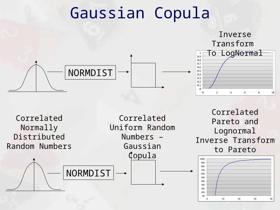
Gaussian Copula
Correlated Normally Distributed Random
Numbers
NORMDIST
NORMDIST
Correlated Uniform Random Numbers –
Gaussian Copula
0
0.1
0.20.3
0.4
0.5
0.6
0.70.8
0.9
1
0 2 4 6 8 10
0%
10%
20%
30%
40%
50%
60%
70%
80%
90%
100%
0 10 20 30 40
Inverse Transform To LogNormal
Inverse Transform to Pareto
Correlated Pareto and Lognormal
Appendix: Diversified & Undiversified VaR
In the event of a crash all assets tend to move down together – ie high correlationWhen this occurs the effects of diversification are negated and the volatility of the portfolio is greaterFor this reason it is suggested that when calculating the variance on a portfolio for a VaR calculation (worst case scenario) it should incorporate high positive correlations, not day-to-day correlations
In the extreme case this can be achieved by setting the correlation terms in the correlations between assets to 1 (perfect positive correlation)
The effects of this will be to increase the variance of the portfolio and thus increase the maximum loss by removing the effect of diversification from the portfolio
When we calculate VaR on this basis we are calculating Undiversified VaR
If we use normal day-to-day correlations we calculate Diversified VaR
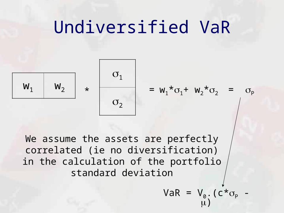
Undiversified VaR
w1 w2
1
2
* = w1*1+ w2*2 = P
VaR = V0.(c*P - )
We assume the assets are perfectly correlated (ie no diversification) in the calculation of the portfolio
standard deviation
Appendix: The Log-Normal Distribution
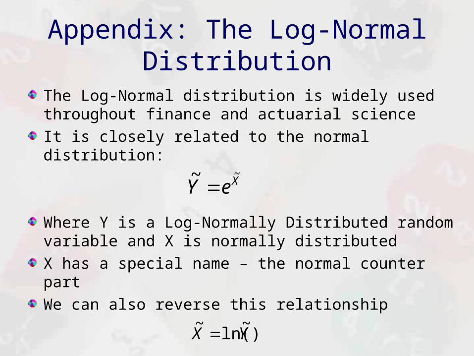
The Log-Normal distribution is widely used throughout finance and actuarial science
It is closely related to the normal distribution:
Where Y is a Log-Normally Distributed random variable and X is normally distributed
X has a special name – the normal counter part
We can also reverse this relationship
XeY~~
)~
ln(~
YX
Important Result!
0
0.1
0.2
0.3
0.4
0.5
0.6
-1 1 3 5 7 9 11
0~r
0
0.05
0.1
0.15
0.2
0.25
0.3
0.35
0.4
0.45
0.5
-3 -2 -1 0 1 2 3
Pro
ba
bil
ity
De
ns
ity
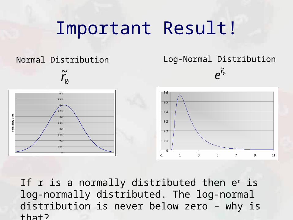
If r is a normally distributed then er is log-normally distributed. The log-normal distribution is never below zero – why is that?
0~re
Normal Distribution Log-Normal Distribution

Log-Normal Excel Formula
The PDF of a log-normally distributed at a value Y is:
=NORMDIST(LN(Y),,,FALSE)
Where is the mean of the normal counterpart and is the standard deviation (Note this uses the density for the normal distribution)
The CDF for a log-normally distributed random variable is:
=NORMDIST(LN(Y),,,TRUE)

The inverse CDF for a log-normally distributed random variable is
=EXP(NORMINV(P,,))
Where P is the probability of the log-normally distributed random variable being less than or equal to some level
Notice that we are doing here is finding the quantile of the normal counterpart and then implying the quantile of the log-normal from this
Fitting the Log-Normal
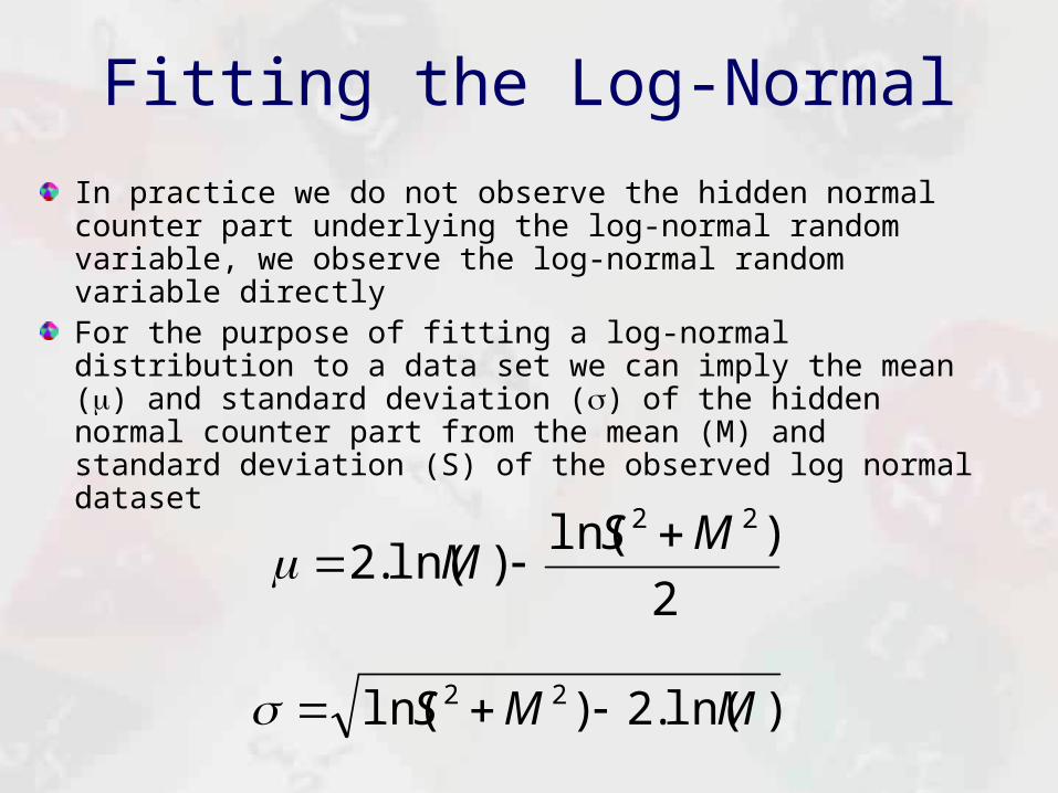
In practice we do not observe the hidden normal counter part underlying the log-normal random variable, we observe the log-normal random variable directlyFor the purpose of fitting a log-normal distribution to a data set we can imply the mean () and standard deviation () of the hidden normal counter part from the mean (M) and standard deviation (S) of the observed log normal dataset
2
)ln()ln(.2
22 MSM
)ln(.2)ln( 22 MMS

Log Normal VBA Functions
Public Function LogNormalCDF(X, Average, Variance)SCM = Variance + (Average ^ 2)mu = 2 * Log(Average) - 0.5 * Log(SCM)s = (Log(SCM) - 2 * Log(Average)) ^ 0.5LogNormalCDF = Application.WorksheetFunction.NormDist(Log(X), mu, s, True)End Function
Public Function LogNormalInverseCDF(P, Average, Variance)SCM = Variance + (Average ^ 2)mu = 2 * Log(Average) - 0.5 * Log(SCM)s = (Log(SCM) - 2 * Log(Average)) ^ 0.5LogNormalInverseCDF = Exp(Application.WorksheetFunction.NormInv(P, mu, s))End Function
Product Limit TheoryLike the Normal Distribution, the Log-Normal distribution also occurs in the world about us
The explanation behind why we see the Log-Normal distribution is the Product Limit Theory
The Product Limit theory states that if we multiply any number of independent positive random variables we can expect their product to be Log-Normally Distributed
Anything that grows by random proportional amounts over time should be log-normally distributed
An example of something that grows randomly in this way over time is the value of assets….

Random Compounding Over Time
)~1.(12 rVV 0V
1~r
)~1.(01 rVV 2
~r 2~r
0
0.05
0.1
0.15
0.2
0.25
0.3
0.35
0.4
0.45
0.5
-3 -2 -1 0 1 2 3
Pro
ba
bil
ity
De
ns
ity
0
0.05
0.1
0.15
0.2
0.25
0.3
0.35
0.4
0.45
0.5
-3 -2 -1 0 1 2 3
Pro
ba
bil
ity
De
ns
ity
0
0.05
0.1
0.15
0.2
0.25
0.3
0.35
0.4
0.45
0.5
-3 -2 -1 0 1 2 3
Pro
ba
bil
ity
De
ns
ity

Our Experiment
* * * *
!0
0.1
0.2
0.3
0.4
0.5
0.6
-1 1 3 5 7 9 11
0
0.05
0.1
0.15
0.2
0.25
0.3
0.35
0.4
0.45
0.5
-3 -2 -1 0 1 2 3
Pro
ba
bil
ity
De
ns
ity
0
0.05
0.1
0.15
0.2
0.25
0.3
0.35
0.4
0.45
0.5
-3 -2 -1 0 1 2 3
Pro
ba
bil
ity
De
ns
ity
0
0.05
0.1
0.15
0.2
0.25
0.3
0.35
0.4
0.45
0.5
-3 -2 -1 0 1 2 3
Pro
ba
bil
ity
De
ns
ity
0
0.05
0.1
0.15
0.2
0.25
0.3
0.35
0.4
0.45
0.5
-3 -2 -1 0 1 2 3
Pro
ba
bil
ity
De
ns
ity
0
0.05
0.1
0.15
0.2
0.25
0.3
0.35
0.4
0.45
0.5
-3 -2 -1 0 1 2 3
Pro
ba
bil
ity
De
ns
ity

Shifted Log-Normal and Actuarial Science
Actuarial Science makes wide use of a slightly different form of the Log-Normal:
Where C is the shift factor which is to be determined in addition to the mean and standard deviation of the normal counter part xThe shifted log normal is sometimes used to model claim severities but is also widely used to Model the distribution of Aggregate Claims (the Solvency II standard model currently uses a Log Normal for this)
CeY X ~~
Fitting the Shifted Log Normal with Skew
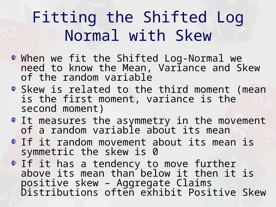
When we fit the Shifted Log-Normal we need to know the Mean, Variance and Skew of the random variableSkew is related to the third moment (mean is the first moment, variance is the second moment)It measures the asymmetry in the movement of a random variable about its meanIf it random movement about its mean is symmetric the skew is 0If it has a tendency to move further above its mean than below it then it is positive skew – Aggregate Claims Distributions often exhibit Positive Skew

The third moment is the average of the cubed difference of the random variable from its mean:
Skew the third moment normalised by the standard deviation:
In Excel this can be calculated using the SKEW function
By fitting the Mean, Variance and Skew of the Aggregate Claims distribution we can obtain a much better fit than with just the Mean and Variance
The Skew like the Mean and Variance of the Aggregate Claims Distribution can often be derived analytically…
3
3
1 xn
33

Appendix: Third Moment of the Compound Poisson
In a previous class saw that the first two moments of the compound Poisson Process could be calculated by
The third moment is
Where is the average frequency of claims, C is the average claim severity,
C is the variance of claim severity and 3C is the third moment of claim severity
CSE .)(
22 ..)( CCSVar
3233 ....3.)( CCCCS

Appendix: Fitting Shifted Log Normal
The first step in fitting the shifted log normal is to find the root of (where is a positive skew coefficient):
Using this root we can find the following:
0.33
S
MC )1ln( 22
2)ln(
2 CM

Appendix: Risk Over Time
Let us say we assume that continuously compounded returns are described by a normal distributionThe relationship between the portfolio value today v0 and the value tomorrow v1, where r0 is today’s random proportional change
0~
01 .~ revv • r0 is normally distributed by assumption
• v1 is log normally distributed since er0 is log-normally distributed
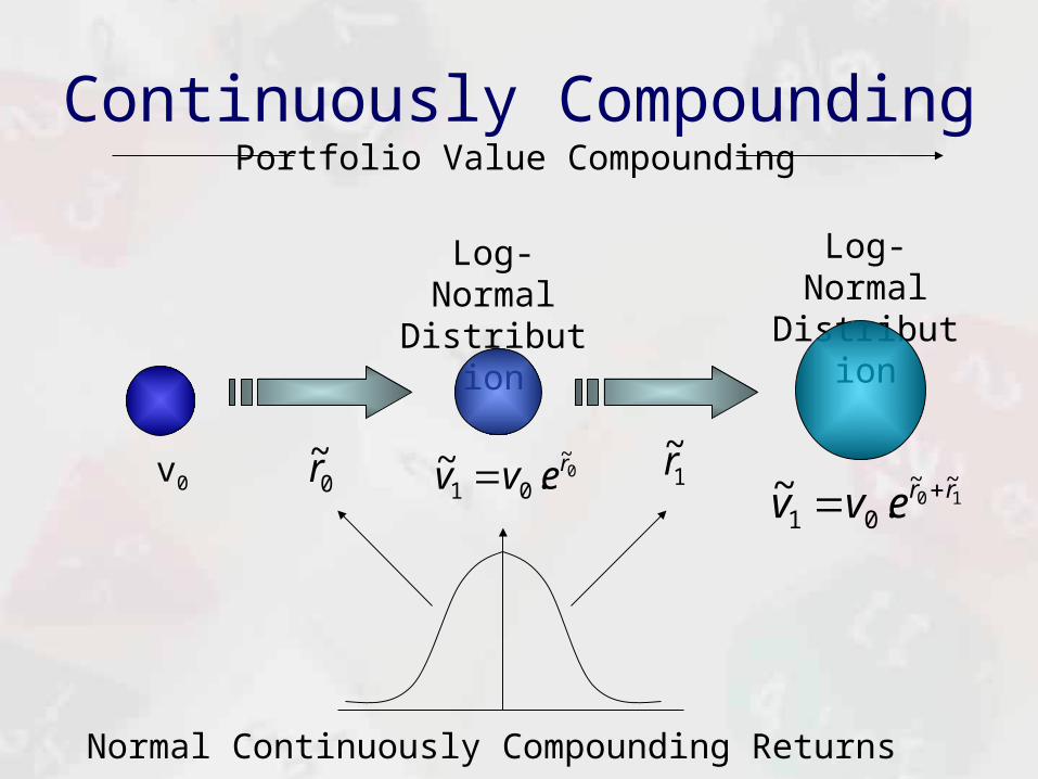
Continuously Compounding
0~
01 .~ revv v0
Log-Normal Distribution
Log-Normal Distribution
0~r 1
~r
Normal Continuously Compounding Returns
Portfolio Value Compounding
10~~
01 .~ rrevv

Now the relationship between v0 and v2
1~
12 .~~ revv 1010~~
0
~~
0
~
02 ....~ rrrrR eveevevv • R is equal to r0 + r1 so it is normally distributed
• v2 is log-normal since er0+r1 is log-normally distributed
• Let us say that r0 and r1 are both sampled from the same normal distribution with a given mean and standard deviation • Then the mean of R is 2. ( + ) and the variance is 2.2 (2 + 2)
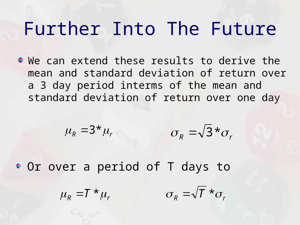
Further Into The Future
We can extend these results to derive the mean and standard deviation of return over a 3 day period interms of the mean and standard deviation of return over one day
rR *3rR *3
Or over a period of T days to
rR T * rR T *
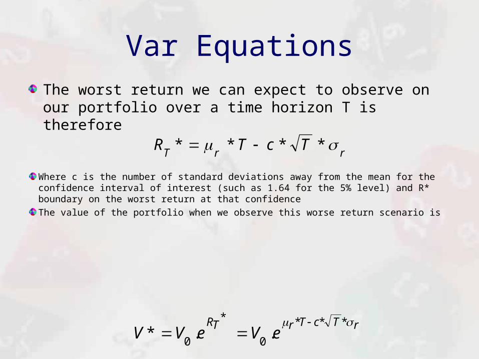
Var Equations
The worst return we can expect to observe on our portfolio over a time horizon T is therefore
rrTTcTR ****
Where c is the number of standard deviations away from the mean for the confidence interval of interest (such as 1.64 for the 5% level) and R* boundary on the worst return at that confidence
The value of the portfolio when we observe this worse return scenario is
rTcTrTReVeVV
***
0
*
0..*