risk assessment - who.int · characterisation. the task of risk management is one of deciding the...

© 2001 World Health Organization (WHO). Water Quality: Guidelines, Standards and Health. Edited byLorna Fewtrell and Jamie Bartram. Published by IWA Publishing, London, UK. ISBN: 1 900222 28 0

8Risk assessment

Chuck Haas and Joseph N.S. Eisenberg

This chapter introduces the technique of microbial risk assessment and outlinesits development from a simple approach based upon a chemical risk model to anepidemiologically-based model that accounts for, among other things,secondary transmission and protective immunity. Two case studies arepresented to highlight the different approaches.

8.1 BACKGROUNDQuantifiable risk assessment was initially developed, largely, to assess humanhealth risks associated with exposure to chemicals (NAS 1983) and, in itssimplest form, consists of four steps, namely:

hazard assessmentexposure assessmentdose–response analysisrisk characterisation.

162 Water Quality: Guidelines, Standards and Health

The output from these steps feeds into a risk management process. As will beseen in later sections this basic model (often referred to as the chemical riskparadigm) has been extended to account for the dynamic and epidemiologiccharacteristics of infectious disease processes. The following sub-sectionselaborate on the chemical risk paradigm as outlined above.

8.2 CHEMICAL RISK PARADIGM

8.2.1 Hazard assessmentFor micro-organisms, hazard assessment (i.e. the identification of a pathogen asan agent of potential significance) is generally a straightforward task. The majortasks of Quantitative Microbiological Risk Assessment (QMRA) are, therefore,focused on exposure assessment, dose–response analysis and riskcharacterisation. The task of risk management is one of deciding the necessityof any action based upon the risk characterisation outputs, and incorporatessignificant policy and trans-scientific concerns.

One outcome of the hazard analysis is a decision as to the principalconsequence(s) to be quantified in the formal risk assessment. With micro-organisms, consequences may include infection (without apparent illness),morbidity or mortality; furthermore, these events may occur in the generalpopulation, or at higher frequency in susceptible sub-populations. Althoughmortality from infectious agents, even in the general population, cannot beregarded as negligible (Haas et al. 1993), the general tendency (in watermicrobiology) has been to regard infection in the general population as theparticular hazard for which protection is required. This has been justified basedon a balance between the degree of conservatism inherent in using infection asan endpoint and the (current) inability to quantify the risks to more susceptiblesub-populations (Macler and Regli 1993).

8.2.2 Exposure assessmentThe purpose of an exposure assessment is to determine the microbial dosestypically consumed by the direct user of a water (or food). In the case of watermicrobiology, this may necessitate the estimation of raw water micro-organismlevels followed by estimation of the likely changes in microbial concentrationswith treatment, storage and distribution to the end-user (Regli et al. 1991; Roseet al. 1991). A second issue arising in exposure assessment is the amount ofingested material per ‘exposure’. As a default number, two litres/person-day isused to estimate drinking water exposure (Macler and Regli 1993), although thismay be conservative (Roseberry and Burmaster 1992). For contact recreational

Risk assessment 163

exposure, 100 ml/day has often been assumed as an exposure measure (Haas1983a), but actual data to validate this number are lacking.

8.2.3 Dose–response analysisIt is generally necessary to fit a parametric dose–response relationship toexperimental data since the desired risk (and dose) which will serve to protectpublic health is often far lower than can be directly measured in experimentalsubjects (at practical numbers of subjects). Hence it is necessary to extrapolate afitted dose–response curve into the low-dose region.

In QMRA, for many micro-organisms, human dose–response studies areavailable which can be used to estimate the effects of low level exposure tomicro-organisms. In prior work, it has been found that these studies may beadequately described by one of two semi-mechanistic models of the infectionprocess. In the exponential model, which may be derived from the assumptionof random occurrence of micro-organisms along with a constant probability ofinitiation of infection by a single organism (r), the probability of infection (PI) isgiven as a function of the ingested dose (d) by:

(8.1)

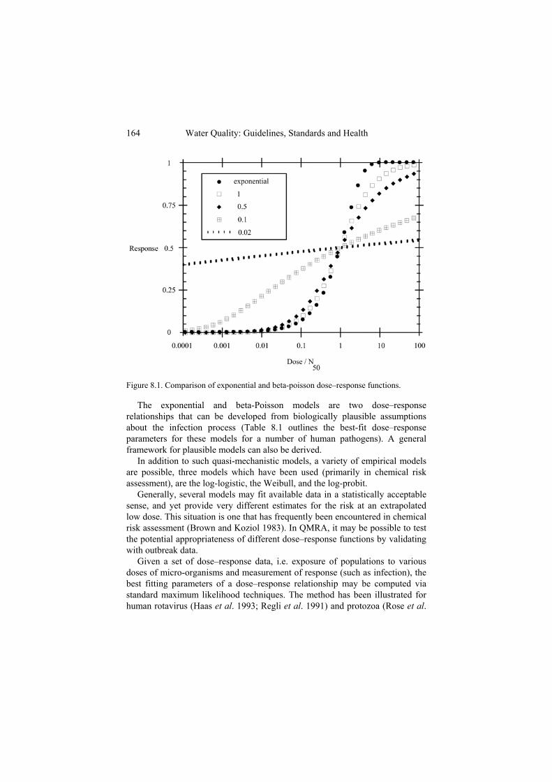
For many micro-organisms, the dose–response relationship is shallower thanreflected by Equation 8.1, suggesting some degree of heterogeneity in themicro-organism-host interaction. This can be successfully described by the beta-Poisson model, which can be developed from Equation 8.1 if the infectionprobability is itself distributed according to a beta distribution (Furumoto andMickey 1967a,b; Haas 1983b). This model is described by two parameters, amedian infectious dose (N50) and a slope parameter ( ):

(8.2)

Figure 8.1 depicts the effect of the slope parameter on the dose–responserelationship; in the limit of , Equation 8.2 approaches Equation 8.1.

)exp(1 rdPI


Figure 8.1. Comparison of exponential and beta-poisson dose–response functions.

The exponential and beta-Poisson models are two dose–responserelationships that can be developed from biologically plausible assumptionsabout the infection process (Table 8.1 outlines the best-fit dose–responseparameters for these models for a number of human pathogens). A generalframework for plausible models can also be derived.

In addition to such quasi-mechanistic models, a variety of empirical modelsare possible, three models which have been used (primarily in chemical riskassessment), are the log-logistic, the Weibull, and the log-probit.

Generally, several models may fit available data in a statistically acceptablesense, and yet provide very different estimates for the risk at an extrapolatedlow dose. This situation is one that has frequently been encountered in chemicalrisk assessment (Brown and Koziol 1983). In QMRA, it may be possible to testthe potential appropriateness of different dose–response functions by validatingwith outbreak data.

Given a set of dose–response data, i.e. exposure of populations to variousdoses of micro-organisms and measurement of response (such as infection), thebest fitting parameters of a dose–response relationship may be computed viastandard maximum likelihood techniques. The method has been illustrated forhuman rotavirus (Haas et al. 1993; Regli et al. 1991) and protozoa (Rose et al.

Risk assessment 165

1991). Confidence limits to the parameters can then be found, and used as abasis for low-dose extrapolation. It should be noted, however, that in generaldose–response studies have been conducted on healthy adults and may not,therefore, reflect the response of the general population.

Table 8.1. Table of best-fit dose–response parameters (human)

Organism Exponential Beta Poisson Referencek N50

Poliovirus I (Minor) 109.87 Minor et al, 1981Rotavirus 6.17 0.2531 Haas et al. 1993;

Ward et al. 1986Hepatitis A virus(a) 1.8229 Ward et al. 1958Adenovirus 4 2.397 Couch et al. 1966Echovirus 12 78.3 Akin 1981Coxsackie(b) 69.1 Couch et al. 1965;

Suptel, 1963Salmonella(c) 23,600 0.3126 Haas et al. 1999Salmonella typhosa 3.60 × 106 0.1086 Hornick et al. 1966Shigella(d) 1120 0.2100 Haas et al. 1999Escherichia coli(e) 8.60 × 107 0.1778 Haas et al. 1999Campylobacter jejuni 896 0.145 Medema et al. 1996Vibrio cholera 243 0.25 Haas et al. 1999Entamoeba coli 341 0.1008 Rendtorff 1954Cryptosporidium parvum 238 Haas et al. 1996;

Dupont et al. 1995Giardia lamblia 50.23 Rose et al. 1991

(a) dose in grams of faeces (of excreting infected individuals)(b) B4 and A21 strains pooled(c) multiple (non-typhoid) pathogenic strains (S. pullorum excluded)(d) flexnerii and dysenteriae pooled(e) Nonenterohaemorrhagic strains (except O111)

8.2.4 Risk characterisationThe process of risk characterisation combines the information on exposure anddose–response into an overall estimation of likelihood of an adverseconsequence. This may be done in two basic ways. First, a single point estimateof exposure (i.e. number of organisms ingested) can be combined with a singlepoint estimate of the dose–response parameters to compute a point estimate ofrisk. This may be done using a ‘best’ estimate, designed to obtain a measure ofcentral tendency, or using an extreme estimate, designed to obtain a measure ofconsequence in some more adversely affected circumstance. An alternativeapproach, which is currently receiving increasing favour, is to characterise the


full distribution of exposure and dose–response relationships, and to combinethese using various tools (for example, Monte Carlo analysis) into a distributionof risk. This approach conveys important information on the relativeimprecision of the risk estimate, as well as measures of central tendency andextreme values (Burmaster and Anderson 1994; Finkel 1990).

One important outcome of the risk characterisation process using a MonteCarlo approach is the assessment of the relative contribution of uncertaintyand variability to a risk estimate. Variability may be defined as the intrinsicheterogeneity that leads to differential risk among sectors of the exposedgroup, perhaps resulting from differential sensitivities or differentialexposures. Uncertainty may be defined as the factors of imprecision andinaccuracy that limit the ability to exactly quantify risk. Uncertainty may bereduced by additional resources, for example devoted to characterisation ofthe dose–response relationship. Variability represents a lower limit to theoverall risk distribution.

Two aspects of risk characterisation deserve further comment. In general, allavailable dose–response information for micro-organisms (human or animal)pertains to response to single (bolus) doses. In actual environmental (or food)exposures, doses may occur over time (or may even be relatively continuous).In the absence of specific data on the impact of prior exposure on risk, theassumption used in projecting risk to a series of doses has been that the risks areindependent (Haas 1996).

8.2.5 Risk managementThe results of a risk characterisation are used in risk management. Theunderstanding of appropriate action levels for decision-making with respect tomicro-organisms is still at an early stage (see Chapter 10). However, in the caseof waterborne protozoa, it has been suggested (in the US) that an annual risk ofinfection of 0.0001 (i.e. 1 in 10,000) is appropriate for drinking water (Maclerand Regli 1993).

8.3 CRYPTOSPORIDIUM CASE STUDYThis case study follows through the process described in the previous sectionand details a microbiological risk assessment focusing on Cryptosporidium in aUS city. New York City has a central water supply reservoir that receives theflow from two watersheds (Watershed C and Watershed D). Oocyst levels havebeen determined for both watersheds since 1992. Cryptosporidium was chosenas the organism of interest since it is currently the pathogen most resistant todisinfection (with minimal inactivation by free chlorine alone: Finch et al. 1998;

Risk assessment 167

Korich et al. 1990; Ransome et al. 1993). Hence, for Cryptosporidium, theeffluent from the final water supply reservoir provides a reasonable startingpoint for estimating oocysts in the water as consumed.

To estimate the potential level of infection from Cryptosporidium present inthe watershed supplies, the following inputs are needed:

water ingestion per day (V)oocyst concentration at point of ingestion (C)dose–response relationship for Cryptosporidium f(V × C)

In this instance, in accordance with a number of prior risk assessments, eachday of exposure (consumption of water) is considered to result in a statisticallyindependent risk of infection (Haas et al. 1993; Regli et al. 1991).

8.3.1 Input exposure variablesTap-water ingestion was modelled using the log-normal distribution for totaltap-water consumption developed by Roseberry (Roseberry and Burmaster1992). The natural logarithm of total tap-water consumption in ml/day isnormally distributed with a mean of 7.492 and standard deviation of 0.407(corresponding to an arithmetic mean of 1.95 l/day).

Initial examination of the time series of oocyst levels monitored to date from thetwo watersheds indicates a number of interesting features (Figure 8.2), namely:

The levels of oocysts are quite variable, as is common for manymicrobial data sets.The densities appear to be higher during the earlier portion of thedata record than in the more recent part of the data record (forreasons that are unclear).There are a substantial number of samples where no oocysts weredetected. The mean detection limit for these non-detects was 0.721oocysts/100 l.

The overall mean oocyst concentration (treating the ‘non-detects’ as zero’s)was 0.26 and 0.31 oocysts/100 l for the watershed C and watershed D locations,respectively. Of the 292 samples taken at each location, only 45 samples atwatershed C and 48 samples at watershed D were above individual dailydetection limits. Of these samples, only 18 and 21, respectively, were above0.721 oocysts/100 l (the average detection level for the non-detects). This


pattern is not unusual in protozoan monitoring data, and it presents a level ofcomplexity in assessing the risk posed by exposure to these organisms.

Figure 8.2. Total oocyst concentration in reservoir raw water samples.

The significant number of samples with concentrations close to or belowthe average detection limit must be taken into account when estimating meanoocyst densities and distribution. There are several methods that may beused when dealing with below-detection-limit (BDL) data (Haas and Scheff1990). Two basic approaches are employed here.

Observations that are below the detection limit are treated as ifthey had values equal to the detection limit, half the detectionlimit, or zero. The arithmetic mean of the revised data is thencomputed by simple averaging. These alternatives are called ‘fillin’ alternatives.The method of maximum likelihood is used. In this approach,the data are presumed to come from a particular distribution(e.g. log-normal), and standard methods for analysing data witha single censoring point are used. A likelihood function is

Risk assessment 169

formulated with a contribution equal to the probability densityfunction for all quantified values, and equal to the cumulativedistribution function (up to the detection limit) for all BDLvalues. The values of the distribution parameters that maximisethe resulting likelihood are accepted as the best estimators.

To develop the distribution for oocyst concentrations at the point ofingestion, all data from the two watersheds were examined. Using maximumlikelihood, and treating all observations less than or equal to 0.721oocysts/100 l as being censored (for all censored observations, 0.721/100 lwas regarded as being the detection limit), the parameters of log-normaldistributions were determined.

Table 8.2 shows the parameters of the best fitting log-normal distributionsto the entire data record at each station. There is some underprediction at theextreme tails of the distribution; however, in general the fit is adequate.Investigation of alternative distributions (gamma, Weibull, and inverseGaussian) did not yield fits superior to the log-normal distribution. Thegoodness of fit to the log-normal was acceptable as judged by a chi-squaredtest.

Table 8.2. Mean and standard deviation of best-fitting normal distribution for naturallogarithm of oocyst levels (/100 l) in reservoir samples (January 1992 to June 1998)

Watershed C Watershed DMean natural logarithm –2.752 –3.210Std. deviation of natural log 1.828 2.177

Table 8.3 summarises the arithmetic average from both watersheds, usingmaximum likelihood and the various fill-in procedures (for 1992 and 1998,these averages are for portions of the year). The ‘imputed arithmetic mean’is computed from the maximum likelihood estimates (MLEs). In more recentyears, it was not possible to estimate the maximum likelihood mean densitiesat both locations and all times, since too few (<2) observations above thedetection limit were available.


Table 8.3. Summary of mean oocyst levels (/100 l) estimated by different methods

Allyears

1992 1993 1994 1995 1996 1997 1998*

Watershed CImp. arith mean 0.33 0.62 1.36 0.26 0.16Detection limit 0.85 0.72 1.46 0.78 0.73 0.70 0.72 0.72Half det limit 0.55 0.59 1.30 0.48 0.39 0.36 0.36 0.36Zero det limit 0.25 0.46 1.13 0.18 0.05 0.01 0 0Watershed DImp. arith mean 0.43 1.80 1.35 0.47Detection limit 0.89 1.14 1.55 0.91 0.70 0.70 0.69 0.72Half detection 0.60 0.96 1.41 0.62 0.36 0.36 0.36 0.36Zero det limit 0.30 0.78 1.26 0.33 0.01 0.01 0.02 0* Jan – June Imp. – Imputed det. - detection

The bias due to ‘fill-in’ methods using the detection limit and half thedetection limit is quite evident in the more recent years, where the oocystlevels were generally below detection. Both of these ‘fill-in’ methods mayoverestimate total oocyst concentration in the source water. Regardless ofthe methods used, it is apparent that 1992 and 1993 had higher averageoocyst levels than in more recent years.

In order to assess exposure, the concentrations of oocysts from eachwatershed were flow-weighted (to allow for relative contributions) and thencombined.

The dose–response relationship for infection of human volunteers with C.parvum oocysts has been found to be exponential with a best-fit dose–response parameter (k) equal to 238 (Table 8.1). The confidence distributionto the dose– response parameter k can be determined by likelihood theory(Morgan 1992). The confidence distribution to the natural logarithm of k isthen found to be closely approximated by a normal distribution with mean of5.48 and standard deviation of 0.32.

8.3.2 ResultsGiven a single value of water consumption (V), oocyst concentration (C), andthe dose–response parameter (k), the risk of infection to an individual can becalculated. To consider the distribution of risk, which incorporates uncertaintyand variability in each of the input parameters, this calculation needs to beperformed a large number of times (Monte Carlo analysis). In this technique anew set of random samples (for water consumption, oocyst concentration ateach location, and the dose–response parameter) is obtained, and then individual

Risk assessment 171

calculations using these sets of random samples are combined to reveal anestimated distribution of risk.

Two types of results are presented below. First, the daily risk estimate iscalculated for each individual year (to observe trends in risk over time), given asingle water dose, dose–response parameter, and average oocyst concentration.Four oocyst concentrations are used, representing the different methods forconsidering data points below the detection limit. The purpose of this exercise isto observe trends in the risk estimate over time. The second set of results showsthe range of estimated risk, taking into account uncertainty in all of the inputparameters. This range is generated using the combined data from 1992–8.

8.3.2.1 Point estimatesPoint estimates for the daily risk of infection from Cryptosporidium arepresented in Table 8.4. The four columns represent different methods used todetermine the average oocyst concentration, i.e. maximum likelihood and by thethree ‘fill in’ methods. A figure of 1.95 l/day was used for the amount of waterconsumed and k was set equal to 238. The calculation was done using both thetotal (1992–8) data set and for each year individually.

Table 8.4. Computed point estimates for the daily risk of infection from Cryptosporidium(× 10–5)

Imputedarith. mean

Fill in methods

Detection limit Half detectionlimit

Zero detectionlimit

AllYears

3.2 7.1 4.7 2.3

1992 10.7 7.8 6.5 5.31993 10.8 12.2 10.9 9.71994 3.1 6.9 4.6 2.21995 – 5.7 3.0 0.21996 – 5.7 2.9 0.11997 – 5.6 2.9 0.11998* – 5.6 2.9 0

* (Jan – June)(–) could not be estimated since fewer than two quantified observations are available

8.3.2.2 Monte Carlo simulationWhile useful, point estimates of risk do not reveal the degree of uncertainty inthe risk estimate. To do this, Monte Carlo simulations are necessary. Summarystatistics on 10,000 iterations of the Monte Carlo model are shown in Table 8.5.


For this computation, the entire (1992–8) oocyst monitoring database was usedas the water density distribution. The mean individual daily risk is estimated as3.42 × 10–5.

It should be noted that the results of the Monte Carlo analysis bracket therange of point estimates observed by considering each year’s data set separately,whether maximum likelihood or ‘fill-in’ methods are used.

Table 8.5. Summary of Monte Carlo trials. Daily risk of Cryptosporidium infection (×10–5)

Statistic Individual daily riskMean 3.4Median 0.7Standard deviation 19.8Lower 95% confidence limit 0.034Upper 95% confidence limit 21.9

As part of this computation, a sensitivity analysis was conducted. The rankcorrelation of the individual daily risk with the various input parameters wascomputed. The densities of pathogens in the two effluent flows from thereservoir were found to have the greatest correlation with the estimates dailyrisk. The other inputs (water consumption and dose–response parameter)contributed only a minor amount to the uncertainty and variability in theestimated risk. Attention, therefore, should be paid primarily to obtaining better(more precise) estimates of the effluent oocyst concentrations.

8.3.3 CaveatsThe above risk assessment has a number of caveats that should be taken intoaccount when developing a decision based on these results.

use of healthy volunteer data (based upon a single strain ofCryptosporidium)no account of secondary infectionno data on oocyst viability or infectivitypoor oocyst recovery rateschoice of endpoint (illness may be a more important endpoint thaninfection).

Risk assessment 173

8.3.4 Case study conclusionsAn annual risk of infection of 1 in 10,000 (which has been suggested by theEPA as an acceptable level for drinking water exposure to an infectious agent)corresponds to a daily risk of 2.7 × 10–7 per person. This is below the lower95% confidence limit to the estimated daily risk for New York based upon thecalculations above. It is also below the point estimates for risk when individualyears of data are treated separately. Hence, based on the assumptions used, thecurrent risk of cryptosporidiosis infection would appear to be in excess of thefrequently propounded acceptable risk level.

Microbial risk assessments should be coupled with investigation of potentialfuture treatment decisions and watershed management strategies. For example,if information on the performance of such strategies with respect to reduction ofoocyst levels is available, then the potential impact on microbial infections canbe assessed. Given standard treatment efficiencies, the addition of a properlyfunctioning water filtration plant would reduce the estimated daily and annualrisk of Cryptosporidium infection by a factor of 100.

8.4 A DYNAMIC EPIDEMIOLOGICALLY-BASEDMODEL

As outlined in the previous sections, attempts to provide a quantitativeassessment of human health risks associated with the ingestion of waterbornepathogens have generally focused on static models that calculate the probabilityof individual infection or disease as a result of a single exposure event (Fuhs1975; Haas 1983b; Regli et al. 1991). The most commonly used framework isbased upon a chemical model and, as such, does not address a number ofproperties which are unique to infectious disease transmission, including:

secondary (person-to-person) disease transmissionlong- and short-term immunitythe environmental population dynamics of pathogens.

The limitations of treating infectious disease transmission as a static diseaseprocess, with no interaction between those infected or diseased and those atrisk, has been illustrated in studies of Giardia (Eisenberg et al. 1996), dengue(Koopman et al. 1991b), and sexually transmitted diseases (Koopman et al.1991a). The transmission pathways for environmentally mediated pathogens arecomplex. These disease processes include person-to-person, person-to-fomite


to-person, person-to-water-to-person as well as food routes for those pathogensthat only have human hosts, and they include animal–animal or animal–humanpathways for those that have animal reservoirs. To understand the role thatwater plays in the transmission of enteric pathogens and to estimate the risk ofdisease due to drinking water within a defined population, it is important tostudy the complete disease transmission system.

As mentioned previously, models using the chemical risk paradigm are staticand assess risks at the individual level; i.e. the risk calculation is the probabilitythat a person exposed to a given concentration of pathogens will have anadverse health effect. The underlying assumption in this calculation is thatdisease occurrences are independent; that is, the chance of person A becominginfected is independent of the prevalence of disease within the population.Although this assumption is valid for disease associated with chemicalexposure, in general, it is not universally appropriate for infectious diseaseprocesses. The risk of person A becoming infected is not only dependent on hisdirect exposure to environmental pathogens but also on exposure to othercurrently infected individuals (group B). Some of the group B individuals mayhave been infected from a previous exposure to an environmental pathogen.Therefore, in addition to direct risks of exposure, person A is indirectly at riskdue to any previous exposures from group B. One implication of this secondaryinfection process is that risk is, by definition, manifested at a population level.Specifically, an individual is not only at risk from direct exposure to acontaminated environmental media, but also from interactions within thepopulation that can result in exposures to infected individuals. Anotherimplication of this secondary infection process is that risk calculations aredynamic in nature; i.e. the overall risk calculation is based not only on currentexposures to a contaminated media, but also on all subsequent secondaryinfections.

The existence of other epidemiological states of the disease process mayalso affect risk estimates; e.g. post-infection status that accounts for previousexposure to the pathogen, and a carrier status that accounts for those who areasymptomatic but infectious. Post-infection status may take on differentforms from long-term and complete protection to short-term and partialprotection. Therefore, at any given time there may exist a portion of thepopulation that is not susceptible to disease. Moreover, the protected portionof the population will vary in time depending on the prior prevalence levels.Asymptomatic carriers provide another potential source of infection throughcontact with the susceptible portion of the population. This portion of thepopulation also varies in time.

Risk assessment 175

8.5 CASE STUDY: ROTAVIRUS DISEASE PROCESSGiven the discussion above, we can conceptualise an epidemiologically-basedcharacterisation of risk by dividing the population into distinct states withrespect to disease status. States may include susceptible, diseased (infectiousand symptomatic), immune (either partial or complete), and/or carrier(infectious but asymptomatic). Further, it can be understood that members of thepopulation may move between states. Factors affecting the rate at whichmembers move between states include:

the level of exposure to an environmental pathogen;the intensity of exposure to individuals in the infectious or carrierstate;the temporal processes of the disease (e.g. incubation period,duration of disease, and duration of protective immunity, etc.).

This conceptual model is inherently dynamic and population-based; i.e. therisk of infection is manifested at the population level. Thus, consistent with theabove concepts, the initial steps prescribed by the infectious disease frameworkare to identify the important states for a given pathogen or class of pathogensand then develop a diagram of causal relationships among these states. From anepidemiological point of view, the population is divided into distinct states withrespect to disease. Historically, when developing these types of compartmentalmodels, members of a population have been classified as susceptible, infected,or recovered. For a pathogen such as rotavirus, however, a simple ‘susceptible–infected–recovered’ type model may not be sufficient to characterise themovement of the population between states. A more detailed model structure ismotivated by the following properties:

Some protection can be attained after exposure to rotavirus;however, this protective state appears to be neither absolute norlong-term; andIt is well documented that it is possible (and in fact is common)to be infected with rotavirus without demonstrating thesymptoms of the disease.

From these properties, one possible categorisation of the population withrespect to the rotavirus disease process is:


a susceptible state (S), defined by individuals susceptible to infectiona carrier state (C), defined by individuals who are infectious but notsymptomatica diseased state (D), defined by individuals who are symptomaticand infectiousa post-infection state (P), defined by individuals who are notinfectious and not susceptible due to (limited and short-term)immunity.

Members of a given state may move to another state based on the causalrelationships of the disease process. For example, members of the populationwho are in the susceptible state may move to the diseased state after exposure toa pathogenic agent. This is shown in Figure 8.3.

Figure 8.3. Conceptual model for rotavirus. (State variables: S = Susceptible = Notinfectious, not symptomatic; C = Carrier = Infectious, not symptomatic; D = Diseased =Infectious, symptomatic; P = Post Infection = Not infectious, not symptomatic, withshort-term or partial immunity.)

Risk assessment 177

To describe the epidemiology of rotavirus, the conceptual model includesboth state variables and rate parameters. State variables (S, C, D, and P) trackthe number of people that are in each of the states at any given point in time,and are defined such that S + C + D + P = N (the sum of the state variablesequals the total population). The rate parameters determine the movement of thepopulation from one state to another. In general, the rate parameters are denotedas , , and with appropriate subscripts, where:

is the rate of transmission from a non-infectious state, S or P, toan infectious state, C or D. These transmission rate parametersdescribe the movement between states due to both primary(drinking water, for example) and secondary (all other) exposure torotavirus;

is the rate of recovery from an infectious state, C or D, to thepost-infection state, P; and is the rate of movement from the post-infection state (partial

immunity), P, to the susceptible state, S.

The rate parameters may be determined directly through literature review,may be functions of other variables that are determined through literaturereview, or may be determined through site-specific data where possible andappropriate. One technical aspect of the approach described is that thedistribution of time that members of the population spend in each of the states isassumed to be exponential (this may not always be the case and can easily beaddressed; see for example Eisenberg et al. 1998).

The model describes movements of the population between states. Considerthe susceptible portion of the population during a particular point in time. Asshown in Figure 8.3, upon exposure to rotavirus three processes affect thenumber of susceptible individuals within the population:

some members of the population will move from the susceptiblestate S to the carrier state C (at rate SC)some members will move from the susceptible state S to thediseased state D (at rate SD)other members of the population will move from the post-infectionstate P back to the susceptible state S (at rate ).

Analogous processes account for movement of the population between allof the states shown in Figure 8.3. Mathematical details of this model aredescribed in detail elsewhere (Eisenberg et al. 1996, 1998; Soller et al. 1999).


8.5.1 ImplementationUsing a modified version of the ILSI (International Life Sciences Institute)microbial risk framework, the implementation of a conceptual model, such asthe rotavirus model, to assess the associated human health risks follows a threestep process; problem formulation, analysis, and risk characterisation (ILSI1996). This process is summarised graphically in Figure 8.4.

Figure 8.4. Schematic application of the ILSI framework.

8.5.1.1 Problem formulation and analysisIn addition to the development of a conceptual model in the problemformulation phase, a literature review is generally conducted to obtain relevantdata. Initial host and pathogen characterisations are also developed.

The goal of the analysis phase is to link the conceptual model with the riskcharacterisation. This process is carried out by summarising and organising the

Risk assessment 179

data obtained from the problem formulation, resulting in an exposure- and host-pathogen profile that succinctly summarises data relevant to the specificproblem.

8.5.1.2 Risk characterisationIn the risk characterisation phase, the exposure and host pathogen profiles areintegrated to quantify the likelihood of adverse health effects due to theexposure of microbial contaminants, within the context of the uncertainties inthe data and the assumptions used in the quantification process. The riskcharacterisation also features a data integration step. As described previously,the conceptual model is composed of both state variables and rate parameters.Data integration is the process by which the rate parameters are quantified interms of probability distributions using available data as a foundation. Oncethe data integration step is complete, a series of simulations is conducted. AMonte Carlo simulation technique is incorporated to account for theuncertainty and variability inherent in this environmental system. The resultof the simulations is a statement of risk or relative risk associated with thespecific problem being addressed. Figure 8.5 illustrates how the results ofthese simulations can be represented.

Box plots were used to summarise each of the four scenarios shown in thegraph. The first two scenarios represent the average daily prevalence of ahypothetical baseline condition for children and adults respectively. The thirdscenario represents children exposed to an increased contamination in drinkingwater compared with the baseline, and the fourth scenario represents childrenexposed to a decreased contamination. It is important to keep in mind that thisgraph is for illustrative purposes only and does not represent an actual riskassessment. With this in mind, the following information can be obtained fromthis plot:

the degree of uncertainty associated with each scenario is quitelargechildren experience a greater disease burden than adultseven for very low levels of water contamination an endemiccondition exists.

A detailed description of the data integration and risk characterisationprocesses is summarised in Eisenberg et al. (1996).


Figure 8.5. Comparison of average daily prevalence for children (1), adults (2), underbaseline conditions, and for children exposed to both higher levels (3) and lower levels(4) of contamination in drinking water.

8.6 DISCUSSIONA comprehensive risk assessment methodology should account for all theimportant processes that affect the resultant risk estimate. One importantproperty of an infectious disease process is the ability of an infected person toinfect a susceptible person through direct or indirect contact. To rigorouslyincorporate this aspect of the disease transmission process, the risk calculationmust account for these indirect exposures through contacts with infectedindividuals. The post-infection process is another property that can affect therisk estimate, since at any given time there is a group of individuals that arenot susceptible to reinfection (due to previous exposures to the pathogen).

While the infectious disease process is inherently population-based anddynamic, there may be times when simplifying assumptions may be made,and the chemical risk paradigm may be appropriate. One valuable feature ofthe methodology presented in the rotavirus case study is that the structure can

Risk assessment 181

collapse into a framework analogous to the chemical risk framework (seen inprevious sections) when the secondary infection rate is negligible, protectionfrom future infection due to pathogen exposures is unimportant, and theinfection process is static.

Dynamic disease process models have been used in a variety ofapplications. For example, Eisenberg et al. (1998) used this methodology tostudy the disease dynamics of a Cryptosporidium outbreak. In that study, theoutcome was known and was used to determine the conditions that may haveaccounted for the specific outbreak. In another investigation, the samemethodology was used to explore the uncertainties in assessing the risk ofgiardiasis when swimming in a recreational impoundment using reclaimedwater (Eisenberg et al. 1996). In both of these studies the dynamic,population-based modelling framework was a valuable tool for providinginformation about the disease process in the context of uncertainty andvariability.

8.7 IMPLICATIONS FOR INTERNATIONALGUIDELINES AND NATIONAL REGULATIONS

In conjunction with epidemiology and other data sources, risk assessment canbe a very powerful tool. As well as being used in partnership withepidemiology it can also provide useful insights into areas such as rare eventsand severe disease outcomes where epidemiology is not appropriate. The easewith which parameters can be changed within a risk assessment makes it idealto inform both international guidelines and standards derived from specificnational circumstances. It can also be used to test ‘what if’ scenarios, whichmay help target management interventions. However, the technique does havelimitations and it is vital that assumptions are calibrated against real data andit is not seen simply as a substitute for other techniques. As with any modelthe outputs are, at best, only as good as the inputs.

8.8 REFERENCESAkin, E.W. (1981) Paper presented at the US EPA symposium on microbial health

considerations of soil disposal of domestic wastewaters.Brown, C.C. and Koziol, J.A. (1983) Statistical aspects of the estimation of human risk from

suspected environmental carcinogens. SIAM Review 25(2), 151–181.Burmaster, D.E. and Anderson, P.D. (1994) Principles of good practice for use of Monte

Carlo techniques in human health and ecological risk assessment. Risk Analysis 14(4),477–481.


Couch, R.B., Cate, T., Gerone, P., Fleet, W., Lang, D., Griffith, W. and Knight, V. (1965)Production of illness with a small-particle aerosol of Coxsackie A21. Journal ofClinical Investigation 44(4), 535–542.

Couch, R.B., Cate, T.R., Gerone, P.J., Fleet, W.F., Lang, D.J., Griffith, W.R. and Knight, V.(1966) Production of illness with a small-particle aerosol of Adenovirus type 4.Bacteriology Reviews 30, 517–528.

Dupont, H., Chappell, C., Sterling, C., Okhuysen, P., Rose, J. and Jakubowski, W. (1995)Infectivity of Cryptosporidium parvum in healthy volunteers. New England Journal ofMedicine 332(13), 855–859.

Eisenberg, J.N., Seto, E.Y.W., Olivieri, A.W. and Spear, R.C. (1996) Quantifying waterpathogen risk in an epidemiological framework. Risk Analysis 16, 549–563.

Eisenberg, J.N.S., Seto, E.Y.W., Colford, J., Olivieri, A.W. and Spear, R.C. (1998) Ananalysis of the Milwaukee Cryptosporidium outbreak based on a dynamic model ofdisease transmission. Epidemiology 9, 255–263.

Finch, G.R., Gyurek, L.L., Liyanage, L.R.J. and Belosevic, M. (1998) Effects of variousdisinfection methods on the inactivation of Cryptosporidium. AWWA ResearchFoundation, Denver, CO.

Finkel, A.M. (1990) Confronting uncertainty in risk management. Resources for the Future,Centre for Risk Management, Washington, DC.

Fuhs, G.W. (1975) A probabilistic model of bathing beach safety. Science of the TotalEnvironment 4, 165–175.

Furumoto, W.A. and Mickey, R. (1967a) A mathematical model for the infectivity-dilutioncurve of tobacco mosaic virus: Experimental tests. Virology 32, 224.

Furumoto, W.A. and Mickey, R. (1967b) A mathematical model for the infectivity-dilutioncurve of tobacco mosaic virus: Theoretical considerations. Virology 32, 216.

Haas, C.N. (1983a) Effect of effluent disinfection on risk of viral disease transmission viarecreational exposure. Journal of the Pollution Control Federation 55, 1111–1116.

Haas, C.N. (1983b) Estimation of risk due to low doses of micro-organisms: A comparisonof alternative methodologies. American Journal of Epidemiology 118(4), 573–582.

Haas, C.N. (1996) How to average microbial densities to characterise risk. Water Research30(4), 1036–1038.

Haas, C.N. and Scheff, P.A. (1990) Estimation of averages in truncated samples.Environmental Science and Technology 24, 912–919.

Haas, C.N., Rose, J.B., Gerba, C. and Regli, S. (1993) Risk assessment of virus in drinkingwater. Risk Analysis 13(5), 545–552.

Haas, C.N., Crockett, C., Rose, J.B., Gerba, C. and Fazil, A. (1996) Infectivity ofCryptosporidium parvum oocysts. Journal of the American Water Works Association88(9), 131–136.

Haas, C.N., Rose, J.B. and Gerba, C.P. (1999) Quantitative Microbial Risk Assessment,Wiley, New York.

Hornick, R.B., Woodward, T.E., McCrumb, F.R., Dawkin, A.T., Snyder, M.J., Bulkeley,J.T., Macorra, F.D.L. and Corozza, F.A. (1966) Study of induced typhoid fever inman. Evaluation of vaccine effectiveness. Transactions of the Association of AmericanPhysicians 79, 361–367.

International Life Sciences Institute (ILSI) (1996) A conceptual framework to assess therisks of human disease following exposure to pathogens. Risk Analysis 16, 841–848.

Koopman, J.S., Longini, I.M., Jacquez, J.A., Simon, C.P., Ostrow, D.G., Martin, W.R. andWoodcock, D.M. (1991a) Assessing risk factors for transmission of infection.American Journal of Epidemiology 133, 1168–1178.

Risk assessment 183

Koopman, J.S., Prevots, D.R., Marin, M.A.V., Dantes, H.G., Aquino, M.L.Z., Longini, I.M.and Amor, J.S. (1991b) Determinants and predictors of dengue fever infection inMexico. American Journal of Epidemiology 133, 1168–1178.

Korich, D.G., Mead, J.R., Madore, M.S., Sinclair, N.A. and Sterling, C.R. (1990) Effects ofozone, chlorine dioxide, chlorine and monochloramine on Cryptosporidium parvumoocyst viability. Applied and Environmental Microbiology 56(5), 1423–1428.

Macler, B.A. and Regli, S. (1993) Use of microbial risk assessment in setting United Statesdrinking water standards. International Journal of Food Microbiology 18(4), 245–256.

Medema, G.J., Teunis, P.F.M., Havelaar, A.H. and Haas, C.N. (1996) Assessment of thedose–response relationship of Campylobacter jejuni. International Journal of FoodMicrobiology 39, 101–112.

Minor, T.E., Allen, C.I., Tsiatis, A.A. Nelson, D.D. and D’Alessio, D.J. (1981) Humaninfective dose determination for oral Poliovirus type 1 vaccine in infants. Journal ofClinical Microbiology 13, 388.

Morgan, B.J.T. (1992) Analysis of Quantal Response Data, Chapman & Hall, London.National Academy of Science (NAS) (1983) Risk Assessment in Federal Government:

Managing the Process, National Academy Press, Washington, DC.Ransome, M.E., Whitmore, T.N. and Carrington, E.G. (1993) Effects of disinfectants on the

viability of Cryptosporidium parvum oocysts. Water Supply 11, 75–89.Regli, S., Rose, J.B., Haas, C.N. and Gerba, C.P. (1991) Modelling risk for pathogens in

drinking water. Journal of the American Water Works Association 83(11), 76–84.Rendtorff, R.C. (1954) The experimental transmission of human intestinal protozoan

parasites. I. Endamoeba coli cysts given in capsules. American Journal of Hygiene59, 196–208.

Rose, J.B., Haas, C.N. and Regli, S. (1991) Risk assessment and the control of waterbornegiardiasis. American Journal of Public Health 81, 709–713.

Roseberry, A.M. and Burmaster, D.E. (1992) Log-normal distributions for water intake bychildren and adults. Risk Analysis 12(1), 99–104.

Soller, J.A., Eisenberg, J.N. and Olivieri, A.W. (1999) Evaluation of Pathogen RiskAssessment Framework, ILSI, Risk Science Institute, Washington, DC.

Suptel, E.A. (1963) Pathogenesis of experimental Coxsackie virus infection. Archives ofVirology 7, 61–66.

Ward, R., Krugman, S., Giles, J., Jacobs, M. and Bodansky, O. (1958) Infectious hepatitisstudies of its natural history and prevention. New England Journal of Medicine 258(9),402–416.

Ward, R.L., Bernstein, D.L., Young, E.C., Sherwood, J.R., Knowlton, D.R. and Schiff,G.M. (1986) human rotavirus studies in volunteers: Determination of infectious doseand serological responses to infection. Journal of Infectious Diseases 154(5), 871.

risk assessment - who.int · characterisation. the task of risk management is one of deciding the...

Documents