robot simultaneous localisation and mapping with dynamic...
TRANSCRIPT

Robot Simultaneous Localisation
and Mapping with Dynamic
Objects
Yash Vyas
U5388842
Supervised by Dr. Viorela Ila and Dr. Jochen
Trumpf
October 2017
A thesis submitted in part fulfilment of the degree of
Bachelor of Engineering
The Department of Engineering
Australian National University

This thesis contains no material which has been accepted for the award of any other
degree or diploma in any university. To the best of the author’s knowledge, it con-
tains no material previously published or written by another person, except where
due reference is made in the text.
Yash Vyas
27 October 2017
c©Yash Vyas
Acknowledgements
Thank you to Dr. Viorela Ila and Dr. Jochen Trumpf, for being extremely helpful
supervisors who constantly challenged me and guided me towards improving myself.
I would also like to thank Mina Henein, Montiel Abello and Professor Rob Mahony
for providing additional guidance in understanding this subject.
Completing this project would not have been possible without my mother Gaur-
angi Vyas, whose constant care enabled me to complete this honours project with
all of my other coursework, and my friends who were always there to support me
when needed.
i

Abstract
This honours project develops a framework to integrate dynamic motion information
in a Simultaneous Localisation and Mapping (SLAM) algorithm. The purpose of the
framework is to track moving objects in a robot’s environment and integrate their
motion information in a SLAM algorithm. Our expectation is that integrating the
motion information of objects in a robot’s environment increases the SLAM solution
accuracy.
The framework has a front end that can generate simulated data with motion
information according to several types of motion models, and a back end that pro-
cesses the data through our SLAM solver algorithm to produce the final estimate.
I contributed to the development of the front-end, and used the framework to test
the validity, accuracy, and improvement in the SLAM estimation of these motion
models.
The results show that integrating the motion estimation of objects in a robot’s
environment improves the estimation accuracy of the constructed map and robot’s
position within it, however only for cases where the motion model used by the solver
is an accurate representation of the actual motion. The most robust and realistic
motion estimation from the models tested is constant motion. Tests on the algorithm
with the constant motion estimation showed that it consistently improves the SLAM
final estimate of the robot’s localisation and map.
ii

Contents
Acknowledgements i
Abstract ii
List of Figures viii
List of Tables ix
List of Abbreviations x
1 Introduction 1
1.1 Context . . . . . . . . . . . . . . . . . . . . . . . . . . . . . . . . . . 1
1.2 Project Scope . . . . . . . . . . . . . . . . . . . . . . . . . . . . . . . 2
1.3 Thesis Contributions . . . . . . . . . . . . . . . . . . . . . . . . . . . 3
1.4 Thesis Structure . . . . . . . . . . . . . . . . . . . . . . . . . . . . . . 4
2 Literature Review 5
2.1 Previous Work in SLAM . . . . . . . . . . . . . . . . . . . . . . . . . 5
2.2 Dynamic SLAM . . . . . . . . . . . . . . . . . . . . . . . . . . . . . . 6
3 Background Theory 8
3.1 Geometric Representations . . . . . . . . . . . . . . . . . . . . . . . . 8
3.1.1 Position . . . . . . . . . . . . . . . . . . . . . . . . . . . . . . 8
3.1.2 Rotation Matrices . . . . . . . . . . . . . . . . . . . . . . . . . 9
3.1.3 Euler Angles . . . . . . . . . . . . . . . . . . . . . . . . . . . . 9
3.1.4 Axis-Angle Representation . . . . . . . . . . . . . . . . . . . . 10
3.1.5 The Special Euclidean Group SE(3) . . . . . . . . . . . . . . . 11
3.1.6 Exponential and Logarithmic Maps of SO(3) and SE(3) . . . . 11
3.2 Simultaneous Localisation and Mapping . . . . . . . . . . . . . . . . 13
3.2.1 Probabilistic Representation . . . . . . . . . . . . . . . . . . . 13
3.2.2 Factor Graphs . . . . . . . . . . . . . . . . . . . . . . . . . . . 14
3.2.3 Non-Linear Least Squares (NLS) Optimisation . . . . . . . . . 14
4 Method 17
4.1 Concepts in DO-SLAM . . . . . . . . . . . . . . . . . . . . . . . . . . 17
iii

Contents Contents
4.1.1 Explanation of Key Terms in DO-SLAM . . . . . . . . . . . . 17
4.2 Modelling of Dynamic Rigid Bodies . . . . . . . . . . . . . . . . . . . 19
4.3 Measurements and Constraints . . . . . . . . . . . . . . . . . . . . . 21
4.4 Visibility Modelling . . . . . . . . . . . . . . . . . . . . . . . . . . . . 22
4.5 Point Motion Measurements and Constraints . . . . . . . . . . . . . . 25
4.5.1 2-point Edge . . . . . . . . . . . . . . . . . . . . . . . . . . . 25
4.5.2 3-point Edge . . . . . . . . . . . . . . . . . . . . . . . . . . . 26
4.5.3 Velocity Vertex . . . . . . . . . . . . . . . . . . . . . . . . . . 27
4.5.4 Constant Motion . . . . . . . . . . . . . . . . . . . . . . . . . 28
5 Implementation 31
5.1 DO-SLAM Front End . . . . . . . . . . . . . . . . . . . . . . . . . . . 31
5.1.1 Config . . . . . . . . . . . . . . . . . . . . . . . . . . . . . . . 32
5.1.2 Geometric Representations . . . . . . . . . . . . . . . . . . . . 33
5.1.3 Trajectories . . . . . . . . . . . . . . . . . . . . . . . . . . . . 33
5.1.4 Simulated Environment . . . . . . . . . . . . . . . . . . . . . 35
5.1.5 Sensors . . . . . . . . . . . . . . . . . . . . . . . . . . . . . . . 36
5.2 DO-SLAM Back End . . . . . . . . . . . . . . . . . . . . . . . . . . . 38
5.2.1 Graph . . . . . . . . . . . . . . . . . . . . . . . . . . . . . . . 38
5.2.2 Solver . . . . . . . . . . . . . . . . . . . . . . . . . . . . . . . 39
5.3 Applications . . . . . . . . . . . . . . . . . . . . . . . . . . . . . . . . 39
6 Results 41
6.1 General Setup . . . . . . . . . . . . . . . . . . . . . . . . . . . . . . . 41
6.2 Application 1: 1P LM . . . . . . . . . . . . . . . . . . . . . . . . . . 43
6.2.1 Application 1 Experimental Setup . . . . . . . . . . . . . . . . 43
6.2.2 Application 1 Results . . . . . . . . . . . . . . . . . . . . . . . 43
6.3 Application 2: 2P NLM . . . . . . . . . . . . . . . . . . . . . . . . . 45
6.3.1 Application 2 Experimental Setup . . . . . . . . . . . . . . . . 45
6.3.2 Application 2 Results . . . . . . . . . . . . . . . . . . . . . . . 45
6.4 Application 3: 1 Primitive NLM + SP . . . . . . . . . . . . . . . . . 47
6.4.1 Application 3 Experimental Setup . . . . . . . . . . . . . . . . 47
6.4.2 Application 3 Results . . . . . . . . . . . . . . . . . . . . . . . 48
6.5 Applications 4 and 5: Constant Motion Primitives . . . . . . . . . . . 50
6.5.1 Application 4: Two Primitives Constant Motion Experimental
Setup . . . . . . . . . . . . . . . . . . . . . . . . . . . . . . . 50
6.5.2 Application 5: One Primitive Constant Motion + Static Points
Experimental Setup . . . . . . . . . . . . . . . . . . . . . . . . 51
6.5.3 Application 4 and 5 Results . . . . . . . . . . . . . . . . . . . 51
iv

Contents Contents
7 Conclusion 54
A Appendix 1 56
A.1 Unit Tests . . . . . . . . . . . . . . . . . . . . . . . . . . . . . . . . . 56
Bibliography 59
v

List of Figures
3.1 Graphical explanation of position as expressed in spherical coordin-
ates. Source: [1] . . . . . . . . . . . . . . . . . . . . . . . . . . . . . . 9
3.2 Factor Graph representation for the standard SLAM problem. Black
circles indicate vertexes, and lines are edges. Red nodes are measure-
ment factors, and blue odometry. . . . . . . . . . . . . . . . . . . . . 15
4.1 The DO-SLAM structure for the data generated by the simulated
environment. The front end is the simulated environment and sensor.
The back end is the graph file and solver. . . . . . . . . . . . . . . . . 17
4.2 Representative coordinates of the rigid body in motion. The pointsLli are represented relative to the rigid body centre of mass L at each
step. Source: [2] . . . . . . . . . . . . . . . . . . . . . . . . . . . . . . 21
4.3 An environment primitive. The green wireframe shows the mesh, and
black dots are points on the primitive that exist in the environment
and are sensed. . . . . . . . . . . . . . . . . . . . . . . . . . . . . . . 23
4.4 Factor Graph for the 2-point edge. Black cirles are vertices and lines
are edges. The red nodes are odometry measurement factors, blue
nodes are point measurement factors, and green nodes are 2-point
motion measurement factors. . . . . . . . . . . . . . . . . . . . . . . . 25
4.5 Factor Graph for the 3-point edge. Black cirles are vertices and lines
are edges. The red nodes are odometry measurement factors, blue
nodes are point measurement factors, and green nodes are 3-point
motion measurement factors. . . . . . . . . . . . . . . . . . . . . . . . 26
4.6 Factor Graph for the velocity vertex. Black cirles are vertices and
lines are edges. The red dots are odometry measurement factors,
blue edges are point measurement factors, and green are velocity-
point position constraint factors. . . . . . . . . . . . . . . . . . . . . . 27
4.7 Representative coordinates of the SLAM system. Blue represents
state elements and red the measurements. The relative poses have
the corresponding notation: abHc, meaning that the relative pose of
frame c with respect to frame b (the reference) is expressed in the
coordinates of frame a. Source: [2]. . . . . . . . . . . . . . . . . . . . 29
vi

List of Figures List of Figures
4.8 Factor Graph for the Constant Motion Vertex. Black cirles are ver-
tices and lines are edges. The red nodes are odometry measurement
factors, blue nodes are point measurement factors, and green nodes
are motion-point position constraint factors. Source: [2]. . . . . . . . 30
6.1 Application 1: One Primitive Linear Motion Environment simulated
environment sensor plots. Red points are visible in the sensor, black
points are not. . . . . . . . . . . . . . . . . . . . . . . . . . . . . . . . 43
6.2 Application 1: One Primitive Linear Motion Results. Red is SLAM
solver final estimate and blue is ground truth. Circles with axes in
them are robot poses and dots are point positions. . . . . . . . . . . . 44
6.3 Application 2: Two Primitives Non-Linear Motion Environment sim-
ulated environment sensor plots. Red points are visible in the sensor,
black points are not. . . . . . . . . . . . . . . . . . . . . . . . . . . . 46
6.4 Application 2: Two Primitives Non-Linear Motion Results. Red is
SLAM solver final estimate and blue is ground truth. Circles with
axes in them are robot poses and dots are point positions. . . . . . . 47
6.5 Application 1: Two Primitives Non-Linear Motion Environment sim-
ulated environment sensor plots. Red points are visible in the sensor,
black points are not. . . . . . . . . . . . . . . . . . . . . . . . . . . . 48
6.6 Application 3: One Primitive Non-Linear Motion + Static Points
Results. Red is SLAM solver final estimate and blue is ground truth.
Circles with axes in them are robot poses and dots are point positions.
Note subfigure (c) where the SLAM estimate is noticeably made worse. 49
6.7 Application 4: Two Primitives Constant Motion Environment simu-
lated environment sensor plots. Red points are visible in the sensor,
black points are not. . . . . . . . . . . . . . . . . . . . . . . . . . . . 51
6.8 Application 5: One Primitive Constant Motion + Static Points sim-
ulated environment sensor plots. Red points are visible in the sensor,
black points are not. . . . . . . . . . . . . . . . . . . . . . . . . . . . 52
6.9 Application 4 solver results. Large dots represent robot positions and
small dots point locations. Green colour denotes ground truth, blue
denotes SLAM solution with the SE(3) transform and red denotes the
SLAM solution without the SE(3) transform. . . . . . . . . . . . . . . 52
6.10 Application 5 solver results. Large dots represent robot positions and
small dots point locations. Green colour denotes ground truth, blue
denotes SLAM solution with the SE(3) transform and red denotes the
SLAM solution without the SE(3) transform. . . . . . . . . . . . . . . 53
vii

List of Figures List of Figures
A.1 Unit Test Results for the constant motion vertex explained in subsec-
tion 4.5.4. The motion input includes both translation and rotation.
Red is final solution estimate and blue is ground truth. Circles with
axes are robot poses and dots are point positions. . . . . . . . . . . . 57
A.2 Unit Test Results for all of the linear point motion models implemen-
ted in the solver. Red is final solution estimate and blue is ground
truth. Circles with axes are robot poses and dots are point positions. 58
viii

List of Tables
6.1 Application config noise settings. . . . . . . . . . . . . . . . . . . . . 42
6.2 Application 1 Results . . . . . . . . . . . . . . . . . . . . . . . . . . . 45
6.3 Application 2 Results . . . . . . . . . . . . . . . . . . . . . . . . . . . 46
6.4 Application 3 Results . . . . . . . . . . . . . . . . . . . . . . . . . . . 50
6.5 Application 4 and 5 Results ‘a’ and ‘b’ indicate the application results
with and without without application of the constant motion vertex
respectively. ‘wolc’ means without loop closure, ‘wlc’ means with loop
closure. . . . . . . . . . . . . . . . . . . . . . . . . . . . . . . . . . . . 53
A.1 Unit test config noise settings . . . . . . . . . . . . . . . . . . . . . . 56
A.2 Unit test Results . . . . . . . . . . . . . . . . . . . . . . . . . . . . . 57
ix

Glossary of Terms
ACRV Australian Centre for Robotic Vision
DOF Degree of Freedom
DO-SLAM Dynamic Object Simultaneous Localisation and Mapping
IMU Inertial Measurement Unit
LIDAR Light Detection and Ranging
NLS Non-Linear Least Squares
OOP Object Oriented Programming
RGB Red-Green-Blue
SLAM Simultaneous Localisation and Mapping
x

Chapter 1
Introduction
1.1 Context
Autonomous machines and devices have become ubiquitous in the past few decades,
leading to increases in productivity and the capability to execute high precision
and specialised application tasks. Robots in particular have been extensively de-
veloped to replace previously human-controlled functions ranging from cleaning to
aerial imaging and surveying. Robotic devices typically utilise a multiple types of
sensors such as inertial measurement units (IMU), RGB cameras, depth cameras,
ultrasound, LIDAR, and many others. The sensors gather data on the environment
which a microcontroller processes to obtain information needed to perform higher
level tasks, for example feedback and control of actuators, navigation, and path
planning, which are required for the robot to fulfil its application.
For mobile robots, knowledge of the robot’s environment and its location within
it is required for operational tasks such as navigation, path planning and steering.
To operate in an unknown environment, a robot needs to incrementally build a map
of their environment while localising itself within that map. This problem is known
in the robotics field as Simultaneous Localisation and Mapping (SLAM) [3].
Detailed information about a robot’s environment (e.g. structure, appearance
and position of objects such as buildings) can be acquired from robot sensor data
and used to accurately model the real world, which in the computer vision field is
referred to as Structure from Motion (SfM) or 3D reconstruction. Improving the map
estimate also involves improving the robot localisation, therefore both SLAM and
SfM are essentially the same problem: that of creating an abstract representation of
an environment while also localising the sensors that obtained the environment data.
Currently, SLAM is extensively used in Virtual and Augmented Reality applications
in devices such as the Microsoft HoloLens and Google Pixel.
Robots are increasingly being deployed in cluttered environments where the ma-
jority of objects that can be sensed are dynamic, not static. Dynamic is defined
here as having motion, so that the position and orientation of the object can change
with time. Current state of the art SLAM applications are predominantly designed
to work in static environments, and employ a static assumption of features tracked
1

Chapter 1 Introduction 1.2 Project Scope
in the environment while the robot moves. Some SLAM implementations estimate
whether a tracked feature has motion, and rejects the feature from the SLAM solu-
tion system as an outlier. However for a highly dynamic environment this reduces
the quantity of repeated measurements of tracked features which leads to reduced
accuracy of the map and robot localisation estimate.
The Australian Centre for Robotic Vision (ACRV) at the ANU is actively in-
volved in research that fuses advances made in both the computer vision and robotics
fields. This project is part of a research program that is researching a framework for
dynamic SLAM, where dynamic information of the robot’s environment are used in
the SLAM algorithm, unlike traditional SLAM implementations that assume static
environments.
This framework, known as Dynamic Object SLAM (DO-SLAM) can do the fol-
lowing:
1. Generate data of an simulated environment containing both static and dy-
namic objects with structure.
2. Process the simulated environment data or real world data through a special-
ised sensor code to form a SLAM system consisting of the robot trajectory,
map objects, and motion/structure information of these objects for solution.
3. Solve this SLAM system for the robot trajectory and map estimate using a
square root smoothing and mapping algorithm [4].
Integrating the motion of dynamic objects in the SLAM algorithms is expected
to have the following benefits:
1. Increased robustness of the SLAM algorithm in highly dynamic environments.
2. Localisation and tracking of moving objects, which can assist in other high-
level robot tasks such as navigation and collision avoidance.
3. Improved accuracy of the SLAM estimation of the robot’s trajectory and en-
vironment.
Testing the third claim is a main objective of this project, and investigating all three
benefits is the objective of the research program I am part of.
1.2 Project Scope
The scope of this project is to develop a simulation framework to test algorithms
for SLAM and tracking of dynamic objects. The deliverables include:
2

Chapter 1 Introduction 1.3 Thesis Contributions
1. A front-end simulator which can create an environment consisting of simple
primitives with structure and motion behaviour.
2. Sensors that can process simulated or real world data to create measurements
of the robot odometry, sensing of objects and their structure/motion, to form
a factor graph.
3. Solver implementation that can parse the factor graph and solve for the robot
poses and map using non-linear least squares optimisation.
1.3 Thesis Contributions
My contributions towsards the development the DO-SLAM framework are the fol-
lowing:
1. Conceptualisation of the Object Oriented Programming (OOP) framework
implementing the method including the simulated environment, sensor types,
and SLAM solver, known as Dynamic Object SLAM (DO-SLAM) (section 4.1
and chapter 5).
2. Implementation of this framework in MATLAB, including:
(a) Development of functionality in the simulated environment to represent
structured objects (such as primitives) with points (that abstract tracked
features on an object), and motion (subsection 5.1.4).
(b) Development of a Simulated Environment Sensor that can model occlu-
sion (section 4.4), and create measurements of objects and points with
their associated motion measurement or estimations (subsection 5.1.5).
3. Creating testing environments and using them to validate and test the accur-
acy of motion estimation and constraint models (chapter 6).
4. Contributing to the simulation section of a paper submission to the Interna-
tional Conference of Robotics and Automation 2018 (ICRA’18) [2].
The MATLAB parent class implementation for the front end is due to Montiel
Abello, and my work builds on that foundation by writing inheriting classes im-
plementing specific types of trajectories, environment utils and sensors, along with
modifications to the original code that adds required functionality.
The graph and solver implementation is based on a previous iteration of the
framework known as Dynamic SLAM which is due to Mina Henein and Montiel
Abello [5]. Implementation of the measurements and constraints in the graph and
3

Chapter 1 Introduction 1.4 Thesis Structure
solver back-end classes is due to Mina Henein. The conceptualisation of the overall
structure of DO-SLAM and dynamic SLAM methodology is due to Viorela Ila with
input and guidance from Jochen Trumpf and Robert Mahony.
1.4 Thesis Structure
This thesis begins with an introduction (chapter 1) which outlines the context for de-
veloping a framework to solve SLAM with incorporation of dynamic motion inform-
ation (DO-SLAM), and briefly summarises its developments and my contributions
within the project scope.
Chapter 2 provides a literature review of some of the previous developments in
SLAM and in particular, dynamic SLAM that are relevant to the research in this
honours thesis.
Chapter 3 is the background theory, which describes some of the common geo-
metric representations used in the robotics field to represent positions and poses in
3-D space, and the general SLAM problem formulation as a joint probability, factor
graph and non-linear least squares problem.
Chapter 4 on method has a detailed conceptual explanation of the design of DO-
SLAM framework and how it abstracts of environment information, and formulates
it as a SLAM problem by incorporation of motion measurements and constraints.
Chapter 5 on implementation provides a description of the OOP aspects of the
DO-SLAM framework’s code structure and functionality.
Chapter 6 contains the results of the applications used to test the SLAM al-
gorithms, including details on the experimental setup and an evaluation of the per-
formance of different motion models with respect to chosen error measures.
Chapter 7 is the conclusion which summarises the key findings from this honours
research project and future work in this subject.
4

Chapter 2
Literature Review
2.1 Previous Work in SLAM
Two approaches developed to solve the SLAM problem are filtering and global op-
timisation. Both methods use model the robot state(s), environment, and measure-
ments as probabilities. Filtering methods use the current and previous time step for
estimation, thereby previous states of the robot and map are not stored and used.
The Extended Kalman Filter (EKF) is the most common method of solving stand-
ard SLAM problems, which contains the robot pose at the current time step and
all of the detected landmarks in the environment [3]. EKF estimation requires that
non-linear state transition and measurement models have to be linearised around
the current estimate values, which over time results in increasing error in the robot
and map estimation. Furthermore, the EKF matrices are dense and computation
time for the matrix operations in the filter update increases significantly as the size
of the map grows [4].
On the other hand, global optimisation methods for SLAM use the entire robot
trajectory up to the current time in its solution, and minimise the error for joint
probability of all the robot poses and sensor measurements. In linear algebra based
global optimisation, a non-linear least squares problem is formed from the meas-
urements of the entire robot trajectory and the map, and the linearisation points
of the system are recalculated for each iteration of the solution algorithm which
avoids the error accumulated by locking them at every time step. Non-linear least
squares matrices also have the advantage of having sparser matrix structures than
filters, which reduces computation time for large systems. The DO-SLAM frame-
work solver uses a global optimisation algorithm known as Square Root Smoothing
and Mapping [4], which is explained in detail in section 3.2.
The multiple robot problem is the converse to dynamic SLAM it tracks land-
marks in the environment over multiple moving robots rather than tracking multiple
moving objects from a single robot. DDF-SAM is a method of solving the multiple-
robot problem by fusing distributed data from multiple robots to build a decent-
ralised and concurrent map of the environment [6, 7]. Factors are shared between
robots to form a consistent neighbourhood graph that finds the joint probability
5

Chapter 2 Literature Review 2.2 Dynamic SLAM
estimate for all of the measurements taken from the different robots. The system
is incrementally solved for the robot and neighbourhood graphs, with only inform-
ation of relevant landmark variables passed between both graphs (factor graphs are
explained in subsection 3.2.2). Although this problem tracks landmarks observed
by multiple dynamic robots, it does not use the augmented neighbourhood graph
to improve estimation of the robot trajectories, therefore there are the DDF-SAM
algorithm does not have any significant aspects that can be adapted to DO-SLAM.
Grouping points in the scene with structure is an important aspect of estimating
rigid body motion for objects in an environnment. SLAM++ is an algorithm to solve
SLAM problems in structured indoor environments containing repetitive objects
[8]. Its approach is to detect and associate object features with an internal 6-DOF
representation of object structure, which allows for a more compact representation
and additional structural information which improves the map estimate. In DO-
SLAM we assume that the point-object data association problem has been solved
and directly calculate the motion of points on moving objects, however the ability
to estimate the pose of a rigid body through fitting structure to points can help us
adapt our algorithm for other motion models apart from constant motion.
2.2 Dynamic SLAM
Dynamic changes to a robot’s environment can be classified into two types: long-
term and short-term. Long-term changes imply that the landmarks in a robot’s
environment can be assumed to be static compared to the speed of the robot. Short-
term dynamic changes imply that the landmarks’ velocity is at the same order of
magnitude as the robot, so its motion must be accounted for during the robot’s
sensor data collection and the map estimation.
The authors in [9] develop a method to distinguish long-term dynamic changes
in an environment as part of the map estimation. The research uses pose-graph
optimisation techniques (Dynamic Pose Graph SLAM) to solve for the static and
moving landmarks between separate passes of the environment in order to maintain
an efficient and up-to-date map.
SLAMIDE [10] is an algorithm that distinguishes between dynamic and static
landmarks in an environment for short-term dynamic changes. It does this by im-
plementing reversible model selection and reversible data association, done by a
generalised expectation maximisation algorithm on the state information matrix for
a sliding window of previous time steps. Both dynamic motion information and
static measurements can be incorporated in the same Bayesian network with data
association that differentiates between static and dynamic landmarks and applies
6
Chapter 2 Literature Review 2.2 Dynamic SLAM
appropriate motion models in the SLAM solver.
Distinguishing between static and moving objects is assumed to be solved in
the current state DO-SLAM solver, and both approaches in [9] and [10] could be
incorporated in our framework to make our algorithm more robust in real world
environments. SLAMIDE is more suitable as it estimates the motion behaviour of
landmarks simultaneously with the robot pose estimation, which is more suited for
estimating short-term dynamic changes.
SLAMMOT [11] is a framework that includes tracking of moving objects in a
scene. The authors present two approaches: the first approach modifies the gener-
alised SLAM algorithm to model and solve the motion of all objects in the scene to-
gether, however the researchers claim this is computationally infeasible. The second
version separates the estimation of static and dynamic objects into two separate
estimators, which reduces the dimensionality of the SLAM system. SLAMMOT is
similar to DO-SLAM in that it integrates object tracking and motion estimation
for dynamic objects in the SLAM algorithm. However, DO-SLAM solves for both
static and dynamic objects in the same solver in a computationally feasible way.
7

Chapter 3
Background Theory
3.1 Geometric Representations
3.1.1 Position
The map is defined as the abstract representation of the robot environment. It
consists of points that represent features in the environment that can be tracked by
a sensor, and objects that groups points together with structure. Points and objects
exist spatially with respect to an inertial frame. Geometric representations are used
to quantify the properties of objects and associated points in the map.
The map in this framework is a 3-dimensional Euclidean geometry space. The
most utilised geometric representation of position in this space is R3 rectangular
coordinates x,y and z:
t =
xyz
(3.1)
An alternate representation of this coordinate space is using spherical coordin-
ates, which treats the position of a point as lying along the surface of a spheroid
centred on the reference frame origin, with coordinates radius, azimuth and eleva-
tion. The radius r is the euclidean distance of the position in R3 from the origin
of the reference frame. To find the azimuth and elevation, we find the ray vector
between the position’s R3 coordinates and the origin. The azimuth θ is the anti-
clockwise angle of that ray in the x-y plane from the positive x-axis. The elevation
φ is the angle between that ray and x-y plane. The conversion between R3 and
spherical coordinates is (3.2), illustrated in Figure 3.1.rθφ
= f(t)
√x2 + y2 + z2
arctan( yx)
arctan( zx2+y2
)
(3.2)
8

Chapter 3 Background Theory 3.1 Geometric Representations
Figure 3.1: Graphical explanation of position as expressed in spherical coordinates.
Source: [1]
3.1.2 Rotation Matrices
For any position represented using R3 a 3×3 transformation matrix R maps between
any two elements in R3, t1 and t2:
t2 = Rt1 (3.3)
The set of all invertible matrices forms the General Linear Group, and can rotate,
reflect, and skew a point about the reference frame origin. Within this group, the set
of orthogonal matrices form the Orthogonal Group O(3). These have the following
properties [12]:
• RRT = RTR = I3×3, meaning that the determinant is ±1.
• Any matrix product of two elements in O(3) is also an element of it.
• Preserve the distance between both points (isometry).
The sub-group of proper orthogonal transformations are those with determinant
+1, and is known as the Special Orthogonal Group SO(3). These are pure rotations
in R3 that move a point or rotate the reference frame along a spherical manifold.
3.1.3 Euler Angles
Rotations can also be represented more intuitively using Euler angles. These are
rotations about individual axes of the frame applied in a sequence, for example zyx
(also known as yaw-pitch-roll). Applying an Euler angle rotation is equivalent to
applying the SO(3) matrix product of all three single-axis rotations. However, note
that the sequence of axes in the Euler angle rotations changes the final transform-
ation as matrix operations are not commutative, and each singular axis rotation
modifies the orientation of the reference frame.
9

Chapter 3 Background Theory 3.1 Geometric Representations
The rotation matrices for rotation through angles α, β and γ which are anti-
clockwise about the z, y and x axes, respectively, are as follows:
Rz =
cos(α) − sin(α) 0
sin(α) cos(α) 0
0 0 1
(3.4)
Ry =
cos(β) 0 sin(β)
0 1 0
− sin(β) 0 cos(β)
(3.5)
Rx =
1 0 0
0 cos(γ) − sin(γ)
0 sin(γ) cos(γ)
(3.6)
Which leads to the combined matrix product rotation matrix for order zyx:
R = RzRyRx (3.7)
Successive applications of Euler angle rotations modify the frame for each trans-
formation. Applying the previous zyx rotations in (3.7), for example, applies a
rotation through an angle of α about the z-axis z1, then rotates through an angle
of β about the rotated y-axis y2, and finally applies a rotation through an angle of
γ about the twice-rotated x-axis x3. While Euler Angles can be used to represent
orientation, the mapping between any set of Euler Angle rotations α, β and γ and
SO(3) rotation matrix is not unique. Furthermore, rotations of 180 degrees on any
axis cause gimbal lock [12].
3.1.4 Axis-Angle Representation
According to Euler’s rotation theorem, any rotation in R3can be represented by a
rotation about a single axis through a fixed point (in this case the origin of the
reference frame). The axis is known as an Euler axis and will be denoted as the
normalised angular velocity vector ω orthogonal to the plane of rotation. Its product
with the rotation angle θ is known as the Axis-Angle representation of rotation, ω.
The rotation matrix for an Axis-Angle rotation representation is efficiently computed
through the Rodrigues’ rotation formula (3.8).
R[ω]×(θ) = e[ω]×θ = I3×3 + [ω]× sin θ + [ω]×2(1− cos θ) (3.8)
Where [ω]× is the skew-symmetric matrix, formed from the angular components
10

Chapter 3 Background Theory 3.1 Geometric Representations
defined in the angular axis vector ω as follows (3.10):
ω =
ωxωyωx
(3.9)
[ω]× =
0 −ωz ωy
ωz 0 −ωx−ωy ωx 0
(3.10)
3.1.5 The Special Euclidean Group SE(3)
Representing a rigid body in the Euclidean space requires information on both po-
sition and orientation, known collectively as pose. The orientation can be thought
of as the rotation that acts on the rigid body to rotate its reference frame from
alignment with the world frame. A 4 × 4 transformation matrix H maps from the
world frame to the rigid body frame, and is composed of the SO(3) rotation matrix
R and the position vector t:
H =
[R t
01×3 1
](3.11)
The fourth dimension represents the transformation in homogeneous coordinates,
which is required for the matrix to both rotate and translate positions represented
homogeneously in a reference frame. The homogeneous coordinate representation
of a position in R3adds a fourth dimension ’1’ to the original t vector. The set of
defined transformation matrices H containing proper rotations in SO(3) form the
Special Euclidean Group SE(3).
3.1.6 Exponential and Logarithmic Maps of SO(3) and SE(3)
Corresponding to SO(3) and SE(3) are their Lie Algebras which are the tangent
spaces at the identity element. The logarithm map is the mapping between the Lie
Group and Lie Algebra, and is used as a more compact representation for a SO(3)
and SE(3) matrix as it uses the same number of elements as degrees of freedom which
reduces redundant matrix entries. The mapping from the Lie Algebra back to the Lie
Group is known as the exponential map. Operations in Lie Algebra spaces involve
more complex algebra than for the corresponding Lie Group Spaces (which can be
calculated by purely using matrix operations). For this reason transformations on
pose and positions are commonly applied on the Lie Group representations after
converting from the Lie Algebra.
11

Chapter 3 Background Theory 3.1 Geometric Representations
The Lie Algebra representation of SO(3) is denoted as so(3), and is equivalent
to the Axis-Angle representation of the rotation. The R3 position and so(3) vec-
tors together form the R3 × so(3) pose representation, which is composed of the
translation vector t and Axis-Angle product representation ω:
x =
[t
ω
](3.12)
The logarithm map ln : SO(3) 7→ so(3) can be efficiently computed using the
inverse of the Rodrigues rotation formula in (3.8). If the rotation matrix R is the
identity matrix there are infinite solutions of θ = 0 angle rotations and any axis
vector. If tr(R) ≥ −1 there are two solutions for π = 0, which are ω and −ω, and
one of the two must be chosen arbitrarily. If 3 > tr(R) > −1, the solution is unique
for the range −π < θ < π (3.14).
θ = acostr(R)− 1
2(3.13)
ω =1
2 sin θ
R(3, 2)−R(2, 3)
R(1, 3)−R(1, 3)
R(2, 1)−R(1, 2)
(3.14)
The exponential map expanding the R3 × so(3) pose representation to an SE(3)
matrix can be efficiently computed using the t vector component (first 3 entries of
the R3 × so(3) pose) and expanding the Axis-Angle representation into the SO(3)
matrix using the Rodrigues Rotation Formula (3.8).
The Lie Algebra for a SE(3) matrix (denoted here as Log(SE(3)) or se(3)) is
defined as the following vector representation, where t′ is the translation component
and ω is the rotation component:
v =
[t′
ω
](3.15)
We define a 4×4 matrix A(v) as the following, where [ω]× is the skew symmetric
matrix in (3.10):
A(v) =
[[ω]× t
01×3 1
](3.16)
The exponential map se(3) 7→ SE(3) is fully defined for all of the domain of se(3)
and has a closed form. It is found using the exponential of A(v) [12].
ev ≡ eA(v) =
[e[ω]× Vt
01×3 1
](3.17)
V = I3×3 +1− cos θ
θ2[ω]× +
θ − sin θ
θ3[ω]2× (3.18)
12

Chapter 3 Background Theory 3.2 Simultaneous Localisation and Mapping
The logarithm mapping SE(3) 7→ se(3) in (3.15) is composed of the axis-angle
representation of the 3 × 3 upper left SO(3) rotation matrix, found using the log-
arithm map SO(3) 7→ so(3) in (3.13). The translational component v is found by
applying the inverse of V from (3.18):
t′ = V−1t (3.19)
3.2 Simultaneous Localisation and Mapping
3.2.1 Probabilistic Representation
The objective of solving the fundamental SLAM problem is to maximise the joint
probability of the robot’s trajectory and map given the robot initial state and sensor
measurements obtained at each step. This can be represented a Bayesian belief net of
conditional probabilities, where we estimate the current state of the robot (posterior)
from the conditional probabilities of sensor measurements and robot control input
given the initial state probability (prior). In global optimisation methods, all of the
previous robot poses and sensor measurements constitute a joint probability [4].
The state constitutes the robot poses at each step, and the positions of points
sensed and tracked in the environment. As is standard for SLAM algorithms, the
variables in the state are modelled as being random. The robot poses at time step k
is defined as a multivariate Gaussian random variable with mean values vector µxkand covariances Σxk (3.20).
xk ∼ N (µxk ,Σxk) (3.20)
Objects in the robot map are represented by points which are abstract repres-
entations of features on an object that can be sensed. Each point is variable z
with index i in the map. These are also modelled as multivariate Gaussian random
variables with mean vector µzi and covariance Σzi
zi ∼ N (µzi ,Σzi) (3.21)
Measurements are relationships between the state variables, modelled as con-
ditional probabilities. In the standard SLAM algorithm, there are two types of
measurements, which are the odometry and point measurements. The odometry is
the transformation between two robot poses for time step k and k − 1 from motion
input ok with independent zero-mean Gaussian noise vk that has covariance Σvk .
vk ∼ N (0,Σvk) (3.22)
xk = f(xk−1, ok) + vk (3.23)
13

Chapter 3 Background Theory 3.2 Simultaneous Localisation and Mapping
The conditional probability of a robot’s pose xk given the previous pose xk−1,
using the odometry ok as a measurement is as follows 3.24:
P (xk|xk−1, ok) ∝ exp−1
2||fi(xk, xk−1)− ok||2Σvk
(3.24)
Measurements of a point zik are taken from a robot state xk. The measurement
model is a conditional probability of based on the current point estimation and
the measurement value lik, and the noise is also modelled as a zero-mean Gaussian
random variable wik with covariance Σwk):
zik = hi(xk, lik) + wik (3.25)
P (zik|xk, lik) ∝ exp−1
2||hk(xk, lik)− zk||2Σwk
(3.26)
The joint probability model for all of the robot state transitions and point meas-
urements is the product of all the conditional probabilities given a prior P (x0):
P (X,L, Z) = P (x0)mk∏k=1
P (xk|xk−1, ok)mi∏i=1
P (zi|xk, lik) (3.27)
3.2.2 Factor Graphs
A factor graph is a graphical representation of the probability distribution. It is
composed of variables, and functions between the variables (called factors). Any
variable can be expressed as a function its factors which are the functional relation-
ships between it and other variables. Factor graphs are bipartite, meaning that all
the variables can be divided into two independent sets with conditional dependencies
between variables in both sets.
In the type of factor graph used in this SLAM problem, a vertex is a random
variable that is part of the state. An edge is a factor that denotes a conditional
probability between sets of vertices, such as a an odometry measurement (3.24) or
point measurements (3.26). The edge type represents the function. The graph is
constructed by first initialising all the vertexes from measurements, then finding
the Maximum A Posteriori estimate for the joint probabilities model. An example
factor graph for a map with three robot state and two points in the map is shown
in Figure 3.2.
3.2.3 Non-Linear Least Squares (NLS) Optimisation
To find the Maximum A Posteriori estimate for the entire robot trajectory and
environment point locations, we maximise the joint conditional probabilities of all
14

Chapter 3 Background Theory 3.2 Simultaneous Localisation and Mapping
𝑥1
𝑙1𝑙2
𝑥2 𝑥3𝑝0
Figure 3.2: Factor Graph representation for the standard SLAM problem. Black
circles indicate vertexes, and lines are edges. Red nodes are measurement factors,
and blue odometry.
the robot poses X, and point locations L and robot-point sensor measurements L,
which is P (X,L, Z) (3.27). The log of P (X,L, Z) is minimised instead as it is
an easier computation, which yields the non-linear least squares problem in (3.28),
where Θ∗ is the vector of unknowns in (X,L).
Θ∗ = argminΘ
mk∑k=1
||fk(xk, xk−1)− ok||2Σvk+
mi∑i=1
||hi(xk, lik)− zk||2Σwk(3.28)
The non-linear least squares problem is solved using iterative optimisation al-
gorithms such as Gauss-Newton or Levenberg-Marquardt. The system represented
by the factor graph is linearised for each iteration of the algorithm to form a linear
least squares problem that is solved for in closed form by matrix factorization. Each
iteration of the solution starts at a linearisation point at the current estimate Θ0
and computes a small correction δ towards the solution. For a small enough ||δ||Taylor series expansion is used to linearly approximate the neighbourhood of Θ∗.
The linearisation is done for each iteration of the non-linear least squares al-
gorithm about a linearisation point by computing the Jacobians for each of the edges
in the graph. (3.29) is the linearisation of (3.23), where (3.30) is the Jacobian, δxk−1
and δxk are the linearisation steps, and ak is the odometry prediction error between
the predicted motion input and the actual odometry reading ak , xk − f(xk−1, ok).
fk(xk−1, ok)−xk ≈ {fk(x0k−1, ok)+F k
k−1δxk−1}−{x0k+δxk} = {F k−1
k δxk−1−δxk}−ak(3.29)
F kk−1 ,
[∂fk(xk−1, uk)
∂xk−1
]x0k−1
(3.30)
The measurement model is linearised similar to (3.25), where zik is the measured
15

Chapter 3 Background Theory 3.2 Simultaneous Localisation and Mapping
value, and cik is the measurement prediction error (3.31).
hi(xk, lik)− zik ≈ hi(x
0k, l
0ki
) +H ikδxk + J ikδl
ik − zik = H i
kδxk + J ikδlik − cik (3.31)
H ik ,
[∂hi(xk, l
ik)
∂xk
]x0k,l
0ki
J ik ,
[∂h−1
i (xk, lik)
∂lik
]x0k,l
0ki
(3.32)
Replacing the original non-linear least squares functions with the linearised func-
tions in (3.28) yields the linear least-squares optimisation:
δ∗ = argminδ
{M∑i=1
||F kk−1δxk + F k−1
k δxk−1 − ak||2Σk+
K∑k=1
||H ikδxk + J ikδl
ik − cik||2Σwk
}(3.33)
The Square Root Smoothing optimisation method developed by Dellaert et. al [4]
integrates Σk from (3.33) into the Jacobian matrix by pre-multiplying the Jacobian
Matrices and residuals vector in the sums with the matrix square root transpose of
its covariances Σ−>/2k and Σ
−>/2wk . We then collect the Jacobians in a matrix A and
the prediction errors at the current linearisation point into a residual vector b, to
obtain the standard least squares optimisation problem:
δ∗ = argminδ||Aδ − b||22 (3.34)
As A has dimensionality m ≥ n, the unique least squares solution can be found
by solving the normal equations to compute the correction δ:
δ∗ = argminδ||A>Aδ − A>Ab||2Σ (3.35)
A is a matrix representation of the factor graph of the SLAM system. Each
block in the matrix corresponds to a single edge between the relevant entries in
its column and row indexes. Each set of rows in the residuals vector is the error
adjustment for a vertex. At the end of each iteration, the vertex and edge values
for the factor graph are recomputed, and a new linearisation point is determined by
Θk+1 = Θk + δ. The system is iterated until the norm of the increment ||δ∗|| falls
below a threshold.
The computing time for the solution depends on the sparsity and ordering of
the matrix. A good variable ordering that maintains the sparsity of the matrix
greatly improves the efficiency of the solver operation. This is usually done during
the construction of the linear system Jacobian matrix A.
16

Chapter 4
Method
4.1 Concepts in DO-SLAM
The DO-SLAM Framework has two distinct parts that are separated conceptually,
which are the front-end and the back-end.
The front end is the data generation or collection part of the DO-SLAM frame-
work, which creates sensor measurements of the environment in a text format con-
taining the measurements for the factor graph of the SLAM problem.
The back end is the solution part of the DO-SLAM framework, which constructs
a graph representation of the SLAM problem consisting of vertices and edges from
the graph file (explained in subsection 3.2.2), and uses non linear least squares
optimisation to solve for the final estimate (see subsection 3.2.3).
Simulated Environment
Environment PrimitivesEnvironment Points
SensorSensor/Robot trajectory
Sensor ObjectsSensor Points
Graph FileVerticesEdges
Solver System𝛿∗ = argmin𝛿 A𝛿 − 𝐛 Σ
2
Point visibilityPrimitive/Point trajectories
Measurements & Constraints from Sensor Data
Construct Non-Linear Least Squares System
Figure 4.1: The DO-SLAM structure for the data generated by the simulated envir-
onment. The front end is the simulated environment and sensor. The back end is
the graph file and solver.
Some key concepts required to understand the remainder of this chapter are
explained in subsection 4.1.1.
4.1.1 Explanation of Key Terms in DO-SLAM
Front-end Generates data through a simulated environment or collects it from
a real dataset, and processes it through an abstract sensor implementation
17

Chapter 4 Method 4.1 Concepts in DO-SLAM
to create graph files: one with the noise-added measurements for the SLAM
solution, and second with the fully constructed ground truth solution without
noise (if possible).
Simulated Environment An abstract representation of the real world implemen-
ted purely through software, that can create simulated data to be read as
sensor data for testing purposes. Consists of environment primitives and points
that can model environment structure and have their own motion for the sim-
ulation time.
Primitive Abstract 2D or 3D shapes that model the real world, such as rectangles,
planes or ellipsoids. They have a structure which is represented either through
geometric properties (such as width, height or radius) or a mesh, and motion
which is provided by a trajectory.
Mesh Models the surface of a primitive as 3D triangles that are used by the sim-
ulated environment sensor to implement occlusion between primitives in the
simulated environment.
Robot Travels through the environment, and uses sensors to measure its own move-
ment (known as odometry) and observe properties of objects and points in the
environment (such as position, structure or motion).
Sensor Abstract representation of sensor device on a robot that is specialised to
read information from a specific type of data source, for example the simulated
environment or a depth camera, and create measurements for the graph file.
The sensor has its own internal representation of the environment consisting
of sensor objects and sensor points. For the simulated environment these are
created by simulating a moving robot with sensor travelling through the sim-
ulated environment and creating sensor points and sensor objects from the
environment primitive and environment point information. These are used
along with the robot trajectory and sensor properties to construct measure-
ments for the graph file.
Point Abstraction of a feature in the environment that can be sensed and tracked
by a sensor. Points are initialised within the simulated environment or are
extracted from real world data by the specialised sensor. If a point is static, it
is represented as a single vertex in the factor graph with measurements from
each robot pose where the point is visible in the robot sensor. If a point is
dynamic, it is represented as a vertex for each step where it is observed with
additional motion measurements or estimation between vertexes in successive
steps.
18

Chapter 4 Method 4.2 Modelling of Dynamic Rigid Bodies
Object Exists in the simulated or real environment and has features on its surface
that are abstracted as points. Points on an object can be observed and tracked
by a sensor to construct measurements, and additional information on the
properties of an object or its relationship to associated points can be observed
by a sensor and implemented as a constraint in the factor graph.
Graph File The text form of a factor graph for the SLAM system constructed
from sensor measurements, consisting of an initial estimate for vertices which
are variables in the environment, and measurement edges that are factors that
have sensor noise.
Measurement The conditional probability of a sensor reading between two or more
variables in the robot state, implemented as an edge in the factor graph. It
has a value and covariance corresponding to the sensor noise. Measurements
constructed by the sensor for the simulated environments have simulated noise.
Ground Truth The true data of the environment as a factor graph (vertices and
edges), with no noise. This is created to evaluate the accuracy of the algorithm
for the noisy sensor measurements and compare different point and motion
models.
Constraint Additional information of the relationships between variables in the
robot state, implemented as factors between their respective vertexes in the
factor graph. DO-SLAM can implement structure constraints, such as associ-
ating static points to a plane [5], or in the context of this project associates
points in different time steps to an estimated average velocity or constant
motion (further explained in section 4.3).
Solver The non-linear least squares optimisation solution algorithm for the SLAM-
system constructed from the factor graph.
The simulated environment, sensor, graph file and solver are separate abstract
entities of their own, i.e. in a code implementation they are self-contained and
encapsulate all the necessary information without requiring any external methods
(the details on the implementation are in chapter chapter 5).
4.2 Modelling of Dynamic Rigid Bodies
A rigid body is defined as an object where the deformation of the internal structure
of the body is non-existent or negligible, i.e. all points existing on the rigid body
are fixed with respect to the object-fixed reference frame. We model a rigid body
19

Chapter 4 Method 4.2 Modelling of Dynamic Rigid Bodies
as a reference frame in R3existing within the map and relative to the inertial frame.
Let {0} denote the inertial frame, and 0Xk and 0Ljk the robot pose and an object
pose with respect to the inertial frame respectively, where k is the time step, and
j is the index of the object. 0Xk and 0Ljk in SE(3) is also the transform mappings
between the inertial frame and the robot/object frames.
Modelling the motion of a rigid body is done by applying the relative SE(3)
transform of the object between time steps k and k− 1 in the object fixed reference
frame for time step k, denoted ask
k−1Hjk. The object pose in the inertial frame for
time step k is obtained from the previous pose for time step k − 1 and the motion
input (4.1). This is also applicable for the robot where the motion is an odometry
measurement represented in SE(3), which is the relative pose transform in the robot
frame kk−1H
xk (4.2).
0Ljk =0Ljk−1
k
k−1Hjk (4.1)
0Xk = 0Xk−1k
k−1Hxk (4.2)
The transformation between any two poses in the inertial frame with respect
to the first pose is given by the ‘Absolute to Relative Pose’ Transform. This is
illustrated for an object observed in the robot frame 0X (4.3). The motion input
for an object between two time steps k− 1 and k is another applied case (4.4). The
odometry measurement for the robot is the same operation, for the robot poses 0Xk
and 0Xk−1.
XLjk = 0Xk−1 0Ljk (4.3)
k
kHjk+1 = 0Ljk−1
−1 0Ljk (4.4)
The R3 position of a point existing on an object in its object reference frame is
notated as Llik, where L is the frame of whatever object the point is part of (omitting
the object index j), and i is the point index (which is unique for all the points in an
environment). This is a homogeneous R3 position, to allow for matrix multiplication
with the homogeneous SE(3) pose representation (see subsection 3.1.5). Its position
in the inertial frame is obtained by applying the transform mapping between it and
the object frame, which we will call ‘Relative to Absolute Position’ (4.5).
0lik = 0LjkLlik (4.5)
Similarly the point position in another non-inertial frame can be found from its
equivalent inertial frame representation by applying the inverse of the object pose,
called ‘Absolute To Relative Position’, shown in (4.6) for the object frame.
20

Chapter 4 Method 4.3 Measurements and Constraints
Llik = 0Ljk−1 0lik (4.6)
These geometric relationships are summarised visually in Figure 4.2, for a single
object with frame L.
{0}
{Xk−1}{Xk}
{Xk+1}
0Lk−1 0Lk
0Lk+1
0lik−10lik
0lik+1
k−1k−1Hk
kkHk+1
Llik−1
Llik
Llik+1
1
Figure 4.2: Representative coordinates of the rigid body in motion. The points Lli
are represented relative to the rigid body centre of mass L at each step. Source: [2]
4.3 Measurements and Constraints
We now link the transformations described in section 4.2 to the Factor Graph rep-
resentation described in subsection 3.2.2 in order to implement the non-linear least
squares algorithm shown in subsection 3.2.3. Points and robot poses are vertices of
the factor graph, with values in R3 and R3×SO(3) (which is converted to SE(3) for
operations) respectively. Measurements are edges between vertices, where the type
encodes particular factor or function between the vertices and value is the measured
value which includes the noise from the sensor creating the measurement.
Vertices and edges have covariances as they are multivariate Gaussian probabilit-
ies. Each edge type has a corresponding Jacobian function for the factor functions it
implements, which is needed to linearise the measurement models when constructing
the linear system.
The basic implementation of the DO-SLAM framework has two types of vertices:
robot pose and point. A robot pose has a R3×SO(3) representation which is con-
verted into its SE(3) matrix equivalent using (3.8) and (3.11) for calculations. It
has a 6× 6 covariance matrix for the combinations of its 6 R3×SO(3) value entries.
A point is in R3, with a 3 × 3 covariance matrix. The edge covariances have the
dimensionality of the factor function.
21

Chapter 4 Method 4.4 Visibility Modelling
A basic SLAM algorithm only has 2 types of measurements, 1) an odometry
measurement which is a relative pose (4.3) for kk−1Xk), and 2) a static point being
sensed by the robot. The latter is the position R3 position in the robot-frame,
and is obtained by applying (4.6) for the specific case of a point observed in the
robot frame (4.7). The Jacobian matrix for a relative pose measurement (4.3) is
numerically approximated by applying a small perturbation motion input ε and
computing the pose differences divided by the perturbation input.
kyik = 0Xk−1 0lik (4.7)
Every measurement in the factor graph has Gaussian noise added it according
to the covariance matrix of the edge type. This is added after the measurement
is created from the applying the function on the actual point or pose values, as
the noise for a measurement is independent from previous measurements taken.
Dynamic motion of points are implemented as additional vertices with edges between
the vertices belonging to the moving point in consecutive time steps, and the values
are the residuals of the cost minimization for the motion measurement function.
The error of a static points’ estimation is reduced over time through multiple sensor
measurements of it in different time steps, which creates additional edges between
robot poses and itself. For a point on a dynamic rigid body object, separate vertices
are required for each time step, and more information is added in the form of motion
measurements, which are explained in section 4.5.
4.4 Visibility Modelling
For the front-end simulated environment in the DO-SLAM framework, the meas-
urements of points from a robot sensor in the simulated environment depend on
whether they are visible in the sensor model. The base simulated sensor model is
that of a visual and depth camera that provides direct R3 position of a point in
the environment in the robot-frame. The position of the point is then converted to
spherical coordinates (3.2) Points are deemed ‘visible’ if they are within the set field
of view for the camera (given as spherical coordinate ranges in azimuth, elevation
and radius).
The second stage of development for this sensor models occlusion done by rigid
body objects in the simulated environment. This includes an abstract appearance
model for a rigid body, and a technique to implement intra and inter object occlusion.
In an environment primitive, the structure of its surface is represented as a mesh
of 3D-triangles, where each triangle is composed of 3 corners which are positions
in R3 (similar to points) expressed in the object frame. For a mesh, each triangle
22

Chapter 4 Method 4.4 Visibility Modelling
-2
0
2
5
0 2520
-5 15
Figure 4.3: An environment primitive. The green wireframe shows the mesh, and
black dots are points on the primitive that exist in the environment and are sensed.
is a set of the 3 corners, set when the structure of the primitive is initialised (the
details on the implementation are explained in subsection 5.1.4). Points exist on
this surface either at the same position as corners or along the planar surface of the
triangles. This is illustrated graphically in Figure 4.3.
To set visibility, all of the points within the sensor field of view are ray-intersected
with the all of the triangles for rigid bodies also within the sensor field of view. If
the ray of the point to the camera intersects any of the triangles and the intersection
position is behind the triangle, the point is deemed not visible.
First, the position of corners for the triangles in a mesh are converted from the
object-frame to the robot-frame, where pn is a corner for n = 1 : 3 belonging to
any triangle in an object j’s mesh. Note that a point in the mesh structure pn does
not necessarily exist in the environment as a sensed point lj, however it does exist
within the rigid body object appearance model for the purpose of occlusion. (4.8)
is the mesh corner position in the inertial frame given the pose of its parent object
j at time step k, Ljk. Note that this results in the corner having a time index k as
its inertial frame position is not constant due to the movement of its object. (4.9)
is the corner position in the robot-frame.
0pnk = 0LjkLpn (4.8)
kpnk = 0Xk−1 0pnk (4.9)
These equations extract the robot-frame positions of all 3 corners in a mesh triangle,
which will be notated as p1, p2 and p3 from here on. A point in the environment
with index i sensed by the robot sensor in the robot-frame,klik, an has a ray to the
sensor position q - this is the same as the R3 position vector itself as the origin of
the robot in its own frame is [0, 0, 0]>.
23

Chapter 4 Method 4.4 Visibility Modelling
For the 3 triangle corners p1, p2 and p3, and ray from the point to the camera q,
first check the intersection position p0 between the infinite plane of the triangle and
the point ray by finding the normal to the triangle, N :
N = (p2 − p1)× (p3 − p1) (4.10)
p0 = (p1 ·N)/((q ·N)× q) (4.11)
Then we check whether the point exists within the perimeter of the triangle, which
fulfils the following conditions:
((p2 − p1)× (p0 − p1)) ·N > 0 (4.12)
((p3 − p2)× (p0 − p2)) ·N > 0 (4.13)
((p1 − p3)× (p0 − p3)) ·N > 0 (4.14)
However this method of intersection also results in the conditions in (4.12) (4.13) and
(4.14) being ‘true’ for points in front of the triangle where the ray vector intersects
behind it. To check whether the point of intersection is in front of the point ray or
behind, we check whether the intersection position of the ray and the mesh triangle
is behind or in front of the triangle by comparing their euclidean distances from
the sensor frame origin. All of the steps mentioned earlier are summarised in the
following pseudo-code for a single time step k:
1. Iterate through all the mesh corners of the objects pn where n is the index of
a corner in an object. For every corner:
1.1. Find the positions of the corners in the robot frame kpn.
2. Compile all the sets of mesh corners belonging to the mesh-triangles in an
array m.
3. For every point in the environment observed in the robot-frame kpik:
3.1. Set visibility to ON.
3.2. Iterate though all the rows in array m (each being a mesh triangle),
comprising of 3 mesh corner positions p1, p2 and p3.
3.2.1. Find the normal to the triangle, N (4.10).
3.2.2. Intersect the ray between the sensor origin and point position q with
infinite plane of the triangle N (4.11) to find the intersection p0.
3.2.3. IF the point exists within the perimeter of the triangle, checked by
the conditions in (4.12) (4.13) (4.14):
3.2.3.1. Check the euclidean distances |p0| < |q|, set visibility to ‘OFF’ if
TRUE.
3.2.4. ELSE continue to next row in array m.
24

Chapter 4 Method 4.5 Point Motion Measurements and Constraints
4.5 Point Motion Measurements and Constraints
The standard non-linear least squares based SLAM algorithm implements measure-
ment edges from multiple robot poses to a single point vertex as it assumes that
the points are static. However, this case breaks down in a dynamic environment
as points are also moving with respect to the inertial frame due to the movement
of objects they are part of. Therefore, each point estimation in the robot map is a
separate point vertex for the point’s R3 position at time step k. If the environment
consists of purely dynamic points, without any additional information in the Factor
Graph, no optimisation can be conducted on this system as the information mat-
rix A only has edges between consecutive poses and singular measurements of each
point for each time step from a pose.
The DO-SLAM framework tests methods of incorporating independent meas-
urement and estimation of the motion of points into the SLAM solver. These are
implemented as either motion measurements, which are edges between point ver-
texes, or motion estimations which are vertices. Five motion measurement types
and one estimation are tested in this honours thesis.
4.5.1 2-point Edge
𝑥1
𝑙11 𝑙1
2
𝑥2
𝑙21 𝑙2
2
𝑥3
𝑙31 𝑙3
2
𝑝0
Figure 4.4: Factor Graph for the 2-point edge. Black cirles are vertices and lines
are edges. The red nodes are odometry measurement factors, blue nodes are point
measurement factors, and green nodes are 2-point motion measurement factors.
We begin with the most specific measurement of the absolute motion of a single
point’s motion between any two time steps, which we will call the 2-point edge.
The 2-point edge is a motion measurement of the absolute position difference,
which is a vector in R3, between any two point vertices. In the context of the robot
map, this is the inertial frame motion difference d estimated between the positions
of a moving point from one time step to the next 0lk and 0lk−1. This point motion
measurement edge is independent from the robot-point sensor observation, and has
its own covariance, initialised as a diagonal of the variances for the motion in each
R3 dimension x, y and z. The value of the edge is the d vector between the point
25

Chapter 4 Method 4.5 Point Motion Measurements and Constraints
positions for time steps k and k − 1 (4.15). The factor graph for this measurement
is shown in Figure 4.4. The points are not associated to an object in this graph,
and data association between the point vertices for the consecutive time steps is
assumed.
d = 0lk − 0lk−1 (4.15)
The two edge Jacobians for this edge are the positive and negative linear identity
matrices:
∂d
∂0lk= I3×3
∂d
∂0lk−1
= −I3×3 (4.16)
The 2-point edge is the first motion measurement we implement, and represents
the most unrealistic scenario where we do not assume any motion model for the
point trajectory, an an exact inertial frame measurement of a point’s translation
between two time steps can be provided by a sensor. We omit the scalar version of
this implementation (a point euclidean distance) due to the infeasibility of such a
sensor.
4.5.2 3-point Edge
𝑥1
𝑙11 𝑙1
2
𝑥2
𝑙21 𝑙2
2
𝑥3
𝑙31 𝑙3
2
𝑝0
Figure 4.5: Factor Graph for the 3-point edge. Black cirles are vertices and lines
are edges. The red nodes are odometry measurement factors, blue nodes are point
measurement factors, and green nodes are 3-point motion measurement factors.
The 3-point edge expands on the 2-point edge by making an linear motion as-
sumption for a point’s trajectory over three consecutive time steps. The measure-
ment minimises the difference in the motions between time steps (k, k − 1) and
(k − 1, k − 2), denoted here as d2 (4.17), i.e. assuming that the point has constant
linear motion. We also test this in its scalar form (4.18) which is the distance meas-
urement of the point’s motion for three consecutive time steps, d2. The scalar form
is a more realistic case of the sort of measurement a real motion sensor can provide
compared to the absolute inertial frame translation.
26

Chapter 4 Method 4.5 Point Motion Measurements and Constraints
The values for the edges are created from the point positions, and have noise
added independently of the sensor-point measurements. The factor graph is shown
in Figure 4.5. This type of measurement is also unrealistic from a real world sensor
point of view, but it allows us to test the validity of a rudimentary motion model
assumption.
(0lk − 0lk−1)− (0lk−1 − 0lk−2) = d2 (4.17)
||0lk − 0lk−1|| − ||0lk−10lk−2|| = d2 (4.18)
The Jacobians for (4.17) are shown in (4.19) and the Jacobians for (4.18) are
shown in (4.20).
∂d2
∂0lk= I3×3
∂d2
∂0lk−1
= −2 · I3×3∂d2
∂0lk−2
= I3×3 (4.19)
∂d2
∂0lk=[−sgn(0lk − 0lk−1)
]> ∂d2
∂0lk−1
=[sgn(0lk − 0lk−1)
−sgn(0lk−1 − 0lk−2)]>
∂d2
∂0lk−2
=[−sgn(0lk−1 − 0lk−2)
]>(4.20)
4.5.3 Velocity Vertex
𝑥1
𝑙11 𝑙1
2
𝑥2
𝑙21 𝑙2
2
𝑥3
𝑙31 𝑙3
2
𝑣1,2,31 𝑣1,2,3
2
𝑝0
Figure 4.6: Factor Graph for the velocity vertex. Black cirles are vertices and lines
are edges. The red dots are odometry measurement factors, blue edges are point
measurement factors, and green are velocity-point position constraint factors.
The velocity vertex implements a constant average linear integrated velocity
measurement between 2 pairs of 3 consecutive time steps (k, k−1) and (k−2, k−3).
Each velocity vertex is an average integrated velocity vector or integrated speed (the
norm of the velocity) over 3 consecutive time steps, which is independently initial-
ised by taking the average integrated velocities of the point’s motion. Each edge has
27

Chapter 4 Method 4.5 Point Motion Measurements and Constraints
at least 3 vertices: the velocity vertex, and pairs of point vertices whose integrated
velocity is being estimated. The edge value minimises the residual of the constraint
d3.
The vector of the velocity is implemented as an R3 value (4.21), with the edges
constraining the position of the points 0lk,0lk−1, and 0lk−2 by the estimated velocity.
The factor graph is shown in Figure 4.6.
v =(0lk − 0lk−1) + (0lk−2 − 0lk−3)
2(4.21)
v − (0lk − 0lk−1) = d3 (4.22)
v − (0lk−1 − 0lk−2) = d3 (4.23)
The scalar of the integrated velocity, that is average distance, is implemented as
the norm of the average integrated velocities.
v =||(0lk − 0lk−1||+ ||0lk−2 − 0lk−3||
2(4.24)
v − ||0lk − 0lk−1|| − v = 0 (4.25)
v − ||0lk−1 − 0lk−2|| = 0 (4.26)
The Jacobians for (4.22) and (4.23) are shown in (4.27). The scalar vertex
implementation (4.24) for the edges (4.22) and (4.23) Jacobians are shown in (4.28).
∂d3
∂v= I3×3
∂d3
∂0lk= −I3×3
∂d3
∂0lk−1
= I3×3 (4.27)
∂d3
∂v= 1
∂d3
∂0lk=[−sgn(0lk − 0lk−1)
]> ∂d3
∂0lk−1
=[sgn(0lk−1 − 0lk−2)
]>(4.28)
4.5.4 Constant Motion
The point motion measurements and constraints described in subsection 4.5.1, sub-
section 4.5.2 and subsection 4.5.3 are all only applicable under a constant linear
motionassumption. For points on a moving rigid-body, this assumption is only valid
if the rigid body also has constant linear motion. We now expand the point motion
estimation to a more general case, that where the object has a constant motion
composed of a constant rotation and constant translation. The full derivation is in
[2]. The factor graph representing a SLAM problem which integrates a constant
SE(3) motion constraint is shown in Figure 4.8.
28

Chapter 4 Method 4.5 Point Motion Measurements and Constraints
{0}
{Xk−1}{Xk}
{Xk+1}
0Xk−1
0Xk
0Xk+1
k−1k−1Ok
kkOk+1
0ljk−10ljk
0ljk+1
0k−1Hk
0kHk+1
k−1yjk−1
kyjk
k+1yjk+1
1
Figure 4.7: Representative coordinates of the SLAM system. Blue represents state
elements and red the measurements. The relative poses have the corresponding
notation: abHc, meaning that the relative pose of frame c with respect to frame b
(the reference) is expressed in the coordinates of frame a. Source: [2].
Using (4.7), (4.5), and (4.4) we obtain the following relationship (for only one
object with frame L):
0kXk
kyik = 0Lk+1kkHk+1
−1 Llik (4.29)
The pose change for the object can be obtained in the inertial frame through the
following relationship :
0kHk+1 = 0Lk
kkHk+1
−1 0Lk+1−1
(4.30)
This object pose change in the inertial frame is used to obtain the point location
in the inertial frame:0lik = 0
kH−1k+1
0lik+1 (4.31)
As we are assuming a constant motion model for the object it the object framekk−1Hk = k
kHk+1 = C, this also translates into constant motion of the object in the
inertial frame:
0kHk+1 = 0Lk C 0Lk
−1(4.32)
The constant motion constraint function is (4.33), where 0uj = log(0Hj), 0Hj =
[0Rj 0tj], and qsj is the Gaussian distributed process noise.
29

Chapter 4 Method 4.5 Point Motion Measurements and Constraints
The relative motion between the same object seen at differenttime steps is characterized by a relative pose k
kH ik+1 ∈ SE(3)
represented in body fixed frame coordinates. Figure 2 showsthe ith point on a moving object seen at three time instances.The point measurements at each instance can be expressedas:
kyik = 0X−1
k0 li
k , (1)
where we use the . notation for homogeneous coordinates.Figure 1 shows that a point on the rigid body in motion canbe represented in the coordinates of the rigid body L.
0 lik = 0Lk
L lik . (2)
Using (1) and (2) we obtain:0kXk
kyik = 0Lk
L lik . (3)
The relative motion of the rigid body (Figure 1) is given by:0Lk = 0Lk+1
kkH−1
k+1 . (4)
From (2), (3) and (4) we obtain:0kXk
kyik = 0Lk+1
kkH−1
k+1L li
k . (5)
We assume rigid body, which means that the point relativeto the object centre remains the same at each time step,L li
k =L li
k+1 =0 L−1
k+10 li
k+1. With that and (1) we obtain:
0 lik = 0Lk+1
kkH−1
k+10L−1
k+10 li
k+1 (6)
In [18], the authors explain how the pose changes canbe represented either in the body fixed frame or any otherarbitrary observer frame. With that in mind, the motion inthe inertial frame is defined as: 0
kHk+1 =0Lk+1
kkHk+1
0L−1k+1.
This can be used in (6) to obtain the point motion model inthe inertial frame:
0 lik = 0
kH−1k+1
0 lik+1 . (7)
Note that a constant motion model kk−1Hk =
kk Hk+1 =C
translates to a constant motion in the inertial frame0k−1Hk =
0k Hk+1 = H. This can be observed from:
0kHk+1 = 0Lk+1 C 0L−1
k+1 with 0Lk+1 =0 Lk C
0kHk+1 = 0Lk C 0L−1
k = H (8)
and will be used in the formulation of our SLAM system.
B. Measurements and object motion constraints
Two types of measurements, the odometry obtained byrobot’s proprioceptive sensors and the observations of thelandmarks in the environment obtained by processing theimages from an on-board camera are typically integrated intoa visual SLAM application. Let f (xk−1,xk) be the odometrymodel with Σvk , odometry noise covariance matrix:
ok = f (xk−1,xk)+ vk , with vk ∼N (0,Σvk) (9)
and o = {o1...omi} being the sequence of odometric measure-ments. Similarly, let h(xk, li
k) be the 3D point measurementmodel with Σwk , the measurement noise covariance matrix :
zik = h(xk, li
k)+wik , with wi
k ∼N (0,Σwk) (10)
where z = {z1...zmk}, zk ∈ IR3 is the set of all 3D pointmeasurements.
Figure 2 shows those measurements in red. For consis-tency, in here we show all the coordinates and relativemotions in SE(3), however, in the actual state vector we usethe corresponding logarithm map of an SE(3) element, e.g.the vector form of 0u j = log(0H j) will be the correspondingstate variable, where j ∈ 1...no and no is the number ofmoving objects. With this, we define the constant motionconstraint function as:
g(lik, l
ik+1,
0 u j) = 0R j> 0lik+1− 0R j> 0t j−0 li
k +qs j (11)
where [0R j,0 t j] =0 H j and qs ∼N (0,Σq) is normally dis-tributed zero-mean Gaussian noise.
p0 x0 x1 x2
l10 l1
1 l12
0u1
Fig. 3: Factor graph representation for SLAM problem withan SE(3) motion vertex and its edges. Superscripts representthe same landmark at different time steps.
The factor graph representing a SLAM problem whichintegrates a constant SE(3) motion constraint is shown inFig. 3. This factor graph representation helps us to formulatethe non-linear least square problem that minimises all theresiduals defined by the integration of the dynamic informa-tion into the estimation problem:
θ∗ = argmin
θ
12
{mi
∑i=1‖ fk(xk−1,xk)−ok‖2
Σvk+
mk
∑k=1‖hk(xi, li)− zk‖2
Σwk+
ms
∑i, j‖g(li
k, lik+1,
0 u j)‖2Σq
}(12)
where mi, mk and ms are the number of odometric measure-ments, point measurement and motion observations.
Iterative methods such as Gauss-Newton (GN) orLevenberg-Marquard (LM) are used to find the solution ofthe NLS in (III-B). An iterative solver starts with an initialpoint θ
0 and, at each step, computes a correction δ towardsthe solution. For small ‖δ‖, a Taylor series expansion leadsto linear approximations in the neighborhood of θ
0 and alinear least-squares (LS) problem in δ is solved at eachiteration [?]:
δ∗ = argmin
δ
12‖A>Aδ −A>b‖2
Σ , (13)
where A gathers the derivatives of the residuals in (III-B)with respect to variables in θ weighted by the block-diagonalmatrix , Σ that gathers all the square rooted, inverse covari-ances of all the observations; and b is the residual evaluatedat the current linearization point. The new linearization point
CONFIDENTIAL. Limited circulation. For review only.
Preprint submitted to 2018 IEEE International Conference onRobotics and Automation. Received September 15, 2017.
Figure 4.8: Factor Graph for the Constant Motion Vertex. Black cirles are vertices
and lines are edges. The red nodes are odometry measurement factors, blue nodes
are point measurement factors, and green nodes are motion-point position constraint
factors. Source: [2].
g(lik, lik+1,
0uj) = 0Rj>0lik+1 − 0Rj>0tj − 0lik + qsj (4.33)
30

Chapter 5
Implementation
5.1 DO-SLAM Front End
DO-SLAM is implemented in MATLAB using Object Oriented Programming (OOP)
Principles. Each part of the framework shown in Figure 4.1 and described in sec-
tion 4.1 is implemented as its own abstract parent class. Child classes inherit from
these parent classes to implement specific functionalities, and these are used in the
high-end application of the frameworks. Additional supporting ‘utils’ are provided
that abstract common shared properties and behaviours of entities existing within
these classes.
The following sections discuss the properties and methods contained in the classes
coded as part of DO-SLAM. All the classes exhibit encapsulation, where all of
the required interaction with that class can be obtained through calling specialised
methods, and the class is able to provide information in different formats as required
by the invocation of those methods to make it robust for different uses.
A key property of all of the classes in the following sections is inheritance from
the class ‘ArrayGet&Set’. This class sets common ‘get’ and ‘set’ methods that are
robust to the type of property. The first argument provided when calling the ‘get’
method is the property called, and the remaining arguments are the specific input
arguments required for that property. For properties that are arrays in MATLAB,
‘ArrayGet&Set’ is able to take the indexes of array entries required as input and
output them as an object array. ‘ArrayGet&Set’ calls a ‘getSwitch’ method that
exists in each inheriting class when it does not have the functionality to provide
the desired property called, and allows for the inheriting class to provide its own
additional ‘get’ functionality on top of the generic functionality provided by it. The
main benefit of this class is that a particular type of get method can be applied to
multiple class instances that are part of an object array and all of their respective
values for the property queried can be obtained simultaneously.
31

Chapter 5 Implementation 5.1 DO-SLAM Front End
5.1.1 Config
The ‘config’ class contains the standard information required by both the front-end
and back-end to generate a simulated environment, create sensor measurements of
it, output ground truth and sensor measurements graph files, read these graph files
and solve the system. It has no direct methods of its own, however its properties
are used as input by other classes. Key properties of ‘config’ include:
Filepaths and names ‘measurementFileName’ and ‘groundTruthFileName’ which
are graph files that the sensors output to, and the back-end reads.
Pose Parametrisation named ‘poseParameterisation’. The representation used
for poses in euclidean space, which is currently either R3×so(3) (set as string
value ‘R3xso3’) or se(3) (set as string value ‘LogSE3’).
Transform Function Handles These provide the function inputs for the trans-
forms defined in section 4.2 based on ‘poseParameterisation’, which are ‘abso-
luteToRelativePoseHandle’ (4.3), ’absoluteToRelativePointHandle’ (4.6), ’rel-
ativeToAbsolutePoseHandle’ (4.2) and ’relativeToAbsolutePointHandle’ (4.5).
Labels These are the labels of the different vertexes and edges in the graph file
created by the abstract sensor and read by the graph class, named in the
format ‘ Label’. For example, the label for a point vertex is ‘pointVertexLabel’
and edge between a robot pose and a point (which is a robot camera sensor
measurement) is ‘posePointEdgeLabel’.
Standard Deviations and Covariances The standard deviations of the Gaus-
sian noise for edges, named ‘std ’. They are column arrays with the dimen-
sionality of the value of the edge. For example, the robot odometry edge
standard deviation is a 6 × 1 vector ‘stdPosePose’. Covariance matrices are
automatically constructed from these standard deviations (with the assump-
tion of independence between different dimensions), and stored as dependent
properties ‘cov ’.
Point Motion Model named ‘pointMotionMeasurement’, sets the type of point
motion measurement or estimation for the sensor and solver, as explained in
section 4.5. ’motionModel’ determines whether the edges and vertices imple-
mented are scalar (‘speed’) or vectors (‘velocity’).
Solver Settings which are ‘solverType’, ‘solveRate’, ‘threshold’ which is the norm
of the residual vector that determines convergence of the solution, ‘max-
Iterations’ for the solver before it stops the NLS optimisation algorithm,
32

Chapter 5 Implementation 5.1 DO-SLAM Front End
‘maxNormDX’ which is the maximum value of the residuals vector norm ||δX||(indicating divergence form the solution).
Camera Settings these are the camera field of view and range in spherical co-
ordinates.
Dimensionality of points ‘dimPoint’ and poses ‘dimPoint’, used to initialise the
empty Jacobian matrix A before vertices and edges are populated.
5.1.2 Geometric Representations
These implement representations described in section 3.1. The class abstracting
any generic pose is “GP Pose” and a point is “GP Point”. These two classes hold
the base functionality for the implementation of environment points, environment
primitives, sensor points and sensor objects.
GP Pose can take an input pose in R3×so(3), se(3), or SE(3) representation,
and output in those representations or give the axis-angle vector or rotation matrix
as specified by the arguments provided in the ‘get’ or ‘set’ call. We define ‘absolute
pose’ as the pose of a robot or object in the environment with respect to the inertial
frame, and ’relative pose’ as the relative transform between any two poses in the
inertial frame, with respect to the first frame. The method ‘AbsoluteToRelativePose’
gives the relative pose between the GP Pose and another GP Pose given as input.
The method ‘RelativeToAbsolutePose’ gives the absolute pose of the input GP Pose
argument with the invoking GP Pose instance acting as a relative pose.
GP Point is the position of any generic point in R3 with respect to the inertial,
robot or object frames. It has a method to output its position with respect to the
inertial frame if it is specified in a different frame through the ‘RelativeToAbso-
lutePosition’ method (4.1). It can also output its position in another frame if its
position has been specified in the inertial frame by the ‘AbsoluteToRelativePosition’
method (4.6).
Both GP Pose and GP Point can add noise to their value properties according to
the noise settings in the config. The current implementation only includes Gaussian
noise.
5.1.3 Trajectories
Trajectories are used to model the motion of an object, point or the robot. They en-
capsulate all of the motion information required to model a primitive, point or object
and create sensor measurements from it. The abstract parent class is simply called
33

Chapter 5 Implementation 5.1 DO-SLAM Front End
“Trajectory” and its properties are inherited by its child classes “PoseTrajectory”
and “PointTrajectory”.
“PoseTrajectory” models a moving object with its own frame in the world, as
described in section 4.2. It can be queried to obtain the pose of the object at an
input time through the ‘get’ method, and give that pose with respect to any other
input frame as a relative or absolute pose. It can also output the inertial frame
relative transform between poses in two time steps (4.32). Pose Trajectory has a
‘plot’ method which shows the trajectory for the input time steps as a dotted line
and axes. “PoseTrajectory” is not directly instantiated and acts as the abstract
parent class containing necessary functionality for implementations of specific types
of trajectories.
“PositionModelPointTrajectory” is a child class of “PoseTrajectory” that inter-
polates a continuous trajectory for a given input R3 waypoints over specified time
steps. It fits a curve to the input time (t) and R3 coordinate positions using the
MATLAB curve fitting toolbox, and calculates the orientation according to an as-
sumed model where the trajectory frame x-axis points in the direction of motion
and the z-axis is aligned to be as slose to normal to the yz-plane as possible. When
a pose for an input time is queried by the ‘get’ method, the pose is interpolated
according to the curve fitting the waypoints, therefore the pose can be queried for
any time value.
“DiscretePoseTrajectory” is a child class of “PoseTrajectory” which stores GP Poses
for discrete time steps. Its main application is to implement a constant motion model
for objects, which is done by its child class “ConstantMotionTrajectory” that takes
in input a vector of time steps, an initial pose, and a constant motion transform
(represented in R3×so(3), se(3), or SE(3)). It applies the constant motion trans-
form successively for each time step, and stores it in an array. Constant SE(3)
motion models are difficult to interpolate or integrate continuously, so storing the
trajectory as discrete poses simplified this process.
“PointTrajectory” is similar to “PoseTrajectory” but only implements motion as
R3 position without orientation. It is used to model the motion of points existing in
the environment which may or may not pertain to objects. “PositionModelPoint-
Trajectory” is the same as “PositionModelPoseTrajectory” but does not estimate
any orientation. “DiscretePointTrajectory” is similar to the pure position data of
“DiscretePoseTrajectory”.
Trajectories can also be relative to another pose trajectory, which can model
points associated to objects in the environment. “RelativePointTrajectory” is a
child of “PointTrajectory” that takes a GP Point relative position in the parent
object frame, and the pose trajectory of that object as input. Its output poses are
given as inertial frame positions of the point for the time step queried by applying
34

Chapter 5 Implementation 5.1 DO-SLAM Front End
(4.5). Similarly “RelativePoseTrajectory” takes a parent object trajectory and a
object frame pose as input, and outputs the inertial frame poses of the point for the
queried time step by applying (4.1).
Static objects and points have “StaticPoseTrajectory” and “StaticPointTraject-
ory” as their trajectory property, which gives the same pose or position for any
queried time step. They are interacted with using the same ‘get’ method calls as
dynamic trajectories.
5.1.4 Simulated Environment
The simulated environment consists of environment points and environment primit-
ives (which are defined in section 4.1). Each environment point has a unique index
in the environment, and can be associated to a primitive with its own unique index.
These indexes are set when primitives and points are instantiated as part of the
environment.
The “EnvironmentPoint” class has properties ‘index’ (of itself in the environ-
ment, which is unique for all points), ‘trajectory’ which holds the point trajectory
and ’primitiveIndexes’ for its associated primitives (if any).
The parent “EnvironmentPrimitive” class has properties ‘index’ (of itself in the
environment, unique for all primitives), ‘trajectory’ and ‘pointIndexes’ which are
the environment indexes of points belonging to it in the environment. Primitives
and points are added with automatic indexing in the environment when methods
creating primitives are called in the environment class.
Of interest in this project are the rigid body environment primitives, which are
called ’EP Default’. They also have te additional properties ‘MeshPoints’ which
are the corners for the triangles representing the mesh, and ‘MeshLinks’ which are
the indexes for sets of point belonging the 3D triangles representing the surface of
the primitive. EP Default has methods that find the mesh corners in their object
frame or the inertial frame for a given time step, and compile them as an array of
GP Points for output. Similarly it can do the additional step of outputting an array
of mesh triangles, where each row contains the corner positions in a triangle (see
section 4.4).
Specific types of primitives are instances of ‘EP Default’ instantiated using spe-
cialised methods in the environment. The two implemented in this project are
Ellipsoid and Cube. The methods “addEllipsoid” instantiates an ellipsoid according
to the input parameters as its EP Default and Environment Point class instances in
the environment. The input is [x, y, z] radii, resolution n, and trajectory, to create
an EP Default using the following steps:
1. Generate the ellipsoid surface corners with the radii and resolution input ar-
35

Chapter 5 Implementation 5.1 DO-SLAM Front End
guments by using the Matlab ellipsoid function. This is a meshgrid output.
2. Find all of the corners for the mesh and the ‘meshLinks’ for the triangles
through Delaunay triangulation (the Matlab function ‘delaunay’) on the pos-
itions generated by the meshgrid.
3. Create an array of GP Points from all of the mesh corner positions, and sample
20% of them to abstract features on the surface that are part of the environ-
ment as EnvironmentPoint class instances.
4. Set the corner position GP Point class array as the ‘meshPoints’ property
and sets of index corners for mesh triangles as ‘meshLinks’ property in the
primitive.
5. Create the ’RelativePointTrajectory’ based on the input trajectory for all of
the environment points.
6. Set environment indexes for the primitive and its points and add to the en-
vironment class properties ‘environmentPoints’ and ‘environmentPrimitives’
(done via a private method called on self ‘addPrimitiveAndPoints’).
EP Default also has an internal plot method that displays its mesh as a 3D wire-
frame for the input time step. This is used for viewing the simulated environment
(Figure 4.3).
The environment also has plot methods for itself, which calls the EP Default plot
method and plots the environment points. It can animate the figure by sequentially
plotting the environment for an input array of time steps.
5.1.5 Sensors
The abstract parent class for all of the specialised sensor implementations is called
“Sensor” and has a property ‘trajectory’, and is typically set as the trajectory of the
sensor travelling through the simulated environment, which is a “RelativeTraject-
ory”’ class instance initialised from the relative pose of the sensor with respect to the
robot frame and the robot trajectory. The base sensor to read simulated environment
data is called “SimulatedEnvironmentSensor” and inherits from “Sensor”. “Sensor”
and its child classes contain “SensorObjects” and “Points” which are the sensor’s
internal abstract representations of objects and points in the real environment, or
environment primitives and environment points in the simulated environment.
For the purposes of generating simulated data, the structure and properties of
environment points and primitives are similar to that of sensor points and objects,
in that they have the same unique indexing and properties to reference associations
36

Chapter 5 Implementation 5.1 DO-SLAM Front End
between each other. The ‘addEnvironment’ method takes an environment instance
as input and creates sensor objects and points from the environment points and
primitives, creating an internal sensor representation of the environment. Different
primitive types are read into their appropriate sensor object class type by checking
the primitive class types and calling the specialised method for it. The “SensorOb-
ject” class has subclasses “GeometryObject” and “RigidBodyObject”. EP Defaults
are used to construct “RigidBodyObject” class instances when the simulated en-
vironment is read into the sensor. The sensor object subclasses are abstract rep-
resentations of objects in the environment, and sensors operating on different data
sources will have their own specialised functions to create these sensor objects from
the data.
“Points” in the sensor have properties ‘index’, ‘trajectory’, ‘objectIndexes’ and
‘vertexIndexes’, which are the same as environment points (described in subsec-
tion 5.1.4). The ‘vertexIndexes’ property stores the indexes of the vertices in the
graph file during measurements generation. Indexing from the environment points
to sensor points and from environment primitives to sensor objects is identical for
the convenience of implementing occlusion in the “SimulatedEnvironmentOcclusion-
Sensor”.
The sensor class also has properties ‘pointVisibility’ and ‘objectVisibility’, which
store whether an point or object is visible for a time step. This is to model a depth
camera sensor with a range and field of view, and occlusion caused by environment
primitives. The base “SimulatedEnvironmentSensor” needs to run the ‘setVisibility’
method before generating measurements. This method checks the points for their
visiblity in field of view of the camera for each time step and sets the values in
‘pointVisibility’, where the columns are points and rows are time steps. The “Sim-
ulatedEnvironmentOcclusionSensor” overloads the ‘setVisibility’ method to add oc-
clusion implementation, and takes the environment it is constructed from as input.
Occlusion is caused by the surfaces of rigid body primitives (“EP Default” class
instances with meshes), using the method outlined in section 4.4.
The sensor points and objects are finally used to generate a graph file consisting of
measurements, through the ‘generateMeasurements’ method. It outputs two .graph
format text files - a ground truth file consisting of the vertexes of the graph without
any noise, and ‘measurements’ graph file that only has the edges of the graph. In the
‘measurements’ file, the vertex associations are provided as indexes but the vertices
themselves are initialised by the graph class when the file is read to construct the
SLAM factor graph. When ’generateMeasurements’ is called it constructs the graph
files by running the following process for every time step set in the ‘t’ property of
the config for the simulation:
37

Chapter 5 Implementation 5.2 DO-SLAM Back End
1. Generate robot pose vertexes and odometry edges. Output the pose vertexes
to ground truth graph file and the odometry edges to the measurements graph
file.
2. Generate point observations from the robot sensor for the sensor points:
2.1. Check whether the point is visible for the current time step and run the
following steps if it’s corresponding ‘pointVisibility’ entry is 1:
2.1.1. If it is a static point, create a single vertex and store its value, unless
the config property ‘staticDataAssociation’ is turned off, in which
create a new vertex if the point was not observed in the previous time
step. Create a measurement edge from the current time step robot
pose to the most recent point vertex initialised in the measurements
graph file.
2.1.2. If it is a dynamic point, create a new vertex, and a measurement edge
from the current time step robot pose vertex to the point vertex.
3. Generate point motion measurement according the config properties ‘point-
MotionMeasurement’ and ‘motionModel’. This is a switch case for each type
of motion measurement or estimation described in section 4.5.
The sensor can also dynamically plot itself, with the sensor shown as a camera
and visible points indicated in red, and unobserved points in black, with the same
plotting styles as environment.
The .graph file text format contains lines where each line is a vertex or edge,
identified by its corresponding label set in the config (for example, ‘POSEVERTEX’
for a robot pose or ‘POSEPOSEEDGE’ for robot odometry), value for that variable
or measurement, and covariance upper triangular matrix.
5.2 DO-SLAM Back End
5.2.1 Graph
The graph class implements the factor graph by reading the graph file and creating
instances of edge and vertex classes. Graphs are used to construct the solver system,
and measure error between the ground truth graph and SLAM final estimate graph.
The “Vertex” class is generic for all types of vertices and has a property ‘type’
which distinguishes its type, for example ‘pose’, ‘point’ or ‘motion’. It has a value
and covariance for the Gaussian probability.
38

Chapter 5 Implementation 5.3 Applications
The “Edge” class is generic for all types of edges, however the ‘type’ property
indicates what its input and output edges should be, which is used to select the
correct Jacobian calculation function. “Edge” also has the ‘covariance’ which is the
measurement error, and ’value’ which is the value of its corresponding factor.
The graph is solved by running the ‘process’ method, which constructs the initial
vertices of the factor graph from the measurements, forms the SLAM system consist-
ing of Jacobian matrices and covariances, and conducts the non-linear least squares
optimisation (explained in subsection 3.2.3). For every iteration of the SLAM solver,
it computes the increment δ∗ and updates the vertex and edge values in the graph,
until the residual falls below the threshold set in config.
5.2.2 Solver
The SLAM solver is implemented by the “System” class and the “NonLinearSolver”
class. The “System” class is the matrix representation of the “Graph” class factor
graph. It constructs the information Jacobian matrix A by linearising the system
based on the functions for graph edge type Jacobians, and the residuals vector b from
the vertex prediction error values. The system is solved incrementally as mentioned
in the previous section, using the method implementing the solution algorithm set in
the config ‘solverType’ property. The correct operation of the motion measurements
Graph and Solver is tested with the unit tests shown in section A.1.
5.3 Applications
An application a script of a full simulation of the environment with graph construc-
tion, solution and error calculation that tests our algorithms. The process followed
in an application is as follows:
1. Setup a config with all of the labels, error settings, point motion model settings,
filepaths, solver settings, camera parameters and other properties.
2. Instantiate an environment and add primitives and points to it by:
2.1. Creating trajectories, and using the environment add functions to create
ellipsoids, cubes or rectangles, OR
2.2. Creating a set of points and adding them statically to the simulated
environment.
3. Create a robot trajectory and sensor pose.
39

Chapter 5 Implementation 5.3 Applications
4. Instantiate a ‘SimulatedEnvironmentSensor’ or ‘SimulatedEnvironmentOcclu-
sionSensor’ instance.
4.1. Instantiate sensor objects and points from a simulated environment by
running ‘addEnvironment’ with the environment as input.
4.2. Set visibility for the points, if ‘SimulatedEnvironmentOcclusionSensor’ is
used the environment is required as an input argument.
4.3. (Optional) Animate a plot of the sensor over time to observe the visibility
of points, and check the visibility of the points as set in ‘pointVisibility’.
4.4. Run ‘generateMeasurement’ to generate ground truth and measurements
graph files.
4.5. If the constant SE(3) motion vertex is used for point motion estimation,
an additional function ‘writeDataAssociationVerticesEdges’ needs to be
run to add the constructed motion vertex in the graph file.
5. Read the graph files as a cell array (‘graphFileToCell’ function).
6. Parse the cell array graph file into a Graph Class instance.
7. Run the ‘solve’ method on the graph to solve for the final SLAM estimate.
8. Save the solved results graph as a graph file using the ‘saveGraphFile’ method
in Graph.
9. Run ‘errorAnalysis’ function with the ground truth and results graph as input
to obtain accuracy values for the SLAM algorithm.
10. Plot the results and ground truth graph file (‘plotGraph’ or ‘plotGraphFile’
function).
An application can be run directly on the graph file by setting the appropriate
labels in the “Config” following the process from step 6 onwards.
40

Chapter 6
Results
6.1 General Setup
Applications are created to test the solution accuracy of the different point mo-
tion measurement and estimation models (described in section 4.5) in the SLAM
algorithm. Each application is a separate script with its own simulated environment
meant to model a simplified version of a real world scenario, and multiple types of
point motion measurements can be tested by repeating the simulation with different
‘pointMotionMeasurement’ and ‘motionModel’ settings (see subsection 5.1.1). All
of the remaining config settings such as noise, solver and pose parametrisation are
kept the same for all of the applications as summarised in Table 6.1.
The sensor noise is set based on realistic values for an abstract sensor that could
theoretically create these types of motion measurements. High noise settings make
the causes some of the solution estimates to move away from the local minimum
for the NLS optimisation. Setting the point motion measurement noise very high in
relation to the odometry (‘stdPosePose’) and camera sensor (‘stdPosePoint’) results
in the motion measurement having negligible impact on the final estimate, whereas
setting them too low causes the point trajectories to be become more innaccurate for
applications where the linear point motion measurements are applied on non-linear
motion as they cause a strong bias towards linear point motion trajectories.
Six measures of error are taken from the final SLAM estimate to observe the
accuracy of the motion model in the solver. These are abbreviated in the tables of
the results for every section in this chapter, and their full forms are explained here.
Absolute Trajectory Translation Error (ATE) The absolute (inertial frame)
error in the translational component of the robot trajectory, in metres. It is
a measure of how accurate the robot localisation with respect to th real or
simulated.
Absolute Trajectory Rotation Error (ARE) The absolute (inertial frame) er-
ror in the rotational component of the robot trajectory, in degrees. It is another
measure of how accurate the robot localisation is with respect to the real or
simulated environment.
41

Chapter 6 Results 6.1 General Setup
Table 6.1: Application config noise settings.
Label Error for Set as Value
stdPosePrior Prior for the sensor pose 0.01m position, 1 degree
in euler axis of rotation.
[0.01, 0.01, 0.01,
0.0173, 0.0176,
0.0173]’
stdPosePose Odometry/IMU 0.04m translation and 1
degree in each euler axis
of rotation.
[0.04, 0.04, 0.04,
0.0173, 0.0176,
0.0173]’
stdPointPrior Prior for initialising a
point
0.01m position error in
R3 (inertial frame)
[0.01, 0.01, 0.01]’
stdPosePoint Point measurement er-
ror in sensor frame co-
ordinates
0.04m position error in
R3 (sensor frame)
[0.04, 0.04 0.04]’
stdPointPoint 2-point edge motion 0.01m translation in R3 [0.01, 0.01, 0.01]’
std3Points
(speed)
3-point as a euclidean
distance
0.01m distance transla-
tion
0.01
std3Points (velo-
city)
3-point motion as a
translation vector
0.01m in R3 [0.01, 0.01, 0.01]’
std2PointsVelocity
(speed)
Average speed motion
model
0.01m euclidean dis-
tance
0.01
std2PointsVelocity
(velocity)
Average velocity motion
model
0.01m in R3 [0.01, 0.01, 0.01]’
std2PointsSE3Mo-
tion
Predicted motion posi-
tion & actual
0.05m in R3 [0.05,0.05,0.05]’
Absolute Structure Points Error (ASE) The absolute position error of points
in the environment, in metres. It is a measure of how accurate the map
estimation is with respect to the actual environment.
All-to-All Relative Trajectory Translation Error (allRTE) The error in all
of poses of the robot trajectory translational component with respect to each
other, in metres. It is a measure of the accuracy of the SLAM algorithm in the
robot’s internal estimation of its trajectory, and informs us of the improvement
in the SLAM localisation estimation from adding motion information.
All-to-All Relative Trajectory Rotation Error (allRRE) The error in all of
poses of the robot trajectory rotational component with respect to each other,
in degrees. It has the same purpose as allRTE.
All-to-All Relative Structure Points Error The error in the positions of the
points with respect to each other, in metres. It is a measure of the consist-
42
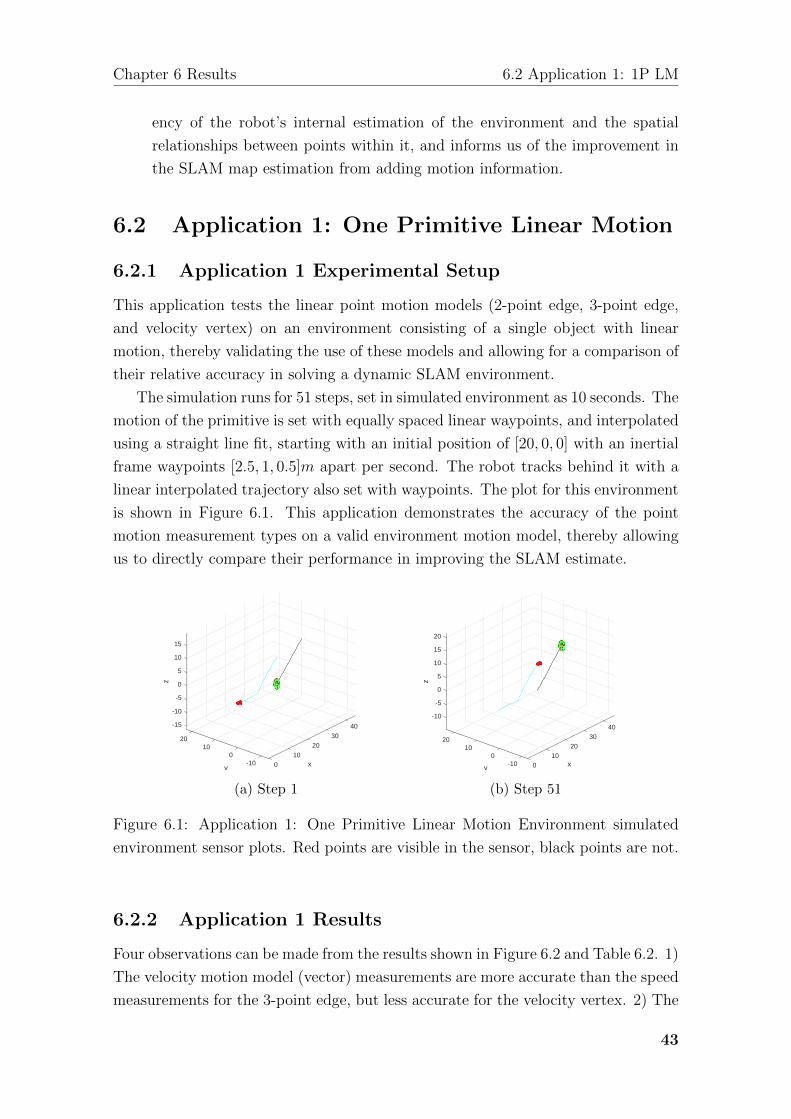
Chapter 6 Results 6.2 Application 1: 1P LM
ency of the robot’s internal estimation of the environment and the spatial
relationships between points within it, and informs us of the improvement in
the SLAM map estimation from adding motion information.
6.2 Application 1: One Primitive Linear Motion
6.2.1 Application 1 Experimental Setup
This application tests the linear point motion models (2-point edge, 3-point edge,
and velocity vertex) on an environment consisting of a single object with linear
motion, thereby validating the use of these models and allowing for a comparison of
their relative accuracy in solving a dynamic SLAM environment.
The simulation runs for 51 steps, set in simulated environment as 10 seconds. The
motion of the primitive is set with equally spaced linear waypoints, and interpolated
using a straight line fit, starting with an initial position of [20, 0, 0] with an inertial
frame waypoints [2.5, 1, 0.5]m apart per second. The robot tracks behind it with a
linear interpolated trajectory also set with waypoints. The plot for this environment
is shown in Figure 6.1. This application demonstrates the accuracy of the point
motion measurement types on a valid environment motion model, thereby allowing
us to directly compare their performance in improving the SLAM estimate.
40-15
30
-10
20
-5
x
0z
5
2010
10
y
15
0 10-10 0
(a) Step 1
40
-10
30
-5
20
0
x
5
z
20
10
10
y
15
20
0 10-10 0
(b) Step 51
Figure 6.1: Application 1: One Primitive Linear Motion Environment simulated
environment sensor plots. Red points are visible in the sensor, black points are not.
6.2.2 Application 1 Results
Four observations can be made from the results shown in Figure 6.2 and Table 6.2. 1)
The velocity motion model (vector) measurements are more accurate than the speed
measurements for the 3-point edge, but less accurate for the velocity vertex. 2) The
43

Chapter 6 Results 6.2 Application 1: 1P LM
40
30
x
20
0
5
15
z
10
1010
y
50
(a) No Motion Estimation
40
30
x
200
2
10
4
10
z
6
y
50
(b) 2-point Edge
4540
3530
25
x
2015
-2
0
10
2
10
4
z
6
y
5 50
(c) 3-point Edge (speed)
40
30
x
200
2
4
10
z
6
10
8
y
50
(d) 3-point Edge (velocity)
40
30
x
200
2
4
10
z
10
6
y
50
(e) Velocity Vertex (speed)
40
30
x
200
2
10
4
10
6
z
8
y
50
(f) Velocity Vertex (velocity)
Figure 6.2: Application 1: One Primitive Linear Motion Results. Red is SLAM
solver final estimate and blue is ground truth. Circles with axes in them are robot
poses and dots are point positions.
most accurate solution is done by the 2-point edge, however it is also an unrealistic
model as in a real world sensor such measurements are difficult to collect. 3) The
velocity vertex is more accurate than the 3-point edge for pure linear motion. 4)
Implementing the linear motion model measurements increases the point position
estimate accuracy at the expense of increased error in the robot trajectory.
44
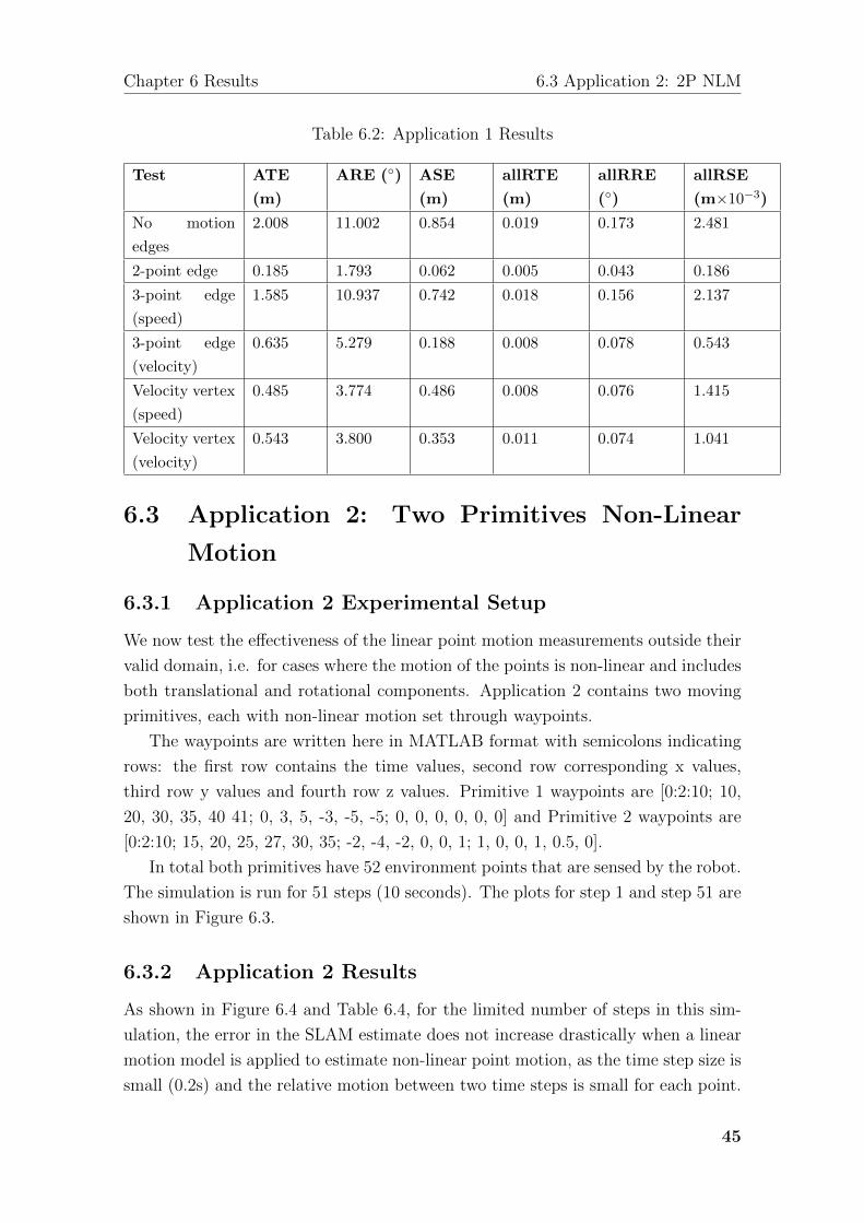
Chapter 6 Results 6.3 Application 2: 2P NLM
Table 6.2: Application 1 Results
Test ATE
(m)
ARE (◦) ASE
(m)
allRTE
(m)
allRRE
(◦)
allRSE
(m×10−3)
No motion
edges
2.008 11.002 0.854 0.019 0.173 2.481
2-point edge 0.185 1.793 0.062 0.005 0.043 0.186
3-point edge
(speed)
1.585 10.937 0.742 0.018 0.156 2.137
3-point edge
(velocity)
0.635 5.279 0.188 0.008 0.078 0.543
Velocity vertex
(speed)
0.485 3.774 0.486 0.008 0.076 1.415
Velocity vertex
(velocity)
0.543 3.800 0.353 0.011 0.074 1.041
6.3 Application 2: Two Primitives Non-Linear
Motion
6.3.1 Application 2 Experimental Setup
We now test the effectiveness of the linear point motion measurements outside their
valid domain, i.e. for cases where the motion of the points is non-linear and includes
both translational and rotational components. Application 2 contains two moving
primitives, each with non-linear motion set through waypoints.
The waypoints are written here in MATLAB format with semicolons indicating
rows: the first row contains the time values, second row corresponding x values,
third row y values and fourth row z values. Primitive 1 waypoints are [0:2:10; 10,
20, 30, 35, 40 41; 0, 3, 5, -3, -5, -5; 0, 0, 0, 0, 0, 0] and Primitive 2 waypoints are
[0:2:10; 15, 20, 25, 27, 30, 35; -2, -4, -2, 0, 0, 1; 1, 0, 0, 1, 0.5, 0].
In total both primitives have 52 environment points that are sensed by the robot.
The simulation is run for 51 steps (10 seconds). The plots for step 1 and step 51 are
shown in Figure 6.3.
6.3.2 Application 2 Results
As shown in Figure 6.4 and Table 6.4, for the limited number of steps in this sim-
ulation, the error in the SLAM estimate does not increase drastically when a linear
motion model is applied to estimate non-linear point motion, as the time step size is
small (0.2s) and the relative motion between two time steps is small for each point.
45

Chapter 6 Results 6.3 Application 2: 2P NLM
50
40-5
30
x
10
0
20
5
z
y
10
0 10
0-10
(a) Step 1
50
40-5
30
x
10
0
20
5
z
y
10
0 10
0-10
(b) Step 51
Figure 6.3: Application 2: Two Primitives Non-Linear Motion Environment simu-
lated environment sensor plots. Red points are visible in the sensor, black points
are not.
Table 6.3: Application 2 Results
Test ATE
(m)
ARE (◦) ASE
(m)
allRTE
(m)
allRRE
(◦)
allRSE
(m×10−3)
No motion
edges
2.039 11.111 0.949 0.021 0.175 1.985
2-point edge 0.278 1.907 0.203 0.006 0.042 0.429
3-point edge
(speed)
0.535 4.964 0.848 0.017 0.123 1.805
3-point edge
(velocity)
1.090 5.836 0.390 0.010 0.089 0.837
Velocity vertex
(speed)
0.657 8.170 0.455 0.010 0.093 0.996
Velocity vertex
(velocity)
0.668 4.215 0.334 0.011 0.073 0.701
In this application, the speed motion models perform better than the velocity mod-
els for both the robot trajectory and map estimate. One reason for this could be
the relative flexibility in the constraint implemented that makes no assumption on
the direction of motion for the point.
46

Chapter 6 Results 6.4 Application 3: 1 Primitive NLM + SP
4035
30-20
25
x
24
z
20515
y
0 105-5
(a) No Motion Estimation
4035
3025-2
x
0
20
2
4
z
2 150
y
10-2-4 5-6
(b) 2-point Edge
4035
3025
x
-2
20
0
4
2
z
1520
y
10-2-4 5-6
(c) 3-point Edge (speed)
4035
3025-2
x
0
20
2
5
z4
15
y
0 105-5
(d) 3-point Edge (velocity)
4035
3025
x
-4
20
-2
4
0
z
152
2
0
y
10-2-4 5-6
(e) Velocity Vertex (speed)
4035
3025-2
x
0
205
2
z
4
150
y
10-5 5
(f) Velocity Vertex (velocity)
Figure 6.4: Application 2: Two Primitives Non-Linear Motion Results. Red is
SLAM solver final estimate and blue is ground truth. Circles with axes in them are
robot poses and dots are point positions.
6.4 Application 3: One Primitive Non-Linear Mo-
tion + Static Points
6.4.1 Application 3 Experimental Setup
We expand the case in section 6.3 to include static points in the scene, that are
repeatedly observed from multiple robot posts in conjuntion with the dynamic points
47

Chapter 6 Results 6.4 Application 3: 1 Primitive NLM + SP
and their motion on the primitive. SLAM research literature shows that loop-closure
improves the SLAM estimation[13]. There are 126 points in this simulation, 100
static and 26 dynamic. Static points are initialised along planes modelling walls,
behind the primitive so that occlusion occurs. Primitive waypoints are set as (using
MATLAB notation as explained in subsection 6.3.1): [0:2:10; 10, 20, 25, 20, 10, 5; 0,
0, 10, 15, 15, 15; 0, 2, 1, 3, ,5 2]. The simulation is run for 51 time steps (simulation
time 10s). The plot of the environment at step 1 and 51 is in Figure 6.5.
30
20-5
0
20
x
5
10
z
10
10
y
15
20
00
(a) Step 1
30
20-5
0
20
x
5
10
z
10
10
y
15
20
00
(b) Step 51
Figure 6.5: Application 1: Two Primitives Non-Linear Motion Environment simu-
lated environment sensor plots. Red points are visible in the sensor, black points
are not.
6.4.2 Application 3 Results
The results in Table 6.4 and Figure 6.6 illustrate that loop-closure from repeated
observation of static points increases the overall SLAM estimation accuracy. How-
ever, applying a linear motion model to non-linear motion can worsen the accuracy
of the SLAM estimate compared to if the system is optimised using repeat meas-
urements of static points alone, particularly for the 3-point edge and velocity vertex
scalar measurements. The 3-point edge (velocity) is the only measure that improves
SLAM estimate for both robot trajectory and point positions, however the exact
reason is difficult to determine.
48

Chapter 6 Results 6.4 Application 3: 1 Primitive NLM + SP
30
20
0
20
5
x
10
z
15
y
1010
0
(a) No Motion Estimation
30
20
0
20
5
x
10
z
15
y
1010
0
(b) 2-point Edge
30
20
0
5
20
x
10z
10
15
y
10
20
00
(c) 3-point Edge (speed)
30
20
0
20
5
x
10z
15
y
1010
0
(d) 3-point Edge (velocity)
30
20
0
20
5
x
10
z
y
15
1010
0
(e) Velocity Vertex (speed)
30
20
0
20
5
x
10
z
15
y
1010
0
(f) Velocity Vertex (velocity)
Figure 6.6: Application 3: One Primitive Non-Linear Motion + Static Points Res-
ults. Red is SLAM solver final estimate and blue is ground truth. Circles with axes
in them are robot poses and dots are point positions. Note subfigure (c) where the
SLAM estimate is noticeably made worse.
49

Chapter 6 Results 6.5 Applications 4 and 5: Constant Motion Primitives
Table 6.4: Application 3 Results
Test ATE
(m)
ARE (◦) ASE
(m)
allRTE
(m)
allRRE
(◦)
allRSE
(m×10−3)
No motion
edges
0.046 0.240 0.061 0.001 0.005 0.164
2-point edge 0.049 0.427 0.036 0.001 0.005 0.098
3-point edge
(speed)
3.813 14.428 0.079 0.029 0.144 0.216
3-point edge
(velocity)
0.026 0.177 0.061 0.001 0.005 0.164
Velocity vertex
(speed)
0.657 8.170 0.455 0.010 0.093 0.996
Velocity vertex
(velocity)
0.275 1.130 0.057 0.002 0.015 0.155
6.5 Applications 4 and 5: Constant Motion Prim-
itives
Applications 4 and 5 test the constant motion vertex, which is the most general
motion model and can estimate the point translation and rotation for the points
associated to an object, provided it is constant for the entire simulation. The en-
vironments in these applications model primitives with constant motion trajectories
and test the accuracy of the SLAM estimate with incorporation of the constant
motion. This is an estimation, where the motion vertex is initialised from the point
measurements by finding the inertial frame relative transform (4.32).
6.5.1 Application 4: Two Primitives Constant Motion Ex-
perimental Setup
In Application 4, the robot follows a figure of 8 trajectory in between 2 objects that
follow a circular trajectory, and observes points on the objects at various times.
The simulation is run for 120 seconds with 121 time steps. In Figure 6.7, primitive
1 (left) has a se(3) constant motion of u1 = [1.2226, 1.4476, 0, 0, 0, 0.105], and
primitive 2 (right) has a constant motion of u2 = [-1.2226, 1.4476, 0, 0, 0, -0.105].
The total number of points from both ellipsoids is 22.
50

Chapter 6 Results 6.5 Applications 4 and 5: Constant Motion Primitives
30-10
30 20
0
z (m
)
1020
x (m)
10
0
y (m)
10 -10
-200-30
(a) Step 1
30-10
30 20
0
z (m
)
1020
x (m)
10
0
y (m)
10 -10
-200-30
(b) Step 121
Figure 6.7: Application 4: Two Primitives Constant Motion Environment simulated
environment sensor plots. Red points are visible in the sensor, black points are not.
6.5.2 Application 5: One Primitive Constant Motion + Static
Points Experimental Setup
In Application 5, the environment consists of an object moving in a screw trajectory
in front of static points created along rectangles. The primitive has a se(3) motion
transform of u = [0.9938, -0.4028, -0.0013, 0.001, 0.0002, 0.06]. There are static
points and dynamic points in the environment. This simulation is also from t=0s
to t=120s with 121 time steps. Robot motion is set via waypoints tracking behind
the primitive. The plot for the environment is shown in Figure 6.8.
Application 5 is tested with and without loop closure. With loop closure, static
points in the environment are observed in the first and final time steps and associated
together. Without loop closure, the static points are not associated and new vertices
are created when the same point is observed again after losing track in the robot
sensor.
6.5.3 Application 4 and 5 Results
From Figures Figure 6.9 and Figure 6.10, and Table 6.5 it can be seen that im-
plementing the constant motion estimation of points in an environment, where the
motion model is valid, improves the general accuracy of the environment map. How-
ever, often there is a tradeoff between improving the map estimate and a less accurate
robot trajectory estimate.
51

Chapter 6 Results 6.5 Applications 4 and 5: Constant Motion Primitives
-103040
0
z (m
)
10
30 20
20
x (m)y (m)
20 1010
00
(a) Step 1
-103040
0
z (m
)
10
30 20
20
x (m)y (m)
20 1010
00
(b) Step 121
Figure 6.8: Application 5: One Primitive Constant Motion + Static Points simulated
environment sensor plots. Red points are visible in the sensor, black points are not.
-5
30 20
0
5
10
z (m
)
20
10
x (m)y (m)
0
15
10 -10
-200
Figure 6.9: Application 4 solver results. Large dots represent robot positions and
small dots point locations. Green colour denotes ground truth, blue denotes SLAM
solution with the SE(3) transform and red denotes the SLAM solution without the
SE(3) transform.
52

Chapter 6 Results 6.5 Applications 4 and 5: Constant Motion Primitives
30-540
0
5
20
z (m
) 10
30
15
x (m)y (m)
10
20
20
010
0
(a) Without Loop Closure
30-5
0
40
5
20
z (m
) 10
30
15
20
x (m)y (m)
1020
010
0
(b) With Loop Closure
Figure 6.10: Application 5 solver results. Large dots represent robot positions and
small dots point locations. Green colour denotes ground truth, blue denotes SLAM
solution with the SE(3) transform and red denotes the SLAM solution without the
SE(3) transform.
Table 6.5: Application 4 and 5 Results ‘a’ and ‘b’ indicate the application results
with and without without application of the constant motion vertex respectively.
‘wolc’ means without loop closure, ‘wlc’ means with loop closure.
Application
Setup
ATE
(m)
ARE (◦) ASE
(m)
allRTE
(m)
allRRE
(◦)
allRSE
(m×10−3)
4-a 5.442 15.625 1.968 0.019 0.099 4.076
4-b 2.282 7.566 0.650 0.009 0.035 1.442
5-wolc-a 0.592 5.228 1.234 0.008 0.056 1.091
5-wolc-b 0.428 1.651 0.126 0.002 0.010 0.113
5-wlc-a 0.100 0.937 0.163 0.002 0.013 0.170
5-wlc-b 0.195 1.232 0.074 0.001 0.007 0.072
53

Chapter 7
Conclusion
The goal of this honours thesis is to conceptualise and develop the front-end of
the DO-SLAM Framework (chapter 5), and use it to test the validity and accuracy
of different motion measurement and estimations models that are integrated in a
SLAM algorithm. I evaluate the performance of six theoretical motion measurement
and estimation models (section 4.5), which are tested on simulated data.
I also describe the Dynamic Object SLAM (DO-SLAM) framework which is the
broader subject of the research program I am a part of. DO-SLAM incorporates
methods of adding the structure [5] and motion [2] of objects in the environment in
order to improve the SLAM estimation. My contributions to this research program
include helping conceptualise the overall structure of the framework (section 4.1),
adding the functionality to create primitives with abstract surface representations
(subsection 5.1.4), designing and implementing occlusion (section 4.4) in the abstract
simulated environment sensors, adding functionality to create graph files with point
motion measurements and constraints, and testing of the algorithms on simulated
data (chapter 6).
From the results in chapter 6, we can see that in general adding more informa-
tion to the SLAM system for dynamic environments improves the SLAM estimate
accuracy, in particular for environments with only dynamic objects. However, the
improvement to the map and robot trajectory estimate is decreased in cases where
the solution motion model is not valid for the actual motion of the corresponding
points in the environment. The measurements created according to linear point
motion models are not robust in cases where they the object motion is actually
non-linear, and in some cases reduces the accuracy of the SLAM estimate, particu-
larly when used in conjunction with the conventional static point tracking and loop
closure methods (see sections section 6.2 and section 6.4).
The constant motion vertex is an improvement on the linear point motion as-
sumptions as it uses the SE(3) transformation of the object in the inertial frame,
and is the most generalised which results in consistent improvement in the SLAM
estimation when applied to points and objects where it is a valid model, as evid-
enced in subsection 6.5.3. Furthermore, through deriving geometric relationships we
54

Chapter 7 Conclusion
show that the constant motion transform in the inertial frame for a set of grouped
points moving in a 3D environment can be derived without explicitly requiring their
geometric relationship with their associated object (subsection 4.5.4), which ex-
pands the application potential of this method. As it is an estimation that provides
a structure to the already existing point measurements from the robot sensor, it
is applicable to a real-world environment in comparison to the linear point motion
models which all assume that there independent measurements of the point’s motion
or average velocity can be obtained.
To further develop this concept, the constant motion assumption needs to be fur-
ther developed as a derivation or in implementation to make it robust and applicable
in a real world environment. Segmenting the motion of a group of points by time
step and applying the constant motion assumption for a set of time steps instead of
the entire observation time is one possible method of doing this. Furthermore, we
assume that the data association problem is solved in the simulated environment,
however in the real world data association is a significant task and additional tech-
niques such as CNN based image recognition will need to be integrated on camera
sensor data to data associate and track objects. The current developed algorithms
also require a rigid body assumption to be a valid model the object, which needs to
be adapted further to operate with real world deformable bodies such as pedestrians
that commonly form part of a dynamic environment.
55

Appendix A
Appendix 1
A.1 Unit Tests
The correct implementation of the point motion model in the solver algorithm is
demonstrated by unit tests, where we manually construct a simple system of 3
points moving over 3 time steps with a robot observing it, without using the front-
end of the framework. The motion of the points is set to be linear for the 2-point
edge, 3-point edge and velocity vertex motion measurements to test cases where the
algorithm’s motion model is valid.
The points are initialised as part of an object in the object frame. The constant
motion is applied to the object, and the point positions are found in the inertial frame
to construct the sensor measurement edges and motion measurement edges/vertices.
Error settings are in Table A.1 and results for all of the unit tests are in Table A.2,
where the error measures have been explained in section section 6.1. Figures A.2
and A.1 show the visual plot of the results.
Table A.1: Unit test config noise settings
Label Measure Set as Value
stdPosePrior Prior for the sensor pose
error
0.005m translation, 1
degree error in each
Axis-Angle dimension.
[0.0050, 0.0050,
0.0050, 0.0175,
0.0175, 0.0175]
stdPosePose Odometry/IMU pose
change error
0.04m translation and
2 degree in each Axis-
Angle dimension.
[0.0400, 0.0400,
0.0400, 0.0873,
0.0873, 0.0873]
stdPointPrior Prior for initialising a
point based on measure-
ments
0.01m position error in
R3 (inertial frame)
[0.01, 0.01, 0.01]
stdPosePoint Point measurement er-
ror in sensor frame co-
ordinates
0.04m position error in
R3 (sensor frame)
[0.04, 0.04 0.04]
56

Appendix A Appendix 1 A.1 Unit Tests
Table A.2: Unit test Results
Test ATE
(m)
ARE (◦) ASE
(m)
allRTE
(m)
allRRE
(◦)
allRSE
(m×10−3)
No motion
edges
0.206 2.507 0.778 0.116 1.254 147.086
2-point edge 0.245 3.015 0.260 0.132 1.489 46.009
3-point edge
(scalar)
0.169 2.932 0.741 0.086 1.443 139.250
3-point edge
(vector)
0.169 2.924 0.411 0.081 1.455 78.293
Velocity vertex
(scalar)
0.154 2.918 0.796 0.081 1.454 147.391
Velocity vertex
(vector)
0.177 2.838 0.411 0.085 1.409 77.127
Constant Mo-
tion Vertex
0.233 2.174 0.634 0.113 1.087 114.749
0
4
2
62
4
4
z
xy
0 2
6
-2 0
Figure A.1: Unit Test Results for the constant motion vertex explained in subsec-
tion 4.5.4. The motion input includes both translation and rotation. Red is final
solution estimate and blue is ground truth. Circles with axes are robot poses and
dots are point positions.
57
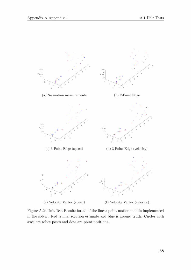
Appendix A Appendix 1 A.1 Unit Tests
8
7
6
5
x
4
3
0
0.5z
2
1
2
1.5
y
1 10
0-1
(a) No motion measurements
8
7
6
5
x
4
30
0.5
2 2
z
1
y
1
1.5
10
0-1
(b) 2-Point Edge
8
7
6
5
x
4
30
0.5
2
1
z
1
y
1.5
10-1 0
(c) 3-Point Edge (speed)
8
7
6
5
x
4
3
2
0
0.5z
1
1
y
10
0-1
(d) 3-Point Edge (velocity)
8
7
6
5
x
4
3
0
2
1z
1
y
2
0 1-1
0
(e) Velocity Vertex (speed)
8
7
6
5
x
4
3
0
2 2
0.5
z
1
y
11
00-1
(f) Velocity Vertex (velocity)
Figure A.2: Unit Test Results for all of the linear point motion models implemented
in the solver. Red is final solution estimate and blue is ground truth. Circles with
axes are robot poses and dots are point positions.
58

Bibliography
[1] “MathWorks transform cartesian coordinates to spherical - cart2sph,” https:
//au.mathworks.com/help/matlab/ref/cart2sph.html, accessed: 2017-10-21.
[2] M. Henein, Y. Vyas, J. Trumpf, V. Ila, and R. Mahony, “Simultaneous local-
ization, mapping and tracking in dynamic environments,” in 2018 IEEE Inter-
national Conference on Robotics and Automation. Institute of Electrical and
Electronics Engineers (IEEE), 2018, submission.
[3] H. Durrant-Whyte and T. Bailey, “Simultaneous localization and mapping:
part i,” IEEE Robotics Automation Magazine, vol. 13, no. 2, pp. 99–110, June
2006.
[4] F. Dellaert and M. Kaess, “Square root SAM: Simultaneous localization and
mapping via square root information smoothing,” The International Journal of
Robotics Research, vol. 25, no. 12, pp. 1181–1203, dec 2006.
[5] M. Henein, M. Abello, V. Ila, and R. Mahony, “Exploring the effect of meta-
structural information on the global consistency of slam,” in 2017 IEEE/RSJ
International Conference on Intelligent Robots and Systems, 2017.
[6] A. Cunningham, V. Indelman, and F. Dellaert, “DDF-SAM 2.0: Consistent
distributed smoothing and mapping,” in 2013 IEEE International Conference
on Robotics and Automation. Institute of Electrical and Electronics Engineers
(IEEE), may 2013.
[7] A. Cunningham, K. M. Wurm, W. Burgard, and F. Dellaert, “Fully distributed
scalable smoothing and mapping with robust multi-robot data association,” in
2012 IEEE International Conference on Robotics and Automation. Institute
of Electrical and Electronics Engineers (IEEE), may 2012.
[8] R. F. Salas-Moreno, R. A. Newcombe, H. Strasdat, P. H. Kelly, and A. J.
Davison, “SLAM++: Simultaneous localisation and mapping at the level of
objects,” in 2013 IEEE Conference on Computer Vision and Pattern Recogni-
tion. Institute of Electrical and Electronics Engineers (IEEE), jun 2013.
[9] A. Walcott-Bryant, M. Kaess, H. Johannsson, and J. J. Leonard, “Dynamic
pose graph SLAM: Long-term mapping in low dynamic environments,” in 2012
59

Appendix A Appendix 1 A.1 Unit Tests
IEEE/RSJ International Conference on Intelligent Robots and Systems. In-
stitute of Electrical and Electronics Engineers (IEEE), oct 2012.
[10] C. Bibby and I. Reid, “Simultaneous localisation and mapping in dynamic envir-
onments (slamide) with reversible data association,” in Proceedings of Robotics
Science and Systems, vol. 117, 2007, p. 118.
[11] C.-C. Wang, C. Thorpe, S. Thrun, M. Hebert, and H. Durrant-Whyte,
“Simultaneous localization, mapping and moving object tracking,” The
International Journal of Robotics Research, vol. 26, no. 9, pp. 889–916, 2007.
[Online]. Available: https://doi.org/10.1177/0278364907081229
[12] J.-L. Blanco, “A tutorial on se(3) transformation parameterizations and on-
manifold optimization,” Universidad de Malaga, Tech. Rep., 2014.
[13] J. Engel, V. Koltun, and D. Cremers, “Direct sparse odometry,” ArXiv e-prints,
Jul. 2016.
60